ADA1: Chapter8, Correlation & Regressionjames/chapter8f.pdf · Chapter 8: Correlation & Regression ADA1 November 12, 2017 13 / 105. Chapter 8: Correlation & Regression ADA1 November

Chapter 8: Correlation & Regression

We can think of ANOVA and the two-sample t-test as applicable tosituations where there is a response variable which is quantitative, andanother variable that indicates group membership, which we might thinkof a as categorical predictor variable.

In the slides on categorical data, all varaibles are categorical, and we keeptrack of the counts of observation in each category or combination ofcategories.

In this section, we analyze cases where we have multiple quantitativevariables.

ADA1 November 12, 2017 1 / 105


In the simplest case, there are two quantitative variables. Examplesinclude the following:

I heights of fathers and sons (this is a famous example from Galton,Darwin’s cousin)

I ages of husbands and wifes

I systolic versus diastolic pressure for a set of patients

I high school GPA and college GPA

I college GPA and GRE scores

I MCAT scores before and after a training course

In the past, we might have analyzed pre versus post data using atwo-sample t-test to see whether there was a difference. It is also possibleto try to quantify the relationship—instead of just asking whether the twosets of scores are different, or getting an interval for the average difference,we can also try to predict the new score based on the old score, and theamount of improvmenet might depend on the old score.

ADA1 November 12, 2017 2 / 105


Here is some example data for husbands and wives. Heights are in mm.

Couple HusbandAge HusbandHeight WifeAge WifeHeight

1 49 1809 43 1590

2 25 1841 28 1560

3 40 1659 30 1620

4 52 1779 57 1540

5 58 1616 52 1420

6 32 1695 27 1660

7 43 1730 52 1610

8 47 1740 43 1580

9 31 1685 23 1610

10 26 1735 25 1590

11 40 1713 39 1610

12 35 1736 32 1700

ADA1 November 12, 2017 3 / 105

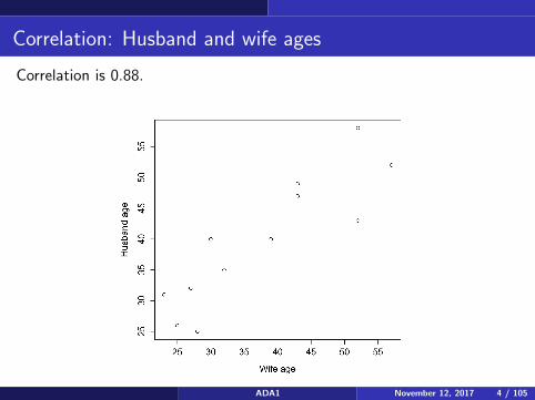
Correlation: Husband and wife ages

Correlation is 0.88.

ADA1 November 12, 2017 4 / 105

Correlation: Husband and wife heights

Correlation is 0.18 with outlier, but -0.54 without outlier.

ADA1 November 12, 2017 5 / 105

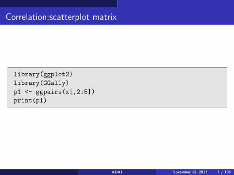
Correlation: scatterplot matrix

pairs(x[,2:5]) allows you to look at all data simultaneously.

ADA1 November 12, 2017 6 / 105

Correlation:scatterplot matrix

library(ggplot2)

library(GGally)

p1 <- ggpairs(x[,2:5])

print(p1)

ADA1 November 12, 2017 7 / 105

Correlation: scatterplot matrix

ADA1 November 12, 2017 8 / 105


For a data set like this, you might not expect age to be significantlycorrelated with height for either men or women (but you could check).You could also check whether differences in couples ages are correlatedwith differences in their heights. The correlation between two variables isdone as follows:

cor(x$WifeAge,x$HusbandAge)

Note that the correlation is looking at something different than the t test.A t-test for this data might look at whether the husbands and wives hadthe same average age. The correlation looks at whether younger wivestend to have younger husbands and older husbands tend to have olderwives, whether or not there a difference in the ages overall. Similarly forheight. Even if husbands tend to be taller than wives, that doesn’tnecessarily mean that there is a relationship between the heights forcouples.

ADA1 November 12, 2017 9 / 105

Pairwise Correlations

The pairwise correlations for an entire dataset can be done as follows.What would it mean to report the correlation between the Couple variableand the other variables? Here I only get the correlations for variables otherthan the ID variable.

options(digits=4) # done so that the output fits

#on the screen!

cor(x[,2:5])

HusbandAge HusbandHeight WifeAge WifeHeight

HusbandAge 1.0000 -0.24716 0.88003 -0.5741

HusbandHeight -0.2472 1.00000 0.02124 0.1783

WifeAge 0.8800 0.02124 1.00000 -0.5370

WifeHeight -0.5741 0.17834 -0.53699 1.0000

ADA1 November 12, 2017 10 / 105


The correlation measures the linear relationship between variables X andY as seen in a scatterplot. The sample correlation between X1, . . . ,Xn andY1, . . . ,Yn is denoted by r has the following properties

I −1 ≤ r ≤ 1I if Yi tends to increase linearly with Xi , then r > 0I if Yi tends to decrease linearly with Xi , then r < 0I if there is a perfect linear relationship between X and Y , then r = 1

(points fall on a line with positive slope)I if there is a perfect negative relationship between X and Y , then

r = −1 (points fall on a line with negative slope)I the closer the points (Xi ,Yi ) are to a straight line, the closer r is to 1

or −1I r is not affected by linear transformations (i.e., converting from inches

to centimeters, Fahrenheit to Celsius, etc.I the correlation is symmetric: the correlation between X and Y is the

same as the correlation between Y and XADA1 November 12, 2017 11 / 105


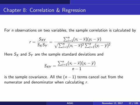
For n observations on two variables, the sample correlation is calculated by

r =SXYSXSY

=

∑ni=1(xi − x)(yi − y)√∑n

i=1(xi − x)2∑n

i=1(yi − y)2

Here SX and SY are the sample standard deviations and

SXY =

∑ni=1(xi − x)(yi − y)

n − 1

is the sample covariance. All the (n − 1) terms cancel out from thenumerator and denominator when calculating r .

ADA1 November 12, 2017 12 / 105


ADA1 November 12, 2017 13 / 105


ADA1 November 12, 2017 14 / 105


CIs and hypothesis tests can be done for correlations using cor.test().The test is usually based on testing whether the population correlation ρ isequal to 0, so

H0 : ρ = 0

and you can have either a two-sided or one-sided alternative hypothesis.We think of r as a sample estimate of ρ, the Greek letter for r . The test isbased on a t-statistic which has the formula

tobs = r

√n − 2

1− r2

and this is compared to a t distribution with n − 2 degrees of freedom. Asusual, you can rely on R to do the test and get the CI.

ADA1 November 12, 2017 15 / 105

Correlation

The t distribution derivation of the p-value and CI assume that the jointdistribution of X and Y follow what is called a bivariate normaldistribution. A sufficient condition for this is that X and Y eachindividually have normal distributions, so you can do usual tests ordiagnostics for normality. Similar to the t-test, the correlation is sensitiveto outliers. For the husband and wife data, the sample sizes are small,making it difficult to detect outliers. However, there is not clear evidenceof non-normality.

ADA1 November 12, 2017 16 / 105


ADA1 November 12, 2017 17 / 105


Shairpo-Wilk’s tests for normality would all be not rejected, although thesample sizes are quite small for detecting deviations from normality:

> shapiro.test(x$HusbandAge)$p.value

[1] 0.8934

> shapiro.test(x$WifeAge)$p.value

[1] 0.2461

> shapiro.test(x$WifeHeight)$p.value

[1] 0.1304

> shapiro.test(x$HusbandHeight)$p.value

[1] 0.986

ADA1 November 12, 2017 18 / 105

Correlation

Here we test whether ages are significantly correlated and also whetherheights are positively correlated.

> cor.test(x$WifeAge,x$HusbandAge)

Pearson’s product-moment correlation

data: x$WifeAge and x$HusbandAge

t = 5.9, df = 10, p-value = 2e-04

alternative hypothesis: true correlation is not equal to 0

95 percent confidence interval:

0.6185 0.9660

ADA1 November 12, 2017 19 / 105

Correlation

Here we test whether ages are significantly correlated and also whetherheights are positively correlated.

> cor.test(x$WifeHeight,x$HusbandHeight)


data: x$WifeHeight and x$HusbandHeight

t = 0.57, df = 10, p-value = 0.6



-0.4407 0.6824

sample estimates:

cor

0.1783

ADA1 November 12, 2017 20 / 105

Correlation

We might also test the heights with the bivariate outlier removed:

> cor.test(x$WifeHeight[x$WifeHeight>1450],x$HusbandHeight[x$WifeHeight>1450])


data: x$WifeHeight[x$WifeHeight > 1450] and x$HusbandHeight[x$WifeHeight > 1450]

t = -1.9, df = 9, p-value = 0.1



-0.8559 0.1078

sample estimates:

cor

-0.5261

ADA1 November 12, 2017 21 / 105

Correlation

Removing the outlier changes the direction of the correlation (frompositive to negative). The result is still not significant at the α = 0.05level, although the p-value is 0.1, suggesting slight evidence against thenull hypothesis of no relationship between heights of husbands and wives.Note that the negative correlation here means that, with the one outliercouple removed, taller wives tended to be associated with shorterhusbands and vice versa.

ADA1 November 12, 2017 22 / 105

Correlation

A nonparametric approach for dealing with outliers or otherwise nonnormaldistributions for the variables being correlated is to rank the data withineach sample and then compute the usual correlation on the ranked data.Note that in the Wilcoxon two-sample test, you pool the data first andthen rank the data. For the Spearman correlation, you rank each groupseparately.

The idea is that large observations will have large ranks in both groups, sothat if the data is correlated, large ranks will tend to get paired with largeranks, and small ranks will tend to get paired with small ranks if the datais correlated. If the data are uncorrelated, then the ranks will be randomwith respect to each other.

ADA1 November 12, 2017 23 / 105

The Spearman correlation is implemented in cor.test() using the optionmethod=’’spearman’’. Note that the correlation is negative using theSpearman ranking even with the outlier, but the correlation was positive using theusual (Pearson) correlation. The Pearson correlation was negative when theoutlier was removed. Since the results depended so much on the presence of asingle observation, I would be more comfortable with the Spearman correlation forthis example.

cor.test(x$WifeHeight,x$HusbandHeight,method="spearman")

Spearman’s rank correlation rho

data: x$WifeHeight and x$HusbandHeight

S = 370, p-value = 0.3

alternative hypothesis: true rho is not equal to 0

sample estimates:

rho

-0.3034

ADA1 November 12, 2017 24 / 105


A more extreme example of an outlier. Here the correlation changes from0 to negative.

ADA1 November 12, 2017 25 / 105

Correlation

Something to be careful of is that if you have many variables (which oftenoccurs), then testing every pair of variables for a significant correlationleads to multiple comparison problems, for which you might want to use aBonferroni correction, or limit yourself to only testing a small number ofpairs of variable that are interesting a priori.

ADA1 November 12, 2017 26 / 105

Regression

In regression, we try to make a model that predicts the average responseof one quantitative variable given one or more predictor variables. We startwith the case that there is one predictor variable, X , and one response, Y ,which is called simple linear regression.

Unlike correlation, the model depends on which variable is the predictorand which is the response. While the correlation of x and y is the same asthe correlation of y and x , the regression of y on x will generally lead to adifferent model than regressing on x on y . In the phrase “regressing y onx”, we mean that y is the response and x is the predictor.

ADA1 November 12, 2017 27 / 105

Regression

In the basic regression model, we assume that the average value of Y hasa linear relationship to X , and we write

y = β0 + β1x

Here β0 is the coefficient and β1 is the slope of the line. This is similar toequations of lines from courses like College Algebra where you write

y = a + bx

ory = mx + b

But we think of β0 and β1 as unknown parameters, similar to µ for themean of a normal distribution. One possible goal of a regression analysis isto make good estimates of β0 and β1.

ADA1 November 12, 2017 28 / 105

Regression

Review of lines, slopes, and intercepts. The slope is the number of unitsthat y changes for a change of 1 unit in x . The intercept (or y -intercept)is where the line intersects the y -axis.

ADA1 November 12, 2017 29 / 105

Regression

In real data, the points almost never fall exactly on a line, but there mightbe a line that describes the overall trend. (This is sometimes even calledthe trend line). Given a set of points, which line through the points is“best”?

ADA1 November 12, 2017 30 / 105

Regression

Husband and wife age example.

ADA1 November 12, 2017 31 / 105

Regression

Husband and wife age example. Here we plot the line y = x . Note that 9 out of

12 points are above the line—for the majority of couples, the husband was older

than the wife. The points seem a little shifted up compared to the line.

ADA1 November 12, 2017 32 / 105

Now we’ve added the usual regression line in black. It has a smaller slope but a

higher intercept. The lines seem to make similar predictions at higher ages, but

the black line seems a better fit to the data for the lower ages. Although this

doesn’t always happen, exactly half of the points are above the black line.

ADA1 November 12, 2017 33 / 105

Regression

It is a little difficult to tell visually which line is best. Here is a third line,which is based on regressing the wives’ heights on the husbands heights.

ADA1 November 12, 2017 34 / 105

Regression

It is difficult to tell which line is “best” or even what is meant by a bestline through the data. What to do?One possible solution to the problem is to consider all possible lines of theform

y = β0 + β1x

or hereHusband height = β0 + β1 × (Wife height)

In other words, consider all possible choices of β0 and β1 and pick the onethat minimizes some criterion. The most common criterion used is theleast squares criterion—here you pick β0 and β1 that minimize

n∑i=1

[yi − (β0 + β1xi )]2

ADA1 November 12, 2017 35 / 105

Regression

Graphically, this means minimizing the sum of squared deviations fromeach point to the line.

ADA1 November 12, 2017 36 / 105

Regression

Rather than testing all possible choices of β0 and β1, formulas are knownfor the optimal choices to minimize the sum of squares. We think of theseoptimal values as estimates of the true, unknown population parametersβ0 and β1. We use b0 or β0 to mean an estimate of β0 and b1 or β1 tomean an estimate of β1:

b1 = β1 =

∑i (xi − x)(yi − y)∑

i (xi − x)2= r

SYSX

b0 = β0 = y − b1x

Here r is the Pearson (unranked) correlation coefficient, and SX and SYare the sample standard deviations. Note that if r is positive if, and onlyif, b1 is positive. Similarly, if one is negative the other is negative. In otherwords, r has the same sign as the slope of the regression line.

ADA1 November 12, 2017 37 / 105

Regression

The equation for the regression line is

y = b0 + b1x

where x is an value (not just values that were observed), and b0 and b1were defined on the previous slide. The notation y is used to mean thepredicted or average value of y for the given x value. You can think of itas meaning the best guess for y if a new observation will have the given xvalue.

A special thing to note about the regression line is that it necessarilypasses through the point (x , y).

ADA1 November 12, 2017 38 / 105

Regression: scatterplot with least squares line

Options make the dots solid and a bit bigger.

plot(WifeAge,HusbandAge,xlim=c(20,60),ylim=c(20,60),xlab=

"Wife Age", ylab="Husband Age", pch=16,

cex=1.5,cex.axis=1.3,cex.lab=1.3)

abline(model1,lwd=3)

ADA1 November 12, 2017 39 / 105

Regression: scatterplot with least squares line

You can always customize your plot by adding to it. For example you canadd the point (x , y). You can also add reference lines, points, annotationsusing text at your own specified coordinates, etc.

points(mean(WifeAge),mean(HusbandAge),pch=17,col=’’red’’)

text(40,30,’’r = 0.88’’,cex=1.5)

text(25,55,’’Hi Mom!’’,cex=2)

lines(c(20,60),c(40,40),lty=2,lwd=2)

The points statement adds a red triangle at the mean of both ages, whichis the point (37.58, 39.83). If a single coordinate is specified by thepoints() function, it adds that point to the plot. To add a curve or lineto a plot, you can use points() with x and y vectors (just like theoriginal data). For lines(), you specify the beginning and ending x and ycoordinates, and R fills in the line.

ADA1 November 12, 2017 40 / 105

Regression

To fit a linear regression model in R, you can use the lm() command,which is similar to aov().The following assumes you have the file couple.txt in the same directoryas your R session:

x <- read.table("couples.txt",header=T)

attach(x)

model1 <- lm(HusbandAge ~ WifeAge)

summary(model1)

ADA1 November 12, 2017 41 / 105

Regression

Call:

lm(formula = HusbandAge ~ WifeAge)

Residuals:

Min 1Q Median 3Q Max

-8.1066 -3.2607 -0.0125 3.4311 6.8934

Coefficients:

Estimate Std. Error t value Pr(>|t|)

(Intercept) 10.4447 5.2350 1.995 0.073980 .

WifeAge 0.7820 0.1334 5.860 0.000159 ***

---

Signif. codes: 0 *** 0.001 ** 0.01 * 0.05 . 0.1 1

Residual standard error: 5.197 on 10 degrees of freedom

Multiple R-squared: 0.7745, Adjusted R-squared: 0.7519

F-statistic: 34.34 on 1 and 10 DF, p-value: 0.0001595

ADA1 November 12, 2017 42 / 105

Regression

The lm() command generates a table similar to the ANOVA tablegenerated by aov().

To go through some elements in the table, it first fives the formula used togenerate the output. This is useful when you have generated severalmodels, say model1, model2, model3, ... and you can’t rememberhow you generated the model. For example, you might have one modelwith an outlier removed, another model with one of the variables on alog-transformed scale, etc.

The next couple lines deal with residuals. Residuals are the differencebetween theobserved and fitted values, That is

yi − yi = yi − (b0 + b1xi )

ADA1 November 12, 2017 43 / 105

Regression

From the web:

www.shodor.org/media/M/T/l/mYzliZjY4ZDc0NjI3YWQ3YWVlM2MzZmUzN2MwOWY.jpg

ADA1 November 12, 2017 44 / 105

Regression

The next part gives a table similar to ANOVA. Here we get the estimatesfor the coefficients, b0 and b1 in the first quantitative column. We also getstandard errors for these, corresponding t-values and p-values. Thep-values are based on testing the null hypotheses

H0 : β0 = 0

andH0 : β1 = 0

The first null hypothesis says that the intercept is 0. For this problem, thisis not very meaningful, as it would mean that the husband of 0-yr oldwoman would also be predicted to be a 0-yr old!

Often the intercept term is not very meaningful in the model. The secondnull hypothesis is that the slope is 0, which would mean that the wife’sage increasing would not be associated with the husband’s age increasing.

ADA1 November 12, 2017 45 / 105

Regression

For this eample, we get a significant result for the wife’s age. This means thatthe wife’s age has some statistically signficant ability to predict the husband’sage. The coefficients give the model

Mean Husband’s Age = 10.4447 + 0.7820× (Wife’s Age)

The low p-value for the Wife’s age, suggest that the coefficient 0.7820 isstatistically significantly different from 0. This means that the data show there isevidence that the wife’s age is associated with the husband’s age. The coefficientof 0.7820 means that for each year of increase in the wife’s age, the meanhusband’s age is predicted to increase by 0.782 years.

As an example, based on this model, a 20-yr old women who was married wouldbe predicted to have a husband who was

10.4447 + (0.782)(30) = 33.9

or about 34 years old. A 50 yr-old women would be predicted to have husbandwho was

10.4447 + (0.782)(55) = 53.5

ADA1 November 12, 2017 46 / 105

Regression

The fitted values are found by plugging in the observed x values (Wifeages) into the regression equation. This gives the expected husband agesfor each wife. They are given automatically using

model1$fitted.values

1 2 3 4 5 6 7 8

44.06894 32.33956 33.90348 55.01637 51.10658 31.55760 51.10658 44.06894

9 10 11 12

28.42976 29.99368 40.94111 35.46740

x$WifeAge

[1] 43 28 30 57 52 27 52 43 23 25 39 32

For example, if the wife is 43, the regression equation predicts10.4447 + (0.782)(43) = 44.069 for the husband age.

ADA1 November 12, 2017 47 / 105

Regression

To see what is stored in model1, type

names(model1)

# [1] "coefficients" "residuals" "effects" "rank"

# [5] "fitted.values" "assign" "qr" "df.residual"

# [9] "xlevels" "call" "terms" "model"

The residuals are also stored, which are the observed husband ages minusthe fitted values.

ei = yi − yi

ADA1 November 12, 2017 48 / 105

Regression: ANOVA table

More details about the regression can be obtained using the anova()

command on the model1 object:

> anova(model1)

Analysis of Variance Table

Response: HusbandAge

Df Sum Sq Mean Sq F value Pr(>F)

WifeAge 1 927.53 927.53 34.336 0.0001595 ***

Residuals 10 270.13 27.01

Here the sum of squared residuals, sum(model1$residuals2) is 270.13.

ADA1 November 12, 2017 49 / 105

Regression: ANOVA table

Other components from the table are (SS means sums of squares):

Residual SS =n∑

i=1

e2i

Total SS =n∑

i=1

(yi − y)2

Regression SS = b1

n∑i=1

(xi − x)(yi − y)

Regression SS = Total SS− Residual SS

R2 =Regression SS

Total SS= r2

The Mean Square values in the table are the SS values divided by the degrees of

freedom. The degrees of freedom is n − 2 for the residuals and 1 for the 1

predictor. The F statistic is MSR/MSE (Measn square for regression divided by

mean square error), and the p-value can be based on the F statistic.

ADA1 November 12, 2017 50 / 105

Regression

Note that R2 = 1 occurs when the Regression SS is equal to the Total SS.This means that the Residual SS is 0, so all of the points fall on the line.In this case, r = 1 and R2 = 1.

On the other hand, R2 = 0 means that the Total SS is equal to theResidual SS, so the Regression SS is 0. We can think of the Regression SSand Residual SS as partitioning the Total SS:

Total SS = Regression SS + Residual SS orRegression SS

Total SS+

Residual SS

Total SS= 1

If a large proportion of the Total SS is from the Regression rather thanfrom Residuals, then R2 is high. It is common to say that R2 is a measureof how much variation is explained by the predictor variable(s). This phraseshould be used cautiously because it doesn’t refer to a causal explanation.

ADA1 November 12, 2017 51 / 105

Regression

For the husband and wife and example for ages, the R2 value was 0.77.This means that 77% of the variation in husband ages was “explained by”variation in the wife ages. Since R2 is just the correlation squared,regressing wife ages on husband ages would also result in R2 = 0.77, and77% of the variation in wife ages would be “explained by” variation inhusband ages. Typically, you want the R2 value to be high, since thismeans you can use one variable (or a set of variables) to predict anothervariable.

ADA1 November 12, 2017 52 / 105

Regression

The least-squares line is mathematically well-defined and can be calculatedwithout thinking about the data probabilitistically. However, p-values andtests of significance assume the data follow a probabilistic model withsome assumptions. Assumptions for regression include the following:

I each pair (xi , yi ) is independent

I The expected value of y is a linear function of x : E (y) = β0 + β1x ,sometimes denoted µY |X

I the variability of y is the same for each fixed value of x . This issometimes denoted σ2y |x

I the distribuiton of y given x is normally distributed with meanβ0 + β1x and variance σ2y |x

I in the model, x is not treated as random

ADA1 November 12, 2017 53 / 105

Regression

Note that the assumption that the variance is the same regardless of x issimilar to the assumption of equal variance in ANOVA.

ADA1 November 12, 2017 54 / 105

Regression

Less formally, the assumptions in their order of importance, are:

1. Validity. Most importantly, the data you are analyzing should map tothe research question you are trying to answer. This sounds obviousbut is often overlooked or ignored because it can be inconvenient.

2. Additivity and Linearity. The most important mathematicalassumption of the regression model is that its deterministiccomponent is a linear function of the separate predictors.

3. Independence of errors (i.e., residuals). This assumption dependson how the data were collected.

4. Equal variance of errors.

5. Normality of errors.

It is easy to focus on the last two (especially when teaching) because thefirst assumptions depend on the scientific context and are not possible toassess just looking at the data in a spreadsheet.

ADA1 November 12, 2017 55 / 105

Regression

To get back to the regression model, the parameters of the model are β0,β1 and σ2 (which we might call σ2Y |X , but it is the same for every x).

Usually σ2 is not directly of interest but is necessary to estimate in orderto do hypothesis tests and confidence intervals for the other parameters.

σ2Y |X is estimated by

s2Y |X = Residual MS =Residual SS

Residual df=

∑i (yi − yi )

2

n − 2

This formula is similar to the sample variance, but we subtract thepredicted values for y instead of the mean for y , y , and we divide by n− 2instead of dividing by n − 1. We can think of this as two degrees offreedom being lost since β0 and β1 need to be estimated. Usually, thesample variance uses n − 1 in the denominator due to one degree offreedom being lost for estimating µY with y .

ADA1 November 12, 2017 56 / 105

Regression

Recall that there are observed residuals, which are observed minus fittedvalues, and unobserved residuals:

ei = yi − yi = yi − (b0 + b1)xi

εi = yi − E (yi ) = yi − (β0 + β1)xi

The difference in meaning here is whether the estimated versus unknownregression coefficients are used. We can think of ei as an estimate of εi .

ADA1 November 12, 2017 57 / 105

Regression

Two ways of writing the regression model are

E (yi ) = β0 + β1xi

andyi = β0 + β1xi + εi

ADA1 November 12, 2017 58 / 105

Regression

To get a confidence interval for β1, we can use

b1 ± tcritSE (b1)

whereSE (b1) =

sY |X√∑i (xi − x)2

Here tcrit is based on the Residual df, which is n − 2.

To test the null hypothesis that β1 = β10 (i.e. a particular value for β1,you can use the test statistic

tobs =b1 − β10SE (b1)

and then compare to a critical value (or obtain a p-value) using n − 2 df(i.e., the Residual df).

ADA1 November 12, 2017 59 / 105

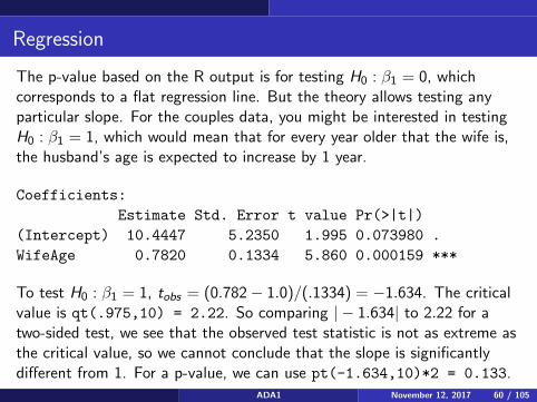
Regression

The p-value based on the R output is for testing H0 : β1 = 0, whichcorresponds to a flat regression line. But the theory allows testing anyparticular slope. For the couples data, you might be interested in testingH0 : β1 = 1, which would mean that for every year older that the wife is,the husband’s age is expected to increase by 1 year.

Coefficients:

Estimate Std. Error t value Pr(>|t|)

(Intercept) 10.4447 5.2350 1.995 0.073980 .

WifeAge 0.7820 0.1334 5.860 0.000159 ***

To test H0 : β1 = 1, tobs = (0.782− 1.0)/(.1334) = −1.634. The criticalvalue is qt(.975,10) = 2.22. So comparing | − 1.634| to 2.22 for atwo-sided test, we see that the observed test statistic is not as extreme asthe critical value, so we cannot conclude that the slope is significantlydifferent from 1. For a p-value, we can use pt(-1.634,10)*2 = 0.133.

ADA1 November 12, 2017 60 / 105

Regression

Instead of getting values such as the SE by hand from the R output, youcan also save the output to a variable and extract the values. This reducesroundoff error and makes it easier to repeat the analysis in case the datachanges. For example, from the previous example, we could use

model1.values <- summary(model1)

b1 <- model1.values$coefficients[2,1]

b1

#[1] 0.781959

se.b1 <- model1.values$coefficients[2,2]

t <- (b1-1)/se.b1

t

#[1] -1.633918

The object model1.values$coefficients here is a matrix object, so thevalues can be obtained from the rows and columns.

ADA1 November 12, 2017 61 / 105

Regression

For the CI for this example, we have

df <- model1.values$fstatistic[3] # this is hard to find

t.crit <- qt(1-0.05/2, df)

CI.lower <- b1 - t.crit * se.b1

CI.upper <- b1 + t.crit * se.b1

print(c(CI.lower,CI.upper))

#[1] 0.4846212 1.0792968

Consistent with the hypothesis test, the CI includes 1.0, suggesting wecan’t be confident that the ages of husbands increase at a different ratefrom the ages of their wives.

ADA1 November 12, 2017 62 / 105

Regression

As mentioned earlier, the R output tests H0 : β1 = 0, so you need toextract information to do a different test for the slope. We showed using at-test for testing this null hypothesis, but it is also equivalent to an F test.Here the F statistic is t2obs when there is only 1 numerator degree offreedom (one predictor in the regression).

t <- (b1-0)/se.b1

t

#[1] 5.859709

t^2

#[1] 34.33619

which matches the F statistic from earlier output.

In addition, the p-value matches that for the correlation usingcor.test(). Generally, the correlation will be significant if and only if theslope is signficantly different from 0.

ADA1 November 12, 2017 63 / 105

Regression

Another common application of confidence intervals in regression is for theregression line itself. This means getting a confidence interval for theexpected value of y for each value of x .Here the CI for y given x is

b0 + b1x ± tcritsY |X

√1

n+

(x − x)2∑i (xi − x)2

where the critical value is based on n − 2 degrees of freedom.

ADA1 November 12, 2017 64 / 105

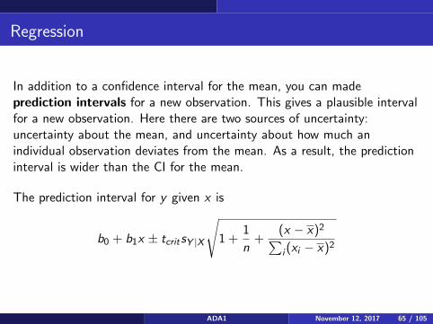
Regression

In addition to a confidence interval for the mean, you can madeprediction intervals for a new observation. This gives a plausible intervalfor a new observation. Here there are two sources of uncertainty:uncertainty about the mean, and uncertainty about how much anindividual observation deviates from the mean. As a result, the predictioninterval is wider than the CI for the mean.

The prediction interval for y given x is

b0 + b1x ± tcritsY |X

√1 +

1

n+

(x − x)2∑i (xi − x)2

ADA1 November 12, 2017 65 / 105

Regression

For a particular wife age, such as 40, the CIs and PIs (prediction intervals)are done in R by

predict(model1,data.frame(WifeAge=40), interval="confidence",

level=.95)

# fit lwr upr

#1 41.72307 38.30368 45.14245

predict(model1,data.frame(WifeAge=40), interval="prediction",

level=.95)

# fit lwr upr

#1 41.72307 29.6482 53.79794

Here the predicted husband’s age for a 40-yr old wife is 41.7 years. A CI for the

mean age for the husband is (38.3,45.1), but a prediction interval is that 95% of

husbands for a wife this age would be between 29.6 and 53.8 years old. There is

quite a bit more uncertainty for an individual compared to the population

average.ADA1 November 12, 2017 66 / 105

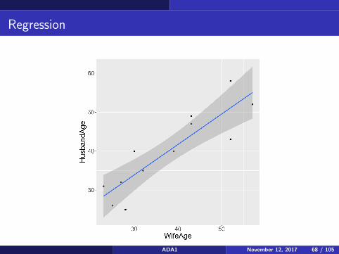
Regression

To plot the CIs at each point, here is some R code:

library(ggplot2)

p <- ggplot(x, aes(x = WifeAge, y = HusbandAge))

p <- p + geom_point()

p <- p + geom_smooth(method = lm, se = TRUE)

p <- p + theme(text = element_text(size=20))

print(p)

ADA1 November 12, 2017 67 / 105

Regression

ADA1 November 12, 2017 68 / 105

Regression

Note that the confidence bands are narrow in the middle of the data. Thisis how these bands usually look. There is less uncertainty near the middleof the data than there is for more extreme values. You can also see this inthe formula for the SE, which has (x − x)2 inside the square root. This isthe only place where x occurs by itself. The further it is from x , the largerthis value is, and therefore the larger the SE is.

ADA1 November 12, 2017 69 / 105

Regression

There is a large literature on regression diagnostics. This involves checkingthe assumptions of the regression model. Some of the most importantassumptions, such as that observations are independent observations froma single population (e.g., the population of married couples), cannot bechecked just by looking at the data. Consequently, regression diagnosticsoften focus on what can be checked by looking at the data.

To review, the model is yi = β0 + β1xi + εi where

1. the observed data are a random sample

2. the average y value is linearly related to x

3. the variation in y given x is independent of x (the variability is thesame for each level of x

4. the distribution of responses for each x is normally distributed withmean β0 + β1x (which means that ε is normal with mean 0)

ADA1 November 12, 2017 70 / 105

Regression

The following plots show examples of what can happen in scatterplots:

(a) Model assumptions appear to be satisfied

(b) The relationship appears linear, but the variance appears nonconstant

(c) The relationship appears nonlinear, althought the variance is appearsto be constant

(d) The relationship is nonlinear and the variance is not constant

ADA1 November 12, 2017 71 / 105

Regression

ADA1 November 12, 2017 72 / 105

Regression

ADA1 November 12, 2017 73 / 105

Regression

Regression diagnostics are often based on examinging the residuals:

ei = yi − yi = yi − (b0 + b1xi )

Based on the model assumptions, the residuals should be normallydistributed with mean 0 and some variance σ2. To standardize theresiduals, they are often divided by their standard error. Here ri is calledthe studentized residual:

ri =ei

SE (ei )=

ei

sY |X

√1n + (xi−x)2∑

i (xi−x)2

ADA1 November 12, 2017 74 / 105

Regression

The studentized residuals are standard normal (if the model is correct), somost studentized residuals should be between -2 and +2, just like z-scores.Often studentized residuals are plotted against the fitted values, yi .

For this plot, there is no trend, and you should observed constant varianceand no obvious patterns like U-shapes.

ADA1 November 12, 2017 75 / 105

Regression

Good residual plot.

ADA1 November 12, 2017 76 / 105

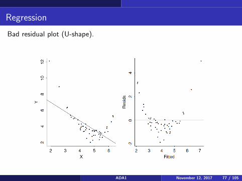
Regression

Bad residual plot (U-shape).

ADA1 November 12, 2017 77 / 105

Regression

Residual plot with extreme outlier.

ADA1 November 12, 2017 78 / 105

Typing plot(model1) (or whatever the name of your model from lm())and then return several times, R will plot several diagnostic plots. The firstis the residuals (not studentized) against the fitted values. This help youlook for outliers, nonconstant variance and curvature in the residuals.

ADA1 November 12, 2017 79 / 105

Regression

Another type of residual is the externally Studentized residual (also calledStudentized deleted residual or deleted t-residual), which is based onrerunning the analysis without the ith observation, then determining whatthe difference would be between yi and b0 + b1xi , where b0 and b1 areestimated with the pair (xi , yi ) removed from the model. This could bedone by tediously refitting the regression model n times for n pairs of data,but this can also be done automatically in the software, and there arecomputational ways to make it reasonably efficient.

The point of doing this is that if an observation is outlier, it might have alarge influence on the regression line, making its residual not as extreme asif the regression was fit without the line. The Studentized deleted residualsgive a way of seeing which observations have the biggest impact on theregression line. If the model assumptions are correct (without extremeoutliers), then the Studentized deleted residual has a t distribution withn − 2 degrees of freedom.

ADA1 November 12, 2017 80 / 105

Regression

Something to be careful of is that if you have different numbers ofobservations for different values of x , then larger sample sizes will naturallyhave a larger range. Visually, this can be difficult to distinguish fromnonconstant variance. The following examples are simulated.

ADA1 November 12, 2017 81 / 105

Regression


ADA1 November 12, 2017 82 / 105

Regression


ADA1 November 12, 2017 83 / 105

Regression


ADA1 November 12, 2017 84 / 105

Regression


ADA1 November 12, 2017 85 / 105

Regression

The normality assumption for regression is that the responses are normallydistributed for each level of the predictor. Note that it is not assumed thatthe predictor follows any particular distribution. The predictor can benonnormal, and can be chosen by the investigator in the case ofexperimental data. In medical data, the investigator might recruitindividuals based on their predictors (for example, to get a certain agegroup), and then think of the response as random.

It is difficult to tell if the responses are really normal for each level of thepredictor, especially if there is only one response for each x value (whichhappens frequently). However, the model also predicts that the residualsare normally distributed with mean 0 and constant variance. The indvidualvalues yi come from different distributions (because they have differentmeans), but the residuals all come from the same distribution according tothe model. Consequently, you can check for normality of the residuals.

ADA1 November 12, 2017 86 / 105

Regression

As an example, the QQ plot is also generated by typing plot(model1) andhitting return several times. The command plot(model1) will generatefour plots. To see them all you might type par(mfrow=c(2,2)) to putthem in a 2× 2 array first. You can also do a formal test on the residuals

par(mfrow=c(2,2))

plot(model1)

shapiro.test(model1$residual)

# Shapiro-Wilk normality test

#

#data: model1$residual

#W = 0.95602, p-value = 0.7258

ADA1 November 12, 2017 87 / 105

QQ plot

ADA1 November 12, 2017 88 / 105

Regression

Studentized residuals, i.e., residuals divided by their standard errors so thatthey look like z-scores, can be obtained from R using rstudent(model1).It helps to sort them to see which ones are most extreme.

rstudent(model1)

sort(rstudent(model1))

# 7 2 10 4 11 12

#-2.02038876 -1.65316857 -0.83992238 -0.69122350 -0.17987025 -0.09016353

# 6 9 8 1 3 5

# 0.08799631 0.54099532 0.57506585 1.00173208 1.29257824 1.61935539

ADA1 November 12, 2017 89 / 105

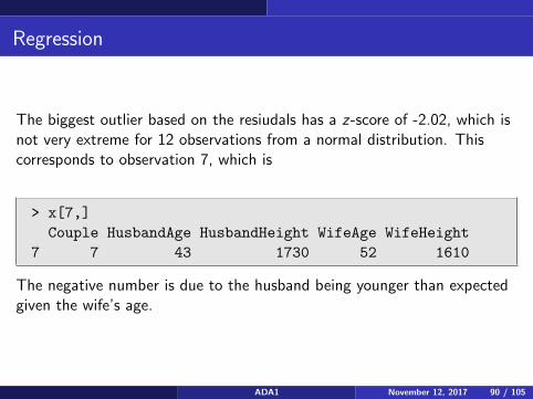
Regression

The biggest outlier based on the resiudals has a z-score of -2.02, which isnot very extreme for 12 observations from a normal distribution. Thiscorresponds to observation 7, which is

> x[7,]


7 7 43 1730 52 1610

The negative number is due to the husband being younger than expectedgiven the wife’s age.

ADA1 November 12, 2017 90 / 105

Regression

If there are outliers in the data, you have to be careful about how toanalyze them. If an outlier is due to an incorrect measurement or error inthe data entry, then it makes sense to remove it. For a data entry error,you might be able to correct the entry by consulting with the investigators,for example if a decimal is put in the wrong place. This is preferable tosimply removing the data altogether.

If an outlier corresponds to genuine data but is removed, I would typicallyanalyze the data both with and without the outlier to see how much of adifference it makes. In some cases, keeping an outlier might not changeconclusions in the model. Removing the outlier will tend to decreasevariability in the data, which might make you underestimate variances andstandard errors, and therefore incorrect conclude that you have signficanceor greater evidence than you actually have.

ADA1 November 12, 2017 91 / 105

Regression

Removing an outlier that is a genuine observation also makes it less clearwhat population your sample represents. For the husband and wifeexample, if we removed a couple that appeared to be an outlier, we wouldbe making inferences about the population of couples that do not haveunusual ages or age combinations, rather than inferences about the moregeneral population, which might include unusual ages.

ADA1 November 12, 2017 92 / 105

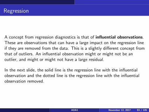
Regression

A concept from regression diagnostics is that of influential observations.These are observations that can have a large impact on the regression lineif they are removed from the data. This is a slightly different concept fromthat of outliers. An influential observation might or might not be anoutlier, and might or might not have a large residual.

In the next slide, the solid line is the regression line with the influentialobservation and the dotted line is the regression line with the influentialobservation removed.

ADA1 November 12, 2017 93 / 105

Regression

ADA1 November 12, 2017 94 / 105

Regression

Note that in the previous slide, the left plot has an observation with anunusal y value, but that the x value for this observation is not unusual.For the right plot, the outlier is unusual in both x and y values.

Typically, an unusual x value has more potential to greatly alter theregression line, so a measure called influence has been developed based onhow unusual an observation is in the predictor variable(s), without takinginto account the y variable.

ADA1 November 12, 2017 95 / 105

Regression

To see measures of influence, you can type influence(model1), wheremodel1 is whatever you saved your lm() call to. The leverage valuesthemselves are obtained by influence(model1)$hat. Leverages arebetween 0 and 1, where values greater than about 2p/n or 3p/n, where pis the number of predictors, are considered large. If 3p/n is greater than 1,you can use 0.99 as a cutoff.

> influence(model1)$hat

> influence(model1)$hat

1 2 3 4 5 6 7 8

0.1027 0.1439 0.1212 0.3319 0.2203 0.1572 0.2203 0.1027

9 10 11 12

0.2235 0.1877 0.0847 0.1039

ADA1 November 12, 2017 96 / 105

Regression

For the husband and wife age data, observation 4 has the highest leverage,and this corresponds to the couple with the highest age for the wife.Recall that for leverage, the y variable (husband’s age) is not used.However, the value here is 0.33, which is not high for leverages. Recallthat the observation with the greatest residual was observation 7.

> x[4,]


4 4 52 1779 57 1540

ADA1 November 12, 2017 97 / 105

Regression

The formula for the leverage is somewhat complicated (it is usually definedin terms of matrices), but to give some intuition, note that the z-scores forthe wife’s ages also give observation 4 as the most unusual, with a z-scoreof 1.65:

> (x$WifeAge-mean(x$WifeAge))/sd(x$WifeAge)

[1] 0.461 -0.816 -0.646 1.653 1.228 -0.901 1.228

0.461 -1.242 -1.072 0.121 -0.475

ADA1 November 12, 2017 98 / 105

Regression

Another measure of influence is Cook’s distance or Cook’s D. Anexpression for Cook’s D is

Dj ∝∑i

(yi − yi [−j])2

Here yi [−j] is the predicted value of the ith observation when theregression line is computed with the jth observation removed from thedata set. This statistic is based on the idea of recomputing the regressionline n times, each time removing observation j , j = 1, . . . , n to get astatistic for how much removing the jth observation changes theregression line for the remaining.

The symbol ∝ means that the actual value is a multiple of the value thatdoesn’t depend on j . There are different interpretations for what counts asa large value of Dj . One is values of Dj > 1. Another approach is to see ifDj is large for some j compared to other Cook’s distances in the data.

ADA1 November 12, 2017 99 / 105

Regression

> cooks.distance(model1)

1 2 3 4 5 6

0.057390 0.195728 0.108014 0.125200 0.318839 0.000802

7 8 9 10 11 12

0.440936 0.020277 0.045336 0.083990 0.001656 0.000523

ADA1 November 12, 2017 100 / 105

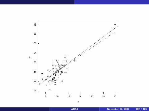
Regression

Cook’s distance depend’s on an observation being unusual for both x andy and having an influence on the regression line. In this case, observation7 has the highest Cook’s D, but it is not alarming. In the followingexample, an artificial data set with 101 observations has an outlier that isfairly consistent with the overall trend of the data with the outlierremoved. However, Cook’s D still picks out the outlier. As before, thesolid line is with the outlier included.

ADA1 November 12, 2017 101 / 105

ADA1 November 12, 2017 102 / 105

Regression

a <- lm(y ~ x)

hist(cooks.distance(a))

ADA1 November 12, 2017 103 / 105

Regression

Note that with one predictor we can pretty easily plot the data andvisually see unusual observations. In multiple dimensions, with multiplepredictor variables, this becomes more difficult, which makes thesediagnostic techniques more valuable when there are multiple predictors.This will be explored more next semester.

The following is a summary for analyzing regression data.

ADA1 November 12, 2017 104 / 105

Regression

1. Plot the data. With multiple predictors, a scatterplot matrix is theeasiest way to do this.

2. Consider transformations of the data, such as logarithms. For countdata, square roots are often used. Different transformations will beexplored more next semester.

3. Fit the model, for example using aov() or lm()

4. Examine residual plots. Here you can look forI curvature in the residuals or other nonrandom patternsI nonconstant varianceI outliersI normality of residuals

ADA1 November 12, 2017 105 / 105

Regression

5. Check Cook’s D values

6. If there are outliers or influential observations, consider redoing theanalysis with problematic points removed

ADA1 November 12, 2017 106 / 105

Documents

ADA1: Chapter8, Correlation & Regressionjames/chapter8f.pdf · Chapter 8: Correlation & Regression ADA1 November 12, 2017 13 / 105. Chapter 8: Correlation & Regression ADA1 November