AD-A259 EIIhIIhIIIIIfIIIIIIUI · AD-A259 EIIhIIhIIIIIfIIIIIIUI 076 f ... expertise and valuable insight. ... Delta coefficients using an approx-imate 100 msec window (± 8 frames)

AD-A259 076EIIhIIhIIIIIfIIIIIIUI fAFIT/GE/ENG/92D-11

CEPSTRAL AND AUDITORY MODEL FEATURES

FOR SPEAKER RECOGNITION

THESISJohn M. Colombi

Captain, USAF DTICAFIT/GE/ENG/92D-11 EL ECTF

190

Approved for public release; distribution unlimited

93 1 04 151

AFIT/GE/ENG/92D-11

CEPSTRAL AND AUDITORY MODEL FEATURES FOR SPEAKER

RECOGNITION

THESIS

Presented to the Faculty of the School of Engineering

of the Air Force Institute of Technology

Air University

In Partial Fulfillment of the

Requirements for the Degree of

Master of Science in Electrical Engineering

Aoesslon For

NTIS GRA&IDTIfl TAB 0Uni-ruio t•nced El

John M. Colombi, B.S.E.E.Captain, USAF By___

DIstribution/

Avallab 111ty CodesiAvail and/or

Dist SpelalDecember 1, 1992

Approved for public release; distribution unlimited

Acknowledgments

I wish to thank my thesis committee with their diverse backgrounds and individual

contributions. Individual thanks to Dr. Steven Rogers for his unique approach and guid-

ance. It has been said he expects and demands nothing ... but best from you. I truly

enjoyed the material within this thesis, thanks to him. I must personally give thanks to

Dr. Tim Anderson whose expertise on auditory models and whose frequent discussions

and daily interactions made this thesis a pleasure. His computer and disk resources, and

my allowed control over them, were invaluable. Thanks also to the other professors who

lent consideration, expertise and valuable insight. I must finally thank my (usually un-

derstanding) wife Cheryl, who managed to juggle work, school and two adorable children.

She will always be my inspiration.

John M. Colombi

Table of Contents

Page

Acknowledgments .......... .................................... 1i

Table of Contents ........... .................................... ii

List of Figures .......... ...................................... vi

List of Tables .......... ....................................... ix

Abstract .......... .......................................... Xi

I. Introduction ............................................. 1

1.1 Background ...................................... 1

1.2 Problem ......................................... 1

1.3 Assumptions ......... ............................. 2

1.4 Scope ......... ................................. 2

1.5 Approach /Methodology .............................. 2

1.6 Conclusion ......... .............................. 3

II. Literature Review ......... ................................ 4

2.1 Introduction ........ ............................. 4

2.2 Feature Extraction ........ ......................... 5

2.2.1 Linear Prediction Analysis ..................... 8

2.2.2 Cepstrum Analysis ...... .................... 8

2.3 Classification and Clustering ........................... 16

2.3.1 Vector Quantization and Distortion Based Classification 17

2.3.2 Hidden Markov Models/ Gaussian Models ............ 31

2.3.3 Artificial Neural Network Classification ............. 34

iii

Page

2.4 Payton Model of the Mammalian Auditory System ........... 36

2.4.1 Stage 1/ Middle Ear ........................... 38

2.4.2 Stage 2/ Basilar Membrane ...................... 38

2.4.3 Stage 2 Comparisons ........................... 44

2.4.4 Stage 3/Inner Hair Cell Transduction/ Synapse . . .. 45

2.4.5 Stage 3 Comparisons ........................... 48

2.4.6 Payton Analysis ............................. 50

2.5 Conclusion ......... .............................. 51

III. Methodology .......... ................................... 53

3.1 Introduction ......... ............................. 53

3.2 Feature Extraction .................................. 54

3.2.1 LPC Cepstral ....... ....................... 55

3.2.2 Payton Model ............................... 57

3.3 Clustering Methodology .............................. 59

3.3.1 LBG Design ................................ 62

3.3.2 Kohonen Design ............................. 65

3.3.3 Fusion Techniques ............................ 67

3.4 Conclusion ......... .............................. 70

IV. Experimentation/ Results ........ ............................ 71

4.1 TIMIT Experimentation .............................. 71

4.2 KING Experimentation .............................. 73

4.2.1 10 Class Tests ....... ....................... 73

4.2.2 26 Class Tests ....... ....................... 76

4.2.3 Fusion Results .............................. 78

4.2.4 Speaker Verification ........................... 79

4.2.5 Feature Analysis ............................. 79

iv

Page

4.3 AFIT Corpus Experimentation ......................... 83

4.3.1 Recording Setup ............................. 83

4.3.2 Recognition Results ....... .................... 83

4.4 Conclusion ........ .............................. 85

V. Conclusions/ Final Analysis ................................... 87

5.1 Quantization Design/ Classification .................... .87

5.2 Preprocessing ......... ............................ 89

5.3 Auditory Modeling .................................. 90

Appendix A. Human Auditory Physiology ........................... 93

A.1 Human Physiology .................................. 93

A.2 Peripheral Functionality/ Quantitative Analysis ............. 95

A.2.1 Frequency Selectivity ........................ .98

A.2.2 Phase Synchrony ............................. 99

A.2.3 Spontaneous Rate and Thresholds ................. 102

A.2.4 Nerve Firing Functionality ...................... 103

Vita ........... ............................................ 104

Bibliography .......... ....................................... 105

v

List of Figures

Figure Page

1. Sample Speech (Vowel IY, male speaker) ....... .................. 10

2. Sample Spectrum. The previous samples correspond to the first voiced region,

at approximately 0.2 sec ........ ............................. 10

3. Sample 8th order Power Cepstrum (128 coefficients) of the referenced voiced

samples. The plot shows consecutive 16 msec frames calculated every 5.33

msec during the phoneme IY ........ .......................... 11

4. Mel Frequency Scale [80] ........ ............................ 12

5. 20th order LPC Cepstral using. Note pertinent spectral shape information of

the power cepstrum. The plot shows consecutive 16 msec frames calculated

every 5.33 msec during the phoneme IY ....... .................... 15

6. Speaker Recognition Classification Paradigms ...................... 20

7. Kohonen 2D Lattice ......... ............................... 25

8. Composite Payton Auditory Model ............................. 39

9. Original sampled data from the TIMIT database, scaled by 8000. The sen-

tence (male speaker) reads,"She had your dark suit in greasy wash water all

year.. .......... ....................................... 40

10. Original sentence after First Stage of Payton Model. Sound pressure (sampled

speech data) is converted to stapes velocity (microns/sec) .............. 40

11. Uncoiled Cochlea Model ........ ............................. 42

12. Original sentence through the Basilar Membrane Second Stage of Payton

Model, but before second filter sharpening - Phoneme [IY] .............. 42

13. Original sentence through Basilar Membrane Sharpening Mechanism, a sec-

ond filter with a zero placed below, and a pole placed just above the charac-

teristic frequency - Phoneme [IY] ............................... 44

14. Neural Firing Range ........ ............................... 46

15. Payton implementation of Brachman (1980) Reservoir Scheme of "Neuro-

transmitter" release ........................................ 47

vi

Figure Page

16. Original sentence after Final Transduction Stage of Payton Model - Phoneme

[IY] .............................................. 48

17. Original sentence Spectogram, using 256 point DFT, window size 16 msec.

frame rate 5.33 msec ........ ............................... 49

18. Original sentence after Final Transduction Stage of Payton Model, averaged

with a window size of 16 msec and a frame rate 5.33 msec .............. 49

19. Preemphasis Filter ......... ................................ 55

20. Four Speakers Distortion with varying codebooks, using TIMIT vowels. .. 60

21. Vowel and Non-Silence Tests .................................. 61

22. TIMIT speaker "mcmj" utterance showing distortions to all speaker depen-

dent codebooks (LBG) using all speech. Note the low Figure of Merit for the

winning codebook ......................................... 63

23. TIMIT speaker "mcmj" utterance showing distortions to all speaker depen-

dent codebooks (LBG) using vowels. Note the higher Figure of Merit for the

winning codebook ......................................... 63

24. Gaussian Data Source, p = (0, 0) and a = 0.5 ...................... 64

25. LBG Algorithm Quantizer Design, 1 to 8 codebooks, I = (0, 0) and a = 0.5. 64

26. LBG Algorithm Quantizer Design, Final 64 codebooks, Y = (0, 0) and a =

0.5. Quantization SNR = 15.5 dB ............................... 65

27. Kohonen learning for a TIMIT male(M) and female(F) speaker for varying

iterations (epochs) for LPC cepstral and also Payton. Quantizer "learns" in

the first 100 epochs then stabilizes .............................. 66

28. Kohonen learning schedule ........ ........................... 66

29. Kohonen Learning Algorithm run for 100 epochs, 64 codewords, for a single

2D gaussian with u = (0,0) and a = .5. Quantization SNR = 11.13dB . . . 67

30. Same as Figure 29 with DeSieno conscience, conscience parameters B and C

were .0001 and .1 respectively, for a single 2D gaussian with i = (0, 0) and

a = .5. Quantization SNR = 11.32dB ............................. 68

31. Kohonen / Competitive learning, 64 codewords, for a single 2D gaussian with

p = (0, 0) and a = .5.. Quantization SNR = 15.93dB ................. 68

vii

Figure Page

32. Recognition Performance of TIMIT LPC cepstral ...... .............. 72

33. KING Database: Speaker Recognition using delta Payton auditory model

coefficients. Shown are Competitive learning and LBG on both Payton ajid

Payton zero-mean normalization; 10 speakers ...................... 76

34. Cepstral Speaker Separability ................................. 83

35. Payton Speaker Separability ........ .......................... 83

36. Recognition over increasing training sessions for the AFIT corpus ...... .. 85

37. Verification Error over increasing training sessions for the AFIT corpus using

cepstral coefficients ........................................ 85

38. Human Auditory Periphery, showing outer ear, middle ear and inner ear

cavities [120] ......... ................................... 94

39. Cochlear Partitions [120] ........ ............................ 95

40. Internal Structures of the Scala Media [1201 ........................ 96

41. Auditory Tuning Curve ...................................... 99

42. Neuron Characteristic Frequency Selectivity 1 ...................... 100

43. Neuron Characteristic Frequency Selectivity 2. Note the non-linear distortion

at high signal intensities ..................................... 101

44. Neural InterSpike Histograms ................................. 102

viii

List of Tables

Table Page

1. Feature Extraction Examples for Speaker Recognition ................. 6

1. (cont'd) Feature Extraction Examples for Speaker Recognition ........ 7

2. Classification Techniques for Speaker Recognition ..... .............. 18

2. (cont'd) Classification Techniques for Speaker Recognition ............. 19

3. Several Auditory Models and their Features ........................ 37

4. Characteristic Frequency of Payton Model 20 Channels.[4] ............. 43

5. TIMIT Energy Characteristics ........ ......................... 58

6. KING Energy Characteristic; Average taken over sessions 1 - 5 ....... ... 59

7. TIMIT comparison of quantization distortions. TRAINING refers to the sal

and sa2 sentences, TEST refers to averaged sx sentences ............... 62

8. TIMIT Database: Speaker classification. Trained on sal and sa2, tested on

sx ........... .......................................... 72

9. TIMIT Database: Speaker classification. Trained on sal and sa2, tested on

sx with 10dB AWGN ....................................... 73

10. TIMIT Database: Speaker classification. Delta coefficients using an approx-

imate 100 msec window (± 8 frames). Trained on sal and sa2, tested on

SX ............................. .......................................... 73

11. KING Database: Speaker classification. Trained on sessions 1 - 3, tested on

sessions 4 and 5; 10 speakers .................................. 74


sessions 4 and 5, Kohonen Modifications; 10 speakers ................. 74


sessions 4 and 5. Probability of Voicing Influence on the Payton Model; 10

speakers .......... ...................................... 75


sessions 4 and 5. Normalization Influence on the Payton Model ....... ... 75


sessions 4 and 5. Kohonen Training Time Influence on the Payton Model.. 75

ix

Table Page

16. KING Database- Speaker classification. Delta cepstral coefficients using an

approximate 100 msec window (± 4 frames), with various normalization.

Trained on sessions 1 - 3, tested on sessions 4 and 5; 10 speakers ....... 77


sessions 4 and 5. Cepstral Normalization and BandPass Liftering procedures;

10 speakers .......... .................................... 77


sessions 4 and 5. Effects of 15 low Characteristic Frequency Payton coeffi-

cients; 10 speakers ......................................... 77


sessions 4 and 5. Effects of ALL San Diego speakers ................... 78


sessions 4 and 5. Effects of number of cepstral coefficients; 26 speakers. .. 78

21. KING Database: Speaker classification. Average and Figure of Merit (FOM)

Fusion. Note - PAM is Payton Auditory Model, LPCC is LPC cepstral and

(0) represents zero mean normalization; 10 speakers ................... 80

22. KING Database: Speaker classification. Average, Figure of Merit (FOM)

and Weighted Fusion. Note - PAM is Payton Auditory Model, LPCC is

LPC cepstral and (0) represents zero mean normalization. WEIGHTED uses

the recognition accuracy of the individual classifiers for weights in fusion; 10

speakers .......... ...................................... 80

23. KING Database: Speaker classification. Average and Figure of Merit (FOM)

Fusion. Note - PAM is Payton Auditory Model, LPCC is LPC cepstral and

(0) represents zero mean normalization; 26 speakers ................... 80

24. KING Database: Speaker Authentication. Trained on sessions 1 - 3, tested

on sessions 4 and 5; 13 Targer speakers, 13 Imposters ................. 80

25. KING Database: Speaker dependent codebook evaluation with Fisher Ratio

[801 ............ ........................................ 81

26. AFIT User Identification Database: Speaker Identification using Phonetically

Balanced and Speaker Names ......... ........................ 84

27. AFIT User Identification Database: Speaker Identification using other names. 84

x

AFIT/GE/ENG/92D- 11

Abstract

The TIMIT and KING databases, as well as a ten day AFIT speaker corpus, are used

to compare proven spectral processing techniques to an auditory neural representation for

speaker identification. The feature sets compared were Linear Predictive Coding (LPC)

cepstral coefficients and auditory nerve firing rates using the Payton model. This auditory

model provides for the mechanisms found in the human middle and inner auditory periph-

ery as well as neural transduction. Clistering algorithms were used successfully to generate

speaker specific codebooks - one statistically based and the other a neural approach. These

algorithms are the Linde-Buzo-Gray (LBG) algorithm and a Kohonen self-organizing fea-

ture map (SOFM). The LBG algorithm consistently provided optimal codebook designs

with corresponding better classification rates. The resulting Vector Quantized (VQ) distor-

tion based classification indicates the auditory model provides slightly reduced recognition

in clean studio quality recordings (LPC 100%, Payton 90%), yet achieves similar perfor-

mance to the LPC cepstral representation in both degraded environments (both 95%) and

in test data recorded over multiple sessions (both over 98%). A variety of normalization

techniques, preprocessing procedures and classifier fusion methods were examined on this

biologically motivated feature set.

This thesis provides the first comparative analysis between conventional signal pro-

cessing and nenral representations on the same speaker utterances. It also provides the

first classification results using a speaker corpus of ,ion-st- bio quality, specifically KING.

Lastly, the effects of multiple session training time for speaker r* cognition using an auditory

model is precedent.

xi

CEPSTRAL AND AUDITORY MODEL FEATURES FOR SPEAKER

RECOGNITION

I. Introduction

1.1 Background

Accurate and robust speech recognition has evaded researchers for over four decades.

The ability to effortlessly communicate with our growing computer environment has at-

tracted a large body of research internationally. One particular aspect of this problem is

automatic speaker recognition (ASR). Speaker recognition is defined as the ability to rec-

ognize individuals only by the received acoustic speech signal. The technologies which sup-

port this goal would allow identification or verification of individuals in such applications

as DoD surveillance, forensic data, and secure facility access. Adaptation to individual

speech patterns may also prove useful in improved speech processing.

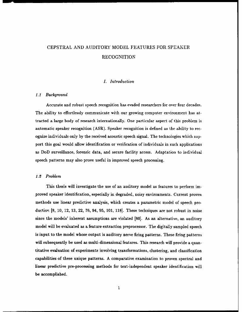
1.2 Problem

This thesis will investigate the use of an auditory model as features to perform im-

proved speaker identification, especially in degraded, noisy environments. Current proven

methods use linear predictive analysis, which creates a parametric model of speech pro-

duction [8, 10, 12, 13, 22, 76, 94, 95, 101, 118]. These techniques are not robust in noise

since the models' inherent assumptions are violated [80]. As an alternative, an auditory

model will be evaluated as a feature extraction preprocessor. The digitally sampled speech

is input to the model whose output is auditory nerve firing patterns. These firing patterns

will subsequently be used as multi-dimensional features. This research will provide a quan-

titative evaluation of experiments involving transformations, clustering, and classification

capabilities of these unique patterns. A comparative examination to proven spectral and

linear predictive pre-processing methods for text-independent speaker identification will

be accomplished.

1.3 Assumptions

The hypothesis which underlies this rescarch ib that an auditory neural representa-

tion contains speaker dependent information, either instantaneously or through temporal

patterns, as well as providing adequate resolution of this information. The human audi-

tory system performs both types of processing. The cochlea encodes received information

based on frequency analysis (frequency or place theory) as well as temporal patterns of

the stimulus (temporal theory) [70, 71]. This is accomplished by the location of neurons

along the basilar membrane as well as the synchronization of their firing. Current methods

of speaker identification often perform a linear predictive analysis on the speech signal.

This process fits a linear all-pole model to the speech production [67, 80]. However, this

model, which accounts for the speakers' vocal tract and other speech production apparatus

is directly speaker dependent. The frequency analysis capabilities of the auditory model

may not contain the necessary resolution for speaker dependence.

1.4 Scope

The TIMIT and KING databases, as well as an AFIT recorded corpus, are used to

compare and analyze proven spectral processing techniques to an auditory neural represen-

tation for speaker recognition. The primary contribution provides measures of an auditory

model representation to contain speaker dependent information. The ability of these fea-

tures to generalize for added noise and intra-speaker distortions will be experimentally

evaluated.

1.5 Approach /Methodology

This thesis initially investigates popular Linear Predictive Coding (LPC) Cepstral

processing on the DARPA TIMIT Phonetic Speech Database. Various Vector Quantization

(VQ) classification techniques were evaluated to create a c, .antitative baseline. Varying

degrees of additive white Gaussian noise added to the speech utterance were incorporated

in this baseline. An auditory model proposed by Payton will be used to extract audi-

tory nerve firing rates with the same VQ distortion metrics used for classification. These

quantizers include the recursive Linde-Buzo-Gray splitting technique and various configu-

2

rations of Kohonen's Self Organizing Feature Maps. This research will use the hypothesis

that long-term averages of the short-term spectrum contain speaker dependent information

[113]. Experimentation will investigate various temporal characteristics [1141 of the speech

signal using a simple difference procedure [56]. Lastly, classification fusion techniques will

determine correlation of classification errors between the various features. These results

will determine the measure of speaker dependent information of a neural auditory model, in

conjunction with clustering analysis and artificial neural networks, to improve performance

of speaker identification.

1.6 Conclusion

This thesis will first provide the significant background on this multifaceted prob-

lem. Speech and speaker recognition can include such diversive areas as signal processing,

linear modeling and mathematics, physiological and psychological theories, biology, and

pattern analysis. Chapter II provides an historic synopsis of key techniques examined,

with a major source of information extracted from the recent International Conference of

Acoustics, Speech and Signal Processing (ICASSP) proceedings. The chapter will exam-

ine the analysis of feature extraction by spectral and linear processing models, summarize

vector quantization techniques and their related distortion based classification metrics for

speaker identification, and lastly detail the Payton auditory model. Methodology, experi-

mentation and results are contained in Chapters III and IV. Chapter V provides pertinent

conclusions and analysis. For additional information on the human auditory periphery and

its quantitative analysis, refer to Appendix A.

3

IL Literature Review

2.1 Introduction

Automatic Speaker Recognition (ASR) is one of many emerging technologies which

will support an effortless and natural interaction with the growing computer environment.

Though many techniques have publicized remarkable accuracies, they are typically limited

by size of speaker populations, small vocabularies or restricted sentences, and noise-free

environments (see Table 2). One model which may overcome the current limitations in

noise of speaker recognizers is based on the human auditory system; such models have

demonstrated improvements for speech recognition [5, 7, 37, 38]. This review examines the

achievements in Automatic Speaker Recognition.

Speaker recognition is often defined in two separate categories: speaker verification

(authentication) and speaker identification. Verification, the easier of the two, is a process

whereby a recognizer provides a decision to accept or dens a claim of identity by an

unknown individual. This is attempted solely by analysis of a speech utterance, either

specific text (text-dependent) or non-prompted (text-independent) speech. Identification

is the process of choosing the identity from a known population of many speakers; as well as

responding appropriately to an unknown individual not contained in this set. This review

will clarify the multiple classification and clustering techniques, as well as detail some of

the current features extracted from the speech signal.

In a recent I.E.E.E. Proceedings article, C. Weinstein discusses the opportunities for

advanced military applications based on speech technologies. These opportunities include

military security, advanced battle management, advanced pilot cockpits and improved air

traffic control training [1211. He states that current speaker recognition research is focusing

on the difficult text-independent problem, with the goal of achieving higher performance in

noise and communications channel degradation. Others point out that biometric features

such as fingerprints, hand geometry, or retinal images can be recognized, as well as an

individual's unique activities, such as handwriting, keyboard typing, or speech [72]. Results

have also been reported on recognition of individuals by their face images [116, 119].

Speaker recognition can also be directly applied to speaker selection or adaptation, so as

4

to improve speech recognition techniques [32]. Lastly, it has been said that humans are

unable to appreciate the difficulties that speaker recognition poses for a computer, since

humans comprehend speech so easily [58].

First, this review will discuss the various features often extracted from the speech sig-

nal. In the following sections, details on the current classification and clustering paradigms

will be presented, focusing on vector quantization (VQ) techniques and including the

popular Hidden Markov Model and Artificial Neural Networks (connectionist) paradigms.

Lastly, some recent representations using auditory models for speech recognition and de-

tails concerning the Payton model are examined.

2.2 Feature Extraction

A tight coupling exists between a feature extractor and the recognizer or classifier; it

is often said a good classifier has goods features. In attempting to recognize an individual

using acoustic features, many current strategies for clustering are inherently based on some

preprocessing of the received acoustic waveform [10].

An historic synopsis of feature extraction techniques for speaker identification is pro-

vided both by Parsons [80] and ITT [59], with references unexpectedly dating back to 1954.

Such features either attempt to model the "individual differences in vocal tract anatomy"

or on personal articulation habits. Parsons [80] details work by Wolf (1972) and Sambur

(1975). Wolf researched spectral characteristics of nasal consonants, fricatives, and vowels,

as well as pitch and vowel durations. Sambur, using the same speech database examined

formant frequencies, LPC based poles, pitch and some specific temporal characteristics.

Both achieved high accuracies, yet with limited speakers and "high" signal-to-noise ratios

[80:Chapter 12].

In the literature, such preprocessing has included Linear Predictive Coding (LPC),

mel frequency energies, line spectral pairs, cepstrum coefficients and LPC cepstrum, in

addition to various polynomial expansions and derivatives over time. These have each

been shown to be successful feature sets, for various speech processing applications. Table

1 provides a synopsis of speech pre-processing examined over the past twenty years.

5

Table 1. Feature Extraction Examples for Speaker Recognition

Feature Author (Date) Comments

Filterbanks Pruzansky (1963, 100Hz - 10KHz, various averages of (and1964) between several) filterbank outputs over

time were examined [80].

Spectral Characteristics Wolf(1972) Nasal consonants, fricatives, vowels, pitchand vowel duration [80].

Pitch Contours Atal(1972) Karhunen-Lo~ve transform on pitch con-tours [80].

Filterbank Correlation Li and Hughes(1974) Correlations among filterbank energies[80].

LPC Cepstral Atal(1974, 1976) Comparison to log-area ratios, correlationcoefficients, LPC coefficients [8, 10].

Spectral Characteristics Sambur(1975) Formant frequencies, LPC Poles, pitch,some temporal patterns [80].

Formants Goldstein (1976) Vowels, 199 ranked features [80].

Linear Prediction Sambur (1976) LPC, reflection, log-area ratios, found or-thogonal reflection coefficients best (leastsignificant projections) [80].

Long-Term Statistics Markel (1977, 1979) Mean and standard deviation of pitch, re-flection coefficients [80].

Mel Cepstral Davis and Mermelstein Cosine expansion of the spectrum, com-(1980) parison to linear and LPC cepstral [19].

Delta Cepstral Furui(1981) Polynomial expansion over time [22].

Log Area Ratios Schwartz(1982) Examined different classifiers using spec-tral log area ratios [105].

6

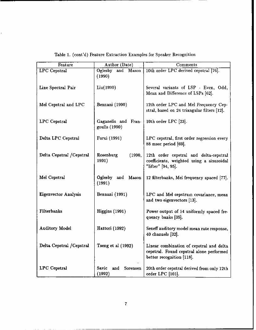
Table 1. (cont'd) Feature Extraction Examples for Speaker Recognition

Feature Author (Date) CommentsLPC Cepstral Oglesby and Mason 10th order LPC derived cepstral [76].

(1990)

Line Spectral Pair Liu(1990) Several variants of LSP - Even, Odd,Mean and Difference of LSPs [62].

Mel Cepstral and LPC Bennani (1990) 12th order LPC and Mel Frequency Cep-stral, based on 24 triangular filters [12].

LPC Cepstral Gaganelis and Fran- 10th order LPC [23].goulis (1990)

Delta LPC Cepstral Furui (1991) LPC cepstral, first order regression every88 msec period [69].

Delta Cepstral /Cepstral Rosenburg (1990, 12th order cepstral and delta-cepstral1991) coefficients, weighted using a sinusoidal

"lifter" [94, 95].

Mel Cepstral Oglesby and Mason 12 filterbanks, Mel frequency spaced [77].(1991)

Eigenvector Analysis Bennani (1991) LPC and Mel cepstrum covariance, meanand two eigenvectors [13].

Filterbanks Higgins (1991) Power output of 14 uniformly spaced fre-quency banks [35].

Auditory Model Hattori (1992) Seneff auditory model mean rate response,40 channels [32].

Delta Cepstral /Cepstral Tseng et al (1992) Linear combination of cepstral and deltacepstral. Found cepstral alone performedbetter recognition [118].

LPC Cepstral Savic and Sorensen 20th order cepstral derived from only 12th(1992) order LPC [101].

7

2.2.1 Linear Prediction Analysis When disregarding the nasal tract and associated

sounds, speech production can be accurately modeled by an all-pole filter excited '-v either a

semi-periodic impulse train or white gaussian noise. This model makes some asbij iptions,

but provides a simplified and fairly accurate model of voiced utterances. Thus, LPC

analysis creates a series of representative coefficients which can subsequently be passed

to a classifier. A good review with mathematical formulations and examples of LPC is

provided by Atal [9] and Makhoul [67]. These features have experienced great use in

vector quantization, discriminant analysis and neural network approaches toward speech

and speaker recognition. However, there is serious limitations in their use in noise, as

Parsons points out,

When the speech signal is corrupted by noise, the assumptions of the all-polemodel are violated and the quality of the estimate suffers. Low signal-to-noiseratios (e.g., below 5 to 10 dB) can cause serious distortion of the model spectraldensity [80:page 165].

2.2.2 Cepstrum Analysis Most recent research has relied extensively on cepstrum

coefficients and cepstrum derivatives. The theory behind this feature space for speaker

recognition is reviewed.

2.2.2.1 Power Cepstrum The cepstrum or power cepstrum is defined as the

power spectrum of the logarithm of the power spectrum of a function [16]. In 1977, Childers

further describes this representation's usefulness.

In practice the power cepstrum is effective if the wavelet and the impulsetrain, whose convolution comprise the composite data, occupy different que-frency ranges.

The authors use the term wavelet to denote some original signal (potentially with echoes

or reverberations) and quefrency is the coinage for the units of the cepstral spectrum.

This description is directly applicable to our model of speech production. We will

usually concern ourselves with short sequences of framed speech data, s(n). This signal

8

can be considered the convolution of an excitation signal, g(n), with a transfer function of

the vocal tract, h(n). At time t,

t

s~,t :gkhn-k (1)k=-oo

Taking the Fourier Transform, the spectrum is as follows.

S(w,t) = 1: s(k, t)e-jwk (2)

The inverse Fourier Transform of the log magnitude spectrum provides,

00

logjS(w,t)I= E ck(t)e-' (3)k=-00

where ck(t) is the kth cepstral coefficient at time t.

It is noted the second transform has been described as both the forward transform

[16, 28, 80] as well as the inverse transform [10, 114], as shown above. However, since

Equation 3 produces a real and even function, the sign of the complex exponential is

irrelevant. By separating the complex exponential into real and imaginary components,

this fact is evident.

loglS(w, t) = • ct(t)cos(wkt)±j 1: ck(t)sin(wkt) (4)k=-c k=-oo

However, the second summation, being an odd function, sums to 0 over these limits.00

log S(w,t)I = ck(t)cos(wkt) (5)A:=-oo

Soong [114] references that a finite order of terms can be used in a Discrete Cosine Trans-

form (DCT) for this representation. He also remarks that since the covariance of these

cepstral coefficients is diagonal dominant, they are very similar to a Karhunen-Lobve (KL)

Transform.

9

Figures 1, 2, and 3 shows the above process on a sample of speech. The samples

correspond to a vowel by a male speaker '. In performing the second transform, in general,

1000

800 VOWEL JY

600

400

200

0

-200

-400

0 100 200 300 400 500 600 700 800 900Samples

Figure 1. Sample Speech (Vowel IY, male speaker)

8000-

4000-

Cr

I I

0 0.5 1 1.5 1.97Time (seconds)

Figure 2. Sample Spectrum. The previous samples correspond to the first voiced region,at approximately 0.2 sec.

the slow moving transfer function is separated from the higher fundamental frequencies of

'It should be pointed out, that based on a sampling rate of 16 KHz, one can easily calculate the pitchof the unknown speaker, as shown in Figure 1. The fundamental frequency (pitch) in this waveform isapproximately 140 - 150 Hz (110 samples).

10

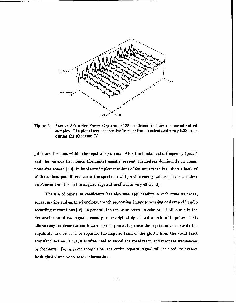
0.351316"; f ( 37

Figure 3. Sample 8th order Power Cepstrum (128 coefficients) of the referenced voicedsamples. The plot shows consecutive 16 msec frames calculated every 5.33 msecduring the phoneme IY.

pitch and formant within the cepstral spectrum. Also, the fundamental frequency (pitch)

and the various harmonics (formants) usually present themselves dominantly in clean,

noise-free speech [80]. In hardware implementations of feature extraction, often a bank of

N linear bandpass filters across the spectrum will provide energy values. These can then

be Fourier transformed to acquire cepstral coefficients very efficiently.

The use of cepstrum coefficients has also seen applicability in such areas as radar,

sonar, marine and earth seismology, speech processing, image processing and even old audio

recording restorations [16]. In general, the cepstrum serves in echo cancellation and in the

deconvolution of two signals, usually some original signal and a train of impulses. This

allows easy implementation toward speech processing since the cepstrum's deconvolution

capability can be used to separate the impulse train of the glottis from the vocal tract

transfer function. Thus, it is often used to model the vocal tract, and resonant frequencies

or formants. For speaker recognition, the entire cepstral signal will be used, to extract

both glottal and vocal tract information.

11

2.2.2.2 Mel-Scale Cepstrum This cepstral representation is considered Mel-

Frequency Cepstral if the spectrum is warped before the second (inverse) Fourier transform.

Additionally, if a filterbank approach is used, these bandpass filters are spaced with appro-

priate bandwidths according to a "mel" non-linearity. Mel or bark scale approximates the

resolution of the human auditory periphery. Mel Frequencies utilize a linear scale up to

about 1 KHz and logarithmic thereafter. Thus, the individual bandwidths of these filters

would increase. The mel-scale can be approximated by,

Mel = (1000/log(2))log(1 + freq/1000)

[80] and is plotted in Figure 4. Another derivation is the bilinear transform. This trans-

3500 ' !

1000/loglO0(2) * loqlO(1+x/0O00) -

3000 - - - - -4--- ---

2 5 0 0 ----- ----. . -- -.. . . . . . .. . . . . .-- --. . . .. - .... ... . . . .. ---- -- --.. ...... . . ............. ...... .... .2500 !

2000

1500 ----- ---- - _ 4 - ------- ---- - -- -

1000

500

0 J ........................ A0 1000 2000 3000 4000 5000 6000 7000 8000

Frequency (Hz)

Figure 4. Mel Frequency Scale [80]

formation is referenced in Kai-Fu Lee [56], crediting Shikano's application of Oppenheim's

transform. Lee describes this transform, an all-pass filter, as follows,

z(z - ,a),(-l<a< 1) (6)

a -aaz-I

a sinww = w+2tan-l( asi ) (7)

1 - acosw

12

where Wew is the converted war, -1 frequencý and positive a lengthens the low frequency

axis. His SPHINX [56] spee h recognition system uses a value of .6 for a, which is compara-

ble to the mel scale. Davis and Mermelstein [19] compared several cepstral representations

for speech recognition and found Mel Cepstrum superior to linear frequency cepstral and

linear prediction cepstral. A recent AFIT thesis by Rathbun [86] examined the Davis and

Mermelstein representations including Mel Frequency cepstral, linear cepstral, linear pre-

dictive cepstral and various first derivatives over time of these features in two dimensions.

These two dimensional representations were used in speech recognition experiments.

2.2.2.3 Complex Cepstrum The complex cepstrum, since is maintains all phase

information, can be used to reconstruct the original signal, often after filtering (liftering) is

performed in the cepstral domain. The complex cepstrum is defined as the inverse Fourier-

transform of the complex logarithm of the Fourier-transform of the original function. The

term "phase unwrapping" is used when performing this analysis. The approach in per-

forming a logarithm on complex data is to separate the complex quantity into a magnitude

and phase component phasor. A two dimensional implementation of this technique was re-

cently documented in AFIT thesis by Lee [57] in performing VLSI image processing. This

representation's usefulness for speech or speaker recognition has not been determined.

2.2.2.4 Linear Predictive Cipstrum In 1974 J.A.S.A. article, B.S. Atal de-

fines the cepstrum as the inverse Fourier transform of the logarithm of the transfer function

[8].

In H(z) = C(z) = ckz-k (8)k=1

Recall that a linear predictive analysis on speech samples attempts to fit the p all-pole

filter defined as,

1 + EP=akz (9)

It can further be shown, based on this all-pole model for H(z), a recursive relation between

the cepstral coefficients Ck and the prediction coefficients ak. By taking the derivative of

A3

(8), the cepstral coefficients can be derived by,

cl = a, (10)k-1

Ck = -(l-l/k)alCk_-, +ak. < k < p (11)l=l

The benefit readily seen through this technique is the reduction in the feature space

dimension. In using FFT or DFTs, the number of coefficients in the output is based on

the order of the FFT , 2 r.* Whereas, in Atal's method, the number would be based on

the number of p poles. Parson's gives a rule-of-thumb for the number of poles p [80].

f= + (12)1000

where f, is the sampling frequency of the original data and y is a "fudge constant" which

is typically 2 or 3 for adding extra poles to the model for flexibility. An example of LPC

cepstral is shown in Figure 5. Note the LPC representation provides the overall shape of

the previous linear cepstral representation.

This feature set is found extensively in the current literature. Most often, the LPC

coefficients are first obtained, then transformed to cepstral coefficients. Atal [10] had com-

pared LPC coefficients, log area ratios, correlation coefficients and LPC cepstral and, for a

limited speaker database, had shown this representation to provide better speaker recog-

nition. Interestingly, Atal found that the Mahalanobis distance measure proved a most

effective distance metric between the LPC cepstral vectors. Soong and Rosenburg [114]

have shown that the higher order coefficients carry as much information as the lower order

coefficients, in achieving speaker identification. Since these coefficients have numerically

smaller values and provide less contribution, it was deemed appropriate to weight them

based on the inverse covariancu of each coefficient. This technique is known as "weighted

cepstral distance." Thus, the Mahalanobis distance measure has proven effective in speaker

recognition experiments.

Atal had also demonstrated that subtracting off the time averages of each coefficient

can remove induced channel characteristics, caused by different recording equipment or

14

-1.223070

19 23

Figure 5. 20th order LPC Cepstral using. Note pertinent spectral shape information ofthe power cepstrum. The plot shows consecutive 16 msec frames calculatedevery 5.33 msec during the phoneme IY.

communications channels. One of the underlying characteristics of cepstrum analysis is

that convolutions in the time domain correspond to additions in the cepstral spectrum,

made possible by the log operation. Thus, transmission induced distortions (convolution

in time) which are approximated as time averages of cepstral coefficients can be removed

via subtraction [8].

2.2.2.5 Cepstral Expansions In signal processing, often the temporal charac-

teristics of the signal contain useful information. This has been shown to be especially

true in speech processing. One simple example is the speech spectrogram, where the hori-

zontal formant track over time depicts various consonant vowel relations. These temporal

characteristics of speech also contains speaker dependent information, for use in speaker

identification. Furui [22] has shown that polynomial expansions of the cepstral time sig-

nals increase speaker identification performance. He examined time average, slope and

curvature of the cepstral coefficients using a 90 msec window (9 - 10 msec frames) using

15

the following transformation.

Poj = 1 (13)

P1j = j-5 (14)

P23 = j 2 -10jj+55/3 (15)

Then, a window of 9 vectors, cj : (j = 1,2,...9), can be represented by three projection

coefficients. The first order polynomial gave the greatest classification improvement.

9

a = (Ec,)/9 (16)j=l

9 9

b = (E-cjPi,)/ E P1, (17)j=1 j=1

9 9

c = (EcP2J)/Z-PE j (18)j=l j=l

Note, the first order can be generalize as a linear regression coefficient over the interval

2K + 1 [56, 114]. This representation is often referred to as delta cepstrum.

K K

rj(t) = ( kc(t+k))/ k2 (19)k=-K k=-K

Soong [114] later demonstrated that transitional patterns contain uncorrelated information

to that of instantaneous cepstral representations, and also showed better resistance to

channel characteristics. Lee, [56] in preliminary tests for the SPHINX system, settled on

only differenced coefficients using a 40 msec window, symmetric with +6 = 20 msec from

the current frame. The mth differenced (or delta) coefficient at time t is simply,

dm(t) = cm(t + 6) - c..(t - 6) (20)

2.3 Classification and Clustering

The end goal for Automatic Speaker Recognition is a reliable decision of an unknown

individual's identity. This section details the numerous ways that classification of a speaker

16

is currently being attempted. Classification is the process of choosing the most probable,

or closest class, by the individual's features from a set of reference features or models. By

grouping a set of related features to a labeled entity, one forms a class. Currently, classifi-

cation can best be divided into pattern matching paradigms, model estimation techniques

(such as Hidden Markov Models), and Artificial Neural Networks (ANN). This represen-

tation is depicted in Figure 6. Gaganelis and Frangoulis state a key introductory point,

Speaker Verification systems rely often on techniques developed for SpeechRecognition. Techniques like Dynamic Time Warping, Vector Quantization,Hidden Markov Modeling, Clustering and Linear Discriminant Analysis arefeatured in many systems [23].

The following sections will present many of these techniques for classification and cluster-

ing; however, it must be pointed out, there exhibits a great deal of overlap between all

these approaches. Table 2 lists the many classification paradigms examined over the past

several years.

2.3.1 Vector Quantization and Distortion Based Classification Though often used

as a communications coding scheme [15], vector quantization (VQ) has proven a computa-

tionally efficient and simple scheme for pattern classification using an appropriate distortion

measure. Vector quantization or clustering analysis determines the optimal representative

k codewords which represent p data points. This procedure creates a codebook, Ak a finite

collection of codewords, which can be used for information coding or classification Clas-

sification is performed by measuring a distortion between the unknown test speaker and

the reference speaker codebooks. The optimal codebook to be created, however, relates

to a particular set of criteria chosen, and in general, will present itself as an optimization

problem with multiple local minima [124].

A recent article critique points out the subtle, yet important similarities between

vector quantization and cluster analysis. Vector quantization, an electrical engineering

concept, attempts to define the best representation or partitioning of data, often used for

communications data reduction or coding. Cluster analysis is a statistical mathematics

discipline which further processes the parametric details of these partitions. This thesis re-

17

Table 2. Classification Techniques for Speaker Recognition

Classifiers Author (Date) Speakers, ID %, CommentsDistortion Atal (1974) 10 speakers, 98% identification, Ma-

halonobis Distance using pooled intraspeaker covariance [8].

DTW Furui (1981) 20, Dynamic Time Warp distortionmeasurement on fixed sentences [221.

K-means, Gaussian Schwartz (1982) Compared Gaussian classifiers to K-Estimation means and Mahalonobis Distance,

non-parametric outperformed [105].

HMM Poritz (1982) Application of 5 state ergodic HMMto speaker verification [83].

VQ Soong (1985) First Speaker dependent codebooks,voiced and unvoiced speech [113].

VQ Soong (1988) 2 Codebooks, 1 instantaneous and 1temporal [114].

MLP Oglesby and Mason (1990) 10, 92%, Backprop learning, singlelayer with 16 - 128 hidden nodes,Equal recognition to VQ s5.1.10.

K-means/ LVQ Bennani et al (1990) 10, 95 - 97% [12].

HMM Rosenburg et al (1990) 20, 98.8 - 99.1%, Used k-means to seg-ment the utterance into acoustic seg-ment units, also examined phoneti-cally labeled speech [94].

HMM Savic and Gupta (1990) 43, 97.8%, 5 HMM models represent-ing broad classes [102].

GMM Rose and Reynolds (1990) 12, 89%, Only 1 sec of test speech [93].

18

Table 2. (cont'd) Classification Techniques for Speaker Recognition

Classifiers Author (Date) Speakers, ID %, CommentsBinary Partition Rudasi and Zahorian (1991) 47, 100%, TIMIT corpus, need N(N-

1)/2 binary MLP classifiers.RBF NN Oglesby and Mason (1991) 40 , 89% true talker, different manner-

isms of speech.GMM Rose et al (1991,1992) 10, 77.8%, Integrated noise model into

GMM, GMM on Original clean speech- 99.5%.

Discriminator Higgins and Bahler (1991) 24, 80% true talker, KING cor-Counting pus, multivariate gaussian, count

wins/speaker summed over frames.VQ Matsui and Furui (1991) 9, 98.5 - 99.0 %, Voice/Unvoiced or

2-state HMM, New Distortion mea-sure (DIM), Talker variability normal-ization (TVN) individually weightsfeatures.

HMM Rosenburg (1991) 20, 96.5 - 99.7%, Whole word L-to-RHMM, text dependent (digits), com-pared to VQ.

Time Delay NN Bennani and Gallinari (1991) 20, 98%, First a Male / FemaleTDNN, then a 10 output (speak-ers) TDNN using 2 hidden layers(hierarchical).

HMM, VQ, ANN Hattori (1992) 24, 100 %, TIMIT corpus (fe-males), Predictive NN (recurrent)within HMM, compared to VQ and

MLP classifiers.CPAM (GMM) Tseng et al (1992) 20, 98.3% identification, CPAM - Con-

tinuous Probability Acoustic Map,mixtures of Gaussian kernels with andwithout HMM.

MLP Gong and Haton (1992) 72, 89 - 100%, Trained MLP to in-terpolate between speaker utterances(phoneme), needs labeled speech(vowels).

VQ Kao et al (1992) 26 (51), 93.3% (67.6), KING corpus,11 broad class codebooks of 10 vec-tors, Needs labeled speech.

19

4,PRE-P -ROCESSIN ]

SAMPLED DATA

PATTERN MATCHING MODEL ESTIMATION ARTIFICAL NEURALNETWORKS

- DTW - GAUSSIAN MIXTURE MODEL - TRAIN ANN

-CLUSTERING (VQ) - HIDDEN MARKOV MODEL

0 Ci

0 000P,0 0 0 0d••(X, Ci) S1 S2 S3 0

MINIMUM "DISTORTION" MAXIMUM LIKELIHOOD LEARN DISCRIMINANT

FUNCTION

NON-PARAMETRIC PDF PARAMETRIC PDF OUTPUTS ESTIMATEESTIMATION ESTIMATION CLASS PROBABILITY

Figure 6. Speaker Recognition Classification Paradigms.

20

gards all techniques from both disciplines as (iterative) means to the optimal representation

of the underlying probability density function of some unknown random process.

2.3.1.1 Objective Function and Necessary Criteria The objective of this quan-

tization design procedure solves for the global minima of some objective function, typically

least mean squared error. Bezdek [14] defines this distortion function as,

p k

JI(U, Y; X) = E uij(llxi - yi 11), (21)s=l j

where, X and Y are the set of training data {x 1,...,xp} and codewords {Y.,'",yk}

respectively, U contains the membership values of each xi to the codeword yj, and •J

is typically the Euclidean norm on the X space. A vector quantizer is said to be optimal

if no other quantizer has a smaller overall distortion. The two necessary conditions for

optimality [1261 are

1. Nearest neighbor: A training vector is mapped to the "nearest" codebook vector,

based on a particular distortion metric. If the codebook contains k vectors, this

mapping results in a partitioning of the input space into k regions [126, 51, 53].

2. Centroid. The codevector for a given partition is the mean or expected value of the

partitions' elements.

For LBG and k-means [117], the memberships uij are defined by nearest neighbor and take

on values of 0 or 1. By extending this membership to the continuous interval (0, 1], fuzzy

set theory is applied to clustering [14, 41, 108].

2.3.1.2 Modeling the Density Function Vector quantization produces an ap-

proximation to the continuous pdf, p(x), of a variable x in R" using a finite number of k

codewords [51, 53]. Optimality of this approximation refers to minimizing an error function

such as,

E Jlx - mcJJrp(x)dV, (22)

where m, is the "best-matching" codeword and dV, is an incremental volume in the Rn

space. As previously stated, there are no closed form expressions for the placement of the

21

k codewords, and iterative or learning schemes are used. If p(x) were known, numerical

and statistical techniques could directly determine centroids, number of classes and class

boundaries [21, 53]. Kohonen references the fact that the point density function of the k

vectors approximates the true pdf as the ratio of data dimensionality over distortion metric

increases.

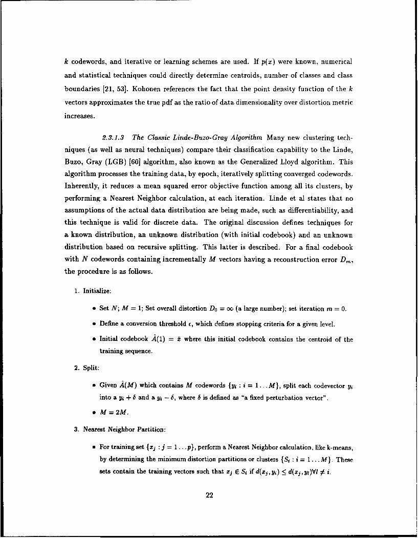
2.3.1.3 The Classic Linde-Buzo-Gray Algorithm Many new clustering tech-

niques (as well as neural techniques) compare their classification capability to the Linde,

Buzo, Gray (LGB) [60] algorithm, also known as the Generalized Lloyd algorithm. This

algorithm processes the training data, by epoch, iteratively splitting converged codewords.

Inherently, it reduces a mean squared error objective function among all its clusters, by

performing a Nearest Neighbor calculation, at each iteration. Linde et al states that no

assumptions of the actual data distribution are being made, such as differentiability, and

this technique is valid for discrete data. The original discussion defines techniques for

a known distribution, an unknown distribution (with initial codebook) and an unknown

distribution based on recursive splitting. This latter is described. For a final codebook

with N codewords containing incrementally M vectors having a reconstruction error D,,

the procedure is as follows.

1. Initialize:

"* Set N; M = 1; Set overall distortion Do = o0 (a large number); set iteration m = 0.

"* Define a conversion threshold c, which defines stopping criteria for a given level.

"* Initial codebook A(1) = 2 where this initial codebook contains the centroid of the

training sequence.

2. Split:

"* Given A(M) which contains M codewords {yi : i = 1 ... M}, split each codevector yi

into a yi + 6 and a yi - 6, where 6 is defined as "a fixed perturbation vector".

"* M=2M.

3. Nearest Neighbor Partition:

e For training set {zj : j = 1 ... p}, perform a Nearest Neighbor calculation, like k-means,

by determining the minimum distortion partitions or clusters {Si : i = 1 ... M}. These

sets contain the training vectors such that zj E Si if d(zj, y,) <_ d(xj, yi)Vl 6 i.

22

* Calculate distortion over entire training set.

P

D Tmin d(xi,y). (23)Pj=1yEAn(M)

4. Check Convergence:

"* If (Din- 1 - Dm)/Dm <_ c, stop with Am(M) being the final converged reproduction

codebook for the current level. Else, m = m + 1, Go to Recompute Centroids.

"* If M = N Stop. Else, Go to Split.

5. Recompute Centroids: Recalculate the centroids as the mean of the current partitions, Si.

The authors [60] write this as,"Find the optimal reproduction alphabet."

Yi = 1 E z. (24)z. I"ES,

More recently, competitive learning approaches have been developed which allow

a codebook to learn on-line, as training data is presented [53]. Such examples include

adaptive k-means, competitive learning schemes, and specifically the self-organizing feature

maps by Kohonen [44, 49, 50, 51].

2.3.1.4 Generalized Competitive Learning Competitive learning systems are

usually feedforward multilayer neural networks [53]. These networks adaptively quantize

the pattern space spanned by some random pattern vector x [53]. In competitive learning,

a series of processing elements or nodes each defined by their weight (synaptic) vectors

compete to become the "winner", and subsequently become updated. A node wins the

competition for an input x if its synaptic vector m, is closest to x, usually in Euclidean

distance, than all other vectors. This closest vector gets modified in the direction toward

the input x, by some scaled amount. Each synaptic vector mr represents local regions

about mj [53].

In order to create Kohonen's spatial ordering of the nodes, a neighborhood concept

was developed, such that a winning node and the surrounding neighbors on a lattice are

updated toward the training point. This neighborhood concept also complicates the proof

23

of convergence for SOFMs, except in the simplest of cases. However, it is also thought

that this capability may aid in the convergence to non-local minima [126].

2.3.1.5 Kohonen Learning Rule A Kohonen lattice for a two dimensional out-

put space is shown in Figure 7. Typically a two dimension output map is used, yet other

output mappings may prove more desirable [50]. In fact, the choice of output dimension can

be based on quantitatively defining neighborhood preservation [11]. Each node is assigned

a reference vector mn and the input vector x is presented to all nodes. The best-matching

unit or winner c at iteration t is determined by,

IIx(t) - m6(t)ll = mnm jx(t) - m1(t)JI (25)

The learning rule proceeds as follows,

mi(t + 1) = mi(t) + a(t)[x(t) - ma(t)] V i E N,(t)

mi(t + 1) = m,(t) V i V N,(t). (26)

Here Ne(t) is the neighborhood size around the winning node c at iteration t, with a(t)

determining the learning rate at time t. Kohonen often describes these as linear mono-

tonically decreasing functions. Interestingly, the neighborhood function could exist as a

continuous function of relative lattice distances. A typical choice could be gaussian [11].

Since learning is a stochastic process, where the vectors x are random vectors, the algo-

rithm should iterate through a very large number of steps, on the order of 100,000 [50]. A

hueristic for iterations is more than 500 times the number of nodes [50, 91]. Ranges for

a have been given as beginning near unity and dropping to .1 in the first 1000 iterations,

followed by many iterations (10,000) with a below .01 [50].

The update rules can be chosen from a linear schedule, a hyperbolic schedule or

exponentially [124]. However, many parameters must be chosen, often adhoc, such as

update schedule, total iterations, occurrence of resets and the decision to implement a

conscience [91, 126]. A supervised modification to Kohonen's learning algorithm results in

the Learning Vector Quantization algorithm (LVQ). LVQ requires an initial guess at the

24

Nc(t)

Mi

Mi

X1, X2, X3 ... XN

Figure 7. Kohonen 2D Lattice. This representation of the output space map shows then-dimensional input training vector x, two node locations (weights) mi and inj,

with some winning node, labeled c (center). At some iteration time t, thereexists some neighborhood about the winner, N,(t).

25

codebook, and then attempts to more efficiently define the boundaries between classes,

using a supervised scheme with labeled data. Kohonen, himself, suggests first using a

Kohonen feature map to create a broad distribution of codevectors, then use LVQ to "fine

tune" the map [51].

The learning vector quantizers (LVQ) should be used if "the self-organizing feature

map is to be used as a pattern classifier [52]." Kohonen further expands the goals of LVQ in

that, for classification, only decisions made as class borders count. LVQ attempts to create

"near-optimal" class borders in terms of Bayes decision theory. Kohonen points out [75]

that only LVQ1 and LVQ3 are self-stabilizing with continued learning; LVQ2 optimizes only

relative distances of codebooks vectors around class borders, and may not truly define the

actual class boundaries. Another important aspect of LVQ is that the vector quantization

does not reflect the underlying density functions.

2.3.1.6 Conscience Let the input space be divided into k decision classes or

partitions D, ... Dk. Each has an associated class probability p(Di) which integrates the

unknown probability density p(x) over the local region Di [53). Then if all p(Dj) = i/k, a

uniform partition exists. DeSieno [20] developed a modification to the "Kohonen learning"

rule to specifically perform a better approximation to the underlying probability density

function by insuring uniform partitions were created. This work was motivated by earlier

Rumelhart and Zipser (1985) research indicating that it was possible for nodes to never

win, when using a competitive learning rule. However, both the earlier research and De-

Sieno's experiments used a null neighborhood, including only the winner. This could be

considered general competitive learning and not Kohonen learning, where spatial order-

ing and topology preserving characteristics are inherent. Kohonen noted that a valuable

characteristic for a trained SOFM was to have each node win the competition with equal

probability. DeSieno added a bias term to the Kohonen competition equation, Equation

25, based on the frequency of winning. Let pi represent the win rate for node i, defined

as number of wins (hits) divided by number of iterations (presentations) of data, h/t. De-

Sieno presented an iterative calculation of this rate which also is impartial to "fluxuations

26

in the data." Let y, be the "activation" for the nodes where

y, = 1, if IIX - mi12 < JIx -m _ i"12 V j / i

yi = 0. otherwise. (27)

The win rate is then

pi(t + 1) = pi(t) + B[y, - pi(t)] (28)

where 0 < B < 1. If one substitutes simply h/t in the above equation for pi. B should

monotonically decay as 1/(t + 1). Desieno uses a value of B = .0001. The competition

process now introduces a bias term bi in determining a winner c,

IIx(t) - mc(t)II - b = -min IIx(t) - m,(t)JI - b, (29)

where this difference of fairness term bi is,

b, = C(llk - p,). (30)

The constant C represents the bias factor and determines the distance a losing node can

achieve before entering the solution [20]. DeSieno used a C = 2.5; this thesis typically

relates this value to the spread of the data, such as using the standard deviation of the

training set [96].

Rogers and Kabrisky [911 discuss a modification without incorporating this bias term.

Nodes are removed from competition when their win rate is greater than a threshold,

inversely proportional to number of nodes, k. Thus, nodes must satisfy

pi 0 I (31)

to compete, where t is the current iteration and /3 is the conscience factor 1 S 03. The

larger values of P3 results in less conscience; nodes "don't feel guilty about" winning much

more than others. As an example, a #3 of 1.5 is considered a lot of conscience; whereas a

value 5 is very little.

27

2.3.1.7 Statisticat Clustering Analysis The discipline of statistical pattern

analysis provides both parametric and non-parametric means of determining an unknown

function probability density. Inherently, the two approaches discussed (LBG and Kohonen)

attempted to obtain the optimal solution to the LMS objective function. Many of the con-

cepts presented in this section are parametric approximations or kernel generalizations of

these previous approaches. All the probability theory specifically applied to non-supervised

clustering is provided in the book Pattern Recognition: A Statistical Approach [21] and can

also be found in Tou and Gonzalez [117].

The basic statistical re':ognition problem is to decompose a mixture probability den-

s~ty function (pdf), p(x), into an appropriate number c of class conditional pdfs.

p(x) = ZPip(x w,) (32)i=i

Devijver and Kittler [21] point out,

When the class-conditional distributions are parametric of a known form,the unknown parameters of the distributions can be estimated from the databy well-known mixture decomposition techniques [21:pg 383].

The usually assumed parametric distribution is the multivariate gaussian. These authors

describe various analytical approaches toward acquiring these class probabilities. However,

the assumptions are based on marginal pdfs, where unimodal analysis can be performed.

This is referred as mode separation. Though not always valid, the authors point out using a

Karhunen-Loeve (KL) expansion before this mode separation can be used. The possibility

,xists that multiple modes may still overlap in the transformed KL eigenvector axes.

A statistical alternative to the direct parametric approach is clustering the data into

homogeneous partitions, based on "similarities." The similarities are based on distance or

distortion measures. When comparing clustering to the above parametric procedure, often

data found in the same cluster would be associated within the same gaussian mode with

the overall pdf, p(x), Equation 32. Statistical clustering procedures include dynamical

(iterative) approaches and hierarchical algorithms.

28

The k-means algorithm performs a nearest neighbor calculation using k arbitrary

clusters, and calculates the centroids (means) of these partitions. The algorithm terminates

whenever the algorithm converges. However, this representation of cluster mean can be

extended to generalize more sophisticated models. Let a cluster 17j be represented by some

kernel Kj, defined by a set of parameters Vj. Next, let (y, Kj) be a measure of similarity

(distance metric) between a vector y and the cluster represented by Kj. Natural choices for

K include normal distributions defined by mean and covariance as well as Karhunen-Loeve

expansions of the original cluster patterns. On the other hand, the hierarchical approach

begins with all data points as clusters and merges similar ones iteratively.

The authors [21] emphasize that non-supervised classification methods should be ap-

plied with great care. Such "practical problems ... as scaling of the axes, metric used,

similarity measure, clustering criteria, number of points in the analyzed set, etc." will all

greatly affect the results of the analysis. Other insights include these dynamic clustering

methods usually being "computationally very efficient", yet the "chosen model rarely re-

flects the true probabilistic structure of the data. In such situations, the dynamic clustering

algorithm can give rise to an unrealistic grouping of data."

2.3.1.8 Distortion Metrics A number of distortion metrics have been devel-

oped both in the mathematics community [14][21:pg 232][80:Chapter 7] and specifically

for speech processing [29]. These include Minkowski, Euclidean, Chebychev, Quadratic

and nonlinear, as well as Itakura-Saito Distortion and Itakura Prediction residual. This

thesis will examine those types meaningful for speech (cepstral) representations, such as

Euclidean distance and more specifically, squared distance,

d(x, in,) " (x - m,)T(x - in,) (33)

and also the Quadratic,

d(x, m,) = (x - mn)TR(x - m,) (34)

where R is a positive definite scaling matrix. Typically this can be the full covariance of

the data set, or anproximated by the diagonal elements if diagonal dominant. Also, R

29

may be a weight such as the squared index, i2. This is known as root power sum (RPS)

distortion. However, an outstanding issue will be the appropriate distortion metric for

auditory features. If the assumption can be made that the human auditory periphery is

merely doing a spectral analysis, then appropriate distortions can be chosen.

Another related concept is the probabilistic distance. For statistical pattern recog-

nition (and for any recognition problem), the analysis of feature choice is important. A

measure of class separability based on the complete probabilistic structure of the classes

can be related as a "distance" between class pdfs. Similarly, the concept of probabilistic

dependence can be examined. Several measures exist for determining separability of fea-

tures based on class densities. Such measures include Chernoff, Bhattacharyya, Matusita,

The Divergence, Patrick-Fisher and Lissack-Fu [21:pg 257-258]. However, this analysis cur-

rently cannot be extended beyond two class problems. Due to the numerical calculations

and required estimates of the probability density functions, other simpler criteria exist

where non-parametric density functions exist. These probabilistic separability measures

(still only useful for two class problems) are efficient for parametric pdfs, and consideration

can be made on parametric approximation of unknown non-parametric pdfs. For example,

a gaussian mixture model may be fit to a data set.

2.3.1.9 Other Quantizer Designs Simulated annealing (SA) techniques and

several variations have demonstrated experimental results superior to LBG [124, 1271.

Simulated annealing is the process that relates optimization strategies to the annealing

or cooling of molten metal. The solutions for this problem can be extended to any op-

timization problem, which attempts to minimize some objective function. Zeger et al

[126, 127] compare the analysis of simulated annealing to that of LBG and Kohonen

learning paradigms. These authors extended the Kohonen neighborhood concept using

a "soft-competition" algorithm.

For the past several years, vector quantization techniques have demonstrated high

recognition accuracies. Currently, Hidden Markov Model techniques are being researched

extensively and compared to VQ results. Some studies have shown 50% improvements

30

over Dynamic Time Warping and comparable results to Vector Quantization using both

discrete HMMs [951 and continuous ergodic HMMs [681.

2.3.2 Hidden Markov Models! Gaussian Models Hidden Markov models are exten-

sively being documented in the current literature. Whereas pattern matching techniques,

like DTW and Vector Quantization, create templates which represent the training data, an

HMM creates a model of the training data. These models are characterized by a Markov

process of state transition probabilities, in addition to a stochastic process of output proba-

bilities. Initially, ergodic HMMs were researched, yet left-to-right models have been shown

to be applicable and successful to speech processing. Lastly, Hidden Markov models can

be implemented with either a discrete or a continuous output probability density function

(pdf). In the former case, a vector quantization approach is often used to create a finite

representation alphabet for each state, with associated probability distribution for each

codeword. In the continuous approach, a probability density function, like a gaussian, is

used for the output pdf for each Markov state. A good review on Hidden Markov Models is

provided in Rabiner [84] and Rabiner and Juang [851. This section will summarize recent

HMM initiatives and recognition accuracies.

Only a few experiments have been reported on speaker recognition using a Hidden

Markov Model. Poritz provided the initial work for speaker verification using a 5 state

ergodic HMM [83]. Interestingly, it turned out that the 5 states naturally represented 5

broad classes of speech: voicing, silence, nasals, stops, and frication. His results showed

100% recognition for a small 10 speaker database using text-dependent training.

Rosenburg, Lee, Soong et al [95] examines talker verification using a whole word

HMM. Their vocabulary consists of continuous digits for a 20 speaker corpus, speaking with

error rates of 3.5% and .3% given for 1.1 and 4.4 seconds of test speech respectively. In this

paper, the authors propose that the successes of speaker-independent word and subword

HMMs for speech recognition can be applied to speaker-dependent talker verification tasks.

The models use a 10 state continuous left-to-right HMM with a Gaussian mixture defining

the output pdf. The mixtures contain M components (ranging from 1 to 9) which are

estimated by clustering the utterance into various segments or states and clustering the

31

training data into M clusters. A Viterbi algorithm derivative, referred to as the Viterbi

frame-synchronous search, is used to provide maximum likelihood scores. DTW word

templates are compared with a final score created by a concatenation of individual DTW

word scores. Comparisons to DTW indicate 50% improvemeii by this technique.

Rosenburg, Lee and Soong's earlier work [94] provides the results of an HMM ap-

proach to talker verification using two different types of sub-word HMM data, phone-like

units (PLUs) and acoustic segment units (ASUs). The database used only 20 speakers

speaking only isolated digits. The authors point out that these results can only be sugges-

tive toward text independent large vocabulary databases. The models used a 2 and 3 state

continuous left-to-right HMM with a Gaussian mixture defining the output pdf. The mix-

tures contain M components which are estimated by clustering the utterance into various

L segments and clustering the training data into M clusters. Their results are in terms of

equal error rate 2 which is based on the test speaker probability against all others in the

database, as a function of test time. Comparisons to earlier work by Tishby indicate that

the left-to-right ASU segmentation may be superior to an ergodic model. The explanation

offered is due to the greater temporal detail in a concatenation of left-to-right models.

Vector Quantization perform only a few percent less, which is attributed to the lack of any

temporal information in the clustering process. Overall, equal error rates are 7-8% for a .5

sec test utterance, and less that 1 % for a 3.5 sec utterance, with improvements possible

by updating the models with test data.

Savic and Gupta [102] classify the speech signal based on vowels, fricatives, plosives

and nasals. This approach better represents the model of the vocal tract which changes

during production of these four "broad phonetic categories." A five state HMM is tested,

with a Viterbi algorithm obtaining the maximum likelihood that the frame is assigned to

a state (class). Their conclusions are noteworthy,

...the conclusion can be drawn that better performance can be achieved by rep-resenting each phonetic category by a different model, and by making the final

2Parsons [80] uses "equal error rate" between false rejections and false acceptance, usually plottedagainst some threshold.

32

verification decision based on a weighted combination of scores for individualcategories. Also, our results show that plosives do not have much speaker dis-crimination capability and hence, all classes of phonemes must not be used tomake the verification decision.

Recognition errors rates of 2.32% for 43 speakers are shown. These results reflect those of

a much earlier study by Poritz [83].

Most recently, Matsui and Furui [68] have provided a detailed comparison of Vector

Quantization recognition performance to both discrete and continuous HMMs for both

speaker identification and verification. A database of 46 speakers speaking at different

rates (normal, fast and slow) was used. Identification results for the continuous HMM and

VQ were comparable, about 90% to 95%. Discrete HMM performed at accuracies 5% to

18% below this. For the verification task, the VQ and continuous HMMs again were as

robust at approximately 97% to 98%.

Some researchers are manipulating the Markov model itself, to increase recognition

performance. Often these changes violate the Markov properties and are thus labeled

Hidden Semi-Markov Models (HSMM) [36, 99]. One such change often performed is the

explicit modeling of state durations separately. Huang combines both Discrete and Con-

tinuous HMMs, labeled Semi-Continuous Hidden Markov Models (SCHMMs) [36]. The

author claims that this technique provides a good solution to the fine detail of continuous

HMMs and insufficient training data to provide a good discrete HMM. Since a Markov

process determines state transitions, conventional HMMs are weak in modeling state du-

rations, especially for speech. This new SCHMM method, not only models the state tran-

sition and output probabilities, but also models the state duration probabilities explicitly.

The definition is follows: "The probability of state duration ... di(r) is the probability of

taking the self-loop at state i for r times." These parameters can be estimated from the

observations, along with the other HMM parameters. Thus, the transition from state i

to state j must include not just the state transition probability, but also all the possible

time durations that may occur while in state i. Gu et al [30] demonstrated 1.9% to 9.0%

improved recognition rates in using a bounded state duration HMM. These bounded states

33

force a minimum and maximum duration value for each state. The authors also compare

this approach to Poisson and gamma state distributions.

Another type of speaker model demonstrated in the literature uses gaussian mixtures.

An article by Rose and Reynolds [92] specifically address speaker identification in noisy

environments. The authors present two approaches. First, the background noise is inte-

grated into the voice model. Thus, a noise process is added to the Gaussian Mixture Model

with a maximum likelihood calculation being performed on this aggregate model. Both an

additive and maximum noise model is examined. The second approach preprocesses the

speech before the classification steps. This technique is based on spectral subtraction using

long-term averages of filter bank energies. Database consists of conversational speech from

10 speakers over long distance channels. The author's choose a 32 probabilistic Gaussian

mixture density, which have a diagonal covariance matrix. Error rate range from 38.0%

to 19.4% identification, compared to the original 99.5% rate for clean speech. Clearly this

shows the limitations of current methods on noisy telephone quality speaker identification.

A more recent article by the authors [88] examines the modeling of both the background

noise environment and the speakers separately with GMMs. In this innovative process,

the likelihood of the observation sequence combines the two independent GMM models for

each speaker.

2.3.3 Artificial Neural Network Classification The following methods can be con-

sidered Artificial Neural Network schemes, in that many incorporate a simplified processing

element, which could be exaggerated as a real neuron. This section details current examples

found in the literature on Multi Layer Perceptrons, Time Delay Neural Networks, Radial

Basis Functions and other supervised learning approaches to the classification problem of

speaker recognition.

Bennani [13] demonstrates a Time-Delay Neural Network (TDNN) for feature ex-

traction and classification. The DARPA TIMIT database was tested and an average iden-

tification rate of 98% is given for 20 speakers. Preprocessing is done by 16th order LPC

coefficients as the parameter space on windows of 25.6 msec. Then, each sentence is further

divided into windows of 25 consecutive frames (approximately .6 sec), with this particular

34

choice based on earlier research by Atal [10]. Speaker identity is decided though a two layer

classifier. First, a Male-Female classification is accomplished. The article states, "Moti-

vations for this modular architecture are multifold. First it has long been observed that

speech spectra tend to form two clusters according to the sex of the speaker." A second

recognizer chooses speakers.

A binary partioned Neural Network was recently demonstrated to be a successful

strategy for ASR [98]. Each network is trained for a single person; however, it requires

N * (N - 1)/2 classifiers for N reference speakers. The DARPA TIMIT database is used

with 47 talkers from a single dialect (there are 8 American English dialects recorded on

TIMIT). The LPC Cepstral coefficients were used as features (order 15). Error rates

published are 0% for 47 speakers reached within eight seconds of test data. The article is

quick to point out the limitations of this technique.

(These will) classify with 100% accuracy as long as each of the BinaryClassifiers performs correctly. The performance of [these] approaches, however,may degrade differently if not all the binary classifiers work perfectly.

Oglesby and Mason [77] research a Radial Basis Function Network as a classifier. A

40 speaker corpus, using only the digit set is tested. Noteworthy is that their database

contains each speaker recorded in five different mannerisms: loud, soft, questioning, angry

and normal. The feature space is the first 10 cepstral coefficients acquired through a

12 critical band filterbank of mel-frequency spaced filters. Results are compared to VQ

using codebook sizes of 32, 64 and 128 as well as Multi Layer Perceptrons (MLP) with

32, 64 and 128 hidden nodes. Better performance is shown for Radial Basis Functions

with performances of 8%, 20% and 22% for normal, angry and soft speech respectively,

outperforming both VQ and MLP techniques. These unique results show the greatly

varying effects of intra speaker variability, which is often neglected in the literature.

The two authors earlier [76] vary the hidden layers and number of nodes in a feedfor-

ward Artificial Neural Network. The "personalized" NN is trained active for an individual's

speech including signals from other speakers. The intent of this approach is for the NN

to "learn" unique characteristics of the individual. Their database contains utterances of

35

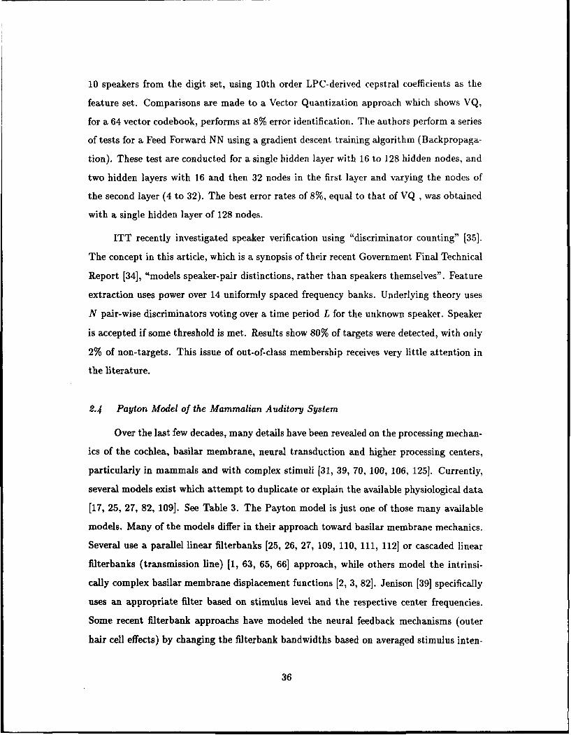
10 speakers from the digit set, using 10th order LPC-derived cepstral coefficients as the

feature set. Comparisons are made to a Vector Quantization approach which shows VQ,

for a 64 vector codebook, performs at 8% error identification. The authors perform a series

of tests for a Feed Forward NN using a gradient descent training algorithm (Backpropaga-

tion). These test are conducted for a single hidden layer with 16 to 128 hidden nodes, and

two hidden layers with 16 and then 32 nodes in the first layer and varying the nodes of

the second layer (4 to 32). The best error rates of 8%, equal to that of VQ , was obtained

with a single hidden layer of 128 nodes.

ITT recently investigated speaker verification using "discriminator counting" [35].

The concept in this article, which is a synopsis of their recent Government Final Technical

Report [34], "models speaker-pair distinctions, rather than speakers themselves". Feature

extraction uses power over 14 uniformly spaced frequency banks. Underlying theory uses

N pair-wise discriminators voting over a time period L for the unknown speaker. Speaker

is accepted if some threshold is met. Results show 80% of targets were detected, with only

2% of non-targets. This issue of out-of-class membership receives very little attention in

the literature.

2.4 Payton Model of the Mammalian Auditory System

Over the last few decades, many details have been revealed on the processing mechan-

ics of the cochlea, basilar membrane, neural transduction and higher processing centers,

particularly in mammals and with complex stimuli [31, 39, 70, 100, 106, 125]. Currently,

several models exist which attempt to duplicate or explain the available physiological data

[17, 25, 27, 82, 1091. See Table 3. The Payton model is just one of those many available

models. Many of the models differ in their approach toward basilar membrane mechanics.

Several use a parallel linear filterbanks [25, 26, 27, 109, 110, 111, 112] or cascaded linear

filterbanks (transmission line) [1, 63, 65, 66] approach, while others model the intrinsi-

cally complex basilar membrane displacement functions [2, 3, 82]. Jenison [39] specifically

uses an appropriate filter based on stimulus level and the respective center frequencies.

Some recent ifiterbank approachs have modeled the neural feedback mechanisms (outer

hair cell effects) by changing the filterbank bandwidths based on averaged stimulus inten-

36

Table 3. Several Auditory Models and their Features

Author (Date) Channels, Frequency Range, Characteristics

Ahn (1990) 20, 200 Hz - 3500 Hz, Filterbank developed by ArmstrongLab, combined with Seneff Inner Hair Cell/Synapse andGSD, modified filterbank GSD [1].

Ghitza (1986, 1987) 85, 200 Hz - 3200 Hz, Filterbanks, Ensemble Interval His-togram (EIH) analyzes threshold crossings of parallel filter-bank outputs. Measure of temporal characteristics, noiseevaluation. [25, 26].

Ghitza (1988) Added feedback to EIH.

Jenison (1991) Iso-intensity maps, create a suite of filters for each channelbased on intensity of signal [39, 40].

Lyon (1986) 49, -,Multi Channel AGC, to change the filter tuning charac-teristics [65]

Lyon/ Mead (1988) 430, -, CMOS implementation with AGC [66].

Payton (1986, 1988) 20, 400 Hz - 6600 Hz, Composite model, BM displacement ofSondhi and Allen, IHC of Brachman [82, 81]

Seneff (1984) 32, 200 Hz - 2700 Hz, Generalized Synchrony Detection(GSD), a measure of the temporal synchrony to each CF[110, 109].

Seneff (1986, 1988) 40, 130 Hz - 6400 Hz [111, 1121.

Others and Applications Cohen [17], Kates [47, 48], Hunt [37, 38], Liu [64, 63], Pat-terson [6], Meddis[6], Shamma [6].

37

sity [27, 39, 63, 65, 66]. This allows the filtered responses to better match physiological

data, by increasing the coverage under the response profiles of the filterbanks. Recent au-

ditory models also attempt to provide both spectral and temporal synchrony information.

Next, the Payton model, as well as other model comparisons, will be analyzed in as a

preprocessor for feature extraction.

Payton chose to combine the best representations which were based on physiological

measurements and contained the least simplifying assumptions. The overall model is pre-

sented in Figure 8. The model has been coded in 'C' [90] and logically separated into three

stages. It should be pointed out that the model, in all three main stages, is required to solve

simultaneous differential equations. The method used is based on the central difference

approximation [3]. This technique replaces derivatives with difference equations. For ex-

ample, the function C(t) and its first and second derivatives can be discretely approximated

as follows, where T is the sampling period between discrete approximations.

C(t) = C(n) (35)

a(1.t = (C(n) - ((n - 1))/T (36)

a2(1at2 = (C(n + 1) - 2((n) + ((n - 1))/T 2 (37)

In Allen and Sondhi's axticle [3], the authors note this technique provides stable equations

if 1/T is greater than 7r times the highest resonant frequency. The current model uses a

sampling frequency of 160 KHz.

2.4.1 Stage 1/ Middle Ear The first stage models the middle ear filtering. As

mentioned, this resembles a low pass filter. The input to this stage is sampled data,

representing sound pressure at the eardrum. Based on Guinean and Peake (1967), a ratio

of stapes velocity to tympanic membrane pressure can be solved through circuit analysis.

Figure 9 shows an example of a TIMIT Database utterance, with the transformation to

stapes velocity given in Figure 10.

2.4.2 Stage 2/ Basilar Membrane The second stage of the Payton model performs

the basilar membrane mechanics. Using the developments of Allen and Sondhi [2], dis-

38

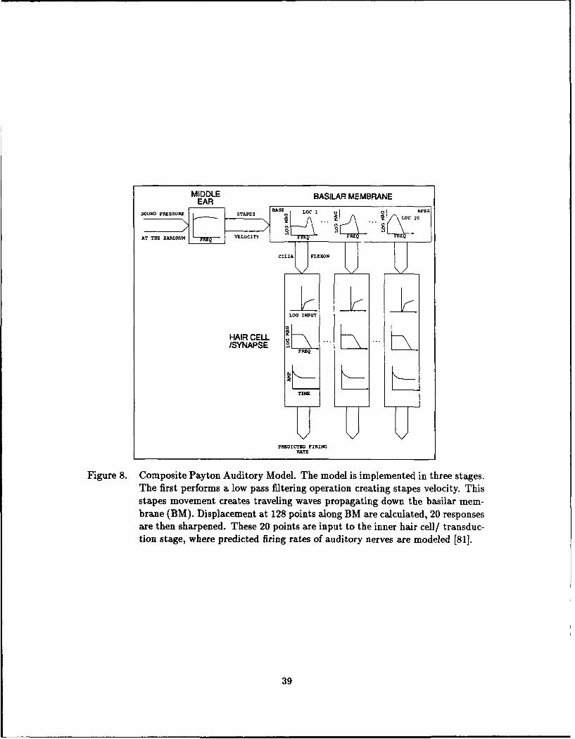
MIDDLE BASILAR MEMBRANEEAR

SOUND PRESSURE SAE AE O

LOG INPUT

HAIR CELL/SYNAPSE L ...

FREQ

TIME

PREDICTED FIRING

RATE

Figure 8. Composite Payton Auditory Model. The model is implemented in three stages.The first performs a low pass filtering operation creating stapes velocity. Thisstapes movement creates traveling waves propagating down the basilar mem-brane (BM). Displacement at 128 points along BM are calculated, 20 responsesare then sharpened. These 20 points are input to the inner hair cell/ transduc-tion stage, where predicted firing rates of auditory nerves are modeled [81].

39

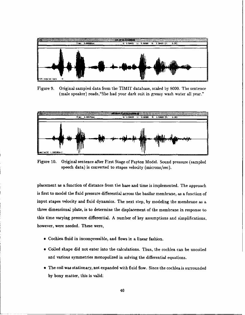
Tfie O.0]0IOsec : 0: 3.59400 L: U ].O000 • R: 3.58400 (F: 0.28)

$D.-.94 "at3.0 -9

Figure 9. Original sampled data from the TIMIT database, scaled by 8000. The sentence(male speaker) reads,"She had your dark suit in greasy wash water all year."

Time: O. 9?Ssec 0: 3.58400 L: 0.000 R: 3.59400 (F: 0.28)

Figure 10. Original sentence after First Stage of Payton Model. Sound pressure (sampledspeech data) is converted to stapes velocity (microns/sec).

placement as a function of distance from the base and time is implemented. The approach

is first to model the fluid pressure differential across the basilar membrane, as a function of

input stapes velocity and fluid dynamics. The next step, by modeling the membrane as a

three dimensional plate, is to determine the displacement of the membrane in response to

this time varying pressure differential. A number of key assumptions and simplifications,

however, were needed. These were,

e Cochlea fluid in incompressible, and flows in a linear fashion.

* Coiled shape did not enter into the calculations. Thus, the cochlea can be uncoiled

and various symmetries monopolized in solving the differential equations.

* The coil was stationary, not expanded with fluid flow. Since the cochlea is surrounded

by bony matter, this is valid:

40

"* The height of the cochlea remained constant for each partition. This is not true. The

two major stalae are neither constant nor the same, thought are generally similar.

"* The cochlea partition (basilar membrane) can be modeled with a linear set of flexible

plate equations. These models account for mass, compliance and damping. The

authors point out this can be easily extended when physiological data is available.

"* Fluid flow is two dimensional. All latitudinal (width) dynamics are assumed sym-

metric.

Allen and Sondhi's development does include size, stiffness, longitudinal shape, and

damping of the cochlea, as well as various fluid parameters. The model can be visualized

as a 2.5 cm long, .06 cm high, fluid filled rectangle with decreasing width. See Figure

11. All of these are based on physiological findings (within a cat). Again, the method on

central difference was used, however, care was needed in chosing the appropriate samplili,

period, T, as well as the spatial period along the basilar membrane. The original Allen

article solved for 256 and 512 points along the basilar membrane. Payton also used 512

points. This in plementation of Payton's model, for speed efficiency, dropped down to

128 points along the basilar membrane. This is still valid to overcome aliasing [2]. The

sampling period required and used was 160 KHz. The following figure shows the output of

the basilar membrane model for the phoneme "IY" within the original sentence. Note the

wave propagation over time. The following figure, Figure 12, shows BM data, downsampled

back to the original 16 KHz, and the output of only 20 of the 128 basilar membrane

locations. Recall that high frequencies are found closer to the base (toward '0'), with low

frequencies at the apex (toward '19'). Table 4 relates the characteristic frequencies of these

20 locations. Basilar membrane locations correspond to .875 cm and 2.0625 cm from the

base for channel 0 and channel 19, respectively.

Though all pertinent information has gone into the basilar membrane displacement

analysis, the responses are not as tuned as physiological data indicates. A sharpening

mechanism has been added such that slopes fall off appropriately. Liu [63] states these are

typically characterized by a low frequency side slope of 6 - 12 dB/octave and a much sharper

50 - 500 dB/octave above the best frequency . This effect removes overlap between loca-

41

APEX OF COCHLEA

COCHLEA•_ PATIIO

SAld LR VESTIBULI

- " ; """" AIR TYMPANI

OVAL WINDOW'Z

STAPES

(FROM MIDDLE EAR)

ROUND WINDOW

BASE OF COCHLEA

Figure 11. Uncoiled Cochlea Model. The model incorporates the length, (constant)

height, latitudinal narrowing size (not shown) of the cochlea partion, stiff-ness of BM, and fluid dynamics [81].

10-

0-

5000 5050 5100 5150 5200

Figure 12. Original sentence through the Basilar Membrane Second Stage of PaytonModel, but before second filter sharpening - Phoneme [IY].

42

Table 4. Characteristic Frequency of Payton Model 20 Channels.[4]Payton Channel Characteristic Frequency_

0 66411 58592 51173 44924 39065 33986 29697 26178 22659 199210 171911 148412 128913 113314 97715 82016 70317 58618 50819 430

10-

5000 5050 5100 5150 5200

Figure 13. Original sentence through Basilar Membrane Sharpening Mechanism, a secondfilter with a zero placed below, and a pole placed just above the characteristicfrequency - Phoneme [IY].

tions, and the emphasis in key frequencies can be recognized. The Payton method consists

of a second filter with parameters developed by earlier researchers, based on physiological

data. It is theorized that mechanical interactions between the inner and outer hair cells

may cause this sharpening. This bank of second filters consists of a zero, above one octave

below the center frequency, and a highly underdamped pole just above the best frequency.

The same phoneme of the basilar membrane figure has been sharpened using the second

filter and shown in Figure 13. Note the pronounced bands for this particular phoneme,

where the sharpening is greatest in bands 7 - 9. These correspond in Table 4 to approx-

imately 1900 - 2600 Hz, which correlates to Parson's [80] average second formant for an

adult male.

2.4.3 Stage 2 Comparisons Other models use specifically designed filterbanks whose

responses mimic this displacement and sharpening [66, 112]. By cascading low pass filters,

the high frequency side roll-off can be matched to physiological data [37]. A second fiter,

say an appropriate high pass filter, can achieve the desired low frequency side response.

These models, as Hunt [37] points out, model the properties, not the mechanisms of the

auditory physiology.

Recently, Jenison demonstrated how the response to high stimulus levels (say, _

60 - 70dB for voiced speech sounds) should incorporate a much larger populous of neural

44

firings. Refer to Appendix A, Figure 43; to note the spread of influence for the higher

levels of a 1 KHz tone. The relative response of the CF = 1133 Hz channel at higher

stimulus levels should include synchrony information from many channels, as much as

several octaves away [39]. This is in contrast to Sachs and Young having used only local

synchrony information, within a 1/2 octave from the center frequency [125].

2.4.4 Stage 3/ Inner Hair Cell Transduction/ Synapse Lastly, the model performs

the non-linear mechanical to electrical transduction. Several functions occur within this

final stage. These include the following.

"* Half Wave Rectification.

"* Amplitude compression.

"* Non-linearity saturation.

"• Various Adaptation.

Payton uses the developments of Brachman (1982) in this last stage. The input signal from

the sharpening mechanism is first halfwave rectified based on cell potential biased toward

the positive direction of BM movement. It is also log scaled. This function also contains

a "sloping saturation". The following equations were Payton's changes to the original

Brachman model, in order to process arbitrary stimulus signals. She defines stimdB at

time i on the basilar membrane as,

stimdB(i) = 20log[stim(i) + of f], stim(i) + off > zero (38)

stimdB(i) = 20log[zero], stim(i) + off <_ zero (39)

where zero is a small number to prevent illegal log operations and off was added to

allow reduced neural firing during the negative half cycles of the stimulus (recall phase

synchrony). This insures that stimdB remains small up to a threshold, off.

Next, a static nonlinearity is performed, based originally on Zwislocki (1973). First,

define

Bin(i) = 10 (Ii-,Bn()-oaitrn)/Ino*se (40)

45

then, the rate of firing at time i is determined by,

rate(i) = sat[1 - e-V ]. (41)

Here, sat is the saturation firing constant and atten and noise were constants introduced

by Zwislocki. If Bin(i) is a very large, corresponding to large BM displacements or large

stiMdB, then rate(i) approaches sat, or saturation firing. Likewise, small stimulus levels,

dependent on off causes rate to approach a spontaneous rate. The "sloping saturation"

occurs when stimdB reaches an ad hoc level S0 . An example of the saturation for a high

spontaneous firing neuron, calculated from the Payton model is shown in Figure 14.

260

240 -- .. ... .•- --. - -• - ----- .......

220200 - ---- ----------- ---------- *-. --

•• 1 o200 z o . ... ..... . ....,.,......---•-z r -a r-- --.....

1 80 .. .. .... .. ----..... . ....... --- ----.. . -------- -•. . ...... . . . .... .... -. . ........

48 1i I i ! I 3- --- -

¶V 140 ------8

20 ---- -0 --- --- 20 0 6

40

Relative Stimulus (DB)

Figure 14. Neural Firing Range. This graph depicts typical responses for a high sponta-neous rate, low threshold neuron, such as modeled by Payton.

This rate signal is low pass filtered, based on synchrony roll-off found by Brachman

(1980). The filtered output defines the number of immediate reservoir sites active for the

adaptation process.

Many attempts at modeling the neurotransmitter release, at the inner hair cell

synapse, have been reported [33]. Payton uses Brachman original concept of three cas-

46

caded reservoirs or stores. This is depicted in Figure 15. It is currently thought that the

CONSTANT RATE REPLENISH(Steady State)

GLOBAL RESERVOIR j

LOCAL RESERVOIR

snmE(1) SMIE(i)

Figure 15. Payton implementation of Brachman (1980) Reservoir Scheme of "Neurotrans-mitter" release. Each maintains a different concentration flow equation con-tributing to different adaptation times for neural spike generation [811.

neurotransmitters are released based on various individual pools, local pools and global

pools, and consistly are being "used" and replenished. Adaptation occurs when neuro-

transmitters are "used-up" faster than replenished. The concentration change equations

for the immediate (n), local (L) and global (G) stores are presented.

v,8cn/•t = -krcn + kLI(CL - C.) (42)

m..JU es

VLOCLI -= - K kLA(CL - c.) + kLI(CG - CL) (43)n=1

VG&CG/Ot = -kG(CG -- CL) + k., (44)

47

These v's correspond to volumes of the stores, the c's correspond to site and store concen-

trations. The many variable k's are the various permeability coefficients. Note the overall

functions of these concentration changes are simply scaled gradients, between any two lev-

els of stores. So, the change of the global store will be the kG scaled difference between

the current global store and the local store concentrations. The added k,, corresponds to

the constant rate of replenishment for the global store. Each individual immediate site

concentration, c,, is changed separately from the others. Also note in the second equation,

the local store has both a negative term, related to outward flow to all m-site immediate

sites, and a positive term which adds concentration from the global store.

The probability of an action potential, as a function of time, is proportional to the

amount of substance released by the immediate stores. Thus, the overall output of this

stage is the estimated firing rate of the auditory nerves at the specific 20 locations. The

following figure, Figures 16, represents the final model output.

1 9 -

PAR .10

5000 5050 5100 5150 5200

Figure 16. Original sentence after Final Transduction Stage of Payton Model - Phoneme[IY].

As a comparison, the spectogram of the original sentence is shown with the auditory

representation for the entire utterance. See Figures 17 and 18. The correlation of these

two spectral representations is high, in terms of formant trajectories over time.

2.4.5 Stage 3 Comparisons Many other models have similar components with their

respective inner hair cell/ transduction stage. Most models [63, 112] incorporate some

48

/~~~~~.. ......, .~.. .**~.

8000-

IN

_ 4000-

LL 00 1.5 2.5 3.578Time (seconds)

Figure 17. Original sentence Spectogram, using 256 point DFT, window size 16 msec,frame rate 5.33 msec.

0O-

O- ;--" ~~.......... ............... ::. .......... !iii~ !I:Y

1 200 400 673

Figure 18. Original sentence after Final Transduction Stage of Payton Model, averagedwith a window size of 16 msec and a frame rate 5.33 msec.

"growth limiting function" such as a non-linearity to model the saturation effects [82]. Each

implements some form (multiple) of adaptation [112]. Meddis [33] reviewed eight reservoir

based models, each differing on number of (cascaded) stores and varying replenishment

schemes. Also, the similar application of low pass fitering to reduce synchrony for higher

frequencies has been used in other models [110]. While other models have only achieved

characteristic responses which correspond to the physiology, Payton has specifically tied

each model subcomponent to physiological function and experimental data available, where

possible.

49

2.4.6 Payton Analysis A number of issues are presented, based on other model rep-

resentations reviewed, and the desired application of this model. These primarily include

resolution and choice of frequencies. Currently, the frequency range of the Payton model is

400 Hz to 6600 Hz. Her experimentation on synthesized vowels gave her the opportunity to

choose the appropriate first formant (Fl). Typically, adult males have their first formant

well below 400 Hz. Her choice of F1 for the phonemes /a/ and /c/ were 714 Hz and 595

Hz respectively. Likewise, the highest center frequency extends to 6600 Hz, whereas the

fourth formants in her experimentation only extend to 3094 Hz. It can be noticed in the

time averaged plot of the entire example sentence (Figure 18 ) there is very little activity

on the higher channels. Tests which examine high frequency synchrony loss may use this

information. However, for speech processing where formant structure may be important, a

better range of frequencies may be needed. Typically, other models use frequencies ranging

from 200 Hz up to around 4 KHz.

The model also chose not to implement the last stage of Brachman's original devel-

opments in the inner hair cell/ transduction section. This would have allowed the creation

of neural spike trains, which could subsequently be used for synchrony evaluation. Cur-

rently, the neural firing output estimates are output from the model which can be time

averaged over frames or directly input to a classifier. In order to create a spike train, some

statistical distribution for interspike intervals may be assumed. This thesis will directly

use the instantaneous neural spike rate information.

Lastly, whether 20 channels will provide enough resolution to accurately determine

speakers needs to be addressed. If the higher frequency channels are providing little infor-

mation, this reduces the effective feature space to less than 20 dimensions, say 15. Neural

feature saliency (as well as spectral saliency) would be very useful information for speaker

identification research. Other auditory models have primarily evaluated filterbank ap-

proaches with number of channels ranging from 20 [1] up to 85 [25], and up to 480 found

in silicon models [66].

Regardless of these implementation specific details, research has shown great suc-

cesses in using an auditory model preprocessing for speech recognition, especially in de-

graded, noise induced environments. Most importantly, each aspect of the various stages

50

had physiological motivations for design choices. Consequently, the Payton model per-

forms successfully in matching numerous physiological experiments, such as the following:

stapes displacement/ velocity, basilar membrane motion, neural saturation curves, syn-

chronization index (measure of phase synchrony to particular frequencies), average rate

for synthesized vowels, as well Sachs and Young (1979) ALSR measurements. Next, Chap-

ter V will examine the use of these neural firing patterns in several clustering algorithms

to perform speaker identification.

2.5 Conclusion

Speech and speaker recognition has attracted a large body of research. However,

not all problems have been solved. This chapter initially reviewed the "typical" feature

extraction preprocessing for speech recognition. Much prior research has determined the

most effective acoustic parameters for characterizing speakers [59]. The LPC and LPC

cepstral features are often used since they form a compact representation and are rela-

tively insensitive to stimulus level and some long-term signal distortion. For clean voiced

speech, the LPC model provides an extremely efficient representation. However, the LPC

coefficients will not model speech production in noise as well as for some "noisy" and

nasal phonemes. Much research has provided many derivatives for the cepstral coefficients

in maximizing their ability to perform recognition. Various improvements have included

transitional characteristics, inverse covariance weighting, time-average subtraction as well

as linear combinations of cepstral representations. However, low signal-to-noise ratios will

still greatly effect these voice model techniques. Noise preprocessing techniques, such as

spectral subtraction, assumes the noise is uncorrelated with the speech signal [801. Lifter-

ing is another technique used for cepstral, which deemphasizes both low and high order

cepstral coefficients, most often corrupted [42].

Classification techniques continue in vector quantization designs, artificial learning

and training paradigms as well as techniques based on fuzzy set theory, and stochastic

models. Hidden Markov Models (HMMs) are the predominate research topic in speech

recognition. A few reports have provided results on the application of HMM to speaker

recognition, comparing discrete and continuous models, and ergodic and left-to-right mod-

51

els to traditional pattern matching classification approaches. These models currently are

showing promising results in various limited demonstrations, yet often compare their results

to VQ methods. However, the performance of these, as well as artificial neural network

techniques, in degraded environments has not been reported.

Human auditory representations have been created for two differing purposes. The

first is to further explain and gain understanding of the human physiology. The second is to

use these models as an improved feature set for recognition. Humans are able to perform

speech and speaker recognition adequately in increasingly noisy environments. Ideally,

this process can be automated and replicated for use by an automatic speaker recognition

system. Only recently have these models been used for this purpose and the published

data is just emerging. Much is still not known about the level of the auditory nerve, and

these higher brain functions may be the key to speech and speaker recognition.

52

III. Methodology

3.1 Introduction

This chapter provides the methodology of experimentation, including database ex-

traction, Entropic ESPS cepstral and Payton model preprocessing, normalization, and

clustering schedules and parameters. The two primary speech databases used in this thesis

were TIMIT and KING. Additionally, recordings have been collected at AFIT of ten speak-

ers over ten sessions (days) recording both rich phonetic sentences and their full names.

This shall be referred to as the "AFIT corpus."

A selected portion of the DARPA TIMIT Acoustic Phonetic Continuous Speech

Database [74] was used to examine current well-established techniques for initial tests.

Ten speakers, seven male and three female, from different dialects were available, each

speaking ten sentences recorded during a single session. These sentences are sampled at 16

KHz and encoded linearly using 16 bits. The measured SNR, using the TIMIT header for

noise power estimation (- 2000 samples of silence) was 36.72 dB. The TIMIT sentences

are classified into three types:

"* SA - 2 Dialect sentences,

"* SX - 5 MIT Phonetically balanced sentences,

"* SI- 3 TI contextually varying sentences.

The latter two types contain sentences different for all speakers. The specific speakers

chosen, as the following graphs will indicate, were mcmj, medf, mhpg, mmhw, mprt,

mrtk, mjls, fccm, fcrh and fedw. These 100 sentences were also phonetically labeled with

phoneme label and broad classification. These broad class labels include VOWEL, SI-

LENCE, FRICATIVE, LIQUID-GLIDE, NASAL and PLOSIVE-STOP.

The KING database contains both a wideband and narrowband recording of 51 speak-

ers containing natural conversational speech on several topics. Each speaker was recorded

at 10 separate sessions, each session containing approximately 60 seconds of recording

(about 30 seconds total speech). The narrowband recording used in this thesis is sam-

pled at 8 KHz, 8 bits per sample. The first 26 speaker were recorded in San Diego, CA

53

with much better quality than the last 25 speakers. These were recorded in Nutley, NJ

'. Due to varying recording equipment causing drastic recording quality differences after

session 5, sessions 1 - 5 are experimented separately from sessions 6 - 10. Often KING

researchers reference experiments according to this "the great divide." As a comparison to

the TIMIT corpus, the utterance in sessions 1 - 5 have an average S+NNR of 14.75 dB,

with a corresponding SNR of 14.54 dB, using silence (low probability of voicing frames) as

noise levels.

3.2 Feature Extraction

Initially, if the database is resident in binary form, a conversion to ESPS must be

performed. This can be accomplished by the ESPS btosps utility. For compressed data,

the following sample shell is provided.

zcat file.Z I btosps -f 8000 -t SHORT -c "King to ESPS" - file.sd

In order to extract features from the speech sampled waveform, a series of "typical"

preprocessing steps will be taken. These steps process the data into a form better suited

for subsequent analysis and classification. These initial steps include the following.

"* Pre-emphasis filtering (for cepstral)

"* Window selection

"* Framing

The concept of preemphasis accentuates the high frequencies components, and re-

duces large low frequency components in the speech signal. In human voice production,

these frequencies are attenuated while speaking and this preemphasis aids in regaining

the estimated original values. A typical filter used is P(z) = 1 - az- 1, where a takes on

values such as .90 to .97. The optimum value, however, varies on the time varying speech

sounds [80:pg 264]. The plot of a = .97 is plotted in Figure 19. When a = 1, the empha-

sis provided is 6dB/octave. Window selection and framing are applied after preemphasis.

'Both are sites of ITT Aerospace, performing under government contract [34].

54

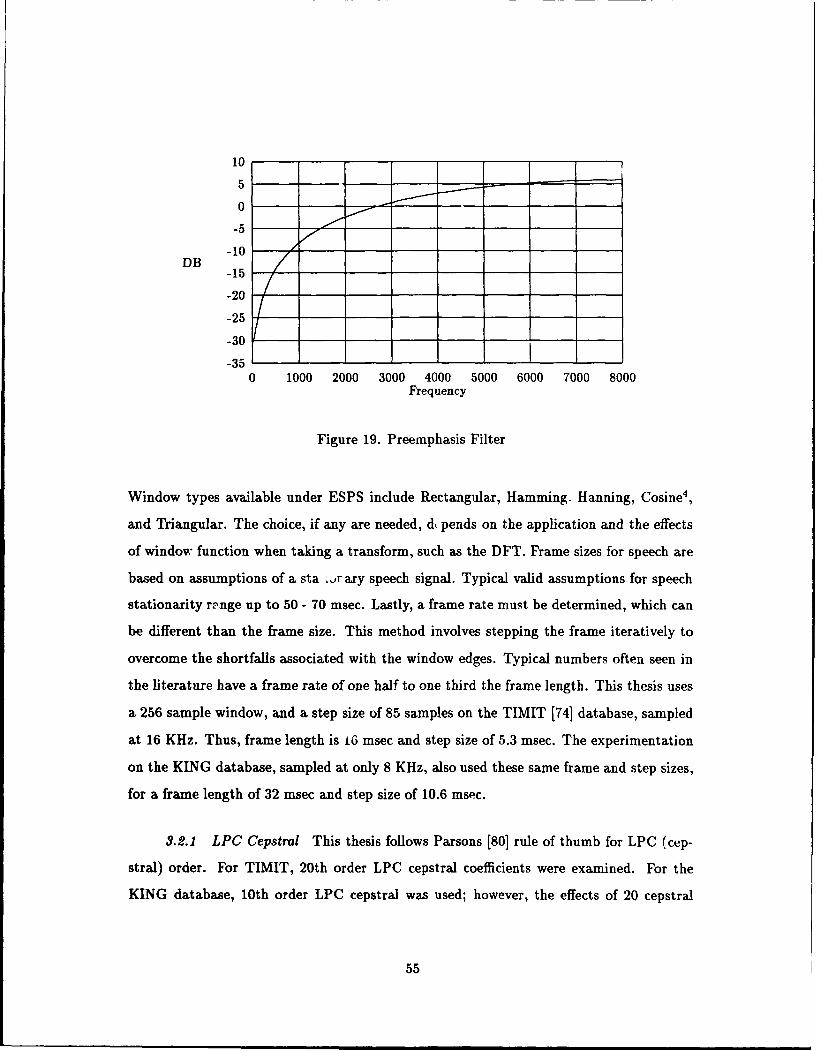
10

5

0

-5 'l

-10

-15

-20

-25

-30

-350 1000 2000 3000 4000 5000 6000 7000 8000

Frequency

Figure 19. Preemphasis Filter

Window types available under ESPS include Rectangular, Hamming. Hanning, Cosine4 ,

and Triangular. The choice, if any are needed, di pends on the application and the effects

of window function when taking a transform, such as the DFT. Frame sizes for speech are

based on assumptions of a sta or ary speech signal. Typical valid assumptions for speech

stationarity rnnnge up to 50 - 70 msec. Lastly, a frame rate must be determined, which can

be different than the frame size. This method involves stepping the frame iteratively to

overcome the shortfalls associated with the window edges. Typical numbers often seen in

the literature have a frame rate of one half to one third the frame length. This thesis uses

a 256 sample window, and a step size of 85 samples on the TIMIT [74] database, sampled

at 16 KHz. Thus, frame length is 16 msec and step size of 5.3 msec. The experimentation

on the KING database, sampled at only 8 KHz, also used these same frame and step sizes,

for a frame length of 32 msec and step size of 10.6 msec.

3.2.1 LPC Cepstral This thesis follows Parsons [80] rule of thumb for LPC (cep-

stral) order. For TIMIT, 20th order LPC cepstral coefficients were examined. For the

KING database, 10th order LPC cepstral was used; however, the effects of 20 cepstral

55

coefficients will be tested. It has been shown that cepstral order greater than LPC order

has improved speech recognition [78].

The LPC Cepstral representation is easily accessible using the ESPS window com-

mand xacf, acoustic feature extraction. This provides an X-Windov interface for the

many parameters needed by the signal processing commands. Each of these features can

also be obtained from the UNIX command line, or through ESPS library programming

support. Such ESPS commands include fit, fftcep and refcof I spectrans -m"CEP"

for representations of DFT, Cepstral(real and complex) and LPC cepstral. The mnethod

used in this thesis, uses the following pipelined ESPS utilities.

filter -Ppreemp.params file.sd- I refcof -P Prefcof-- Ispectrans

-m "CEP" - file.cep

The two parameter files needed are the pre-emphasis filter coefficients and the specific LPC

analysis parameters. The typical pre-emphasis is as follows.

# G(#)preemp.params 1.1 6/3/88 ESI

* parameter file for preemphasis with filter(l-ESPS) program

* for use with lpc analysis .. refcof or lpcana

S

float filter-num = {1.0, -0.97}: "Preemphasis filter numerator";

float filter-den = {1.01: "Preemphasis filter denominator";

int filter-nsiz = 2: "Number of numerator coefficients";

int filter-dsiz = 0: "Number of denominator coefficients";

The specific choice are frame size, step size and LPC procedure is as follows.

S *(O)Prefcof 1.6 3/28/90 ESI

# default parameter file for refcof

int start = 1: "First point to process";

int nan = 0: "Number of points; 0 means continue to EOF";

int frame.len = 256: "Number of points per analysis frame; 0 means nan";

56

int step = 85: "Number or points between start of successive frames;

0 means frame.len";

string window-type = "HAMMING": "Window to apply to data": {"RECT",

"HAMMING", "TRIANG", "HANNING", "COS4"};

int order = 20: "Number of reflection coefficients to compute

per frame)";

string method = "AUTOC": "Analysis method": {"AUTOC", "COV",

"BURG", "MBURG"} ;

Spectral subtraction assumes the noise components are uncorrelated with the speech

signal [80]. When using cepstral coefficients, noise effects can be deemphasized through

a liftering procedure [42]. Bandpass liftering applies a raised sinusoid to the cepstral

representation. The window applied is defined as follows.

w(k) = 1 + (L/2)sin(7rk/L)

where k : (1 < k < L) are the cepstral coefficient index. Juang refers to this procedure

as accentuating formants of the signal. Other liftering techniques include rectangular and

linear windows [42] and filtering temporal aspects of the coefficients, RASTA [46]. It has

been included in the pre-precessing for speaker identification effectively [94, 95] yet, has

also been shown to not improve speech classification [78].

3.2.2 Payton Model The integration of the Payton model with ESPS data struc-

tures can be accomplish through the following method. This chain of pipes demonstrates

the the power of ESPS's implementation of UNIX capabilities.

copysd -s 4000 -d FLOAT infile.sd - I bhd - -I fast I btosps

-f 16000 -n 20 -t FLOAT -c "Payton to ESPS" - outfile.payton

Taking the sampled data (.sd) file infile.sd, copysd will scale the inputs by 4000 and convert

their data type to FLOAT. Typically, ESPS sampled data is SHORT integers. The bhd

function "be-heads" the ESPS header information at the beginning of the file, leaving a

57

Table 5. TIMIT Energy CharacteristicsMinimum Maximum I Average

TIMIT energy 6.87 x 104 1.93 x 106 3.91 x 105

series of raw FLOAT data samples. The single executable, fast, performs all Payton stages

providing as output, 20 channel raw FLOAT data corresponding to auditory nerve firing

rates. An ESPS header is added and this raw data is parsed into outfile.payton, by btosps

- "Binary to ESPS." The number of channels (20), frequency (16 KHz) and comments are

required as parameters for this final function.

It was determined that using TIMIT files directly converted to ESPS sampled data

files (.sd) did not "drive" the auditory model adequately. This can be described as the

model using very quiet or faint speech signals, which would barely cause neural firing

above spontaneous rate. Payton references 0 dB relative to the signal strength necessary

to drive a 1 KHz synapse to threshold, a firing level equal to 10% of the neurons dynamic

range. The dynamic range and threshold for this neuron is shown in Chapter III, Figure

14. Various levels of a 1 KHz sinusoid, ranging from 1 Peak - 3 x 106 Peak level, were

input to the model to determine the RMS values needed to obtain 0 dB. Approximately

75.5 spikes/sec (average) for the 1 KHz synapse required a 2 x 10' Peak sinusoid, with

corresponding RMS energy of 2 x 103.

The subset of TIMIT utterances in these experiments ranged in RMS energy accord-

ing to Table 5. Since conversational speech typically falls into 60 - 70 dB above 0 dB

SPL (hearing threshold), it. was determined to apply an appropriate gain to the TIMIT

utterances before being input to the model. Initial experiments for phoneme recognition

using a gain of 1,000 demonstrated great performance increases [6]. This thesis used a gain

of 4,000 for the TIMIT utterance, placing the average RMS power at 45 dB relative to the

Payton model's reference. The maximum RMS energy utterance then corresponded to a

Payton model reference of 52 dB.

The issue of correct gain for the Payton model was also addressed in the KING

experimentation. Since the KING sessions are separated by "the great divide", RMS

58

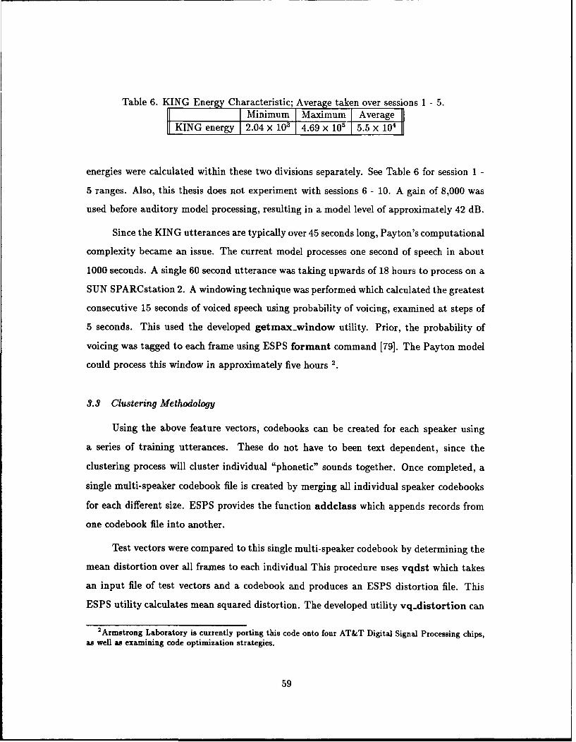
Table 6. KING Energy Characteristic; Average taken over sessions 1 - 5.II1 Minimum Maximum IAverage I

KING energy 2.04 x 10; 4.69 x10 5.5x 10O

energies were calculated within these two divisions separately. See Table 6 for session 1 -

5 ranges. Also, this thesis does not experiment with sessions 6 - 10. A gain of 8,000 was

used before auditory model processing, resulting in a model level of approximately 42 dB.

Since the KING utterances are typically over 45 seconds long, Payton's computational

complexity became an issue. The current model processes one second of speech in about

1000 seconds. A single 60 second utterance was taking upwards of 18 hours to process on a

SUN SPARCstation 2. A windowing technique was performed which calculated the greatest

consecutive 15 seconds of voiced speech using probability of voicing, examined at steps of

5 seconds. This used the developed getmax-window utility. Prior, the probability of

voicing was tagged to each frame using ESPS formant command [79]. The Payton model

could process this window in approximately five hours 2.

3.3 Clustering Methodology

Using the above feature vectors, codebooks can be created for each speaker using

a series of training utterances. These do not have to been text dependent, since the

clustering process will cluster individual "phonetic" sounds together. Once completed, a

single multi-speaker codebook file is created by merging all individual speaker codebooks

for each different size. ESPS provides the function addclass which appends records from

one codebook file into another.

Test vectors were compared to this single multi-speaker codebook by determining the

mean distortion over all frames to each individual This procedure uses vqdst which takes

an input file of test vectors and a codebook and produces an ESPS distortion file. This

ESPS utility calculates mean squared distortion. The developed utility vq.distortion can

2Armstrong Laboratory is currently porting this code onto four AT&T Digital Signal Processing chips,as well as examining code optimization strategies.

59

be used to calculated weighted cepstral, Mahalanobis, root power sums and dot product.

Both commands create an ESPS FEA.DST type file. The command vqclassify will read

this distortion file and present average distortions over the entire sentence and select the

"winning" speaker whose codebook acquired the minimum distortion. Selected portions of

the distortion file, such as source codebook and overall distortion can be easily extracted

using feanprint, allowing further analysis of the speaker distortions in plain ASCII form.

The initial tests on TIMIT were performed training on both sal and sa2 sentences

and quantizing two separate codebooks for each speaker by selecting VOWELS and non-

SILENCE respectively. Varying sizes of these two codebooks were designed at rates of 4

to 9, to examine the stability of identification as a function of codebook size, Figure 20.

Test sentences came from the remaining eight sentences, 5 sx and 3 si per each speaker.

0.08 T r r:Mcm] -:Mefg ---

0.07 ------- -------------- -. hp-• ,, !Mj1s -

0.040 ".0 .. ... ... iiiU

S0.04 - --,0

0.01

1 2 4 8 16 32 64 128CODEBOOK SIZE

Figure 20. Four Speakers Distortio- with varying codebooks, using TIMIT vowels.

Distortions were calculated for these 80 different sentences to the two different codebooks

of four sizes. These 640 total classifications resulted in 100% correctly classified. Figure

21 depicts the typical procedure used throughout this thesis.

The distortion plots in Figure 22 and Figure 23 show an example of the figure of

merit between speaker dependent codebooks. The values are mean distortion per speaker

60

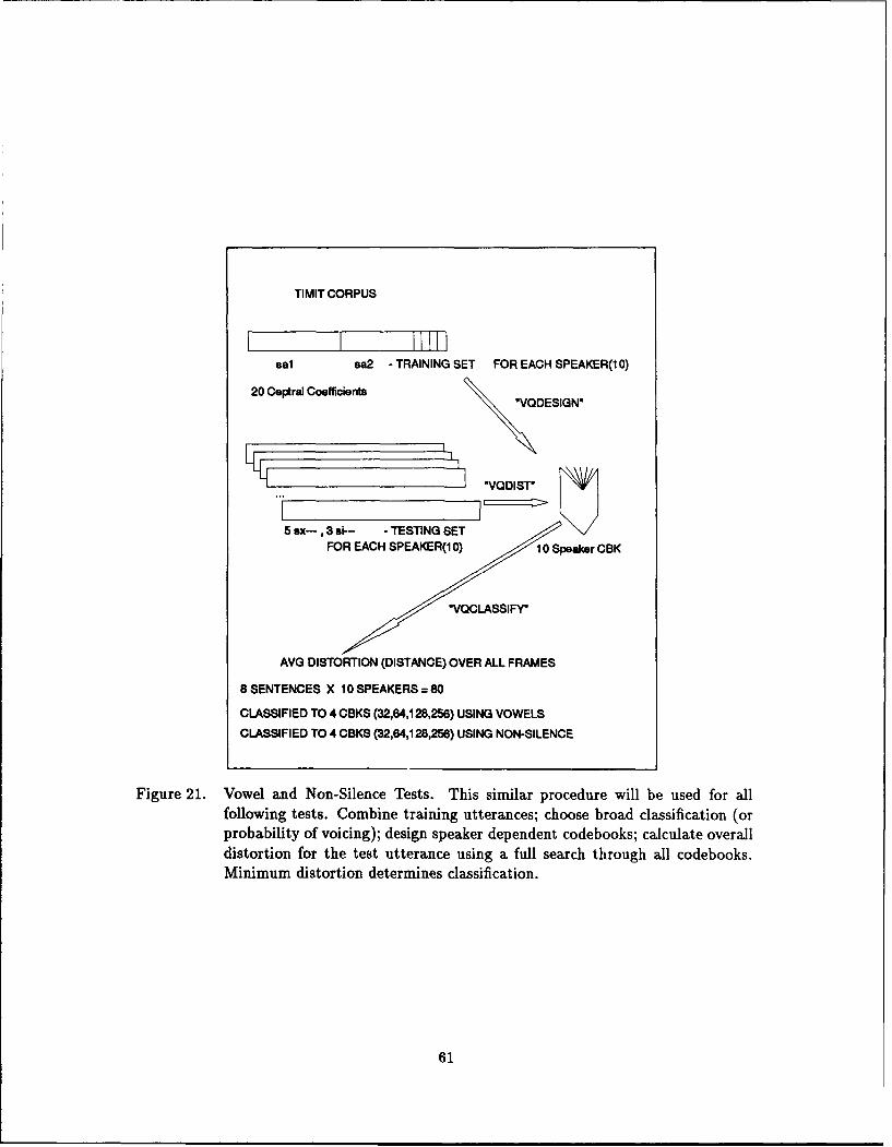
TIMIT CORPUS

sal sa2 - TRAINING SET FOR EACH SPEAKER(10)

20 Ceptral Coefficients "VQDESIGN"

5 sx- , 3 si-- - TESTING SET

FOR EACH SPEAKER(1 0) 10 Speaker CBK

S~"VQCLASSIFY"

AVG DISTORTION (DISTANCE) OVER ALL FRAMES

8 SENTENCES X 10 SPEAKERS= 80

CLASSIFIED TO 4 CBKS (32,64,128,256) USING VOWELS

CLASSIFIED TO 4 CBKS (32,64,128,256) USING NON-SILENCE

Figure 21. Vowel and Non-Silence Tests. This similar procedure will be used for allfollowing tests. Combine training utterances; choose broad classification (orprobability of voicing); design speaker dependent codebooks; calculate overalldistortion for the test utterance using a full search through all codebooks.Minimum distortion determines classification.

61

codebook. The various plots are for the different size codebooks. Notice the relatively flat

distortion values across speakers in Figure 22. This may be attributed to silence and high

frequency noise, such as fricatives or plosives, using codevectors unproductively. Figure

23, however, shows "minimum valleys" clearly corresponding to the correct speaker, when

using only vowels - high probability of voiced speech.

Codebooks of 64 vectors will be used subsequently, as well as extraction of voiced

areas of the utterances for both training and testing. Typical values often seen in the

literature for codebook sizes range from 32 to 256. [45, 46, 68, 113].

A figure of merit used for quantization design is quantization signal-to-noise ratio

QSNR. This thesis examines this ratio to compare the effects of various quantizer pa-

rameters on overall codebook generation. If an original utterance contains N vectors xi,

quantized by ii, then QSNR is calculated as the signal power divided by the quantization

distortion power [127].N 2

QSNR = E (45),=,(X, - j)

As an example, a comparison of QSNR for quantizing TIMIT cepstral coefficients is shown

in Table 7.

Table 7. TIMIT comparison of quantization distortions. TRAINING refers tc the saland sa2 sentences, TEST refers to averaged sx sentences.

male femaleTRAIN TEST TRAIN TEST

Kohonen 12.60 8.93 9.15 9.15LBG 12.52 8.70 9.90 8.27

3.3.1 LBG Design The ESPS command vqdes, provides the LBG algorithm cre-

ating codebooks of sizes 2 ""e, where rate = 1 ... 8 due to the splitting procedure. An

example of the design process with a two dimensional gaussian, standard deviation a = .5

with mean located at (0, 0), is shown in Figure 24.

62

0.08

16 Codewozrds-* 32ý Codewoids---

0.07 .~4 ...... .d . ... . ....* 126Z Codewoilds --

0.06 --. ~.- ~ ---

Uz 0.05 --- ---- -. .... . ......

S 0.04

.. .. . ..

0.0

0.02

0 .0 1 ............. ..... - - -- ---- - - ---

fcVm fcrh fedw -mczj- mefq mhpg mj13 meWh rnprk mrtkSPEAKERS

Figure 22. TIMIT speaker "mcmj" utterance showing distortions to all speaker depen-dent codebooks (LBG) using all speech. Note the low Figure of Merit for thewinning codebook.

0.08 ~16 Codewords -32 Codewords-64 Codewor-ds --

0.0 16 --- ode--....o... ds..

0.02

66

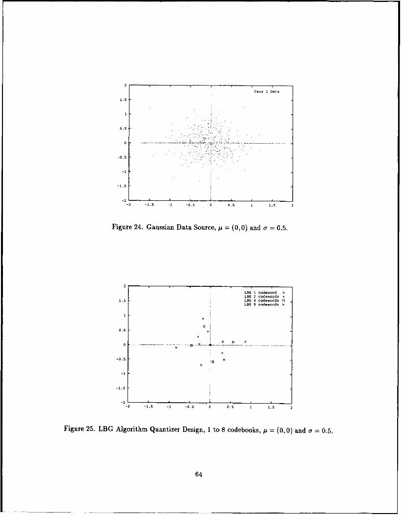
2

Gaus I Data

1.5

0- - - - - 2.. ' -. - .

-0.5

-2-2 -1.5 -1 -0.5 0 0.S 1 1.5 2

Figure 24. Gaussian Data Source, i = (0, 0) and a = 0.5.

2

LBG I codeword *LBG 2 codewords ,

1.5 LBG 4 codewords 0LBG 8 codewords x

1x

00.5 x

X D x

-0.5 x

-1

-1.5

-2 _-2 -1.5 -i -0.5 0 0.5 1 1.5

Figure 25. LBG Algorithm Quantizer Design, I to 8 codebooks, p = (0, 0) and a = 0.5.

64

2

LBG 64 COdewords 0

1.5

1 0

0 0 0

0.5 000

0 0 0 0

00 0 0 0

00. 0 ; 0 0

-0. 00 00

-1 ~000 0

-2-2 -1.5 -1 -0.5 0 0.5 1 115 2

Figure 26. LBG Algorithm Quantizer Design, Final 64 codebooks, it= (0, 0) and a 0.5.Quantization SNR = 15.5 dB.

3.3.2 Kohonen Design Initial Kohonen tests used an 8 x 8 feature map, for fair

comparisons to an LBG 64 vector codebook. The developed ESPS utility vqdesicoh takes

as input an ESPS feature file and outputs a FEANVQ codebook file, using a parameter

file with the Kohonen design specifics. The weights were initialized uniformly to random

values between - .5 and .5. The learning schedule most often used was similar to Figure 28,

developed in AFIT Neural Graphics code [91). The effects of learning iterations on QSNR

is shown in Figure 27.

Examples of the various Kohonen and competitive learning paradigms, using the

data set depicted in Figure 24 are shown in Figures 29, 30 and 31.

The Kohonen design, which maintains neighborhood associations, is shown in Figure

29. Qualitative analysis shows more nodes within regions of higher density. This is in

disagreement with DeSieno's statement [20] that Kohonen learning often models areas of

low density, though a null neighborhood was use in his experiments. It is intuitive that

the neighborhood may pull many more nodes toward dense areas with increased learning

in those areas.

65

26 T

24- - - --

F

-Payton Auditory model

- 20 ---- -- ..... ............. ..... - ..... ....- - - - -

0 16 - - -

. 14H

o 12F

LOC Cepstral

60 50 100 150 200 250 300 350 400 450 500

Kohorien Epochs thru Training Data

Figure 27. Kohonen learning for a TIMIT male(M) and female(F) speaker for varyingiterations (epochs) for LPG cepstral and also Payton. Quantizer "learns"~ inthe first 100 epochs then stabilizes.

"learningschedule -

0.9

0.8

* 0.7

R

7 0.6

0'

'4 0.4

' ~ 0.3

reset at 6 epoch

0.2

reset at 31 epoch

0.1

0 20 40 60 s0 100 120 140 160Kohonen Epoch of Training Data

Figure 28. Kohonen learning schedule

66

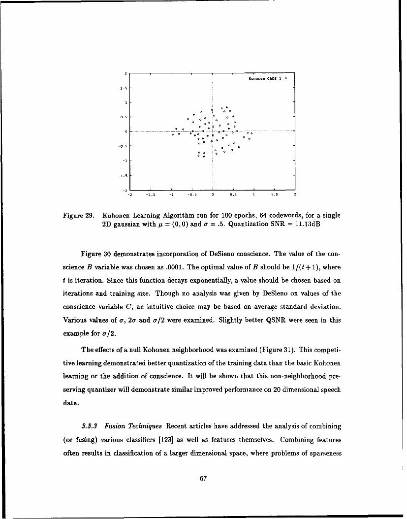
2Kohonen GAUS 1 i

1.5

1

0 00 0 o

00

050 0

•0 • 00 0

0 00 ~ 00

-1

-1.5

-2 I I I I I I

-2 -1.5 -1 -0.5 0 0.5 1 1.5 2

Figure 29. Kohonen Learning Algorithm run for 100 epochs, 64 codewords, for a single2D gaussian with A = (0, 0) and o = .5. Quantization SNR = 11.13dB

Figure 30 demonstrates incorporation of DeSieno conscience. The value of the con-

science B variable was chosen as .0001. The optimal value of B should be 1/(t ± 1), where

t is iteration. Since this function decays exponentially, a value should be chosen based on

iterations and training size. Though no analysis was given by DeSieno on values of the

conscience variable C, an intuitive choice may be based on average standard deviation.

Various values of a, 2a and a12 were examined. Slightly better QSNR were seen in this

example for a12.

The effects of a null Kohonen neighborhood was examined (Figure 31). This competi-

tive learning demonstrated better quantization of the training data than the basic Kohonen

learning or the addition of conscience. It will be shown that this non-neighborhood pre-

serving quantizer will demonstrate similar improved performance on 20 dimensional speech

data.

3.3.3 Fusion Techniques Recent articles have addressed the analysis of combining

(or fusing) various classifiers [123] as well as features themselves. Combining features

often results in classification of a larger dimensional space, where problems of sparseness

67

2

Kohonen Conscience GAUS 1

1.5

1

0

0.5 0 0

00 00° o\ Oo°00 00 ................... . ..... ~...o............- . ......... .% ;'... . ... 0"5" ¢ ' ....................

* o o *0 0, 0 o! 000¢

-0.50 0

0

0 0 0-1

-1.5

-2-2 -1.5 -1 -0.5 0 0.5 1 1.5 2

Figure 30. Same as Figure 29 with DeSieno conscience, conscience parameters B and Cwere .0001 and .1 respectively, for a single 2D gaussian with A = (0, 0) anda = .5. Quantization SNR = 11.32dB.

2

Competitive Learning 0

1.5

0

1 4 00

0 * 0 # 0

0 0

0.5 0 0 0

_ 2 -1 .5 1 0 . 0 0 . 1 .5 2

Fv0

-0. -45 - 0. . 4 .

(0, 0) and a = .5.. Quantization SNR = 15.93dB.

68

can hinder results. Some researchers particularly strive to reduce the dimensionality of the

feature space - such a technique is appropriate choice of Karhunen-Lueve or any principle

component analysis. Xu [123] summaries several techniques concerning combinations of

multiple classifiers. Several of these techniques were examined. For a detailed analysis on

other fusion techniques, see AFIT thesis by Geurts [24'.

3.3.3.1 Probabilistic Classification Currently, Vector Quantization can be used

as a classifier using some given distortion metric. Since the goal is to chose the maximum

likely class i, a ccnversion to distortions from classifier k must be converted to "post-

probabilities." Xu suggests one simple procedure [123].

Pk(i) = 1/dk(i) (46)= 1 1/dk(i)

given M different class distortions, dk(i).

3.3.3.2 Average Fusion The overall fused post-probabilities can then be av-

eraged over all classifiers.1K

PA(i)= E Pk(i) (47)k=1

3.3.3.3 Linear Combination The individual classifiers can be combined be

first appropriately weighting the post-probabilities. A similar technique was examined by

Soong [114] in combining instantaneous and delta cepstral codebook distortions. This was

recently seen in [118].K

Pw(i) = , Wk,,pk(i) (48)k=1

Soong examined the two clssfler case (K = 2) combining normalized distortions.

d(i) = ad( + (1 _ )dA(i) (49)

The denominators are normalization terms which are averaged "intra-speaker distortions."

These weights may be determined by the classification performance of the individual clas-

sifiers [6] or more intuitively, the figure of merit of the ind;vidual classifier distortions. This

69

latter is examined by Geurts [24] given as

Wk. = p + .1(confidence) (50)

where 0 < confidence < 100, which can be related to figure of merit. A slight modification

to this weighting approach uses the inverse of figuro of merit. Defining FOM for class i,

FOMk(i) dk(i) (51)m'niEM{dk(j)}

then,

W,,= 1/FOMk(i) (52)

3.4 Conclusion

This chapter provided the methodology for feature extraction, quantization, and clas-

sification. An initial examination at the recording quality of the two principle databases

sh, ws the contrasting noise levels. Also, examples of quantization distortions on a two

dimensional gaussian source provided insight into the possible effects of Kohonen neigh-

borhood. Classifier fusion techniques were introduced. All signal processing, and data

manipulation were performed using Entropic ESPS functions or developed compatible util-

ities. The following chapter detaiis the recognition accuracies using these quantization and

fusion techniques.

"-70

IV. Experimentation/ Results

Automatic Speaker Recognition experiments were initially performed on a subset of

the speaker corpus contained in TIMIT [74]. Later tests focused on the KING database [59]

which provides a more realistic environment for Air Force applications 1891. Additionally,

AFIT recording were taken for examination of fusion technique with facial imagery. This

chapter examines the recognition results of this data using the methods defined in Chapter

III.

4.1 TIMIT Experimentation

Initial TIMIT classification results demonstrated perfect identification for the ten

speakers using cepstral coefficients, at codebook levels of 32, 64 ,128 and 256 and ,:3ing

either selected VOWELs or non-SILENCE frames. For further tests, varying degrees of

additive white gaussian noise (AWGN) were added to the test utterances. This was accom-

plishied by first creating a gaussian white noise test signal using ESPS testsd then added

this new signal to the original. A typical command for adding an RMS level of noise to 16

KHz sampled data is provided.

testsd -1 RMS.NOISELEVEL -f 16000 -t SHORT file.sd - I

addsd - file.sd noisey.sd

Recognition results were performed for cepstral at SNR levels of 3dB, 10dB, 15dB, 20

dB, 25dB, 30dB, and uncorrupted. Results for the two quantizers are shown in Figure

32. Each provides similar performance, showing the non-generalization of distortion-based

approaches using unprocessed LPC cepstrai coefficients.

For Payton, added white gaussian noise was processed on the test files at the SNR

level of 10 dB only. These results are shown in Table 8 and 9 and compared to cepstral.

This was expected since the training data set was not reprecentative of the test set. Thus,

both feature representations could not generalize tn the added noise.

Lastly, delta coefficients [56], which have been shown to provide uncorrelated infor-

mation to "instantaneous" cepstral were also extracted and quantized. A window of ap-

71

0.9 -- - . 7

Koh~nen ----Sim Anneal -8-

0.8 . ..

0

0.3 -4. . .

0

Ir 0 . 3 -.. . . . . . . .. . . . . .. . .. .-- ,..- - ,-=- -.- . . . .. . . . . . . . . ..... . .. . . ...... ... . ... ... . . .0 . 2 -- -- -....... .... ... ...... .... .... .... . .............. ... ............... . ....... .. . ........ . ......

0.

0 5 10 15 20 25 30 35 40SNR (dB)

Figure 32. Recognition Performance of TIMIT LPC cepstral, using Kohonen SOFM andLinde-Buzo-Gray quantizing algorithms (Simulated Annealing design by Zeger

[127] also shown.) Trained on sal and sa2 sentences, trained on sx.

Table 8. TIMIT Database: Speaker classification. Trained on sal and sa2, tested on sx.Classifier LPC Cepstral Payton Model

Kohonen 100% 76%LBG 100% 90%

proximately 100 msec [114] ( ±8 TIMIT frames) was used for the delta operation. These

results are shown in Table 10.

This section provided the initial procedures which will further be examined on the

KING corpus. Current speaker recognition researchers prefer the KING database. The

recordings are not prompted; the long distance telephone characteristics are dynamic; the

recording equipment quality changed drastically after half the data base was obtained, and

the multiple sessions capture varying intra-speaker distortions.

The key aspects learned from initial TIMIT experimentation are as follows. LPC

cepstral, the proven technique performs perfectly (i.e. 100% classification) in clean speech.

It also drops greatly in increasing noise environments. While the Payton model did good

72

Table 9. TIMIT Database: Speaker classification. Trained on sal and sa2, tested on sxwith 10dB AWGN.

Classifier LPC Cepstral Payton ModelKohonen 16% 22%LBG 9% 30%

Table 10. TIMIT Database: Speaker classification. Delta coefficients using an approxi-mate 100 msec window (± 8 frames). Trained on sal and sa2, tested on sx.

Classifier LPC Cepstral Payton ModelKohonen 64%b 22%LBG 94% 66%

(90% using LBG) for clean speech, it's performance still dropped markedly. The informa-

tion contained in delta (transitional) representations contains speaker dependent informa-

tion. The Kohonen SOFM consistly performed below that of the classic LBG algorithm.

This can probably be explained by the neighborhood process, which has demonstrated

this effect on 2D gaussian data sets. Though Kohonen learning has been referenced as a

means to avoid local minima, an incorrect neighborhood may "pull" nodes to more dense

regions of the probability density function, resulting in poor "tail" modeling. Also, a two

dimensional lattice (neighborhood structure) may not be suitable for these particular test

sets. Though results not provided, supervised learning provided by Learning Vector Quan-

tization, distorted class boundaries resulting in slightly decreased QSNR's. Since averaged

distortion is used for classification, as opposed to single frame nearest neighbor, LVQ did

not provide increased recognition.

4.2 KING Experimentation

4.2.1 10 Class Tests Results obtained are shown in the following tables. Table 11

will be used as the baseline performance for the 10 speaker tests. Additional quantizers

using conscience and 3D Kohonen "lattice" were examined. The recognition performance

did not improve greatly with these techniques. The parameters of conscience used were

73

Table 11. KING Database: Speaker classification. Trained on sessions 1 - 3, tested onsessions 4 and 5; 10 speakers.

Classifier LPC Cepstral Payton ModelKohonen 55% 20%LBG 80% 70%

B = .0001, based on DeSieno's [20] work, and a parameter C based on average standard

deviation of the training vectors. The three dimensional Kohonen uses a, 4 x 4 x 4 cube,

with 3D radial neighborhood. The use of the incremental Kohonen learni ag without neigh-

borhood will be examined and referred to as "Competitive Learning." Slight improvement

over Kohonen learning has been demonstrated with this technique, shown with .95 and

.5 initial learning rates. Other parameters of the Kohonen learning remained unchanged.

Results are shown in Table 12.

Table 12. KING Database: Speaker classification. Trained on sessioils 1 - 3, tested onsessions 4 and 5, Kohonen Modifications; 10 speakers.

Classifier LPC Cepstral Payton ModelKohonen w/ Conscience 55% 25%Kohonen 3D 4x4x4 50% 40%Competitive (.95) 63.3% 40%Competitive (.5) 55.0% 60%

The effect of varying probability of voicing changes recognition slightly for LBG

quantization. The ESPS formant command, based on Secrest and Doddington's [79, 107]

pitch tracking algorithm, often assigns a very small (< .1) or very large (> .9) probability

of voicing value. Thus, the additional number of frames changed marginally by using low

probabilities for training. These extra frames (typically on voiced-unvoiced boundaries)

may have aided Kohonen's incremental learning in spreading out of dense codebook areas.

See Table 13.

The effects of Payton normalization schemes and Kohonen training are shown Tables

14 and 15 respectively. Normalization did increase performance for the Payton model.

74

Table 13. KING Database: Speaker classification. Trained on sessions 1 - 3, tested onsessions 4 and 5. Probability of Voicing Influence on the Payton Model; 10speakers.

Classifier .1 PV .3PV .5 PV .7 PV .9 PVKohonen 40% 30% 30% 30% 20%LBG 70% 80% 70% 70% 80%

Performing a zero mean across vector elements of auditory vectors has been seen in the

literature [32].

Table 14. KING Database: Speaker classification. Trained on sessions 1 - 3, tested onsessions 4 and 5. Normalization Influence on the Payton Model.

Classifier Remove Mean/Feature Zero Mean VectorsKohonen 30% 35%LBG 60% 85%

Table 15. KING Database: Speaker classification. Trained on sessions 1 - 3, tested onsessions 4 and 5. Kohonen Training Time Influence on the Payton Model.

Classifier I40 Epochs 1120 Epochs I250 EpochsKohonen 20% 50% 50%

A series of delta coefficients, as reviewed in Section 2.2.2.5 were extracted from the

KING instantaneous cepstral vectors. No documentation has been reported on successful

use of temporal characteristics on the KING narrowband corpus. Again for cepstral, a

100 msec window was used [114], resulting in a ±4 frames in calculating the new coeffi-

cients for the cepstral coefficients. Performance increases over instantaneous cepstral were

demonstrated. A series of delta windows were examined for the Payton model, shown in

Figure 33. This new technique for the auditory model captures temporal firing informa-

tion without specifically calculating neural pulse trains. Since it has been shown that delta

cepstral contains uncorrelated information to that of instantaneous cepstral, this technique

75

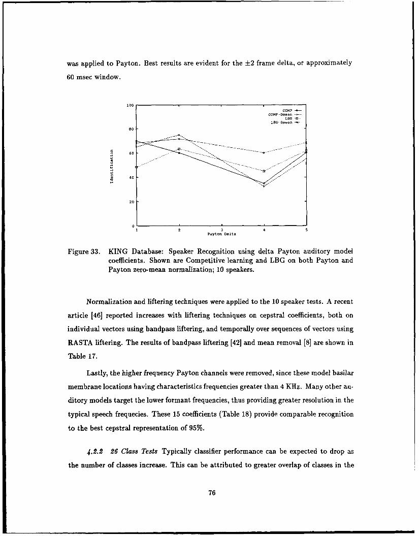
was applied to Payton. Best results are evident for the +2 frame delta, or approximately

60 msec window.

100COMP

COMP-OmeanLBG - -

LBG- Omean -k.-

80

o 60 -" . ... -- " --. . . . . "

20

-.4. -'. " "": -.... " °

0 40

20

1 2 3 4Payton Delta

Figure 33. KING Database: Speaker Recognition using delta Payton auditory modelcoefficients. Shown are Competitive learning and LBG on both Payton andPayton zero-mean normalization; 10 speakers.

Normalization and liftering techniques were applied to the 10 speaker tests. A recent

article [46] reported increases with liftering techniques on cepstral coefficients, both on

individual vectors using bandpass liftering, and temporally over sequences of vectors using

RASTA liftering. The results of bandpass liftering [42] and mean removal [8] are shown in

Table 17.

Lastly, the higher frequency Payton channels were removed, since these model basilar

membrane locations having characteristics frequencies greater than 4 KHz. Many other au-

ditory models target the lower formant frequencies, thus providing greater resolution in the

typical speech frequecies. These 15 coefficients (Table 18) provide comparable recognition

to the best cepstral representation of 95%.

4.2.2 26 Class Tests Typically classifier performance can be expected to drop as

the number of classes increase. This can be attributed to greater overlap of classes in the

76

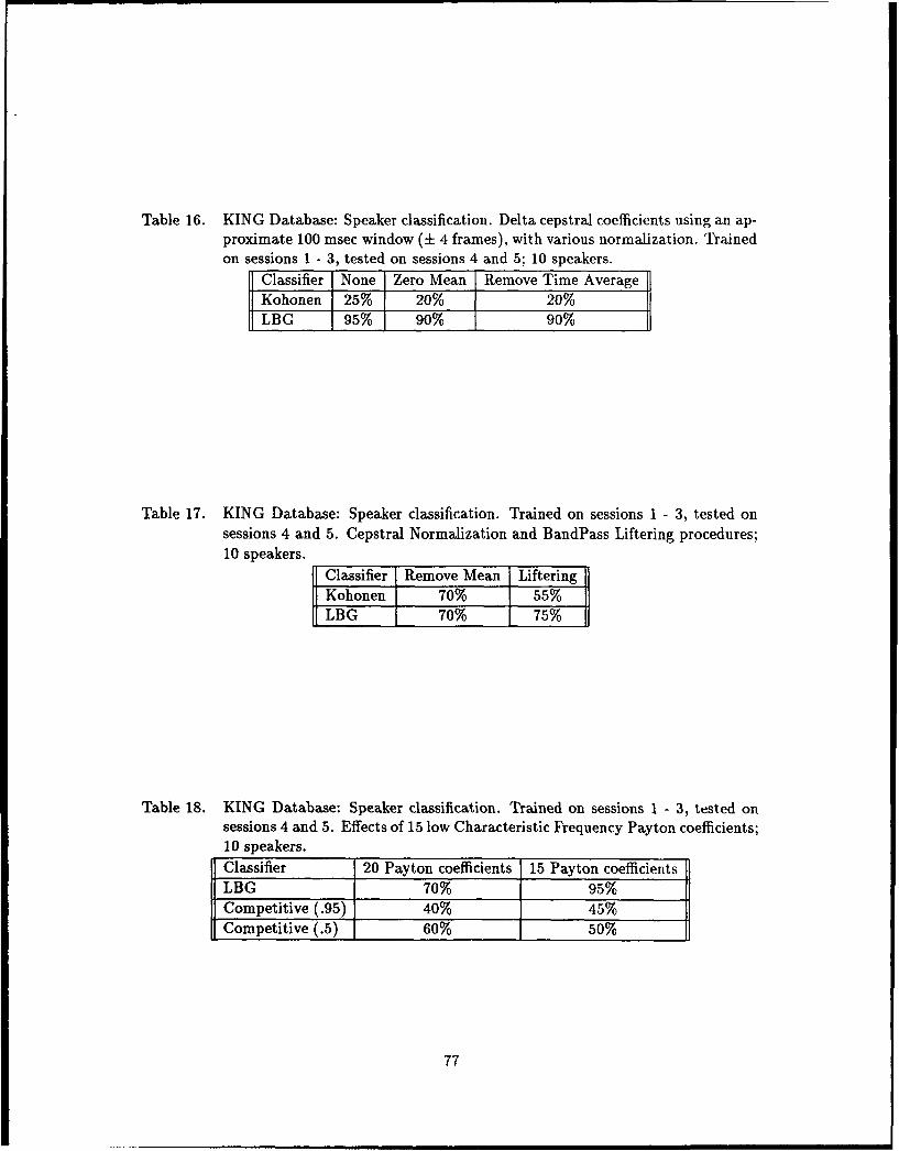
Table 16. KING Database: Speaker classification. Delta cepstral coefficients using an ap-proximate 100 msec window (± 4 frames), with various normalization. Trainedon sessions 1 - 3, tested on sessions 4 and 5; 10 speakers.

Classifier None Zero Mean Remove Time AverageKohonen 25% 20% 20%LBG 95% 90% 90%

Table 17. KING Database: Speaker classification. Trained on sessions 1 - 3, tested onsessions 4 and 5. Cepstral Normalization and BandPass Liftering procedures;10 speakers.

Classifier Remove Mean LifteringKohonen 70% 55%LBG 70% 75%

Table 18. KING Database: Speaker classification. Trained on sessions 1 - 3, tested onsessions 4 and 5. Effects of 15 low Characteristic Frequency Payton coefficients;10 speakers.Classifier 20 Payton coefficients 15 Payton coefficientsLBG 70% 95%Competitive (.95) 40% 45%Competitive (.5) 60% 50%

77

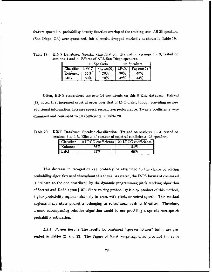
feature space; i.e. probability density function overlap of the training sets. All 26 speakers,

(San Diego, CA) were quantized. Initial results dropped markedly as shown in Table 19.

Table 19. KING Database: Speaker classification. Trained on sessions 1 - 3, tested onsessions 4 and 5. Effects of ALL San Diego speakers.

10 Speakers 26 SpeakersClassifier LPCC Payton(0) LPCC Payton(O)Kohonen 55% 20% 36% 40%

LBG 80% 70% 42% 44%

Often, KING researchers use over 14 coefficients on this 8 KHz database. Paliwal

[781 noted that increased cepstral order over that of LPC order, though providing no new

additional information, increase speech recognition performance. Twenty coefficients were

examined and compared to 10 coefficients in Table 20.

Table 20. KING Database: Speaker classification. Trained on sessions 1 - 3, tested onsessions 4 and 5. Effects of number of cepstral coefficients; 26 speakers.

Classifier i10 LPCC coefficients 20 LPCC coefficients

Kohonen 36% 54%

LBG 42% 60%

This decrease in recognition can probably be attributed to the choice of voicing

probability algorithm used throughout this thesis. As stated, the ESPS formant command

is "related to the one described" by the dynamic programming pitch tracking algorithm

of Secrest and Doddington [1071. Since voicing probability is a by-product of this method,

higher probability regions exist only in areas with pitch, or voiced speech. This method

neglects many other phonetics belonging to voiced areas such as fricatives. Therefore,

a more encompassing selection algorithm would be one providing a speech/ non-speech

probability estimation.

4.2.3 Fusion Results The results for combined "speaker-listener" fusion are pre-

sented in Tables 21 and 22. The Figure of Merit weighting, often provided the same

78

results to that of average weighting. Also, the final classification correlates to the highest

attainable level by the single best classifier alone. This was true for both the 10 speaker

and 26 speaker tests (Table 23).

4.2.4 Speaker Verification A series of codebooks were designed to perform speaker

authentication/ verification. Typically, a single speaker dependent codebook is created

per speaker and thresholds are varied to evaluate verification performance. An extension

to this procedure uses two separate codebooks for each individual. The first uses speaker

dependent speech. The second uses speech from a set of targets. For KING, speakers 1 -

13 were used as targets, and speakers 14 - 26 were used as imposters. A similar method of

testing was documented by TI [46]. The results are shown in Table 24.

The two features used, cepstral and Payton (zero mean normalization) demonstrated

overall equal performance of 88% correct classifications. However, still note the exception-

ally high false acceptance rate.

4.2.5 Feature Analysis The effects of normalization improved classification perfor-

mance for Payton by 15%. This zero mean normalization has been seen in the literature

[32] as well as performed on speech recognition experiments in AFIT theses by Stowe [115]

and Recla [87]. This normalization effect on codebook generation may be explained on the

basis of the Fisher ratio. The Fisher ratio (F-ratio) is a general figure of merit used for

feature selection. Parson [80] describes this as "the variance of means over the mean of

the variances", assuming a set of training data which can described (clustered) by class.

In generalizing speaker dependent codebooks for Parson's training data, a similar Fisher

ratio can be developed. This not only provides a measure of the feature representation to

separate classes, but may also provide insight into the quantizer design process. Typically,

the greater the F-ratio, the better the representation. This application can be described as

a measure of inter-speaker class separation over the intra-speaker class compactness. The

formulation is,

79

Table 21. KING Database: Speaker classification. Average and Figure of Merit (FOM)Fusion. Note - PAM is Payton Auditory Model, LPCC is LPC cepstral and(0) represents zero mean normalization; 10 speakers.

Classifier Average Fusion FOM FusionLPCC + PAM 80% 80%LPCC + PAM(0) 85% 80%LPCC + ALPCC 85% 85%PAM + APAM 75% 75%PAM(0) + APAM(0) 75% 70%ALPCC + APAM(0) 90% 90%

Table 22. KING Database: Speaker classification. Average, Figure of Merit (FOM) andWeighted Fusion. Note - PAM is Payton Auditory Model, LPCC is LPC cep-stral and (0) represents zero mean normalization. WEIGHTED uses the recog-nition accuracy of the individual classifiers for weights in fusion; 10 speakers.

Classifier Average FOM WEIGHTEDLPCC + PAM + ALPCC + APAM 90% 90%LPCC + PAM(0) + ALPCC + APAM(0) - 95%

Table 23. KING Database: Speaker classification. Average and Figure of Merit (FOM)Fusion. Note - PAM is Payton Auditory Model, LPCC is LPC cepstral and(0) represents zero mean normalization; 26 speakers.

Classifier I Average Fusion FOM FusionLPCC + PAM(0) 50% 50%

Table 24. KING Database: Speaker Authentication. Trained on sessions 1 - 3, tested onsessions 4 and 5; 13 Targer speakers, 13 Imposters.

Classification LPC Cepstral Payton ModelFalse Reject 27.0% 58.0%False Accept 11.0% 8.88%True Accept/Reject 88.0% 88.0%

80

F= =D =l(s,.d - f)(53)1 ES °__, Il= °8=1 K d=l(Ckd - 11sd)

where S = number of speakers,

K = number of codewords per speaker codebook,

D = dimension of codewords,

/l,,d = d dimension of s speaker mean,

•d = d dimension of global mean of all S speaker means,

and C5,k,d = d dimension of s speaker's k codeword.

Table 25 examines severai F-ratios on the generated speaker codebooks. The increased

figure of merit for the normalized coefficients is the result of a reduced denominator in

Equation 53, caused by a reduced average variance per speaker. Note also that Kohonen

quantization always produced a slightly higher F-ratio than LBG. This factor is due to a

consistently smaller denominator, than that of LBG, possible caused by Kohonen nodes

maintaining locations within relatively dense areas of the training set.

Table 25. KING Database: Speaker dependent codebook evaluation with Fisher Ratio[80]

Test Case LPC Kohonen LPC LBG PAM Kohonen PAM LBG10 Speaker Baseline .566 .382 .416 .260Delta 10 Speaker .109 .048 .055 .077Zero Mean 10 Speaker - - .475 .331

Delta Zero Mean - - .104 .062

Remove Mean .0927 .0736 .210 .091Delta Remove Mean .109 .048 .074 .044

Examination of the Payton and cepstral vectors and individual channels (coefficients)

for speaker separability was performed; see Figures 34 and 35. Distortion histograms

for individual coefficients provided little insight to class separability. The separability of

speakers is evident only by averaged distortion over many frames. The goal was to account

81

0.0 1INTRA CEP -INTER CEP

0.07

0.06

0.05

0 0.04

0.03

0.02 ,.

0.01

0 L \~.

0.1 0.2 0.3 0.4 0.5 0.6 0.7 0.8 0.9Distortion

Figure 34. Cepstral Speaker Separability: KING Database: Normalized Histogram ofInter speaker and Intra speaker distortions using three speakers, over foursessions. F-ratio = 0.515

0.08INTRA PAYTON -INTER PATTON --

0.07

0.06

0.05

0.04

0.03

0.02

0.01

0 0.1 0.2 0.3 0.4 0.5 0.6 0.7 0.9 0.9Distortion

Figure 35. Payton Speaker Separability: KING Database: Normalized Histogram of Interspeaker and Intra speaker distortions using three speakers, over four sessions.F-ratio = 0.124

82

for potentially improved distortion metric than Euclidean. If certain coefficients could

individually separate speakers, these could be used with a particular weighted metric.

Overall intra-speaker and inter-speaker distortion histograms re shown for cepstral and

Payton (zero mean normalized). The F-ratio between the two classes (inter-speaker and

intra-speaker) is given by .515 for cepstral and .124 for Payton.

4.3 AFIT Corpus Experimentation

A concept of "user identification" is being developed which fuses the benefits of

both face recognition and speaker verification. This system is envisioned to simultaneous

capture facial imagery and require a name or text independent speech samples. Initial

speech characterization is provided.

4.3.1 Recording Setup Training and testing was performed for both speaker iden-

tity (name) and high phonetical content sentences acquired from the TIMIT Continuous

Phonetic Speech Database. A series of four prompted MIT sx sentences, two speaker name

recording and another speaker name were recorded for ten speakers over a ten day pe-

riod. The utterances were captured using Entropic Research Laboratory's ESPS pack'age,

specifically using the Ariel PRO-Port Model 656 Stereo A/D Converter. The ESPS com-

mand s32crecord has been used, with a 16 kHz sampling rate and 16 bit linear coding

(SHORTs). A 20th order LPC analysis converted to 20 LPC cepstral coefficient was per-

formed using ESPS refcof and spectrans functions. The speaker ames werq also processes

through the Payton auditory model, then mean rate response was calculated on 16 msec

frames at a frame rate of 5.33 msec. Speakers are represented by codebooks created using

the LBG algorithm using 64 codewords per speaker.

4.3.2 Recognition Results Identification tests were performed by training on either

the phonetically balanced (PB) sentences or the speaker names (SN). Testing used either

the PB, SN and also the other name utterances. These other names will be used for

imposter (IM) verification. Identification results used increasing training sessions and

testing on several latter days are provided in Table 26. For example, when examining

the Day 6 entries, codebooks were created using all utterances recorded over 6 days, and

83

testing consisted of utterances from Days 7 - 10. Separate codebooks were created for the

PB and SN utterances per speaker. For the Payton representation, only speaker names

(SN) were processed. This demonstrates how increased sessions used in training consistly

Table 26. AFIT User Identification Database: Speaker Identification using PhoneticallyBalanced and Speaker Names. Trained over increasing number of days, Testedon several following days; 10 speakers.

Training Time 1 Day 2 Days 3 Days 4 Days 5Days 6 Days 7 DaysPhonetically Balanced 91.87 94.16 96.25 97.5 98.75 99.16 100.0Speaker Names 92.85 98.33 97.5 95.0 100.0 98.33 97.5

Speaker Names (Payton) 1 76.50 92.30 96.32 97.41 98.95 98.75 98.33

improved identification. Since the PB sentences each contain rich phonetic content, it

can be inferred that both diversive phonetic frames and many intra-speaker exemplars of

these frames over multiple sessions increase identification accuracy. Increased multi-session

training sets have also shown to increase face recognition performance, demonstrated in

AFIT thesis by Krepp [54]. Note in Table 27 the performance of another's name by an

imposter speaker is recognized consistently by the PB codebook, yet is often in error by

the SN codebook. This is explained by the rich phonetic content of the training set, when

using PB (TIMIT sx) sentep-es. These have been plotted for comparison in Figure 36.

Table 27. AFIT User Identification Database: Speaker Identification using other names.Trained over increasing number of days, Tested on several following days. Sametest procedures as Table 26. Other Name (Imposter) recordings were tested onboth the PB and the SN codebooks; 10 speakers.

Training Time 1 Day 2 Days 3 Days 4 Days 5Days 6 Days 7 DaysImposter on SN 30.0 53.3 45.0 40.0 64.0 67.5 70.0Imposter on PB 87.5 96.7 100.0 100.0 100.0 100.0 100.0

Speaker verification was performed using the method of "Me" and "Not Me" code-

books outlined in Section 4.2.4. Verification was performed for the Speaker "skr" SN

codebook while testing on utterances by all 10 subjects stating "skr"'s name. Tests were

examined over codebooks designed using increasing training session for the cepstral co-

84

efficients only; see Figure 37. Figure 37 demonstrates how the PB sentences provide

better verification (0% false reject, 1.66% false accept) than speaker names (6.6% false

reject ,11.1% false accept) after 5 training sessions. Also, the imposters using speaker

names, even over multiple training days, show more variance in testing accuracy than the

phonetically balanced sentences.

4.4 Conclusion

This chapter investigated the use of TIMIT, KING and AFIT recorded databases

and the effects of both traditional and neural feature representations using both LBG and

Kohonen quantizer design algorithms. The following chapter provides analysis of these

results and provides overall conclusions.

85

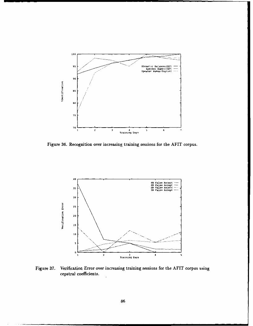
100

95 Phon~etic Balance(CE1P)|,,-'° • ... "'" peaker Names (CEP) ..

90

0

85

80

75

701 2 3 4 5 6 7

Training Days

Figure 36. Recognition over increasing training sessions for the AFIT corpus.

40

PB False Reject -

PB False Accept35 SN False Reject -----

SN False Accept -

30

0S254.220I-

1220

>

10

5 .. .. .. ....

-- -- ------

12 3 4 5Training Days

Figure 37. Verification Error over increasing training sessions for the AFIT corpus usingcepstraJ coefficients.

86

V. Conclusions/ Final Analysis

This thesis compared the current proven LPC cepstral representation to features

provided by the Payton auditory model, on a variety of speech databases. Recognition

accuracies were compared using Linde-Buzo-Gray and Kohonen Self Organizing Feature

Map quantizer designs. The final comparative analysis, overall, is that the two represen-

tations achieved similar results. For example, in 10 speaker KING tests, equal accuracies

of 95% can be achieved. Similarly, for the AFIT corpus, both representations for speaker

name identification achieved upwards of 98% recognition. The reduced recognition of the

Payton model on TIMIT by 10% may be the highly efficient representation of LPC cep-

stral in clean conditions. Several noteworthy conclusions have been theorized during this

effort concerning specific aspects of the quantization design, normalization techniques and

preprocessing techniques and Payton auditory model implementation.

5.1 Quantization Design/ Classification

Kohonen SOFM consistently provided inferior recognition accuracies than that of

LBG. Also, competitive learning demonstrated slightly better recognition results to that

of Kohonen. This became evident after much "trial-and-error" experimentation of Ko-

honen parameters, as well. Kohonen conscience and a 3D Kohonen lattice provided no

improvement, and these techniques also currently require a similar adhoc approach to pa-

rameter choice. Similar performance in comparing Kohonen with LBG (and other neural

quantization technique) was demonstrated by Wu [122].

Past AFIT research by Recla and Stowe [87, 115) only investigated recognition by

using the feature map neighborhood preservation qualities. These authors incorporated

the speech trajectories through the Kohonen feature map with dynamic programming tech-

niques for speech recognition. Since, overall distortion was used for speaker recognition in

this thesis, neighborhood preservation was not beneficial or required. The desired quantizer

design was the optimal non-parametric model of the training speech.

Quantizer design is a simple non-parametric approach to modeling the underlying

probability density function of the speaker training data. It was recently reported by

87

Lippmann [61] that many parametric, neural and non-parametric approaches to class pdf

estimation provide similar results. The underlying differences are peripheral, such as speed,

memory, training time, testing time and storage requirements. Thus, a number of other

techniques could have been tried and performance should have been similar. The TIMIT

tests clarified the inability of this technique to generalize in added white gaussian noise

(AWGN), with recognition rates dropping from 90 - 100% for Payton and cepstral in

clean representations to below 30% in 10 dB AWGN. Payton did provide nearly twice the

recognition accuracy of LPC cepstral for this series of AWGN tests.

Successful fusion techniques have been demonstrated when differing features can be

extracted [87, 115]. Likewise, fusion of classifiers has been demonstrated [24, 123] and may

prove more efficient for increased speaker tests. One concern should always be increased

dimensionality, which typically increases sparseness within the feature space [91]. Increased

recognition was not demonstrated over the best individual classifier. Further analysis on the

issue of "user identification" fusion is beginning. This thesis examined fusing information

between a speaker model (cepstral representation) and a listener model (auditory features)

for recognition. However, the common base between these are the same samples of data.

When corrupted, reductions should be seen in both spectral representations. The ability

to fuse different representations, such as speech and face imagery, with no common base of

information except user identity, could be envisioned as an improved "user identification"

system.

Though differenced or delta coefficients were examined within the VQ framework,

improved recognition may be evident using models better suited to extract temporal in-

formation. These would include recurrent neural networks or the popular Hidden Markov

Models. The underlying assumption of this thesis was the evidence of speaker dependent

information, available through examination of instantaneous feature vectors or their tem-

poral characteristics. Recent research from AT&T shows instantaneous cepstral providing

better recognition than delta cepstral [118]. Based on efforts within this thesis, this tran-

sitional information may have characteristics based on speech corpus recording quality or

content.

88

5.2 Preprocessing

Normalization is always an important step in typical neural processing and classifica-

tion. The effects of statistical normalization, removal of long term averages, insuring each

vector has zero mean (across elements) as well as energy normalization have each been

examined on the Payton auditory vectors. Using the LBG algorithm, performing a zero

mean normalization attained 85% recognition for Payton, and further reduction of vector

dimension to 15 coefficients attained 95% recognition.

Liftering provided no significant improvements on the 10 or 26 class KING tests. This

procedure, typical of filtering in the cepstral domain, can be regarded as a de-emphasis

of certain coefficients. In bandpass liftering, this procedure attenuates the low and high

order coefficients. Alternatively, a weighted Euclidean distortion metric could be used.

Examination of a form of neural spectral subtraction was performed on the TIMIT AWGN

tests, yet no improvements can be reported. A type of emphasis (like band-pass liftering)

may be done on the raw speech before input into the model to compensate for broad outer

ear effects [103, 112]. The Payton coefficients were examined for their saliency [97] to

provide inter-speaker separation. Histograms of inter-speaker and intra-speaker codebook

distortions were examined, yet coefficients individually provided no class separability. Only

when using the average distortion over an ensemble of vectors did separability become

evident.

Lastly, temporal filtering on the cepstral vectors may have an analogy when examin-

ing the temporal aspects of the nerve firing. This thesis examined the average rate response

over windows for speaker dependent information. Likewise, it has been shown in physi-

ological data on cats that synchrony information is a more robust neural representation

than average rate response [100, 125]. The delta representation examined the temporal

aspects of neural firing for speaker identification. Recognition of 95% using delta cepstral

and 80% using delta Payton has been shown. Additionally, the final Brachman stage of

Payton transduction stage could be developed to provide neural pulse trains, as opposed

to the predicted firing rates. Phase synchrony representations of the neural model may

provide detailed frequency dependencies among the 20 Payton channels or with various

fundamental frequencies.

89

The drastic drop in classification for the 26 speaker corpus can be explained by

several factors. Typically, KING researchers use the entire 45 to 60 second utterances

for both training and testing. The effects of training time and testing time greatly effect

vector quantization procedures. Due to the described Payton computational complexity, a

15 second window with maximum voicing was extracted for further model processing. The

cepstral representation, to be fairly compared with Payton, required equal windowing.

However, much of the 15 second window was not voiced speech, since the database is

conversational in nature. Training times varied greatly from about 600 to 1500 frames of

data, corresponding to about 6 to 15 seconds total, whereas other researchers typically use

90 seconds of training data. Likewise, testing time for a window averaged 379 frames of

voiced speech or about 4 seconds, whereas comparable work would could use 30 seconds for

testing. For example, a session containing 3993 frames (10.63 msec frame rate) of speech

only resulted in 1100 frames with a voicing probability greater than 0.1.

Using a different set of probability of voicing parameters or another means of calcu-

lating these values would increase training and test sets. Additionally, the phonetic content

of the speech, both in training and testing extraction was limited to high voiced regions,

not encompassing a rich phonetic balance. Speaker classification has been shown to be

correlated to the phonetic content of the training set [113]. For clean data, such as the

TIMIT recordings, perfect classification using cepstral was evident using either VOWELS

(high probability of voicing) or non-SILENCE (any speech regions). For degraded signals

such as KING, these other phonemes may add additional information.

5.3 Auditory Modeling

The Payton model differs from several other popular models by modeling the biologi-

cal processes as opposed to their characteristics. This model provides non-linear responses

to increased stimulus levels. The background efforts of this thesis have provided the de-

tails to fully understand this particular models' parameters, assumptions and limitations.

The Payton model, like all others, models a far reduced set of channels than physiolog-

ically evident. The approximately 2500-3000 inner hair cells are a measure of spectral

resolution. However, many physiological issues remain which should guide future research.

90

Through nonlinear biological processing, various saturation, rectification and adaptation

occur between these inner hair cell depolarizations and the auditory nerves they synapse.

Is the vast number of 25,000 - 30,000 auditory nerves for redundancy or to enable further

processing? Higher cortical speech processing has begun to be investigated [55]. On the

auditory cortex, finer resolution indicates a potential lateral inhibition of neural signals

among these auditory nerves. Also, the knowledge that both theories of pitch perception

are active for speech based frequencies can guide future work to develop techniques which

use both spectral analysis and temporal phase information for the recognition process.

The issue of correct input scale is very necessary and sensitive in auditory modeling

(6]. While the ensemble set of auditory nerves have a dynamic range of 120 dB, as evident

from Fletcher-Munson curves [80], individual neurons only have a 30 dB range of firing.

This thesis has chosen a scale so the average firing for the reference 1 KHz CF neuron

is 40 - 50 dB above the model reference level. This puts the model in the overall range

of low to moderate speech levels. Instantaneous firing of individual Payton channels still

saturate. Such physiological explanations of automatic gain control have been theorized

as functionality of the outer hair cells, yet their contribution to the transduction process

is still not known.

Payton processing greatly limited the amount of data which could have actually been

incorporated. The entire KING database of 51 speakers and 10 sessions per speakers would

have taken upwards of 9180 hours or over 12 months to completely process. However,

by taking a 15 second window, the results reflect the limitations of this method. Like

many other techniques, such as Hidden Markov Models, adequate training data becomes

critical. Results for this amount of data on KING, for the 26 speaker tests, provides a

relationship to the speaker density function overlap. Additional training data would have

enabled improved speaker pdf estimations and additional phonetic content. This would

'inevitably increased recognition, as evidence from recent published data on KING, using

similar codebook design strategies.

The current model trades computation cost (160,000 Fourier-Inverse Fourier Trans-

forms/ second) for physiological precis*-•n. Engineering dictates trade-offs. Average rate

response was examined in this thesis and other models may provide adequate charac-

91

teristics with much lessing processing. This could allow investigation of further feat lire

preprocessing, such as synchrony, correlations, lateral inhibition, etc. Initial results of

auditory modeling, for speech and speaker recognition applications, are still developing.

Questions concerning tVe benefits of non-linear spectral processing and effects of auditory

periphery characteristics toward improved recognition need still be addressed.

92

Appendix A. Human Auditory Physiology

For many years, psychoacoustic experimentation was based on simple stimulus, such

as single tones and clicks. Only recently has data been published on auditory nerve patterns

in response to complex signals such as sums of sinusoids and synthetic speech. Several

models have been created which attempt to model this physiological data. Attempts

have also been reported using an auditory model as a preprocessor for speech recognition.

Such initial research has demonstrated improvements in recognition and pitch tracking,

especially with additive noise [38, 25]. Ahn writes [1],

... recent study shows that the conventional preprocessors for speech recogniz-ers such as spectral measures (i.e. FFT or LPC, etc) may not be robust againstnoise and pitch variation.

The research of auditory psychoacoustics incorporates physiology (experimentation of

cats), psychoacoustics (human perception), biology and neurology (neural transduction).

This chapter reviews the engineering functionality of the peripheral auditory system. It is

provided as fundamental background to understanding of the Payton model, the various

modeling techniques reported to date, and significant aspects of a specific model, developed

by Payton [81, 82].

A.1 Human Physiology

The human ear is a biological transducer. Shown in Figure 38, it first channels sound

pressure into the ear canal, via the pinna, to the middle ear. This channeling performs a

filtering operation, dependent on sound direction and unique for every pinna, and aids in

sound localization [1, 104, 71]. This will not be modeled in this thesis; see AFIT thesis by

Scarborough [103]. The impinging sound pressure vibrations are passed through the outer

ear canal onto the eardrum, or tympanic membrane. The eardrum resembles a cone or a

loudspeaker diaphragm, concentrating sound, into the middle ear cavity. These vibrations

are conveyed through a series of middle ear gain-controlling bones called the malleus, the

incus, and the stapes. This latter bone is attached to the oval window at the base of

93

rnallus i-ICUS istapesmafles ~ .in oval window)

auditof V nerye

egf

Tympanic membrane

atifftoty(eustachian) tube

Figure 38. Human Auditory Periphery, showing outer ear, middle ear and inner ear cav-ities (120]

94

the cochlea. The cochlea (latin for snail) is a fluid-filled spiral structure which contains

three partitions. These partitions axe the scalar vestibuli, the scalar tympani, and thp

sLdar media. The first two sc3.lae are separated by the cochlea partition, except at a

small opening at the apex called the helicotrema. The major frequency analysis capability

of the cochlea, located on the cochlea partition within the scalar media, is performed by

the basilar membrane (BM). Resting on this membrane, the Organ of Corti is responsible

for the mechanical to electrical transduction process of neural information. The Organ of

Corti maintains one row of inner hair cells and three rows of outer hair cells all surrounded

by a gelatinous tectorial membrane. Lastly, the hair cells are joined to auditory nerves at

junctions called synapses, where electrical neural information is carried to higher auditory

brain centers. The layout of cochlea partitions, Organ of Corti and hair cells are shown in

Figures 39 and 40.

.. .. ..... "mm.rane

aW"~l nerve lasilar rnerna ne " i

Figure 39. Cochlear Partitions [120].

A.2 Peripheral Functionality/ Quantitative Analysis

The middle ear is stimulated with sound pressure waves at the eardrum and creates

displacement of the stapes. The eardrum, itself, will transmit sound waves uniformly up to

95

hair cell

f fibers ves•sel membrane

Figure 40. Internal Structures of the Scala Media [120].

about 1500 Hz, and shows decreasing displacement thereafter [104]. At frequencies below

500 Hz, the middle ear generates stapes peak to peak displacements of less than .05 microns

[82]. At higher frequencies above 500 Hz, the middle ears bones tend to act nonuniformly

creating a response similar to a low pass filter, with resonances at 1 KHz and about 9 KHz

[82].

Stapes displacements onto the oval window causes traveling waves propagating down

the basilar membrane. The basilar membrane, at the base of the cochlea toward the middle

ear, is narrow and relatively stiff, and becomes wider and more elastic toward the apex

[1201. At low stimulus levels, the membrane resembles the impulse response of a narrow

bandpass filter [71]. Frequency content of the stimulus is evident by the location on the

basilar membrane of peak displacement. These curves of basilar membrane displacement

as a function of stimulus frequency resemble the "tuning curve" characteristics of both

inner hair cell potentials and auditory nerve firing. These curves have been continually

developed in the literature [82].

The neural process of transduction translates mechanical BM displacement into neu-

ral electrical activity. A row of inner hairs, when displaced, accomplishes this process.

96

According to Payton, there has been some discourse concerning the transduction process.

However, recent evidence suggests that displacement of the basilar membrane conveys a

shearing motion of the inner hair cells. This is produced by the inner hair cells affixed to

the basilar membrane, yet are surrounded by the tectorial membrane. Recall Figure 40.

There exist approximately 2500-3500 [104, 66] inner hair cells, spaced uniformly along

the BM [251, each binding about 40 small hairs called cilia. In contrast, outer hair cells

number approximately 25,000. These outer cells protrude about 140 cilia from each. It

should be pointed out that the exact function of these outer L -tir cells and association with

the surrounding tectorial membrane is not fully understood. Experimentation with models

strongly suggest their function performs an automatic gain control which aids in frequency

selectivity or tuning [66]. The inner hair cells, when sheared, change their internal potential

[82, 25, 71]. This internal potential is possibly generated by opening channels allowing ions

to flow across the hair-cell membrane [120]. Interestingly, this receptor potential occurs

much greater for BM displacement in one direction (positive displacement). This potential

causes the hair cells to release a neurotransmitter into the synapse of the the auditory

nerves, which lie under the hair cells. This neurotransmitter activates neural receptors

which in turn cause the neuron to depolarize. Payton states this neurotransmitter has

not yet been identified. The number of afferent (upwards toward brain) auditory nerves

is recorded as approximately 30,000 per ear 1 [70]. The inner hair cells account for 95%

of these fibers [104]. These numbers reflect each inner hair cell is synapsed by about 20

neurons [71]. The other 5% of the auditory nerves innervate the outer hair cells. These

auditory neural responses are typically characterized by the following [71]:

1. Fibers are frequency selective, responding increasingly to certain frequencies.

2. Firings are phase locking, following a particular phase of the waveform.

3. Spontaneous firing rates range from 0 spikes/sec up to 150 spikes/sec.

'For contrast, the cat has about 50,000 auditory nerves; the guinea pig has about 25,000 and the porpoise

has over 100,000. The reason for quantitative differences can probably be traced to the animals ability toperceive Just Noticeable Difference for different tones. For humans, this number is about one tenth of onepercent at 1KHz. Thus, man can detect a 1 Hz change to a 1 KHz tone. However, the size of the basilarmembrane and/or the size given to various octaves along the BM may be pertinent [43, 71].

97

Each of these firing -oncepts will be further examined. The issue of whether neural infor-

mation is frequency or temporally coded will be discussed. The importance of this neural

coding issue must be reviewed; this could effect the choice of classification later used for

speaker identification. This issue also could determine any additional preprocessing of the

neural signal before classification. Many characteristics of these neural firing patterns have

been evaluated, as discussed in model comparisons [33] in Chapter II.

A.2.1 Frequency Selectivity The theory of place or rate coding, takes the place or

region along the basilar membrane as the key representation to higher auditory centers.

Basilar membrane displacement, inner hair cell potentials and auditory nerve firing rates

are all tuned to a best or characteristic frequency. These frequencies are ordered, approx-

imately logarithmically [25] along the length of the basilar membrane with points toward

the base responding to higher frequencies, and points nearer the apex responding to low

frequencies. Typical neural responses for varying intensities are shown in Figure 41. These

curves plot the response of various neurons to different pure tones of varying intensity.

Figure 41, by Nelson dating back to 1965, shows these responses of several auditory nerves

within a single cat. The frequency to which a fiber is most sensitive (i.e. has the low-

est threshold) is its characteristic frequency. These curves correspond, especially at low

levels, to basilar membrane peak displacement curves. Other information is included in

the response of the ensemble of nerves with varying stimulus; shown in Figure 42. This

particular example was created with the Payton model and demonstrates the sensitivity of

channel 14 to varying degrees of a 1 KHz sinusoid. Channel 14's characteristic frequency is

1133 Hz. Note the subsequent figure (Figure 43 ), shows the saturation effect when higher

levels of stimulus are applied to the membrane.

The place theory can explain how the higher processing centers can determine (per-

ceive) tones. The frequency range of human hearing, 20 Hz to 20 KHz, and would cause

maximum firing at the respective location along the basilar membrane. However, when a

complex tone is presented which is lacking the fundamental harmonic, humans still per-

ceive this missing fundamental tone. Without this tone, the BM should not be maximally

displaced at this frequency. Thus, higher processing centers must be using other (non-

98

0K - 297

-20

-40

- 60

z

a,. - 8 0

a,,t-s

1 -100

.2 .t I 2 " tO 20 s0

FREQUENCY OF TONE BURSTS IN KC

Figure 41. Typical Auditory Tuning Curve. Demonstrates the selectivity of auditoryneurons to frequency which vary non-linearly for varying stimulus levels [73].

place) information [18]. So, this coding scheme would extend for all frequencies (20 Hz to

20 KHz) along the basilar membrane.

A. 2.2 Phase Synchrony A coding theory based on temporal characteristics of nerve

firing, call phase synchrony may explain the missing fundamental. Information is carried

by the temporal firing, or inter-spike timing patterns. However, neurons can not fire near

20 KHz, the highest frequency of human perception. On average, steady state response is

usually reported about 250-300 spikes/sec [33]. Coren et al [18] states, "a neuron can only

conduct about 1000 impulses/sec." Meddis [33] also states that the upper limit (at onset) is

about 1000 spikes/sec "based on the refractory properties of neural spike generation." The

volley coding theory states groups of neurons fire in cooperation. Thus, between several

99

70 .Tr

"1000.avg -

"2000.aV4' --"683000.av4 ---

1$000.avql"10000.avO"- -

6 6 ..... ..0- -- -- ... - ----- ---.. .. .... .. ... .. ... ... .. ... .. .. ... .. .

6H

6 4 .. ..... .. ... .. ... ..4. .... .. ..... .. ... . . ... .. .. .. ---- - .. ... . .... . ... ..

6 2 ..........:......... -------- -- -- . ....L........ ............. ......... ........

-'-4C I

62 ................... .......... .......... ......... ... ..... .......... .. .....

VI

56 L I0 2 4 6 8 10 12 14 16 18 20

20 Payton Outputs

Figure 42. Neuron Characteristic Frequency Selectivity. Channel 14, CF =1133 Hz, re-sponds maximally to a 1 KHz sinusoid. Note the bandpass filter characteristicwith nonsymmetrical bandpass, i e. small slope on low frequency side, withvery sharp high frequency roll-off. This plot was generated with the Paytonauditory model.

100

260 I

"100000.avg"2 4 0 . ....... ......... ............. ............. .... . ................... . .. . . 2 .

""300000.avg4 ------0.-400000.avg ..

2 2 0 . .......... ....... .................... ........ .. .' .............. . . ........... a v- - - .-

". "'10CY9000.avg --"A4 2 0 0 .. .. .... ... ........ .. ... . ." ; : . : ,' " . ......".00 0 .O 0 0 .a. g "... ...•,, 200 , ''30O0aq -

1 8 0 . .... .. .. ... .. ... -. .- . . ..,... .... ...4- 1 0 . ...... .. .................. "• +,............. T. ... .......... T .......... ... "7... .... i ": " , -• :,......... •" ............ ..... .....

1 4 .. ..... .... ....... ... .. ... ..... ....... ...... ........... ....

"1 0 -.... ..... ..... ..... .......... .' .' ... ..... Y. ... ......

,• 1 0 0 . .... ............. r........... . . ..- ................ . " .................. .: ........... .... I. .. . ..... ...r"i' ' -..... .... .. :'r........ . . .. . . . . . . . ... ... . ......... .

"" 1 0 . ... ... ... ... .................. • . . ............ !.... . . . . . . . . . " . . . . . - - - - - .! - - - '- , ...... ..... ... + , % -, - - - .- . .............. ?..... ... ........

-s o ....... ; . : . ......40 1-

02 160 1 2 1 1 8 2

120ytnOupt

.. ifra io abu the perio of th stiulain waeomi are nm

b o in the t pattern of firing o a s neurone. Thus, although

60 z i,-n-:•, ......

40 I I L............. J I_ _ -

0 2 4 6 8 10 12 14 16 18 2020 Payton Outputs

Figure 43. Neuron Characteristic Frequency Selectivity 2. Note the non-linear distortionat high signal intensities.

neurons, an impulse will be generated each period of the input stimulus. Moore [71]recently clarifies this theory with referenced data showing inter-spike histograms. Moore

states,

... information about the period of the stimulating waveform is carried unam-biguously in the temporal pattern of firing of a single neurone. Thus, althoughthe neurone does not fire on every cycle of the stimulus, the distribution oftime intervals between nerve firing depends closely on the frequency of thestimulating waveform.

Representative neural firing histograms are shown in Figure 44, for a presentation of a

several tones. An auditory neuron with CF of 1.6 KHz is depicted in this figure. Note

the inter pulse intervals are multiples of the stimulus frequency. However, phase locking

of auditory nerves cannot be detected for stimulus frequencies greater than about 4000 -

101

5000 Hz. This can be explained by the inexact firing of a neuron to the stimulus phase.

Since the firing generally occurs at the same phase, a "smearing out" effect [71] limits the

maximum frequencies of phase locking. So, this temporal coding scheme exists for signals

under 4 - 5 KHz, such as speech.

A B C120 j Q 08 kt., | e6swz ! tOk~z

l721SOC rig sec m21/set

TS0 5 10 I 20 0 5 l 1 is 20 0 5 10 is 20

z D E F15m 2 0 k.4-Z 23k~z

120 L 23.I sec 178 i/Sec 83isec

44

0 5 5 1,,,0, .,. . 10Durato.n a't nltrvaI (msecI

Figure 44. Neural InterSpike Histograms for a single neuron with CF of 1.6 KHz. Thetop numbers correspond to the stimulus frequency and the bottom numberindicates the mean rate firing respond over the stimulus presentation. Noticethe spikes occur on integer multiples of the stimulus period, indicated by dotsbelow the abcissa. So in Figure D, the interspike intervals are multiples of .67msec., [71].

A.2.3 Spontaneous Rate and Thresholds The 20,000 auditory nerves are grouped

by their spontaneous rate and threshold characteristics. The literature has concerned itself

primarily with modeling the high spontaneous rate (SR), low threshold fibers. Liberman

(1982) found various fibers which had low, medium and high spontaneous firing rates.

The ratios of each type are referenced [71, 39] as 61% high (Q 18 spikes/sec and < 250

spikes/sec), about 23% show moderate spontaneous rates (_Ž .5 < 18spikes/sec) and the

remainder (about 16%) showed very low or inactive spontaneous firing (<_ .5 spikes/sec).

102

Each of these fiber types also required various threshold levels of stimulus before

firing significantly. There exists an inverse relationship between neural thresholds and

spontaneous rate firing. High SR fibers tend to be low thresholds (most sensitive) where

some have thresholds close to 0 dB SPL. 2. Other fibers have been found which have

thresholds as high as 80 dB SPL [71].

A.2.4 Nerve Firing Functionality Research by Sachs and Young [100, 125] has pre-

sented much physiological data of auditory nerve firing patterns in response to speech-like

stimuli (synthesized vowels). Their results show that average firing rate peaks correspond

to formant frequencies, at low intensities. At higher levels of stimuli, saturation of neural

firing smears these peaks. These authors suggested Averaged Localized Synchrony Rate

(ALSR), a measure of the local frequency content based on the temporal aspects of audi-

tory nerve histograms. They demonstrated clear peaks at increasing stimulus level and in

the presence of noise. These results indicate temporal coding as a more suitable represen-

tation (say, for speech processing) than place coding, or mean rate. However, a conclusion

which can be drawn from the frequency ranges of place and temporal coding suggests both

are available for the higher brain centers up to 5000 Hz. This implies the brain in making

use of both coding schemes for speech-like frequencies.

2Sound Pressure Level (SPL) is a measure of sound pressure, relative to .0002 dynes/cm 2 .

103

Vita

Captain John M. Colombi was born on 9 April 1964 in Weymouth, Massachusetts.

Captain Colombi graduated from Weymouth South High School in June 1982. He received

an ROTC scholarship while attending the University of Lowell, Lowell Massachusetts. He

graduated as ROTC Distinguished Graduate with a Bachelor of Science degree in Electrical

Engineering Captain Colombi came on active duty to the Communication's Directorate of

formerly Rome Air Development Center, Griffiss AFB, New York where he served as a

Communication Systems Engineer until April 1991. In May of 1991 he entered the School

of Engineering, Air Force Institute of Technology at Wright-Patterson Air Force Base,

Ohio, to pursue a Master of Science degree in Electrical Engineering. His primary emphasis

lies within the fields of pattern recognition and biological information processing. John

is married to Cheryl Anne (Gately) Colombi of Weymouth, Massachusetts and has two

children Andrew and Felica.

Permanent address: 30 Westminster Rd.E. Weymouth, Mass 02189

104

Bibliography

1. Ahn, Sahng-Gyou and John J. Westerkamp. "Cochlear modeling using a generalpurpose digital signal processor." Proceedings of the IEEE 1990 National Aerospaceand Electronics Conference. 57-63. New York: IEEE Press, 1990.

2. Allen, J. B. and M. M. Sondhi. "Cochlear macromechanics: Time domain solutions,"J. Acoust. Soc. Amer., 66(1):123-132 (July 1979).

3. Allen, Jont B. "Cochlear Modeling," IEEE ASSP Magazine (January 1985).

4. Anderson, Timothy R. Speaker independent phoneme recognition using an auditorymodel and a neural network. PhD dissertation, University of Dayton, Dayton, OH,1990.

5. Anderson, Timothy R. "Speaker Independent Phoneme Recognition with an Au-ditory Model and a Neural Network: A Comparison with Traditional Techniques."Proceedings of the 1991 International Conference on Acoustics, Speech and SignalProcessing. 149-152. 1991.

6. Anderson, Timothy R. Personal interviews. Dayton, OH, January - September 1992.

7. Anderson, Timothy R., "A Comparison of Auditory Models for Speaker Indepen-dent Phoneme Recognition." Proceedings of the 1993 International Conference onAcoustics, Speech, and Signal Processing, August 1992. Submitted for Publication.

8. Atal, B. S. "Effectiveness of linear prediction characteristics of the speech wave forautomatic speaker identification and verification," J. Acoust. Soc. Amer., 1304-12(June 1974).

9. Atal, B. S. and Suzanne L. Hanaufer. "Speech Analysis and Synthesis by LinearPrediction of the Speech Wave," J. Acoust. Soc. Amer., 50(2):637-655 (April 1971).

10. Atal, Bishnu S. "Automatic Recognition of Speakers From their Voices," Proc. ofthe IEEE, 64(4):460-75 (April 1976).

11. Bauer, Hans-Ulrich and Klaud R. Pawelzik. "Quantifying the Neighborhood Preser-vation of Self-Organizing Feature Maps," IEEE Trans. Neural Networks, 3(4):570-579 (July 1992).

12. Bennani, Younes and others. "A Connectionist Approach for Automatic SpeakerIdentification." Proceedings of the 1990 International Conference on Acoustics,Speech and Signal Processing 1. 265-268. 1990.

13. Bennani, Younes and Patrick Gallinari. "On the Use of TDNN-Extracted FeaturesInformation in Talker Identification." Proceedings of the 1991 International Confer-ence on Acoustics, Speech and Signal Processing1. 385-388. 1991.

14. Bezdek, James C. Self-Organization and Clustering Algorithms. Report DTICAN91-21783, Div of Computer Science, University of West Florida, Pensacola,Florida 32514.

105

15. Buzo, Andres, et al. "Speech Coding Based Upon Vector Quantization," IEEETrans. ASSP, 28(5):562-574 (October 1980).

16. Childers, D. G., et al. "The Cepstrum: A Guide to Processing," Proc. of the IEEE,65(10):1428-1443 (October 1977).

17. Cohen, Jordon R. "Application of an auditory model to Speech Recognition," J.Acoust. Soc. Amer., 85(6):2623-29 (1989).

18. Coren, Stanley, et al. Sensation and Perception (Second Edition). New York, NewYork: Academic Press, Inc, 1986.

19. Davis, Steven B. and Paul Mermelstein. "Comparison of Parametric Representationsfor Monosyllabic Word Recognition in Continuously Spoken Sentences," IEEE Trans.ASSP, 28(4):357-366 (August 1980).

20. DeSieno, D. "Adding conscience to competitive learning for non-stationary envi-ronments," Proceedings of the 1988 International Conference of Neural Networks,1:117-124 (1988).

21. Devijver, Pierre A. and Josef Kittler. Pattern Recognition: A Statistical Approach.London: Prentice-Hall International, Inc., 1982.

22. Furul, Sadaoki. "Cepstral Analysis Techniques for Automatic Speaker Verification,"IEEE Trans. ASSP, 29(2):254-72 (April 1981).

23. Gaganelis, D. A. and E. D. Frangoulis. "A novel approach to Speaker Verification."Proceedings of the 1991 International Conference on Acoustics, Speech and SignalProcessing. 373-376. 1991.

24. Geurts, Capt James F. Target Recognition Using Remotely Sensed Surface VibrationMeasurements. MS thesis, AFIT/GE/ENG//92D, School of Engineering, Air ForceInstitute of Technology (AU), Wright-Patterson AFB OH, December 1992.

25. Ghitza, Oded. "Auditory nerve representation as a front-end for speech recognitionin a noisy environment," Computer Speech and Language, 1:109-130 (1986).

26. Ghitza, Oded. "Auditory nerve representation Criteria for Speech Anal-sis/Synthesis," LE.E.E. Trans Signal Processing, 35(6):736-740 (June 1987).

27. Ghitza, Oded. "Auditory neural feedback as a basis for speech processing." Proceed-ings of the 1988 International Conference on Acoustics, Speech, and Signal Process-ing. 91-94. New York: IEEE Press, 1988.

28. Grant, P.M. "Speech Recognition Techniques," Electronics and Communication En-gineering Journal, 37-48 (February 1991).

29. Gray, Robert M. and others. "Distortion Measures for Speech Processing," LE.E.ETrans of ASSP, 367-375 (aug 1980).

30. Gu, Hung-yuan, et al. "Isolated-Utterance Speech Recognition Using hiddenmarkov models with bounded state durations," IEEE Trans. on Signal Processing,39(8):1743-51 (August 1991).

106

31. Gulick, W. Lawrence, et al. Hearing: Physiological Acoustics, Neural Coding andPsychoAcoustics. N.Y.: Oxford University Press, 1989.

32. Hattori, Hiroaki. "Text-Independent Speaker recognition using Neural Networks."Proceedings of the 1992 International Conference on Acoustics, Speech and SignalProcessing2. 153-156. 1992.

33. Hewitt, Michael J. and Ray Meddis. "An Evaluation of Eight Computer Models ofMammalian Inner Hair-cell Function," J. Acoust. Soc. Amer., 90(2):904-917 (August1991).

34. Higgin, A. and others. Speaker Identification and Recognition. Final Report 88-F744200-000, ITT Aerospace/Communications Div, Nov 1991.

35. Higgins, A. L. and L. G. Bahler. "Text-Independent Speaker Verification By Discrim-inator Counting." Proceedings of the 1991 International Confere,•ce on Acoustics,Speech and Signal Processing1. 405-408. 1991.

36. Huang, X. D. "Phoneme Classification Using Semicontinuous Hidden Markov Mod-els," I.E.E.E. Trans on Signal Processing, 40(5):1062-1067 (May 1992).

37. Hunt, Melvyn J. and Claude Lefebvre. "Speech recognition using a cochlea model."Proceedings of the 1986 International Conference on Acoustics, Speech and SignalProcessing. 1979 - 1982. 1986.

38. Hunt, Melvyn J. and Claude Lefebvre. "Speaker dependent and independent speechrecognition experiments with an auditory model." Proceedings of the 1988 Interna-tional Conference on Acoustics, Speech, and Signal Processing. 215-218. New York:IEEE Press, 1988.

39. Jenision, Rick L. and others. "A Composite Model of the Auditory Periphery forthe Processing of Speech Based on the Filter Response Functions of Single AuditoryNerve Fibers," J. Acoust. Soc. Amer., 90(1):904-917 (August 1991).

40. Jenison, Rick L. Greeberg, Steven and others. "A Composite Model of the AuditoryPeriphery for the Processing of Speech Based on the Filter Response Functions ofSingle Auditory-Nerve Fibers," J. Acoust. Soc. Amer., 90(2) (August 1991).

41. Jou, Chi-Cheng. "Fuzzy Clustering using fuzzy competitve learning," IJCNN, 11-714- 11-1719 (1992).

42. Juang, Biing-Hwang, et al. "On the Use of Bandpass Liftering in Speech Recogni-tion," LE.E.E Trans of ASSP, 35(7) (July 1987).

43. Kabrisky, Matthew. Personal interviews. AFIT, WPAFB OH, January - September1992.

44. Kangas, Jani, et al. "Variants of Self-Organizing Maps," IEEE Trans. Neural Net-works, 5(l):93-94 (March 1990).

45. Kao, Yu-Hung, et al. "Free-Text Identification over long distance telephone channelusing hypothesized phonetic segmentation." Proceedings of the 1992 InternationalConference on Acoustics, Speech and Signal Processing2. 177-180. 1992.

107

46. Kao, Yu-Hung, et al., "Robust Free-Text Speaker Identification Over Long DistanceTelephone Channels." Proceedings of the 1993 International Conference on Acoustics,Speech, and Signal Processing, August 1992. Submitted for Publication.

47. Kates, James M. "An Adaptive Digital Cochlear Model." Proceedings of the 1991International Conference on Acoustics, Speech and Signal Processing. 3621-3624.1991.

48. Kates, James M. "A Time-Domain Digital Cochlear Model," IEEE Trans. on SignalProcessing, 39(12) (1991).

49. Kohonen, Teuvo. "The "Neural" Phonetic Typewriter," IEEE Computer Magazine,11-22 (March 1988).

50. Kohonen, Teuvo. "Tutorial/ Self-Organizing Maps," Proceedings of the 1988 Inter-national Conference of Neural Networks, - (1988).

51. Kohonen, Teuvo. "The Self-Organizing Map," Proc. of the IEEE, 78(9):1464-1479(September 1990).

52. Kohonen, Teuvo. "Improved Versions of Learning Vector Quantization," Proceedingsof the 1991 International Joint Conference of Neural Networks, 1-545 - 1-550 (1991).

53. Kosko, Bart. "Stochastic Competitive Learning," LE.E.E. Trans on Neural Net-works, 2(5):522-529 (September 1991).

54. Krepp, Capt Dennis L. Face Recognition with Neural Networks. MS thesis,AFIT/GE/ENG/92D, School of Engineering, Air Force Institute of Technology (AU),Wright-Patterson AFB OH, December 1992.

55. Kurogi, S. "Speech Recognition by an Artificial Neural Network Using Findings onthe Afferent Auditory System," Biol. Cybern., 64:243-249 (1991).

56. Lee, Kai-Fu. "An Overview of the SPHINX Speech Recognition System," IEEETrans. ASSP, 38(1) (January 1990).

57. Lee, Lt James Kelly. Application of the Complex Cepstrum and Scanning Elec-tron Microsopy to VLSI Reverse Engineering. MS thesis, AFIT/GE/ENG//91D-36,School of Engineering, Air Force Institute of Technology (AU), Wright-PattersonAFB OH, December 1991.

58. Levinson, Stephen E. and David B. Roe. "A Perspective on Speaker Recognition,"IEEE Comm. Magazine, 28-34 (January 1990).

59. Li, Kung-Pu. Real- Time Speaker and language recognition system : Literature Re-view on Speaker Recognition and Language Identification. Final Report F30602-81-C-0134, ITT Defense Communications Div, January 1982.

60. Linde, Yoseph, et al. "An Algorithm for Vector Quantizer Design," IEEE Trans. onComm., COM-28(1):84-94 (January 1980).

61. Lippmann, Richard P., "A Critical Overview of Neural Network Pattern CLassifiers,"Sep - Oct 1991.

108

62. Liu and others. "Study of Line Spectrum Pair Frequencies for Speaker Recognition."

Proceedings of the 1990 International Conference on Acoustics, Speech and Signal

Processing 1. 277-280. 1990.

63. Liu, Weimin, et al. "Voiced-Speech Representations by an Analog Silicon Model of

the Auditory Periphery," I.E.E.E. Trans on Neural Networks, 3(3):477-487 (May1992).

64. Liu, Weimin, et al. "An analog integrated speech front-end based on the auditory

periphery." Proceedings of the IEEE INNS International Joint Conference On Neural

Networks, Vol. IH. 11-861 - 11-864. New York: IEEE Press, 1991.

65. Lyon, Richard F. and Lounette Dyer. "Experiments with a Computational model of

the cochlea." Proceedings of the 1986 International Conference on Acoustics, Speech

and Signal Processing. 1975 - 1978. 1986.

66. Lyon, Richard F. and Carver Mead. "An Analog Electronic Cochlea," IEEE Trans.

ASSP, 36(7) (1988).

67. Makhoul, John. "Linear Prediction: A tutorial Review," Proc. of the IEEE,

63(4):561-580 (April 1975).

68. Matsui, Tomoko and Sadaoki Furiui. "Comparison of Text-Independent Speaker

recognition methods using VQ Distortion and Discrete/Continuous HMMs." Pro-

ceedings of the 1992 International Conference on Acoustics, Speech and Signal Pro-cessing2. 157-160. 1992.

69. Matsui, Tomoko and Sadaoki Furui. "A Text-Independent Speaker Recognition

Method Robust Against Utterance Variations." Proceedings of the 1991 InternationalConference on Acoustics, Speech and Signal Processing. 377-380. 1991.

70. Moller, Aage R. Auditory Physiology. New York: Academic Press, 1983.

71. Moore, Brian C. J. An Introduction to the Psychology of Hearing (Third Edition).

New York: Academic Press, 1989.

72. Naik, Jaynat M. "Speaker Verification: A Tutorial," IEEE Comm. Magazine, 42-48

(January 1990).

73. Nelson, et al., "Discharge Patterns of Single Fibers in the Cat's Auditory Nerve."

MIT Research Monograph, 1965.

74. NIST. The DARPA TIMIT Acoustic-Phonetic Continuous Speech Corpus (TIMIT):Training and Test Data and Speech Header Software, oct 1990.

75. of the Hlesinki University of Technology, LVQ Programming Tean. LVQ PAK: The

Learning Vector Quantization Program Package. Laboratory of Computer and Infor-mation Science, Rakentajanaukio 2 C, SF-02150 Espoo, FINLAND, January 1991.Version 2.0.

76. Oglesby, J. and J. S. Mason. "Optimisation of Neural Models for Speaker Identifi-cation." Proceedings of the 1990 International Conference on Acoustics, Speech and

Signal Processing l. 261-264. 1990.

109

77. Oglesby, J. and J. S. Mason. "Radial Basis Function Networks for Speaker Recog-

nition." Proceedings of the 1991 International Conference on Acoustics, Speech andSignal Processing1. 393-396. 1991.

78. Paliwal, K. K. "Neural Net classifiers for robust speech recognition under noisy en-vironments." Proceedings of the 1990 International Conference on Acoustics, Speech,

and Signal Processing. 429-432. New York: IEEE Press, 1990.

79. Parker, Alan and John Shore. INTRODUCTION TO THE ENTROPIC SIGNAL

PROCESSING SYSTEM (ESPS). Entropic Research Laboratory, Inc., Washing-

ton Research Laboratory, 600 Pennsylvania Ave. S.E., Suite 202, Washington, D.C.

20003, (202)547-1420.

80. Parsons, Thomas W. Voice and Speech Processing. McGraw-Hill, Inc., 1987.

81. Payton, Karen L. Vowel processing by a model of the auditory periphery. PhDdissertation, The Johns Hopkins University, Baltimore, MD, 1986.

82. Payton, Karen L. "Vowel processing by a model of the auditory periphery: A com-parison to eighth-nerve responses," J. Acoust. Soc. Amer., 83(1):145-162 (1988).

83. Poritz, Alan B. "Linear Prediction of Hidden Markov Models." Proceedings of the

1982 International Conference on Acoustics, Speech and Signal Processing. 1291-1294. 1982.

84. Rabiner, L. R. "A Tutorial on Hidden Markov Models and Selected Applications in

Speech Recognition," Proc. of the IEEE, 77(2) (February 1989).

85. Rabiner, L. R. and B. H. Juang. "An Introduction to Hidden Markov Models," IEEE

ASSP Magazine (January 1986).

86. Rathbun, Capt Thomas F. Speech Recognition using Multiple Features and Multiple

Recognizers. MS thesis, AFIT/GE/ENG//91D-7, School of Engineering, Air ForceInstitute of Technology (AU), Wright-Patterson AFB OH, December 1991.

87. Recla, Capt Wayne F. A Study in Speech Recognition using a Kohonen Neu-ral Network, Dynamic Programming and Multi-Feature Fusion. MS thesis,

AFIT/GE/ENG/89D-41, School of Engineering, Air Force Institute of Technology(AU), Wright-Patterson AFB OH, December 1989.

88. Reynolds, D. A. and R. C. Rose. "An integrated Speech-background model forRobust Speaker Identification." Proceedings of the 1992 International Conference on

Acoustics, Speech and Signal Processing2. 185-188. 1992.

89. Ricart, Richard. Personal interviews. Rome, N Y, January 1992.

90. Riegelsberger, Edward Lee. C Implementation of Payton's Model of the Audi-tory Periphery Users Guide and Programmers Reference. Armstrong Laboratory

(AL/CFBA), August 1990.

91. Rogers, Steven K. and Matthew Kabrisky. An Introduction to Biological and Arti-ficial Neural Networks. Bellingham, Washington: SPIE Optical Engineering Press,1991.

110

92. Rose, Richard C. and others. "Robust Speaker Identification in Noisy EnvironmentsUsing Noise Adaptive Speaker Models." Proceedings of the 1991 International Con-ference on Acoustics, Speech and Signal Processing1. 401-404. 1991.

93. Rose, Richard C. and Douglas A. Reynolds. "Text Independent Speaker Identifica-tion Using Automatic Acoustic Segmentation." Proceedings of the 1990 InternationalConference on Acoustics, Speech and Signal Processing1. 293-296. 1990.

94. Rosenburg, Aaron E., et al. "Sub-Word Unit Talker Verification Using HiddenMarkov Models." Proceedings of the 1990 International Confeience on Acoustics,Speech and Signal Processing1. 269-272. 1990.

95. Rosenburg, Aaron E., et al. "Connected Word Talker Verification Using Whole WordMarkov Models." Proceedings of the 1991 International Conference on Acoustics,Speech and Signal Processing 1. 381-384. 1991.

96. Ruck, Dennis W. Personal interviews. Dayton, OH, January - October 1992.

97. Ruck, Dennis W. and others. "Feature Selection Using a Multilayer Perceptron,"Journal on Neural Network Computing, 40-46 (Fall 1990).

98. Rudasi, Laszlo and Stephen A. Zahorian. "Text-Independent Talker IdentificationWith Neural Networks." Proceedings of the 1991 International Conference on Acous-tics, Speech and Signal Processing1. 389-392. 1991.

99. Russell, M. J. and L. Sime. Explicit Modeling of State duration correlation in hid-den markov models. Memorandum 4152, Royal Signals and Radar Establishment,September 1988.

100. Sachs, Murray B. and Eric D. Young. "Encoding of Steady-State Vowels in theAuditory Nerve:Representation in Terms of Discharge Rate," J. Acoust. Soc. Amer.,66(2):470-479 (August 1979).

101. Savic, M. and J. Sorenson. "Phoneme Based Speaker Verification." Proceedings of the1992 International Conference on Acoustics, Speech and Signal Processing2. 165-168. 1992.

102. Savic, Michael and Sunil K. Gupta. "Variable Parameter Speaker Verification Systembased on Hidden Markov Models." Proceedings of the 1990 International Conferenceon Acoustics, Speech and Signal Processing 1. 281-284. 1990.

103. Scarborough, Eric. T.B.D.. MS thesis, School of Engineering, Air Force Institute ofTechnology (AU), Wright-Patterson AFB OH, December 1992.

104. Scharf, Bertram and Adrianus J. M. Houtsma. "Audition II." Handbook of Perceptionand Human Performance, Volume 1, Sensory Processes and Perception edited byKenneth R. Boff, et al., New York: Wiley-Interscience, 1986.

105. Schwartz, R. and others. "The application of Probability Density Estimation to Text-Independent Speaker Identification." Proceedings of the 1982 International Confer-ence on Acoustics, Speech and Signal Processing. 1649-1652. 1982.

106. Secker-Walker, Hugh E. and Campbell L Searle. "Time-domain Analysis of Auditory-nerve Firing Rates," J. Acoust. Soc. Amer., 88(3):1427-1436 (September 1990).

111

107. Secrest, B.G. and G.R. Doddington. "An integrated pitch tracking algorithm forspeech systems," Proceedings of the 1983 International Conference on Acoustics,Speech and Signal Processing, 1352 - 1355 (1983).

108. Selim, Shokri, Z. "Soft Clustering of Multidimensional Data: A Semi-Fuzzy Ap-proach," Pattern Recognition, 17(5):559-567 (1984).

109. Seneff, S. Pitch and Spectral Analysis of Speech Based on Auditory Synchrony Model.PhD dissertation, M.I.T., Cambridge, MA, 1985.

110. Seneff, Stephanie. "Pitch and spectral estimation of speech based on auditorysynchrony model." Proceedings of the 1984 International Conference on Acoustics,Speech, and Signal Processing. 36.2.1-36.2.4. New York: IEEE Press, 1984.

111. Seneff, Stephanie. "A computational model for the peripheral auditory system: Ap-plication to speech recognition research." Proceedings of the 1986 International Con-ference on Acoustics, Speech and Signal Processing. 1983 - 1986. 1986.

112. Seneff, Stephanie. "A joint synchrony/mean-rate model of auditory speech process-ing," Journal of Phonetics, 16:55 - 75 (1988).

113. Soong, et al. "A Vector Quantization Approach to Speaker Recognition." Proceedingsof the 1985 International Conference on Acoustics, Speech and Signal Processing 1.387-390. 1985.

114. Soong, Frank K. and Aaron E. Rosenburg. "On the Use of Instantaneous and Transi-tional Spectral Information in Speaker Recognition," IEEE Trans. ASSP, 36(6):871-79 (June 1988).

115. Stowe, Capt Francis Scott. Speech Recognition using Kohonen Neural Networks,Dynamic Programming and Multi-Feature Fusion. MS thesis, AFIT/GE/ENG/90D-59, School of Engineering, Air Force Institute of Technology (AU), Wright-PattersonAFB OH, December 1990.

116. Suarez, Pedro F. Face Recognition with the Karhunen-Lo~ve Transform. MS thesis,AFIT/GE/ENG/91D-54. School of Engineering, Air Force Institute of Technology(AU), Wright-Patterson AFB OH, December 1991.

117. Tou, J. T. and R.C. Gonzalez. Pattern Recognition Principles. Reading, MA:Addison-Wesley Publishing, 1974.

118. Tseng, Belle, et al. "Continuous Probabiliqtic Acoustic Map for Speaker Recogni-tion." Proceedings of the 1992 International Conference on Acoustics, Speech andSignal Processing2. 161-164. 1992.

119. Turk, Matthew A. and Alex P. Pentland. "Recognition in Face Space," SPIE Intel-ligent Robots and Computer Vision IX: Algorithm and Techniques, 43-54 (1990).

120. Vander, et al., editors. The Mechanisms of the Human Physiology. New York:McGraw Hill Book Co., 1980.

121. Weinstein, Clifford J. "Opportunities for Advanced Speech Processing in MilitiaryComputer-Based Systems," Proc. of the IEEE, 79(11):1627-39 (November 1991).

112

122. Wu, Nong Liang, et al. "Modeling spectral processing in the central auditory sys-tem." Proceedings of the IEEE ICASSP. 373-376. New York: IEEE Press, 1982.

123. Xu, Lei, et al. "Methods of Combining Multiple Classifiers and Their Applicationsto Handwriting Recognition," LE.E.E. Trans. on Systems, Man, and Cybernetics,22(3):418 - 435 (1992).

124. Yair, Eyal, et al. "Competitive Learning and Soft Competition for Vector QuantizerDesign," IEEE Trans. Signal Processing, 40(2):294-309 (February 1992).

125. Young, Eric D. and Murray B. Sachs. "Representation of Steady-State Vowels inthe Temporal Aspects of the Discharge Patterns of Populations of Auditory NerveFibers," J. Acoust. Soc. Amer., 66(5):1381-1403 (November 1979).

126. Zeger, Kenneth, et al. "Globally Optimal Vector Quantization Design by StochasticRelaxation," IEEE Trans. Signal Processing, 40(2):310-322 (February 1992).

127. Zeger, Kenneth and ValseyJacques and Gersho,Allen. "Globally Optimal VectorQuantization Design by Stochastic Relaxation," L E.E.E. Trans on Signal Processing,40(2):310-322 (February 1992).

113

December 1992 Master's Thesis

Cepstral and Auditory Model Features For Speaker Recognition

John M. Colombi, Captain, USAF

Air Force Institute of TechnologyWPAFB OH 45433-6583 AFIT/GE/ENG/92D-• I

Capt R. RicartRL/IRAGriffiss AFB NY 13441

7,

Distribution Unlimited

The TIMIT and KING databases, as well as a ten day AFIT speaker corpus, are used to compare provenspectral processing techniques to an auditory neural representation for speaker identification. The featuresets compared were Linear Predictive Coding (LPC) cepstral coefficients and auditory nerve firing ratesusing the Payton model. This auditory model provides for the mechanisms found in the human middleand inner auditory periphery as well as neural transduction. Clustering algorithms were used to generatespeaker specific codebooks - one statistically based and the other a neural approach. These algorilh I is are theLinde-Buzo-Gray (LBG) algorithm and a Kohonen self-organizing feature map (SOFM). The LB(; algorithmconsistently provided optimal codebook designs with corresponding better classification rates. The resultingVector Quantized (VQ) distortion based classification indicates the auditory model provides slightly reducedrecognition in clean studio quality recordings (LPC 100%, Payton 90%), yet achieves similar performanceto the LPC cepstral representation in both degraded environments (both 95%) and in test data recordedover multiple sessions (both over 98%). A variety of normalization techniques, preprocessing procedures andclassifier fusion methods were examined on this biologically motivated feature set.

14. SUBJKT

speaker identification, auditory models, vector quantization, neural networks, user 126verification

17. SECURITY Cl A,',.OF REPO.

UNCLASSIFIED UNCLASSIFIED UNCLASSIFIED UL

NSN 151-)0 0,

Documents

AD-A259 EIIhIIhIIIIIfIIIIIIUI · AD-A259 EIIhIIhIIIIIfIIIIIIUI 076 f ... expertise and valuable insight. ... Delta coefficients using an approx-imate 100 msec window (± 8 frames)