UNCLASSIFIED

AD 431190

DEFENSE DOCUMENTATION CENTERFO)R

SCIENTIFIC AND TECHNICAL INFORMATION

CAMIR ON SIAlII(N AL XANDRIA VIRGINIA

UNCLASSIFIED

NOTICE: 'When government or other dravinAs, speci-fica•ionh or other data are used for any purposeother than in connectior with a definitely relatedgovernment proeureluent operation, the U. S.Government thereby incura no responsibility, nor anyobligation whatsoever; and the fact that the Govern-ment may have formilated, furniaaed, or in any waysupplied the said drawings, speclfications, or otherdata is not to be regarded by implication or other-wise as in any manner licensing the holder or anyother person or corporaticn, or conveying any rightsor permission to manufacture, use or sell anypatented invention that may in any way be relatedthereto.

RTI)-TDR-6,3-4012

RESEARCH IN BOUNDARY LAYER OSCILLATIONSAND NOISE

TI CHNICAl D)0U Ml TAIY REPI PORT HTI)-TDR-63-4012

FEBRUARY 1964

MAR ' Hb4

AF FLICItT DYNAMICS LABORATORYRESEARCHl AND TECHNOLOGY DIVISION

A!R FORCE SYSTEMS COMMANDWRIGHT-PATTERSON AIR FORCE BASE, OHIO

Project No. 1370, Task No. 137005

(Prepared under Contract No. AF 61(052)-358 byUniversity of Southampton, Hampshire, England

C D M. K. Bull and J. L. Willis, authors)

NOTICES

When Government drawings, specifications, or other data are used for anypurpose other than in connection with a definitely related Government procure-ment operation, the United States Government thereby incurs no responsibilitynor any obligation whatsoever; and the fact that the Government may haveiormulated, furnished, or in any way supplied the said drawings, specifications,or other data, is not to be regarded by implication or otherwise as in anymanner licensing the holder or any other person or corporation, or conveyingany rights or permission to manufacture, use, or sell any patented inventionthat may in any way be related thereto.

Qualified requesters mi-ay obtain copies of this report from the DefenseDocumentation Center (DDC), (formerly ASTIA), Cameron Station, Bldg. 5,5010 Duke Street, Alexandria 4, Virginia

This reeport has been released to the Office of Technical Services, U.S.Department of Commerce, Washington 25, D.C., in stock quantities for saleto the general public.

Copies of this report should not be returned to the Aeronautical SystemsDivision unless return is required by security considerations, contractualobligations, or notice on a specific document.

300 - Mcb 1964 - Ms-29-6S6

FORE'/OR

The research work in this report was performed by theUniversity of Southampton, Hampshire. England, for the Aero AcousticsBranch, Vehicle Lynamics Division. AF Flight Dynamics Lsooritory,Vrieht-Patterson Air Force Base, Ohio under Contract Nr .F bl(052)-358.This research is part of a continuing effort to obtain data andtechniques for defininr important vibration and acoustic phenomena

in flight vehicles which is part of the Research and TechnologyDivibion, Air Torce Systems Command's exploratory developmentpro.'ram. Thb Department of Eefense Pro.'ram Element numoer is6.24.Oe.36.4, "Space Plirht Dynamics". This work was performed underProject Nr 1310, "Dynamic Problems in Flirht Vehicles" andTask Nr 137005, "Methods of Noise frediction, Control, and Aeasurewent".Mr. D. I. Smith snd later Mr. P. FT. Hermes of the AF Flight 17'namics!ahiratirv were the project en'ineers.

This work was administered by the Office of Aerospace'A':eprch, 1'31F throuph its -uropean Jffice in -frussels, :3elium.Issistance was provided .by >ia,4or 0. J. Manci, Jr. andCapt. R. C. Coupl~nd. Jr. of the EOMR.

ABSTRACT

Experimental data are presented on the r.m.s. levels, frequency

spectra, probability distributions and space-time correlations of the

pressure field as a ".to1e, and in narrow frequency bands, for turbulent

layers on smooth surfaces. General qualitative effect of a surface

discontinuity on the r.m.s. pressure and frequency spectrum are given.

An empirical representation of the space-time correlation pattern of the

pressure field is developed for the purposes of structural response

calculations. A general program for the study of a mechanism of

boundary layer turbulence is presented along with a discussion of the

testing and analyzing instrumentation. An analytical method is pre-

sented for the prediction of the power spectral density of panel res-

ponse to boundary layer and siren excitation. An empirical equation is

developed relatirg the acoustic power output from a unit area of a (large)

surface subject to turbulent boundary layer flow to the aerodynamic flow

parameters.

This report has been reviewed and is approved.

HOWARD A. KD&'Chief, Vehicle Dynamics DivisionAP Flight Dynamics Laboratory

iii

LIST OF CONTENTS

Paite No.

1. Introduction I

2. Wall Pressure Field Associated with BoundaryLayer Flow 2

2.1 Pressure Field of a Fully Turbulent Boundary 2Layer

2.1.1 Flow Facilities and Instrumentation for

Fluctuating Pressure Measurements 2

2.1.1.1 Flow Facilities 2

2.1.1.2 Pressure Transducers 2

2.1.2 Statistical Properties of the WallPressure Field 3

2.1.2.1 R.M.S. Pressure 3

2.1.2.2 Frequency Spectrum, Space-TimeCorrelations and Convection Speeds 3

2.1.2.3 Probability Distribution 5

2.1.2.4 Effects of Surface Irregularities 5

2.1.3 Empirical Representation of the WallPressure Field 5

2.1.4 Space-Time Correlation of FilteredPressure Signals 7

2.2 Wall Pressure Fluctuations in the Laminar-Turbulent Transition Region 8

2.2.1 Aim of Experiments 8

2.2.2 Experimental Prograse 8

2.2.3 Instrumentation of the Transition Region 10

2.2.4 Turbulence Monitoring and GatingEquipment 12

iv

2.2.5 Results Obtained to Date 15

2.2.5.1 Calibration 15

2.2.5.2 Intermittency Measurements 17

2.2.5.3 Pressure Measurements 17

3. Theoretical Response of Panel to TurbulentBoundary Layer Excitation 19

3.1 Results to Date 19

3.2 Basis of Calculation 20

3.2.1 Equations Used 20

3.2.2 Panel Impedance 21

3.2.3 Effect of Cross-Terms 21

3.3 Correlation Function 22

3.3.1 General Form 22

3.3.2 Assumed Form for Boundary Layer TunnelCorrelation Function 23

3.3.3 Assumed Form for the CorrelationFunction for the Siren Tunnel 24

3.4 Evaluation of J2Nrr(f) 25

3.5 Evaluation of IYr12 26

3.5.1 26

3.5.2 Evaluation Of(• 2 27

3.6 Final Equation 27

3.7 Panel Results 27

4. Response of Panels to Boundary LayerExcitation (Experimental) 28

4.1 28

4.2 Preliminar7 Measurements in the 6" x 411Wind Tunnel 29

_ ___ __

4.3 Test in the 9" x 6" Wind Tunnel 30

4.4 Normal Modes 31

4.5 Boundary Layer Excitation 32

5. Sound Radiation for a Turbulent Boundar7Layer on & Rigid Surface

References 35

vi

LIST OF ILLUSTRATIONS

FigurePA

1 Effect of Crystal Compensation on Non-Isolated Transducer Mountings 37

2 Low Speed Boundary Layer Noise Tunnel 38

3 Working Section for Low Speed Boundary Layer Noise Tunnel 38

4 Operation of Monitoring Equipment on Sine Wave Input 39

5 Clip of Sine Wave 39

6 Monitoring of Intermittently Turbulent Signals 1hO

7 Clip of Stated Number of Standard Deviations 40

8 Circuit Diagram for Turbulence Monitoring Equipment 41

9 Circuit Block Diagram for Turbulence Monitoring Equipment 42

10 R.M.S. Pressure inside Turbulent Spots 43

11 Basic Configuration for Measurements 44

12 Variation of Intermittency Across Boundary Layer 44

13 Predicted Power Spectral Density of Panel Response to Boundarylayer Exictation (0 - 1000 c/s)

14 Mounting of Square Panel for Measurements of Boundary LayerExcited Panel Vibrations 46

15 Effect of Distance of Proximity Pick-up from Surface on NaturalFrequency of Panel Excited Electromagnetically 47

16 Displacement Spectra for Panel Excited by Boundary Layer Noise 48

vii

LIST OF SYMBOLS

a speed of sound

A panel area

ArL coefficients in the empirical representation of

D 1J- surface pressure correlation

F frequency, cps

fraction of time signal exceeds arbitrary reference level

v,.,(F) joint acceptance for pressure field and panel mode

wave number

K characteristic wave number of fluctuating pressure field

S)mass per unit area of panel

#r generalized mass associated with mode r

i(4it) Fourier transform of space correlation with respect tocoordinate in floyw direction =/MpP -#

fliuctuating surface pressure

f0 rms surface pressure fluctuations =

pressure correlation referred to a fixed coordinate system

< p ('X ,Y, ) P (X +r' Y+,f', t'' ÷-r),

p. tl~e) pressure correlation referred to convected coordinate system =

(p• (xy,*y') p (*qt, y*4•', e)•

normalized space-pressure correlation referred to convected

4f~ g,) coordinate system = PM (grg2e)<~pa

PM.. r) normalized time-pressure correlation referred to convyectedcoordin system ,t = p (o,o,'r)/c p'

-- - -i

•(f ely• normalized excitation pressure cross-power spectral density

dynamic pressure =Ie_

£ surface area

S(W)• power spectral dinsity of fluctuating pressure

t time

U fluid velocity

41c convection velocity

W acoustic power

Y arbitrary reference level for intermittency measurements

P panel impedance for mode r

characteristic frequency of the pressure fluctuations

intermittency value

IC displacement thickness of the boundary layer

Slength increment in y-direction

6 measure of the lifetime of the turbulence element

A "hysteretic" damping coefficient

length increment in x-direction

fluid density

or time increment

iwall shear stress

shape of the panel mode of order r

,(S) rmode shape evaluated at point a

W (0 displacement power spectral density

excitation pressure power spectral density

&p(f;hE;',-rxcitation pressure cross-power spectral density

ix

1. Introduction

This report is intended to summuarize the work carried out under Contract

No. AF 61(052)-358 over the period March 1960 to March 1962.

Results which have already been included in Contract Technical Notes

are briefly sunmmarized with mention of any additional results since obtained.

This applies mainly to the characteristics of the turbulent boundary layer

pressure field. Other topics which have not been fully reported on previously,

such as the measurements planned for the laminar-turbulent transition region

and the calculation of response of panels to turbulent boundary layer

excitation are treated in a little more detail.

Data have been obtained on the r.m.s. levels, frequency spectra,

probability distributions and space-time correlations of the pressure field

as a whole, and in narrow frequency bands, for turbulent boundary layers on

smooth surfaces, and some effects of surface discontinuities have also been

investigated. The work has reached a stage where the statistical character-

istics of the wall pressure field of a turbulent boundary layer can be

fairly accurately defined in terms of the flow parameters, certainly sufficiently

well to provide a realistic representation of the excitation of a panel or

structure subjected to this field. Empirical formulae representing the

pressure field have been derived for this purpose, and have also been used

to obtain a figure for the level of radiated sound which would result from

turbulent flow over a rigid boundary surface.

The study of the wall pressure fluctuations is now being extended to

the region where transition from laminar to turbulent flow occurs: developaent

of the measuring apparatus is now sufficiently well advanced to allow

Manuscript released by the authors in June .1963 for publication as anRTD Technical Documentary Report.

1

experimental work to proceed and preliminary results are included in this

report.

The calculation of panel response to random loading has been

programmed for a digital computer. Estimates of the response of a 3j" square

test Panel to turbulent boundary layer excitation have been made and similar

calculations are now being made to obtain the response of the same panel to

various forms of excitation in the siren tunnel. Measurements of panel

response are proceeding in parallel with this work.

Experiments to measure the levels of sound transmitted by structural

vibrating resulting from flow excitation have been plarned to follow panel

response measurements.

2. Wall Pressure Field Associated with Boundary Layer Flow

2.1 Pressure Field of a Fully-Turbulent Boundary Layer

2.1.1 Flow Facilities and Instrumentation for Fluctuating Pressure

e-asure ents

2.1.1.1 Flow Facilities

Early measurements were made on the turbulent boundary layers on the

walls of the 6" x 2,''" wind tunnel (1) and the vertical 2" water tunnel(2)

At the present time measurements are being made in the 9" x 6" wind tunnel

which is very similar in construction to the 6" x 2,-" tunnel.

2.1.1.2 Pressure Transducers

Various forms of pressure transducer using piezoelectric discs of

lead zirconate-titanate ceramic as sensitive element have been developed,

with crystal diameters ranging from 0.030" to 0.170". The construction and

2

shock-tube calibration of these instruments has been described previously(1)(2)

Transducers using two crystals and electrical adding circuits as a

method of cancelling unwanted vibration pick-up have been built. The

performance of one of these is referred to in Section 2.2.3.

2.1.2 Statistical Properties of the Wall Pressure Field

2.1.2.1 R.M.S. Pressure

Measured values of r.m.s. pressure have been related to surface

friction and extraoolated to zero transducer size(2) This resulted in a

value of pl/r o = 2.5 at low speeds. The effects of increasing flow Mach

number seems to be to produce a slow increase In the value of p'/to 0 to about

3 at A = 1.5. Tests in the 9" x 6" wind tunnel should provide additional

information on Mach Number effects.

2.1.2.2 Frequency Spectrum. Space-Time Correlations and Convection

Speeds

The results of the experimental measurements of these quantities have

been previously presented in Reference 2, where empirical representations of

the data were also given. The power spectrum of the pressure fluctuations

was obtained as

2 - 5.32e -1.25e x10-5

which is consistent with convection of a virtually frozen pressure pattern

with a space correlation in the flow direction of

<p(x,z,t)p(x + ,z,t)>21.08e 45--0.08e 0 k42 ... (2.2)

The auto-correlation of the pressuwe field referred to axes moving at the

convection speed was given as

3

-200 00 / -15 uO/D(Z) = o.693e 200 + 2.180e \-

+ 0.127e.

Additional experimental work carried out since these relationships were

first obtained has in general supported the numerical magnitudes chosen. The

2" water tunnel measurements showed a rate of decay of the pressure field

considerably greater than was obtained in other work and represented by

Equation (2.3). (See Fig. 24 of Reference 2). These measurements have been

examined in some detail and corrections applied to the space-time correlation

values for the effects of equipment noise and a low-level acoustic standing

wave in the tunnel working section. The resulting values are in very close

agreement with Equation (2.3).

In Reference 2 it was suggested that in view of the lack of information

the form of the space-correlation in the lateral direction should be taken

to be the same as that in the flow direction. Some preliminary measurem3nts

of the lateral correlations have been made in the 9" x 6" wind tunnel with

a flow speed of about 500 ft/sec., but so far the minimum transducer separation

which has been examined is about 5 . At this spacing the correlation

coefficient is very nearly zero and appears to be slightly negative. This

indicates that the scale of the field in the lateral direction is not

greatly different to the longitudinal scale.

The convection speed of the wall pressure pattern obtained from water

tunnel measurements increased with separation of the measuring points from

0.7U Oat f/6 I--.o2 to 0.85U0oat T/ $5 -20. A similar effect has now

been observed in the 9" x 6" wind tunnel where the convection velocity appears

to be in the region of 0.7UCO for 5/s - 5 increasing to O.UCDat / . 10

4

and remaining constant at this value for separations up to 25!9 The effect

seems to indicate that the small scale components of the pressure field

result from rapidly decaying small motions in the low mean velocity

region of the boundary layer relatively close to the wall while the large

scale components are associated with slowly decaying large scale motion in

the outer region of the layer.

2.1.2.3 Probability Distribution

An examination of the pressure signals from the water tunnel boundary

layer has shown that the amplitude distribution is very nearly Guassian(2)

2.1.2.4 Effects of Surface Irregularities

Results of measurements of r.m.s. pressures and frequency spectra in

the region of step discontinuities in the wall of the 2" water tunnel have

been reported in Reference 2. Generalization of the results is not possible,

although some trends were indicated. For example the energy in the low

frequency region of the spectrum increased progressively with the height of

the discontinuity, but attempts to obtain a non-dimensional representation

of the effect in terms of the height of the discontinuity were not successful.

A probability analysis of signals from the disturbed regions bhowed

that the relative frequency of large amplitude excursions tended to increase

as the measuring point approached the discontinuity.

Increase of r.m.s. pressure of up to twice the smooth wall value were

observed.

2.1.3 Empirical Representation of the Wall Pressure Field

To provide a self-consistent representation of the space-time

correlation pattern of pressure field for purposes of structural response

calculations the following empirical representation based on the existing

(2)experimental data was suggested2)

5

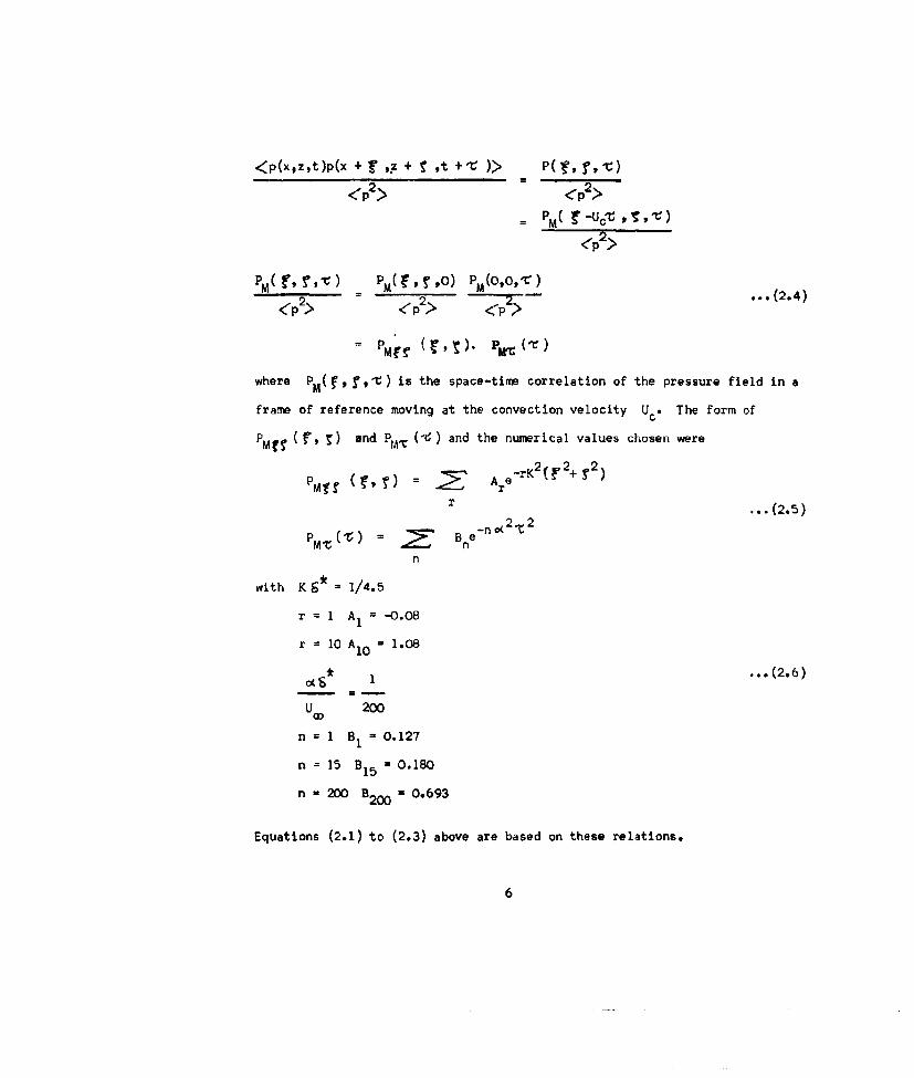
<p(x,z,t)p(x + " 9x + T ,t +,r )> P(,f, r',V)<P2 >P2>

<,p2 >

<p2> <_p2> < .. (.4

where PM( t r, ) is the space-time correlation of the pressure field in a

frame of reference moving at the convection velocity Uc* The form of

PM• ( M ' f ) and P,, (Is) and the numerical values chosen were

PMjf A r -rK (2'l) erK ' 2)

r ... (2.5)

PMC (Zc) = e Be (2 2

n

with K 6 = 1/4.5

r 1 A, = -0.08

r 10 A = 1.08

* 1 ... (2.6)

U 200

n = I B1 = 0.127

n = 15 B15 = 0.180

n = 200 B2 0 0 = 0,693

Equations (2.1) to (2.3) above are based on these relations.

6

2.1.4 Space-Time Correlation of Filtered Pressure Signals

For calculations of the response of a structure to boundary layermode

excitation using the normal/approacN the space-time correlation of the

pressure field in a narrow frequency band embracing the particular normal

mode is required. In essence this information is contained in the overall

correlations of the field and can be obtained by transformation, but it can

also be measured directly. Measurements of correlation in frequency bands

were made first by Harrison (4) but these results seemed to indicate a unique

dependence of the correlation on W 9/Uc. Such a relation leads to scale

anomalies at low frequencies. Additional measurements were made in the 6" x 2•"

wind tunnel(1) and the form of the results to be expected in the case of ?

slowly decaying pressure field as encountered in a slowly growing boundary

layer was also investigated(3).

It was concluded in Reference 3 that

(1) the frequency band space-time correlation in the flow direction

is periodic in time delay and spatial separation, undamped in time, but

with spatial damping depending on spatial separation and convection velocity.

(2) the variation in correlation amplitude with spatial separation

in the stream direction can be derived directly from the moving frame

overall autocorrelation of the pressure field.

A variation of this form removes the scale anomaly at low frequencies

and on the basis of the relations given in Equations (2.5) and (2.6) it was

found that the correlation amplitude could be expected to fall from unity to

0.2 with spatial separating increasing from zero to about 36 Sf, The derived

rate of spatial decay was found to be a tolerable representation of the

measured frequency band correlations (Fig. 7 of Reference 3) at least for

frequencies in the energy contained range of the spectrum.

7

2.2 Wall Pressure Fluctuations in the Laminar-Turbulent Transition Region

2.2.1 Aim of Experiments

The aim of these experiments is to continue the studies on the basic

mechanism of boundary layer turbulence by investigating the properties of the

turbulent processes found in the laminar-turbulent transition region, with

particular reference to wall pressure fluctuations.

The transition region has been selected for study since it is here

that the generation of turbulence first occurs in a field with known properties,

namely, the laminar boundary layer. It is hoped, therefore, that some insight

will be gained into the orocess of turbulence production, and hence ultimately,

the mechanism by which the turbulent boundary layer is sustained.

To make these studies use is being made of a hot-wire/microphone

combination. Selection of only those parts of the flow it is desired to study

will be made by another hot-wire driving a specially designed piece of apparatus

(see below). In this way, examination of turbulent spots at all stages of

their development may be made.

There have been some delays in this proqramme due to the difficulty of

setting up the instrumented transition region, and to the design and construction

of the special equipment needed to study intermittent phenomena. These

difficulties have been surmounteC, and some preliminary results are presented.

2.2.2 Experimental Programme

As it is now understood, the process of transition from laminar to

turbulent flow occurs gradually over a distance in the downstream direction

due to the superposition of distinct turbulent patches or spots. These

turbulent spots are believed to arise from the growth of small disturbances

in the laminar boundary layer which at some crucial stage in their development

form into a limited region of turbulence. This spot diffuses as it is

8

convected downstream by the mean flow until is loses its separate existence

through its interaction with other spots.

Over this region, where both laminar and turbulent flow regimes are

to be found, the degree of "spottiness" is described by the Intermittency

of the flow. The intermittency may be defined either is the fraction of time

for which the flow is laminar (the "laminar intermittency", denoted here by

G), or the fraction of time for which the flow is turbulent (the "turbulent

intermittency", denoted by Y ), As the latter is the one in general use in

the literature, the term intermittency will hereafter be used for turbulent

intermittency.

It is intended to study the turbulence in the spots in the transition

region. In particular, it is hoped to study the pressure fluctuations

associated with the transition region, the character of the turbulence in

the spots, and the position in the layer where the turbulence ip ears first.

This last aspect may be of importance in relition to the observed convection

of the pressure field of a turbulent layer it 0.3 of the free stream

velocity, since it has been suggested that this effect is due to phenomena

near the surface excited in conditions in the outer part of the boundary 1ý,yer.

Recent advances in knowledge of transition hive been made by

Schubauer, Klebanoff and others(5) using a vibrating ribbon to artificially

induce transition. It is not planned at the moment to use this technique,

but to study the statistical characteristics of the flow with natural

transition.

The basic configuration for the instrumentation is shown in Fig. 11.

Studies of the field will be made using a microphone and hot-wire (marked

"active wire"), acid the outputs from each will be analyzed both separately

and also as a joint record by correlation techniques. In order that

9

the turbulence in the region of the microphone may be limited to newly

developed spots, another hot-wire placed upstream of the microphono (marked

"monitor wire" will be used to operate a device which will shut off the

microphone signal if the turbulence is passing over the monitor wire. Although

only one channel is treated in this way, the effect after correlation is

as though both active hot-wire and microphone outputs were processed by the

monitor wire.

2.2.3 Instrumentation of the Transition Region

In order to make a study of the transition region with acoustic

instrumentation it is necessary to have some control over the position at which

transition occurs, since the exact position is very sensitive to external

flow conditions which vary from day to day, and it is not in general oossible

to move the microphones about readily. Basically, in a wind tunnel, the option

is between a boundary layer on a surface specially mounted for that purpose,

or using the tunnel wall.

At the time these measurements were first envisaged, the only low

noise tunnel immediately available was an induced flow one with a working

section measuring 6" x 2.5" which had been in use for turbulent boundary

layer measurements. The speed in the working section of this tunnel was fixed

at about 500 f.p.s. by a downstream sonic choke. As the flow had been

stabilized by placing boundary layer trips at the entrance it was not possible

to study transition on the working section walls, and so a plate was mounted

in the working section for this purpose. The high frequencies characteristic

of the flow, and the very limited space available, made the use of the piezo-

electric crystal transducers previously used in this tunnel for pressure

measurements imperative. It was not possible in the space to incorporate

any form of mechanical vibration isolation for the crystal, so a vibration

10

cancelling technique was evolved using two crystals. The two crystals were

mounted rigidly on the plate and one of them was screened from the pressure

field; their electrical outputs were combined to cancel the acceleration

effects. Unfortunately, the presence of the plate excited strong acoustic

resonances in the tunnel, and as it would have required extensive modification

to the tunnel to avoid them this arrangement was abandoned. The method of

vibration compensation of the pressure transducers is of some interest, however,

and the degree of success can be Judged from Fig. 1, where the suppression

of the plate modes is evident.

At this stage a new tunnel of a similar type to the one mentioned

above, but with a working section measuring 9" x 6", was complete. It w-s

thought that a suitable transition region could be established on the wall

of this tunnel at the beginning of the working section, the position of

transition being controlled by sucking away various amounts of the boundary

layer. However, the flow tended to become turbulent upstream of the suction

slots, so that satisfactory control of transition could not be obtained. It

was not considered feasible with the conditions present to re-stabilize the

boundary layer once it had become turbulent.

It was decided, therefore, to revert to study of the transition region

on a flat plate, and to adapt a low soeed tunnel specially for the work,

replacing the existing entrance with a new inlet, working section and

diffuser, and altering the fan gearing. The existing aluminium sheet dlffuser

was treated with "Aquaplas", and as much of the new structure as possible

was made with acoustically inert fibre board. The resulting tunnel offers

a speed of up to 100 fop.s, In the working section. A diagram of the

arrangement is shown in Fig. 2, and of the working section in Fig. 3.

The working surface is a f" brass plate, highly polished, with a flat

11

upper surface and a 60 wedge cut on the leading edge. A slight waviness

is visible to the eye, but the surface is smooth to the touch. A small

hole, diameter 0.030", is drilled 7" from the leading edge, giving access to

a cavity for a *0 condenser microphone (Brdel and Kjaer type 4134) which is

mounted on the underside of the plate, and recessed to within 0.029' of

the top surface. Control of boundary layer transition is affected by

adjusting the pressure gradient in the working section by means of flexible

wall liners.

2.2.4 Turbdlence Monitoring and Gating Equipment

Fundamental to the concept of these experiments is the ability of the

instrumentation to distinguish between signals characteristic of laminar and

turbulent flow. The way in which the apparatus for doing this function is

described below.

The core of this apparatus is a detecting (or rectifying) system to

which a variable bias may be applied. To illustrate the working, suppose

for simplicity that the signal to be examined is a sine wave, as shown in

Fig. 4 and we wish to know for what fraction of the Period T the amplitude

is above some arbitrary level, y. It will be seen that at time tI the

amplitude becomes greater than y, and stays so until time t 2 ; the appropriate

fraction is

G = (t - t1 )/r ...(2.7)

since tI = sinl y

t2 a 11" - sinl y

The output of an ideal device for a given setting, y, would be given

12

by Equation 2.7, and varies from G = 0 (level never above y for y > 1) to

G = 0.5 (half wave rectification) for y = 0, when the apparatus is examining

positive parts of the signal. In practice it is necessary that an increasing

(decreasing) signal exceed (fall below) the setting y by some small amount

before the apparatus can be made aware of it. Errors introduced by this

effect are grý?atest at the peak. This and other similar effects due to

finite operating times can, however, be reduced by careful design. Some

idea of the magnitude of possible errors can be obtained from Table 1.

TABLE 1

Error due to Non-Ideal Operation of Trigger Circuit

for Positive Going Portion of Sine Waves

Necessary excess in/, 0.2 0.4 0.6 0.8 0.95

fraction of signal -" 0

0.01 0.003 0.004 0.005 0.009 0.018

0.05 0.007 0.008 0.010 0.018 0.035

0.10 0.033 0.038 0.049 0.088 0.175

Error given in fraction of whole period.

If this basic device is presented with an intermittent signal •nd

the level y made just high enough not to be reached by the instrument

noise (see Fig. 6), then the device will "fire" at the peaks, but there will

be a dead zone around the axis, equal tn 2y, in which it will shut off. To

overcome this, it is necessary to build in a "memory" which holds the device

on for long enough to ensure that there is no further critical peak to follow.

The last super-critical peak will be followed then by a fallacious extension

13

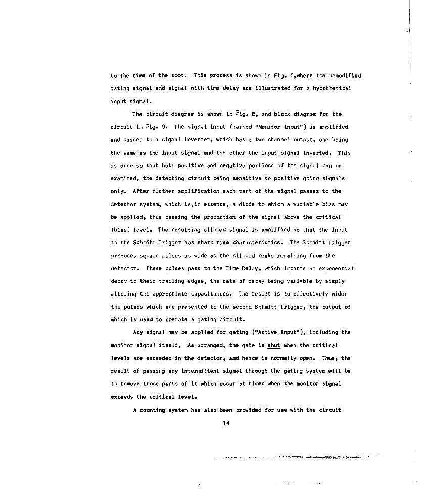
to the time of the spot. This process is shown in Fig. 6,where the unmodified

gating signal and signal with time delay are illustrated for a hypothetical

input signal.

The circuit diagram is shown in Fig. 8, and block diagram for the

circuit in Fig. 9. The signal input (marked "Monitor input") is amplified

and passes to a signal inverter, which has a two-channel outout, one being

the same as the input signal and the other the input signal inverted. This

is done so that both positive and negative portions of the signal can be

examined, the detecting circuit being sensitive to positive going signals

only. After further amplification each part of the signal passes to the

detector system, which is,in essence, a diode to which a variable bias may

be applied, thus passing the proportion of the signal above the critical

(bias) level. The resulting clipped signal is amplified so that the input

to the Schmitt Trigger has sharp rise characteristics. The Schmitt Trigger

produces square pulses as wide as the clipped peaks remaining from the

detector. These pulses pass to the Time Delay, which imparts an exponential

decay to their trailing edges, the rate of decay being variqble by simply

altering the appropriate capacitances. The result is to effectively widen

the pulses which are presented to the second Schmitt Trigger, the output of

which is used to operate a gating circuit.

Any signal may be applied for gating ("Active input"), including the

monitor signal itself. As arranged, the gate is shut when the critical

levels are exceeded in the detector, and hence is normally open. Thus, the

result of passing any intermittent signal through the gating system will be

to remove those parts of it which occur at times when the monitor signal

exceeds the critical level.

A counting system has also been provided for use with the circuit

14

2

for quantitative measurements of intermittency. In this case, the input to

the gate is a 200 kcps sine wave. The output is passed through three

binary counters, which reduce the effective frequency to 12.5 kcps, before

operating a timed decade counter. In this way the fraction of the time for

which the monitor signal is sub-critical is simply the ratio of the counts

with and without monitor input.

The last mentioned facility provides an accurate means of assessing

the accuracy of the device, since by varying the clip level in the detector

it is possible to determine how much cf the given signal is greater than a

given amplitude - effectively a probability analyser. Thus for a sine wave,

the fraction is given by Equation 2.7, while a similar evaluation may be made

for white noise. The results of actual tests are shown In Figs. 5 and 7. It is

seen that the operation of the equipment is satisfactory.

2.2.5 Results Obtained to Date

As this equipment was only made operational a short time before this

writing it has not been possible to accumulate any extensive experimental

results. However, some preliminary results nave been taken, and are

presented below.

2.2.5.1 Calibration

The initial calibration of the microphone showed a flat response

to about 2000 c.p.s. after which acoustic resonances produced a rather peaky

and generally rising response to about 10,000 c.p.s. The application of

damping material in the form of steel wool in the probe bore has reduced the

peaks, although the gradual rise is still present. All the same the response

curve is flat to within t 4 db up to 10 kcps., which is above the expected

cut-off frequency for the spectrum of the turbulence given by the Strouhal

number relation

15

f 0*/UooeO. 1

leading to f-6000 c.p.s. for U = 100 f.p.s.

e = 0.020"

The background noise, which is dominated by discrete fan frequencies

at about 150 c.p.s. and (to a lesser extent) at 300 c.p.s., is Pt in

acceptable level of about 94 db, although the low frequencies do show up in

the cerrelation coefficient obtained from hot-wire and microphone signals,

and will be eliminated by filtering when necessary. The free stream turbulence

level, as measured with the new low-noise transistor hot-wire gear, is about

0.23 of the free stream mean velocity, and as this level does not seem to be

having any adverse effect on the transition phenomenon, no attempt is being

made to reduce it at present.

To-examine different parts of the transition region, it is necessary

to alter the pressure gradient slightly with the tunnel liners. While this gives

the microphone effectively a variable x co-ordinate relative to the beginning

of the transition region, it also has some effect on the length of the actual

zone over which transition occurs. An estimate of the extent of the transition

region is to be had if it is assumed that the plot of intermittency v. distance

along the plate resembles an integrated Gaussian Er.Lor function. There is

experimental support for this assumption. The intermittency measured at

two points 4.2" apart was 0.138 and 0.778. For this case turbulence can be

expected for 1% of the time 4.5" upstream of the leading station, and 90% at 3.5"

downstream of the trailing station, although the assumption of Gaussian form

is almost certainly in error at this distance. However, the extent of the

region I.s probably of the order of about 9".

16

2.2.5.2 Intermittency Measurements

Fig. 12 shows intermittency measured at various stbtions in the boundary

layer ;or two stations in the transition region, one where the layer is mainly

laminar and the other where the layer is mainly turbulent. Though it is

inevitable with such measurements that there should be rel'tively large

scatter, both curves are quite well defined. It will be seen that there

exists a marked variation in the measured intermittency across the boundary

layer, maximum values being observed at about 0.15 S and 0.65 S , where 9 is

the thickness of the undisturbed laminar layer. If one oart of the layer

predominates in the production of turbulent spots, and it is assumed that

the spots grow uniformly as they are convected downstream, it may be shown

that the observed intermittency in this region will be higher than elsewhere.

It is possible, therefore, that one or both of the maxima observed In Fig. 12

correspond to areas of turbulence production.

2.2.5.3 Pressure Measurements

Measurements havE also been made of the pressure fluctuations, using

a hot-wire placed immediately over the microphone to evaluate the intermiltency.

The hot-wire signal is to be pr'ferred for this ourr,ose to the microphone

output as the signal/noise ratio is much better, but it has the disadvantage

that (as can be seen from Fig. 12 ) the intermittency measured -t a fixed

distance from the surface will only approximately represent the value of tho

wall pressure intermittency; the value obtained in this way, however, can he

expected to be fairly representative of the pressure intermittency. The

microphone output was integrated over a period of 30 seconds and divided by

this intermittency to arrive at a value for the r.m.s. wall nressure

associated with the turbulent spots.

Measurements with full turbulence at a flow speed of 70 feet per

17

second gave a pressure level of 104 db re 0.0002 dyne/cm . For this measure-

ment the microphone was calibrated against a standard noise source. This

makes the ratio

p'/q = 9.5 x 10"3

where p' is the r.m.s. value of the pressure fluctuations, and q is the

(4)dynamic pressure, which is the same as that obtained by Harrison This

preliminary figure is subject to revision, but indicates no significant difference

from the fully developed turbulent boundary layer.

The pressure associated with the spots for different intermittencies

(different effective downstream stations) is shown in Fig. 10, together with

the accuracy limits. As the intermittency approachcs zero, (fully laminar),

both the integrated value of the pressure signal and the divisor ( d ) become

very small. If the error in the r.m.s. pressure P is p, and in the measured

intermittency Y is g, then the quotient is

pg - P-Ftp~pt =

-..g

Since approximately '= kP

then P lI kP/y P (g+kp

it q/Y 1( 7

p and g are fixed in any given situation so that the limit lines vary

hyperbolically with Y . The limits are given for 2 error in P, -nd 3 in

Y . Both are rather optimistic estimates, but it is seen that the resulting

lines nearly enclose the pressure points from fully turbulent down to about

3We turbulent. Agreement is poorer at very low values where the error is

of the order of the mean value. The mean value used in Fig. 10 may be made

to coincide with the fully turbulent value ( ' 1.0) by using a different

value of intermittency; as discussed in Section 2.2.5.2 above, the precise18

intermittency which is applicable is still in doubt. Fig. 11 then indicates

that the pressure field associated with the turbulent spots is similar to

that of fully developed turbulence.

2.2.5.4 Continuation

Work is proceeding for the time being with the single wire and

microphone combination discussed above. In particular, further work is

being done on the variation of intermittency across the boundary layer, and

on the variation of amplitude distribution, which has been observed to be

markedly skew. It is proposed not to proceed with two wire work until the

possibilities of the present configuration have been exploited; the

necessary facilities for doing this are already available.

3. Theoretical Response of Panel to Turbulent Bouneary Layer Excitation

3.1 Results to Date

The work done so far has been based on the results derived by Powell(6)

for the response of structures to random excitations, and solutions are,

therefore, obtained as the sum of solutions in each of a multitude of normal

modes. The limitation of this approach is that response in each mode hAs

to be derived separately, with the consequence that, in general, a largeamount

of computation is needed to get even an approximate evaluation of the panel

displacements in quite a narrow frequency range.

As yet the range of frequencies covered is limited to the region

0 - 1000 c/s. which includes the first 15 panel modes.

19

3.2 Basis- of Calculitions

2.21 Equations used

Equation (13a) of Reference 6 for the power spectral density of panel

displacement can be written in tho form

(f) 2rr(f)

+ rr(R)*s(R) A j2 Nrs,(f) ... (3.1)+: z,r s IYrII SI

where 3"2 (f) 1 AI A A P (f(s,s'1_ )r(s) Ls c _')d 2 s d 2 s'

p

S -- h•,11) , d's d's'AI . A... (3.2)

I fA 2(r2s) d 2s ; A : Panel Area ... (3.3)

Here I Z(f), I p(f) are power spectral densities of panel displacement

z at R, and exciting pressurc p respectively, at a frequency f c/s.

Sp(f;s,_s'; -r) is the cross-Power spectral density of the exritAtion,

r(s) is the mode shape considered evaluated at point s.

Pf(•,(,r ) -- , is normalised cross-power spectral density

of the excitation

- 2rf

Y Yre eir is panel impedance for mode r.

20

3.2.2 Panel Impedance

The form used here is

SYrI = Mr • 2 W • 2 2 + ý2 Wr4ý . I22 :If, 2

= M L O + 1 A

r r W

tan- O ... (3.5)

ar

Here A, a "hysteretic" damping coefficient, is taken as 0.005, but the

actual value taken has little significance, except for frequencies near to

the natural frequency for the mode considered, provided only thit it is of

the right order of magnitude.

3.2.3 Effect of Cross Terms

As stated in the Section 3.1 we are confining our activities for the

moment to the low frequency range, so that it seems to be justifiable to

assume that

-= 'r -s

will not be too close to zero, and, hence, that Pf( , f • ) ill be

appreciably less than Pf( , ,0). This fact, co'.b-ned 'ith the fact that

the int-gral of a ?oroduct of modal. functions over part of the p'nel area

will usually be less than the integral of the square of either of the modal

functions over the same area, leads us to assume that

2Nrs (f)• < 2Nrr(f) ... (36)

r~s

The validity or this assumption for the particular correlation

21

function assumed is one of the matters that is to be investigated later.

Equation (3.1) is thus used in the reduced form

It,(f) R) •r AI J2Nrr(f) ... (3.7)

IMp_(f) (Yr 1 2

3.3 Correlation Function

3.3.1 General Form

In Reference 3 the following form for Pf( ,j -r) for a slowly

decaying pressure pattern is derived:

NRUc, O) c c

where P M-(r) is the autocorrelation function referred to axes moving with

Mcc

convection velocity Uc, whilst the term

is taken to be the same as the ov(erall lateral space correlation PMIS (01,

So (3.8) is taken as

Pf( ,1P Mjr (0,; PMC- U Cosuk - -) *...(3.9)

(See Reference 3, Section 4 from which this is taken).

i.e. P = PLAT X PLOW .... (3.10)

PLAT' PL0N3 are overall lateral space correlation and longitudinal space

correlation in required narrow frequency bands respectively.

22

3.3.2 Assumed Form for Boundary Layr Tunnel Correlation Function

Because of its analytical simplicity, the forin which has been assumed

initially for PMC (V ) is that taken by Dyer in Reference 7. However, the

computer programme can be extended to include correlation functions such as

that proposed in Reference 2.

p MC(-,9) -- e..3.1

where aUOD = 30

Here Uo0 = 500 ft/sec

= 0.1"

so that 9 = 0.5 m.sec.

Thus we can take

p LONG3 PNIV~' Cos "c c

2x cos 2+.-~

so = separation in longitudinal direction for first zero of PLOW)

L = log decrement based on first (negative) ?eak.

i.e. for = 21.

Then 29 f t 2%t k A

0= 00 ft....(3.13)f

= 1200 ins.f

23

L_ A

0= 2 ... (3.14)

f

There is very little experimental information on the value of PLAT' It will

be assumed that

a = 2.5 • * 0.25 ins ... (3.15)

and the maximum negative value is 0.05.

So we take

PLAT = exp TL t I cos 2111 -L ... (3.16)

where 3.0 ... (3.17)

Equations (3.12) - (3.17) inclusive substituted into (3.10) jive the assumed

fcrrn ,For the correlation function.

3.3.3 Assumed Form for the Lorrelation Function for the Siren Tunnel

Here we assume PLAT : 1 ... (3.18)

(Reference 8 Figure 14),

and assuming that for a given frequency the effective part of the pressure

field is a cosine wave propagatingj at the s~eed of sound, we get

SL = 0 ... (3.19)

o 3300 ins. ... (3.20)f

so that

, o) = PLOW

with volues given in Equations (3.19) and (3.20).

24

3.4 Evaluation of j- rr(f)

In Reference 9 a relationship is derived for J2Nrr(f) as defined in

Equation (3.2)*, for a correlation function of the form

~V -a Lill -&T 15Pf(eLo) = e cos bLs ... (3.22)

with ,r(j) taking the form

_t'r (-) " )(s) = sin mx sin nwy ... (3.23)

L Lx y

The mode shape assumed here is appropriate to having the panel edges simply

supported but there are indications that the effect of the plate boundary

conditions on the integrated value of j 2Nrr(f) is small for the fundamental

mode, and gets progressively smaller as the order of the mode increases, so

that the error introduced by the assumption is probably small.

Using relations similar to Equations (3.22) and (3.23), Reference

9 derives

J2 (f ) 160LT.(mnv•)2 ... (3.24)

where

= j p [ I -(-l)m e cos bL + 4q(-1)m eaL sin bL

2 111. ... (3(25)mr2+ - -4.-- ... (3.26)

*This definition, rather than that used by Powell, is used to el minate theeffects of any arbitrary coefficients arising in the choice of rL).

25

S(b 1212 2 2(bLU 2= 11+1 - -(~2 (4 --) ... (3.27)

S= (X ,tl÷ v; (-...(3.27)

= t + 1+(... (3.29)

where all symbols except numerical constants are understood to have suffix

and where o = L, T.

mL = m, mr = n.

The correspondence between Equation (3.22) and Equation (3.12) and (3.16)

is given by

aL i , * ... (3.31)

21 , 2 o3.5 Evaluation of .IYr12

3.5.1

From Equation (3.5)

l¥I 2 = r2 41[1 - J+,, ... (3.32)

where r= A mr2C) dL s = m, ... (3.33)

mn mass/unit area of panel.

Thus the evaluation of Iyrl 2 cenires on the evaluation of the natural

frequencies of the panel in each of the modes considered.

26

3.5.2 Evaluation of

r

The natural frequency of the panel is derived using the work reported

in Reference 10. The actual boundary conditions (i.e. fixed or supported

depending on the panel) are used here, as distinct from the assumption made

for Equation (3.23).

3.6 Final Equation

We now have all that is required for the evaluation ofbz (f) since

for Equation (3.8)

mzn (f) * 1n 2 +(A 2N) . 3

where 2 (S d2s ... (3.35)

and the >n1 (s), W M are those dictated by the actual plate boundary condition.

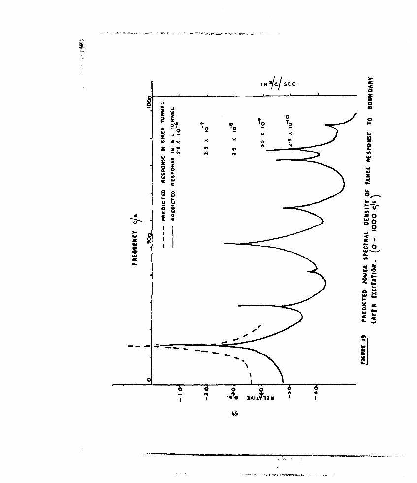
3.7 Panel Results

The panel being evaluated at the moment is an 0.005" thick steel

panel, 3.5" square, and the panel is fastened to a soltd member in such a

way that it is reasonable to take it as having fully fixed edges.

The process indicated above has been carried through for this oanel,

the lowest 15 modes having been considered for the response in the boundary

layer tunnel, but only, so far, the lowest mode for the siren tunnel

case&

The results of the computations are shown in Fig. 13.

27

4. Response of Panels to Boundary Layer Excitation (Experimental)

4.1

The study of structural response to turbulent boundary layer excitation

is of interest in relation to two major engineering problems; one is the

problem of noise in and around aircraft and submarines where a major

contribution results from the actioa of the structure as a transducer in

converting the hydrodynamic pressures in the boundary layer into acoustic

pressures and the other is that prolonged excitation by the boundary layer

may cause structural failure due to fatigue. In an investigation into

either of these problems it is desirable to have a knowledge of the response

of simpler elements of a structure, such as panels, to random excitation.

Panel response to boundary layer excitation has been studied

theoretically by several authors using either panel normal modes or the

concept of coincidence (i.e. frequency and wavelength matching between

exciting force and panel response). However, up to date there has been

little or no experimental verification of the accuracy of estimation provided

by either of these approaches and hence it is the object of the current

investigation to obtain data, by measuring the response of panels to boundary

layer excitation in air, which might provide (a) justification for the

calculation procedures and (b) a clearer insight into the mechanism of the

response of a structure to this type of excitation. The problem is complex

and the model structures studied initially must of necessity be simple in

form so that they are amenable to calculation. For this reason the

measurements are being made on panels of square or rectangular plan-form,

having fixed edges and having no longitudinal or transverse stiffeners.

In order to interpret the measurements fully, the vibrational

28

characteristics of the specimens must be known. For this reason the

frequencies and shapes of the normal modes of the panels are determined

experimentally using discrete frequency excitation. To complete the

investigation, the response of the panels under test is being calculated

theoretically, as described in Section (3) above, for comparison with the

experimental values.

4.2 Preliminary Measurements in the 6" x 24-" Wind Tunnel

The initial work on panel response to boundary layer noise excitation

was carried out in the supersonic working section of the 6" x 2ý-" tunnel.

It was intended to investigate possible coincidence effects at supersonic

convection velocities of the boundary layer pressure field, with particular

reference to the generation of Mach waves by supersonic flexural ripples in

the panel. This study proved impracticable in this small scale flow and

when Mr. D.J.M. Williams left the group, this work was discontinued in

favour of the panel displacement measurements in the 9" x 6" tunnel.

The work did, howver, highlight one of the major difficulties in

these investigations, namely the construction of the panel. When using thin

sheets of metal it is extremely difficult to obtain a panel which is flat

and yet under zero or negligible tension. The panel was formed from a sheet

of brass, O.C05" thick, attached to a 6" diameter plug, the shape of the

vibrating panel being determined by a 31" square hole cut through the centre

of the plug. The first panel was stuck to the plug with epoxy resin but

the adhesive failed during trial runs in the tunnel. Later panels were

attached to the plug by clamping strips parallel to the edges of the square

hole. This method presented difficulties in fixing the brass sheet at the

corners of the cut-out ard introduced unknown and probably non-uniform

29

tension in the panel.

4.3 Test in the 9" x 6" Wind Tunnel

The measurements in the 9" x 6" tunnel are concerned with the dis-

placements of panels subjected to boundary layer excitation and hence are

of a rather different nature to those discussed above. The panels being

tested are similar to those used in the 6" x 2-2" tunnel in that they are

formed from a thin sheet of metal attached to a 6" diameter plug with the

hole in the plug again determining the shape of the vibrating region. The

panels currently being used are 3a-" square and either 0.005" or 0.010" thick.

The material used has, however, been changed frcm brass to steel, so that

the panels can be excited magnetically for deteirnination of their normal

modes of vibration.

Because of the possibility of introducing unknown tensions in thepanels, and hence creating unpredictable effects in their response (6) the

clamping procedure adopted in the earlier tests was not continued. Instead,

recourse was had to epoxy resins for bonding the steel sheets to the plugs.

It was found that, with care, the adhesives could withstand the static

pressure differentials imposed on them when placed in the wind-tunnel wall.

To obtain a good bond the surfaces are completely degreased by immersion in

a l1C solution of sodium metasilicate for a period of 10 minutes. The

brightness of the surfaces is then enhanced by immersing in an 85% phosphoric

d.id solution for 2 minutes.

dhilst the epoxy resin is setting, the plug and steel sheet are held

together in a jig so that the panel remains flat. This clamping, which

was not used when assembling the first 0.005" panel, does not cause panel

tensioning and the jig is removed when the resin hrs hardened. To avoid

30

differential thermal expansion between the plug and panel due to localised

heating, the resin is cured under normal room temperature. This does

however have the disadvantage of increasing the curing time anc slightly

decreasing the strength of the bond.

The construction of a typical Panel is shown in Fig. 14. The two

clamping strips, along sections of the plug peciweter, are positioned ifter

the resin has set and hence do not tension the panel. Their purpose is purely

precautionary and is to prevent the panel from being carried into the tunnel

in the event of a failure of the adhesive during tunnel operation. The

region around the clamping strips is built-up with resin to oresent n surface

which is flush with the tunnel wall.

4.4 Normal Modes

The normal modes of the panels are determined from panel response to

discrete frequency excitation. The natural frocuencies are obtained from

measurements of amplitude and phase (relative to the exciting forue) of the

panel vibrations and the mode shapes are observed visually when sand particles

are spread over the ?anel surface.

The frequencies of the low order modes were investigated, using

electromagnetic excitation, for the 0.005" panel made first. The values

obtained were found to be considerably higher thar. those estimated

theoretically (Status Report No. 8). In particular, the measured funda-

mental frequency was in the range 160 c.p.s. to 260 c.n.s. (subject to

positioning of equipment as discussed belcw) whilst the calculated value •as

141 c.p.s.

It Is believed that the discrepancy is due to the fact that the r.non],

when assembled, is not flat but has an appreciable curvature. This bow is

very difficult to control but a satisfactory degree of flatness can probably31

be achieved by the modified method of construction described in Section 4.3.

Some approximate calculations based on comparisons between the natural

freqoencies of spherical caps as derived by Reissner in Reference 11

and those for flat circular plates (Reference 12) indicate that the degree

of bowing to be expected can have an effect on the panel of similar magnitude

to that measured above. As the natural frequencies of flat square plates

of side a, and frat circular plates of diameter a differ by less than

3%, it is reasonable here to take the results for circular plates and apply

them directly to square ones.

Closer examination of the measurements showed that the "apparent

natural frequencies" depended markedly on the relative positions of the

exciter, panel and proximity transducer used to measure the vibrations. This

was most critical when exciter and transducer were both at the panel centre

and, for these conditions, the observed variation of panel "fundamental"

frequen',y with distance of transducer from panel is shown in Fig. 15.

Unfortunately, oefore this phenomenon could be fully explored, the panel

was damaged and l1di to be replaced. The investigation will, however, continue

on the second :anel using electromajnetic and acoustic excitation - the

lattcr beirnj of use only for modes for which the generalised force is non-

zero.

4.5 Boundary Layer Excitation

Tiv panel is mounted in the side wall of the 9" x 6" induced flow

wind tunnel. The static pressure in the tunnel working section is oelow

atmosoheric and in the sub-sonic section the pressure differential is 2.3

to 2.4 p.s.i., dependong on position; this has a marked effect on the

vibration of the thin panels placed in the tunnel wall.

The displacement power spectrum for the first 0.005" panel under a

32

pressure differential of 2.34 p.s.i. was shown in Fig.2 of Status Report

No. 8. The main purpose of these measurements was, however, a comparison

of the amplitudes of the panel vibration and the background vibration of the

traverse gear and wind tunnel. It was found that the latter vibration was

at least 20 db below the former throughout the spectrum and would therefore

not influence measurements of panel vibration.

The outer face of the panel has now been enclosed by a sealed box in

which the static pressure can be reduced to that of the tunnel. The background

vibration is till of the same order of magnitude as previously measured but

the overall panel vibration amplitude has increased by a factor of about 4.

Panel displacement spectra have been measured at several positions on the

surface of a second 0.005" panel and results for three of these positions

are shown in Fig. 16. The pressure differential across the panel during the

vibration measurements was 0.003 p.s.i.

The spectra show the presence of several panel normal modes and are

in this respect considerably different in character from those previously

measured under a greater pressure differential. Fig. 16 ulearly shows the

variation of the relative magnitude of the response in each mode with

variation of position on the surface (i.e. as the vibration pick-up chinges

position in relation to the modes and antimodes of the mode), for example,

the peak at 790 c.p.s. (Fig. 16 (a)) is barely discernible in Fig. 16(b) but

has returned again in Fig. 16(c).

The natural frequencies of this panel have not yet been determined

experimiantally and hence the particular modes present in the above spectra

cannot yet be identified. The frequency of the predominant peak (20.5 c.p.s.)

does not however correspond with the calculated fundamental frequency

(141 c.p.s.) of the panel.

33

5. Sound Radiation from a Turbulent Boundary Layer on a Rigid Surface

On the basis of the correlation pattern given by Equations (2.4) to

(2.6) the acoustic power output from unit area of a (large) surface subject

to turbulent boundary layer flow was found to be given by(2)

6 3 = 2.10-4 ... (5.1)

34

REFERENCES

1. Bull, M.K. "Instrumentation for and PreliminaryMeasurements of Space-Time Correlationsand Convection Velocities of the-PressureField of a Turbulent Boundary Layer"University of Southampton ReportA.A.S.U. 149, August 1960.

2. Bull, M.K. "Some Results of Experimental InvestigationsWillis, J.L. of the surface Pressure Field due to a

Turbulent Boundary Layer"

University of Southampton ReportA.A.S.U. 199, November 1961.ASD-TDR-62-h25

3. Bull, M.K. "Space-Time Correlations of the Boundary LayerPressure Field in Narrow Frequency Bands"University of Southampton ReportA.A.S.U. 200, Decenber 1961.ASD-TDR-62-722

4. Harrison, M. "Pressure Fluctuations on the Wall Adjacentto a Turbulent Boundary Layer"David Taylor Model Basin Report 1260December 1958.

5. Klebanoff, P.S. "The bhree-Dimensional Nature of BounduryTidstrom, K.D. Layer Instability"Sargent, L.M. 31. Fl. Mechs. Vol.12 1962.

6. Powell, A. "On the Fatigue Failure of Structures dueto Vibrations Excited by Random PressureFields"J.A.S.A. 30, p.1130, 1958.

7. Dyer, I. "Sound Radiation into a Closed Space fromBoundary Layer Turbulence"B.B.N. Report 602

8. Clarkson, B.L. "The University of Southampton RandomPietrusewicz, S.A. Siren Facility"

University of Southampton ReportA.A.S.U. 204

9. Clarke, M.J. "Response of a Rectangular Panel toRandom Pressures"University of Southampton Report(to be published)

35

10. Warburton, G.B. "The Vibration of Rectangular Plates"Proc. I. Mech, E. 168, p.371, 1954.

ll. Reissner, F. "On Vibrations of Shallow Spherical Shells"Jour. App. Phys. 17, p.1038, December, 1948.

12. Morse, P.M. "Vibration and Sound"(Mc3raw Hill) p.210.

36

00

8'

' 0 O

0

o 10

00

z IIILI

con

(21vs iAMlaW) .ndJino W1IAVD

37______

InI

C4ul

La''

1L4L

0 C

U a

38

1-0 FICUBF 4

OPERATION OF MONITORINGEQUIPMENT ON SINE WAVE I

INPUT.T/2

-t2 TIME

1.0

0.9

t

0

o- F 1IGUREiCLIP OF SINE WAVE

t- POSITIVE GOING

"" NEGATIVE GOING

07 THE THEORETICAL RESULT

IS SHOWN BY THE

CONTINUOUS LINE

0.6

1.0 0,5 0-6 0,4 0.2 0

+ Y AND- -Y

39

+ CLI LEVE

RA TIME

i nriGATING PULSES TMWITHOUT TIME DE LAY

GATING PULSES TMWITH TIME DELAY

tit-URF A MONITORINC OlF INTERMITTOMTL TitElLFId7 --IGNALS

-0.

o -0 CLIP OF WHITE NOISE+ POSITIVE GOING

O 0.7 THE THEORETICAL RESULT IS SHOWN

z - by THE CONTINUOUS LINE

S1. I.6 14 1.2 90 O111 04 04 0.2 40ftw.?7. CLIP AT STrATD Nuborf or wrAI'mW Svilwous,

40

CFIAft.. WI

I -D

1.

Lk-

Sam

0* C

a IC

LL.

w ~ w

* ~;I

0 0Lz 4A z

a. 4-

TO NEXT

POINT

1,'50 ASSUMES UNCERTAINTY OF

* SeN DETERMINATION OF

t-6NDETERMINATIONOF I

40

z 1 - EN5AU

OPF MEASURED POINTS O

FULLY TURBULENT0.75. VALUE

0.5 Oil 0;2 0p 0 14 0;5 0,*6 07 0-8 0-9 I0

TURbULINT INTIRWMITNCY-

FIGIAF 10 BSPF~EFI~b IULN P1

43

ACTIV EMJONITOR X

X HOT WIREHOT WIRE

/ 7 /Z// 7/f///U7 L..jr 1777i///

M ICROPHE

FFGURE II. BASIC CONFIGURATION FOR MEASUREMENTS.

0

9 -40

0

0.z

30

-20

a 10

0 01 0 02 0"3 04 5 06 0"7 0Oi 0.9

INTERMITTENCY OR VELOCITY.

FICVUI 12. YARIATION OF INTEINITTENCY ACROSS SOUNIDY LAYER.

444

#I'I

IN2

/c SECII1

UZ -J

Zz 0z

't ToIi

w- - - x

a-

I t-

z=

-CZ

2o

UcU0

tj 0I- *- ~w

MAu

Sale

g dog

0 ,L

'20 B1,4o3

45a

in

-J

-ax Ofj

in a

z

4 us

K PC

0 'a2 0

ia~yK ao A~n~* ia.mLvvdv

47Z

't

cc

o 0

zz

0 o

t u 0 0A z

0

L4

UNCLASSIFIED

UNCLASSIFIED