Active Query Forwarding in Sensor Networks(ACQUIRE)

Narayanan Sadagopan†, Bhaskar Krishnamachari§†, Ahmed Helmy§† Department of Computer Science

§Department of Electrical Engineering - SystemsUniversity of Southern California

Los Angeles, California{narayans, bkrishna, helmy}@usc.edu

June 11, 2003

1

Abstract

While sensor networks are going to be deployed in diverse application specific con-texts, one unifying view is to treat them essentially as distributed databases. Thesimplest mechanism to obtain information from this kind of a database is to floodqueries for named data within the network and obtain the relevant responses fromsources. However, if the queries are a) complex, b) one-shot, and c) for replicateddata, this simple approach can be highly inefficient. In the context of energy-starvedsensor networks, alternative strategies need to be examined for such queries.

We propose a novel and efficient mechanism for obtaining information in sensornetworks which we refer to as ACQUIRE. The basic principle behind ACQUIRE is toconsider the query as an active entity that is forwarded through the network (eitherrandomly or in some directed manner) in search of the solution. ACQUIRE alsoincorporates a look-ahead parameter d in the following manner: intermediate nodesthat handle the active query use information from all nodes within d hops in orderto partially resolve the query. When the active query is fully resolved, a completedresponse is sent directly back to the querying node.

We take a mathematical modelling approach in this paper to calculate the energycosts associated with ACQUIRE. The models permit us to characterize analyticallythe impact of critical parameters, and compare the performance of ACQUIRE withrespect to other schemes such as flooding-based querying (FBQ) and expanding ringsearch (ERS), in terms of energy usage, response latency and storage requirements.We show that with optimal parameter settings, depending on the update frequency,ACQUIRE obtains order of magnitude reduction over FBQ and potentially 60 to 85%energy reduction over ERS (in highly dynamic environments and high query rates). Weshow that these energy savings are provided in trade for increased response latency.The mathematical analysis is validated through extensive simulations.

2

1 Introduction

Wireless sensor networks are envisioned to consist of large numbers of devices, each capableof some limited computation, communication and sensing, operating in an unattended mode.These networks are intended for a broad range of environmental sensing applications fromweather data-collection to vehicle tracking and habitat monitoring [2, 3, 4]. The key challengein these unattended networks is dealing with the limited energy resources on the nodes.

With a small set of independent sensors it is possible to collect all measurements from eachdevice to a central warehouse and perform data-processing centrally. However, with large-scale networks of energy-constrained sensors this is not a scalable approach. It has beenargued that it is best to view such sensor networks as distributed databases [9, 10, 11, 16].There may be a central querier/data sink (or a collection of queriers/sinks) which issuesqueries that the network can respond to. Due to energy constraints it is desirable for muchof the data processing to be done in-network. This has led to the concept of data-centricinformation routing, in which the queries and responses are for named data as opposed tothe end-to-end address-centric routing performed in traditional networks.

Depending on the applications, there are likely to be different kinds of queries in these sensornetworks. The types of queries can be categorized in many ways, for example:

• Continuous queries, which result in extended data flows (e.g. “Report the measuredtemperature for the next 7 days with a frequency of 1 measurement per hour”) versusOne-shot queries, which have a simple response (e.g. “Is the current temperaturehigher than 70 degrees?”)

• Aggregate queries, which require the aggregation of information from several sources(e.g. “Report the calculated average temperature of all nodes in region X”) versusNon-aggregate queries which can be responded to by a single node (e.g. “What is thetemperature measured by node x?”)

• Complex queries, which consist of several sub-queries that are combined by conjunc-tions or disjunctions in an arbitrary manner (e.g. “What are the values of the followingvariables: X, Y, Z?” or “What is the value of (X AND Y) OR (Z)” versus simple queries,which have no sub-queries (e.g. “What is the value of the variable X?”) 1

• Queries for replicated data, in which the response to a given query can be provided bymany nodes (e.g. “Has a target been observed anywhere in the area?”) and queries forunique data, in which the response to a given query can be provided only by one node.

Flooding-based query mechanisms such as the Directed Diffusion data-centric routing scheme[5] are well-suited for continuous, aggregate queries. This is because the cost of the initialflooding of the interest can be amortized over the duration of the continuous flow from

1We assume that each sub-query is a query for some variable tracked by the sensor network.

3

the source(s) to sink(s). However, keeping in mind the severe energy constraints in sensornetworks, a one-size-fits-all approach is unlikely to provide efficient solutions for other typesof queries.

In this paper we propose a new data-centric querying mechanism, ACtive QUery forwardingIn sensoR nEtworks (ACQUIRE). Figure 1 shows the different categories of queries and thekinds of queries in sensor networks that ACQUIRE is well-suited for: one-shot, complexqueries for replicated data. As a motivation for ACQUIRE, we describe two scenarios whichinvolve such queries:

• Bird Habitat Monitoring Scenario: Imagine a network of acoustic sensors deployedin a wildlife reserve. The processor associated with each node is capable of analyzingand identifying bird-calls. Assume each node stores any bird-calls heard previously.The task “obtain sample calls for the following birds in the reserve: Blue Jay, Nightin-gale, Cardinal, Warbler” is a good example of a complex (because information is beingrequested about four birds), one-shot (because each sub-query can be answered basedon stored and current data) query, and is for replicated data (since many nodes in thenetwork are expected to have information on such birds). Another example of a com-plex, one-shot query in this network might be “return 5 locations where a Warbler’scall has been recorded” (the request for each location is a sub-query).

• Micro-Climate Data Collection Scenario: Imagine a heterogeneous network con-sisting of temperature sensors, humidity sensors, wind sensors, rain sensors, vibrationsensors etc. monitoring the micro-climate in some deployed area. It is possible toput together a number of separate basic queries such as “Give one location where thetemperature is greater than 80 degrees?”, “Give one location where there is rain at themoment in the area?”, and “Give one location where the wind conditions are currentlygreater than 20 mph?” can be combined together into a single batched query. Thiscomplex query is one-shot (as it asks only for current data) and is also for replicateddata (since several nodes in the network may be able to answer the queries2).

The principle behind ACQUIRE is to inject an active query packet into the network thatfollows a random (possibly even pre-determined or guided) trajectory through the network.At each step, the node which receives the active query performs a triggered, on-demand,update to obtain information from all neighbors within a look-ahead of d hops. As thisactive query progresses through the network it gets progressively resolved into smaller andsmaller components until it is completely solved and is returned back to the querying nodeas a completed response.

While most prior work in this area has relied on simulations in order to test and validate data-querying techniques, we have taken here a mathematical modelling approach that allows us

2There is an implicit assumption that the sub-queries can all be resolved. In this example, it is assumedthat there are such locations. Without this assumption, it is not be possible to do anything more intelligentthan querying all nodes in the network.

4

Figure 1: A categorization of queries in sensor networks: the shaded boxes represent the querycategories for which the ACQUIRE mechanism is well-suited.

to derive analytical expressions for the energy costs associated with ACQUIRE and compareit with other mechanisms, and to study rigorously the impact of various parameters suchas the value of the look-ahead parameter and the ratio of update rate to query rate. Ourmathematical analysis is validated through simulations.

The rest of the paper is organized as follows: in section 2 we describe some of the relatedwork in the literature. We provide a basic description of the ACQUIRE mechanism in section3. In section 4 we develop our mathematical model for ACQUIRE and derive expressionsfor the energy cost involved as a function of the number of queried variables, the look-aheadparameter, and the ratio of the refresh rate to the query rate. We develop similar models andenergy cost expressions for two alternative mechanisms: flooding based queries (FBQ) andexpanding ring search (ERS) in section 5. We first examine the impact of critical parameterson the energy cost of ACQUIRE and then compare it to the alternative approaches in section6. Our analytical models are validated by simulations in section 7. The average responselatency incurred by ACQUIRE, ERS and FBQ is analytically modelled in section 8, whilethe caching storage requirements are discussed in section 9. We discuss these results anddescribe the future work suggested we are planning to undertake in section 10. Finally, wepresent our concluding comments in section 11.

2 Related Work

Bonnet, Gehrke, and Seshadri [10, 11] as well as Yao and Gehrke [16] present the COUGARapproach which treats sensor networks as distributed databases, with users tasking the net-work with declarative queries which are then converted by a front-end query processor intoan efficient query plan for in-network processing. Similarly Govindan, Hellerstein, Hong etal. also argue in [9] that sensor networks ought to be viewed primarily as virtual databases,with query optimization performed via data-centric routing mechanisms within the network.

5

The efficient in-network computation of aggregate responses to queries is the subject of thepaper by Madden, Szewcyk et al. [19]. The ACQUIRE mechanism we describe in this pa-per is compatible with this database perspective, and can viewed as a data-centric routingmechanism that provides superior query optimization for responding to particular kinds ofqueries: complex, one-shot queries for duplicated data.

Intanagonwiwat, Govindan, Estrin and Heidemann propose and study Directed Diffusion [5,6], a data-centric protocol that is particularly useful for responding to long-standing/continuousqueries. In Directed Diffusion, an interest for named data is first distributed through the net-work via flooding (although optimizations are possible for geographically localized queries),and the sources with relevant data respond with the appropriate information stream. Theimpact of aggregation in improving the energy costs of such data-centric protocols is exam-ined by Krishnamachari, Estrin and Wicker in [7].

Also related to our work are the Information Driven Sensor Querying (IDSQ) and Con-strained Anisotropic Diffusion Routing (CADR) mechanisms proposed by Chu, Haussekerand Zhao [14]. In IDSQ, the sensors are selectively queried about correlated informationbased on a criterion that combines information gain and communication cost, while CADRroutes a query to its optimal destination by following an information gain gradient throughthe sensor network.

One technique that is close in spirit to ACQUIRE is the rumor-routing mechanism proposedrecently by Braginsky and Estrin in [21]. Their approach is quite interesting - sourceswith events launch mobile agents which execute random walks in the network resultingin event-paths. The queries issued by the querier/sink, in a manner somewhat similar toACQUIRE, are also mobile agents that follow random walks. Whenever a query agentintersects with an event-path, it uses that information to efficiently route itself to the locationof the event. Rumor routing is a mechanism to lower the interest-flooding cost for DirectedDiffusion in situations where geographical information may not be available. Rumor routingis not, however, geared primarily towards complex one-shot queries for replicated data (asACQUIRE is) and does not incorporate any look-ahead/update parameters. Moreover, ifdata is replicated, there might be multiple sources, each of which might initiate a randomwalk in the rumour-routing case. In such cases, rumour-routing may not be energy-efficient.

Other data-centric routing protocols proposed for sensor networks include SPIN for datadissemination by Heinzelman, Kulik and Balakrishnan [17], and LEACH for data collectionby Heinzelman, Chandrakasan and Balakrishnan [18].

The recent work by Ratnasamy, Karp et al. [13] presents the geographic hash table techniquefor data-centric storage (DCS) in sensor networks. This approach is particularly useful forstoring information to deal with historic queries (i.e. queries for non-current data). Inestimating the cost of local storage the authors of [13] assume the use of flooding-basedqueries, to which we provide an alternative in this paper. It is also be possible to conceiveof using our ACQUIRE scheme in conjunction with any DCS techniques that result inreplication (e.g. for robustness reasons).

6

Our work also has some similarities to techniques proposed for searching in unstructuredpeer-to-peer (P2P) overlay networks on the Internet. In particular, [22] discusses the pos-sibility of launching k-random walks through the unstructured P2P network for discoveringrequired files/data. This differs from our work in three respects: one is that the cost-modelis different in the two scenarios - in P2P networks one is primarily concerned with minimiz-ing bandwidth usage and delay while we are primarily concerned with minimizing energyconsumption; the second is that we incorporate the look-ahead parameter and allow forcomplex queries, which, as we show in this paper, significantly improves the performance ofsuch a search; and finally, the trajectories followed by active queries in ACQUIRE need notnecessarily be random walks, they could be directed and deterministically selected.

Our ACQUIRE mechanism combines a trajectory for active queries with a localized updatemechanism whereby each node on the path utilizes information about all the nodes withina look-ahead of d hops. The size of this look-ahead parameter effects a tradeoff between theinformation obtained (which helps reduce the length of the overall trajectory) and the cost forobtaining the information. This look-ahead region is somewhat similar in spirit to the notionof zones in the Zone Routing Protocol (ZRP) [15] and to the notion of neighborhoods in theContact-based Architecture for Resource Discovery (CARD) [12] developed for mobile ad-hocnetworks. One key difference is that in ACQUIRE, only nodes on the active query trajectoryneed to have this look-ahead information and the neighborhood updates are triggered on-demand, if current information happens to be obsolete.

While the trajectory for the active queries is assumed to be random in our modelling inthis paper, it is possible to envision pre-determined trajectories as well. One interestingnew mechanism that we could combine ACQUIRE with is the idea of routing along curves,described by Nath and Niculescu in [20].

3 Basic Description of ACQUIRE

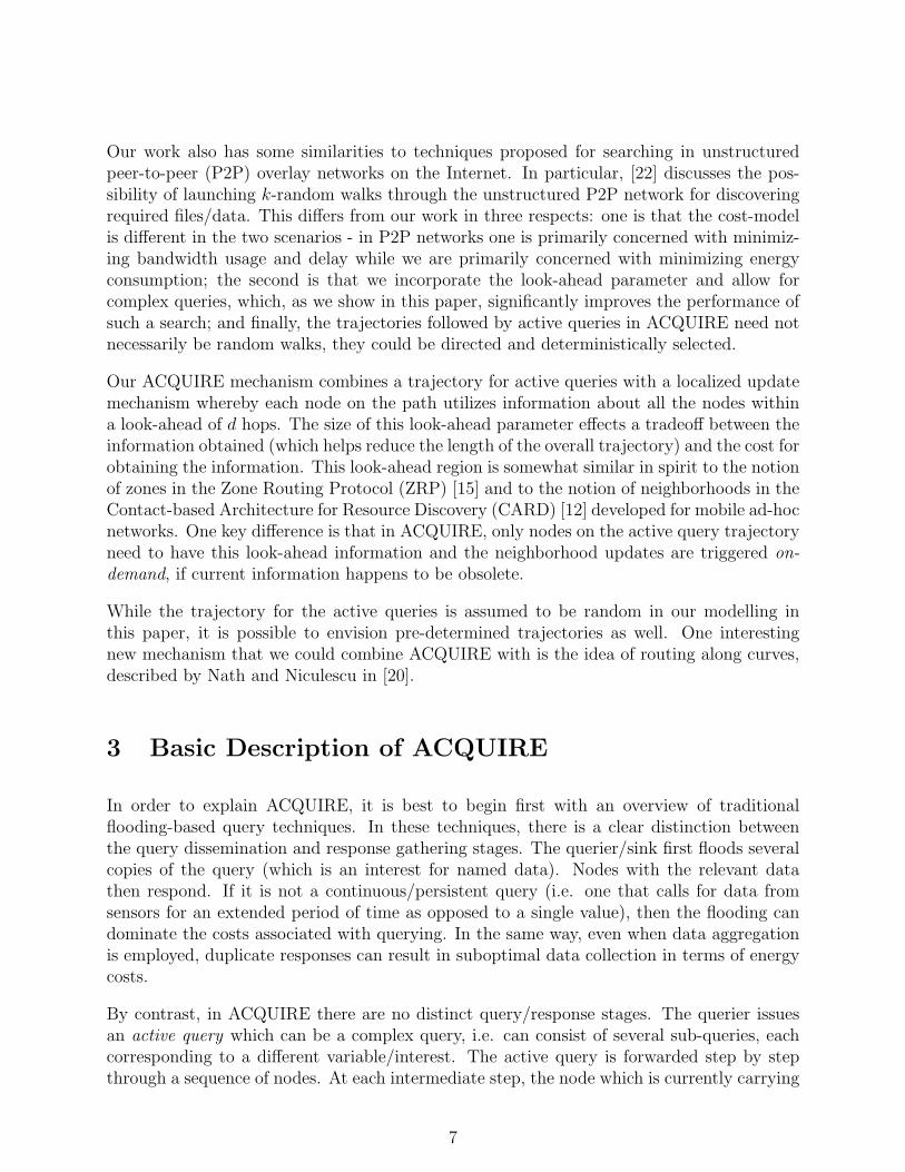
In order to explain ACQUIRE, it is best to begin first with an overview of traditionalflooding-based query techniques. In these techniques, there is a clear distinction betweenthe query dissemination and response gathering stages. The querier/sink first floods severalcopies of the query (which is an interest for named data). Nodes with the relevant datathen respond. If it is not a continuous/persistent query (i.e. one that calls for data fromsensors for an extended period of time as opposed to a single value), then the flooding candominate the costs associated with querying. In the same way, even when data aggregationis employed, duplicate responses can result in suboptimal data collection in terms of energycosts.

By contrast, in ACQUIRE there are no distinct query/response stages. The querier issuesan active query which can be a complex query, i.e. can consist of several sub-queries, eachcorresponding to a different variable/interest. The active query is forwarded step by stepthrough a sequence of nodes. At each intermediate step, the node which is currently carrying

7

the active query (the active node) utilizes updates received from all nodes within a lookaheadof d hops in order to resolve the query partially. New updates are triggered reactively bythe active node upon reception of the active query only if the current information it has isobsolete (i.e. if the last update occurred too long ago). After the active node has resolvedthe active query partially, i.e. after it has utilized its local knowledge to answer as muchof the complex query as possible, it chooses a next node to forward this active query to.This choice may be done in a random manner (i.e. the active query executes a randomwalk) or directed intelligently based on other information, for example in such a way as toguarantee the maximum possible further resolution of the query. Thus as the active queryproceeds through the network, it keeps getting “smaller” as pieces of it become resolved,until eventually it reaches an active node which is able to completely resolve the query,i.e. answer the last remaining piece of the original query. At this point, the active querybecomes a completed response and is routed back directly (along either the reverse path orthe shortest path) to the originating querier.

The difference between traditional querying techniques and ACQUIRE, and the lookaheadscheme of ACQUIRE are illustrated in figures 2 and 3 respectively.

4 Analysis of ACQUIRE

We now build a mathematical model to analyze the performance of ACQUIRE in terms of itsexpected completion time and associated energy costs. This will also enable us to determinethe optimal look-ahead parameter d. There are several metrics for energy costs. In our case,we focus on the number of transmissions as the metric for energy cost.

4.1 Basic Model and Notation

Consider the following scenario: A sensor network consists of X sensors. This networktracks the values of certain variables like temperature, air pressure, humidity, etc. LetV = {V1, V2, ...VN} be the N variables tracked by the network. Each sensor is equally likelyto track any of these N variables. Assume that we are interested in finding the answer to aquery Q = {Q1, Q2, ...QM} consisting of M sub-queries, 1 < M ≤ N and ∀i : i ≤ M, Qi ∈ V .Let SM be the average number of steps taken to resolve a query consisting of M sub-queries.We define the number of steps as the number of nodes to which the query is forwarded beforebeing completely resolved. Define d as the look-ahead parameter. Let the neighborhood of asensor consist of all sensors within d hops away from it. In general the number of sensors inthe neighborhood is dependent on the node density, the transmission range of the sensors,etc. However, we make the following assumptions about the sensor placement and theircharacteristics:

1. The sensors are laid out uniformly in a region.

8

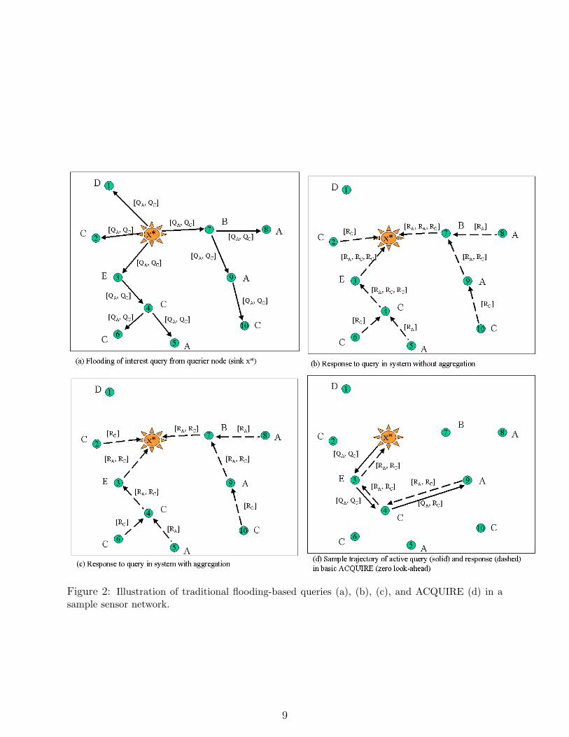
Figure 2: Illustration of traditional flooding-based queries (a), (b), (c), and ACQUIRE (d) in asample sensor network.

9

Figure 3: Illustration of ACQUIRE with a one-hop lookahead (d = 1). At each step of theactive query propagation, the node carrying the active query employs knowledge gained due tothe triggered updates from all nodes within d hops in order to partially resolve the query. As dbecomes larger, the active query has to travel fewer steps on average, but this also raises the updatecosts. When d becomes extremely large, ACQUIRE starts to resemble traditional flooding-basedquerying.

2. All the sensors have the same transmission range.

3. The nodes are stationary and do not fail.

We model the size of a sensor’s neighborhood (the number of nodes within d hops) as afunction of d, f(d), which is assumed to be independent of the particular node in question3.We also assume that all possible queries Q are resolvable by this network (i.e. can beresponded to by at least one node in the network).

Mechanism of Query Forwarding:Initially, let sensor x∗ be the querier that issues a query Q consisting of M subqueries4. Let

3The size of the neighborhood is actually a measure of the number of different variables tracked by a node’sneighborhood. For the sake of simplicity, we assume that each sensor tracks a single variable. However, thisassumption does not affect the conclusions of our analysis

4One way to think of the size of the complex query M is to treat it as a “batch” parameter which effects atradeoff between latency for batching and the latency and energy for query completion. Imagine independentsub-queries arrive at the central node at a fixed rate, then the time to put together a single batched queryincreases linearly with M , while the expected query completion time and energy increases only sub-linearlywith M (as shown in section 4). In general the larger M is, the worse the batching latency, but better theaverage query completion time and energy expenditure (assuming subsequent queries are only sent out afterthe previous one has terminated).

10

d be the look-ahead parameter i.e each sensor can request information from sensors d hopsaway from it. In general when a sensor x gets a query it does the following:

1. Local Update: If its current information is not up-to-date, x sends a request to allsensors within d hops away. This request is forwarded hop by hop. The sensors whoget the request will then forward their information to x. Let the energy consumed inthis phase be Eupdate. Detailed analysis of Eupdate will be done in section 4.3.

2. Forward: After answering the query based on the information obtained, x then forwardsthe remaining query to a node that is chosen randomly from those d hops away.

Since the update is only triggered when the information is not fresh, it makes sense to try toquantify how often such updates will be triggered. We model this update frequency by anaverage amortization factor c, such that an update is likely to occur at any given node onlyonce every 1

cqueries. In other words the cost of the update at each node is amortized over

1c

queries, where c ≤ 1. For example, if on average an update has to be done once every 100queries, c = 0.015.

After the query is completely resolved, the last node which has the query returns the com-pleted response6 to the querier x∗ along the reverse path 7. We use α to denote the expectednumber of hops from the node where the query is completely resolved to x∗.

Let SM be the average number of steps to answer a query of size M . Thus, the averageenergy consumed to answer a query of size M with look-ahead d can be expressed as follows:

Eavg = (cEupdate + d)SM + α (1)

Now, if d = D, where D is the diameter of the network, x∗ can resolve the entire queryin one step without forwarding it to any other node. However, in this case, Eavg will beconsiderably large. On the other hand, if d is too small, a larger number of steps SM will berequired. In general, SM reduces with increasing d, while Eupdate increases with increasing d.It is therefore possible, depending on other parameters, that the optimal energy expenditureis incurred at some intermediate value of d. One of the main objectives of our analysis is toanalyze the impact of parameters such as M , N , c, and d upon the energy consumption Eavg

of ACQUIRE.

5It might be convenient to think of every datum having a time duration during which it is valid. Duringthis period, all queries for the corresponding variable could be answered from the value cached from previoustriggered updates. E.g. a sample bird call might have a longer validity period than a temperature reading.

6We note that it also makes sense to return partial responses back to the querier, as each sub-query isresolved along the way. This would reduce the energy and time costs of carrying partial responses alongwith the partial query. Our analysis thus overestimates the energy cost, and could be tightened further inthis regard.

7If additional unicast or geographic routing information is available, the completed response can also besent back along the shortest path back from the final node to the querier.

11

4.2 Steps to Query Completion

In this section, we present a simple analysis of the average number of steps to query com-pletion as a function of M , N and f(d). A more detailed analysis is in section 12 in theAppendix.

4.2.1 First-order Analysis

Consider the following experiment. Each sensor tracks a value chosen between 1 and N withequal probability. Fetching information from each sensor can be thought of as a trial. Definea “success” as the event of resolving any one of the remaining queries. Thus, if there arecurrently M queries to be resolved, then the probability of success in each trial is p = M

N

and the probability of failure is q = N−MN

. The number of trials till the first success i.e. thenumber of sensors from which information has to be fetched till one of the queries can beanswered is a geometric random variable. Thus, the expected number of trials till the firstsuccess is 1

p= N

M. Now the whole experiment can be repeated again with one less query.

Thus, now, p = M−1N

and q = N−M+1N

. The expected number of trials till the first success(i.e. another query being answered) is N

M−1and so on.

Define the following:

1. σM = The number of trials till M successes i.e. the resolution of the entire query.

2. Xi: The number of trials (counted from the (i− 1)th success) till the ith success.

σM and Xi’s are random variables.Now,

σM =M∑i=1

Xi (2)

By linearity of expectation,

E(σM) =M∑i=1

E(Xi) (3)

E(σM) = N

M∑i=1

1

M − i + 1(4)

Now,∑M

i=11

M−i+1= H(M) where H(M) is the sum of the first M terms of the harmonic

series.It is known that H(M) ≈ ln(M) + γ, where γ = 0.57721 is the Euler’s constant. Thus,

E(σM) ≈ N(ln M + γ) (5)

12

Now, since we consider fetching information from f(d) sensors as 1 trial (step) rather thanf(d) trials (steps)8:

SM =E(σM)

f(d)≈ N(ln M + γ)

f(d)(6)

Eqn. 6 expresses the average number of steps to query completion (SM) as a function of thetotal number of variables (N), the query size (M) and the neighborhood size (f(d)).

To answer more complex questions like “what is the probability that a complex query canbe reduced in size in a single step?”, we formulate the query forwarding process as a MarkovChain. Detailed analysis of this Markov Chain is in section 12 in the Appendix.

4.3 Local Update Cost

The energy spent in updating the information at each active node that is processing theactive query Eupdate can be calculated as follows:Assume that the query Q is at the active node x. Given a look-ahead value d, x canrequest information from sensors within d hops away. This request will be forwarded by allsensors within d hops except those that are exactly d hops away from x. Thus the numberof transmissions needed to forward this request is the number of nodes within d − 1 hopswhich is f(d− 1). The requested sensors will then forward their information to x. Now, theinformation of sensors 1 hop away will be transmitted once, 2 hops away will be transmittedtwice,... d hops away will be transmitted d times. Thus,

Eupdate = (f(d− 1) +d∑

i=1

iN(i)) (7)

where N(i) is the number of nodes at hop i. N(i) will be determined later in section 4.4.

4.4 Total Energy Cost

We make the assumption that each active node forwards the resolved query to another nodethat is exactly d hops away, requiring d transmissions. Hence the average energy spent inanswering a query of size M is given as follows:

Eavg = (cEupdate + d)SM + α (8)

8Here, we make an assumption that f(d) new nodes will be encountered at every node where the queryis forwarded. However, due to overlap, the number of new nodes actually encountered might be a fractionof f(d) i.e. (1− δ)f(d), where 0 < δ < 1, is a measure of the average overlap of the neighborhoods of nodeshandling the query. It depends on algorithm used to route the query. For ACQUIRE to perform efficiently,this overlap should be small.

13

where α is the expected number of hops from the node where the query is completely resolvedto the querier x∗.9 This is the cost of returning the completed response back to the queriernode. This response can be returned along the reverse path in which case α can be atmostdSM . Thus,

Eavg = (cEupdate + 2d)SM (9)

4.4.1 Special Case: d = 0 - Random Walk

If the look-ahead d = 0, the node x will not request for updates from other nodes. x will tryto resolve the query with the information it has, and will forward the query to a randomlychosen neighbor. Thus, in this case, ACQUIRE reduces to a random walk on the network.On an average it would take E(σM) steps to resolve the query and E(σM) steps to returnthe resolved query back to the querier x∗. Thus,

Eavg = 2E(σM) (10)

4.5 Optimal Look-ahead

As mentioned in section 4.4,

Eavg = {(f(d− 1) +d∑

i=1

iN(i))c + 2d}SM (from Eqn.7 and 9)

≈ {(f(d− 1) +d∑

i=1

iN(i))c + 2d}N(ln M + γ)

f(d)(from Eqn.6) (11)

If we ignore boundary effects, it can be shown that f(d) = (2d(d + 1)) + 1 for a grid10

Also,

N(i) = f(i)− f(i− 1)

= 2i(i + 1)− 2(i− 1)i

= 4i (12)

i.e. the number of nodes exactly i hops away from a node x on a grid is 4i. Thus,

Eavg ≈ {(2(d− 1)(d) + 1 +d∑

i=1

4i2)c + 2d} N(ln M + γ)

(2(d)(d + 1)) + 1

9Here, we are actually over-estimating Eavg by an additive amount of SM as the query will not beforwarded at the last step, but will be returned back to the querier.

10Here we assume that at every node handling the query, there are f(d) new nodes available in theneighborhood i.e. the query is routed such that there is minimal overlap between the neighborhoods ofnodes handling the query. We will see the effect of overlap in simulation results.

14

≈ {(2(d− 1)(d) + 1 +4

6(d)(d + 1)(2d + 1))c + 2d} N(ln M + γ)

(2(d)(d + 1)) + 1

≈ {cN(ln M + γ)

3

4d3 + 12d2 − 4d + 3

2d2 + 2d + 1+ N(ln M + γ)

2d

2d2 + 2d + 1} (13)

To find the value of d (as a function of c, N and M) that minimizes the Eavg, we differentiatethe above expression w.r.t. d and set the derivative to 0. We get the following:

2

3

(N ln M + γ)(4cd4 + 8cd3 + 22cd2 + 6cd− 5c− 6d2 + 3)

(2d2 + 2d + 1)2= 0

4cd4 + 8cd3 + 22cd2 + 6cd− 5c− 6d2 + 3 = 0 (14)

Thus, the optimal look-ahead d∗ depends on the amortization factor c and is independentof M and N .If d = 0:

Eavg ≈ 2N(ln M + γ) (from Eqn. 5 and 10) (15)

In this case, since no look-ahead is involved, Eavg is independent of c and d.

4.6 Effect of c on ACQUIRE

We first analytically study the behavior of ACQUIRE for different values of c and d and findthe optimal look-ahead d∗ for a given c, M and N . We used Eqn. 13 derived in section 4.5.N was set to 100 and M was set to 20. We varied c from 0.001 to 1 in steps of 0.001 and dfrom 1 to 10. For d = 0, Eavg is independent of c and d as shown by Eqn. 15 in section 4.5.

Figure 4 shows the energy consumption of the ACQUIRE scheme for different amortizationfactors and look-ahead values. Let d∗ be the look-ahead value which produces the minimumaverage energy consumption. It appears that d∗ significantly depends on the amortizationfactor.

Figure 5 shows that as the amortization factor c decreases, d∗ increases. i.e. as the queryrate increases and the network dynamics decreases it is more energy-efficient to have a higherlook-ahead. This is intuitive because in this case, with a larger look-ahead, the sensor canget more information that will remain stable for a longer period of time which will help itto answer subsequent queries. Thus, in our study, for very small c (0.001 ≤ c ≤ 0.01), d∗

is as high as possible ( d∗ = 10 ). On the other hand, for 0.08 ≤ c < 0.9 (approx.), themost energy efficient strategy is to just request information from the immediate neighbors(d = 1). It is also seen that there are values of c in the range from [0.001, 0.1] such thateach of 1, 2, ...10 is the optimal look-ahead value. If c ≥ 0.9 (approx.), the most efficientstrategy for each node x is to resolve the query based on the information it has (withouteven requesting for information from its neighbors i.e. d = 0).

15

Figure 4: Effect of c and d on the Average Energy Consumption of the ACQUIRE scheme.Here, N = 100 and M = 20

Figure 5: Effect of c on d∗ for N = 100 and M = 20. The x-axis is plotted on a log scale.

16

5 Analysis of Alternative Approaches

In this section, we present the energy cost of expanding ring search and flooding based querymechanisms. While the expanding ring search is not currently implemented in any sensorquerying protocols we are aware of, it is a better baseline for comparison than the clearlyinefficient flooding-based querying, as far as one-shot queries are concerned.

5.1 Expanding Ring Search (ERS)

In an Expanding ring search, at stage 1, the querier x∗ will request information from allsensors exactly one hop away. If the query is not completely resolved in the first stage, x∗

will send a request to all sensors two hops away in the second stage. Thus, in general atstage i, x∗ will request information from sensors exactly i hops away. The average number ofstages tmin taken to completely resolve a query of size M can be approximately determinedby the First order analysis in section 4.2.1:

tmin∑i=1

N(i) = N(ln M + γ) (from Eqn.5)

4

tmin∑i=1

i = N(ln M + γ) (from Eqn.12)

2tmin(tmin + 1) = N(ln M + γ)

2(tmin)2 + 2tmin −N(ln M + γ) = 0 (16)

tmin can be determined by solving the above quadratic equation (taking the ceiling if neces-sary to get tmin as an integer).

In ERS, at stage i, all nodes within i−1 hops of the querier x∗ will forward the x∗’s request.Let Navg(i) be the expected number of nodes at hop i that will resolve some sub-query. Theresponse from these nodes will be forwarded over i hops. There are a total of tmin stages.Thus, the total update cost is given as follows:

Eupdate =

tmin∑i=1

(f(i− 1) + iNavg(i))

=

tmin∑i=1

f(i− 1) +

tmin∑i=1

iNavg(i) (17)

Navg(i) can be computed as follows:At the ith step, f(i− 1) nodes would already have been requested for their information. Theexpected number of queries resolved Mr(i− 1) before the ith step can be given as follows:

f(i− 1) = N(ln(Mr(i− 1)) + γ) (from Eqn.5)

Mr(i− 1) = ef(i−1)

N−γ (18)

17

Thus, in the ith step, the probability of “success” is given by

pi =M −Mr(i− 1)

N(19)

Thus, in step i, the expected number of nodes that will resolve some sub-query is given by:

Navg(i) = N(i)pi (substituting pi for p in Eqn.23)

= N(i)(M − e

f(i−1)N

−γ

N) (20)

Since the query is not forwarded to any other node,

Eavg = Eupdatec (substituting d = 0, α = 0, SM = 1 in Eqn.8)

= (

tmin∑i=1

(2i(i− 1) + 1) +

tmin∑i=1

iN(i)(M − e

f(i−1)N

−γ

N))c

= (1

3(tmin)(tmin + 1)(2tmin + 1)− (tmin)(tmin + 1) + tmin +

tmin∑i=1

iN(i)(M − e

f(i−1)N

−γ

N))c

= (2

3(tmin)(tmin + 1)(tmin − 1) + tmin +

tmin∑i=1

iN(i)(M − e

f(i−1)N

−γ

N))c (21)

5.2 Flooding-Based Query (FBQ)

In FBQ, the querier x∗ sends out a request to all its immediate neighbors. These nodes inturn, resolve the query as much as possible based on their information and then forwardthe request to all their neighbors and so on. Thus, the request reaches all the nodes in thenetwork.

In general, as mentioned in Eqn. 8 from section 4.4,

Eavg = (cEupdate + d)SM + α

(22)

In FBQ:

1. The request for triggered updates will have to be sent as far as R hops away from thequerier x∗ (near the center of the grid) where R is the “radius” of the network i.e. themaximum number of hops from the center of the grid.

2. d = 0, as the query is not forwarded.

3. α = 0, as the query is completely resolved at the origin of the query itself.

4. SM = 1.

18

Let Navg(i) be the expected number of nodes at hop i, that can resolve some part of thequery. This can be determined along similar lines as in section 4.2.1:As before, consider the fetching of information from a sensor as a “trial”. In each “trial”,the probability of success is p = M

Nand the probability of failure is q = N−M

N. The number

of successes is a binomial random variable. The total number of “trials” at hop i is N(i).Thus, the expected number of successes at hop i is given by

Navg(i) = N(i)p (23)

The response of each of the Navg(i) nodes will be forwarded over i hops.Thus, for FBQ, Eavg is given as follows:

Eavg = (f(R) +R∑

i=1

iNavg(i))c

= (f(R) +R∑

i=1

iN(i)M

N)c

= (f(R) +M

N

R∑i=1

iN(i))c

= (2R(R + 1) + 1 +2

3

M

NR(R + 1)(2R + 1))c (24)

For a grid with X nodes, R =√

X. Thus, For a given M , N and c, Eavg ∝ X3/2.

6 Comparison of ACQUIRE, ERS and FBQ

6.1 Effect of c

These schemes were analytically compared across different values of c chosen in the range of[0.001, 1] as in section 4.6. The total number of nodes X was 104. For ACQUIRE, the look-ahead parameter was set to d∗ for a given value of c. We refer to this version of ACQUIREas ACQUIRE∗. Eqn. 21 from section 5.1, Eqn. 24 from section 5.2 and Eqn. 13 fromsection 4.5 (with d = d∗) were used in the comparative analysis. For the initial comparisons,N = 100 and M = 20. Using these values for M and N in Eqn. (16) from section 5.1, weobtain tmin = 13. This value of tmin is then used in Eqn. 21.

As figure 6 shows that ACQUIRE with look-ahead 0 (i.e. random walk) performs at leastas worse as ACQUIRE with the optimal look-ahead (ACQUIRE∗). ACQUIRE∗ seems tooutperform ERS for higher values of the amortization factor. Moreover at c = 1, ACQUIREgives about a 60% energy savings over ERS. In the case of N = 100 and M = 20, ACQUIRE∗

outperforms ERS if c ≥ 0.08 (approx.). In this case, d∗ = 1 as shown by figure 5.

19

Figure 6: Comparison of ACQUIRE∗, ERS, ACQUIRE with d = 0 and FBQ with energyon a log scale (left) and a linear scale (right). (For N = 100 and M = 20)

Figure 7: Comparison of ACQUIRE∗, ERS, ACQUIRE with d = 0 and FBQ with energyon a log scale (left) and on a linear scale (right) (for N = 160 and M = 50).

20

However, it is not always the case that ACQUIRE∗ outperforms ERS only with d∗ = 1. IfN = 160 and M = 50, tmin = 19 (from Eqn. 16). With these values of M and N as shownby the figure 7, ACQUIRE∗ outperforms ERS if c ≥ 0.06 (approx.). In this case, d∗ = 2as shown by figure 5. Moreover in this case as figure 7 shows, for c > 0.2, even ACQUIREwith d = 0 would outperform ESR. Again, for c = 1, ACQUIRE∗ achieves more than 75%energy savings over ERS.

As figure 6 shows, FBQ, on an average, incurs the worst energy consumption which is severalorders of magnitude higher than the other schemes. This is mainly because of a very largenumber of nodes (X = 104) used in our study.

From, the above analysis, it seems that the relative query size (MN

), seems to have a significantimpact on the performance of ACQUIRE and ERS. Hence we analyze this effect in section6.2. FBQ always incurs an order of magnitude worse energy consumption, and hence we donot study the impact of the relative query size on FBQ.

6.2 Effect of MN

Intuitively, for a given N , as M is increased, ERS has to “expand” the ring more, whileACQUIRE will take more steps to resolve the query. In this section, we fix N at 100 andlet M to take the values of 10, 20, 40, 60, 80 and 100. For each value of M

N, we observe the

performance of ACQUIRE∗ and ERS for c = 0.05, c = 0.2 and c = 1. For ERS, the valuesof tmin for these values of M

Nare 12, 13, 15, 15, 16 and 16 respectively.

As the figures 8 shows, the average energy consumed to resolve a complex query increaseswith increasing M for a given N . For c = 0.05, ERS performs better than ACQUIRE∗

when MN≤ 0.5, while in the other cases ACQUIRE∗ outperforms ERS across all the amor-

tization factors and relative query sizes in our study. In these cases, the energy savings ofACQUIRE∗ over ERS are seen to range as high as 85% (e.g. when c = 1, M

N= 1).

Thus, both c and MN

seem to have a significant impact on the performance of ACQUIRE andERS. As c increases and M

Nincreases, ACQUIRE achieves significant energy savings over

ERS (and FBQ).

7 Validation of the Analytical Models

In this section, we validate our analytical models by conducting some high level simulations.Specifically, our objectives were the following:

1. Validate the effect of c on ACQUIRE.

2. Validate the comparisons between ACQUIRE, ERS and FBQ for different values of c.

21

(a) c = 0.05

(b) c = 0.2

(c) c = 1

Figure 8: Comparison of ACQUIRE∗, and ERS (N = 100) with respect to MN

for differentamortization factors.

22

3. Perform a relative comparison between ACQUIRE and ERS across different relativequery sizes (M

N).

As we shall show, our simulation results are more or less in line with our analysis. The minordifferences can be ascribed to factors such as overlap in the query trajectory and boundaryeffects that are not modelled in our analysis.

7.1 Simulation Setup

Our setup consists of a 100m x 100m grid with 104 sensors placed at a distance of 1m fromeach other. The communication range of each sensor is 1m. The total number of variablesin our simulations is set to 100. For all the querying mechanisms, a query is always injectedat the center of the grid i.e. at sensor (50, 50). We ran our simulations on 1000 queries. Inorder to take advantage of the caching, the query was made to follow a fixed trajectory inACQUIRE. The first query out of the set of 1000 queries fixes the trajectory, while all thesubsequent queries follow the same trajectory.

Our analysis assumed that there are no loops in the query trajectory. It turned out thatthis can very effectively achieved by ACQUIRE’s local update phase at no additional cost.Each node maintains a flag called queried. Whenever a node is requested for an update, itsets this flag to true. Subsequently, whenever a node is requested for an update, it sendsthe value of the queried flag along with the variable. Once an active node has processed thequery based on the information in its neighborhood, it forwards the remaining query to anode at d hops whose queried flag is false. Using this mechanism, most of our simulationshave no loops in the query trajectory for d ≥ 1. However, for the random walk (d = 0),there is no local update phase. Hence, in this case, there are loops in the query trajectorycausing the random walk to revisit nodes. These loops lead to a 45 − 50% degradation inthe performance11 as we will show in section 7.3. For ERS and FBQ, there is no trajectoryas the query is never forwarded to other nodes.

7.2 Effect of c on ACQUIRE

In our simulations, we used 5 different values of c i.e. 0.001, 0.01, 0.05, 0.2 and 1. Wesimulated the c as follows: Each variable has a validity time of 1

c, where time is taken

to be the number of queries. E.g. If c = 0.001, each variable is valid for 1000 queries.During this validity period, all queries for that particular variable can be answered using thecached copies. Beyond the validity period, the active node has to “refresh” variables from its“neighborhood”. For each value of c, simulations were run using 100 different random seeds.

11The analysis of ACQUIRE with d = 0 case assumed that there is no looping. The significant performancedegradation observed in simulations suggests that the use of straightening algorithms such as those describedin [21] or geographically directed trajectories such as routing on curves [20] is necessary when ACQUIRE isused with d = 0 in practice.

23

Figure 9: Effect of c on d∗ by simulations (N = 100 , M = 20). Compare with theoreticalcurves in figure 4

In each run, we used 1000 queries, each consisting of 20 sub-queries (or variables). For eachrun, the generated queries were stored in a query-file. At the same time the values chosenby each sensor were also stored in a grid-file for each run. The number of transmissions wereaveraged across all these runs for a given c.

As figure 9 shows, with increasing c, the optimal look-ahead d∗ decreases. This concurs withour analysis in section 4.5. The simulations show that for c = 0.001, 0.01, the d∗ = 10 (largestpossible value used in our simulations), which is the same as shown by our analytical curvesin figure 4. For c = 0.05, d∗ = 5 from simulations, while the analytical d∗ = 3. For c = 1,from simulations d∗ = 1, while from the analytical d∗ = 0. This is because in simulations, asmentioned in section 7.1, ACQUIRE with d = 0 has loops in its trajectory, which degradesits performance by around 45− 50%.

7.3 Comparison of ACQUIRE, ERS and FBQ

7.3.1 Effect of c

For both ERS and FBQ, we use the same simulation setup as ACQUIRE. For both thesemechanisms, we simulate 100 different runs. Each run consists of 1000 queries each containing20 sub-queries. In each run, we use the query-files, grid-files and same values of c describedin section 7.2.

24

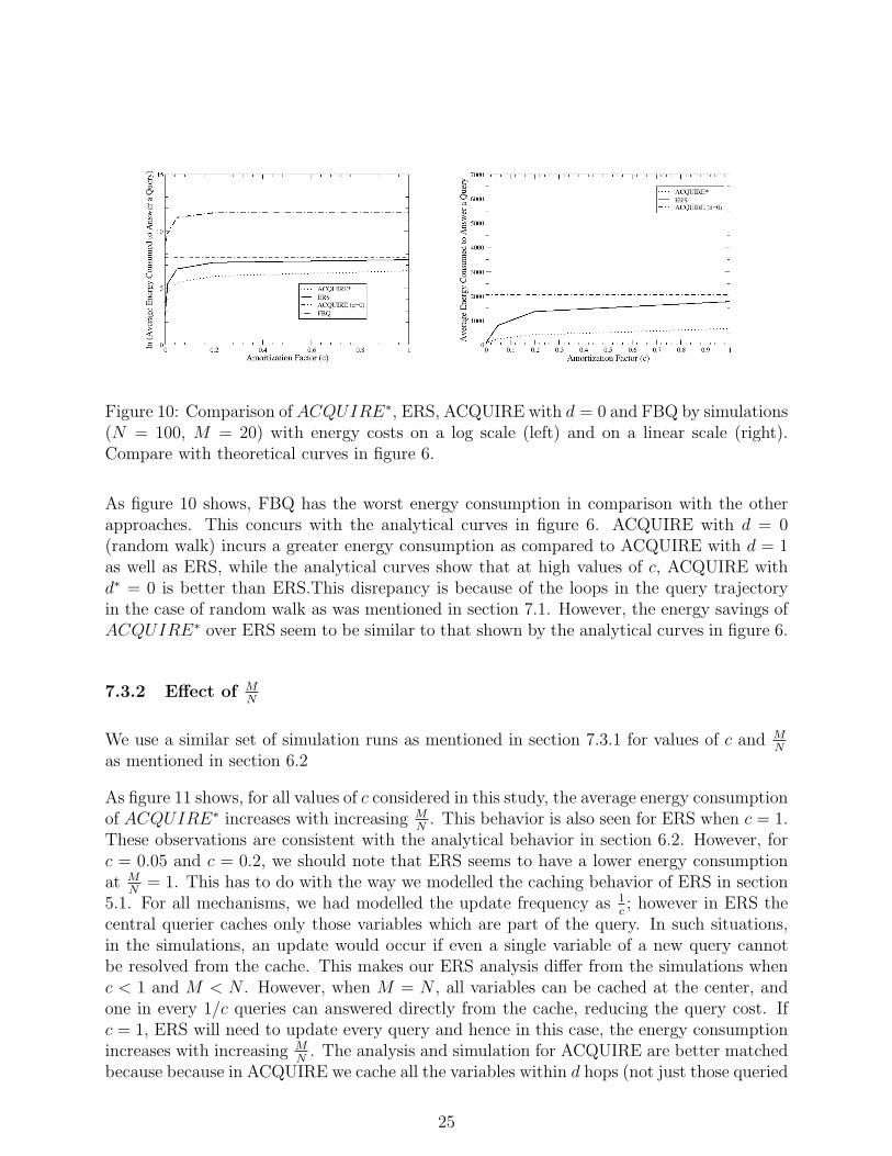
Figure 10: Comparison of ACQUIRE∗, ERS, ACQUIRE with d = 0 and FBQ by simulations(N = 100, M = 20) with energy costs on a log scale (left) and on a linear scale (right).Compare with theoretical curves in figure 6.

As figure 10 shows, FBQ has the worst energy consumption in comparison with the otherapproaches. This concurs with the analytical curves in figure 6. ACQUIRE with d = 0(random walk) incurs a greater energy consumption as compared to ACQUIRE with d = 1as well as ERS, while the analytical curves show that at high values of c, ACQUIRE withd∗ = 0 is better than ERS.This disrepancy is because of the loops in the query trajectoryin the case of random walk as was mentioned in section 7.1. However, the energy savings ofACQUIRE∗ over ERS seem to be similar to that shown by the analytical curves in figure 6.

7.3.2 Effect of MN

We use a similar set of simulation runs as mentioned in section 7.3.1 for values of c and MN

as mentioned in section 6.2

As figure 11 shows, for all values of c considered in this study, the average energy consumptionof ACQUIRE∗ increases with increasing M

N. This behavior is also seen for ERS when c = 1.

These observations are consistent with the analytical behavior in section 6.2. However, forc = 0.05 and c = 0.2, we should note that ERS seems to have a lower energy consumptionat M

N= 1. This has to do with the way we modelled the caching behavior of ERS in section

5.1. For all mechanisms, we had modelled the update frequency as 1c; however in ERS the

central querier caches only those variables which are part of the query. In such situations,in the simulations, an update would occur if even a single variable of a new query cannotbe resolved from the cache. This makes our ERS analysis differ from the simulations whenc < 1 and M < N . However, when M = N , all variables can be cached at the center, andone in every 1/c queries can answered directly from the cache, reducing the query cost. Ifc = 1, ERS will need to update every query and hence in this case, the energy consumptionincreases with increasing M

N. The analysis and simulation for ACQUIRE are better matched

because because in ACQUIRE we cache all the variables within d hops (not just those queried

25

(a) c = 0.05

(b) c = 0.2

(c) c = 1

Figure 11: Comparison of ACQUIRE∗ and ERS by simulations (N = 100) with respect toMN

for different amortization factors. Compare with theoretical curves in figure 8

26

for).

From simulations, at MN

= 1, c = 0.05, ERS performs better than ACQUIRE∗. On theother hand, for all other values of c used in our study, ACQUIRE∗ outperforms ERS acrossall relative query sizes. The energy savings of ACQUIRE∗ over ERS is around 65% forc = 0.02 (for all values M

N< 1) and c = 1 (for all values of M

N).

Our analysis of the energy cost of ACQUIRE, ERS and FBQ by analytical models andsimulations illustrate that ACQUIRE achieves significant energy savings for moderate tohigh values of c depending on the relative query size. Do these energy savings come at acost? We attempt to answer this question in the next section by modelling the averageresponse latency incurred by these mechanisms.

8 Latency Analysis

In this section, we attempt to analytically compare the average latency in obtaining a re-sponse to a query by these 3 mechanisms. The metric for latency that we examine is theexpected number of sequential transmissions required before a response is obtained to a givenquery. We should note that this is a network layer analysis that does not take into accountMAC delay due to contentions.

8.1 ACQUIRE

In this section, we analyze the latency incurred by ACQUIRE∗ in answering a query.

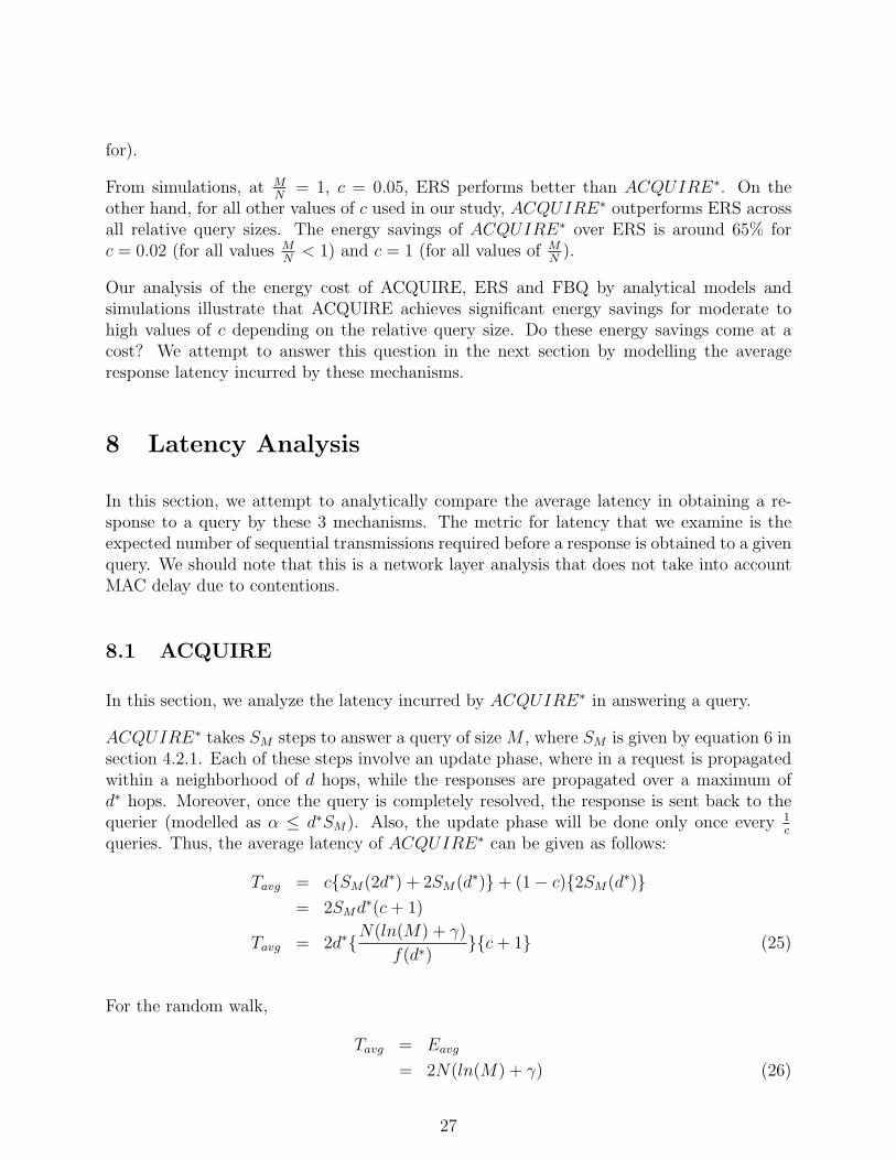
ACQUIRE∗ takes SM steps to answer a query of size M , where SM is given by equation 6 insection 4.2.1. Each of these steps involve an update phase, where in a request is propagatedwithin a neighborhood of d hops, while the responses are propagated over a maximum ofd∗ hops. Moreover, once the query is completely resolved, the response is sent back to thequerier (modelled as α ≤ d∗SM). Also, the update phase will be done only once every 1

c

queries. Thus, the average latency of ACQUIRE∗ can be given as follows:

Tavg = c{SM(2d∗) + 2SM(d∗)}+ (1− c){2SM(d∗)}= 2SMd∗(c + 1)

Tavg = 2d∗{N(ln(M) + γ)

f(d∗)}{c + 1} (25)

For the random walk,

Tavg = Eavg

= 2N(ln(M) + γ) (26)

27

8.2 ERS

In ERS, on an average the ring has to expand till tmin hops to get updates, where tmin isgiven by Eqn. 16. The latency in executing a ring of size x is 2x, x for the request and x forthe reply. Moreover, these updates are sought once every 1

cqueries. The remaining fraction

of the queries are answered from the cached responses (which has a latency of 0). Thus, theaverage latency in ERS is given as follows:

Tavg = c{tmin∑i=1

2i}+ (1− c){0}

= c(tmin)(tmin + 1) (27)

8.3 FBQ

Similar to the latency analysis for ERS, in FBQ, the request for updates has to be forwardedfor tmin hops on an average before all the sub-queries can be answered. Thus, the latencyfor issuing the request and getting the updates is 2tmin. The updates are issued once every1c

queries. For the remaining fraction, the queries are answered from the cache (incurring alatency of 0). Thus, the average latency incurred by FBQ is

Tavg = 2ctmin (28)

Figure 12 shows the analytical comparison of ACQUIRE∗, ERS and FBQ when N = 100,M = 20 and X = 104. The average latency seems to increase from FBQ to ERS toACQUIRE∗ across all values of the amortization factor c. The latency for both FBQand ERS increases linearly with c as is evident from Eqn. 28 and Eqn. 27 respectively.Interestingly, the latency in ACQUIRE∗ has a piece-wise linear behavior with respect to c.This is because the changing c alters d∗ discontinuously which in turn alters d∗

f(d∗)i.e. the

slope of the line Tavg as shown by Eqn. 25. At the point where the latency is constant withrespect to c, ACQUIRE∗ resembles a random walk (d = 0). The difference in the latencyis significant (around 500 transmissions), when d∗ for ACQUIRE goes from 1 to 0.

9 Storage Requirements

Our analysis in this paper assumes that all the mechansims i.e. ACQUIRE, ERS and FBQutilize caching to answer queries. We now attempt to quantify the storage space requirementsfor the cache across these approaches.

In ACQUIRE, an active node requests an update from its “neighborhood” consisting of f(d)(with d = d∗). In the worst case, the each of these f(d) variables might be distinct, thusneeding O(f(d)) storage space. For a grid and for most reasonable topologies, note that

28

Figure 12: Comparison of the latency incurred by ACQUIRE∗, ERS and FBQ. Here, N =100, M = 20, X = 104, tmin = 13. The x-axis is plotted on log-scale.

f(d) would be polynomial in d. ACQUIRE distributes the cache at nodes which handle thequery. In the case of ACQUIRE, the storage requirements depend on the optimal lookaheadd∗, which in turn is dependent on the data dynamics. Higher c, higher the data dynamics,lower the optimal lookahead d∗, smaller the cache requirements at each node.

For ERS and FBQ, each querier (there may be only one, always located at the same node)requires a cache that is between O(M) and O(N) in size. This is because this querier nodemust cache all responses to all valid queries.

10 Discussion and Future Work

Partly for ease of analysis, we have described and modelled a very basic version of theACQUIRE mechanism in this paper. One of our major next steps is to convert ACQUIREinto a functional protocol that can be validated on an experimental sensor network test-bed. There are a number of ways in which our analysis can be improved, and a number ofadditional design issues need to be considered in our future work, some of which we outlinehere.

Our analytical model of ACQUIRE assumes that the query packet is always of a fixed sizeconsisting of all the individual sub-queries and their responses. The entire packet circulatesin the network till the answer to the last query is obtained. The packet is then sent back to

29

the querier. This simplifies the analysis as we need to only count the number of transmissionsin order to quantify Eavg. However, it may be more efficient to send the answers to sub-queries to the querier node as and when they are obtained. Our analysis could be tightenedto take this into consideration.

The efficiency of ACQUIRE can also be improved if the neighborhoods of the successiveactive nodes in the query trajectory have minimal overlap. This may potentially be bestaccomplished by using some deterministic trajectory as opposed to random walks, possiblymaking use of additional topological or geographical information. These would also aid inminimizing inefficiency due to the walk revisiting nodes (looping). Guided trajectories mayalso be helpful in dealing with non-uniform data distributions, ensuring that active queriesspend most time in regions of the network where the relevant data are likely to be. Inthe analysis, we ignored the issue of overlap (although this was taken into account in thesimulations we presented).

One interesting result of our analysis is that the performance of ACQUIRE and the optimalchoice of the look-ahead parameter d∗ are functions of the amortization factor c and (some-what surprisingly) independent of M , N , and the total number of nodes X. This lends itselfto the possibility of using distributed algorithms in which localized estimates of c are used todetermine the value of d at each step without global knowledge of system parameters. Thiswould significantly improve the scalability of ACQUIRE.

As presented here, ACQUIRE is meant to be used in situations where there is replicateddata. At the very least there should be one node in the network that can resolve eachcomponent sub-query. One way to deal with other situations might be to equip the activequeries with a time-to-live (TTL) field which is decremented at each hop. This would permitACQUIRE to gracefully terminate with a negative response if a solution is not found withina reasonable period of time, to be followed up (for example) by a flooding-based query.

Our analysis has assumed a regular grid topology. This helped us in gaining considerableinsight into the performance of ACQUIRE, ERS and FBQ. In reality the topology of asensor network might not only be irregular but also dynamic, due to failures and mobility.Exploring the behavior of ACQUIRE on such topologies is a focus of our ongoing effort. Weshould mention, however, that our results do already have some generality in this regard: solong as a reasonable model for f(d) can be developed for the network topology, the analysispresented here can be extended in a straightforward manner.

In our modelling we have only counted the number of transmissions for energy costs, althoughit is true that receptions can also influence energy consumption. This is the case especiallyfor broadcast messages, where there’s no channel reservation and all the direct neighborsreceive the message. We believe that some of the alternatives to active querying, suchas FBQ and ERS will in fact incur even more energy consumption under an energy modelthat incorporates receptions because all their query messages are broadcast. Moreover, thesebroadcasts would also lead to an increased latency in FBQ and ERS due to higher contention.We would like to examine such richer energy cost models in the future.

30

In our analysis of delay, we looked only at response latency at the network layer (by examiningthe number of maximum sequential transmissions required). These results must be takenwith a grain of salt, because they do take into account MAC-layer delay. For broadcast-basedquerying techniques such as FBQ and ERS, there could be far greater MAC layer contentionthan in ACQUIRE. This deserves worth further investigation.

We have also ignored the possibility of aggregate queries in this paper. Our assumption hasbeen that each sub-query is independent. This would be another direction for future work.

11 Conclusions

In this paper, we have proposed ACQUIRE - a novel mechanism for data extraction in energy-constrained sensor networks. The key feature of ACQUIRE is the injection of active queriesinto the network with triggered local updates. We first categorized sensor network querytypes and identified those for which ACQUIRE is likely to perform in an energy-efficientmanner: complex, one-shot, non-aggregate queries for replicated data.

We have developed a fairly sophisticated mathematical model that allows us to analyticallyevaluate and characterize the performance (in terms of energy costs and response latency)of ACQUIRE, as well as alternative techniques such as flooding-based queries (FBQ) andexpanding ring search (ERS). As far as we are aware, there are very few similar results in theliterature that provide similar mathematical characterizations of the performance of querytechniques for sensor networks. We validated our analysis through extensive simulations andalso identified ways in which the models can be extended and improved.

In our analysis we defined an amortization factor c to meaningfully capture the relationshipbetween the query rate and data dynamics. When c is low, more queries can be processedin the time that a given datum remains “fresh.” Our analysis revealed that this parameterhas a significant impact on the energy costs of cached update schemes such as the one usedin ACQUIRE. Indeed, we showed that the optimal look-ahead in ACQUIRE depends solelyupon c, not on other parameters such as the size of the network or the size of the queries.

We found that ACQUIRE with optimal parameter settings outperforms the other schemes forcomplex, one-shot queries in terms of energy consumption. Specifically, optimal ACQUIREperforms many orders of magnitude better than flooding-based schemes (such as DirectedDiffusion) for such queries in large networks. We also observed that optimal ACQUIREcan reduce the energy consumption by more than 60− 75% as compared to expanding ringsearch (in highly dynamic environments and high query rates). The energy savings arehighest when c is high and NlnM is high. However, this energy savings come at the cost ofincreased average latency in answering a query.

To conclude, we believe that there is no one-size-fits-all answer to the question: “How do weefficiently query sensor networks?” We propose ACQUIRE as a highly scalable technique,energy-efficient at solving complex one-shot queries for replicated data. We argue that

31

ACQUIRE deserves to be incorporated into a portfolio of query mechanisms for use in real-world sensor networks.

References

[1] D. Estrin, L. Girod, G. Pottie, and M. Srivastava, “Instrumenting the World with Wireless Sen-sor Networks,” International Conference on Acoustics, Speech and Signal Processing (ICASSP2001), Salt Lake City, Utah, May 2001.

[2] J. Warrior, “Smart Sensor Networks of the Future,” Sensors Magazine, March 1997.

[3] G.J. Pottie, W.J. Kaiser, “Wireless Integrated Network Sensors,” Communications of the ACM,vol. 43, no. 5, pp. 551-8, May 2000.

[4] A. Cerpa et al., “Habitat Monitoring: Application Driver for Wireless Communications Tech-nology,” 2001 ACM SIGCOMM Workshop on Data Communications in Latin America and theCaribbean, Costa Rica, April 2001.

[5] C. Intanagonwiwat, R. Govindan and D. Estrin, “Directed Diffusion: A Scalable and RobustCommunication Paradigm for Sensor Networks,” ACM/IEEE International Conference on Mo-bile Computing and Networks (MobiCom 2000),August 2000, Boston, Massachusetts

[6] C. Intanagonwiwat, D. Estrin, R. Govindan, and J. Heidemann, “Impact of Network Densityon Data Aggregation in Wireless Sensor Networks” , In Proceedings of the 22nd InternationalConference on Distributed Computing Systems (ICDCS’02), Vienna, Austria. July, 2002.

[7] B. Krishnamachari, D. Estrin, and S. B. Wicker, “”The Impact of Data Aggregation in WirelessSensor Networks,” International Workshop on Distributed Event-Based Systems, (DEBS ’02),Vienna, Austria, July 2002.

[8] D. Estrin, R. Govindan, J. Heidemann and S. Kumar, “Next Century Challenges: ScalableCoordination in Sensor Networks,” ACM/IEEE International Conference on Mobile Computingand Networks (MobiCom ’99), Seattle, Washington, August 1999.

[9] R. Govindan, J. Hellerstein, W. Hong, S. Madden, M. Franklin, S. Shenker, The Sensor Networkas a Database, Technical Report 02-771, Computer Science Department, University of SouthernCalifornia, September 2002.

[10] P. Bonnet, J. E. Gehrke, and P. Seshadri, “Querying the Physical World, ” IEEE PersonalCommunications, Vol. 7, No. 5, October 2000.

[11] P. Bonnet, J. Gehrke, P. Seshadri, “Towards Sensor Database Systems,” Mobile Data Man-agement, 2001.

[12] S. Garg, P. Pamu, N. Nahata, A. Helmy, “Contact Based Architecture for Resource Discovery(CARD) in Large Scale MANets”, USC-TR, July 2002. (Submitted for Review).

[13] S. Ratnasamy, B. Karp, L. Yin, F. Yu, D. Estrin, R. Govindan, S. Shenker, “GHT – A Geo-graphic Hash-Table for Data-Centric Storage,” First ACM International Workshop on WirelessSensor Networks and their Applications, 2002.

32

[14] M. Chu, H. Haussecker, F. Zhao, “Scalable information-driven sensor querying and routingfor ad hoc heterogeneous sensor networks.” Int’l J. High Performance Computing Applications,to appear, 2002. Also, Xerox Palo Alto Research Center Technical Report P2001-10113, May2001.

[15] Zygmunt J. Haas, Marc R. Pearlman, and Prince Samar, “The Zone Routing Protocol (ZRP)for Ad Hoc Networks,” IETF MANET Internet Draft, July 2002.

[16] Y. Yao and J. Gehrke, “The Cougar Approach to In-Network Query Processing in SensorNetworks,” SIGMOD, 2002.

[17] W.R. Heinzelman, J. Kulik, and H. Balakrishnan “Adaptive protocols for information dissem-ination in wireless sensor networks,” Proceedings of the Fifth Annual ACM/IEEE InternationalConference on Mobile Computing and Networking (MobiCom ’99), pp. 174-185, Seattle, WA,August 1999.

[18] W.R. Heinzelman, A. Chandrakasan, and H. Balakrishnan “Energy-efficient communicationprotocol for wireless microsensor networks,” 33rd International Conference on System Sciences(HICSS ’00), January 2000.

[19] S. Madden, M. J. Franklin, J. M. Hellerstein and W. Hong, “TAG: a Tiny AGgregationService for Ad-Hoc Sensor Networks”, Proceedings of the Fifth Annual Symposium on OperatingSystems Design and Implementation (OSDI), to appear, December 2002.

[20] Badri Nath and Dragos Niculescu, “Routing on a curve,” HotNets-I, Princeton, NJ, October,2002.

[21] David Braginsky and Deborah Estrin, “Rumor Routing Algorithm For Sensor Networks,” FirstWorkshop on Sensor Networks and Applications (WSNA), September 2002.

[22] Q. Lv, P. Cao, E. Cohen, K. Li, and S. Shenker “Search and replication in unstructuredpeer-to-peer networks,” In ICS’02, New York, USA, June 2002.

12 Appendix: Detailed Analysis of Steps to Query

Completion

Assume that a query Q consisting of M sub-queries is at a sensor x. If d is the look-ahead,then sensor x will have information about the values stored by f(d) sensors. Thus, x canresolve at most min(f(d), M) out of the M sub-queries. In the worst case, x cannot resolveany of the M sub-queries. After resolving the possible queries, x will forward the remainingquery Q′ ⊆ Q to a sensor which is chosen uniformly at random from those exactly d hopsaway. Assuming that whenever a sensor gets the query, it can always get information fromf(d) new nodes (i.e. there are no loops in the query forwarding process and the topology ofthe network is regular), the probability of answering K ′ of the M sub-queries is dependentonly on the information obtained from the f(d) nodes. This characteristic of the query

33

Figure 13: Markov Chain with states representing the number of unresolved sub-queries of anactive query. Transitions are only to lower-valued states at most min(f(d),M) to the right, andthe chain terminates at the absorbing state 0 when all sub-queries have been resolved.

forwarding process naturally lends itself to be modelled as a Markov Chain, as shown infigure 13.

The states of this Markov Chain are the number of unresolved sub-queries at any instant.Thus, given a query consisting of M sub queries, the states of the Markov Chain are M, M−1, M−2, ...0. State 0 is the absorption state. This Markov Chain has certain characteristics:

1. There is no transition from state M ′ to M ′′ where M ′ < M ′′

2. From a state M ′, there can be no transition to a state M ′′ where M ′ −M ′′ > f(d)

The Markov Chain formulation is useful in that once the transition probabilities between thevarious states are known, the mean time to absorption (i.e. SM) can be easily calculated.Our next step is to find the transition probabilities of the Markov Chain.

Transition Probabilities:

Let K (with a slight abuse of notation) be the event of getting answers to K distinct sub-queries from f(d) sensors. We now determine P (K).

The answers obtained from these f(d) sensors can be considered as strings of length f(d),where each character is a variable Vi, 1 ≤ i ≤ N . Let A(K) be the number of strings of lengthf(d) which contain each of the variables Vl1, Vl2, ...VlK i.e. the number of strings consistingof the given set of K distinct variables. Now,

A(0) = 0

A(1) = 1

34

A(j) = jf(d) −j−1∑j′=1

(j

j′

)A(j′) (29)

i.e. the number of strings of length f(d) that contain each of the j variables can be computedas follows:First compute the number of all possible strings of length f(d) which contain some or all ofvariables Vl1, Vl2, ...Vlj. Then subtract the number of strings containing less than j distinctvariables. The number of strings containing j′ < j distinct variables is

(jj′

)A(j′). Each such

string of length f(d) has a probability of 1Nf(d) . Thus, the probability that a string of length

f(d) consists of each of the variables Vl1, Vl2, ...VlK can be given by:

P (Vl1, Vl2, ...VlK) =A(K)

N f(d)(30)

There are(

NK

)ways of choosing K distinct variables. Thus,

P (K) =

(N

K

)A(K)

N f(d)(31)

Using the recurrence for A(j), 1 ≤ j ≤ N from Eqn. 29, P (K) can be computed.Next, we evaluate the probability that K ′ sub-queries are resolved given

1. answers to K distinct values are gained from the f(d) sensors (let us call this the eventK as before)

2. I sub-queries are currently unresolved (again, let us call this the event I)

We denote this probability by P (K ′|I, K). Let K ′|I = A, and K = B. Now, B = ∪(NK)

j=1Bj

where Bj is the event of getting a certain set of K (out of N) distinct values from the f(d)sensors such that:

1. Bjs are mutually exclusive. i.e P (Bi ∩Bi′) = 0, for i 6= i′.

2. P (K) = P (B) =∑(N

K)j=1 P (Bj).

Also, ∀j, 1 ≤ j ≤(

NK

): P (Bj) = A(K)

Nf(d) (from Eqn. 30)

P (A|B) =P (A ∩B)

P (B)

=P (A ∩ (∪(N

K)j=1Bj))

P (K)

=P (∪(N

K)j=1A ∩Bj)

P (K)

35

=

∑(NK)

j=1 P (A ∩Bj)

P (K)

=

∑(NK)

j=1 P (A|Bj)P (Bj)

P (K)(32)

Now, P (A|Bj) i.e. P (K ′|I, Bj) is the probability that K ′ sub-queries (out of the I) areresolved given a particular set Bj of K distinct values obtained from the f(d) sensors.

∀j, 1 ≤ j ≤(

N

K

): P (A|Bj) = P (K ′|I, Bj) =

(KK′

)(N−KI−K′

)(NI

) (33)

i.e. given K distinct answers from the f(d) sensors, K ′ (out of the I) sub-queries can beresolved iff the current query consists of some K ′ variables chosen from the K variables andI −K ′ variables chosen from the remaining N −K variables. The former can be chosen in(

KK′

)ways and the latter in

(N−KI−K′

)ways. However, the total number of ways of choosing I

variables from N is(

NI

), thus giving the required probability. Thus,

P (A|B) =

(KK′

)(N−KI−K′

)P (K)

(NI

) (NK)∑

j=1

P (Bj)

=

(KK′

)(N−KI−K′

)P (K)

(NI

) P (K)

=

(KK′

)(N−KI−K′

)(NI

)(34)

Thus,

P (K ′|I, K) =

(KK′)(N−K

I−K′)(N

I )if K ′ ≤ K, 0 ≤ I −K ′ ≤ N −K

0 otherwise(35)

Thus,

P (K ′|I) =

f(d)∑l=K′

P (K ′|I, l)× P (l)

=

f(d)∑l=K′

(l

K′

)(N−lI−K′

)(NI

) × A(l)

N f(d)(from Eqn.31) (36)

P (K ′|I) gives the transition probability from state I to state I − K ′. Using the aboveexpression, the state transition matrix Q for the Markov Chain can be calculated. Let

36

Si, 1 ≤ i ≤ M be the mean number of steps to absorption from state i. Then the Sis can becalculated as follows:

(I−Q)S = E (37)

where I is an M ×M Identity matrix, S is a M × 1 column matrix and E is a M × 1 columnmatrix of ones. SM will give the mean number of steps to absorption from state M i.e. themean number of steps to answer a query consisting of M sub-queries.

37