Embed Size (px)
Citation preview

Journal of Machine Learning Research 15 (2014) 4105-4143 Submitted 12/12; Revised 5/14; Published 12/14
Active Imitation Learning: Formal and Practical Reductionsto I.I.D. Learning
Kshitij Judah [email protected]
Alan P. Fern [email protected]
Thomas G. Dietterich [email protected]
Prasad Tadepalli [email protected]
School of Electrical Engineering and Computer Science
Oregon State University
1148 Kelley Engineering Center
Corvallis, OR 97331-5501, USA
Editor: Joelle Pineau
Abstract
In standard passive imitation learning, the goal is to learn a policy that performs as wellas a target policy by passively observing full execution trajectories of it. Unfortunately,generating such trajectories can require substantial expert effort and be impractical insome cases. In this paper, we consider active imitation learning with the goal of reducingthis effort by querying the expert about the desired action at individual states, which areselected based on answers to past queries and the learner’s interactions with an environmentsimulator. We introduce a new approach based on reducing active imitation learning toactive i.i.d. learning, which can leverage progress in the i.i.d. setting. Our first contributionis to analyze reductions for both non-stationary and stationary policies, showing for thefirst time that the label complexity (number of queries) of active imitation learning canbe less than that of passive learning. Our second contribution is to introduce a practicalalgorithm inspired by the reductions, which is shown to be highly effective in five testdomains compared to a number of alternatives.
Keywords: imitation learning, active learning, active imitation learning, reductions
1. Introduction
Traditionally, passive imitation learning involves learning a policy that performs nearly aswell as an expert’s policy based on a set of trajectories of that policy. However, generatingsuch trajectories is often tedious or even impractical for an expert (e.g., real-time low-levelcontrol of multiple game agents). In order to address this issue, we consider active imitationlearning where full trajectories are not required, but rather the learner asks queries aboutspecific states, which the expert labels with the correct actions. The goal is to learn a policythat is nearly as good as the expert’s policy using as few queries as possible.
The active learning problem for i.i.d. supervised learning1 has received considerableattention both in theory and in practice (Settles, 2012), which motivates leveraging that
1. i.i.d. stands for independent and identically distributed. The i.i.d. supervised learning setting is wherethe input data during both training and testing are drawn independently from the same data distribution.
c©2014 Kshitij Judah, Alan Fern, Thomas Dietterich and Prasad Tadepalli.

Judah, Fern, Dietterich and Tadepalli
work for active imitation learning. However, the direct application of i.i.d. approaches toactive imitation learning can be problematic. This is because active i.i.d. learning algorithmsassume access to either a target distribution over unlabeled input data (in our case states)or a large sample drawn from it. The goal then is to select the most informative queryto ask, usually based on some combination of label (in our case actions) uncertainty andunlabeled data density. Unfortunately, in active imitation learning, the learner does nothave direct access to the target state distribution, which is the state distribution inducedby the unknown expert policy.
In principle, one could approach active imitation learning by assuming a uniform or anarbitrary distribution over the state space and then apply an existing active i.i.d. learner.However, such an approach can perform very poorly. This is because if the assumed dis-tribution is considerably different from that of the expert, then the learner is prone to askqueries in states rarely or even never visited by the expert. For example, consider a bicyclebalancing problem. Clearly, asking queries in states where the bicycle has entered an un-avoidable fall is not very useful, because no action can prevent a crash. However, an activei.i.d. learning technique will tend to query in such uninformative states, leading to poorperformance, as shown in our experiments. Furthermore, in the case of a human expert,a large number of such queries poses serious usability issues, since labeling such states isclearly wasted effort from the expert’s perspective.
In this paper, we consider the problem of reducing active imitation learning to activei.i.d. learning both in theory and practice. Our first contribution is to analyze the ProbablyApproximately Correct2 (PAC) label complexity (number of expert queries) of a reductionfor learning non-stationary policies, which requires only minor modification to existingresults for passive learning. Our second contribution is to introduce a reduction for learningstationary policies resulting in a new algorithm, Reduction-based Active Imitation Learning(RAIL), and an analysis of the label complexity. The resulting complexities for activeimitation learning are expressed in terms of the label complexity for the i.i.d. case and showthat there can be significant query savings compared to existing results for passive imitationlearning. Our third contribution is to describe a new practical algorithm, RAIL-DA (fordata aggregation), inspired by the RAIL algorithm, which makes a series of calls to an activei.i.d. learning algorithm. We evaluate RAIL-DA in five test domains and show that it ishighly effective when used with an i.i.d. algorithm that takes the unlabeled data densityinto account.
The rest of the paper is organized as follows. We begin by reviewing the relevantrelated work in Section 2. In Section 3, we present the necessary background material anddescribe the active imitation learning problem setup. In Section 4, we present the proposedreductions for the cases of non-stationary and stationary policies. In Section 5, we presentthe RAIL-DA algorithm. In Section 6, experimental results are presented. In Section 7, wesummarize and present some directions for future research.
2. Related Work
Active learning has been studied extensively in the i.i.d. supervised learning setting (Settles,2012) but to a much lesser degree for sequential decision making, which is the focus of
2. See Section 3.3.
4106

Active Imitation Learning
active imitation learning. Several studies have considered active learning for reinforcementlearning (RL) (Clouse, 1996; Mihalkova and Mooney, 2006; Gil et al., 2009; Doshi et al.,2008), where learning is based on both autonomous exploration and queries to an expert.In our imitation learning framework, in contrast, we do not assume a reward signal andlearn only from expert queries. Other work (Shon et al., 2007) studies active imitationlearning in a multiagent setting, where the expert is itself a reward seeking agent whichacts to maximize its own reward, and hence is not necessarily helpful for learning. In thecurrent setting, we only consider helpful experts.
One approach to imitation learning is inverse RL (IRL) (Ng and Russell, 2000), wherea reward function is learned based on a set of target policy trajectories. The learned rewardfunction and transition dynamics are then given to a planner to obtain a policy. Therehas been limited work on active IRL. This includes Active Sampling (Lopes et al., 2009),a Bayesian approach where the posterior over reward functions is used to select the statewith maximum uncertainty over the actions. Another Bayesian approach (Cohn et al.,2010, 2011) models uncertainty about the entire MDP model and uses a decision-theoreticcriterion, Expected Myopic Gain (EMG), to select various types of queries to pose to theexpert, e.g., queries about transition dynamics, the reward function, or optimal actionat a particular state. For autonomous navigation tasks, Silver proposed two active IRLtechniques that request demonstrations from the expert on examples that are either novel(novelty reduction) or uncertain (uncertainty reduction) to the learner (Silver et al., 2012).Specifically, in novelty reduction, a start and goal location is selected such that the path thatmay most likely be demonstrated by the expert results in the learner seeing novel portionsof the navigation terrain. This helps in learning behavior on previously unseen regions ofthe navigation terrain. In uncertainty reduction, a start and goal location is selected suchthat there is high uncertainty about the best path from start to goal.
While promising, the scalability of these approaches is hindered by the assumptionsmade by IRL, and these approaches have only been demonstrated on small problems. Inparticular, they require that the exact domain dynamics are provided or can be learned,which is often not realistic, for example, in the Wargus domain considered in this paper.Furthermore, even when a model is available, prior IRL approaches require an efficientplanner for the MDP model. For the large domains considered in this paper, standardplanning techniques for flat MDPs, which scale polynomially in the number of states, arenot practical. While there has been substantial work on MDP planning for large domainsvia the use of factored representations (e.g., Boutilier et al. 1999) or simulators (e.g., Kocsisand Szepesvri 2006), robustness and scalability are still problematic in general.
To facilitate scalability, rather than following an IRL framework we consider a directimitation framework where we attempt to directly learn a policy instead of the rewardfunction and/or transition dynamics. Unlike inverse RL, this framework does not requirean exact dynamic model nor an efficient planner. Rather, our approach requires only asimulator of the environment dynamics that is able to generate trajectories given a policy.The simulator may or may not be exact, and the performance of our approach will dependon how precise the simulator is. Even though a precise simulator is not always availablefor a real world domain, for many domains such a simulator is often available (e.g., flightsimulators, computer network simulators etc.), even when a compact description of thetransition dynamics and/or a planner are not.
4107

Judah, Fern, Dietterich and Tadepalli
Active learning work in the direct imitation framework includes Confidence Based Au-tonomy (CBA) (Chernova and Veloso, 2009), and the related dogged learning framework(Grollman and Jenkins, 2007), where a policy is learned in an online manner as it is exe-cuted. When the learner is uncertain about what to do at the current state, the policy ispaused and the expert is queried about what action to take, resulting in a policy update.The execution resumes from the current state with the learner taking the action suggestedby the expert. One can roughly view CBA as a reduction of imitation learning to stream-based active learning where the learner receives unlabeled inputs (states) one at a time andmust decide whether or not to request the label (action) of the current input. CBA makesthis decision by estimating its uncertainty about the action to take at a given state andrequesting an action label for states with uncertainty above a threshold. One difficulty inapplying this approach is setting the uncertainty threshold for querying the expert. Whilean automated threshold selection approach is suggested by Chernova and Veloso (Chernovaand Veloso, 2009), our experiments show that it is not always effective (See Section 6). Inparticular, we observed that the proposed threshold selection mechanism is quite sensitiveto the initial training data supplied to the learner.
Recently, Ross et al. proposed novel algorithms for imitation learning that are able toactively query the expert on states encountered during the execution of the policy beingtrained (Ross and Bagnell, 2010; Ross et al., 2011). The motivation behind these algo-rithms is to eliminate the discrepancy between the training (expert’s) and test (learner’s)state distributions that arises in the traditional passive imitation learning approach when-ever the learned policy is unable to exactly mimic the expert’s policy. This discrepancyoften leads to the poor performance of the traditional approach. Note that such an issueis not present in the i.i.d. learning setting, where mistakes made by the learner do not in-fluence the distribution of future test samples. They show that under certain assumptionstheir algorithms achieve better theoretical performance guarantees than traditional passiveimitation learning.
However, because the primary goal of these algorithms is not to minimize the labelingeffort of the expert, these algorithms query the expert quite aggressively, which makes themimpractical for human experts or computationally expensive with automated experts. Tosee this, consider the first iteration of the DAGGER algorithm proposed by Ross et al. (Rosset al., 2011). In the first iteration, DAGGER trains a policy on a set of expert-generatedtrajectories, as in passive imitation learning. Thus, in practice the query complexity ofthe first iteration of DAGGER will be similar to that of passive imitation learning. Insubsequent iterations, additional queries are asked by querying the expert on states alongtrajectories produced by learned policies in prior iterations. In contrast, our work focuseson active querying for the purpose of minimizing the expert’s labeling effort. In particular,we show that an active approach can achieve an improved query complexity over passivein theory (under certain assumptions) and in practice. Like our work, their approach alsorequires a dynamics simulator to help select queries.
Our goal in this paper is to study the problem of active imitation learning and showthat it can achieve better label complexity than passive imitation learning. To this end, wemention some prior work on the theoretical analysis of the label complexity of passive imi-tation learning. Khardon formalized a model for passive imitation learning of deterministicstationary policies in the realizable setting and gave a PAC-style label complexity result
4108

Active Imitation Learning
(Khardon, 1999). He showed that for any policy class for which there exists a consistentlearner, the class is efficiently learnable in the sense that only a polynomial number of experttrajectories are required by the learner to produce a policy as good as the expert’s policy.However, the result holds for only deterministic policies in the realizable setting and thegeneralizations to stochastic policies and the agnostic setting were left as future work.
More recently, Syed and Schapire performed theoretical analysis of passive imitationlearning in a more general setting where the expert policy is allowed to be stochastic andthe learning can be agnostic (Syed and Schapire, 2010). In their analysis, they take areduction based approach, where the problem of passive imitation learning is reduced toclassification, and they relate the performance of the learned policy to the accuracy of theclassifier. Standard PAC analysis can then be used to show that only a polynomial numberof expert trajectories are required to achieve the desired level of performance. A similaranalysis was done by Ross and Bagnell (Ross and Bagnell, 2010). To our knowledge, noprior work has addressed the relative sample complexity of active versus passive imitationlearning, which is one of the primary contributions of this paper. Some of the material inthis paper appeared in an earlier version of the paper (Judah et al., 2012).
3. Problem Setup and Background
In this section, we present the necessary background material and formally set up the activeimitation learning problem.
3.1 Markov Decision Processes
We consider imitation learning in the framework of Markov decision processes (MDPs). AnMDP is a tuple 〈S,A, P,R, I〉, where S is the set of states, A is the finite set of actions,P (s, a, s′) is the transition function denoting the probability of transitioning to state s′
upon taking action a in state s, R(s, a) ∈ [0, 1] is the reward function giving the immediatereward in state s upon taking action a, and I is the initial state distribution. A stationarypolicy π : S 7→ A is a deterministic mapping from states to actions such that π(s) indicatesthe action to take in state s when executing π. A non-stationary policy is a tuple π =(π1, . . . , πT ) of T stationary policies such that π(s, t) = πt(s) indicates the action to take instate s at time t when executing π, where T is the time horizon. The expert’s policy, whichwe assume is deterministic, is denoted by π∗.
A key concept used in this paper is the notion of a state distribution of a policy at aparticular time step. We use dtπ : S 7→ [0, 1] to denote the state distribution induced at timestep t by starting in s1 ∼ I and then executing π. Note that d1
π = I for all policies. Weuse dπ = 1
T
∑Tt=1 d
tπ to denote the state distribution induced by policy π over T time steps.
To sample an (s, a) pair from dtπ, we start in s1 ∼ I, execute π to generate a trajectoryT = (s1, a1, . . . , sT , aT , sT+1) and set (s, a) = (st, at). Similarly, to sample from dπ, we firstsample a random time step t ∈ {1, . . . , T}, and then sample an (s, a) pair from dtπ. Notethat in order to sample from dπ∗ (or dtπ∗), we need to execute π∗. Throughout the paper,we assume that the only way π∗ can be executed is by querying the expert for an actionin the current state and executing the given action, which puts significant burden on theexpert.
4109

Judah, Fern, Dietterich and Tadepalli
The T -horizon value of a policy V (π) is the expected total reward of trajectories thatstart in s1 ∼ I at time t = 1 and then execute π for T steps. This can be expressed as
V (π) = T · Es∼dπ [R(s, π(s))].
The regret of a policy π with respect to an expert policy π∗ is equal to V (π∗)− V (π).
3.2 Problem Setup
Passive Imitation Learning. In imitation learning, the goal is to learn a policy π with asmall regret with respect to the expert. In this work, we consider the direct imitation learn-ing setting, where the learner directly selects a policy π from a hypothesis class Π (e.g.,linear action classifiers). In the passive imitation learning setup, the protocol is to providethe learner with a training set of full execution trajectories of π∗ and the state-action pairs(or a sample of them) are passed to a passive i.i.d. supervised learning algorithm Lp. Thehypothesis π ∈ Π that is returned by Lp is used as the learned policy.
Active Imitation Learning. To help avoid the cost of generating full trajectories, the activeimitation learning setup allows the learner to pose action queries. Each action query in-volves presenting a state s to the expert and then obtaining the desired action π∗(s) fromthe expert. In addition to having access to the expert for answering queries, we assume thatthe learner has access to a simulator of the MDP. The input to the simulator is a policy πand a horizon T . The simulator output is a state trajectory that results from executing πfor T steps starting in the initial state. The learner is allowed to interact with this simulatoras part of its query selection process. The simulator is not assumed to provide a rewardsignal, which means that the learner cannot find π by pure reinforcement learning. Theonly way for the learner to gain information about the target policy is through queries tothe expert at selected states.
Given access to the expert and the simulator of the MDP, the goal in active imitationlearning is to learn a policy π ∈ Π that has a small regret by posing as few queries tothe expert as possible. Note that it is straightforward for the active learner to generatefull expert trajectories by querying the expert at each state of the simulator it encounters.Thus, an important baseline active learning approach is to generate an appropriate numberN of expert trajectories for consumption by a passive learner. The number of queries forthis baseline is N · T . A fundamental question that we seek to address is whether an activelearner can achieve the same performance with significantly fewer queries both in theoryand in practice.
3.3 Background on I.I.D. Learning
Since our analysis in the next two sections is based on reducing to active i.i.d. learning andcomparing to passive i.i.d. learning, we briefly review the Probably Approximately Correct(PAC) (Valiant, 1984) learning formulation for the i.i.d. setting. Here we consider the re-alizable PAC setting, which will be the focus of our initial analysis. Section 4.3 extends tothe non-realizable or agnostic setting.
Passive Learning. In passive i.i.d. supervised learning, N i.i.d. data samples are drawn
4110

Active Imitation Learning
from an unknown distribution DX over an input space X and are labeled according to anunknown target classifier f : X 7→ Y, where Y denotes the label space. In the realizable PACsetting it is assumed that f is an element of a known class of classifiers H and, given a set ofN examples, a learner outputs a hypothesis h ∈ H. Let ef (h,DX ) = Ex∼DX [h(x) 6= f(x)]denote the generalization error of the returned classifier h. Standard PAC learning theoryprovides a bound on the number of labeled examples that is sufficient to guarantee that forany distribution DX , with probability at least 1 − δ, the returned classifier h will satisfyef (h,DX ) ≤ ε. We will denote this bound by Np(ε, δ), which corresponds to the label/querycomplexity of i.i.d. passive supervised learning for a class H. We will also denote a passivelearner that achieves this label complexity as Lp(ε, δ).
Active Learning. In active i.i.d. learning, the learner is given access to two resources ratherthan just a set of training data: 1) A “cheap” resource (Sample) that can draw an unlabeledsample from DX and provide it to the learner when requested, 2) An “expensive” resource(Label) that can label a given unlabeled sample according to target concept f when re-quested. Given access to these two resources, an active learning algorithm is required tolearn a hypothesis h ∈ H while posing as few queries to Label as possible. It can, however,pose a much larger number of queries to Sample (though still polynomial), as it is cheap.
Unlike passive i.i.d. learning, formal label/query complexity results for active i.i.d. learn-ing depend not only on the hypothesis class being considered, but also on joint propertiesof the target hypothesis and data distribution (e.g., as measured by the disagreement co-efficient proposed by Hanneke, 2009). We use Na(ε, δ,DX ) to denote the label complexity(i.e., calls to Label) that is sufficient for an active learner to return an h that for distri-bution DX with probability at least 1 − δ satisfies ef (h,DX ) ≤ ε. Note that here we didnot explicitly parameterize Na by the target hypothesis f since, in the context of our work,f will correspond to the expert policy and can be considered as fixed. We will denote anactive learner that achieves this label complexity as La(ε, δ,D), where the final argumentD indicates that the Sample function used by La samples from distribution D.
It has been shown that for certain problem classes, Na can be exponentially smaller thanNp (Hanneke, 2009; Dasgupta, 2011). For example, in the realizable learning setting (i.e.,the target concept is in the hypothesis space), for any active learning problem with finiteVC-dimension and finite disagreement coefficient, the sample complexity is exponentiallysmaller for active learning compared to passive learning with respect to 1
ε . That is, ignoringthe dependence on δ, Np = O(1
ε ) whereas Na = O(log(1ε )). A concrete problem for which
this is the case is when the data are uniformly distributed on a unit sphere in a d dimensionalinput space Rd, and the hypothesis space H consists of homogeneous linear separators. Asan example active learning algorithm that achieves this performance, the algorithm of Cohnet al. (Cohn et al., 1994) simply samples a sequence of unlabeled examples and queries forthe label of example x only when there are at least two hypotheses that disagree on thelabel of x, but agree on all previously labeled examples.
While results such as the above gives some theoretical justification for the use of ac-tive learning over passive learning in the i.i.d. setting, the results and understanding arenot nearly as broad as for passive learning. Further, there are known limitations to theadvantages of active versus passive learning. For example, lower bounds have been shown(Dasgupta, 2006; Beygelzimer et al., 2009a) implying that no active learning algorithm can
4111

Judah, Fern, Dietterich and Tadepalli
asymptotically improve over passive learning across all problems with finite VC-dimension.However, despite the limited theoretical understanding, there is much empirical evidencethat in practice active learning algorithms can often dramatically reduce the requiredamount of labeled data compared to passive learning. Further, there are active learningalgorithms that in the worst case are guaranteed to achieve performance similar to passivelearning in the worst case, while also showing exponential improvement in the best case(Beygelzimer et al., 2009a).3
4. Reductions for Active Imitation Learning
One approach to solving novel machine learning problems is via reduction to well-studiedcore problems. A key advantage of this reduction approach is that theoretical and empir-ical advances on the core problems can be translated to the more complex problem. Forexample, i.i.d. multi-class and cost-sensitive classification have been reduced to i.i.d. binaryclassification (Zadrozny et al., 2003; Beygelzimer et al., 2009b). In particular, these reduc-tions allow guarantees regarding binary classification to translate to the target problems.Further, the reduction-based algorithms have shown equal or better empirical performancecompared to specialized algorithms. More closely related to our work, in the context ofsequential decision making, both imitation learning and structured prediction have been re-duced to i.i.d. classification (Daume et al., 2009; Syed and Schapire, 2010; Ross and Bagnell,2010).
In this section, we consider a reduction approach to active imitation learning. In par-ticular, we reduce to active i.i.d. learning, which is a core problem that has been the focusof much theoretical and empirical work. The key result is to relate the label complexity ofactive imitation learning to the label complexity of active i.i.d. learning. In doing so, wecan assess when improved label complexity (either empirical or theoretical) of active i.i.d.learning over passive i.i.d. learning can translate to improved label complexity of active imi-tation learning over passive imitation learning. In what follows, we first present a reductionfor the case of deterministic non-stationary policies. Next, we give a reduction for the moredifficult case of deterministic stationary policies.
4.1 Non-Stationary Policies
Syed and Schapire analyze the traditional reduction from passive imitation learning topassive i.i.d. learning for non-stationary policies (Syed and Schapire, 2010). The algorithmreceives N expert trajectories as input, noting that the state-action pairs at time t acrosstrajectories can be viewed as i.i.d. draws from distribution dtπ∗ . The algorithm, then returnsthe non-stationary policy π = (π1, . . . , πT ), where πt is the policy returned by running thelearner Lp on examples from time t.
3. A simple example of such an algorithm is the previously mentioned algorithm of Cohn et al. (Cohn et al.,1994) for the realizable learning setting. In this case, active learning can be stopped after drawing anumber of unlabeled instances equal to the passive query complexity of the hypothesis class. This isbecause, for each instance, the algorithm either asks a query to get the label or the algorithm knowsthe label in cases when there is no disagreement. Thus, in the worst case, the algorithm will query eachdrawn example and ask for the same number of labels as a passive algorithm. But when the disagreementcoefficient is finite, exponentially fewer queries will be made.
4112
Active Imitation Learning
Let εt = eπ∗t (πt, dtπ∗) be the generalization error of πt at time t. Syed and Schapire
(Syed and Schapire, 2010, Lemma 3)4 show that if at each time step εt ≤ ε′, then V (π) ≥V (π∗)−ε′T 2. Hence, if we are interested in learning a π whose regret is no more than ε withhigh probability, then we must simultaneously guarantee that with high probability εt ≤ ε
T 2
at all time steps. This can be achieved by calling the passive learner Lp at each time stepwith Np(
εT 2 ,
δT ) examples. Thus, the overall passive label complexity of this algorithm (i.e.,
the number of actions provided by the expert) is T ·Np(εT 2 ,
δT ). To our knowledge, this is
the best known label complexity for passive imitation learning of non-stationary policies.
Our goal now is to provide a reduction from active imitation learning to active i.i.d.learning that can achieve an improved label complexity. A naive way to do this wouldsimply replace calls to Lp in the above approach with calls to an active learner La. Note,however, that in order to do this the active learner at time step t requires the ability tosample from the unlabeled distribution dtπ∗ . Generating each such unlabeled sample requiresexecuting the expert policy for t steps from the initial state, which in turn requires t labelqueries to the expert. Thus, the label complexity of this naive approach will be at leastlinearly related to the number of unlabeled examples required by the active i.i.d. learningalgorithm. Typically, this number is similar to the passive label complexity rather than thepotentially much smaller active label complexity. Thus, the naive reduction does not yieldan advantage over passive imitation learning.
It turns out that for a slightly more sophisticated reduction to passive i.i.d. learning,introduced by Ross and Bagnell (Ross and Bagnell, 2010), it is possible to simply replace Lpwith La and maintain the potential benefit of active learning. Ross and Bagnell introducedthe forward training algorithm for non-stationary policies, which trains a non-stationarypolicy in a series of T iterations. In particular, iteration t trains policy πt by calling apassive learner Lp on a labeled data set drawn from the state distribution induced at timet by the non-stationary policy πt−1 = (π1, . . . , πt−1), where π1 is learned on states drawnfrom the initial distribution I. The motivation for this approach is to train the policy attime step t based on the same state-distribution that it will encounter when being run afterlearning. By doing this, they show that the algorithm has a worst case regret of εT 2 andunder certain assumptions can achieve a regret as low as O(εT ).
Importantly, the state-distribution used to train πt given by dtπt−1 is easy for the learnerto sample from without making queries to the expert. In particular, to generate a samplethe learner can simply simulate πt−1, which is available from previous iterations, from arandom initial state and return the state at time t. Thus, we can simply replace the call toLp at iteration t with a call to La with unlabeled state distribution dtπt−1 as input. Moreformally, the active forward training algorithm is presented in Algorithm 1.
Ross and Bagnell (Ross and Bagnell, 2010, Theorem 3.1) give the worst case bound onthe regret of the forward training algorithm which assumes the generalization error at eachiteration is bounded by ε. Since we also maintain that assumption when replacing Lp withLa (the active variant) we immediately inherit that bound.
4. The main result of Syed and Schapire (Syed and Schapire, 2010) holds for stochastic expert policiesand requires a more complicated analysis that results in a looser bound. Lemma 3 is strong enough fordeterministic expert policies, which is the assumption made in our work.
4113
Judah, Fern, Dietterich and Tadepalli
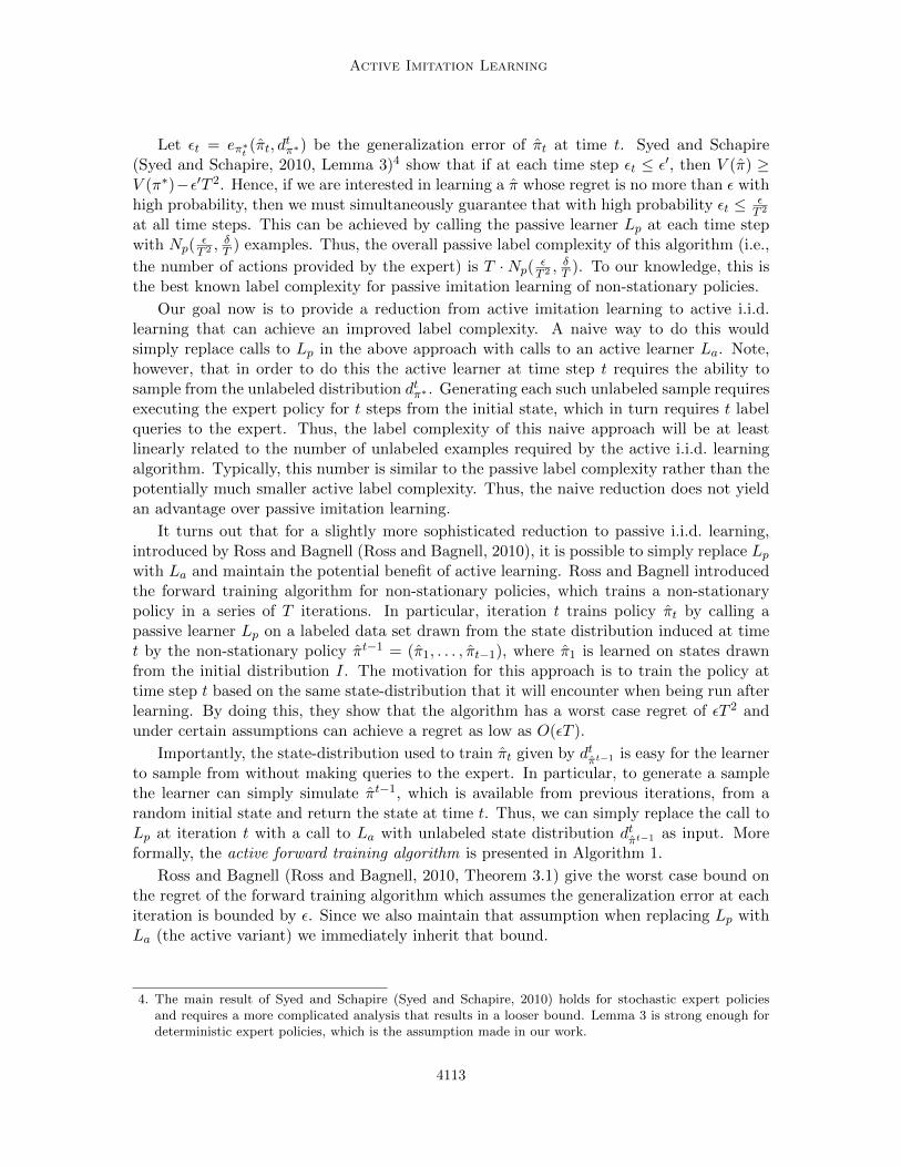
Algorithm 1 Active Forward Training
Input: active i.i.d. learning algorithm La, ε, δOutput: non-stationary policy π = (π1, . . . , πT )
1: Initialize π1 = La(ε,δT, I) . queries by La answered by expert; unlabeled data
is generated from initial state distribution I.2: for t = 2 to T do3: πt−1 = (π1, . . . , πt−1)4: πt = La(ε,
δT, dtπt−1) . queries by La answered by expert; unlabeled data is
generated using simulator and πt−1 as described in the main text.5: end for6: return π = (π1, ..., πT )
Proposition 1 Given a PAC active i.i.d. learning algorithm La, if active forward trainingis run by giving La parameters ε and δ
T at each step, then with probability at least 1− δ itwill return a non-stationary policy π such that V (π) ≥ V (π∗)− εT 2.
Note that La is run with δT as the reliability parameter to ensure that all T iterations
succeed with probability at least 1− δ.We can apply Proposition 1 to obtain the overall label complexity of active forward
training required to achieve a regret of less than ε with probability at least 1 − δ. Inparticular, we must run the active learner at each of the T iterations with parameters ε
T 2
and δT , giving an overall label complexity of
∑Tt=1Na(
εT 2 ,
δT , d
tπt−1), where d1
π0 = I and theπt−1 are random variables in this expression. Recall, from above, that the best known labelcomplexity of passive imitation learning is T ·Np(
εT 2 ,
δT ).
Comparing these quantities we see that if we use an active learning algorithm whosesample complexity is no worse than that of passive, i.e., Na(
εT 2 ,
δT , d
tπt−1) is no worse than
Np(εT 2 ,
δT ) for any t, then the expected sample complexity of active imitation learning
will be no worse than the passive case. As mentioned in the previous section, such i.i.d.active learning algorithms can be realized. Further, if in addition, for some iterations theexpected value of Na(
εT 2 ,
δT , d
tπt−1) for some values of t is better than the passive complexity,
then there will be an overall expected improvement over passive imitation learning. Whilethis additional condition cannot be verified in general, we know that such cases can exist,including cases of exponential improvement. Further, empirical experience in the i.i.d.setting also suggests that in practice Na can often be expected to be substantially smallerthan Np and rarely worse. The above result suggests that those empirical gains will be ableto transfer to the imitation learning setting.
4.2 Stationary Policies
A drawback of active forward training is that it is impractical for large T and the resultingpolicy cannot be run indefinitely. We now consider the case of learning stationary policies;first we review the existing results for passive imitation learning.
In the traditional approach, a stationary policy π is trained on the expert state distribu-tion dπ∗ using a passive learning algorithm Lp and returning a stationary policy π. Ross andBagnell (Ross and Bagnell, 2010, Theorem 2.1) show that if the generalization error of π
4114

Active Imitation Learning
Algorithm 2 RAIL
Input: active i.i.d. learning algorithm La, ε, δOutput: stationary policy π
1: Initialize π0 to arbitrary policy or based on prior knowledge2: for t = 1 to T do3: πt = La(ε,
δT, dπt−1) . queries by La answered by expert; unlabeled data is
generated using simulator as described in Section 34: end for5: return πT
with respect to the i.i.d. distribution dπ∗ is bounded by ε′ then V (π) ≥ V (π∗)− ε′T 2. Sincegenerating i.i.d. samples from dπ∗ can require up to T queries (see Section 3) the passivelabel complexity of this approach for guaranteeing a regret less than ε with probability atleast 1−δ is T ·Np(
εT 2 , δ). Again, to our knowledge, this is the best known label complexity
for passive imitation learning. Further, Ross and Bagnell (Ross and Bagnell, 2010) showthat there are imitation learning problems where this bound is tight, showing that in theworst case, the traditional approach cannot be shown to do better.
The above approach cannot be converted into an active imitation learner by simply re-placing the call to Lp with La, since again we cannot sample from the unlabeled distributiondπ∗ without querying the expert. To address this issue, we introduce a new algorithm calledRAIL (Reduction-based Active Imitation Learning) which makes a sequence of T calls toan active i.i.d. learner, noting that it is likely to find a useful stationary policy well beforeall T calls are issued. RAIL is an idealized algorithm intended for analysis, which achievesthe theoretical goals but has a number of inefficiencies from a practical perspective. Laterin Section 5, we describe the practical instantiation that is used in our experiments.
RAIL is similar in spirit to active forward training, though its analysis is quite differentand more involved. Like forward-training, RAIL iterates for T iterations, but on eachiteration, RAIL learns a new stationary policy πt that can be applied across all time stepst = 1 . . . T . Note that T denotes the length of the horizon as well as the total number ofiterations that RAIL runs for. Similarly t denotes a single time step as well as a singleiteration of RAIL. Iteration t+1 of RAIL learns a new policy πt+1 that achieves a low errorrate at predicting the expert’s actions with respect to the state distribution of the previouspolicy dπt . More formally, Algorithm 2 gives pseudocode for RAIL. The initial policy π0 isarbitrary and could be based on prior knowledge and the algorithm returns the final policyπT , which is learned using the active learning applied to unlabeled state distribution dπT−1 .
Similar to active forward training, RAIL makes a sequence of T calls to an active learner.Unlike forward training, however, the unlabeled data distributions used at each iterationcontains states from all time points within the horizon, rather than being restricted to statesarising at a particular time point. Because of this difference, the active learner is able toask queries across a range of time points and we might expect policies learned in earlieriterations to achieve non-trivial performance throughout the entire horizon. In contrast, atiteration t the policy produced by forward training is only well defined up to time t.
4115

Judah, Fern, Dietterich and Tadepalli
The complication faced by RAIL, however, compared to forward training, is that thedistribution used to train πt+1 differs from the state distribution of the expert policy dπ∗ .This is particularly true in early iterations of RAIL, since π0 is initialized arbitrarily. Intu-itively, however, we might expect that as the iterations proceed, the unlabeled distributionsused for training dπt will become similar to dπ∗ . To see this, consider the first iteration.While dπ0 need not be at all similar to dπ∗ overall, we know that they will agree on theinitial state distribution. That is, we have that d1
π0 = d1π∗ = I. Because of this, the policy
π1 learned on dπ0 can be expected to agree with the expert on the first step. This impliesthat the states encountered after the first action of the expert and learned policy will tendto be similar. That is d2
π1 will be similar to d2π∗ . In this same fashion we might expect dt+1
πt
to be similar to dt+1π∗ after iteration t. We now show that this intuition can be formalized in
order to bound the disparity between dπT and dπ∗ , which will allow us to bound the regretof the learned policy. We first state the main result, which we prove below.
Theorem 2 Given a PAC active i.i.d. learning algorithm La, if RAIL is run with parame-ters ε and δ
T passed to La at each iteration, then with probability at least 1− δ it will returna stationary policy π such that V (π) ≥ V (π∗)− εT 3.
Recall that the corresponding regret for active forward training of non-stationary policieswas εT 2. From this we see that the impact of moving from non-stationary to stationarypolicies in the worst case is a factor of T in the regret bound. Similarly the bound is afactor of T worse than the comparable result above for passive imitation learning, whichsuffered a worst-case regret of εT 2. From this we see that the total label complexity forRAIL required to guarantee a regret of ε with probability 1 − δ is
∑Tt=1Na(
εT 3 ,
δT , dπt−1)
compared to the above label complexity of passive learning T ·Np(εT 2 , δ).
We first compare these quantities in the worst case. If, in each iteration, the active i.i.d.label complexity is the same as the passive complexity, then active imitation learning viaRAIL can ask more queries than passive. That is, the active complexity would scale asT ·Np(
εT 3 ,
δT ) versus T ·Np(
εT 2 , δ), which is dominated by the factor of 1
T difference in theaccuracy parameters. In the realizable setting with finite VC-dimension, RAIL’s complexitycould be a factor of T higher than passive in this worst-case scenario.
However, if across the iterations the expected active i.i.d. label complexityNa(εT 3 ,
δT , dπt−1)
is substantially better than Np(εT 3 ,
δT ), then RAIL will leverage those savings. For exam-
ple, in the realizable setting with finite VC-dimension, if all distributions dπt−1 result in afinite disagreement coefficient, then we can get exponential savings. In particular, ignor-ing the dependence on δ (which is only logarithmic), we get an active label complexity of
O(T log T 3
ε ) versus the corresponding passive complexity of O(T3
ε ).
The above analysis points to an interesting open problem. Is there an active imitationlearning algorithm that can guarantee to never perform worse than passive, while at thesame time showing exponential improvement in the best case?
For the proof of Theorem 2, we introduce the quantity P tπ(M), which is the probabilitythat a policy π is consistent with a length t trajectory generated by the expert policy π∗ inMDP M . It will also be useful to index the state distribution of π by the MDP M , denotedby dπ(M). The main idea is to show that at iteration t, P tπt(M) is not too small, meaningthat the policy at iteration t mostly agrees with the expert for the first t actions. We first
4116

Active Imitation Learning
state two lemmas, that are useful for the final proof. First, we bound the regret of a policyin terms of P Tπ (M).
Lemma 3 For any policy π, if P Tπ (M) ≥ 1− ε, then V (π) ≥ V (π∗)− εT .
Proof Let Γ∗ and Γ be all state-action sequences of length T that are consistent with π∗
and π respectively. If R(T ) is the total reward for a sequence T then we get the following
V (π) =∑T ∈Γ
Pr(T |M,π)R(T )
≥∑
T ∈Γ∩Γ∗
Pr(T |M,π)R(T )
=∑T ∈Γ∗
Pr(T |M,π∗)R(T )−∑
T ∈Γ∗−Γ
Pr(T |M,π∗)R(T )
= V (π∗)−∑
T ∈Γ∗−Γ
Pr(T |M,π∗)R(T )
≥ V (π∗)− T ·∑
T ∈Γ∗−Γ
Pr(T |M,π∗)
≥ V (π∗)− εT.
The last two inequalities follow since the reward for a sequence must be no more than T ,and due to our assumption about P Tπ (M).
Next, we show how the value of P tπ(M) changes across one iteration of RAIL. Weshow that if we learn a policy π on state distribution dπ(M) of policy π whose error rateeπ∗(π, dπ(M)) (see Section 3.3) w.r.t. to the expert’s policy π∗ is no more than ε, thenP t+1π (M) is at least as large as P tπ(M)− Tε. When π and π correspond to policies learned
at iteration t and (t+1) respectively, then Lemma 4 describes change in the value of P tπ(M)across one iteration.
Lemma 4 For any policies π and π and 1 ≤ t < T , if eπ∗(π, dπ(M)) ≤ ε, then P t+1π (M) ≥
P tπ(M)− Tε.
Proof We define Γ to be all sequences of state-action pairs of length t+1 that are consistentwith π. Also define Γ to be all length t+ 1 state-action sequences that are consistent withπ on the first t state-action pairs (so need not be consistent on the final pair). We alsodefine M ′ to be an MDP that is identical to M , except that the transition distribution ofany state-action pair (s, a) is equal to the transition distribution of action π(s) in state s.That is, all actions taken in a state s behave like the action selected by π in s.
We start by arguing that if eπ∗(π, dπ(M)) ≤ ε then P t+1π (M ′) ≥ 1−Tε, which relates our
error assumption to the MDP M ′. To see this, note that for MDP M ′, all policies, includingπ∗, have state distribution given by dπ. Thus by the union bound 1−P t+1
π (M ′) ≤∑t+1
i=1 εi,where εi is the error of π at predicting π∗ on distribution diπ. This sum is bounded by Tε
4117

Judah, Fern, Dietterich and Tadepalli
since eπ∗(π, dπ(M)) = 1T
∑Ti=1 εi. Using this fact we can now derive the following
P t+1π (M) =
∑T ∈Γ
Pr(T |M,π∗)
≥∑T ∈Γ∩Γ
Pr(T |M,π∗)
=∑T ∈Γ
Pr(T |M,π∗)−∑T ∈Γ−Γ
Pr(T |M,π∗)
= P tπ(M)−∑T ∈Γ−Γ
Pr(T |M,π∗)
= P tπ(M)−∑T ∈Γ−Γ
Pr(T |M ′, π∗)
≥ P tπ(M)−∑T 6∈Γ
Pr(T |M ′, π∗)
≥ P tπ(M)− (1− P t+1π (M ′))
≥ P tπ(M)− Tε.
The equality of the fourth line follows because Γ contains all sequences whose first t actionsare consistent with π with all possible combinations of the remaining action and state tran-sition. Thus, summing over all such sequences yields the probability that π∗ agrees with thefirst t steps. The equality of the fifth line follows because Pr(T | M,π∗) = Pr(T | M ′, π∗)for any T that is in Γ and for which π∗ is consistent (has non-zero probability under π∗).The final line follows from the above observation that P t+1
π (M ′) ≥ 1− Tε.
We can now complete the proof of the main theorem.Proof [Proof of Theorem 2] Using failure parameter δ
T in the call to La in each iterationof RAIL ensures that with at least probability (1 − δ) that for all 1 ≤ t ≤ T , we will haveeπ∗(π
t, dπt−1(M)) ≤ ε, where dπ0(M) denotes the state distribution of the initial policy π0.This can be easily shown using the union bound. Next, we show using induction that for1 ≤ t ≤ T , we have P tπt ≥ 1− tT ε. As a base case for iteration t = 1, we have P 1
π1 ≥ 1−Tε,since the the error rate of π1 relative to the initial state distribution at time step t = 1 isat most Tε (this is the worst case when all errors are committed at time step 1). Assumethat the inequality holds for t = k, i.e., P k
πk≥ 1− kTε. Consider πk+1 trained on dπk(M).
By the union bound argument above, we know that eπ∗(πk+1, dπk(M)) ≤ ε. Hence, πk+1
and πk satisfy the precondition of Lemma 4. Therefore we have
P k+1πk+1 ≥ P kπk − Tε (by Lemma 4)
≥ 1− kTε− Tε (by inductive argument)
≥ 1− (k + 1)Tε.
Hence, for 1 ≤ t ≤ T , we have P tπt ≥ 1 − tT ε. In particular, when t = T , we haveP TπT≥ 1− T 2ε. Combining this with Lemma 3 completes the proof.
4118

Active Imitation Learning
4.3 Agnostic Case
Above we considered the realizable setting, where the expert’s policy was assumed to be ina known hypothesis class H. In the agnostic case, we do not make such an assumption. Thelearner still outputs a hypothesis from a class H, but the unknown policy is not necessarilyin H. The agnostic i.i.d. PAC learning setting is defined similarly to the realizable setting,except that rather than achieving a specified error bound of ε with high probability, a learnermust guarantee an error bound of infπ∈H ef (π,DX )+ε with high probability (where f is thetarget), where DX is the unknown data distribution. That is, the learner is able to achieveclose to the best possible accuracy given class H. In the agnostic case, it has been shownthat exponential improvement in label complexity with respect to 1
ε is achievable wheninfπ∈H ef (π,DX ) is relatively small compared to ε (Dasgupta, 2011). Further, there aremany empirical results for practical active learning algorithms that demonstrate improvedlabel complexity compared to passive learning.
It is straightforward to extend our above results for non-stationary and stationary poli-cies to the agnostic case by using agnostic PAC learners for Lp and La. Here we outlinethe extension for RAIL. Note that the RAIL algorithm will call La using a sequence ofunlabeled data distributions, where each distribution is of the form dπ for some π ∈ Hand each of which may yield a different minimum error given H. For this purpose, wedefine ε∗ = supπ∈H inf π∈H eπ∗(π, dπ) to be the minimum generalization error achievablein the worst case considering all possible state distributions dπ that RAIL might possiblyencounter. With minimal changes to the proof of Theorem 1, we can get an identical result,except that the regret is (ε∗ + ε)T 3 rather than just εT 3. A similar change in regret holdsfor passive imitation learning. This shows that in the agnostic setting we can get significantimprovements in label complexity via active imitation learning when there are significantsavings in the i.i.d. case.
5. RAIL-DA: A Practical Variant of RAIL
Despite the theoretical guarantees, there are at least two potential drawbacks of the RAILalgorithm from a practical perspective. First, RAIL does not share labeled data acrossiterations which is potentially wasteful in practice, though important for our analysis. Inpractice, we might expect that aggregating labeled data across iterations would be beneficialdue to the larger amount of data. This is somewhat confirmed by the empirical successof the DAGGER algorithm (Ross et al., 2011) and motivates evaluating the use of dataaggregation within RAIL. Incorporating data aggregation into RAIL, however, complicatesthe theoretical analysis, which we leave for future work. The second practical inefficiency ofRAIL is that the unlabeled state distributions used at early iterations may be quite differentfrom dπ∗ . In particular, the state distribution of policy πt, which is used to train the policyat iteration t + 1, is only guaranteed to be close to the expert’s state distribution for thefirst t time steps and can (in the worst case) differ arbitrarily at later times. Thus, earlyiterations may focus substantial query effort on parts of the state space that are not themost relevant for learning π∗.
4119
Judah, Fern, Dietterich and Tadepalli
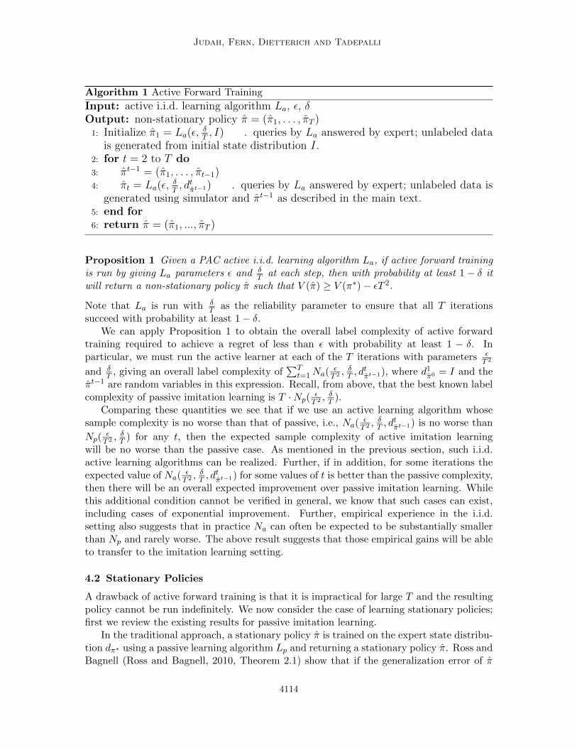
Algorithm 3 RAIL+
Input: L0, n, AccumData, N , K. L0 : initial set of labeled data. n : no. of queries per iteration. AccumData : accumulate data across iterations or not. N : committee size for DWQBC. K : # trajectories used to generate unlabeled data
Output: stationary policy π
1: Initialize L = L0
2: while query budget remaining do3: U = SampleUnlabeledData(K,L) . generates pool of unlabeled data4: if !AccumData then5: Initialize L = L0
6: end if7: for i = 1 to n do . select n queries from pool U8: s = DWQBC(L,U ,N) . density-weighted QBC is used as active i.i.d. learner9: L = L ∪ {(s, Label(s))} . obtain label from expert
10: end for11: end while12: return π = SupervisedLearn(L)
We now describe a parameterized practical instantiation of RAIL used in our experi-ments, which is intended to address the above issues and also specify certain other imple-mentation details. Algorithm 3 gives pseudocode for this algorithm, which we call RAIL+
to distinguish it from the idealized version of RAIL in our analysis. In Section 6, we willcompare different instances of RAIL+, including parameterizations corresponding to pureRAIL and RAIL-DA (for data aggregation), which is the primary algorithm in our empiricalstudy. We note that our description assumes the use of a pool-based active learner, whichis a common active learning setting, meaning that the learner requires as input a pool ofunlabeled examples U that represents the unlabeled target distribution.
5.1 Data Aggregation and Incremental Querying
The first major difference compared to RAIL is that RAIL+ can aggregate data acrossiterations when the Boolean parameter AccumData is set to true. In this case, duringeach iteration the newly labeled data is added to the set of labeled data from previousiterations (lines 7-10). Otherwise, the labeled data from previous iterations is discardedafter generating unlabeled data U (lines 4-6).
The second major difference is that RAIL+ may ask fewer queries per iteration thanRAIL as specified by the parameter n. RAIL corresponds to a version of RAIL+ thatdoes not use data aggregation and has n = Na. Because RAIL+ can aggregates data, itopens up the possibility of asking only a small number of queries per iteration (n � Na)and hence behaving more incrementally. This is reflected in the main loop of Algorithm 3
4120

Active Imitation Learning
Algorithm 4 Density-Weighted Query-By-Committee Algorithm
1: procedure DWQBC(L,U ,N)2: C = SampleCommittee(N ,L) . committee represents posterior over policies3: dL =EstimateDensity(U) . estimate density of states in U (see text)4: s∗ = argmax{V E(s, C) ∗ dL(s) : s ∈ U} . selection heuristic (see text)5: return s∗
6: end procedure
(lines 2-11). Each iteration starts with the current set of labeled examples L, which havebeen accumulated across all previous iterations by RAIL+. This set of examples is used togenerate a pool U of unlabeled examples/states (see details below) intended to representthe unlabeled target distribution. A pool-based active learner, DWQBC (explained later),is then called n times to select n queries from this pool. Each query is labeled by the expertand added to the growing set of labeled training data L. After the n queries have beenissued and L is updated, the next iteration begins.
This incremental version of RAIL allows for rapid updating of the unlabeled state dis-tributions used for learning (represented via U) and prevents RAIL from using its querybudget on earlier less accurate distributions. In our experiments, we find that using n = 1is most effective compared to larger values, which facilitates the most rapid update of thedistribution. In this case, each query selected by the active i.i.d. learner is based on themost up-to-date state distribution, which takes all prior data into account. We refer to thisbest performing variant of RAIL+ with n = 1 and data aggregation as RAIL-DA.
An interesting variation to RAIL+ is when queries take a non-trivial amount of real-timeto answer and there are k experts available that can answer queries in parallel. In this case,it can be beneficial to ask k simultaneous queries per iteration in order to reduce the amountof real-time required to learn a policy. The problem of selecting k such queries is known asbatch active learning, and a variety of approaches are available for the i.i.d. setting (Brinker,2003; Xu et al., 2007; Hoi et al., 2006a,b; Guo and Schuurmans, 2008; Azimi et al., 2012).An advantage of our reduction-based approach to active imitation learning is that we candirectly plug in the i.i.d. batch active learner in our framework without requiring any otherchanges to be made.
5.2 Density Weighted QBC
Since it is important that the active i.i.d. learner be sensitive to the unlabeled data dis-tribution, we choose a density-weighted learning algorithm. In particular, we use density-weighted query-by-committee (McCallum and Nigam, 1998) in our implementation. Givena set of labeled data L and unlabeled data U , this approach first uses bootstrap aggregationon L in order to generate a policy committee for query selection (Algorithm 4, line 2). Inour experiments we use a committee of size 5. The approach then computes a density esti-mator over the unlabeled data U (line 3). In our implementation we use a simple distancebased binning approach to density estimation, though more complex approaches could beused. The selected query is the state that maximizes the product of state density andcommittee disagreement (line 4). As a measure of disagreement we use the entropy of thevote distribution (Dagan and Engelson, 1995) (denoted as VE), which is a common choice.
4121
Judah, Fern, Dietterich and Tadepalli
Algorithm 5 Procedure SampleUnlabeledData
1: procedure SampleUnlabeledData(K,L)2: C = SampleCommittee(K,L) . committee represents posterior over policies3: U = {} . initialize multi-set of unlabeled data4: for π ∈ C do5: S = SimulateTrajectory(π) . states generated on trajectory of π6: U = U ∪ S7: end for8: return U9: end procedure
Intuitively, the selection heuristic of DWQBC attempts to trade off the uncertainty aboutwhat to do at a state (measured by VE) with the likelihood that the state is relevant tolearning the target policy (measured by the density).
5.3 Bayesian Learner
The final choice we make while implementing RAIL+ (and hence RAIL-DA) is again mo-tivated by the goal of arriving at an accurate unlabeled data distribution as quickly aspossible. Recall that at iteration t + 1, RAIL learns using an unlabeled data distributiondπt , where πt is a point estimate of the policy based on the labeled data from iteration t.In order to help improve the accuracy of this unlabeled distribution (with respect to dπ∗),instead of using a point estimate, we adopt a Bayesian approach in RAIL+. In particular,at iteration t let L be the set of state-action pairs collected from the previous iteration(or from all previous iterations if data is accumulated). We use this to define a posteriorP (π|L) over policies in our policy class H. This distribution, in turn, defines a posteriorunlabeled state distribution dL = Eπ∼P (π|L)[dπ(s)] that RAIL+ effectively uses in place ofdπt as used in RAIL. Note that we can sample states from dL by first sampling a policy πand then sampling a state from dπ, all of which can be done without interaction with theexpert.
Our implementation of this idea uses bootstrap aggregation (Breiman, 1996) in orderto approximate dL by an unlabeled data pool U via a call to the procedure Sample-UnlabeledData in Algorithm 3 (line 3). Our implementation assumes a class of linearparametric policies with a zero-mean Gaussian prior over the parameters. The procedurefirst uses bootstrap aggregation to approximate sampling a set of policies from the posterior(Algorithm 5, line 2) forming a “committee” C of K policies. We view C as an empiricaldistribution representing the posterior over policies. In particular, each policy is the resultof first generating a bootstrap sample of the current labeled data and then calling a super-vised learner on the sampled data. Each member of the committee is then simulated toform a state trajectory, and the states on those trajectories are aggregated to produce theunlabeled data pool U (Algorithm 5, lines 4-7). Our implementation uses K = 5.
From a theoretical perspective, the use of a Bayesian classifier does not impact thevalidity of RAIL’s performance guarantee provided that the Bayesian approach providesPAC guarantees. In fact, early theoretical work in active learning (Freund et al., 1997) usedexactly this type of assumption in their analysis of the query-by-committee algorithm.
4122

Active Imitation Learning
Algorithm 6 Procedure SampleCommittee
1: procedure SampleCommittee(K,L)2: C = {} . initialize the committee3: for i = 1 to K do4: L′ = BootstrapSample(L) . create a bootstrap sample of L5: π′ = SupervisedLearn(L′) . learn a classifier(policy) using L′
6: C = C ∪ π′7: end for8: return C9: end procedure
In practice, dL is a significantly more useful estimate of dπ∗ than the point estimatewith respect to learning a policy. This is because it places more weight on states that aremore frequently visited by policies drawn from the posterior rather than just a single policy.As an extreme example of the advantage of using dL in practice, consider active imitationlearning in an MDP with deterministic dynamics and a single start state. At iteration t,RAIL will use the state distribution of the point estimate πt−1, which for our assumedMDP will be uniform over the deterministic state sequence generated by πt−1. Thus, activelearning will place equal emphasis on learning among that set of states. This is despite thefact that, in early iterations, we should expect that states appearing later in the trajectoryare less likely to be relevant to learning π∗. This is because inaccuracies in πt−1 lead toerror propagation as the trajectory unfolds. In contrast, dL will weigh states according tothe trajectories produced by all policies, weighted by the posterior. The practical effect isa non-uniform distribution over states in those trajectories, roughly weighted by how manypolicies visit the states. Thus, states at the tail end of trajectories in early iterations willgenerally carry very little weight, since they are only visited by one or a small number ofpolicies.
6. Experiments
We conduct our empirical evaluation on five domains: 1) Cart-pole, 2) Bicycle, 3) Wargus,4) Driving, and 5) NETtalk. Below we first describe the details of these domains. We thenpresent various experiments that we performed in these domains. In the first experiment,we study the impact of data aggregation and query size on the performance of RAIL+ fromAlgorithm 3. For this we compare several parameter settings, varying from versions thatare close to pure RAIL to RAIL-DA (n = 1 with data aggregation). We show that versionscloser to RAIL-DA that aggregate data and ask queries incrementally are more effective inpractice. In particular, we show that RAIL-DA (which aggregates data and asks only onequery per iteration) is the most effective parameterization. Next, we evaluate the impact ofanother implementation choice discussed in Section 5, the choice of base active learner inRAIL+. We show that a density-weighted base active learner leads to better performancein practice than using other base active learners that ignore the data distribution. Oncewe have shown that RAIL-DA with a density-weighted base active learner is the best, we
4123

Judah, Fern, Dietterich and Tadepalli
compare it with a number of baseline approaches to active imitation learning in our last setof experiments. Finally, we provide some overall observations.
For all the learners in the experiments that are presented in this section, we employedthe SimpleLogistic classifier from Weka (Hall et al., 2009) to learn policies over the set offeatures that were provided for each domain.
6.1 Domain Details
In this subsection, we give the details of all the domains used in our experiments.
6.1.1 Cart-Pole
Cart-pole is a well-known RL benchmark. In this domain, there is a cart on which restsa vertical pole. The objective is to keep the attached pole balanced by applying left orright force to the cart. An episode ends when either the pole falls or the cart goes out ofbounds. There are two actions, left and right, and four state variables (x, x, θ, θ) describingthe position and velocity of the cart and the angle and angular velocity of the pole. Wemade slight modifications to the usual setting where we allow the pole to fall down andbecome horizontal and the cart to go out of bounds (we used [-2.4, 2.4] as the in boundsregion). We let each episode run for a fixed length of 5000 time steps. This opens up thepossibility of generating several “undesirable” states where either the pole has fallen or thecart is out of bounds that are rarely or never generated by the expert’s state distribution.
For all the experiments in cart-pole, the learner’s policy is represented via a linearlogistic regression classifier using features of state-action pairs where features correspondto state variables. The expert policy was a hand-coded policy that can balance the poleindefinitely. For each learner, we ran experiments from 150 random initial states close tothe equilibrium start state ((x, x, θ, θ) = (0.0, 0.0, 0.0, 0.0)). For each start state a policy islearned and a learning curve is generated measuring the performance as function of numberof queries posed to the expert. To measure performance, we use a reward function (unknownto the learner) that gives +1 reward for each time step where the pole is kept balanced andthe cart is within bounds and −1 otherwise. The final learning curve is the average of theindividual curves.
6.1.2 Bicycle Balancing
This domain is a variant of the RL benchmark of bicycle balancing and riding (Randløv andAlstrøm, 1998). The goal is to balance a bicycle moving at a constant speed for 1000 timesteps. If the bicycle falls, it remains fallen for the rest of the episode. Similar to the cart-poledomain, in bicycle balancing there is a huge possibility of spending significant amount oftime in “undesirable” states where the bicycle has fallen down. The state space is describedusing nine variables (ω, ω, θ, θ, ψ, xf , yf , xb, yb), where ω and ω are the vertical angle andangular velocity of the bicycle, θ and θ are the angle and angular velocity of the handlebar, ψis the angle of the bicycle to the goal, xf and yf are x and y coordinates of the front tire andxb and yb are x and y coordinates of the rear tire of the bicycle. There are five possible actionsA = {(τ = 0, v = −0.02), (τ = 0, v = 0), (τ = 0, v = 0.02), (τ = 2, v = 0), (τ = −2, v = 0)},where the first component is the torque applied to the handlebar and the second is thedisplacement of the rider.
4124

Active Imitation Learning
As in the cart-pole domain, for all experiments in bicycle balancing, the learner’s policyis represented as a linear logistic regression classifier over features of state-action pairs. Afeature vector for a state-action pair is defined as follows: Given a state s, a vector consistingof following 20 basis functions is computed:
(1, ω, ω, ω2, ω2, ωω, θ, θ, θ2, θ2, θθ, ωθ, ωθ2, ω2θ, ψ, ψ2, ψθ, ψ, ψ2, ψθ)T ,
where ψ = π − ψ if ψ > 0 and ψ = −π − ψ if ψ < 0. This vector of basis functions isrepeated for each of the 5 actions giving a feature vector of length 100. The expert policywas hand-coded and can balance the bicycle for up to 26K time steps. We used a similarevaluation procedure as for cart-pole where we generated 150 random start states and foreach start state, a policy was learned using each of the learning algorithms and a learningcurve was generated measuring total reward as function of number of queries posed to theexpert. We give a +1 reward for each time step where the bicycle is kept balanced and a−1 reward otherwise.
6.1.3 Wargus
We consider controlling a group of 5 friendly close-range military units against a group of5 enemy units in the real-time strategy game Wargus, similar to the setup used by Judahet al. (Judah et al., 2010). The objective is to win the battle while minimizing the lossin total health of friendly units. The set of actions available to each friendly unit is toattack any one of the remaining units present in the battle (including other friendly units,which is always a bad choice). In our setup, we allow the learner to control one of the unitsthroughout the battle, whereas the other friendly units are controlled by a fixed “reasonablygood” policy. This situation would arise when training the group via coordinate ascent onthe performance of individual units. The expert policy corresponds to the same policy usedby the other units. Note that poor behavior from even a single unit generally results in ahuge loss.
The learner’s policy is represented using 27 state-action features that capture differentinformation about the current battle situation such as the distance between the friendlyagent and the target of attack, whether the target is already under attack by other friendlyunits, health of the target relative to friendly unit, whether the target is actually a friendlyunit, etc. Providing full demonstrations in real time in such tactical battles is very difficultfor human players and quite time consuming if demonstrations are done in slow motion,which motivates state-based active learning for this domain. For experiments, we designed21 battle maps differing in the initial unit positions, using 5 for training and 16 for testing.We report results in the form of learning curves showing the performance metric as afunction of number of queries posed to the expert. We use the difference in the total healthof friendly and enemy units at the end of the battle as the performance metric (whichis positive for a win). Due to the slow pace of the experiments running on the Wargusinfrastructure, we average results across at most 20 trials.
6.1.4 Driving Domain
The driving domain is a traffic navigation problem often used as a test domain in theimitation learning literature (Abbeel and Ng, 2004). This domain was also the main test
4125

Judah, Fern, Dietterich and Tadepalli
Figure 1: Screenshot of the driving simulator.
bed used to evaluate the confidence based autonomy (CBA) learner in prior work (Chernovaand Veloso, 2009). Here we evaluate RAIL-DA on a particular implementation of the drivingdomain used by Cohn et al. (Cohn et al., 2011). In this domain, the goal is to successfullynavigate a car through traffic on a busy five lane highway. The highway consists of threetraffic lanes and two shoulder lanes (see Figure 1). The learner controls the black car, whichmoves at a constant speed. The other cars move at a randomly chosen continuous-valuedconstant speed, and they don’t change lanes. At each discrete time step, the learner controlsthe car by taking one of the three actions: 1) Left, which moves the car to the adjacent leftlane, 2) Right, which moves the car to the adjacent right lane, and 3) Stay, which keeps thecar in the current lane. The agent is allowed to drive on the shoulder lane but cannot moveoff the shoulder lanes.
The learner’s policy is represented as a linear logistic regression classifier that maps agiven state to one of the three actions. The state space is represented using 68 features. Thefirst 5 features are binary features that specify the learner’s current lane. The next 3 binaryfeatures specify whether the learner is colliding with, tailgating or trailing another car. Theremaining 60 features, consisting of three parts, one for the learner’s current lane and twofor the two adjacent lanes, which are binary features that specify whether the learner’s carwill collide with or pass another car in 2X time steps, where X ranges from 0 to 19. Thiscaptures the agent’s view of the traffic while taking car velocities into account.
To conduct experiments in the driving domain, we carefully designed a reward functionthat induces good driving behavior and used Sarsa(λ) (Sutton and Barto, 1998) with linearfunction approximation to learn a policy to serve as the expert policy. The expert policyuses the same set of 68 features as used by the agent for value function approximation.For each learner, we ran 100 different learning trials where during each trial the learner isallowed to pose a maximum of 500 (1000 in Experiment 1) queries to the expert and learnfrom it. For each trial, a learning curve is generated that measures the performance as afunction of the number of queries posed to the expert. To measure performance, after eachquery is posed and the policy is updated, the updated policy is allowed to navigate the carfor 1000 time steps in a test episode, and the total reward is recorded. The final performancemeasure is the average total reward per episode measured over 500 test episodes. The finallearning curve is the average over all 100 trials.
4126

Active Imitation Learning
6.1.5 Structured Prediction
We evaluate RAIL-DA on two structured prediction tasks, stress prediction and phonemeprediction, both based on the NETtalk data set (Dietterich et al., 2008). In stress prediction,given a word, the goal is to assign one of the 5 stress labels to each letter of the word in left-to-right order so that the word is pronounced correctly. The output labels are ‘2’ (strongstress), ‘1’ (medium stress), ‘0’ (light stress), ‘<’ (unstressed consonant, center of syllableto the left), and ‘>’ (unstressed consonant, center of syllable to the right). In phonemeprediction, the task is to assign one of the 51 phoneme labels to each letter of the word. Itis straightforward to view structured prediction as imitation learning (see for example Rosset al., 2011,Daume et al., 2009) where at each time step (letter location), the learner hasto execute the correct action (i.e., predict correct label) given the current state. The stateconsists of features describing the input (the current letter and its immediate neighbors) andthe previous L predictions made by the learner (the prediction context). In our experiments,we use L = 1, 2.
The NETtalk data set consists of 2000 words divided into 1000 training words and1000 test words. Each method is allowed to select a state located on any of the wordsin the training data and pose it as a query. The expert reveals the correct label at thatlocation. We use character accuracy as a measure of performance. The details of how ineach learning trial RAIL-DA and other baselines select a query from the set of trainingwords will be described when we present our results in the following subsections. We reportfinal performance in the form of learning curves averaged across 50 learning trials.
6.2 Experiment 1: Evaluation of the Effects of Data Aggregation and QuerySize
We compare different versions of RAIL+, by varying the parameters AccumData and n inAlgorithm 3, in order to observe the impact of data aggregation and query size. We use thenotation RAIL+-n-DA for versions that aggregate data and ask n queries per iteration anduse RAIL+-n to denote variants that ask n queries per iteration without data aggregation.Note that RAIL+-1-DA is the same as RAIL-DA and that RAIL+-n with a large value of ncorresponds to the original version of RAIL from our analysis. Note that all these variantsuse the DWQBC active i.i.d. learner as described in Section 5.
For this experiment, we focus on three domains: 1) Cart-Pole, 2) Bicycle Balancing, and3) Driving Domain. In each domain, we evaluated RAIL+-n-DA and RAIL+-n for valuesof n starting at n = 1 in increments until some maximum value. The maximum value of nin each domain was selected to be a value where i.i.d. active learning from the true expertstate distribution reliably converged to a near perfect policy. For each RAIL+ variant anddomain, we show the averaged learning curve as described earlier.
Figure 2 shows the results of the experiment. We first discuss results in the Bicycledomain due to more discernible trends in this domain. Figure 2(b) shows results of theexperiment in the Bicycle domain. First, observe the impact of data aggregation by com-paring each pair RAIL+-n and RAIL+-n-DA. Clearly, RAIL+-n-DA is significantly betterthan RAIL+-n for each value of n, indicating that it is generally better to aggregate dataacross iterations in this domain. This is likely explained by the fact that the use of ag-gregation allows for the algorithms to learn from more data at later iterations. This is
4127

Judah, Fern, Dietterich and Tadepalli
0 100 200 300 400 500 600 700 800 900 1000−4000
−3000
−2000
−1000
0
1000
2000
3000
4000
5000
6000
Number of Queries
To
tal
Re
wa
rd
Expert
RAIL+−50
RAIL+−50−DA
RAIL+−10
RAIL+−10−DA
RAIL+−1
RAIL+−1−DA (RAIL−DA)
(a)
0 50 100 150 200 250 300 350 400 450 5000
100
200
300
400
500
600
700
800
900
1000
Number of Queries
To
tal R
ew
ard
Expert
RAIL+−100
RAIL+−100−DA
RAIL+−50
RAIL+−50−DA
RAIL+−10
RAIL+−10−DA
RAIL+−1
RAIL+−1−DA (RAIL−DA)
(b)
0 100 200 300 400 500 600 700 800 900 1000−5
−4
−3
−2
−1
0
1x 10
4
Number of Queries
To
tal R
ew
ard
Expert
RAIL+−200
RAIL+−200−DA
RAIL+−100
RAIL+−100−DA
RAIL+−50
RAIL+−50−DA
RAIL+−1
RAIL+−1−DA (RAIL−DA)
(c)
Figure 2: Evaluation of the effects of data aggregation and query size in RAIL+: (a) Cart-pole (b) Bicycle balancing (c) Driving domain.
4128

Active Imitation Learning
particularly important for small values of n, such as n = 1 and n = 10, where withoutaggregation each iteration is learning from only a small amount of data (the small amountof initial data + n).
Now consider the impact of varying n with the use of aggregation in Bicycle. Theclear trend is that when aggregation is being used the performance improves significantlyas n decreases from n = 100 to n = 1. That is, the more incremental variants of RAIL+
dominate, with n = 1 (i.e. the RAIL-DA algorithm) dominating all others by a large margin.The main reason for this particularly striking trend is that in Bicycle the distributions beinglearned from in early iterations are quite distant from that of the expert. In particular, theearly iterations involve learning from state distributions of policies that result in earlycrashes, and hence many useless states from the point of view of learning. This means thatwhen using n = 100, the first 100 queries are selected from such a distribution and notmuch is learned. In fact, we see a downward trend, indicating that learning from thosedistributions hurts performance. On the other hand, as n decreases fewer queries are spenton those early inaccurate distributions, and the data from a small number of queries periteration accumulates, resulting in policies that have better state distributions to learnfrom. Indeed, for n = 1, only one query is asked for each distribution, and we see very rapidimprovement until reaching expert performance after just over 50 queries.
Figure 2(a) shows results for Cart-Pole. The target concept in this domain is simpler,and hence the learning curves improve more quickly compared to Bicycle. However, wesee the same general trends as for Bicycle. Aggregation is beneficial and we get the bestperformance for small values of n when using aggregation. Again we see that RAIL+-1-DA(i.e., RAIL-DA) is the top performer. These same trends are observed in Figure 2(c) forDriving.
Overall, these experiments provide strong evidence that in practice aggregation is animportant enhancement to RAIL+ over RAIL, and that more incremental variants arepreferable. Thus, for the remainder of the paper we will use the RAIL-DA algorithm whichuses aggregation and n = 1.
6.3 Experiment 2: Evaluation of RAIL-DA with Different Base ActiveLearners
In Section 5, we mentioned that it is important that the active i.i.d. learner used withRAIL be sensitive to the unlabeled data distribution. To test this hypothesis, we conductedexperiments to study the effects of using active i.i.d. learners that take data distribution intoconsideration against active learners that ignore the data distribution altogether in RAIL-DA. We compare the performance of three different versions of RAIL-DA: 1) RAIL-DA, theRAIL-DA algorithm from the previous experiment that uses density-weighted QBC as thebase active learner, 2) RAIL-DA-QBC, RAIL-DA but with density-weighted QBC replacedwith the standard QBC (without density weighting), and 3) RAIL-DA-RAND, which usesrandom selection of unlabeled data points.
Figure 3 shows the performance of the three versions of RAIL-DA on our first four testdomains. We see that, in Cart-Pole, Bicycle and Wargus, RAIL-DA performs better thanboth RAIL-DA-QBC and RAIL-DA-RAND. This shows that it is critical for the activei.i.d. learner to exploit the state density information that is estimated by RAIL-DA at
4129

Judah, Fern, Dietterich and Tadepalli
0 10 20 30 40 50 60 70 80 90 100−4000
−3000
−2000
−1000
0
1000
2000
3000
4000
5000
6000
Number of Queries
To
tal
Re
wa
rd
Expert
RAIL−DA
RAIL−DA−QBC
RAIL−DA−RAND
(a)
0 10 20 30 40 50 60 70 80 90 100−200
0
200
400
600
800
1000
1200
Number of Queries
To
tal R
ew
ard
Expert
RAIL−DA
RAIL−DA−QBC
RAIL−DA−RAND
(b)
0 10 20 30 40 50 60 70 80 90 100−20
0
20
40
60
80
100
120
140
Number of Queries
To
tal R
ew
ard
Expert
RAIL−DA
RAIL−DA−QBC
RAIL−DA−RAND
(c)
0 50 100 150 200 250 300 350 400 450 500−5
−4
−3
−2
−1
0
1x 10
4
Number of Queries
To
tal R
ew
ard
Expert
RAIL−DA
RAIL−DA−QBC
RAIL−DA−RAND
(d)
Figure 3: Performance of RAIL-DA with different base active learners on (a) Cart-pole (b)Bicycle balancing (c) Wargus (d) Driving Domain.
4130

Active Imitation Learning
0 50 100 150 200 250 3000.35
0.4
0.45
0.5
0.55
0.6
0.65
0.7
0.75
Number of Queries
Pre
dic
tio
n A
cc
ura
cy
pe
r C
ha
rac
ter
RAIL−DA
RAIL−DA−QBC
RAIL−DA−RAND
(a)
0 50 100 150 200 250 3000.35
0.4
0.45
0.5
0.55
0.6
0.65
0.7
0.75
Number of Queries
Pre
dic
tio
n A
cc
ura
cy
pe
r C
ha
rac
ter
RAIL−DA
RAIL−DA−QBC
RAIL−DA−RAND
(b)
0 50 100 150 200 250 3000.1
0.2
0.3
0.4
0.5
0.6
0.7
0.8
Number of Queries
Pre
dic
tio
n A
cc
ura
cy
pe
r C
ha
rac
ter
RAIL−DA
RAIL−DA−QBC
RAIL−DA−RAND
(c)
0 50 100 150 200 250 3000.1
0.2
0.3
0.4
0.5
0.6
0.7
0.8
Number of Queries
Pre
dic
tio
n A
cc
ura
cy
pe
r C
ha
rac
ter
RAIL−DA
RAIL−DA−QBC
RAIL−DA−RAND
(d)
Figure 4: Performance of RAIL-DA with different base active learners on NETtalk: (a)Stress prediction, L = 1 (b) Stress prediction, L = 2 (c) Phoneme prediction,L = 1 (d) Phoneme prediction, L = 2. Character accuracy of the expert is 1.
4131

Judah, Fern, Dietterich and Tadepalli
each iteration. Recall that in these domains, especially during early iterations, RAIL-DA is quite likely to generate several uninformative states that are far from the expert’sstate distribution (states with fallen pole or bike, or states where the friendly team isheavily outnumbered by the enemy team in Wargus). Taking state density information intoaccount helps to avoid querying in such states compared to a learner that ignores densityinformation. In the driving domain, we see that although RAIL-DA performs better thanRAIL-DA-RAND, its performance is comparable to that of RAIL-DA-QBC. This is becausein the driving domain, even states that are not close to the expert’s state distribution provideinformative training information. This allows RAIL-DA-QBC to pose useful queries andgeneralize well from them.
Figure 4 shows the performance of the three versions of RAIL-DA on the NETtalk dataset along with 95% confidence intervals. RAIL-DA and RAIL-DA-QBC can select the bestquery across the entire training set. RAIL-DA-RAND selects a random query from theset of unlabeled states generated on a random training sequence. For stress prediction, wesee that RAIL-DA performs better than both RAIL-DA-QBC and RAIL-DA-RAND. Forphoneme prediction, RAIL-DA performs better than RAIL-DA-RAND, but its performanceis comparable to RAIL-DA-QBC. Overall, we see that RAIL-DA performs best, so it willbe compared against the other baselines in the next section.
6.4 Experiment 3: Comparison of RAIL-DA with Baselines
We compare RAIL-DA against the following baselines:
1. Passive. This baseline simulates the traditional approach by starting at the initialstate and querying the expert about what to do at each visited state.
2. unif-QBC. This baseline views all the MDP states as i.i.d. according to the uniformdistribution and applies the standard query-by-committee (QBC) (Seung et al., 1992)active learning approach. Intuitively, this approach will select the state with highestaction uncertainty according to the current data set and ignores the state distribution.
3. unif-RAND. This baseline selects states to query uniformly at random.
4. Confidence based autonomy (CBA) (Chernova and Veloso, 2009). This approach re-quires the use of policies that provide some form of confidence estimate (e.g., prob-abilities over actions). Given the current set of labeled data, the approach executestrajectories of the current policy until it reaches a state where the policy confidencefalls below a threshold. It then queries the expert for the correct action and updatesthe policy accordingly. It then executes the correct action and continues until thenext low confidence state is reach. It is possible for CBA to stop asking queries oncethe confidence exceeds the threshold in all states visited by the current policy. We usethe same automated threshold adjustment strategy proposed by Chernova and Veloso(Chernova and Veloso, 2009). We also experimented with other threshold adjustmentmechanisms as well as fixed thresholds, but were unable to find an improvement thatperformed better across our domains.
Figure 5 shows the results of this experiment along with 95% confidence intervals onour first four test domains. Figure 5(a) shows the performance of RAIL-DA on cart-pole.
4132
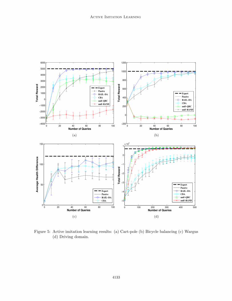
Active Imitation Learning
0 20 40 60 80 100−4000
−3000
−2000
−1000
0
1000
2000
3000
4000
5000
6000
Number of Queries
To
tal
Re
wa
rd
Expert
Passive
RAIL−DA
CBA
unif−QBC
unif−RAND
(a)
0 20 40 60 80 100−200
0
200
400
600
800
1000
1200
Number of Queries
To
tal
Re
wa
rd
Expert
Passive
RAIL−DA
CBA
unif−QBC
unif−RAND
(b)
0 20 40 60 80 1000
50
100
150
Number of Queries
Av
era
ge
He
alt
h D
iffe
ren
ce
Expert
Passive
RAIL−DA
CBA
(c)
0 100 200 300 400 500
−5
−4
−3
−2
−1
0
1x 10
4
Number of Queries
To
tal R
ew
ard
Expert
Passive
RAIL−DA
CBA
unif−QBC
unif−RAND
(d)
Figure 5: Active imitation learning results: (a) Cart-pole (b) Bicycle balancing (c) Wargus(d) Driving domain.
4133

Judah, Fern, Dietterich and Tadepalli
−12 −10 −8 −6 −4 −2 0 2 4 6
x 10−3
−0.4
−0.3
−0.2
−0.1
0
0.1
0.2
theta
the
tad
ot
(a)
−12 −10 −8 −6 −4 −2 0 2 4 6
x 10−3
−0.4
−0.3
−0.2
−0.1
0
0.1
0.2
theta
th
etad
ot
(b)
Figure 6: Queried states in Cart-pole for learners: (a) Passive, (b) RAIL-DA. The blackcircles represent states where the right action is suggested by the expert policy.The red stars represent states where the left action is suggested. The decisionboundary separating these two sets of states is a line very close to θ = 0. We seethat unlike Passive, RAIL-DA focuses its queries around the decision boundary.This figure is best viewed in color.
4134

Active Imitation Learning
We observe that RAIL-DA learns quickly and achieves optimal performance with only 30-35 queries. Passive, on the other hand, takes 100 queries to get close to the optimalperformance. The reason for this difference is clear when one visualizes the states queriedby RAIL-DA versus Passive. Figure 6(a) shows the states queried by Passive. The blackcircles represent states where the right action is suggested by the expert. The red starsrepresent states where the left action is optimal according to the expert. The decisionboundary of the expert policy is the line separating these two sets of states (very closeto θ = 0). We notice that Passive asks many uninformative queries that are not close tothe decision boundary. Figure 6(b) shows the queries posed by RAIL-DA. We see that thequeries posed by RAIL-DA tend to be close to the decision boundary of the expert policy.
A naive reduction to active learning can be dangerous, as demonstrated by the poorperformance of unif-QBC. Further, RAIL-DA performs much better than random queryselection as demonstrated by the performance of unif-RAND. By ignoring the real datadistribution altogether and incorrectly assuming it to be uniform, these naive methods endup asking many queries that are not relevant to learning the expert policy (e.g., stateswhere the pole is in an irrecoverable fall or the cart is out of bounds). CBA, like RAIL-DA,learns quickly but settles at a suboptimal level of performance. This is because it becomesconfident prematurely and stops asking queries. This shows that CBA’s automatic thresholdadjustment mechanism did not work well in this domain. We did experiment with severalmodifications to the threshold adjustment strategy, but we were unable to find one thatwas robust across all our domains. Thus we report results for the original strategy.
Figure 5(b) compares each approach in the bicycle domain. The results are similarto those of cart-pole with RAIL-DA being the top performer. Unif-RAND and Unif-QBCshow notably poor performance in this domain. This is because bicycle balancing is a harderlearning problem than cart-pole with many more uninformative states (an unrecoverablefall or fallen state). We found that almost all queries posed by Unif-RAND and Unif-QBCwere in these states. CBA does only slightly better than Passive, though unlike cart-pole,it achieves near-optimal asymptotic performance.
The results in the Wargus domain are shown in Figure 5(c). Passive learns along theexpert’s trajectory in each map on all 5 training maps considered sequentially according toa random ordering. For RAIL-DA, in each iteration a training map is selected randomlyand a query is posed in the chosen map. For CBA, a map is selected randomly and CBA isallowed to play an episode in it, pausing and querying as and when needed. If the episodeends, another map is chosen randomly and CBA continues to learn in it. After each query,the learned policy is tested on the 16 test maps. We use the difference in the total healthof friendly and enemy units at the end of the battle as the performance metric (which ispositive for a win). We did not run experiments for unif-QBC and unif-RAND, because itis difficult to define the space of feasible states over which to sample uniformly.
We see that although Passive learns quickly for the first 20 queries, it fails to improvefurther. This shows that the states located in this initial prefix of the expert’s trajectoryare very useful, but thereafter Passive gets stuck on the uninformative part of the trajec-tory until its query budget is over. On the other hand, RAIL-DA and CBA continue toimprove beyond Passive, with the performance of CBA being comparable to RAIL-DA inthis domain, which indicates that both these active learners are able to locate and querymore informative states.
4135

Judah, Fern, Dietterich and Tadepalli
The results for the driving domain are shown in Figure 5(d). We see qualitativelysimilar performance trends as in the previous three domains with RAIL-DA still being thebest performing learner and outperforming most of the competing baselines. The exceptionhowever is that unif-QBC and unif-RAND perform quite well in this domain, both beingable to outperform Passive and even CBA. Furthermore, performance of unif-QBC is quitecomparable to that of RAIL-DA. The good performance of unif-QBC and unif-RAND in thedriving domain is due to the fact that obtaining action labels on most states in the drivingdomain can serve as useful training data for learning the expert policy. This is unlike theprevious three domains, where labels obtained for many states were relatively useless forlearning the target policy (e.g., states with a fallen pole or bike).
Our final set of results are in the structured prediction domain. Passive learns alongthe expert’s trajectory on each training sequence considered in the order it appears inthe training set. Therefore, Passive always learns on the correct context, i.e., previousL characters correctly labeled. RAIL-DA and unif-QBC can select the best query acrossthe entire training set. CBA, like Passive, considers training sequences in the order theyappear in the training set and learns on each sequence by pausing and querying as andwhen needed. To minimize the effects of the ordering of the training sequences on theperformance of Passive and CBA, for all learners, we ran 50 different trials where in eachtrial we randomize the order of the training sequences. We report final performance as thelearning curves averaged across all 50 trials. The learning curves along with 95% confidenceintervals are shown in figure 7.
Figures 7(a) and (b) presents the stress prediction results. The results are qualitativelysimilar to cart-pole, except that Unif-QBC and unif-RAND do quite well in this domainbut not as well as RAIL-DA. We see that CBA performs quite poorly because we foundthat in several trials it prematurely stops asking queries,5 which reveals its sensitivity to itsthreshold adjustment mechanism. Similar trends are seen in the phoneme prediction resultsshown in Figures 7(c) and (d). CBA does well on this task but not as well as RAIL-DA.
6.5 Overall Observations
We can draw a number of conclusions from the experiments. First, the implementationchoices discussed in Section 5 are necessary to make RAIL more practical. In particular,RAIL-DA, which aggregates data and asks only one query per iteration, proved to be themost robust among all the variants of RAIL. Second, the choice of the active i.i.d. learnerused for RAIL is important. In particular, performance can be poor when the active learningalgorithm does not take density information into account. Using density weighted query-by-committee was effective in all of our domains. Third, RAIL-DA proved to be the mostrobust and effective active imitation learning algorithm among several baselines in all ofour domains. It outperformed all other baselines in our experiments. Fourth, we foundthat CBA is quite sensitive to the threshold adjustment mechanism, and we were unableto find an alternative mechanism that works across our domains. In the original CBApaper by Chernova and Veloso (Chernova and Veloso, 2009), CBA was tested only on
5. To plot the learning curve for CBA, for each trial, we took the character accuracy after the last queryand extrapolated it to 300 queries to obtain a curve. The final curve is the average of the extrapolatedcurves.
4136

Active Imitation Learning
0 50 100 150 200 250 3000.35
0.4
0.45
0.5
0.55
0.6
0.65
0.7
0.75
Number of Queries
Pre
dic
tio
n A
cc
ura
cy
pe
r C
ha
rac
ter
Passive
RAIL−DA
CBA
unif−QBC
unif−RAND
(a)
0 50 100 150 200 250 3000.35
0.4
0.45
0.5
0.55
0.6
0.65
0.7
0.75
Number of Queries
Pre
dic
tio
n A
cc
ura
cy
pe
r C
ha
rac
ter
Passive
RAIL−DA
CBA
unif−QBC
unif−RAND
(b)
0 50 100 150 200 250 3000.1
0.2
0.3
0.4
0.5
0.6
0.7
0.8
Number of Queries
Pre
dic
tio
n A
cc
ura
cy
pe
r C
ha
rac
ter
Passive
RAIL−DA
CBA
unif−QBC
unif−RAND
(c)
0 50 100 150 200 250 3000.1
0.2
0.3
0.4
0.5
0.6
0.7
0.8
Number of Queries
Pre
dic
tio
n A
cc
ura
cy
pe
r C
ha
rac
ter
Passive
RAIL−DA
CBA
unif−QBC
unif−RAND
(d)
Figure 7: Active imitation learning results on NETtalk: (a) Stress prediction, L = 1 (b)Stress prediction, L = 2 (c) Phoneme prediction, L = 1 (d) Phoneme prediction,L = 2. Character accuracy of the expert is 1.
4137

Judah, Fern, Dietterich and Tadepalli
Passive Imitation Learning Active Imitation Learning
Non-stationary T ·Np(εT 2 ,
δT )
∑Tt=1Na(
εT 2 ,
δT , d
tπt−1)
Stationary T ·Np(εT 2 , δ)
∑Tt=1Na(
εT 3 ,
δT , dπt−1)
Table 1: A comparison of the best known label complexities for PAC learning deterministicstationary and non-stationary policies in the passive and active settings. The labelcomplexities are for learning policies with regret no more than ε with probabilityat least 1 − δ. Np(ε
′, δ′) and Na(ε′, δ′, D) are label complexities of passive and
active i.i.d. learning respectively with accuracy and reliability parameters ε′ and δ′
and data distribution D. When Na is exponentially smaller than Np on some or allof the distributions dπt−1 , t = 1 . . . T , then these savings in label complexity in thei.i.d. setting translate to imitation learning resulting in improved label complexityof active imitation learning compared to passive.
the driving domain, and in their experiment CBA was initialized with a large amount oftraining data. We found that initializing CBA with a larger training set also resulted inimproved performance of CBA in all of our domains. However, this conflicts with our goal ofminimizing the amount of training data required from the expert, and hence we initializedall learners with the minimum training data required by the SimpleLogistic classifier. Thisturned out to be insufficient for CBA to function properly. Fifth, we showed that a morenaive application of active i.i.d. learning in the imitation setting is not always effective.
7. Summary and Future Work
We considered reductions from active imitation learning to active i.i.d. learning, which al-low for advances in the i.i.d. setting to translate to imitation learning. First, we analyzedthe label complexity of reductions for both non-stationary and stationary policies, showingthe number of queries required for active imitation learning in terms of the active samplecomplexity in the i.i.d. setting. These results for the realizable learning setting are sum-marized in Table 1. In the non-stationary case, the results show that active IL will not beworse than passive IL provided that the i.i.d. active learning algorithm is guaranteed to beno worse than passive. Further we can expect significant improvement in query complexitywhen the active i.i.d. algorithm is significantly better than the passive i.i.d. learner.
For the case of stationary policies, our current reduction RAIL only guarantees improve-ment or equivalence to passive IL when there is significant reduction in sample complexityof i.i.d. active learning over passive learning. While this is often the case in practice, itleaves an open theoretical problem. If we use an active i.i.d. learner that is guaranteed todo no worse than passive, then can we find a reduction such that active IL also has thatguarantee?
Our second contribution was to introduced RAIL-DA, a practical variant of the reductionfor stationary policies. RAIL-DA employees data aggregation and incremental learning inorder to address several practical inefficiencies noted for the RAIL algorithm studied in theanalysis. Our experiments showed that RAIL-DA significantly improved over RAIL and
4138
Active Imitation Learning
other variants of RAIL+. Further, we showed that in five domains RAIL-DA significantlyoutperformed a number of natural alternatives and the CBA algorithm from prior work.
The work presented in this paper is a first theoretical effort towards analyzing an activeimitation learning approach and showing that it enjoys better label complexity than thetraditional passive approach. In addition to the above open problem, an interesting line offollowup work is to analyze RAIL-DA or other variants of RAIL that use data aggregation.Further, it is of interest to consider the online active learning setting, where the learner isembedded in a real environment, rather than having access to a simulator that can be reset.Such an algorithm might resemble the CBA algorithm, which would continually executethe current policy and only query the expert when it was uncertain. This is similar tothe traditional QBC active learning algorithm in the i.i.d. setting. The only difference isthat in the imitation learning setting the unlabeled data stream does not come from a fixedi.i.d. distribution, but rather from the policy being executed. It seems plausible that thetheoretical results for QBC could be extended to the imitation learning setting.
We are also interested in extending the allowed query responses. For example, it isnatural to allow the expert to declare a query as “bad” and refuse to provide an actionlabel. This is useful in situations where the queries are posed at states that the expertwould rarely or never encounter, and hence may have not natural preference about whatto do. In our bicycle balancing example, these correspond to states where the bicycle is inan unavoidable fall, and no action can prevent the crash. In such cases, the expert is likelyto be uncertain or agnostic about the action, since the choice does not arise for the expertor is unimportant. We would like to study how to incorporate the “bad query” responseinto the query selection process and update policy parameters based on such responses asthose responses effectively indicate states to be avoided. A first step in this direction hasalready been taken, where we used the “bad query” responses within a Bayesian activelearning framework to select queries (Judah et al., 2011). However, the responses were notincorporated into the learning of policy parameters (or updating the posterior) in that work.
Finally, we would like to apply active imitation learning to other types of imitationlearning applications, e.g., the development of policy learning agents that learn by imitationof computationally expensive automated experts. For example, given a domain model ora simulator, automated experts based on various types of search can make near optimaldecisions, if provided enough time. However, generating full trajectories of near-optimalbehavior can be extremely time consuming, and require many trajectories if the learnedpolicy representation is complex. Active imitation learning could be a viable approach tospeed up the learning of more reactive policies, based on data from such computationallyexpensive experts.
It is important to consider usability issues that arise when interacting with human ex-perts. In particular, it is likely that the cost model of queries studied in this paper (cost of1 per query) is overly simplistic. For example, it may be less work for an expert to answersets of queries about related states/scenarios, rather than arbitrary sets of queries. Under-standing how to acquire and use such cost models for active learning is an interesting futuredirection. Finally, real experts will often not correspond to deterministic policies. Rather,they may appear to be non-deterministic or stochastic policies. Studying both passive andactive imitation learning in such a setting is an interesting an important direction.
4139
Judah, Fern, Dietterich and Tadepalli
Acknowledgments
The authors acknowledge support of the ONR ATL program N00014-11-1-0106. Any opin-ions, findings and conclusions or recommendations expressed in this material are those ofthe author(s) and do not necessarily reflect the views of the ONR. We would also like tothank Robert Cohn and Aaron Wilson for making driving and bicycle simulators available.
References
P. Abbeel and A. Y. Ng. Apprenticeship learning via inverse reinforcement learning. InProceedings of the Twenty-First International Conference on Machine Learning, pages1–8, 2004.
J. Azimi, A. Fern, X. Fern, G. Borradaile, and B. Heeringa. Batch active learning viacoordinated matching. In Proceedings of the Twenty-Ninth International Conference onMachine Learning, pages 1199–1206, 2012.
A. Beygelzimer, S. Dasgupta, and J. Langford. Importance weighted active learning. InProceedings of the Twenty-Sixth International Conference on Machine Learning, pages49–56, 2009a.
A. Beygelzimer, J. Langford, and P. Ravikumar. Error-correcting tournaments. In Proceed-ings of the Twentieth International Conference on Algorithmic Learning Theory, pages247–262, 2009b.
C. Boutilier, R. Dearden, and M. Goldszmidt. Stochastic dynamic programming withfactored representations. Artificial Intelligence, 121(1-2):49–107, 1999.
L. Breiman. Bagging predictors. Machine Learning, 24(2):123–140, 1996.
K. Brinker. Incorporating diversity in active learning with support vector machines. InProceedings of the Twentieth International Conference on Machine Learning, pages 59–66, 2003.
S. Chernova and M. Veloso. Interactive policy learning through confidence-based autonomy.Journal of Artificial Intelligence Research, 34:1–25, 2009.
J. A. Clouse. An introspection approach to querying a trainer. Technical report, Universityof Massachusetts, Amherst, MA, USA, 1996.
D. Cohn, L. Atlas, and R. Ladner. Improving generalization with active learning. MachineLearning, 15(2):201–221, 1994.
R. Cohn, M. Maxim, E. Durfee, and S. Singh. Selecting operator queries using expectedmyopic gain. In Proceedings of the IEEE/WIC/ACM International Conference on WebIntelligence and Intelligent Agent Technology, pages 40–47, 2010.
R. Cohn, E. Durfee, and S. Singh. Comparing action-query strategies in semi-autonomousagents. In Proceedings of the Twenty-Fifth AAAI Conference on Artificial Intelligence,pages 1102–1107, 2011.
4140
Active Imitation Learning
I. Dagan and S. P. Engelson. Committee-based sampling for training probabilistic classifiers.In Proceedings of the Twelfth International Conference on Machine Learning, pages 150–157, 1995.
S. Dasgupta. Coarse sample complexity bounds for active learning. In Advances in NeuralInformation Processing Systems 18, pages 235–242. MIT Press, 2006.
S. Dasgupta. Two faces of active learning. Theoretical Computer Science, 412(19):1767–1781, 2011.
H. Daume, J. Langford, and D. Marcu. Search-based structured prediction. Machinelearning, 75(3):297–325, 2009.
T. Dietterich, G. Hao, and A. Ashenfelter. Gradient tree boosting for training conditionalrandom fields. Journal of Machine Learning Research, 9:2113–2139, 2008.
F. Doshi, J. Pineau, and N. Roy. Reinforcement learning with limited reinforcement: usingbayes risk for active learning in POMDPs. In Proceedings of the Twenty-Fifth Interna-tional Conference on Machine Learning, pages 256–263, 2008.
Y. Freund, H. S. Seung, E. Shamir, and N. Tishby. Selective sampling using the query bycommittee algorithm. Machine Learning, 28(2-3):133–168, 1997.
A. Gil, H. Stern, and Y. Edan. A Cognitive Robot Collaborative Reinforcement LearningAlgorithm. International Journal of Information and Mathematical Sciences, 5:273–280,2009.
D. H. Grollman and O. C. Jenkins. Dogged learning for robots. In Proceedings of the IEEEInternational Conference on Robotics and Automation, pages 2483–2488, 2007.
Y. Guo and D. Schuurmans. Discriminative batch mode active learning. In Advances inNeural Information Processing Systems 20, pages 593–600. Curran Associates, Inc., 2008.
M. Hall, E. Frank, G. Holmes, B. Pfahringer, P. Reutemann, and I. H. Witten. The WEKAdata mining software: an update. ACM SIGKDD Explorations Newsletter, 11(1):10–18,2009.
S. Hanneke. Theoretical Foundations of Active Learning. PhD thesis, CMU Machine Learn-ing Department, 2009.
S. C. H. Hoi, R. Jin, and M. R. Lyu. Large-scale text categorization by batch mode activelearning. In Proceedings of the Fifteenth International Conference on World Wide Web,pages 633–642, 2006a.
S. C. H. Hoi, R. Jin, J. Zhu, and M. R. Lyu. Batch mode active learning and its application tomedical image classification. In Proceedings of the Twenty-Third International Conferenceon Machine Learning, pages 417–424, 2006b.
K. Judah, S. Roy, A. Fern, and T. Dietterich. Reinforcement learning via practice andcritique advice. In Proceedings of the Twenty-Fourth AAAI Conference on ArtificialIntelligence, pages 481–486, 2010.
4141

Judah, Fern, Dietterich and Tadepalli
K. Judah, A. Fern, and T. Dietterich. Active imitation learning via state queries. InProceedings of the ICML Workshop on Combining Learning Strategies to Reduce LabelCost, 2011.
K. Judah, A. Fern, and T. Dietterich. Active imitation learning via reduction to i.i.d. activelearning. In Proceedings of the Twenty-Eighth Conference on Uncertainty in ArtifialIntelligence, pages 428–437, 2012.
R. Khardon. Learning to take actions. Machine Learning, 35(1):57–90, 1999.
L. Kocsis and C. Szepesvri. Bandit based monte-carlo planning. In Proceedings of theSeventeenth European Conference on Machine Learning, pages 282–293, 2006.
M. Lopes, F. Melo, and L. Montesano. Active learning for reward estimation in inversereinforcement learning. In Proceedings of the European Conference on Machine Learningand Principles and Practice of Knowledge Discovery in Databases, pages 31–46, 2009.
A. McCallum and K. Nigam. Employing em and pool-based active learning for text classi-fication. In Proceedings of the Fifteenth International Conference on Machine Learning,pages 359–367, 1998.
L. Mihalkova and R. Mooney. Using active relocation to aid reinforcement learning. InProdeedings of the Nineteenth International Florida Artificial Intelligence Research Soci-ety Conference, pages 580–585, 2006.
A. Y. Ng and S. Russell. Algorithms for inverse reinforcement learning. In Proceedings ofthe Seventeenth International Conference on Machine Learning, pages 663–670, 2000.
J. Randløv and P. Alstrøm. Learning to drive a bicycle using reinforcement learning andshaping. In Proceedings of the Fifteenth International Conference on Machine Learning,pages 463–471, 1998.
S. Ross and J. A. Bagnell. Efficient reductions for imitation learning. In Proceedings ofthe Thirteenth International Conference on Artificial Intelligence and Statistics, pages661–668, 2010.
S. Ross, G. Gordon, and J. A. Bagnell. A reduction of imitation learning and structuredprediction to no-regret online learning. In Proceedings of the Fourteenth InternationalConference on Artifical Intelligence and Statistics, pages 627–635, 2011.
B. Settles. Active learning. Synthesis Lectures on Artificial Intelligence and Machine Learn-ing, 6(1):1–114, 2012.
H. S. Seung, M. Opper, and H. Sompolinsky. Query by committee. In Proceedings of theFifth Annual Workshop on Computational Learning Theory, pages 287–294, 1992.
A. P. Shon, D. Verma, and R. P. N. Rao. Active imitation learning. In Proceedings of theTwenty-Second AAAI Conference on Artificial Intelligence, pages 756–762, 2007.
4142
Active Imitation Learning
D. Silver, J. A. Bagnell, and A. Stentz. Active learning from demonstration for robustautonomous navigation. In Proceedings of the IEEE International Conference on Roboticsand Automation, pages 200–207, 2012.
R. Sutton and A. Barto. Reinforcement Learning: An Introduction. MIT Press, Cambridge,Massachusetts, 1998.
Umar Syed and Robert E. Schapire. A reduction from apprenticeship learning to classi-fication. In Advances in Neural Information Processing Systems 23, pages 2253–2261.Curran Associates, Inc., 2010.
L. G. Valiant. A theory of the learnable. Communications of the ACM, 27(11):1134–1142,1984.
Z. Xu, R. Akella, and Y. Zhang. Incorporating diversity and density in active learningfor relevance feedback. In Proceedings of the Twenty-Ninth European Conference on IRResearch, pages 246–257, 2007.
B. Zadrozny, J. Langford, and N. Abe. Cost-sensitive learning by cost-proportionate ex-ample weighting. In Proceeings of the IEEE International Conference on Data Mining,pages 435–442, 2003.
4143