Embed Size (px)
Citation preview
Active control experiments on a panel
structure using a spatially-weighted objective
method with multiple sensors
Dunant Halim a,1, Guillaume Barrault b,2, Ben S. Cazzolato c,3.
aSchool of Mechanical Engineering, University of Adelaide, SA, Australia 5005.
bDepartamento de Engenharia Mecanica, Universidade Federal de Santa Catarina
Florianopolis, SC, Brasil 88040-900.
cSchool of Mechanical Engineering, University of Adelaide, SA, Australia 5005.
Abstract
The work describes the experimental implementation of a spatial vibration controlstrategy using multiple structural sensors distributed over the structure. The con-trol strategy incorporates the spatially-weighted vibration objective/performancefunction that needs to be minimised for achieving vibration control at certain spa-tial regions. An experimental has been undertaken, focused on a rectangular panelstructure with a number of accelerometers attached. An FX-LMS (Filtered-X LeastMean Squared) based adaptive algorithm has been employed to achieve vibrationcontrol at spatial regions of interest by utilising a continuous spatial weighting func-tion. The experimental results demonstrate the effectiveness of the spatial controlstrategy that can be used for controlling vibration at certain regions that are causedby tonal or broadband excitation.
Key words: structural vibration, active control, FX-LMS adaptive control,multiple sensors, spatial control, experiment, panel structure
1 Introduction
Structural vibration control is still an important engineering problem thathas drawn a significant amount of research. Active control strategies can be
1 (corresponding author) Tel: +61 8 8303 6941, Fax: +61 8 8303 4367, Email:[email protected] Email: [email protected] Tel: +61 8 8303 5449, Email: [email protected]
Preprint submitted to Elsevier Science

effectively used to minimise vibration of an entire structure that is causedparticularly by low frequency excitations. In addition to simply minimisingvibration of an entire structure, there are cases where it is beneficial to min-imise vibration only at certain structural regions. For example, vibration atcertain structural regions in a cabin/an acoustic enclosure may be critical forthe near-field sound/noise radiation, so the vibration needs to be supressed.In this case, it is necessary for the developed controller to target vibration atthose critical regions, and not at the entire structural region. This way, thecontrol effort can be concentrated on reducing the vibration at the criticalspatial regions, which is the main interest of this work.
To design an active controller for structural vibration minimisation, model-based control methods such as the optimal H2 or H∞ control methods [1,2]can be utilised. For the cases in which only vibration at certain structuralregions need to be controlled, spatial H2 or H∞ control methods [3–7] havebeen developed, which allow the design of an optimal controller that targetsvibration control at certain structural regions. However, there are cases whenit may not be practical to obtain a dynamic model of structure for the model-based control design. In such cases, control methods that are less reliant onthe apriori dynamic models can provide the alternative method. Such controlmethods include the work that utilises multiple discrete sensors and spatialinterpolations for control design [8,9], and also for generating modal/spatialfilters [10–12]. However, the control methods still require apriori structuralinformation such as mass/stiffness or structural modal properties. Other workhas also utilised shaped continuous piezoeletric films to generate spatial filtersfor structural vibration control [13] or for structural sound radiation control[14–17]. In general, the use of piezoelectric films for efficient spatial filteringstill requires accurate mode shapes and boundary conditions. It is thereforethe aim of this work to provide an alternative control method that dependsless on the apriori structural information.
The work presented in this paper focuses on the experimental implementa-tion of active structural vibration control using spatially-weighted structuralsignals introduced in [18]. The control method allows a continuous spatialweighting to be included in the vibration performance objective so that certainstructural regions can be targeted more than other regions. Vibration measure-ments from sensors are spatially filtered to produce error signals whose energycorrespond to the spatially-weighted vibration energy to be minimised. A con-trol algorithm based on the FX-LMS (Filtered-X, Least Mean Squared) adap-tation method can then be used to minimise the relevant spatially-weightedvibration energy of the structure.
An advantage of the proposed control method is that it utilises vibrationmeasurements directly from structural sensors, which do not require aprioristructural information in terms of mass, stiffness or modal properties, in con-
2
trast to previous work in [8–12]. Contrary to the model-based control methods[3–7], a dynamic model of the structure is also not required, except for the de-termination of the secondary path model for the implementation of FX-LMSadaptive control.
2 Spatial vibration control using the spatially-weighted vibrationmethod
In some cases, it may not be practical to use a model-based control strat-egy, such as for vibration control applications involving complex structures,whose dynamic models may not be readily available. In this case, non-modelbased control is likely to provide a better alternative, in which the structuralvibration information can be accessed from a number of structural sensorsdistributed over a structure. This current work concentrates on the experi-mental attempts to control the spatial vibration profile of a structure, sincethe ability to spatially control structural vibration can be advantageous suchas for controlling the associated sound radiation. To measure the spatial pro-file of a vibrating structure, spatial interpolations (such as the one used innumerical finite element method [19,20]) have been employed which are alsoused in this work. The principle of using spatial interpolations have also beenutilised in other work such as in [8,10] although the approaches still requirethe information about structural properties.
Consider a flexible structure system, whose vibration at (x, y) location overthe structure is observed at the n-th sample time, expressed by:
vxy(x, y, n) = vdxy(x, y, n) + vu
xy(x, y, n) (1)
where vdxy and vu
xy respectively represent the structural vibration levels due tothe disturbance source and control source. Note that in general, vxy(x, y, n) ∈R
g is a vector quantity with g vibration parameters which could represent thetransverse, angular/rotational, strain vibrations, or other vibration measures.If one desires to control the spatial vibration of the structure, it would bedesirable to monitor the vibration over the entire structure, and not just at afew structural locations. This may be overcome using the spatial interpolationapproach [18]:
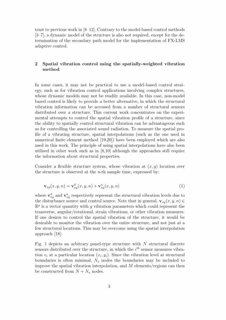
Fig. 1 depicts an arbitrary panel-type structure with N structural discretesensors distributed over the structure, in which the ith sensor measures vibra-tion vi at a particular location (xi, yi). Since the vibration level at structuralboundaries is often minimal, No nodes the boundaries may be included toimprove the spatial vibration interpolation, and M elements/regions can thenbe constructed from N + No nodes.
3
Fig. 1. A panel structure with N structural sensors and No nodes at structuralboundaries. The vibration level measured by the ith sensor at location (xi, yi) isvi. The mth element has local coordinates of (x(m), y(m)) and is constructed from 4nodes in this example.
For the mth element/region with local coordinates of (x(m), y(m)), the vibrationlevel v(m)
xy at any location (x(m), y(m)) within the element can be estimated fromsensor measurements. If l sensors are used to construct nodes for mth element,v(m)
xy ∈ Rg will be the estimated elemental vibration profile which are based
from vibration measurements obtained from the sensors, v(m):
v(m)xy (x(m), y(m), n) = H(x(m), y(m))v(m)(n) (2)
where v(m) consists of a group of l vibration measurements associated withthe mth element, and H(x(m), y(m)) is a g × l interpolation function matrix.
Transforming the local coordinates into the global coordinates using a lineartransformation matrix, the vibration profile can be shown to be in the formof [18]:
vxy(x, y, n)=M(x, y)v(n) (3)
where v ∈ R(N+No) consists of vibration measurements vi and vibrations ob-
served at the nodes.
The vibration at each (x, y) location can now be estimated from:
vxy(x, y, n) = M(x, y)vd(x, y, n) + M(x, y)vu(x, y, n) (4)
where vd and vu are the vibration signals measured at sensors and at the re-dundant structural boundary nodes, due to the disturbance source and control
4

source respectively.
2.1 Vibration control at certain spatial regions using spatial weighting
Having obtained the estimated vibration across the structure, structural re-gions that needs to be controlled can be emphasised using a continuous spatialweighting function, whose values can continuously vary across the structuredepending on the control requirement. For instance, transverse vibration atone region may need to be suppressed to reduced sound/noise radiation, whileat other region, strain vibration may be suppressed for improvement of struc-tural fatigue performance. A different spatial weighting function can then beemployed for each vibration parameter (e.g. transverse or strain vibration)whose high weighting values are given to regions with high control impor-tance.
In this case, a spatial weighting matrix can be introduced to reflect the spatialregions of interest for vibration control. A real-symmetric spatial weightingmatrix Q(x, y) continuous in (x, y) can be introduced where Q(x, y) > 0 forall locations (x, y) ∈ R, where R is the structural region of interest. Thisweighting function can be constructed using polynomial functions in (x, y).The simplest structure for matrix Q(x, y) is a diagonal weighting matrix whosediagonal elements represent the spatial weighting functions for the associatedvibration parameters to be controlled.
Thus, one can construct an objective function representing the spatially-weighted vibration energy, which can be minimised using active control strate-gies [18]. In this case, the instantaneous spatially-weighted vibration energyat the n-th sample time can be constructed as follows:
∫
RvT
xy(x, y, n)Q(x, y)vxy(x, y, n)dR =
(vd(n) + vu(n))T(
∫
RMT (x, y)Q(x, y)M(x, y)dR
)
(vd(n) + vu(n)) . (5)
The above integral term can be approximated by:
Θ=∫
RMT (x, y)Q(x, y)M(x, y)dR + α I
=UVUT (6)
where V and U are the eigenvalue and eigenvector matrices obtained fromthe eigenvalue decomposition of matrix Θ respectively. Here, α > 0 is a smallpositive scalar and I is an identity matrix with appropriate dimensions. Note
5
that since the first term in Eq. (6) is integrated over the entire surface of thestructure, the integral term is generally a positive definite matrix. However,due to rounding errors that might occur during the numerical integration, theterm might consist of a number of small negative eigenvalues which is whyα is used to shift the eigenvalues of
∫
R MT (x, y)Q(x, y)M(x, y)dR to ensurethe positive definiteness of matrix Θ. Since only few dominant eigenvalueswill be used for control, the use of α would not impact the spatial controlperformance, as will be seen in the experimental results presented later.
Note that having computed the integral term in Eq. (6), the dimensions of theterm can be condensed by removing the appropriate rows and columns thatcorrespond to the associated No nodes, which are redundant since vibrations atthe nodes (structural boundaries) are minimal [18]. The condensation reducesthe dimensions of the term from N + No to N . Now, v ∈ R
N , which consistsof vibration measurements at sensors vi, can be used for the rest of discussionin this work.
To simplify the control implementation, only a limited number of the largesteigenvalues of Θ are actually needed for control. Suppose that V and U arereduced in size using the eigenvalue-discarding process such that they now con-tain only a reduced number of eigenvalues and eigenvectors [18]. The trans-formed signal q(n) can now be obtained from the reduced eigenvector andeigenvalue matrices, V and U:
q(n) = Ωv(n) = V1/2UT v(n). (7)
It can be observed that this signal represents the spatially-weighted vibrationof the entire structure. Thus, an active control strategy that minimises theenergy of this signal would lead to the reduction of the spatially-weightedstructural vibration, i.e. reduction of vibration particularly at certain spa-tial regions with high weighting values. This instantaneous spatially-weightedvibration energy can now be approximated as follows:
∫
RvT
xy(n)Q(x, y)vxy(n)dR≈qT (n)q(n)
= (Ω (vd(n) + vu(n)))T (Ω (vd(n) + vu(n)))(8)
where vd and vu are the vibration signals measured at sensors due to thedisturbance source and control source respectively.
6
2.2 Adaptive spatial control using the FX-LMS adaptive control method
Next, the adaptive spatial control implementation using the spatial signalq(n) can be developed. Let P(n) and S(n) respectively represent the impulseresponses at the sensor locations associated with the disturbance d(n) andcontrol input u(n). The spatial signal q(n) can be obtained from:
q(n) = ΩP(n) ∗ d(n) + ΩS(n) ∗ u(n) (9)
where ∗ signifies the linear convolution.
Consider the case, where the dimension of the spatial signal q(n) is reducedfrom potentially N (since N sensors are used) to Nm after the eigenvalue-discarding approach mentioned in Eq. (7). That is, the first Nm dominanteigenvalues are used for the determination of V and U. Suppose there are S
disturbance signals, J reference signals and K control input signals, with theFinite Impulse Response (FIR) adaptive filters using L taps are utilised foradaptive spatial control.
Let the relevant signals be:
d(n) = [d1(n) . . . dS(n)]T
q(n) = [q1(n) . . . qNm(n)]T
x(n) =[
xT1 (n) . . .xT
J (n)]T
xj(n) = [xj(n) . . . xj(n − L + 1)]T , j = 1, . . . , J
u(n) = [u1(n) . . . uK(n)]T
w(n)=[
wT1 (n) . . .wT
K(n)]T
wk(n) = [wk1(n) . . .wkJ(n)]T , k = 1, . . . , K
wkj(n) = [wkj,0(n) . . .wkj,L−1(n)]T , k = 1, . . . , K; j = 1, . . . , J (10)
where d(n) ∈ RS,q(n) ∈ R
Nm ,x(n) ∈ RJL,u(n) ∈ R
K and w(n) ∈ RJLK
are respectively the disturbance signal, spatial signal, reference signal, controlinput signal and FIR control coefficients.
The control input can be calculated from filtering the reference signals withthe adaptive FIR filter [21]:
u(n) = XT (n)w(n) (11)
where X ∈ RJKL×K:
7

X=
x(n) · · · 0...
. . . 0
0 0 x(n)
. (12)
After the substitution of Eq. (11) into Eq. (9), the spatial signal is derivedfrom:
q(n) =ΩP(n) ∗ d(n) − ΩS(n) ∗ u(n)
=ΩP(n) ∗ d(n) − ΩS(n) ∗(
XT (n)w(n))
(13)
where P(n) contains the N × S impulse response functions for the primarypath; S(n) contains the N × K impulse response functions for the secondarypath; and Ω is the Nm × N spatial filter matrix.
The FIR filter coefficients in w(n) are now adapted using the gradient-basedoptimisation. Since the minimisation of the spatially-weighted vibration is ofinterest, it can be shown that the optimisation gradient has the form of:
5
(∫
RvT
xy(x, y, n)Q(x, y)vxy(x, y, n)dR
)
≈5(
qT (n)q(n))
=−2(
ΩST (n) ~ x(n))
q(n)(14)
where ~ denotes the Kronecker product convolution and Eq. (8) has beenutilised in the derivations.
The adaptation process for the spatial control can now be obtained from:
w(n + 1)=w(n) −µ
25
(
qT (n)q(n))
=w(n) + µXr(n)q(n) (15)
where µ is the convergence coefficient and Xr(n) is:
Xr(n)=ΩST (n) ~ x(n) (16)
and S(n) is the model/estimate of the secondary path’s impulse responses.
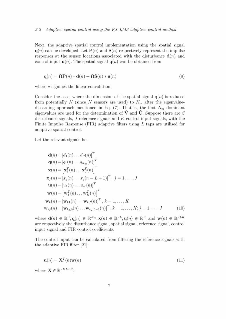
The implementation of the FX-LMS algorithm is illustrated in Fig. 2, wherethe spatial signal can be obtained from the filtering process of the sensors sig-nals by the spatial filter Ω. An LMS algorithm using the adaptive algorithm inEq. (15) is utilised to optimise the control coefficients w(n) that minimises the
8
instantaneous spatially-weighted vibration energy. The following section willdescribe the implementation of the spatial control strategy to a rectangularpanel which is the main part of the work.
Fig. 2. FX-LMS adaptive spatial control diagram.
3 Experimental implementation of spatial control on a panel struc-ture
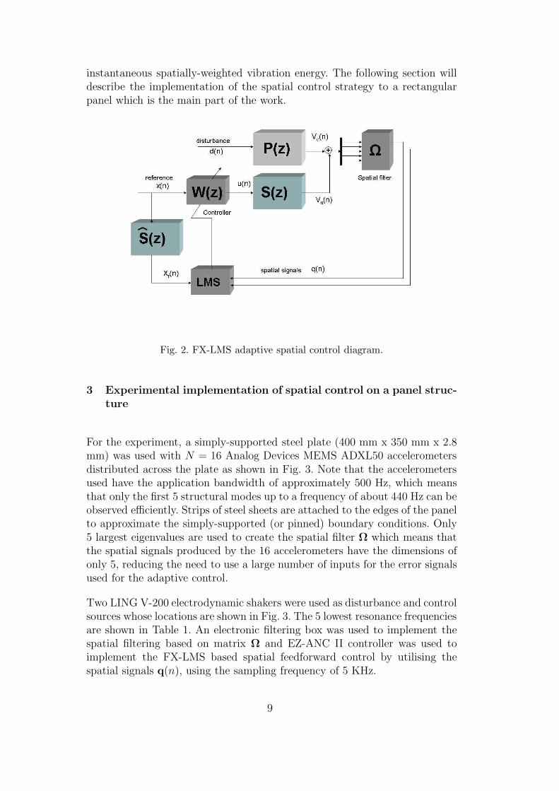
For the experiment, a simply-supported steel plate (400 mm x 350 mm x 2.8mm) was used with N = 16 Analog Devices MEMS ADXL50 accelerometersdistributed across the plate as shown in Fig. 3. Note that the accelerometersused have the application bandwidth of approximately 500 Hz, which meansthat only the first 5 structural modes up to a frequency of about 440 Hz can beobserved efficiently. Strips of steel sheets are attached to the edges of the panelto approximate the simply-supported (or pinned) boundary conditions. Only5 largest eigenvalues are used to create the spatial filter Ω which means thatthe spatial signals produced by the 16 accelerometers have the dimensions ofonly 5, reducing the need to use a large number of inputs for the error signalsused for the adaptive control.
Two LING V-200 electrodynamic shakers were used as disturbance and controlsources whose locations are shown in Fig. 3. The 5 lowest resonance frequenciesare shown in Table 1. An electronic filtering box was used to implement thespatial filtering based on matrix Ω and EZ-ANC II controller was used toimplement the FX-LMS based spatial feedforward control by utilising thespatial signals q(n), using the sampling frequency of 5 KHz.
9
0 0.05 0.1 0.15 0.2 0.25 0.3 0.35 0.40
0.05
0.1
0.15
0.2
0.25
0.3
0.35
x−axis [m]
y−ax
is [m
]
disturbance
control actuator
accelerometers
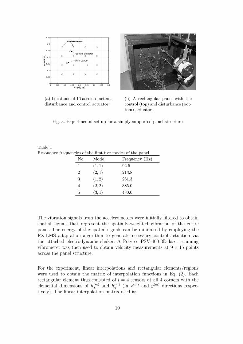
(a) Locations of 16 accelerometers,disturbance and control actuator.
(b) A rectangular panel with thecontrol (top) and disturbance (bot-tom) actuators.
Fig. 3. Experimental set-up for a simply-supported panel structure.
Table 1Resonance frequencies of the first five modes of the panel
No. Mode Frequency (Hz)
1 (1, 1) 92.5
2 (2, 1) 213.8
3 (1, 2) 261.3
4 (2, 2) 385.0
5 (3, 1) 430.0
The vibration signals from the accelerometers were initially filtered to obtainspatial signals that represent the spatially-weighted vibration of the entirepanel. The energy of the spatial signals can be minimised by employing theFX-LMS adaptation algorithm to generate necessary control actuation viathe attached electrodynamic shaker. A Polytec PSV-400-3D laser scanningvibrometer was then used to obtain velocity measurements at 9 × 15 pointsacross the panel structure.
For the experiment, linear interpolations and rectangular elements/regionswere used to obtain the matrix of interpolation functions in Eq. (2). Eachrectangular element thus consisted of l = 4 sensors at all 4 corners with theelemental dimensions of h(m)
x and h(m)y (in x(m) and y(m) directions respec-
tively). The linear interpolation matrix used is:
10

H(x(m), y(m))=
1 −
(
x(m)
h(m)x
)
1 −
(
y(m)
h(m)y
)
(
x(m)
h(m)x
)
1 −(
y(m)
h(m)y
)
1 −
(
x(m)
h(m)x
) (
y(m)
h(m)y
)
(
x(m)
h(m)x
) (
y(m)
h(m)y
)
T
. (17)
Two normalised scalar spatial weightings Q1(x, y) > 0 and Q2(x, y) > 0 werechosen for the experiment as shown in Fig. 4 and spatial filter matrix Ω canbe obtained from Eq. (7). Note that the two weighting functions have differentstructural regions of interest as reflected by the high weighting values. In thiscase, spatial weightings 1 and 2 have maximum weightings at (0.133m,0.110m)and (0.265m,0.100m) respectively. Note that the centre of the panel is locatedat (0.200m,0.175m) so the peak of spatial weighting 1 occurs closer to the cen-tre of the panel compared to that of spatial weighting 2. The purpose of thesespatial weightings is to target regions where vibration control is desirable.
00.1
0.20.3
0.4
00.1
0.2
0.3
0
0.2
0.4
0.6
0.8
1
x [m]y [m]
(a) spatial weighting 1, Q1(x, y)
00.1
0.20.3
0.4
00.1
0.2
0.3
0
0.2
0.4
0.6
0.8
1
x [m]y [m]
(b) spatial weighting 2, Q2(x, y)
Fig. 4. Two spatial weighting functions used in the experiment.
3.1 Spatial tonal control of a panel structure
In this section, vibration control experiments at a single excitation frequencyhas been performed to observe the effectiveness of spatial tonal control. Sincesignificant vibration occurs at or near the structural resonance frequencies,the experiments target a number of resonance frequencies.
11

Spatial control on mode (1,1) at 92.5 Hz.
(a) no control - spatial vibration pro-file of mode (1,1)
(b) with control - experiment
x−axis [m]
y−ax
is [m
]
0 0.05 0.1 0.15 0.2 0.25 0.3 0.35 0.40
0.05
0.1
0.15
0.2
0.25
0.3
0.35
0.05
0.1
0.15
0.2
0.25
0.3
0.35
0.4
0.45
0.5
(c) with control - simulation
Fig. 5. Experiment using the spatial weighting 1, Q1(x, y), for mode (1,1) at 92.5Hz. The gray-scale bar represents the percentage of vibration level with respect tothe maximum un-controlled vibration.
The first experiment considers the first structural mode (1,1) at 92.5 Hz. TheRMS (root mean squared) vibration profile of the panel with and withoutcontrol are shown in Fig. 5 for the control case using the spatial weighting 1.It can be seen that the vibration at the structural region of interest (at thelower left-hand-side (LHS) corner of the panel) has been reduced more than theupper region as expected. The vibration nodal line exists closer to the region
12
of interest, which implies that the upper and lower regions vibrate in oppositedirections (i.e. with 180o phase difference). The simulation result based onan idealised simply-supported panel using an optimal spatial tonal controlapproach is also shown in Fig. 5(c). It is interesting to note that the spatialvibration profiles obtained from the experiment and the idealised model aresimilar. At higher frequencies, however, more pronounced differences betweenthe experiment and simulation can be expected.
(a) with control - experiment
x−axis [m]
y−ax
is [m
]
0 0.05 0.1 0.15 0.2 0.25 0.3 0.35 0.40
0.05
0.1
0.15
0.2
0.25
0.3
0.35
0.05
0.1
0.15
0.2
0.25
0.3
0.35
0.4
(b) with control - simulation
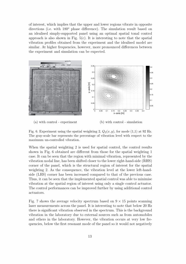
Fig. 6. Experiment using the spatial weighting 2, Q2(x, y), for mode (1,1) at 92 Hz.The gray-scale bar represents the percentage of vibration level with respect to themaximum un-controlled vibration.
When the spatial weighting 2 is used for spatial control, the control resultsshown in Fig. 6 obtained are different from those for the spatial weighting 1case. It can be seen that the region with minimal vibration, represented by thevibration nodal line, has been shifted closer to the lower right-hand-side (RHS)corner of the panel, which is the structural region of interest for the spatialweighting 2. As the consequence, the vibration level at the lower left-hand-side (LHS) corner has been increased compared to that of the previous case.Thus, it can be seen that the implemented spatial control was able to minimisevibration at the spatial region of interest using only a single control actuator.The control performances can be improved further by using additional controlactuators.
Fig. 7 shows the average velocity spectrum based on 9 × 15 points scanninglaser measurements across the panel. It is interesting to note that below 20 Hzthere is significant vibration observed in the spectrum. This is the backgroundvibration in the laboratory due to external sources such as from automobilesand others in the laboratory. However, the vibration occurs at very low fre-quencies, below the first resonant mode of the panel so it would not negatively
13

affect the control experiments. For both control cases using different spatialweightings, the averaged vibration reductions of the panel are approximately35 and 36 dB at 92.5 Hz respectively for spatial weightings 1 and 2. The re-sults can be expected since the overall panel vibration has also been reduced,however the region of interest has received more vibration reduction as shownin Figs. 5 and 6.
Spatial control on mode (2,1) at 213.8 Hz.
Experimental results for mode (2,1) at 213.8 Hz are shown in Figs. 8 and 9for spatial control using spatial weightings 1 and 2 respectively. After control,it can be observed that the regions of low vibration actually occured arounda diagonal nodal line over the panel. The results can be expected since for thespatial weighting 1 case, the diagonal nodal line cuts across the lower LHSregion, which is the region of interest for vibration minimisation. Similarly,the spatial weighting 2 case results in Fig. 9 reflect the vibration minimisationthat targets the lower RHS region. Simulation results also describe similarpatterns of results for both control cases. Fig. 10 shows the average velocityspectrum across the panel, where for both control cases, the average vibrationreductions of the panel are similar at approximately 22.5 dB at the resonancefrequency of mode (2,1) of 213.8 Hz.
Spatial control on mode (1,2) at 261.3 Hz.
Control results for mode (1,2) at 261.3 Hz are shown in Figs. 11 and 12 forspatial control using spatial weightings 1 and 2 respectively. Again a diagonalnodal line indicates the location where the vibration level is lower than that atother regions. The implemented controller has modified the vibration profileof the panel at that particular frequency so that the structure has a minimalspatially-weighted vibration energy. Simulation results also indicate a similarcontrol behaviour, indicating the actual control results agree well with theidealised optimal spatial control results. The average velocity spectrum acrossthe panel is shown in Fig. 13. The average panel vibration reduction levels forthe spatial weighting 1 and 2 cases are respectively 15.5 and 19.5 dB at theresonance frequency of mode (1,2) of 261.3 Hz.
Spatial control on mode (2,2) at 385.0 Hz.
The experimental results for spatial control on the mode (2,2) at 385.0 Hz areshown in Figs. 14 and 15 for spatial weightings 1 and 2 respectively. There arenow 2 main nodal lines occuring across the controlled panel. For the spatialweighting 1 case, a nodal line occured at lower LHS of the panel, cuttingacross the region with the maximum spatial weighting at (0.133m,0.110m).For spatial weighting 2 case, a nearly vertical nodal line (compared to Fig. 14)occured closer to the RHS of the panel so that the vibration at the lower RHScan be supressed further. The nodal line also cuts across the region around
14

(a) no control
(b) spatial control with spatial weighting 1
(c) spatial control with spatial weighting 2
Fig. 7. The average velocity spectrum of the panel for the un-controlled case, the spa-tially controlled case with Q1(x, y), and the spatially controlled case with Q2(x, y):for mode (1,1) at 92.5 Hz.
(0.265m,0.100m) which has the maximum weighting for the spatial weighting 2case.
15
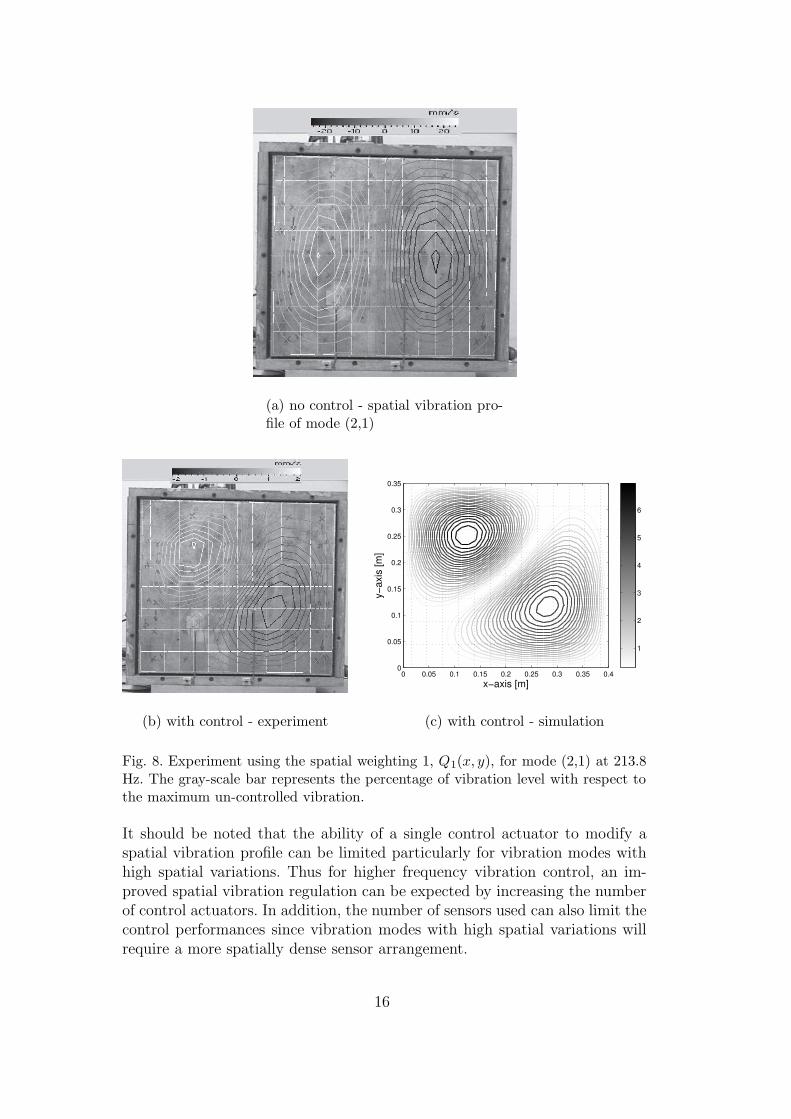
(a) no control - spatial vibration pro-file of mode (2,1)
(b) with control - experiment
x−axis [m]
y−ax
is [m
]
0 0.05 0.1 0.15 0.2 0.25 0.3 0.35 0.40
0.05
0.1
0.15
0.2
0.25
0.3
0.35
1
2
3
4
5
6
(c) with control - simulation
Fig. 8. Experiment using the spatial weighting 1, Q1(x, y), for mode (2,1) at 213.8Hz. The gray-scale bar represents the percentage of vibration level with respect tothe maximum un-controlled vibration.
It should be noted that the ability of a single control actuator to modify aspatial vibration profile can be limited particularly for vibration modes withhigh spatial variations. Thus for higher frequency vibration control, an im-proved spatial vibration regulation can be expected by increasing the numberof control actuators. In addition, the number of sensors used can also limit thecontrol performances since vibration modes with high spatial variations willrequire a more spatially dense sensor arrangement.
16
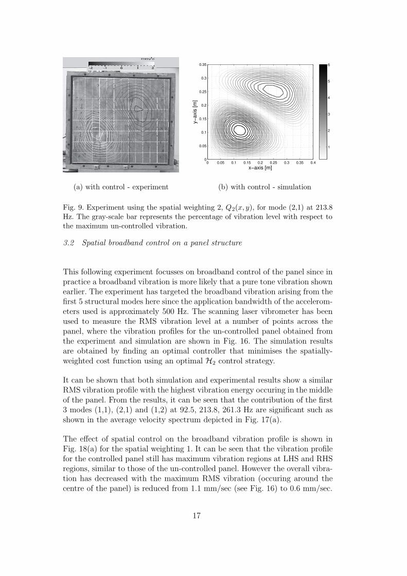
(a) with control - experiment
x−axis [m]
y−ax
is [m
]
0 0.05 0.1 0.15 0.2 0.25 0.3 0.35 0.40
0.05
0.1
0.15
0.2
0.25
0.3
0.35
1
2
3
4
5
6
(b) with control - simulation
Fig. 9. Experiment using the spatial weighting 2, Q2(x, y), for mode (2,1) at 213.8Hz. The gray-scale bar represents the percentage of vibration level with respect tothe maximum un-controlled vibration.
3.2 Spatial broadband control on a panel structure
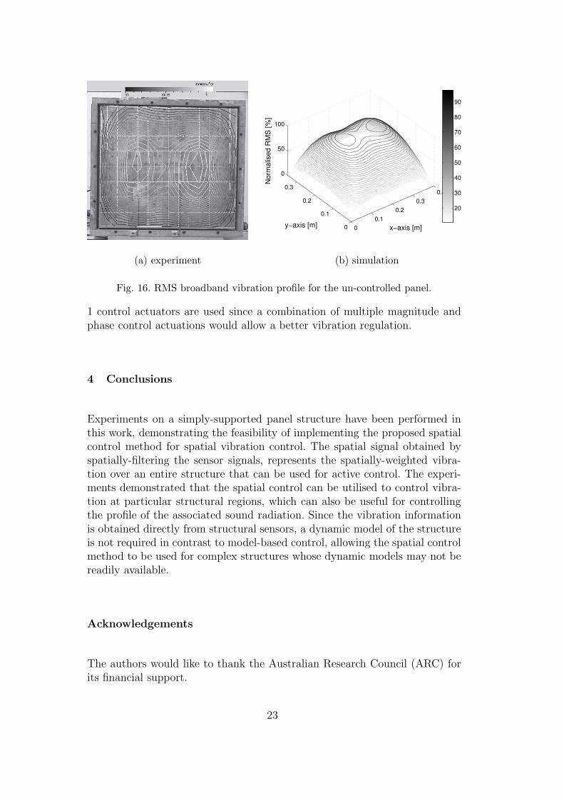
This following experiment focusses on broadband control of the panel since inpractice a broadband vibration is more likely that a pure tone vibration shownearlier. The experiment has targeted the broadband vibration arising from thefirst 5 structural modes here since the application bandwidth of the accelerom-eters used is approximately 500 Hz. The scanning laser vibrometer has beenused to measure the RMS vibration level at a number of points across thepanel, where the vibration profiles for the un-controlled panel obtained fromthe experiment and simulation are shown in Fig. 16. The simulation resultsare obtained by finding an optimal controller that minimises the spatially-weighted cost function using an optimal H2 control strategy.
It can be shown that both simulation and experimental results show a similarRMS vibration profile with the highest vibration energy occuring in the middleof the panel. From the results, it can be seen that the contribution of the first3 modes (1,1), (2,1) and (1,2) at 92.5, 213.8, 261.3 Hz are significant such asshown in the average velocity spectrum depicted in Fig. 17(a).
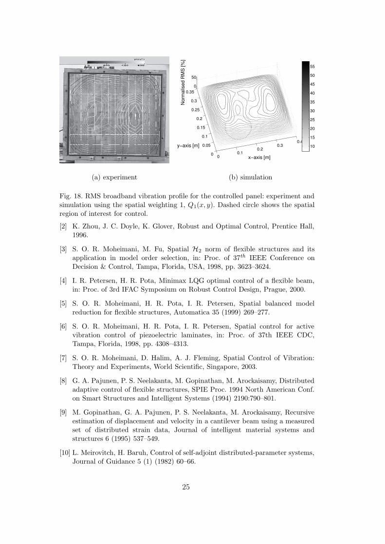
The effect of spatial control on the broadband vibration profile is shown inFig. 18(a) for the spatial weighting 1. It can be seen that the vibration profilefor the controlled panel still has maximum vibration regions at LHS and RHSregions, similar to those of the un-controlled panel. However the overall vibra-tion has decreased with the maximum RMS vibration (occuring around thecentre of the panel) is reduced from 1.1 mm/sec (see Fig. 16) to 0.6 mm/sec.
17
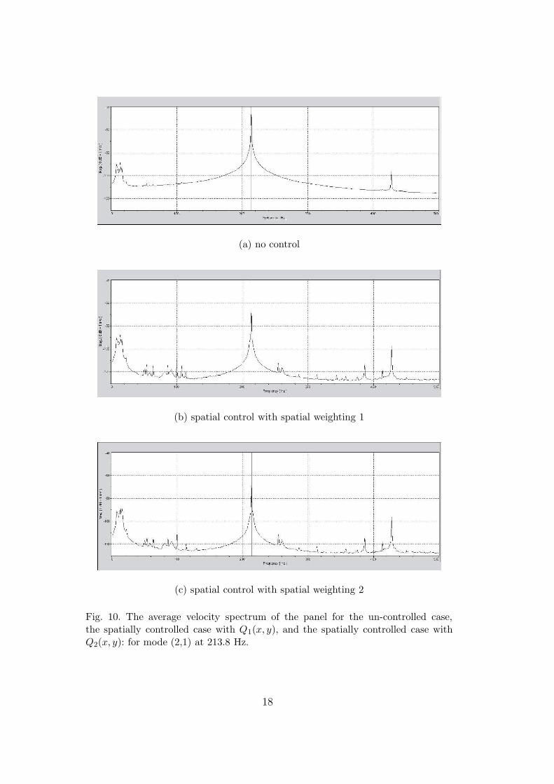
(a) no control
(b) spatial control with spatial weighting 1
(c) spatial control with spatial weighting 2
Fig. 10. The average velocity spectrum of the panel for the un-controlled case,the spatially controlled case with Q1(x, y), and the spatially controlled case withQ2(x, y): for mode (2,1) at 213.8 Hz.
18

(a) no control - spatial vibration pro-file of mode (1,2)
(b) with control - experiment
x−axis [m]
y−ax
is [m
]
0 0.05 0.1 0.15 0.2 0.25 0.3 0.35 0.40
0.05
0.1
0.15
0.2
0.25
0.3
0.35
5
10
15
20
25
(c) with control - simulation
Fig. 11. Experiment using the spatial weighting 1, Q1(x, y), for mode (1,2) at 261.3Hz. The gray-scale bar represents the percentage of vibration level with respect tothe maximum un-controlled vibration.
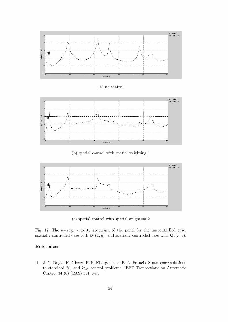
Furthermore, note that LHS vibration peak has been shifted up relative to theRHS vibration peak by the control action. The results can be expected sincethe lower LHS region has high weighting reflected by the spatial weighting 1.A similar vibration profile can be observed from the simulation as depicted inFig. 18(b) where the RHS vibration peak has been also shifted up by controlaction, where the region of interest is shown with a circle. From Fig. 17(b), theaverage vibration reduction achieved is 8, 7, 12 and 11 dB for the first 4 modes.
19

(a) with control - experiment
x−axis [m]
y−ax
is [m
]
0 0.05 0.1 0.15 0.2 0.25 0.3 0.35 0.40
0.05
0.1
0.15
0.2
0.25
0.3
0.35
2
4
6
8
10
12
14
16
18
(b) with control - simulation
Fig. 12. Experiment using the spatial weighting 2, Q2(x, y), for mode (1,2) at 261.3Hz. The gray-scale bar represents the percentage of vibration level with respect tothe maximum un-controlled vibration.
There is a slight 1 dB increase observed for the 5th mode (3,1) at 430 Hz. Notethat since the broadband case involve simultaneous excitations of a number ofstructural modes, the spatial vibration variation is less pronounced than thatfor tonal cases. In addition, increasing the number of control sources wouldalso improve the spatial control performance in targeting specific regions.
The broadband spatial control results for the spatial weighting 2 is shown inFig. 19. In this case, the vibration peak at the RHS region has been shiftedup since the spatial region of interest is located at the lower RHS regionof the panel. The overall vibration has also decreased with the maximumRMS vibration is reduced from 1.1 mm/sec to 0.6 mm/sec. Note that thesimulation results in Fig. 19(b) shows a similar vibration profile as observedfrom the experiments. When the control gain is increased, Fig. 19(c) showsthe broadband energy is further reduced in the lower RHS region of interest,so that the vibration in the region shown in a circle can be further reduced.From Fig. 17(c), the averaged vibration reduction achieved is 3, 9, 11 and 14dB for the first 4 modes, while a slight 1 dB increase is observed for the 5thmode (3,1) at 430 Hz.
It is interesting to compare the vibration reduction performance of both con-trol cases shown in Figs. 17(b) and (c). Note that the peak of spatial weight-ing 1 at (0.133m,0.11m) is closer to the centre of panel at (0.20m,0.175m),which is also the vibration peak for mode (1,1). In contrast, the peak of spa-tial weighting 2 is closer to the lower RHS corner of the panel. Consequently,the controller for the spatial weighting 1 concentrates more in reducing thestrength of mode (1,1) (by 8 dB) compared to that for the spatial weight-
20
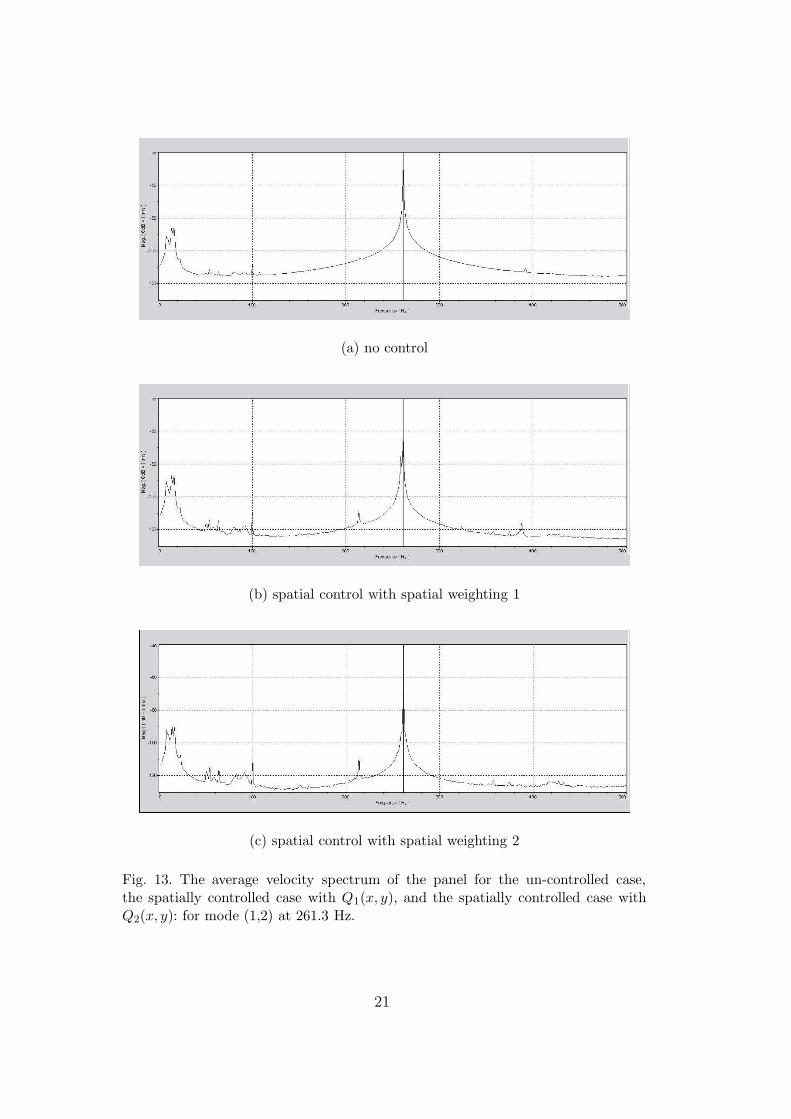
(a) no control
(b) spatial control with spatial weighting 1
(c) spatial control with spatial weighting 2
Fig. 13. The average velocity spectrum of the panel for the un-controlled case,the spatially controlled case with Q1(x, y), and the spatially controlled case withQ2(x, y): for mode (1,2) at 261.3 Hz.
21

(a) with control - experiment
x−axis [m]
y−ax
is [m
]
0 0.05 0.1 0.15 0.2 0.25 0.3 0.35 0.40
0.05
0.1
0.15
0.2
0.25
0.3
0.35
2
4
6
8
10
12
(b) with control - simulation
Fig. 14. Experiment using the spatial weighting 1, Q1(x, y), for mode (2,2) at 385.0Hz. The gray-scale bar represents the percentage of vibration level with respect tothe maximum un-controlled vibration.
(a) with control - experiment
x−axis [m]
y−ax
is [m
]
0 0.05 0.1 0.15 0.2 0.25 0.3 0.35 0.40
0.05
0.1
0.15
0.2
0.25
0.3
0.35
1
2
3
4
5
6
7
8
9
(b) with control - simulation
Fig. 15. Experiment using the spatial weighting 2, Q2(x, y), for mode (2,2) at 385.0Hz. The gray-scale bar represents the percentage of vibration level with respect tothe maximum un-controlled vibration.
ing 2 (by only 3 dB). In contrast, the controller for the spatial weighting 2attempts to reduce the strength of mode (2,2) (by 14 dB) more than that forthe spatial weighting 1 (by only 11 dB) since vibration mode(2,2) also has themaximum transverse vibration very close to the region of interest (at the lowerRHS corner of the panel). In general, therefore, the spatial control attemptsto control vibration modes that have dominant contributions to vibration atthe region of interest. Improved results can also be expected when more than
22
(a) experiment
00.1
0.20.3
0.4
0
0.1
0.2
0.3
0
50
100
Nor
mal
ised
RM
S [%
]
x−axis [m]y−axis [m]
20
30
40
50
60
70
80
90
(b) simulation
Fig. 16. RMS broadband vibration profile for the un-controlled panel.
1 control actuators are used since a combination of multiple magnitude andphase control actuations would allow a better vibration regulation.
4 Conclusions
Experiments on a simply-supported panel structure have been performed inthis work, demonstrating the feasibility of implementing the proposed spatialcontrol method for spatial vibration control. The spatial signal obtained byspatially-filtering the sensor signals, represents the spatially-weighted vibra-tion over an entire structure that can be used for active control. The experi-ments demonstrated that the spatial control can be utilised to control vibra-tion at particular structural regions, which can also be useful for controllingthe profile of the associated sound radiation. Since the vibration informationis obtained directly from structural sensors, a dynamic model of the structureis not required in contrast to model-based control, allowing the spatial controlmethod to be used for complex structures whose dynamic models may not bereadily available.
Acknowledgements
The authors would like to thank the Australian Research Council (ARC) forits financial support.
23
(a) no control
(b) spatial control with spatial weighting 1
(c) spatial control with spatial weighting 2
Fig. 17. The average velocity spectrum of the panel for the un-controlled case,spatially controlled case with Q1(x, y), and spatially controlled case with Q2(x, y).
References
[1] J. C. Doyle, K. Glover, P. P. Khargonekar, B. A. Francis, State-space solutionsto standard H2 and H∞ control problems, IEEE Transactions on AutomaticControl 34 (8) (1989) 831–847.
24
(a) experiment
00.1
0.20.3
0.4
0
0.05
0.1
0.15
0.2
0.25
0.3
0.350
50
x−axis [m]
y−axis [m]
Nor
mal
ised
RM
S [%
]
10
15
20
25
30
35
40
45
50
55
(b) simulation
Fig. 18. RMS broadband vibration profile for the controlled panel: experiment andsimulation using the spatial weighting 1, Q1(x, y). Dashed circle shows the spatialregion of interest for control.
[2] K. Zhou, J. C. Doyle, K. Glover, Robust and Optimal Control, Prentice Hall,1996.
[3] S. O. R. Moheimani, M. Fu, Spatial H2 norm of flexible structures and itsapplication in model order selection, in: Proc. of 37th IEEE Conference onDecision & Control, Tampa, Florida, USA, 1998, pp. 3623–3624.
[4] I. R. Petersen, H. R. Pota, Minimax LQG optimal control of a flexible beam,in: Proc. of 3rd IFAC Symposium on Robust Control Design, Prague, 2000.
[5] S. O. R. Moheimani, H. R. Pota, I. R. Petersen, Spatial balanced modelreduction for flexible structures, Automatica 35 (1999) 269–277.
[6] S. O. R. Moheimani, H. R. Pota, I. R. Petersen, Spatial control for activevibration control of piezoelectric laminates, in: Proc. of 37th IEEE CDC,Tampa, Florida, 1998, pp. 4308–4313.
[7] S. O. R. Moheimani, D. Halim, A. J. Fleming, Spatial Control of Vibration:Theory and Experiments, World Scientific, Singapore, 2003.
[8] G. A. Pajunen, P. S. Neelakanta, M. Gopinathan, M. Arockaisamy, Distributedadaptive control of flexible structures, SPIE Proc. 1994 North American Conf.on Smart Structures and Intelligent Systems (1994) 2190:790–801.
[9] M. Gopinathan, G. A. Pajunen, P. S. Neelakanta, M. Arockaisamy, Recursiveestimation of displacement and velocity in a cantilever beam using a measuredset of distributed strain data, Journal of intelligent material systems andstructures 6 (1995) 537–549.
[10] L. Meirovitch, H. Baruh, Control of self-adjoint distributed-parameter systems,Journal of Guidance 5 (1) (1982) 60–66.
25

(a) experiment
00.1
0.20.3
0.4
0
0.05
0.1
0.15
0.2
0.25
0.3
0.350
50
x−axis [m]
y−axis [m]
Nor
mal
ised
RM
S [%
]
10
15
20
25
30
35
40
45
50
55
60
(b) simulation - control gain 1
00.1
0.20.3
0.4
0
0.05
0.1
0.15
0.2
0.25
0.3
0.350
50
x−axis [m]
y−axis [m]
Nor
mal
ised
RM
S [%
]
10
15
20
25
30
35
40
45
50
55
60
(c) simulation - control gain 2
Fig. 19. RMS broadband vibration profile for the controlled panel: experiment andsimulation using the spatial weighting 2, Q2(x, y). Dashed circles show the spatialregions of interest for control
[11] L. Meirovitch, H. Baruh, The implementation of modal filters for control ofstructures, Journal of Guidance 8 (6) (1985) 707–716.
[12] L. Meirovitch, Some problems associated with the control of distributedstructures, Journal of Optimization Theory and Applications 54 (1) (1987) 1–21.
[13] S. Collins, D. W. Miller, A. Von Flotow, Distributed sensors as spatial filtersin active structural control, Journal of Sound and Vibration 173 (4) (1994)471–501.
[14] R. L. Clark, C. R. Fuller, Modal sensing of efficient acoustic radiators withpolyvinylidene fluoride distributed sensors in active structural acoustic controlapproaches, Journal of Acoustical Society of America 91 (6) (1992) 3321–3329.
26

[15] S. D. Snyder, N. Tanaka, On feedforward active control of sound and vibrationusing vibration error signals, Journal of the Acoustical Society of America 94 (4)(1993) 2181–2192.
[16] F. Charette, A. Berry, C. Guigou, Active control of sound radiation from aplate using a polyvinylidene fluoride volume displacement sensor, Journal ofthe Acoustical Society of America 103 (3) (1998) 1493–1503.
[17] A. Preumont, A. Francois, P. De Man, N. Loix, K. Henrioulle, Distributedsensors with piezoelectric films in design of spatial filters for structural control,Journal of Sound and Vibration 282 (2005) 701–712.
[18] D. Halim, B. S. Cazzolato, A multiple-sensor method for control of structuralvibration with spatial objectives, Journal of Sound and Vibration 296 (2006)226–242.
[19] K. J. Bathe, E. L. Wilson, Numerical Methods in Finite Element Analysis,Prentice Hall, Englewood Cliffs, New Jersey, 1976.
[20] Y. K. Cheung, A. Y. T. Leung, Finite Element Methods in Dynamics, SciencePress; Kluwer Academic Publishers, Beijing, New York; Dordrecht, Boston,1991.
[21] S. M. Kuo, D. R. Morgan, Active Noise Control Systems: Algorithms and DSPImplementations, John Wiley & Sons, 1996.
27