Embed Size (px)
Citation preview

Acoustic Emission for Diagnosis of Train Rotating Systems
Professor Dr Andy TanChairman – Centre for Railway Infrastructure and Engineering
LKC Faculty of Engineering and ScienceUniversiti Tunku Abdul Rahman
Sungai Long, Cheras, 43000 KajangSelangor, Malaysia

• Part 1- Introduction to Railway in Malaysia
• Part 2- Acoustic Emission for diagnosis of train rotating system
Headquarters of the F.M.S. Railways at Kuala Lumpur - circa 1910.

The History of KTM Railway

Diesel trainsBased on 1m guage with total distance of the network at 1,699 km.
Launch its first diesel engine, a Class 15 Shutter, in 1948 and fully convert to diesel power between the 1950s and 1970s, and till recently.
Class 29 diesel locomotive at Gemas Railway Station (Sept. 2009), Dalian Locomotive

Electric TrainsElectric trains were only introduced in 1995
Electric locomotive ŠkodaChS4-109

Recent KTM Inter-city TrainsThe KTM West Coast Line between Singapore and Padang Besar, on to the Malaysian-Thai border.
The KTM East Coast Line between Gemas in Negri Sembilan and Tumpatin Kelantan and branches between Kuala Lumpur, Port Klang, and other cities in peninsular Malaysia.

Express Rail Link (ERL)Operate between Kuala Lumpur and International Airport KLIA and KLIA2. Maximum speed is about 160 km/h (99 mph) and distance of 57 km.
Operate in 14 April 2002 with a ridership of 6.6 M passenger in 2017
Rolling – 4x4 CRRC Changchun Articulated EMU and 4x4 Desiro ET 425 M Articulated EMU

Light Rapid Transit (LRT)The three light rapid transit lines in Kuala Lumpur are the Kelana Jaya Line, the Ampang Line and Sri Petaling Line.
The line was completely opened in 1998.

Kelana Jaya lineThe Kelana Jaya Line is a driver-less automatic system and is 46.4 km (29 mi) long, running between the northeastern suburbs of Kuala Lumpur and PetalingJaya to the west of Kuala Lumpur. Started operation 1999.
Bombadier Innovia Metro 300 trainServicing 37 stations, running
mostly on underground and elevated guideways. Fully automated Driverless

Ampang and Sri PetalinglinesThe third and fourth rapid transit lines in Klang Valley. The combined network comprises 45.1 kilometres of track (28 miles) with 36 stations, and is the first to use the standard gauge track and semi-automated trains in Klang Valley.
6-car CSR Zhuzhou Amy Articulated LRV

Mass Rapid Transit (MRT)Phase 1 (Sungai Buloh -Kajang started its operation in 15 December 2016. 47 km in distance serving a population of 1.2M people in the region.Ridership in 2017 – 2.25MConstruction cost estimated MYR36 billion
A Siemens Inspiro EMU stock

KL – Singapore HSR• Feasibility studies in 2006 and as of June 2007, the project cost
RM8 billion project would slash travel time from more than 6 hours to about 90 minutes.
• The main stumbling blocks, apart from costs, appears to be the JB-Woodlands Causeway.
• On January 2008, the government is still looking in the proposal and had yet to make a final decision.
• On 22 April 2008, the government announce that the project was put on hold indefinitely due to high cost.
• On March 2009, to revive the project again, it will seek to build the rail line on the coastline on the existing track.
• In September 2010, Malaysia and Singapore formalized the construction of HSR, officially agreed in February 2013 to go ahead and set a completion date of 2026.
• In May 2018, the newly-minted Prime Minister announced the cancellation of the project and will resume in Jan 2031.

Original time-lineThis was the planned timeline. However, the project was postponed by the Malaysian Government.•19 July 2016: Signing of MOU for KL–Singapore HSR project•August 2016: Singapore to call tender for advance engineering studies. Singapore–Malaysia joint tender for Joint Development Partner•13 December 2016: Bilateral agreement signed•Late 2017: Civil works and tender for private entity overseeing train and rail assets•2018–2025: Construction•Late 2023: International and domestic operators tender•2024–2026: Testing and commissioning•By December 31, 2026: Operations to begin
Chinese designedCRH380AL train
Japan’s high speed bullet trains, Shinkansen trains, has a top speed reaching up to 320 km/hr

Motivation• The benefits and challenges of AE for fault
detection• Peak Hold Down Sampling to resolve massive data
storage due to high sampling frequency• Normalization of signal response of different AE
sensors in multi-sensor application• Case study on diesel engine• Case study on mixer gearbox


Vibration vs. AE
massPZT
Vibration(1-20kHz)
PZT
Stress wave or AE(100kHz-1Mhz)
Accelerometer AE sensor

• Acoustic emissions are transient elastic waves generated by the rapid release of energy from localized sources within and on the surface of a material (up to 1MHz)
• Sources : crack initiation/propagation, friction, rubbing, impacting, turbulent flow
• Main benefits : high S/N ratio, crack detection, early detection of mechanical integrity
• Challenges : where multiple AE sources exist, global monitoring, hardware implementation
• Applications : cracks in structure(bridge, vessel, tank, pipeline etc.), bearings, seals, gearbox, diesel engines, leak detection, low speed machine
Acoustic Emissions

Piezoceramic Sensor and Actuator 1. Actuator – Induced Moment
+
+−=
ppbb
ppbbpb
tTEtTEWTEtTEtt
TdtxVTM)()(
)()(2
)(),()( 31
2. Sensor – Voltage Generated
)],(),([)( 12 xtyxtyktv ss ′−′=
Sensing Constantp
ppcps t
LWzEgk
231=

Peak Hold Down Sampling

Peak Hold Down Sampling• Due to low rotating speed and to capture sufficient data
for a few complete shaft rotations will end up with massive data storage at high sampling rate.
• Transmission of large amount of data for storage and analysis from remote sites will require massive data transfer and limitation of current technology.
• Traditional down sampling selects every ith sample at equal intervals and discard the rest of the data from the original data to reduce the data size and result in loss of vital information.
• Peak-Hold-Down-Sampling (PHDS) retains critical impulses due to bearing and gearbox defects in the time waveform.

PHDS Algorithm

Mathematical Description

• Main challenges in AE application to low speed machinery huge amount of data missing frequency information
• Peak Hold Down Sampling :o Detects high frequency impact information with very slow speed sampling
Peak Hold Down Sampling
0 0.1 0.2 0.3 0.4 0.5 0.6 0.7 0.8 0.9 1-2
0
2
0 0.1 0.2 0.3 0.4 0.5 0.6 0.7 0.8 0.9 1-2
0
2
0 0.1 0.2 0.3 0.4 0.5 0.6 0.7 0.8 0.9 1-2
0
2
0 0.1 0.2 0.3 0.4 0.5 0.6 0.7 0.8 0.9 1-2
0
2
0 0.1 0.2 0.3 0.4 0.5 0.6 0.7 0.8 0.9 1-2
0
2
0 0.1 0.2 0.3 0.4 0.5 0.6 0.7 0.8 0.9 1-2
0
2
0 0.1 0.2 0.3 0.4 0.5 0.6 0.7 0.8 0.9 1-2
0
2
0 0.1 0.2 0.3 0.4 0.5 0.6 0.7 0.8 0.9 1-2
0
2
Peak Hold Down Sampling Normal Down Sampling
Original
1/5
1/10
1/20

0 0.1 0.2 0.3 0.4 0.5 0.6 0.7 0.8 0.9 1-0.02
0
0.02
0 0.1 0.2 0.3 0.4 0.5 0.6 0.7 0.8 0.9 1-0.02
0
0.02
Measure
d A
E a
nd P
HD
S S
ignals
0 0.1 0.2 0.3 0.4 0.5 0.6 0.7 0.8 0.9 1-0.02
0
0.02
0 0.1 0.2 0.3 0.4 0.5 0.6 0.7 0.8 0.9 1-0.02
0
0.02
Time (s)
(a)
(c)
(d)
(b)
0 5 10 15 20 25 30 35 40 45 500
1
2
3x 10
-9
0 5 10 15 20 25 30 35 40 45 500
1
2
3x 10
-8
Envelo
pe S
pectr
a
0 5 10 15 20 25 30 35 40 45 500
2
4
x 10-8
0 5 10 15 20 25 30 35 40 45 500
0.5
1x 10
-7
Frequency (Hz)
BPFO 2xBPFO3xBPFO 4xBPFO
(d)
(c)
(b)
(a)
(a) Original acoustic emission signal sampling at 131 kHz; (b) PHDS signal sampling at 2.62 kHz; (c) Sampling at 1.31 kHz; and (d) Sampling at 524 Hz.

Case Study 1Normalization of output
response AE Sensors

The benefits of signal normalization (1) It overcomes the inherent nonlinear
response problem of AE sensors (2) It normalizes the AE response to enable a
direct comparison as well as quantitatively analyze the AE signals measured by different sensors in the time domain
(3) The AE signals after normalization can be displayed directly in the true physical unit rather than in arbitrary units or signal voltage

The calibration charts of AE sensors

Procedure• The calibration chart of each sensor was
scanned and digitalized at a frequency interval of 0.01 MHz
• The original dB scale of the calibration charts converted into the linear scale
• Sensitivity of AE sensor displayed in the linear scale
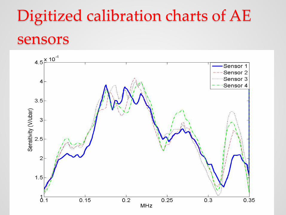
Digitized calibration charts of AE sensors

PLB test and system parameters determination

Averaged AEE responses of the PLB test at each cylinder

Averaged AEE responses of the PLB test at each cylinder

3D plot of evaluating the optimized attenuation and ATD parameters

Attenuation constant matrix and ATD matrix for the test engine, 𝜶𝜶 and 𝜷𝜷

An Example of AE signal Normalisation of Diesel Engine

Enlarged view of the combustion areas

Enlarged view of the combustion areas

Case study 2Green carbon mixer gearbox
D
EB H
CA

Bearing designations and defect frequencies
BPFI : Ball Passing Frequency on Inner raceBPFO : Ball Passing Frequency on Outer raceBSF : Ball Spin Frequency FTF : Fundamental Train Frequency

(B-1) Time wave form and power spectrum of AE and Acceleration signal from the point B.
0 2 4 6 8 10-10
-8
-6
-4
-2
0
2
4
6
8
Time (sec)
Ampl
itude
(mV)
Line3, Point B, AE, Data 3
RMS=0.340Crest F=9.286Kurtosis=7.467
0 2 4 6 8 10-1
-0.8
-0.6
-0.4
-0.2
0
0.2
0.4
0.6
0.8
Time (sec)
Acce
lerat
ion
(g)
Line3, Point B, ACC, Data 3
RMS=0.160Crest F=3.752Kurtosis=2.757
0 2 4 6 8 10x 104
10-3
10-2
10-1
100
101
102
Frequency (Hz)
Powe
r spe
ctru
m (m
Vrm
s2
)
Line 3,Point B, AE, Data 3
0 2 4 6 8 10x 104
10-4
10-3
10-2
10-1
100
101
102
103
Frequency (Hz)
Powe
r spe
ctru
m (g
rms
2)
Line 3,Point B, ACC, Data 3

(B-2) Envelope spectrum of AE
0 20 40 60 80 100 1200
0.2
0.4
0.6
0.8
1
1.2
1.4
Frequency (Hz)
Powe
r spe
ctru
m (µV
rms
2)
Line 3, Point B, AE30, HPF [4.5-10.5] kHz, 20-averaged envelop
←10.13 ←20.21
←30.34
←40.47 ←50.54
←60.68
←70.75 ←80.88 ←1.67
←91.02 ←101.09
←111.22 ←121.3 ←21.52 ← ←2.50 ←0.83
mPRO=13.32 dBmPRI=43.03 dB
0 20 40 60 80 100 1200
200
400
600
800
1000
1200
Frequency (Hz)
Powe
r spe
ctru
m (µV
rms
2)
Line 3, Point B, AE30, HPF [19.5-30.5] kHz, 20-averaged envelop
←1.67
←2.50 ←20.21 ←10.13
←30.34
←40.47 ←50.54 ←60.68
←70.75 ←0.83 ←80.88 ←91.02 ←101.09 ←4.17 ←21.52 ←111.22
mPRO=22.17 dBmPRI=43.69 dB
5-10kHz High Pass Filtering
20-30kHz High Pass Filtering
BPFO
BPFI

(E-1) Time wave form and power spectrum of AE and Acceleration signal from the point E.
0 2 4 6 8 10-6
-4
-2
0
2
4
6
8
Time (sec)
Ampl
itude
(mV)
Line3, Point E, AE, Data 3
RMS=0.281Crest F=9.656Kurtosis=5.933
0 2 4 6 8 10
-0.25
-0.2
-0.15
-0.1
-0.05
0
0.05
0.1
0.15
0.2
0.25
Time (sec)
Acce
lera
tion
(g)
Line3, Point E, ACC, Data 3
RMS=0.045Crest F=3.610Kurtosis=2.961
0 2 4 6 8 10x 104
10-3
10-2
10-1
100
101
102
Frequency (Hz)
Powe
r spe
ctru
m (m
Vrm
s2
)
Line 3,Point E, AE, Data 3
0 2 4 6 8 10x 104
10-6
10-4
10-2
100
102
Frequency (Hz)
Powe
r spe
ctru
m (g
rms
2)
Line 3,Point E, ACC, Data 3

(E-2) Envelope spectrum of AE
0 10 20 30 40 500
0.5
1
1.5
2
2.5
3
3.5
4
4.5 x 10⁻⁷
Frequency (Hz)
Powe
r spe
ctru
m ( µ
V rms
2)
Line 3, Point E, AE30, HPF [4.5-10.5] kHz, 20-averaged envelop
←10.20
←20.41
←30.61
←40.82
←1.62 ←0.86
←3.34 ←8.30 ←4.96 ←24.13
mPRO=48.93 dBmPRI=-0.13 dB
0 10 20 30 40 500
0.5
1
1.5
2
2.5
3
3.5 x 10⁻⁴
Frequency (Hz)
Powe
r spe
ctru
m ( µ
V rms
2)
Line 3, Point E, AE30, HPF [19.5-30.5] kHz, 20-averaged envelop
←10.20
←20.41
←30.61
←40.82
←1.62 ←2.48
←0.86 ←4.96 ←4.20 ←3.34
mPRO=50.83 dBmPRI=3.63 dB
5-10kHz High Pass Filtering
20-30kHz High Pass Filtering
BPFO
BPFI

Observations• AE energy is distributed within a range of frequency from
10 – 30 kHz, while as the acceleration decreases rapidly after 10 kHz.
• AE signals at points B and E (close to each other) show a series of impulsive impacts occurring at around 10 Hz.
• The enveloped spectrum of point E clearly show the 10 Hz component and its harmonics.
• Point B, close to Point E also detected the 10 Hz component and its harmonics, with smaller amplitudes.
• PHDS has successfully overcome to challenges of high sampling rate and massive data storage.
• Normalisation of multiple AE sensors has provides a clear comparison signal sensitivity and the data are presented in engineering unit rather than just in terms of voltage.