Acoustic Black Holesーブラックホール物理を実験室で検証するー

京都大学大学院　人間・環境学研究科

宇宙論・重力グループ　M2

奥住　聡

共同研究者：阪上雅昭（京大　人・環）, 吉田英生（京大　工）

Outline

1. Introduction: “What is an Acoustic Black Hole”?

2. “Acoustic BH Experiment Project”

3. Application I: Hawking Radiation (classical analogue)

4. Application II: Quasinormal Ringing

1.Introduction:

“What is an Acoustic Black Hole?”

Interest and Difficulty in Black Hole Physics

Black holes are the most fascinating objects in GR.Black holes are the most fascinating objects in GR.Black holes are the most fascinating objects in GR.Black holes are the most fascinating objects in GR.

Hawking radiation (quantum)

: thermal emission from BHs

Numerous quantum / classical phenomena have beenpredicted. For example,

Quasinormal Ringing (classical)

: characteristic oscillation of BHs

However, many of them are difficult to observe.

To examine them, an alternative way is nessesary!

What is an Acoustic Black Hole?

“Acoustic BH” = Transonic Flow

down 1−>M1−<M 1−=M up

sonic point

eff

sc

velocityfluid:

velocitysound:

v

cs)1(eff ±=±= Mccvc sss

“effective” sound velocity in the lab

Acoustic BH region

In the supersonic region,

sound waves cannot propagate against the flow

= sonic horizon

→　“Acoustic Black Hole”

0>+ scv0=+ scv0<+ scv

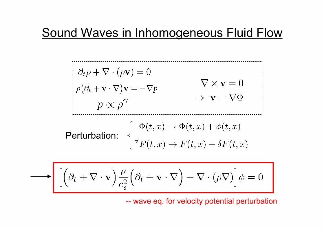
-- wave eq. for velocity potential perturbation

Sound Waves in Inhomogeneous Fluid Flow

Perturbation:

This is preciselypreciselypreciselyprecisely the eq. for a massless scalar fieldin a geometry with metric

[ ]ji

ij

ii

s

s

dxdxdtdxvdtcc

ds δρ

+−−−= 2)( 2222 v

,22dx

vc

vdtdT

s −+≡

( )2221

2

22

2

222 )1()1( dzdy

cdx

c

vdT

c

vc

cds

sss

s

s

++

−+−−= − ρρ

,)0,0,(v=v

Unruh, Phys. Rev. Lett. 46, 1351 (1981)

2~sd≡

“Acoustic Metric”: Metric for Sound Waves

Furthermore, setting

“Acoustic Metric”

21

2

222

2

22 )1()1(~ dx

c

vdTc

c

vsd

s

s

s

−−+−−= 21

2

2

ff22

2

2

ff2 )1()1(~ drc

vdtc

c

vsd S

−−+−−=

“Acoustic Metric” Schwarzschild Metric

sonic point horizon

“Acoustic Metric”: Metric for Sound WavesUnruh, Phys. Rev. Lett. 46, 1351 (1981)

coordinate axial:

velocityfluid:

sound of speed:

22

x

dxvc

vtT

v

c

s

s

∫ −+=

coordinate radial:

timeildSchwarzsch:

velocityfall-free:)/(

light of speed:

2/1

ff

r

t

rrcv

c

S

g−=

2. Acoustic BH Experiment Project:

Black Holes in Laval nozzles

throat

“Laval Nozzle”:Convergent-Divergent Nozzle

Two Types of Steady Flow in Laval Nozzles

flow flow

Pressure difference pu / pd determines the flow in the nozzle:

pupdthroat throat

Subsonic flow : max M at throat, but M<1 everywhere.

Transonic flow Transonic flow Transonic flow Transonic flow : M=1 at throat; supersonic region exists.(may have a steady shock downstream)

THEORY

Graduate School of H&E Studies

EXPERIMENT

Graduate School of Engineering

TARGETS

• Hawking Radiation

• Quasinormal Ringing

numerical

Planckian fit

Acoustic BH Experiment Project at Kyoto Univ.

compressor

mass flow meter

settling chamber

Laval nozzle

flow

20cm

Configuration

xb=8mm

throat

R=200mm

100mm 100mm

61.6mm 61.6mmx=0

Form of our Laval Nozzle

Preliminary Experiment:Acoustic Black Hole Formation

subsonicsubsonicsubsonicsubsonic transonictransonictransonictransonic

Acoustic BH is materialized in our experiments!!

3. Application I:

Classical Analogue of Hawking Radiation

Thermal emission from BHs.

Quantum phenomenon; derived from QFT in curved ST.( mixing of positive & negative freq. modes)

: “surface gravity”

Properties of Hawking Radiation

Too weak to observe in the case of astrophysical BHs!

How can we study Hawking Radiation?

Hawking radiation of phonon in airflow: impossible!!

(possible for BEC transonic flow ? [Garay et al., 2000] )

Nevertheless, some classical phenomena in acoustic BHs

will shed light on quantum aspects of Hawking radiation.

“classical counterpert of Hawking radiation”

Positive & Negative Frequency Mode Mixing

observer infinity

deformed

horizon

collapse

BH

positivepositivepositivepositive freq. mode(CLASSICAL)

surfacre gravity

exponential exponential exponential exponential redshiftredshiftredshiftredshift

Nonstationary evolution of ST � Change of vacuum state

star before collapse

negativenegativenegativenegative freq. part appears! Particle Creation!!quantization

Classical Counterpart of Hawking Radiation

Inner product (Fourier tr.):

Planck distribution!!

negativenegativenegativenegative freq. mode from infinity

positivepositivepositivepositive freq. mode for an observer

(Nouri-Zunoz & Padmanabhan, 1998)

Experimental Setting

Step 1: subsonic background flow ( no horizonno horizonno horizonno horizon ).Send sinusoidal sound wave against the flow.

Step 2: transonic background flow ( horizon presenthorizon presenthorizon presenthorizon present ).Observe the waveform at upstream region.

Redshift due to surface gravityincident freq:15kHz

horizon formed

Numerical Waveform (quasi-stationary flow, geometric acoustics limit)

Redshift due to surface gravityincident freq:15kHz

horizon formed

Numerical Waveform (quasi-stationary flow, geometric acoustics limit)

sinusoidal wave(t<0)

(next slide)

incident freq:15kHz

Numerical Spectrum(quasi-stationary flow, geometric acoustics limit)

Numerical Spectrum(quasi-stationary flow, geometric acoustics limit)

penetrates into positive frequency range!

(next slide)

Numerical Spectrum(quasi-stationary flow, geometric acoustics limit)

500 1000 1500 2000 2500 3000

f@HzD

1 ´ 10- 7

2 ´ 10- 7

3 ´ 10- 7

4 ´ 10- 7

5 ´ 10- 7

SHfL

500 1000 1500 2000 2500 3000

f Hz

1ｴ10- 7

2ｴ10- 7

3ｴ10- 7

4ｴ10- 7

5ｴ10- 7

S

Planckian fit

1)exp(2 −∝

κπω

ω

Numerical

Observation in a Laboratory

Signal is buried in noise.

However, output of LIA implies that redshift occurs.

Classical Counterpart of HR: Discussion

Recently, full order calculation has been performed.

Furuhashi, Nambu and Saida, CQG 23, 5417 (2006)

Their results agree with our calculation.

Planckian distr. seems to be robust.

Does the thermal emission of phonon really occur

in quantum fluids (BEC / superfluid) ?

How about the effect of high frequency dispersion?

3. Application II:

Quasinormal Ringing

Okuzumi & Sakagami

“Quasionormal Ringing of Acoustic Black Holes in Laval Nozzles”

in preparation

Quasinormal Ringing

“Characteristic ‘sound’of BHs (and NSs)”

Arises when the geometry around a BH is perturbed and settles down into its stationary state.

e.g. after BH formation / test particle infall

Described as a superposition of a countably infinite number

of damped sinusoids (QuasiNormal QuasiNormal QuasiNormal QuasiNormal Modes, Modes, Modes, Modes, QNMsQNMsQNMsQNMs).

QNM frequencies contain the information on (M,J) of BHs.

Quasinormal Ringing of a BH

NS-NS marger to a BH (Shibata & Taniguchi, 2006)

QN ringing

inspiral phase marger phase

Mathematical Description of QNMs

Schrodinger-type Eq. outgoing B.C.with..

In general, QNMs are defined as solutions of

V(ξ): effective potential barrier

Examples of Schroedinger-type Equation

(1) Schwarzschild Black Hole

Examples of Schroedinger-type Equation

(1) Schwarzschild Black Hole

horizon spatial infinity

Examples of Schroedinger-type Equation

(2) Acoustic Black Hole in a Laval Nozzle

cs0: sound speed at stagnation points

Potential Barrier for Different Laval Nozzles

Consider two-parameter family of Laval nozzle.

nozzle radius

: radius of the throat

K : integer

1.0

tank 1 tank 2nozzleflow

Potential Barrier for Different Laval Nozzles

1.04

3.92

11.4

1.19

flow

sonic horizon

flow

sonic horizon

QNM Frequencies of Different Laval Nozzle(the least-damped (n=0) mode; 3rd WKB value)

easier to observe

Re/Im ~ 4

(WKB approx.is not good)

Numerical Simulation of Acoustic QN Ringing

We perform two types of simulations:

“Acoustic BH Formation”

initial state: no flowset sufficiently largepressure difference

final state: transonic flow

“Weak Shock Infall”

initial state: transonic flow‘shoot’ a weak shock into the flow

final state: transonic flow

~ BH formation ~ test particle infall

Example of Transonic Flow

flow

sonic horizonsupersonic subsonic

Result 1: Weak Shock Infall

steady shock

horizon

weak shock

QN ringing

gif

QNM fitnumerical

nonlinear phase ringdown phase

Result 2: Acoustic BH Formation

observed waveform

QNM fitnumerical

nonlinear phase ringdown phase

Result 2: Acoustic BH Formation

observed waveform

Numerical Simulation: Summary

In both types of simulations, QNMs are actually excited.

The results agree with WKB analysis well ( for K >1 ).

cf. Schwarzschild, l = 2 , least-damped mode

Typical values in laboratories:

� similar to values for astrophysical BHs

Numerical Simulation: Discussion

For future experiments, larger Q-value is wanted.

However, Q is at most ~ 2 for planar wave modes.

QNMs of an Acoustic BH surrounded by a “half-mirror”(contact surface)

QNMs for non-planar waves

Can matched filtering be used in our experiments ?

Summary

“Acoustic BH” = Transonic Flow

wave eq. for sound in perfect fluid

� wawe eq. for a massless scalar field in curved ST

sonic point � event horizon of a BH

Results of numerical simulations strongly suggest

that classical counterpart of HR and QN ringing

can be realized in a laboratory.

Appendix

Standard Procedure for Calculating QNM Freq’s

Calculate the “S-matrix” for the potential barrier V(ξ):

Then, impose the outgoing B.C. , and obtain κ ’s that meet the boundary condition.

: “S-matrix”

WKB Approach

ξ0

κ2

Region (I) & (III): WKB solutions for truncated V(ξ)Around ξ0 : exact solution for truncated V(ξ)

Expand V(ξ) in a Taylor series about the maximum point ξ0:

(I) (II) (III)

1st order: Schutz & Will, 1985

3rd order: Iyer & Will, 1987

6th order: Konoplya, 2004

MatchingMatchingMatchingMatching

matching regionsmatching regionsmatching regionsmatching regions

ξ23ξ12

WKB Approach: S-Matrix

Here, Here, Here, Here, νννν is related to is related to is related to is related to κκκκ by by by by

where

(1st WKB)

QNM Solutions by WKB Approach

Conditions for QNMs:

i.e.

QNM frequencyQNM frequencyQNM frequencyQNM frequency(1st WKB value)

Partially Reflected Quasinormal Modes(PRQNMs)

outgoing B.C. + ““““half mirrorhalf mirrorhalf mirrorhalf mirror”””” B.C.B.C.B.C.B.C.

“half mirrorhalf mirrorhalf mirrorhalf mirror”

ξc

Example: Contact Surface in Perfect Fluid

Contact surfaceContact surfaceContact surfaceContact surface (contact discontinuity):• discontinuity of the density ρ .• the pressure p and the fluid velocity v are continuous.• moves with the surrounding fluid, i.e., vc= v .• partially reflects sound waves.

vcv v

1 2

Contact Surface

(C.S.)

Example: Contact Surface in Perfect Fluid

vcv v

1 2

If vc(= v) << cs ,refl. coeff. R(κ) for sound waves propagating from 1 to 2is given by [e.g. Landau & Lifshitz, Fluid Mechanics]

C.S.

PRQNM Solutions by WKB ApproachIn region (III),

right-going WKB sol. left-going WKB sol.

ξc

region (III) region (IV)

ξ23

PRQNM Solutions by WKB ApproachIn region (III),

right-going WKB sol. left-going WKB sol.

Furthermore, if ξc lies far away from the potential barrier,

PRQNM Solutions by WKB Approach

Partially Reflecting B.C. :

PRQNM frequency:

Example: Contact Surface in Perfect Fluid

Re ReIm Im

TableTableTableTable: the least damped PRQNM for an acoustic BH

QNM fit

PRQNM fit

Numerical Simulation of PRQNMs

For t <15, an “ordinary” QNM (notnotnotnot PRQNM) dominates,since the potential barrier is not yet “aware”of the contact surface.