Embed Size (px)
Citation preview

Jean-Pierre GattusoLaboratoire dʼOcéanographie de Villefranche
CNRS-Université Pierre et Marie Curie
Acidification de lʼocéan et son impact sur les organismes et écosystèmes marins

http://epoca-project.eu
Une thématique de recherche récente
10/01/2005 09:47 AMOcean Acidification Bad for Shells and Reefs -- Parks 2005 (928): 5 -- sciencenow
Page 1 of 2http://sciencenow.sciencemag.org/cgi/content/full/2005/928/5
Gassed. Skeleton-building fellby 50 percent in corals studiedin this gutterlike flume whencarbon dioxide was doubled.
JEAN-PIERRE GATTUSO | Change Password | Change User Information | Access Rights |
Subscription HELP | Sign Out
28
September
2005
Ocean Acidification Bad for Shells and Reefs
Rising levels of atmospheric carbon due to fossil fuel emissions have made seawater
more acidic. Now, two new studies show that increasing acidification could wreak
havoc on marine organisms that build their shells and skeletons from calcium
carbonate. Since these creatures provide essential food and habitat for other ocean
dwellers, the effects could ripple disastrously throughout the ocean, the researchers
warn.
Greenhouse gasses such as carbon dioxide
are changing the oceans in many ways,
such as warming the water. Marine
creatures could get another shock as the
ocean absorbs ever-greater quantities of
the gas--expected to rise two to three
times over pre-industrial levels during the
next 50 to 100 years. This will create more
acidic conditions in the sea that diminish
the concentration of carbonate needed for
shell and skeleton building.
To study the potential impact, a team of
27 marine chemists and biologists
combined the latest measurements on
ocean carbon with 13 global carbon
models. The models project that polar
waters will begin dissolving shells and
other calcified materials when atmospheric
CO2 reaches 600 parts per million, which
could occur within several decades.
Experiments with live pteropods--
swimming snails consumed by fish and
whales--exposed to sea water of the pH
predicted for year 2100 showed that the
creatures' shells began to dissolve after
two days. "Unlike climate predictions, the
uncertainties here are small," says lead
author James Orr, of the French
Laboratoire des Sciences du Climat et de

http://epoca-project.eu
Une thématique de recherche récente

• CO2 emissions:• 1990-1999 : +1% per year• 2000-2007 : +3.4% per year
What is the cause of OA?

• CO2 emissions:• 1990-1999 : +1% per year• 2000-2007 : +3.4% per year
What is the cause of OA?
NATURE GEOSCIENCE | ADVANCE ONLINE PUBLICATION | www.nature.com/naturegeoscience 1
correspondence
To the Editor — Emissions of CO2 are the main contributor to anthropogenic climate change. Here we present updated information on their present and near-future estimates. We calculate that global CO2 emissions from fossil fuel burning decreased by 1.3% in 2009 owing to the global !nancial and economic crisis that started in 2008; this is half the decrease anticipated a year ago1. If economic growth proceeds as expected2, emissions are projected to increase by more than 3% in 2010, approaching the high emissions growth rates that were observed from 2000 to 20081,3,4. We estimate that recent CO2 emissions from deforestation and other land-use changes (LUCs) have declined compared with the 1990s, primarily because of reduced rates of deforestation in the tropics5 and a smaller contribution owing to forest regrowth elsewhere.
Fossil fuel CO2 emissions for the globe are computed from statistics on energy consumption at the country level6,7 and converted to CO2 emissions by fuel type8. "e growth in CO2 emissions closely follows the growth in Gross Domestic Product (GDP) corrected for improvements in energy e#ciency4. "us, the contraction of GDP owing to the global !nancial crisis that began in 2008 was expected to cause a decrease in global CO2 emissions. Emissions in 2008 grew at a similar rate to the previous eight years, but they decreased by 1.3% in 2009. Despite this drop, the 2009 global fossil fuel and cement emissions were the second highest in human history at 8.4 ± 0.5 Pg C (30.8 billion tons of CO2), just below the 2008 emissions7.
"is global decrease hides large regional di$erences. "e largest decreases occurred in Europe, Japan and North America (for example, USA %6.9%, UK %8.6%, Germany %7%, Japan %11.8%, Russia %8.4%), whereas some emerging economies recorded substantial increases in their total emissions (for example, China +8%, India +6.2%, South Korea +1.4%).
"e observed decrease of 1.3% in global fossil fuel emissions in 2009 is less than half of the decrease of 2.8% projected a year ago1. "at projection used a forecast from the International Monetary Fund for the annual real growth in world GDP2 and assumed that the carbon intensity of world GDP (that is, the fossil fuel emissions per unit of GDP) would continue to improve following a
long-term trend reduction of carbon intensity of %1.7% yr%1. "e decrease in emissions was lower than projected for two reasons. First, the actual decrease2 in GDP (%0.6%) was lower than forecast in October 2009 (%1.1%) because of continuing high GDP growth in China (+9.1%) and other emerging economies. Second, the carbon intensity of world GDP improved by only %0.7% in 2009, less than half of its long-term average, because of an increased share of fossil fuel CO2 emissions coming from emerging economies with a relatively high carbon intensity and an increasing reliance on coal. Both globally and for emerging economies, the fraction of fossil fuel emissions from coal increased in 2009, as in 20081.
As the global economy recovers, the world GDP is projected to increase by 4.8% in 20102. Even if the carbon intensity of world GDP improves following its long-term average, global emissions will have increased again by more than 3% in 2010 (Fig. 1).
Historical CO2 emissions from LUC were revised and updated to 2009 using new data on forest cover and land use — reported by each country and compiled by the Food and Agricultural Organization5 — and a LUC emission model9. "e estimate of average 2000 to 2009 LUC emissions of 1.1 ± 0.7 Pg C yr%1 has been revised downwards from the estimate that was made in 20091 (Fig. 1), primarily because of a downward revision of the rates of deforestation in tropical Asia. LUC emissions for the past decade are now lower than their 1990s level (1.5 ± 0.7 Pg C yr%1), although the decadal di$erence is still below the uncertainty in the data and method. A recent decrease in LUC emissions would be consistent with the reported downward trends of deforestation detected from satellite data in the Brazilian Amazon10 and Indonesia11. Temperate forest regrowth in Eurasia has constantly increased since the 1950s at a rate of 0.2 Pg C yr%1 per decade. For the !rst time, according to our estimate, forest regrowth has overcompensated LUC emissions at temperate latitudes and has resulted in a small net sink of CO2 (< 0.1 Pg C yr%1) since 2000 in these latitudes.
Atmospheric CO2 continued to increase, reaching a globally averaged concentration of 387.2 ppm at the end of 200912. "e increase in atmospheric CO2 of 3.4 ± 0.1 Pg C yr%1 was among the lowest since 2000. "is cannot be explained by
the decrease in CO2 emissions alone but is mainly caused by an increase in the land and ocean CO2 sinks in response to the tail of the La Niña event that perturbed the global climate system from mid 2007 until early 2009.
References1. Le Quéré, C. et al. Nature Geosci. 2, 831–836 (2009). 2. World Economy Outlook Update (International Monetary Fund,
2010); http://go.nature.com/ttuu5K3. Canadell, J. G. et al. Proc. Natl Acad. Sci. USA
104, 18866–18870 (2007).4. Raupach, M. R. et al. Proc. Natl Acad. Sci. USA
104, 9913–9914 (2007).5. Global Forest Resources Assessment 2010 (Food and Agriculture
Organization of the United Nations, 2010); http://www.fao.org/forestry/fra/fra2010/en/
6. http://go.nature.com/otKuy9
Update on CO2 emissions
Fossil fueland cement
LUC
9
8
7
2
1
0 2000 2005 2010Time (yr)
2000 2005 2010Time (yr)
30
25
10
5
0
CO2
emissions (billion tons CO
2 yr –1)CO
2 em
issions (billion tons CO2 yr –1)
CO2 e
miss
ions
(Pg
C yr
–1)
CO2 e
miss
ions
(Pg
C yr
–1)
Figure 1 | Global CO2 emissions since 1997 from fossil fuel and cement production (a) and LUC (b). Fossil fuel CO2 emissions were based on United Nations Energy Statistics to 2007, and on BP energy data from 2007 onwards6,7. Cement CO2 emissions are from the US Geological Survey. LUC CO2 emissions were based on the revised statistics of the Food and Agricultural Organization5,9. Both sources of emissions are updated from ref. 1 (shown in black dashed line). Projections for 2010 are included in red.
http://epoca-project.eu
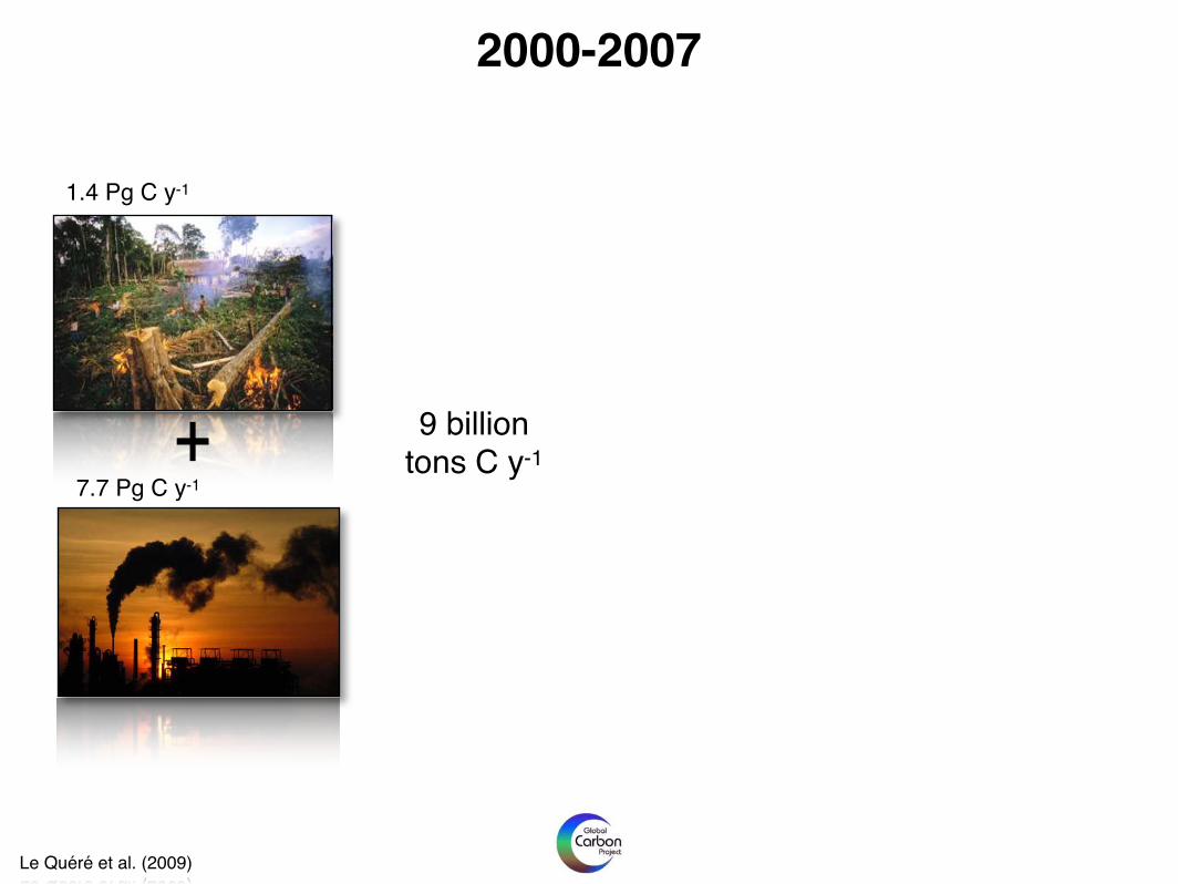
Le Quéré et al. (2009)
1.4 Pg C y-1
+7.7 Pg C y-1
2000-2007
9 billion tons C y-1

http://epoca-project.eu
Le Quéré et al. (2009)
1.4 Pg C y-1
+7.7 Pg C y-1
2000-2007
Atmosphere45%
4.1 Pg y-1
Vegetation29%
2.7 Pg y-1
Oceans26%
2.3 Pg y-1 24 millions tonnes CO2 per day
9 billion tons C y-1

http://epoca-project.eu
Sabine et al. (2004)
because of the substantially higher verticallyintegrated concentrations and the large oceanarea in these latitude bands (Fig. 1, table S1).About 60% of the total oceanic anthropogen-ic CO2 inventory is stored in the SouthernHemisphere oceans, roughly in proportion tothe larger ocean area of this hemisphere.
Figure 2 shows the anthropogenic CO2
distributions along representative meridi-onal sections in the Atlantic, Pacific, andIndian oceans for the mid-1990s. Becauseanthropogenic CO2 invades the ocean bygas exchange across the air-sea interface,the highest concentrations of anthropogenicCO2 are found in near-surface waters.Away from deep water formation regions,the time scales for mixing of near-surfacewaters downward into the deep ocean canbe centuries, and as of the mid-1990s, the
anthropogenic CO2 concentration in mostof the deep ocean remained below the de-tection limit for the !C* technique.
Variations in surface concentrations are re-lated to the length of time that the waters havebeen exposed to the atmosphere and to thebuffer capacity, or Revelle factor, for seawater(12, 13). This factor describes how the partialpressure of CO2 in seawater (PCO2) changes fora given change in DIC. Its value is proportionalto the ratio between DIC and alkalinity, wherethe latter term describes the oceanic chargebalance. Low Revelle factors are generallyfound in the warm tropical and subtropical wa-ters, and high Revelle factors are found in thecold high latitude waters (Fig. 3). The capacityfor ocean waters to take up anthropogenic CO2
from the atmosphere is inversely proportionalto the value of the Revelle factor; hence, the
lower the Revelle factor, the higher the oceanicequilibrium concentration of anthropogenicCO2 for a given atmospheric CO2 perturbation.The highest anthropogenic CO2 concentrations("60 #mol kg$1) are found in the subtropicalAtlantic surface waters because of the low Rev-elle factors in that region. By contrast, the near-surface waters of the North Pacific have a high-er Revelle factor at comparable latitudes andconsequently lower anthropogenic CO2 con-centrations primarily because North Pacific al-kalinity values are as much as 100 #mol kg$1
lower than those in the North Atlantic (Fig. 3).About 30% of the anthropogenic CO2 is
found at depths shallower than 200 m andnearly 50% at depths above 400 m. Theglobal average depth of the 5 #mol kg$1
contour is "1000 m. The majority of theanthropogenic CO2 in the ocean is, therefore,confined to the thermocline, i.e., the region ofthe upper ocean where temperature changesrapidly with depth. Variations in the penetra-tion depth of anthropogenic CO2 are deter-mined by how rapidly the anthropogenic CO2
that has accumulated in the near-surface wa-ters is transported into the ocean interior. Thistransport occurs primarily along surfaces ofconstant density called isopycnal surfaces.
The deepest penetrations are associatedwith convergence zones at temperate lati-tudes where water that has recently been incontact with the atmosphere can be transport-ed into the ocean interior. The isopycnal sur-faces in these regions tend to be thick andinclined, providing a pathway for the move-ment of anthropogenic CO2-laden waters intothe ocean interior. Low vertical penetration isgenerally observed in regions of upwelling,such as the Equatorial Pacific, where inter-mediate-depth waters, low in anthropogenicCO2, are transported toward the surface. Theisopycnal layers in the tropical thermoclinetend to be shallow and thin, minimizing themovement of anthropogenic CO2-laden wa-ters into the ocean interior.
Figure 4A shows the distribution of an-thropogenic CO2 on a relatively shallowisopycnal surface (see depths in Fig. 2) witha potential density (%&) of 26.0. About 20%of the anthropogenic CO2 is stored in waterswith potential densities equal to or less thanthat of this surface. The highest concentra-tions are generally found closest to where thisdensity intersects the surface, an area referredto as the outcrop. Concentrations decreaseaway from these outcrops in the Indian andPacific oceans, primarily reflecting the aging ofthese waters, i.e., these waters were exposed tolower atmospheric CO2 concentrations whenthey were last in contact with the atmosphere.The Atlantic waters do not show this trendbecause the 26.0 %& surface is much shallowerand therefore relatively well connected to theventilated surface waters throughout most ofthe Atlantic (Figs. 2A and 4A).
Fig. 2. Representative sections of anthropogenic CO2 (#mol kg$1) from (A) the Atlantic, (B) Pacific, and
Indian (C) oceans. Gray hatched regions and numbers indicate distribution of intermediate water masses(and North Atlantic DeepWater) on the given section and the total inventory of anthropogenic CO2 (PgC) within these water masses. The southern water masses in each ocean represent Antarctic Interme-diate Water. The northern water masses represent the North Atlantic Deep Water (A), North PacificIntermediate Water (B), and Red Sea/Persian Gulf Intermediate Water (C). The two bold lines in eachpanel give the potential density [%& ' (density – 1)( 1000] contours for the surfaces shown in Fig. 4.Insets show maps of the cruise tracks used. Note that the depth scale for (A) is twice that of the otherfigures, reflecting the deeper penetration in the North Atlantic.
R E S E A R C H A R T I C L E S
16 JULY 2004 VOL 305 SCIENCE www.sciencemag.org368
CO2 invasion

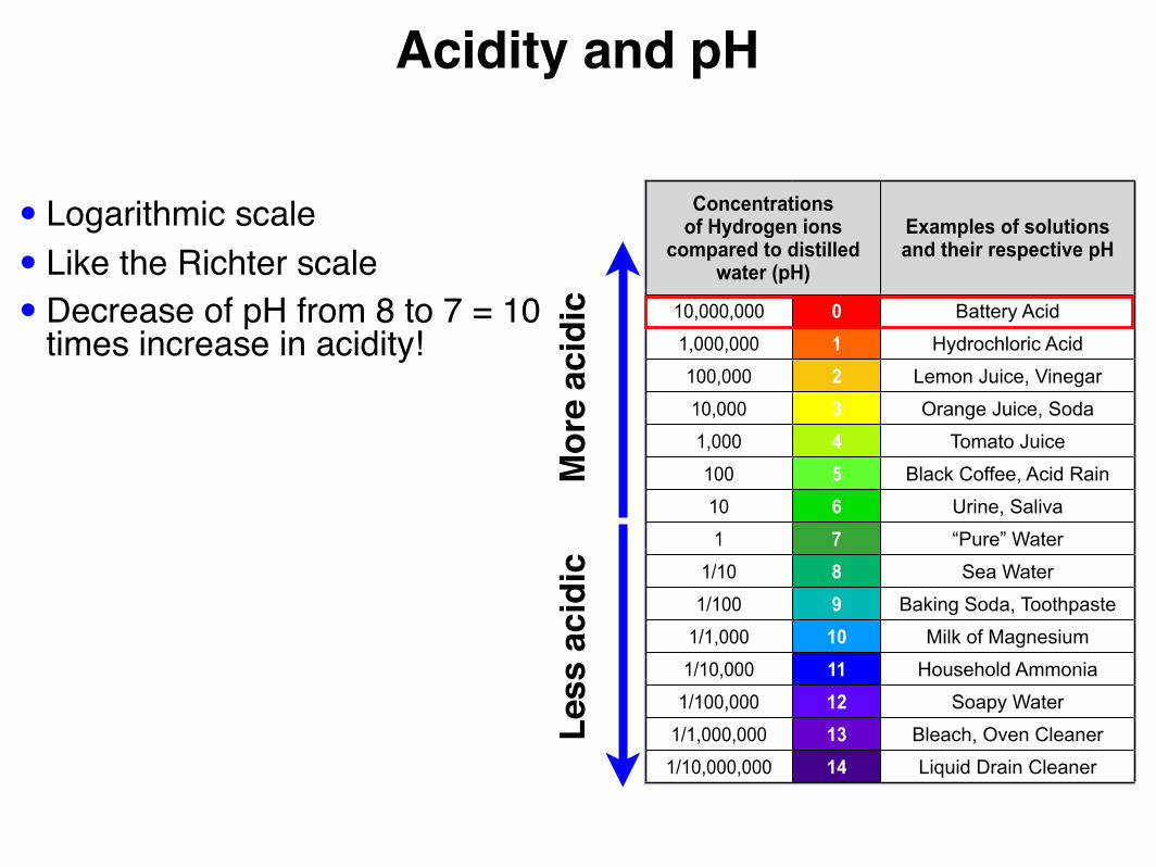
Acidity and pH
• Logarithmic scale• Like the Richter scale• Decrease of pH from 8 to 7 = 10
times increase in acidity!
Mor
e ac
idic
Less
aci
dic

Concentrations of Hydrogen ions
compared to distilled water (pH)
Examples of solutions and their respective pH
10,000,000 0 Battery Acid
1,000,000 1 Hydrochloric Acid
100,000 2 Lemon Juice, Vinegar
10,000 3 Orange Juice, Soda
1,000 4 Tomato Juice
100 5 Black Coffee, Acid Rain
10 6 Urine, Saliva
1 7 “Pure” Water
1/10 8 Sea Water
1/100 9 Baking Soda, Toothpaste
1/1,000 10 Milk of Magnesium
1/10,000 11 Household Ammonia
1/100,000 12 Soapy Water
1/1,000,000 13 Bleach, Oven Cleaner
1/10,000,000 14 Liquid Drain Cleaner
Acidity and pH
• Logarithmic scale• Like the Richter scale• Decrease of pH from 8 to 7 = 10
times increase in acidity!
Mor
e ac
idic
Less
aci
dic

http://epoca-project.eu
What is ocean acidification?Increased
CO2
Decreasedcarbonate
Increasedbicarbonate

http://epoca-project.eu
What is ocean acidification?
Acidity increases:“ocean acidification”
IncreasedCO2
Decreasedcarbonate
Increasedbicarbonate
Hydrogen ion concentration increases
and pH decreases
HCO−3
K2� CO2−3 + 2H+
K2 is a dissociation constant of carbonic acid:
K∗2 =
[CO2−3 ][H+]
[HCO−3 ]
hence [H+] = K∗2[HCO−
3 ]
[CO2−3 ]
1

http://epoca-project.eu
What is ocean acidification?
69
16
1800 2000 2100
Acidity : x 10-9 mol H+ kg-1
8.2
8.1
7.8
1800 2000 2100
+ 34%
+ 152%
http://epoca-project.eu
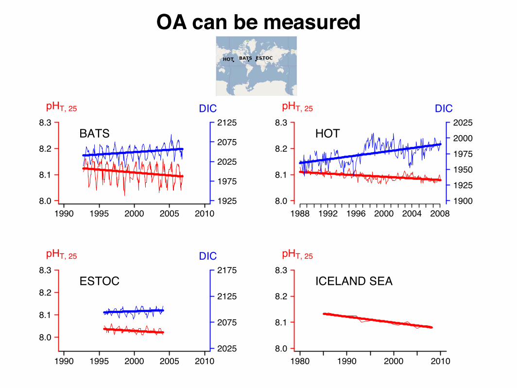
OA can be measured
BATS
1990 1995 2000 2005 20108.0
8.1
8.2
8.3
pHT, 25 DIC
1925
1975
2025
2075
2125HOT
1988 1992 1996 2000 2004 20088.0
8.1
8.2
8.3
pHT, 25 DIC
190019251950197520002025
1990 1995 2000 2005 2010
8.0
8.1
8.2
8.3
pHT, 25 DIC
2025
2075
2125
2175ESTOC
1980 1990 2000 20108.0
8.1
8.2
8.3
pHT, 25
ICELAND SEA

http://epoca-project.eu
Research projects
Ocean acidification research and its international coordination and dissemination: a three-year funding proposal ($1.755m)
Jean-Pierre Gattuso1 and members of the SIOA WGDan Laffoley2 and members of the IOA RUG
22 February 2011
The proposalProfound changes in seawater chemistry are underway as the ocean takes up about one fourth of the anthropogenic CO2 emitted to the atmosphere year-on-year. As this uptake continues into the future, further changes in ocean chemistry will occur, driving concern for marine organisms, ecosystems, and policy issues.
As national research activities on ocean acidification emerge world wide (Figure 1), it is crucial to coordinate the key overarching activities, at an international level, to generate a comprehensive understanding of the global effects of ocean acidification, and also for timely integration with policy advice and action. Such coordination would facilitate sharing of know-how, equipment, and joint experiments while avoiding excessive redundancy. This issue has been considered in depth over the last six months by the SOLAS-IMBER Ocean Acidification Working Group (SIOA WG) in concert with other major players, including the International Reference User Group on Ocean Acidification. The SIOA WG consists of representatives from the world’s major ocean acidification research programmes currently underway in in Australia, China, France, Germany, Japan, UK and USA.
The SIOA WG recently met in Washington with all major US funding agencies. Following these discussions and in partnership with the International Reference User Group on Ocean Acidification, it is unanimously recommended that an “Ocean Acidification International Coordination Office (OA-ICO)” be established to serve the needs of the research community and stakeholders. The task of the OA-ICO would be to implement the key overarching activities that must be performed at the international level to make effective use of the science investment. Once in operation the OA-ICO would replace the SIOA WG, which would then be used as the basis for the Advisory board of the International Coordination Office. The new OA-ICO would also form the core of the Monaco Ocean Acidification Action Plan3 to scale up global actions on ocean acidification. This international initiative is supported by a large number of national projects (Appendix 1), as well as by key organisations, including IOC-UNESCO, SCOR, and SOLAS and IMBER, two program elements of IGBP.
The core work of the OA-ICO would consist of a defined package of focused international activities which are not currently funded at national or international levels. These are described in the following pages under the headings of (1) structure of the OA-ICO office, (2) international coordination of research activities (ten actions outlined), and (3) international dissemination activities (two actions outlined).
1 Chair, SOLAS-IMBER Working Group on Ocean Acidification (see Appendix 1)2 Chair, International Ocean Acidification Reference User Group (see Appendix 2)3 In prep. stemming from the International Ocean Acidification RUG meeting in Monaco, November 2010
In less than a decade ocean acidification has emerged as a key issue of global concern. Levering the greatest value out of national research programme investments, and enabling coordinated international effort is now the key priority worldwide. This brief paper sets out the new core of international activity needed to scale up, support and enable our understanding of ocean acidification. It has been brought together by the key players in the international community acting as a single voice on what needs to be achieved, drawing from global experience and best practice.
Figure 1: Major ocean acidification research programmes around the world in 2011 (Courtesy Keizer et al., PML).

http://epoca-project.eu
Considerable increase in research efforts
Gattuso & Hansson (in press); Gattuso et al. (in press)
Year
Pape
rs p
ublis
hed
each
yea
r
0
50
100
150
200
250
● ●●●● ●● ●●● ● ●●●●● ●●●●●●●●●●●●●●●●●●●
●●●●●●
●●●●●
●●
●
●
●
●
●
1920 1940 1960 1980 2000Year
Num
ber o
f aut
hors
eac
h ye
ar
0
100
200
300
400
500
600
● ●●●● ●●● ●●● ● ●●●●● ●●●●●●●●●●●●●●●●
●●
●
●●
●
●
●
●●●●●
●
●
●
●
●
●
●
1920 1940 1960 1980 2000

Biological response: meta-analyses

Biological response: meta-analyses
• Hendriks & Duarte (2010): ... limited impact of experimental acidification on organism processes... except on calcification
• Kroeker et al. (2010): ... biological effects of ocean acidification are generally large and negative...
• Liu et al. (2010): This review and analysis ... suggest that ... the rates of several (microbial) processes will be affected by ocean acidification, some positively (N2 fixation...), others negatively.

OA: knowns, unknowns and perspectives1. Ocean acidification: background and history (Gattuso &
Hansson)2. Past changes of ocean carbonate chemistry (Zeebe &
Ridgwell)3. Recent and future changes in ocean carbonate chemistry
(Orr)4. Skeletons and ocean chemistry: the long view (Knoll &
Fischer) 5. Effect of ocean acidification on the diversity and activity of
heterotrophic marine microorganisms (Weinbauer et al.)6. Effects of ocean acidification on pelagic organisms and
ecosystems (Riebesell & Tortell)7. Effects of ocean acidification on benthic processes,
organisms, and ecosystems (Andersson et al.)8. Effects of ocean acidification on nektonic organisms
(Pörtner et al.)9. Effects of ocean acidification on sediment fauna
(Widdicombe et al.)10.Effects of ocean acidification on marine biodiversity and ec
osystem function (Barry et al.) 11.Effects of ocean acidification on the marine source of
atmospherically-active trace gases (Hopkins et al.)12.Biogeochemical consequences of ocean acidification and
feedback to the Earth system (Gehlen et al.) 13.The ocean acidification challenges facing science and
society (Turley & Kelvin) 14.Impact of climate change mitigation on ocean acidification
projections (Joos et al.)15.Ocean acidification: knowns, unknowns and perspectives
(Gattuso et al.)
ocean acidificationJean-Pierre Gattuso and Lina Hansson
B IOLOGY
Oxford University Press, September 2011
http://epoca-project.eu
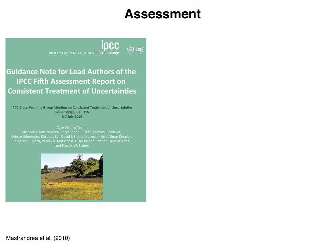
Assessment
!"#$%&'()*+,()-+.)/(%$)0",1+.2)+-),1()
345)6"78)9:;:
!
Mastrandrea et al. (2010)

http://epoca-project.eu
Assessment
!"#$%&'()*+,()-+.)/(%$)0",1+.2)+-),1()
345)6"78)9:;:
!
Mastrandrea et al. (2010)
Very low Low Medium High Very high
Limited
Medium
Robust
Level of confidence
Leve
l of e
vide
nce

http://epoca-project.eu
Assessment
VL L M H VH
L
M
R
Confidence
Evid
ence
!"#$%&'()*+,()-+.)/(%$)0",1+.2)+-),1()
345)6"78)9:;:
!
Mastrandrea et al. (2010)
Very low Low Medium High Very high
Limited
Medium
Robust
Level of confidence
Leve
l of e
vide
nce

http://epoca-project.eu
Assessment
VL L M H VH
L
M
R
Confidence
Evid
ence
!"#$%&'()*+,()-+.)/(%$)0",1+.2)+-),1()
345)6"78)9:;:
!
Mastrandrea et al. (2010)
Very low Low Medium High Very high
Limited
Medium
Robust
Level of confidence
Leve
l of e
vide
nce
15 declarative statements assessed:• Chemical aspects• Biological and biogeochemical responses• Policy and socio-economic aspects

http://epoca-project.eu
OA occurred in the past
VL L M H VH
L
M
R
Confidence
Evid
ence
Zeebe & Ridgwell (in press); Gattuso et al. (in press)
Challenge:Better constrain paleo-reconstructions of the carbonate system

http://epoca-project.eu
OA is in progress
VL L M H VH
L
M
R
Confidence
Evid
ence
Orr (in press); Gattuso et al. (in press)
Challenge:Better monitoring of key areas (e.g., coastal sites, coral reefs, polar regions and the deep sea)
Year
pC
O2 (µ
atm
)
280
300
320
340
360
380
400
420
!
!
!!!
!
!
!
!!
!
!!!
!!
!
!
!
!
!
!
!
!
!
!
!
!
!
!
!!
!!!
!!
!
!
!!
!
!!
!
!
!
!
!
!!
!
!
!!
!
!
!
!!
!
!
!
!
!
!!!
!
!
!
!!
!
!
!
!!
!!
!
!
!
!
!
!
!
!
!!
!
!!
!
!
!
!
!
!
!
!
!!
!
!!!!
!
!
!
!
!
!!
!
!
!!
!!
!
!
!!
!
!
!!
!
!
!!!
!
!
!
!
!!
!
!
!
!
!!
!!
!!
!
!
!!!
!
!
!
!
!!
!!
!
!!
!
!
!
!!
!!
!!
!!!
!!
!
!
!
!
!
!
!!
!
!
!
!
!
!
!
!
!
!
!
!
!
!
!!
!
!!
!
!
!
!
!
!
!
!
!
!
!
!
!
!
!!
!
!
!
!!
!
!
!
!
!
!
!
!
!
!
!!
!
!
!
!
!
!
!
!
!
!
!
!
!
!
!
!
!
!
!
!
!
!!!!
!
!
!!
!
!!
!!
1985 1990 1995 2000 2005
Year
pH
T
8.05
8.10
8.15
!
!
!!!
!
!
!
!!
!
!!!
!!
!
!
!
!
!!
!
!
!
!
!
!
!
!
!!
!!!
!!
!
!
!!
!
!!
!
!
!
!
!
!!
!!
!!
!
!
!
!!
!
!
!!
!
!!!
!
!
!
!!
!
!
!
!!
!!
!
!
!
!
!
!
!
!
!!
!
!!
!
!
!
!
!
!
!
!
!!
!
!!!!
!
!
!
!
!
!
!
!
!!!
!!
!
!
!!
!
!
!!
!
!
!!!
!
!
!
!
!!
!
!
!
!
!!!!
!!
!
!
!!!
!
!
!
!
!!
!!
!
!!
!
!!
!!
!!
!!
!!!
!!
!
!
!
!
!
!
!!
!
!
!
!
!
!
!
!
!
!
!
!
!
!
!!
!
!
!
!
!
!
!
!
!
!
!
!
!
!
!
!
!
!!
!
!
!
!!
!
!
!
!
!
!
!
!
!
!
!!
!
!!
!
!
!
!!
!
!
!
!
!
!
!
!
!
!
!
!
!
!!!!
!
!
!!
!
!!
!!
1985 1990 1995 2000 2005
Year
[CO
32!] (µ
mol kg!1)
220
230
240
250
260
!!
!
!!
!!!
!
!
!
!
!!
!
!!
!
!
!
!
!!
!
!!
!!
!!
!
!
!
!
!
!
!
!!
!
!
!
!
!!
!
!
!
!
!
!
!
!
!
!
!
!!
!
!
!
!
!
!!
!
!
!
!
!
!
!
!
!!!!
!
!
!
!
!
!!
!
!
!!
!
!
!
!
!
!
!
!
!!!
!!!
!
!
!
!!
!!
!!
!
!!
!!
!
!
!
!
!
!
!
!!
!!!!
!
!!!
!!
!
!
!
!
!!
!
!
!
!
!
!!
!
!
!!!
!!!
!
!
!
!
!
!!
!
!!
!
!
!!
!!
!
!
!
!!
!
!
!
!!
!
!
!
!!
!
!
!!!
!!
!
!
!!!
!
!!!
!
!
!
!!
!
!
!
!
!
!
!
!
!
!!
!
!!!
!
!
!
!!
!
!
!
!
!
!
!!!
!
!
!
!!
!
!
!
!
!
!!
!
!
!!!
!
!
!
!
!
!
!
!
!!
!
!
!
!
!
!!
!
!!
1985 1990 1995 2000 2005
HOTBATSESTOC

http://epoca-project.eu
OA will continue at a rate never encountered in the past 55 Myr
VL L M H VH
L
M
R
Confidence
Evid
ence
Zeebe & Ridgwell (in press); Gattuso et al. (in press)
Challenge:Find two independent carbonate chemistry proxies to reconstruct the ocean carbonate chemistry with a high degree of confidence
!"" #"" $"" !""" #""" $""" !""""!"
!
!"#
!"%
!"&
!"$
!"'
!"(
)*+,-./0123456#47..+89
:2+042;*018<=47>19 "?#
"?"!"?#
!"?&
!"?'
!"?@
!!?"
!!?#
)
A
5
B
C
GI
300 My
200
y
BaU

http://epoca-project.eu
Future OA depends on emission pathways
VL L M H VH
L
M
R
Confidence
Evid
ence
Orr (in press); Gattuso et al. (in press)
Challenge:Improve the representation of physical regimes at the regional scale to derive regional estimates
Atm
osph
eric
CO
2 (p
pmv)
Sur
face
!a
(S. O
cean
)
Sur
face
pH
T (g
loba
l)

http://epoca-project.eu
The legacy of historical fossil fuel emissions on OA will be felt for centuries
VL L M H VH
L
M
R
Confidence
Evid
ence
Joos et al. (in press); Gattuso et al. (in press)
Challenge:Improve the representation of physical regimes at the regional scale to derive regional estimates
!"#$%&'()*+,-./,0&
345
645
745
445
845
945
/45
:;
<=)>?+(,@?)#*AB,0C-2
9
/
D
5
!"#$%&'()
?-;
DE55 /555 /D55 //55 /955 /855 /455
F(?)
9G4
9G/
/GE
/G7
/G9
/G5
DG6H;
DE55 /555 /D55 //55 /955 /855 /455
F(?)
!/I+
:DI+
J*%"
-?)K$A,(#*%%*$A%,0L",-,M)ND2
95
/4
/5
D4
D5
5
4
!;

http://epoca-project.eu
Biological and biogeochemical responses

http://epoca-project.eu
OA will adversely affect calcification
VL L M H VH
L
M
R
Confidence
Evid
ence
Kroeker et al. (2010); Gattuso et al. (in press)
Challenges:• Determine the
mechanisms explaining why a few calcifiers are not affected of stimulated
• Estimate the energetic and physiological trade-offs
• Gain field evidence in addition to that available from CO2 vents
• Identify approaches to improve attribution on field observations
analyses. Four data points (representing 33% of total datapoints) were removed from the reproduction analysis beforethe significance of the effect size changed. The removal ofall data points from a single study that contributed morethan five data points to an analysis did not change the
significance of the effect size or heterogeneity in anyanalysis.
An additional 83 experiments were included in theunweighted, fixed effects meta-analyses. The significance ofthe results of the overall analyses did not differ between the
Figure 3 Taxonomic variation in effects of ocean acidification. Note the different y-axis scale for survival and photosynthesis. Mean effectsize and 95% bias-corrected bootstrapped confidence interval are shown for all organisms combined (overall), calcifiers (orange) and non-calcifiers (green). The calcifiers category includes: calcifying algae, corals, coccolithophores, molluscs, echinoderms and crustaceans. The non-calcifiers category includes: fish, fleshy algae and seagrasses. The number of experiments used to calculate mean effect sizes are shown inparentheses. No mean effect size indicates there were too few studies for a comparison (n < 4). The mean effect size is significant when the95% confidence interval does not overlap zero (*). !Indicates significant differences amongst the taxonomic groups tested, based on the QM
statistic.
1426 K. J. Kroeker et al. Review and Synthesis
! 2010 Blackwell Publishing Ltd/CNRS
Mea
n ef
fect
siz
e

http://epoca-project.eu
OA will stimulate photosynthetic carbon fixation
VL L M H VH
L
M
R
Confidence
Evid
ence
Riebesell & Tortell (in press); Gattuso et al. (in press)
Challenges:More work needed at the community level and under field conditions to better assess the global magnitude of the response
28
Table 7.1: Effects of ocean acidification on photosynthesis and carbon fixation in planktonic
organisms, comparing rates at pre-industrial/present-day pCO2 levels with those at pCO2
projected for the end of this century; ! enhanced; "#slowed down; $ unaffected/non-
conclusive.
Group Response References
!"#$%&'# !# (")*)')++,!"#$%&,-.//012,34567#58$,#98,(")*)')++,-.//:12,
34567#58$,!"#$%&,-.///12,;)5<#"',#98,(")*)')++,-=>>.12,
?4,)$,#+@,-=>.>1,
!# 34"$)974"',!"#$%&,-.///12,(")*)')++,!"#$%&,-=>>>12,(%'$,!"#
$%&,-=>>=12,A%98)5<#9,!"#$%&,-=>>=12,B)%9#58%',#98,
;)"8)5,-=>>C12,D)9E,)$,#+@,-=>>F12,3#5G)+%',),(#&%',!"#
$%&,-=>.>12,H7",!"#$%&,-=>>/12,!),3%8$,!"#$%&,-=>.>12,IJ++)5,
!"#$%&,-=>.>12,("G6#*K,!"#$%&,-=>.>1,
"# HG"#985#,!"#$%&,-=>>01,
L%GG%+"$7%M7%5)'#
$# B#9E)5,!"#$%&,-=>>N1,,
!"9%O+#E)++#$)'# !# 34567#58$,!"#$%&,-.///12,(%'$,!"#$%&,-=>>N1,
!# 3#5G)+%',),(#&%',!"#$%&,-=>>:12,P4$G7"9',!"#$%&,-=>>:2,
=>>/12,B)<"$#9,!"#$%&,-=>>:12,D4,)$,#+@,-=>>F12,Q5#9R,!"#$%&,
-=>>/1,
LK#9%*#G$)5"##
$# LR)59K,!"#$%&,-=>>/1,
S#$45#+,
#'')&*+#E)'#
!# P)"9,#98,H#98TU)9')9,-.//:12,V%5$)++,!"#$%&,-=>>=2,
=>>F12,(")*)')++,!"#$%&,-=>>:12,3)++)5*K,!"#$%&,-=>>F12,
WEE),!"#$%&,-=>>/1,

http://epoca-project.eu
OA will stimulate nitrogen fixation
VL L M H VH
L
M
R
Confidence
Evid
ence
Riebesell & Tortell (in press); Gattuso et al. (in press)
Challenges:• Investigate more
species to test whether it is a widespread response.
• Determine the interaction with other variables in order to better assess the global magnitude and biogeochemical consequences
30
Table 7.3: Observed effects of ocean acidification on nitrogen fixation in planktonic
organisms, comparing rates at pre-industrial/present-day pCO2 levels with those at pCO2
projected for the end of this century; ! enhanced; "#slowed down; $ unaffected/non-
conclusive.
Species Response References
!"#$%&'()*#+*,
("-.%"/(+*#
!! "#$%&'()!&!*#+()!(.,/01!,-../01!234%567)!(.,/01!
,-../01!8&964#7!(.,/01!,-../01!:$#7;!(.,/01!,-..<1!
-.=.0!
7#43$#'!%('(76&)!(>,
!"#$%&'()*#+*!#
!! ?$&'6+67#$@!A#4#!$&?($4&A!67!234%567)!(.,/01,
,-..<0!
2"&$&)3%/("/,
4/.)&5##!
!#$! B3!(.,/01,-..C!
6&'+0/"#/,)3+*#7(5/# "! D;&$7@!(.,/01!-..<!

http://epoca-project.eu
Some species or strains are tolerant to OA
VL L M H VH
L
M
R
Confidence
Evid
ence
Pörtner et al. (in press); Gattuso et al. (in press)
Challenges:Gain a better understanding of the molecular and biochemical mechanisms underlying processes such as calcification

http://epoca-project.eu
Some species or strains are tolerant to OA
VL L M H VH
L
M
R
Confidence
Evid
ence
Pörtner et al. (in press); Gattuso et al. (in press)
Challenges:Gain a better understanding of the molecular and biochemical mechanisms underlying processes such as calcification

http://epoca-project.eu
Some taxonomic groups will be able to adapt to OA
VL L M H VH
L
M
R
Confidence
Evid
ence
Riebesell & Tortell (in press); Gattuso et al. (in press)
Challenges:• Initiate long-term
experiments• Identify approaches
and tools to estimate the adaptation potential
• Two mechanisms to consider:• phenotypic plasticity• genetic (evolutionary) changes
• Geologic record: increased rate of extinction when environmental changes were fast

http://epoca-project.eu
OA will change the composition of communities
VL L M H VH
L
M
R
Confidence
Evid
ence
Barry et al. (in press); Gattuso et al. (in press)
Challenges:• Collect better
information on non-calcifiers in the paleorecord
• Determine the magnitude of the change in present key ecosystemsCalcifiers
Non-calcifiers
Ischia CO2 vents

http://epoca-project.eu
OA will impact food webs and higher trophic levels
VL L M H VH
L
M
R
Confidence
Evid
ence
Cooley & Doney (2009); Gattuso et al. (in press)
Challenges:• Determine how
species that may disappear will be replaced
• Will replacement species have a similar nutritional value?

http://epoca-project.eu
OA will have biogeochemical consequences at the global scale
VL L M H VH
L
M
R
Confidence
Evid
ence
Riebesell & Tortell (in press); Gehlen et al. (in press); Gattuso et al. (in press)
Challenges:Better understanding of key processes as a function of carbonate system variables needed to improve model parametrization
34
Table 7.6: Biotic responses to ocean acidification and their feedback potential to the global
carbon cycle. Responses are characterized with regard to feedback sign, sensitivity, capacity
and longevity using best guesses: ±0 for negligible, + for low, ++ for moderate, and +++ for
high. Empty boxes indicate missing information/understanding. 1available information mainly
based on short-term perturbation experiments; 2potential for adaptation presently unknown
(from Riebesell et al. 2009).
Process Sign of
feedback Sensitivity Capacity Longevity
Calcification negative + 1 + +
1
Ballast effect positive +++ +++
Extracellular organic matter prod. negative ++ 1 +++
2
Stoichiometry negative ++ 1 ++ ++
Nitrogen fixation negative ++ 1 +
2

http://epoca-project.eu
Policy and socio-economic aspects

http://epoca-project.eu
There will be socio-economic consequences
VL L M H VH
L
M
R
Confidence
Evid
ence
Cooley & Doney (2009); Turley & Boot (in press); Gattuso et al. (in press)
Challenges:• Quantify the monetary
value of the goods and services that oceans provide
• Assess how these may be impacted by ocean acidification.
Environ. Res. Lett. 4 (2009) 024007 S R Cooley and S C Doney
Figure 2. US commercial fishing ex-vessel revenue for 2007 (NMFS statistics, accessed October 2008). Reds indicate organisms containingprimarily aragonite, yellows indicate those using primarily calcite, greens indicate predators, and blue indicates species not directly influencedby ocean acidification. (NMFS statistics and Andrews et al 2008.)
Table 1. Responses of some commercially important species to laboratory ocean acidification experiments, adapted from Fabry et al (2008).
Category Species pH CO2
Shelldissol
Incr.mortality Other
Mussel M. edulis 7.1 740 ppm Y Y 25% decrease in calcification rateOyster C. gigas 740 ppm 10% decrease in calcification rateGiant scallop P. magellanicus <8.0 Decrease in fertilization, developmentClam M. mercenaria 7.0–7.2 Y Y !ar = 0.3Crab C. pagurus 10 000 ppm Reduced thermal toleranceCrab N. puber 7.98–6.04 0.08–6.04 kPa Y Intracellular acid/base disruptionSea urchin S. purpuratus 6.2–7.3 Y Lack of pH regulationDogfish S. canicula 7.7 YSea bass D. labrax 7.25 Reduced feeding
of increased calcification or photosynthesis under high-CO2
conditions result in enhanced species fitness is not yet known.But decreases in calcification and biological function seemvery capable of decreasing fitness of commercially valuablegroups, like mollusks, by compromising early developmentand survival (e.g., Kurihara et al 2007, 2009) or by directlydamaging shells (e.g. Gazeau et al 2007).
Ocean acidification’s total effects on the marine envi-ronment will depend also on ecosystem responses. Even ifcarbonate-forming organisms can form shells and skeletons inelevated-CO2 conditions, they may pay a high energetic cost(Wood et al 2008) that could reduce survival and reproduction(Kleypas et al 2006). Losses of plankton, juvenile shellfish,and other prey also would alter or remove trophic pathways andintensify competition among predators for food (Richardsonand Schoeman 2004), potentially reducing harvests of econom-ically important predators. At the same time, acidic conditionswill damage coral and prevent its regrowth, destroying crucialbenthic habitats and disrupting hunting and reproduction of anarray of species (Kleypas et al 2006, Lumsden et al 2007).Ecological shifts to macroalgal overgrowth and decreasedspecies diversity sometimes follow after coral disturbances
(Norstrom et al 2009), creating stable new ecosystem states(Scheffer et al 2001) dominated by herbivores (Hoegh-Guldberg et al 2007) and less commercially valuable species.Ocean acidification has been implicated in similar ecologicalshifts from calcifying organisms to seagrasses and algae in wildbenthic communities with decreasing pH (Hall-Spencer et al2008, Wootton et al 2008).
3. Economic consequences for US commercialfisheries
Ocean acidification may affect humans through a varietyof socio-economic connections, potentially beginning withreduced harvests of commercially important species. Thetotal ex-vessel or primary value of US commercial harvestsfrom US waters and at-sea processing was nearly $4 billionin 2007 (all monetary values given in US dollars) (figure 2;NMFS statistics, http://www.st.nmfs.noaa.gov/st1/index.html,and Andrews et al 2008). Of the total, mollusks provided 19%(red tones), crustaceans yielded 30% (yellows), and finfishgenerated 50% (greens); 24% of total US ex-vessel revenue
3
http://epoca-project.eu
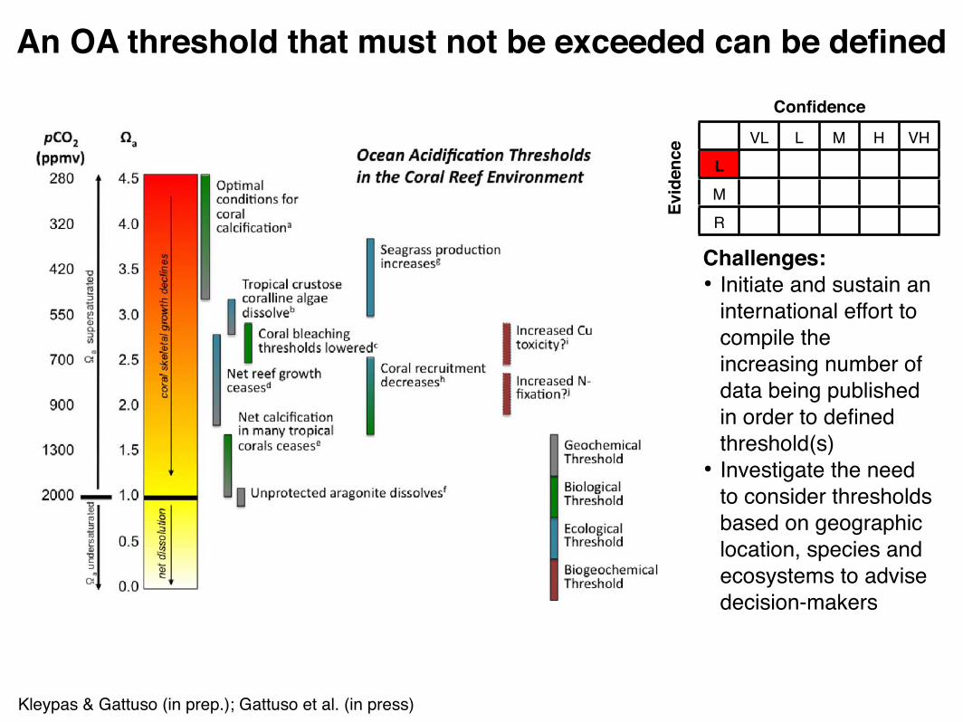
An OA threshold that must not be exceeded can be defined
VL L M H VH
L
M
R
Confidence
Evid
ence
Kleypas & Gattuso (in prep.); Gattuso et al. (in press)
Challenges:• Initiate and sustain an
international effort to compile the increasing number of data being published in order to defined threshold(s)
• Investigate the need to consider thresholds based on geographic location, species and ecosystems to advise decision-makers

Summary on statements
• Chemical effects: robust evidence and high certainty
• Biological and ecological effects: much less certain• calcification, primary production, nitrogen
fixation and biodiversity will be altered but with an unknown magnitude
• some cannot be assessed• Biogeochemistry, society and the economy
may change; whether it will be significant or not is also unknown

Systems at risk
• Polar areas• Deep-sea environments• Coral reefs• Nearshore ecosystems

Past limitations and future prospects
• Limited workforce and funding• Inappropriate or inconsistent methods• Duration of experiments• Interactions with other stressors• Lack of field evidence other than around CO2 vents• Limited work at the community level• Difficulties to perform meta-analysis• Model development• Need for a coordinated international effort
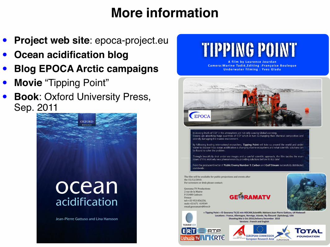
More information
• Project web site: epoca-project.eu• Ocean acidification blog• Blog EPOCA Arctic campaigns • Movie “Tipping Point”• Book: Oxford University Press,
Sep. 2011
TIPPING POINT
!
!
! !
!
! " # $ %& " '( " ) *+ ,-. /- " 0 1+ ,2*.3*&-,* 45* , $ .- " 6*2 $ 7 8 92 $ : $ . ; " 4 < ,*. =1 $ > - " ?1+ % -@+-
A.2- ,B*:- , " # $ %& $ .; " 4 " CD- > "E % *2+
!"#$%%$&'"()$&*"+","-.)/010"#2345"1$&"6789:3;<$.&=><"9?@$A./ABC.0&"($.//."-0DEA)3"FGH"I$.J.A.GGK)<0=)&A"B"L/0&<.3"9GG.10'&.3"M)/@N'.3"OAG0&?.3"MPQRG.AE&?""S;%$*TJ./'U3"F;9"
;V))=&'B:0$"W"X<*"5YZY37.G$@./P"7.<.1J./""5YZY2./A$)&A"B"L/.&<V"0&?"[&'G$AV
!"#$%&'($)&''$*#$+,+&'+*'#$-./$01*'&2$0/.3#24&.56$+57$#,#546$+-4#/$4"#$89:8;:;<8<=$>./$62/##5#/6$./$7,76$0'#+6#$2.54+24?
@#./+(+$!A$B/.7124&.56;$/1#$7#$'+$C+&/&#>DE8FG<$H+7.1/6>/#52#4#'IJEE$K9E$G9L;9<M(.*?JEE$LN8$$F8K9FK#(+&'?O#./+(+4,P-/##=-/
12/11/10 16:52Welcome to the EPOCA web site!
Page 1 sur 2http://www.epoca-project.eu/
Search ...
Menu
HomeWho are we?What do wedo?DataGuide to OAresearchWhat is oceanacidification?Dissemination& media centerRestricted areaContactNewsSitemapLinks
Login
Welcome to the EPOCA web site!
French Italian German Dutch Russian
The EUFP7IntegratedProjectEPOCA(EuropeanProject onOCean
Acidification) was launched in June 2008 for 4 years.The overall goal is to advance our understanding ofthe biological, ecological, biogeochemical, andsocietal implications of ocean acidification.
EPOCA aims to:
document the changes in ocean chemistry andbiogeography across space and timedetermine the sensitivity of marine organisms,communities and ecosystems to ocean acidificationintegrate results on the impact of oceanacidification on marine ecosystems inbiogeochemical, sediment, and coupled ocean-climate models to better understand and predictthe responses of the Earth system to oceanacidificationassess uncertainties, risks and thresholds ("tippingpoints") related to ocean acidification at scalesranging from sub-cellular to ecosystem and localto global
The EPOCA consortium brings together more than 100researchers from 29 institutes and 10 Europeancountries (Belgium, France, Germany, Iceland, Italy,The Netherlands, Norway, Sweden, Switzerland, UnitedKingdom).
EPOCA is endorsed by:
EPOCA summary in different languages:
Ocean acidification blog
The EPOCA blogprovides dailyupdates onscientific articlesand mediacoverage onoceanacidification
News
Erratum to the“Guide to BestPractices forOceanAcidificationResearch andDataReporting”Oceanacidification -questionsansweredOceanacidificationand its impacton polarecosystemsLe Muséeocéanographiquede Monacoaccueille “The2010 AnnualOceanAcidificationReference UserGroup Meeting”EPOCA andCarboSchoolshands-onexperiments onoceanacidificationErratum to the"Guide to BestPractices forOceanAcidificationResearch andDataReporting"INVITATION:EPOCA,BIOACID andUKOARPstudentsmeeting 2010
ocean acidificationJean-Pierre Gattuso and Lina Hansson
B IOLOGY

Thank you for your attention!• Lina Hansson, EPOCA Project Manager
• book authors, especially co-authors of final chapter:• Jelle Bijma• Marion Gehlen• Ulf Riebesell• Carol Turley
• Anne-Marin Nisumaa, EPOCA Data Manager
• EPOCA consortium
• Funding from the European Commission
Acknowledgements
ocean acidificationJean-Pierre Gattuso and Lina Hansson
B IOLOGY