ACI JOURNAL TECHNICAL PAPER Title no. 81-29

Bayesian Statistical Prediction of Concrete Creep and Shrinkage

by Zden~k P. Batant and Jenn-Chuan Chern

In present design practice, the statistical approach is used for strength but not for deformations, including creep and shrinkage. However, predicting concrete creep properties from design strength and con­crete composition involves a large uncertainty, much larger than that of strength. It is shown that by carrying out some short-time creep measurements, even rather limited ones, the uncertainty can be drastically reduced, and extrapolation of short·time measurements can be made much more reliable. This is accomplished by developing a Bayesian approach to creep prediction. Prior information consists of the coefficient of variation of deviations from the creep law for concrete in general, as determined in a recent statistical analysis of the numerous creep data that exist in literature. This information is com­bined, according to Bayes' theorem, with the probability of a given concrete's creep values to yield the posterior probability distribution of the creep values for any load duration and age at loading.

Only a linear creep case is considered, and a normal distribution of errors is assumed for the given concrete as well as for the prior infor­mation. To demonstrate and verify the method developed, various creep data reported in literature are considered. Predictions made on the basis of only a part of the test data are compared with the rest of the data, and very good agreement is found. The effects of various amounts of measured data, and of various degrees of uncertainty in the prior information, are also illustrated. The present approach is recommended for concrete structures for which the creep deflections, creep-induced cracking, or creep buckling are of special concern, e.g., nuclear reactor vessels and containments, certain very large bridges, shells, or building frames.

Keywords: Bayes theorem; concretes; confidence limits; creep properties; er­rors; probability theory; regression analysis; shrinkage; statistical analysis; structural analysis; structural design.

Creep and shrinkage appear to be the most uncertain phenomena with which a designer of concrete struc­tures must cope. The statistical variability of creep and shrinkage is much larger than that of concrete strength, yet so far statistical methods have been well developed only for the latter. This is partly because the problem is more difficult and partly because the consequences of a substantial error in predicting creep and shrinkage are generally less disastrous than they are for strength. Ex­cept for creep buckling, errors in creep prediction and shrinkage do not cause structural collapse but merely put the structure out of service due to excessive deflec-

ACI JOURNAL I Julv-Auaust 1984

tions or excessive cracking (which causes reinforcement corrosion). Nevertheless, for reasons of economy, it is very important to improve the prediction of the effect of creep and shrinkage in structures and, in particular, design structures for certain extreme rather than aver­age creep predictions.

Probabilistic analysis of concrete creep and shrink­age has recently been rendered possible by extracting extensive statistical information from literature (see Reference 12, in which data for 80 different concretes, consisting of over 800 experimental curves and over 10,000 data points, have been analyzed statistically and organized in a computerized data bank). It appears that if no measurements for a given concrete to be used are made, the uncertaint~ in predicting its creep and shrinkage on the basis of the chosen concrete mix pa­rameters and chosen design strength is enormous. Even with the most sophisticated and comprehensive predic­tion model,12,13 prediction errors (confidence limits) ex­ceeded with a 10 percent probability are about ± 31 percent of the mean prediction. 1J For the 1971 ACI Committee 209 Model, I which is much simpler, this in­creases to about ± 63 percent, and for the 1978 CEO­FIP Model Codel6 to about ± 76 percent. This is clearly an unsatisfactory state of affairs.

It has been demonstrated, however, that drastic im­provement is possible if some experimental data, even very limited short-time data, are obtained for the par­ticular concrete to be used. 12

,13 For a creep-sensitive structure, such as a nuclear reactor vessel, large shell, or large bridge, the designer usually has at his disposal some limited short-time test data for his concrete. Con­sidered by themselves, extrapolation of these data to long times would also be very uncertain (for an exam-

Received Apr. 28, 1983, and reviewed under Institute publication policies, Copyright © 1984, American Concrete Institute. All rights reserved, including the making of copies unless permission is obtained from the copyright propri­etors. Pertinent discussion will be published in the May-June 1985 ACI JOUR­NAL if received by Feb. I, 1985,

319

Zdenek P. Bazant, FACI, is a professor and director, Center for Concrete and Geomaterials, Northwestern University. Dr. Bazant is a registered structural engineer, serves as consultant to Argonne National Laboratory and several other firms, and is on editorial boards of five journals. He serves as chairman of RILEM Committee TC69 on creep, ASCE-EMD Committee on Properties of Materials, and IA-SMiRT Division H. His works on concrete and geomater­ials, inelastic behavior, fracture, and stability have been recognized by a RILEM medal, ASCE Huber Prize and T. Y. Lin Award, IR-JOO Award, Guggenheim Fellowship, Ford Foundation Fellowship, and election as Fellow of American Academy of Mechanics.

Jenn-Chuan Chern is a scientist at Argonne National Laboratory. In June 1984 he received his PhD in civil engineering from Northwestern University. Prior to coming to the U.S., he worked for two years as an engineering lieutenant in the Chinese Marine Corps and for one year as a structural engineer on the design and construction of petrochemical plants. His research interests include con­crete creep, moisture effects, cracking, and high temperature effects on con­cretes, on which he co-wrote a state-of-the-art report for the Electric Power Research Institute. He has also developed a large computer code now in use in some government laboratories.

pIe from a nuclear containment design, see Reference 8). A great improvement is, however, possible if the statistical information for the given concrete is com­bined with prior statistical information for all similar concretes, such as that presented in Reference 12 or 13. This is the subject of Bayesian statistical analy­SiS.4,14,22,25,27,29-3I,36,37,40 Application of this concept to the present problem is the objective of this work.

From the physical viewpoint, the causes of random­ness in concrete creep and shrinkage are basically threefold: (1) randomness due to uncontrollable varia­tions in material properties; (2) randomness due to variations in the environment (weather); and (3) ran­domness of the creep increments due to the statistical nature of the creep mechanism itself. 18 The first of these three causes of uncertainty is by far the worst and may be largely eliminated by carrying out a few limited measurements and applying the Bayesian analysis that follows. The second and third causes then remain, and the worse one of these is randomness of environment. A separate study, based on spectral analysis of stochas­tic processes, has recently been devoted to this aspect. By environmental control in the laboratory, or due to mass concrete conditions, the second cause is largely eliminated, and if the properties of the given concrete are determined well by measurements, randomness of the creep mechanism then remains as the principal re­maining cause of uncertainty. For the sake of simplic­ity, the study does not attempt to distinguish between the aforementioned different physical causes, but we should at least be aware that the purpose of Bayesian analysis is to eliminate the first of the three causes. Measurement errors from the creep predictions are also not eliminated.

The problem at hand exhibits various mathe­matical similarities with some other Bayesian problems.4,14,25,27,30,3I,35-38 This is true of Tang's35 Bayesian analysis of future settlements of an oil platform for which some short-time settlements have been observed.

In this study, we aim only at determining the creep and shrinkage properties of a given concrete. Use of these properties in structural analysis is another prob­lem that cannot be included in this study.

320

The error of measurement should be eliminated from test data used in the present analysis, since this error is not felt by the structures. If many readings at closely spaced time intervals are taken, it may be assumed that this error is approximately eliminated by hand-smooth­ing of the measured curves.

Linearization of creep law and its error As a reasonable approximation for many practical

situations, the creep law of concrete may be considered to be linear, i.e., obeying the principle of superposi­tion. Creep is then fully characterized by the compli­ance function J(t, I') (also called the creep function), which represents the strain (creep plus elastic strain) at age I caused by a unit constant uniaxial stress acting since concrete age I' .6 For the purpose of statistical analysis, it is helpful to express the compliance func­tion in linearized form

(1)

in which ~ is a certain reduced time and 01, O2 are ma­terial parameters. Various creep prediction formulas can be brought to the form of Eq. (1). We choose here the double power law6,7,ll-13 because it was shown to agree better with test data than other well-known for­mulas. For this law

cPI 01

= -, O2

= -, Eo Eo

~ (I, I') = (I' -m + a) (t - t')" (2)

in which Eo, cPl' m, n, and a are material constants. Their typical values are m = 0.3, n = V8, a = 0.05, and cPI = 2 to 6; however, the scatter is consid"''''' hle." Empirical formulas for estimating these par '<;

from concrete strength and composition exist. 12,. able ~ may be called the reduced time; 01 is a creep L

parameter, O2 is the instantaneous deformation (for in­finitely rapid loading), and Eo is called the asymptotic modulus, typically Eo ::: Ee where Ee is the conven­tional elastic (static) modulus, which corresponds to a load of about two hour duration and involves much short-time creep. Note that the earlier use of Ee instead of Eo in the power law for concrete creep does not per­mit an adequate representation of longtime creep be­cause it results in a much too high value of n.6

All the material parameters in the creep law, i.e., Eo, cPI' m, n, and a are, strictly speaking, random var­iables. However, to make our problem tractable, only those parameters that appear linearly in J(t,t') can be considered random. According to the linearization in Eq. (1), these are the parameters 01 and O2, whose vari­ations represent a vertical shift of the creep curves and a change in their overall slope. Although, in principle, it would be more realistic to apply factor analysis to re­duce the number of random material parameters, we cannot do so since independent statistical data for these parameters are unavailable. Statistical information ex-

ACI JOURNAL I July-August 1984

ists only for the compliance values, which leads us to the following statistical model

J(I, I') = Ol~ + O2 + e (3)

where e is the error. We will consider that e has a nor­mal distribution with mean 0 and standard deviation (J.

Although the creep compliance depends separately on the current time I and the age at loading I' , these two variables are grouped under one independent variable ~. This is one essential idea of the present analysis, which permits us use of prior information on creep at any I and I'.

Bayesian estimation We consider J as a random variable for which the

governing law [Eq. (1) and (2)] is known with a high degree of certainty, but the material parameters 01, O2

are rather uncertain. Assume that the probability den­sity distribution f' (01, ( 2) of the possible values of 01

and O2 is known from prior testing of various con­cretes. This distribution is called prior. The probability that OJ (i = 1, 2) lies within the intervals (01, 01 + dOj) may be denoted as P(01 < OJ < 01 + dO;) and equals l' (01, (2)dOI d02.

Now suppose that, for a given concrete of interest, certain compliance values"" at reduced times ~j (j = 1, 2,. . ., N) have been measured. We want to exploit this information to obtain an improved (updated) probabil­ity density distribution f"(OI' ( 2) of parameters 01, O2, given that compliances JI(~I)' ... , JJ..~N) have been measured. This distribution is called posterior. The conditional probability that OJ lies within the intervals (01, 01 + dOj), given that Ji~) has been measured, may be denoted as P(Oj* < OJ < OJ* + dOjIJI, . .. , I N) and equals f"(OI' (2)dO ld02. According to Bayes' theorem 4,S,I4,I S ,22,27 ,30,39,40

P (OJ* < OJ < 01 + dOMj, . , ., I N) = kP (JI, ... , JNIOj) P (01 < OJ < 01 + dO;) (4)

where k is a normalizing constant assuring that the sum (integral) of all probabilities P(Oj* < OJ < OJ* + dO;jJI,. .. , I N) is unity, and P(JI, . .. , JNIOj) is the probability of measuring values ""(~) under the condi­tion that the parameter values are OJ' Introducing the foregoing expressions for P( . .. ) in terms of f' (01, ( 2)

and f'(OI' ( 2) and dividing by dOld02, we obtain from Eq. (4)

in which L(OI' O2; JJ) = P(JI, . , ., JNIO;). This func­tion is called the sample likelihood function, The nor­malizing constant k is determined from the condition

"" "" J J 1"(01, ( 2) dOl d02 = 1 (6)

Supposing, for the sake of simplification, that the observed values J I , J2 , ' •• , I N are statistically inde-

ACI JOURNAL I July-August 1984

pendent, we may express the sample likelihood func­tion as

N

II jj (",,101, ( 2) J "" I

(7)

Here, jj(Jj l0\>02) is the probability density distribution of one random variable "", given that parameter values are 01 and O2, i.e., jj(Jj IOI,02)dOld02d"" is the probability that the Jrvalue lies within the interval ("", Jj + dJ) under the condition that the parameter values lie within the intervals (OJ, OJ + dO;). For one particular concrete, pa­rameters 01, O2 are fixed, and so jj(""IOI,02) describes the scatter of Jrvalues in one and the same concrete.

According to our statistical model [Eq. (3)], the compliance"" for certain parameter values 01, O2 and a certain fixed reduced time ~j is a normal random vari­able with the mean (Ol~j + (2) and standard deviation (J, i.e.

Standard deviation (J is to be evaluated for fixed 01 and O2, i.-e., fixed material properties. Thus, (J characterizes the scatter of J for the given concrete for which mea­surements "" were taken, If these measurements do not suffice to determine (J for this concrete, a typical value of (J for any similar concrete may be used for which plentiful data exist.

Assuming (J to be independent of reduced time ~ and substituting Eq. (8) into Eq. (7) and Eq. (7) into Eq, (5), we obtain the result

The normalizing constant k follows from Eq. (6)

The posterior (updated) expectation of parameter OJ, given that the observed compliance values were Jj , may be obtained as

"" "" J J OJ"(OI' (2) dOl d02 (11)

where E denotes the expectation. The posterior (up­dated) probability that the compliance J(~) at reduced

321

time ~ will be less than some given value J may be cal­culated as

P [J(~) < J]

J J P [J(O < J\O" O2] 1"(0" (2) dO, d02 ~ ~

J J <I> [y (0" ( 2)] = 1"(0" ( 2) dO, d02 (12)

where <I> represents the cumulative normal distribution function

<I> (y) = ~ J 2

e -x 12 dx (13)

and

(14)

It is convenient to use a prior distribution that yields a posterior distribution of the same type; this is called a conjugate prior. 4 For a normal distribution, the con­jugate one is again a normal distribution.4 Therefore, for l' (0,,02) the normal distribution is chosen. Because two parameters are used, a bivariate prior distribution should be properly considered

where m" m2 are the means and <J" <J2 the standard de­viations of 0" O2 , Unfortunately, however, no statistical data have yet been published for the parameters 0, and O2,

To circumvent this difficulty, we may consider the univariate distribution of the values of J(O and assume it to be normal

z (0)

f [J(O] 1 ll(l(0-J(O)2l (16) .J27r <JAO exp -2: <JAO

Here, l(~) = mean of the (prior) observations of J at reduced time ~, and <JA~) = their standard deviation, which may be calculated as <JAO = wJl(n where WJ =

coefficient of variation of the prior data, which is con­sidered, for the sake of simplicity, to be independent of reduced time ~. Extensive data on the values of W J are given in Table III of Reference 12 and in Table 2 of Reference 13.

Now, we come to an important step; if we substitute J(O = O,~ + O2 , this distribution becomes a function of (), and ()2' Furthermore, noting that I1J = ~ 110, + 11()2' we see that the probability (or frequency) of error I1J =

~ 110, at 11()2 = 0 is the same as the probability (or fre­quency) of error 110" and the probability of error I1J =

11()2 at 11(), = 0 is the same as the probability of error 11()2' Therefore, on substitution of J(O = (),~ + ()2' Eq. (16) may be regarded as an approximate probability density distribution of (), and ()2' i.e.

Replacement of the bivariate distribution [Eq. (15)] with a univariate distribution [Eq. (17)] is a crucial step in the present analysis, allowing the use of existing sta­tistics of creep data. A similar step was used by Tang et al. 37 in their analysis of settlement of oil platforms.

Numerical integration Integrals of the type of Eq. (12) must be evaluated

numerically. Caution is required, since the integral ex­tends over an infinite domain. From the practical view­point, this is usually the most sensitive task in Bayesian analysis, and various studies have been devoted to iL'7,26 None of them, however, seems to be directly applicable to the present integrand.

Fig. l(a) shows the shape of the exponents of the functionj"(0"()2) for the case whenf'«(),,02) = 1 (dif-

(b)

v u

--------~--~--~------ 9,

Fig. 1-(a) Exponent of function 1" (()" (}2); (b) transformation of coordinate sys­tem

322 ACI JOURNAL I July-August 1984

fuse prior); the integration was done with 40 integra­tion points for both 01 and O2 , and the statistical param­eters of the test data by Rostasy33 were considered. The surface decays rapidly in one direction and extremely slowly in another. For this reason, it is necessary to in­troduce new independent variables u and v, which con­vert the bivariate normal distribution to a standard form.

Function f'(OI,02) that needs to be integrated in the integrand of Eq. (12) may be written, according to Eq. (9), in the form

f"(OI' ( 2) = ao exp [ - (AO~ + BOT + 2DOI02 + 2E02 + 2FOI + G)] l' (01, (2) (18)

with coefficients

N 1 A=-+-- B

20-2 20-2,,(0 '

N _ _ ~_2_ E ~J +

20-2 j = I 2U.,(~)2 ' 1 N ' ~

D--~t+--- 20-2 j~ <;,j 2U"(02 '

1 N :r (~) E = - 20-2 j~ Jj - 2U"(02 '

1 N ~:r(O F = - ~ tJ --

- 20-2 j~ <;'i i - 2U.,(~)2 '

G = _1_ t J2 + :r(~)2 20-2 j = I J 2U"(02

(19)

where N = number of observed creep data. In the spe­cial case of a diffuse prior [I' (0 1, ( 2) = const.], the second terms in these expressions vanish because U.,(~) --+ 00. We seek to transform Eq. (18) to the form

where u, v are new variables given by a certain linear transformation [Fig. l(b)]

u = a02 + bO I + c, V = (a02 - b()1 + d) -Ii (21)

which transforms the quadratic polynomial in Eq. (18) to its principal coordinates. Comparison of the coeffi­cients in Eq. (19) and in Eq. (20) and (21) yields the re­lations

(22a, b)

ab(1 - e) D, ac - ebd E, (22c, d)

be + ead F, cZ+e~ G (22e, f)

Further, one needs to solve from these equations a, b, e, d, e under the conditions that a, b, c, d, e are real and a > 0, b > 0, and e > 0. After some tedious al­gebraic manipulations, one can show that such a solu­tion exists, and one solution (with e < 1) is

ACIJOURNAL I July-August 19PA

a (A - eB)Y', b = (B - eA)Y', 1 - e 1 - e

aE + bF aF - bE ---, d= ' a2 + b2 e(a2 + b2)

e

A + B - [(A - B)2 + 4V]Y2

A + B + [(A - B)2 + 4V]y' (23) e

which can be verified by substitution into Eq. (22a-f). Another solution exists (with e > 1), but it is equiva­lent since it merely corresponds to interchanging u and v. The inverse of the linear transformation in Eq. (21) is

[a(e-Y'v - d) + b(u - e)](a2 + b2)-1 [a(u - e) - b(e-Y'v - d)](a2 + b2)-1 (24)

and the Jacobian of the transformation in Eq. (21) is

In the integrals in Eq. (11) and (12), we may now sub­stitute

in which Eq. (24) must be substituted for 01 and 02' The integration over u and v is to be carried out from - 00

to 00.

The integrals may be efficiently evaluated using the Hermite-Gaussian formula which has, for the variable,

2 the form I~ .. I(x)e- x dx = En wJ(x,J, where Wn is cer-tain known weights. 34 In the case of two variables [Eq. (26)], this integration formula yields for the integral in Eq. (12) the approximation

1 K M

P[J(O < J] = - E E WkWm ~(Ykm) (27) '7rk=lm=1

in which K and M are the chosen numbers of integra­tion points for coordinates u and v, and ~(Ykm) is given by Eq. (13)

and Olkm' 02km are evaluated from Eq. (24) for u = Uk and v = vm•

Eq. (27) is the final result to be used in computer calculations.

Examples To demonstrate the theory, consider the test data by

McDonald.28 From the fitting of these data, one obtains double-power law parameters m = 0.305, n = 0.147,

323

and ex = 0.059,12 and based on the scatter of these data (fixed 01, ( 2), it can be roughly estimated that (J ""

0.01 X 1O-6/psi. The prior information may be deter­mined from the BP modeP2 using the following param­eters: cylinders 15.2 x 40.6 cm, sealed, at 23 C, 28 day cylindrical strength 6300 psi, water-cement-sand-gravel ratio 0.425 : 1 : 2.03 : 2.62, cement type II, and age at loading t' = 90 days. Furthermore, the value of coef­ficient of variation for all concretes (prior information) may be considered as W J = 0.24, according to Refer­ence 12 (provided the BP model is used).

To get an idea of the usefulness of the Bayesian ap­proach to creep prediction, the prediction for varying amounts of data for the given concrete (i.e., for pro­gressively better likelihood functions) is given in Fig. 2. First Fig. 2 shows the predicted 90 percent probability band and the mean for the concrete of McDonald if the prediction was based strictly on the prior information, i.e., if the data of McDonald were not known to us. Furthermore, Fig. 2 also shows the Bayesian prediction of the mean creep and the 90 percent probability band when only the first four data points of McDonald are known, and also when the first eight points are known.

It should be noted that the 90 percent probability band progressively narrows with the increasing amount of data for the concrete of McDonald and that the me­dian prediction comes closer to the remaining later data not used in the prediction. The most significant im­provement of prediction is brought about by consider­ing the first data point [Fig. 3(a)].

Also note that the width of the 90 percent probabil­ity band (scatter band) increases with increasing time. This effect is particularly pronounced when assuming constant W J ; if (JJ were assumed constant, the width of

04

-; ~ T 0.3 o .-4

-~ ~0.2 ..,

0.1

McDonald 1975.lIeale~ / t'=90days / (1 = 0.01 x 10-6/ps i /

with prior //N=4

/'

/' ./

/'

....- -"'"'... prior 90"0

....-....-./ N ~8

./ ............ ...... --- 0 0 Data used in analysis

x x Data not used

10 1 102

t-t' (days)

Fig. 2-Prior, posterior median and probability band UJ90for McDonald's test data

~?4

the probability band would not increase so markedly with time.

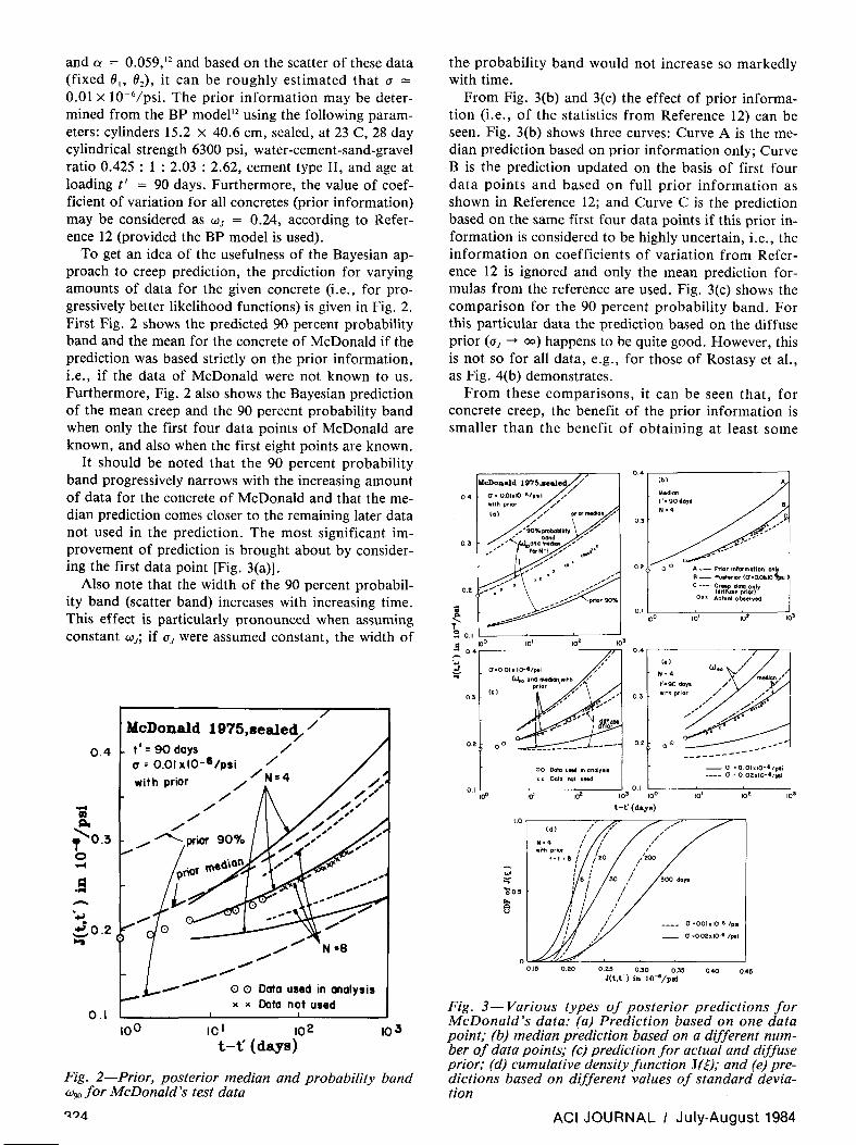
From Fig. 3(b) and 3(c) the effect of prior informa­tion (i.e., of the statistics from Reference 12) can be seen. Fig. 3(b) shows three curves: Curve A is the me­dian prediction based on prior information only; Curve B is the prediction updated on the basis of first four data points and based on full prior information as shown in Reference 12; and Curve C is the prediction based on the same first four data points if this prior in­formation is considered to be highly uncertain, i.e., the information on coefficients of variation from Refer­ence 12 is ignored and only the mean prediction for­mulas from the reference are used. Fig. 3(c) shows the comparison for the 90 percent probability band. For this particular data the prediction based on the diffuse prior «(JJ --> 00) happens to be quite good. However, this is not so for all data, e.g., for those of Rostasy et al., as Fig. 4(b) demonstrates.

From these comparisons, it can be seen that, for concrete creep, the benefit of the prior information is smaller than the benefit of obtaining at least some

04 u- O.OhllO-e/pll

0.3

0.2

11

~ ~ 0.1 L--__ ~_~~_----' .s CO 10' 10

2

~ 0.4;=---"--------7/1

~ cr-O.QllIlo-6/pei "

w'o and rntIdic.l,with ;'

(0) 0.3

0.2 00

prior

00 Data uMd in analYIls •• Data not uNd

---_ a -O.OI1l1O-6/pl i ____ cr "O.02xIO-I'pll

0.' '-;'rf'o------'oIO'---''::;o'----:"lo3 0.1 L,OO,----,~Ol---,'-::O.---"o.

t-t· (da,y.)

0.20 0.2' 0.30 O.M 0.40 O.4~ J(t.t') in lO-"/p.i

Fig. 3- Various types of posterior predictions for McDonald's data: (a) Prediction based on one data point; (b) median prediction based on a different num­ber of data points; (c) prediction for actual and diffuse prior; (d) cumulative density function J(~); and (e) pre­dictions based on different values of standard devia­tion

ACI JOURNAL I July-August 1984

0.5 r------------r-------,,,.......,...., 0.5 ~

to} // \bl JIo-.".ToIch ... ,ZDcelll: •• 187} .-

RH >95% ,,/ t l .28daYI .,,/ 11

l>o

"04

'" .... .!l .... .; O.~ 0:;-

0.2 ......... -----'-,,.------'-7""""""=-----~----' 0.2 '0 ' 102 10'

t-t·(dll.Ylll 10 10" 10'

0.5 10 , , , , , /

, , , \d I , , (e I / / O=O.OIXlo-tvr-{

, , , / .~

, , :' II o ·0.01 x IO~1 /psi , , with prior I

~ ~ I ,,/ with prior , / ___ N-4 I T 0.4 , / tJ _ N-I. ,

'" .... , , Prior me<lkm 0:;-, - : ,

.s -,- "0 O.~ /'00 -- I ...........

~ t- ,'.7 f .... ,/ ~ 0.3

u I ... I / , /1 ,

:' , / " 02

0.28 0.36 0." J(t.t') in lO-O/pll

Fig. 4-Various types of posterior prediction for Rostasy et al. 's data: (a) Predic­tion based on prior and different numbers of data points; (b) same as (a) but for diffuse prior; (c) prediction based on first data point only; and (d) cumulative den­sity function J m

O.B 0.8

Shuta Dam 1953.1958.sealed (bl

t'·28day • (a) 0- 0.01 .,o-l/pOl .... N-2 .. (J" 0.01.'0-8/P1 i -e: _ Act.al prior T 0.6 with prior 0.6 --- Shifted prior 0

priar 90~~ .. oS J.......... ",-

" --. ...-- -" ~ 0.4

---- ........ 00::::.',-·-' 0 .• o _'-'-;'"

'i::;' -- N-.

__ ...-,,-..-~ prior median .-'" ,-,----0.2 -- 0.2

100 10 ' 10' 103 10° 10 ' 10' 10 3

t-t'(da,ys)

Fig. 5-Various types of posterior predictions for Shasta Dam concrete: (a) Pre­dictions based on actual prior and various numbers of data points; and (b) effect of shifting the prior upwards

short-time creep data for the given concrete. (A similar conclusion was reached empirically in Reference 13.) This last conclusion is further reinforced by the predic­tion in Fig. 3(a), which is based on the full prior but only the first data point of McDonald and on the knowledge that a is roughly 0.01 x 10 - 6/psi for these data. The mean prediction agrees surprisingly well with the rest of the data of McDonald. (This case is called a "dominant prior" and a "soft Bayesian prediction. "27)

From Fig. 3(d) an idea of the shape of the cumula­tive probability density function <I> (y) can be drawn for the J(n values at various t - t I, obtained for Mc­Donald's data, according to Eq. (12) or (27).

To show that similar results are obtained for other creep data from literature, predictions have been cal-

ACI JOURNAL / July-August 1984

culated for the test data of Rostasy et alY and for Shasta Dam data23

,24; see Fig. 4(a) through (d) and 5(a) and (b). There are some differences, however. For the data of Rostasy et aI., the measured points happen to lie closer to the median of the prior, much more so than for other test series. Nevertheless, use of the prior still does improve the prediction based on a reduced num­ber of data points (N = 4, N = 8, and N = 14). For Shasta Dam concrete, the opposite is the case; the mea­sured data lie far off the prior median prediction, and this is why the posterior curves are so different. Espe­cially note that the first two data points combined with the prior give a very poor extrapolation to longer times, much poorer than that for the concrete of Rostasy et al. and of McDonald.

325

o.5,..-----------------"A 0.5.---------------..,."

0.4

0.3

(0) Rostaay,Teichen,Engelke,1971

,t -28days N-44 OR- 0.05 1l IO-6/ps i

02 L-~_~_~_~_~_~_~~

0.4

(b)

N-44

o,,_O,oexIO- 6 /psi

10'

J(t,t') - (0.34C +0.081l> 10-1

10 0.4 0.6 0.8 \.0 \.2

~ 0.5,..----------------""']0.5 r-(-d)--------------,

(c)

.; -e: 0.4 T = ... . S

~ 0.3 ';:;'

N - 4 O •• O,OlxIO-6/pli

--------J (t, t')-(0233t +0.134)010-'

04

0.3 ra9r ... ion mad ian

J(I,t')-(0.233f. + 0.134) 010..8

0.2 L..,-----L-:----~=__--'"":-------' 0.20L...4-~-0.,...6-~--t~.8-~-..J..1.0:--~--'I. 2 10° 10' t-/(':"ys) 103 10·

0.5 r-(.-) --------------,0.5.--------------------, (f)

N -8

0.4 O'A-O,02x 10 .. 1 IPI'I

0.4

0.3 0.3

J(t, t') -(0.273t+0119)xI0

N-8

0'.-0.02010-6/PIi

/~

",,'" rIQre •• ion median , " ~, J(t,t')-(0.273t +0.1I9hlO-1

0.2 '--~-~-~-~-~-~-~--'0.2 L-__ ~_:_--~=__--~----' 0.4 0.6 0.8 1.0 1.2 100 10' 102 103 10'

t t-t'(days)

Fig. 6-Regression analysis of Rostasy et al. 's data for various numbers of points. (a), (c), and (e) in linear plots and (b), (d), and (f) same as in log (t - t') plot

The prior information greatly modifies the predic­tion when the measured data lie outside the 50 percent probability band Wso of the prior. An example of this is artificially constructed in Fig. 5(b), in which the actual prior median was deliberately shifted upward, keeping the data as measured. We see that such a shift has a great effect on the median and makes the posterior probability band wider.

It is interesting to contrast the Bayesian analysis with simple statistical regression based on only measured data and prior knowledge of the formulas for the mean values; see Fig. 6(a), (c), and (e) showing the linear regressions made in the ~ scale as well as corresponding plots in log(t - t') scale in Fig. 6(b), (d), and (f). If only a few data points, e.g., four points in Fig. 6(c) are used, the probability band rapidly widens with time, while for a long data series [Fig. 6(a)] it remains nar­row. In the latter case, the probability band might be narrower than that obtained from Bayesian analysis with all the prior information, but the Bayesian ap­proach is more realistic.

326

It should be noted that, while extrapolating data of statistical regression, one is predicting statistical prop­erties of the future creep of the particular specimen measured. On the other hand, in our Bayesian analysis, we are predicting statistical properties of creep of all the specimens that could possibly be made from the given concrete. It is the latter case which is of interest for de­sign, and the statistical' variability for this case is ob­viously larger.

Determining standard deviation (J for the likelihood function is important. (J characterizes the scatter of J­values at some fixed time when a great number of iden­tical creep tests on a given concrete (fixed 01,(2) is per­formed under the same conditions. Such data have re­cently been presented by Cornelissen, Reinhardt et al., and Alou and Wittmann.3.19.20,32 One typical example from the Reinhardt et al.'s results is shown in Fig. 7, from which one can see that for their concrete roughly the value (J = 0.02 x 1O-6/psi would be appropriate for characterizing the likelihood function for the sum of creep and shrinkage strains. Strictly speaking, (J de-

ACI JOURNAL I July-August 1984

0.8 r--------------------,

... 0.6 I o .... >< '-'

0.2

Reinhardt et al .• 19BO

Mix 3

Number of splcimen, -8

x Mldian

I WIO _C1

o~~==~~==~~~==~====~ 10 50 100

t-t' (days)

Fig. 7-Reinhardt et al. 's statistical data for identical specimens

pends on time, as can be seen from Fig. 7, although it was neglected in the foregoing analysis. To avoid the need for many tests for the given concrete, it may also be assumed that a is the same as observed before on similar concretes. Note that the a-value for the likeli­hood function is different from the value of standard deviation that results from a regression analysis of one creep test (with many i-values for different times but the same specimen, as shown in Fig. 6).

The effect of various choices of a (for the likelihood function) is shown in Fig. 3(e). A smaller a, if justified, gives a distinctly better median prediction and a nar­rower probability band.

As can be seen from these examples, the value of standard deviation a for the concrete under considera­tion has a great influence on the width of the scatter band for creep extrapolation. At the same time, the di­rect information on a is usually scant, since only few measurements are normally carried out for the concrete at hand. In such situations, the value of a has to be based on an analysis of the data for various similar concretes. For these predictions, the standard devia­tions for the data of Rostasy et al. and Shasta Dam data were estimated as w = 0.01 x 1O- 6/psi. For the prior predictions according to Reference 12, the fol­lowing information was needed: Shasta Dam data -Cylinders 15.2 x 66 cm, 21 C, sealed, 28 day cylinder strength 3230 psi, water-cement-sand-gravel ratio 0.58 : 1 : 2.5 : 7.1, cement type IV, m = 0.376, n = 0.127, a = 0.043, and t' = 28 days. Rostasy et al. data - Cyl­inders 20 cm diameter and 140 cm length, environmen­tal relative humidity ~ 95 percent, temperature 20 C, 28 day cube strength 6500 psi, water-cement-sand­gravel ratio 0.41 : 1 : 2.43 : 3.15 (by weight), and age at loading t I = 28 days.

One notable simplification in our statistical model is that the values ii, i 2, . .. , iN' as well as similar data for the prior, are implied to be statistically independent, but in reality they are not completely so. If, for exam-

ACI JOURNAL I July·August 1984

0.8r-----------------------------------,

." III ~ ,0.6 T o ....

-+> ..; 0.4. -.,

Shasta Dam I953.I95B.sealed

C1=0.01 10_8/psi

with prior

t' ·28 days

•• 0.0

W90

and median for .x

N"8 •

•• In •• rtM data for anal,.l.

00 Oa'a n.d In analy.i •

• • Data not uud 0.2~ ________ L_ ________ L-________ ~ __ ~

10 1 102

t-t'(days)

Fig. 8-Effect of spacing of data points on the predic­tions

pIe, the creep value is high, compared to the mean, at ~ = 1000, it will be high at ~ = 1001 and will be quite close to the value at ~ = 1000. This is so because, in the physical mechanism of creep, the randomness arises through creep increments rather than their accumu­lated values. IS The correlation of adjacent i-values be­comes weaker with increasing time intervals between these values, and for relatively sparse data our assump­tion of statistical independence of ii, i 2, . .. , iN' im­plied in Eq. (7), is probably quite good. Obviously, one should avoid using very dense data. Nevertheless, the effect of data density does not seem to be critical, es­pecially for the mean predictions. What happens when additional data points are inserted between each two adjacent points of Rostasy's data has been checked. The resulting mean prediction remained almost the same (see Fig. 8). On the other hand, the effect of these inserted points on the 90 'percent probability band was stronger (Fig. 8).

The foregoing problems with the lack of indepen­dence of adjacent data values can only be completely avoided if creep is considered as a stochastic process in time. IS However, Bayesian analysis in such a context would be difficult. The same problem is encountered in the analysis of continuous data records in general, and various simple methods of accounting for the correla­tion of adjacent data values in a time series have been devised. 21

A related question is: How should the experimental­ist properly choose the times of reading the strain in a creep test? Optimally, the readings should be uni­formly distributed when plotted in the ~-scale. This spacing does not correspond to a uniform spacing in either t and t' or log t and log t'. However, a uniform spacing in log (t - t ') and log t I is close to optimal. Crowding the readings in some segment of the ~-scale is equivalent to assigning a larger weight to the corre­sponding measurements, which introduces subjective bias.

327

Prediction of shrinkage and drying creep The present method of analysis can also be applied to

predicting shrinkage of concrete. Instead of J(I,I'), the basic variable is then the shrinkage strain Y = Esh ,

which depends on current time I and age 10 at the start of drying, Esh = ESh(t,lo). According to References 12 and 13, the shrinkage law may be written as Esh = Eshookh(1 + Tshll)- v, where I = I - 10 , Eshoo = constant for a given concrete, kh = function of humidity, and based on diffusion theory, Tsh = TID2 where TI = function of 10 and D = effective thickness of concrete member. In­cluding the error, we may write this law in the linear­ized form

(29)

in which Y = 1/c:2sh' ~ = 1/F,O, = TSh(kh C:Sh..}-2, O2 =

(kh C: Sh..}-2, and e = error. Here, 01 and O2 may again be considered as random material parameters whose ran­dom scatter corresponds to an uncertainty in C:sh and Tsh ' Since the form of Eq. (29) is identical to Eq. (1), the present Bayesian analysis can be followed.

Although the double power law [Eq. (1) and (2)] may be applied, in an approximate sense, to drying concrete members, II it should be properly restricted to creep at constant water content, called basic creep. The addi­tional creep due to variable moisture content, called drying creep, must be modeled differently because it depends on cross section thickness and has a different time and age dependence. The creep law describing both basic creep and drying creep was given in Refer­ences 12 and 13. This law may still be written in the form of Eq. (1), provided that ~ is redefined as

~ (t~ -m + a) (t - I')"

</>d k~ ( 3Tsh ) -0.35 + - - 1'-ml2 1 + ---, </>1 Eo I - I

(30)

The coefficients and functions in the added drying creep term are given in Eq. (12) of Reference 13; ¢d is a function of temperature and of I' - 10 where (0 is the age at the start of drying, k~ is a function of environ­mental humidity h, and Tsh is the same as in Eq. (29) for shrinkage (as diffusion theory indicates). With the def­inition of reduced time ~ according to Eq. (29), all our preceding Bayesian analysis [Eq. (4)-(28)] remains ap­plicable.

Instead of considering the ratio (I)/¢I in Eq. (30) to be fixed by the prediction model from Reference 12, 03

= (1)/ Eo may be introduced as a third random param­eter characterizing the drying creep term separately from the basic creep term (double power law). Then Eq. (3) must be replaced by

where 'Y/ is another reduced time for the drying creep term, and e is the error. The required generalization of the preceding analysis would be relatively straightfor­ward, but the numerical integration of f"(OI,02,03)

328

would be considerably more tedious. Due to the lack of meaningful separate statistics for the drying creep term, a generalization of this type would hardly make sense at present.

Ramifications and possible refinements The best method for linearizing the creep law is an

interesting problem. The linearization in Eq. (1) and (2) for creep without drying has one obvious disadvantage. The normal distribution admits errors of any magni­tude, and a negative error in J of a large magnitude can make J negative, which is physically impossible. For the same reason, large negative errors are less likely than equally large positive errors in J, which is not reflected in a normal distribution for J. This situation could be remedied by introducing an asymmetric distribution for J, e.g., the log-normal distribution.

With the double power law, an asymmetric distribu­tion of J appears naturally by introducing the follow­ing alternative linearization of the double power law

where

10g(J - 1/Eo), ~

log«(' -m + a), 01

10g(¢,IEo)

(32)

log«( - ('), n,

(33)

Parameter 03 is added for reasons of generality, even though in the double power law 03 = 1. Use of a nor­mal distribution for Y would then correspond to a log­normal distribution for (J - 1/ Eo), preventing errors that would cause J to be less than 1/ Eo. Another possi­bly advantageous feature of Eq. (32) and (33) is that the (equally likely) errors would be larger the larger the J­value (longer times), as expected. The fact that the age at loading (' appears in Eq. (32) in an independent var­iable different from the variable characterizing load duration ( - (' is also an advantage. This approach, however, would have the disadvantage that the instan­taneous deformation 1/ Eo would be deterministic (zero error) and would have to be determined in advance.

Another questionable aspect of the present statistical model, which would be avoided by Eq. (32) and (33), is the fact that Eq. (1) or (3) cannot distinguish between (' and «( - ('), and consequently imply that the error is the same for all the combinations of «( - (') and (' that yield the same value of ~ = «(' - m + a) «( - (')". Consider, e.g., that measurements on a given concrete are made only for the age at loading (' = 28 days and terminate at load duration ( - (' = 60 days. Then, for n = Ys, m = 0.3, and a = 0.05, the corresponding ~ is 0.520. For (' = 1000 days, the same ~-value is reached at «( - (') = 5835 days. At these times, the standard deviation of J is supposed to be the same ac­cording to the present model, while obviously it should be much larger than for (' = 28 days and (t - (') =

60 days if all measurements were confined to (' = 28

ACI JOURNAL I July-August 1984

days. Thus, if the measurements for a given concrete are limited to a narrow range of t f and cover a broad range of (t - tf), extrapolation in tf has a larger error than the present model would predict. This problem may be overcome by using separate variables for t -tf, as in Eq. (32) and (33), but here again the difficulty is to obtain the prior statistical information for such an approach.

Various other creep prediction formulas may be brought to the linear two-variable form of Eq. (1) or Eq. (32). This includes Branson's formula used in the ACI Committee 209 recommendation2 as well as the log-double power law9 and the triple power lawIO -laws that represent an improvement of the double power law for basic creep. The present method of anal­ysis is applicable for all these laws; the only change needed is to redefine ~.

Further interesting questions arise with regard to the effect of reduced time ~ on the statistics. For example, in Eq. (8) for the likelihood function, standard varia­tion 0" is considered independent of ~. However, it might be also reasonable to assume that 0" = w J (n where W is a fixed coefficient of variation andJ(O is the mean of given data at ~. This assumption would lead to larger errors at large J and smaller errors at small 1. A similar question arises for the effect of ~ on the statis­tics of the prior. In Eq. (17) it was assumed that 0",,(0 = wJ~(~) where W J is fixed. Alternatively, one might as­sume that O"j is independent of ~, in which case the coefficient of variation WJ would decrease with increas­ing ~. The present statistical data from creep testing do not give a clear answer to these questions.

It should also be kept in mind that the statistical ap­proach based on creep formulas is, in itself, a simplifi­cation. The fundamental law governing creep is not an algebraic formula but a certain evolution law described by a differential or integral equation in time. Its proper stochastic generalization is a random process in time. 18

This approach would be particularly appropriate under general conditions of time variable stress (or tempera­ture, pore humidity), and a combination of a random process with Bayesian analysis would be a better treat­ment of our problem.

Conclusions 1. For predicting creep (or shrinkage) in creep-sensi­

tive structures, it is important to carry out some short­time measurements for the given concrete and then ex­trapolate them to very long times by combining the measured data with prior statistical information on creep of concrete in general. This may be accomplished using the Bayesian statistical approach.

2. The creep law needs to be linearized by introduc­ing a certain reduced time combining the creep dura­tion and age at loading.

3. The statistical variability of material parameters for the prior may be determined on the basis of the sta­tistical variability of the compliance values, which was previously determined in a study of most test data from literature, involving over 800 measured curves.

ACI JOURNAL I July-August 1984

4. The standard variation for the likelihood function characterizing the given concrete may be estimated, without a large set of measurements, on the basis of re­cent statistical creep observations by Wittmann, Alou, Cornelissen, and Reinhardt.

5. A certain transformation of variables permits de­termining the posterior (updated) probability density distribution of material parameters by integrating nu­merically with the help of Hermite-Gaussian formula.

6. A strong improvement in the mean longtime pre­diction can be achieved by the Bayesian approach even if only a few short-time measurements are made, pro­vided that they do not greatly differ from the mean of the prior. Extending the measurements in time does not bring too much further improvement in the mean long time prediction, but it significantly further reduces the coefficient of variation of the longtime prediction.

7. When the measured short-time data lie outside the 50 percent probability band of the prior, Bayesian use of the prior greatly modifies the longtime extrapolation compared to that obtained by statistical regression of measured data alone.

ACKNOWLEDGMENT Partial financial support under U. S. National Science Foundation

Grant CEE-830148 to Northwestern University is gratefully acknowl­edged. Mary Hill is thanked for her excellent secretarial assistance.

REFERENCES 1. ACI Committee 209, "Prediction of Creep, Shrinkage, and

Temperature Effects in Concrete Structures," Designing for Effects of Creep, Shrinkage, Temperature in Concrete Structures, SP-27, American Concrete Institute, Detroit, 1971, pp. 51-93.

2. ACI Committee 209, "Prediction of Creep, Shrinkage, and Temperature Effects in Concrete Structures," (ACI 209R-82), Amer­ican Concrete Institute, Detroit, 1982, 108 pp.

3. Alou, F., and Wittmann, F. H., "Etude Expefimentale de la Variabilite du Retrait du Beton," Pre prints, International Sympo­sium on Fundamental Research on Creep and Shrinkage of Con­crete, Lausanne, Sept. 1980, pp. 61-77.

4. Ang, A. H-S, and Tang, W. H., Probability Concepts in Engi­neering Planning and Design, V. I, Basic Principles, John Wiley and Sons, New York, 1975, pp. 329-359.

5. Bayes, T., "An Essay toward Solving a Problem in the Doctrine of Chances," Philosophical Transactions (London), V. 53, 1763, pp. 376-398, and V. 54, 1764, pp. 298-310. Also, Deming, W. E., "Fac­simile of Two Papers by Bayes," Department of Agriculture, Wash­ington, D. C., 1940.

6. Bazant, Z. P., "Mathematical Models for Creep and Shrinkage of Concrete," Creep and Shrinkage in Concrete Structures, John Wiley and Sons, Chichester, 1982, pp. 163-258.

7. Bazant, Z. P., "Theory of Creep and Shrinkage in Concrete Structures: A Precis of Recent Developments," Mechanics Today, V. 2, 1975, pp. 1-93.

8. Bazant, Zdenek,; Carreira, Domingo J.; and Walser, Adolf, "Creep and Shrinkage in Reactor Containment Shells," Proceed­ings, ASCE, V. 101, STlO, Oct. 1975, pp. 2118-2131.

9. Baiant, Z. P., and Chern, J. C., "Log-Double Power Law for Basic Creep of Concrete," Report No. 83-10/679, Center for Con­crete and Geomaterials, Northwestern University, Evanston, 1983, 25 pp.; also ACI JOURNAL in press.

10. Baiant, Z. P., and Chern, J. C., "Triple-Power Law for Basic Creep of Concrete," Report No. 83-111679t, Center for Concrete and Geomaterials, Northwestern University, Evanston, 1983, 27 pp.

11. Baiant, Z. P., and Osman, E., "Double Power Law for Basic Creep of Concrete," Materials and Structures, Research and Testing (RILEM, Paris), V. 9, No. 49, Jan-Feb. 1976, pp. 3-11.

329

12. Bazant, Z. P., and Panula, L., "Practical Prediction of Time­Dependent Deformations of Concrete," Materials and Structures, Research and Testing (RILEM, Paris), V. 11, No. 65, Sept.-Oct. 1978, pp. 307-328, V. II, No. 66, Nov.-Dec. 1978, pp. 415-434, and V. 12, No. 69, Jan.-Feb. 1979, pp. 169-183.

13. Bazant, Zdenek P., and Panula, Liisa, "Creep and Shrinkage Characterization for Analyzing Prestressed Concrete Structures," Journal, Prestressed Concrete Institute, V. 25, No.3, May-June 1980, pp. 86-122.

14. Benjamin, Jack R., and Cornell, C. Allin, Probability, Statis­tics and Decision for Civil Engineers, McGraw-Hill Book Co., New York, 1970, pp. 524-641.

15. Box, G. E. P., and Tiao, G. C., Bayesian Inference in Statis­tical Analysis, Addison-Wesley Publishing Co., Reading, 1973, 588 pp.

16. CEB-FIP Model Code for Concrete Structures, 3rd Edition, Comite Euro-International du Beton/Federation Internationale de la Precontrainte, Paris, 1978, 471 pp.

17. Chen, X., and Lind, N. c., "A New Method of Fast Probabil­ity Integration," Paper No. 171, Solid Mechanics Division, Univer­sity of Waterloo, June 1982, 17 pp.

18. Cinlar, Erhan; Bazant, Zdenek P.; and Osman, EI Mamoun, "Stochastic Process for Extrapolating Concrete Creep," Proceed­ings, ASCE, V. 103, EM6, Dec. 1977, pp. 1069-1088.

19. Cornelissen, H., "Creep of Concrete-A Stochastic Quan­tity," PhD thesis, Technical University, Eindhoven, 1979. (in Dutch, with extended English summary)

20. Cornelissen, H., "Creep of Concrete-A Stochastic Quan­tity," Preprints, International Symposium on Fundamental Research on Creep and Shrinkage of Concretes, Lausanne, Sept. 1980, pp. 95-110.

21. Corotis, Ross B., "Statistical Analysis of Continuous Data Records," Proceedings, ASCE, V. 100, TEl, Feb. 1974, pp. 195-206.

22. DeGroot, M. H., Optimal Statistical Decisions, McGraw-Hill Book Co., New York, 1970,489 pp.

23. Hanson, J. A., "A Ten-Year Study of Creep Properties of Concrete," Concrete Laboratory Report No. Sp-38, U. S. Bureau of Reclamation, Denver, July 1958.

24. Harboe, E. M., et aI., "A Comparison of the Instantaneous and the Sustained Modulus of Elasticity of Concrete," Concrete Laboratory Report No. C-854, U. S. Bureau of Reclamation, Den­ver, Mar. 1958.

25. Kay, J. N., "A Bayesian Approach to Soils Engineering Prob­lems," PhD dissertation, Northwestern University, Evanston, June 1971,89 pp.

26. Lind, Niels C., "Optimal Reliability Analysis of Fast Convo­lution," Proceedings, ASCE, V. 105, EM3, June 1979, pp. 447-452.

330

27. MacFarland, W. J., "Bayes' Equation, Reliability, and Multi­ple Hypothesis Testing," IEEE Transactions. Reliability, V. R-21, No.3, 1972, pp. 136-147.

28. McDonald, J. E., "Time-Dependent Deformation of Concrete Under Multiaxial Stress Conditions," Technical Report No. C-75-4, U. S. Army Engineer Waterways Experiment Station, Vicksburg, Oct. 1975.

29. Pratt, J. W.; Raiffa, H.; and Schlaifer, R., Introduction to Statistical Decision Theory, McGraw-Hill Book Co., New York, 1965, 985 pp.

30. Raiffa, H., and Schlaifer, R., Applied Statistical Decision Theory, Harvard University Press, Cambridge, 1961,356 pp.

31. Rao, H. G., "Application of Bayesian Analysis for Wind En­ergy Site Evaluation," PhD dissertation, Northwestern University, Evanston, June 1981.

32. Reinhardt, H. W.; Pat, M. G. M., and Wittmann, F. H., "Variability of Creep and Shrinkage of Concrete," Preprints, Inter­national Symposium on Fundamental Research on Creep and Shrinkage of Concrete, Lausanne, Sept. 1980, pp. 79-93.

33. Rostasy, F. S.; Teichen, K.-Th.; and Engelke, H., "Beitrag zur Klarung der Zusammenhanges von Kriechen und Relaxation bei Nor­mal-beton," Heft 139, Amtliche Forschungs-und Materialpriifung­sanstalt fiir das Bauwesen, Otto-Graf-Institut, Universitat Stuttgart, Strassenbau und Strassenverkechrstechnik, 1972.

34. Stroud, A. H., and Secrest, 0., Gaussian Quadrature Formu­las, Prentice-Hall, Inc., Englewood Cliffs, 1966, 374 pp.

35. Tang, Wilson H., "Probabilistic Evaluation of Penetration Resistance," Proceedings, ASCE, V. 105, GTlO, Oct. 1979, pp. 1173-1191.

36. Tang, W. H., "Updating Reliability of Offshore Structures," Probabilistic Methods in Structural Engineering, American Society of Civil Engineers, New York, 1981, pp. 139-156.

37. Tang, W. H.; Michols, K.; and Kjekstad, 0., "Probabilistic Stability Analysis of Gravity Platform," Proceedings, 3rd Interna­tional Conference on Structural Safety and Reliability, Trondheim, June 1981, in Structural Safety and Reliability, T. Moan and M. Shi­nozuka, editors, Elsevier Scientific Publishing Company, New York, 1981, pp.. 197-210.

38. Veneziano, D., and Faccioli, E., "Bayesian Design of Optimal Experiments for the Estimation of Soil Properties," Proceedings, 2nd International Conference on Application of Probability and Statis­tics to Soil and Structural Engineering, Aachen, Sept. 1975, pp. 191-214.

39. von Mises, R., Probabilities, Statistics and Truth, Dover Pub­lications, New York, 1981,244 pp.

40. Winkler, R. L., Introduction to Bayesian Inference and De­sign, Holt, Rinehart and Winston, New York, 1972,563 pp.

ACI JOURNAL I July-August 1984