Embed Size (px)
Citation preview

Achieving Peak Performance From
Your Velos Pro, Orbitrap Velos Pro,
and Orbitrap Elite
Ronald Pong, Ph.D.. Julie Horner, Ph.D., and
Martin Zeller, Ph.D.
Product Support Engineering and Ion Trap
Marketing
2
What We Aim to Achieve
This guide will help you:
• Achieve peak performance with your Velos Pro, Orbitrap Velos Pro, or
Orbitrap Elite.
• Learn more about how to operate and care for your mass spectrometer.
• Communicate more effectively with us if there is a problem that cannot be
solved using this troubleshooting guide.
This guide is:
1. A tool to help you tune, calibrate, diagnose problems, and clean the ion optics of your
mass spectrometer.
2. Designed to be used with both the Achieving Peak Performance Quick Reference Card
and the LTQ Series Hardware Manual.
3. The content of this document will be reviewed by your Field Service Engineer upon
completion of installation of your instrument, and again during the first preventative
maintenance visit.
3
What You Need To Do First
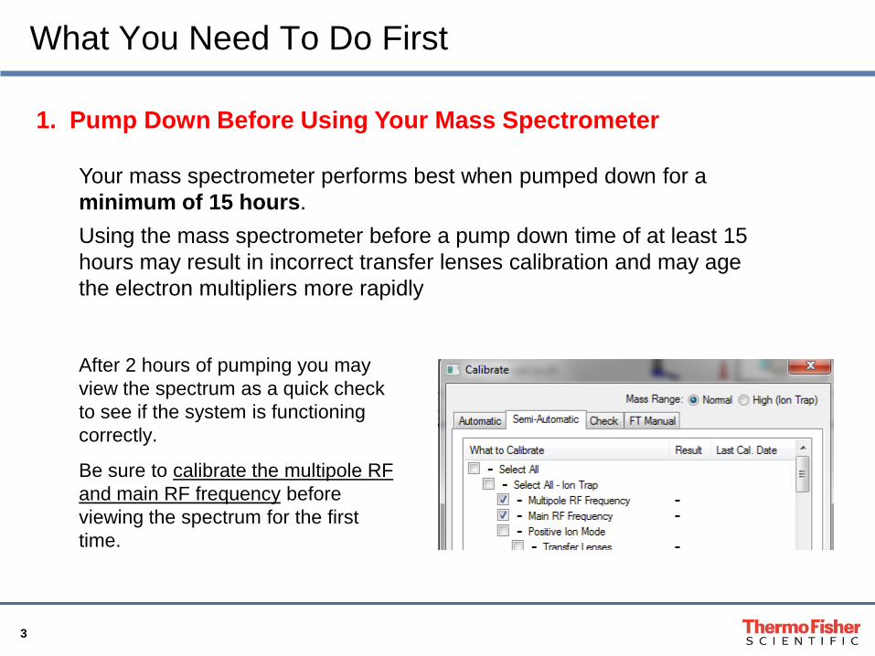
After 2 hours of pumping you may
view the spectrum as a quick check
to see if the system is functioning
correctly.
Be sure to calibrate the multipole RF
and main RF frequency before
viewing the spectrum for the first
time.
1. Pump Down Before Using Your Mass Spectrometer
Your mass spectrometer performs best when pumped down for a
minimum of 15 hours.
Using the mass spectrometer before a pump down time of at least 15
hours may result in incorrect transfer lenses calibration and may age
the electron multipliers more rapidly
4
What You Need To Do First
2. Install LTQ 2.7 SP1 or highest instrument control version
Using outdated versions of instrument control software may result in
reduced features and/or improper calibrations.
Always verify your instrument control software is up to date. You may
determine the latest version for your instrument from your FSE or sales
representative.
Call your sales representative or field service engineer to obtain the
latest version of your instrument‟s control software.
5
LTQ 2.7 SP1 and Sweep Gas
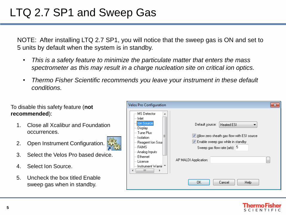
NOTE: After installing LTQ 2.7 SP1, you will notice that the sweep gas is ON and set to
5 units by default when the system is in standby.
• This is a safety feature to minimize the particulate matter that enters the mass
spectrometer as this may result in a charge nucleation site on critical ion optics.
• Thermo Fisher Scientific recommends you leave your instrument in these default
conditions.
To disable this safety feature (not
recommended):
1. Close all Xcalibur and Foundation
occurrences.
2. Open Instrument Configuration.
3. Select the Velos Pro based device.
4. Select Ion Source.
5. Uncheck the box titled Enable
sweep gas when in standby.
6
Information in this Guide:
• Section I: Ion Trap
• Achieving peak performance on the Velos Pro ion trap as a stand alone
instrument and as the front end for the Orbitrap Velos Pro and Orbitrap
Elite hybrid instruments.
• Section II: Orbitrap
• Achieving peak performance on the orbitrap portion of the Orbitrap Velos
Pro and Orbitrap Elite hybrid instruments.
Note: Most of this information is also pertinent to the LTQ Velos
and LTQ Orbitrap Velos mass spectrometers.

Section I: Ion Trap
Velos Pro Ion Optics
and Ion Trap
8
Section I Contents
1. Achieving and Maintaining a Stable Spray
2. Calibrating the Velos Pro
3. Tuning the Velos Pro for Optimal Performance
4. Diagnostics and Troubleshooting on the Velos Pro, Orbitrap Velos
Pro, and Orbitrap Elite
5. Cleaning the Ion Optics on the Velos Pro or the Velos Pro part of the
Orbitrap Velos Pro and Orbitrap Elite
6. Communicating with Thermo
9
1. Achieving and Maintaining a Stable Spray
• Prior to performing any experiment, tuning, calibration, or diagnostic
procedure, establishing a stable and consistent spray is essential.
• This is true for all source types, ESI, HESI, and NSI.
• Failure to maintain a stable spray will compromise the data quality or
result in a poor tune, failed calibration or diagnostic result.
• The goal is a spray with less than 15% RSD over at least 100 scans.
10
1. Achieving and Maintaining a Stable Spray
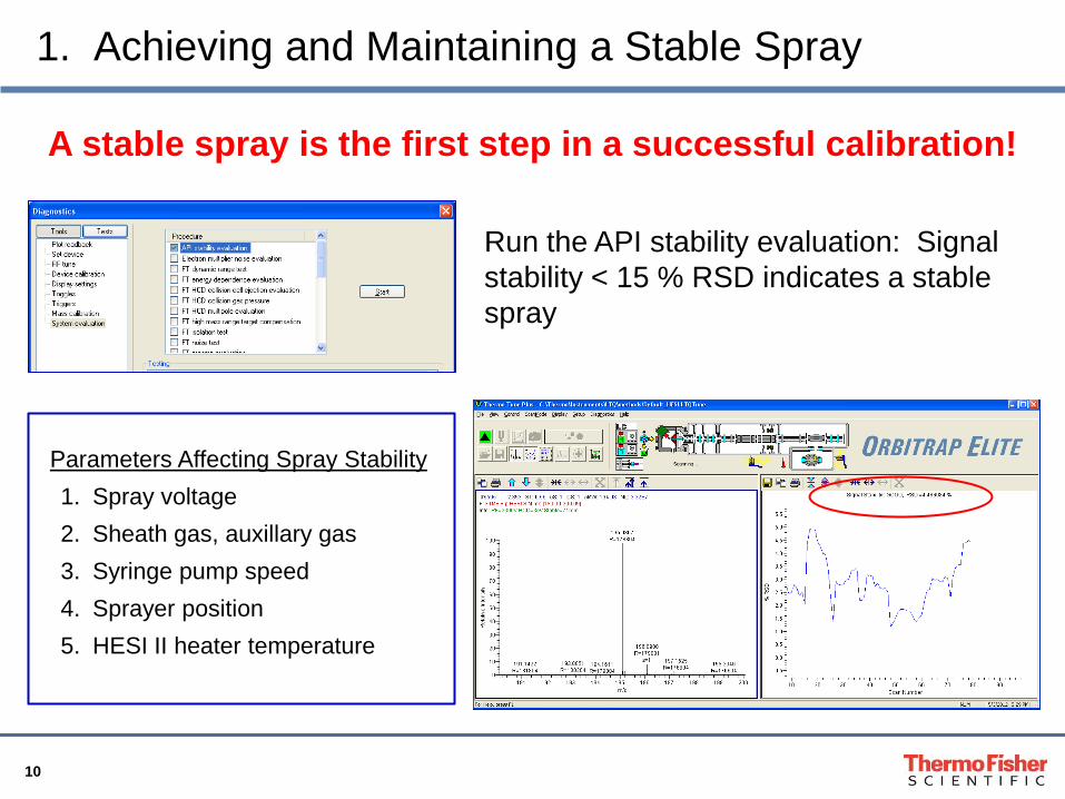
A stable spray is the first step in a successful calibration!
Run the API stability evaluation: Signal
stability < 15 % RSD indicates a stable
spray
Parameters Affecting Spray Stability
1. Spray voltage
2. Sheath gas, auxillary gas
3. Syringe pump speed
4. Sprayer position
5. HESI II heater temperature
11
1. Achieving and Maintaining a Stable Spray
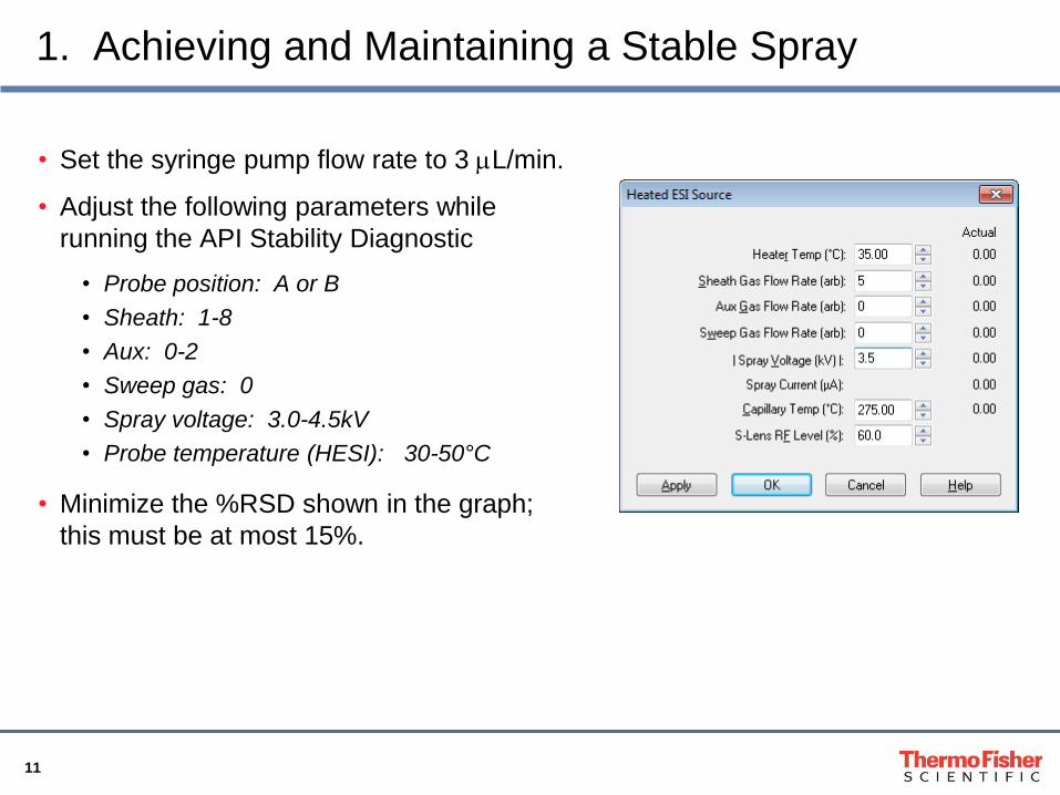
• Set the syringe pump flow rate to 3 mL/min.
• Adjust the following parameters while
running the API Stability Diagnostic
• Probe position: A or B
• Sheath: 1-8
• Aux: 0-2
• Sweep gas: 0
• Spray voltage: 3.0-4.5kV
• Probe temperature (HESI): 30-50°C
• Minimize the %RSD shown in the graph;
this must be at most 15%.
12
Section I Contents
1. Achieving and Maintaining a Stable Spray
2. Calibrating the Velos Pro
3. Tuning the Velos Pro for Optimal Performance
4. Diagnostics and Troubleshooting on the Velos Pro, Orbitrap Velos
Pro, and Orbitrap Elite
5. Cleaning the Ion Optics on the Velos Pro or the Velos Pro part of the
Orbitrap Velos Pro and Orbitrap Elite
13
2. Calibrating the Velos Pro
Key Starting Requirements:
1. Make sure that your instrument has been continuously under vacuum
for at least 15 hours since the last vent. Failure to do so may cause faulty
calibrations.
2. Install LTQ 2.7 SP1 or highest version available. Many of the key diagnostics
in this document are new to LTQ 2.7 SP1 and are not available in earlier
versions.
3. Ensure the spray is stable as described in 1. Achieving and Maintaining
a Stable Spray.
14
2. Calibrating the Velos Pro
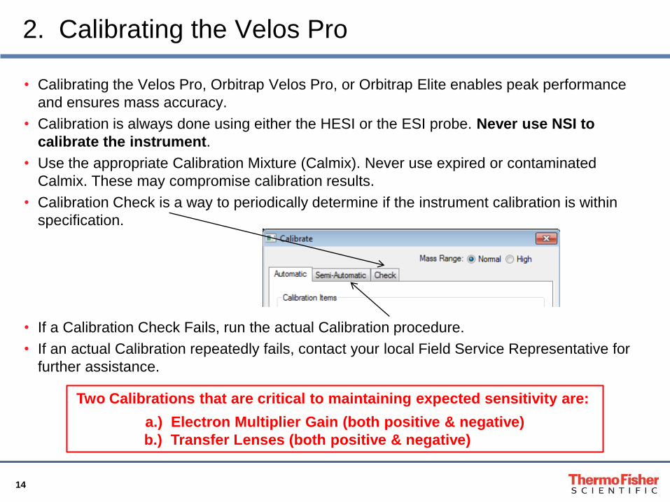
• Calibrating the Velos Pro, Orbitrap Velos Pro, or Orbitrap Elite enables peak performance
and ensures mass accuracy.
• Calibration is always done using either the HESI or the ESI probe. Never use NSI to
calibrate the instrument.
• Use the appropriate Calibration Mixture (Calmix). Never use expired or contaminated
Calmix. These may compromise calibration results.
• Calibration Check is a way to periodically determine if the instrument calibration is within
specification.
• If a Calibration Check Fails, run the actual Calibration procedure.
• If an actual Calibration repeatedly fails, contact your local Field Service Representative for
further assistance.
Two Calibrations that are critical to maintaining expected sensitivity are:
a.) Electron Multiplier Gain (both positive & negative)
b.) Transfer Lenses (both positive & negative)
15
2.a) Electron Multiplier Gain Calibration
• The gain will change more rapidly for new electron multipliers (either for new
instrument installations or replacements in older systems) versus older ones.
Consequently, the voltage necessary to maintain the correct gain will change
rapidly until a voltage plateau is reached.
• This effect is amplified in fast scanning instruments (e.g. LTQ (Orbitrap) Velos,
(Orbitrap) Velos Pro and Orbitrap Elite) due to the higher ion currents. The
graph on the next slide shows an example of the rate of voltage change for two
new electron multipliers in an LTQ Velos instrument.
• Typically a plateau is reached at operating voltages of approximately 900 to
1100 (ITT multipliers used in non-Pro instruments) or 1700 to1800 (SGE
multipliers used in Velos Pro, Orbitrap Velos Pro and Orbitrap Elite
instruments). Once the plateau is reached, the gain of the multipliers will
change more slowly, and therefore less frequent calibration is required.
• The time to reach the plateau will vary with instrument conditions and use –
electron multipliers in heavily used instruments will plateau faster than
instruments that are used only occasionally.
16
2.a) Electron Multiplier Gain Calibration
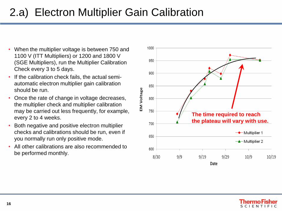
• When the multiplier voltage is between 750 and
1100 V (ITT Multipliers) or 1200 and 1800 V
(SGE Multipliers), run the Multiplier Calibration
Check every 3 to 5 days.
• If the calibration check fails, the actual semi-
automatic electron multiplier gain calibration
should be run.
• Once the rate of change in voltage decreases,
the multiplier check and multiplier calibration
may be carried out less frequently, for example,
every 2 to 4 weeks.
• Both negative and positive electron multiplier
checks and calibrations should be run, even if
you normally run only positive mode.
• All other calibrations are also recommended to
be performed monthly.
The time required to reach
the plateau will vary with use.
17
2.b) Transfer Lenses Calibration
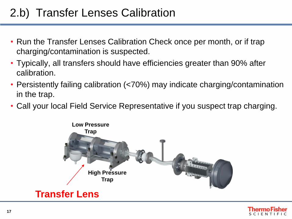
• Run the Transfer Lenses Calibration Check once per month, or if trap
charging/contamination is suspected.
• Typically, all transfers should have efficiencies greater than 90% after
calibration.
• Persistently failing calibration (<70%) may indicate charging/contamination
in the trap.
• Call your local Field Service Representative if you suspect trap charging.
High Pressure
Trap
Low Pressure
Trap
Transfer Lens
18
Section I Contents
1. Achieving and Maintaining a Stable Spray
2. Calibrating the Velos Pro
3. Tuning the Velos Pro for Optimal Performance
4. Diagnostics and Troubleshooting on the Velos Pro, Orbitrap Velos
Pro, and Orbitrap Elite
5. Cleaning the Ion Optics on the Velos Pro or the Velos Pro part of the
Orbitrap Velos Pro and Orbitrap Elite
6. Communicating with Thermo
19
3. Tuning the Velos Pro for Optimal Performance
Key Starting Requirements:
1. Ensure your instrument has been continuously under vacuum for at
least 15 hours since the last vent.
2. Install LTQ 2.7 SP1 or highest version available. Many of the key diagnostics
in this document are new to LTQ 2.7 SP1 and are not available in earlier
versions.
3. Ensure the spray is stable as described in 1. Achieving and Maintaining
a Stable Spray.
4. Verify all calibrations are up to date as described in 2. Calibrating the
Velos Pro.
20
3. Tuning the Velos Pro for Optimal Performance
• During the normal use of an instrument, sample/solvent residue will
accumulate on the components of the ion optics. Over time, the
accumulated residue can alter the tuning characteristics of the ion optics
components.
• Accumulated residue can result in sub-optimum tuning parameters.
This can be observed as a reduction in sensitivity. This reduction in
sensitivity can happen more rapidly if non-optimized tune values are
used, in addition to poor sample clean up and instrument usage.
• In order to obtain high levels of sensitivity over a longer period of time,
the ion optics must have an appropriate voltage gradient to resist
changes to tuning conditions due to usage.
21
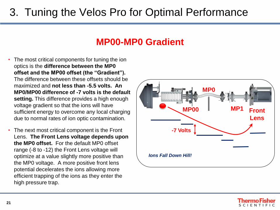
3. Tuning the Velos Pro for Optimal Performance
• The most critical components for tuning the ion
optics is the difference between the MP0
offset and the MP00 offset (the “Gradient”).
The difference between these offsets should be
maximized and not less than -5.5 volts. An
MP0/MP00 difference of -7 volts is the default
setting. This difference provides a high enough
voltage gradient so that the ions will have
sufficient energy to overcome any local charging
due to normal rates of ion optic contamination.
• The next most critical component is the Front
Lens. The Front Lens voltage depends upon
the MP0 offset. For the default MP0 offset
range (-8 to -12) the Front Lens voltage will
optimize at a value slightly more positive than
the MP0 voltage. A more positive front lens
potential decelerates the ions allowing more
efficient trapping of the ions as they enter the
high pressure trap.
-7 Volts
MP0
MP00 Front
Lens
MP00-MP0 Gradient
Ions Fall Down Hill!
MP1
22
3. Tuning the Velos Pro for Optimal Performance
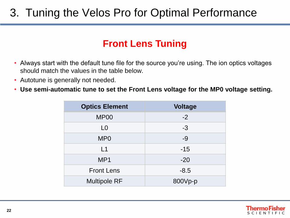
• Always start with the default tune file for the source you‟re using. The ion optics voltages
should match the values in the table below.
• Autotune is generally not needed.
• Use semi-automatic tune to set the Front Lens voltage for the MP0 voltage setting.
Optics Element Voltage
MP00 -2
L0 -3
MP0 -9
L1 -15
MP1 -20
Front Lens -8.5
Multipole RF 800Vp-p
Front Lens Tuning
23
3. Tuning the Velos Pro for Optimal Performance
-30 -28 -26 -24 -22 -20 -18 -16 -14 -12 -10 -8 -6 -4 -2 0 Lens Potential (V)
0
500000
1000000
1500000
2000000
2500000
3000000
3500000
4000000
TIC
-30 -28 -26 -24 -22 -20 -18 -16 -14 -12 -10 -8 -6 -4 -2 0 Lens Potential (V)
0
200000
400000
600000
800000
1000000
1200000
1400000
1600000
1800000
2000000
TIC
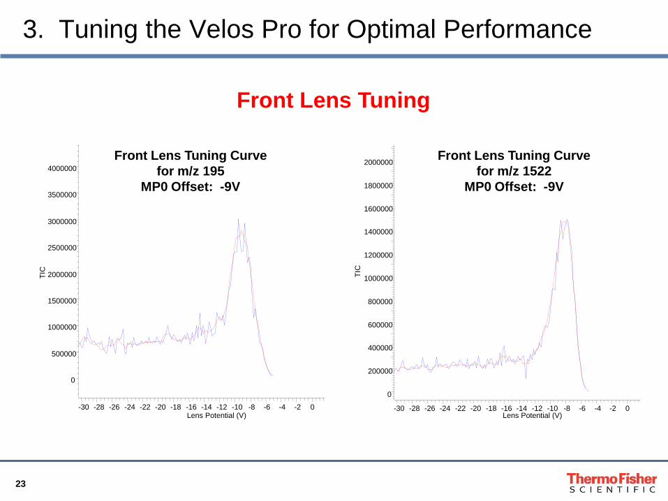
Front Lens Tuning Curve
for m/z 195
MP0 Offset: -9V
Front Lens Tuning Curve
for m/z 1522
MP0 Offset: -9V
Front Lens Tuning
24
3. Tuning the Velos Pro for Optimal Performance
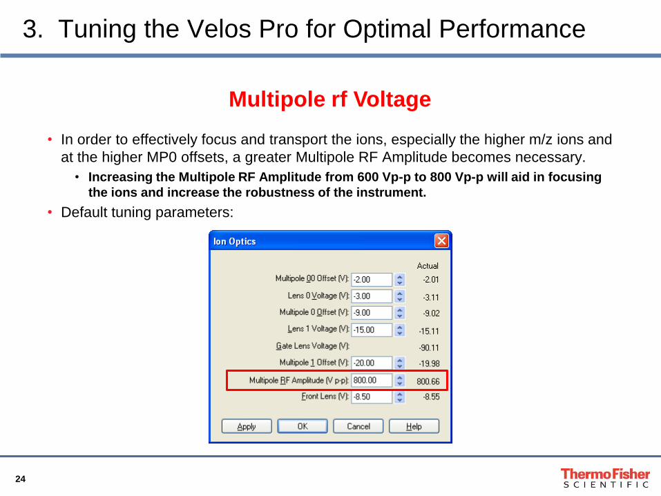
• In order to effectively focus and transport the ions, especially the higher m/z ions and
at the higher MP0 offsets, a greater Multipole RF Amplitude becomes necessary.
• Increasing the Multipole RF Amplitude from 600 Vp-p to 800 Vp-p will aid in focusing
the ions and increase the robustness of the instrument.
• Default tuning parameters:
Multipole rf Voltage
25
3. Tuning the Velos Pro for Optimal Performance
• Always use the released version of the instrument control software,
currently LTQ 2.7 SP1
• Earlier versions of instrument control software, for example LTQ 2.6.0
SP3, do not enforce the minimum MP00/MP0 difference. If your instrument
uses these earlier versions of instrument control software, upgrade your
instrument control software to LTQ 2.7 SP1.
26
3. Tuning the Velos Pro for Optimal Performance
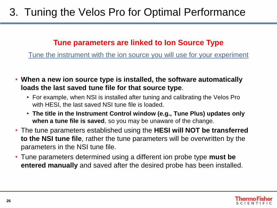
• When a new ion source type is installed, the software automatically
loads the last saved tune file for that source type.
• For example, when NSI is installed after tuning and calibrating the Velos Pro
with HESI, the last saved NSI tune file is loaded.
• The title in the Instrument Control window (e.g., Tune Plus) updates only
when a tune file is saved, so you may be unaware of the change.
• The tune parameters established using the HESI will NOT be transferred
to the NSI tune file, rather the tune parameters will be overwritten by the
parameters in the NSI tune file.
• Tune parameters determined using a different ion probe type must be
entered manually and saved after the desired probe has been installed.
Tune parameters are linked to Ion Source Type
Tune the instrument with the ion source you will use for your experiment
27
Section I Contents
1. Achieving and Maintaining a Stable Spray
2. Calibrating the Velos Pro
3. Tuning the Velos Pro for Optimal Performance
4. Diagnostics and Troubleshooting on the Velos Pro, Orbitrap
Velos Pro, and Orbitrap Elite: LTQ 2.7 SP1
5. Cleaning the Ion Optics on the Velos Pro or the Velos Pro part of the
Orbitrap Velos Pro and Orbitrap Elite
6. Communicating with Thermo
28
4. Troubleshooting and Diagnostics
• When following the standard operating procedure described in the
previous slides, your Velos Pro system should provide you with routine,
high performance results.
• However, you may occasionally be required to troubleshoot your
system in order to maintain optimum performance. To facilitate the
troubleshooting process, a number of system diagnostics have been
created in LTQ 2.7 SP1. These new diagnostics are described in the
remainder of this document.
29
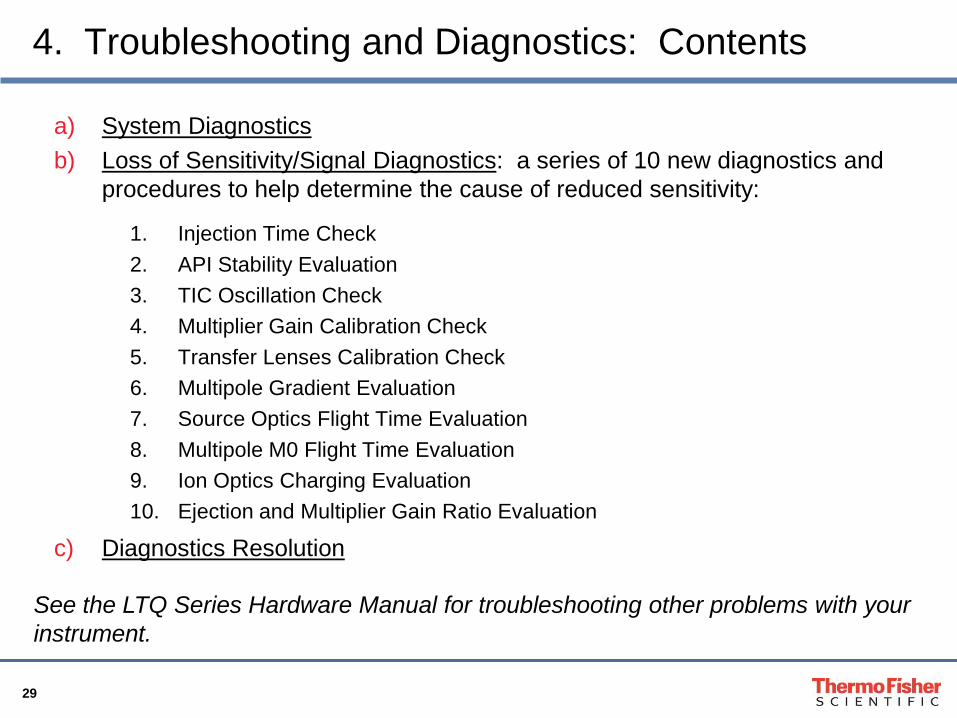
4. Troubleshooting and Diagnostics: Contents
a) System Diagnostics
b) Loss of Sensitivity/Signal Diagnostics: a series of 10 new diagnostics and
procedures to help determine the cause of reduced sensitivity:
1. Injection Time Check
2. API Stability Evaluation
3. TIC Oscillation Check
4. Multiplier Gain Calibration Check
5. Transfer Lenses Calibration Check
6. Multipole Gradient Evaluation
7. Source Optics Flight Time Evaluation
8. Multipole M0 Flight Time Evaluation
9. Ion Optics Charging Evaluation
10. Ejection and Multiplier Gain Ratio Evaluation
c) Diagnostics Resolution
See the LTQ Series Hardware Manual for troubleshooting other problems with your
instrument.
30
4. Troubleshooting and Diagnostics
Key Starting Requirements:
1. Make sure that your instrument has been continuously under vacuum for
at least 15 hours since the last vent.
2. Install LTQ 2.7 SP1 or highest version available. Many of the key diagnostics
in this document are new to LTQ 2.7 SP1 and are not available in earlier
versions.
3. Ensure the spray is stable as described in 1. Achieving and Maintaining
a Stable Spray.
4. Verify all calibrations are up to date as described in 2. Calibrating the
Velos Pro.
5. Ensure the tune parameters are set as described in 3: Tuning the Velos
Pro for Optimal Performance.
31
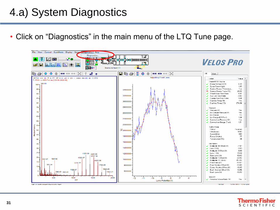
4.a) System Diagnostics
• Click on “Diagnostics” in the main menu of the LTQ Tune page.
32
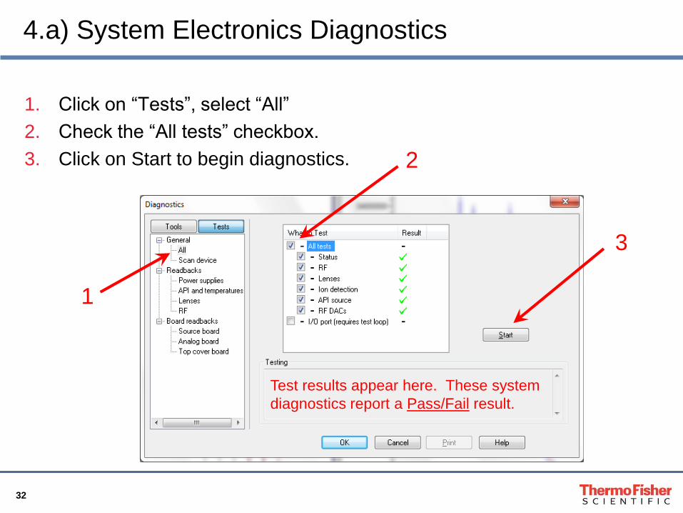
4.a) System Electronics Diagnostics
1. Click on “Tests”, select “All”
2. Check the “All tests” checkbox.
3. Click on Start to begin diagnostics.
1
2
3
Test results appear here. These system
diagnostics report a Pass/Fail result.
33
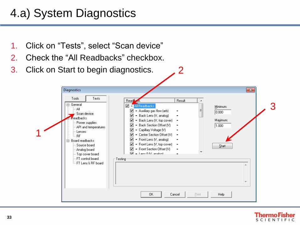
4.a) System Diagnostics
1. Click on “Tests”, select “Scan device”
2. Check the “All Readbacks” checkbox.
3. Click on Start to begin diagnostics.
1
2
3
34
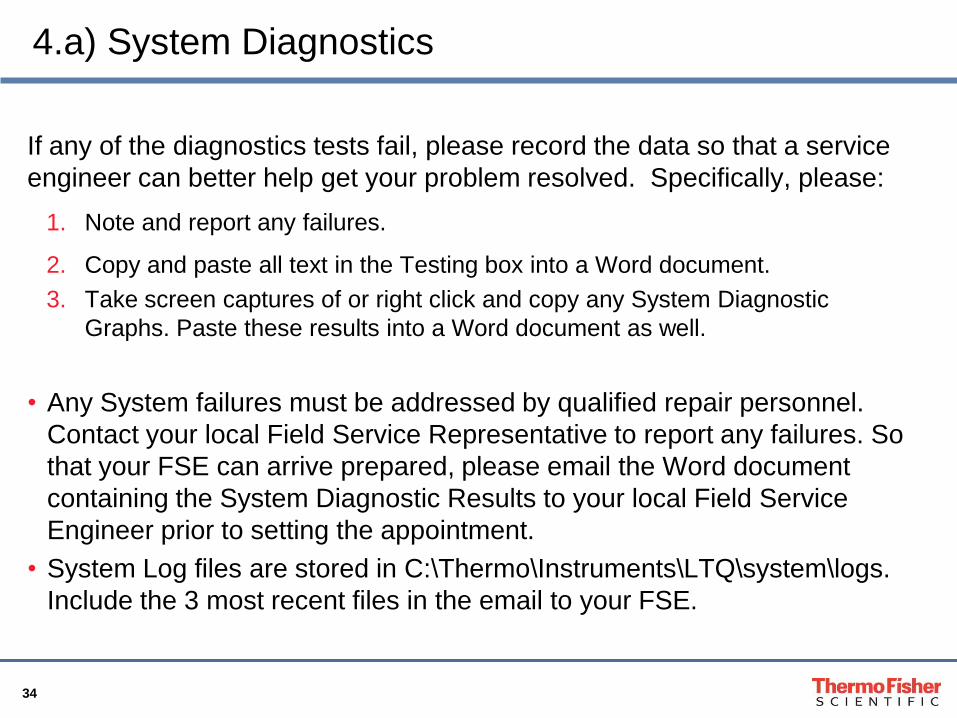
4.a) System Diagnostics
If any of the diagnostics tests fail, please record the data so that a service
engineer can better help get your problem resolved. Specifically, please:
1. Note and report any failures.
2. Copy and paste all text in the Testing box into a Word document.
3. Take screen captures of or right click and copy any System Diagnostic
Graphs. Paste these results into a Word document as well.
• Any System failures must be addressed by qualified repair personnel.
Contact your local Field Service Representative to report any failures. So
that your FSE can arrive prepared, please email the Word document
containing the System Diagnostic Results to your local Field Service
Engineer prior to setting the appointment.
• System Log files are stored in C:\Thermo\Instruments\LTQ\system\logs.
Include the 3 most recent files in the email to your FSE.
35
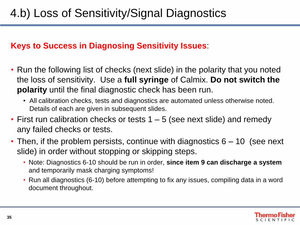
4.b) Loss of Sensitivity/Signal Diagnostics
Keys to Success in Diagnosing Sensitivity Issues:
• Run the following list of checks (next slide) in the polarity that you noted
the loss of sensitivity. Use a full syringe of Calmix. Do not switch the
polarity until the final diagnostic check has been run.
• All calibration checks, tests and diagnostics are automated unless otherwise noted.
Details of each are given in subsequent slides.
• First run calibration checks or tests 1 – 5 (see next slide) and remedy
any failed checks or tests.
• Then, if the problem persists, continue with diagnostics 6 – 10 (see next
slide) in order without stopping or skipping steps.
• Note: Diagnostics 6-10 should be run in order, since item 9 can discharge a system
and temporarily mask charging symptoms!
• Run all diagnostics (6-10) before attempting to fix any issues, compiling data in a word
document throughout.
36
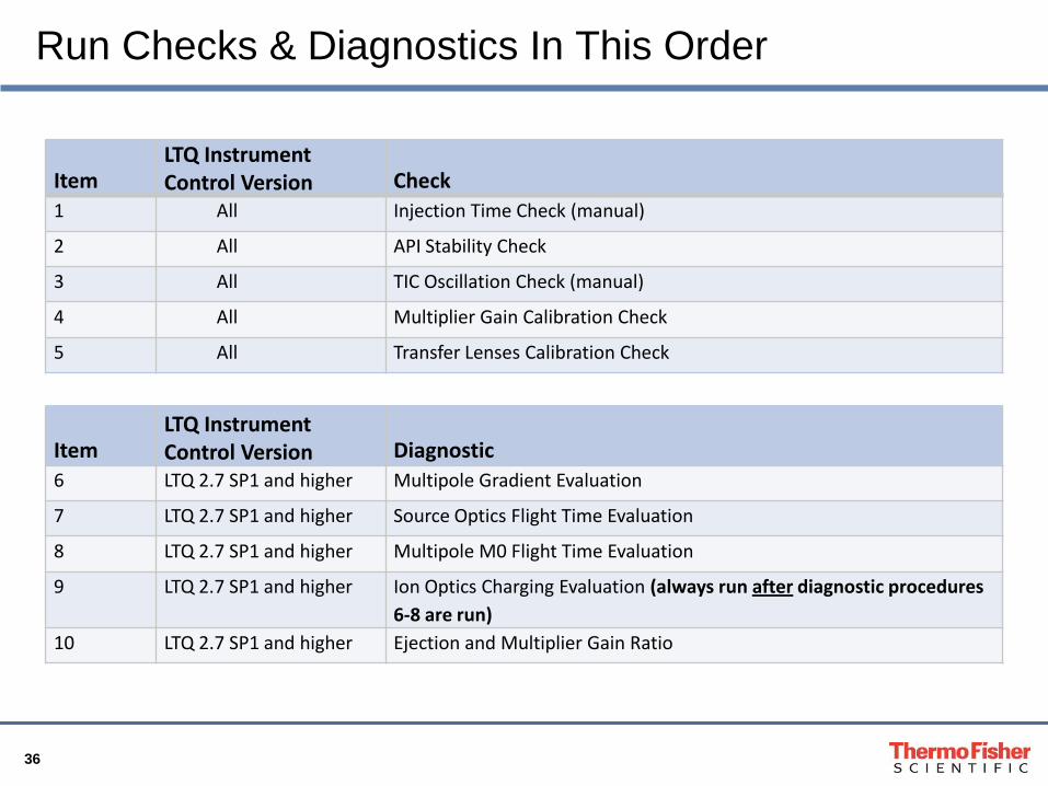
Run Checks & Diagnostics In This Order
Item LTQ Instrument Control Version Check
1 All Injection Time Check (manual)
2 All API Stability Check
3 All TIC Oscillation Check (manual)
4 All Multiplier Gain Calibration Check
5 All Transfer Lenses Calibration Check
Item LTQ Instrument Control Version Diagnostic
6 LTQ 2.7 SP1 and higher Multipole Gradient Evaluation
7 LTQ 2.7 SP1 and higher Source Optics Flight Time Evaluation
8 LTQ 2.7 SP1 and higher Multipole M0 Flight Time Evaluation
9 LTQ 2.7 SP1 and higher Ion Optics Charging Evaluation (always run after diagnostic procedures
6-8 are run)
10 LTQ 2.7 SP1 and higher Ejection and Multiplier Gain Ratio
37
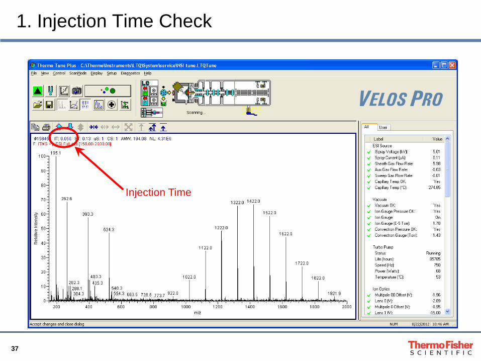
1. Injection Time Check
Injection Time
38
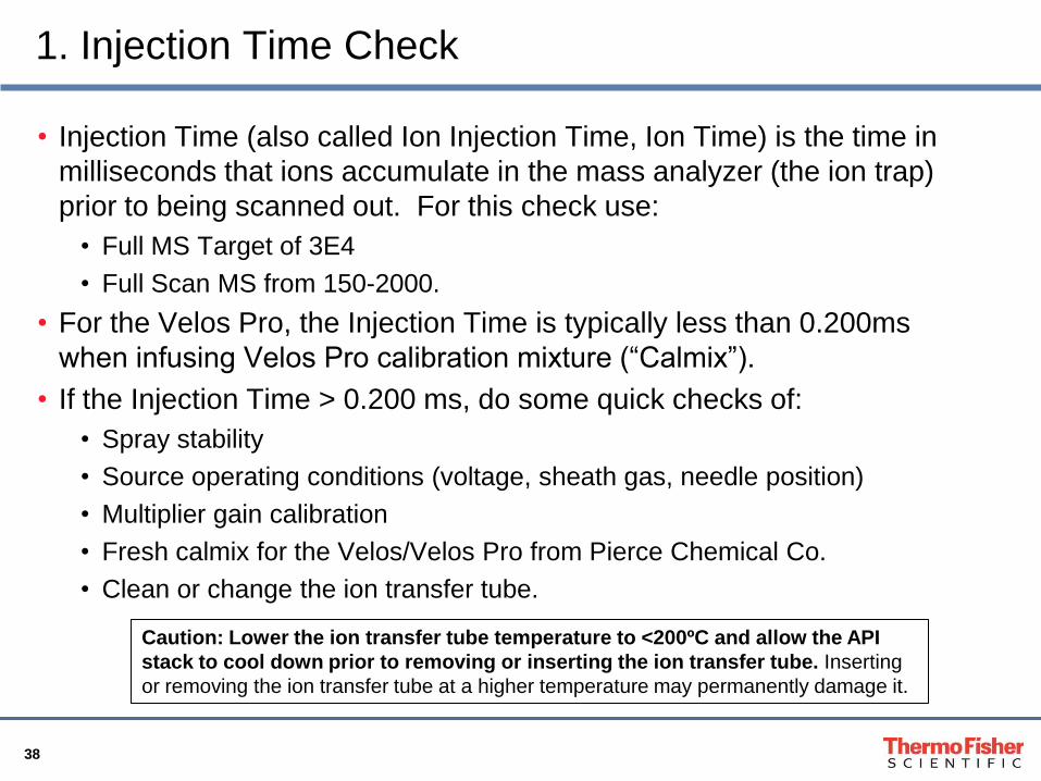
1. Injection Time Check
• Injection Time (also called Ion Injection Time, Ion Time) is the time in
milliseconds that ions accumulate in the mass analyzer (the ion trap)
prior to being scanned out. For this check use:
• Full MS Target of 3E4
• Full Scan MS from 150-2000.
• For the Velos Pro, the Injection Time is typically less than 0.200ms
when infusing Velos Pro calibration mixture (“Calmix”).
• If the Injection Time > 0.200 ms, do some quick checks of:
• Spray stability
• Source operating conditions (voltage, sheath gas, needle position)
• Multiplier gain calibration
• Fresh calmix for the Velos/Velos Pro from Pierce Chemical Co.
• Clean or change the ion transfer tube.
Caution: Lower the ion transfer tube temperature to <200ºC and allow the API
stack to cool down prior to removing or inserting the ion transfer tube. Inserting
or removing the ion transfer tube at a higher temperature may permanently damage it.
39
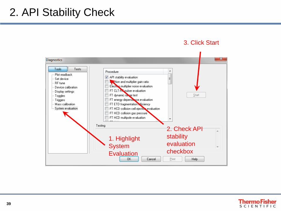
2. API Stability Check
1. Highlight
System
Evaluation
2. Check API
stability
evaluation
checkbox
3. Click Start
40
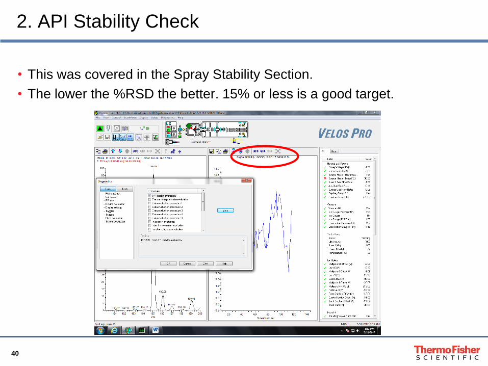
2. API Stability Check
• This was covered in the Spray Stability Section.
• The lower the %RSD the better. 15% or less is a good target.
41
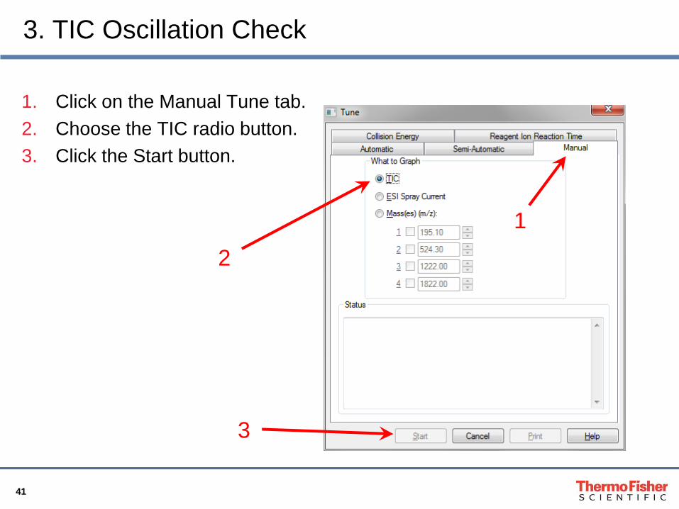
3. TIC Oscillation Check
1. Click on the Manual Tune tab.
2. Choose the TIC radio button.
3. Click the Start button.
1
2
3
42
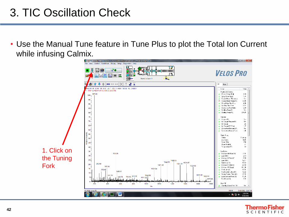
3. TIC Oscillation Check
• Use the Manual Tune feature in Tune Plus to plot the Total Ion Current
while infusing Calmix.
1. Click on
the Tuning
Fork
43
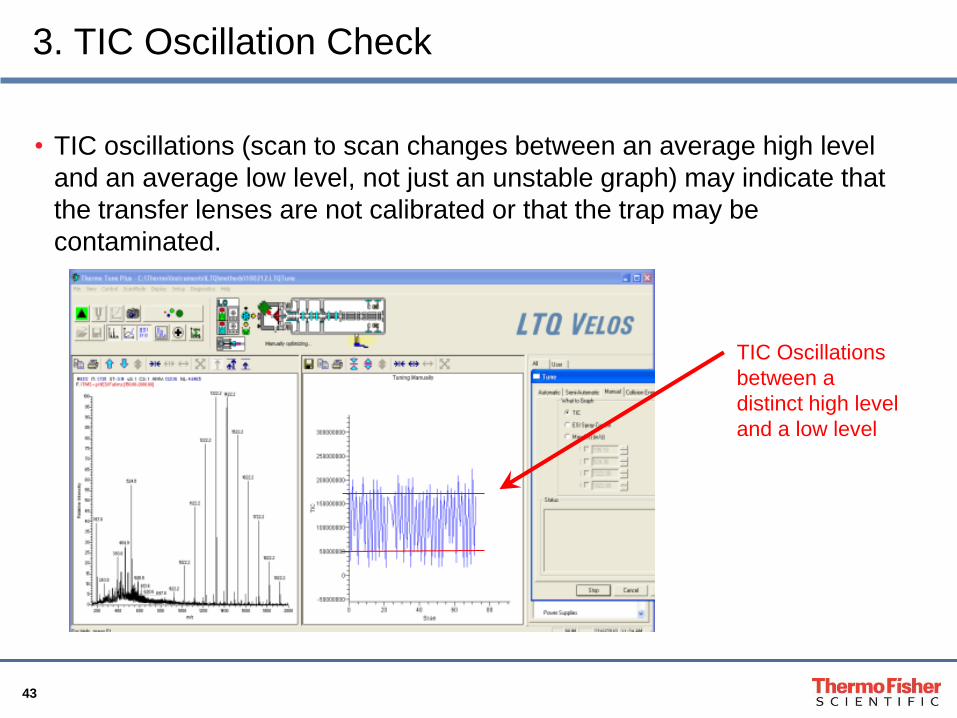
3. TIC Oscillation Check
• TIC oscillations (scan to scan changes between an average high level
and an average low level, not just an unstable graph) may indicate that
the transfer lenses are not calibrated or that the trap may be
contaminated.
TIC Oscillations
between a
distinct high level
and a low level
44
3. TIC Oscillation Check
• If the TIC Oscillates
• Run the Multiplier Gain Check (next section)
• Run the Transfer Lens Calibration Check
• Run the Multiplier Gain Calibration, if necessary
• Run Transfer Lens Calibration
• If the problem persists, the ion trap may be charging. Take screen captures
or make a raw file of your observations to share with your local field service
representative.
All ion trap work must be done by a
qualified Field Service Representative
45
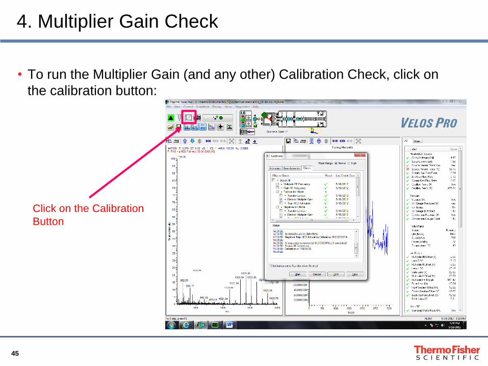
4. Multiplier Gain Check
• To run the Multiplier Gain (and any other) Calibration Check, click on
the calibration button:
Click on the Calibration
Button
46
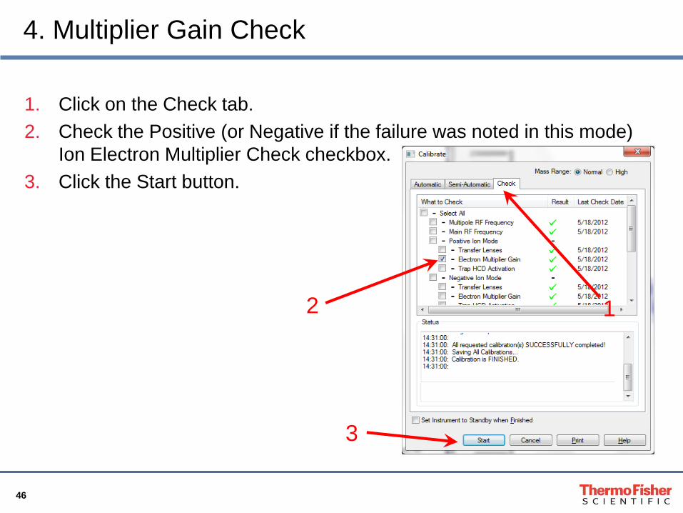
4. Multiplier Gain Check
1. Click on the Check tab.
2. Check the Positive (or Negative if the failure was noted in this mode)
Ion Electron Multiplier Check checkbox.
3. Click the Start button.
1 2
3

47
4. Multiplier Gain Check
• If the Multiplier Gain Check Fails
• Run the Multiplier Gain Calibration.
• The Multiplier Gain Check, and if needed the Multiplier Gain Calibration,
should be run on a weekly basis regardless of loss of signal. See the
section on Calibration above.
• If the Multiplier Gain Calibration fails, make sure the spray is stable.
Repeated failures with a stable spray suggests a Field Service call is in
order.
• Be sure to take screen shots of all results, including all of the calibration
text, and email these data to your local Field Service Representative.
48
4. Multiplier Gain Check
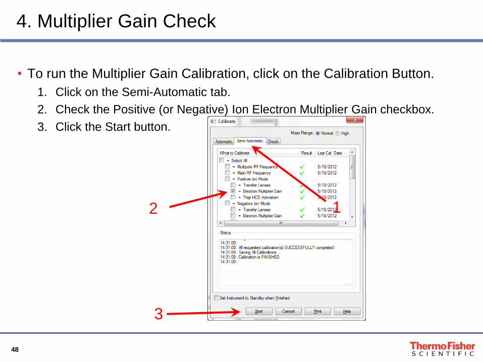
• To run the Multiplier Gain Calibration, click on the Calibration Button.
1. Click on the Semi-Automatic tab.
2. Check the Positive (or Negative) Ion Electron Multiplier Gain checkbox.
3. Click the Start button.
1 2
3
49
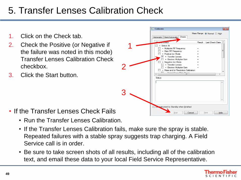
5. Transfer Lenses Calibration Check
1. Click on the Check tab.
2. Check the Positive (or Negative if
the failure was noted in this mode)
Transfer Lenses Calibration Check
checkbox.
3. Click the Start button.
1
2
3
• If the Transfer Lenses Check Fails
• Run the Transfer Lenses Calibration.
• If the Transfer Lenses Calibration fails, make sure the spray is stable.
Repeated failures with a stable spray suggests trap charging. A Field
Service call is in order.
• Be sure to take screen shots of all results, including all of the calibration
text, and email these data to your local Field Service Representative.
50
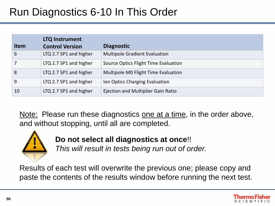
Run Diagnostics 6-10 In This Order
Item LTQ Instrument Control Version Diagnostic
6 LTQ 2.7 SP1 and higher Multipole Gradient Evaluation
7 LTQ 2.7 SP1 and higher Source Optics Flight Time Evaluation
8 LTQ 2.7 SP1 and higher Multipole M0 Flight Time Evaluation
9 LTQ 2.7 SP1 and higher Ion Optics Charging Evaluation
10 LTQ 2.7 SP1 and higher Ejection and Multiplier Gain Ratio
Note: Please run these diagnostics one at a time, in the order above,
and without stopping, until all are completed.
Do not select all diagnostics at once!!
This will result in tests being run out of order.
Results of each test will overwrite the previous one; please copy and
paste the contents of the results window before running the next test.
51
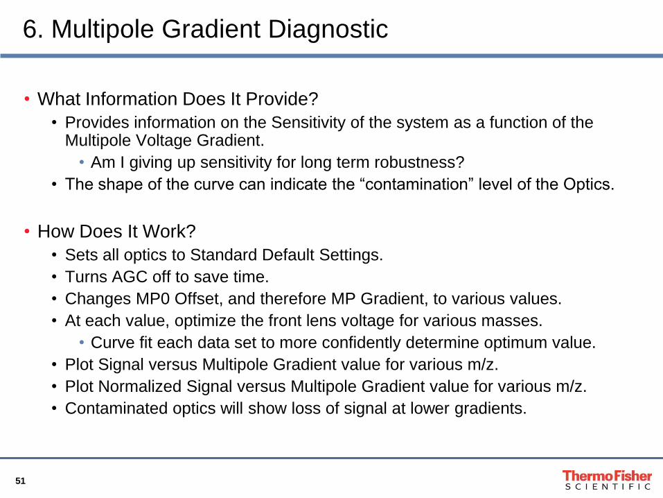
6. Multipole Gradient Diagnostic
• What Information Does It Provide?
• Provides information on the Sensitivity of the system as a function of the Multipole Voltage Gradient.
• Am I giving up sensitivity for long term robustness?
• The shape of the curve can indicate the “contamination” level of the Optics.
• How Does It Work?
• Sets all optics to Standard Default Settings.
• Turns AGC off to save time.
• Changes MP0 Offset, and therefore MP Gradient, to various values.
• At each value, optimize the front lens voltage for various masses.
• Curve fit each data set to more confidently determine optimum value.
• Plot Signal versus Multipole Gradient value for various m/z.
• Plot Normalized Signal versus Multipole Gradient value for various m/z.
• Contaminated optics will show loss of signal at lower gradients.
52
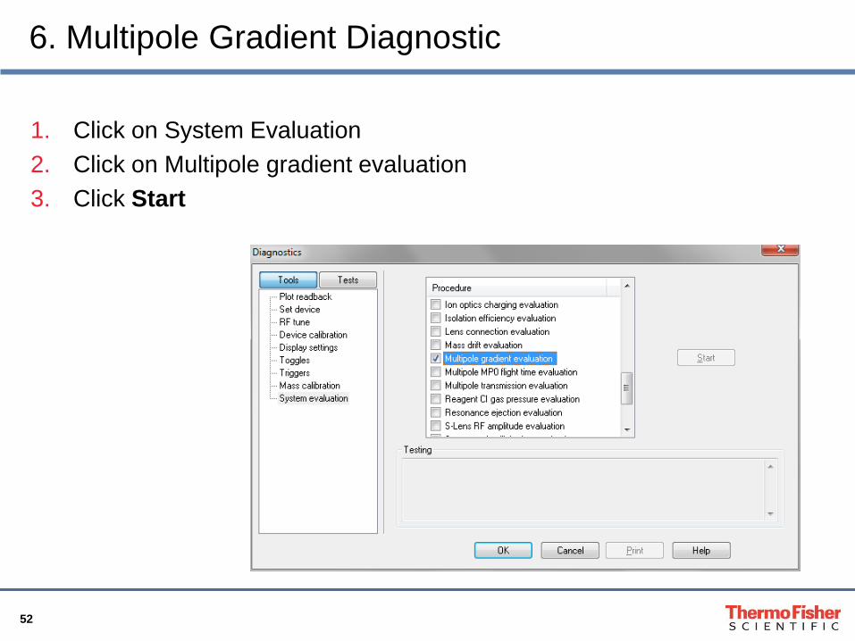
6. Multipole Gradient Diagnostic
1. Click on System Evaluation
2. Click on Multipole gradient evaluation
3. Click Start
53
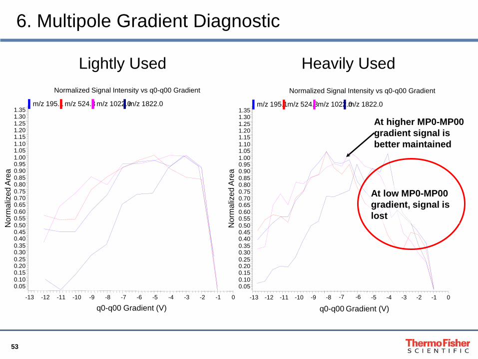
6. Multipole Gradient Diagnostic
Normalized Signal Intensity vs q0-q00 Gradient
-13 -12 -11 -10 -9 -8 -7 -6 -5 -4 -3 -2 -1 0
q0-q00 Gradient (V)
m/z 195.1 m/z 524.3 m/z 1022.0 m/z 1822.0
0.05 0.10 0.15 0.20 0.25 0.30 0.35 0.40 0.45 0.50 0.55 0.60 0.65 0.70 0.75 0.80 0.85 0.90 0.95 1.00 1.05 1.10
1.15 1.20 1.25 1.30 1.35
Norm
aliz
ed
Are
a
Normalized Signal Intensity vs q0-q00 Gradient
-13 -12 -11 -10 -9 -8 -5 -4 -3 -2 -1 0
q0-q00 Gradient (V)
m/z 195.1 m/z 524.3 m/z 1022.0 m/z 1822.0
0.05 0.10 0.15 0.20 0.25 0.30 0.35 0.40 0.45 0.50 0.55 0.60 0.65 0.70 0.75 0.80 0.85 0.90 0.95 1.00 1.05 1.10 1.15 1.20 1.25 1.30 1.35
No
rma
lize
d A
rea
At higher MP0-MP00
gradient signal is
better maintained
-7 -6
At low MP0-MP00
gradient, signal is
lost
Lightly Used Heavily Used
54
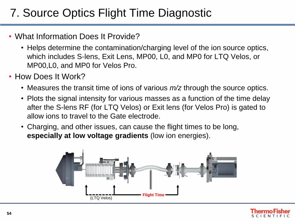
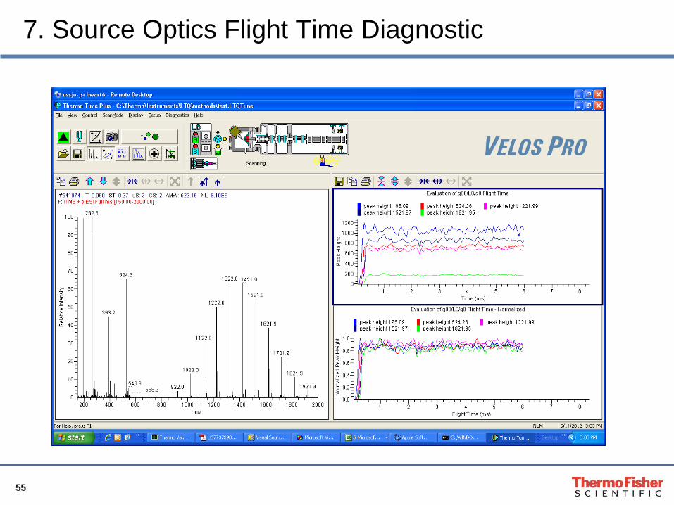
7. Source Optics Flight Time Diagnostic
• What Information Does It Provide?
• Helps determine the contamination/charging level of the ion source optics,
which includes S-lens, Exit Lens, MP00, L0, and MP0 for LTQ Velos, or
MP00,L0, and MP0 for Velos Pro.
• How Does It Work?
• Measures the transit time of ions of various m/z through the source optics.
• Plots the signal intensity for various masses as a function of the time delay
after the S-lens RF (for LTQ Velos) or Exit lens (for Velos Pro) is gated to
allow ions to travel to the Gate electrode.
• Charging, and other issues, can cause the flight times to be long,
especially at low voltage gradients (low ion energies).
Flight Time (LTQ Velos)
55
7. Source Optics Flight Time Diagnostic
56
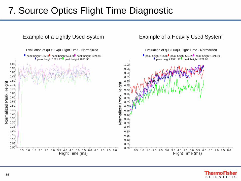
7. Source Optics Flight Time Diagnostic
0.5 1.0 1.5 2.0 2.5 3.0 3.5 4.0 4.5 5.0 5.5 6.0 6.5 7.0 7.5 8.0
Flight Time (ms)
0.00
0.05
0.10
0.15
0.20
0.25
0.30
0.35
0.40
0.45
0.50
0.55
0.60
0.65
0.70
0.75
0.80
0.85
0.90
0.95
1.00
No
rma
lize
d P
ea
k H
eig
ht
0.5 1.0 1.5 2.0 2.5 3.0 3.5 4.0 4.5 5.0 5.5 6.0 6.5 7.0 7.5 8.0
Flight Time (ms)
0.00
0.05
0.10
0.15
0.20
0.25
0.30
0.35
0.40
0.45
0.50
0.55
0.60
0.65
0.70
0.75
0.80
0.85
0.90
0.95
1.00
Norm
aliz
ed
Pe
ak H
eig
ht
peak height 195.09 peak height 524.26 peak height 1221.99
peak height 1521.97 peak height 1821.95
Evaluation of q00/L0/q0 Flight Time - Normalized
Example of a Lightly Used System Example of a Heavily Used System
peak height 195.09 peak height 524.26 peak height 1221.99
peak height 1521.97 peak height 1821.95
Evaluation of q00/L0/q0 Flight Time - Normalized
57
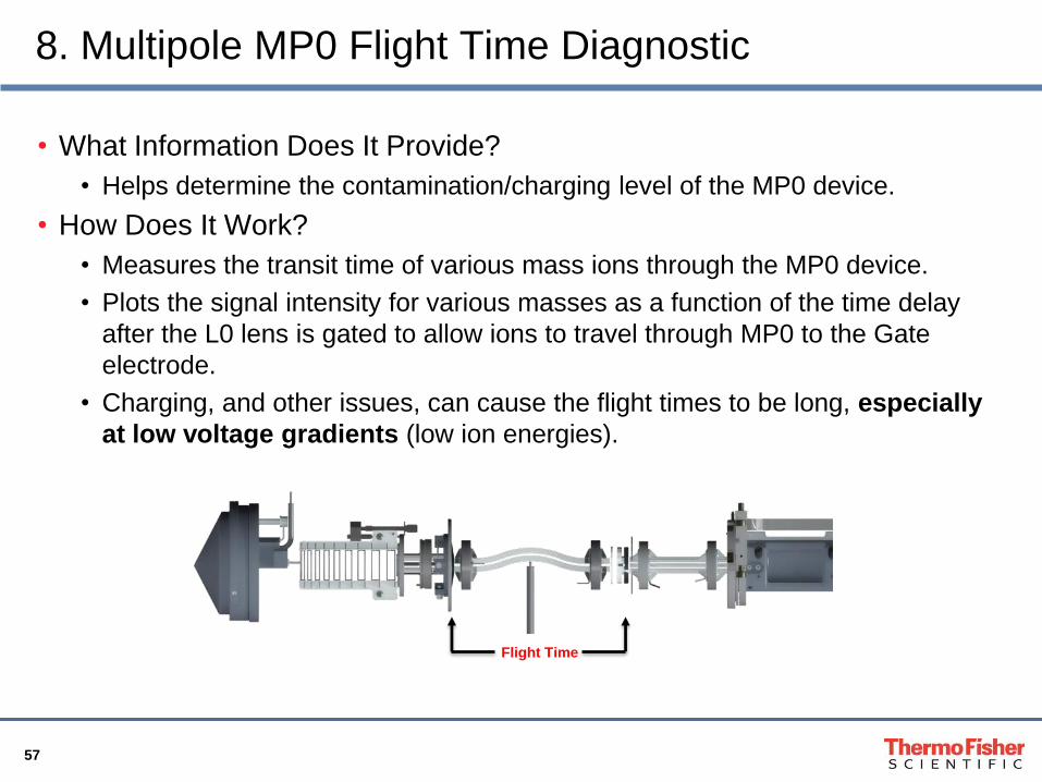
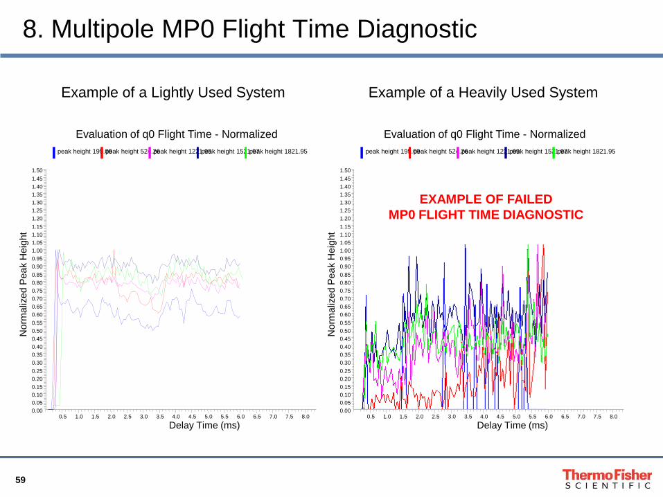
8. Multipole MP0 Flight Time Diagnostic
• What Information Does It Provide?
• Helps determine the contamination/charging level of the MP0 device.
• How Does It Work?
• Measures the transit time of various mass ions through the MP0 device.
• Plots the signal intensity for various masses as a function of the time delay
after the L0 lens is gated to allow ions to travel through MP0 to the Gate
electrode.
• Charging, and other issues, can cause the flight times to be long, especially
at low voltage gradients (low ion energies).
Flight Time
58
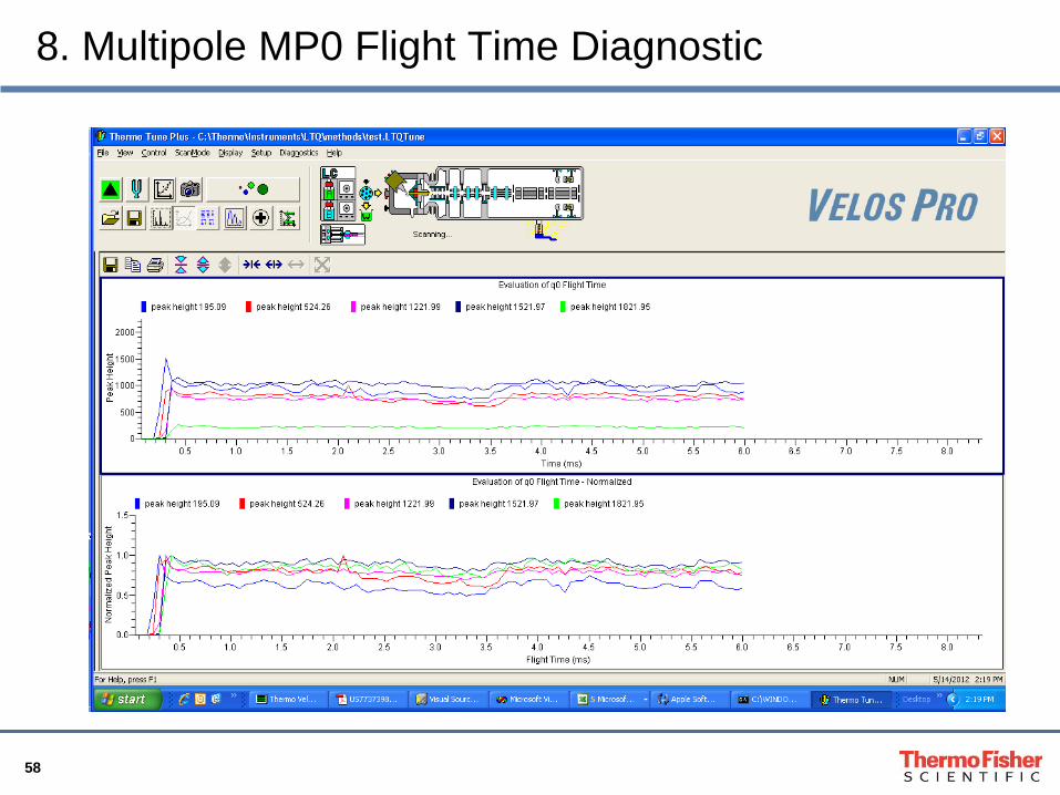
8. Multipole MP0 Flight Time Diagnostic
59
8. Multipole MP0 Flight Time Diagnostic
0.5 1.0 1.5 2.0 2.5 3.0 3.5 4.0 4.5 5.0 5.5 6.0 6.5 7.0 7.5 8.0
Delay Time (ms)
0.00
0.05
0.10
0.15
0.20
0.25
0.30
0.35
0.40
0.45
0.50
0.55
0.60
0.65
0.70
0.75
0.80
0.85
0.90
0.95
1.00
1.05
1.10
1.15
1.20
1.25
1.30
1.35
1.40
1.45
1.50
No
rma
lize
d P
ea
k H
eig
ht
Evaluation of q0 Flight Time - Normalized
peak height 195.09 peak height 524.26 peak height 1221.99 peak height 1521.97 peak height 1821.95
Example of a Lightly Used System Example of a Heavily Used System
EXAMPLE OF FAILED
MP0 FLIGHT TIME DIAGNOSTIC
60
9. Ion Optics Charging Diagnostic
• What Information Does It Provide?
• Helps to Identify which Ion Optic Components are Charging
• Helps Identify which parts may need to be cleaned
• How Does It Work?
• Sequentially tests each optical element
• Plots positive Ion TIC for 30 sec
• Switches to Negative Polarity and transmits negative ion beam (100 ms Injection times) for 80 seconds up to the ion optical element being tested
• Switches back to Positive Ion Polarity and Continues Plotting positive Ion TIC for 30 sec
• If the element is charged, a spike in the intensity will be observed after exposure to negative ions
• Plot Post/Pre Negative Ion Exposure Intensity Ratios for various mass window.
• Discharging process is usually very m/z dependant
• Measures Pos Ion/Neg Ion Flux Ratio, since this can directly effect the results
• Common reasons for low Neg Ion Flux
Never Calibrated – Gain and Transfer Lens
Never Tuned for Negative Ions
Sheath Gas not appropriate for Neg Ions
• Scans are in Turbo Scan Rate to save time
• Note that once this diagnostic is run, it can discharge the system. Consequently, running it a second time may not show the same behavior.
61
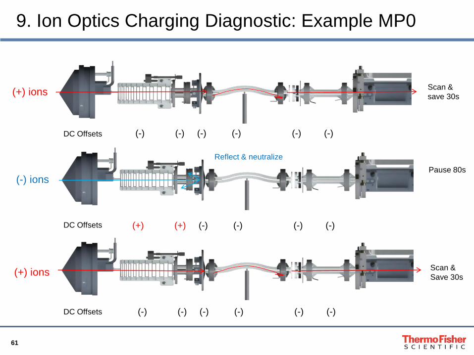
9. Ion Optics Charging Diagnostic: Example MP0
(+) ions
(+) ions
(-) ions
DC Offsets
DC Offsets
DC Offsets
(-) (-) (-) (-) (-) (-)
(+) (+) (-) (-) (-) (-)
(-) (-) (-) (-) (-) (-)
Scan &
save 30s
Scan &
Save 30s
Pause 80s
Reflect & neutralize
62
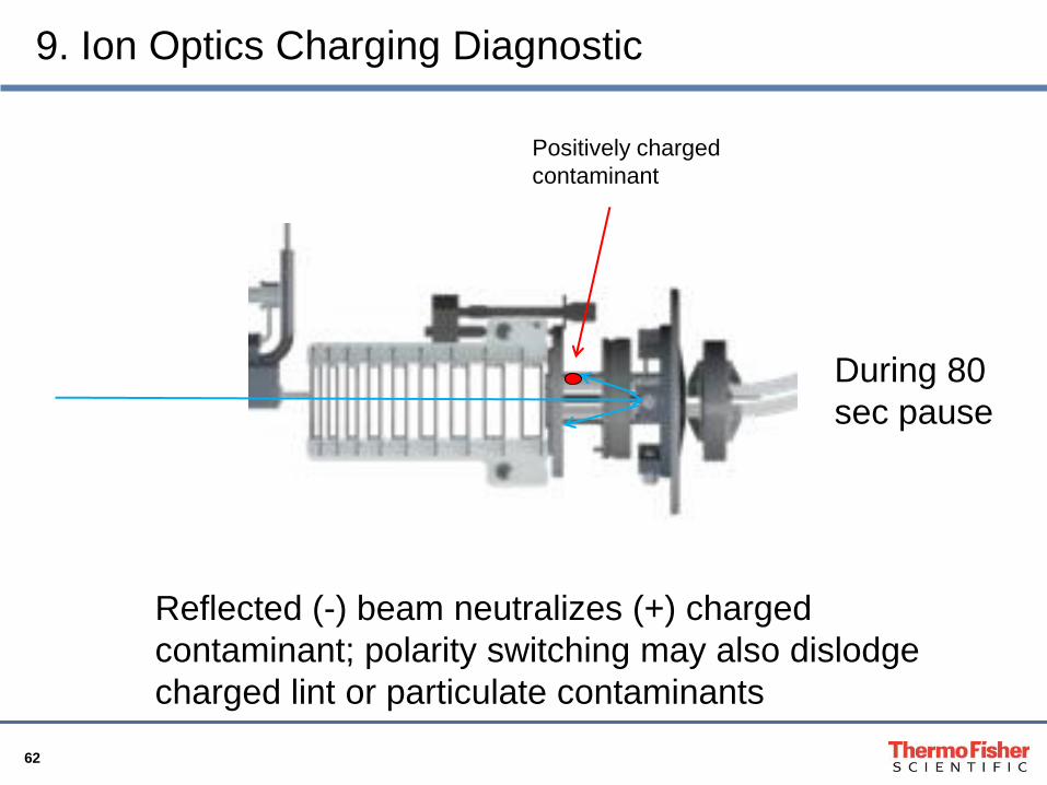
9. Ion Optics Charging Diagnostic
Reflected (-) beam neutralizes (+) charged
contaminant; polarity switching may also dislodge
charged lint or particulate contaminants
Positively charged
contaminant
During 80
sec pause
63
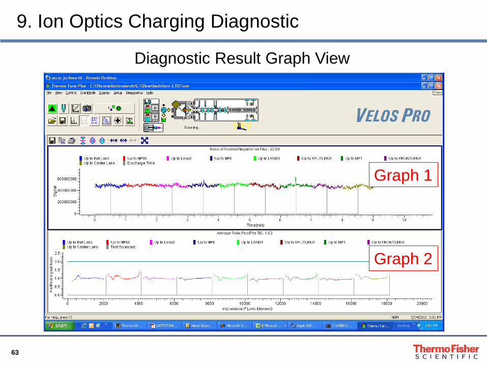
9. Ion Optics Charging Diagnostic
Graph 1
Graph 2
Diagnostic Result Graph View
64
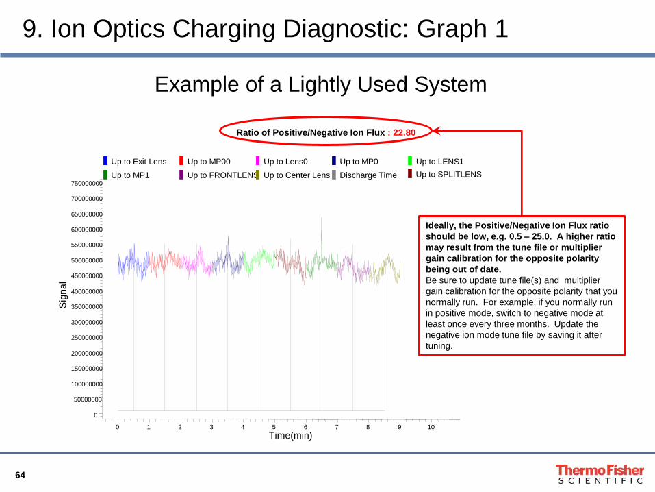
Ratio of Positive/Negative Ion Flux : 22.80
0 1 2 3 4 5 6 7 8 9 10
Time(min)
Up to Exit Lens Up to MP00 Up to Lens0 Up to MP0 Up to LENS1
Up to SPLITLENS Up to MP1 Up to FRONTLENS Up to Center Lens Discharge Time
0
50000000
100000000
150000000
200000000
250000000
300000000
350000000
400000000
450000000
500000000
550000000
600000000
650000000
700000000
750000000
Sig
na
l
Ideally, the Positive/Negative Ion Flux ratio
should be low, e.g. 0.5 – 25.0. A higher ratio
may result from the tune file or multiplier
gain calibration for the opposite polarity
being out of date.
Be sure to update tune file(s) and multiplier
gain calibration for the opposite polarity that you
normally run. For example, if you normally run
in positive mode, switch to negative mode at
least once every three months. Update the
negative ion mode tune file by saving it after
tuning.
9. Ion Optics Charging Diagnostic: Graph 1
Example of a Lightly Used System

65
Example of a Lightly Used System
m/z window (* Lens Element)
Average Ratio Post/Pre TIC: 1.03
0 2000 4000 6000 8000 10000 12000 14000 16000 18000 20000
Up to Exit Lens Up to MP00 Up to Lens0 Up to MP0 Up to LENS1 Up to SPLITLENS Up to MP1 Up to FRONTLENS Up to Center Lens Test Boundary
-0.1
0.0
0.1
0.2
0.3
0.4
0.5
0.6
0.7
0.8
0.9
1.0
1.1
1.2
1.3
1.4
1.5
1.6
1.7
1.8
1.9
2.0
2.1
2.2
2.3
2.4
2.5
Pre
/Post S
ignal R
atio
Failure
Threshold (2X)
Axis represents
Cumulative Mass Range
0-2000 for each Optic
9. Ion Optics Charging Diagnostic: Graph 2
0-2000
Exit
Lens
0-2000
MP00
0-2000
Lens 0
0-2000
Lens 1
0-2000
MP1
0-2000
Centre
Lens
0-2000
MP0
0-2000
Split
Lens
0-2000
Gate
Lens

66
9. Ion Optics Charging Diagnostic: Exit Lens Charging
Ratio of Positive/Negative Ion Flux : 20.30
-0.5 0.0 0.5 1.0 1.5 2.0 2.5 3.0 3.5 4.0 4.5 5.0 5.5 6.0 6.5 7.0 7.5 8.0 8.5 9.0
Time(min)
Up to Exit Lens Up to MP00 Up to Lens0 Up to MP0 Up to LENS1 Up to SPLITLENS
Up to MP1 Up to FRONTLENS Up to Center Lens Discharge Time
0
10000000
20000000
30000000
40000000
50000000
60000000
70000000
80000000
90000000
100000000
110000000
120000000
130000000
140000000
150000000
160000000
170000000
180000000
190000000
Sig
na
l
Average Ratio Post/Pre TIC: 1.11
0 2000 4000 6000 8000 10000 12000 14000 16000 18000
m/z window (* Lens Element)
Up to Exit Lens Up to MP00 Up to Lens0 Up to MP0 Up to LENS1 Up to SPLITLENS
Up to MP1 Up to FRONTLENS Up to Center Lens Test Boundary
0.0
0.1
0.2
0.3
0.4
0.5
0.6
0.7
0.8
0.9
1.0
1.1
1.2
1.3
1.4
1.5
1.6
1.7
1.8
1.9
2.0
2.1
2.2
2.3
Pre
/Po
st S
ign
al R
atio
Example of Heavily Used System
with Exit Lens Charging
Above Threshold
Indicates Exit Lens Charging
Instability in Signal
Indicates Exit
Lens Charging
67
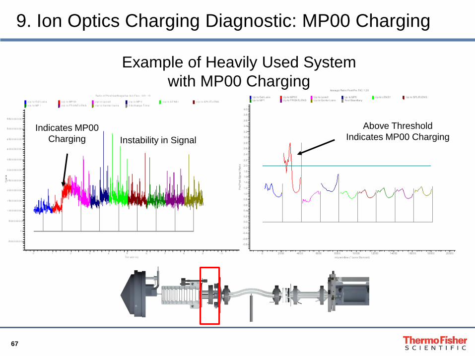
9. Ion Optics Charging Diagnostic: MP00 Charging
Above Threshold
Indicates MP00 Charging Instability in Signal
Indicates MP00
Charging
Example of Heavily Used System
with MP00 Charging
68
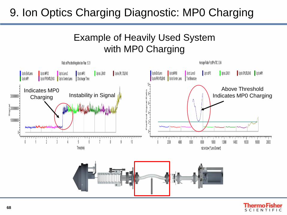
9. Ion Optics Charging Diagnostic: MP0 Charging
Example of Heavily Used System
with MP0 Charging
Above Threshold
Indicates MP0 Charging Instability in Signal Indicates MP0
Charging
69
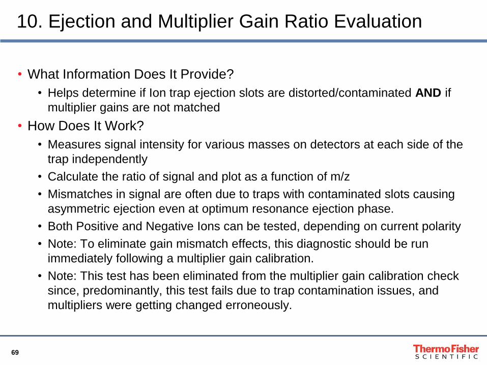
10. Ejection and Multiplier Gain Ratio Evaluation
• What Information Does It Provide?
• Helps determine if Ion trap ejection slots are distorted/contaminated AND if
multiplier gains are not matched
• How Does It Work?
• Measures signal intensity for various masses on detectors at each side of the
trap independently
• Calculate the ratio of signal and plot as a function of m/z
• Mismatches in signal are often due to traps with contaminated slots causing
asymmetric ejection even at optimum resonance ejection phase.
• Both Positive and Negative Ions can be tested, depending on current polarity
• Note: To eliminate gain mismatch effects, this diagnostic should be run
immediately following a multiplier gain calibration.
• Note: This test has been eliminated from the multiplier gain calibration check
since, predominantly, this test fails due to trap contamination issues, and
multipliers were getting changed erroneously.
70
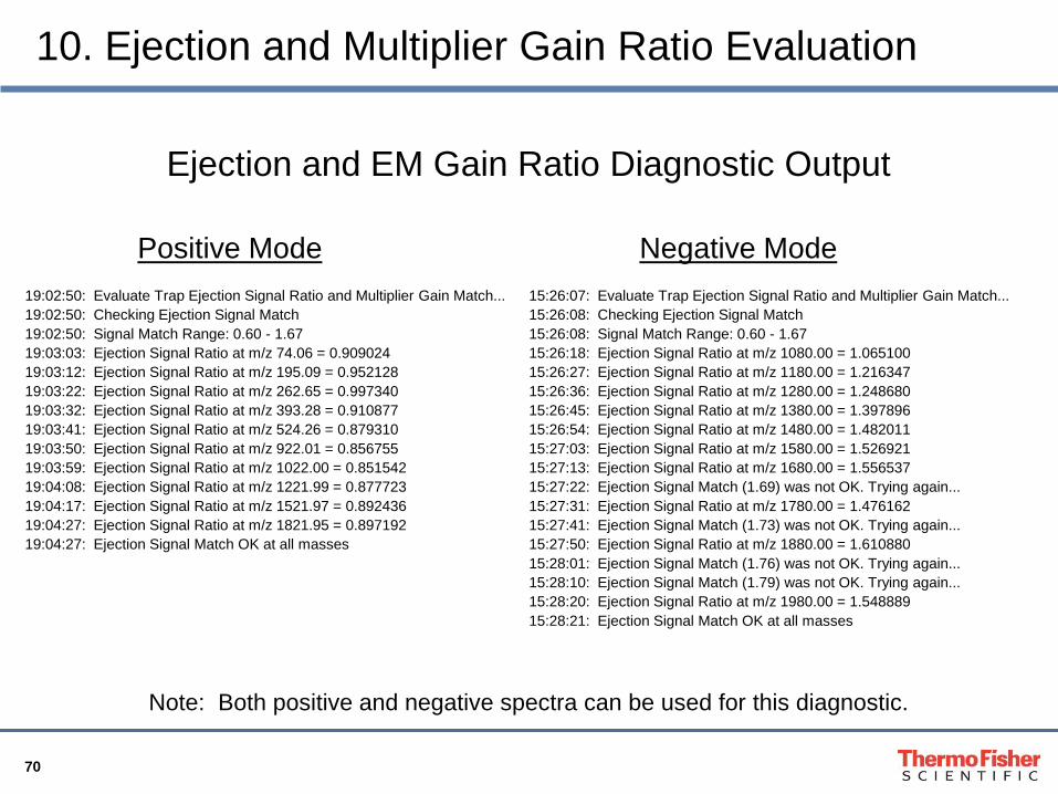
10. Ejection and Multiplier Gain Ratio Evaluation
19:02:50: Evaluate Trap Ejection Signal Ratio and Multiplier Gain Match...
19:02:50: Checking Ejection Signal Match
19:02:50: Signal Match Range: 0.60 - 1.67
19:03:03: Ejection Signal Ratio at m/z 74.06 = 0.909024
19:03:12: Ejection Signal Ratio at m/z 195.09 = 0.952128
19:03:22: Ejection Signal Ratio at m/z 262.65 = 0.997340
19:03:32: Ejection Signal Ratio at m/z 393.28 = 0.910877
19:03:41: Ejection Signal Ratio at m/z 524.26 = 0.879310
19:03:50: Ejection Signal Ratio at m/z 922.01 = 0.856755
19:03:59: Ejection Signal Ratio at m/z 1022.00 = 0.851542
19:04:08: Ejection Signal Ratio at m/z 1221.99 = 0.877723
19:04:17: Ejection Signal Ratio at m/z 1521.97 = 0.892436
19:04:27: Ejection Signal Ratio at m/z 1821.95 = 0.897192
19:04:27: Ejection Signal Match OK at all masses
Note: Both positive and negative spectra can be used for this diagnostic.
15:26:07: Evaluate Trap Ejection Signal Ratio and Multiplier Gain Match...
15:26:08: Checking Ejection Signal Match
15:26:08: Signal Match Range: 0.60 - 1.67
15:26:18: Ejection Signal Ratio at m/z 1080.00 = 1.065100
15:26:27: Ejection Signal Ratio at m/z 1180.00 = 1.216347
15:26:36: Ejection Signal Ratio at m/z 1280.00 = 1.248680
15:26:45: Ejection Signal Ratio at m/z 1380.00 = 1.397896
15:26:54: Ejection Signal Ratio at m/z 1480.00 = 1.482011
15:27:03: Ejection Signal Ratio at m/z 1580.00 = 1.526921
15:27:13: Ejection Signal Ratio at m/z 1680.00 = 1.556537
15:27:22: Ejection Signal Match (1.69) was not OK. Trying again...
15:27:31: Ejection Signal Ratio at m/z 1780.00 = 1.476162
15:27:41: Ejection Signal Match (1.73) was not OK. Trying again...
15:27:50: Ejection Signal Ratio at m/z 1880.00 = 1.610880
15:28:01: Ejection Signal Match (1.76) was not OK. Trying again...
15:28:10: Ejection Signal Match (1.79) was not OK. Trying again...
15:28:20: Ejection Signal Ratio at m/z 1980.00 = 1.548889
15:28:21: Ejection Signal Match OK at all masses
Ejection and EM Gain Ratio Diagnostic Output
Positive Mode Negative Mode

71
10. Ejection and Multiplier Gain Ratio Evaluation
Comparing Signals at Each Detector for m/z 1821.95
2 4 6 8 10 12 14 16 18 20 22 24 26
Scan
Detector 1 Detector 2
-6000000
-5000000
-4000000
-3000000
-2000000
-1000000
0
1000000
2000000
3000000
4000000
5000000
6000000
7000000
8000000
9000000
10000000
11000000
12000000
13000000
TIC
Ejection Signal Ratio vs M/Z
200 400 600 800 1000 1200 1400 1600 1800 2000
M/Z
0.1
0.2
0.3
0.4
0.5
0.6
0.7
0.8
0.9
1.0
1.1
1.2
1.3
1.4
1.5
1.6
1.7
1.8
1.9
2.0
Sig
nal R
atio
Top Graph Bottom Graph
72
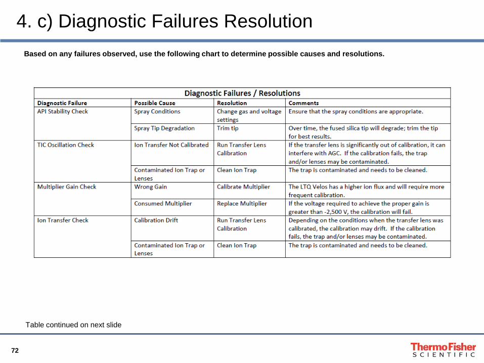
4. c) Diagnostic Failures Resolution
Table continued on next slide
Based on any failures observed, use the following chart to determine possible causes and resolutions.
73
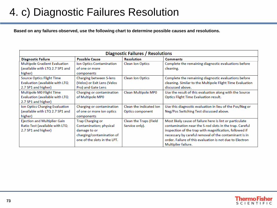
4. c) Diagnostic Failures Resolution
Based on any failures observed, use the following chart to determine possible causes and resolutions.
74
4. c) Diagnostic Failures Resolution
• Based upon the data provided by the diagnostic checks described
above, there are several possible steps which may be necessary to
restore sensitivity, including:
• Restoring the default ion optics tune voltages.
• Calibrating the electron multipliers and/or Transfer Lenses.
• Cleaning the ion optics.
• Contacting your local Field Service Representative for assistance.
• If it is determined that the Ion Optics requires cleaning, the next section
briefly describes Ion Optics Cleaning.
75
Section I Contents
1. Achieving and Maintaining a Stable Spray
2. Calibrating the Velos Pro
3. Tuning the Velos Pro for Optimal Performance
4. Diagnostics and Troubleshooting on the Velos Pro, Orbitrap Velos
Pro, and Orbitrap Elite: Introducing LTQ 2.7 SP1
5. Cleaning the Ion Optics on the Velos Pro or the Velos Pro part of
the Orbitrap Velos Pro and Orbitrap Elite
6. Communicating with Thermo
76
5. Cleaning the Ion Optics
• Before removing the API stack or the top cover, be sure that the
environment around the instrument is as clean and dust free as
possible.
• After the top cover is removed, it is imperative that the open manifold
be covered with a clean sheet of aluminum foil. This will prevent dust
and particles from falling out of the air and getting into the manifold
causing further charging problems.
77
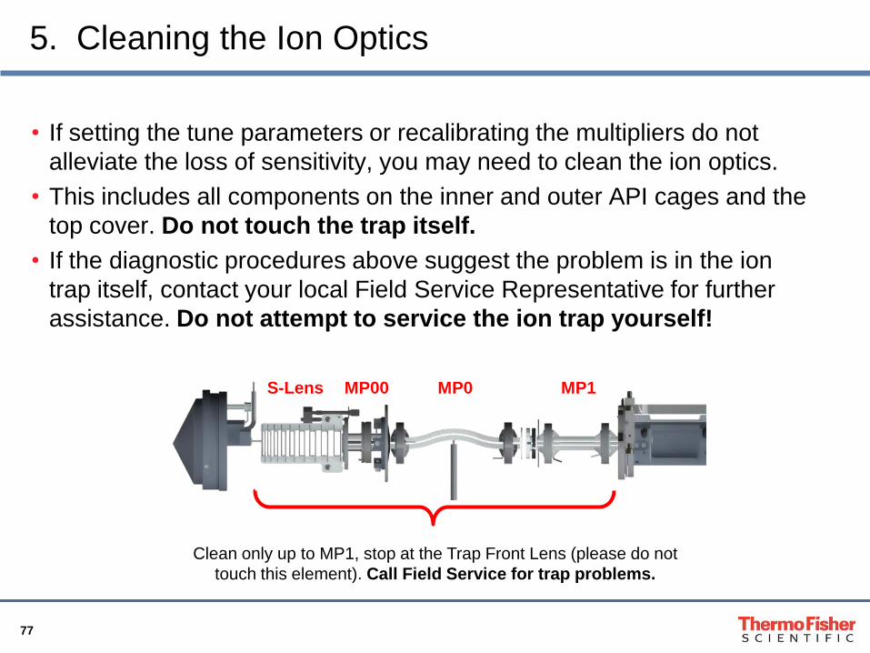
5. Cleaning the Ion Optics
• If setting the tune parameters or recalibrating the multipliers do not
alleviate the loss of sensitivity, you may need to clean the ion optics.
• This includes all components on the inner and outer API cages and the
top cover. Do not touch the trap itself.
• If the diagnostic procedures above suggest the problem is in the ion
trap itself, contact your local Field Service Representative for further
assistance. Do not attempt to service the ion trap yourself!
Clean only up to MP1, stop at the Trap Front Lens (please do not
touch this element). Call Field Service for trap problems.
S-Lens MP00 MP0 MP1
78
5. Cleaning the Ion Optics: Cleaning Kit
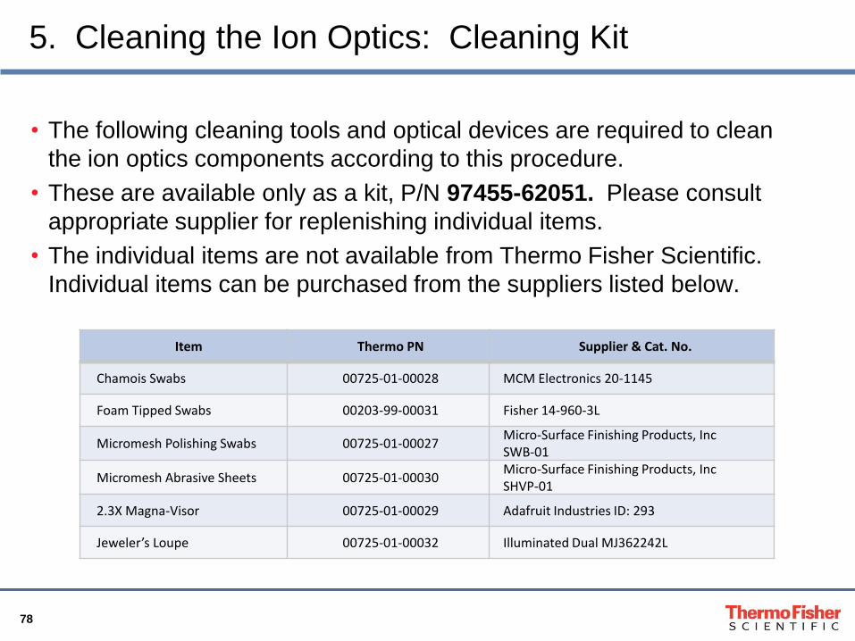
• The following cleaning tools and optical devices are required to clean
the ion optics components according to this procedure.
• These are available only as a kit, P/N 97455-62051. Please consult
appropriate supplier for replenishing individual items.
• The individual items are not available from Thermo Fisher Scientific.
Individual items can be purchased from the suppliers listed below.
Item Thermo PN Supplier & Cat. No.
Chamois Swabs 00725-01-00028 MCM Electronics 20-1145
Foam Tipped Swabs 00203-99-00031 Fisher 14-960-3L
Micromesh Polishing Swabs 00725-01-00027 Micro-Surface Finishing Products, Inc SWB-01
Micromesh Abrasive Sheets 00725-01-00030 Micro-Surface Finishing Products, Inc SHVP-01
2.3X Magna-Visor 00725-01-00029 Adafruit Industries ID: 293
Jeweler’s Loupe 00725-01-00032 Illuminated Dual MJ362242L
79
5. Cleaning the Ion Optics: Removing the Optics
• See the Videos entitled, “Top Cover disassembly, Component Cleaning
and reassembly”, and “Accessing the S-lens, Exit Lens, and MP00 for
Cleaning”, available at http://planetorbitrap.com
• Be sure not to introduce any scratches or surface abrasions while
handling the optics components. Even small scratches can affect
performance if they are near enough to the ion flight path. Avoid using
tools, such as pliers, that may scratch these components.
80
5. Cleaning the Ion Optics: S-Lens
• Carefully inspect the S-Lens with magnification for any lint, particulates, and/or sample
buildup or coatings. After use, there may be some discoloration on some of the lens
elements; this is normal and different from sample build up or coatings. This
discoloration, sometimes called „ion burn‟, has not shown to have any effect on
instrument performance.
• If sonication is available, sonicate the S-Lens in either 50:50 methanol:water or a 1%
solution of Liquinox in water for 10 – 15 minutes.
• If sonication is not available, use a chamois tip swab to clean the S-Lens with a 1%
solution of Liquinox in water. Use a 6000 grit Micromesh swab to clean the areas in the
lens stack that are not accessible to the chamois tip swab.
• Rinse the S-Lens thoroughly with water.
• Rinse the S-Lens with methanol.
• Dry the S-Lens with a stream of nitrogen gas until it is dry. The source of the nitrogen
gas must be oil free.
• Inspect the S-Lens with magnification for any lint or particulates that may have been
introduced by this cleaning procedure. Pay special attention to the orifices and
confirm that no lint or particulate is present in the bore of the orifices. Use
tweezers or similar tools to remove the lint or particulates.
81
5. Cleaning the Ion Optics: Exit Lens
• Carefully inspect the Exit Lens with magnification for any lint, particulates, and/or sample
buildup or coatings. After use, there may be some discoloration the lens surface; this is
normal and different from sample build up or coatings. This discoloration, sometimes
called „ion burn‟, has not shown any effect on instrument performance.
• If sonication is available, sonicate the Exit Lens in either 50:50 methanol:water or a 1%
solution of Liquinox in water for 10 – 15 minutes.
• If sonication is not available, use a soft toothbrush to clean the Exit Lens with a 1%
solution of Liquinox in water.
• Use rolled 6000 grit Micromesh to clean the bore the Exit Lens orifice.
• Rinse the Exit Lens thoroughly with water.
• Rinse the Exit Lens with methanol.
• Dry the Exit Lens with a stream of nitrogen gas until it is dry. The source of the nitrogen
gas must be oil free.
• Inspect the Exit Lens with magnification for any lint or particulates that may have been
introduced by this cleaning procedure. Pay special attention to the orifice and
confirm that no lint or particulate is present in the bore of the orifice. Use tweezers
or similar tools to remove the lint or particulates.
82
5. Cleaning the Ion Optics: Inter Multipole Lenses
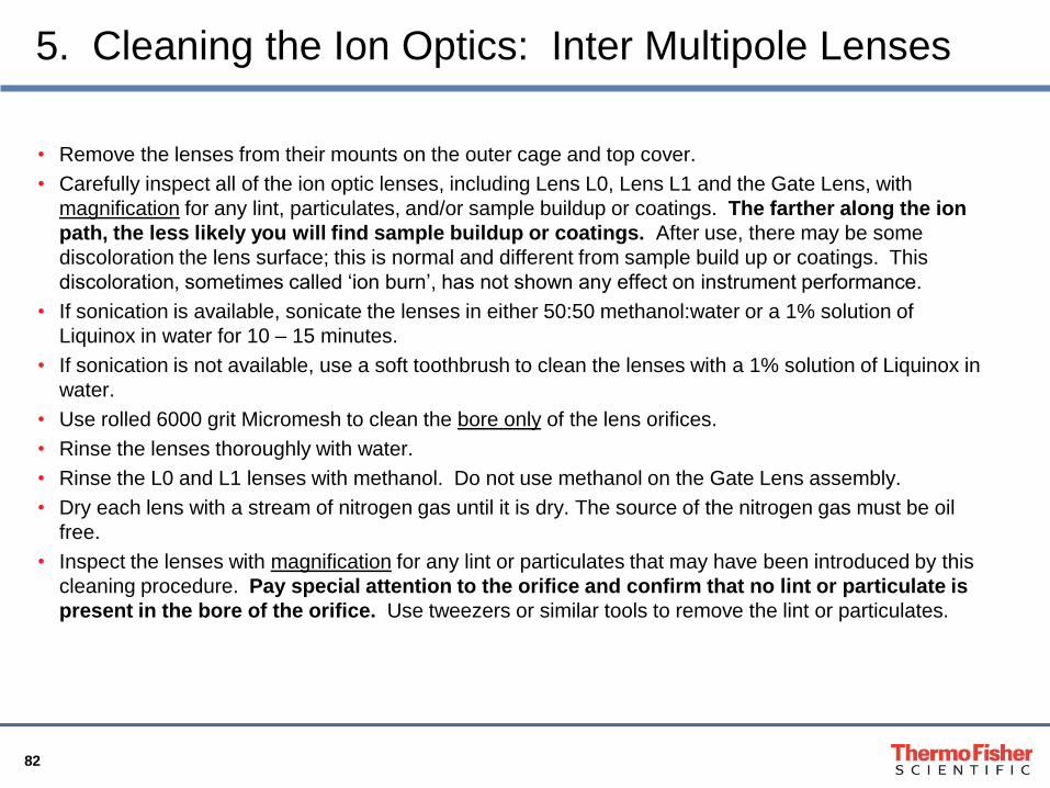
• Remove the lenses from their mounts on the outer cage and top cover.
• Carefully inspect all of the ion optic lenses, including Lens L0, Lens L1 and the Gate Lens, with
magnification for any lint, particulates, and/or sample buildup or coatings. The farther along the ion
path, the less likely you will find sample buildup or coatings. After use, there may be some
discoloration the lens surface; this is normal and different from sample build up or coatings. This
discoloration, sometimes called „ion burn‟, has not shown any effect on instrument performance.
• If sonication is available, sonicate the lenses in either 50:50 methanol:water or a 1% solution of
Liquinox in water for 10 – 15 minutes.
• If sonication is not available, use a soft toothbrush to clean the lenses with a 1% solution of Liquinox in
water.
• Use rolled 6000 grit Micromesh to clean the bore only of the lens orifices.
• Rinse the lenses thoroughly with water.
• Rinse the L0 and L1 lenses with methanol. Do not use methanol on the Gate Lens assembly.
• Dry each lens with a stream of nitrogen gas until it is dry. The source of the nitrogen gas must be oil
free.
• Inspect the lenses with magnification for any lint or particulates that may have been introduced by this
cleaning procedure. Pay special attention to the orifice and confirm that no lint or particulate is
present in the bore of the orifice. Use tweezers or similar tools to remove the lint or particulates.
83
5. Cleaning the Ion Optics: Quadrupole Ion Guides
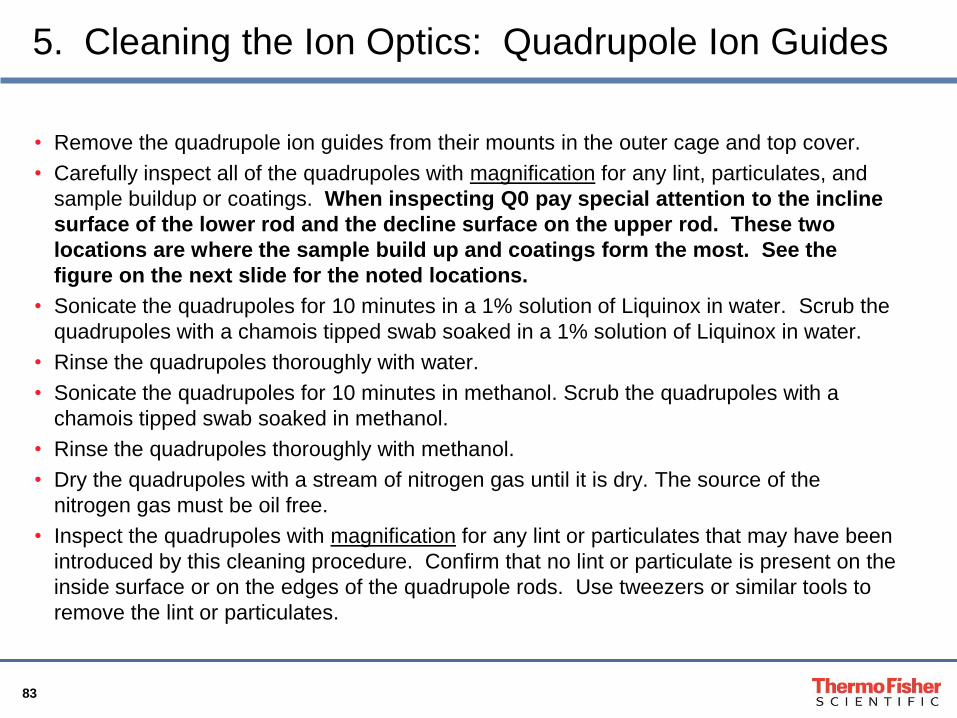
• Remove the quadrupole ion guides from their mounts in the outer cage and top cover.
• Carefully inspect all of the quadrupoles with magnification for any lint, particulates, and
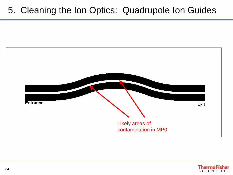
sample buildup or coatings. When inspecting Q0 pay special attention to the incline
surface of the lower rod and the decline surface on the upper rod. These two
locations are where the sample build up and coatings form the most. See the
figure on the next slide for the noted locations.
• Sonicate the quadrupoles for 10 minutes in a 1% solution of Liquinox in water. Scrub the
quadrupoles with a chamois tipped swab soaked in a 1% solution of Liquinox in water.
• Rinse the quadrupoles thoroughly with water.
• Sonicate the quadrupoles for 10 minutes in methanol. Scrub the quadrupoles with a
chamois tipped swab soaked in methanol.
• Rinse the quadrupoles thoroughly with methanol.
• Dry the quadrupoles with a stream of nitrogen gas until it is dry. The source of the
nitrogen gas must be oil free.
• Inspect the quadrupoles with magnification for any lint or particulates that may have been
introduced by this cleaning procedure. Confirm that no lint or particulate is present on the
inside surface or on the edges of the quadrupole rods. Use tweezers or similar tools to
remove the lint or particulates.
84
5. Cleaning the Ion Optics: Quadrupole Ion Guides
Likely areas of
contamination in MP0
85
Section I Contents
1. Achieving and Maintaining a Stable Spray
2. Calibrating the Velos Pro
3. Tuning the Velos Pro for Optimal Performance
4. Diagnostics and Troubleshooting on the Velos Pro, Orbitrap Velos
Pro, and Orbitrap Elite: Introducing LTQ 2.7 SP1
5. Cleaning the Ion Optics on the Velos Pro or the Velos Pro part of the
Orbitrap Velos Pro and Orbitrap Elite
6. Communicating with Thermo
86
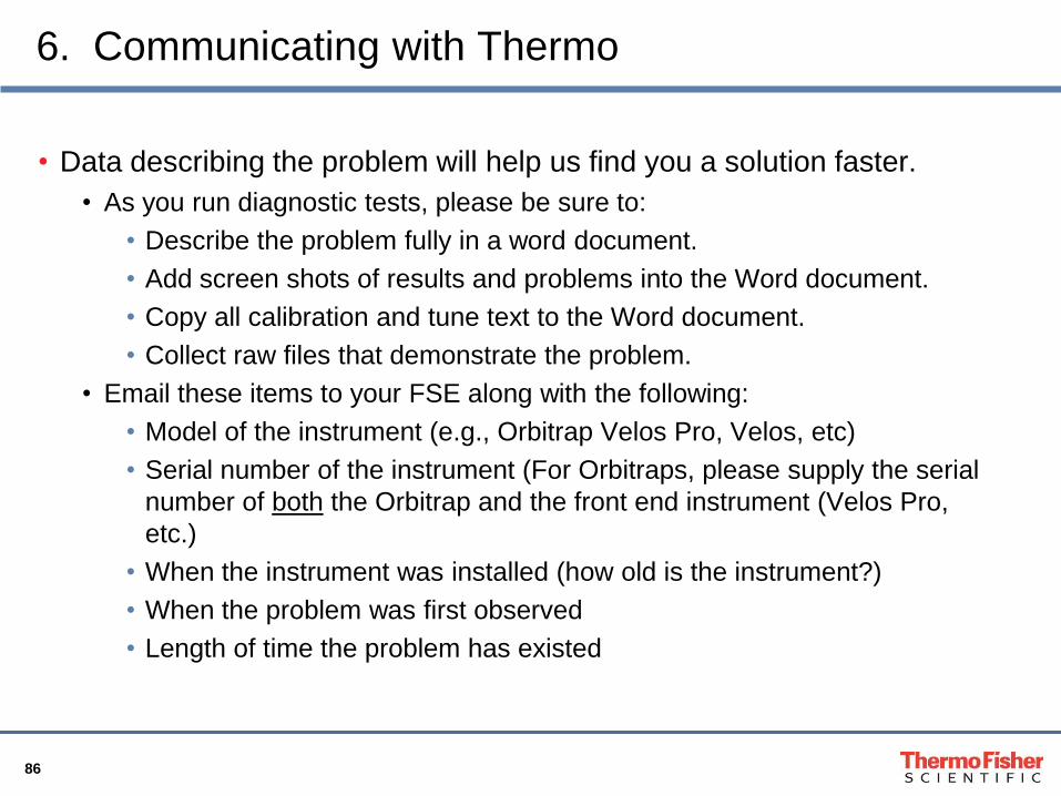
6. Communicating with Thermo
• Data describing the problem will help us find you a solution faster.
• As you run diagnostic tests, please be sure to:
• Describe the problem fully in a word document.
• Add screen shots of results and problems into the Word document.
• Copy all calibration and tune text to the Word document.
• Collect raw files that demonstrate the problem.
• Email these items to your FSE along with the following:
• Model of the instrument (e.g., Orbitrap Velos Pro, Velos, etc)
• Serial number of the instrument (For Orbitraps, please supply the serial
number of both the Orbitrap and the front end instrument (Velos Pro,
etc.)
• When the instrument was installed (how old is the instrument?)
• When the problem was first observed
• Length of time the problem has existed
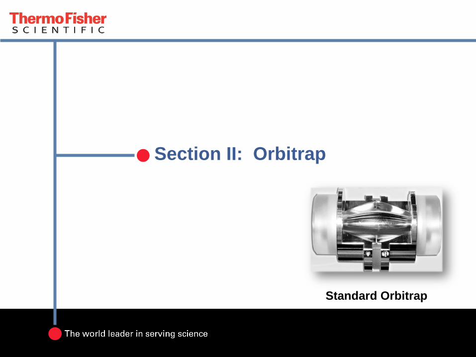
Section II: Orbitrap
Standard Orbitrap
88
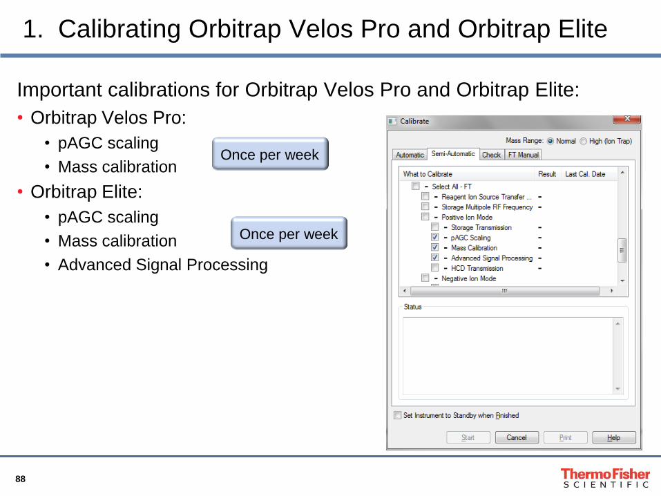
1. Calibrating Orbitrap Velos Pro and Orbitrap Elite
Important calibrations for Orbitrap Velos Pro and Orbitrap Elite:
• Orbitrap Velos Pro:
• pAGC scaling
• Mass calibration
• Orbitrap Elite:
• pAGC scaling
• Mass calibration
• Advanced Signal Processing
Once per week
Once per week
89
1.a) Predictive AGC (pAGC) Scaling Calibration
4.0 4.2 4.4 4.6 4.8 5.0 5.2 5.4 5.6 5.8 6.0 6.2 6.4
lg(target)
5
10
15
20
25
30
35
40
45
50
55
60
65
70
75
80
85
90
95
100
105
110
115
120
pre
dic
tive
AG
C s
ca
le fa
cto
r
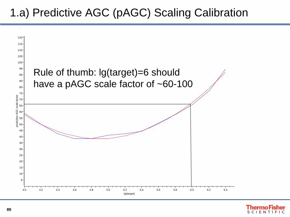
Rule of thumb: lg(target)=6 should
have a pAGC scale factor of ~60-100
90
1.a) Predictive AGC (pAGC) Scaling Calibration
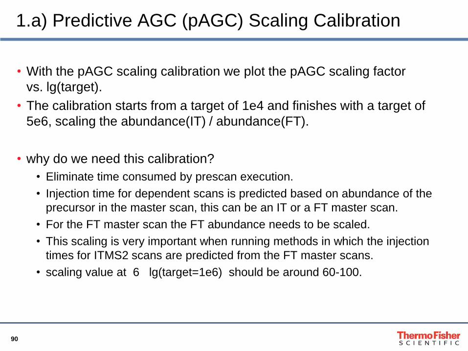
• With the pAGC scaling calibration we plot the pAGC scaling factor
vs. lg(target).
• The calibration starts from a target of 1e4 and finishes with a target of
5e6, scaling the abundance(IT) / abundance(FT).
• why do we need this calibration?
• Eliminate time consumed by prescan execution.
• Injection time for dependent scans is predicted based on abundance of the
precursor in the master scan, this can be an IT or a FT master scan.
• For the FT master scan the FT abundance needs to be scaled.
• This scaling is very important when running methods in which the injection
times for ITMS2 scans are predicted from the FT master scans.
• scaling value at 6 lg(target=1e6) should be around 60-100.
91
1.b) Tips to Check Mass Accuracy
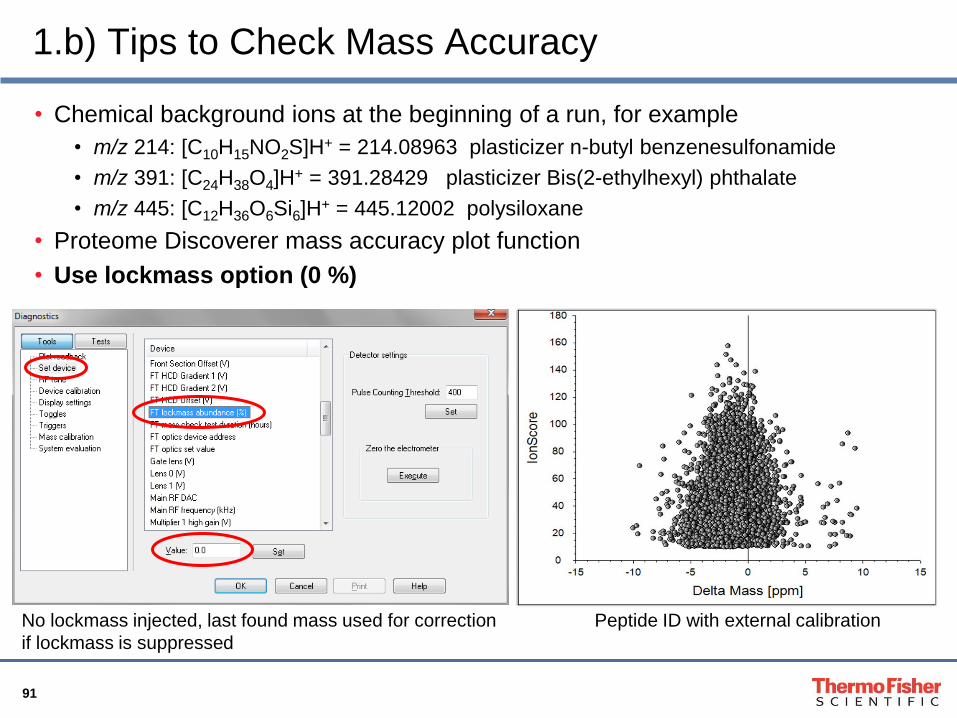
• Chemical background ions at the beginning of a run, for example
• m/z 214: [C10H15NO2S]H+ = 214.08963 plasticizer n-butyl benzenesulfonamide
• m/z 391: [C24H38O4]H+ = 391.28429 plasticizer Bis(2-ethylhexyl) phthalate
• m/z 445: [C12H36O6Si6]H+ = 445.12002 polysiloxane
• Proteome Discoverer mass accuracy plot function
• Use lockmass option (0 %)
No lockmass injected, last found mass used for correction
if lockmass is suppressed
Peptide ID with external calibration
92
1.c) Lock Mass Abundance 0%
• What happens when the lock mass abundance is set to 0%: If the lock
mass is not found in one scan, the system applies the correction from a
previous scan where the LM has been found.
For example, at the beginning of a nanoLC run background ions such as m/z
445: [C12H36O6Si6]H+ = 445.12002 polysiloxane are present and can be used as
lock mass.
• When high abundant peptides are eluting, the chance to lose your lock
mass in the FTMS spectrum is high. In such a case, when the lock
mass isn‟t found, the system will use the correction from a previous
scan where the lock mass was present and will keep this correction
until the lock mass is present again in the FTMS spectrum.
• HCD scans and a LM abundance set to „0%‟, the LM correction is done
based on the LM found in the full Orbi scan.

93
1.c) Lock Mass Abundance 0%
WHY?
• Possible problems that do occur when using lock mass abundance >0%.
• A LM > 0% can result in a reduced scan rate due to the accumulation of
the Lockmass ion.
• Lower Lockmass abundance than expected (from your selected
abundance e.g.5%) may result from different ion source and/or LC
characteristics.
• A Lockmass with lower abundance will have lower signal/noise, leading
to a wider spread of the mass accuracy (Lockmass has more jitter).
• Furthermore, if the Lockmass is lower, there may be occurrences where
the Lockmass is not found leading to mass accuracy deviations.
Recommendation for best mass accuracy:
Use lockmass option 0 %
94
Phone numbers and emails for assistance
• Unity Lab Services: http://www.unitylabservices.com/contact.php
• To contact Technical Support
• Phone 800-532-4752
• FAX 561-688-8736
• E-mail us. [email protected]
• Downloads www.planetorbitrap.com
• To contact Customer Service for ordering information
• Phone 800-532-4752
• FAX 561-688-8731
• E-mail [email protected]
• Web www.thermo.com/ms
• To get local contact information for sales or service
• www.thermoscientific.com/wps/portal/ts/contactus
• To copy manuals from the Internet
• Go to mssupport.thermo.com (agree to Terms and Conditions, then click
Customer Manuals in the left margin of the window)