Int J Adv Manuf Technol (2018) 95:1421–1436https://doi.org/10.1007/s00170-017-1266-1

ORIGINAL ARTICLE

Achievable tolerances in robotic feature machiningoperations using a low-cost hexapod

J. D. Barnfather1 ·M. J. Goodfellow2 ·T. Abram1

Received: 8 June 2017 / Accepted: 26 October 2017 / Published online: 10 November 2017© The Author(s) 2017. This article is an open access publication

Abstract Portable robotic machine tools potentially allowfeature machining processes to be brought to large parts invarious industries, creating an opportunity for capital expen-diture and operating cost reduction. However, robots lackthe machining capability of conventional equipment, whichultimately results in dimensional errors in parts. This workshowcases a low-cost hexapod-based robotic machine tooland presents experimental research conducted to investigatehow the widely researched robotic machining challenges,e.g. structural dynamics and kinematics, translate to achiev-able tolerance ranges in real-world production to high-light currently feasible applications and provide a contextfor considering technology improvements. Machining trialsassess the total dimensional errors in the final part over mul-tiple geometries. A key finding is error variation which isin the sub-millimetre range, although, in some cases, uppertolerance limits < 100 μm are achieved. Practical chal-lenges are also noted. Most significantly, it is demonstratedthat dimensional machining error is mainly systematic innature and therefore that the total error can be dramati-cally reduced with in situ measurement and compensation.Potential is therefore found to achieve a flexible, high-performance robotic machining capability despite complexand diverse underlying scientific challenges. Overall, the

� J. D. Barnfatherjoshbarnfather@gmail.com

1 The Department of Mechanical, Aerospace and CivilEngineering, The University of Manchester, PariserBuilding, Sackville Street, Manchester M13 9PL, UK

2 Civil Nuclear, Rolls-Royce Plc., PO Box 2000, Raynesway,Derby, DE23 7XX, UK

work presented highlights achievable tolerances in low-cost robotic machining and opportunities for improvement,also providing a practical benchmark useful for processselection.

Keywords Machining · Robot · Tolerance · Hexapod ·Performance · Error

1 Introduction

Robots are attracting interest in the nuclear, oil and gasand aerospace industries for machining relatively small fea-tures on large parts without reliance on conventional, largemachine tools. This potentially reduces capital expenditureand operational costs and avoids heavy lifting by bringingthe machining process to the part rather than moving largecomponents around manufacturing facilities, which causesa health and safety concern. As noted by Wang et al. in[1], this is possible due to the availability of high-accuracylarge-volume metrology equipment, such as laser track-ers and indoor GPS systems, for robot positioning aroundlarge components, which potentially leads to high accu-racy of feature positions. A brief application case study canbe found in [2], which is particularly relevant to nuclearpower plant components with feature tolerances of 100 μmto 5 mm for weld prep, weld dressing, instrumentationpenetration, nozzle and manway geometry.

High-tolerance robotic machining of metals is a devel-oping technology, competing with conventional machinetools that can achieve tolerances of single microns [3].Robotic machining has a range of technical barriers asso-ciated with it, which must be overcome before economicbenefits can be exploited. This investigation provides a valu-able contribution to the development of robotic machining

1422 Int J Adv Manuf Technol (2018) 95:1421–1436

techniques by characterising known technical challenges interms of the overall achievable tolerances. Achievable tol-erance characterisation is novel because it encompasses allerror-contributing phenomena, using low-cost equipment,rather than a single source as is typical in the literature.

For example, kinematic modelling is widely researchedas a key issue in accurate robot manipulation becausethis relates the programmed end effector positions to jointrotations and actuator extensions. Robot kinematics are dis-cussed by Weill et al., where dimensional errors in linksand joints are noted to cause assembly misalignments andtherefore differences between the nominal kinematic model,used in the controller, and the real world [4]. In uncon-ventional parallel robot structures, which have a complexconfiguration of actuators and joints, such differences aredue to difficulties in modelling the non-linear mappingbetween actuator and machining coordinate spaces [5]. Thisis problematic because parallel kinematic hexapod robotsare desirable for machining due to their stiffness benefits[6–11].

Fassi and Wiens support kinematic modelling challengesbut note that parallel robotic configurations have a non-cumulative error stack up in links and joints, which the-oretically provides improved accuracy compared to serial-arm alternatives [12]. Agheli and Nategh discuss kinematicmodel calibration using a hexapod robot and find thatoptimum results are achieved when models are based onmaximum observable robot error measurements, which areat the limits of the working envelope in this case [9]. Thispotentially introduces challenges in identifying the high-est error levels in other robot configurations because Halajand Kurekova conclude that positional errors vary over theworking envelope [13].

As well as kinematic modelling issues, Fassi and Wienshighlight concerns over dynamic structural rigidity issuesand their influence on part quality in robotic machining[12]. Zhang et al. note that the stiffness for a typical indus-trial robot is around 1 N/μm, whereas a typical machinetool has stiffness greater than 50 N/μm and also expressesaccuracy concerns for robotic machining due to machiningforces and imperfect kinematic models [14]. This is sup-ported by Doukas et al. who present experimental results ondeflection behaviour [15]. Pandremenos et al. back up rigid-ity concerns further with experimental results highlightingaccuracy and chatter issues [16]. In addition, joint stiffnessis specifically discussed as an influence on part quality byDumas et al., although data is difficult to obtain from robotmanufacturers and user evaluation is recommended [17].

Work done by Sornmo et al. attempts to counteract rigid-ity problems with adaptive force control in robot machining,discussing how part inaccuracy is caused by excessive pro-cess forces that result in deviations from programmed paths[18]. Matsuoka et al. also highlight the importance of

this issue by testing different machining strategies for bestforce management [19]. Lehmann et al. combine adaptiveforce control, strategy optimisation and off-line force com-pensation techniques for part accuracy improvement [20].Olofsson et al. also consider machining force compensationby using a piezo-actuated micro-manipulator to compensatefor tool deflection [21].

Further robotic machining literature is available thatbacks up kinematic and structural dynamic concerns. Forexample, the research of Abele et al. focuses on both thekinematic and stiffness modelling of a serial-arm roboticmachine tool, highlighting dynamic differences from con-ventional machine tools and tool displacement problems[22]. Also, Bouzgarrou et al. and Li et al. follow a similartheme in the context of a parallel kinematic design robot [23,24]. The influence of cutting force, structural rigidity andfull kinematics compensation on robotic machining accu-racy is, again, noted by Wu et al. and Pessi et al. [25–27].Pan and Zhang expand on the issues mentioned by consid-ering the impact of rigidity on low material removal rateand chatter, and implement a real-time compensation algo-rithm based on stiffness modelling to counteract this [28].Work by Pan et al. relates cutting force and structural rigid-ity models to chatter issues in robotic machining, presentingstability criteria and highlighting the difference betweenconventional machine tool characteristics [29].

Conventional machine tool issues, including gear backlash and wear [30], are exaggerated in robotic machiningdue to structural differences [31]. Gong et al. also suggestthat non-geometric robot errors should also be offset byaccounting for thermal variations and joint flexibility underload [32]. Thermal concerns are supported by Kamrani etal. [33]. In research published by Antunes Simoes et al., therelationship between optimised process variable selectionand the surface quality and dimensional error is highlighted,although this is in the context of robotic machining of plas-ter parts [34]. Olabi et al. highlights that trajectory planningis a key non-geometric contributor to path error [35], backedup by Zargarbashi et al. [36, 37]. This issue and robot feedrate accuracy, as assessed by Young and Pickin [38], arekey research areas for improving machined surface quality.Chen and Dong show that robot repeatability decreases withreach and supports concerns over chatter, path planning,calibration and low material removal rates [39].

Overall, the robotic machining literature available high-lights a complex and diverse range of research issues thatresult in poor part quality. This literature is well justi-fied for tackling other challenges but it does not give athorough insight into the combined overall impact thatrobotic machining downfalls have on achievable tolerancesin real-world production. Here, a novel low-cost roboticmachine tool is proposed using the Fanuc F200iB hexa-pod and achievable tolerance ranges are investigated for

Int J Adv Manuf Technol (2018) 95:1421–1436 1423

various geometries with machining trials. More specifically,the experimental investigation presented builds on the workof Tunc et al. [40–42] who assess dynamic stiffness varianceof the same Fanuc F200iB hexapod robot over its workingvolume and the implications for machining accuracy.

The contribution made is the provision of practical dataand analysis for use by manufacturers to improve low-costindustrial robot-based machine tools and to determine appli-cations for current implementation. This is needed becausethe literature associated with specific issues contributing todimensional errors does not completely provide this high-level perspective alone. The intended impact is therefore toencourage development by highlighting applications whererobotic machining can be feasibly adopted in addition tothe scale of challenges. The results presented also serveas a benchmark for comparing technology improvementsagainst, which is necessary to push robotic machining tech-nology further. It therefore allows advances associated withindividual error contributors to be considered in the contextof a key high-level problem.

An account of work done is presented beginning withdefinitions of terms and the analysis procedure used inSection 2. An overview of the equipment used, details ofthe experimental set-up and methodology are then given inSections 3 and 4, respectively. Finally, data is analysed todetermine machining performance indices in Section 5 andfindings are summarised in Section 6.

2 Definitions and theory

This section describes the definitions and theory associatedwith the experiments in Section 2.1 and analysing the dataacquired in Section 2.2.

2.1 Machining parameters

Spindle speed, N in RPM, for maximum stable machin-ing efficiency is determined through modal analysis, asexplained in the Section 3. N is related to feed rate, vf inmillimetres per minute, using Eq. 1, where fz is the chipload per tooth in millimetres, taken from tool manufacturerrecommendations, and zc is the number of tool teeth.

vf = fz × N × zc (1)

Material removal rate, Q in cubic centimetres per minute,is given by Eq. 2, where ap is the axial depth of cut in mil-limetres and ae is the radial depth of cut in millimetre, alsodetermined through modal analysis.

Q = ap × ae × vf

1000(2)

The tool life criterion used to approximate useful toolcutting time, T in minutes, before degradation occurs tothe degree that the tool can no longer cut required dimen-sions, is defined as a uniform flank wear land, VB, of0.3 mm averaged over all teeth in dry cutting conditions.This criterion is recommended by ISO 8688-2 [43] andis estimated according to Taylor method [44]. Taylor toollife estimation is widely utilised and recommended in var-ious works [45–50]. Wang et al. support the idea that toollife can be estimated in robotic machining when stablecutting parameters are established [51], i.e. with modalanalysis. Tool life estimates are qualitatively verified bythe operator with regular visual tool inspection in betweenoperations and by listening for changes in machiningnoise.

T is given by the following equations [48]. n is Taylortool life exponent and is computed from reference tool lives,TRA and TRB, at the extreme upper and lower ranges for agiven tool, which correspond to the reference cutting speedsvcRA and vcRB in metres per minute. These reference val-ues are provided for each tool by their manufacturer in drycutting conditions. C is the Taylor constant and computedusing n and vcRA. Finally, T for the real cutting conditionsused in experiments is estimated using Eq. 5, where vc is thecutting speed dependent on the cutting diameter at ap, Dcap,determined through modal analysis of the specific robot andtool set-up.

n = ln vcRB − ln vcRA

ln TRA − ln TRB(3)

C = vcRA × T nRA (4)

T =(

C

vc

)1/n

(5)

vc = Dcap × π × N

1000(6)

2.2 Experimental data analysis

Experimental data analysis theory is based on previous workdone to develop a robotic machine tool performance evalua-tion methodology based on standards published on roboticsand machining independently [2]. Interested readers aredirected to this paper for detailed information on the theoryused.

In machining trials, the upper machine performanceindex, PmkU, is estimated with a confidence interval tojudge the ability of the process to achieve upper toleranceslimits according to methods described in [2]. A prerequi-site to index computation is to plot errors between nom-inal and measured dimensions with a run chart to assess

1424 Int J Adv Manuf Technol (2018) 95:1421–1436

statistical control, where instability is indicated by steppedvariation. Non-normally distributed data may occur due tooutliers, process variables shifts, biases and process limitsor because it has a different distribution. To determine thespecific estimation method for PmkU, distribution class isassessed to check for normality, which is indicated graphi-cally using histograms with fitted ideal normal distributioncurves and using normality tests when sample size is ≥ 30,as recommended by Razali et al. [52].

The Anderson-Darling normality test is chosen becauseit achieved a consistently high statistical power in theRazali et al. study in comparison to alternatives. Normal-ity tests reject the null hypothesis that the data is normallydistributed if the estimated probability, P value, of com-puting the test statistic, A2, for a normal distribution is≤ 0.05. The P value is determined from critical values ofA2 [53, 54].

In cases where a normal distribution is not observed,data is transformed using the Box-Cox method [55], as rec-ommended by Hosseinifard et al. [56]. To do this, eachindividual value from the dataset, yi , is raised to the powerof λ, which is found by searching for the optimum valuebetween - 5 and 5 to achieve normality according to A2,excluding zero where the natural logarithm of the dataset istaken. If transformation is unsuccessful, alternate computa-tion methods are used as specified in the key reference givenabove [2].

y(λ)i =

{yλi −1λ

; λ �= 0log yi; λ = 0

(7)

In analysis of variance (ANOVA) tables plotted ongraphs, the ‘Groups’ row contains analysis statistics fortesting variation between data groups and the ‘Error’ rowcontains analysis statistics for testing variation within datagroups. For both rows, the sum of squares of the observa-tions is given by SS, the degrees of freedom is given bydf and the ratio between SS and df is given by the meansquared error, MS. The ratio between MS for each variationsource is given by the F-statistic, F . The probability of F

actually being higher is given by Prob > F and indicatesa significant difference between data groups when it has avalue ≤ 0.05.

3 Equipment and set-up

The following sub-sections describe the equipment and set-up procedures used to conduct experiments. This beginswith a description of the robotic machine tool proposed andtested in Section 3.1 and then its alignment and position-ing procedures in Section 3.2. Test geometry, tooling andprogramming details are given in Sections 3.3–3.5.

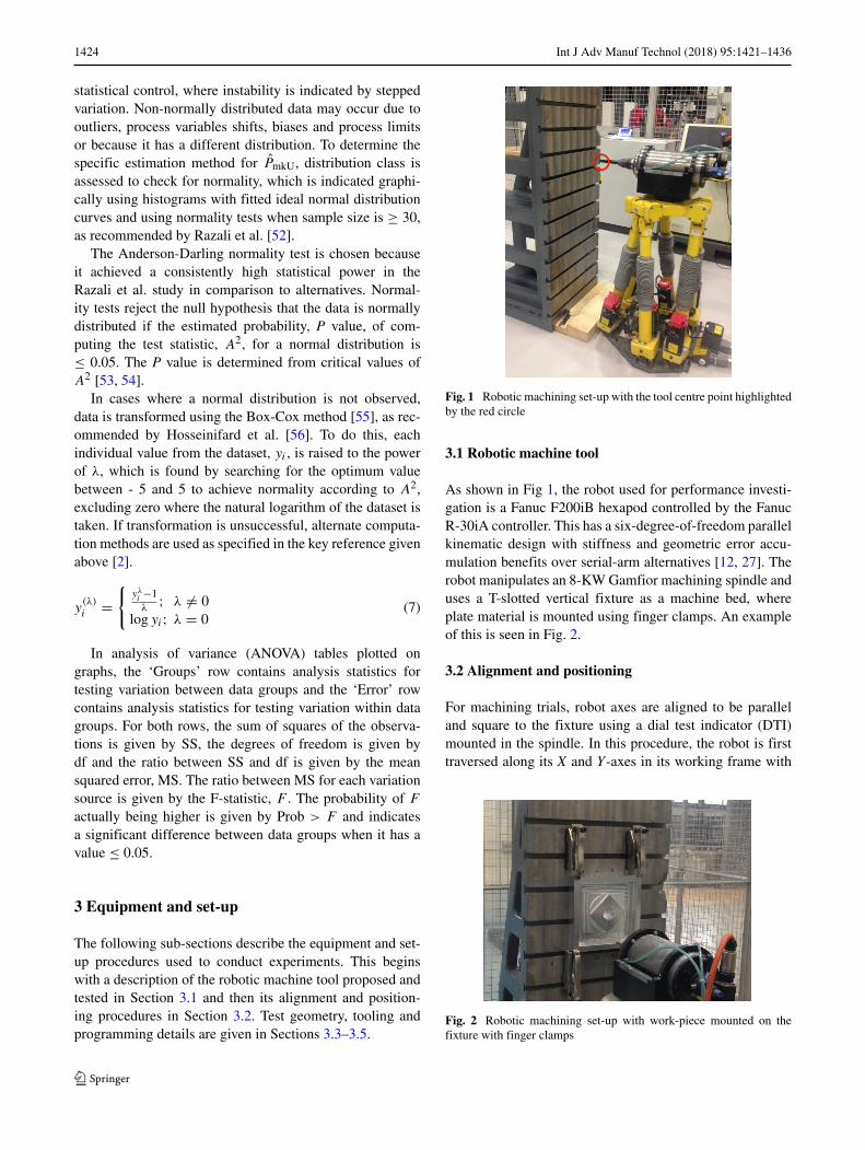
Fig. 1 Robotic machining set-up with the tool centre point highlightedby the red circle

3.1 Robotic machine tool

As shown in Fig 1, the robot used for performance investi-gation is a Fanuc F200iB hexapod controlled by the FanucR-30iA controller. This has a six-degree-of-freedom parallelkinematic design with stiffness and geometric error accu-mulation benefits over serial-arm alternatives [12, 27]. Therobot manipulates an 8-KW Gamfior machining spindle anduses a T-slotted vertical fixture as a machine bed, whereplate material is mounted using finger clamps. An exampleof this is seen in Fig. 2.

3.2 Alignment and positioning

For machining trials, robot axes are aligned to be paralleland square to the fixture using a dial test indicator (DTI)mounted in the spindle. In this procedure, the robot is firsttraversed along its X and Y-axes in its working frame with

Fig. 2 Robotic machining set-up with work-piece mounted on thefixture with finger clamps

Int J Adv Manuf Technol (2018) 95:1421–1436 1425

the indicator pressed against the fixture. Non-parallelism isdetected when values on the DTI are not constant duringthese motions. Corrections are made by manually adjustingthe working frame rotations to achieve a constant indicatorreading during traverse motions.

Squareness is corrected by manually rotating the DTI inthe spindle, with it offset from the centre of rotation andpressed on the fixture, to trace out a circular path. Thespindle is shown not to be square to the fixture if values indi-cated are not constant. Squareness corrections are made bymanually adjusting the tool frame rotations, which relatesthe robot world coordinate system to the end effector. Theoverall alignment quality is limited by the flatness of thefixture and the uncertainty of the DTI.

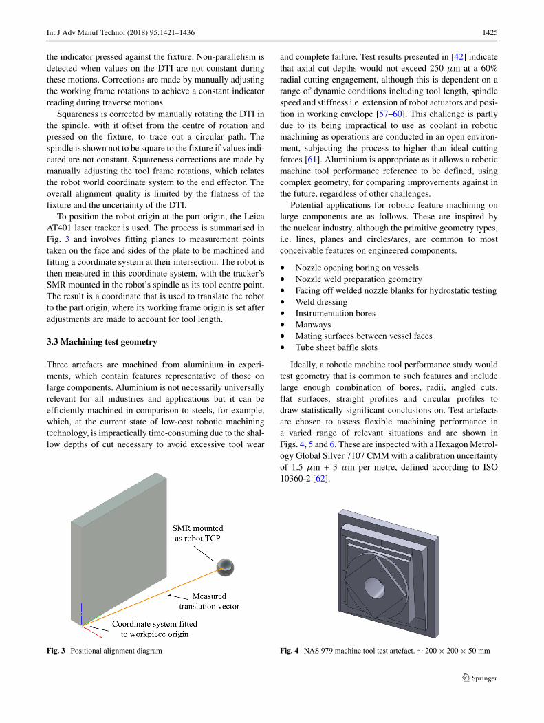
To position the robot origin at the part origin, the LeicaAT401 laser tracker is used. The process is summarised inFig. 3 and involves fitting planes to measurement pointstaken on the face and sides of the plate to be machined andfitting a coordinate system at their intersection. The robot isthen measured in this coordinate system, with the tracker’sSMR mounted in the robot’s spindle as its tool centre point.The result is a coordinate that is used to translate the robotto the part origin, where its working frame origin is set afteradjustments are made to account for tool length.

3.3 Machining test geometry

Three artefacts are machined from aluminium in experi-ments, which contain features representative of those onlarge components. Aluminium is not necessarily universallyrelevant for all industries and applications but it can beefficiently machined in comparison to steels, for example,which, at the current state of low-cost robotic machiningtechnology, is impractically time-consuming due to the shal-low depths of cut necessary to avoid excessive tool wear

Fig. 3 Positional alignment diagram

and complete failure. Test results presented in [42] indicatethat axial cut depths would not exceed 250 μm at a 60%radial cutting engagement, although this is dependent on arange of dynamic conditions including tool length, spindlespeed and stiffness i.e. extension of robot actuators and posi-tion in working envelope [57–60]. This challenge is partlydue to its being impractical to use as coolant in roboticmachining as operations are conducted in an open environ-ment, subjecting the process to higher than ideal cuttingforces [61]. Aluminium is appropriate as it allows a roboticmachine tool performance reference to be defined, usingcomplex geometry, for comparing improvements against inthe future, regardless of other challenges.

Potential applications for robotic feature machining onlarge components are as follows. These are inspired bythe nuclear industry, although the primitive geometry types,i.e. lines, planes and circles/arcs, are common to mostconceivable features on engineered components.

• Nozzle opening boring on vessels• Nozzle weld preparation geometry• Facing off welded nozzle blanks for hydrostatic testing• Weld dressing• Instrumentation bores• Manways• Mating surfaces between vessel faces• Tube sheet baffle slots

Ideally, a robotic machine tool performance study wouldtest geometry that is common to such features and includelarge enough combination of bores, radii, angled cuts,flat surfaces, straight profiles and circular profiles todraw statistically significant conclusions on. Test artefactsare chosen to assess flexible machining performance ina varied range of relevant situations and are shown inFigs. 4, 5 and 6. These are inspected with a Hexagon Metrol-ogy Global Silver 7107 CMM with a calibration uncertaintyof 1.5 μm + 3 μm per metre, defined according to ISO10360-2 [62].

Fig. 4 NAS 979 machine tool test artefact. ∼ 200 × 200 × 50 mm

1426 Int J Adv Manuf Technol (2018) 95:1421–1436

Fig. 5 Cylindrical pocket test artefact. ∼ 270 × 270 × 60 mm

The primary artefact used to assess generic performancein flexible three-axis flexible machining is the NAS 979Machine Tool Test Artefact [63], which tests the impact ofthe robot, control system and spindle on error over multiplegeometric conditions.

To assess ability to machine cylindrical geometry overthe working envelope of the robot, the Cylindrical PocketTest Artefact is machined, which contains 25 cylinders, eachmeasuring 50-mm � with a 53-mm depth. Here, diame-ters at various cylinder depths and cylindricity are measuredto gage performance. This is custom designed and notassociated with a standard.

Finally, a test artefact composed of 20 weld prepared noz-zles is used, each measuring 47.78-mm � overall with a25-mm � internal bore and a 15-mm depth. Alongside theCylindrical Pocket Test Artefact, a wide range of featurepositions, depths, flatness, diameters, cylindricity, perpen-dicularity, parallelism, radii and angularity are machined.Overall, the artefacts cover geometry common to manyfeature machining operations on large components, mak-ing conclusions drawn using them for performance studiesuseful in a wide range of scenarios.

3.4 Tooling and parameters

Tooling is recommended and supplied by Sandvik Coro-mant, according to specific machining strategies as tabu-lated with machining parameters in Tables 1 and 2.

Tool setting is done manually using the robot controllersbuilt-in tool centre point teaching facility. This involves

Fig. 6 Nozzle test artefact. ∼ 300 × 240 × 20 mm

mounting a turned spike in place of a cutting tool in therobots spindle and directing the robot to point the spikes tipat a fixed point from three different orientations. This com-putes values for the tool frame position, i.e. the tool centrepoint. Every time a tool is changed, the Z coordinate of thetool frame must be offset by the difference between the toollength and the length of turned spike to teach the originalvalue.

Prior to CAM programming, axial and radial cut depthand spindle speed are selected based on stability limitsfor each tool using modal analysis i.e. tap testing. Modalanalysis quantifies structural dynamic characteristics of themachine tool by measuring unique vibration signaturesresulting from hammer impacts to determine frequencyresponse functions (FRF). Responses enable stability lobesto be plotted and highlight low-resonance cut depth regionsfor given spindle speeds, making it possible to tune param-eters for the highest material removal rate without chatterfor a given tool, tool overhang length and tool holder[64–66].

Stability lobes were determined for each tool usedaccording to the methodology discussed in the work of Tuncet al. [40–42], which experimentally investigates roboticmachining dynamics and stable cutting parameters using theexact same robot and some of the same tools used here.This work should be consulted for a deeper insight into theprocedure for estimating optimum cutting parameters.

3.5 CAM programming

Robot programming is done using Delcam PowerMILLwith the Robot Interface plug-in, which allows tool pathsto be calculated, simulated and programmed. Point-to-pointprogramming was necessary, even when circular inter-polation is justified, due to limited support for parallelkinematic robots in the CAM software. Improved CAMsupport is therefore a practical opportunity for reduc-ing programme sizes and potentially improving accuracyin circular geometry. Nevertheless, programmes are writ-ten as conventional NC files and then converted intorobot language and formatted. When programmes exceed∼ 11,000, it is also necessary to split them into smaller pro-grammes due to controller storage restrictions. Finally, pro-grammes are converted into the Fanuc .TP binary format forexecution.

4 Methodology

As with Section 2.2, the methodology used to conductexperiments is based on previous work done to develop arobotic machine tool performance evaluation methodology,which can be accessed at [2].

Int J Adv Manuf Technol (2018) 95:1421–1436 1427

Table 1 Cutting tool parameters

Tool N RPM fz (mm) vf (mm/min) ae (mm) ap (mm) vc (m/min) T (h) Stage Q (cm3/min)

25-mm CoroMill 390 end-mill 3700 0.18 1332.0 15.0 0.35 290.597 ∼ 3.0 R 6.993

16-mm CoroMill 390 end-mill 5300 0.15 1590.0 9.6 1.5 266.407 ∼ 3.0 R & SF 22.896

5-mm CoroMill Plura end-mill 5500 0.0657 1084.05 3.0 0.4 86.394 ∼ 18.0 SF 1.301

10-mm CoroMill Plura end-mill 5500 0.16 3520.0 6.0 0.4 172.788 ∼ 8.0 SF 8.448

18-mm CoroMill Plura end-mill 5500 0.282 3102.0 10.8 0.5 311.018 ∼ 8.0 SF 16.751

5-mm CoroMill Plura end-mill 5500 0.0657 1084.05 3.0 0.1 86.394 ∼ 15.0 FF 0.325

10-mm CoroMill Plura end-mill 5500 0.16 3520.0 6.0 0.1 172.788 ∼ 8.0 FF 2.112

5-mm CoroMill Plura ball-nose 5500 0.147 1617.0 3.0 0.1 86.394 ∼ 5.0 FF 0.485

18-mm CoroMill Plura end-mill 5500 0.282 3102.0 10.8 0.1 311.018 ∼ 8.0 FF 3.35

Note that in finishing operations, ae is a maximum value as the material thickness left from roughing only allows this to be fully reached duringfloor machining operations whereas only up to 0.4 mm of material is available to cut on walls (nominally). Using maximum parameter values incomputations allows T to be estimated conservatively

As summarised in Table 2, the procedure for running themachining trial programmes for each test artefact are sim-ilar. Each begins with a roughing stage (R) that leaves amaterial thickness of 0.5 mm, and then goes onto semi-finishing (SF) which leaves a material thickness of 0.1 mmbefore final finishing (FF). Unused tools/inserts are usedfor each artefact and are selected dependent on geometry,as summarised in Tables 1 and 2. Each tool is mountedusing a Sandvik Hydro-Grip tool holder with adaptive col-lets where necessary, excluding the 16-mm � Coromill 390indexable end-mill, which has a threaded coupling to a HSK63A tool holder to increase stiffness during roughing. Toolparameters reflect the dynamic stability of each tool set-up, determined with modal analysis, although in finishing

stages radial cut depths can be very low on wall geometry,given that most of the material is already removed.

For the Cylindrical Pocket Test Artefact, stock was facedoff initially to create a reference surface for inspection andthen the main roughing operations were performed withthe CoroMill 390 25-mm � indexable end-mill, with newinserts for each pocket in this case, which has a length suit-able for the cylinder depths. Tool retraction moves wereincluded in roughing programmes for material removal, toolcooling and chip adherence prevention. Semi-finishing andfinishing operations were done using an extended cut lengthCoromill Plura 18-mm � end-mill. Whilst necessary forcollision avoidance, this combination of factors results inless stability, which is why Q is low despite relatively high

Table 2 Machining times for each artefact, stage and tool used

Artefact and stage Tool Machining time (h:min:s) perfeature (total)

NAS artefact

R 16-mm-� CoroMill 390 indexable end-mill (02:03:55)

SF 16-mm-� CoroMill 390 indexable end-mill (00:46:42)

F 18-mm-� Coromill Plura end-mill (02:34:14)

Cylindrical pocket artefact

R 25-mm-� CoroMill 390 indexable end-mill 00:18:50 (07:50:50)

SF 18-mm-� Coromill Plura end-mill 00:04:59 (02:04:35)

F 18-mm-� Coromill Plura end-mill 00:05:08 (02:08:20)

Nozzle artefact

R 16-mm-� CoroMill 390 indexable end-mill 00:03:30 (01:10:06)

SF 10-mm-� Coromill Plura end-mill 00:00:50 (00:16:42)

F 10-mm-� Coromill Plura end-mill 00:01:39 (00:32:59)

SF 5-mm-� Coromill Plura end-mill 00:00:47 (00:15:30)

F 5-mm-� Coromill Plura end-mill 00:00:34 (00:11:23)

F 5-mm-� Coromill Plura ball-nose 00:01:55 (00:38:37)

1428 Int J Adv Manuf Technol (2018) 95:1421–1436

tool diameters. In contrast to this, operations performedusing the 16-mm � CoroMill 390 indexable end-mill arehighly stable, achieving high values for Q, due to the toolsshorter length and threaded interface with the tool holder.

For each artefact, stage and tool, Tables 1 and 2 show thatmachining time does not exceed estimated tool life. This isqualitatively verified by the operator during machining bylistening for tool wear and visually inspecting tools.

In this investigation, variables associated with cuttingforces, temperature, vibration, chip formation etc. are notmonitored. This is because the aim of this work is to build onthe available robotic machining literature by exploring theoverall dimensional tolerances achievable despite the com-plex contributing phenomena that is already well studied.Expanding experiments and analysis to robustly ascertainspecific origins of a given error is therefore likely to addlittle to the field, as summarised in Section 1.

5 Results

This section presents and discusses experimental resultsand analysis conducted to assess robotic machining pro-cess performance. The NAS 979 Machine Tool Test Artefactis considered in Section 5.1, the Cylindrical Pocket TestArtefact is considered in Section 5.2 and the Nozzle TestArtefact is considered in Section 5.3.

5.1 NAS 979 machining trials

Errors between measured and nominal dimensions are plot-ted in approximate machining order for the NAS 979Machine Tool Test Artefact in Fig. 7, as stipulated in thestandards that the theoretical analysis methodology, sum-marised in Section 2, is based upon. Further details of this

1 3 5 7 9 11 13 15 17 19 21 23 25 27 29 31 33 35 370

50

100

150

200

250

Feature

Err

or, μ

m

Fig. 7 NAS artefact feature error run chart

0 50 100 150 200 2500

5

10

15

Error, μm

Freq

uenc

y

Anderson−Darling Statistic: 2.0904

Anderson−Darling Statistic Critical Value: 0.736

P−Value: <0.0005

Fig. 8 NAS artefact error histogram

can be found in [2]. With this artefact, the aim is to quantita-tively assess performance over multiple conditions, therebyallowing judgements to be made on the ability to flexiblyuse low-cost robotic machine tools in complex machiningoperations. Measurements of different geometrical errorsare therefore analysed together as they each have an idealvalue of zero. This means that, if the technology is robust, allerrors should be consistently low, regardless of differencesbetween the features they originate from.

Specific features referenced are listed below, which cor-respond to the Fig. 7 X-axis labels, and highlight that someerrors do not have a machining order as they are inher-ent properties of geometric elements. For example, it ismeaningless to assign a machining order to bore diameter,perpendicularity and cylindricity as they are measured as

0 1 2 3 4 5 60

1

2

3

4

5

6

7

8

9

Error, μm

Freq

uenc

y

Anderson−Darling Statistic: 0.3623Anderson−Darling StatisticCritical Value: 0.736P−Value: <0.4311

Fig. 9 Transformed NAS artefact error histogram

Int J Adv Manuf Technol (2018) 95:1421–1436 1429

a property of a single bore that was completed at a singleinstant in time.

1. Bore diameter2. Bore perpendicularity3. Bore cylindricity4. Circle face depth5. Top-square face depth6. Mid-square face depth7. Bottom-square plane depth8. Bore face depth9. Base face depth

10. Diamond side 1 to 2 perpendicularity11. Diamond side 2 to 3 perpendicularity12. Diamond side 3 to 4 perpendicularity13. Diamond side 4 to 1 perpendicularity14. Diamond side 1 to 3 parallelism15. Diamond side 2 to 4 parallelism16. Diamond side 1 to 3 distance17. Diamond side 2 to 4 distance18. Diamond angle19. Top-square side to large side distance20. Mid-square side to large side distance21. Bottom-square side to large side distance22. Circle face parallelism to diamond face23. Top-square face parallelism to diamond face24. Mid-square face parallelism to diamond face25. Bottom-square face parallelism to diamond face26. Bore face parallelism to diamond face27. Outer square side A to B perpendicularity28. Outer square side B to C perpendicularity29. Outer square side C to D perpendicularity30. Outer square side D to A perpendicularity31. Outer square side A to C parallelism32. Outer square side B to D parallelism33. Diamond face flatness

34. Circle face flatness35. Top-square face flatness36. Mid-square face flatness37. Bottom-square face flatness38. Bore face flatness

No trend or stepped variation in machining errors isapparent, which fulfils the initial assumption for perfor-mance index computation. This is expected because nospecific feature machining operations are repeated as thisartefact explores generic performance in a varied range ofconditions.

Normality assumptions are shown to be violated in Fig. 8,justifying transformation to correct skewness and meet pre-requisites for performance index and confidence intervalcomputation. Skewness is due to the zero limit of errorsas they are computed to be absolute rather than directionalto be judged alongside flatness, perpendicularity, paral-lelism and cylindricity. Successfully transformed error datais shown in Fig. 9 and used for index computation.

Upper machine performance indices and confidenceintervals are plotted in Fig. 10 for a range of upper toler-ance limits. A logarithmic relationship is apparent due tothe transformation, although this does not invalidate indexcomputations [67]. At a confidence of 95%, 9.34–23.58%of dimensional errors will exceed the upper specificationlimit set at 100 μm and 0.01–1.6% will exceed the limitwhen set at 1000 μm [68]. Further insight into how errorsrelate to robot problem areas may be drawn by repeating themachining process, which justifies consideration of repeatedcylindrical and nozzle geometry in Sections 5.2 and 5.3.

5.2 Cylindrical pocket machining trials

Errors are plotted over time for each of the ten Cylindri-cal Pocket Test Artefact features in Fig. 11, as stipulated in

Fig. 10 NAS error performanceindices

100 200 300 400 500 600 700 800 900 1000Upper Tolerance Limit, m

0

0.2

0.4

0.6

0.8

1

1.2

1.4

1.6

Perf

orm

ance

Ind

ex

50.00

27.43

11.51

3.59

0.82

0.13

0.02

1.3E-05

7.9E-07E

stim

ated

% >

Upp

er T

oler

ance

Lim

itP

mkULower Condfidence IntervalUpper Condfidence Interval

1430 Int J Adv Manuf Technol (2018) 95:1421–1436

0 50 100 150 200 2500

100

200

300

400

500

600

Feature

Err

or, μ

m

Fig. 11 Cylinder artefact feature error run chart

[2], i.e. Feature1, Cylinder1...25 to Feature10, Cylinder1...25.These features are given in the X-axis labels of Fig. 13.Whilst features are labelled with numbers, in reality, they donot have a meaningful machining order as they are mostlyinherent in a completed cylinder, rather than sequentiallymachined. Clusters of data points in Fig. 11 indicate system-atic error variation during machining between each featureand therefore a non-normal error distribution across thewhole artefact, shown in Fig. 12.

For each feature, i.e. step or cluster of data points inFig. 11, statistical control is suggested by random variation,although outliers are evident. Outlier cylinders are selectedand removed for each feature measured. This is done bysearching for the required multiple of standard deviationsfrom the mean to create an inlier threshold that maximisesthat amount of data kept to achieve a normal distribution.Results of this are shown in Fig. 13. Normality tests are

0 100 200 300 400 500 6000

10

20

30

40

50

Error, μm

Freq

uenc

y

Anderson−Darling Test Statistic: 4.4335

Anderson−Darling Test Statistic

Critical Value: 0.74953

P−Value: <0.0005

Fig. 12 Cylinder artefact feature error histogram

0

5

10

Out

lier

Err

ors

X Posit

ion

Y Posit

ion

Overall ∅

9mm Deep ∅

18mm Deep ∅

27mm Deep ∅

36mm Deep ∅

45mm Deep ∅

Perpendicularity

Cylindric

ity

Fig. 13 Outlier removal results

run after outlier removal, proving each feature’s error datato be normally distributed. Outlier removal therefore allowsassumptions for performance index and confidence intervalcomputation to be met for each feature, which was not thecase initially.

Results show that most features have few outlier errors,despite a total of 27. Excessive outliers are observed incylinder X-axis positions, suggesting that data is inherentlynon-normally distributed and therefore that transformationis more appropriate, for this feature, to fulfil requirementsfor performance index computation. This is done success-fully.

Cylinders 21 and 25 contribute the most outlier errors,totalling 9 and 5, respectively, suggesting a systematicchange in process dynamics that is not typical in com-parison with cylinder errors in other areas of the workingvolume. Variance over the working envelope is supportedas being feasible in the initial literature review and priorexperimental work done to quantify positional error [69]and to measure deflection and dynamic stiffness for cuttingparameter selection [40–42]. The excessive presence of out-liers casts doubt over validity of remaining data from thesecylinders so they are eliminated entirely.

0

100

200

300

400

500

600

1 2 3 4 5 6 7 8 9 10 11 12 13 14 15 16 17 18 19 20 21 22 23

Cylinder Number

Err

or, μ

m

SourceGroupsErrorTotal

SS7178.893.76498e+063.77216e+06

df22204226

MS326.31318455.8

F0.0176808

Prob>F1

Fig. 14 Individual cylinder error box plot

Int J Adv Manuf Technol (2018) 95:1421–1436 1431

0

100

200

300

400

500

600

Err

or, μ

mSourceGroupsErrorTotal

SS3.68782e+0684340.63.77216e+06

df9217226

MS409757388.667

F1054.26

Prob>F9.34278e−174

X Position

Y Position

Overall ∅

9mm Deep ∅

18mm Deep ∅

27mm Deep ∅

36mm Deep ∅

45mm Deep ∅

Perpendicularity

Cylindricity

Fig. 15 Cylinder geometry error box plot

Significant variation between feature error levels isexplained in the initial literature review in Section 1 as beingdue to varying static errors and dynamic stiffness acrossthe robot’s working envelope. ISO 22514-3 suggests assess-ing variation between multiple groups using the ANOVAtechnique, as plotted in Figs. 14 and 15.

A statistically significant difference between error meansfor each feature inspected is confirmed but not for eachcylinder. Insights into the robot and set-up issues can begained from feature-specific errors. X-, Y- and Z-axis prob-lem areas are identified from the positional and cylindricityerror levels and the change in diameter error over pocketdepths. Nevertheless, at 9–36-mm depths, pocket diametershave a decreasing trend. This trend may be due to the toolpath geometry, which meant that the most shallow cylin-der wall sections were re-cut more times than the deeper

0

100

200

300

400

500

600

Upp

er T

oler

ance

Lim

it, μ

m

X Position

Y Position

Overall ∅

9mm Deep ∅

18mm Deep ∅

27mm Deep ∅

36mm Deep ∅

45mm Deep ∅

Perpendicularity

Cylindricity

PmkU

= 0.5 PmkU

= 1 PmkU

= 1.5

Fig. 16 Cylinder error performance indices

Fig. 17 Nozzle cross section

ones. A relatively high perpendicularity value potentiallysuggests part relaxation after clamp release, which may helpto explain X position errors. Note that the X-axis positionalerrors only have cylinder 21 and 25 outliers removed for thereasons mentioned.

In Fig. 16, the upper tolerance limits at which keylevels of performance are achieved are plotted for each fea-ture investigated with confidence intervals. Results werefound by computing performances indices for a range ofupper tolerances limits and then looking up the tolerancecorresponding to key index levels. The associated confi-dence intervals are converted into upper and lower tolerancebounds by using them to search the dataset of indices orig-inally computed once again. The reference index levelschosen correspond to 6.68%, 0.13% and 3.4 × 10−6% ofrobot-machined features exceeding the upper tolerance limitat a 95% confidence level, when PmkU is equal to 0.5, 1.0and 1.5, respectively.

The best performance is achieved when machining cylin-drical geometry at a 36-mm depth as ∼ 100-μm uppertolerance is met, although this is not achieved at otherdepths. The poorest performance is achieved for cylinder X-axis position, which has the greatest percentage of errorspredicted at > 600 μm. Systematic error variation betweenfeatures highlights that errors can be measured and offset,which is worthy of investigation to achieve high-toleranceflexibility in low-cost robotic machining.

5.3 Nozzle machining trials

When machining the Nozzle Test Artefact, practical chal-lenges meant that error data derived from weld preparations

Fig. 18 Machined nozzle

1432 Int J Adv Manuf Technol (2018) 95:1421–1436

0

50

100

150

200

1 2 3 4 5 6 7 8 9 10 11 12 13 14 15 16 17 18 19 20

Nozzle Number

Err

or, μ

mSourceColumnsErrorTotal

SS18103.8535446553550

df19260279

MS952.8292059.41

F0.462671

Prob>F0.974698

Fig. 19 Individual nozzle error box plot

could not be gained. This is because geometry could notbe reliably fitted to inspection points probed on the angledplane and radius on each nozzle due to the machined sur-face being of insufficient quality. In Figs. 17 and 18, it canbe seen that, rather than achieving smooth surfaces, theseare wave-like due to the limited resolution of the axial andradial cut depths.

A consequence of using low-cost industrial robotics formachining is imperfect interfacing between the CAM sys-tem and robot, making five-axis machining unavailableand reliance on high-resolution three-axis motion neces-sary for weld preparations. This restricts quality becauseprogrammes become impractically long when a resolutionis reached that creates the smooth surface desired. Longprogrammes are problematic due to the lack of controllerdrip feeding capability. This could be alleviated by calling

0

50

100

150

200

Err

or, μ

m

SourceColumnsErrorTotal

SS445858107692553550

df13266279

MS34296.8404.857

F84.7132

Prob>F1.61274e−86

Top Face Flatness

Inner Cyli

nder X

Inner Cyli

nder Y

Inner Cyli

nder ∅

Outer Cyli

nder 1 ∅

Inner Cyli

ndricity

Outer Cyli

ndricity

Inner Cyli

nder Perp.

Nozzle P

arallelis

m 1

Nozzle P

arallelis

m 2

Outer Cyli

nder 2 X

Outer Cyli

nder 2 Y

Outer Cyli

nder 2 ∅

Outer Cyli

nder 2 H

eight

Fig. 20 Nozzle geometry error box plot

0

50

100

150

200

250

Err

or, μ

m

Base Height

Base Width

Base Flatness

Front−Back Side Parallelism

Left−Right Side Parallelism

Front Side Perpendicularity

Back Side Perpendicularity

Left Side Perpendicularity

Right Side Perpendicularity

Fig. 21 Overall nozzle artefact errors

canned cycles stored on the controller for interpolation, asin conventional machining programmed in G-Code.

Despite practical challenges other useful data was gainedfor performance index computation. A significant differ-ence is observed between feature error means but notbetween nozzle error means, as shown in Figs. 19 and 20where nozzle and feature data is plotted in machining order.Dimensions are taken in reference to Fig. 17. Inner cylin-der perpendicularity is measured with the base plane as thedatum. Nozzle parallelism measurements 1 and 2 are takenbetween the nozzle top and bottom faces and the bottomface and the base, respectively. Error levels measured in theNozzle Test Artefact are lower than those in the CylindricalPocket Test Artefact, which could be explained by variousfactors, e.g. less operator intervention and differences ingeometry and tooling.

The lowest error levels are found for flatness, perpendic-ularity and parallelism, indicating that the robot Z-axis isrepeatable and all axes are square. However, Z-axis capa-bility could be questioned due to depth and height errors.

0 50 100 150 2000

10

20

30

40

50

60

70

Error, μm

Freq

uenc

y

Anderson−Darling Test Statistic: 7.6677

Anderson−Darling Test Statistic Critical Value: 0.74981

P−Value: <0.0005

Fig. 22 Nozzle artefact feature error histogram

Int J Adv Manuf Technol (2018) 95:1421–1436 1433

0

50

100

150

200

250U

pper

Tol

eran

ce L

imit,

μm

Top Face Flatness

Inner Cylinder X

Inner Cylinder Y

Inner Cylinder ∅

Outer Cylinder 1

∅

Inner Cylindricity

Outer Cylindricity

Inner Cylinder P

erp.

Nozzle Parallelism 1

Nozzle Parallelism 2

Outer Cylinder 2

X

Outer Cylinder 2

Y

Outer Cylinder 2

∅

Outer Cylinder 2

Height

PmkU

= 0.5 PmkU

= 1 PmkU

= 1.5

Fig. 23 Nozzle error performance indices

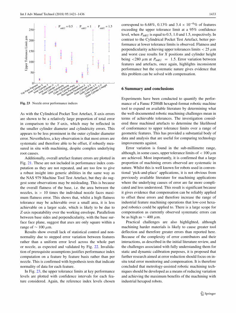
As with the Cylindrical Pocket Test Artefact, X-axis errorsare shown to be a relatively large proportion of total errorin comparison to the Y-axis, which may be reflected inthe smaller cylinder diameter and cylindricity errors. Thisappears to be less prominent in the outer cylinder diametererror. Nevertheless, a key observation is that most errors aresystematic and therefore able to be offset, if robustly mea-sured in situ with machining, despite complex underlyingroot causes.

Additionally, overall artefact feature errors are plotted inFig. 21. These are not included in performance index com-putation as they are not repeated, and are too few to givea robust insight into generic abilities in the same way asthe NAS 979 Machine Tool Test Artefact, but they do sug-gest some observations may be misleading. This is becausethe overall flatness of the base, i.e. the area between thenozzles, is > 10 times the individual nozzle faces maxi-mum flatness error. This shows that, whilst a high flatnesstolerance may be achievable over a small area, it is lessachievable on a larger scale, which is likely to be due toZ-axis repeatability over the working envelope. Parallelismbetween base sides and perpendicularity, with the base sur-face face plane, suggest that axes are only square within arange of ∼ 100 μm.

Results show overall lack of statistical control and non-normality due to stepped error variation between featuresrather than a uniform error level across the whole partor nozzle, as expected and validated by Fig. 22. Invalida-tion of prerequisite assumptions justifies performance indexcomputation on a feature by feature basis rather than pernozzle. This is confirmed with hypothesis tests that indicatenormality of data for each feature.

In Fig. 23, the upper tolerance limits at key performancelevels are plotted with confidence intervals for each fea-ture considered. Again, the reference index levels chosen

correspond to 6.68%, 0.13% and 3.4 × 10−6% of featuresexceeding the upper tolerance limit at a 95% confidencelevel, when PmkU is equal to 0.5, 1.0 and 1.5, respectively. Incontrast to the Cylindrical Pocket Test Artefact, better per-formance at lower tolerance limits is observed. Flatness andperpendicularity achieving upper tolerances limits < 25 μmand worst case results for X positions and cylinder heightbeing <280 μm at PmkU = 1.5. Error variation betweenfeatures and artefacts, once again, highlights inconsistentperformance but the systematic nature gives evidence thatthis problem can be solved with compensation.

6 Summary and conclusions

Experiments have been conducted to quantify the perfor-mance of a Fanuc F200iB hexapod-format robotic machinetool to expand on available literature by determining whatthe well-documented robotic machining challenges mean interms of achievable tolerances. The investigation consid-ered three machined artefacts to determine the likelihoodof conformance to upper tolerance limits over a range ofgeometric features. This has provided a substantial body ofdata and analysis that are useful for comparing technologyimprovements against.

Error variation is found in the sub-millimetre range,although, in some cases, upper tolerance limits of < 100 μmare achieved. Most importantly, it is confirmed that a largeproportion of machining errors observed are systematic innature. Whilst this is well known for robots used in conven-tional ‘pick-and-place’ applications, it is not obvious frompreviously available literature for machining applicationswhere the underlying causes of error are far more compli-cated and less understood. This result is significant becauseit gives evidence that compensation can be reliably appliedto offset these errors and therefore increase the range ofindustrial feature machining operations that low-cost hexa-pod robotics could be applied to. There is a large scope forcompensation as currently observed systematic errors canbe as high as ∼ 400 μm.

Practical challenges are also highlighted, althoughmachining harder materials is likely to cause greater tooldeflection and therefore greater errors than reported here.Because of the complexity of error contributors and theirinteractions, as described in the initial literature review, andthe challenges associated with fully understanding them forstatic and dynamic calibration purposes, it is proposed thatfurther research aimed at error reduction should focus on in-situ total error monitoring and compensation. It is thereforeconcluded that metrology-assisted robotic machining tech-niques should be developed as a means of reducing variationand achieving the maximum benefits of the machining withindustrial hexapod robots.

1434 Int J Adv Manuf Technol (2018) 95:1421–1436

Overall, base case performance has been quantified todetermine how commonly researched robotic machining chal-lenges ultimately relate to achievable tolerances forming abenchmark for process selection and comparing develop-ments against. Potential for substantially tolerance improve-ment has been demonstrated, directing further research.

Acknowledgments The author of this paper would like to acknowl-edge Rolls-Royce Civil Nuclear and the Engineering and Physical Sci-ences Research Council for the provision of funding and to the NuclearAMRC for the access to equipment and technical support. The viewsexpressed in this paper are those of the authors and not necessarilythose of the funding bodies or other organisations mentioned.

Open Access This article is distributed under the terms of theCreative Commons Attribution 4.0 International License (http://creativecommons.org/licenses/by/4.0/), which permits unrestricteduse, distribution, and reproduction in any medium, provided you giveappropriate credit to the original author(s) and the source, provide alink to the Creative Commons license, and indicate if changes weremade.

References

1. Wang Z, Mastrogiacomo L, Franceschini F, Maropoulos P (2011)Experimental comparison of dynamic tracking performance ofiGPS and laser tracker. Int J Adv Manuf Technol 56(1-4):205–213.https://doi.org/10.1007/s00170-011-3166-0

2. Barnfather JD, Goodfellow MJ, Abram TJ (2016) A performanceevaluation methodology for robotic machine tools used in largevolume manufacturing. Robot Comput-Integr Manuf 37:49–56.https://doi.org/10.1016/j.rcim.2015.06.002

3. Jung J-HH, Choi J-PP, Lee S-JJ (2006) Machining accuracyenhancement by compensating for volumetric errors of a machinetool and on-machine measurement. J Mater Process Technol174(1-3):56–66. https://doi.org/10.1016/j.jmatprotec.2004.12.014

4. Weill R, Shani B (1991) Assessment of accuracy in relation withgeometrical tolerances in robot links. CIRP Ann - Manuf Technol40(1):395–399. https://doi.org/10.1016/S0007-8506(07)62015-0

5. Karimi D, Nategh M (2014) Kinematic nonlinearity analysisin hexapod machine tools. Symmetry Reg Accuracy WorkspaceMech Mach Theory 71:115–125. https://doi.org/10.1016/j.mechmachtheory.2013.09.007

6. Kanaan D, Wenger P, Chablat D (2007) Kinematics analysis of theparallel module of the VERNE machine. In: 12th ITFoMM WorldCongress, pp 1–6

7. Bi ZM, Jin Y (2011) Kinematic modeling of Exechon parallelkinematic machine. Robot Comput-Integr Manuf 27(1):186–193.https://doi.org/10.1016/j.rcim.2010.07.006

8. Bi ZM, Wang L (2009) Optimal design of reconfigurable parallelmachining systems. Robot Comput-Integr Manuf 25(6):951–961.https://doi.org/10.1016/j.rcim.2009.04.004

9. Agheli M, Nategh M (2009) Identifying the kinematic parame-ters of hexapod machine tool. World Acad Sci Eng Technol 52:380–385

10. Chanal H, Duc E, Hascoet JY, Ray P (2009) Reduction of a paral-lel kinematics machine tool inverse kinematics model with regardto machining behaviour. Mech Mach Theory 44(7):1371–1385.https://doi.org/10.1016/j.mechmachtheory.2008.11.004

11. Kanaan D, Wenger P, Chablat D (2009) Kinematic analysis of aserial-parallel machine tool. VERNE Mach Mech Mach Theory44(2):487–498. arXiv:0811.4733, https://doi.org/10.1016/j.mechmachtheory.2008.03.002

12. Fassi I, Wiens GJ Multiaxis machining: PKMs and traditionalmachining centers. J Manuf Process 2 1. https://doi.org/10.1016/S1526-6125(00)70008-9

13. Halaj M, Kurekova E (2009) Positioning accuracy of non-conventional production machines—an introduction. In: Proceed-ings of XIX IMEKO World Congress, Lisbon, pp 2099–2102

14. Zhang HZH, Wang JWJ, Zhang G, Gan ZGZ, Pan ZPZ,Cui HCH, Zhu ZZZ (2005) Machining with flexible manipu-lator: toward improving robotic machining performance. Proc2005 IEEE/ASME Int Conf Adv Intell Mechatron 0:1127–1132.https://doi.org/10.1109/AIM.2005.1511161

15. Doukas C, Pandremenos J, Stavropoulos P, Foteinopoulos P,Chryssolouris G, Mourtzis D, Stavropoulos P, Foteinopoulos P,Chryssolouris G (2012) On an empirical investigation of the struc-tural behavior of robots. 45th CIRP Conf Manuf Syst 3:501–506.https://doi.org/10.1016/j.procir.2012.07.086

16. Pandremenos J, Doukas C, Stavropoulos P, Chryssolouris G(2011) Machining with robots: a critical review. In: (DET2011),7th international conference on digital enterprise technology,Athens, Greece, pp 614–621. ISBN 978–960–88104–2–6

17. Dumas C, Caro S, Garnier S, Furet B (2011) Joint stiffness iden-tification of six-revolute industrial serial robots. Robot Comput-Integr Manuf 27(4):881–888. https://doi.org/10.1016/j.rcim.2011.02.003

18. Sornmo O, Olofsson B, Robertsson A, Johansson R (2012)Increasing time-efficiency and accuracy of robotic machin-ing processes using model-based adaptive force control. 10thIFAC Symp Robot Control - SYROCO 2012 45(22):543–548.https://doi.org/10.3182/20120905-3-HR-2030.00065

19. Matsuoka SI, Shimizu K, Yamazaki N, Oki Y (1999) High-speed end milling of an articulated robot and its characteristics.J Mater Process Technol 95(1-3):83–89. https://doi.org/10.1016/S0924-0136(99)00315-5

20. Lehmann C, Halbauer M, Euhus D, Overbeck D (2012) Millingwith industrial robots: strategies to reduce and compensate processforce induced accuracy influences. IEEE Int Conf Emerg Tech-nol Fact Autom, ETFA 17:1–4. https://doi.org/10.1109/ETFA.2012.6489741

21. Olofsson B, Sornmo O, Schneider U, Barho M, Robertsson A,Johansson R (2012) Increasing the accuracy for a piezo-actuatedmicro manipulator for industrial robots using model-based non-linear control. 10th IFAC Symp Robot Control - SYROCO2012 45(22):277–282. https://doi.org/10.3182/20120905-3-HR-2030.00116

22. Abele E, Weigold M, Rothenbucher S (2007) Modeling andidentification of an industrial robot for machining applications.CIRP Ann - Manuf Technol 56(1):387–390. https://doi.org/10.1016/j.cirp.2007.05.090

23. Bouzgarrou BC, Fauroux JC, Gogu G, Heerah Y (2004) Rigidityanalysis ofT3R1 parallel robot with uncoupled kinematics. In: Pro-ceedings of the 35th international symposium on robotics, no. 5,international federation of robotics, Paris, pp 5–10

24. Li Y, Liu H, Zhao X, Huang T, Chetwynd DG (2010) Design ofa 3-DOF PKM module for large structural component machin-ing. Mech Mach Theory 45(6):941–954. https://doi.org/10.1016/j.mechmachtheory.2010.01.008

25. Wu H, Handroos H, Kovanen J, Rouvinen A, Hannukainen P,Saira T, Jones L (2003) Design of parallel intersector weld/cutrobot for machining processes in ITER vacuum vessel. FusionEng Des 69(1-4):327–331. https://doi.org/10.1016/S0920-3796(03)00066-8

Int J Adv Manuf Technol (2018) 95:1421–1436 1435

26. Wu H, Handroos H, Pessi P, Kilkki J, Jones L (2005) Developmentand control towards a parallel water hydraulic weld/cut robot formachining processes in ITER vacuum vessel. Fusion Eng Des 75-79:625–631. https://doi.org/10.1016/j.fusengdes.2005.06.304

27. Pessi P, Wu H, Handroos H, Jones L (2007) A mobile robotwith parallel kinematics to meet the requirements for assemblingand machining the ITER vacuum vessel. Fusion Eng Des 82(15-24):2047–2054. https://doi.org/10.1016/j.fusengdes.2007.06.012

28. Pan Z, Zhang H (2009) Improving robotic machining accuracyby real-time compensation. In: ICROS-SICE International JointConference, pp 4289–4294

29. Pan Z, Zhang H, Zhu Z, Wang J (2006) Chatter analysis of roboticmachining process. J Mater Process Technol 173(3):301–309.https://doi.org/10.1016/j.jmatprotec.2005.11.033

30. Olabi A, Bearee R, Gibaru O, Damak M (2010) Feedrate plan-ning for machining with industrial six-axis robots. Control Eng Pract18(5):471–482. https://doi.org/10.1016/j.conengprac.2010.01.004

31. Turek P, Jedrzejewski J, Modrzycki W (2010) Methods of machinetool error compensation. J Mach Eng 10(4):5–25. https://doi.org/10.1016/j.procir.2013.06.078

32. Gong C, Yuan J, Ni J (2000) Nongeometric error identifica-tion and compensation for robotic system by inverse calibration.Int J Mach Tools Manuf 40(14):2119–2137. https://doi.org/10.1016/S0890-6955(00)00023-7

33. Kamrani AK, Wei C-CC, Wiebe HA, Wei C-CC (1995) Ani-mated simulation of robot process capability. Integr Manuf Syst28(1):23–41. https://doi.org/10.1108/09576069410056723

34. Antunes Simoes JFCP, Coole TJ, Cheshire DG, Pires AR (2003)Analysis of multi-axis milling in an anthropomorphic robot,using the design of experiments methodology. J Mater Pro-cess Technol 135(2-3 SPEC.):235–241. https://doi.org/10.1016/S0924-0136(02)00908-1

35. Olabi A, Bearee R, Nyiri E, Gibaru O (2010) Enhanced tra-jectory planning for machining with industrial six-axis robots.Proc IEEE Int Conf Ind Technol 18:500–506. https://doi.org/10.1109/ICIT.2010.5472749

36. Zargarbashi S, Khan W, Angeles J (2012) The Jacobian condi-tion number as a dexterity index in 6R machining robots. RobotComput-Integr Manuf 28(6):694–699. https://doi.org/10.1016/j.rcim.2012.04.004

37. Zargarbashi S, Khan W, Angeles J (2012) Posture optimization inrobot-assisted machining operations. Mech Mach Theory 51:74–86. https://doi.org/10.1016/j.mechmachtheory.2011.11.017

38. Young K, Pickin CG (2001) Speed accuracy of the modernindustrial robot. Ind Robot: Int J 28(3):203–212. https://doi.org/10.1108/01439910110389362

39. Chen Y, Dong F (2012) Robot machining: recent developmentand future research issues. Int J Adv Manuf Technol:1489–1497.https://doi.org/10.1007/s00170-012-4433-4

40. Tunc LT, Barnfather JD (2014) Effects of hexapod robot dynam-ics in milling. In: 11th International Conference on High SpeedMachining, vol 1269. MM Science Journal, Prague, pp 1–8

41. Tunc LT, Shaw J (2015) Experimental study on investigationof dynamics of hexapod robot for mobile machining. Int J AdvManuf Technol 84(5):817–830. https://doi.org/10.1007/s00170-015-7600-6

42. Tunc LT, Shaw J (2016) Investigation of the effects of Stew-art platform-type industrial robot on stability of robotic milling.Int J Adv Manuf Technol 0:1–11. https://doi.org/10.1007/s00170-016-8420-z

43. ISO 8688-2 (1989) Tool life testing in milling - Part 2: End milling44. Taylor F (1907) On the art of cutting metals. In: Transactions

of ASME, vol 28, New York, pp 1–1198. https://doi.org/10.1038/scientificamerican01051907-25929bsupp

45. Chen J, Liu W, Deng X, Wu S (2016) Tool life and wear mech-anism of WC-5TiC-0.5VC-8Co cemented carbides inserts whenmachining HT250 gray cast iron. Ceram Int 42(8):10037–10044.https://doi.org/10.1016/j.ceramint.2016.03.107

46. Panda A, Duplak J, Vasilko K (2012) Analysis of cutting toolsdurability compared with standard ISO 3685. Int J Comput TheoryEng 4(4):621–624. https://doi.org/10.7763/IJCTE.2012.V4.544

47. Tschatsch H (2009) Applied machining technology, Springer,London. arXiv:1011.1669v3, https://doi.org/10.1007/9783642010071

48. Cheng K (2009) Machining dynamics: fundamentals, applicationsand practices. Springer, London

49. Davim JP (2011) Machining of hard materials. Springer, London50. Davim JP (2008) Machining: fundamentals and recent advances.

Springer, London51. Wang J, Zhang H, Pan Z (2016) Machining with flexible manip-

ulators: critical issues and solutions. In: Huat LK (ed) Indus-trial robots, programming and application, InTech, 2006, Ch. 26,pp 515–526. https://doi.org/10.5772/4914

52. Razali NM, Wah YB (2011) Power comparisons of Shapiro-Wilk,Kolmogorov-Smirnov, Lilliefors and Anderson-Darling tests. JStat Model Anal 2(1):21–33

53. Stephens MA (1974) EDF statistics for goodness of fit and somecomparisons. J Amer Stat Assoc 69(347):730–737. https://doi.org/10.1080/01621459.1974.10480196

54. Stephens MA (1976) Asymptotic results for goodness-of-fitstatistics with unknown parameters. Ann Stat 4(2):357–369.https://doi.org/10.1214/aos/1176343411

55. Sakia RM (1992) The box-cox transformation technique: a review.Statistician 41(2):169. https://doi.org/10.2307/2348250

56. Hosseinifard SZ, Abbasi B, Ahmad S, Abdollahian M (2009) Atransformation technique to estimate the process capability indexfor non-normal processes. Int J Adv Manuf Technol 40:512–517.https://doi.org/10.1007/s00170-008-1376-x

57. Bianchi G, Cagna S, Cau N, Paolucci F (2014) Analysis ofvibration damping in machine tools. Procedia CIRP 21:367–372.https://doi.org/10.1016/j.procir.2014.03.158

58. Grossi N, Scippa A, Sallese L, Sato R, Campatelli G (2015)Spindle speed ramp-up test: a novel experimental approach forchatter stability detection. Int J Mach Tools Manuf 89:221–230.https://doi.org/10.1016/j.ijmachtools.2014.11.013

59. Zhang H-TT, Wu Y, He D, Zhao H (2015) Model predic-tive control to mitigate chatters in milling processes with inputconstraints. Int J Mach Tools Manuf 91:54–61. https://doi.org/10.1016/j.ijmachtools.2015.01.002

60. Moradi H, Vossoughi G, Behzad M, Movahhedy MR (2015)Vibration absorber design to suppress regenerative chatter innonlinear milling process: application for machining of can-tilever plates. Appl Math Modell 39(2):600–620. https://doi.org/10.1016/j.apm.2014.06.010

61. Li KM, Liang SY (2007) Modeling of cutting forces in near drymachining under tool wear effect. Int J Mach Tools Manuf 47(7-8):1292–1301. https://doi.org/10.1016/j.ijmachtools.2006.08.017

62. BSENISO 10360-2 (2009) Geometrical product specifications—acceptance and reverification tests for coordinate measuring machines(CMM) Part 2: CMMs used for measuring linear dimensions

63. AiA/NAS NAS979 (1969) Uniform cutting tests—NAS seriesmetal cutting equipment specifications

64. Gagnol V, Le TP, Ray P (2011) Modal identification of spindle-tool unit in high-speed machining. Mech Syst Signal Process25(7):2388–2398. https://doi.org/10.1016/j.ymssp.2011.02.019

65. Zaghbani I, Songmene V (2009) Estimation of machine-tooldynamic parameters during machining operation through opera-tional modal analysis. Int J Mach Tools Manuf 49(12-13):947–957. https://doi.org/10.1016/j.ijmachtools.2009.06.010

1436 Int J Adv Manuf Technol (2018) 95:1421–1436

66. Li B, Cai H, Mao X, Huang J, Luo B (2013) Estimation of CNCmachine-tool dynamic parameters based on random cutting exci-tation through operational modal analysis. Int J Mach Tools Manuf71:26–40. https://doi.org/10.1016/j.ijmachtools.2013.04.001

67. Kovarık M, Sarga L (2014) Process capability indices fornon-normal data. WSEAS Trans Business Econ 11:419–429.https://doi.org/10.1080/0898211000896.2614

68. BSISO 22514-3 (2008) Statistical methods in process manage-ment capability and performance—part 3: machine performancestudies for measured data on discrete parts

69. Barnfather JD, Goodfellow MJ, Abram TJ (2017) Positionalcapability of a hexapod robot for machining applications. IntJ Adv Manuf Technol 89(1):1103–1111. https://doi.org/10.1007/s00170-016-9051-0