Embed Size (px)
Citation preview

1
Accuracy, Timeliness, and Managerial Discretion of Fair Value Pricing:
Evidence from the US Banking Industry
Andrew Jing Liu
Harvard Business School
December 2017
ABSTRACT: This paper investigates how recent institutional developments impact the potential
channels, and thus available discretion, by which managers can manipulate reported fair values.
First, I use extensive field research to document the mechanisms used by banks to procure and
report fair values—particularly incorporating the impact of the 2011 FINRA’s Trade Reporting
and Compliance Engine (TRACE), and concurrent increase in independent third-party vendors.
Key insights include that (i) banks predominantly apply third-party vendors’ feeds to generate
financial statements (with nearly 100% of vendors’ feeds passing automatically to reported
financial statements, with only rare adjustments); and (ii) external auditors predominantly relying
on different vendors’ prices to verify and challenge banks’ inputs. Second, I employ three
proprietary datasets of daily financial-instrument level pricing—capturing both TRACE and
third-party vendors—to document the following insights. I find that vendors’ evaluated prices
dominate historical costs in all performance metrics, confirming they provide a more accurate,
objective, and reliable proxy for fair value than historical cost. I also find that vendors’ fair
values are value-relevant and account for 90% of the trade-to-trade price variance, creating an
upper bound on managerial discretion (of only 15% of the original level). Finally, I find that
bank managers respond to these newly imposed constraints by alternatively engaging in more
spoofing-transaction based fair value manipulations: suggesting this is a likely (even primary)
channel by which manipulation can be attained. Overall, the evidence suggests that fair values,
particularly after the above institutional developments, appear less subjective, less costly to
implement, and more convenient for auditors to verify and challenge, than the literature has
previously reported.
JEL Classification: M41, G12, G18
Keywords: fair value accounting, managerial discretion, third party vendors, FINRA, TRACE,
SFAS 157, available-for-sale assets
Andrew Jing Liu is a doctoral candidate at Harvard Business School. I thank my dissertation committee Dennis Campbell
(Chair), Krishna Palepu (Co-Chair), Eddie Riedl, and Adi Sunderam for their continuous guidance and mentorship. I am
grateful to the following for useful discussions: Paul Healy, Krishna Palepu, Robert Kaplan, Ross Watts, Eugene Soltes,
Aiyesha Dey, Ethan Rouen, Burton Hollifield, Jens Dick-Nielsen, Marco Rossi, Vladimir Atanasov, and Nils Friewald,
Jessica Matheron, Ian Blance, Mark Adelson, Virginie O'Shea, and seminar participants at Harvard Business School for
helpful comments. All errors are solely my own responsibility. Contact author: Andrew Jing Liu [email protected].

2
1. Introduction
Prior research provides strong evidence of managerial manipulation in the reporting of
fair value estimates (Benson and Teclezion 2007; Benston 2008). The evidence appears
particularly compelling in the context of fair value estimates based on inputs not directly
observed from the markets: so-called Level 2 and 3 fair value estimates. Benston (2008)
summarizes this view: “fair values other than those taken from quoted prices could be readily
manipulated by opportunistic and overoptimistic managers, would be costly to make, and very
difficult for auditors to verify and challenge.” The related and on-going debate between fair
value and historical cost reflects an implicit yet crucial assumption: no accurate, objective, and
reliable alternative approaches are available to estimate fair value other than historical cost.
Much of the prior research relies on quarterly Level 2 and 3 aggregated data prior to
2011. Critically, this research does not reflect recently enacted institutional changes surrounding
the daily security-level pricing and reporting process itself: i.e., how individual daily fair values
are generated, validated, aggregated to the general ledger, and ultimately reported in the financial
statements. This paper fills this gap in two ways. First, I use field research to extensively
document the mechanisms used by banks to procure and report fair values, incorporating two key
recent institutional developments intended to improve the fair value reporting process:
independent third-party vendors and FINRA’s Trade Reporting and Compliance Engine
(TRACE). Second, I use three proprietary datasets of daily financial instrument-level—capturing
both TRACE and vendor pricing—to evaluate how these new developments affect managerial
discretion and the potential channels by which to manipulate fair values. Thus, this study
reexamines prior literature’s general conclusions on discretion in banks’ reporting of fair values,
including the novel and undocumented impact of TRACE and third-party vendor pricing.

3
The US banking industry is an ideal setting for this research, as banks hold large numbers
of financial instruments subject to fair value accounting. To maximize instruments ex ante likely
subject to greater managerial discretion, I focus on the infrequently traded structured credit
products (SCP), which includes: asset-backed securities (ABS); collateralized mortgage
obligations (CMO); mortgage-backed securities (MBS); and to-be-announced (TBA) securities.1
SCPs are one of the largest but least-studied segments of the financial market, with valuation
process that are poorly understood, in part owing to their complexity and low trading activity.2
For my qualitative field research, I interview 100+ professionals from banks, third-party
vendors, external auditors, FINRA, broker-dealers, and BWIC firms.3 I also shadow fair value
professionals for one complete financial statement generating cycle, including attendance at a
quarterly valuation oversight committee meeting. My quantitative research consists of empirical
tests using three proprietary datasets acquired from the vendors and TRACE, with data spanning
2011-2015. Descriptively, I find that the average number of trades per security over the 4.5-year
sample period is 5.17, averaging 107 days between adjacent trade dates. Critically, during the
past 10 years, independent third-party vendors have begun to fill in the price gaps between
adjacent trades, by supplying daily security-level evaluated prices.
Through my field research, three key insights emerged. First, banks principally
“outsource” their pricing functions to independent third-party vendors. In particular, banks
predominantly pass through vendors’ pricing feeds directly to their reported financial statements,
with (at most) occasional adjustments: almost all banks that I interviewed pass nearly 100% of
vendors’ feeds automatically to their general ledger. Second, external auditors also
1 A to-be-announced (TBA) is a forward contract for a homogeneous pool of MBS pass-throughs. 2 At 2016, there are $8.9 trillion outstanding in MBS; this compares to $13 ($8.9) [$3.8] trillion in the Treasury (corporate
bond) [municipal bond] markets. Data are from www.sifma.org/research/statistics.aspx. 3 Bid Wanted in Competition (BWIC) is a system, in which an institutional investor submits its bid list to various dealers.
Dealers make bids on the listed securities, with those having the highest bids then contacted.
4
predominantly rely on different vendors’ pricing feeds and expertise to verify and challenge
banks’ reported fair values; this includes directly contacting their clients’ vendors for further
information and validation. Third, these recent institutional developments allow me to
characterize the three potential channels by which managers can manipulate fair values: strategic
vendor selection or cherry picking among vendors (Channel One); manipulating general ledger's
numbers and/or strategically timing the recognition of unrealized gains/losses (Channel Two);
and spoofing the vendors—that is, manipulating vendors’ prices through purposefully “spoofed”
transactions that are subsequently cancelled (Channel Three).
My quantitative research then supplements the above field research observations by
providing three pieces of supporting evidence that managerial discretion over fair values is
constrained by TRACE and vendor pricing in Channels One and Two, with Channel Three
appearing to be the only mechanism through which any viable managerial manipulation can
occur. First, I find that the evaluated prices from different vendors are quite similar and show
little systemic biases. In particular, pricing differences between two vendors’ feeds have thin-
tailed distributions, indicating that extreme pricing differences are less likely to occur compared
to corresponding normal distributions. This evidence suggests that managerial discretion via
strategic vendor selection (Channel One) is likely quite limited.
Second, I assess vendor performance by comparing its pricing feeds to both the historical
costs and the next trade prices. I find that vendors’ evaluated prices dominate historical costs in
all performance metrics, including variance reduction, model bias, forecast error, mean error, and
directional correctness. In particular, vendors’ fair values are value-relevant, accounting for 85%
of the price movements subsequent to the initially reported historical costs, and also explain 90%
of the inter-trade price variance. This evidence suggests that vendors’ prices provide effective
5
valuation reference points for the next trades; and thus appear to be a more accurate, objective,
and reliable proxy for fair value than historical cost. Furthermore, the ubiquitous availability of
vendors’ prices to all market participants (auditors, investors, and regulators) suggests an upper
bound on managerial discretion through Channel Two, only 15% of the original level.
Third, focusing on a particular type of “Cancelled-Single” trades, I investigate whether
bank managers purposefully use cancellations to spoof vendors’ prices. I find that vendors’
prices react promptly and significantly to the initial posted trades, yet only gradually and less
markedly to the later cancellations. This asymmetric response gives bank managers a potential
means to artificially inflate/deflate vendors’ prices and then enjoy the ensuing favorable
temporarily-mispriced fair values. I also find that both the scope and extent of the Cancelled-
Single trades are limited. Together, with corroborating evidence from additional tests, vendors’
asymmetric response to the original trades and later cancellations provides evidence that bank
managers engage in limited spoofing-transaction-based fair value manipulations through
Channel Three.
This study makes four contributions. First, the field research provides a rich descriptive
analysis surrounding banks’ daily fair value pricing practices as well as the undocumented
impact of TRACE and vendors’ pricing on managerial discretion. Thus, it builds on prior
research examining earnings management of banks, including fair value measurements (Beatty
and Harris 1999; Beatty et al. 2002; Ettredge et al. 2010; Fiechter and Meyer 2010; Liao et al.
2010; and Song et al. 2010). Second, the proprietary TRACE and vendor datasets allow
investigation of daily fair values for individual securities; this improves previous research relying
on quarterly financial statement data at an aggregate portfolio level (Level 2 and 3) (Beatty et al.
2002; Thomas and Zhang 2002; Bens et al. 2002, 2003; Kanagaretnam et al. 2004; and

6
Roychowdhury 2006). Third, it is the first to suggest that vendors’ evaluated prices dominate
historical costs in all performance metrics, as well as to identify the related point estimate (85%)
reduction in bank managers’ discretion. Finally, it provides a framework of three channels by
which managers can potentially manipulate fair values, with empirical evidence that Channel
Three (spoofing the vendors) appears the most viable for feasible managerial manipulation.
Section 2 reviews prior research. Section 3 discusses the qualitative field research.
Section 4 develops the hypotheses and research design. Section 5 presents the empirical results.
Section 6 concludes.
2. Literature Review
This study follows two streams of research: fair value accounting and third-party
vendors/TRACE. Regarding fair value reporting, the debate has been long-lived and
inconclusive. Early studies primarily focus on the value relevance of fair values (Barth 1994,
1995; Nelson 1996; Barth et al. 1996; Liang and Riedl 2011). Recent studies have focused on
fair value disclosures (Liao et al. 2010; Song et al. 2010; Riedl and Serafeim 2011). Some
researchers have expressed concerns that fair values give managers more discretion (Benston
2008; Ryan 2008; Martin et al. 2006), leading to research that examines how fair values affect
earnings manipulation and auditing (Chen et al. 2010; Ettredge et al. 2010; Fiechter and Meyer
2010; Heflin and Valencia 2012). Taken together, prior research from both sides of the debate
believe that fair values (especially level 2 and level 3), are subject to managerial manipulation.
To my best knowledge, there has been no prior research on third-party vendors and
TRACE in the accounting literature. Prior research on TRACE has come from finance and have
focused exclusively on corporate bonds (Edwards et al. 2007; Goldstein et al. 2007; Green et al.
2007b; Mahanti et al. 2008; Bao et al. 2011; Jankowitsch et al. 2011; Lin et al. 2011; Nashikkar

7
et al. 2011; Dick-Nielsen et al. 2012; Feldhutter 2012; Friewald et al. 2012; and Ronen and Zhou
2013). Collectively, these studies found that TRACE has effectively increased pre-trade
transparency, reduced investor transaction costs, and improved valuation precision.
3. Qualitative Field Research
This section overviews the insights obtained from my qualitative field research on the
process by which fair values for bank financial instruments are obtained.4 For brevity, the terms
of “banks”, “vendors”, and “auditors” in this section reflect “banks, (vendors, and auditors) that I
interviewed.” This section discusses the following: vendors, TRACE, auditors, and US banks.
Figure 1 provides an overall roadmap for the following field research discussions. It
illustrates the various components inside the black box, and how trade information flows through
these components from bank managers to banks’ financial statements.
I would like to start the field research discussion with an analogy. A bank’s daily fair
value practice is like the valuation of a car dealership: each car on the parking lot is analogous to
an individual security on the balance sheet; pricing companies (Edmonds and Autobytel) are
analogous to third-party vendors; and a hypothetical centralized nation-wide transaction
reporting system is analogous to TRACE. According to prior literature, managers have
unchecked pricing discretions and can easily manipulate prices to their advantages. However, in
the following sections, I argue that financial securities, just like cars, are quite standardized and
well parameterized. The valuation of a non-traded vehicle can be reasonably inferred by cross-
referencing to transactions of similar cars through a relational network of valuation inputs
(model, mileage, vintage, trim, location, etc.). If prices provided by Autobytel can account for a
significant portion of the ensuing price movements since the historical costs, and thus can serve
4 This section only outlines the key insights necessary for the subsequent empirical analysis and discussions. For more a more
detailed discussion, I refer readers to Liu and Riedl (2017).

8
as accurate and reliable up-to-date valuation reference points for the next trades, then market
participants may prefer Autobytel’s prices to historical costs. Therefore similarly, bank
management’s discretion over fair values will be significantly constrained, as long as the widely
available vendors’ evaluated prices can accurately and reliably predict the next trade prices.
I also want to emphasize the importance of the field research from a perspective of causal
inference. According to Gow et al. (2016), accounting research would benefit from “draw(ing)
plausible causal inferences by establishing clear mechanisms, or causal pathways.” The authors
also warn against indiscriminately treat difference-in-difference method as “quasi-experimental”.
In-depth field research, on the other hand, can open up the black box, improve our understanding
of causal mechanisms, and pinpoint clearer cause-effect pathways. Suppose my field research
suggests that the first-order effects and the causal mechanism for decrease in managerial
discretion come directly from vendors’ effective performance (i.e. vendors’ prices provide
reliable and accurate up-to-date predictors for the next trades). If we can further empirically
establish the validity of this pinpointed direct causal pathway, then comparing managerial
discretion in the pre- and post- TRACE/vendor periods would only add additional evidence
because it can only provide a macro-level aggregated association, not mechanism-specific
causation. Another way to look at the association/causation distinction is that vendors’ effective
performance will surely lead to a decrease in managerial discretion; while both the association
(significant regression results) and lack of association (insignificant results) can be driven by
unobserved confounding variables. There is still a heavy burden on researchers to explain why
they believe their models have “controlled away” all spurious associations. Therefore, this study
will mainly focus on using field research to identify the direct causal mechanism (i.e. vendors’

9
effective performance leads to a decrease in managerial discretion) and using empirical tests to
establish the validity of this causal pathway.
The following field research section is thematically organized into four parts:
independent third-party vendors, FINRA’s TRACE, external auditors, and US banks.
3.1.Third-party Vendors
Evaluated pricing services (EPS), also called independent third-party vendors, have been
one of the fastest growing financial intermediaries since the 2008 financial crisis. The entire
pricing service sector is estimated to be a one-billion-dollar business.5 Currently the “big four”
EPSs are Intercontinental Exchange (ICE), IHS Markit, Thomson Reuters, and Bloomberg.
Competition among vendors for better performance is fierce,6
because client valuation
committees will normally award business to a vendor based on its relative performance.7
A vendor’s main business function is to provide daily evaluated security-level prices.
Nowadays, major vendors provide pricing services covering almost the entire universe of
financial securities. For thinly traded complex securities such as SCPs, vendors typically reply
on algorithm based valuation models (aka “bucketing” pricing), in which vendors compile
transaction prices from various sources and construct a pricing matrix, from which key
characteristics such as credit spreads to specific benchmarks are calculated and updated as new
data become available. Securities are further segregated into different buckets by characteristics
such as term, rating, size, and so on. Once spread levels have been stratified, similar securities
can be priced relative to a benchmark using the matrix. Normally, each risk-weighted bucket
contains 10 to 15 securities. These buckets are dynamic and constantly changing to reflect the
5 Executives from the three largest EPS gave the author the same estimate in separate occasions. 6 Please refer to Table 3 for illustration of commonly used performance metrics. 7 Competition among vendors is mainly centered on winning new clients because once clients have built the corresponding IT
infrastructure and interface to one vendor, it is quite costly for them to switch to another one.

10
most recent market conditions.8 All the inputs
9 used to make a pricing decision are stored and
documented, allowing for timely price challenge and audit responses. In addition to these “robot-
like” algorithm-based models, vendors also have a large group of evaluators, who are mostly
former traders from major banks or broker/dealers. Evaluators are in almost constant contact
with the trading desks of broker-dealers in order to get a current valuation. Evaluators have
similar skills and market knowledge as traders/dealers; however, they are generally more
informed than bank traders because they can see almost all prices and quotes on the market,
while traders only see the ones from their own firms.
According to vendors’ executives, vendor’s responsibility is not necessarily to “seek the
intrinsic theoretical values” of the underlying security. Rather, vendors are “just a messenger” to
incorporate all available information as quickly and objectively as they can. They then pass on to
clients in the form of a single price, at which “the next transaction is mostly likely to occur for
this particular moment.”
Vendors’ clients include buy-side asset managers, hedge funds, insurance companies,
government agencies, auditors, and banks. Mutual funds are, by far, the most important clients,
and are the driving forces behind the vendors’ business, because of their needs to calculate daily
net asset values. Banks, on the other hand, are quite low in the pecking order. Banks most often
outsource valuation to vendors, and enrolled in subscriptions paid for by their buy-side asset
management arms. Since this “coleslaw” option10
requires no upfront investment or ongoing
maintenance, it is a cost-effective solution that has great appeal. Another important reason banks
8 Bucketing” pricing methodology is a somewhat updated/upgraded “2.0” version of the now outdated “matrix pricing”, in that
the buckets are dynamic, rather than static as in the matrix pricing, which has fixed “buckets”. 9 Observable inputs include: pool-specific characteristics loan age/size, and credit quality of borrowers; yields for Treasury
securities of various maturities; a range of spread and discount margin assumptions; floating rate indices (LIBOR); structural
and waterfall features of each bond; and recent trading and bidding activity for bonds with similar collateral characteristics. 10 One bank manager the author interviewed joked that “bank’s subscription to vendors’ services is only the coleslaw of a meal,
asset managers are the real steak.”
11
use third party vendor pricing is convenience. Daily batch files of the pricing feeds sent from the
vendors are easily incorporated into banks’ back-office platforms. Thus, contrary to the current
view of literature, vendors’ pricing services are cost-saving and operationally easy to implement.
Vendors deliver not just the evaluated prices, but also all of the security level associated
valuation assumptions and inputs. For some SCPs, the delivered pricing files have around 100
field columns, including bid, mid, ask, spread, pre-payment speed, liquidity, spread to swaps,
discount margin, Z spread, transaction information from previous trades, etc. With this
information, clients have near-complete access to the “whole story and history” of the security
and the relational networks to similar securities via implied assumptions and inputs.11
The most relevant institutional mechanisms are the “law of single price” principle and
“challenge mechanism”. All the third-party vendors embrace the same “law of single price”
principle, which stipulates that for a particular point in time, the same security must be identified
with the same evaluated price to all clients. Generally, one security can be held by more than one
institution, either on the asset or liability sides, either by the long or short positions. As a result
of these counteracting valuation incentives, vendors don’t have systemically-biased valuation
incentives. In the following quantitative sections, I will conduct further empirical tests on
whether vendors’ prices are systemically biased (H2).
All of the vendors have established challenge processes for their clients to submit
inquirers regarding evaluations. In a challenge, the client presents a disagreement with vendors’
evaluated price regarding a specific security. Upon receipt of the challenge, vendors may affirm
the current evaluation, or amend the evaluation on a going-forward basis. This “no back-fill”
mechanism puts limits on managerial discretion. If a bank challenges and wins, current day
11 Most vendors have four fixed time deliveries: 10:00AM NY time, London Close, 3:00PM NY time, and 4:00PM NY time.
And the clients can choose which batch file(s) they want to subscribe to.
12
prices stay the same; updated information is incorporated on the next day’s prices to all clients
(not only to the one who issued the challenges). All challenges are fully documented and most
challenges are responded to within 24 hours.
In my field research, I interviewed one vendor that receives 5-25 challenges per month
from each of its clients and wins about 70% of all the challenges. Another vendor only amends
and makes forward adjustments on 10-15% of all the challenges it receives. One bank that I
spoke with and whose valuation committee meeting I attended, issues 15-30 challenges per
month, with vendors winning about 75% of these challenges. At the particular committee
meeting that I attended, more than 99% (dollar value) of the fair values were un-adjusted and
flew to the 10Q; less than 1% were adjusted.
In addition to providing daily evaluated prices, third-party vendors have other channels to
increase market transparency, including message parsing, sector-level time series reports,
transparency metrics, and market summary statistics. One important such channels is the
securitized products indices owned and administered by vendors. For example, Markit provides
synthetic tradable indices for different collateral types, including ABX for non-agency RMBS,
MBX for agency RMBS, CMBX for non-agency CMBS, etc. Through these indices, investors
can gain insights into the performance of the relevant SCP sectors. These SCP indices are among
the first attempts to allow investors to gauge market sector-aggregate sentiments and trade risks
that closely mirror the current credit conditions of underlying sector, so that specific interest
spreads can be applied to each risk class.
Another interesting observation worth noting is that from vendors’ perspective, there are
no distinctions between level 2 and level 3 fair values. A security, classified as level 3 by a
client, does not necessarily incur more time and efforts for the vendor to evaluate, nor does it

13
necessarily imply a less accurate and effective evaluated price. The classification occurs not at
the vendors’ upstream production level, but at the clients’ downstream consumption level. If this
is indeed the case, then the current distinction between level 2 and level 3 fair values might not
be as evident as the literature previously has reported (Ettredge et al. 2010; Fiechter and Meyer
2010; Song et al. 2010).
3.2.FINRA’s TRACE
Financial Industry Regulatory Authority (FINRA) is a private and self-regulatory
organization that regulates member broker/dealer firms and exchange markets.12
All firms,
dealers, and brokers that sell securities to the public must be registered and licensed by FINRA.
Trade Reporting and Compliance Engine (TRACE) is the FINRA-developed vehicle that
facilitates the mandatory reporting of secondary market transactions. SCPs are traded exclusively
over-the-counter (OTC) via a dealer network as opposed to on a centralized exchange. Since
May 16, 2011, virtually all trades in the SCP market have been required to be reported to
TRACE by broker/dealers, most of the time within 15-60 minutes of the time of execution.13
Almost all trades reported to TRACE are disseminated within 15 minutes after being reported.
Though TRACE has been collecting all transaction data since May 16, 2011, FINRA has been
disseminating this information to the market in different phases (staged dissemination).14
3.3.External Auditors
I interviewed both third-party vendors and auditors. From the vendors’ perspective, audit
firms are among the most important subscribers and users of the pricing services. In fact,
12 FINRA was formed in July 2007 as a result of the merger of NASD and the member regulation, enforcement and arbitration
operations of NYSE. 13 Please refer to Table 1 Panel D for more details. 14 Please refer to Table 1 Panel B for more details on TRACE’s staged dissemination schedule.

14
responding to inquiries from audit firms is one of the largest components of a vendor’s daily
work. From the auditor’s perspective, audit firms overwhelmingly use third-party vendors for
their pricing feeds and rely on these feeds to verify and challenge banks’ inputs to their financial
statements. Auditors not only have access to the necessary technical support from their own
vendor, but also can directly contact their clients’ (aka banks’) vendor for further information
and verification. The “Big Four” also have their own centralized valuation teams, through which
an auditor can access to not only multiple vendors’ pricing feeds on one particular security, but
also all other auditing teams’ valuation opinions on similar securities.
If this is indeed the case, we need to revisit and rethink the conclusions on the
interactions between auditors and banks from prior literature. The surface-level tug-of-war
between auditors and bank managers, might essentially be a fight between two sets of pricing
feeds: one used by banks from one vendor, and the other used by auditors from a different
vendor. In the following empirical analysis sections, I will further compare fair value prices from
two different vendors (H1).
3.4.US Banks
Untabulated statistics15
reveal that the majority of the fair values are of level 2 (92.9% of
the total fair value assets and 21.6% of liabilities); and available-for-sale (AFS) are the largest
component of fair value assets (69.6%). In 2016, out of the total 265 public banks, 188 banks
disclosed that they either “100% all pass-through without any adjustments”, or “almost all 100%
pass-through”, or use the following words to describe their usage of vendors’ pricing feeds:
“most of”, “majority”, “primarily”, “predominantly”, “occasionally adjust”, “substantial”. These
15 For more a more detailed discussion, I refer readers to Liu and Riedl (2017).

15
188 banks’ AFS2 and AFS316
represent 83% and 96% of AFS2 and AFS3 of the entire
population, respectively.
I focused on the largest 40 US banks and was able to interview more than 50
professionals from 11 banks. These professionals include CFOs, controllers, traders, fair value
committee members, valuation team members, and internal auditors. The average of the total
assets of these 11 banks combined would rank 20th
within the top 40 banks. I also shadowed fair
value professionals for one complete financial statement generating cycle at one bank, which is
the largest of the 11 banks.17
I also attend its quarterly valuation committee meeting.
This field research has yielded three very important findings. First, all banks that I
interviewed predominantly use vendors’ pricing feeds as direct input to their general ledger.
Most of them passively pass through (nearly 100%) vendors’ feeds with little manual
adjustments. The entire fair value process is overseen by a valuation committee and the specific
operation is managed by independent price verification (IPV) team.
Second, bank managers don’t have direct inputs to the general ledger. If a manager
asserts that a vendor price is not reflective of market value, evidence must be provided to the
valuation committee. If approved by the committee, the IPV team (not the manager) will issue a
challenge back to the vendors.18
It is the IPV team (through the approval of the valuation
committee), not bank managers, who decide the pricing and control process, which vendor to
use, who is the primary/secondary vendor, 19
and ultimately which numbers should be used as
16 AFS2 and AFS3 stand for total level 2 available-for-sales and level 3 available-for-sales, respectively. 17 Due to confidentiality agreements, I cannot disclose the precise numbers and specifics. 18 All challenges, results, new information/evidence provided, and associated audit trails are well documented for both internal
and external auditors. Many banks have incorporated evaluation challenges into their daily IT infrastructure workflow, which
tracks messages, responses, and completion time of all the internal and external communication traffics. 19 Primary pricing feeds will be used as default inputs to the general ledger. If the primary prices trigger pre-determined variance
tolerances, different banks have different pre-determined processes: some will use the secondary sources’ prices; some will
use the average of the primary and secondary sources, etc.

16
inputs to the general ledger. Thus, the IPV team has the final say on fair values used to generate
financial statements. Primary pricing feeds are used as default inputs to the general ledger.
Third, there are only three possible channels through which bank managers can
manipulate fair values. Channel One is strategic vendor selection by cherry-picking favorable
vendors’ prices. Channel Two has two possible pathways: 1) managerial strategic timing of
transactions to recognize selected unrealized gains/losses; and 2) managerial manipulating
general ledger accounting numbers through the challenge mechanism. Channel Three is to “fool
the vendors” by manipulating vendors’ prices through spoofing transactions. Previous
discussions have clearly indicated that managerial discretion is significantly limited in the
challenge mechanism (Channel Two). My contribution in the empirical section is to test whether
bank managers can manipulate fair values through Channel One and Three (H1 and 3).
4. Hypothesis Development and Research Design
After previous discussions, it is very natural to ask this intuitive and fundamental
question: what are the specific impacts of TRACE and vendor pricing on managerial discretion
through these three channels? I will empirically test these three channels one-by-one.
4.1.Channel One: Managerial Strategic Vendor Selection
Channel One is managerial strategic selection of vendors by cherry-picking favorable
vendor prices. My field research shows that most banks do have internal control mechanisms
against managerial cherry-picking. For example, all the banks that I interviewed have pre-
determined order of primary and secondary pricing sources. This order is decided annually or

17
semi-annually by the valuation committee, not by bank managers.20
At the same time, frequent
vendor-switching is also costly and operationally inconvenient because it requires making
changes of the automatic routines at IT infrastructure level. However, despite these internal
control mechanisms, if the evaluated prices from different vendors are indeed empirically
convergent, then the constraints on managerial discretion arise not at the downstream banks’
consumption level, but at the upstream vendors’ production level.
H1 (Channel One): There are no systemic differences between different vendors’ prices.
In order to empirically test H1, I regress pricing feeds from one vendor on the prices from
a second vendor:
𝐹𝑖𝑟𝑠𝑡𝑉𝑒𝑛𝑑𝑜𝑟𝑃𝑟𝑖𝑐𝑒𝑖,𝑡 = 𝛼0 + 𝛼1 ∙ 𝑆𝑒𝑐𝑜𝑛𝑑𝑉𝑒𝑛𝑑𝑜𝑟𝑃𝑟𝑖𝑐𝑒𝑖,𝑡 + 𝜖𝑖,𝑡 (1)
High coefficients of 𝛼1 ≈ 1 indicates that the two vendors’ pricing feeds are highly
correlated; high adjusted R-square 𝑅2 ≈ 1 indicate that the simple model (1) fits the data well.
In addition, I also conduct joint tests on 𝛼0 = 0 𝑎𝑛𝑑 𝛼1 = 1 to test whether the two prices are
similar to each other. If the 𝐹-test results for the joint tests of 𝛼0 = 0 𝑎𝑛𝑑 𝛼1 = 1 are significant,
it can be safely concluded that the two vendors’ prices are similar to each other.
I also calculate price differences:
𝑃𝑟𝑖𝑐𝑒𝐷𝑖𝑓𝑓𝑒𝑟𝑒𝑛𝑐𝑒𝑠𝑖𝑡 = 𝐹𝑖𝑟𝑠𝑡𝑉𝑒𝑛𝑑𝑜𝑟𝑃𝑟𝑖𝑐𝑒𝑖,𝑡 − 𝑆𝑒𝑐𝑜𝑛𝑑𝑉𝑒𝑛𝑑𝑜𝑟𝑃𝑟𝑖𝑐𝑒𝑖,𝑡
and compare the kernel density curves of the price differences to normal distributions.
Symmetric kernel density curves around zero indicates that 𝑃𝑟𝑖𝑐𝑒𝐷𝑖𝑓𝑓𝑒𝑟𝑒𝑛𝑐𝑒𝑠𝑖𝑡 is not
systematic biased so that bank managers cannot cherry pick favorable prices among vendors. In
the meantime, if the kernel density curves are much narrower than the normal curves, that is the
20 Normally, the IPV team, under the supervision of the valuation committee, conducts annual or semi-annual back-testing and
analysis to determine the relative performance among different vendors, and decide the order of primary/secondary sources
accordingly.

18
distribution of 𝑃𝑟𝑖𝑐𝑒𝐷𝑖𝑓𝑓𝑒𝑟𝑒𝑛𝑐𝑒𝑠𝑖𝑡 is not “fat-tailed”, then extreme pricing differences between
two vendors are unlikely to occur compared to normal distributions.
4.2.Channel Two: Vendors’ Effective Performance
Channel Two has two distinct but principally connected pathways: 1) managerial
strategic timing of real transactions to recognize selected unrealized gains/losses; and 2)
managerial manipulating general ledger accounting numbers through the challenge mechanism.
The first pathway is fundamentally linked to the real earnings management literature.
Prior literature shows that managers engage in real transactions to manipulate earnings (Healy
and Wahlen 1999; Beatty et al. 2002; Thomas and Zhang 2002; Bens et al. 2002, 2003;
Kanagaretnam et al. 2004; Graham et al. 2005; Roychowdhury 2006; Dechow et al. 2010). In
addition, prior research reports that managers exploit historical cost to achieve earnings
management (Herrmann et al. 2001; Barlev and Haddad 2003; Ramesh et al. 2004; Laux & Leuz
2009). For example, Barth et al. (2017) reports that historical cost-based accounting provides
bank managers with the opportunity and discretion to engage in earnings management by timely
realizing selected gains and losses.21
Managerial discretion in both pathways is rooted in the same fact that historical cost, as a
pricing reference point, is “stale” and fixed, and thus can deviate significantly from the dynamic
current market value. In the event that vendors’ fair values could account for a significant portion
of the ensuing price movements since the historical costs, thus providing reliable and accurate
up-to-date valuation reference points for the next trades, then management’s discretion in the
first pathway (strategic timing) will be significantly constrained. At the same time, vendors’ fair
values are widely available to all market participants (IPV team, valuation committee, auditors,
21 The unrealized gains and losses are recognized in other comprehensive income (OCI) on the income statement. They are not
recognized in earnings until they are realized through real transactions. Section 6.3 provides more details discussion.

19
and regulators, etc.). As long as vendors’ prices provide reliable and accurate up-to-date
valuation reference points, it would be quite difficult for the managers to systemically and
consistently win the challenges. Thus management’s discretion in the second pathway
(manipulating general ledger numbers through challenges) will also be significantly constrained.
In summary, managerial discretion in both pathways is based on one common factor, that is,
vendors’ effective performance:
H2 (Channel Two): Vendors’ fair values have information content and are value-
relevant, in that they can account for significant price movements since historical costs and can
provide reliable and accurate up-to-date pricing reference points for the next trades.
In order to empirically test H2 (Channel Two), I employ a difference-in-difference
approach in which I compare vendors’ performance to historical costs, before and after FINRA’s
dissemination. Specifically, I first examine whether vendors’ prices could bring significant
improvements over historical costs and then examine whether these improvements could be
augmented by FINRA’s dissemination. For H2, the basic research design entails estimating the
following equation, using two different models22
:
𝑌 = 𝛼0 + 𝛼1 ∙ 𝑋 + 𝛼2 ∙ 𝑃𝑜𝑠𝑡𝑖,𝑡 + 𝛼3 ∙ 𝑋 × 𝑃𝑜𝑠𝑡𝑖,𝑡 + 𝐶𝑜𝑛𝑡𝑟𝑜𝑙𝑠 + 𝜖𝑖,𝑡 (2)
𝑀𝑜𝑑𝑒𝑙1: {𝑌1 = 𝑇𝑅𝐴𝐶𝐸𝑖,(𝑛+1)
𝑋1 = 𝑉𝑒𝑛𝑑𝑜𝑟𝑖,𝑛 𝑎𝑛𝑑 𝑀𝑜𝑑𝑒𝑙2: {
𝑌2 = ∆𝑇𝑅𝐴𝐶𝐸 = 𝑇𝑅𝐴𝐶𝐸𝑖,(𝑛+1) − 𝑇𝑅𝐴𝐶𝐸𝑖,0
𝑋2 = ∆𝑉𝑒𝑛𝑑𝑜𝑟 = 𝑉𝑒𝑛𝑑𝑜𝑟𝑖,𝑛 − 𝑉𝑒𝑛𝑑𝑜𝑟𝑖,0
4.3.Channel Three: Spoofing the Vendors
Channel Three is managerial manipulation of vendors’ prices through spoofing ill-
intentioned cancellation trades. According to FINRA, spoofing is a type of market manipulation
that “involves placing certain non-bona fide orders with the intention of triggering other market
participants to place orders, followed by canceling the non-bona fide order, and entering an order
22 Detailed definitions, calculations, and illustrations of the commonly used performance metrics can be found in Table 3.

20
on the opposite side of the market.”23
For simplicity, in the following sections, I use the word
“spoofing” to denote “managers’ submitting orders they intended to cancel”. Spoofing has been
popular in algorithmic high frequency trading, where “spoofers” bid or offer with intent to cancel
before the orders are filled.24
For example, they can manipulate prices through creating false
pessimism when they cancel many previously placed orders, or through creating false optimism
when they place many offers in bad faith. Spoofing in high frequency trading has been in
existence for a least a decade and are well-known in the traders’ world.25
It would be a surprise
that SCP traders are not familiar with the essentials of spoofing tricks. A more detailed
illustration of the “Canceled-Single” trades can be found in Table 5.
H3 (Channel Three): In response to the new institutional developments and many
associated internal and external constraints in Channel One and Two, bank managers engage in
spoofing-transaction based fair value manipulations through Channel Three.
In order to empirically test H3 (Channel Three), I focus on a very particular type of
“Cancelled-Single” trades. Simply put, a “Cancelled-Single” trade is a trade initially posted on
𝐷𝑎𝑦0, but is subsequently cancelled on 𝐷𝑎𝑦𝐶𝑎𝑛𝑐𝑒𝑙. More specifically,
The average timespan between [𝐷𝑎𝑦0, 𝐷𝑎𝑦𝐶𝑎𝑛𝑐𝑒𝑙] is 4.5 days (Table 5);
The initial legal agreement of the trade itself is cancelled. Because the average timespan
between [𝐷𝑎𝑦0, 𝐷𝑎𝑦𝐶𝑎𝑛𝑐𝑒𝑙] is 4.5 days and it normally takes much longer to settle a
complex SCP transaction, no money has been transferred; the ownership of the security
has not changed hands. No real transaction has ever happened;
23 FINRA Joins Exchanges and the SEC in Fining Hold Brothers More Than $5.9 Million for Manipulative Trading, Anti-
Money Laundering, and Other Violations (Sept. 5, 2012). 24 Alex Lincoln-Antoniou & Mauro Wolfe, HFT Spoof That Wasn’t Funny, COMPLIANCE MONITOR, Sept. 2013. Dodd-
Frank Wall Street Reform and Consumer Protection Act of 2010,Pub. L. No. 111-203, 124 Stat. 1376, 1913. 25 Since the enactment of the Dodd-Frank Act, regulators have begun to fine trading firms for their involvement in spoofing.
Key examples include enforcement actions against Panther Energy Trading (“Panther”), Biremis Corporation (“Biremis”),
and Hold Brothers On-line Investment Services, LLC (“Hold Brothers”).

21
The cancelled transaction is the only trade for this particular security on 𝐷𝑎𝑦0, that is,
there are no parallel, concurrent, or side trades for this security on 𝐷𝑎𝑦0;
There are no other trades between [𝐷𝑎𝑦0, 𝐷𝑎𝑦𝐶𝑎𝑛𝑐𝑒𝑙] for this particular security, thus
there are no contamination and no interference from trades between [𝐷𝑎𝑦0, 𝐷𝑎𝑦𝐶𝑎𝑛𝑐𝑒𝑙];
This “Cancelled-Single” trade provides a “vacuum-like” setting to test how
intermediaries (and agents in general) react to and process new information.26
It also provides a
robust setting to further test the efficient-market hypothesis. If the efficient-market hypothesis
holds here, on 𝐷𝑎𝑦0 vendors should promptly and fully adjust their fair values in response to the
initial posted transactions; on 𝐷𝑎𝑦𝐶𝑎𝑛𝑐𝑒𝑙 vendors should reverse back to the original price levels
in a symmetric, unbiased, and prompt fashion. However, if the efficiency-market hypothesis does
not hold, on 𝐷𝑎𝑦𝐶𝑎𝑛𝑐𝑒𝑙 vendors might be less sensitive to the cancellation and adjust their fair
values only gradually and less markedly. This asymmetric response pattern might give bank
managers a potential way to manipulate vendors’ fair values. For example, 1) on 𝐷𝑎𝑦0, a bank
manager posts an initial trade with a favorable price and a larger than normal trading volume to
make the trade more “sensational”; 2) on 𝐷𝑎𝑦𝐶𝑎𝑛𝑐𝑒𝑙, bank manager quietly cancels the original
trade. The cancellation order, buried in thousands of other trades, can be easily neglected by
vendors; 3) in the following days 𝐷𝑎𝑦𝑛 after 𝐷𝑎𝑦𝐶𝑎𝑛𝑐𝑒𝑙 , vendors might continue issuing
favorable prices.
The research design to test H3 (Channel Three) entails estimating the following equation:
𝑦𝑖𝑡 = 𝛼0 + 𝛼1 ∙ 𝐸𝑣𝑒𝑛𝑡1𝑖𝑡 + 𝛼2 ∙ 𝐸𝑣𝑒𝑛𝑡2𝑖,𝑡 + ⋯ + 𝐶𝑜𝑛𝑡𝑟𝑜𝑙𝑠 + 𝜖𝑖,𝑡 (3)
where 𝑦𝑖𝑡 refers to the vendors’ pricing feeds. 𝐼𝑛𝑑𝑖𝑐𝑎𝑡𝑜𝑟𝐸𝑣𝑒𝑛𝑡1𝑖𝑡, 𝐼𝑛𝑑𝑖𝑐𝑎𝑡𝑜𝑟𝐸𝑣𝑒𝑛𝑡2𝑖𝑡 ,… refer
to the dummy variable specifying 𝐷𝑎𝑦0, 𝐷𝑎𝑦𝐶𝑎𝑛𝑐𝑒𝑙, 𝐷𝑎𝑦1 …, and so on. Regression (3) is run
26 Please refer to Table 5 Panel A1 for schematic and detailed illustration of the Canceled-Single trade.

22
separately for the “positive jumps” and “negative jumps”, where a positive / negative jump
specifies an upward / downward adjustment on 𝐷𝑎𝑦0 for vendors’ prices in response to the
posted initial trades.27
I also compare trading volumes of the “Canceled-Single” trades to those of the controls
(normal non-cancelled trades for the same security but at different times). Suppose bank
managers do manipulate fair values by “spoofing” using Cancelled-Single trades, in order to
augment the spoofing effects, they have to post an artificially and significantly higher volume to
make the spoofing trade more “sensational”, thus attracting attentions from the vendors and other
market participants. Therefore, I expect to see higher trading volumes in Cancelled-Single trades.
Moreover, I compare the percentage of dealer-customer trades for the “Canceled-Single”
trades to that for the entire sample. According to FINRA rules, in a trade between a dealer and a
customer, only the dealer needs to report to TRACE. In an inter-dealer trade, both dealers need
to report to TRACE as two separate buy and sell orders. Thus, price manipulation in inter-dealer
trades requires a higher level of collusion than in dealer-customer trades. Thus, I expect to see a
disproportionally high percentage of the dealer-customer trades in the Canceled-Single trades.
5. Empirical Results
I acquire three unique datasets of daily financial instrument-level pricing feeds from
TRACE and vendors. Table 1 provides summary statistics. Following (Nick-Nielsen 2014) and
(Rossi 2014), my cleaning procedure filters out 36.39% erroneous and duplicate transactions.
The final dataset consists of 16,020,744 transactions from 525,174 unique securities. It is worth
noting that the trading activity for SCP is very thin. The average number of trades per security is
5.17 during the 4.5-year sample period; these 5.17 trades take place on 3.49 distinct trading days,
27 The details and specifics for the definitions for dummy variables for the initial report, later cancellation, reversion on day 5,
day 10, day 15, and day 20 can be found in Table 5.

23
implying that SCPs are generally traded more than once in a particular day. Notably, the average
timespan between adjacent transactions [𝑇𝑅𝐴𝐶𝐸0, 𝑇𝑅𝐴𝐶𝐸𝑛+1] is 107.6 days.
5.1.Channel One: Managerial Strategic Vendor Selection
Table 2 presents the results for the test of H1 (Channel One). The two key results from
Panel A are the significant and close to 1 coefficients on 𝑉𝑒𝑛𝑑𝑜𝑟2 (𝛼1 ≈ 1); and the very high
adjusted R-squares ( 𝑅2 ≈ 1 ). In addition, the joint F-tests for 𝛼0 = 0 𝑎𝑛𝑑 𝛼1 = 1 are all
significant at the 𝑝 < 0.01 levels. Results from Panel A imply that the pricing feeds from two
different vendors are very similar to each other.
Because the nature of linear regression is to study the average linear relationship and thus
might average out the effects of extreme observation, Panel B presents the histograms of the
pricing differences between two vendors. The red and blue lines represent kernel density curves
and normal curves, respectively. A key observation is that the kernel density curves are
symmetrical around zero, showing no signs of systematic biases. In the meantime, the kernel
density curves are much narrower than the normal curves, implying that the pricing differences
are “thin-tailed” and with higher kurtosis than normal distribution (any kurtosis higher than 3
means thin-tailed distribution).
Panel C presents the results for formal normality test. It is clear that the distributions for
the differences are not normal, primarily due to the low variance and high kurtosis. This implies
once again that the pricing differences are thin-tailed and that extreme pricing differences
between two vendors are unlikely to occur compared to normal distributions.
Consistent with H1, findings in Table 2 collectively suggest that the pricing feeds from
two different vendors are very similar; that there are no systemic biases for the differences; and
that the extreme differences are much less likely to occur than corresponding normal
24
distributions. Thus, it is difficulty for bank managers to strategically and systemically cherry
pick favorable fair values among different vendors through Channel One.
5.2.Channel Two: Vendors’ Effective Performance
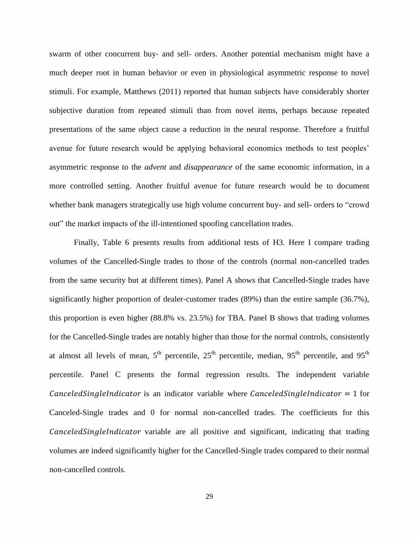
Table 3 presents the results for the test of H2 (Channel Two). Previously, Table 1 shows
that the average time span between adjacent trades 𝑇𝑅𝐴𝐶𝐸0 and 𝑇𝑅𝐴𝐶𝐸𝑛+1 is 107.6 days.
Therefore, we can treat 𝑇𝑅𝐴𝐶𝐸0 as historical cost. Table 3 Panels B1-B3 show that comparing
to historical cost 𝑇𝑅𝐴𝐶𝐸0, vendors’ fair values 𝑉𝑒𝑛𝑑𝑜𝑟𝑛 have performed quite effectively, in
that, on average, vendors’ last price 𝑉𝑒𝑛𝑑𝑜𝑟𝑛 are 83% of the times closer to the next trade
𝑇𝑅𝐴𝐶𝐸𝑛+1; they are 89.4% directionally correct; they have very high (close to 1) Rho; they have
small forecast errors and mean errors; there are no systemic patterns for bias and error. Notably,
vendors’ last price 𝑉𝑒𝑛𝑑𝑜𝑟𝑛 can bring 91.6% of variance reduction, compared to the historical
cost 𝑇𝑅𝐴𝐶𝐸0 . From Panel C1 indicates that vendors’ last price 𝑉𝑒𝑛𝑑𝑜𝑟𝑛 (red line) has
significantly reduced the inter-trade variances of historical cost (blue line) and there are no signs
of systemic biases. One unexpected result, though, from Table 3 is that there are no significant
improvements post- vs. pre- FINRA’s dissemination (Panel B2 and B3). This result is somewhat
surprising, because it is expected that FINRA’s timely dissemination of transaction data to the
public will remarkably reduce information asymmetry and increase pre-trade transparency. One
possible explanation is that market insiders such as the vendors rely on alternative more
expeditious / efficient information channels. As discussed before, vendors have direct access to
all the major trading desks; in addition, they also have access to the traders’ intention to trade
from BWIC. For most trades, dealers have to report to TRACE within 15-60 minutes of the time
of the execution. At the same time, TRACE generally disseminates trade information within 15
minutes after it receives the reported trade. So, the conservative estimate for the total timespan

25
between the execution and TRACE’s dissemination is 15-60 minutes. Although FINRA
dissemination might reduce the information asymmetry for the general public, it is most likely
that during this 15-60 minute window, market professionals including vendors, might have
already been informed through other timelier information channels.
Table 4 presents the formal regression results for the test of H2 (Channel Two). Two
different regression models are used to test H2:
𝑌 = 𝛼0 + 𝛼1 ∙ 𝑋 + 𝛼2 ∙ 𝑃𝑜𝑠𝑡𝑖,𝑡 + 𝛼3 ∙ 𝑋 × 𝑃𝑜𝑠𝑡𝑖,𝑡 + 𝐶𝑜𝑛𝑡𝑟𝑜𝑙𝑠 + 𝜖𝑖,𝑡 (2)
𝑀𝑜𝑑𝑒𝑙1: {𝑌1 = 𝑇𝑅𝐴𝐶𝐸𝑖,(𝑛+1)
𝑋1 = 𝑉𝑒𝑛𝑑𝑜𝑟𝑖,𝑛 𝑎𝑛𝑑 𝑀𝑜𝑑𝑒𝑙2: {
𝑌2 = ∆𝑇𝑅𝐴𝐶𝐸 = 𝑇𝑅𝐴𝐶𝐸𝑖,(𝑛+1) − 𝑇𝑅𝐴𝐶𝐸𝑖,0
𝑋2 = ∆𝑉𝑒𝑛𝑑𝑜𝑟 = 𝑉𝑒𝑛𝑑𝑜𝑟𝑖,𝑛 − 𝑉𝑒𝑛𝑑𝑜𝑟𝑖,0
Model 1 and Model 2 have yielded identical regression coefficients and standard errors,
except for the estimates for the constant 𝛼0. Only Model 2 results are reported in Panel A. A key
result from Panel A is the positive, significant, and close to 1 coefficients on 𝑋 = ∆𝑉𝑒𝑛𝑑𝑜𝑟.
Detailed calculations from Panel C indicate that 𝑉𝑒𝑛𝑑𝑜𝑟𝑛 can predict / account for around 85%
of the next trade price 𝑇𝑅𝐴𝐶𝐸𝑛+1 , a significant improvement over the historical cost 𝑇𝑅𝐴𝐶𝐸0.
Once again, there are no significant performance improvements after TRACE dissemination (the
interaction terms are not significant), suggesting that vendors had other timelier channels to
acquire information. Another interesting observation worth noting is that for the entire sample,
CMO, and MBS, coefficients for 𝐺𝑎𝑝 𝑏𝑡𝑤 [𝑇0, 𝑇𝑛+1] are both negative and significant,
suggesting that vendors’ accuracy forecasting the next trade price 𝑇𝑅𝐴𝐶𝐸𝑛+1 decreases with the
timespan between 𝑇𝑅𝐴𝐶𝐸0 and 𝑇𝑅𝐴𝐶𝐸𝑛+1 . This result makes intuitive sense: the longer the
timespan between [𝑇𝑅𝐴𝐶𝐸0, 𝑇𝑅𝐴𝐶𝐸𝑛+1], the less efficient and accurate the forecast.
Another important implication from Table 4 is that we can have a point estimate of the
percentage reduction of managerial discretion. Here I define managerial discretion as the
26
difference between managers’ reported value and the reference value (the most recent widely
available price):
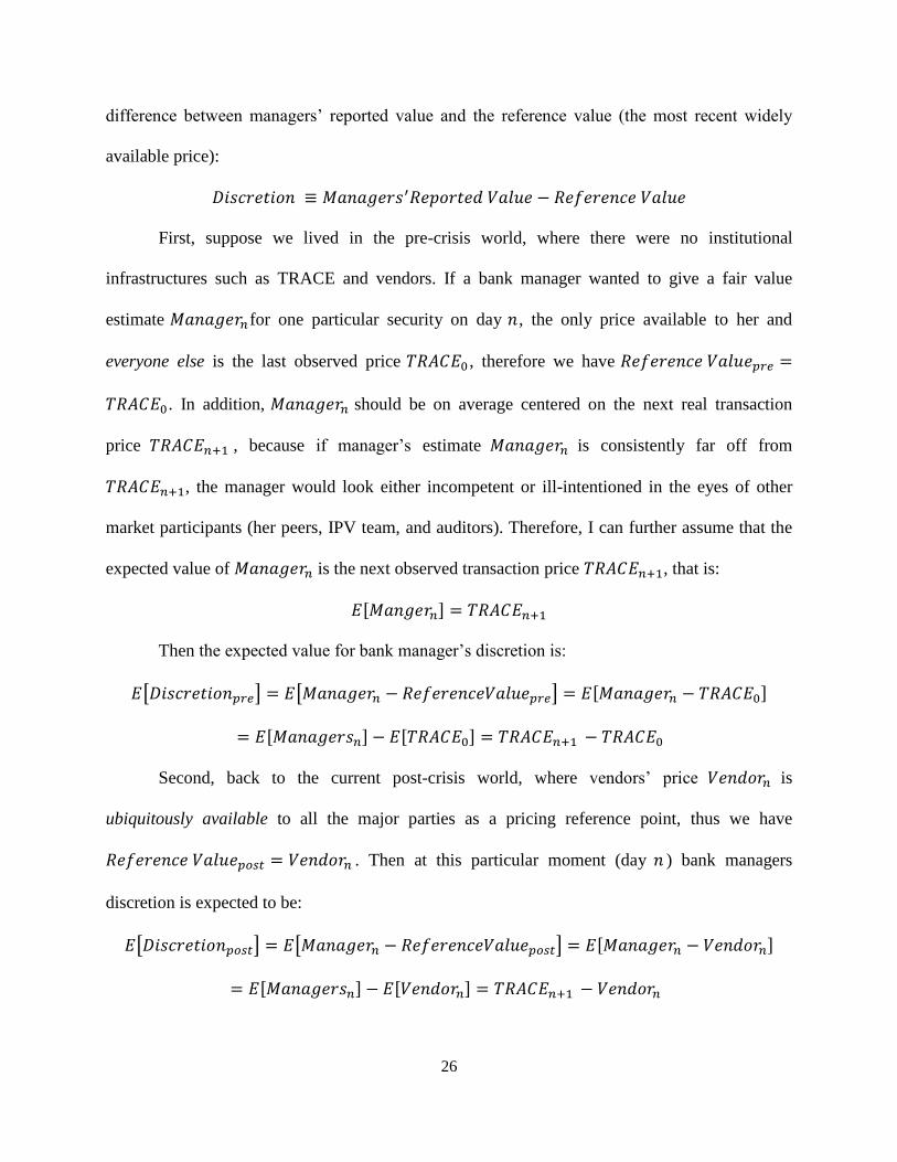
𝐷𝑖𝑠𝑐𝑟𝑒𝑡𝑖𝑜𝑛 ≡ 𝑀𝑎𝑛𝑎𝑔𝑒𝑟𝑠′𝑅𝑒𝑝𝑜𝑟𝑡𝑒𝑑 𝑉𝑎𝑙𝑢𝑒 − 𝑅𝑒𝑓𝑒𝑟𝑒𝑛𝑐𝑒 𝑉𝑎𝑙𝑢𝑒
First, suppose we lived in the pre-crisis world, where there were no institutional
infrastructures such as TRACE and vendors. If a bank manager wanted to give a fair value
estimate 𝑀𝑎𝑛𝑎𝑔𝑒𝑟𝑛for one particular security on day 𝑛 , the only price available to her and
everyone else is the last observed price 𝑇𝑅𝐴𝐶𝐸0 , therefore we have 𝑅𝑒𝑓𝑒𝑟𝑒𝑛𝑐𝑒 𝑉𝑎𝑙𝑢𝑒𝑝𝑟𝑒 =
𝑇𝑅𝐴𝐶𝐸0. In addition, 𝑀𝑎𝑛𝑎𝑔𝑒𝑟𝑛 should be on average centered on the next real transaction
price 𝑇𝑅𝐴𝐶𝐸𝑛+1 , because if manager’s estimate 𝑀𝑎𝑛𝑎𝑔𝑒𝑟𝑛 is consistently far off from
𝑇𝑅𝐴𝐶𝐸𝑛+1, the manager would look either incompetent or ill-intentioned in the eyes of other
market participants (her peers, IPV team, and auditors). Therefore, I can further assume that the
expected value of 𝑀𝑎𝑛𝑎𝑔𝑒𝑟𝑛 is the next observed transaction price 𝑇𝑅𝐴𝐶𝐸𝑛+1, that is:
𝐸[𝑀𝑎𝑛𝑔𝑒𝑟𝑛] = 𝑇𝑅𝐴𝐶𝐸𝑛+1
Then the expected value for bank manager’s discretion is:
𝐸[𝐷𝑖𝑠𝑐𝑟𝑒𝑡𝑖𝑜𝑛𝑝𝑟𝑒] = 𝐸[𝑀𝑎𝑛𝑎𝑔𝑒𝑟𝑛 − 𝑅𝑒𝑓𝑒𝑟𝑒𝑛𝑐𝑒𝑉𝑎𝑙𝑢𝑒𝑝𝑟𝑒] = 𝐸[𝑀𝑎𝑛𝑎𝑔𝑒𝑟𝑛 − 𝑇𝑅𝐴𝐶𝐸0]
= 𝐸[𝑀𝑎𝑛𝑎𝑔𝑒𝑟𝑠𝑛] − 𝐸[𝑇𝑅𝐴𝐶𝐸0] = 𝑇𝑅𝐴𝐶𝐸𝑛+1 − 𝑇𝑅𝐴𝐶𝐸0
Second, back to the current post-crisis world, where vendors’ price 𝑉𝑒𝑛𝑑𝑜𝑟𝑛 is
ubiquitously available to all the major parties as a pricing reference point, thus we have
𝑅𝑒𝑓𝑒𝑟𝑒𝑛𝑐𝑒 𝑉𝑎𝑙𝑢𝑒𝑝𝑜𝑠𝑡 = 𝑉𝑒𝑛𝑑𝑜𝑟𝑛 . Then at this particular moment (day 𝑛 ) bank managers
discretion is expected to be:
𝐸[𝐷𝑖𝑠𝑐𝑟𝑒𝑡𝑖𝑜𝑛𝑝𝑜𝑠𝑡] = 𝐸[𝑀𝑎𝑛𝑎𝑔𝑒𝑟𝑛 − 𝑅𝑒𝑓𝑒𝑟𝑒𝑛𝑐𝑒𝑉𝑎𝑙𝑢𝑒𝑝𝑜𝑠𝑡] = 𝐸[𝑀𝑎𝑛𝑎𝑔𝑒𝑟𝑛 − 𝑉𝑒𝑛𝑑𝑜𝑟𝑛]
= 𝐸[𝑀𝑎𝑛𝑎𝑔𝑒𝑟𝑠𝑛] − 𝐸[𝑉𝑒𝑛𝑑𝑜𝑟𝑛] = 𝑇𝑅𝐴𝐶𝐸𝑛+1 − 𝑉𝑒𝑛𝑑𝑜𝑟𝑛
27
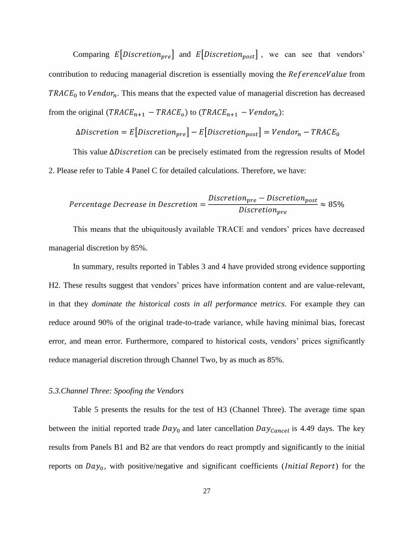
Comparing 𝐸[𝐷𝑖𝑠𝑐𝑟𝑒𝑡𝑖𝑜𝑛𝑝𝑟𝑒] and 𝐸[𝐷𝑖𝑠𝑐𝑟𝑒𝑡𝑖𝑜𝑛𝑝𝑜𝑠𝑡] , we can see that vendors’
contribution to reducing managerial discretion is essentially moving the 𝑅𝑒𝑓𝑒𝑟𝑒𝑛𝑐𝑒𝑉𝑎𝑙𝑢𝑒 from
𝑇𝑅𝐴𝐶𝐸0 to 𝑉𝑒𝑛𝑑𝑜𝑟𝑛. This means that the expected value of managerial discretion has decreased
from the original (𝑇𝑅𝐴𝐶𝐸𝑛+1 − 𝑇𝑅𝐴𝐶𝐸𝑜) to (𝑇𝑅𝐴𝐶𝐸𝑛+1 − 𝑉𝑒𝑛𝑑𝑜𝑟𝑛):
∆𝐷𝑖𝑠𝑐𝑟𝑒𝑡𝑖𝑜𝑛 = 𝐸[𝐷𝑖𝑠𝑐𝑟𝑒𝑡𝑖𝑜𝑛𝑝𝑟𝑒] − 𝐸[𝐷𝑖𝑠𝑐𝑟𝑒𝑡𝑖𝑜𝑛𝑝𝑜𝑠𝑡] = 𝑉𝑒𝑛𝑑𝑜𝑟𝑛 − 𝑇𝑅𝐴𝐶𝐸0
This value ∆𝐷𝑖𝑠𝑐𝑟𝑒𝑡𝑖𝑜𝑛 can be precisely estimated from the regression results of Model
2. Please refer to Table 4 Panel C for detailed calculations. Therefore, we have:
𝑃𝑒𝑟𝑐𝑒𝑛𝑡𝑎𝑔𝑒 𝐷𝑒𝑐𝑟𝑒𝑎𝑠𝑒 𝑖𝑛 𝐷𝑒𝑠𝑐𝑟𝑒𝑡𝑖𝑜𝑛 =𝐷𝑖𝑠𝑐𝑟𝑒𝑡𝑖𝑜𝑛𝑝𝑟𝑒 − 𝐷𝑖𝑠𝑐𝑟𝑒𝑡𝑖𝑜𝑛𝑝𝑜𝑠𝑡
𝐷𝑖𝑠𝑐𝑟𝑒𝑡𝑖𝑜𝑛𝑝𝑟𝑒≈ 85%
This means that the ubiquitously available TRACE and vendors’ prices have decreased
managerial discretion by 85%.
In summary, results reported in Tables 3 and 4 have provided strong evidence supporting
H2. These results suggest that vendors’ prices have information content and are value-relevant,
in that they dominate the historical costs in all performance metrics. For example they can
reduce around 90% of the original trade-to-trade variance, while having minimal bias, forecast
error, and mean error. Furthermore, compared to historical costs, vendors’ prices significantly
reduce managerial discretion through Channel Two, by as much as 85%.
5.3.Channel Three: Spoofing the Vendors
Table 5 presents the results for the test of H3 (Channel Three). The average time span
between the initial reported trade 𝐷𝑎𝑦0 and later cancellation 𝐷𝑎𝑦𝐶𝑎𝑛𝑐𝑒𝑙 is 4.49 days. The key
results from Panels B1 and B2 are that vendors do react promptly and significantly to the initial
reports on 𝐷𝑎𝑦0 , with positive/negative and significant coefficients (𝐼𝑛𝑖𝑡𝑖𝑎𝑙 𝑅𝑒𝑝𝑜𝑟𝑡) for the
28
positive/negative “jumps”. Vendors, however, don’t fully respond to the later cancellation on
𝐷𝑎𝑦𝐶𝑎𝑛𝑐𝑒𝑙 with non-significant coefficients (𝐿𝑎𝑡𝑒𝑟 𝐶𝑎𝑛𝑐𝑒𝑙𝑙𝑎𝑡𝑖𝑜𝑛).28
Given the results from Panel B1 and B2, I further test whether vendor prices would
eventually revert back to their original levels. Results of regressions of vendors’ prices on four
dummy variables (5 days, 10 days, 15 days, and 20 days after the cancellation) are shown in
Panels B3-4. The coefficients for 𝐷𝑎𝑦5 are slightly significant at 𝑝 = 0.1 level; they are
positive/negative for the positive/negative jumps. The coefficients for 𝐷𝑎𝑦10 and 𝐷𝑎𝑦15 are
non-significant at all; but they are still positive/negative for the positive/negative jumps. The
coefficients for 𝐷𝑎𝑦20, however, don’t even have the consistent signs for either positive or
negative jumps at all. These results indicate that vendors’ prices, on average, revert back quickly
to the original level within 10-15 days.
These results from Panel B1-B4 indicate a possibility that even the weak-form of
efficient-market hypothesis does not hold in this particular setting. Although financial
intermediaries, such as vendors, react expeditiously to the initial posted transactions, their
response to the later cancellation is asymmetrically slow and gradual. It takes more than 10 days
for the vendors to fully absorb and digest the cancellation information; and for the prices to fully
revert back to their original levels. This asymmetric reaction on 𝐷𝑎𝑦0 and 𝐷𝑎𝑦𝐶𝑎𝑛𝑐𝑒𝑙 , thus,
provides a short-term (around 10 days) predictability of the future price movements. These
results also suggest that financial intermediaries might react differently and asymmetrically to
the advent of new economic information from the disappearance of the same old information.
One potential mechanism behind this asymmetric response might be the “crowding out
effect”, in that the impact of the later cancellation is driven down or even eliminated by the
28 A positive / negative jump specifies an upward / downward adjustment on Day_0 for vendors’ prices in response to the posted
initial trades. And Initial Report and Later Cancellation are two dummy variables specifying these two event dates.
29
swarm of other concurrent buy- and sell- orders. Another potential mechanism might have a
much deeper root in human behavior or even in physiological asymmetric response to novel
stimuli. For example, Matthews (2011) reported that human subjects have considerably shorter
subjective duration from repeated stimuli than from novel items, perhaps because repeated
presentations of the same object cause a reduction in the neural response. Therefore a fruitful
avenue for future research would be applying behavioral economics methods to test peoples’
asymmetric response to the advent and disappearance of the same economic information, in a
more controlled setting. Another fruitful avenue for future research would be to document
whether bank managers strategically use high volume concurrent buy- and sell- orders to “crowd
out” the market impacts of the ill-intentioned spoofing cancellation trades.
Finally, Table 6 presents results from additional tests of H3. Here I compare trading
volumes of the Cancelled-Single trades to those of the controls (normal non-cancelled trades
from the same security but at different times). Panel A shows that Cancelled-Single trades have
significantly higher proportion of dealer-customer trades (89%) than the entire sample (36.7%),
this proportion is even higher (88.8% vs. 23.5%) for TBA. Panel B shows that trading volumes
for the Cancelled-Single trades are notably higher than those for the normal controls, consistently
at almost all levels of mean, 5th
percentile, 25th
percentile, median, 95th
percentile, and 95th
percentile. Panel C presents the formal regression results. The independent variable
𝐶𝑎𝑛𝑐𝑒𝑙𝑒𝑑𝑆𝑖𝑛𝑔𝑙𝑒𝐼𝑛𝑑𝑖𝑐𝑎𝑡𝑜𝑟 is an indicator variable where 𝐶𝑎𝑛𝑐𝑒𝑙𝑒𝑑𝑆𝑖𝑛𝑔𝑙𝑒𝐼𝑛𝑑𝑖𝑐𝑎𝑡𝑜𝑟 = 1 for
Canceled-Single trades and 0 for normal non-cancelled trades. The coefficients for this
𝐶𝑎𝑛𝑐𝑒𝑙𝑒𝑑𝑆𝑖𝑛𝑔𝑙𝑒𝐼𝑛𝑑𝑖𝑐𝑎𝑡𝑜𝑟 variable are all positive and significant, indicating that trading
volumes are indeed significantly higher for the Cancelled-Single trades compared to their normal
non-cancelled controls.

30
In summary, Cancelled-Single trades have significantly higher trading volumes and
consist of pre-dominantly dealer-customer trades. These two pieces of evidence collectively
indicate a possibility that these Cancelled-Single trades might not be the result of simple input
errors, in that random errors would have caused equally higher or lower erroneous trading
volume; they would also have happened equally in dealer-customer or inter-dealer trades.
Instead, this evidence suggests another possibility: bank managers might use these spoofing
Cancelled-Single trades to manipulate vendors’ fair values. As discussed before, FINRA
mandates that in dealer-customer trades, only the dealer need to report to TRACE, while in an
inter-dealer trade, both dealers need to report to TRACE. Therefore, manipulation in inter-dealer
trades requires a significantly higher level of collusion. In the meantime, higher than usual
trading volumes are more sensational and could have a more notable impact on vendors’ prices.
I have to emphasize three points here. First, there is no definitive proof that bank
managers use Cancelled-Single trades to spoof the market and manipulate fair value prices. The
definitive proof would need to substantiate that the intent for the initial posted trades is not to
execute, but to cancel.29
Though specific intent is exceedingly difficult to establish,30
Tables 5
and 6 do provide solid evidence that financial intermediaries respond asymmetrically to the
advent and later disappearance of the same economic information; and that trading volumes and
dealer-customer proportion are significantly and consistently higher in Cancelled-Single trades.
This evidence indicates that Cancelled-Single trade might be one of the potential channels that
bank managers could use to spoof vendors’ fair value prices. This lack of definitive proof
naturally leads to unresolved issues and directions for future research. For example, a fruitful
29 For example, in a 2012 report Finansinspektionen (FI), the Swedish Financial Supervisory Authority defined spoofing/layering
as "a strategy of placing orders that is intended to manipulate the price of an instrument, for example through a combination
of buy and sell orders." 30 Kluchenek & Kahn, supra note 4, at 129 n.48 (citing Jerry W. Markham, Manipulation of Commodity Futures Prices—The
Unprosecutable Crime, YALE J. ON REG. 281, 356–57 (1991)).

31
avenue for future research would be to provide further evidence on the dynamics between banks
managers and vendors. For example, do Cancelled-Single trades occur more frequently during
stress times due to credit shock, interest shock, high volatility, etc.? Another fruitful avenue for
future research would be to incorporate commercially available BWIC or Bloomberg messages
posted by traders to further test whether they strategically use these messages to artificially spoof
market sentiment and manipulate market expectations.
Second, the scope of the Cancelled-Single trades is very limited. Table 5 Panel A2 shows
that out of the 16,020,744 total transactions, there are only 4,144 Cancelled-Single trades, with
50 from ABS, 535 from CMO, 3,399 from MBS, and 160 from TBA. These Cancelled-Single
trades are quite rare, and account for only 0.02% of the total trading volume of the entire sample
and 0.28% of the daily trading volume. Therefore, the impact of Cancelled-Single trade on the
overall market is immaterial, if not totally negligible. In addition, the timespan for potential
Cancelled-Single trades is also very limited. The artificially inflated (deflated) fair value prices
and associated market sentiment of over-optimism (over-pessimism) from spoofing trades are
short-lived. Results from Table 5 Panel B indicate that market sentiments represented by
vendors’ prices are only slightly higher than the original level on the 5th
day, and completely
revert back to the original level within 10-15 days. Furthermore, the bank manager who initiated
the original Cancelled-Single trade is fully aware that other traders may also recognize the over-
optimism (over-pessimism) through access to vendors’ pricing feeds. Therefore, the real window
to take advantage of the Cancelled-Single trades is most likely even shorter.
Third, although the Cancelled-Single trades might seem to be immaterial to the overall
market, they might have consequential impacts on individual bank trader’ performance. This
spoofing is at the very micro individual trader or portfolio manager level, not at the firm level.

32
The unrealized gains and losses through potential spoofing are recognized in other
comprehensive income (OCI). The unrealized gains and losses are recognized in earnings only
when they are realized through real transactions (Barth et al. 2014). Thus, the spoofing and fair
value manipulation will have no direct impacts on a firm’s earnings or a CEO’s performance per
se. However, unrealized gains and losses are still relevant to this study due to three reasons. First,
prior studies find that other comprehensive income is value relevant, particularly the unrealized
securities gains and losses component (Dhaliwal et al. 1999; Biddle and Choi 2006; Chambers et
al. 2007; Bamber et al. 2010). Second, the unrealized gains and losses through potential spoofing
will definitely have an effect on an individual trader or portfolio manager’s portfolio valuation
and associate performances/bonus. In fact, portfolio managers’ manipulation of vendors’ fair
value prices to their advantages is not uncommon. The most well-known case is PIMCO’s odd-
lot discount manipulation.31
Third, although the unrealized gains or losses themselves might not
affect firm’s earning, banks (at firm level) might still use subsequent real transactions to reap the
benefits of the artificially created over-pessimism or over-optimism from spoofing.32
Therefore,
another fruitful avenue for future research would be to document whether banks, following the
initial Cancelled-Single trades, use subsequent separate real transactions to cash in (and
recognize in earnings) these unrealized gains and losses induced by spoofing.
In summary, results reported in Tables 5 and 6 have provided strong evidence supporting
H3. Prior evidence supporting H1 and H2 suggests that the new institutional developments have
31 PIMCO agreed to pay disgorgement of fees totaling $1,331,628.74 plus interest of $198,179.04 and a penalty of $18.3 million
to SEC. “Odd lots”, irregularly sized bundles of bonds, are generally traded at a discount compared to full-price “round lots”.
On March 9, 2012, PIMCO purchased an MBS odd lot at $64.9999 with a current face of $0.2 million. PIMCO then valued
the position at a third-party pricing vendor’s institutional round lot mark of $82.74585 (a 27% increase). This manipulation
alone increased PIMCO fund’s NAV by as much as 31 cents 32 According to the July 2013 CFTC’s milestone case against spoofing, spoofers placed a "relatively small order to sell futures
that they did want to execute, which they quickly followed with several large buy orders at successively higher prices that
they intended to cancel”. By placing the large buy orders, spoofers “sought to give the market the impression that there was
significant buying interest, which suggested that prices would soon rise, raising the likelihood that other market participants
would buy from the small order” spoofers were then offering to sell.

33
put significant constraints on managerial discretion in Channels One and Two. Therefore, bank
managers must find an alternative channel to manipulate fair values. Results from Tables 5 and 6
suggest that bank managers could engage in more spoofing-transaction based fair value
manipulation through Channel Three.
6. Conclusion
In this study, I find that banks predominantly apply vendors’ feeds to generate financial
statements. In addition, external auditors also predominantly rely on (different) vendors’ pricing
feeds and expertise to verify and challenge banks’ fair values. I also find that vendors’ evaluated
prices dominate the historical costs in all performance metrics and can be a more accurate,
objective, and reliable proxy for fair value than historical cost. In addition, vendors’ prices are
value-relevant in that they can account for 90% of the price variances between trades and put an
upper bound on managerial discretion, sometimes to only 15% of the original level. Lastly, there
are only limited channels through which managers can manipulate fair values. Recent
institutional developments have put significant constraints on managerial discretion through
Channel One and Two. However, there are signs that bank managers could manipulate fair
values through Channel Three. Taken together, my research suggests that recent institutional
changes after 2010 have established permanent constraints on managerial discretion over fair
values, which might be more objective (or less subjective), less costly to implement, and more
convenient for auditors to verify and challenge, than the literature previously reported.
Moreover, I emphasize the following. First, the purpose of this study is not to take sides
in the fair value debate; rather I strive to document the recent institutional changes and novel
infrastructure developments essential to both sides of the debate. Second, the main focus of this
study is not to compare managerial discretion in the pre- and post- TRACE/vendors periods,

34
which would be an effective approach only in the absence of the understanding of the underlying
causal mechanism. Rather I try to assess vendor performance by comparing vendor prices
directly to the historical costs in the post- period. This choice is, firstly, due to data availability
(i.e. TRACE only started collecting SCP transaction data on May 16, 2011). Secondly, prior
discussions on field research and causal inference suggest that the first order effects and the
causal mechanism come directly from vendors’ effective performance (i.e. vendors’ prices can
reliably and accurately predict next trade prices). Therefore, once the field research has
pinpointed the underlying causal mechanism, comparing the pre- and post- periods, a joint test
for macro-level aggregated association itself, can only provide corroborating and additional
evidence (Gow et. al. 2016). At the same time, some recent studies try to provide this
corroborating evidence by investigating the effect of vendors’ prices on management’s real
transaction based earning and capital management, for example (Liu 2017).
Finally, I wish to remark on vendors’ role and fair value accounting from a broader
perspective. A common thread that I weave throughout this study is how vendors’ prices affect
managerial discretion and the potential ways they can manipulate fair values. From a narrower
and shorter-term perspective, vendors’ evaluated prices do seem to put significant constraints on
managerial discretion. However, I should also discuss several critical caveats / negative
consequences and guard against falling into a false sense of security and invulnerability from
vendors’ prices. It is far too early to celebrate the triumph of fair value accounting for the
following four reasons.
First of all, the next trade price 𝑇𝑅𝐴𝐶𝐸𝑛+1 might not be entirely exogenous to vendors’
prices at all. Due to vendors’ increasing clout and ubiquitous availability of their evaluated prices,
both the buy- and sell- side traders might use vendors’ last price 𝑉𝑒𝑛𝑑𝑜𝑟𝑛 as a reference point

35
when they negotiate the next trade. Therefore, it might not be a total surprise after all that
vendors’ price 𝑉𝑒𝑛𝑑𝑜𝑟𝑛 can passively account for 85% of the inter-trade price movement,
because they can, in fact, actively induce or even “produce” the next trade price 𝑇𝑅𝐴𝐶𝐸𝑛+1.
Second, as discussed previously, the vendors’ job is not to find securities’ intrinsic values; rather
their primary concern is to pass on all relevant information in the form of a single price, at which
“the next transaction is mostly likely to occur for this particular moment.” Therefore, vendors
will keep efficiently passing on irrationally exuberant market orders even if the security is
evidently overvalued. Third, vendors’ price identification for a non-traded security mainly relies
on cross-references to transactions of similar securities through a relational network of implied
valuation inputs. In addition to this relational network, the ubiquitous availability of vendors’
prices has made the entire financial system more tightly connected. While increased
interdependence and cross-reference might decrease the idiosyncratic valuation risks for
individual securities, they can significantly increase the systematic risks for the entire financial
system, because the very foundation of the entire relational network might be dubious and shaky.
Finally, recent institutional changes, together with the rapid development of information
technology, have made vendors’ fair value “production” an automatic, standardized, and even
mechanical process built on an information assembly line. This hard-wired and mechanical
process has made localized news and sentiments proliferate more efficiently and ubiquitously
through the financial system. More importantly, it might create self-reinforcing feedback loops
that amplify originally localized optimistic/pessimistic sentiments and opinions, thus
exacerbating system instability. For instance, vendors’ prompt markdown in response to a
random fire sale at a reginal bank might reverberate throughout the entire financial system and
ultimately trigger systemic collapse.

36
FIGURE 1 Overall Picture of the Internal and External Control Mechanisms and Constraints of Bank Managers’ Discretion
Virtually all trades must be reported to TRACE, no secretes
VendorsBack-office
Platform
General
Ledger
Financial
Statements
Bank Managers
Independent Price
Verification (IPV)
Valuation Committee
Governance/Oversight
Issue
Challenge
Report to
Brokers/
Dealers
External
Auditor
Issue
Challenge
TRACE
FINRA
Vendors
Opening up the “Black Box”
Daily Management
①
②
③
④ ⑤ ⑥
②
⑦
⑧
⑨
⑩
⑪
Audit
Audit
Direct Contact

37
Figure 1 presents the schematic illustration of the components if I open up the black box. The dotted square represents bank’s boundary. Red solid
arrowed lines (① to ⑥) represent the information flow from bank managers ultimately to bank’s financial statements. Green dotted lines (⑦ to
⑪) represent interactions (challenge, verification, etc.) between these components. Green solid lines represent the internal oversight and control
within the bank (valuation committee, IPV team, and bank managers).
We start with bank manager box in the middle. According to FINRA’s rules, virtually all trades of SCPs between bank managers and
broker/dealers (①) have to be reported (mostly within 15-60 minutes of execution) to TRACE (②). Bank managers can’t engage in
secrete trades.
Third-party pricing vendors gather transaction information either directly from broker/dealer, or from TRACE (③), BWIC, and all other
relevant channels (⑧). Vendors then generate daily fair value prices and deliver them through batch files to banks’ back-office platform
via secure FTP (④).
After quality check, all the fair value prices are entered into banks general ledger (⑤), and ultimately flow to the financial statements
(⑥). Bank managers don’t have direct inputs to the general ledger. There are only three possible ways for bank managers to manipulate
fair values: 1) cherry pick among vendors; 2) convince the committee and IPV team to issue challenges, thus change the general ledger
accounting numbers; and 3) manipulating vendors’ prices through spoofing transactions.
External auditors also predominantly rely on different vendors’ prices (⑦) to challenge bank managers’ fair values (⑩) and audit their
financial statements (⑪).
Bank’s Independent Price Verification (IPV) team manages the daily operation of the fair value process. It is also the IPV team (not the
bank managers) who will decide whether to issue challenge back to the vendors (⑨).
In addition, most of banks that I interviewed have policy / mechanisms against fraud transactions:
“Best Execution”, in which traders must have at least 3 price quotes from at least 3 different dealers in order to make the transaction.
Traders must choose the best prices among the 3 price quotes.33
Many banks have set up policies/rules against “short-term round-trip” transactions, such as repo 105. In addition, banks also have
“Wash sale” rules, which specify that the span of round-trip transactions has to be longer than 60 days.
33 In my field research, I personally witnessed a case in which one manager did not like a huge mark-down from the vendor. The trader got a favorite price quote from his
“buddy” from another bank, and then issued a challenge request to the IPV team. But the IPV team denied the challenge request.

38
T A B L E 1
Summary and Descriptive Statistics
Panel A: TRACE Data Cleaning Procedure
No. of Transactions Reduction Percentage
Original TRACE Data Delivery 25,185,925
Delete Cancellations, Corrections, and Reversals 24,188,097 3.96%
Delete the NEW Cancellations 23,582,667 6.37%
Delete interdealer transactions (one of the sides BUY) 16,020,744 36.39%
Panel B: Descriptive Statistics of TRACE Data after the Cleaning Procedure
Sample
Start
TRACE
Dissemination
Sample
End
Total No. of
Transactions
Percentage of
Transactions
Unique
CUSIP
Percentage of
CUSIP
Security Type
ABS 5/16/2011 6/1/2015 12/31/2015 292,646 1.8% 4,709 0.9%
CMO 5/16/2011 3/20/2017 12/31/2015 2,824,963 17.6% 114,328 21.8%
MBS 5/16/2011 7/22/2013 12/31/2015 4,025,440 25.1% 401,931 76.5%
TBA 5/16/2011 11/12/2012 12/31/2015 8,877,695 55.4% 4,206 0.8%
Entire Sample 16,020,744 100.0% 525,174 100.0%
Panel C: Descriptive Statistics of Weighted-Average-Life, Liquidity, and Trading Activity)
WAL
(year)
Liquidity Score
(1-5)
No. of Trade
per CUSIP
Unique Trading
Days per
CUSIPMean Mean Mean Mean Mean Median
Security Type
ABS 4.34 2.91 12.85 6.94 79.76 51.42
CMO 4.87 3.33 7.64 4.38 106.54 79.47
MBS 4.19 3.75 4.44 3.21 108.17 75.00
TBA . 4.31 9.11 5.75 107.65 78.85
Entire Sample 4.27 3.70 5.17 3.49 107.60 75.90
Timespan between Adjacent
Trading Days
Panel D: TRACE Reporting Timeframes for different Security Types (Effective December 01, 2015)
Reporting Times
Security Type
Corporate Bond Within 15 minutes of time of execution
Agency Debt Security Within 15 minutes of time of execution
Agency Pass‐Through MBS Traded TBA for Good Delivery Within 15 minutes of time of execution
Agency Pass‐Through MBS Traded TBA not for Good Delivery Within 60 minutes of time of execution
Specified Pool Transactions & SBA Backed ABS Transactions Within 60 minutes of time of execution
Asset‐Backed Securities Within 15 minutes of time of execution
All other Securitized Products: CDO, CLO, CBO Same day during TRACE business hours
CMOs/REMICs Same day during TRACE system hours

39
The original TRACE dataset has 25,185,925 rows and 36 data fields (including CUSIP, price, trading
volume, trade status, trade type, contra-party indicator, etc.). There are five possible trade status, regular
trade (T), cancelled trade (X), cancelled correction (C), new correction (R), and reversal (Y). In this
study, I mainly focus on the first two: regular trades (T) and cancelled trades (C).
There are two possible transaction types: principal and agency transactions. According to Section 206(3)
of the Investment Advisers Act, a principal transaction is a situation where a registered investment
advisor “acts as a principal for its own account and knowingly sells securities to, or buys securities from,
a client”; while an agency transaction occurs when a registered investment advisor “arranges a trade
between different advisory clients”.
Contra-party indicator specifies two different types of trades in TRACE data: a dealer-customer trade is
between a dealer and a customer (“Contra-Party” indicator = Customer); an inter-dealer trade is between
two dealers (“Contra-Party” indicator = Dealer). According to FINRA’s rule, in trades between a dealer
and a customer, only the dealer need to report to TRACE, while in an inter-dealer trade, both dealers need
to report to TRACE. Thus we expect to see significantly higher proportion of dealer-customer trades in
the Cancelled-Single trade sample.
Panel A reports the TRACE data cleaning procedure. I follow the cleaning filter algorithms outlined in
(Nick-Nielsen 2014) and (Rossi 2014), both of which drop around 35% of all the raw transactions. Panel
A reports a similar total filtering rate of 36.39%.
Panel B reports the descriptive statistics of TRACE data after the cleaning procedure. Though TRACE
has been collecting all transaction data since May 16, 2011, FINRA has been disseminating this
information to the market in different phases (staged dissemination).
In Panel C, WAL stands for Weighted Average Life. The most interesting results are that the average
number of trades for each security is 5.17; and the average number of days between adjacent observed
transactions on TRACE is 107.6 calendar days (more than 3 months).
Panel D reports the TRACE reporting timeframes for different security types (effective December 01,
2015). Most of the SCP transactions have to be reported to TRACE within 60 minutes of the time of the
execution.

40
T A B L E 2
Channel One – Strategic Vendor Selection
Panel A: Regression Results
Model:
𝐹𝑖𝑟𝑠𝑡𝑉𝑒𝑛𝑑𝑜𝑟𝑃𝑟𝑖𝑐𝑒𝑖,𝑡 = 𝛼0 + 𝛼1 ∙ 𝑆𝑒𝑐𝑜𝑛𝑑𝑉𝑒𝑛𝑑𝑜𝑟𝑃𝑟𝑖𝑐𝑒𝑖,𝑡 + 𝜖𝑖,𝑡
Panel A presents regression results comparing pricing feeds from two different vendors.
𝐹𝑖𝑟𝑠𝑡𝑉𝑒𝑛𝑑𝑜𝑟𝑃𝑟𝑖𝑐𝑒 denotes the pricing feed from Vendor 1, 𝑆𝑒𝑐𝑜𝑛𝑑𝑉𝑒𝑛𝑑𝑜𝑟𝑃𝑟𝑖𝑐𝑒 denotes the pricing
feed from Vendor 2. Panel A indicates that the pricing feeds from two different vendors are quite similar
on average, with high (close to 1) coefficient 𝛼1 (𝛼1 ≈ 1) and high (close to 1) adjusted R-square (𝑅2 ≈1). In addition, the joint F-tests for 𝛼0 = 0 𝑎𝑛𝑑 𝛼1 = 1 are all significant at the 𝑝 < 0.01 levels. Results
from Panel A imply that the pricing feeds from two different vendors are on average very similar.
Panel B shows the histograms for the differences of two pricing feeds. The red and blue lines represent
kernel density curves and normal curves, respectively. The kernel density curves are symmetrical and
much narrower than the normal curves, showing no signs of systematic biases. More importantly, the
kernel density curves are “thin-tailed”, compared to corresponding normal curves.
Panel C presents the results for formal normality test. It is clear that the distributions for the differences
are not normal, primarily due to the low variance and high kurtosis (any kurtosis higher than 3 means
thin-tailed distribution). This implies once again that the pricing differences are thin-tailed and that
extreme pricing differences between two vendors are unlikely to occur compared to normal distributions.
(1) (2) (3) (4) (5)
Entire Sample ABS CMO MBS TBA
Vendor2 0.951*** 0.965*** 0.932*** 0.952*** 0.942***
(3.91) (5.94) (3.62) (4.93) (4.18)
Observations 952,055 11,368 207,036 733,648 1,452
Adj R-squared 0.95802 0.97651 0.93183 0.92662 0.9242
CUSIP FE Yes Yes Yes Yes Yes
Date FE Yes Yes Yes Yes Yes
Joint F-test on 5.84*** 5.93*** 4.37*** 5.52*** 5.24***
α0=0 AND α1=1
Clustered t-statistics by both date and CUSIP in parentheses (continued)
*** p<0.01, ** p<0.05, * p<0.1

41
Panel B: Histograms of Price Differences of Pricing Feeds from Two Different Vendors
𝑃𝑟𝑖𝑐𝑒𝐷𝑖𝑓𝑓𝑒𝑟𝑒𝑛𝑐𝑒𝑠𝑖𝑡 = 𝐹𝑖𝑟𝑠𝑡𝑉𝑒𝑛𝑑𝑜𝑟𝑃𝑟𝑖𝑐𝑒𝑖,𝑡 − 𝑆𝑒𝑐𝑜𝑛𝑑𝑉𝑒𝑛𝑑𝑜𝑟𝑃𝑟𝑖𝑐𝑒𝑖,𝑡
(Continued)
Panel C. Normality Test Results
Mean Variance Skewness KurtosisKolmogorov-
Smirnov
Cramer-
von Mises
Anderson-
Darling
Security Type
ABS 0.00 0.00 1.38 3.49 <0.010 <0.005 <0.005
CMO 0.00 0.00 1.39 6.47 <0.010 <0.005 <0.005
MBS 0.00 0.00 -0.85 15.22 <0.010 <0.005 <0.005
TBA 0.00 0.00 0.10 5.03 <0.010 <0.005 <0.005
Entire Sample 0.00 0.00 -0.46 14.38 <0.010 <0.005 <0.005
Standard Normal 0.00 1.00 0.00 3.00

42
T A B L E 3
Channel Two - Vendor Effective Performance
(Descriptive Results)
Panel A: Definitions and Illustration of Commonly Used Performance Metrics
Definition
Time Point
0: 𝐷𝑎𝑦 0 -- Last Observed Trade on Day 0 Last TRACE Reported Transaction
1:Days between [𝐷𝑎𝑦 0, 𝐷𝑎𝑦 𝑛] Might be 3 months in between
2:𝐷𝑎𝑦 𝑛 -- Vendor’s last price on Day 𝑛 before Next Trade Vendor Evaluated Daily Price on Day 𝑛
3: 𝐷𝑎𝑦 (𝑛 + 1) -- Next Observed Trade on Day (𝑛 + 1) Next TRACE Reported Transaction
Regression Analogy: 𝑦 = 𝜅 ∙ 𝑥 + 𝜖
Calculation Formula Regression Analogy
Variable Definition
𝑦 = 𝑟𝑒𝑡𝑢𝑟𝑛(3,0), 𝑁𝑒𝑥𝑡𝑇𝑅𝐴𝐶𝐸 𝐿𝑎𝑠𝑡𝑇𝑅𝐴𝐶𝐸⁄ − 1 = 𝑇𝑛+1 𝑇0⁄ − 1 Dependent Variable
𝑥 = 𝑟𝑒𝑡𝑢𝑟𝑛(2,0), 𝑉𝑒𝑛𝑑𝑜𝑟𝐿𝑎𝑠𝑡𝑃𝑟𝑖𝑐𝑒 𝐿𝑎𝑠𝑡𝑇𝑅𝐴𝐶𝐸⁄ − 1 = 𝑣𝑛 𝑇0⁄ − 1 Independent Variable
𝜖 = 𝑟𝑒𝑡𝑢𝑟𝑛(3,2), 𝑁𝑒𝑥𝑡𝑇𝑅𝐴𝐶𝐸 𝑉𝑒𝑛𝑑𝑜𝑟𝐿𝑎𝑠𝑡𝑃𝑟𝑖𝑐𝑒⁄ − 1 = 𝑇𝑛+1 𝑣𝑛⁄ − 1 Residual
Calculation Formula
Performance Metrics
Rho(𝜌): 𝑐𝑜𝑟𝑟𝑒𝑙𝑎𝑡𝑖𝑜𝑛(𝑥, 𝑦), 𝜌 = 𝑟𝑒𝑔𝑟𝑒𝑠𝑠𝑖𝑜𝑛 𝑐𝑜𝑒𝑓𝑓𝑖𝑐𝑖𝑒𝑛𝑡 𝜅 × 𝜎𝑥 𝜎𝑦⁄ ,
Days_Closer: 𝐻𝑜𝑤 𝑚𝑎𝑛𝑦 𝑡𝑖𝑚𝑒𝑠 |𝜖| < |𝑦|,
Directional_Correct: 𝐻𝑜𝑤 𝑚𝑎𝑛𝑦 𝑡𝑖𝑚𝑒𝑠 𝑠𝑖𝑔𝑛(𝑦) = 𝑠𝑖𝑔𝑛(𝑥),
Forecast_Error: 𝑚𝑒𝑎𝑛(|𝜖|)/𝑚𝑒𝑎𝑛(|𝑦|),
Model Bias: 𝑐𝑜𝑟𝑟𝑒𝑙𝑎𝑡𝑖𝑜𝑛(𝑥, 𝜖), 𝑎 𝑚𝑒𝑎𝑠𝑢𝑟𝑒 𝑜𝑓 𝑎𝑟𝑏𝑖𝑡𝑟𝑎𝑔𝑒 𝑜𝑝𝑝𝑜𝑟𝑡𝑢𝑛𝑖𝑡𝑖𝑒𝑠,
Variance_Reduction: 1 – 𝑣𝑎𝑟𝑖𝑎𝑛𝑐𝑒(𝜖)/𝑣𝑎𝑟𝑖𝑎𝑛𝑐𝑒(𝑦), 𝑟𝑒𝑔𝑟𝑒𝑠𝑠𝑖𝑜𝑛 𝑅 𝑠𝑞𝑎𝑟𝑒,
Mean_Error: 𝑚𝑒𝑎𝑛(𝜖).
Last
Trade
TRACE
Vendor
Price
02 3
Time
Vendor
Price
Vendor
Price
…………
Vendor
PriceNext
Trade
TRACE
There could be 3 months between two adjacent trades;
vendors fill in the daily prices in between 1
Historical
Costs
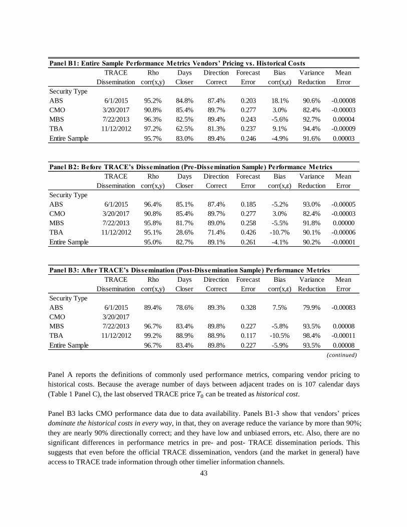
43
Panel A reports the definitions of commonly used performance metrics, comparing vendor pricing to
historical costs. Because the average number of days between adjacent trades on is 107 calendar days
(Table 1 Panel C), the last observed TRACE price 𝑇0 can be treated as historical cost.
Panel B3 lacks CMO performance data due to data availability. Panels B1-3 show that vendors’ prices
dominate the historical costs in every way, in that, they on average reduce the variance by more than 90%;
they are nearly 90% directionally correct; and they have low and unbiased errors, etc. Also, there are no
significant differences in performance metrics in pre- and post- TRACE dissemination periods. This
suggests that even before the official TRACE dissemination, vendors (and the market in general) have
access to TRACE trade information through other timelier information channels.
Panel B1: Entire Sample Performance Metrics Vendors’ Pricing vs. Historical Costs
TRACE
Dissemination
Rho
corr(x,y)
Days
Closer
Direction
Correct
Forecast
Error
Bias
corr(x,ɛ)
Variance
Reduction
Mean
Error
Security Type
ABS 6/1/2015 95.2% 84.8% 87.4% 0.203 18.1% 90.6% -0.00008
CMO 3/20/2017 90.8% 85.4% 89.7% 0.277 3.0% 82.4% -0.00003
MBS 7/22/2013 96.3% 82.5% 89.4% 0.243 -5.6% 92.7% 0.00004
TBA 11/12/2012 97.2% 62.5% 81.3% 0.237 9.1% 94.4% -0.00009
Entire Sample 95.7% 83.0% 89.4% 0.246 -4.9% 91.6% 0.00003
Panel B2: Before TRACE’s Dissemination (Pre-Dissemination Sample) Performance Metrics
TRACE
Dissemination
Rho
corr(x,y)
Days
Closer
Direction
Correct
Forecast
Error
Bias
corr(x,ɛ)
Variance
Reduction
Mean
Error
Security Type
ABS 6/1/2015 96.4% 85.1% 87.4% 0.185 -5.2% 93.0% -0.00005
CMO 3/20/2017 90.8% 85.4% 89.7% 0.277 3.0% 82.4% -0.00003
MBS 7/22/2013 95.8% 81.7% 89.0% 0.258 -5.5% 91.8% 0.00000
TBA 11/12/2012 95.1% 28.6% 71.4% 0.426 -10.7% 90.1% -0.00006
Entire Sample 95.0% 82.7% 89.1% 0.261 -4.1% 90.2% -0.00001
Panel B3: After TRACE’s Dissemination (Post-Dissemination Sample) Performance Metrics
TRACE
Dissemination
Rho
corr(x,y)
Days
Closer
Direction
Correct
Forecast
Error
Bias
corr(x,ɛ)
Variance
Reduction
Mean
Error
Security Type
ABS 6/1/2015 89.4% 78.6% 89.3% 0.328 7.5% 79.9% -0.00083
CMO 3/20/2017
MBS 7/22/2013 96.7% 83.4% 89.8% 0.227 -5.8% 93.5% 0.00008
TBA 11/12/2012 99.2% 88.9% 88.9% 0.117 -10.5% 98.4% -0.00011
Entire Sample 96.7% 83.4% 89.8% 0.227 -5.9% 93.5% 0.00008
(continued)

44
Panel C1: Radar Chart Representations of Variance Reduction by Vendors’ Pricing Feeds
(Continued)

45
Panel C2: Representations of Variance Reduction by Vendors’ Pricing Feeds vs. Historical Costs
The intuition behind the definitions of 𝑦, 𝑥, 𝑎𝑛𝑑 𝜖 in Panel A and C2 is that we can treat the performance
comparison between vendor prices and historical costs as a regression model:
𝑦 = 𝜅 ∙ 𝑥 + 𝜖 (∗)
𝑦 = 𝑇𝑛+1 𝑇0⁄ − 1 represents the original price change [𝑇0, 𝑇𝑛+1 ] without vendor prices 𝑣𝑛;
𝑥 = 𝑣𝑛 𝑇0⁄ − 1 represents vendor’s contribution, that is, the part of the price movement
[𝑣𝑛, 𝑇𝑛+1 ] that can be explained or accounted for by vendor price 𝑣𝑛;
𝜖 = 𝑇𝑛+1 𝑣𝑛⁄ − 1 represents regression residual, which cannot be explained by vendor price 𝑣𝑛.
In this regression model, 𝜅 is the regression coefficient 𝜅 = 𝜌 × 𝜎𝑦 𝜎𝑥⁄ , where 𝜌 = 𝑐𝑜𝑟𝑟𝑒𝑙𝑎𝑡𝑖𝑜𝑛(𝑦, 𝑥);
Variance_Reduction is nothing but the regression R-squared. In a perfect world, where vendors are doing
a prefect job, their price 𝑣𝑛 should be “spot-on”, landing on the moving target of 𝑇𝑛+1, that is, 𝑣𝑛 = 𝑇𝑛+1.
Thus, we should have 𝜅 = 1 and 𝜖 = 0. In a less perfect world, we should have 𝜅 ≠ 1 and 𝜖 ≠ 0.
In Panel C1, blue lines represent the variance of 𝑦 = 𝑇𝑛+1 𝑇0⁄ − 1 , that is, variance of the original
regression dependent variable 𝑦 , without the contribution from the independent variable 𝑥 ; red lines
represent variance of 𝜖 = 𝑇𝑛+1 𝑣𝑛⁄ − 1 , that is, variance of the regression residual, with the contribution
from the independent variable 𝑥. The comparison of blue lines vs. red lines in Panel C1 can be interpreted
as variance without vs. with the contribution of 𝑥 from vendors.
Once again, Panel C1 shows that vendors’ prices dominate the historical costs in every way, in that, they
significantly reduce the variance between two observed TRACE prices. There are no obvious patterns or
systemic biases of vendors’ pricing feeds.
Last
Trade
TRACE
Next
Trade
TRACE
Vendor
PriceVendor
Price
Vendor
Price
…………
Vendor
Price
Average of 3 months between adjacent trades
Vendors fill in the daily prices in between
Time
Price
=100%
Historical
Costs
Quarter EndUpper Bound

46
T A B L E 4
Channel Two - Vendor Effective Performance
(Regression Results)
Panel A: Regression Results
𝑌 = 𝛼0 + 𝛼1 ∙ 𝑋 + 𝛼2 ∙ 𝑃𝑜𝑠𝑡𝑖,𝑡 + 𝛼3 ∙ 𝑋 × 𝑃𝑜𝑠𝑡𝑖,𝑡 + 𝐶𝑜𝑛𝑡𝑟𝑜𝑙𝑠 + 𝜖𝑖,𝑡
𝑀𝑜𝑑𝑒𝑙1: {𝑌1 = 𝑇𝑅𝐴𝐶𝐸𝑖,(𝑛+1)
𝑋1 = 𝑉𝑒𝑛𝑑𝑜𝑟𝑖,𝑛 𝑎𝑛𝑑 𝑀𝑜𝑑𝑒𝑙2: {
𝑌2 = ∆𝑇𝑅𝐴𝐶𝐸 = 𝑇𝑅𝐴𝐶𝐸𝑖,(𝑛+1) − 𝑇𝑅𝐴𝐶𝐸𝑖,0
𝑋2 = ∆𝑉𝑒𝑛𝑑𝑜𝑟 = 𝑉𝑒𝑛𝑑𝑜𝑟𝑖,𝑛 − 𝑉𝑒𝑛𝑑𝑜𝑟𝑖,0
Model 1 and Model 2 have yielded identical regression coefficients and standard errors, except for the
estimates for the constant 𝛼0. Only Model 2 results are shown here. Model 2 are fundamentally connected
to equation (∗) in Table 3
𝑦 = 𝜅 ∙ 𝑥 + 𝜖 (∗)
{𝑌2 = ∆𝑇𝑅𝐴𝐶𝐸 = 𝑦 ∙ 𝑇𝑅𝐴𝐶𝐸0
𝑋2 = ∆𝑉𝑒𝑛𝑑𝑜𝑟 = 𝑥 ∙ 𝑉𝑒𝑛𝑑𝑜𝑟0.
Model 2 differs from equation (∗) is that Model 2 has extra terms of 𝑃𝑜𝑠𝑡𝑖,𝑡 and 𝐶𝑜𝑛𝑡𝑟𝑜𝑙𝑠.
(1) (2) (3) (4) (5)
Entire Sample ABS CMO MBS TBA
X=∆Vendor 0.721*** 0.682*** 0.751* 0.788*** 0.939
(8.66) (7.01) (1.92) (6.05) (1.60)
Post 39.578 1.101 128.168
(1.44) (0.33) (1.28)
X*Post 0.198 0.01 0.276
(1.45) (0.31) (1.28)
Trade Count -0.061*** 0.028 -0.036 -0.072*** 0.062
(-5.24) (0.85) (-1.18) (-5.53) (0.16)
Gap btw [T0, T(n+1)] -0.001*** -0.000 -0.002*** -0.001*** 0.001
(-9.51) (-0.34) (-5.65) (-9.00) (0.51)
Gap btw [Vn, T(n+1)] 0.001 0.020 -0.014 0.002 0.001
(0.07) (0.67) (-0.29) (0.17) (0.00)
Observations 48,053 18,653 12,436 14,854 16,964
Adj R-squared 0.09055 0.07726 0.01489 0.12847 0.25761
Controls Yes Yes Yes Yes Yes
CUSIP Cluster Yes Yes Yes Yes Yes
Date Cluster Yes Yes Yes Yes Yes
Clustered t-statistics by both date and CUSIP in parentheses (continued)
*** p<0.01, ** p<0.05, * p<0.1
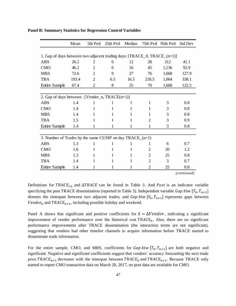
47
Panel B: Summary Statistics for Regression Control Variables
Definitions for 𝑇𝑅𝐴𝐶𝐸𝑖,𝑛 and ∆𝑇𝑅𝐴𝐶𝐸 can be found in Table 3. And 𝑃𝑜𝑠𝑡 is an indicator variable
specifying the post TRACE dissemination (reported in Table 3). Independent variable 𝐺𝑎𝑝 𝑏𝑡𝑤 [𝑇0, 𝑇𝑛+1]
denotes the timespan between two adjacent trades; and 𝐺𝑎𝑝 𝑏𝑡𝑤 [𝑉𝑛, 𝑇𝑛+1] represents gaps between
𝑉𝑒𝑛𝑑𝑜𝑟𝑛 and 𝑇𝑅𝐴𝐶𝐸𝑛+1, including possible holiday and weekend.
Panel A shows that significant and positive coefficients for 𝑋 = ∆𝑉𝑒𝑛𝑑𝑜𝑟 , indicating a significant
improvement of vendor performance over the historical cost 𝑇𝑅𝐴𝐶𝐸0 . Also, there are no significant
performance improvements after TRACE dissemination (the interaction terms are not significant),
suggesting that vendors had other timelier channels to acquire information before TRACE started to
disseminate trade information.
For the entire sample, CMO, and MBS, coefficients for 𝐺𝑎𝑝 𝑏𝑡𝑤 [𝑇0, 𝑇𝑛+1] are both negative and
significant. Negative and significant coefficients suggest that vendors’ accuracy forecasting the next trade
price 𝑇𝑅𝐴𝐶𝐸𝑛+1 decreases with the timespan between 𝑇𝑅𝐴𝐶𝐸0 and 𝑇𝑅𝐴𝐶𝐸𝑛+1. Because TRACE only
started to report CMO transaction data on March 20, 2017, no post data are available for CMO.
Mean 5th Petl 25th Petl Median 75th Petl 95th Petl Std Dev
1. Gap of days between two adjacent trading days: [TRACE_0, TRACE_(n+1)]
ABS 26.2 2 6 12 28 312 41.1
CMO 46.2 2 6 16 45 1,136 92.9
MBS 72.6 2 9 27 76 1,668 127.9
TBA 193.4 2 6.5 16.5 218.5 1,064 338.1
Entire Sample 67.4 2 8 25 70 1,668 122.5
2. Gap of days between : [Vendor_n, TRACE(n+1)]
ABS 1.4 1 1 1 1 3 0.8
CMO 1.4 1 1 1 1 3 0.8
MBS 1.4 1 1 1 1 3 0.8
TBA 1.5 1 1 1 2 3 0.9
Entire Sample 1.4 1 1 1 1 3 0.8
3. Number of Trades by the same CUSIP on day TRACE_(n+1)
ABS 1.3 1 1 1 1 6 0.7
CMO 1.6 1 1 1 2 20 1.2
MBS 1.3 1 1 1 2 25 0.8
TBA 1.4 1 1 1 2 3 0.7
Entire Sample 1.4 1 1 1 2 25 0.8
(continued)

48
Panel C: Estimation of Managerial Discretion Reduction from Regression Results (Model 2)
Define managerial discretion as:
𝐷𝑖𝑠𝑐𝑟𝑒𝑡𝑖𝑜𝑛 ≡ 𝑀𝑎𝑛𝑎𝑔𝑒𝑟𝑠′𝑅𝑒𝑝𝑜𝑟𝑡𝑒𝑑 𝑉𝑎𝑙𝑢𝑒 − 𝑅𝑒𝑓𝑒𝑟𝑒𝑛𝑐𝑒 𝑉𝑎𝑙𝑢𝑒
Accordingly, managerial discretion in the pre- and post- vendor periods can be defined as:
𝐸[𝐷𝑖𝑠𝑐𝑟𝑒𝑡𝑖𝑜𝑛𝑝𝑟𝑒] = 𝑇𝑅𝐴𝐶𝐸𝑛+1 − 𝑇𝑅𝐴𝐶𝐸0 = ∆𝑇; 𝐸[𝐷𝑖𝑠𝑐𝑟𝑒𝑡𝑖𝑜𝑛𝑝𝑜𝑠𝑡] = 𝑇𝑅𝐴𝐶𝐸𝑛+1 − 𝑉𝑒𝑛𝑑𝑜𝑟𝑛
where 𝑅𝑒𝑓𝑒𝑟𝑒𝑛𝑐𝑒 𝑉𝑎𝑙𝑢𝑒 = {𝑇𝑅𝐴𝐶𝐸0 𝑓𝑜𝑟 𝑝𝑟𝑒𝑉𝑒𝑛𝑑𝑜𝑟𝑛 𝑓𝑜𝑟 𝑝𝑜𝑠𝑡
. Then the decrease in managerial discretion is:
∆𝐷 = 𝐷𝑖𝑠𝑐𝑟𝑒𝑡𝑖𝑜𝑛𝑝𝑟𝑒 − 𝐷𝑖𝑠𝑐𝑟𝑒𝑡𝑖𝑜𝑛𝑝𝑜𝑠𝑡 = 𝑉𝑒𝑛𝑑𝑜𝑟𝑛 − 𝑇𝑅𝐴𝐶𝐸0 = 𝑉𝑒𝑛𝑑𝑜𝑟𝑛 − 𝑉𝑒𝑛𝑑𝑜𝑟0 ≡ ∆𝑉
∆𝐷 = 𝐷𝑖𝑠𝑐𝑟𝑒𝑡𝑖𝑜𝑛𝑝𝑟𝑒 − 𝐷𝑖𝑠𝑐𝑟𝑒𝑡𝑖𝑜𝑛𝑝𝑜𝑠𝑡 ≡ ∆𝑉 can be precisely estimated from Model 234
:
∆𝑇𝑅𝐴𝐶𝐸 = 𝛼0 + 𝛼1 ∙ ∆𝑉𝑒𝑛𝑑𝑜𝑟 + 𝛼2 ∙ 𝑇𝑟𝑎𝑑𝑒𝐶𝑜𝑢𝑛𝑡 + 𝛼3 ∙ 𝐺𝑎𝑝1 + 𝛼4 ∙ 𝐺𝑎𝑝2 + 𝜖 ⇒ ∆𝑇 ≈ 0.224 + 0.721 × ∆𝑉 − 0.061 × 𝑇𝑟𝑎𝑑𝑒𝐶𝑜𝑢𝑛𝑡 − 0.001 × 𝐺𝑎𝑝1 + 0.001 × 𝐺𝑎𝑝2 ⇒
∆𝑇
∆𝑉≈ 0.721 +
0.224 − 0.061 × 𝑇𝑟𝑎𝑑𝑒𝐶𝑜𝑢𝑛𝑡 − 0.001 × 𝐺𝑎𝑝1 + 0.001 × 𝐺𝑎𝑝2
∆𝑉
For convenience and simplicity, I evaluate the right-hand side using the sample means for each variable,
we have:
∆𝑇
∆𝑉≈ 0.721 +
0.224 − 0.061 × 1 − 0.001 × 25 + 0.001 × 1
0.3077= 1.173
Then, managerial discretion has decreased by:
∆𝐷
𝐷𝑖𝑠𝑐𝑟𝑒𝑡𝑖𝑜𝑛𝑝𝑟𝑒≈
∆𝑉
∆𝑇=
1
1.173= 85.27%
34 It is obvious that 𝑇𝑅𝐴𝐶𝐸0 = 𝑉𝑒𝑛𝑑𝑜𝑟0
Model 2
Coefficients
Means for
Entire Sample
Model 2 Independent Variables
x = ∆Vendor 0.721 0.3077
Trade Count -0.061 1
Gap btw [T0, T(n+1)] -0.001 25
Gap btw [Vn, T(n+1)] 0.001 1
Constant 0.224

49
T A B L E 5
Channel Three - Spoofing the Vendors
(Cancelled-Single Trades)
Panel A1: Schematic Illustration of “Canceled-Single” Trades
Panel A2: Selection Procedure of “Canceled-Single” Trades
Days
1 5 10 15 20
Price
51.5
51
52
52.5
53
53.5
54
54.5
Initial Trade Later Cancellation Slow Reversion
20 daysQuarter End
"Cancelled-Single" Trades Selection ProcedureNo. of
Transactions
% of Dataset1
# Transactions
% of Dataset1
Total Volume
% of Dataset1
Day Volume
Original TRACE (Dataset0) 25,185,925
After Initial Cleaning (Dataset1) 16,020,744 100%
Total Cancelled Tranactions 379,321 2.37%
ABS 6,688 0.04%
CMO 84,279 0.53%
MBS 151,519 0.95%
TBA 136,835 0.85%
Total "Cancelled-Single" Trades 4,144 0.03% 0.02% 0.28%
Total # of Unique CUSIPs for "Cancelled-Single" Trades 4,144 0.03% 0.02% 0.28%
ABS 50 0.00% 0.04% 1.29%
CMO 535 0.00% 0.13% 0.50%
MBS 3,399 0.02% 0.09% 0.20%
TBA 160 0.00% 0.00% 0.01%
(continued)

50
Panel A3: Descriptive Statistics of “Canceled-Single” Trades
Panel A1 illustrates Cancelled-Single trades.
“Cancelled” means that on 𝐷𝑎𝑦0 a trade is posted on TRACE; on 𝐷𝑎𝑦𝐶𝑎𝑛𝑐𝑒𝑙, this exact trade is
cancelled. The average timespan between [𝐷𝑎𝑦0, 𝐷𝑎𝑦𝐶𝑎𝑛𝑐𝑒𝑙] is 4.49 days (Panel A3);
The initial legal agreement of the trade itself is cancelled. The ownership of the security has not
changed hands. No real transaction has ever happened;
“Single” means the cancelled transaction is the only trade for the particular CUSIP on 𝐷𝑎𝑦0, that
is, there are no parallel, concurrent, or side trades for the same CUSIP on 𝐷𝑎𝑦0;
There are no other trades between [𝐷𝑎𝑦0, 𝐷𝑎𝑦𝐶𝑎𝑛𝑐𝑒𝑙] for this particular security, there are no
contamination nor interference from the inter [𝐷𝑎𝑦0, 𝐷𝑎𝑦𝐶𝑎𝑛𝑐𝑒𝑙] trades;
Cancelled-Single trades provide a very clear setting to test vendors’ asymmetric response to the
advent and disappearance of the same economic information.
Panel A2 indicates that the scope of the Cancelled-Single trades is very limited. Out of the 16,020,744
total transactions, there are only 4,144 Cancelled-Single trades, with 50 from ABS, 535 from CMO, 3,399
from MBS, and 160 from TBA. These Cancelled-Single trades are quite rare, and account for only 0.02%
of the total trading volume of the entire sample and 0.28% of the daily trading volume.
Panel A3 shows that on average, cancellations occur 4.49 days after the initial posted transactions,
slightly longer than those from the entire sample (3.90).
Mean STD Max75%
Q3Median Mean STD
75%
Q3Median
Security Type
ABS 50 4.58 4.37 20 6 3 2.94 2.91 2 4
CMO 535 3.62 3.79 27 5 2 3.85 3.90 3 5
MBS 3,399 4.48 6.33 27 4 2 3.44 3.69 2 4
TBA 160 7.54 8.14 28 10 4 4.56 4.95 3 6
Entire Sample 4,144 4.49 6.16 28 5 2 3.90 4.18 5 2
(continued)
Days between Initial Report and Later Cancellation
"Canceled-Single Trades" Entire Sample
Days between Report and CancellationNo. of
Security
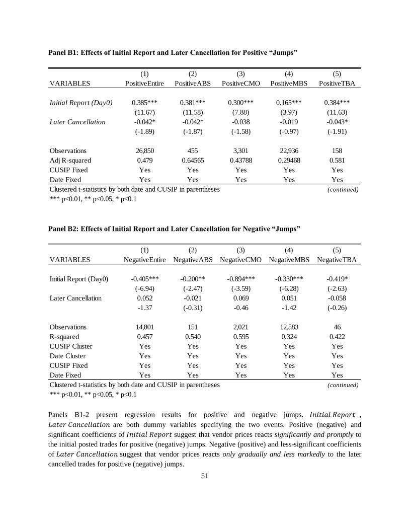
51
Panel B1: Effects of Initial Report and Later Cancellation for Positive “Jumps”
Panel B2: Effects of Initial Report and Later Cancellation for Negative “Jumps”
Panels B1-2 present regression results for positive and negative jumps. 𝐼𝑛𝑖𝑡𝑖𝑎𝑙 𝑅𝑒𝑝𝑜𝑟𝑡 ,
𝐿𝑎𝑡𝑒𝑟 𝐶𝑎𝑛𝑐𝑒𝑙𝑙𝑎𝑡𝑖𝑜𝑛 are both dummy variables specifying the two events. Positive (negative) and
significant coefficients of 𝐼𝑛𝑖𝑡𝑖𝑎𝑙 𝑅𝑒𝑝𝑜𝑟𝑡 suggest that vendor prices reacts significantly and promptly to
the initial posted trades for positive (negative) jumps. Negative (positive) and less-significant coefficients
of 𝐿𝑎𝑡𝑒𝑟 𝐶𝑎𝑛𝑐𝑒𝑙𝑙𝑎𝑡𝑖𝑜𝑛 suggest that vendor prices reacts only gradually and less markedly to the later
cancelled trades for positive (negative) jumps.
(1) (2) (3) (4) (5)
VARIABLES PositiveEntire PositiveABS PositiveCMO PositiveMBS PositiveTBA
Initial Report (Day0) 0.385*** 0.381*** 0.300*** 0.165*** 0.384***
(11.67) (11.58) (7.88) (3.97) (11.63)
Later Cancellation -0.042* -0.042* -0.038 -0.019 -0.043*
(-1.89) (-1.87) (-1.58) (-0.97) (-1.91)
Observations 26,850 455 3,301 22,936 158
Adj R-squared 0.479 0.64565 0.43788 0.29468 0.581
CUSIP Fixed Yes Yes Yes Yes Yes
Date Fixed Yes Yes Yes Yes Yes
Clustered t-statistics by both date and CUSIP in parentheses (continued)
*** p<0.01, ** p<0.05, * p<0.1
(1) (2) (3) (4) (5)
VARIABLES NegativeEntire NegativeABS NegativeCMO NegativeMBS NegativeTBA
Initial Report (Day0) -0.405*** -0.200** -0.894*** -0.330*** -0.419*
(-6.94) (-2.47) (-3.59) (-6.28) (-2.63)
Later Cancellation 0.052 -0.021 0.069 0.051 -0.058
-1.37 (-0.31) -0.46 -1.42 (-0.26)
Observations 14,801 151 2,021 12,583 46
R-squared 0.457 0.540 0.595 0.324 0.422
CUSIP Cluster Yes Yes Yes Yes Yes
Date Cluster Yes Yes Yes Yes Yes
CUSIP Fixed Yes Yes Yes Yes Yes
Date Fixed Yes Yes Yes Yes Yes
Clustered t-statistics by both date and CUSIP in parentheses (continued)
*** p<0.01, ** p<0.05, * p<0.1
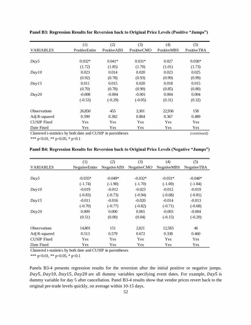
52
Panel B3: Regression Results for Reversion back to Original Price Levels (Positive “Jumps”)
Panel B4: Regression Results for Reversion back to Original Price Levels (Negative “Jumps”)
Panels B3-4 presents regression results for the reversion after the initial positive or negative jumps.
𝐷𝑎𝑦5, 𝐷𝑎𝑦10, 𝐷𝑎𝑦15, 𝐷𝑎𝑦20 are all dummy variables specifying event dates. For example, 𝐷𝑎𝑦5 is
dummy variable for day 5 after cancellation. Panel B3-4 results show that vendor prices revert back to the
original pre-trade levels quickly, on average within 10-15 days.
(1) (2) (3) (4) (5)
VARIABLES PositiveEntire PositiveABS PositiveCMO PositiveMBS PositiveTBA
Day5 0.032* 0.041* 0.031* 0.027 0.036*
(1.72) (1.85) (1.70) (1.01) (1.73)
Day10 0.023 0.014 0.020 0.023 0.025
(0.92) (0.78) (0.93) (0.99) (0.99)
Day15 0.011 0.015 0.020 0.018 0.015
(0.70) (0.78) (0.90) (0.85) (0.80)
Day20 -0.008 -0.004 -0.001 0.004 0.004
(-0.53) (-0.29) (-0.05) (0.31) (0.32)
Observations 26,850 455 3,301 22,936 158
Adj R-squared 0.599 0.382 0.804 0.367 0.489
CUSIP Fixed Yes Yes Yes Yes Yes
Date Fixed Yes Yes Yes Yes Yes
Clustered t-statistics by both date and CUSIP in parentheses (continued)
*** p<0.01, ** p<0.05, * p<0.1
(1) (2) (3) (4) (5)
VARIABLES NegativeEntire NegativeABS NegativeCMO NegativeMBS NegativeTBA
Day5 -0.035* -0.049* -0.032* -0.031* -0.040*
(-1.74) (-1.90) (-1.70) (-1.69) (-1.84)
Day10 -0.019 -0.012 -0.023 -0.012 -0.019
(-0.83) (-0.73) (-0.94) (-0.68) (-0.81)
Day15 -0.011 -0.016 -0.020 -0.014 -0.013
(-0.70) (-0.77) (-0.82) (-0.71) (-0.68)
Day20 0.009 0.000 0.001 -0.003 -0.004
(0.51) (0.00) (0.04) (-0.15) (-0.20)
Observations 14,801 151 2,021 12,583 46
Adj R-squared 0.513 0.579 0.672 0.338 0.460
CUSIP Fixed Yes Yes Yes Yes Yes
Date Fixed Yes Yes Yes Yes Yes
Clustered t-statistics by both date and CUSIP in parentheses
*** p<0.01, ** p<0.05, * p<0.1

53
T A B L E 6
Channel Three - Spoofing the Vendors
(Comparison of “Canceled-Single” Trades to Normal Trades)
Panel A: % of Dealer-Customer Trade (Cancelled-Single Trades vs. Entire Sample)
Cancelled Single Trade Entire Sample
Security Type
ABS 90.70% 75.16% ***
CMO 80.84% 60.13% ***
MBS 92.15% 52.03% ***
TBA 88.78% 23.49% ***
Total 89.00% 36.68% *** *** p<0.01, ** p<0.05, * p<0.1
% of Dealer_Customer Trade
Percentage
Difference
Significance
Panel B: Descriptive Statistics for Trading Volume of Cancelled-Single Trades vs. Non-cancelled Normal Trades (Controls)
Security TypeOrder
Status
No. of
Trades
Mean Volume
($10,000)5th Petl 25th Petl Median 75th Petl 95th Petl Std Dev
Cancelled-Single 43 1,685 0.4 65 178 953 3,141 5,813
Normal Control 1,500 611 3.25 35 131 500 2,627 1,491
Cancelled-Single 426 4,891 0.3 10 256 1,520 10,000 57,438
Normal Control 8,626 517 0.5 3 13 200 2,728 2,379
Cancelled-Single 2,902 716 2.996 48 145 444 2,914 2,474
Normal Control 30,389 638 1 9 82 272 2,299 11,569
Cancelled-Single 122 1,501 38.27 207 860 1,908 5,000 1,838
Normal Control 1,519 1,104 47.2986 191 500 1,130 4,520 1,905
Cancelled-Single 3,493 1,264 2.5 47 156 536 4,006 20,224
Normal Control 42,034 629 0.8 7 75 300 2,500 9,907
ABS
CMO
MBS
TBA
Entire Sample

54
Panel C: Cancelled-Single Trades vs. Normal Trades for the Same CUSIP at Different Times
𝑇𝑟𝑎𝑑𝑖𝑛𝑔𝑉𝑜𝑙𝑢𝑚𝑒𝑖𝑡 = 𝛼0 + 𝛼1 ∙ 𝐶𝑎𝑛𝑐𝑒𝑙𝑒𝑑𝑆𝑖𝑛𝑔𝑙𝑒𝐼𝑛𝑑𝑖𝑐𝑎𝑡𝑜𝑟𝑖𝑡 + 𝐶𝑜𝑛𝑡𝑟𝑜𝑙𝑠 + 𝜖𝑖𝑡
This table presents comparison of “Canceled-Single” trades to normal non-cancelled trades (controls).
Panel A shows that the percentage of dealer-customer trades are significantly higher in Cancelled-Single
trades than the entire sample. According to FINRA rules, in trades between a dealer and a customer, only
the dealer need to report to TRACE, while in an inter-dealer trade, both dealers need to report to TRACE.
Therefore, price manipulation in inter-dealer trades requires a higher level of collusion than the dealer-
customer trades.
Panel B shows the comparison of trading volumes of “Canceled-Single” trades vs. normal non-cancelled
trades (controls) for the same security. The trading volumes for “Canceled-Single” trades are generally
(significantly) larger than those of the controls.
Panel C shows the regression results. 𝑇𝑟𝑎𝑑𝑖𝑛𝑔𝑉𝑜𝑙𝑢𝑚𝑒 is the dollar value of a trade in ($10,000),
𝐶𝑎𝑛𝑐𝑒𝑙𝑒𝑑𝑆𝑖𝑛𝑔𝑙𝑒𝐼𝑛𝑑𝑖𝑐𝑎𝑡𝑜𝑟 is an indicator variable where 𝐶𝑎𝑛𝑐𝑒𝑙𝑒𝑑𝑆𝑖𝑛𝑔𝑙𝑒𝐼𝑛𝑑𝑖𝑐𝑎𝑡𝑜𝑟 = 1 for Canceled-
Single trades and 0 for normal non-cancelled trades. Control variables include liquidity score, Weighted
Average Life (WAL), trade counts, and gap between trades. Data is winsorized at 5% and 95%. For the
same security, trading volumes for Canceled-Single trades are significantly higher than those for normal
non-cancelled trades.
Results from Panels B and C suggest that in order to augment the spoofing effects, bank managers have to
post an artificially and significantly higher volume to make the spoofing trades more “sensational”.
(1) (2) (3) (4) (5)
VARIABLES Entire ABS CMO MBS TBA
Canceled vs. Normal 122.643*** 69.227*** 198.061*** 113.253*** 46.578***
(9.80) (3.55) (4.80) (8.43) (3.38)
Observations 37,208 1,049 5,767 28,570 1,125
Adj R-squared 0.06778 0.51651 0.31619 0.08679 0.51632
CUSIP Fixed Yes Yes Yes Yes Yes
Date Fixed No No No No No
Controls Yes Yes Yes Yes Yes
Clustered t-statistics by both date and CUSIP in parentheses
*** p<0.01, ** p<0.05, * p<0.1

55
References
Ahmed, A.S., C. Takeda, and S. Thomas. 1999. Bank loan loss provisions: A re-examination of capital
management, earnings management and signalling effects. Journal of Accounting and Economics 28 (1):
1-25.
Barth, M. E. 1994. Fair value accounting: Evidence from investment securities and the market valuation
of banks. The Accounting Review 69 (1): 1-25.
Barth, M. E., W. R. Landsman, and J. M. Wahlen. 1995. Fair value accounting: Effects on banks' earnings
volatility, regulatory capital, and value of contractual cash flows. Journal of Banking and Finance 19 (3-
4): 577-605.
Barth, M. E., W. H. Beaver, and W. R. Landsman. 1996. Value-relevance of banks’ fair value disclosures
under SFAS No. 107. The Accounting Review 71 (4): 513-537.
Barth, M., M. McNichols, P. Wilson. 1997. Factors Influencing Firms’ Disclosures about Environmental
Liabilities. Review of Accounting Studies 2 (1): 35-64.
Barth, M. E., J. Gomez-Biscarri, R. Kasznik and G. Lopez-Espinosa. 2012. Fair value accounting,
earnings management and the use of available-for-sale instruments by bank managers. Working paper,
Stanford University.
Barth, M. E., J. Gomez-Biscarri, R. Kasznik and G. Lopez-Espinosa. 2014. Bank Earnings and
Regulatory Capital Management using Available for Sale Securities. Working paper, Stanford University.
Beatty, A., B. L. Chamberlain, and J. Magliolo. 1995. Managing financial reports of commercial banks:
The influence of taxes, regulatory capital, and earnings. Journal of Accounting Research 33 (2): 231-261.
Beatty, A., and D. G. Harris. 1999. The effects of taxes, agency costs and information asymmetry on
earnings management: A comparison of public and private firms. Review of Accounting Studies 3 (3-4):
299-326.
Beatty, A., and S. Liao. 2014. Financial accounting in the banking industry: a review of the empirical
literature. Journal of Accounting and Economics 58 (2014): 339-383.
Beatty, A. L., B. Ke, and K. R. Petroni. 2002. Earnings management to avoid earnings declines across
publicly and privately held banks. The Accounting Review 77 (3): 547-570.
Beaver, W. H., and E. E. Engel. 1996. Discretionary behavior with respect to allowances for loan losses
and the behavior of security prices. Journal of Accounting and Economics 22 (1-3): 177-206.
Benson, B. and M. Teclezion. 2007. The status of fair value accounting. iNews winter, issue 1. iComp
L.L.C..
Benston, G. J. 2008. The shortcomings of fair-value accounting described in SFAS 157. Journal of
Accounting and Public Policy 27 (2): 101-114.

56
Blankespoor, E., T. J. Linsmeier, K. Petroni and C. Shakespeare. 2013. Fair value accounting for financial
instruments: Does it improve the association between bank leverage and credit risk? The Accounting
Review Vol. 88, No.4 1143-1177
Board of Governors of the Federal Reserve System. 2007. Instructions for preparation of consolidated
financial statements for bank holding companies. Chicago, IL.
Bratten, B., M. Causholli and U. Khan. 2011. Fair value accounting and the predictive ability of earnings
Evidence from the Banking Industry. Working Paper, University of Kentucky.
Bratten, B., M. Causholli and L. Myers. 2013. The effect of fair value accounting and auditor
specialization on earnings management: evidence from the banking industry. Working Paper, University
of Kentucky.
Burgstahler, D., and I. Dichev. 1997. Earnings management to avoid earnings decreases and losses.
Journal of Accounting and Economics 24 (December): 99-126.
Chen, F., K. Lam, W. Smieliauskas, and M. Ye. 2014. Auditor Conservatism and Banks’ Measurement
Uncertainty during the Financial Crisis. Working Paper, University of Toronto.
Collins, J., D. Shackelford, and J. Wahlen. 1995. Bank differences in the coordination of regulatory
capital, earnings, and taxes. Journal of Accounting Research 33 (2): 263-291.
Dechow, P., L. Myers, and C. Shakespeare. 2010. Fair Value Accounting and Gains from Asset
Securitizations: A Convenient Earnings Management Tool with Compensation Side-Benefits. Journal of
Accounting and Economics 49 (1): 2-25.
DeFond, M. 2010. Earnings Quality Research: Advances, Challenges and Future Research. Journal of
Accounting and Economics 50 (2010) 402-409.
Degeorge, F., J. Patel, and R. Zeckhauser. 1999. Earnings Management to Exceed Thresholds. Journal of
Business 72 (1): 1-33.
Dichev, Ilia D., John Graham, Campbell Harvey, and Shiva Rajgopal, 2013, Earnings quality: Evidence
from the field, Journal of Accounting and Economics 56 (2013) 1–33.
Dick-Nielsen Jens 2014, How to Clean Enhanced TRADE Data. Working Paper.
Ettredge, M., Y. Xu, and H. Yi. 2010. Fair value measurements, auditor industry expertise and audit fees:
Evidence from the banking industry. Working Paper, University of Kansas.
Fiechter, P., and C. Meyer. 2010. Big bath accounting using fair value measurement discretion during the
financial crisis. Working Paper, University of Zurich.
Financial Accounting Standards Board (FASB). 2006. Fair Value Measurements. Statement of Financial
Accounting Standards No. 157. Norwalk, CT.
Financial Accounting Standards Board (FASB). 2007. The Fair Value Option for Financial Assets and
Financial Liabilities. Statement of Financial Accounting Standards No. 159. Norwalk, CT.
57
Graham, J., C. Harvey, and S. Rajpopal. 2005. The economic implications of corporate financial
reporting. Journal of Accounting and Economics 40: 3-37.
Gow, I., Larcker, D., Reiss, P. 2016. Causal Inference in Accounting Research. Journal of Accounting
Research 54: 477-523.
Heflin, F. and A. Valencia. 2012. Opportunistic behavior using level 3 fair values under SFAS 157.
Working paper, Florida State University.
Kanagaretnam, K., G. J. Lobo, and R. Mathieu. 2003. Managerial incentives for income smoothing
through bank loan loss provisions. Review of Quantitative Finance and Accounting 20 (1): 63-80.
Kanagaretnam, K., G. V. Krishnan, and G. J. Lobo. 2009. Is the market valuation of banks’ loan loss
provision conditional on auditor reputation? Journal of Banking and Finance 33 (6): 1039-1047.
Kim, M. and W. Kross. 1998. The impact of the change in bank capital standards on loan loss provisions
and loan write-offs. Journal of Accounting and Economics 25 (1): 69-99.
Liang, Lihong and Riedl, Edward J. (2014) The Effect of Fair Value versus Historical Cost Reporting
Model on Analyst Forecast Accuracy. The Accounting Review: May 2014, Vol. 89, No. 3, pp. 1151-1177.
Liao, L., H. Kang, R. Morris, and Q. Tang. 2010. Information asymmetry of fair value accounting and
loan loss provisions during the global financial crisis. Working Paper, University of New South Wales.
Liu, J., E., Riedl. 2017. The Effect of Independent Third-party Vendors’ Evaluated Prices on Bank
Managers’ Discretion over Fair Values. Working paper.
Liu, J. 2017. The Effect of Independent Third-party Vendors’ Evaluated Prices on Real Transaction
Based Earning and Capital Management. Working paper, Harvard Business School.
Lobo, G. J and D. Yang. 2001. Bank managers’ heterogeneous decisions on discretionary loan loss
provisions. Review of Quantitative Finance and Accounting 16 (3): 223-250.
Martin, R. D., J. S. Rich., and T. J. Wilks. 2006. Auditing fair value measurements: A synthesis of
relevant research. Accounting Horizons 20 (3): 287-303.
Matthews, W. J. 2011. Stimulus Repetition and the Perception of Time: The Effects of Prior Exposure on
Temporal Discrimination, Judgment, and Production. PLoS ONE, 6(5), e19815.
http://doi.org/10.1371/journal.pone.0019815
Moyer, S. 1990. Capital adequacy ratio regulations and accounting choices in commercial banks. Journal
of Accounting and Economics 13 (2): 123-154.
Nelson, K. K. 1996. Fair value accounting for commercial banks: An empirical analysis of SFAS No.
107. The Accounting Review 71 (2): 161-182.
Nichols, D.C., J. M. Wahlen and M. M. Wieland. 2009. Publicly traded versus privately held:
Implications for conditional conservatism in bank accounting. Review of Accounting Studies 14 (1): 88-
122.

58
Riedl, E. J., and G. Serafeim. 2011. Information Risk and Fair Values: An Examination of Equity Betas.
Journal of Accounting Research 49 (4): 1083-1122.
Ryan, S. G. 2007. Financial instruments and institutions: Accounting and disclosure rules, 2nd
edition.
John Wiley & Sons, Inc., New Jersey.
Ryan, S. G. 2008. Accounting in and for the subprime crisis. The Accounting Review 83 (6): 1605-1638..
Scholes, M.S., G.P. Wilson, and M.A. Wolfson. 1990. Tax planning, regulatory capital planning, and
financial reporting strategy for commercial banks. The Review of Financial Studies 3 (4): 625-650.
Song, C. J. 2008. An evaluation of FAS 159 fair value option: Evidence from the banking industry.
Working Paper, Virginia Polytechnic Institute and State University.
Song, C. J., W. Thomas, and H. Yi. 2010. Value relevance of FAS 157 fair value hierarchy information
and the impact of corporate governance mechanisms. The Accounting Review 85 (4): 1375-1410.
Wahlen, J. M. 1994. The nature of information in commercial bank loan loss disclosures. The Accounting
Review 69 (3): 455-478.
Warfield, T.D, J. J. Wild, and K. L. Wild. 1995. Managerial ownership, accounting choices, and
informativeness of earnings. Journal of Accounting and Economics 20 (1): 61-91.
Lepper, M. R., Greene, D., and R. E. Nisbett. 1973. Undermining children's intrinsic interest with
extrinsic reward: A test of the ‘overjustification’ hypothesis. Journal of Personality and Social
Psychology, 28(1): 129-137.
Locke, E. A., and G. P. Latham. 1990. A Theory of Goal Setting and Task Performance. Englewood
Cliffs, NJ: Prentice Hall.
Locke, E. A., and G. Latham. 2002. Building a practically useful theory of goal setting and task
motivation. American Psychologist 57 (9): 705–717.
Maignan, I. and Ralston, D. A. 2002. Corporate Social Responsibility in Europe and the US: Insights
from Businesses' Self-Presentations. Journal of International Business Studies, 33(3): 497-515.
Margolis, J. D. and Walsh, J. P. 2003. Misery loves companies: Rethinking social initiatives by business.
Administrative Science Quarterly, 48(2): 268-305.
Margolis, Joshua D. and Elfenbein, Hillary Anger and Walsh, James P.. 2009. Does it Pay to Be
Good...And Does it Matter? A Meta-Analysis of the Relationship between Corporate Social and Financial
Performance. Working paper.
Markman, A. B., W. T. Maddox, and D. A. Worthy. 2006. Choking and excelling under pressure.
Psychological Science, 17 (11): 944–948.
Mas A, Moretti E. 2009. Peers at work. American Economic Review, 99 (1): 112–145.
Matsumura, E., R. Prakash, and S. Vera-Munoz. 2014. Firm-value effects of carbon emissions and carbon
disclosures. The Accounting Review, 89 (2): 695-724.

59
Merchant, K. A., and J. F. Manzoni. 1989. The achievability of budget targets in profit centers: A field
study. The Accounting Review, 64 (3): 539–558.
Neu, D., H. Warsame, and K. Pedwell. 1997. Managing Public Impressions: Environmental Disclosures
in Annual Reports. Accounting, Organizations and Society 23 (3): 265-282.
Oyer P. 1998. Fiscal year ends and non-linear incentive contracts: the effect on business seasonality.
Quarterly Journal of Economics 113: 149–185.
Paarsch H, Shearer B. 2000. Piece rates, fixed wages, and incentive effects: statistical evidence from
payroll records. International Economic Review 41: 59–92.
Porter M. and C. van der Linde. 1995. Toward a New Conception of the Environment-Competitiveness
Relationship. The Journal of Economic Perspectives 9 (4): 97-118.
Prendergast, C. 1999. The Provision of Incentives in Firms. Journal of Economic Literature, 37 (1): 7-63
Shalley, C. E. 1991. Effects of productivity goals, creativity goals, and personal discretion on individual
creativity. Journal of Applied Psychology 76 (1): 179–185.
Shalley, C. E. 1995. Effects of coaction, expected evaluation, and goal setting on creativity and
productivity. Academy of Management Journal 38 (2): 483–503.
Skinner, B. F. 1953. Science and human behavior. New York: Macmillan.
Thompson, K. R., W. Hochwarter, and N. Mathys. 1997. Stretch targets: What makes them effective? The
Academy of Management Executive 11 (3): 48–60.
Williamson, M.G., and Zhang, Y. M. 2013. Productivity-Target Difficulty, Target-Based Pay, and
Outside-the-Box Thinking." The Accounting Review 88 (4): 1433-1457.