Embed Size (px)
Citation preview

Delft University of Technology
Accuracy Enhancement and Filtering forVisualisation of Discontinuous Solutions
Prof. Kees Vuik
Dr. Jennifer K. Ryan
Paulien van Slingerland
Delft University of Technology
TU Berlin, 15 December 2009
15 December 2009 – p.1/43
Delft University of Technology
Accuracy Enhancement and Filtering for Visualisation of Discontinuous Solutions
Motivation and Background Discontinuous Galerkin Method Post-Processing for Accuracy Enhancement Applications in Visualisation
Issues and challenges non-uniform mesh derivative post-processing ⇒ one-sided post-processing ⇐
Summary
15 December 2009 – p.2/43

Delft University of Technology
1D Discontinuous Galerkin Formulation
Define a Mesh and an Approximation Space:
Ij = (xj −xj
2, xj +
xj
2), j = 1, · · · , N and Vh = φ
(l)j (x) ∈ P
k|Ij, j = 1, · · · , N
Consider ut + f(u)x = 0.
Weak Formulation: Find uh(x, t) ∈ Vh such that
Z
Ij
(uh)tvdx =
Z
Ij
f(uh)vxdx− f((uh)j+ 12
)vj+ 12
+ f((uh)j− 12
)vj− 12
for all v ∈ Vh.
15 December 2009 – p.3/43

Delft University of Technology
1D Discontinuous Galerkin Formulation
Numerical Scheme:
Z
Ij
(uh)tvdx =
Z
Ij
f(uh)vxdx− fj+1/2v−
j+1/2+ fj−1/2v
+j−1/2
∀v ∈ Vh.
• Use upwind monotone flux
• Take v from inside the cell
DG solution: uh(x, t) =∑k
l=0 u(l)i (t)φ
(l)i (x) if x ∈ Ii.
15 December 2009 – p.4/43

Delft University of Technology
Can we improve an existing DG approximation?
15 December 2009 – p.5/43

Delft University of Technology
Post-Processing to Improve and Approximation
The post-processor:
u⋆ = K2(k+1),k+1h ⋆ uh
Why do we post-process? Errors in DG solution are highly oscillatory Post-processing filters out oscillations around the exact
solution Result is a solution that has increased smoothness and
accuracy
15 December 2009 – p.6/43

Delft University of Technology
Post-Processor
B. Cockburn, M. Luskin, C.-W. Shu, A. S uli, Math Comp. (2003)
Discontinuous Galerkin approximation errors:
||uh − u||−l = O(h2k+1),
whereas in the L2−norm we have
||uh − u||2 = O(hk+1).
Post-processor extracts this information.
u∗(x) = Kh ∗ uh
• Works for a locally uniform mesh:−→ Translation invariant
−→ Post-Processor is local15 December 2009 – p.7/43

Delft University of Technology
Negative Order Sobolev Norm
The negative order norm is given by
||u||−ℓ,Ω = supφ∈C∞
0
∫
Ωu(x)φ(x)dx
||φ||ℓ,Ω, ℓ ≥ 1,
which is just a seminorm divided by the usual Sobolev norm.
Example: For the function uN = sin(2πNx), Ω = (−1, 1), ℓ ≥ 1, thenegative order norm is
||uN ||−ℓ,Ω =1
(2πN)ℓ
The negative order norm tells us that sin(2πNx) oscillates around zerofairly regularly.
15 December 2009 – p.8/43

Delft University of Technology
Bramble & Schatz, Math. Comp. (1977)
Mock & Lax, Comm. Pure Appl. Math (1978)
Post-Processor Kernel
Independent of the partialdifferential equation.
Applied only at the final time. Filters out oscillations in the
error.
Kernel Properties
Compact Support ⇒Computationally advantages
Reproduces polynomials ofdegree 2k by convolution. ⇒Accuracy is not lost.
Linear combination ofB-splines.
15 December 2009 – p.9/43

Delft University of Technology
Post-Processor
Use Negative order norms ⇒ Tells us how oscillatory a function is(difficult to compute).
Use Convolution ⇒ “Filters” out these oscillations B-splines ⇒ Gives the convolution kernel nice properties. Make assumptions on the approximation and the mesh.
Result: A post-processor that filters out oscillations in the error andimproves the order of accuracy.
15 December 2009 – p.10/43

Delft University of Technology
Kernel Construction
Post-processed solution: u⋆(x) = K2(k+1),k+1h ⋆ uh.
K2(k+1),k+1h (x) =
1
h
k∑
γ=−k
c2(k+1),k+1γ ψ(k+1)
(x
h− γ
)
h = xi for all i, and c2(k+1),k+1γ ∈ R.
B-spline recursion formula:
ψ(1) = χ[−1/2,1/2],
ψ(k+1) =1
k
»„
x+k + 1
2
«
ψ(k)
„
x+1
2
«
+
„
k + 1
2− x
«
ψ(k)
„
x−1
2
«–
, k ≥ 1.
15 December 2009 – p.11/43
Delft University of Technology
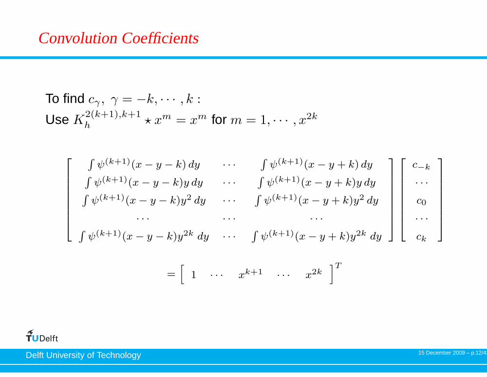
Convolution Coefficients
To find cγ , γ = −k, · · · , k :
Use K2(k+1),k+1h ⋆ xm = xm for m = 1, · · · , x2k
2
6
6
6
6
6
6
6
4
R
ψ(k+1)(x− y − k) dy · · ·R
ψ(k+1)(x− y + k) dyR
ψ(k+1)(x− y − k)y dy · · ·R
ψ(k+1)(x− y + k)y dyR
ψ(k+1)(x− y − k)y2 dy · · ·R
ψ(k+1)(x− y + k)y2 dy
· · · · · · · · ·R
ψ(k+1)(x− y − k)y2k dy · · ·R
ψ(k+1)(x− y + k)y2k dy
3
7
7
7
7
7
7
7
5
2
6
6
6
6
6
6
6
4
c−k
· · ·
c0
· · ·
ck
3
7
7
7
7
7
7
7
5
=h
1 · · · xk+1 · · · x2kiT
15 December 2009 – p.12/43
Delft University of Technology
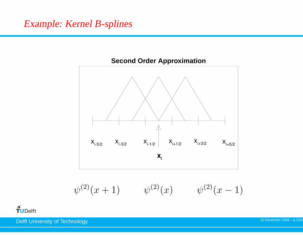
Example: Kernel B-splines
Second Order Approximation
ψ(2)(x+ 1) ψ(2)(x) ψ(2)(x− 1)
15 December 2009 – p.13/43

Delft University of Technology
Kernel for Linear Approximation
Find cγ , γ = −1, 0, 1 : Use K4,2h ⋆ p = p for p = 1, x, x2
−2.5 −2 −1.5 −1 −0.5 0 0.5 1 1.5 2 2.5 −0.5
0
0.5
1
1.5
Ij
Ij−1I
j−2Ij+1
Ij+2
K4,2(x) =−1
12ψ(2)(x− 1) +
7
6ψ(2)(x) −
1
12ψ(2)(x+ 1)
15 December 2009 – p.14/43

Delft University of Technology
Implementing the Post-processor
For element Ij = (xj−1/2,j+1/2) :
⇒ u⋆(x) =∑
i
k∑
l=0
uli
k∑
γ=−k
c2(k+1),k+1γ
∫
ψ(k+1)
(x− y
h− γ
)
φ(l)i (y) dy.
where i = j − p′, · · · , j + p′, p′ = ⌈ 3k+12 ⌉
k 1 2 3
p’ 2 3 5
Note: p′ is the number of elements needed on each side of theelement being post-processed.
15 December 2009 – p.15/43

Delft University of Technology
Example: Implementingk = 1 case
−1.5 −1 −0.5 0 0.5 1 1.5−0.4
−0.2
0
0.2
0.4
0.6
0.8
1
Ij
Ij−1 I
j+1
green line = DG
approximation on one
element.
blue line = kernel. The
kernel is introducing
smoothness at the element
boundaries.
Convolution Kernel:
K4,2(x) =−1
12ψ(2)(x− 1) +
7
6ψ(2)(x) −
1
12ψ(2)(x+ 1)
Discontinuous Galerkin Solution: uh(x) = u(0)j φ
(0)j + u
(1)j φ
(1)j
on element Ij = (xj−1/2, xj+1/2).
15 December 2009 – p.16/43

Delft University of Technology
2−D Kernel
The 2−D case is simply a tensor product of the 1−D case.
Kernel:
Kh =1
hxhy
k∑
γx=−k
k∑
γy=−k
cγxcγyψ(k+1)
(x
hx− γx
)
ψ(k+1)
(y
hy− γy
)
We can use either a tensor product of polynomials, Qk - (1, x, y, xy),or the usual polynomial basis, Pk - (1, x, y).
15 December 2009 – p.17/43

Delft University of Technology 15 December 2009 – p.18/43

Delft University of Technology
1 −D Variable Coefficient Equation
Ryan, Shu, Atkins, SISC (2005)
uh(x, 12.5) u∗(x, 12.5)
mesh L2 error order L2 error order
P1
10 1.83E-02 — 7.82E-02 —
20 4.35E-03 2.07 1.08E-03 2.86
40 1.07E-03 2.03 1.39E-04 2.96
P2
10 8.61E-04 — 1.34E-04 —
20 1.07E-04 3.01 2.34E-06 5.84
40 1.34E-05 3.00 4.55E-08 5.69
ut + (au)x = f
a(x) = 2 + sin(x)
u(x, 0) = sin(3x)
u(0, t) = u(2π, t)T = 12.5
15 December 2009 – p.19/43

Delft University of Technology
Applications in Filtering for Visualisation
Streamline Calculation: Filtering Entire Field
Obtain numerical approximation Post-Process the approximation We can then choose our time integrator for the streamline
calculation (such as RK-4)
d
dt~x(t) = ~F (~x(t))
~x(t = 0) = ~x0
The post-processor increases smoothness of the approximationto help obtain the correct streamline.
15 December 2009 – p.20/43

Delft University of Technology
Applications in Filtering for Streamline Visualisation
Example Field: Scheuerman, Tricoche, and Hagen, IEEE Vis (1999).
Steffan, Curtis, Kirby, and Ryan, IEEE-TVCG (2008).
−0.8 −0.6 −0.4 −0.2 0 0.2 0.4 0.6 0.8
−0.8
−0.6
−0.4
−0.2
0
0.2
0.4
0.6
0.8
(u, v)T = ~F (x, y), Ω = [−1, 1] × [−1, 1]
z = x+ ıy
u = Re(r)
v = −Im(r).
r = (z − (0.74 + 0.35ı))(z − (0.68 − 0.59ı))
(z − (−0.11 − 0.72ı))(z − (−0.58 + 0.64
(z − (0.51 − 0.27ı))(z − (−0.12 + 0.84
15 December 2009 – p.21/43
Delft University of Technology
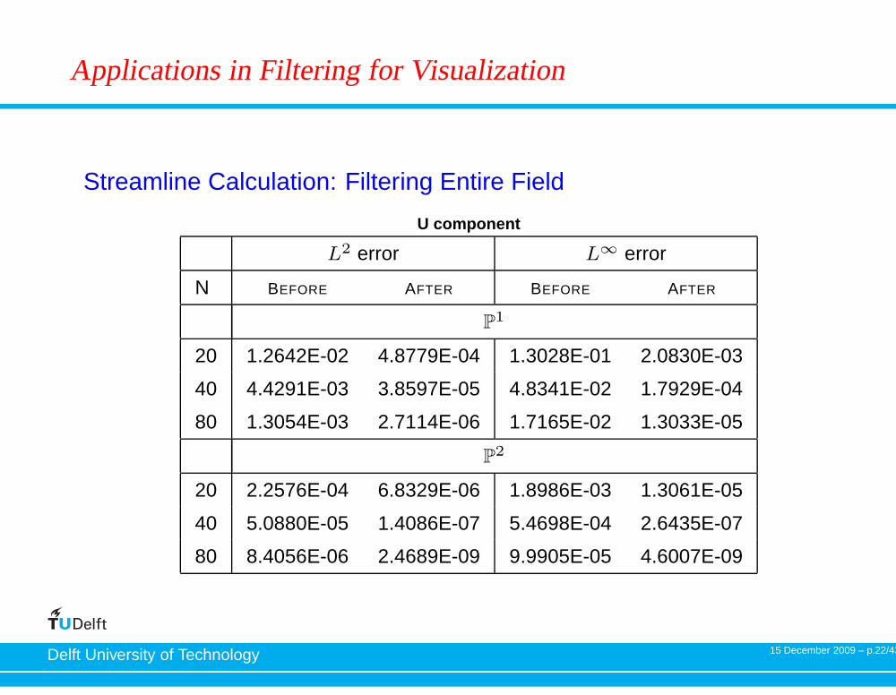
Applications in Filtering for Visualization
Streamline Calculation: Filtering Entire Field
U component
L2 error L∞ error
N BEFORE AFTER BEFORE AFTER
P1
20 1.2642E-02 4.8779E-04 1.3028E-01 2.0830E-03
40 4.4291E-03 3.8597E-05 4.8341E-02 1.7929E-04
80 1.3054E-03 2.7114E-06 1.7165E-02 1.3033E-05
P2
20 2.2576E-04 6.8329E-06 1.8986E-03 1.3061E-05
40 5.0880E-05 1.4086E-07 5.4698E-04 2.6435E-07
80 8.4056E-06 2.4689E-09 9.9905E-05 4.6007E-09
15 December 2009 – p.22/43
Delft University of Technology
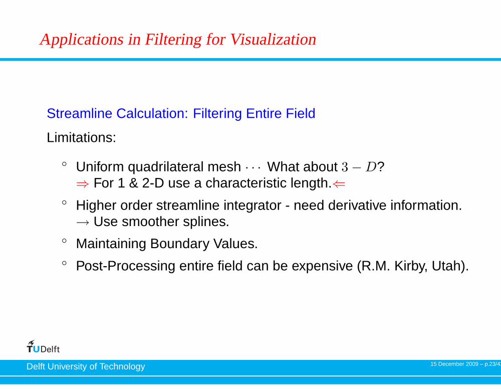
Applications in Filtering for Visualization
Streamline Calculation: Filtering Entire Field
Limitations:
Uniform quadrilateral mesh · · · What about 3 −D?⇒ For 1 & 2-D use a characteristic length.⇐
Higher order streamline integrator - need derivative information.→ Use smoother splines.
Maintaining Boundary Values. Post-Processing entire field can be expensive (R.M. Kirby, Utah).
15 December 2009 – p.23/43

Delft University of Technology
Nonuniform Mesh: Characteristic Length
Curtis, Kirby, Ryan, and Shu, SISC (2007).
Post-processing solution on cell Ij.
• Let L be the characteristic length used in thepost-processor, where L = maxi=1,··· ,N xi.
CL(i, l, k, x) =1
L
Z
Ii+j
ψ(k+1)
„
y − x
L− γ
« „
y − xi+j
xi+j
«l
dy,
• Find post-processed solution on Ij :
u⋆(x) =
p′∑
i=−p′
k∑
l=0
u(l)(i+j)CL(i, l, k, x)
15 December 2009 – p.24/43

Delft University of Technology
Applications in Filtering for Visualization
Streamline Calculation: Filtering Entire Field
Limitations:
Uniform quadrilateral mesh · · · What about 3 −D?→ For 1 & 2-D use a characteristic length.
⇒Higher order streamline integrator - need derivativeinformation.⇐→ Use smoother splines.
Maintaining Boundary Values. Post-Processing entire field can be expensive (R.M. Kirby, Utah).
15 December 2009 – p.25/43

Delft University of Technology
Accuracy Improvement for Derivatives
Two methods Calculating the derivative of the post-processing polynomial
directly.Ryan, Shu, Atkins, SISC (2005)
⇒ O(h2k+2−d)
⇒ Using higher-order B-splines in the convolution kernel togetherwith divided differences of the numerical solution. ⇐Thomee, Math. Comp. (1977)
Cockburn & Ryan, JCP (2009)
⇒ O(h2k+1)
15 December 2009 – p.26/43

Delft University of Technology
Accuracy Improvement for Derivatives:Higher Order Splines
dsu∗
dxs(x) =
1
h
∫ ∞
−∞
Ks,2(k+1),k+1
(y − x
h
)
∂shuh(y, T ) dy.
for the sth derivative.
• Uses higher order B-splines than post-processed solution.• Kernel has a wider support.
Kernel:
Ks,2(k+1),k+1 =k∑
γ=−k
cγ ψ(k+s+1)(x− γ).
15 December 2009 – p.27/43
Delft University of Technology
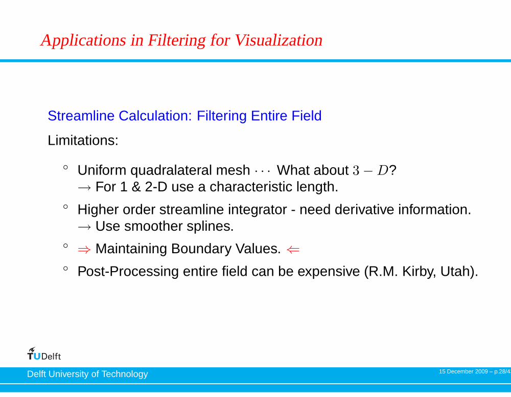
Applications in Filtering for Visualization
Streamline Calculation: Filtering Entire Field
Limitations:
Uniform quadralateral mesh · · · What about 3 −D?→ For 1 & 2-D use a characteristic length.
Higher order streamline integrator - need derivative information.→ Use smoother splines.
⇒ Maintaining Boundary Values. ⇐ Post-Processing entire field can be expensive (R.M. Kirby, Utah).
15 December 2009 – p.28/43

Delft University of Technology
(Old) Left Post-Processor
Ryan and Shu, MAA (2003)
u⋆(x) =
0X
j=−2p′
kX
l=0
u(l)i+j C(j, l, k, x)
where p′ = ⌈(3k + 1)/2⌉ ≤ 2k
and u⋆ ∈ P2k+1
C(j, l, k, x) =1
h
−kX
γ=−2k−1
c2(k+1),k+1γ
Z 12−(ξi+γ)
−12−(ξi+γ)
ψ(k+1) (η) (ξi + η + γ − j)l dy
For k = 1 :
K(x) =11
12ψ(2)(x+ 3) −
17
6ψ(2)(x+ 2) +
35
12ψ(2)(x+ 1)
15 December 2009 – p.29/43

Delft University of Technology
Old One-Sided Post-Processing: :ut + ux = 0, periodic BC
Problem 1: discontinuities are not eliminated (stair-stepping)Problem 2: the errors at the boundary can be worse than before
0 6.2832
10−12
10−10
10−8
10−6
10−4
10−2
20 el.
40 el.
80 el.
160 el.
Error Before Post−Processing
spatial domain0 6.2832
10−14
10−12
10−10
10−8
10−6
10−4
10−2
20 el.
40 el.
80 el.
160 el.
Error After Post−Processing (Old)
spatial domain
15 December 2009 – p.30/43

Delft University of Technology
New One-Sided Post-Processing: :ut + ux = 0, periodic BC
Problem 1: not all discontinuities are eliminated (stair-stepping)Problem 2: the errors at the boundary can be worse than before
0 6.2832
10−12
10−10
10−8
10−6
10−4
10−2
20 el.
40 el.
80 el.
160 el.
Error Before Post−Processing
spatial domain0 6.2832
10−14
10−12
10−10
10−8
10−6
10−4
10−2
20 el.
40 el.
80 el.
160 el.
Error After Post−Processing (Old)
spatial domain0 6.2832
10−14
10−12
10−10
10−8
10−6
10−4
10−2
20 el.
40 el.
80 el.
160 el.
Error After Post−Processing (New)
spatial domain
These problems can be solved through a new type of one-sidedpost-processing (following slides)
15 December 2009 – p.31/43

Delft University of Technology
New One-Sided Post-Processing
The discontinuities can be avoided by using kernel nodes that dependcontinuously on the evaluation point through the shift function λ(x):
u⋆h(x) =
2k∑
γ=0
cγ(x)
∫
I
ψ(k+1)h
(x− (λ(x) + γ)
︸ ︷︷ ︸
kernel node
)uh(x− x) dx.
van Slingerland, Ryan, & Vuik (2009).
15 December 2009 – p.32/43

Delft University of Technology
New One-Sided Post-Processing
The discontinuities can be avoided by using kernel nodes that dependcontinuously on the evaluation point through the shift function λ(x):
u⋆h(x) =
2k∑
γ=0
cγ(x)
∫
I
ψ(k+1)h
(x− (λ(x) + γ)
︸ ︷︷ ︸
kernel node
)uh(x− x) dx.
Three examples (the kernel nodes are indicated by the red circles):
λ(x) = −k
−2 −1 0 1 2
0
1
Symmetric kernel of order 2
x
Use in the domain interior.
λ(x) = k+12
0 1 2 3 4−3
−2
−1
0
1
2
3Right−sided kernel of order 2
x
Use at the left boundary
λ(x) = −0.5
−1.5 −0.5 0.5 1.5 2.5
0
1Partly right−sided kernel of order 2
x
Use near the left boundary
15 December 2009 – p.33/43

Delft University of Technology
New One-Sided Post-Processing
The discontinuities can be avoided by using kernel nodes that dependcontinuously on the evaluation point through the shift function λ(x):
u⋆h(x) =
2k∑
γ=0
cγ(x)
∫
I
ψ(k+1)h
(x− (λ(x) + γ)
︸ ︷︷ ︸
kernel node
)uh(x− x) dx.
−2k−(k+1)/2
−k
(k+1)/2Shift function λ(x)
xleft−sided
partly left−sided
symmetric
right−sided
partly right−sided
15 December 2009 – p.34/43
Delft University of Technology
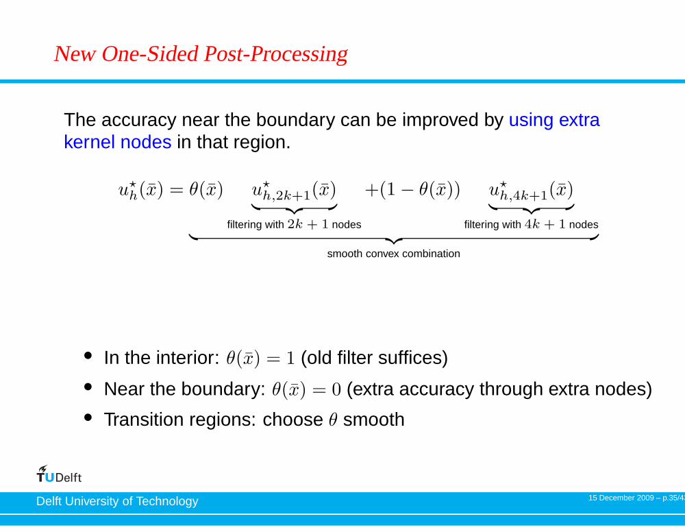
New One-Sided Post-Processing
The accuracy near the boundary can be improved by using extrakernel nodes in that region.
u⋆h(x) = θ(x) u⋆
h,2k+1(x)︸ ︷︷ ︸
filtering with 2k + 1 nodes
+(1 − θ(x)) u⋆h,4k+1(x)
︸ ︷︷ ︸
filtering with 4k + 1 nodes︸ ︷︷ ︸
smooth convex combination
• In the interior: θ(x) = 1 (old filter suffices)
• Near the boundary: θ(x) = 0 (extra accuracy through extra nodes)• Transition regions: choose θ smooth
15 December 2009 – p.35/43

Delft University of Technology
New One-Sided Post-Processing:ut + ux = 0, periodic BC
The new post-processor improves both the convergence rate and theabsolute value of the errors for a problem with a periodic BC
0 6.2832
10−12
10−10
10−8
10−6
10−4
10−2
20 el.
40 el.
80 el.
160 el.
Error Before Post−Processing
spatial domain0 6.2832
10−14
10−12
10−10
10−8
10−6
10−4
10−2
20 el.
40 el.
80 el.
160 el.
Error After Post−Processing (Old)
spatial domain0 6.2832
10−14
10−12
10−10
10−8
10−6
10−4
10−2
20 el.
40 el.
80 el.
160 el.
Error After Post−Processing (New)
spatial domain
15 December 2009 – p.36/43

Delft University of Technology
New One-Sided Post-Processing:ut + ux = 0, periodic BC
The new post-processor improves both the convergence rate and theabsolute value of the errors for a problem with a periodic BC
20 40 80 16010
−10
10−8
10−6
10−4
10−2
number of mesh elements
Convergence in the L2−error
Before Post−ProcessingAfter Post−Processing (Old)After Post−Processing (New)
20 40 80 16010
−10
10−8
10−6
10−4
10−2
number of mesh elements
Convergence in the L∞−error
Before Post−ProcessingAfter Post−Processing (Old)After Post−Processing (New)
15 December 2009 – p.37/43

Delft University of Technology
New One-Sided Post-Processing:ut + ux = 0, periodic BC
The new post-processor improves both the convergence rate and theabsolute value of the errors for a problem with a periodic BC
Before After (Old) After (New)
mesh L2-error order L2-error order L2-error order
Polynomial Degree k = 2
20 2.683e-04 - 4.003e-03 - 1.301e-05 -
40 3.352e-05 3.00 2.108e-04 4.25 3.767e-07 5.11
80 4.190e-06 3.00 5.464e-06 5.27 1.056e-08 5.16
160 5.238e-07 3.00 1.254e-07 5.45 3.090e-10 5.10
Polynomial Degree k = 3
20 5.176e-06 - 1.304e-04 - 3.757e-07 -
40 3.236e-07 4.00 4.712e-06 4.79 6.634e-10 9.15
80 2.023e-08 4.00 3.406e-08 7.11 2.957e-12 7.81
160 1.264e-09 4.00 1.999e-10 7.41 1.287e-14 7.8415 December 2009 – p.38/43

Delft University of Technology
New One-Sided Post-Processing:ut + ux = 0, Dirichlet BC
The new post-processor improves both the convergence rate and theabsolute value of the errors for a problem with a Dirichlet BC
0 6.283210
−14
10−12
10−10
10−8
10−6
10−4
10−2
20 el.
40 el.
80 el.
160 el.
Error Before Post−Processing
spatial domain0 6.2832
10−14
10−12
10−10
10−8
10−6
10−4
10−2
20 el.
40 el.
80 el.
160 el.
Error After Post−Processing (New)
spatial domain
15 December 2009 – p.39/43

Delft University of Technology
New One-Sided Post-Processing:ut + ux = 0, Dirichlet BC
The new post-processor improves both the convergence rate and theabsolute value of the errors for a problem with a Dirichlet BC
Before After (Old) After (New)
mesh L2-error order L2-error order L2-error order
Polynomial Degree k = 2
20 2.681e-04 - 4.003e-03 - 6.984e-06 -
40 3.352e-05 3.00 2.108e-04 4.25 1.850e-07 5.24
80 4.190e-06 3.00 5.464e-06 5.27 4.798e-09 5.27
160 5.238e-07 3.00 1.254e-07 5.45 1.498e-10 5.00
Polynomial Degree k = 3
20 5.176e-06 - 1.304e-04 - 3.751e-07 -
40 3.236e-07 4.00 4.712e-06 4.79 6.396e-10 9.20
80 2.023e-08 4.00 3.406e-08 7.11 2.867e-12 7.80
160 1.264e-09 4.00 1.999e-10 7.41 3.079e-14 6.5415 December 2009 – p.40/43

Delft University of Technology
New One-Sided Post-Processing:ut + aux = 0, a discontinuous
For this problem with two stationary shocks, the post-processorrequires a sufficiently fine mesh
−1 110
−10
10−8
10−6
10−4
10−2
100
102
20 el.
40 el.
80 el.
160 el.
Error Before Post−Processing
spatial domain−1 1
10−10
10−8
10−6
10−4
10−2
100
102
20 el.
40 el.
80 el.
160 el.
Error After Post−Processing (New)
spatial domain
15 December 2009 – p.41/43

Delft University of Technology
New One-Sided Post-Processing:ut + aux = 0, a discontinuous
For this problem with two stationary shocks, the post-processorrequires a sufficiently fine mesh
Before After (Old) After (New)
mesh L2-error order L2-error order L2-error order
Polynomial Degree k = 2
20 3.646e-02 - 6.808e+00 - 5.709e-01 -
40 2.052e-03 4.15 1.672e-01 5.35 1.249e-03 8.84
80 2.173e-04 3.24 6.027e-03 4.79 4.166e-05 4.91
160 2.682e-05 3.02 8.414e-05 6.16 1.181e-06 5.14
Polynomial Degree k = 3
20 1.085e-03 - 3.579e+00 - 2.270e-01 -
40 6.602e-05 4.04 1.865e-02 7.58 2.640e-03 6.43
80 4.132e-06 4.00 6.502e-04 4.84 5.205e-06 8.99
160 2.584e-07 4.00 2.623e-06 7.95 4.670e-09 10.1215 December 2009 – p.42/43

Delft University of Technology
Summary
Using B-splines allows us to induce smoothness on the DG field and enhanceaccuracy.
We can obtain this improvement from order k+1 to order 2k+1 for smoothly varyingmeshes as well as derivatives of the DG solution.
Recent extensions allow us to have the improvement in accuracy near theboundaries as well.• The kernel is adjusted according to the point we would like to post-process.• Near the boundary, we use more kernel nodes.
We can use this post-processing technique as a visualisation tool to maintain moreaccurate streamlines.
Acknowledgments: This research is supported by the U.S. Air Force Office of ScientificResearch under grant number FA8655-09-1-3055.
15 December 2009 – p.43/43