ACCT: 742-Advanced Auditing

SAS 56-Analytical Procedures (AU 329)

Regression Analysis and Other Analytical Procedures

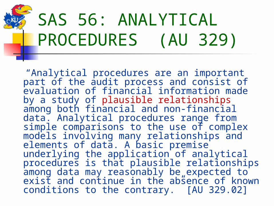
SAS 56: ANALYTICAL PROCEDURES (AU 329)

“Analytical procedures are an important part of the audit process and consist of evaluation of financial information made by a study of plausible relationships among both financial and non-financial data. Analytical procedures range from simple comparisons to the use of complex models involving many relationships and elements of data. A basic premise underlying the application of analytical procedures is that plausible relationships among data may reasonably be expected to exist and continue in the absence of known conditions to the contrary.” [AU 329.02]

Analytical procedures are used for the following purposes:

To assist the auditor in planning the nature, timing, and extent of other auditing procedures

As a substantive test to obtain evidential matter about particular assertions related to account balances or classes of transactions

As an overall review of the financial information in the final review stage of the audit

Timing and Purposes of Analytical Procedures-Planning Phase

Planning Phase(Required)Purpose

Understand client’sindustry and business Primary purpose

Assess going concern Secondary purpose

Indicate possible misstatements(attention directing) Primary purpose

Reduce detailed tests Secondary purpose

Timing and Purposes of Analytical Procedures-Testing Phase

Testing Phase(Recommended)Purpose

Understand client’sindustry and business

Assess going concern

Indicate possible misstatements(attention directing) Secondary purpose

Reduce detailed tests Primary purpose

Timing and Purposes of Analytical Procedures-Completion Phase

Completion Phase(Required)Purpose

Understand client’sindustry and business

Assess going concern Secondary purpose

Indicate possible misstatements(attention directing) Primary purpose

Reduce detailed tests

Five Types of Analytical Procedures

1. Compare client and industry data.2. Compare client data with similar

prior period data.3. Compare client data with client-

determined expected results.4. Compare client data with auditor-

determined expected results.5. Compare client data with expected

results, using non-financial data.

Some Specific Examples of Analytical Procedures

Ratio Analysis (Financial and Non-financial data) Common-Size Statements Trend Analysis Regression Analysis

Time Series Regression Cross-Sectional Regression

Discriminant Analysis Bankruptcy Models (Altman Z-factor)

Digital Analysis Intelligent Agents and Expert Systems

Altman Z-factor

Z = 1.2*X1 + 1.4*X2 + 3.3*X3 + 0.6*X4 + 1.0*X5

Z = discriminant or credit score

X1 = (working capital)/(total assets)

X2 = (retained earnings)/(total assets)

X3 = (earnings before interest and taxes)/(total assets)

X4 = (market value of equity)/(book value of total debt)

X5 = sales/(total assets)Z < 1.81: Company will go bankrupt within a year or two.2.675 > Z>1.81: Company will probably go bankrupt, but

there is a chance it will not.2.676 <Z< 2.99: Company will probably not go bankrupt, but

there is a chance it will.Z > 2.99: Company will not go bankrupt.

Altman Z-factor CalculationUse this website for a company's data: http://www.sec.gov/edgar.shtmlUse 10-K from SEC and stock price for the day from http://finance.yahoo.com/You may have to go to Google to search for the sicker symbol of your company

In millions except stock price

QualComm Inc. (QCOM)

Delta Ailines (DAL)

AAPL (Apple Computers)

  2009 2009 2009Stock Price (March 22, 2010)

$ 40.28

$ 13.07

$ 224.72

Number of Common Shares 1,674

794.873058 899.804500

Current Assets 13,574

7,741

36,265

Current Liabilites 2,948 9,797.00

19,282

Working Capital 10,626 (2,056) 16,983

Total Assets 28,903

43,539

53,851

MValue of Equity 67,429

10,389

$ 202,204.07

BV of Total Debt 7,550 43,294

26,019

Retained Earnings 11,792

(10,019)

19,538

EBIT 1,052 (1,581) 7,984

Sales 2,670 28,063

36,537

Z-factor 6.58 0.29 6.72

Regression Analysis Regression analysis is a statistical technique

used to describe the relationship between the account being audited and other possible predictive factors.

Regression analysis helps a. Determine whether there is a relationship between

the dependent and independent variablesb. Determine whether a “significant difference” has

occurred Simple Linear Regression (Time-series &

Cross-Sectional Analysis) Multiple Regression (Time-series & Cross-

Sectional Analysis)

Regression Analysis: Data Requirements

Accuracy and honesty in recording data

Accounting transactions should be properly accrued Data should be adjusted for economies of

scale or learning effects. Changes in the nature of production

process should be properly taken into consideration.

Variable level of activity is required.

Some Examples of Regression Analysis Applications

Monthly sales based on cost of sales and selling expense

Airline and truck company fuel expense based on miles driven and fuel cost per gallon

Maintenance expense based on production levels Overhead cost based on machine hours and labor

hours used Inventory at each location of a retail company

based on store sales, store square footage, regional economic data, and type of store location

Linear Regression Model

yi = a + bxi + i

yi = dependent variable at time ‘i’ or location ‘i’

xi = independent variable at time ‘i’ or location ‘i’

i = Error term that incorporates (1) the effects of omitted variables, and (2) model errors caused by nonlinear relationships between x and y.

‘a’ and ‘b’ are estimated by minimizing the sum of the squared terms (Ordinary Least Squares, OLS, technique)

Minimize: (i)2= (yi – a - bxi)2

Regression Line: y = a + bxScatter Graph

150

200

250

300

350

400

150 200 250 300

Independent Variable X

Dep

en

den

t V

ari

ab

le Y

i = (yi-y)

Minimize variance (i)2

a

Assumptions

Linear relationship between the dependent variable and the independent variable(s).

E(i) = 0, i.e., i = 0.

Variance of i is constant for all t, and does not depend on the independent variables.

Covariance(i, j) = 0, for all i, j where i j.

The independent variables are uncorrelated.

i ~ N(0, ).

E(i) = 0, i.e., i = 0.

X Variable 1 Residual Plot

-40-30-20-10

010203040506070

150 200 250 300

X Variable 1

Resid

uals i

i = 0

Variance of i is constant for all i

X Variable 1 Residual Plot

-40-30-20-10

010203040506070

150 200 250 300

X Variable 1

Resid

uals

Four Criteria For Evaluating Regression Results

Plausibility of relationship between the dependent variable and the independent variables.

Goodness of fit measured by R2 (Coefficient of determination) and F statistic.

Confidence placed on the parameters of the regression model.

Specification Tests – Critical assumptions have been met.

Goodness of fit Measured by Coefficient of Determination

R2 (Coefficient of Determination) represents the percentage of variance explained in the dependent variable through the independent variables.

Value: 1>R2>0

If R2 = 0.85, it means 85% of variance is explained by the independent variable(s)

Significance of the Coefficients

Y = a + bx Is ‘a’ different from zero? Determines if there is a

constant term. Is ‘b’ different from zero? Determines if there is a

linear relationship.

We use t-statistics to test for their significance

ta = (a – 0)/sa, sa is the standard deviation of ‘a’

tb = (a – 0)/sb , sb is the standard deviation for ‘b’

As a rule of thumb, for a large sample size, if t is greater than 2 then we consider the coefficient to be different from zero.

Standard Error of the Regression and Standard

deviations of a and b

The standard error of the regression

where n is the number of data points and k is number of unknown parameters in the model.

The standard deviation of b, the coefficient of the independent variable:

2i

e

(y from data y from regression line)s =

(n - k)

eb 2

i

ss =

(x x mean from the data)

Standard Deviation of the parameter a

The standard error of the constant term, a:

2

a e 2i

1 (x mean from data)s = s .

n (x x mean from data)

Prediction: yf from regression line = a + bxf. The standard error Sf for yf is given by:

The t statistic for the test of significance is:

Predictions from the Regression Equation

f ff

f

y from regression line y from datat =

s

2f

f e 2i

(X X)1S = S . 1

n (X X)

95% Confidence Intervals

yf

Confidence interval for coefficient a:

= [ a ± t.95 sa]

Confidence interval for coefficient b:

= [ b ± t.95 sb]

Confidence interval for the predicted value :

= [ ± t.95 sf]

yf