Embed Size (px)
Citation preview

Accretion Disks and the Formation of Stellar Systems
by
Kaitlin Michelle Kratter
A thesis submitted in conformity with the requirementsfor the degree of Doctor of Philosophy
Graduate Department of Astronomy and AstrophysicsUniversity of Toronto
Copyright c! 2010 by Kaitlin Michelle Kratter

Abstract
Accretion Disks and the Formation of Stellar Systems
Kaitlin Michelle Kratter
Doctor of Philosophy
Graduate Department of Astronomy and Astrophysics
University of Toronto
2010
In this thesis, we examine the role of accretion disks in the formation of stellar sys-
tems, focusing on young massive disks which regulate the flow of material from the parent
molecular core down to the star. We study the evolution of disks with high infall rates
that develop strong gravitational instabilities. We begin in chapter 1 with a review of the
observations and theory which underpin models for the earliest phases of star formation
and provide a brief review of basic accretion disk physics, and the numerical methods
that we employ. In chapter 2 we outline the current models of binary and multiple star
formation, and review their successes and shortcomings from a theoretical and observa-
tional perspective. In chapter 3 we begin with a relatively simple analytic model for disks
around young, high mass stars, showing that instability in these disks may be responsible
for the higher multiplicity fraction of massive stars, and perhaps the upper mass to which
they grow. We extend these models in chapter 4 to explore the properties of disks and
the formation of binary companions across a broad range of stellar masses. In particular,
we model the role of global and local mechanisms for angular momentum transport in
regulating the relative masses of disks and stars. We follow the evolution of these disks
throughout the main accretion phase of the system, and predict the trajectory of disks
through parameter space. We follow up on the predictions made in our analytic models
with a series of high resolution, global numerical experiments in chapter 5. Here we
propose and test a new parameterization for describing rapidly accreting, gravitationally
unstable disks. We find that disk properties and system multiplicity can be mapped out
ii

well in this parameter space. Finally, in chapter 6, we address whether our studies of
unstable disks are relevant to recently detected massive planets on wide orbits around
their central stars.
iii

Dedication
To my mother, for her love, support, and confidence
To my father, who always told me ‘do something interesting, like astrophysics’
To my brother, for setting the bar all along
And to Grandpa Leo, who would have been proudest of all
iv

Acknowledgements
This thesis was funded jointly by the Connaught Doctoral Student Scholarship, the Uni-versity of Toronto and an Ontario Graduate Scholarship.
First, I would like to thank my thesis advisor, Chris Matzner, for his support, insight,and enthusiasm over the last five years, and for suggesting a first year project that turnedout to be far more interesting than either of us imagined.
Secondly, I would like to acknowledge the contributions of my co-authors, withoutwhom I could not have completed these projects. I am grateful to Mark Krumholz forapproaching me at a conference when I was just starting out, and for his continued guid-ance. I would like to thank Ruth Murray-Clay and Andrew Youdin for their importantcontributions to the final chapter of this thesis. I am also grateful to Richard Klein forhis thoughtful comments, and for providing the numerical code used in chapter five.
I would also like to acknowledge the faculty and post docs in the department, CITA,and elsewhere for fruitful discussions, and technical assistance. In particular JonathanDursi for lending his extensive computational expertise and crucial moral support. I amalso indebted to my first reearch advisor, Charles Liu, for throwing me in to the deepend, in a good way.
Finally, thanks to all the friends who got me here, and kept me going. Especially:
Darren, for the confidence to pursue something hard
Alexis, Andy, Aleks, and KB, for reminding me how to have fun
Bart, Julia, Derek, and Oasis, for their crucial contributions to Chapter 7 of this thesis
Lawrence, for setting all the right examples, and showing inconceivable tolerance to anover-eager first year
Sha-non, Aroy, Nicky, and Pena, for the company, 12th floor pride, and Timmy’s
And Andrew, for all the catches, the unfrozen water, the snowy drives, and the warmmeals. And most of all, for holding my hand.
v

Contents
1 Introduction 1
1.1 Motivation . . . . . . . . . . . . . . . . . . . . . . . . . . . . . . . . . . . 1
1.2 Disks and the Earliest Phases of Star Formation . . . . . . . . . . . . . 2
1.3 Disk Physics: Mechanisms for Angular Momentum Transport . . . . . . 6
1.4 Numerical Techniques . . . . . . . . . . . . . . . . . . . . . . . . . . . . 20
2 Observational Connections 25
2.1 Introduction . . . . . . . . . . . . . . . . . . . . . . . . . . . . . . . . . . 25
2.2 Standard Theories of Binary and Multiple Star Formation . . . . . . . . 26
2.3 Observational Tests of Theoretical Models . . . . . . . . . . . . . . . . . 30
2.4 Conclusions . . . . . . . . . . . . . . . . . . . . . . . . . . . . . . . . . . 34
3 Disks in the Formation of Massive Stars 35
3.1 Introduction . . . . . . . . . . . . . . . . . . . . . . . . . . . . . . . . . . 35
3.2 Disk Fragmentation . . . . . . . . . . . . . . . . . . . . . . . . . . . . . . 36
3.3 Core Accretion . . . . . . . . . . . . . . . . . . . . . . . . . . . . . . . . 46
3.4 Fragmentation of Core-Collapse Disks . . . . . . . . . . . . . . . . . . . . 52
3.5 Consequences of Instability . . . . . . . . . . . . . . . . . . . . . . . . . . 58
3.6 Discussion . . . . . . . . . . . . . . . . . . . . . . . . . . . . . . . . . . . 63
3.7 Appendix . . . . . . . . . . . . . . . . . . . . . . . . . . . . . . . . . . . 65
4 Global Models of Young, Massive Protostellar Disks 70
4.1 Introduction . . . . . . . . . . . . . . . . . . . . . . . . . . . . . . . . . . 70
4.2 Infall onto Disks . . . . . . . . . . . . . . . . . . . . . . . . . . . . . . . . 72
4.3 Dynamics of the disk . . . . . . . . . . . . . . . . . . . . . . . . . . . . . 76
4.4 Expected Trends . . . . . . . . . . . . . . . . . . . . . . . . . . . . . . . 89
vi

4.5 Results . . . . . . . . . . . . . . . . . . . . . . . . . . . . . . . . . . . . . 92
4.6 Observable Predictions . . . . . . . . . . . . . . . . . . . . . . . . . . . . 105
4.7 Conclusions . . . . . . . . . . . . . . . . . . . . . . . . . . . . . . . . . . 107
5 Numerical Models 111
5.1 Introduction . . . . . . . . . . . . . . . . . . . . . . . . . . . . . . . . . . 111
5.2 A New Parameter Space for Studying Accretion . . . . . . . . . . . . . . 112
5.3 Numerical Methodology . . . . . . . . . . . . . . . . . . . . . . . . . . . 115
5.4 Disk properties in terms of the accretion parameters . . . . . . . . . . . . 121
5.5 Results . . . . . . . . . . . . . . . . . . . . . . . . . . . . . . . . . . . . . 124
5.6 The formation of binaries and multiples . . . . . . . . . . . . . . . . . . 139
5.7 Caveats and Numerical E!ects . . . . . . . . . . . . . . . . . . . . . . . 143
5.8 Comparison to Previous Studies . . . . . . . . . . . . . . . . . . . . . . . 149
5.9 Discussion . . . . . . . . . . . . . . . . . . . . . . . . . . . . . . . . . . . 152
6 GI and Planets 154
6.1 Introduction . . . . . . . . . . . . . . . . . . . . . . . . . . . . . . . . . . 154
6.2 The HR 8799 system . . . . . . . . . . . . . . . . . . . . . . . . . . . . . 157
6.3 Ideal Conditions for GI-driven Fragment Formation . . . . . . . . . . . . 157
6.4 Minimum fragment masses and separations . . . . . . . . . . . . . . . . . 159
6.5 Growth of fragments after formation . . . . . . . . . . . . . . . . . . . . 168
6.6 GI planet formation in the context of star formation . . . . . . . . . . . . 174
6.7 Migration in a multi-planet system . . . . . . . . . . . . . . . . . . . . . 176
6.8 Current Observational Constraints . . . . . . . . . . . . . . . . . . . . . 180
6.9 Summary . . . . . . . . . . . . . . . . . . . . . . . . . . . . . . . . . . . 181
6.10 Appendix A. Cooling and Fragmentation in Irradiated disks . . . . . . . 182
6.11 Appendix B. Temperature due to Viscous Heating . . . . . . . . . . . . . 185
Bibliography 186
vii

List of Tables
3.1 Definitions of subscripts. . . . . . . . . . . . . . . . . . . . . . . . . . . . 39
3.2 Estimates of angular momentum of observed disks in figure 3.3 and cor-
responding references. Angular momentum estimates are computed from
the observed velocity gradient over the extent of the disk. Estimates are
only made for data points that showed a clear velocity gradient associated
with a disk or torus. . . . . . . . . . . . . . . . . . . . . . . . . . . . . . 43
3.3 Observational data points in figure 3.3 and corresponding references. . . 56
3.4 Values of "j2#1/2/(R"!2#1/2) in our model for turbulent angular momentum. 67
4.1 Fiducial parameters for disk models for low and high mass stars, and the
accompanying ranges explored. . . . . . . . . . . . . . . . . . . . . . . . 93
5.1 Each run is labelled by ", ", multiplicity outcome, the final value of the
disk-to-star(s) mass ratio,µ and the final resolution, #n. Values of " are
quoted in units of 10!2. For fragmenting runs the disk resolution #f , Q2D
(equation 5.29) and µf at the time of fragmentation are listed as well. S
runs are single objects with no physical fragmentation. B’s are binaries
which form two distinct objects each with a disk, and M are those with
three or more stars which survive for many orbits. * indicates runs which
are not su#ciently well resolved at the time of fragmentation to make
meaningful measures of µf , and Q. . . . . . . . . . . . . . . . . . . . . . 125
5.2 Non-fragmenting runs (numbers as from table 5.1). We list values for the
characteristic predicted value of Toomre’s Q, Qd (equation 5.23), as well
as the measured disk minimum, Q2D equation (5.29). We also list the
slope of the surface density profile, k! averaged over several disk orbits,
the final resolutions, and Rd at the end of the run (equation 5.21) . . . . 127
viii

List of Figures
1.1 Exchange of fluid parcels in a plane shear flow as shown by Frank et al.
(2002). vz represents the average random velocity in the z direction at
which particles are exchanged and vx is the background shear velocity. d
is the characteristic lengthscale of the interaction. In this example, shear
viscosity tries to smooth out the velocity gradient. . . . . . . . . . . . . . 9
1.2 Small section of an accretion disk in the shearing box approximation. The
disk is threaded by vertical field lines. A fluid parcel perturbed outwards
will continue to be moved outwards as tension in the magnetic field line
transfers angular momentum to the gas. . . . . . . . . . . . . . . . . . . 13
1.3 Trailing spiral wave induces positive correlations between g! and gr follow-
ing Figure 1 of Lynden-Bell & Kalnajs (1972). For example, the arrows in
the lower right quadrant indicate that material inside the arm is acceler-
ated in the positive $ and r directions, while material outside of the arm
is accelerated in the negative $ and r directions. . . . . . . . . . . . . . . 17
3.1 The fragmentation radius (in AU) is shown for a range of central star
masses and accretion times. Also shown is the star formation time in the
core model (dotted lines, for 0.3 < $cl < 3 g cm!2) and the region a!ected
by dust sublimation in the infall envelope (filled region), where our model
does not hold. The sharp kink in the lines of constant radius is due to a
drop in opacity for disk temperatures above about 1050K. . . . . . . . . 44
ix

3.2 Angular momentum and disk fragmentation. The critical value of angular
momentum, labeled as log10(jcrit), is plotted as bold curves for a range of
stellar masses and formation times, tacc = 2M"/(M"d). Dashed lines show
our predicted angular momentum for the McKee & Tan (2003) core model
(% = 0.5, k# = 1.5). As discussed in §4.3.4, this is also an approximate
upper limit to j given M" and tacc. Disks tend to fragment except in the
upper, dark filled region. In the lower, light filled region, envelope dust
grains sublimate within Rd; our model is not secure here. Dotted lines
delimit core model formation times for 0.3 < $cl < 3 g cm!2. . . . . . . . 45
3.3 Relevant radii. The characteristic disk radius predicted by (fiducial) core
accretion is accompanied by a shaded band illustrating our (Maxwellian)
model for its dispersion. The largest stable radius is plotted for compar-
ison; this is accompanied by the contributions from pure irradiation (no
viscous heat) and pure viscosity (no irradiation). The turnover of Rcrit
above $ 20M" is due to the scaling of ZAMS mass and luminosity. The
references for the observational points are listed in table (3.3). Circles
represent objects that may best be described as cores, whereas diamonds
represent those objects whose disks are well resolved. Squares indicate ob-
jects for which it is unclear whether they are rotating, infalling, or both;
see §3.5.2 for discussion. . . . . . . . . . . . . . . . . . . . . . . . . . . . 55
3.4 E!ect of varying the star formation e#ciency % in the fiducial core collapse
model. Dashed lines: critical disk radius Rd,crit for fragmentation; solid
lines: expected disk extent Rd. Intersections are as marked. . . . . . . . 57
3.5 Growth of disk and critical radius with the mass of a protostar accret-
ing toward 30M" in the fiducial core collapse model. In addition to the
expected disk radius, we show the splashdown radius of the inner infall
streamline, calculated assuming % = 0.5. . . . . . . . . . . . . . . . . . . 59
3.6 Our estimate of the initial fragment mass, compared to the gap opening
mass and isolation mass, at the end of accretion in the fiducial core collapse
model. We truncate the calculation where dust sublimation in the envelope
makes the critical radius determination uncertain. . . . . . . . . . . . . . 61
3.7 Values of "j2#1/2/(R"!2#1/2) evaluated for turbulence with line width-size
exponent & and three relevant density profiles. For hydrostatic turbulent
cores, ' % r!2(1!$). . . . . . . . . . . . . . . . . . . . . . . . . . . . . . . 68
x

4.1 Contours of the viscosity parameter log((GI) due to gravitational instabil-
ities (eq. 4.15); white squares are contour labels. Results from numerical
simulations are marked with circles, diamonds, and triangles. Circles show
simulations with adiabatic equations of state (Laughlin & Rozyczka, 1996),
diamonds show simulations with an imposed cooling rate that reach steady
state (Lodato & Rice, 2004, 2005), and triangles show the maximum (GI
achieved in simulations with imposed cooling that probe the fragmentation
boundary (Gammie, 2001; Rice et al., 2003; Lodato & Rice, 2004, 2005).
Note that the point at µ = 0 corresponds to the purely local simulation of
Gammie (2001). The Q = 1 boundary is marked with a dashed line. . . . 82
4.2 Contours of the dimensionless accretion rate from the disk onto the star
(M#/Md%) from all transport components of our model. The lowest con-
tour level is 10!4.8, and subsequent contours increase by 0.3 dex. The
e!ect of each transport mechanism is apparent in the curvature of the
contours. At Q < 1.3 the horizontal “tongue” outlines the region in which
short wavelength instability dominates accretion. The more vertical slope
of the contours at lower µ and Q > 1.3 shows the dominance of the long
wavelength instability. The MRI causes a mild kink in the contours across
the Q = 2 boundary and is more dominant at higher disk masses due to
our assumption of a constant (: equation [4.13] illustrates that a constant
( will cause higher accretion rates at higher values of µ. . . . . . . . . . 83
4.3 A simplified schematic of the decision tree in the code. The primitive
variables, Md, M#, and Jd, together with the core model, Min(t) and Jin(t),
allow for the determination of all disk parameters at each time step. Note
that cs, Q, and M are solved for simultaneously. Once the self-consistent
state is found, the values of Q and µ determine whether either the binary
or fragmentation regime has been reached. See §4.3.7 for a description of
the elements in detail. . . . . . . . . . . . . . . . . . . . . . . . . . . . . 90
xi

4.4 Evolutionary tracks in the Q, µ plane of a 1M"(left) and 15 M" (right)
final star-disk system overlayed on the contours of our accretion model
(contour spacing is identical to Figure 4.2). The white arrows superposed
on the tracks show the direction of evolution in time. The low mass star re-
mains stable against fragmentation throughout its history, while the more
massive star undergoes fragmentation and more violent variation in disk
mass. The jump a the end of accretion in the 15 M" system is due to the
switch in the irradiation calculation. . . . . . . . . . . . . . . . . . . . . 95
4.5 Contours of Q over the accretion history of a range of masses for the
fiducial sequence. Masses listed on the y-axis are for the total star-plus-
disk system final mass – because the models halt at 2 Myr, some mass
does remain in the disk. Contours are spaced by 0.3 dex. At low final
stellar masses, disks remain stable against the local instability throughout
accretion. At higher masses, all undergo a phase of fragmentation. One
can see three distinct phases in the evolution as described in §4.5. Disks
start out stable, subsequently develop spiral structure as the disk mass
grows and become unstable to fragmentation for su#ciently high masses.
As accretion from the core halts, they drain onto the star and once again
become stable. . . . . . . . . . . . . . . . . . . . . . . . . . . . . . . . . . 97
4.6 Contours showing the evolution of µ = MdMd+M!
for the fiducial sequence.
Each contour shows an increase of 0.05 in µ. Again one can see the division
into three regimes: low mass disks at early times, higher mass, unstable
disks that may form binaries during peak accretion times, and low mass
disks that drain following the cessation of infall. Systems destined to
accrete up to $ 70M" or more experience two epochs of binary formation
in our model. In these systems the accretion from the core exceeds the
maximum disk accretion rate very early, causing the disk mass to build up
quickly. . . . . . . . . . . . . . . . . . . . . . . . . . . . . . . . . . . . . 98
xii

4.7 Comparison of disk radius over the evolution of a 20 M" star-disk system
in four cases: the KM06 analytic calculation, the circularization radius
of the currently accreting material, and two realizations of the numerical
model. The analytic case overestimates the expected radius at early times
because it does not allow for cancellation of vector angular momentum.
Similarly the circularization radius is an overestimate because the disk
has no “memory” of di!erently oriented j. At later times, the circulariza-
tion radius approaches the standard radius calculation for that realization
(thick black line) demonstrating the concentration of turbulent power at
large scales. . . . . . . . . . . . . . . . . . . . . . . . . . . . . . . . . . . 99
4.8 Contours of Q showing the e!ect of initial core temperature Tc (left) and
$c (right) on the evolution of a 1 M" final star-disk system. Contour
spacing is 0.1 dex (except the lowest two contours which are spaced by .05
dex). Increasing $c tends to marginally destabilize the disk, while higher
temperatures stabilize the disk. We exclude temperatures too high for the
2M" core to collapse given its initial density, i.e., those above 40 K. . . . 101
4.9 Contours in µ illustrating the influence of varying (MRI (top) and the
braking index, bj (bottom) for a star-disk system of final mass 15M", the
lowest mass at which a binary forms in our fiducial model. Contours of µ
are spaced by 0.05. The upper plot shows the e!ect of varying (MRI from
10!2.5 & 10!1.5. While the change has little e!ect on the evolution of Q,
the disk fraction µ decreases with increasing (MRI. As a result, the mass
at which binary formation begins is pushed to higher masses. The lower
plot shows the e!ect of varying the braking index bj. An increase of bj
lowers the disk angular momentum, reducing the disk mass and inhibiting
binary formation. Note that the variation in disk mass is only $ 10%. . . 103
5.1 Two examples of single, binary, and multiple systems. The resolution
across each panel is 328x328 grid cells. The single runs are " = 2.9, " =
0.018 (top), " = 1.6, " =0 .009 (bottom). The binaries are " = 4.2, " =
0.014 (top), " = 23.4, " =0 .008, (bottom). The multiples are " = 3.0, " =
0.016 (top), " = 2.4, " =0 .01 (bottom). Black circles with plus signs
indicate the locations of sink particles. These correspond to runs 5, 1, 9,
16, 7, and 4 respectively. . . . . . . . . . . . . . . . . . . . . . . . . . . . 120
xiii

5.2 Distribution of runs in "&" parameter space. The single stars are confined
to the low " region of parameters space, although increasing " has a small
stabilizing e!ect near the transition around " = 2 due to the increasing
ability of the disk to store mass at higher values of ". The dotted line
shows the division between single and fragmenting disks: " = "2.5/850. As
" increases disks fragment to form multiple systems. At even higher values
of " disks fragment to make binaries. We discuss the distinction between
di!erent types of multiples in §5.6. The shaded region of parameter space
shows where isothermal cores no longer collapse due to the extra support
from rotation. . . . . . . . . . . . . . . . . . . . . . . . . . . . . . . . . 126
5.3 Top: Qav in a disk with " = 2.9, " = 0.018. The current disk radius,
Rk,in is shown as well. Bottom: Log(Q2D) (equation 5.29) in the same
disk. While the azimuthally averaged quantity changes only moderately
over the extent of the disk, the full two-dimensional quantity varies widely
at a given radius. Q is calculated using ) derived from the gravitational
potential, which generates the artifacts observed at the edges of the disk.
Here and in all figures, we use *x to signify the resolution. . . . . . . . . 128
5.4 Steady-state and pre-fragmentation values of Q and µ for single stars and
fragmenting disks respectively. We use the minimum of Q2D as described
in §5.5.1. Symbols indicate the morphological outcome. Note that the
non-fragmenting disks (large triangles) have the highest value of µ for
a given Q. Contours show the predicted scaleheight as a function of Q
and µ. It is clear that the single disks lie at systematically higher scale
heights. We have assumed k! = 3/2 in calculating scaleheight contours as
a function of Q and µ. . . . . . . . . . . . . . . . . . . . . . . . . . . . . 130
5.5 At right " vs µ with the fit in equation (5.31) overplotted. At left, Qdµ vs
" with the scaling Q % "!1/3 overplotted. Runs, 16, 17, 18 are omitted as
the low resolution at the time of fragmentation makes measurements of µ
and therefore Qd unreliable. . . . . . . . . . . . . . . . . . . . . . . . . . 131
xiv

5.6 Normalized density profiles for the single-star disks. Profiles are azimuthal
averages of surface densities over the final $ 3 disk orbital periods. We
find that while the inner regions are reasonably approximated by power law
slopes, the slope steepens towards the disk edge. For comparison, slopes
of k! = 1, 1.5, and 2 are plotted as well. Runs are labelled according to
their values in table 5.1. . . . . . . . . . . . . . . . . . . . . . . . . . . . 132
5.7 Azimuthal averages of di!erent components of torque expressed as an ef-
fective ( (equation 5.34) for run #8. The straight line, (d (equation 5.32)
is plotted for comparison. The agreement between the analytic value of
(d and the combined contribution from the other components is best near
the expected disk radius Rk,in. . . . . . . . . . . . . . . . . . . . . . . . . 133
5.8 Cuts along the vertical axis and disk midplane of the vertical velocity,
normalized to the disk sound speed. Clearly most of the vertical motions
in the disk are transonic, although at the edges of the disk the velocities
exceed M $ 1. . . . . . . . . . . . . . . . . . . . . . . . . . . . . . . . . 136
5.9 Top: the x and y components of the velocity of the central star normalized
by the disk sound speed for run #14. Bottom: the combined orbital
velocity of the star normalized to the sound speed. The velocity o!set
grows until the disk fragments. . . . . . . . . . . . . . . . . . . . . . . . . 138
5.10 Examples of the log of the disk surface density and corresponding fourier
mode strengths when an m = 2 mode dominates (top, run #13) and when
an m = 1 mode dominates bottom (run #8), both within about one disk
orbit of fragmentation. At bottom one can clearly see both the overall
asymmetry and the pronounced m = 2 spiral. Note that run #8 shows a
similar growth pattern to Fig. 5.9, while the top image, run #13 does not. 140
5.11 Density slices showing vertical structure in a single and binary disk. The
top plot is a single star with " = 1.6, " =0 .09, while the bottom is
a fragmenting binary system with " = 24.3, " = 0.008. The extended
material in the binary system is generated by a combination of large scale
circumbinary torques and the infalling material. Colorscale is logarithmic.
The box sizes are scaled to 1.5Rk,in in the plane of the disk. . . . . . . . . 144
xv

5.12 Correlation between #f and the infalling accretion rate for heated and non
heated runs with comparable ". Plus symbols indicate non-heated runs,
and the crosses are heated runs. The arrows and red crosses indicate the
position of the runs evaluated with respect to "core. Runs shown have
" values ranging from 0.006 to 0.009. The shaded region illustrates the
scaling #f % "!1. This scaling is related not only to the existence of a
critical value of µ, but also tied to the e!ect of resolution on fragmentation.146
5.13 At left: a snapshot of the standard resolution of run #16 shortly after
binary formation. At right, the same run at double the resolution. Be-
cause of the self-similar infall prescription, we show the runs at the same
numerical resolution, as time and resolution are interchangeable. In this
case the high-resolution run has taken twice the elapsed “time” to reach
this state. The two runs are morphologically similar and share expected
disk properties. . . . . . . . . . . . . . . . . . . . . . . . . . . . . . . . . 147
5.14 Trajectory of a Bonnor-Ebert sphere through " & " space. The two lines
show values of & = 0.02, 0.08 as defined in Matsumoto & Hanawa (2003).
Arrows indicate the direction of time evolution from t/t",0 = 0& 5. t",0 is
evaluated with respect to the central density, and arrows are labelled with
the fraction of the total Bonnor-Ebert mass which has collapsed up to this
point. The dotted line shows the fragmentation boundary from Figure 5.2. 151
6.1 The disk cooling time as a function of tempertature for di!erent opacity
laws at radii of 40 AU (dashed) and 100 AU (solid). The cooling time
is calculated assuming that Q = 1. The temperature independent (large
grain) opacity law is shown in red, while the ISM opacity law: ) % T 2
is shown in blue. The line thickness indicates the optical depth regime.
When lines drop below the critical cooling time (grey), disk fragmenta-
tion can occur. The bend in the ISM opacity curve indicates that in the
optically thick regime, the cooling time becomes constant as a function of
temperature. . . . . . . . . . . . . . . . . . . . . . . . . . . . . . . . . . 163
xvi

6.2 Fragmentation can only occur in the region of parameter space indicated
by the overlapping hashed regions for ISM opacities at radii of 100 AU.
The upper, shaded region (red) shows where Toomre’s parameter Q < 1.
The lower, shaded region (blue) indicates where tcool ' 3%!1. At radii less
than 70 AU, fragmentation is prohibited because the two regions no longer
overlap. That the boundaries of these regions are parallel lines reflects the
) % T 2 form of the ice-grain-dominated opacity at low temperatures. . . 165
6.3 Depiction of the current configuration of HR 8799 and formation con-
straints for realistic disk temperatures. We show the lowest expected irra-
diated disk temperatures (blue) and corresponding fragment masses (grey),
as a function of radius. The lower bound on both regimes (burgundy) is set
by the irradiation model described in §6.4.3, with M = 10!7M"/yr. The
upper boundary is set by the current luminosity of HR 8799, $ 5L". The
green dashed-dotted line shows the mass with disk temperatures of 10 K,
a lower limit provided by the cloud temperature. The vertical line shows
the critical fragmentation radius for the ISM opacity law; fragmentation
at smaller radii requires grain growth. Fragment masses are shown for
radii at which the irradiation temperatures are high enough to satisfy the
cooling time constraint of equation (6.17). At smaller radii, fragmentation
is possible at higher disk temperatures, but the resulting fragments have
correspondingly higher masses, and planet formation is not possible. . . 167
6.4 Contours of the ratio of planetary isolation mass to stellar mass as a func-
tion of Toomre’s Q and the disk aspect ratio H/r, illustrating that the
isolation mass is always large in unstable disks. For disks with higher Q’s
consistent with core accretion models, the isolation mass remains small.
The shaded region indicates where the isolation mass exceeds the stellar
mass. . . . . . . . . . . . . . . . . . . . . . . . . . . . . . . . . . . . . . 169
xvii

6.5 The gap starvation mass as a function of disk radius. We show curves
for several values for (, and indicate the planetary mass regime, and the
region in which disk fragmentation is likely. We use fS = 5, scaled to
simulation 2lJ of Jupiter formation in Lissauer et al. (2009) (labeled L09
in the figure). The radial scaling is derived assuming H/r % r2/7. For
the low viscosity case, we normalize the scale height to Jupiter at 5.2
AU in a 115 K disk for comparison with L09. For the higher viscosities,
we normalize the disk scale height to the lowest expected temperatures
(equation 6.20). For comparison we show the HR 8799 planets as black
circles. . . . . . . . . . . . . . . . . . . . . . . . . . . . . . . . . . . . . . 173
6.6 (Left) Known substellar companions (stars) and planets (plusses) as a
function of mass ratio and projected separation. The three objects in the
HR 8799 system are shown by pink circles, and a pink triangle denotes
the upper-limit mass ratio for Fomalhaut b based on the dynamical mass
estimate of Chiang et al. (2009). Grey squares indicate the gap regions.
Ongoing surveys are necessary to determine whether there is a continu-
ous distribution between Jupiter/Saturn (blue diamonds) and HR 8799,
or HR 8799 and brown dwarf companions. Planets around very low mass
primaries with M# = 0.02–0.1M" are marked by purple squares. These
systems have mass ratios more akin to the substellar companions than to
the remainder of the population of planets. Primary masses range from
M# = 0.02M"–1M" (black) and M# = 1M"–2.9M" (red) for substellar
companions and from M# = 0.1–0.4M" (purple) and M# = 0.4–4.5M"
(black) for planets. (Right) The same objects plotted as function of the
minimum fragment mass, Mfrag,min and critical radius, rcrit. We use equa-
tion (6.16) to calculate rcrit. For Mfrag,min, we apply equation (6.6) at radius
rcrit under the simplified assumption that the disk temperature is set by the
stellar luminosity: L/L" = (M#/M")3.5 for M# > 0.43M" and L % M2.3#
for lower-mass stars. The temperatures used to calculate fragment masses
are not allowed to dip below 20K. Masses below Mfrag,min are unlikely to
result from GI. . . . . . . . . . . . . . . . . . . . . . . . . . . . . . . . . 179
xviii

Chapter 1
Introduction
1.1 Motivation
The focus of this thesis is on understanding the role of accretion disks in the earliest
phases of star formation, with careful consideration of the di!erences between single
and multiple systems. In particular, we focus on the role of gravitational instabilities in
driving accretion and fragmentation in young, massive, protostellar disks.
In order to explore these questions we employ two complimentary techniques. On the
one hand, we use simplified semi-analytic models to tease out the important parameters
of the problems we explore. These simple models allow us to take into account di!erent
physical e!ects and explore a broad range of parameter space. This technique is key to
our ability to make general inferences about the behavior of accretion disks across the
entire stellar mass function. Of course this type of analysis is limited because we must
use somewhat crude approximations of complex phenomena: for example, we reduce
complex non-linear instabilities to a few algebraic definitions. And so to complement
these investigations, we also perform high resolution, targeted numerical experiments in-
formed by our simple models. This combined approach has provided insight into angular
momentum transport via gravitational instability, and in particular the saturation of the
instability in massive disks with ongoing mass accretion.
This work began as an investigation into the role of disks in the formation of massive
stars. We first used a quasi-steady state model to delineate the parameters of gravita-
tionally unstable disks around massive stars, showing that fragmentation was likely, and
that such disks might have much in common with AGN (chapter 3). Our initial inquiry
led to a much broader exploration of the role of massive accretion disks in the formation
1

Chapter 1. Introduction 2
of binaries and hierarchical multiples. We produced evolutionary tracks for non-steady
state, gravitationally unstable disks around stars across a broad mass range in order to
track the state of disks and system multiplicity throughout the embedded phase of star
formation (chapter 4). To check our prescription for accretion in self-gravitating disks,
we conducted numerical experiments using a new parameterization for rapidly accreting
disks, which appear to be common in many astrophysical contexts (chapter 5). Finally,
following the discovery of widely orbiting planets around massive stars, we conducted
a careful case study of a single system to assess the viability of disk fragmentation for
producing massive planets (chapter 6). In future work will we turn our attention toward
other astrophysical disk settings which may benefit from the analysis tools developed
here: Population III protostellar disks, active galactic nuclei, and black hole-binary sys-
tems.
Based on this work, we make three main predictions. First, we predict that the bulk
of stars greater than about a solar mass will experience a massive disk phase soon after
the formation of the disk. Secondly, we predict that many binary and multiple systems
with separations less than a few hundred AU may have a been produced in disks, at
least around more massive stars. Finally, we suggest that these two predictions together
may help explain two long-standing problems in star formation: the so-called “angular
momentum” problem, and the “luminosity problem.”
In this introductory chapter, I review our current understanding of the early phases
of star formation, along with a summary of observed properties of protostellar and pro-
toplanetary disks. I then discuss standard accretion disk theory, and review possible
mechanisms for angular momentum transport in disks. I conclude with a brief discussion
of the numerical techniques we have used for the simulations presented in chapter 5. In
chapter 2, I review the standard models for binary formation, and some of the successes
and shortcomings of these theories.
1.2 Disks and the Earliest Phases of Star Formation
It is di#cult to pinpoint the beginning of the star formation process, and researchers
in di!erent subfields tend to disagree on the important indicators of the onset of star
formation. For example, when viewed from cosmological scales, star formation starts
when a Giant Molecular Cloud (GMC) begins to form. Zooming in to the scale of an
entire galaxy, star formation begins when the GMC starts to collapse on itself. If only

Chapter 1. Introduction 3
the GMC, or a subsection of it, is considered, then the onset of star formation becomes
even trickier to define. Is it the formation of a marginally bound core that is important?
Is it the formation of a central hydrostatic protostar?
These uncertainties arise because we can never see more than a snapshot in one
protostar’s or cloud’s evolution. We cannot see that something we define as a “prestellar
core” ever goes on to form a star. As with all astronomical sources, we place di!erent
objects into an evolutionary sequence in order to tell the complete story of the star
formation process. Observationally, much e!ort has been put into classifying cold, star-
forming clumps of gas by age and evolutionary state based on their infrared spectral slope.
Although there are many uncertainties due to source geometry, this method appears to
be a reliable predictor of evolutionary state. Protostellar cores are divided into three
classes (Adams et al., 1987; Andre et al., 1993; McKee & Ostriker, 2007).
Class 0 sources are the youngest, thought to contain embedded protostars less than 105
years old. The dust and gas e#ciently obscure the light shortward of about 10µm, and so
the sources are bright in the submillimeter. While disks are presumably present at this
time, and their contribution is included in many radiative transfer models (Robitaille
et al., 2007), they are di#cult to detect unambiguously. Significant progress towards
understanding disks in the Class 0 phase of low mass star formation has been made
recently by combining infrared spectra from IRS with submillimeter data from CARMA
(Enoch et al., 2009); however, many modeling uncertainties persist. Investigations are
also limited to the nearest objects.
By the time the source reaches the Class I phase, defined by a positive infrared (IR)
spectral slope, bIR = d log#F%/d log#, both the disk and the envelope contribute to the
observed IR luminosity. The optical depth through the envelope is thought to be reduced
due to both accretion onto the central object and by protostellar outflows. Systems move
into the Class II phase when the bulk of the core mass is in either the disk or the star,
with little ongoing infall, as indicated by a negative IR spectral slope (0 > bIR > &3/2).
Finally Class III systems are classic, low accretion rate T Tauri stars. Such systems have
a spectral slope bIR < &3/2. While the stars have not yet reached the main-sequence,
the core mass has been either accreted or blown out, leaving a revealed, low mass disk
in which we presume planet formation begins. Due to the longer duration of this phase,
we are able to observe many more systems in the later evolutionary stage. Moreover,
because they are unobscured, we can observe these disks at shorter wavelengths, and
thus higher resolution.

Chapter 1. Introduction 4
This thesis focuses on the role that disks play during the Class 0-I phase of star
formation. Although this embedded phase is likely the one during which most accretion
onto the star occurs, the properties of disks during this period have received relatively
little attention. This phase is di#cult to model analytically because embedded disks are
subject to large, non-linear perturbations due to rapid accretion of mass and angular
momentum, making local models and linear stability analyses insu#cient.
While our knowledge of the embedded phase of today is limited, it will soon come
into sharp focus as new instruments such as the Expanded Very Large Array (EVLA)
and Atacama Large Millimeter Array (ALMA) become operational. In this thesis we aim
to make predictions for these next generation telescopes.
1.2.1 Observations of Protostellar Disks
Data from optical, infrared, and submillimeter telescopes provide an ever more complete
description of revealed protostellar disks at di!erent ages, masses, and size scales. In
the optical we typically observe starlight scattered by the upper and lower surfaces of
young, irradiated disks (Padgett et al., 1999). Sub-millimeter and millimeter date pro-
vide information on large scales ($ 1000$s of AU), and estimates of disk masses and
dust properties (e.g Andrews & Williams 2007). Infrared data has helped to constrain
disk temperatures, and search for dusty substructures in the inner disk, sometimes pro-
viding evidence for inner-disk holes (Calvet et al., 2005). These observations provide
end-state boundary conditions for the kinds of models presented here. We can glean
several important features from these data sets.
Disk Masses
Disk masses are primarily constrained by measurements of (sub)millimeter fluxes. The
most widely used method to deduce disk masses is to observe disks at long wavelengths
where they are presumably optically thin, and then use a model for dust opacities to
convert fluxes into dust masses. This is converted into a gas mass assuming that the
ratio of gas to dust (100 to 1) holds in disks as it does in the ISM (Beckwith et al., 1990;
Eisner et al., 2008). Each of these assumptions provides large room for error. First,
the assumption that the disks are optically thin at submillimeter wavelengths may be
incorrect, and secondly the dust opacity models are quite uncertain due to grain growth
from ISM like sub-micron sized grains up to mm-cm sizes or greater. While multi-

Chapter 1. Introduction 5
wavelength data can be used to better constrain the dust size spectrum, up to an order
of magnitude uncertainties in final masses remains (McKee & Ostriker, 2007; Andrews
et al., 2009). In particular, information about the presence of much larger bodies that
are expected to seed planet formation (100m-100km) remains elusive.
Disregarding the large bodies, observations show that the bulk of > Myr old disks
around most solar-type stars are very low in mass, only 10!3M". More recent work on
younger clusters has found disks with inferred masses up to a few tenths of a solar mass
(Eisner et al., 2008), but these are relatively rare. Thus many protoplanetary disks have
inferred masses lower than the combined planetary mass in comparable exoplanetary sys-
tems. This suggests that some larger bodies may already have formed on Myr timescales
(Andrews et al., 2009). For modelers of early stage disks, it suggests that whatever trans-
port mechanisms are at work must successfully drain the disk of most material during
the embedded phase. Perhaps being embedded, e.g. having periods of high mass infall
rates, is the key to driving accretion.
Disk Lifetimes
By looking at the relative fraction of stars with infrared excess in young clusters (Hernandez
et al., 2007), and by searching for signatures of accretion in stellar spectra (Jayawardhana
et al., 2006), we find that typical gas disks around low mass stars live for several to 10
Myr. The constraints on disks around higher mass stars are less clear, but Herbig AeBe
disks appear to be shorter lived than their low-mass counterparts. The fraction of 3 Myr
old B, A, and F stars with IR excess is an order of magnitude lower than that for stars
with M 'M" (Hernandez et al., 2005).
These measurements also provide constraints on the formation of gas giant planets,
reinforcing the conclusions that planet formation must take place within a few million
years (though rocky planets might still form at later times). The accretion rates mea-
sured in old T-Tauri disks are quite low compared to those expected during the embedded
phase (only a few 10!8M"/Yr). It seems likely that di!erent angular momentum trans-
port mechanisms are at work at di!erent phases of disk evolution. Directly measuring
accretion rates in the youngest sources is di#cult, but as we discuss in chapter 2, we can
infer high accretion rates from the star formation timescale, stellar masses, and late time
accretion rates. With these observational results in hand, we now review the physical
mechanisms responsible for driving accretion and angular momentum transport.

Chapter 1. Introduction 6
1.3 Disk Physics: Mechanisms for Angular Momen-
tum Transport
In the past half century, enormous progress has been made towards understanding the
physical mechanism which drives inward accretion of material and outward transport of
angular momentum. The entire literature of accretion disk physics is too broad to review
here, so we focus on mechanisms for angular momentum transport in protostellar disks.
To study the behavior and evolution of accretion disks, it is useful to transform the
fluid equations into their vertically integrated forms by making the thin disk approxi-
mation: we assume that the vertical length scale, H, is much less than the disk radius,
r. In general this also implies that the disk is in hydrostatic equilibrium in the vertical
direction, which allows one to define the disk scaleheight, H = cs/%, where cs is the disk
sound speed, and % =!
GM#/r3 is the Keplerian orbital frequency around a star with
mass M#.
Although we shall see through the course of this thesis that protostellar disks are not
always in this limit, it makes the problem more tractable. An even greater simplification
can be made by assuming that the disk is in steady-state, with a constant accretion rate,
M , throughout, but we follow Papaloizou & Lin (1995) and allow for the addition /
subtraction of matter and angular momentum, as we will study disks which are growing
and changing in time. In cylindrical coordinates, the continuity equation becomes:
+$
+t+
1
r
+
+r($rvr) = S!, (1.1)
where $ ="
'dz is the disk surface density, vr is the radial velocity, and S! is a source
term to account for accretion onto or out of the disk.
Translating the angular momentum conservation equation into the thin disk limit we
have:
vrd
dr(r2%) =
1
r$
d
dr(r2"Tr!#) +
S!j
$+ & (1.2)
where j is the specific angular momentum carried in or out with any accreted/expelled
material, & is the rate of angular momentum injection due to an external torque or
perturbation, and "Tr!# is the average of the vertically integrated stress tensor:
"Tr!# = ",#$rd%
dr(1.3)
",# =
"%!% ,'dz"%!% 'dz
(1.4)

Chapter 1. Introduction 7
Together, these two equations can be combined to give a single di!usion equation
that governs the change in surface density in the disk in response to the various mech-
anisms for transport. Note that we have left out an energy equation, although vertical
integration presumes that the disk is in hydrostatic balance. We return to details of disk
thermodynamics in chapters 3 and 4. The combined di!usion equation is:
+$
+t& 1
r
+
+r
#
3r1/2 +
+r($",#r1/2)& 2S!j
%& 2$&
%
$
& S! = 0 (1.5)
This formulation allows for several di!erent modes of angular momentum transport as
indicated by the di!erent source terms in the square brackets. The first term is the
familiar viscous transport term, often used in conjunction with a Shakura & Sunyaev
(1973) (-viscosity parameterization (see §1.3.1). The second and third terms account
for advection and external perturbations, due to, for example, disk winds (Pelletier &
Pudritz, 1992) and the gravitational influence of companions (Goldreich & Tremaine,
1979) respectively. This di!usion equation (or its steady-state cousin) is the basis for
much of the study of accretion disk behavior. We now proceed to discuss the proposed
sources for the di!erent terms in the di!usion equation.
In general, we neglect large scale magnetic fields in this work. As a consequence
we do not discuss the role of magnetic braking on large sales, nor the possible role
of disk winds. It is possible that magnetic braking plays a significant role in angular
momentum transfer within cloud cores; however, numerical simulations in which the
field remains well coupled to the fluid at all times often have di#culty producing the
flattened disks that we observe (Mellon & Li, 2008). If ambipolar di!usion e!ectively
allows the collapsing gas to decouple from the field, then neglecting magnetic braking in
the disk may be a reasonable assumption. Moreover, if disk winds are best described by
the so-called X-wind model of (Shu et al., 1994), then they are not likely responsible for
removal of angular momentum on larger scales in the disks. Note that X-winds have also
been invoked to explain the super heated Calcium Aluminim Inclusions (CAIs) found
in meteorites. Protostellar outflows may also remove angular momentum; however, so
long as they are launched from the inner disk, there must be a secondary mechanism for
removal of angular momentum on large scales. For other mechanisms for global angular
momentum transport by magnetic fields see Shu et al. (2007a).

Chapter 1. Introduction 8
1.3.1 Turbulence and Disk Viscosity
The most prominent mechanisms for angular momentum transport in disks are those
which act as a local viscosity. In a di!erentially rotating flow, viscosity transports mo-
mentum orthogonal to the background velocity. We follow Frank et al. (2002), and argue
that the exchange of gas parcels across a radius in a Keplerian flow will produce net
outward angular momentum transport.
In a plane shearing flow (no gravity), it is straight forward to show that shear viscosity
acts to try to smooth out velocity gradients. The exchange of particles (e.g. molecular
viscosity) or fluid parcels (e.g. turbulent eddies) along the velocity gradient results in
positive correlations between the streamwise and orthogonal velocities. Imagine the
shear flow illustrated by Fig. 1.3.1 in which fluid parcels are exchanged across some
height z0 from above and below, conserving their linear momentum in the x direction,
and exchanging no net mass. Here d is the characteristic length scale for exchange: in
the case of molecular viscosity this would be comparable to the mean free path, and in
the case of turbulent viscosity, an eddy scale length. The total upward momentum flux
density in this interaction is:
*l ( 'vz(vx(z0 & d/2)& (vx(z0 + d/2)). (1.6)
Since the second term in brackets is larger, *l is negative, implying that angular momen-
tum flows downward.
Thus shear viscosity will act to smooth out the velocity gradient, extracting linear
momentum from the high velocity material. If we simply apply this logic to a Keplerian
disk, where velocity increases inwards, we get the desired result: outward transport of
angular momentum. Of course in this case viscosity will not actually change the velocity
gradient which is set by the central object’s potential, instead it causes material to move
inwards to balance the outward transport of angular momentum.
However, there is a complication: in the plane shear flow, conserving linear momentum
is equivalent to conserving the x-velocity (and angular momentum). In a Keplerian flow
we could either imagine that parcels conserve angular momentum as they exchange places
across some boundary, or that they retain their azimuthal velocities. Clearly in the former
case, angular momentum would be transported inwards, and in the latter case outwards,
because the velocity and angular momentum gradients in a Keplerian disk have opposite
sign.

Chapter 1. Introduction 9
!"
#$%&'()(*+,-
#$%&'(.(*+,-
!"
Figure 1.1: Exchange of fluid parcels in a plane shear flow as shown by Frank et al.
(2002). vz represents the average random velocity in the z direction at which particles
are exchanged and vx is the background shear velocity. d is the characteristic lengthscale
of the interaction. In this example, shear viscosity tries to smooth out the velocity
gradient.
There has been significant debate in the last half century over the direction of trans-
port by turbulence in a disk. As shown by Greenberg (1988), in the case of particle disks
like Saturn’s rings, angular momentum is transported outwards when particles collide
due to the shapes of epicyclic orbits. Unlike particle disks, gas disks feel pressure forces,
and so unlike the idealized example above, or particle disks, fluid parcels cannot exchange
places without interacting with the background flow. That turbulence generically gener-
ates outward transport of angular momentum under these circumstances remains unclear
(see for example Lesur & Ogilvie 2010), although in the specific circumstances we discuss
below, outward transport is expected.
Note that a range of numerical simulations of turbulence in disks show outward trans-
port of angular momentum as well. However, caution is advised when taking this alone as
evidence that the above interpretation is correct: many features of hydrodynamic codes
(e.g. numerical viscosity due to the grid, artificial viscosity required to ensure stability)
can mimic these e!ects.
The outward transport of angular momentum is also the energetically favorable di-
rection for transport. Viscosity extracts energy from the di!erential rotation, and allows

Chapter 1. Introduction 10
it to dissipate as heat. This is consistent with our picture of an accretion disk in the
sense that for matter to be moved towards the central object, it must lose energy from
its orbit.
Moving forward with the assumption that shear viscosity does transport angular
momentum outwards, what is its cause in observed accretion disks? The most familiar
source on Earth, molecular viscosity, can be ruled out due to the high Reynolds numbers
in astrophysical disks. The Reynolds number is the ratio of inertial forces to viscous
forces in a flow. Assuming that particles move at the sound speed, cs, and have a mean
free path, #, the e!ective Reynolds number in a disk is
Re =rvkep
cs#. (1.7)
The mean free path for molecules in terms of the disk column density is:
#d ( 1/(N!)cm =csµ
$%!, (1.8)
where ! is the molecular cross-section, $ is the disk column density, N is the particle
number density and µ is the mean particle mass. Substituting this in to equation (1.7),
and plugging in reasonable values for a protostellar disk gives:
Re ( 5) 1014
%M#
1M"
& 'T
400K
(!1%
$
5) 103g cm!2
& 'rd
1AU
( '!
10!15cm2
(. (1.9)
Clearly, molecular viscosity is unimportant in this context. However, the extremely
high Reynolds number (inadvertantly) leads us to the more likely candidate for e!ective
disk viscosity: turbulence. As we discuss below, this is inadvertant in the sense that
we have no evidence for hydrodynamically driven turbulence. Note that the magnetic
Reynolds number (inertial forces compared to magnetic di!usion) in disks may also be
large, depending on the local ionization fraction.
Shakura & Sunyaev (1973) made a simple Ansatz to parameterize disk viscosity gen-
erated by turbulence. In their case they were concerned with turbulence caused by
magnetic fields in black hole accretion disks, but the expression can be defined indepen-
dently. They posited that the e!ective viscosity should be proportional to pressure. In
this case they were concerned with the magnetic pressure, however more generally we
write:
, = (c2s
%= (csH. (1.10)

Chapter 1. Introduction 11
When we write the (vertically integrated) Reynolds stress tensor using ( we see the
pressure scaling more explicitly:
Tr! =< $vRv! >= ($c2s
)))))d ln %
d ln R
))))) , (1.11)
where $c2s is like a vertically integrated pressure.
The assumption inherent in this parameterization is that ( is a numerical factor less
than unity. If we envision the turbulent eddies acting as the fluid parcels described
above, we expect the eddies to be no larger than the disk scale height (if this were not
true, than clearly the scaleheight is being defined incorrectly), and the turbulence to be
subsonic (supersonic eddies would quickly shock and heat the disk). Dimensional analysis
then requires that ( <$ 1. If we return to our expression for the disk Reynolds number,
equation (1.7), and imagine that the viscosity is due to turbulence rather than molecules,
we find a Reynolds number of order (!1(r/H)2 ( 102& 104 for H/R and ( of 0.01& 0.1.
Although still potentially a large number, turbulence is clearly more “viscous.”
While this parameterization has proved useful in analytic studies of accretion disks
– it allows us to place much of our uncertainty about angular momentum transport into
a single number – it has perhaps stunted our exploration of true transport phenomena.
For example, many subsequent studies of accretion disks have used a temporally and
spatially constant value of (, although Shakura & Sunyaev (1973) explicitly warn that
there is no reason to expect this. In this vein, in chapter 4 we construct a time variable (
model for protostellar disks. Recent work has grown even more sophisticated, and there
now exist ( models which take into account di!erent transport phenomena at di!erent
disk radii in order to model non-steady state disks (Zhu et al., 2008).
Another concern with the use of (-viscosity is the notion of locality. This prescription
implies that the e!ective transport depends on the local pressure only. We shall see that
for some physical mechanisms responsible for turbulence (e.g. the magnetorotational
instability) this is a reasonable supposition, whereas for other types of transport (e.g.
global gravitational instability) this is not the case.
Moreover, it now seems that reliance on the (-model may have led to the misin-
terpretation of instabilities such as the thermal instability (Lightman & Eardley, 1974)
in radiation pressure dominated disks. In hot, radiation pressure dominated disks sur-
rounding black holes, the thermal instability arises in an ( model because of a positive
feedback loop between heating and cooling. While heating due to dissipation scales as
T 8/$, cooling due to radiative di!usion sales as T 4/$. Thus a positive temperature

Chapter 1. Introduction 12
perturbation causes a greater increase in heating than cooling, leading to thermal run-
away (Hirose et al., 2009). While numerical simulations show that the turbulent stresses
are proportional to the total (gas plus radiation) pressure, they do not find thermal in-
stability. Instead they see that the rise in pressure lags behind the rise in stress. The
pressure does not set the level at which turbulent stresses saturate; rather, the pressure
responds on timescales longer than the thermal time to fluctuations in stresses (Hirose
et al., 2009). This delay prevents the positive feedback loop implied by an ( model.
Magnetic Fields as a Source of Turbulent Viscosity
The ( parameterization originally dealt with magnetically generated stresses, but the
dynamo mechanism described by Shakura & Sunyaev is not what we believe to be re-
sponsible for accretion disk turbulence. One of the most promising mechanisms for mag-
netized disk turbulence is the magnetorotational instability, or MRI (Balbus & Hawley
1994, Chandrasekhar 1961). A non-magnetized disk (or more generally, a Couette flow)
is stable to axisymmetric perturbations according to the Rayleigh criterion:
d
dr|%r2| > 0, (1.12)
which states that the flow is stable so long as angular momentum does not decrease
outwards. However the addition of a weak, poloidal, magnetic field modifies this criterion
so that is it the angular velocity, not angular momentum, which must not decrease
outwards. The weak field acts as a spring that connects a fluid parcel perturbed radially
to its original location. Imagine that a fluid parcel is displaced outwards as shown in
Fig. 1.3.1. The magnetic tension acts to accelerate the parcel up to the angular velocity at
its previous radius, which gives it more angular momentum, causing it to move outwards,
which in turn creates greater tension in the field line and more transport. This runaway
leads to outward angular momentum transport. Numerous numerical simulations show
that this process e#ciently generates turbulence under realistic conditions in protostellar
disks. Although there were recently concerns about numerical convergence in simulations
with no net flux (Fromang et al., 2007) it appears that even in the absence of net flux,
vertical stratification allows the MRI to produce su#cient turbulence to be relevant for
angular momentum transport in protostellar accretion disks, with e!ective ( $ 10!2
(Davis et al., 2010). This ( is su#ciently large to explain the observed accretion in the T
Tauri disks described above, however it is unclear that this mechanism provides su#cient
transport in young, massive disks.

Chapter 1. Introduction 13
!
"
#$
%&
'
Figure 1.2: Small section of an accretion disk in the shearing box approximation. The
disk is threaded by vertical field lines. A fluid parcel perturbed outwards will continue
to be moved outwards as tension in the magnetic field line transfers angular momentum
to the gas.

Chapter 1. Introduction 14
The main obstacle for the MRI in this context is that the disk must remain su#ciently
ionized for the ideal MHD assumption of flux freezing. If the disk resistivity is too high,
so that the field di!uses out of a fluid parcel faster than the MRI growth timescale, the
MRI will not operate.
In many astrophysical accretion disks, the ionization fraction of the gas is not a
concern. Disks around black holes and cataclysmic variables are likely to be thermally
ionized. The inner regions of protostellar disks may be either thermally ionized, or x-ray
ionized by the young protostar. However at larger distances from the host star, from a
few to 10’s of AU, the disk becomes colder and denser while the flux of ionizing photons
drops. Because the disk is optically thick to cosmic rays at surface densities of order
100g/cm2, and to ionizing photons at smaller columns, the ionization fraction becomes
too small to maintain the MRI. At very large distances the disk can once again become
coupled to the magnetic field due to decreasing optical depth (Gammie, 1996). Although
the outer layers of the disk can remain ionized at all radii, and well coupled to a magnetic
field, the interior becomes a so-called “dead zone” where there is no obvious mechanism
for transport (Gammie, 1996). In Class 0-I disks, it seems that the bulk of the disk mass
might comprise these dead zones, leading us to consider other mechanisms for angular
momentum transport. Note that while dead zones pose a problem for accretion, they
may be vital to another important process in protostellar disks: planet formation.
In an unmagnetized disk, there are two other proposed mechanisms for generating
angular momentum transport: hydrodynamic instabilities and gravitational instabilities.
One proposed hydrodynamic mechanism is a non-linear shear instability (Balbus & Haw-
ley, 2006; Lithwick, 2007). Although unmagnetized Keplerian disks are linearly stable,
linearly swinging modes, which have a non-zero radial wavenumber, can be amplified as
the relative ratio of their wavenumbers evolves as they “swing” around the disk. If these
modes couple together non-linearly they may produce turbulence. Lithwick (2007) has
shown that non-linear coupling can occur leading to the generation of large vorticies in
two-dimsional flows. Whether or not this can lead to sustained three-dimensional turbu-
lence has yet to be demonstrated. Another model for generating vortices is the subcritical
baroclinic instability of Lesur & Papaloizou (2010), which does appear to persist in local,
three-dimensional simulations, but only generates relatively weak outward transport. In
general, our ability to simulate hydrodynamic turbulence may be limited by the fact
that our simulations cannot probe su#ciently high Reynolds number flows. Some have
also proposed that convection within the disk could drive transport, but the direction of

Chapter 1. Introduction 15
transport is unclear (Ryu & Goodman 1992, Lesur & Ogilvie 2010). Since hydrodynamic
mechanisms have thus far proved ine!ective, we consider the other alternative: transport
driven by disk self-gravity.
1.3.2 Transport in Self Gravitating Disks
Spiral Density Wave Theory
Global gravitational instabilities (hereafter GI) and mechanisms for generating spiral
structure in disks have a long history in the literature (see for example Toomre 1977,
and references therein), with applications to galaxies, and protostars, and pressureless
and gaseous fluids. In the context of galaxies, there are two primary theories of spiral
structure formation due to the interaction of self-gravity and shear. The first, due to
Lin & Shu (1964) suggests that quasi-stationary density waves exist in the disk, causing
material to concentrate at certain places in the potential creating the appearance of
material spiral arms. These are thought to be long lived because the spiral pattern
rotates slowly (and thus does not wind up due to di!erential rotation), allowing material
to flow in and out of the troughs in the potential. Note that this is not an actual
instability, as the waves do not grow exponentially, but propagate. The second theory,
due to Toomre (1964) and Goldreich & Lynden-Bell (1965) suggests that spiral arms
are formed and destroyed by waves growing, reflecting and being sheared out in the
disk (Toomre (1981) later identified this as the so-called SWING mechanism). A half
century on, the debate between these two theories continues. In the galactic context
long-lived spiral structure may also result from interactions with triaxial halos (Dubinski
& Chakrabarty, 2009) or interactions between the collisionless stellar and collisional gas
components (Sellwood, 2010). In the context of protostellar disks, numerical simulations
tend to show the formation of relatively short-lived material spiral arms, but the analysis
used to find growing modes is common to all of these mechanisms.
Unstable (growing) modes are found via a WKB analysis of a di!erentially rotating
fluid. The simplest case of an infinite shearing sheet was explored by Toomre (1964),
and Safronov (1960). Modifying the analysis to include pressure, Lin & Shu (1964) and
Goldreich & Lynden-Bell (1965) showed that waves of the form eikr+im!!i&t follow the
dispersion relation:
(- &m%)2 = k2c2s + )2 & 2.G$|k|, (1.13)
where - is the wave frequency, m is the azimuthal mode number, and k the radial

Chapter 1. Introduction 16
wavenumber. There exists an exponentially growing m = 0 mode when:
Q =cs)
.G$< 1 (1.14)
(Toomre, 1964) where the epicyclic frequency ) * % for a Keplerian disk. This occurs
because the region surrounding corotation (- = m%) where waves are evanescent shrinks
as Q * 1 so that waves can tunnel across into the inner regions of the disk. A more
intuitive explanation is that Q measures whether or not self-gravity is powerful enough
to overcome pressure support on small scales, and the shear on large scales. The latter
interpretation, is essentially the Jeans instability in a shearing sheet. The distinction
is that when the Jeans length in the disk, #J ( (c2s./(G'))1/2, is large (e.g. high tem-
peratures or low density), the shear in the disk acts as a stabilizing force and prevents
collapse. However when the wavelength is su#ciently small, as in a disk with Q < 1, the
gas can collapse on scales of the fastest growing mode, # = 2.H, leading to the formation
of bound objects in the disk (Toomre, 1964; Goldreich & Lynden-Bell, 1965)
In addition to m = 0 modes, there are also non-axisymmetric growing low m modes
that can be excited at the outer Lindblad resonance (- = % + )/m), or at higher values
of Q. Numerical simulations of protostellar disks also show spiral arm formation due
to the non-linear interaction of linearly stable modes, and reflection of waves between
Lindblad resonances (Laughlin & Bodenheimer, 1994; Laughlin & Rozyczka, 1996; Shu
et al., 1990). We discuss these in more detail in chapters 4 and 5.
Transport by Spiral Arms
Independent of the generating mechanism, one can write down an expression for the
e!ective transport by spiral arms. Lynden-Bell & Kalnajs (1972) showed that only
trailing spiral arms transport angular momentum outward. The stress tensor due to
gravitational torques is:
Tr!,G =*
dzg!gr
4.G(1.15)
where, gr and g! are the components of the gravitational field. These two terms take
the place of velocities in the Reynolds stress tensor. As with Reynolds stresses, positive
correlations between gr and g! cause outward transport (Lynden-Bell & Kalnajs, 1972).
Fig. 1.3 shows how a trailing spiral arm generates positive correlations between the r and
$ accelerations.

Chapter 1. Introduction 17
!"
!#
!
Figure 1.3: Trailing spiral wave induces positive correlations between g! and gr following
Figure 1 of Lynden-Bell & Kalnajs (1972). For example, the arrows in the lower right
quadrant indicate that material inside the arm is accelerated in the positive $ and r
directions, while material outside of the arm is accelerated in the negative $ and r
directions.
Although this form of the stress tensor can be translated into an e!ective (GI by
equating equations (1.15) and (1.11), Balbus & Papaloizou (1999) have stressed that in
general the energy dissipation by GI is not identical to that in the viscous case. Waves in
a self-gravitating disk will not necessarily dissipate locally, and angular momentum can
be transported without corresponding local dissipation.
Also, note that equation (1.15) only takes into account the torques directly driven by
disk self gravity. Spiral arms can also induce velocity correlations in the fluid directly
which show up in the Reynolds stress term uru! (see chapter 5).
An alternative expression for the gravitational stress tensor can be derived under the
assumption that angular momentum is transported outwards when the density waves
cross corotation. Although its applicability for interpreting numerical simulations is
somewhat limited, it demonstrates interesting scalings, which give a similar order of
magnitude estimate for the strength of transport as local models for GI turbulence.
Following Bertin (1983) and Lodato & Rice (2005), the torque associated with a wave
with azimuthal mode, m, radial wavenumber, k and amplitude ' = *$/$ can be written
as:
Tr! = m$c2s
%1
Q2Rk& H
R
1
Q
&
|'|2 (1.16)
This expression is derived from the wave action and group velocity of an individual spiral
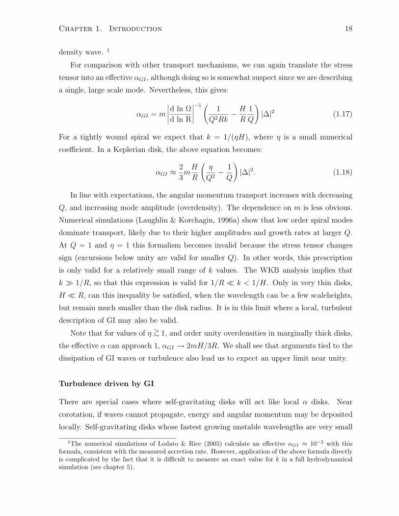
Chapter 1. Introduction 18
density wave. 1
For comparison with other transport mechanisms, we can again translate the stress
tensor into an e!ective (GI , although doing so is somewhat suspect since we are describing
a single, large scale mode. Nevertheless, this gives:
(GI = m
)))))d ln %
d ln R
)))))
!1 %1
Q2Rk& H
R
1
Q
&
|'|2 (1.17)
For a tightly wound spiral we expect that k = 1/(/H), where / is a small numerical
coe#cient. In a Keplerian disk, the above equation becomes:
(GI (2
3m
H
R
%/
Q2& 1
Q
&
|'|2. (1.18)
In line with expectations, the angular momentum transport increases with decreasing
Q, and increasing mode amplitude (overdensity). The dependence on m is less obvious.
Numerical simulations (Laughlin & Korchagin, 1996a) show that low order spiral modes
dominate transport, likely due to their higher amplitudes and growth rates at larger Q.
At Q = 1 and / = 1 this formalism becomes invalid because the stress tensor changes
sign (excursions below unity are valid for smaller Q). In other words, this prescription
is only valid for a relatively small range of k values. The WKB analysis implies that
k + 1/R, so that this expression is valid for 1/R , k < 1/H. Only in very thin disks,
H , R, can this inequality be satisfied, when the wavelength can be a few scaleheights,
but remain much smaller than the disk radius. It is in this limit where a local, turbulent
description of GI may also be valid.
Note that for values of / >$ 1, and order unity overdensities in marginally thick disks,
the e!ective ( can approach 1, (GI * 2mH/3R. We shall see that arguments tied to the
dissipation of GI waves or turbulence also lead us to expect an upper limit near unity.
Turbulence driven by GI
There are special cases where self-gravitating disks will act like local ( disks. Near
corotation, if waves cannot propagate, energy and angular momentum may be deposited
locally. Self-gravitating disks whose fastest growing unstable wavelengths are very small
1The numerical simulations of Lodato & Rice (2005) calculate an e!ective !GI ( 10!2 with thisformula, consistent with the measured accretion rate. However, application of the above formula directlyis complicated by the fact that it is di"cult to measure an exact value for k in a full hydrodynamicalsimulation (see chapter 5).

Chapter 1. Introduction 19
compared to the radial extent of the disk (large / - 1/(kH)) are also amenable to a local
( treatment.
The importance of the latter case, where gravitational instability successfully gener-
ates small scale, (-like turbulence was first demonstrated by the numerical simulations
of Gammie (2001), who showed that a gaseous self-gravitating disk could enter into a
self-regulated state of turbulence if two conditions were satisfied.
A razor thin, Q $ 1 disk satisfies the large wavenumber (small wavelength) require-
ment. In order for the disk to enter a self-regulated state of local “gravito-turbulence,”
local dissipation of the turbulence must be balanced by heating. This second, so-called
cooling constraint is:
tcool = U
)))))dU
dt
)))))
!1
$ %!1 % $c2s
!T 4e"
. (1.19)
where ! is the Stefan-Boltzman constant, and U is the internal energy of the disk. If
the heating due to turbulent dissipation is too weak, then the disk collapses on scales
comparable to the scaleheight as discussed above. If the heating is so strong that it
raises the disk temperature, and thus cs, the disk will restabilize at a value of Q > 1.
However, if heating by dissipation just balances cooling, the disk can self-regulate to
remain unstable and turbulent, but not fragment into bound objects. In this case, the
e!ective transport due to disk self-gravity can be translated directly into an ( as:
( =1
0(0 & 1)
4
9%tcool(1.20)
where 0 is the adiabatic index of the gas. Note that this prescription allows us to
determine a maximum ( beyond which fragmentation occurs, although its value may
depend on 0 and the disks energy source (Rice et al., 2005). For a discussion of maximum
accretion rates due to disk self gravity in the AGN context, see Shlosman & Begelman
(1987).
In chapters 4 and 6 we discuss this process in more detail, review recent literature
in the area, and show how this constraint might be altered in di!erent environments.
In particular we shall see that for realistic disk densities, temperatures and opacities,
heating by dissipation can not always just balance cooling, implying that not all disk
locations can become gravitoturbulent.

Chapter 1. Introduction 20
1.3.3 Transport by an External Perturber
The foundational work on angular momentum transport by external perturbers was con-
ducted by Goldreich & Tremaine (1979). Waves due to external perturbers are launched
at the outer Lindblad resonance. If they remain linear, and propogate inward, then they
carry with them angular momentum. As they propagate inward, the ratio of the wave
pattern speed to the disk orbital frequency decreases. Once waves cross the corotation
radius they are then rotating more slowly than the background disk and hence carry
negative angular momentum. If the waves eventually dissipate, giving up angular mo-
mentum to the local region, the disk loses angular momentum, and the perturber gains
it (Goldreich & Tremaine, 1979). Though it is beyond the scope of this discussion, this
theory laid the ground work for the theory of planet migration.
For transport to occur, the waves must propagate as weak shocks so that dissipation
occurs gradually, rather than on the lengthscale on which it is launched (Savonije et al.,
1994). If one requires that the wave amplitudes are marginally non-linear, the e!ective
( scales inversely with the local Mach number of the Keplerian flow (Papaloizou & Lin,
1995). Thus this dissipation mechanism should be most e!ective in thick disks, where
the flow is least supersonic.
For the remainder of the thesis we will mostly ignore the role of external perturbers
because we are primarily concerned with the disk processes that lead to the formation
of the companion, rather than the evolution thereafter. While perturbations due to a
stellar encounter, for example, can drive accretion, they ultimately stabilize marginally
gravitationally unstable disks, rather than drive fragmentation (Forgan & Rice, 2010).
In chapters 5 and 6 we discuss some of the e!ects of companions on disks. In the
former we discuss how these e!ects may control the final orbital distribution of disk born
binaries, and in the latter we examine how interaction between the disk and perturber
can control the growth of objects born in disks.
1.4 Numerical Techniques
A significant portion of this thesis is based upon numerical experiments, and so I briefly
review the methods employed here, and the advantages of the chosen technique. We use
the code ORION to conduct our numerical experiments (Truelove et al., 1998; Klein,
1999; Fisher, 2002). ORION is a parallel, adaptive mesh refinement (AMR), multi-fluid,

Chapter 1. Introduction 21
radiation-hydrodynamics code incorporating self-gravity and Lagrangian sink particles
(Krumholz et al., 2004). Radiation transport and multi-fluids are not used in this study.
1.4.1 Hydrodynamic Solver
The gravito-hydrodynamic equations are solved using a conservative, Godunov scheme,
which is second order accurate in both space and time. Godunov schemes solve the
Riemann problem to calculate the flux of conserved quantities across grid cells. The
Riemann problem is a more general version of the shock-tube problem in which the
form of a wave traveling across the boundary can be composed of a right or left moving
rarefaction wave or shock, joined by a contact discontinuity. The exact Riemann problem
is solved by finding the root of an algebraic pressure equation derived from both the
Rankine-Hugoniot jump shock conditions, and standard ideal gas equations. A numerical
algorithm must be employed to iteratively find the root. Once the pressure equation is
solved, the ideal gas equations can be used to find the remaining primitive variables (', u)
and thus the conserved quantities (', 'u,E).
In practice, solving the exact Riemann problem at every interface at every timestep
is extremely time consuming and unnecessary to adequately compute the fluxes. Conse-
quently, ORION uses an approximate solution to the Riemann problem, which provides
su#cient accuracy with large improvements in e#ciency (Toro, 1997). ORION is opera-
tor split, meaning that at each time step, each coordinate direction is solved for cyclically.
For a more detailed description of the specific Godunov method used in ORION, includ-
ing a description of the characteristic tracing technique and use of artificial fluxes, see
Truelove et al. (1998).
1.4.2 Adaptive Mesh Refinement
Adaptive Mesh Refinement (AMR) is a technique to dynamically and hierarchically al-
locate new, higher resolution grids within a simulation in regions that are becoming
under resolved as defined by some user criteria. For our study of rapidly accreting disks,
AMR allows us to achieve two goals simultaneously. First, we can set up simple initial
conditions which place the computational boundary far from the disk by adding computa-
tionally inexpensive, coarsely refined zones to the outer regions. Secondly, we can resolve
both the background flow and disk simultaneously, and let the disk expand in time as it
accretes higher angular momentum material. This means that a given run becomes more

Chapter 1. Introduction 22
computationally expensive in time. The corollary of course is that the requirements at
the beginning of a run are relatively modest when there is little to resolve. In addition
to adaptive gridding, ORION also uses adaptive time steps, so that low resolution grids
are evolved based on the local courant condition, not on that calculated for the highest
level. As a result, following the evolution of gas on large scales at low resolution is very
computationally e#cient.
1.4.3 Gravity Solver
Because ORION uses AMR, it is e#cient to take advantage of the hierarchical domain
decomposition done by the hydrodynamic solver and use a multigrid method to solve
the Poisson equation for the current density distribution. The multigrid method uses
a relaxation technique to solve the system of sparse linear equations that result from
discretizing the Poisson equation on each level. The advantage of this technique is that
the solutions found on coarse grids can be used to correct for low-frequency errors, while
the higher resolution ones extract high-frequency errors. The result is faster convergence,
because more iterations are done on coarse rather than fine grids. The gravitational
potential is then used as a source term in the gravito-hydrodynamic equations.
1.4.4 Sink Particles
Each year, Moore’s Law suggests that we can consider previously intractable computa-
tional problems. For example, over the course of this thesis, the local available super
computers have increased from hundreds of processors to close to 10,000. Nevertheless
the dynamic range we can explore remains limited even in adaptive codes such as ORION.
The most stringent limitation on dynamic range in this case comes not from the
grid resolution, but from the time resolution. The hydrodynamic timestep is limited
by the Courant condition, which requires that the timestep be smaller than the signal
crossing time of a grid cell. As densities increase within a given cell, the signal crossing
time decreases, requiring very fine timestepping. In particular, in the case of Keple-
rian flows studied here, as the physical resolution increases, the distance to the central
masses decrease, and so the rotational velocities we must resolve increase. Since, as we
discuss in chapter 5, we resolve entire disks at the same resolution, small time steps be-
come extremely prohibitive. Moreover, because processor speeds of individual cores are
increasing modestly compared to the number of cores over which a problem can be paral-

Chapter 1. Introduction 23
lelized, limitations on timesteps are much more prohibitive as they cannot be computed
simultaneously.
Although not as severe a limitation computationally, to prevent unphysical fragmen-
tation, the Jeans length, which decreases with increasing density, must be resolved by a
su#cient number of grid cells (Truelove et al., 1997). This can also make calculations of
a high density central star or fragment in a disk computationally prohibitive.
In order to perform a numerical parameter study at high resolution, to follow many
disk orbits, and to complete the computations on a thesis timescale, we have employed
sink particles rather than resolve very high density regions. Sink particles form when the
gas becomes unresolved based on the Truelove criterion, and then continue to accrete
nearby gas, and interact with it and any other sink particles gravitationally. See both
chapter 5 and Krumholz et al. (2004) for a detailed description of the sink particle
algorithm. Generally, the accretion rate onto the sink uses an approximate Bondi-Hoyle
formula, where values for the density and sound speed at infinity are set di!erently
depending on the relative ratio of the grid size to the Bondi radius. There is also an
additional check on the angular momentum of nearby gas, so that unbound gas does not
accrete.
The use of sink particles means that one loses resolution within the accretion scale of
a particle, but it makes it feasible to study fragmentation and binary formation in a full
three-dimensional disk calculation. Perhaps one of the most important features of this
method for our purposes is the ability to have a moving central stellar potential, rather
than one fixed to the grid. As discussed in chapter 5, this allows us to study transport
driven by both even and odd m spiral modes which perturb the star from the center
of mass when the disk mass becomes large. It also enables us to study the influence of
on-going accretion and eccentricity in binary orbits.
1.4.5 Three Dimensional Disks and Cartesian Grids
Keplerian accretion disks are approximately two dimensional structures. For the purposes
of computational e#ciency, many have chosen to follow the approach laid out in §1.3
of integrating over the vertical direction and simulating the disk in two dimensions.
This approach is extremely fruitful for studying many aspects of disk behavior including
angular momentum transport by gravitational instability. However, for the specific case
which we study here – disks fed at their outer edges – resolving the vertical structure

Chapter 1. Introduction 24
is more important. Massive disks in this regime are not geometrically thin and develop
moderate turbulent motions in the vertical direction. Although not borne out by our
studies thus far, we initially hypothesized that this stirring could support disks and
provide transport at values significantly exceeding ( $ 1. Our fully three dimensional
setup also gave us insight into interesting shock structures forming where the inflow
impacted outward moving spiral arms. These and other features may be examined further
in future work.
Although disk problems are inherently ill-suited to cartesian codes due to numerical
di!usion e!ects, ORION provided the best combination of computational features for
our chosen problem. As we describe above, a main requirement for this work was a
moving central potential. Due to the singularity at the center of cylindrical domains,
implementing a moving potential in that geometry can be challenging. Moreover, due
to the extensive use of this code implementation for disk-like problems, the numerical
di!usion has been well characterized.

Chapter 2
Observational Connections:
Multiplicity and Star Formation
2.1 Introduction
The study of binarity dates back at least 250 years to Mitchell (1767), who pointed
out the abundance of double stars. Many tout the 21st century as the era of precision
cosmology, but we are also entering the era of precision in more classic “astronomy” –
understanding the ordering of the stars. Great technological advances including the use
of coronography (Hinkley et al., 2007) and adaptive optics (Lafreniere et al., 2009) have
brought stellar companions into better focus. Despite the longevity of these studies, and
the recent advances, we still lack a comprehensive model for the formation of binaries
and higher order multiples.
Theories of star formation have been influenced by our heliocentric bias. Until re-
cently, our models have reflected that we live next to a relatively low mass star (ap-
parently) without a stellar or substellar companion. The seminal work of Duquennoy
& Mayor (1991) on the multiplicity of sun-like stars showed that our sun is somewhat
unusual in being alone. Although the statistics are incomplete for stars of other masses,
it now also seems clear that there is a strong correlation between stellar mass and mul-
tiplicity (Lada, 2006; Mason et al., 2009). The M stars, the most common stars in the
galaxy, are usually in single systems. As primary mass increases to just a few solar
masses, binaries become ubiquitous, even as the stars themselves become quite rare. The
data are consistent with all O and B stars having at least one stellar companion at birth.
The statistics on higher order multiplicity are still incomplete. It remains di#cult to
25

Chapter 2. Observational Connections 26
detect relatively close, small mass ratio pairs, particularly for massive primaries. Up-
coming searches with next generation infrared telescopes such as JWST may improve
these statistics.
Armed with this new data, it is time to reconsider our models of single and multi-
ple star formation. To be sure, conclusions drawn from the current data require many
caveats. We do not have a complete picture of companions at all separations and mass
ratios. Moreover, given the diverse nature of these systems, it is unlikely that one mech-
anism can explain them all. For example, it seems unlikely that equal mass, massive
twins (Krumholz & Thompson, 2007), and brown dwarf binaries separated by thousands
of AU (Burgasser et al., 2009) could form by the same mechanism.
2.2 Standard Theories of Binary and Multiple Star
Formation
There are several prominent theories of binary and multiple star formation in the litera-
ture. They can be divided roughly into three categories based on the timescale at which
the binary forms relative to the star formation process. I review theories for binary for-
mation (1) at the onset of star formation, (2) during disk-mediated accretion, and (3)
during the early phase of star-cluster evolution. In this review I neglect theories of binary
formation that occur after the bulk of the star formation process has occurred. There is
strong observational evidence that formation happens at early times as seen through the
higher binarity fraction in pre-main sequence stars as compared to main sequence stars
(Mathieu, 1994). I begin with a brief description of each theory, and proceed to compare
them with the best observational evidence to date.
2.2.1 Core Fragmentation Theories
The most common mechanisms in the literature fall into the first category, and are
described alternately as prompt or early fragmentation, or more specifically as core or
turbulent fragmentation (Hoyle, 1953; Tsuribe & Inutsuka, 1999a; Boss et al., 2000;
Padoan & Nordlund, 2002; Fisher, 2002). The earliest fragmentation scenario is that
of Hoyle (1953) who argued for opacity-limited hierarchical fragmentation, whereby an
unstable cloud keeps fragmenting at the local Jeans mass, which decreases as the cloud
collapses to higher densities, until the smallest fragments become optically thick and

Chapter 2. Observational Connections 27
can no longer cool e#ciently. There are numerous reasons why this mechanism is both
unphysical and inconsistent with the observed stellar mass function (for a thorough review
see Fisher 2002). Nevertheless, this mechanism gave birth to more modern theories of
core fragmentation.
In the subsequent generation of “core” fragmentation scenarios, a collapsing, bound
gas clump was thought to fragment into two or more objects depending on the ratio of
thermal to gravitational energy, ( = 5c2sR/GM , and the ratio of rotational to gravi-
tational energy, & = %2R3/3GM . Inherent in this parameterization is the assumption
that any dynamically important magnetic fields have already di!used out (or can be
included simply as an extra e!ective pressure in the calculation of (). When the product
(& < 0.12, cores were initially thought unstable (Inutsuka & Miyama, 1992), although
this model has the somewhat counterintuitive result that slowly rotating (small &) virial-
ized cores remain prone to fragmentation. More recent work has shown this criterion to
be incomplete, requiring also that ( <$ 0.5 (Tsuribe & Inutsuka, 1999b). Yet this model
neglects many thermal e!ects as the gas collapses to higher densities, and would seem to
over produce short period binaries.
The source of angular momentum setting & in the model above was thought classi-
cally to be galactic shear (Bodenheimer, 1995), but more recent investigations show that
the ubiquitous turbulence in the interstellar medium could also be responsible for the
observed line-width size relations interpreted as evidence of core rotation (Fisher, 2004;
Goodman et al., 1993). This has led to yet another class of models, appropriately termed
turbulent fragmentation. The former scenario relied on a linear instability, whereas the
turbulence scenario suggests that non-linear perturbations expected in a turbulent cloud
can cause a sub-region within a core to become overdense and collapse more rapidly than
the free-fall timescale of the background core, thereby leading to the production of a
secondary clump within the bound core. Alternatively, turbulent motions can lead to
the formation of filamentary structures which then fragment into multiple objects. These
stars are presumed to accrete from their natal core mostly independently.
Note that there is another class of star formation models dubbed turbulent fragmenta-
tion or “gravoturbulent fragmentation” which refers to the fragmentation of a molecular
cloud on larger scales into many bound objects which form their own stellar systems
(Ballesteros-Paredes et al., 2007). The turbulence sets the mass-scale of the cores, and
their turbulent structures, but for the purposes of multiple formation we are concerned
with the subsequent fragmentation of the turbulent clump, not the process that generated

Chapter 2. Observational Connections 28
it.
2.2.2 Disk Driven Formation
Models for binary and multiple formation at a slightly later evolutionary state involve
protostellar disks. The two classic disk-driven models are disk fragmentation (Laughlin
& Bodenheimer, 1994; Bonnell & Bate, 1994a; Adams et al., 1989; Artymowicz & Lubow,
1996), and disk capture (Clarke & Pringle, 1991; Moeckel & Bally, 2007). The former,
to which much of this thesis is dedicated, suggests that some stars will form su#ciently
massive protostellar disks that become susceptible to gravitational instabilities. If disks
become su#ciently unstable, and the gas can cool e#ciently, the disks can fragment
to produce one or more coplanar companions that accrete from the parent disk, and
depending on the formation epoch, the primary’s natal cloud.
Disk fragmentation has received renewed attention from numericists in recent years.
Prior work on this topic has been severely limited by two assumptions. The first is that
disks can be modelled in isolation. Disks modelled in the absence of ongoing accretion
are much less likely to become unstable. As we show in the course of this thesis, ongoing
accretion at the outer edge of the disk is often necessary to drive instability.
The second related assumption was that disks are always low in mass relative to
the central star. Certainly observed T-Tauri disks tend to be lower in mass, but as
observations improve we are beginning to observe more massive disks at early epochs of
formation (Andrews & Williams, 2007). Together these two notions led most previous
authors to conclude that disk fragmentation might occur rarely, and could only produce
very unequal mass ratio objects, which was inconsistent with binary statistics.
However, if disks are more massive and undergo continued accretion, simulations
suggest that fragmentation may be more common, and that secondaries born in the disk
can accrete quickly to catch up to the primary in mass (Bonnell & Bate, 1994b; Krumholz
et al., 2009; Kratter et al., 2010). Together with observations of more massive disks, this
suggests that the disk scenario can in fact produce a wide range of mass ratios, although
we find that this mechanism is most likely relevant for systems with primaries more
massive than our sun.
Following fragmentation, subsequent interactions between circumstellar and circumbi-
nary disks may further alter their orbits: gravitational torques can expel the circumbi-
nary disk carrying away a large fraction of the orbital angular momentum (Chang et al.,

Chapter 2. Observational Connections 29
2009). By contrast, tidal interactions between each of the two circumstellar disks allow
for transfer of angular momentum from the disks to the orbit, expanding it as in the case
of the Earth-Moon system where the rotation of the disk / Earth is faster than that of
the orbit of the binary star / Moon. The latter interaction becomes important only when
the protostellar disk fills the e!ective Roche radius of the star-disk system, and so may
not be the dominant driver of orbital evolution.
In the capture scenario, a massive disk increases the gravitational cross-section for
capturing a nearby star into a bound orbit. Although initial investigations found this
process to be highly ine#cient around low mass stars at reasonable stellar densities
(Clarke & Pringle, 1991), more recent work suggests that the process might be better
suited for massive stars with correspondingly more massive disks (Moeckel & Bally, 2007).
2.2.3 Multiple Formation in a dynamically evolving cluster
A final, more global mechanism for multiple formation is that put forth in a series of
papers including Bate (2000), Bate et al. (2003), and Bonnell et al. (2004). These mod-
elers suggest that star clusters form through a dynamic process of competitive accretion.
In this scenario, a turbulent molecular cloud forms many roughly Jeans mass clumps
that interact with one another and compete for mass from the background cloud. In
this environment there are multiple mechanisms for binary formation, including the disk
methods mentioned above, as well as dynamical interactions between three or more bod-
ies which can eject a low-mass object and tighten the orbits of the remaining bound pair.
In addition, dynamical friction between the protostars and background gas is thought to
tighten wider binaries. What distinguishes this scenario from those listed above is that a
stellar system does not accrete from a fixed, marginally bound core, but rather migrates
around in a cloud collecting previously unbound material.
A related model put forth by Goodwin & Kroupa (2005) relies on a combination
of the core fragmentation and dynamical evolution hypothesis to reproduce the high
multiplicity fraction of young stars in clusters, compared to their field star counterparts.
Although they do not specify the precise mechanism for fragmentation, these authors
imagine that most cores either break up into 2 or 3+ individual stars. Through dynamical
interaction, the higher order multiples evolve into single star systems, tight binaries,
and stable hierarchical systems. They posit that di!erent clusters environments (which
have di!erent rates of close stellar encounters) will naturally evolve to show di!erent

Chapter 2. Observational Connections 30
multiplicity fractions.
2.3 Observational Tests of Theoretical Models
Advances in numerical techniques mean that each of the processes described above has
been simulated at high resolution. Though numerical artifacts remain, many of the mech-
anisms cannot be ruled out on basic physical grounds. Instead they must be evaluated
based on their ability to reproduce the observables of the star formation process. This
is di#cult to measure precisely, as it would require that we know the conditions in a
given cloud and core over its entire formation timescale, which is clearly unobservable.
Although much progress has been made characterizing the di!erent phases of core for-
mation as described in chapter 1, one must also compare the predicted properties of the
stellar mass distribution in terms of mass ratios, periods, eccentricity, etc. Selection ef-
fects and the complexities of the theories make this challenging and uncertain, but it is a
goal worth pursuing. We must, however, exercise some caution when assessing theories of
binary formation which reproduce observed trends, but fail to address the fundamental
physics underlying formation. While the e!ort to create models which reproduce obser-
vations is important, we should not neglect detailed modeling of molecular clouds and
prestellar cores from which binaries form.
2.3.1 Empirical Models for Turbulent Fragmentation
Semi-empirical models such as Fisher (2004) have had some degree of success producing
observed period and mass ratio distributions of low mass stars from the turbulent frag-
mentation mechanism. This work assumes that the components of binaries are drawn
randomly from the initial mass function (IMF), and that there exists a constant e#ciency
factor with which mass and angular momentum are transferred from the core to the bi-
nary. They also draw eccentricities randomly from a thermal distribution, consistent
with observations, in order to specify the orbit for a given binary angular momentum. A
major limitation of this work is that the physical process which governs the distribution
of mass and angular momentum between binary components is ad hoc, and tuned to
reproduce the observations. While numerical work has shown that a multiple system
can form out of a turbulent core, it remains to be shown in detail that the e#ciency of
angular momentum and mass removal scales as this model suggests. Moreover, while the

Chapter 2. Observational Connections 31
final distribution of binary systems is consistent with the observation distribution of low
mass stars, it is not consistent with the orbital parameters and mass ratios for substel-
lar companions and more massive stars. Recent AO surveys by Metchev & Hillenbrand
(2009) show that the distribution of substellar companions to solar-type stars is inconsis-
tent with being randomly drawn from the IMF. There is also a dearth of substellar mass
companions at large distances. On the opposite end of the mass spectrum there may also
be inconsistencies. First, there is no clear explanation for the increase in binarity with
core mass in this model. Secondly, recent numerical work (Krumholz et al., 2007b) has
shown that radiation from the first star can suppress turbulent fragmentation in massive
cores because more massive protostars are luminous even at early times.
2.3.2 Competitive Accretion and the IMF
Similarly, the competitive accretion picture has had moderate success explaining portions
of the observed initial mass function (Moeckel & Bate, 2010) and binary statistics. How-
ever, these models tend to overproduce the binaries containing the lowest mass stars and
brown dwarfs, and have higher star formation e#ciencies than observed (Price & Bate,
2009). Another major criticism is that the relative velocities between accreting cores and
background gas are so high that the accretion rate onto the cores should be far too low to
produce more massive stars (Krumholz et al., 2006). In addition, the intercore velocities
appear to be much higher in the simulations than observed between actual star forming
cores, calling into question whether or not there can be significant core-core interaction
on the timescale of star formation (Kirk et al., 2009; Evans et al., 2009).
The Goodwin & Kroupa (2005) picture does reproduce the observations for stars<$ 1M", but like the model of Fisher (2004) it has been tuned to do so. The mechanism
which breaks some cores into two versus three stars, and the division of mass and angular
momentum between them is not specified in detail.
The dynamical interactions observed here may be key to forming wide, very low
mass binaries. Some have suggested that these few body interactions which occur as
the initially bound cluster begins to spread could produce weakly bound brown dwarfs
(Kouwenhoven et al., 2010).

Chapter 2. Observational Connections 32
2.3.3 Disk fragmentation: a possible solution to the luminosity
and angular momentum problems
As we show in chapter 5, the disk scenario can produce a range of stellar separations and
mass ratios, depending on primary mass, and the epoch of disk instability. Although no
statistical study of this process has been completed, investigations are ongoing (O!ner
& Kratter, 2010 in prep). Nevertheless, the disk fragmentation scenario may be consis-
tent with two observational puzzles in star formation: the so-called luminosity problem
(Kenyon et al., 1990) and the angular momentum problem (see Bodenheimer 1995 and
references therein).
The luminosity problem refers to the discrepancy between the observed and predicted
bolometric luminosity of young protostars based on their accretion luminosities. Given
a star formation timescale and stellar mass, we can predict the time-averaged mass ac-
cretion rate, and thus the corresponding luminosity. While uncertainties in the opacities
and geometry of high extinction cores can complicate the interpretations, recent data
from the Spitzer c2d survey confirms that most young sources are underluminous com-
pared to the expected luminosity from the time-averaged rate (Evans et al., 2009). These
authors suggest that variable, high accretion rates, particularly in the Class 0/I phase,
are all but required by the data. Because so few cores are observed to have luminosities
consistent with the time averaged rate (a few 10!6M"/yr) accretion must occur in short
bursts ($ 104 years) well above this rate.
For more massive protostars, these high, variable accretion rates at early times are
consistent with infall at rates such that " - MG/c3s + 1, which we shall show are
susceptible to fragmentation. Although we study steady accretion here, highly variable
accretion from turbulent cores could further promote fragmentation if the disk is fed
asymmetrically, which may also be consistent with observations (see e.g. Tobin et al.
2010).
The angular momentum problem refers to the fact that we do not understand how
four orders of magnitude of angular momentum are repartitioned between the largest
scales in Giant Molecular Clouds (GMCs), where the specific angular momentum is set
by the di!erential rotation in the galaxy (Bodenheimer, 1995) and the scales of binary
orbits. By the time dense cores have formed, line-width size observations reveal that the
typical specific angular momentum has dropped by two orders of magnitude (Goodman
et al., 1993). When we look at binary stars, whose formation is intimately tied to the

Chapter 2. Observational Connections 33
core angular momentum, the average specific angular momentum can drop another two
orders of magnitude.
Magnetic fields may play an important role in removing angular momentum on the
largest scales (Li et al., 2004), although hydrodynamic turbulence can be significant
as well (Jappsen & Klessen, 2004). Disk fragmentation may be important on smaller
scales: because disk size is regulated by the gas reservoir’s angular momentum, if the
disk fragments to form a binary or multiple before all of the infalling gas and angular
momentum has accreted onto the star-disk system, binaries can form with less orbital
angular momentum than that contained in the core. Subsequent few-body interactions
in disk-born higher order multiple can also redistribute angular momentum by expelling
the lowest mass companions.
Several other trends seem roughly consistent with the disk scenario. Both disk frag-
mentation and binary frequency increase with primary mass. At lower masses where disks
are stabilized by stellar irradiation (Matzner & Levin, 2005), the turbulent cores out of
which they form may be more susceptible to early fragmentation (O!ner & Kratter, 2010
in prep).
The trend towards equal mass components at very high masses might be related to the
fact that massive disks become unstable early on in their accretion histories (Pinsonneault
& Stanek, 2006). There are also hints in the high mass multiplicity statistics that mass
ratio scales inversely with separation (Mason et al., 2009). Although migration can alter
the orbits, disk fragmentation suggests a possible correlation between secondary mass
and separation: fragmentation typically occurs towards the outer edge of the disk which
is larger at late times at which point there is also less mass available for the secondary
to accrete.
A final piece of evidence favorable for the disk scenario is the observation that binaries
separated by less than rougly 40 AU are more likely to have the stellar spins aligned with
the binary orbit (Hale, 1994). Although this study does not account for higher order
multiples, and has significant uncertainties in the measurements (e.g. sin i), this is
suggestive that perhaps some objects were born in disks. Of course objects born from
clouds with the same net rotation might also tend to be aligned, although stars born
from turbulent cores might sample the turbulent spectrum from di!erent parts of the
core with di!erent net angular momentum vectors.

Chapter 2. Observational Connections 34
2.4 Conclusions
Despite their ubiquity, we still lack a coherent theory of binary and multiple star forma-
tion which can explain the enormous range of observed systems. We have demonstrated
that disk fragmentation requires more careful consideration as one of several viable mech-
anisms, especially for stars more massive than our sun. Several on-going projects attempt
to quantify this statement. We must investigate whether or not the fraction of cores that
produce su#ciently high disk masses for fragmentation are consistent with binary frac-
tions as a function of primary mass. We must also construct a model for the orbital
evolution of binaries formed in disks. Current theories are limited to either extreme mass
ratios (e.g. planets), or simplified cases (circular orbits).

Chapter 3
Disks in the Formation of Massive
Stars
A version of this chapter has been published in the Monthly Notices of the Royal Astro-
nomical Society as “Fragmentation of massive protostellar discs”, Kratter, K. M., and
Matzner, C. D., vol. 373, pp1563-1576, 2006. Reproduced by permission of MNRAS.
3.1 Introduction
We begin by examining the role of accretion disks in the formation of massive stars.
Advances in submillimeter telescopy have enabled the discovery of flattened structures, in
some cases clearly Keplerian disks, surrounding massive ( >$ 10M") protostars (Cesaroni,
2005; Chini et al., 2004; Patel et al., 2005; Beuther et al., 2006). The logical inference
– that high mass star formation (HMSF) proceeds through disk accretion – raises a
question: can such disks process rapid mass accretion, or do they fragment to produce
secondary stars? We seek to answer this question by estimating the criterion for disk
fragmentation in the vicinity of a massive star.
If massive-star disks typically do not fragment, then disk accretion poses little barrier
to massive star formation. Conversely if disk fragmentation occurs, then accretion onto
the central star may be (partially) choked o!, as suggested by Tan & Blackman (2005)
in the context of low-luminosity active galactic nuclei. Moreover each massive star that
forms from a fragmenting disk may be surrounded by smaller stars that began as disk
fragments. It is therefore important to evaluate models for HMSF in light of the disk
fragmentation criterion.
35

Chapter 3. Disks in the Formation of Massive Stars 36
The current work uses and extends the results of Matzner & Levin (2005, hereafter
ML05), who showed that protostellar disks around low mass stars are strongly stabilized
against fragmentation by a combination of viscous heating and irradiation by the central
protostar. Massive star formation is fundamentally di!erent, however, in three important
ways. The rapid rise of luminosity with mass implies that stellar irradiation is far more
intense; this tends to stabilize disks against fragmentation. However, massive stars must
accrete quickly to form at all (e.g., Wolfire & Cassinelli, 1987), and rapid accretion favors
fragmentation. These e!ects compete to set the critical radius outside of which disks
fragment. Whether fragmentation actually occurs depends on the initial disk radius,
which itself depends on the physical state of the gas prior to accretion. We discuss
disk fragmentation in §3.2, considering the stabilizing e!ect of viscous heating (§3.2.2)
before incorporating irradiation by the central star (§3.2.3). This combination allows
us to identify (§3.2.4) the disk radius at which fragmentation sets in. The McKee &
Tan (2003) core collapse model is examined in more detail in §3.3: we compute angular
momentum scales in §4.3.4 using formulae derived in the Appendix. In §3.4 we calculate
expected fragmentation radii for a range of masses in the core collapse model.
Turning to the consequences of fragmentation, we examine in §3.5 the likely properties
of stars born within fragments and the possibility that fragmentation limits accretion.
In §3.5.2 we compare our results with observed regions of HMSF.
3.2 Disk Fragmentation
3.2.1 Criterion for Fragmentation
We shall concentrate on fragmentation due to local gravitational instabilities, which set
in when Toomre’s parameter
Q =cad%
.G$(3.1)
descends toward unity. Here $ is the disk’s surface density, % its orbital frequency, and
cad is its adiabatic sound speed. (We shall frequently refer to the isothermal sound speed
cs = 0!1/2cad where 0 is the ratio of specific heats.)
Observational inferences of massive circumstellar tori (Cesaroni, 2005) indicate that
they may be subject to global instabilities as well. We discuss this possibility briefly in
§3.4.4; however the local instabilities tend to occur first, and their relation to fragmen-
tation is better understood.

Chapter 3. Disks in the Formation of Massive Stars 37
Several authors have identified the fragmentation boundary in terms of a cooling time.
Following Gammie (2001) and ML05, we convert this criterion to a critical mass accretion
rate at a given midplane temperature. The cooling time 1c is the ratio of the internal
energy per area, U = c2ad$/[0(0 & 1)], to the dissipation rate per unit area – which, in
steady accretion, is
2Fv =3M%2
4.(3.2)
where Fv is the flux through each disk face. Eliminating $, the maximum accretion rate
is
Mmax =401/2
3(0 & 1)
c3s
Q%1cG. (3.3)
For later convenience we write this in terms of the isothermal sound speed cs = 0!1/2cad.
Extrapolating from Gammie (2001)’s two-dimensional simulations for a sti! equation of
state, ML05 estimate Mmax = 0.89c3s/G for the case of a three-dimensional, 0 = 5/3
disk. Using smoothed-particle hydrodynamics, Rice et al. (2005) have simulated just
such a disk, finding %1c to lie between 6 and 7 when it fragments. Assuming also Q = 1,
this implies Mmax = (0.37 to 0.43)c3s/G. For a fixed M , the critical temperature is then
significantly (1.6 times) higher than ML05 estimated.
At face value this weakens the conclusion, reached by ML05, that fragmentation is
unattainable in low-mass protostellar disks. However, more recent simulations show that
disks remain stable at shorter 1c depending on how abruptly cooling is implemented
(E. Harper-Clark 2006, private communication). Due to uncertainties in the aforemen-
tioned cooling factor, and in light of the stringent resolution requirements for collapse
outlined by Nelson (2006), we consider the value of %1c obtained by Rice et al. (2005) to
be uncertain by up to a factor of two. We shall therefore be conservative, by adopting
the stricter ML05 criterion that fragmentation occurs when
cs < cs,crit = 1.04(GM"d)1/3. (3.4)
Since the mass accretion rate is comparable to %ce"(core)3/G in the core collapse scenario,
where ce"(core)2 is the ratio of pressure to density in the core, equation (3.4) implies,
qualitatively, that a disk fragments if its sound speeds falls below the e!ective sound
speed of its parent core (see equation [3.23] below). This point was made for thermally
supported cores by ML05, and equation (3.4) simply extends the rule to turbulent cores.
Equation (3.4) is conservative in the sense that fragmentation may also occur at
somewhat higher values of cs. It is even more conservative given that 0 declines from 5/3

Chapter 3. Disks in the Formation of Massive Stars 38
at the higher temperatures relevant to massive star formation. We shall make several
other conservative estimates in order to show that disk instability is all but inevitable
during massive star formation.
When assessing disk stability in a given scenario, we first calculate the midplane
temperature profile cs(r) of the disk given its central mass M", central luminosity L",
and accretion rate M"d. For this we adopt the Shakura & Sunyaev ( parametrization of
viscosity, in which the steady mass accretion rate is
Mvisc =3.($c2
s
%. (3.5)
For the choice of critical temperature made in equation (3.4) this corresponds to ( =
0.30Q at the onset of fragmentation. We keep ( fixed at 0.30 throughout our analysis, as
this correctly reproduces the fragmentation boundary, although this is an overestimate
for stable disks.
Having identified the fragmentation radius as the location where the disk sound speed
falls to the critical value in equation (3.4), we then compare this to the characteristic
disk radius
Rd =j2
GM"(3.6)
for accreting gas with specific angular momentum j.
We set the viscous accretion rate equal to the accretion rate from the envelope, and
let Q = 1. We then check whether the disk can remain in this steady state with two
models for heat generation. In §3.2.2 we ignore the luminosity from the protostar and
find a minimum value for Td(r) using only the viscous generation of heat. Next, in §3.2.3,
we include the flux from the protostar received at the disk surface, and again solve for
the midplane temperature as a function of radius.
3.2.2 Viscous Heating
In a thermal steady state, the flux of viscous energy radiated by each face of the disk
is given by equation (3.2). All of the disks considered in this chapter are optically thick
to their own thermal radiation; therefore, the flux can also be derived from radiation
transfer across an optical depth )$/2 from the disk midplane to its surface:
Fr =8
31R!T 4
d , (3.7)

Chapter 3. Disks in the Formation of Massive Stars 39
Subscript Meaning
cl .... Clump
c..... Core
2..... Star
d..... Disk
2d.... Star-disk system
f .... Final value
crit... Critical value for fragmentation
irr... Stellar irradiation
v..... Viscous flux
Table 3.1: Definitions of subscripts.
where 1R = )R$d/2 is the optical depth corresponding to the Rosseland mean opacity
)R(Td). The factor 8/3 in equation (3.7) is derived by assuming that the dissipation rate
per unit mass is a constant (Chick & Cassen, 1997). We obtain temperature dependent
opacities from Semenov et al. (2003). These opacities are very insensitive to density; we
adopt values for 10!12.5 g cm!3, an appropriate value for a disk with Q = 1 and a period
of a few centuries.
Neglecting irradiation of the disk surface, in a steady state Fv = Fr and Mvisc = M"d.
We solve for $ in equation (3.5), and then cs from equations (3.2) and (3.7) using µc2s =
kBT (for molecular weight µ), yielding
c10s =
3k4B)RM2
"d%3
128.2!µ4(. (3.8)
This is an implicit formula for cs, as )R depends on temperature. Equating cs to cs,crit
(equation 3.4) implies fragmentation when
% < 8.54
+
,!µ4(G10/3M4/3"d
k4B)R
-
.1/3
. (3.9)
In practice we calculate the run of cs(r) and )R(r) self-consistently in order to evaluate
equation (3.9).
Whereas ML05 found a unique value of %crit for optically thick accretion disks around
low-mass protostars, we shall show below that equation (3.9) gives a roughly constant
fragmentation radius of about 130 AU. The key di!erence is the higher accretion rate,
which implies much higher critical temperature (hundreds of K) in massive star formation

Chapter 3. Disks in the Formation of Massive Stars 40
compared to $ 16 K for the low mass case. As the opacity law does not obey )R(T ) % T 2
for these higher temperatures, the ML05 result does not hold for these more massive stars.
3.2.3 Stellar Irradiation
Stars of mass somewhat greater than 10M" undergo Kelvin-Helmholtz contraction rapidly
enough to settle onto the hydrogen burning main sequence while still accreting. As the
main sequence luminosity increases rapidly with M", the consequences of stellar lumi-
nosity become acute for massive stars. One such consequence is the heating of the disk
midplane due to reprocessed stellar radiation. In principle, this stabilizes disks to longer
periods (larger radii) than we found in equation (3.9) by considering only viscous heat-
ing. We parametrize irradiation through the reprocessing factor f defined as the ratio
between the incident flux Firr normal to the disk surface, and the spherical stellar flux at
that radius:
Firr =fL
4.R2d
. (3.10)
A calculation of f requires a model for the reprocessing of starlight onto the disk.
Infall geometry
ML05 model f in the context of an infall geometry similar to that used by Whitney
& Hartmann (1993) and Kenyon et al. (1993) for scattered-light images of protostars.
Starlight is absorbed at the inner edge of a rotating infall envelope (Terebey et al., 1984)
whose innermost streamlines have been removed by the ram pressure of a magnetically
collimated protostellar wind. This removal implies a suppression of the star-disk accretion
rate relative to the rate at which mass would otherwise accrete – from the surrounding
core, for instance, in a core-accretion model:
M"d = %Mc; (3.11)
where % = cos 30 if streamlines are removed from all angles within 30 of the axis. (We
assume the prestellar matter is isotropically distributed before it falls in.)
The balance of forces that determines % is modeled in detail by Matzner & McKee
(2000) for low-mass star formation, and we expect that their analysis holds into the
massive star regime. The location of the innermost streamline is a simple function of %:
it strikes the disk at a radius
(1& %2)Rd. (3.12)

Chapter 3. Disks in the Formation of Massive Stars 41
The calculation of f is particularly simple if the dust envelope is (1) optically thick
to stellar photons; (2) optically thin to dust thermal radiation; and (3) not hot enough
to sublimate. Under these conditions, ML05 find
f . 0.1%!0.35 (3.13)
for a reasonable range of %.
Envelope self-opacity and dust sublimation
It is important to examine the assumptions that led to equation (3.13), especially in the
context of very rapid accretion onto very massive stars.
In §4.3.4 we will estimate the typical infall column density $sph,f in a core collapse
scenario, and find it to be a few times lower than the core column $c, i.e., $sph,f . 0.3
g cm!2. Given that the Semenov et al. (2003) Planck opacity peaks between 3 and
16 cm2 g!1 for 45 < T < 930 K, we expect the disk midplane to be shielded by moderate
optical depths ($ 1 & 5) from the reprocessing surface. A solution to the radiation
di!usion problem is beyond the scope of this chapter . Instead we will apply equation
(3.13); this is conservative, in the sense that it overestimates the stabilizing e!ect of
irradiation.
A further potential complication arises for especially high accretion rates, those in
excess of 1.7) 10!3M" yr!1. The critical temperature of such a disk is quite hot, Tcrit >
1050 K according to equation (3.4). As we shall see in §3.4, the stabilizing e!ect of
irradiation is accentuated in these disks by a sharp drop in Rosseland opacity. If the
disk is to reach 1050 K, however, dust in the nearby infall envelope must approach the
silicate sublimation temperature of about 1500 K. This leads to the disappearance of
dust within the infall envelope inside a certain sublimation radius Rs. Monnier & Millan-
Gabet (2002) determine Rs . 35(L"/106L")1/2 AU by optical interferometry (and note
that this value requires the existence of large silicate grains). We expect that disks with
Rd > Rs are relatively una!ected by dust sublimation. We do not attempt to calculate
disk irradiation in cases where this is not true.
Incorporation into fragmentation calculation
Solving equation (3.10), we can find the equilibrium temperature of the outer reaches of
an optically thick disk for which irradiation dominates over viscous heating. While low-
mass protostellar disks can be stabilized in this regime (ML05), massive-star disks are
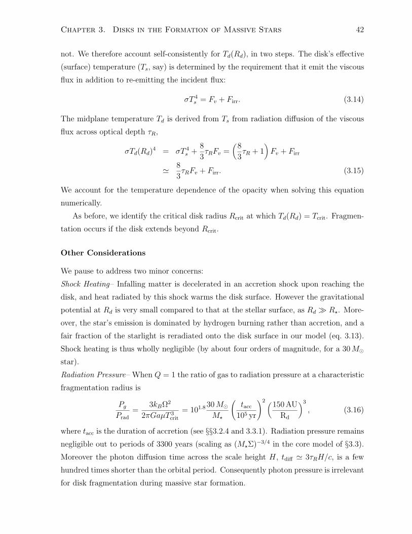
Chapter 3. Disks in the Formation of Massive Stars 42
not. We therefore account self-consistently for Td(Rd), in two steps. The disk’s e!ective
(surface) temperature (Ts, say) is determined by the requirement that it emit the viscous
flux in addition to re-emitting the incident flux:
!T 4s = Fv + Firr. (3.14)
The midplane temperature Td is derived from Ts from radiation di!usion of the viscous
flux across optical depth 1R,
!Td(Rd)4 = !T 4
s +8
31RFv =
'8
31R + 1
(Fv + Firr
. 8
31RFv + Firr. (3.15)
We account for the temperature dependence of the opacity when solving this equation
numerically.
As before, we identify the critical disk radius Rcrit at which Td(Rd) = Tcrit. Fragmen-
tation occurs if the disk extends beyond Rcrit.
Other Considerations
We pause to address two minor concerns:
Shock Heating– Infalling matter is decelerated in an accretion shock upon reaching the
disk, and heat radiated by this shock warms the disk surface. However the gravitational
potential at Rd is very small compared to that at the stellar surface, as Rd + R". More-
over, the star’s emission is dominated by hydrogen burning rather than accretion, and a
fair fraction of the starlight is reradiated onto the disk surface in our model (eq. 3.13).
Shock heating is thus wholly negligible (by about four orders of magnitude, for a 30M"
star).
Radiation Pressure– When Q = 1 the ratio of gas to radiation pressure at a characteristic
fragmentation radius is
Pg
Prad=
3kB%2
2.GaµT 3crit
= 101.8 30 M"
M"
%tacc
105 yr
&2 '150 AU
Rd
(3
, (3.16)
where tacc is the duration of accretion (see §§3.2.4 and 3.3.1). Radiation pressure remains
negligible out to periods of 3300 years (scaling as (M"$)!3/4 in the core model of §3.3).
Moreover the photon di!usion time across the scale height H, tdi" . 31RH/c, is a few
hundred times shorter than the orbital period. Consequently photon pressure is irrelevant
for disk fragmentation during massive star formation.

Chapter 3. Disks in the Formation of Massive Stars 43
# in fig. 3.3 log10 j (cm2 s!1) Reference
1 22.3 Cesaroni et al. (2005)
2 21.4 Patel et al. (2005)
5 22.1 Zhang et al. (2002)
6 22.0 Bernard et al. (1999)
9 21.6 De Buizer & Minier (2005)
Table 3.2: Estimates of angular momentum of observed disks in figure 3.3 and corre-
sponding references. Angular momentum estimates are computed from the observed
velocity gradient over the extent of the disk. Estimates are only made for data points
that showed a clear velocity gradient associated with a disk or torus.
3.2.4 Typical Parameters for Fragmentation
Before treating the core accretion model in detail in §3.3, we wish to draw a few con-
clusions that are reasonably independent of a scenario for massive star formation. We
adopt in our irradiation model a fiducial e#ciency parameter % = 0.5, but we consider
other values in §3.4.2.
We begin by mapping the maximum disk radius and maximum disk angular momen-
tum as functions of the stellar mass M" and the accretion time, tacc = 2M"/M"d. (The
factor of two derives from the core accretion scenario of McKee & Tan 2003; accretion
time is simply a convenient parametrization for accretion rate.) The results for Rcrit and
jcrit are shown as the solid curves in figures 3.1 and 3.2, respectively.
Not all of this parameter space is relevant, however. Observations of protostellar
outflows emerging from sites of massive star formation imply dynamical ages of order 105
years. On both of these figures, we highlight within the dotted lines a plausible range of
tacc as the range of values predicted by McKee & Tan (2003) for core column densities
($c) of 0.3 – 3 g cm!2. One may further restrict one’s attention to masses between 10 and
120 M", as more massive stars are not known to exist. From this we infer: for plausible
values of the accretion time scale, massive-star accretion disks fragment for radii above
about 100-200 AU, with 150 AU being a typical threshold.
Table (3.2) lists our estimates for the angular momentum of several observed disks,
most of which appear likely to fragment.

Chapter 3. Disks in the Formation of Massive Stars 44
100
150
200
500
1000
Mf (M!)
tacc (
Ye
ars
)
Envelope d
ust
sublim
ates
10 100 1000
105
106
Figure 3.1: The fragmentation radius (in AU) is shown for a range of central star masses
and accretion times. Also shown is the star formation time in the core model (dotted
lines, for 0.3 < $cl < 3 g cm!2) and the region a!ected by dust sublimation in the infall
envelope (filled region), where our model does not hold. The sharp kink in the lines of
constant radius is due to a drop in opacity for disk temperatures above about 1050K.

Chapter 3. Disks in the Formation of Massive Stars 45
21.5
21.7
5
22
22.2
5
21.25
21.5
21.75
22
22.25
Mf (M!)
ta
cc (
Yea
rs)
Envelope d
ust
sublim
ates
Conservative core model stable
10 100 1000
105
106
Figure 3.2: Angular momentum and disk fragmentation. The critical value of angular
momentum, labeled as log10(jcrit), is plotted as bold curves for a range of stellar masses
and formation times, tacc = 2M"/(M"d). Dashed lines show our predicted angular mo-
mentum for the McKee & Tan (2003) core model (% = 0.5, k# = 1.5). As discussed in
§4.3.4, this is also an approximate upper limit to j given M" and tacc. Disks tend to
fragment except in the upper, dark filled region. In the lower, light filled region, envelope
dust grains sublimate within Rd; our model is not secure here. Dotted lines delimit core
model formation times for 0.3 < $cl < 3 g cm!2.

Chapter 3. Disks in the Formation of Massive Stars 46
3.3 Core Accretion
With these relatively model-independent results in hand, let us evaluate disk fragmen-
tation in the turbulent core model (Myers & Fuller, 1992; McKee & Tan, 2003), which
posits that massive stars accrete from hydrostatic structures (cores, subscript “c”) that
have assembled from an overdense region (clump, subscript “cl”) within a larger molec-
ular cloud. This is similar to the standard model of low-mass star formation, except
that turbulent motions are subsonic within low-mass cores (e.g., ML05) and supersonic
in massive cores.
To calculate core and core collapse properties, we adopt the McKee & Tan (2003)
models and fiducial parameters. Turbulent cores are modeled as singular polytropic
spheres with density profiles '(r) % r!k! , with k# . 1.5. Since they are assumed to be
hydrostatic (see also Tan et al., 2006), they must be pressure confined within their parent
clumps. McKee & Tan 2003 evaluate the mean hydrostatic pressure within clumps to be
Pcl = 0.88G$2cl (3.17)
Further, they assume that massive cores are segregated to the centers of clumps where
the pressure is roughly twice Pcl. Fixing cores’ surface pressure to this value implies,
for fiducial parameters, that $c = 1.22$cl. Observations imply a column density $cl of
around 1 g cm!2 for the clumps that host massive star formation (Plume et al., 1997;
Hillenbrand & Hartmann, 1998; Figer et al., 1999; Kim et al., 2000; van den Bergh et al.,
1991; Gilbert & Graham, 2001; de Marchi et al., 1997; Turner et al., 2000; Faundez et al.,
2004).
As cores are bound and argued not to fragment (Tan et al., 2006), their gas either
accretes on the star (a fraction %) or is blown out by the protostellar wind (1& %). The
final stellar mass is therefore M"f = %Mc, with % . 0.5, and the core radius is
Rc =0.040
%1/2$1/2cl,cgs
%M"f
30M"
&1/2
pc (3.18)
where $cl,cgs is in g cm!2.
In the following sections we shall refer to ! = !(r), the local velocity dispersion of
core gas at radius r; in a singular polytropic core,
!(r)2 =4.
6$B(k# & 1)
GMc(r)
r(3.19)

Chapter 3. Disks in the Formation of Massive Stars 47
where Mc(r) is the enclosed mass, and $B - P/('!2) accounts for magnetic contributions
to the total pressure; McKee & Tan (2003) estimate $B . 2.8.
We note, in passing, that the fiducial core model implicitly assumes that stellar ac-
cretion halts due to a limited mass supply, rather than due to the onset of vigorous
stellar feedback, fragmentation of the core or disk, or any other dynamical e!ect. Al-
ternatively one could either have % = M"f/Mc , 1, or one could define the core to be
the subregion that successfully accretes (for which % $ 0.5). In the latter choice, the
pressure-equilibrium column, $ 1.22$cl, would provide only a lower limit to $c. As it is
widely held that the upper mass cuto! derives from stellar feedback, we expect columns
in excess of this lower limit to prevail for very massive stars. Nevertheless, we evaluate
the above equations for $c = 1.22 g cm!2 in the fiducial case.
3.3.1 Collapse
McKee & Tan (2003) show that the accretion time is close to the free-fall time evaluated
at the core’s surface density. Their equations (3), (4), (5), (35), and (36) specify
M"d = %$acc!3
G(3.20)
where
$acc = 0.71(3.38& k#)(k# & 1)3/2(3& k#)1/2
)
/01
02
!3/2B
(1+H0)1/2 , magnetic
1, nonmag.
* 1.9 (3.21)
where the magnetic term includes levitation by the static field (the factor (1 + H0) . 2)
as well as turbulent magnetic pressure (the factor $B). The second line evaluates the
first for a magnetized core with k# = 1.5, for which the final accretion time is
tacc = 1.3) 105$!3/4cl,cgs
%0.5
%
M"f
30M"
&1/4
yr (3.22)
(McKee & Tan, 2003). Equation (3.21) implies fragmentation when
cs < 1.04(%$acc)1/3!, (3.23)
i.e., for cs < 1.02! when % = 0.5 and $acc = 1.9.

Chapter 3. Disks in the Formation of Massive Stars 48
During collapse, distribution of mass, Mc(r) % r3!k! , and free-fall time, t"(r) %'(r)!1/2, imply
M" = (t/t"f )'m M"f and
M"d =/mM"
t%M1!1/'m
" where
/m =6
k#& 2 * 2. (3.24)
The accretion time is longer than the Kelvin-Helmholtz time for stars >$ 10M"
(Wolfire & Cassinelli, 1987), implying that massive protostars reach the zero age main-
sequence (ZAMS) during accretion. When calculating the time evolution of fragmentation
in §3.4.3, we employ the McKee & Tan (2003) models for the luminosity of a massive
accreting protostar; to calculate irradiation at the end of accretion we also include ZAMS
luminosity, using formulae from Tout et al. (1996).
3.3.2 Angular Momentum
To evaluate our fragmentation criterion, we require the angular momentum of material
within a collapsing turbulent core. Although this is not included in the McKee & Tan
(2003) models, we shall estimate angular momentum within these models by generalizing
a calculation by ML05 (itself an analytical version of the Burkert & Bodenheimer 2000
calculation, in the vein of Fleck 1987). This calculation (presented in the Appendix)
notes that a core model specifies the turbulent velocity dispersion !(r) as well as the
density profile '(r). For a special class of velocity fields one can compute the ensemble-
averaged specific angular momentum and velocity dispersion. The velocity field must
be isotropic; it must have a velocity di!erence between any two points that scales as
!(|r1&r2|) % |r1&r2|$ regardless of the underlying density distribution; and its Cartesian
components must be uncorrelated (i.e., transport no average shear stress). The ensemble-
averaged specific angular momentum and velocity dispersion are calculated in equations
(3.44)-(3.47). We define the spin parameter 3j for a turbulent region of size R:
3j -j
R!(R)= fj
"j2#1/2
R "!(R)2#1/2. (3.25)
The rightmost expression involves root-mean-square ensemble averages over the turbu-
lent velocity field, which are calculated in the Appendix. The factor fj accounts for
the di!erence between the ratio of rms averages and the ratio of amplitudes; since the

Chapter 3. Disks in the Formation of Massive Stars 49
amplitudes are random variables, this includes both an overall o!set and a disperson.
ML05 estimate log10 fj = &0.088+0.16!0.49 on the basis of a Gaussian model for the velocity
field.
Our evaluation of the spin parameter is presented in the Appendix and summarized
in figure 3.7 and table 3.7. For a turbulence supported region with ' % r!k! one must
have !(r)2 % GM(r)/r % r2!k! , so & = 1 & k#/2 * 1/4 (for k# * 3/2). In the McKee
& Tan core collapse model, each shell of matter accretes in sequence. For each shell, the
spin parameter is
3j(shell) = 0.85&0.42fj * 0.47fj (3.26)
(see equation 3.49). However, the last shell to accrete naturally has the highest angular
momentum; as the disk accumulates vector angular momentum,3.26 may overestimate
the disk radius. Moreover, although collapse is generally super-Alfvenic, magnetic brak-
ing may sap j somewhat. A rough lower bound on 3j is given by the specific angular
momentum of the entire core, which corresponds to
3j(entire core) = 0.50&0.55fj * 0.23fj (3.27)
(also equation 3.49).
Given upper and lower limits for 3j, we must decide which value to adopt. The
remainder of this chapter is intended to establish that fragmentation is inevitable in the
outer reaches of massive-star disks, so we shall adopt the more conservative estimate
(eq. 3.27). Please bear in mind that the upper bound to Rd is about four times larger.
The protostellar outflow will tend to remove low-j material (see also ML05), but we
expect this e!ect to be rather minor and do not evaluate it.
For convenience we shall define a second rotation-related quantity, $j, by
j =$j
%
GM"
!. (3.28)
The factor $j defined here is related to the spin parameter 3j by $j = R!(R)23j/[GM(R)].
Hydrostatic equilibrium requires R!(R)2/[GM(R)] = 1/[2(k# & 1)$B]: therefore
$j =3j
2(k# & 1)$B* 0.363j (3.29)
giving $j = 0.067 in the fiducial case.
The disk acquires a final radius which is about 1/40th of the core radius:
Rd,f =3j$j
%Rc

Chapter 3. Disks in the Formation of Massive Stars 50
* 300'
0.5
%
(3/2%
M"f
30 M"
1
$cl,cgs
&1/2
AU (3.30)
in the fiducial, conservative case given by equation (3.27). During accretion, the disk
radius remains proportional to the current radius of accretion; therefore
Rd
Rd,f=
%M"
M"f
& 13"k!
&2/3
, (3.31)
at least on average.
It is useful to know the column density scale in the infall for reference in the calculation
of disk irradiation. As discussed in ML05, this is characterized by $sph(Rd): the column
outward from Rd in a nonrotating infall of the same accretion rate. We find
$sph(Rd,f ) =4$acc
25/2(k# & 1)$B3j$c
* 0.64$c (3.32)
i.e., that the final infall column is comparable to the core column (see also ML05). Over
the course of accretion,
$sph(Rd)
$sph(Rd,f )=
%M"
M"f
& 1"k!3"k!
&!1/3
. (3.33)
Finally, a note on the relation between a core’s density profile and its angular mo-
mentum scale. Considering the range of values 1 ' k# ' 2, the angular momentum of
a turbulent sphere decreases sharply toward zero as k# approaches 2 and & approaches
zero, as shown in figure 3.7. This trend is easily understood: when & = 0, the veloc-
ity di!erence between two points is independent of their separation and must therefore
be contained in very small-scale motions as in an isothermal gas. Indeed, the three-
dimensional power spectrum scales as k!3!2$ and contains a divergent energy at small
scales as & * 0. Angular momentum is dominated by the largest-scale motions that fit
within the region of interest, and therefore vanishes if turbulent energy appears only at
small scales. However, a core whose hydrostatic support is e!ectively isothermal (& = 0)
may still contain angular momentum due to background turbulence if it is confined in a
turbulent region with & > 0. This situation holds for thermally supported cores within
turbulent molecular clouds, and formed the basis for the ML05 estimate of disk radii in
low-mass star formation.
Background turbulence may increase j for turbulent cores, as well, if the density profile
flattens and the e!ective value of & increases across the core boundary. Our calculation

Chapter 3. Disks in the Formation of Massive Stars 51
in the Appendix assumes that velocity field is described by the same & everywhere, so
the corrected value of 3j should be intermediate between the core’s & and that of the
parent clump.
3.3.3 Observations of Rotation in HMSF
Goodman et al. (1993) observe velocity gradients of dense cores, including both low
and high-mass cores, using C18O, NH3 and CS as tracers. They find that the ratio of
rotational to gravitational energy, which we call &rot (to avoid confusion with ! % r$),
takes a rather broad distribution around a typical value of 0.02, i.e., log10 &rot = &1.7.
In our model for rotation within singular polytropic cores,
&rot =(5& 2k#)2
8(3& k#)(k# & 1)
32j
$B. (3.34)
Using 3j = 0.23fj as we estimated for the entire core (eq. [3.27]) this gives log10 &rot .&2.1 ± 0.7, whereas using 3j = 0.47fj as appropriate to the outer shell (eq. [3.26]),
log10 &rot . &1.7 ± 0.7. The agreement would thus be good if the Goodman et al.
observations traced the outermost core gas, but this seems unlikely. A better explanation
is that the observed cores have somewhat flatter density profiles; the discrepancy is
removed if k# = 1.35 rather than 1.5 (using eqs. [3.42] and [3.49]). As noted above,
embedding the core within a clump medium that has a flatter density profile (and higher
&) would have the same e!ect. Protostellar outflows also raise j slightly by removing
material on axis. Of course, our model for core angular momentum is based on an
idealized turbulent velocity spectrum, and undoubtedly involves some error.
We include observations of disks and toroids in massive star forming regions in figure
(3.3) and table 3.3. However it should be noted that such comparisons are limited due to
uncertainty in both the values of quoted parameters and in the actual phenomena being
observed. Only recently has it been possible to achieve the resolution and sensitivity
required to constrain models of massive star formation. Many uncertainties remain when
distinguishing between infall, rotation (Keplerian or otherwise), and outflow. Many of the
objects show velocity gradients that are consistent with Keplerian rotation, but could also
be attributed to another bulk motion, such as infall. Furthermore even when rotation is
indeed Keplerian, it is di#cult to distinguish the disk edge from its natal core (De Buizer
& Minier, 2005; Cesaroni, 2005; De Buizer, 2006). This, and confusion with the outflow
(De Buizer, 2006), may cause disk masses and extents to be overestimated. The mass,

Chapter 3. Disks in the Formation of Massive Stars 52
luminosity and multiplicity of the central object involve further uncertainties.
We have already noted that the angular momentum seen in observations coincides
with our estimated upper bound from the core collapse model. Although we think this
agreement is likely to be real, it is also possible that the observed rotation is about a
stellar group rather than a single object. This alternative is strengthened by the fact that
many rotating envelopes are inferred to be more massive than any single central object,
on the basis of the central luminosity. Such overweight disks are subject to strong global
self-gravitational instabilities quite distinct from the local instability we addressed in
§3.2. We refer the reader to Shu et al. (1990) on this point; see also the discussion in
§3.4.4 and that given in ML05.
It is notable that the three observations most confidently interpreted as thin massive-
star disks (Patel et al., 2005; De Buizer & Minier, 2005; Shepherd et al., 2001) are the
best match to our predictions. The other, more extended massive disks or toroids are
of uncertain mass and radius and may enclose many stars. As noted by Cesaroni (2005)
and Beuther et al. (2006), in these instances we might be seeing proto-cluster, rather
than protostellar, disks and toroids.
3.4 Fragmentation of Core-Collapse Disks
A numerical evaluation of fragmentation is presented below in §3.4.1, but first we calculate
the scalings that govern these results. Given the fragmentation criterion from §3.2.1 and
the fiducial core-collapse model described in §3.3, we can estimate the ratio Td/Tcrit by
ignoring either irradiation (“active” disks, as in §3.2.2) or viscous heating (“passive”
disks, using §3.2.3):
Td(Rd)
Tcrit=
/00001
00002
0.15'
(7.70.5)4
R,cgs!5cgs
M7"f,30
(1/20
, (active disk)
0.35
%L5
(1/600.5 M3
"f,30!1/4cgs
&1/4
, (passive disk)(3.35)
where L" = 105L5L", % = 0.5%0.5, )R = )R,cgs cm2 g!1, and $ = $cgs g cm!2.
Note that increasing M"f destabilizes disks in both regimes. High values of $ en-
hance viscous heating relative to irradiation, but neither is su#cient to prevent frag-
mentation around a 30 M" star when $ $ 1 g cm!2. However, if we take L = 20 and
$ = 0.034 g cm!2 – values typical of the low-mass star formation studied by ML05 – then
Td(Rd) > Tcrit for M > 1.3 M" according to equation (3.35). The evaluation used here

Chapter 3. Disks in the Formation of Massive Stars 53
neglects several e!ects treated in that chapter , such as thermal core support. Never-
theless these scalings explain why disks are intrinsically less stable during massive star
formation than in the low-mass case, as seen in detail below.
3.4.1 Results
Fragmentation is expected when Rd,f > Rd,crit, i.e., when the disk extends past the
critical fragmentation radius at some point during formation. Figure 3.3 compares these
two radii for a range of stellar masses, using the fiducial, conservative core collapse model
(k# = 3/2, % = 0.5, $cl = 1g cm!2, 3j = 0.23fj) to compute Rd.
To address the lowest-mass stars whose disks can fragment, we must account for
the thermal component of a core’s hydrostatic pressure and for the accretion luminos-
ity, both of which are negligible in very massive stars. We have (1) included a thermal
component (at 20 K) in the e!ective temperature that sets the accretion rate, so that
M"d / 10!5.3%M" yr!1 for all masses; (2) added accretion luminosity to the ZAMS lu-
minosity when estimating disk irradiation; and (3) employed the Palla & Stahler (1992)
models (for M"d = 10!4M" yr!1, which is appropriate) to estimate the radius of the
accreting protostar. Although rather approximate, these amendments are of diminishing
importance as M"f increases beyond $ 20M".
Given the expected range of disk radii, all the disks presented in figure 3.3 are candi-
dates for fragmentation. The expected disk radius crosses the fragmentation boundary
for M"f . 3.5M", and the two remain almost equal until M"f . 10M"; fragmentation is
marginal in this range. Fragmentation becomes increasingly likely as the mass increases,
though slowly: Rcrit is within a factor of 2 of Rd for M"f < 23M". For M"f > 57M", Rcrit
drops below the range of disk radii implied by the dispersion of fj given below equation
(3.25) – as indicated by the gray region in figure 3.3. The specific masses quoted de-
pend on our model for angular momentum, particularly as the critical radius is relatively
constant in the range 100-150 AU.
Recall, however, that the disk angular momentum derives from a turbulent velocity
field and is therefore quite stochastic. The spread in j predicted by a Gaussian model
for the velocity field allows for the frequent formation of disks twice as large as predicted
in equation (3.30). Likewise, much smaller disks (by about a factor of nine) can form
equally easily from a chance cancellation within the core velocity field. This dispersion in
expected radii is indicated as a shaded band in figure 3.3. Remember also that we adopted

Chapter 3. Disks in the Formation of Massive Stars 54
a conservative estimate of the disk angular momentum; otherwise, disk fragmentation
would have been even more prevalent. Taking these points into account, we can draw a
few conclusions with relative certainty.
1. A significant portion of the O star and early B star protostellar disks predicted in
the core collapse model are prone to fragmentation, although the exact fraction is
sensitive to the (uncertain) angular momentum scale and fragmentation criterion;
2. The tendency of disks to fragment increases with stellar mass (M"f ); it decreases
with higher column densities ($cl), and with steeper initial density profiles (k#).
3. Disks accreting more rapidly than about 1.7) 10!3M" yr!1 are destabilized by the
sharp drop in dust opacity at $ 1050 K, according to equation (3.4). In the fiducial
core model, this occurs above about 110 M", close to the observed upper limit of
stellar masses. More generally, this occurs for M"f > 87(tacc/105yr)M".
4. At somewhat higher accretion rates, however, dust sublimation invalidates our
model for starlight reprocessing in the infall envelope.
5. So long as disks remain optically thick, any e!ect that decreases the Rosseland
opacity is destabilizing. For instance, low-metallicity disks are less stable than
those of solar composition. (Primordial disks are however opaque in their inner
portions. Tan & McKee, 2004) By adopting the (relatively opaque) Semenov et al.
(2003) dust opacities, we have underestimated disk fragmentation.
3.4.2 E!ect of Varying E"ciency
Up to this point we have adopted % = 0.5 as the fiducial accretion e#ciency, following
McKee & Tan (2003). In the theory of Matzner & McKee (2000), % is set by the ejection
of material by a centrally-collimated protostellar wind. Matzner & McKee show that %
is quite insensitive to the ratio of infall and outflow momentum fluxes. Nevertheless, 0.5
is only an estimate and % could well vary during accretion. This is especially true if the
protostellar wind were ever to truncate accretion, as %(t) * 0 when this happens. We
briefly consider other values here.
The primary e!ect of varying %, while fixing M"f , $cl, and k#, is to change the core
mass required to make a star of that mass. Suppose we halve %, so that Mc must double.

Chapter 3. Disks in the Formation of Massive Stars 55
1 10 100 100010
100
1000
10000
M!f (M!)
R(A
U)
visc.irrad.
1
2
3
4
5
6
7
8
9Maximum stableradius
Core radius
Expected range
of disk radii
Dust sublimationin envelope
Figure 3.3: Relevant radii. The characteristic disk radius predicted by (fiducial) core
accretion is accompanied by a shaded band illustrating our (Maxwellian) model for its
dispersion. The largest stable radius is plotted for comparison; this is accompanied by the
contributions from pure irradiation (no viscous heat) and pure viscosity (no irradiation).
The turnover of Rcrit above $ 20M" is due to the scaling of ZAMS mass and luminosity.
The references for the observational points are listed in table (3.3). Circles represent
objects that may best be described as cores, whereas diamonds represent those objects
whose disks are well resolved. Squares indicate objects for which it is unclear whether
they are rotating, infalling, or both; see §3.5.2 for discussion.

Chapter 3. Disks in the Formation of Massive Stars 56
Number in figure 3.3 Reference
1 Cesaroni et al. (2005)
2 Patel et al. (2005)
3 Olmi et al. (2003)
4 Olmi et al. (2003)
5 Zhang et al. (2002)
6 Bernard et al. (1999)
7 Shepherd et al. (2001)
8 Shepherd et al. (2001)
9 De Buizer & Minier (2005)
Table 3.3: Observational data points in figure 3.3 and corresponding references.
The accretion time then increases, and M"d decreases, by a factor 21/4 (for k# = 3/2).
This mildly stabilizes the disk. But at the same time, Rc has been increased by 21/2,
j has gone up by 23/4, and Rd,f has expanded by 23/2. Balancing these contributions,
we expect lowering % to destabilize the disk. This was predicted also in equation (3.35),
where lowering % is seen to decrease stability in an active disk. Passive disks are extremely
insensitive to %.
Figure (3.4) corroborates our expectation by showing that lower values of % correspond
to less stable disks. Indeed, the mass at which fragmentation sets in is sensitive to %,
specifically, Mcrit % %2.6, while the critical disk radius is relatively constant. Does this
mean that a decline in core e#ciency over time destabilizes disks? Probably not, since
most of the mass will be accreted at an intermediate value of % (see the discussion below
equation 3.18).
3.4.3 Time Evolution of Disk Fragmentation
For those disks that do su!er fragmentation, it is useful to know whether this happens
early or late in accretion and how much matter is potentially a!ected. To address these
questions we construct the time history of the accretion rate, stellar mass, and disk radius
for a star with M"f = 30 M" in the fiducial core collapse model. For this calculation
we use the luminosity history of such a star as presented by McKee & Tan (2003). The
scalings Rd(t) % M"(t)1/(3!k!) and M"d(t) % M"(t)(6!2k!)/(6!3k!) permit us to gauge disk
fragmentation through time.

Chapter 3. Disks in the Formation of Massive Stars 57
Figure 3.4: E!ect of varying the star formation e#ciency % in the fiducial core collapse
model. Dashed lines: critical disk radius Rd,crit for fragmentation; solid lines: expected
disk extent Rd. Intersections are as marked.
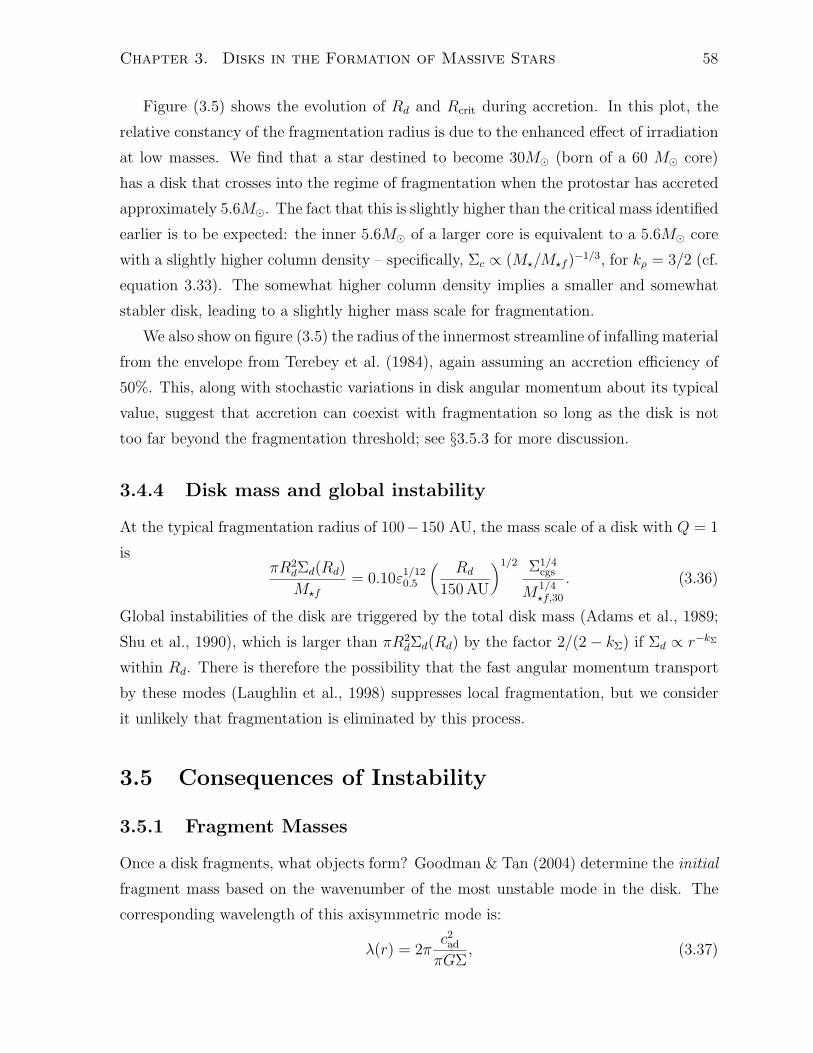
Chapter 3. Disks in the Formation of Massive Stars 58
Figure (3.5) shows the evolution of Rd and Rcrit during accretion. In this plot, the
relative constancy of the fragmentation radius is due to the enhanced e!ect of irradiation
at low masses. We find that a star destined to become 30M" (born of a 60 M" core)
has a disk that crosses into the regime of fragmentation when the protostar has accreted
approximately 5.6M". The fact that this is slightly higher than the critical mass identified
earlier is to be expected: the inner 5.6M" of a larger core is equivalent to a 5.6M" core
with a slightly higher column density – specifically, $c % (M"/M"f )!1/3, for k# = 3/2 (cf.
equation 3.33). The somewhat higher column density implies a smaller and somewhat
stabler disk, leading to a slightly higher mass scale for fragmentation.
We also show on figure (3.5) the radius of the innermost streamline of infalling material
from the envelope from Terebey et al. (1984), again assuming an accretion e#ciency of
50%. This, along with stochastic variations in disk angular momentum about its typical
value, suggest that accretion can coexist with fragmentation so long as the disk is not
too far beyond the fragmentation threshold; see §3.5.3 for more discussion.
3.4.4 Disk mass and global instability
At the typical fragmentation radius of 100&150 AU, the mass scale of a disk with Q = 1
is.R2
d$d(Rd)
M"f= 0.10%1/12
0.5
'Rd
150 AU
(1/2 $1/4cgs
M1/4"f,30
. (3.36)
Global instabilities of the disk are triggered by the total disk mass (Adams et al., 1989;
Shu et al., 1990), which is larger than .R2d$d(Rd) by the factor 2/(2& k!) if $d % r!k!
within Rd. There is therefore the possibility that the fast angular momentum transport
by these modes (Laughlin et al., 1998) suppresses local fragmentation, but we consider
it unlikely that fragmentation is eliminated by this process.
3.5 Consequences of Instability
3.5.1 Fragment Masses
Once a disk fragments, what objects form? Goodman & Tan (2004) determine the initial
fragment mass based on the wavenumber of the most unstable mode in the disk. The
corresponding wavelength of this axisymmetric mode is:
#(r) = 2.c2ad
.G$, (3.37)

Chapter 3. Disks in the Formation of Massive Stars 59
0.1 1 10
1
10
M! (M!)
R(A
U)
Typical
disk
radi
us
Inne
r stre
amlin
e
Maximum stable radius
Viscosity Irradiation
Figure 3.5: Growth of disk and critical radius with the mass of a protostar accreting
toward 30M" in the fiducial core collapse model. In addition to the expected disk radius,
we show the splashdown radius of the inner infall streamline, calculated assuming % = 0.5.

Chapter 3. Disks in the Formation of Massive Stars 60
where $ and cs are both functions of radius within the disk. Assuming that the fragment
has comparable dimension azimuthally, the corresponding mass scale is (Goodman &
Tan, 2004)
Mfrag = #2$
=4.
%
c3ad
GQ, (3.38)
i.e., roughly the amount of mass accreted in 2Q orbits. We assume fragmentation only
occurs when Q * 1. We consider our rather idealized estimate of Mfrag uncertain by
at least a factor of two. In reality the initial mass is likely a stochastic variable, best
determined from numerical simulations (R. Rafikov, private communication).
Once a fragment forms, its growth is controlled by accretion of surrounding gas, mi-
gration through the disk, and collisional or gravitational interaction with other fragments.
Rather than address these questions in detail, we will draw preliminary conclusions by
comparing Mfrag to two critical scales: the gap opening mass Mgap and the isolation mass
Miso. A fundamental uncertainty is the state of the gas disk: again, we assume Q = 1.
When the gravitational torques exerted on the disk by the fragment exceed viscous
torques, a gap opens around the fragment. Rafikov (2002) estimates
Mgap =2c3
ad
3%G
(
0.043
= 0.37(/0.30
QMfrag. (3.39)
Since this is less than Mfrag, and gets even smaller if the disk viscosity goes down and
thus cooling time goes up relative to the critical state in the Gammie (2001) simulations,
we expect fragments to open gaps immediately.
Gap opening slows but does not necessarily end accretion (Artymowicz & Lubow,
1996). A possible limit to growth is set by the point at which the fragment accretes
all the mass within its Hill radius (e.g., Goodman & Tan, 2004, but see Artymowicz &
Lubow). This defines the isolation mass
Miso(r) ((2.fHr2$)3/2
9M1/2"
(3.40)
where fH . 3.5.
Figure (3.6) compares the initial, gap opening, and isolation masses for a range of
M"f , evaluated at Rcrit near the end of core accretion (in the fiducial core model). Because

Chapter 3. Disks in the Formation of Massive Stars 61
10 100
0.1
1
10
Initial fragment mass
Isolation mass
Gap opening mass
M! (M!)
Mfr
ag(M!
)
Figure 3.6: Our estimate of the initial fragment mass, compared to the gap opening
mass and isolation mass, at the end of accretion in the fiducial core collapse model. We
truncate the calculation where dust sublimation in the envelope makes the critical radius
determination uncertain.
gap opening slows accretion, we expect the masses of disk-born stars to resemble Mfrag
more than Miso. In this case they will be low-mass stars of order 0.2–0.4 M".
Fragmentation tends to set in at $ 100 & 200 AU, as we noted in §3.2.4. However
gap-opening fragments should be swept inward if disk accretion continues; only a single
disk mass of accretion is required to bring them in to the central object. If they move
inward by about a factor of 30, they will be within a few stellar radii at carbon ignition
(Webbink, 1985). As candidates for mass transfer and common-envelope evolution, such
objects can serve as reservoirs of matter and angular momentum for the relic of the
central star’s supernova explosion.

Chapter 3. Disks in the Formation of Massive Stars 62
3.5.2 Observability of Disk-Born Stars
We have predicted that stars with extended protostellar disks will produce low mass (M5–
G5) companions. Thus we would expect many O stars, and perhaps some early B stars,
to have multiple coplanar companions at separations of order <$ 100&200 AU, depending
on the amount of migration that occurs following formation. In the closest clusters, for
example, Orion, this correspondes to an angular separation of approximately 0.4$$ and
an apparent bolometric magnitude di!erence of, at a minimum, $ 13 magnitudes. This
implies that even in K-band with an AO system such as that of VLT, such objects would
be di#cult to observe (M. Ahmic, private communication). Similarly, the combination
of AO with a coronograph (e.g. the Lyot coronograph on AEOS) can provide a dynamic
range of up to up to 8 H-band magnitudes at a few hunderd mas, which is still too small
to detect the aforementioned companions (Hinkley et al., 2007). If not detectable during
the main sequence life of the primary star, the presence of such companions might be
observable via binary interaction once the primary evolves.
3.5.3 Disk E"ciency
If a 30M" star will su!er disk fragmentation early in its accretion, as we estimated in
§3.4.3 on the basis of the turbulent core model, then we must address how this might
impact subsequent accretion. One possibility is that gap-opening fragments will be swept
inward to the central star, in which case its final mass will be una!ected. This outcome
resembles the scenario outlined by Levin (2003) for gravitationally unstable AGN accre-
tion. Alternatively, Tan & Blackman (2005) suggest low-luminosity AGN may be starved
of gas by fragmentation.
In the latter scenario, a strongly unstable disk will have a low disk e!ciency, %d -M"/M"d. We can estimate %d in the limit that none of the gas entering an unstable region
of the disk ultimately accretes onto the star. The splashdown radius of the innermost
streamline was estimated in expression (3.12). Given that outflow removes matter from
the inner streamlines, and that fragmentation removes it from the outer portions of the
disk, the fraction of mass that successfully accretes (after striking the disk) is
%d = 1& %!1
#
1&'1& Rcrit
Rd
(1/2$
. (3.41)
Of course, this expression is only applicable when it yields 0 ' %d ' 1, i.e., when the disk
is partly but not wholly unstable.

Chapter 3. Disks in the Formation of Massive Stars 63
Two complications arise when evaluating equation (3.41). First, the critical radius
Rcrit must be calculated using the mass accretion rate outside of itself. Second, recall
that the angular momentum of infalling gas derives from its initial turbulent velocity
and is likely to vary in direction and magnitude. The fluctuations of j were estimated
by the distribution fj, which appeared in equation (3.25). Accounting for both of these
e!ects, we find that accretion can continue even in an actively unstable disk. For 30M",
we find that the infall streamline remains within the stable disk radius through the end
of accretion. Even if all the gas entering a fragmenting region is consumed, this need
not fully starve the central object. However, the tendency to fragment becomes much
stronger for more massive stars. This is especially true for those (M"f $ 110M", from
§3.4) that accrete rapidly enough that their disks are destabilized by the drop in dust
opacity.
In reality, we expect some gas to accrete through the unstable region. A rough upper
limit would be to adopt the accretion rate for a Toomre-critical (Q = 1) state, and assume
that any surplus is consumed by fragmentation. In this case, the central accretion rate
would be limited by the temperature of the coldest region of the disk (according to
eq. 3.4). Numerical simulations will ultimately be required to quantify the behaviour of
Toomre-unstable disks.
Furthermore, there are numerous feedback mechanisms that have not been addressed.
For example, if fragmentation halts accretion, this could change the outflow power, the
shape of the outflow and infall cavity and thus the heating of the disk by reprocessed
starlight. This interplay will be investigated in future work.
3.6 Discussion
Our primary conclusion (§3.2.4) is that massive-protostar disks that accrete more slowly
than $ 1.7) 10!3M" yr!1 are subject to fragmentation at disk radii beyond about 150
AU. This critical radius is set primarily by the viscous heating of the disk midplane as
it accretes, with reprocessed starlight playing an equal or secondary role for most stellar
masses. As all the disks we consider are optically thick, the critical radius depends on
the Rosseland opacity law )R(T ) within dusty disk gas.
Comparing to our conservative estimate of the disk radius in the McKee & Tan (2003)
model for massive star formation by the collapse of turbulent cores (§3.3), we find that
fragmentation is marginal for stars accreting four to 15 solar masses; higher-mass stars are

Chapter 3. Disks in the Formation of Massive Stars 64
increasingly a(icted by disk fragmentation. Although the mass at which fragmentation
sets in is sensitive to our somewhat uncertain fragmentation criterion (§3.2.1) and angular
momentum calculation (§4.3.4 and the Appendix), we have been conservative in five
ways: (1) by adopting a fragmentation temperature lower than that implied by the
Rice et al. (2005) simulations; (2) by adopting a low estimate of the specific angular
momentum that determines the disk radius; (3) by adopting a relatively opaque model
for the disk’s Rosseland opacity; (4) by ignoring the shielding e!ect of a moderately
opaque infall envelope, and (5) by adopting a low estimate for the cooling time, and
a hard equation of state. All of these approximations should, if anything, lead us to
underestimate the prevalence of disk fragmentation. Along with the existence of turbulent
fluctuations in j (§3.4), these points ensure that some massive stars above $ 10M"
experience disk fragmentation. As noted in §3.4.4, we cannot rule out the possibility
that global instabilities flush disk material fast enough to suppress fragmentation, but
we consider it unlikely that this prevents all fragmentation.
We therefore expect multiple, coplanar, low-mass (M5 to G5, §3.5.1) companions
to form around many O (and some B) stars. Given initial separations of order 100-
200 AU, their photospheric emission is not observable with present techniques. Disk
migration, followed by mass transfer or common-envelope evolution, may however make
them evident as the primary evolves (§3.5.2).
Even when disks fragment, we expect some accretion onto the central star – if only
because of material that falls within the fragmentation radius (§3.5.3). Although we
cannot yet quantify the disk e#ciency parameter %d, we expect it to be significantly less
than unity for those early O stars (M"f>$ 50M") whose disks are most prone to fragment.
3.6.1 Imprint on the initial mass function
The stabilizing e!ect of viscous heating is absent in disks that accrete more rapidly than
1.7 ) 10!3M" yr!1, thanks to a sharp drop in dust opacity at $ 1050 K (see §3.4). As
this a!ects stars of mass greater than 87(tacc/105yr)M", or about 110 M" in the fiducial
core model, it may be related to the cuto! of the initial mass function (IMF) at about
120 M".
Several other explanations for this cuto! have been proposed, all involving the in-
creasing bolometric luminosity, ionizing luminosity, or outflow force emitted by the cen-
tral star. Starvation by disk fragmentation has the distinctive feature that it becomes

Chapter 3. Disks in the Formation of Massive Stars 65
much more severe at a specific accretion rate. For this reason we expect it to produce a
sharper IMF cuto!. (The transition to super-Eddington luminosities could also produce
a sharp cuto!, but Krumholz et al. 2005 argue that this can be overcome by asymmetric
radiation transfer.)
Note also that disk accretion is destabilized by rapid accretion, whereas rapid accre-
tion quenches the e!ects of direct photon force and of the ionizing radiation (Wolfire &
Cassinelli, 1987). Disk fragmentation may close an avenue by which very massive stars
would otherwise form.
3.6.2 Proto-binary disks
Pinsonneault & Stanek (2006) state that close massive binaries < 10 year periods) are
more likely to have nearly equal masses. More generally, the binarity fraction overall
among massive stars is higher than their low mass counterparts (1.5 versus 0.5, Bally
et al. (2005)). Due to the high fraction of roughly equal mass binaires, their e!ect
on disk dynamics must be addressed in future work. Moreover, the stellar densities in
regions of HMSF are high, suggesting that other cluster stars might be close enough to
interfere with disks stretching out to $ 100 AU (Bate et al., 2003). It is not currently
clear whether disk accretion can preferentially grow a low-mass companion until its mass
rivals that of the primary star, as Artymowicz & Lubow (1996) suggest. If so, then disk
fragmentation may be relevant in the production of equal-mass binaries; if not, they must
form by another mechanism. In any case, the multiplicity of the center of gravity should
be accounted for in future work. It seems unlikely, though, that a binary with $ 10 year
period will stabilize the fragmenting regions whose periods are >$ 300 years.
3.7 Appendix
We present here an estimate of the angular momentum of cores initially supported by
turbulent motions, generalizing the results of ML05 to arbitrary line width-size relations.
The analytical treatment of this problem rests on several idealizations about turbulent
velocities: (1) that they are isotropic and homogeneous; and (2) that the Cartesian
velocity components are neither correlated with each other, nor (to any appreciable
degree) with density fluctuations. For simplicity we also assume (3) that the core density
profile is spherically symmetric and can be captured in a single function '(r). When

Chapter 3. Disks in the Formation of Massive Stars 66
evaluating our formulae we assume (4) that the velocity di!erence between two points
scales as a power of their separation, and (5), for the purpose of computing fluctuations,
that the velocity components are Gaussian random fields.
One might object that condition (1) is inconsistent with the turbulent support of an
inhomogeneous density profile. Consider, however, that if the core profile is a power law
'(r) % r!k! , then the turbulent line width must scale as !(r) % r$ where
& = 1& k#/2. (3.42)
A velocity field with this scaling is consistent with our conditions (1), (2), and (4) if
"[vi(r1)& vj(r2)]2# = k|r1 & r2|2$*ij (3.43)
where angle brackets represent an ensemble average and k is a normalization constant
related to the virial parameter (. ML05 considered the case & = 1/2 appropriate for giant
molecular clouds (k# = 1); we generalize their formulae to other values of &, including
the fiducial value & = 1/4 corresponding to k# = 3/2.
Our goal is to compute the expectation value and dispersion of the core specific
angular momentum j, normalized to Rc! where ! is the one-dimensional line width of
the core. We find that, under our assumptions,
"j2# = &* * d3r1'(r1)
M
d3r2'(r2)
Mr1 · r2"[vx(r1)& vx(r2)]
2# (3.44)
and that
"!2# =1
2
* * d3r1'(r1)
M
d3r2'(r2)
M"[vx(r1)& vx(r2)]
2# (3.45)
where M ="
'd3r and all integrals are restricted to the region of interest (typically the
core interior). These equations, which we will prove below, agree with the formulae in
ML05’s Appendix but allow "[vx(r1) & vx(r2)]2# to be an arbitrary function of |r1 & r2|.It is important to note that the two formulae are identical up to the factor &2r1 · r2 in
the integrand. The negative sign in equation (3.44) ensures that "j2# is positive, since
"[vx(r1)&vx(r2)]2# takes higher values when |r1&r2| is large, hence when r1 ·r2 is negative.
To evaluate equations (3.44) and (3.45) we make use of spherical symmetry and
impose equation (3.43) for the velocity correlations. Defining µ = r1 · r2/(r1r2) as the
cosine of the angle between r1 and r2,
"j2# = &k* R
0dr14.r2
1
'(r1)
M
* R
0dr22.r2
2
'(r2)
Mr1r2
3r21 + r2
2
4$* 1
!1dµ (1& qµ)$ µ

Chapter 3. Disks in the Formation of Massive Stars 67
Profile & = 1/4 & = 1/2
turbulent core 0.2704 0.4206
critical Bonnor-Ebert sphere 0.2730 0.3828
uniform region (k# = 0) 0.3430 0.4714
thin shell 0.4714 0.6324
Table 3.4: Values of "j2#1/2/(R"!2#1/2) in our model for turbulent angular momentum.
=2.2k
M2
* R
0dr1
* R
0dr2
3r21 + r2
2
42+$r1r2'(r1)'(r2)) (3.46)
#(1 + q)$+2 & (1& q)$+2
& + 2& (1 + q)$+1 & (1& q)$+1
& + 1
$
and
"!2# =1
2k
* R
0dr14.r2
1
'(r1)
M
* R
0dr22.r2
2
'(r2)
M
3r21 + r2
2
4$* 1
!1dµ (1& qµ)$
=2.2k
M2
* R
0dr1
* R
0dr2
3r21 + r2
2
41+$r1r2'(r1)'(r2)) (3.47)
#(1 + q)$+1 & (1& q)$+1
& + 1
$
where q = 2r1r2/(r21 + r2
2), as in ML05. Table 3.7 and figure 3.7 provide values of
"j2#1/2/(R"!2#1/2) for several density profiles, both for the internal spectrum given by
equation (3.42), and for & = 1/2, which may better represent the background spectrum.
Figure 3.7 plots the ratio "j2#1/2/(R"!2#1/2) as given by equations (3.46) and (3.47)
for a turbulent core profile, a critical Bonnor-Ebert sphere, and a thin shell. The results
are very close to power laws in &:
"j2#1/2
R"!2#1/2.
/00000001
00000002
0.655&0.638 singular turbulent core
0.537&0.488 critical Bonnor& Ebert sphere
0.648&0.459 uniform& density sphere
0.849&0.424 thin shell.
(3.48)
The spin parameter 3j makes reference to the velocity dispersion !(R) at radius R,
rather than the mean velocity dispersion "!2#1/2 within R. For this we use the scaling
!2 % GM/r %M2$/(3!k!) to derive
!(R)2
"!2# = 1 +2&
3& k#.

Chapter 3. Disks in the Formation of Massive Stars 68
0 0.1 0.2 0.3 0.4 0.50
0.1
0.2
0.3
0.4
0.5
0.6
0.7
Line width-size exponent !
Dim
ensi
onle
ssro
tation
:! j2
" 1/2/
# R! "
2" 1
/2$
Singular turbulent c
ore
Thin shell
Critical Bonnor!
Ebert sphere
Uniform sphere
Figure 3.7: Values of "j2#1/2/(R"!2#1/2) evaluated for turbulence with line width-size
exponent & and three relevant density profiles. For hydrostatic turbulent cores, ' %r!2(1!$).
With this correction factor accounted for, 3j/fj is still very close to a power law of &:
3j
fj.
/0001
0002
0.504&0.552 singular turbulent core
0.987&0.651 uniform& density region
0.849&0.424 thin shell.
(3.49)
(The last line is unchanged, as there is no correction for a thin shell.) These formulae
were quoted in §4.3.4.
We now return to the derivation of equation (3.44); equation (3.45) is treated below.
The z component of the specific angular momentum of the core is
j2z =
*d3r1
*d3r2
'1
M(x1vy1 & y1vx1)
'2
M(x2vy2 & y2vx2)
=1
M2
*d3r1
*d3r2'1'2(x1x2vy1vy2 + y1y2vx1vx2 & x1y2vy1vx2 & y1x2vx1vy2);(3.50)
here, as below, we use subscripts 1 and 2 to indicate functions of r1 and r2, i.e., '1 = '(r1).
On ensemble averaging of the second line, the last two terms in equation (3.50) become
zero thanks to the *ij in equation (3.43). The first two terms are equal, thanks to spherical
symmetry; thus
"j2z # =
2
M2
*d3r1
*d3r2'1'2x1x2"vy1vy2#. (3.51)

Chapter 3. Disks in the Formation of Massive Stars 69
Spherical symmetry allows us to replace x1x2 with r1 · r2/3 and j2z with j2/3, so
"j2# =2
M2
*d3r1
*d3r2'1'2r1 · r2"vy1vy2#
=1
M2
*d3r1
*d3r2'1'2r1 · r2
3"v2
y1#+ "v2y2# & "(vy1 & vy2)
2#4. (3.52)
The first two terms within the brackets are zero, as spherical symmetry requires them to
be even in the space coordinates while r1 · r2 is odd; the surviving term yields equation
(3.44).
To prove equation (3.45) we write
M!2 =*
d3r'(r)(vx & vx)2 =
*d3r'(r)(v2
x & v2x) (3.53)
where v ="v'(r)/Md3r is the center of mass velocity. In equation (3.50) we replace v2
x
with" "
v1 · v2('1/M)('2/M)d3r1d3r2, and we bring the first term into similar form by
multiplying it by"('2/M)d3r2 = 1:
M!2 =*
d3r1
*d3r2'1'2vx1(vx1 & vx2)
=1
2
*d3r1
*d3r2'1'2(vx1 & vx2)
2. (3.54)
The second line follows from the first by noting that the integral is antisymmetric under
interchange of r1 and r2. When averaged, it yields equation (3.45).

Chapter 4
Global Models of Young, Massive
Protostellar Disks
A version of this chapter has been published in The Astrophysical Journal as “Global
Models for the Evolution of Embedded, Accreting Protostellar Disks”, Kratter, K. M.,
Matzner, C. D., and Krumholz, M. R., vol. 681, pp375-390, 2008. Reproduced by per-
mission of the AAS.
4.1 Introduction
Having determined that disks around massive are susceptible to fragmentation, we now
explore the propensity of disks to fragment across a broader mass range. Moreover, we
now employ a more sophisticated model for accretion driven by gravitational instability
and the magnetorotational instability in order to survey the conditions in protostellar
disks as a function of mass and time.
A young star system’s visible T Tauri or Herbig stage is preceded by a deeply en-
shrouded phase of rapid accretion in which its character – multiplicity, disk properties,
and tendency to form planets – is first forged. Due to the high obscuration characteristic
of this phase, disks are accessible primarily via radio and submillimeter observations,
and such techniques provide limited sensitivity and angular resolution compared to what
can be achieved for T Tauri and Herbig AE star disks using shorter wavelengths. Our
knowledge of massive protostellar disks is particularly limited by this problem, since they
do not have a significant unobscured phase, probably due to the destructive e!ects of
ionizing radiation. These di#culties are compounded by the fact that massive stars form
70

Chapter 4. Global Models of Young, Massive Protostellar Disks 71
more rarely, and therefore tend to lie farther away. Detections of rotation and infall in
a few systems hint at the presence of disks during the embedded phase, but are only
preliminary (see recent reviews by Cesaroni et al. 2006, 2007, Beuther 2006, and Beuther
et al. 2007).
While our knowledge of the embedded phase today is limited, it will soon come into
sharp focus as new instruments such as the Expanded Very Large Array (EVLA) and
Atacama Large Millimeter Array (ALMA) become operational. In order to predict what
these telescopes will discover about the formation of stars across a very broad mass range,
$ 1 & 120M", we present evolutionary models of star-disk systems reacting to infall at
very high rates. We concentrate our e!orts on the physical processes that control disk
evolution, such as the torque from a turbulent infall, the reprocessing of starlight by the
infall envelope, and the character of the self-gravitational instabilities. The disk itself
we model with a highly simplified, single-zone treatment. Although multidimensional
simulations provide a much more detailed view of disk formation and evolution during
the embedded phase (e.g. Goodwin et al., 2004; Krumholz et al., 2007b), their high com-
putational cost and the limited range of physical processes they include mean that these
simulations can explore only small regions of parameter space. They cannot easily make
predictions across a broad range of stellar mass scales and evolutionary times. In contrast,
our semi-analytic approach permits us to incorporate more physical e!ects and explore
the consequences of environmental parameters more rapidly, and in a more systematic
way. This serves two complementary ends: the theoretical goal of understanding angular
momentum transport and fragmentation in the embedded phase, and the observational
goal of making concrete predictions about the properties of young, massive disks.
Although we include a range of physical processes in our models; the most impor-
tant in driving the evolution of embedded disks in our calculations is self-gravity. Self-
gravity plays a central role in mediating angular momentum transport and triggering
fragmentation into a binary or multiple system. Its importance in star formation has long
been recognized (Larson, 1984), and our study is preceded by evolutionary calculations
which incorporate accretion and self-gravity into one-dimensional (Lin & Pringle, 1987,
1990; Nakamoto & Nakagawa, 1994, 1995; Hueso & Guillot, 2005) and two-dimensional
(Vorobyov & Basu, 2005, 2006) simulations. Although lower in resolution, our approach
is distinguished from these works in several ways:
i. In contrast to all one-dimensional calculations to date, we account for the de-

Chapter 4. Global Models of Young, Massive Protostellar Disks 72
pendence of gravitational torques on the disk-to-total mass ratio in addition to
Toomre’s instability parameter.
ii. We consider the possibility that disks will fragment if they become su#ciently
unstable.
iii. We consider fluctuations of the vector angular momentum in the infall due to
realistic turbulence in the collapsing cloud core.
iv. We employ a realistic model for the irradiation of the disk midplane, in which
starlight is reprocessed at the inner wall of an outflow cavity while inflow is occur-
ring.
v. We survey the conditions of intermediate-mass and massive star formation, rather
than focusing exclusively on conditions in nearby low-mass star forming regions
such as Taurus.
The first of these is important for all protostellar disks, since the disk mass is never
negligible when the Toomre parameter is small. Features (ii) and (iii) are of primary
importance in the formation of massive stars, which accrete from strongly turbulent
regions (Myers & Fuller, 1992; McLaughlin & Pudritz, 1997) and which are likely to
undergo disk fragmentation (Kratter & Matzner 2006, hereafter KM06). Irradiation is
most important for low-mass stars, whose disks it strongly stabilizes (Matzner & Levin,
2005), but it remains significant in massive star formation as well.
In §4.2 we outline our model for the infall rate of matter and angular momentum. We
develop a model for disk accretion and fragmentation in §4.3. In §4.4 we define the key
environmental variables that control protostellar disk evolution and sketch a qualitative
evolutionary sequence based on their fiducial values. In §4.5 we present the results for
our fiducial case, and explore the e!ect of varying our parameters. In §4.6 we discuss
the observable predictions that our model makes, and finally in § 4.7 we summarize our
main results.
4.2 Infall onto Disks
Since we are interested in the behavior of a disk that is subject to strong perturbations
from its environment, we begin building our model by constructing a prescription for

Chapter 4. Global Models of Young, Massive Protostellar Disks 73
the infall of matter and angular momentum onto a disk. This accretion comes from
a background “core” (Shu, 1977a; McLaughlin & Pudritz, 1997; McKee & Tan, 2003),
whose properties and interaction with a disk we discuss in this section.
4.2.1 Star Formation By Core Collapse
We model the accretion of mass and angular momentum using the two-component core
model of McKee & Tan (2003), which is a generalization of the TNT (thermal plus non-
thermal) model of Myers & Fuller (1992). In this model, which we summarize here for
convenience, the density distribution within a core follows a two-component power law
distribution
' = 's
'Rc
r
(!k!
+c2s,c
2.Gr2, (4.1)
where Rc is the outer radius of the core, cs,c is the thermal sound speed within it (assumed
to be constant), and 's is the density at the core’s surface. We follow McKee & Tan
(2003) in adopting k# = 1.5 as the fiducial value of the turbulence-supported density
index. Physically, the first term describes an envelope supported primarily by turbulent
motions, while the second describes a thermally-supported region at its center. A model
of this sort is fully specified in terms of the three parameters: the core mass
Mc =4.
3& k#'sR
3c + 2
c2s,cRc
G, (4.2)
surface density
$c =Mc
.R2c
, (4.3)
and temperature
Tc =m
kBc2s,c, (4.4)
where m = 3.9 ) 10!24 g is the mean particle mass in a gas of molecular hydrogen and
helium mixed in the standard cosmic abundance. Observed regions of star formation
contain cores with masses $ 1 & 100 M", surface densities $c ( 0.03 & 1 g cm!2, and
temperatures of 10 to 50 K (Johnstone et al., 2001; Plume et al., 1997).
The core is taken to be in approximate hydrostatic balance initially, and this condition
specifies the required level of turbulent support. The non-thermal velocity dispersion in
the shell at radius r is
!(r)2 =2.
3$B(k# & 1)
GM(r)
r& c2
s,c (4.5)

Chapter 4. Global Models of Young, Massive Protostellar Disks 74
where M(r) is the mass at radii of r or less and $B . 2.8 approximately accounts for
the magnetic contribution to the total pressure. Except when M(r), 1 M" or $c < 0.1
g cm!2, the first term is much larger than the second, so that the velocity dispersion is
primarily non-thermal.
Core collapse commences at time zero, and a mass shell initially at radius r falls
onto the disk in a time comparable to the free fall time evaluated at its initial density,
t"(r) = [3./32G'(r)]1/2. In practice, we use the McKee & Tan (2003) accretion rate
approximation to determine M on to the star-disk system as a function of the total core
mass and the current amount of mass that has accreted:
Min (%
$#M#f
t",s
& 5
6%
M#d
M#f
&2q
+
%$#th$#nth
&2 %%Mth
M#f
&2q7
81/2
, (4.6)
where M#f is the final disk plus stellar mass, M#d is the current disk plus stellar mass,
t",s is the free-fall time evaluated at the core surface (i.e. at ' = '(Rc)),
q =3(2& k#)
2(3& k#), (4.7)
Mth = 10!3.1'
T
20 K
(3%
30%M"
M#f
&1/2
$!3/2c,0 M", (4.8)
$c,0 = $c/(g cm!2), and $#, $#nth, and $#th are constants of order unity that depend on
the polytropic index and magnetic field strength. The e#ciency factor
% =M#f
Mc(4.9)
represents the fraction of the core mass that lands on the star-disk system rather than
being blown out by protostellar outflows. We again follow McKee & Tan (2003) in
adopting % = 0.5, a value typical of low-mass star formation (Matzner & McKee, 2000).
4.2.2 Angular Momentum of the Infalling Material
Equation (4.6) gives the mass infall rate Min(t) from the core as a function of time.
The second component of our core model is to specify the corresponding rate of angular
momentum infall Jin(t). We compute this in several steps. First, we approximate the
vector specific angular momentum j(r) averaged over a shell of material at radius r as
described below. Then we compute M(t) -" t0 Min(t$)/4 dt$, the total mass from the core
that has either fallen onto the star-disk system or been ejected at time t. From the

Chapter 4. Global Models of Young, Massive Protostellar Disks 75
core density profile (equation 4.1) we also compute M(r) -" r0 4.r$2'(r$) dr$, the mass of
the initial core enclosed within radius r. Assuming the core accretes inside-out, we set
M(r) = M(t) and solve for r(t), which gives the initial radius r of the shell of mass that
arrives at the star-disk system at time t. Assuming that the specific angular momentum
of the gas does not change before it reaches the disk, the angular momentum accretion
rate is then simply given by Jin(t) = Min(t)j(r(t)).
The remaining step is to specify how we estimate j(r). Star forming cores are often
modeled as solid body rotators characterized by the ratio & of rotational to gravitational
energy, but we adopt a more realistic model in which turbulent fluctuations a!ect the
infalling gas. Following Burkert & Bodenheimer (2000), Fisher (2004), Matzner & Levin
(2005) and KM06, we assume that the observed angular momenta of cores (Goodman
et al., 1993) can be modeled using an idealized turbulent velocity field. Using the method
of Dubinski et al. (1995), we generate a numerical realization of an isotropic, homoge-
neous, Gaussian random velocity field v(r). We require that the power spectrum P (k) of
this turbulent field reproduce the scalings required by turbulent support against gravity:
!(r)2 % GM(r)/r % r2!k! at large radii, so that !(r) % r1/4 for k# = 3/2. Parseval’s
theorem or dimensional analysis then require P (k) % k!3/2.
We note that numerical simulations of supersonic turbulence consistently show the
steeper spectral index &2 (Porter et al., 1992) which is understood as the spectrum of
an individual shock and as the exact limit of Burgers turbulence. Matzner (2007) and
Nakamura & Li (2007) have shown that a shallower index is expected when turbulence
is driven by protostellar outflows, however, and our chosen power spectrum is consistent
with the line width-size relation for massive cores (e.g., Caselli & Myers, 1995; Plume
et al., 1997). Our homogeneous velocity field is surely an idealization, but not a grave
one.
After scaling our numerical domain to match the core radius Rc, we normalize v such
that the one-dimensional velocity dispersion of a spherical shell with this radius equals
!(r) defined in equation (4.5). In practice we fit Rc within a 2563 section of a 10243
grid of velocities, because periodicity causes artifacts on scales larger than about 1/4 of
the box size. From this field we calculate the specific angular momentum j = r ) v at
every point and the mean specific angular momentum j(r) in a shell at radius r. Note
that KM06 calculate the expected magnitude and dispersion of j(r) for velocity fields of
precisely this type; our results agree with their predictions to about 50%, which is within
the scatter they predict.

Chapter 4. Global Models of Young, Massive Protostellar Disks 76
4.3 Dynamics of the disk
4.3.1 Approach to disk evolution
Given the rate at which mass and angular momentum accrete, we must calculate the
reaction of the disk. At any given time, our star-plus-disk system is characterized by the
disk mass Md, the central star mass M#, and the total angular momentum content of the
disk Jd. Given these quantities, and the rates of mass and angular momentum infall Min
and Jin, we wish to compute the time rate of changes Md, M#, and Jd.
Using the separation between the thermal, orbital, and accretion timescales, we as-
sume our disks are in a thermal steady state and draining at a rate determined by their
current global parameters. We shall later refer to this as the assumption of thermal and
mechanical equilibrium.
In § 4.3.2, we estimate the disk accretion rate onto the central star due to various
angular momentum transport mechanisms. In § 4.3.3 we discuss thermal equilibrium in
the disk, which together with the aforementioned condition of mechanical equilibrium
allows us to self-consistently compute the accretion rate from the disk to the star M#. In
§ 4.3.4 we describe the corresponding angular momentum evolution Jd. Finally, in § 4.3.5
and § 4.3.6, we discuss our prescriptions for disk fragmentation and binary formation.
It is helpful before proceeding to define two dimensionless parameters that character-
ize the strength of the disk’s self-gravity. These are the disk-to-total mass ratio
µ =Md
Md + M#(4.10)
and Toomre’s (1964) instability parameter
Q =cs)
.G$d, (4.11)
where ) is the radial epicyclic frequency, cs speed of density waves, and $d is the disk’s
mass surface density. In practice we evaluate Q using )* % = (GMtot/R3d)
1/2, the total
orbital frequency, since the di!erence between them is only marginally significant even
when the disk mass is quite large. Here Rd = j2d/GMtot. We also approximate cs using the
isothermal sound speed. To characterize gravitational instability, we use the minimum
value of Q – the value at Rd, the outer boundary of our active disk. In this evaluation we
assume a profile $d % r!1 (a choice we justify in § 4.3.4) so that $d(Rd) = Md/(2.R2d),
and we evaluate cs and % at the edge of the disk.

Chapter 4. Global Models of Young, Massive Protostellar Disks 77
We base our models on the fundamental assumption that the self-gravitational be-
havior of an accretion disk depends primarily on the structural parameters µ and Q –
so that its evolution is controlled by heating and cooling (§ 4.3.3), which alter Q, and
accretion onto and through the disk, which alters µ. This approach permits us to treat
the disk’s mechanical and thermal properties separately, before combining them into a
model for its evolution. This division also guides our use of published work, since it
implies that simulations with adiabatic equations of state and those with an imposed
cooling rate may be combined into a mechanical model for disk evolution, which we may
then use to model irradiated protostellar disks. Finally, it prompts us to treat the onset
of disk fragmentation and disk fission as boundaries in the space of µ and Q, rather
than in terms of a critical cooling rate (which is the natural and conventional description
for simulations that include cooling but not irradiation). In § 4.3.5 we argue that these
descriptions are e!ectively equivalent.
Models based on this assumption are guaranteed to be somewhat approximate, be-
cause a disk’s mechanical evolution must, at some level, reflect additional parameters: its
geometry, its equation of state, the specifics of its heating and cooling processes, and the
magnitude of external perturbations (like tides), to name a few. However we expect our
results to be valid, both because we believe that µ and Q are indeed the most significant
parameters for gravitational instability, and because our model is calibrated to realistic
numerical models. Additional simulations will be required to test this approach.
4.3.2 Angular Momentum Transport and Disk Accretion
A key element of our model is a prescription for angular momentum transport and the rate
M# at which matter accretes onto the central star – or more specifically, the dimensionless
rate M#/(Md%). In practice we first construct a model for an e!ective Shakura & Sunyaev
( parameter, which we define through the steady-state relation
M# =3(c3
s
GQ(4.12)
so thatM#
Md%=
3(Q2
8µ2, (4.13)
where the factor of of 3/8 comes from the assumption that the disk surface density falls as
r!1. We do not mean to imply by this that transport induced by gravitational instability

Chapter 4. Global Models of Young, Massive Protostellar Disks 78
is purely local (Balbus & Papaloizou, 1999), although this does appear to be the case for
su#ciently thin and light disks (Gammie, 2001; Lodato & Rice, 2005).
We divide ( into two contributions: (MRI, due to the magnetorotational instability
(MRI), and (GI, due to gravitational instability. In keeping with the strategy described
in § 4.3.1, we consider (GI to be a pure function of µ and Q. We combine it and the MRI
contribution linearly:
( = (GI + (MRI . (4.14)
We create our model for (GI(Q, µ) using results from the simulations of Laughlin &
Rozyczka (1996), Rice et al. (2003), Lodato & Rice (2004), Lodato & Rice (2005) and
Gammie (2001). We adopt a constant value for (MRI , as discussed below.
Overview of Simulations
The three sets of simulations span a large fraction of our parameter space in Q and µ. The
global disk simulations of Laughlin & Rozyczka (1996) explore Q > 1 and non-negligible
values of µ using a two-dimensional hydrodynamic, self-gravity code; they supress local
fragmentation by imposing an adiabatic equation of state. The simulations of Gammie
(2001) represent the limit µ* 0, for values of Q which approach unity from above, and
are most directly applicable to quasar disks.
Gammie imposes cooling with a fixed cooling time, 1c, which is proportional to the
orbital time. He finds a regime of steady gravity-induced turbulence, for disks that
cool over many orbits. If 1c is too short (< 3%!1), however, the disk fragments as
Q drops below unity. The disk viscosity is highest at the boundary of fragmentation.
Angular momentum transport in this regime is quite local, with an e!ective value of (
that is inversely proportional to the cooling rate. Our third source is the global SPH
simulations of Rice et al. (2003), Lodato & Rice (2004), and Lodato & Rice (2005), in
which a cooling time % %!1 is imposed locally; these cover the entire parameter space
in µ. In these simulations Q is initially 2, but it descends towards unity. Here again,
the disk fragments if %1c is too small, although the critical value of this parameter is
di!erent than Gammie found.
Accretion Model
To derive a relatively simple analytic fit to the simulation data, we must extract a char-
acteristic (GI, Q, and µ from the simulations listed above. Because the numerical ap-

Chapter 4. Global Models of Young, Massive Protostellar Disks 79
proaches are varied, we are unable to use the same method for each. The values are
derived as follows for each type of simulation:
1. We estimate (GI from Laughlin & Rozyczka (1996) using their equations 24-26; Q
and µ are given.
2. Values of ( from Rice et al. (2003), Lodato & Rice (2004), Lodato & Rice (2005)
are taken directly from plots, when available. Because ( varies with radius, we
take an approximate value from the outer region of their disk before the density
begins to fall o! steeply. When plots are not available, we use the critical value of
1c to calculate (GI at the fragmentation boundary, which we take to be Q = 1 (see
§ 4.3.5). Again, µ is given.
3. Gammie (2001) provides one value of (GI at Q = 1 for a disk with µ * 0, which
we adopt.
These values of (GI are shown in Figure 4.1 according to the estimated values of µ and
Q that accompany each of them. We treat them as a data set to be fit within our
analytical model for (GI, which is displayed in the underlying contours in that figure.
Imposing the realistic condition that (GI is continuous and equals zero for Q > 2 (when
the gravitational instability should shut o! as suggested by Griv (2006)), we find that
two components are required:
(GI =3(2
short + (2long
41/2(4.15)
where
(short = max
#
0.14
%1.32
Q2& 1
&
(1& µ)1.15, 0
$
(4.16)
and
(long = max
#1.4) 10!3(2&Q)
µ5/4Q1/2, 0
$
. (4.17)
In fact we apply equation (4.15) only to the region Q > 1. Because we expect the
gravitational torque to saturate when fragmentation occurs, we hold ( constant, for a
given µ, when Q < 1; this amounts to replacing Q* max(Q, 1) in the above equations.
This has no practical consequences for our calculations, however, since our treatment of
fragmentation (§ 4.3.5) prevents our disks from sampling values of Q much below unity.
Our nomenclature in equation (4.15) reflects our interpretation. The “short” compo-
nent (short dominates for Q <$ 1.3, hence for relatively thin disks. We think of it as arising

Chapter 4. Global Models of Young, Massive Protostellar Disks 80
from modes with relatively high spatial wavenumbers and short wavelengths (Lodato &
Rice, 2004, 2005). Note that its functional form resembles the model of Lin & Pringle
(1990) (their eq. 16) modified by a mild µ dependence, which is comparable to the scale
height dependence derived in equation (2.5) of Lin & Pringle (1987).
The “long” component (long is important in thicker disks whose instabilities are likely
to be dominated by loosely wound, m = 2 spiral patterns. We require it because we
include the adiabatic simulations of Laughlin & Rozyczka (1996), which sample higher
values of Q because they cannot cool. (Indeed, Q rises during these simulations.) Our
fundamental assumption (§ 4.3.1) leads us to incorporate these results into a single model
for ((µ, Q), despite the di!erence in thermal physics. Future simulations can test this
assumption by imposing heating (via irradiation, say) as well as cooling: our model
implies that the derived (GI will be comparable to Laughlin & Rozyczka’s, when Q
and µ take similar values. While simulations such as Boley et al. (2006) and Cai et al.
(2008) are making dramatic process towards accurately modelling heating, cooling, and
irradiation, a wider parameter space is necessary for comparison. We note that Sellwood
& Carlberg (1984) and Griv (2006) also find non-axisymmetric instabilities for massive
disks with Q in the range 1.3& 2.
As shown in Figure 4.1 our model for (GI agrees reasonably well with data from the
simulations, though we fail to fit a couple points at very high µ and low Q. Note that
(GI for these points from Laughlin & Rozyczka (1996) are uncertain themselves.
It is important to bear in mind that our accretion model is only a rough representation
of the numerical results on which it is based, and that it can be improved as more
simulations become available. For instance, we place no stock in the weak divergence
of (long as µ * 0: this feature is a product of our fit to numerical results at larger µ,
and it would be an unwise extrapolation to use our model for disks with very low µ and
moderate Q. It does not a!ect our results, as our disks do not sample this regime.
Finally, we assume the disk is su#ciently ionized to support magnetic turbulence,
and we represent the MRI with the constant value (MRI = 10!2. The typical value of
(MRI is rather uncertain; see Pessah et al. (2007) for a synthesis of recent work, and
Hueso & Guillot (2005) for a recent consideration of observational constraints in low-
mass protostellar disks. Gravitational torques exceed those from the MRI for much of
the accretion phase. We discuss the influence of (MRI on our results in § 4.5.5
Figure 4.2 illustrates our model for the dimensionless accretion rate M#/(Md%) as a
function of Q and µ. We draw attention to several key features of the plot. First, note

Chapter 4. Global Models of Young, Massive Protostellar Disks 81
that at low Q there is a tongue-like feature that increases in intensity with increasing disk
mass. This is due to the strong dependence of (short on both Q and µ At higher values
of Q and lower values of µ the contours steepen due to the weak divergence of (long as
µ* 0, which is probably not physical. The curvature towards higher Q and µ shows the
dominance of the MRI for Q > 2. The fact that the dimensionless accretion rate takes
numerical values up to 10!2.4, with a typical values $ 10!3.5, implies that massive disks
drain on timescales ranging from $ 40 to a few thousand orbits, with five hundred orbits
being typical.
4.3.3 Disk Thermal Equilibrium
We have now specified the rate at which the disk accretes onto a central star as a function
of Q and µ. However, this does not fully specify the accretion rate, because while µ
may be directly computed from our “primitive” variables Md, M#, and Jd, the Toomre
stability parameter Q cannot be, because it depends on the sound speed cs and thus the
temperature within the disk. We can determine this by requiring that the disk be in
thermal equilibrium.
To compute the disk’s thermal state, we follow the approach of KM06, in which disks
are heated by a combination of stellar irradiation and viscous dissipation due to accretion.
In equilibrium, the disk midplane temperature satisfies the approximate relation
!T 4 ='
8
31R +
1
41P
(Fv + Firr, (4.18)
where Fv is the rate of viscious dissipation per unit area in the disk, Firr is the flux of
starlight (whether direct or reprocessed) onto the disk surface, and 1R,P = )R,P $/2 are
the Rosseland and Planck optical depths to the midplane. The viscous dissipation per
unit area is
Fv =3M%
8., (4.19)
and we compute the opacities using the Semenov et al. (2003) model for )R,P (T ): in par-
ticular, we use their homogeneous-aggregate dust model with normal silicates, calculated
at the appropriate density.
Low-mass stars’ luminosities are accretion-dominated in the main accretion phase, but
those above about 15 M" reach the zero-age main sequence (ZAMS) while still accreting.
To include both accretion luminosity and other sources in our calculation of Firr, we use
the protostellar evolution code of Krumholz & Thompson (2007), based on the McKee &

Chapter 4. Global Models of Young, Massive Protostellar Disks 82
µ
Q
!!"# !!"# !!"#
!!"# !!"#!!"! !! !!"$
!$"$ !$"% !$"& !$"'
!#
!$"#
!$"&
!$"'
!$"'
!!"!!!"$ !!"#
!!"&
!$
!$"$
!$"&
!$"(
!#
!#"&
0 0.1 0.2 0.3 0.4 0.5 0.6
0.8
1
1.2
1.4
1.6
1.8
2
Figure 4.1: Contours of the viscosity parameter log((GI) due to gravitational instabilities
(eq. 4.15); white squares are contour labels. Results from numerical simulations are
marked with circles, diamonds, and triangles. Circles show simulations with adiabatic
equations of state (Laughlin & Rozyczka, 1996), diamonds show simulations with an
imposed cooling rate that reach steady state (Lodato & Rice, 2004, 2005), and triangles
show the maximum (GI achieved in simulations with imposed cooling that probe the
fragmentation boundary (Gammie, 2001; Rice et al., 2003; Lodato & Rice, 2004, 2005).
Note that the point at µ = 0 corresponds to the purely local simulation of Gammie
(2001). The Q = 1 boundary is marked with a dashed line.

Chapter 4. Global Models of Young, Massive Protostellar Disks 83
!
Q
MRI Dominated
GI Dominated
!!"#$%&'()$)*+(!!!!,*($#-!"+#&$)*+(!!
!
!
log
MM
d!
./0 ./1 ./2 ./3 ./40
0/4
1
1/4
!3/4
!3
!2/4
!2
!1/4
!1
Figure 4.2: Contours of the dimensionless accretion rate from the disk onto the star
(M#/Md%) from all transport components of our model. The lowest contour level is 10!4.8,
and subsequent contours increase by 0.3 dex. The e!ect of each transport mechanism is
apparent in the curvature of the contours. At Q < 1.3 the horizontal “tongue” outlines
the region in which short wavelength instability dominates accretion. The more vertical
slope of the contours at lower µ and Q > 1.3 shows the dominance of the long wavelength
instability. The MRI causes a mild kink in the contours across the Q = 2 boundary and
is more dominant at higher disk masses due to our assumption of a constant (: equation
[4.13] illustrates that a constant ( will cause higher accretion rates at higher values of µ.

Chapter 4. Global Models of Young, Massive Protostellar Disks 84
Tan (2003) protostellar evolution model, to compute the luminosity L# of the central star
as a function of its accretion history. The model includes contributions to the protostellar
luminosity from accretion on the stellar surface, Kelvin-Helmholtz contraction, and, once
the temperature rises high enough, deuterium and then hydrogen burning.
During the infall, dust within the infall envelope reprocesses starlight and casts it
down on the disk. By performing ray tracing within an inflow envelope with a central
outflow cavity, Matzner & Levin (2005) determine the fraction of light received by the
disk assuming the infall envelope is optically thick to the stellar radiation, and optically
thin to its own IR re-radiation: they find
Firr =0.1
%0.35
L#4.R2
d
. (4.20)
The weak dependence on the accretion e#ciency % arises from a picture in which the
outflow clears a fraction 1&% of the core, so that infall streamlines originate from regions
separated from the axis by angles 3 such that cos 3 > %. Recently, Rodrıguez et al.
(2005) have observed an outflow near an O-type protostar with an opening angle of
approximately 25'; this is in reasonable agreement with the model chosen here, since
infall occurs at wider angles.
Once the core has accreted entirely and the envelope can no longer re-process starlight,
we make an (unrealistically) abrupt switch to a model in which Min = 0. The star
continues to acquire mass from the disk, which represents a non-negligible reservoir.
From this point on we calculate Firr in the manner of Chiang & Goldreich (1997). We
first identify the fraction of L# intercepted by the surface which is optically thick to
stellar photons, assuming for this purpose that H % R9/7 and that the dust density is
a Gaussian, of scale height H, in the height above the midplane. We also calculate the
equilibrium temperature of dust in this reprocessing layer. We then calculate Firr as that
fraction of the reprocessed radiation which is reabsorbed by the disk, allowing for the
possibility that the disk will be optically thin at the relevant wavelengths. We find the
reprocessing height is slightly larger than a scale height (1.5H being typical); higher
values are typical of more massive disks, which are more opaque.
Though negligible during the accretion phase, we also include a background radiation
field due to the cloud (modeled as an optically thin dust layer) and the cosmic microwave
background. This prevents disks from becoming unrealistically cold at large radii and
late times. Our cloud irradiation serves as a stand-in for one neglected heat source in
clusters: irradiation from surrounding stars. This e!ect is likely important for (a) very

Chapter 4. Global Models of Young, Massive Protostellar Disks 85
dense regions, and (b) late times when disk radii stretch out to 104 AU. Due to the wide
variance in the strength of this e!ect, we do not address heating by neighbors here. There
is also minor heating due to the accretion shock that feeds the disk; however, KM06 have
argued that this is negligible in general.
While our background heating is only important at late times, we do not report
results for t >2Myr as this may exceed the lifetime of gas disks, even the low-mass ones
(Jayawardhana et al., 2006). The uncertainties in our procedure therefore have little
e!ect on the results we obtain.
We have now fully specified the conditions of thermal and mechanical equilibrium
for this disk, and we can use them to compute the accretion rate. Equations (4.13) and
(4.18) constitute two equations for the unknowns Q and M#. For any given Md, M#, and
Jd, we may solve them to determine M#. This in turn also specifies the rate of change
of the disk mass
Md = Min & M#. (4.21)
Note that Md can also be modified by disk fragmentation and binary formation, as
described in § 4.3.5 and § 4.3.6.
4.3.4 An Outer Disk and the Braking Torque
When describing standard steady-state disks, one implicitly assumes that when angular
momentum is transported radially, it travels out to large radii in an insignificant amount
of mass. In our current model, we e!ectively keep track of an “inner” disk: the portion
containing the majority of the mass. This justifies our choice of surface density profile
$ % r!1, since the radius at which this power-law slope is achieved is also the radius
that encloses most of the mass. We allow for a small amount (2%) of material raining in
from the core to be carried out with the angular momentum.
The disk’s angular momentum is then equal to that of the infalling material, in addi-
tion to the amount already in the disk, minus some portion which has been transferred
to this outer disk. The disk loses a fraction bj of its angular momentum and a small
amount of mass on the viscous timescale 1v = Md/M#, so long as matter is still accreting
from the core:
Jd = jinMin & bj
%Min
M#
&Min
MdJd. (4.22)
As above, the subscript “in” denotes newly accreted matter. The factor (Min/M#) is

Chapter 4. Global Models of Young, Massive Protostellar Disks 86
roughly unity in the main accretion phase, but goes to zero when accretion stops. We
thus assume the outer disk only applies a torque when it gains matter from the inner
disk. Without accretion the outer disk has no e!ect, and thus after accretion ends, the
inner disk is free to expand self-similarly at constant Jd. We consider this a conservative
approach, considering that we do not treat e!ects like photoionization that might remove
material from the inner and outer disk, especially in massive stellar clusters.
We consider bj = 0.5 to be typical; in this case an accreting disk loses about half
its angular momentum each viscous time. Since the disk sheds mass at the same rate,
this allows its radius to remain comparable to the circularization radius of the infalling
material. Although our choice of bj is somewhat arbitrary we demonstrate that our
parametrization makes the disk evolution somewhat independent of this value. See §4.5.6
for discussion.
4.3.5 Disk Fragmentation
Since we have now computed Md, M#, and Jd, our model is almost complete. How-
ever, as demonstrated by both previous analytic work (KM06) and numerical simulations
(Krumholz et al., 2007b; Vorobyov & Basu, 2006; Lodato & Rice, 2005), our parameter
space extends deeply into the regime where disk fragmentation is expected. We must
account for this to model disk evolution. It is not our intent to follow the detailed evo-
lution of the fragments formed, nor their mass spectrum; we are interested primarily in
how they help the disk regulate Q.
In keeping with the approach outlined in § 4.3.1, we make the important assumption
that the disk fragments into small objects when Q drops below a critical value, Qcrit,
which we take to be unity. Other authors (Gammie, 2001; Rice et al., 2003) have pointed
out the importance of a disk’s thermal physics in setting the fragmentation boundary.
In particular they find, in simulations with imposed cooling, a critical value of 1c% above
which disks do not fragment, and below which they do.
Our fragmentation model reproduces these results (indeed, it is calibrated to the
same simulations) and we believe that the two views are in fact equivalent. Within our
model, a disk whose Q is close to unity will be heated by accretion at a rate close to
the critical cooling rate found in these simulations. In the absence of any additional
heating, the cooling rate must exceed the critical value in order for Q to fall below unity,
so that fragmentation can commence. In other words, since in our model Q is calculated

Chapter 4. Global Models of Young, Massive Protostellar Disks 87
based on the competition between cooling and the combination of viscous dissipation
and irradiation, if Q falls below unity then it is necessarily the case that the cooling rate
is su#cient to overwhelm viscous heating, and therefore to satisfy a cooling condition
similar to those identified by Gammie (2001) and Rice et al. (2003).
The benefit of our fragmentation model is that it can be easily extended into the
realistic regime of irradiated disks, whereas a model that refers solely to the cooling time
cannot.
We note, in support of our model, that we know no examples of disks for which Q < 1
that do not fragment, nor those with Q > 1 that do. Moreover, Rice et al. (2003) note
that a su#ciently slowly cooling disk reaches an equilibrium at a Q value higher than
unity; this is consistent with a heating rate that drops sharply as Q increases, as our
accretion model would predict.
To implement fragmentation within our numerical models, we must specify how much
mass goes into fragments each time step when Q < 1. We first define a critical density,
$d,c:
$d,c =cs%
.GQcrit; (4.23)
a reduction of surface density from $d to $c would return the disk to stability. Because
we expect fragmentation to happen over a dynamical time, we assume that it depletes
the disk surface density at the rate:
$frag = &($d & $d,c)%, (4.24)
This rate is fast enough to ensure that Q never dips appreciably below Qcrit.
For simplicity, we assume that while fragments contribute to the mass of the disk,
they do not enter in Toomre’s stability parameter Q except insofar as they contribute
to the binding mass. (One could consider a composite Q: Rafikov 2001.) Nor do we
follow the migration of fragments in the disk. Instead, we allow them to accrete onto the
central star at the rate
M#,frags = $fMfrag%, (4.25)
with $f = 0.05. The assumption is simply that some fraction of the fragments accrete
each orbit. Fragments form preferentially at large distances from the star, and thus only a
small amount of the fragment mass will make it into the central star each orbit. Changing
this parameter by an order of magnitude only marginally alters the disk evolution.
We also make the important assumption that disks will always fragment to maintain
stability, and allow accretion to proceed. While this is likely a good assumption based on

Chapter 4. Global Models of Young, Massive Protostellar Disks 88
the existence of massive stars that appear to have formed via disk accretion, the persis-
tence of rapid accretion during fragmentation has not been satisfactorily demonstrated
in numerical simulations. See §4.7.1.
4.3.6 Binary Formation
A majority of stars, especially massive stars, are found in binary and multiple systems.
Though we present a very simplified scenario for star formation, we do account for the
possibility that a single secondary star will form if Md > M#, that is, if the disk grows
unphysically large with respect to the central star. (As we discussed in § 4.3.4, this may
well be conservative – in the sense that secondaries may form at even lower values of
µ, or at earlier times through core fragmentation as described in Bonnell et al. 2004.)
When µ > 0.5, we remove the excess mass and store it (and the associated angular
momentum) in a binary star. Because this tends to happen before the disks have become
very extended, we assume the binary separation will be small; we therefore ignore the
binary as a source of angular momentum for the disk. As with fragments, we assume the
disk is a!ected by the secondary star only through the increased binding mass. We make
no attempt to account for its contribution to the total luminosity.
4.3.7 Summary of Model
We summarize our model via the flowchart shown in Figure 4.3, which illustrates a
simplified version of the code’s decision tree. At a given time t we know the current disk
and star mass, and the current angular momentum and mass infall rates as prescribed
in §4.2.1 and §4.2.2. We can calculate Rd and $d directly, and find the appropriate
stellar luminosity based on its evolution, current mass, and accretion rate. Using these
variables we self-consistently solve for the appropriate temperature, Q, and disk accretion
rate as described in §4.3.3. With this information in hand, we determine whether the
disk is stable, locally fragmenting, or forming a binary. If the disk is stable, we proceed
to the next iteration. If Q < 1, then the disk puts mass into fragments according to
equation [4.23]. If µ > 0.5 we consider binary formation to have occurred, and the net
angular momentum and disk mass over the critical threshold is placed into a binary
(see §4.3.6). We stop simulations after 2 Myr for two reasons: first, the most massive
stars in our parameter space are significantly evolved and so our stellar evolution models
are no longer su#cient; and second, because many other e!ects begin to dominate the

Chapter 4. Global Models of Young, Massive Protostellar Disks 89
disks appearance at late stages due to gas-dust interaction and photo-evaporation (Keto,
2007).
4.4 Expected Trends
Before examining the numerical evolution, it is useful to make a couple analytical pre-
dictions for comparison.
First, can we constrain where disks ought to wander in the plane of Q and µ? This
turns out to depend critically on the dimensionless system accretion rate
0in -Min
M#d%(Rcirc)=
Minj3in
G2M3#d
(4.26)
which is the ratio of the mass accreted per radian of disk rotation (at the circularization
radius Rcirc) to the total system mass M#d = M# + Md. Since the active inner disk has a
radius comparable to Rcirc, this controls how rapidly the disk gains mass via infall.
The importance of 0in is apparent in the equation governing the evolution of the disk
mass ratio µ:
µ
µ%=
Min
M#d%
%1
µ& 1
&
& M#
Md%
=%(Rcirc)
%
%1
µ& 1
&
0in &M#
Md%. (4.27)
Since we consider M#/(Md%) to be a function of µ and Q, we must know the disk
temperature to solve for µ(t). Regardless, equation (4.27) shows that larger values of
0in tend to cause the disk mass to increase as a fraction of the total mass. We may
therefore view 0in and Q as the two parameters that define disk evolution – of which 0in
is imposed externally and Q is determined locally.
Moreover, 0in takes characteristic values in broad classes of accretion flows, such as
the turbulent core models we employ. Suppose the rotational speed in the pre-collapse
region is a fraction fK of the Kepler speed, so that jin = fKrvK(r) = fK [GrMc(r)]1/2,
and suppose also that the mass accretion rate is a fraction %facc of the characteristic rate
vK(r)3/G. Then,
0in =f 3
Kfacc
%2. (4.28)
(In this expression, negative two powers of % appear because the binding mass is % times
smaller for the disk than for the core, generating three powers of %; one of these is
compensated by the reduction of the accretion rate by the same factor.)

Chapter 4. Global Models of Young, Massive Protostellar Disks 90
Core Model
Min(t), Jin(t)
infall update
Md !, Jd !
global disk properties
Md, Jd,M!
Initial ConditionsM!0,Md0, Jd0
find thermal & mechanical equilibriuminternal disk
properties
Q, M!
accretion update
M! !,!Md,!Jd
Q<1?
Md > M* ?
yes
no
yes
t > 2 Myr?
no
stop
no
fragments
!d !,Mfrag "
binary
Md !, Jd !,Mbin "
yes
Accretion ModelM!
Md!= f
!Q,
Md
M!
"
start
Thermal Physics
Disk Braking Model
viscous heatingirradiationradiative cooling
Figure 4.3: A simplified schematic of the decision tree in the code. The primitive vari-
ables, Md, M#, and Jd, together with the core model, Min(t) and Jin(t), allow for the
determination of all disk parameters at each time step. Note that cs, Q, and M are
solved for simultaneously. Once the self-consistent state is found, the values of Q and
µ determine whether either the binary or fragmentation regime has been reached. See
§4.3.7 for a description of the elements in detail.

Chapter 4. Global Models of Young, Massive Protostellar Disks 91
In § 4.2.1 we adopted the McKee & Tan (2003) model for massive star formation due
to core collapse of a singular, turbulent, polytropic sphere in initial equilibrium. Their
equations (28), (35), and (36) imply
facc = 0.84(1& 0.30k#)
%3& k#
1 + H0
&1/2
(4.29)
within 2%, where 1 + H0 . 2 represents the support due to static magnetic fields (Li &
Shu, 1996). (Note, their equation [28] is a fit made by McKee & Tan 2002 to the results
of McLaughlin & Pudritz 1997.)
KM06 predicted the turbulent angular momentum of these cores; our parameter fK
equals (3j$j)1/2 in their paper. Their equations (25), (26), and (29) imply
fK =0.49
$1/2B
(1& k#/2)0.42
(k# & 1)1/2, (4.30)
with excursions upward by about 50% and downward by about a factor of three expected
around this value; here $B . 2.8 represents the magnetic enhancement of the turbulent
pressure. All together, we predict
0in =0.10
%2$3/2B
%3& k#
1 + H0
&1/231& k!
2
41.26
(k# & 1)3/2(1& 0.30k#)
* 0.02'
0.5
%
(2
(4.31)
where the evaluation uses 1 + H0 * 2, $B * 2.8, and k# * 1.5.
Importantly, 0in is a function of (1 + H0), $B, 4, and k#, but not the core mass. We
therefore expect similar values of 0in to describe all of present-day massive star formation,
at least insofar as these other parameters take similar values. Suppose, for instance, that
the formation of 10M" and 100M" stars were both described by the same 0in. According
to equation (4.27), the di!erence in µ between these two systems would be controlled
entirely by the thermal e!ects that cause them to take di!erent values of Q.
A few additional expectations regarding Q itself can be gleaned from the analytical
work of Matzner & Levin (2005) and KM06:
- The Toomre parameter remains higher than unity for low-mass stars ( <$ 1M") in
low-column cores ($c,0 , 1), but falls to unity during accretion for massive stars
and for low-mass stars in high-column cores;

Chapter 4. Global Models of Young, Massive Protostellar Disks 92
- A given disk’s Q drops during accretion, reaching unity when the disk extends to
radii beyond $ 150AU (in the massive-star case), or to periods larger than $460 yr
(in the case of an optically thick disk accreting from a low-mass, thermal core).
- At the very high accretion rates characteristic of the formation of very massive
stars ( >$ 1.7 ) 10!3M" yr!1), disk accretion is strongly destabilized by a sharp,
temperature-dependent drop in the Rosseland opacity of dust.
(For more detailed conclusions, see the discussion surrounding equation [35] in KM06.)
With the help of equation (4.27) we also deduce that more massive stars will have gen-
erally higher disk mass fractions, because: (1) they are described (in our model) by the
same value of 0in; (2) more massive stars achieve lower values of Q; and (3) in our model,
lower Q leads to lower values of M#/(Md%), so long as Q > 1.3. The conclusion that
higher-mass stars have relatively more massive disks follows from these three points by
virtue of equation [4.27].
More generally, any e!ect which causes M#/(Md%) to drop (without a!ecting 0in)
will tend to increase µ, and vice versa; this conclusion is not limited to our adopted disk
accretion model.
Within our model, M#/(Md%) increases with Q unless 1 < Q < 1.3, in which case the
dependence is reversed. Disks ought therefore to traverse from high Q and low µ, to low
Q and high µ, until Q = 1.3; but for 1 < Q < 1.3, µ and Q should decline together. In
physical terms, this reversal represents a flushing of the disk due to the strong angular
momentum transport induced by the short wavelength gravitational instability.
We now turn to our suite of numerical models to test these expectations.
4.5 Results
We begin by examining the evolution of disks through their accretion history for a range
of stellar masses, determining when and if they are globally or locally unstable, and the
dominant mechanism for matter and angular momentum transport through disk lifetimes.
Next, we explore how these results are influenced by varying the other main physical
parameters: Tc, $c, (MRI, and by varying the angular momentum prescription. For this
purpose we first define a fiducial sequence of models in § 4.5.1, and then expand our
discussion to the wider parameter space encompassed by the aforementioned variables.

Chapter 4. Global Models of Young, Massive Protostellar Disks 93
Parameter Fiducial Range
bj 0.5 0& 1.0
$c,low 0.03 g cm!2 0.03& 1 g /cm2
$c,high 0.5 g cm!2 0.03& 1 g /cm2
Tc 20 K 10& 50K
(MRI 0.01 0.001& 0.1
$f 0.05 0& 0.5
% 0.5 N/A
Table 4.1: Fiducial parameters for disk models for low and high mass stars, and the
accompanying ranges explored.
Figures 4.4 – 4.6 show results from our fiducial model, and Figures 4.8 and 4.9 explore
the e!ects of our environmental variables.
Because our prescription for disk accretion and fragmentation is necessarily approx-
imate, any specific predictions are unlikely to be accurate. We concentrate instead on
drawing useful observational predictions from our models’ evolutionary trends.
4.5.1 The fiducial model
Our fiducial model explores a range of masses with a standard set of parameters, which
we list in Table 4.1. For our exploration of the stellar mass parameter space, we allow $c
to vary as $c = 10!1.84(Mc/M")0.75 (with an enforced minimum at 0.03 g cm!2 so that
$c varies from 0.03 & 1g cm!2 across the mass range 0.5 & 120M"). This relationship
ensures that for our fiducial model, each system is forming at a $c that is characteristic
of observed cores. Enforcing this $c &Mc correspondence specifies the core radius. We
explore the e!ects of $c independently in §4.5.3. All “low mass” runs that are shown
e.g. 1M", have $c,low = 0.03 g cm!2, and “high mass”, e.g. 15M", have $c,high = 0.5 g
cm!2. All systems start out with an initial stellar mass of 0.10M", disk mass of 0.01M"
and jd = 1019. Varying these parameters over an order of magnitude e!ects the initial
evolution for a few thousand years, but runs converge quickly. One can find pathological
initial conditions, particularly for small mass values. We believe this is due to the lack
of sensitivity of a one zone model. The initial disk radius is calculated self-consistently
from the amount of mass collapsed into the system at the first time step, the initial Jd
is typically smaller by a factor of a few than jin.

Chapter 4. Global Models of Young, Massive Protostellar Disks 94
As illustrated by the evolutionary tracks of accreting stars in the Q & µ plane in
Figure 4.4, our model agrees with the general trends of previous work and with the
expectations described in § 4.4, in that low mass systems are stable and have low values
of µ, while more massive systems undergo a period of strong gravitational instability
(Krumholz et al. 2007b, KM06). Here we see that as we go to higher stellar masses,
disks spend more of their time at high µ and undergoing disk fragmentation. For stars
of ' 1M", Q stays above unity, and the disks remain Toomre stable, although still
subject to gravitational instability due to their non-negligable disk masses (see Figure
4.6). (Note that due to our abrupt shift in the disk irradiation model, there is a small
discontinuity in the temperature calculation at the end of accretion which can cause
unphysical fragmentation even at low masses, and a jump in Q at all masses.) The
expectation that Q and µ evolve in opposite directions until Q < 1.3 is also roughly
borne out. However, note that for the 15M" star-disk system (right plot), the accretion
rate is great enough that there is a build up of mass in the disk once Q reaches unity, and
the local instability saturates. This saturation leads to binary formation (see §4.5.7).
Figure 4.5 shows the evolution of Q through the accretion history of a range of masses.
We see that disks become increasingly susceptible to fragmentation with increasing mass.
Disks born from cores that are smaller than about 2M" remain stable against fragmenta-
tion throughout their evolution, although we expect moderate spiral structure (as is seen
in the models of Lodato & Rice, 2004). Recall that with % = 0.5, a 2M" core makes a
1M" star-disk system. Figure 4.6 illustrates the corresponding evolution of µ throughout
the accretion history for the same set of masses. As described in §4.4 the typical disk
mass increases with stellar mass. At high masses, binary formation occurs during the
peak of accretion just before 105 years, and for stars / 100M", there is an early epoch
of binary formation at roughly 104 years.
We also see that for higher mass cores there are three relatively distinct phases through
which disks evolve:
- Type I: Young, < 104 yr systems, whose disks are described by small mass frac-
tions and relatively high Q. These would appear as early Class 0 sources, deeply
embedded in their natal clouds.
- Type II: Systems between 104 & 105 yrs in age, whose disks are subject to spiral
structure, and in high mass systems, fragmentation. Disk mass fractions are $30%&40%, substantially higher than in Type I systems. These disks would appear

Chapter 4. Global Models of Young, Massive Protostellar Disks 95
log 1
0M
Md!
!
"#$!%&!'(()*+,%#!!
!-!!!./0!1)2
µ
!
Q
/3. /34 /35 /3- /30.
.30
4
430
5
530
-
/3. /34 /35 /3- /30
"#$!%&!!!!!!!!!!!!!'(()*+,%#!!!!!!!!!!
.36!!!./0!1)2
µ
!-30
!-
!530
!5
!430
!4
Figure 4.4: Evolutionary tracks in the Q, µ plane of a 1M"(left) and 15 M" (right) final
star-disk system overlayed on the contours of our accretion model (contour spacing is
identical to Figure 4.2). The white arrows superposed on the tracks show the direction of
evolution in time. The low mass star remains stable against fragmentation throughout its
history, while the more massive star undergoes fragmentation and more violent variation
in disk mass. The jump a the end of accretion in the 15 M" system is due to the switch
in the irradiation calculation.

Chapter 4. Global Models of Young, Massive Protostellar Disks 96
in Class 0-I sources.
- Type III: Systems older than 105 yrs, which have stopped accreting from the core,
and consequently acquire low disk mass fractions as the disks drain away. These are
the disks that are most like those observed in regions of LMSF as Class I objects.
These three stages serve as a useful prediction for future observations; see §4.6 for more
details.
4.5.2 Influence of vector angular momentum
The accretion disk’s radius plays a critical role in determining whether or not the disk
fragments. Consequently, we expect our results to depend somewhat on e!ects that
change the disk’s specific angular momentum. Because we track the vector angular
momentum of the inner disk, and because our turbulent velocity field is three dimensional,
we account for a possible misalignment between the disk’s angular momentum axis, J, and
that of the infalling angular momentum, jin. The wandering and partial cancellation that
result provide a more realistic scenario than given by the KM06 analytic approximations,
in which vector cancellation is accounted for only in an average sense. In practice,
however, the disk and infall remain aligned rather well (J · jin $ 0.8), so misalignment
plays only a minor role in limiting the disk size. This is illustrated by Figure 4.7, in which
we compare the disk radius in two numerical realizations of the turbulent velocity field,
against one in which jin has a fixed direction and obeys the KM06 formulae. We also
plot the infall circularization radius Rcirc (of one numerical realization) for comparison.
In general we find that the analytic prescription slightly over-predicts the disk radius
at early times; this is partly due to “cosmic” variance in the numerical realization, and
partly due to disk-infall misalignment.
4.5.3 Varying $c
We explore the e!ect of individual parameters by considering one or two systems along
our fiducial sequence, and varying parameters one by one relative to their fiducial val-
ues. First, we vary $c over 0.03-1 g cm!3, spanning the range from isolated to intensely
clustered star formation (Plume et al., 1997). Column density a!ects star formation in
two primary ways: it influences the core radius (by determining the confining pressure)
and the accretion rate during collapse (again, by setting the outer pressure and thus the

Chapter 4. Global Models of Young, Massive Protostellar Disks 97
years
final
syst
em
mass
(M!
)
1
log10
Q
1
Type I Type II Type III
Fragmentation
103 104 105 106100
101
102
0
0.1
0.2
0.3
0.4
0.5
0.6
Figure 4.5: Contours of Q over the accretion history of a range of masses for the fiducial
sequence. Masses listed on the y-axis are for the total star-plus-disk system final mass
– because the models halt at 2 Myr, some mass does remain in the disk. Contours
are spaced by 0.3 dex. At low final stellar masses, disks remain stable against the local
instability throughout accretion. At higher masses, all undergo a phase of fragmentation.
One can see three distinct phases in the evolution as described in §4.5. Disks start out
stable, subsequently develop spiral structure as the disk mass grows and become unstable
to fragmentation for su#ciently high masses. As accretion from the core halts, they drain
onto the star and once again become stable.

Chapter 4. Global Models of Young, Massive Protostellar Disks 98
years
final
syst
em
mass
(M!
)
1
µ
Type I Type II Type III
Binary Formation
103 104 105 106100
101
102
0
0.05
0.1
0.15
0.2
0.25
0.3
0.35
0.4
0.45
0.5
Figure 4.6: Contours showing the evolution of µ = MdMd+M!
for the fiducial sequence.
Each contour shows an increase of 0.05 in µ. Again one can see the division into three
regimes: low mass disks at early times, higher mass, unstable disks that may form binaries
during peak accretion times, and low mass disks that drain following the cessation of
infall. Systems destined to accrete up to $ 70M" or more experience two epochs of
binary formation in our model. In these systems the accretion from the core exceeds the
maximum disk accretion rate very early, causing the disk mass to build up quickly.

Chapter 4. Global Models of Young, Massive Protostellar Disks 99
103 104 105 106101
102
103
104
years
AU
fiducial modelalternate realizationKM06circularization radius
Figure 4.7: Comparison of disk radius over the evolution of a 20 M" star-disk system
in four cases: the KM06 analytic calculation, the circularization radius of the currently
accreting material, and two realizations of the numerical model. The analytic case over-
estimates the expected radius at early times because it does not allow for cancellation of
vector angular momentum. Similarly the circularization radius is an overestimate because
the disk has no “memory” of di!erently oriented j. At later times, the circularization
radius approaches the standard radius calculation for that realization (thick black line)
demonstrating the concentration of turbulent power at large scales.

Chapter 4. Global Models of Young, Massive Protostellar Disks 100
velocity dispersion). However, these two e!ects counteract one another: smaller values
of $c correspond to larger cores and larger, thus more unstable disks (Rd % $!1/2c ), but
smaller $c also leads to lower accretion rates and thus stabler disks (M % $3/4c ). The
thermal balance of the disk midplane is a!ected by these trends. An analysis by KM06
(see their equation [35]) shows that higher $c inhibits fragmentation if the disk temper-
ature is dominated by viscous heating (which is proportional to the accretion rate), but
enhances fragmentation if irradiation dominates (when the increase in accretion gener-
ated heating is insignificant), and that the two e!ects are comparable along our fiducial
model sequence. We therefore expect fragmentation to be quite insensitive to $c, for
massive star formation along our fiducial sequence. This is precisely what we find in
our models: disks born from lower-$c cores, in lower pressure environments, evolve in
essentially the same way, but more slowly.
In contrast, disks around low-mass stars – those with final masses comparable to the
thermal Jeans mass – are stable at low $c (as predicted by Matzner & Levin, 2005), and
because irradiation dominates at larger radii, higher $c tend to enhance fragmentation
there. Figure 4.8 illustrates the evolution of Q for a 1M" accreting star for a range of
column densities.
4.5.4 Varying Tc
Observations of infrared dark clouds, and sub-mm core detections find typical tempera-
tures from 10 & 50K (Johnstone et al., 2001). In our models Tc determines the amount
of thermal, and therefore turbulent, support: higher temperatures require less turbulent
support in the core. Temperature also sets the thermal Jeans mass Mth within the McKee
& Tan (2003) two component core model. Accretion from this thermal region leads to
more stable disks; therefore, higher core temperatures increase the mass of a star which
can accrete stably.
Figure 4.8 shows the evolution of Q during the accretion of a system with final mass
1M" over a range of temperatures (all other parameters take their fiducial values). The
di!erence in evolution is negligible for high mass stars, as these accrete from supersonic
cores.

Chapter 4. Global Models of Young, Massive Protostellar Disks 101
!"#$%
&'()*
'
'
+,-'.
/01
/02
/03
/04
/0
50
10
!"#$%
!cl
'
'
log 1
0Q
/01
/02
/03
/04
/0!/
/00
0
06/
065
061
062
063
Figure 4.8: Contours of Q showing the e!ect of initial core temperature Tc (left) and $c
(right) on the evolution of a 1 M" final star-disk system. Contour spacing is 0.1 dex
(except the lowest two contours which are spaced by .05 dex). Increasing $c tends to
marginally destabilize the disk, while higher temperatures stabilize the disk. We exclude
temperatures too high for the 2M" core to collapse given its initial density, i.e., those
above 40 K.

Chapter 4. Global Models of Young, Massive Protostellar Disks 102
4.5.5 Varying (MRI
This work is not an exploration of the detailed behavior of the MRI; we include it as
the standard mechanism for accretion in the absence of gravitational instabilities, which
in most scenarios (aside perhaps from low mass stars whose disks Shu et al. 2007b have
argued may be strongly sub-Keplerian) overpower the MRI. However, the strength of the
MRI does influence the transition to gravitationally dominated accretion in the Q & µ
plane as shown in Figure 4.2. The strength of the MRI also influences the maximum
disk mass obtained before gravitational instabilities set in: higher values of (MRI reduce
the influence of gravitational instabilities by insuring that the disk drains more quickly,
whereas lower values expedite the transition to gravitational instability driven accretion.
Figure 4.9 shows the influence of (MRI on µ; the influence on Q is less dramatic: the
descent of Q towards unity is marginally delayed for the strong MRI case.
4.5.6 Varying bj
Our most uncertain variable is the braking index bj, which determines the rate of angular
momentum exchange with an outer disk. However, disk evolution turns out to be rather
insensitive to this parameter. The primary reason for this is the concentration of power
in the turbulent velocity field on the largest scales: jin is always large compared to the
disk-average j. This reduces the importance of the loss term in equation (4.22). As
a result, although the period in which the disk is fragmenting is reduced in the high
bj case, it is merely postponed by $ 104 yrs. The braking index does have moderate
influence on the disk mass during the peak of accretion, and thus on the formation of
binaries. Figure 4.9 shows the evolution of µ for a system accreting towards 15M" from
a 30M" core. Here one can see the influence of bj on binary formation. Low values of
bj corresponding to higher net angular momentum produce binaries at lower masses by
allowing the disk mass to grow larger. Notably, even for the 15M" final mass star shown
here, the smallest mass for which binaries form in the fiducial model, the change in disk
mass is only $ 10%.
4.5.7 The formation of binaries
Within the context of our model for disk fission into a binary system, (described in §4.3.6),
the formation of a companion is strongly dependent on the infalling angular momentum

Chapter 4. Global Models of Young, Massive Protostellar Disks 103
years
! MRI
µ
103 104 105 106
0.005
0.01
0.05
0.1
0.05
0.1
0.15
0.2
0.25
0.3
0.35
0.4
0.45
0.5
years
b j
µ
103 104 105 1060
0.1
0.2
0.3
0.4
0.5
0.6
0.7
0.8
0.9
1
0.1
0.15
0.2
0.25
0.3
0.35
0.4
0.45
0.5
Figure 4.9: Contours in µ illustrating the influence of varying (MRI (top) and the braking
index, bj (bottom) for a star-disk system of final mass 15M", the lowest mass at which
a binary forms in our fiducial model. Contours of µ are spaced by 0.05. The upper
plot shows the e!ect of varying (MRI from 10!2.5 & 10!1.5. While the change has little
e!ect on the evolution of Q, the disk fraction µ decreases with increasing (MRI. As a
result, the mass at which binary formation begins is pushed to higher masses. The lower
plot shows the e!ect of varying the braking index bj. An increase of bj lowers the disk
angular momentum, reducing the disk mass and inhibiting binary formation. Note that
the variation in disk mass is only $ 10%.

Chapter 4. Global Models of Young, Massive Protostellar Disks 104
distribution, and on the turbulent velocity profile of the particular core. In our fiducial
model, binary formation occurs for cores above 30M". For cores >$ 140M", there are
two epochs of binary formation, the first one at roughly 104 years. This mass boundary
is quite sensitive to our conservative threshold for disk fission, µ = 0.5: binaries may well
form at lower values of µ, and thus at lower masses (see Figure 4.6). The mass of the
binaries that form increases with initial core mass. This increase simply indicates that
the mass ratio exceeds the critical value for more time, as we do not include a mechanism
for accretion onto the binary. As such, we do not predict values for the binary mass ratio
q, but simply indicate the regimes in which binary formation seems likely. The 30M" core
cut-o! is fairly robust to variations in $c, Tc and bj over the ranges discussed above for
our fiducial turbulent field. Cosmic variance in the field from one realization to another
has a much larger e!ect on binary formation than any of our other model parameters
(aside from µcrit).
In our fiducial model disk fission only occurs when the gravitational instability has
saturated and Q $ 1. This means that the disk is draining at the maximum rate given
its mass. If matter is falling in from the core more rapidly than this rate, the disk mass
will increase: if the accretion rate from the core exceeds the maximum rate at Q = 1
and µ = 0.50, disk fission occurs. In our fiducial model, this corresponds to an accretion
rate on to the disk: Min/Md% = 10!2.36. The early epoch of binary formation at very
high masses is a consequence of this limit: since the accretion rates begin to exceed the
critical rate sooner, the disk’s mass increases earlier in its evolution. This critical value
is in agreement with the prediction of KM06 that disks are sharply destabilized when
accreting at rates higher than 1.7) 10!3M" yr!1.
The time at which binaries form is also very dependent on the angular momentum
profile. In the fiducial model, the lowest mass binaries form during the peak of accretion,
at $ 105 years, but as the final system mass increases, binary formation pushes to earlier
times $ 104 years. In certain runs we find earlier binary formation at smaller masses
(< 104 years) when there is a peak in the infalling angular momentum profile which
rapidly sends Q towards unity. The presence of binaries in much of our parameter space
illustrates that heavy circumbinary disks may be critical to binary evolution.
Observations suggest that a range of binary systems exist as a result of variations in
angular momentum as evidenced by the presence or lack of disks around each component.
Submillimeter observations of lower mass objects in Taurus have revealed evidence for a
binary with circumstellar and circumbinary disks (Osorio et al., 2003), where the binaries

Chapter 4. Global Models of Young, Massive Protostellar Disks 105
are close enough to cause disk truncation ($ 45 AU). Anglada et al. (2004) have found
another Class 0/I binary system in NGC 1333 in which only the primary has a disk:
the diversity of systems is likely due to the variations in angular momentum of the
infalling material. As Bate & Bonnell (1997) suggest, binaries forming from low angular
momentum material will likely not form their own disks, while those with higher angular
momentum may. It seems plausible that the absence or presence of secondary disks is
indicative of the formation process of the system.
As illustrated by these observations, the dependence we find on core angular momen-
tum is a sensible outcome: one expects the chance rotation to have a stronger e!ect on
multiplicity than other parameters like temperature and density, which set the minimum
fragmentation mass. We emphasize that we are only exploring one possible path for bi-
nary formation, and predict that disk fragmentation is an important, if not the dominant
mechanism at high masses and column densities. This is especially true since, as argued
by Tan et al. (2006), who has shown that for massive stars, once the central core has
turned on, the Jeans mass rapidly increases due to the stellar luminosity, significantly
reducing the possibility for Jeans-instability induced core fragmentation.
4.6 Observable Predictions
Our models make strong predictions for the masses and morphologies of disks during the
embedded, accreting phase, and these will be directly testable with future observations.
Detailed calculations based on radiation-hydrodynamic simulations of massive protostel-
lar disks indicate that disks with µ of a few tenths around stars with masses >$ 8 M",
corresponding to embedded sources with bolometric luminosities >$ 104 L", should pro-
duce levels of molecular line emission that are detectable and resolvable with ALMA in
the sub-millimeter out to distances of a few kpc, and with the EVLA at centimeter wave-
lengths at distances up to $ 0.5 kpc (Krumholz et al., 2007a). The ALMA observations
will be particularly e#cient at observing protostellar disks, since ALMA’s large collecting
area will enable it to map a massive disk at high resolution in a matter of hours. Dust
continuum emission at similar wavelengths should be detectable at considerably larger
distances, although the lack of kinematic information associated with such observations
makes interpretation more complex. Regardless of whether dust or lines are used, obser-
vations using ALMA should be able to observe a sample of hundreds of protostellar disks
around embedded, still-accreting sources, with masses up to several tens of M".

Chapter 4. Global Models of Young, Massive Protostellar Disks 106
The main observational prediction of our model is the existence of type II disks –
those with µ of a few tenths or greater and Q ( 1 – and the mass and time-dependence
of the type II phase. Examining Figures 4.5 and 4.6, we see that our model predicts
that protostellar cores with masses <$ 2 M" should experience only a very short type II
disk phase, or none at all. In contrast, cores with larger masses have type II disks for a
fraction of their total evolutionary time that gets larger and larger as the core mass rises,
reaching the point where type II disks are present during essentially the entire class 0,
accreting phase for cores >$ 100M" in mass.
Type II disks have several distinct features that should allow observations to dis-
tinguish them from type I or type III disks, and from older disks like those around T
Tauri and Herbig AE stars. First, since type II disks are subject to strong gravitational
instability, they should have strong spiral arms, with most of the power in the m = 1 or
m = 2 modes. This is perhaps the easiest feature to pick out in surveys, since it simply
requires observing the disk morphology and can therefore be measured using continuum
rather than lines.
Second, because their self-gravity is significant, type II disks will deviate from Ke-
plerian rotation due to non-axisymmetric motions, and will also be super-Keplerian in
their outer parts compared to their inner ones. The latter e!ect arises because, when
the disk mass is comparable to the stellar mass, the enclosed mass rises as one moves
outward in the disk. Recent work by Torrelles et al. (2007) provides a possible example of
this phenomenon. The source HW2 in Cepheus A is predicted to have a central mass of
order 15M", and a disk radius of 300AU, with a temperature slightly under 200 K (Patel
et al., 2005; Torrelles et al., 2007). High resolution VLA observations now show evidence
of non-Keplerian rotation (Jimenez-Serra et al., 2007), consistent with our predictions
for type II disks.
Third, a type II disk is massive enough for the star-disk system center of mass
to be significantly outside of the stellar surface if the disk possesses significant non-
axisymmetry. As a result, the star will orbit the center of mass of the system, and this
will produce a velocity o!set of a few km s!1 between the stellar velocity and the zero
velocity of the inner, Keplerian parts of the disk (Bertin & Lodato, 1999; Rice et al.,
2003; Krumholz et al., 2007a). This should be detectable if the stellar velocity can be
measured, which may be possible using Doppler shifts of radio recombination lines for
stars producing hypercompact HII regions, or using proper motions for stars with large
non-thermal radio emission (Bower et al., 2003). In fact recent work by Torrelles et al.
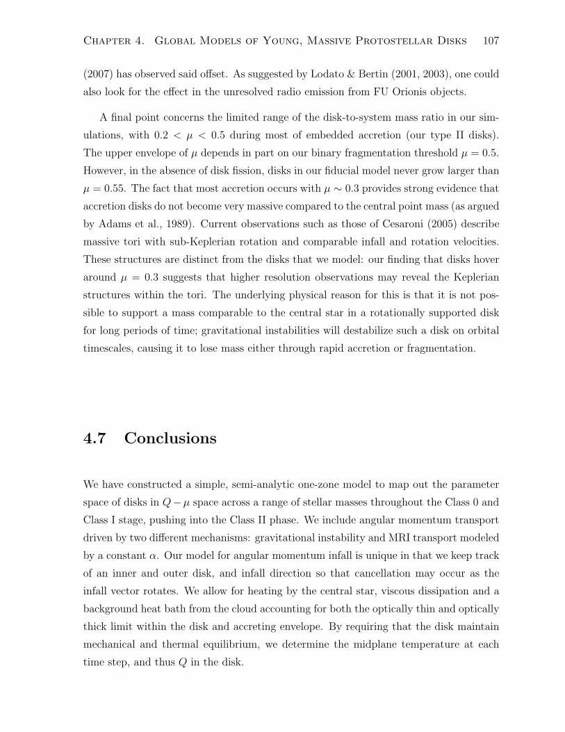
Chapter 4. Global Models of Young, Massive Protostellar Disks 107
(2007) has observed said o!set. As suggested by Lodato & Bertin (2001, 2003), one could
also look for the e!ect in the unresolved radio emission from FU Orionis objects.
A final point concerns the limited range of the disk-to-system mass ratio in our sim-
ulations, with 0.2 < µ < 0.5 during most of embedded accretion (our type II disks).
The upper envelope of µ depends in part on our binary fragmentation threshold µ = 0.5.
However, in the absence of disk fission, disks in our fiducial model never grow larger than
µ = 0.55. The fact that most accretion occurs with µ $ 0.3 provides strong evidence that
accretion disks do not become very massive compared to the central point mass (as argued
by Adams et al., 1989). Current observations such as those of Cesaroni (2005) describe
massive tori with sub-Keplerian rotation and comparable infall and rotation velocities.
These structures are distinct from the disks that we model: our finding that disks hover
around µ = 0.3 suggests that higher resolution observations may reveal the Keplerian
structures within the tori. The underlying physical reason for this is that it is not pos-
sible to support a mass comparable to the central star in a rotationally supported disk
for long periods of time; gravitational instabilities will destabilize such a disk on orbital
timescales, causing it to lose mass either through rapid accretion or fragmentation.
4.7 Conclusions
We have constructed a simple, semi-analytic one-zone model to map out the parameter
space of disks in Q&µ space across a range of stellar masses throughout the Class 0 and
Class I stage, pushing into the Class II phase. We include angular momentum transport
driven by two di!erent mechanisms: gravitational instability and MRI transport modeled
by a constant (. Our model for angular momentum infall is unique in that we keep track
of an inner and outer disk, and infall direction so that cancellation may occur as the
infall vector rotates. We allow for heating by the central star, viscous dissipation and a
background heat bath from the cloud accounting for both the optically thin and optically
thick limit within the disk and accreting envelope. By requiring that the disk maintain
mechanical and thermal equilibrium, we determine the midplane temperature at each
time step, and thus Q in the disk.

Chapter 4. Global Models of Young, Massive Protostellar Disks 108
4.7.1 Caveats
In interpreting the results of our calculations, it is important to keep several caveats in
mind. Our model for fragmentation, though rooted in simulations, includes one important
assumption: no matter how violently unstable a disk becomes, it can always fragment,
return to a marginally stable state, and continue accreting. While the existence of stars
well into the mass regime of fragmentation makes this outcome seem likely, it has yet to be
demonstrated in simulations. Equally untested is the hypothesis that when fragmentation
is strong enough, i.e., when Min + c3s/G so that Q , 1 (Gammie, 2001), accretion
onto the central star will be choked o!. KM06 have argued that accretion is sharply
destabilized when its rate exceeds 1.7 ) 10!3 M" yr!1, due to a drop in the Rosseland
opacity, and that this may be related to the stellar upper mass limit.
In order to explore a wide parameter space, we do not carry out detailed hydrodynamic
calculations to determine the onset of instability, but instead use results from previous
simulations, and develop analytic formulae that describe behavior intermediate between
the regimes which they explore. Although our approach is very approximate, it can be
made increasingly more realistic as additional numerical simulations become available.
Due to our one-zone prescription, we cannot resolve spiral structure or measure the degree
of non-Keplerian motion. In addition, we do not follow the evolution of fragments, nor
their interaction with the disk. Although we allow for the formation of binaries, we do
not follow their evolution and accretion, which limits our ability to make predictions
about mass ratios and angular momentum transfer between the disk and the companion.
Our model for angular momentum infall is responsible for the largest uncertainty in our
conclusions because di!erent realizations of the turbulent velocity field can alter the disk
size at a given epoch by a factor of a few. Nevertheless, these variations are well within
the analytic expectations for range of angular momenta in cores (KM06). Moreover, our
approach aims only to predict characteristics of the outer accretion disk, and lacks the
resolution to track the radial profiles of the disk’s properties.
Lastly, recall that our models rely on the fundamental assumption (§ 4.3.1) that a
disk’s behavior can be separated into dynamical and thermal properties, and in particular
that its dynamics are governed primarily by its mass fraction µ and Toomre parameter
Q.
With these caveats in mind, we summarize our results for two di!erent regimes:
< 2M" and > 2M".

Chapter 4. Global Models of Young, Massive Protostellar Disks 109
4.7.2 The Low Mass Regime
Our fiducial models predict that low mass stars will have higher values of µ than typically
assumed during early phases of formation. However, they should remain stable against
fragmentation throughout their evolution, dominated by MRI, long wavelength gravita-
tional instability, and once again MRI through their evolution through the three types of
disks discussed in §4.5. During the main accretion phase, disks will have masses of order
30% of the system mass. Typical outer radii are of order 50 AU, with outer temperatures
of 40 K during the main accretion phase, dropping to $ 10 K at 2 Myr. The surface
density is 10 & 20 g cm!2 during the main accretion phase, dropping o! rapidly at late
times causing the disk to become optically thin to its own radiation. As accretion shuts
down, and disks grow due to conservation of angular momentum, two key e!ects must be
considered: truncation and heating by other stars. At distances of 1000 AU, very ten-
uous disks are prone to truncation by passing stars particularly in denser clusters where
average stellar densities are as high as 105 stars pc!3 (Hillenbrand & Hartmann, 1998).
Similarly, as the disk edge extends towards other, potentially more luminous stars, the
actual flux received will increase, heating the disk above the $ 10K temperature that we
routinely find (Adams et al., 2006).
For core column densities more typical of high-mass star forming regions, local insta-
bilities do set in, despite the stabilizing influence higher temperatures associated with
these regions (neglecting the e!ects of nearby stars). This implies that environment may
be important in understanding disk evolution.
In contrast to our previous work (Kratter & Matzner, 2006; Matzner & Levin, 2005),
we find fragmentation at smaller radii. This is primarily due to our modified model
for (GI, which predicts lower accretion rates and consequently more fragmentation then
previously assumed. We note that our results for low-mass systems (final mass $ 1M")
are rather sensitive to details of the model, such as the value of (MRI and the way it is
combined with (GI.
4.7.3 The High Mass Regime
For more massive stars, we find high values of µ $ 0.35 and an extended period of
local fragmentation as the accretion rates peak. Temperatures at the disk outer edge
at $ 200 AU approach 100K for systems > 15M" during accretion. surface densities
hover around 50 g cm!2 during the main accretion phase, although by 2 Myr, the disks

Chapter 4. Global Models of Young, Massive Protostellar Disks 110
become optically thin in the FIR, as expected. Binary formation occurs regularly for
cores of order 30M" and higher, though as discussed in §4.3.6 this is strongly dependent
on the cosmic variance of the angular momentum: cores as small as 20M" form binaries
in our model when there is excess angular momentum infall. Although fragments accrete
with the disk according to equation [4.25], more massive stars maintain a small mass in
fragments (10!1 & 10!2M") in the disk when we end our simulations, suggesting that
fragments may persist to form low mass companions, as predicted in KM06 and suggested
by the simulations of Krumholz et al. (2007b).
Unlike their low mass counterparts, the conclusions we draw for massive stars are
minimally e!ected by the environmental variables in our model. For the entire range of
temperatures, densities, and nearly all angular momentum realizations, the conclusions
listed above hold true.

Chapter 5
Numerical Models of Rapidly
Accreting Disks
A version of this chapter has been published in The Astrophysical Journal as “On the Role
of Disks in the Formation of Stellar Systems: A Numerical Parameter Study”, Kratter,
K. M., Matzner, C. D., Krumholz, M. R., and Klein, R. I., vol. 708, pp1585-1597, 2010.
Reproduced by permission of the AAS.
5.1 Introduction
We have surveyed the role of disks in the formation of stellar systems analytically, but
our results are ultimately dependent on our model of gravitational instability driven
accretion. Although semi-analytical and low-dimensional studies can illuminate trends
and provide useful approximate results, disk fragmentation is inherently a nonlinear and
multidimensional process. For this reason we have embarked on a survey of idealized,
three-dimensional, numerical experiments to examine the role of GI as the mediator of
the accretion rate in self-gravitating disks, and as a mechanism for creating disk-born
companions.
We focus on the dynamics of disks around young, rapidly accretings protostars, for
which self-gravity is the key ingredient (Lin & Pringle, 1987; Gammie, 2001; Kratter
et al., 2008). GI plays a strong role in AGN disks as well, and possibly in other contexts
where disks are cold and accretion is fast.
We emphasize that these are numerical experiments, not simulations of star formation.
Our goal in conducting experiments is to isolate the important physical process, GI,
111

Chapter 5. Numerical Models 112
which dictates angular momentum transport and fragmentation. To do so, we separate
the dynamical problem from the thermal one. We exclude thermal physics from our
simulations entirely, while scanning a thermal parameter in our survey.
By this means we reduce the physical problem to two dimensionless parameters: one
for the disk’s temperature, another for its rotation period – both in units determined by its
mass accretion rate. We hold these fixed in each simulation by choosing well-controlled
initial conditions corresponding to self-similar core collapse. This parameterization is
a central aspect of our work: it forms the basis for our numerical survey; it allows
us to treat astrophysically relevant disks, including fragmentation and the formation
of binary companions, while also maintaining generality; and it distinguishes our work
from previous numerical studies of core collapse, disk formation, GI, and fragmentation.
We demonstrate that idealized disks like those presented here can capture many of the
important features of simulations with more complicated physics, with significantly lower
computational cost.
In this chapter we focus on the broad conclusions we can draw from our parameter
space study. We begin here by introducing our dimensionless parameters in §5.2. We
describe the initial conditions and the numerical code used in §5.3. In §5.4 we derive
analytic predictions for the behavior of disks as a function of our parameters. We describe
the main results from our numerical experiments in §5.5, with more detailed analysis in
§5.7. We compare them to other numerical and analytic models of star formation in §5.8.
5.2 A New Parameter Space for Studying Accretion
We consider the gravitational collapse of a rotating, quasi-spherical gas core onto a central
pointlike object, mediated by a disk. In the idealized picture we will explore in this
chapter, the disk and the mass flows into and out of it can be characterized by a few
simple parameters. At any given time, the central point mass (or masses, in cases where
fragmentation occurs) has mass M#, the disk has mass Md, and the combined mass of the
two is M#d. The disk is characterized by a constant sound speed cs,d. Material from the
core falls onto the disk with a mass accretion rate Min, and this material carries mean
specific angular momentum "j#in, and as a result it circularizes and goes into Keplerian
rotation at some radius Rk,in; the angular velocity of the orbit is %k,in.
Note that Min, jin, Rk,in and %k,in characterize the material that is just reaching the
disk at a given instant, and as a result they can vary with time – indeed, we will set up

Chapter 5. Numerical Models 113
our initial conditions to guarantee that they do vary with time in precisely the manner
required to ensure that certain dimensionless numbers remain constant as gas accretes.
In general in what follows, we refer to quantities associated with the central object with
subscript *, quantities associated with the disk with a subscript d, quantities associated
with infall with subscript in. Angle brackets indicate mass-weighted averages over the
disk (with subscript d) or over infalling mass (with subscript in).
We characterize our numerical experiments using two dimensionless parameters which
are well-adapted to systems undergoing rapid accretion. Because the behavior of young
protostellar disks will be dominated by infall, modelling their behavior in terms of di-
mensionless accretion rates is a natural choice.
We encapsulate the complicated physics of heating and cooling through the thermal
parameter
" =MinG
c3s,d
, (5.1)
which relates the infall mass accretion rate Min to the characteristic sound speed cs,d
of the disk material. Our parameter " is also related to the physics of core collapse
leading to star formation. If the initial core is characterized by a signal speed ce",c then
Min $ c3e",c/G, implying " $ c3
e",c/c3s,d – although there can be large variations around
this value (Larson, 1972; Foster & Chevalier, 1993). The second, rotational parameter
" =Min
M#d%k,in=
Min "j#3inG2M3
#d, (5.2)
compares the system’s accretion timescale, M#d/Min to the orbital timscale of infalling
gas. For the initial conditions we use in this work, the quantities "j#in and M#d evolve
in time while Min remains constant. They can be evaluated as functions of time, or
the current radius from which material is falling onto the system. To hold " fixed, we
specify a core rotation profile such that "j#in % M#d. Unlike ", " is independent of disk
heating and cooling, depending only on the core structure and velocity field. In general,
" compares the relative strength of rotation and gravity in the core. Systems with a large
value of " (e.g. accretion-induced collapse of a white dwarf) gain a significant amount of
mass in each orbit, and tend to be surrounded by thick, massive accretion disks, while
those with very low " (e.g. AGN) grow over many disk lifetimes, and tend to harbor thin
disks with little mass relative to the central object. We consider characteristic values
for our parameters in §5.2.1, and their evolution in the isothermal collapse of a rigidly
rotating Bonnor-Ebert sphere in §5.8.1.

Chapter 5. Numerical Models 114
The parameters " and " are more flexible than other dimensionless parameters used
to characterize collapsing cores like (therm = Etherm/Egrav and &rot = Erot/Egrav (Boden-
heimer et al., 1980; Miyama et al., 1984). While the latter rely implicitly on a quasi-static
core model, " and " can be evaluated for arbitrary infall models, and therefore for a wider
range astrophysical disk scenarios. Whereas (therm and &rot are zero dimensional descrip-
tions of the collapse problem, " and " can be functions of mass and hence describe time
(or scale) evolution.
In order to model disk behavior in terms of these two parameters, we hold " and "
fixed for each experiment via the self-similar collapse of a rotating, isothermal sphere
(§5.3.2). This strategy allows us to map directly between the input parameters, and
relevant properties of the system. Specifically, we expect dimensionless properties like
the disk-to-star mass ratio, Toomre parameter, Q = cs%/(.G$) (Toomre, 1964), stellar
multiplicity, etc., to fluctuate around well-defined mean values (see §5.3.4).
We aim to use our parameters " and " to: (a) explore the parameter space relevant
to a range of star formation scenarios; (b) better understand the disk parameters, both
locally and globally, which dictate the disk accretion rate and fragmentation properties;
(c) make predictions for disk behavior based on larger scale, observable quantities; and
(d) allow the results of more complicated and computationally expensive simulations to
be extended into other regimes.
5.2.1 Characteristic values of the accretion parameters
We base our estimates of " and " on observations of core rotation in low-mass and
massive star-forming regions (Myers & Fuller, 1992; Goodman et al., 1993; Williams &
Myers, 1999), as well as the analytical estimates of core rotation and disk temperature in
Matzner & Levin (2005), Krumholz (2006), KM06, and KMK08. Using simple models of
core collapse in which angular momentum is conserved in the collapse process and part
of the matter is cast away by protostellar outflows (Matzner & McKee, 2000), we find
that both " and " are higher in massive star formation than in low-mass star formation.
In our models, the characteristic value of " rises from $ 0.001 & 0.03 as one considers
increasingly massive cores for which turbulence is a larger fraction of the initial support.
The value of " is more complicated, as it reflects the disk’s thermal state as well as
infalling accretion rate, but the models of KMK08 and Krumholz (2006) indicate that its
characteristic value increases from < 1 to $ 10 as one considers higher and higher mass

Chapter 5. Numerical Models 115
cores – although the specific epoch in the core’s accretion history is also important. In the
case of massive stars, such rapid accretion has been observed as in Beltran et al. (2006)
and Barnes et al. (2008). Numerical simulations also find rapid accretion rates from cores
to disks. Simulations such as those of Banerjee & Pudritz (2007) report " $ 10 at early
times in both magnetized and non-magnetized models. We note that " has significant
fluctuations from core to core when turbulence is the source of rotation, and both " and "
are a!ected by variations of the core accretion rate around its characteristic value (Foster
& Chevalier, 1993).
A major goal of this work is to probe the evolution of disks with " / 1, as mass accre-
tion at this rate cannot be accommodated by the Shakura & Sunyaev (1973) model with
( < 1. Values of ( exceeding unity imply very strong GI, and possibly fragmentation.
5.3 Numerical Methodology
5.3.1 Numerical Code
We use the code ORION (Truelove et al., 1998; Klein, 1999; Fisher, 2002) to conduct
our numerical experiments . ORION is a parallel adaptive mesh refinement (AMR),
multi-fluid, radiation-hydrodynamics code with self-gravity and lagrangian sink parti-
cles (Krumholz et al. 2004). Radiation transport and multi-fluids are not used in the
present study. The gravito-hydrodynamic equations are solved using a conservative,
Godunov scheme, which is second order accurate in both space and time. The gravito-
hydrodynamic equations are:
+
+t' = &1 · ('v)&
9
i
MiW (x& xi) (5.3)
+
+t('v) = &1 · ('vv)&1P & '1$ (5.4)
&9
i
piW (x& xi)
+
+t('e) = &1 · [('e + P )v] + 'v ·1$ (5.5)
&9
i
EiW (x& xi)
Equations (5.3)-(5.6) are the equations of mass, momentum and energy conservation
respectively. In the equations above, Mi, pi, and Ei describe the rate at which mass and

Chapter 5. Numerical Models 116
momentum are transfered from the gas onto the ith lagrangian sink particles. Summa-
tions in these equations are over all sink particles present in the calculation. W (x) is a
weighting function that defines the spatial region over which the particles interact with
gas. The corresponding evolution equations for sink particles are
d
dtM = Mi (5.6)
d
dtxi =
pi
Mi(5.7)
d
dtpi = &Mi1$ + pi. (5.8)
These equations describe the motion of the point particles under the influence of gravity
while accreting mass and momentum from the surrounding gas.
The Poisson equation is solved by multilevel elliptic solvers via the multigrid method.
The potential $ is given by the Poisson equation
12$ = 4.G
#
' +9
i
Mi*(x& xi)
$
, (5.9)
and the gas pressure P is given by
P ='kBTg
µp= (0 & 1)'
'e& 1
2v2
(, (5.10)
where Tg is the gas temperature, µp is the mean particle mass, and 0 is the ratio of
specific heats in the gas. We adopt µp = 2.33mH, which is appropriate for standard
cosmic abundances of a gas of molecular hydrogen and helium.
We use the sink particle implementation described in Krumholz et al. (2004) to replace
cells which become too dense to resolve. Sink particle creation and AMR grid refinement
are based on the Truelove criterion (Truelove et al., 1997) which defines the maximum
density that can be well resolved in a grid code as:
' <' j =N2
J.c2s
G('xl)2, (5.11)
where, NJ is the Jeans number, here set to 0.125 for refinement, and 0.25 for sink creation,
and 'xl is the cell size on level l. When a cell violates the Jeans criterion, the local
region is refined to the next highest grid level. If the violation occurs on the maximum
level specified in the simulation, a sink particle is formed. Setting NJ to 0.125 is also
consistent with the resolution criterion in Nelson (2006). Sink particles within 4 cells

Chapter 5. Numerical Models 117
of each other are merged in order to suppress unphysical n-body interactions due to
limited resolution. At low resolution, unphysical sink particle formation and merging
can cause rapid advection of sink particles inwards onto the central star, generating
spurious accretion. Moreover, because an isothermal, rotating gas filament will collapse
infinitely to a line (Truelove et al., 1997; Inutsuka & Miyama, 1992), an entire spiral arm
can fragment and be merged into a single sink particle. To alleviate this problem, we
implement a small barotropic switch in the gas equation of state such that
0 = 1.0001, ' < 'Js/4 (5.12)
0 = 1.28, 'Js/4 < ' < 'Js , (5.13)
where the Js subscript indicates the Jean’s criterion used for sink formation. With
this prescription, gas is almost exactly isothermal until fragmentation is imminent, at
which point it sti!ens somewhat. This modest sti!ening helps turn linear filaments into
resolved spheres just prior to collapse and provides separation between newborn sink
particles. The primary e!ect of this sti!ening is to increase the resolution of the most
unstable wavelength in a given simulation, at the expense of some dynamical range. We
describe the influence of this sti!ening on our results in §5.7.1, where we conduct some
experiments in which it is turned o!.
As described via equations (5.3)-(5.6), sink particles both accrete from and interact
with the gas and each other via gravity. Accretion rates are computed using a modified
Bondi-Hoyle formula which prevents gas which is not gravitationally bound to the par-
ticles from accreting. See Krumholz et al. (2004) and O!ner et al. (2008) for a detailed
study of the e!ects of sink particle parameters. Note that we also use a secondary, spa-
tial criterion for AMR refinement based on an analytic prediction for the disk size as a
function of time (see §5.3.3).
5.3.2 Initial conditions
We initialize each run with an isothermal sphere:
'(r) =Ac2
s,core
4.Gr2. (5.14)
There is a small amount of rotational motion in our initial conditions, but no radial
motion. A core with this profile is out of virial balance when A > 2, and accretes at a

Chapter 5. Numerical Models 118
rate
M =c3s,core
G)
/1
20.975, (A = 2)
(2A)3/2/.. (A+ 2)(5.15)
The value for A = 2 represents the Shu (1977b) inside-out collapse solution, whereas the
limit A + 2 is derived assuming pressureless collapse of each mass shell. It is possible
to predict M analytically (Shu, 1977b), but in practice we initialize our simulations with
a range of values A > 2 and measure M just outside the disk. Because our equation
of state is isothermal up to densities well above the typical disk density (cs,d = cs,core),
MG/c3s,core is equivalent to our parameter ".
In order to set the value of our rotational parameter " and hold it fixed, we initialize
our cores with a constant, subsonic rotational velocity:
vrot = 5% = 2Acs
%"
"
&1/3
, (5.16)
where 5 is the cylindrical radius. We arbitrarily choose a constant velocity rather than
rigid rotation on spheres in order to concentrate accretion near the outer disk radii. Our
definition of " in terms of the mean value of jin rather than its maximum value is intended
to reduce the sensitivity of our results to the choice of rotational profile.
Given these initial conditions, our parameters " and " remain constant throughout
the simulation, while the collapsed mass and disk radius (as determined by the Keplerian
circularization radius of the infalling material) increase linearly with time. We define a
resolution parameter,
# =Rk,in
dxmin, (5.17)
to quantify the influence of numerics on our results. Because we hold the minimum grid
spacing dxmin constant, # increases % t as the simulation progresses.
By artificially controlling the infall parameters of our disks, and then watching them
evolve in resolution, we gain insight into the physical behavior of accretion with certain
values of " and ", as captured in a numerical simulation with a given dynamical range
(#). Our initial conditions are necessarily ideal, allowing us to perform controlled exper-
iments. That we use a “core model” at all is purely for numerical convenience. Realistic
star-forming cores will undoubtedly look very di!erent with turbulence, and time vary-
ing accretion of mass and angular momentum, but before addressing more complicated
scenarios we must establish the predictive value of our parameters.

Chapter 5. Numerical Models 119
5.3.3 Domain and Resolution
Due to the dimensionless nature of these experiments, we do not use physical units to
analyze our runs. The base computational grid is 1283 cells, and for standard runs we
use nine levels of refinement, with a factor of two increase in resolution per level: this
gives an e!ective resolution of 65, 5363. More relevant to our results, however, is the
resolution with which our disks are resolved: # <$ 102. To compare this to relevant scales
in star formation, this is equivalent to sub-AU resolution in disks of $ 50& 100 AU.
The initial core has a diameter equal to one half of the full grid on the base level. The
gravity solver obeys periodic boundary conditions on the largest scale; as the disk is 2.5
to 3 orders of magnitude smaller than the grid boundaries, disk dynamics are una!ected
by this choice. The initial radius of the current infall is (.")!2/3Rk,in (from equations
(5.2), (5.14), and (5.15)); although this is much larger than the disk itself, it is still
$ 15& 40 times smaller than the initial core and $ 30& 80 times smaller than the base
grid. Tidal distortions of the infall are therefore very small, although they may be the
dominant seeds for the GI. We return to this issue in §5.7.3, where we compare two runs
in which only the tidal e!ects should be di!erent.
In addition to the density criterion for grid refinement described in §5.3, we also refine
spatially to ensure that the entire disk is resolved at the highest grid level. We use " and
" to predict the outer disk radius (see §5.4), and refine to the highest resolution within 1.5
times this radius horizontally, and within 0.4 times this radius vertically. We find that we
accurately capture the vertical and radial extent of the disk with this prescription, and
the density criterion ensures that any matter at disk-densities extending beyond these
radii will automatically be refined.
5.3.4 Dynamical Self-Similarity
Because our goal is to conduct a parameter study isolating the e!ects of our parameters
" and ", we hold each fixed during a single run. At a given resolution #, we expect
the simulation to produce consistent results regarding the behavior of the accretion disk,
the role of GI, and the fragmentation of our idealized disks into binary or multiple
stars. Since # increases linearly in time, each simulation serves as a resolution study in
which numerical e!ects diminish in importance as the run progresses. Because GI is an
intrinsically unsteady phenomenon, a disk should fluctuate around its mean values even
when all three of ", ", and # are fixed. Because of this, and because # changes over the

Chapter 5. Numerical Models 120
Figure 5.1: Two examples of single, binary, and multiple systems. The resolution across
each panel is 328x328 grid cells. The single runs are " = 2.9, " =0 .018 (top), " =
1.6, " = 0.009 (bottom). The binaries are " = 4.2, " = 0.014 (top), " = 23.4, " = 0.008,
(bottom). The multiples are " = 3.0, " =0 .016 (top), " = 2.4, " = 0.01 (bottom). Black
circles with plus signs indicate the locations of sink particles. These correspond to runs
5, 1, 9, 16, 7, and 4 respectively.
run, we expect our runs to be self-similar, but only in a limited, statistical sense.
Moreover, whereas many physical systems are captured perfectly in the limit of infinite
resolution (# *2), this is not true of isothermal, gravitational gas dynamics, in which
the minimum mass and spacing of fragments both scale as #!1 (Inutsuka & Miyama,
1992). For this reason we quote the resolution # whenever reporting on the state of the
disk-star system.
We note that there exists a minimum scale in real accretion disks as well, namely
the opacity-limited minimum fragment mass (Rees, 1976). The finite dynamical range of
our numerical simulations is therefore analogous to a phenomenon of Nature, albeit for
entirely di!erent reasons.

Chapter 5. Numerical Models 121
5.4 Disk properties in terms of the accretion param-
eters
To assess the physical importance of " and ", it is useful to consider the case of a
single star and its accretion disk. Because many ", " pairs lead to fragmentation, this
assumption is only self-consistent within a subregion of our parameter space; nevertheless
it helps to guide our interpretation of the numerical results. In order to associate results
from our parameters with those of previous studies, we also derive expressions for disk
averaged quantities such as Q and the disk-to-system mass ratio, µ as a function of "
and ".
The combination %"
"
&1/3
="j#in cs,d
GM#d=
cs,d
vk,in(5.18)
is particularly useful, since it provides an estimate for the disk’s aspect ratio (the scale
height compared to the circularization radius). Being independent of M , it is more a
property of the disk than of the accretion flow.
The other important dimensionless quantity whose mean value depends primarily on
" and " (and slowly on resolution) is the disk-to-system mass ratio
µ =Md
M#d. (5.19)
When the disk is the sole repository of angular momentum, the specific angular mo-
mentum stored in the disk is related to the infalling angular momentum via:
jd =
%Jin
"j#in M#d
&"j#inµ
(5.20)
where Jin is the total angular momentum accreted, so that Jin/("j#in M#d) = 1/(lj +1) in
an accretion scenario where "j#in % Mlj#d. In our simulations lj = 1, so jd = "j#in /(2µ).
Given the relation between jd and "j#in, we can define
Rd
%d
=
=
[(lj + 1)µ]!2 Rk,in
[(lj + 1)µ]3 %k,in
(5.21)
which relate the disk’s characteristic quantities (not the location of its outer edge) to
conditions at the current circularization radius Rk,in = "j#2in /(GM#d). Such “charac-
teristic” quantities are valuable for describing properties of the disk as a whole, rather
than at single location, with an e!ective mass weighting. If we further suppose that

Chapter 5. Numerical Models 122
the disk’s column density varies with radius as $(r) % r!k! (we expect k! . 3/2
for a constant Q, isothermal disk), we may define its characteristic column density
$d = (1& k!/2)Md/(.R2d):
$d . f!G2M3
#d
"j#4inµ5 (5.22)
where f! = (1& k!/2)(1 + lj)4/.. Using equations (5.18) and (5.21)-(5.22), we can
rewrite the Toomre stability parameter Q (ignoring the di!erence between % and the
epicyclic frequency,), for simplicity):
Q =cs)
.G$* cs%d
.G$d(5.23)
Qd .f!1
Q
µ2
cs,d "j#inGM#d
=
%"
"
&1/3 f!1Q
µ2. (5.24)
where fQ = (1& k!/2)(1 + lj). To the extent that we expect Qd $ 1 in any disk with a
strong GI, this suggests µ $ ("/")1/6(1 & k!/2)!1/2(1 + lj)!1/2; and because we expect
that µ has an upper limit of around 0.5 (see §5.5 and discussion in KMK08 and Shu
et al., 1990), we see there is an upper limit to "/" above which the system is likely to
become binary or multiple. This is not surprising, as µ is proportional to scale height
when Q is constant; equation (5.24) simply accounts self-consistently for the fact that µ
also a!ects Rd.
To go any further with analytical arguments, we must introduce a Shakura & Sunyaev
(1973) ( viscosity parameterization, in which steady accretion occurs at a rate
M# =3(
Qd
c3s,d
G(5.25)
Using the definition of "
" . 3(
Qd
1
1& µ(5.26)
Insofar as Q $ 1 when the GI is active, the e!ective value of ( induced by a strong GI
is directly proportional to ". We have made the simplifying assumption that accretion
through the disk is roughly constant, although the factor of (1 & µ) accounts for the
di!erence between the infall rate and the rate at which the disk processes material onto
the star.

Chapter 5. Numerical Models 123
The magnitude of " has important implications for disk evolution. As discussed
previously by KMK08, " (called 0in there) a!ects µ through the relation
µ
µ%k,in= "
%1
µ& 1
&
& M#
Md%k,in. (5.27)
. "
%1
µ& 1
&
& 3
%
1& k!
2
&
(1 + lj)(µ
%"
"
&2/3
,
where the second line uses disk-averaged quantities to construct a mean accretion rate
from equation (5.25). Our runs approach a statistical steady state, µ . 0 (although the
dimensional quantity Md continues to increase.) We expect µ to saturate at the value
for which the two terms on the right of equation (5.27) are equal,
µ* (B2 + 2B)1/2 &B, where B ="1/3"2/3
3(2& k!)(1 + lj)(. (5.28)
Here B is the linear coe#cient for the quadratic in equation (5.27). The disk mass
fraction µ increases with B, so both " and " have a positive e!ect on µ, whereas ( tends
to suppress the disk mass.
The scaling of disk properties with " is in accord with intuitive expectations. An
increase in " corresponds to an increase in accretion rate at fixed disk sound speed, and
as a result the equilibrium disk mass rises. Similarly, an increase in ( corresponds to an
increase in the rate at which the disk can transport angular momentum and mass at a
fixed rate of mass and angular momentum inflow, allowing the disk to drain and reducing
its relative mass.
Less intuitive, however, is the fact that equations (5.24) and (5.28) predict that rota-
tion has a stabilizing e!ect on massive disk systems, in the sense that Qd increases with
" so long as µ > 0. This can be seen by noting that d ln µ/d ln B = (1&µ)/(2&µ). Note
that, when B is small and µ .3
2B, equation (5.23) implies Qd . 3(/" in accordance
with equation (5.25). Thus for small values of µ, we recover the dependence of Q solely on
", in accord with Gammie (2001). As µ grows and saturates, " becomes more important
in setting Q. We discuss the stabilizing influence of " in §5.5.3.
Because the e!ective value of ( induced by the GI is a function of disk parameters,
we cannot say more without invoking a model for ((", ") or ((Q, µ) as in KMK08. We
use the above relations to guide our interpretation of our simulation results, specifically
the dependence of disk parameters like µ, Qd, (, and the fragmentation boundary, on "
and ".

Chapter 5. Numerical Models 124
5.5 Results
Each of our runs produces either a disk surrounding a single star, or binary or multiple
star system formed via disk fragmentation; Figure 5.1 depicts examples of each outcome.
We use these three possible morphologies to organize our description of the experiments.
We explore the properties of each type of disk below as well as examine the conditions
at the time of fragmentation.
The division between single and fragmenting disks in " and " is relatively clear from
our results, as shown in Figure 5.2. Several trends are easily identified. First, there is a
critical " beyond which disks fragment independent of the value of ". Below this critical
" value, there is a weak stabilizing e!ect of increasing ". As " increases, disks transition
from singles in to multiples, and finally into binaries. We discuss the distinction between
binaries and multiples in §5.6. This stabilizing e!ect of " is predicted by equation (5.23),
although it is somewhat counter intuitive. We discuss in §5.5.3 that the stabilization is
often masked thermal e!ects in real collapsing systems.
In table 5.1 we list properties of the final state for all of our runs, their final multiplicity
(S, B, or M for single, binary, or multiple, respectively), and the disk-to-star(s) mass ratio
µf measured at the time at which we stop each experiment, as well as the maximum
resolution #n. Note that the disk extends somewhat beyond Rk,in: therefore the disk as
a whole is somewhat better resolved than the value of #n would suggest. For the disks
which fragment, we also list the value of µf , #f and Q just before fragmentation occurs.
In table 5.2 we describe those disks which do not fragment: we list the analytic
estimate for the characteristic value Toomre’s Q, Qd, the measured minimum of Q2D
(equation 5.29), the radial power law k! which characterizes $(r) for a range of radii
extending from the accretion zone of the inner sink particle to the circularization radius
Rk,in, the final disk resolution, #n, and the characteristic disk radius, Rd (equation (5.21).
5.5.1 The Fragmentation Boundary and Q
It is di#cult to measure a single value of Q to characterize a disk strongly perturbed
by GI, so we consider two estimates: a two dimensional measurement Q2D, and a one-
dimensional measure Qav(r) based on azimuthally-averaged quantities.
Q2D(r,$) =cs)
.G$, (5.29)

Chapter 5. Numerical Models 125
# " 102" N# µf #f Q2D µ #n
1 1.6 0.9 S ... ... ... 0.49 99
2 1.9 0.8 S ... ... ... 0.40 88
3 2.2 2.5 S ... ... ... 0.56 82
4 2.4 1.0 M 0.43 77 0.69 0.16 98
5 2.9 1.8 S ... ... ... 0.53 86
6 2.9 0.8 M 0.40 51 0.72 0.14 78
7 3.0 0.4 M 0.33 50 0.48 0.11 77
8 3.4 0.7 M 0.40 66 0.37 0.16 70
9 4.2 1.4 B 0.51 56 0.19 0.33 72
10 4.6 2.1 M 0.54 71 0.42 0.23 123
11 4.6 0.7 B 0.35 28 0.52 0.12 52
12 4.9 0.9 B 0.37 26 0.74 0.19 59
13 5.4 0.4 B 0.38 38 0.33 0.19 64
14 5.4 0.7 B 0.31 49 0.85 0.21 62
15 5.4 7.5 B 0.72 99 0.20 0.59 129
16* 23.4 0.8 B 0.25 5 0.83 0.10 84
17* 24.9 0.4 B 0.15 3 0.59 0.11 61
18* 41.2 0.8 B 0.13 5 1.33 0.10 58
Table 5.1: Each run is labelled by ", ", multiplicity outcome, the final value of the disk-
to-star(s) mass ratio,µ and the final resolution, #n. Values of " are quoted in units
of 10!2. For fragmenting runs the disk resolution #f , Q2D (equation 5.29) and µf at
the time of fragmentation are listed as well. S runs are single objects with no physical
fragmentation. B’s are binaries which form two distinct objects each with a disk, and
M are those with three or more stars which survive for many orbits. * indicates runs
which are not su#ciently well resolved at the time of fragmentation to make meaningful
measures of µf , and Q.
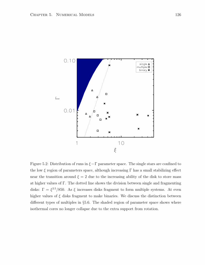
Chapter 5. Numerical Models 126
Figure 5.2: Distribution of runs in "&" parameter space. The single stars are confined to
the low " region of parameters space, although increasing " has a small stabilizing e!ect
near the transition around " = 2 due to the increasing ability of the disk to store mass
at higher values of ". The dotted line shows the division between single and fragmenting
disks: " = "2.5/850. As " increases disks fragment to form multiple systems. At even
higher values of " disks fragment to make binaries. We discuss the distinction between
di!erent types of multiples in §5.6. The shaded region of parameter space shows where
isothermal cores no longer collapse due to the extra support from rotation.

Chapter 5. Numerical Models 127
# " 102" µ Qd Q2D k! #n Rd
1 1.6 0.9 0.49 1.6 0.96 1.5 99 103
2 1.9 0.8 0.40 1.5 1.10 1.3 88 138
3 2.2 2.5 0.56 3.7 0.83 1.8 82 65
5 2.9 1.8 0.53 2.2 0.56 1.7 86 77
Table 5.2: Non-fragmenting runs (numbers as from table 5.1). We list values for the
characteristic predicted value of Toomre’s Q, Qd (equation 5.23), as well as the measured
disk minimum, Q2D equation (5.29). We also list the slope of the surface density profile,
k! averaged over several disk orbits, the final resolutions, and Rd at the end of the run
(equation 5.21)
Qav(r) =cs(r))(r)
.G$(r)(5.30)
where bars represent azimuthal averages, and ) is calculated directly from the gravita-
tional potential of the disk+stars. As Figure 5.3 shows, the two-dimensional estimate
shows a great deal of structure which is not captured by the azimuthal average, let alone
by Qd. Moreover, while the minimum of the averaged quantity is close to two, the two
dimensional quantity drops to Q $ 0.3. We find that the best predictor of fragmentation
is the minimum of a smoothed version of the two-dimensional quantity (smoothed over
a local Jeans length to exclude meaningless fluctuations), although Qd shows a similar
trend. We use this smoothed minimum quantity in table 5.1, and compare it to the
analytic estimate Qd in table 5.2 for non-fragmenting disks.
The critical values of Q at which fragmentation sets in depend on the exact method
used for calculation (e.g. Qav or Q2D). The canonical Q = 1 boundary only indicates
the instability of axisymmetric perturbations in razor-thin disks (Toomre, 1964). As
discussed by numerous authors, the fragmentation criterion is somewhat di!erent for
thick disks (Goldreich & Lynden-Bell, 1965; Laughlin et al., 1997a, 1998), and for the
growth of higher order azimuthal modes (Adams et al., 1989; Shu et al., 1990; Laughlin
& Korchagin, 1996b).
Because our disks are thick, the fragmentation boundary cannot be drawn in Q-
space alone. We use Q2D and µ in Figure 5.4 to demarcate the fragmentation boundary.
Labeled curves illustrate that the critical Q for fragmentation depends on the disk scale
height (equation 5.18). At a given value of Q, a disk with a larger value of µ will have a
larger aspect ratio, and will therefore be more stable. Recall from equation (5.18), that

Chapter 5. Numerical Models 128
Figure 5.3: Top: Qav in a disk with " = 2.9, " = 0.018. The current disk radius,
Rk,in is shown as well. Bottom: Log(Q2D) (equation 5.29) in the same disk. While the
azimuthally averaged quantity changes only moderately over the extent of the disk, the
full two-dimensional quantity varies widely at a given radius. Q is calculated using )
derived from the gravitational potential, which generates the artifacts observed at the
edges of the disk. Here and in all figures, we use *x to signify the resolution.

Chapter 5. Numerical Models 129
the disk aspect ratio is proportional to ("/")1/3.
This trend is consistent with the results of Goldreich & Lynden-Bell (1965) for thick
disks; because the column of material is spread out over a larger distance, H, its self-
gravity is somewhat diluted. The fact that two parameters are necessary to describe
fragmentation is also apparent in Figure 5.2, where the boundary between single and
multiple systems is a diagonal line through the parameter space.
Although two criteria are necessary to prescribe the fragmentation boundary, we ob-
serve a direct correspondence between µ and ", and " and Toomre’s Q. Figure 5.5 shows
that µ ( 2"1/3 for both single star disks, and just prior to the onset of fragmentation
in disks that form binaries and multiples. We find a similar correspondence between "
and the combination Qdµ, which is a direct correlation between " and Q defined with
respect to the disk circularization radius (using Rd in the definition of Qd brings in an
extra factor of µ.)
5.5.2 Properties of non-fragmenting disks
Although we quote a single power law value for the surface density profiles of disks in
table 5.2, the surface density structure is somewhat more complex. We find that the
disks show some evidence of a broken power law structure: an inner region, characterized
by k!, where disk material is being accreted inwards, and an outer region characterized
by a steep, variable power law due to the outward spread of low-density, high angular
momentum material. We find disks characterized by slopes between k! = 1 & 2. Clus-
tering around k! = 3/2 is expected, as this is the steady-state slope for a constant Q,
isothermal disk. Our measurements of Q(r) (equation 5.29) show fluctuating, but roughly
constant value over the disk radius. Note that the slope of the inner disk region tends
to increase with ". Figure 5.6 shows normalized radial profiles for the non-fragmenting
disks. Profiles are averaged over approximately three disk orbital periods. The flattening
at small radii is due to the increasing numerical viscosity in this region (§5.7.3).
We find an upper mass limit of µ $ 0.55, for single stars, which means that disks do
not grow more massive than their central star. A maximum disk mass has been predicted
by Shu et al. (1990) as a consequence of the SLING mechanism. Such an upper limit is
expected as eccentric gravitational instabilities in massive disks shift the center of mass
of the system away from the central object. Indeed, we observe this wobble in binary
forming runs. The subsequent orbital motion of the primary object acts as an indirect

Chapter 5. Numerical Models 130
Figure 5.4: Steady-state and pre-fragmentation values of Q and µ for single stars and
fragmenting disks respectively. We use the minimum of Q2D as described in §5.5.1. Sym-
bols indicate the morphological outcome. Note that the non-fragmenting disks (large
triangles) have the highest value of µ for a given Q. Contours show the predicted scale-
height as a function of Q and µ. It is clear that the single disks lie at systematically
higher scale heights. We have assumed k! = 3/2 in calculating scaleheight contours as a
function of Q and µ.

Chapter 5. Numerical Models 131
Figure 5.5: At right " vs µ with the fit in equation (5.31) overplotted. At left, Qdµ vs "
with the scaling Q % "!1/3 overplotted. Runs, 16, 17, 18 are omitted as the low resolution
at the time of fragmentation makes measurements of µ and therefore Qd unreliable.
potential exciting strong m = 1 mode perturbations which can induce binary formation
(Shu et al., 1990). We find that this maximum value is consistent with their prediction.
Using the analytic expressions above, we can also derive an expression for an e!ective
Shakura-Sunyaev (. In this regime of parameter space, " and " are always such that
B , 1 (assuming ( does not stray far from unity). We therefore expect that µ %"1/6"1/3(!1/2. Using this relation we can find a functional form of ((", "). Our fit to the
data shown in Figure 5.5 implies
µ ( 2"1/3, (5.31)
with some scatter for both single disks and fragmenting disks just prior to fragmentation.
We can use this fit to infer a scaling relation for ( using equation (5.28) in the limit
µ $3
2B:
(d (1
18(2& k!)2(1 + lj)2
"2/3
"1/3. (5.32)
The scaling is consistent with our expectation that driving the disk with a higher "
causes it to process materially more rapidly, while increasing " decreases the e#ciency
with which the disk accretes. Equation (5.32) predicts disk averaged values of ( for single
star disks between $ 0.3& 0.8. These values are consistent with the observed accretion
rates, and numerically calculated torques (§5.5.4).

Chapter 5. Numerical Models 132
Figure 5.6: Normalized density profiles for the single-star disks. Profiles are azimuthal
averages of surface densities over the final $ 3 disk orbital periods. We find that while
the inner regions are reasonably approximated by power law slopes, the slope steepens
towards the disk edge. For comparison, slopes of k! = 1, 1.5, and 2 are plotted as well.
Runs are labelled according to their values in table 5.1.

Chapter 5. Numerical Models 133
Figure 5.7: Azimuthal averages of di!erent components of torque expressed as an e!ective
( (equation 5.34) for run #8. The straight line, (d (equation 5.32) is plotted for com-
parison. The agreement between the analytic value of (d and the combined contribution
from the other components is best near the expected disk radius Rk,in.
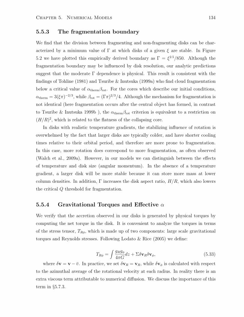
Chapter 5. Numerical Models 134
5.5.3 The fragmentation boundary
We find that the division between fragmenting and non-fragmenting disks can be char-
acterized by a minimum value of " at which disks of a given " are stable. In Figure
5.2 we have plotted this empirically derived boundary as " = "2.5/850. Although the
fragmentation boundary may be influenced by disk resolution, our analytic predictions
suggest that the moderate " dependence is physical. This result is consistent with the
findings of Tohline (1981) and Tsuribe & Inutsuka (1999a) who find cloud fragmentation
below a critical value of (therm&rot. For the cores which describe our initial conditions,
(therm = 3(".)!2/3, while &rot = (".)2/3/4. Although the mechanism for fragmentation is
not identical (here fragmentation occurs after the central object has formed, in contrast
to Tsuribe & Inutsuka 1999b ), the (therm&rot criterion is equivalent to a restriction on
(H/R)2, which is related to the flatness of the collapsing core.
In disks with realistic temperature gradients, the stabilizing influence of rotation is
overwhelmed by the fact that larger disks are typically colder, and have shorter cooling
times relative to their orbital period, and therefore are more prone to fragmentation.
In this case, more rotation does correspond to more fragmentation, as often observed
(Walch et al., 2009a). However, in our models we can distinguish between the e!ects
of temperature and disk size (angular momentum). In the absence of a temperature
gradient, a larger disk will be more stable because it can store more mass at lower
column densities. In addition, " increases the disk aspect ratio, H/R, which also lowers
the critical Q threshold for fragmentation.
5.5.4 Gravitational Torques and E!ective (
We verify that the accretion observed in our disks is generated by physical torques by
computing the net torque in the disk. It is convenient to analyze the torques in terms
of the stress tensor, TR!, which is made up of two components: large scale gravitational
torques and Reynolds stresses. Following Lodato & Rice (2005) we define:
TR! =* gRg!
4.Gdz + $*vR*v!, (5.33)
where *v = v& v. In practice, we set *vR = vR, while *v! is calculated with respect
to the azimuthal average of the rotational velocity at each radius. In reality there is an
extra viscous term attributable to numerical di!usion. We discuss the importance of this
term in §5.7.3.

Chapter 5. Numerical Models 135
The first term in equation (5.33) represents torques due to large scale density fluc-
tuations in spiral arms, while the second is due to Reynolds stresses from deviations
in the velocity field from a Keplerian (or at least radial) velocity profile. To facilitate
comparison with analytic models, the torques can be represented as an e!ective ( where:
TR! =
)))))dln%
dlnR
))))) ($c2s (5.34)
We can compare these torques to the characteristic disk (d in equation (5.32) at a
snapshot in time. Figure 5.7 compares (d to the azimuthal average of the physical torques
for one of our runs. We also show the expected contribution from numerical di!usion
(see §5.7.3). The accretion expected from these three components is consistent with the
time averaged total accretion rate onto the star. Due to the short term variability of
the accretion rate, the two do not match up exactly. It is interesting to note the radial
dependence of the Reynolds stress term, which in the inner region decays rapidly, before
rising again, due to the presence of spiral arms. In both the azimuthal average and the
two dimensional distribution we see that at small radii numerical di!usion dominates,
whereas at large radii deviations in the azimuthal velocity which generate Reynolds
stresses are spatially correlated with the spiral arms.
5.5.5 Vertical Structure
When the disks reach su#cient resolution, we can resolve the vertical motions and struc-
ture of the disk. We defer a detailed analysis of the vertical structures to a later paper,
but discuss several general trends here. Depending on the run parameters, the disk scale
height is ultimately resolved by 10-25 grid cells. We observe only moderate transonic
motions in the vertical direction of order M $ 1& 2. Figure 5.8 shows two slices of the
z-component of the velocity field for a single system, one through the X-Z plane, and the
other through the disk midplane. Although there is significant substructure, the motions
are mostly transonic.
We also observe a dichotomy in the vertical structure between single and binary disks.
Although the values of " and " should dictate the scaleheight (see equation (5.11)), and
therefore higher " disks which become binaries should have smaller scaleheights to begin
with, we observe a transition in scaleheight when a disk fragments and becomes a binary.
Large plumes seen in single disks, like those shown in Figure 5.11 contain relatively low
density, high angular momentum material being flung o! of the disk. The relatively sharp

Chapter 5. Numerical Models 136
Figure 5.8: Cuts along the vertical axis and disk midplane of the vertical velocity, nor-
malized to the disk sound speed. Clearly most of the vertical motions in the disk are
transonic, although at the edges of the disk the velocities exceed M $ 1.

Chapter 5. Numerical Models 137
outer edges are created by the accretion shock of infalling material onto these plumes.
We observe small scale circulation patterns which support these long lived structures.
Disks surrounding binaries, by comparison remain relatively thin; in particular while
the circumprimary disks are slightly pu#er than expected from pure thermal support,
the circumbinary disk (when present) is su#ciently thin that we do not consider it well
resolved. This implies that the e!ective " values that binary disks see declines more
than " according to equation (5.18). This is consistent with the statement that some of
the infalling angular momentum is transferred into the orbit instead of on to the disks
themselves.
5.5.6 Fourier Component Analysis
In order to characterize the accretion mechanism we compute the relative radially inte-
grated amplitudes of the low order azimuthal modes, or Cm. We map the disk column
density onto a polar grid and compute the amplitude in each fourier mode as:
Cm =
)))" 2*0
" rdrin
$(r,$)re!im!drd$)))
)))" 2*0
" rdrin
$(r,$)rdrd$)))
, (5.35)
or the absolute value of the strength in the mode normalized to the m = 0 mode. We
find that while the relative amplitudes change in time for a given run, and vary from
one run to another, the m = 1 and m = 2 modes are dominant. The power typically
decreases towards higher modes, though there is some variation. The presence of strong
odd-m modes is also apparent from the wobble of the central star. Binary formation
due to the saturation of an m = 1 mode was predicted by Adams et al. (1989) and
Shu et al. (1990). The SLING mechanism relies on forcing of m = 1 modes by the
indirect potential of the moving central mass. Waves are launched at the outer Lindblad
resonance, get refracted at the Q barrier surrounding corotation, propagate back out to
the outer Lindblad resonance, refract again at the Q barrier, propagate out towards the
disk edge, and get reflected back in (see figure 1 of Shu et al. 1990). While we see evidence
for this in some disks, we are unable to confirm that this is the dominant mechanism for
fragmentation in all of our disks.
To assess the e!ectiveness of the SLING mechanism we measured the orbital velocity
of the central star about the center of mass, prior to fragmentation. As seen in Fig. 5.9,
in run #14, we see clear growth of the orbital velocity (normalized to the sound speed)
up until fragmentation. This same pattern is not seen in all other fragmenting runs.

Chapter 5. Numerical Models 138
Figure 5.9: Top: the x and y components of the velocity of the central star normalized
by the disk sound speed for run #14. Bottom: the combined orbital velocity of the star
normalized to the sound speed. The velocity o!set grows until the disk fragments.

Chapter 5. Numerical Models 139
In addition, while Adams et al. (1989) predict an upper mass limit to disks due to the
SLING mechanism (of about 1/3 the central object mass) we find disk masses can grow
comparable to the central star. We expect that this di!erence in the mass at saturation
may be due to leakage of waves at the outer edge of the disks, as the SLING mechanism
relies on sharp disk outer boundaries to reflect the waves.
We find that prior to binary formation, the m = 1 mode often grows and becomes
dominant over m = 2, yet single star disks exist with more power in m = 1 than m = 2,
and disks fragment when the m = 2 is dominant. In some runs there are velocity o!set
spikes prior to fragmentation, but most exhibit the gradual growth seen in Fig. 5.9,
though the progression is less smooth.
We interpret this to be evidence that multiple modes may coexist and contribute
to fragmentation, as discussed by Laughlin & Korchagin (1996b). While we do not
observe the precise mode coupling that these authors describe, there appear to be some
correlations between the m = 1& 3 modes.
Figure 5.10 shows the mode power spectrum juxtaposed with the column density just
before binary formation for runs #13 and # 8, demonstrating the appearance of disks
with di!erent dominant fourier modes.
There has been much discussion in the literature on the relative strength of global
versus local modes dominating the accretion flow. Typically the assumption has been
that low order modes signify globally-dominated accretion, and high order modes locally-
dominated accretion (Balbus & Papaloizou, 1999; Laughlin et al., 1997b; Gammie, 2001;
Adams et al., 1989; Lodato & Rice, 2005; Kratter et al., 2008). This of course depends on
how tightly wound the spirals are. We can clearly observe that the structures in the disk
are “global” in that they extend over more than a scale height in radius. However, because
the modes do not appear to be long-lived, it is di#cult to measure their wavenumbers,
or the pitch angle of the spirals.
5.6 The formation of binaries and multiples
As shown by Figure 5.2, a large swath of our parameter space is characterized by bi-
nary and multiple formation. We find that the division between fragmenting and non-
fragmenting disks can be characterized by a minimum value of " at which disks of a given
" are stable. In Figure 5.2 we have plotted this boundary as " = "2.5/850.
While we do not claim that our numerical experiments are a true representation of the

Chapter 5. Numerical Models 140
Figure 5.10: Examples of the log of the disk surface density and corresponding fourier
mode strengths when an m = 2 mode dominates (top, run #13) and when an m = 1
mode dominates bottom (run #8), both within about one disk orbit of fragmentation.
At bottom one can clearly see both the overall asymmetry and the pronounced m = 2
spiral. Note that run #8 shows a similar growth pattern to Fig. 5.9, while the top image,
run #13 does not.

Chapter 5. Numerical Models 141
binary formation process, we do expect to find binaries in much of the parameter space
characteristic of star formation, as nearly half of all stars are in binaries (Duquennoy
& Mayor, 1991; Duchene et al., 2007). Moreover, as the binary forming parameters
are typical of higher mass star formation, where binaries and multiples are expected to
comprise perhaps 75% of systems, these findings are encouraging (Mason et al., 1998,
2009). We discuss several general trends here.
Are these equal mass binaries? Low mass stellar companions? Or maybe even massive
planets? In a self-similar picture it is di#cult to tell. In an actively accreting multiple
system, as long as the mass reservoir has angular momentum such that the circulariza-
tion radius of the infalling material is comparable to the separation between objects,
the smaller object, which is further from the center of mass, will accrete due to the
torque imbalance (Bate & Bonnell, 1997; Bonnell & Bate, 1994b). Similarly, in thick,
gravitationally unstable disks, the isolation mass approaches the stellar mass:
Miso = 4.fHrHrd$ ( 30fH
3.5
'H
R
(3/2
Q!3/2M#. (5.36)
Here, rH = (Ms/3M#)1/3 is the Hill radius, Ms, and M# are the masses of the secondary
and primary, and the numerical factor fH , represents how many Hill radii an object
can feed from in the disk – numerical simulations suggest fH $ 3.5 (Lissauer, 1987;
Rafikov, 2002). Therefore the evolution of these objects in our models is clear: they
tend to equalize in mass. The binary separation will also grow if any of the infalling
angular momentum is transferred to the orbits as opposed to the circumstellar disks.
These trends are borne out in our experiments: binary mass ratios asymptote to values
of 0.8& 0.9 and separations to $ 60% of Rk,in.
In a realistic model for star formation, the parameters that characterize a single run in
this chapter will represent only one phase in the life of a newborn system. The trajectory
through " & " space which the systems take following binary formation will strongly
influence the outcome in terms of separation and mass ratio. For example, should the
disk stabilize and accretion trail o! quickly following binary formation, it is quite likely
that a large mass ratio would persist as the disk drains preferentially onto the primary
object once the secondary reaches its isolation mass. By contrast, in systems which
fragment before most of the final system mass has accreted, we expect more equal mass
ratios.

Chapter 5. Numerical Models 142
5.6.1 Hierarchical multiples and resolution dependence
Disks which are at the low " end of the binary forming regime tend to form binaries
at later times, and therefore at higher disk resolution. One consequence of this is the
formation of hierarchical multiples. When disks become violently unstable, they fragment
into multiple objects. Because of the numerical algorithm which forces sink particles
within a gravitational softening length of each other to merge, at lower resolution many
of these particles merge, leaving only two distinct objects behind. At higher resolution,
while some of the particles ultimately merge, we find that three or four objects typically
survive this process. We cannot distinguish between merging and the formation of very
tight binaries. In addition to merging, small mass fragments are occasionally ejected
from the system entirely. This appears be a stochastic process, though we have not done
su#cient runs to confirm this conclusion.
Disks which form binaries at early times and develop two distinct disks can also
evolve into multiples when each disk becomes large enough and su#ciently unstable to
fragmentation. In general, once a binary forms, the system becomes characterized by new
values of " and " which are less than those in the original disk. As the distribution of mass
and angular momentum evolves in the new system, the relative values of " and " evolve
as well. However, once the mass ratios have reached equilibrium as is the case for run
#16 shown in the bottom center of Figure 5.1, each disk sees " of roughly half the original
value, which for an initial " $ 24 is still well into the fragmenting regime. As a result, the
fact that the two disks ultimately fragment is expected. On the contrary, for the lowest
" binary runs, once one fragmentation event occurs, the new " may be su#ciently low
to suppress further fragmentation. The evolution of " in the newly formed disks is more
complicated, depending on how much angular momentum is absorbed into the orbit as
compared to the circumstellar disks.
It is clear that there is a numerical dependence to this phenomenon which we discuss
in §5.7.3, but there is a correspondence with the physical behavior of disks as well. The
radius and mass of a fragmenting disk are likely to influence the multiplicity outcome
of a real system. Cores with high values of " that form binaries early in our numerical
experiments correspond to cores whose disks fragment into binaries at small physical size
scales, where the disk may only be a few fragment Hill radii wide, and contain a relatively
small number of Jeans masses. It is possible that at these size scales, numerous bound
clumps in a disk might well merge leaving behind a lower multiplicity system.
Chapter 5. Numerical Models 143
5.7 Caveats and Numerical E!ects
5.7.1 Isothermal equation of state
Many simulations have shown the dramatic e!ects that thermodynamics have on disk
behavior (Boss et al., 2000; Gammie, 2001; Rice et al., 2005; Lodato & Rice, 2005; Bo-
ley et al., 2006; Krumholz et al., 2007b; O!ner et al., 2009a). Since we are concerned
with fragmentation, we must be aware of the potential dependencies of the fragmenta-
tion boundary on cooling physics. Starting with Gammie (2001), there has been much
discussion of the “cooling time constraint” that states that a disk with Q $ 1 will only
fragment if the cooling time is short. While this is a valuable analysis tool for predicting
the evolution of a system from a snapshot and for quantifying the feedback from gravito-
turbulence, for most of the protostellar disks that we are modeling, the cooling time
at the location of fragmentation is short because irradiation is the dominant source of
heating (D’Alessio et al., 1997; Matzner & Levin, 2005; Krumholz et al., 2007b; Kratter
et al., 2008).
Passively heated disks behave more like isothermal disks than barotropic disks, be-
cause the energy generation due to viscous dissipation is small compared to the energy
density due to radiation. Consequently, feedback from accretion in the midplane does
not alter the disk temperature significantly. Numerical simulations such as Krumholz
et al. (2007b) find that strongly irradiated disks appear locally isothermal. In fact, the
morphological outcome is similar to those of Krumholz et al. (2007b) with comparable
values of ".
Another possible concern is the lack of a radial temperature gradient, independent of
the equation of state. Both passively and actively (through viscous dissipation) heated
disks will be warmer at small radii. In these experiments, we find spiral arms persist in
regions where the average value of Q is well above that at which instability is presumed
to set in, with local values exceeding this by an order of magnitude. It seem plausible
that due to the global nature of the low-m spiral modes, angular momentum transport
may still occur in regions one would assume stable against GI. As discussed by Adams
et al. (1989), m = 1 modes can have appreciable growth rates for Q > 1 even when
the evanescent region covers as much as 70% of the disk radius. At small radii where
the disk becomes stable, another mechanism for transport must take over. Alternatively,
material from the outer, unstable portion of the disk will likely accumulate until the

Chapter 5. Numerical Models 144
Figure 5.11: Density slices showing vertical structure in a single and binary disk. The
top plot is a single star with " = 1.6, " =0 .09, while the bottom is a fragmenting
binary system with " = 24.3, " = 0.008. The extended material in the binary system is
generated by a combination of large scale circumbinary torques and the infalling material.
Colorscale is logarithmic. The box sizes are scaled to 1.5Rk,in in the plane of the disk.
critical surface density for GI is reached.
In order to test the e!ects of the gas sti!ening we introduced to avoid unphysical
merging of our sink particles (see §5.3.1), we have conducted several purely isothermal
experiments in which it is turned o!. The removal of the barotropic switch artificially
enhances accretion at early times due to sink particles formed via numerical fragmentation
merging with the central star. Removing the barotropic switch is equivalent to increasing
the resolution of the fragmentation process, but decreasing the resolution of the scale of
fragmentation relative to #, the disk resolution. Using a barotropic switch allows the
disk to reach a higher # before fragmentation sets in for a given set of parameters.

Chapter 5. Numerical Models 145
5.7.2 Insensitivity of disk dynamics to core temperature
Our parameterization of disk dynamics is based on the idea that thermodynamics can
be accounted for by one parameter, ", which compares the accretion rate to the disk
sound speed cs,d. A basic corollary of this notion is that the core temperature cs,core
has no e!ect on disk dynamics, except insofar as it a!ects the accretion rate. We have
defined " with respect to the disk sound speed, but since our disks and cores are the
same temperature, we could equally well have used the core sound speed. Therefore the
question arises whether " should be computed by normalizing the accretion rate to the
disk sound speed, cs,d, or the core sound speed, cs,c. To test this, we ran simulations in
which cs,d and cs,core di!ered: we imposed a change in temperature over a range of radii
in which infall is highly supersonic.
To demonstrate that " defined with respect to the disk sound speed is indeed a better
predictor of the morphological and physical behavior of the disk, we compare # at the
time of fragmentation, #f to both " and the equivalent parameter defined in terms of
the core sound speed, "core = GM/c3s,core for runs with similar values of ". We observe
a correlation between resolution at the time of fragmentation and " at fixed ", and so if
core temperature is irrelevant, these runs should follow the same trend.
Figure 5.12, shows that #f correlates extremely well with " at similar values of ",
but poorly with "core for the heated runs. The scaling of #f with " is also related to the
existence of an upper limit on µ as a function of ": disks with higher " approach this
critical value of µ faster, and thus at lower #.
5.7.3 Resolution
We have shown in §5.5.4 that the observed accretion is consistent with the combined
gravitational torques and Reynold stresses, and that these are dominant over that ex-
pected purely from numerical di!usion. Because of the self-similar infall, convergence to
a steady state within a given run is a good indicator that numerics are not determining
our result; in e!ect, every run is a resolution study. That we observe a range of behavior
at the same resolution but di!erent input parameters also implies that numerical e!ects
are sub-dominant. We consider our disks to begin to be resolved when they reach radii
such that Rk,in/'x / 30. The e!ective numerical di!usivity, which we plot in Figure 5.7,

Chapter 5. Numerical Models 146
Figure 5.12: Correlation between #f and the infalling accretion rate for heated and non
heated runs with comparable ". Plus symbols indicate non-heated runs, and the crosses
are heated runs. The arrows and red crosses indicate the position of the runs evaluated
with respect to "core. Runs shown have " values ranging from 0.006 to 0.009. The shaded
region illustrates the scaling #f % "!1. This scaling is related not only to the existence
of a critical value of µ, but also tied to the e!ect of resolution on fragmentation.

Chapter 5. Numerical Models 147
Figure 5.13: At left: a snapshot of the standard resolution of run #16 shortly after
binary formation. At right, the same run at double the resolution. Because of the self-
similar infall prescription, we show the runs at the same numerical resolution, as time
and resolution are interchangeable. In this case the high-resolution run has taken twice
the elapsed “time” to reach this state. The two runs are morphologically similar and
share expected disk properties.
Chapter 5. Numerical Models 148
has been estimated by Krumholz et al. (2004) for ORION. Specifically they find that:
(num ( 78rB
'x
'r
'x
(!3.85
. (5.37)
where
rB =GM#
c2s
(5.38)
is the standard Bondi radius.
For our typical star and disk parameters, this implies numerical (’s of order 0.1& 0.3
at the minimum radius at which we are resolved. This implies that for our “low” accretion
rate cases, at most 1/3 of our e!ective alpha could be attributed to numerical e!ects at
low resolution. See discussions by O!ner et al. (2008); Krumholz et al. (2007b, 2004)
for a detailed analysis of disk resolution requirements. At a resolution of 50-100 radial
cells across the disk, the dominant e!ect of numerical di!usion is likely a suppression
of fragmentation (Shetty & Ostriker, 2006; Nelson, 2006). Because the isothermal spiral
arms can become very narrow prior to fragmentation, numerical di!usion across an arm
may smear out some overdensities faster than they collapse. Therefore the conclusions
regarding the fragmentation boundary are likely conservative.
We demonstrate morphology convergence in one of our binary runs. We rerun run
#16 (as labelled in table 5.1) at double the resolution (1283 with 10 levels of refinement
as opposed to 9). Increasing the physical resolution also decreases the code time step
proportionally so that the ratio of the timestep to orbital period as a function of #
should be preserved. In fact, there is little that can be di!erent between the runs at two
resolutions at the same e!ective #.
The two runs have the same morphology, and characteristic disk properties as a
function of #, as expected. We show in Figure 5.13 snaphots of the standard and high
resolution runs. The standard resolution run (left) is at twice the elapsed “time” of the
high resolution one (right), and so the same numerical resolution, #. We confirm that
the mass accretion rate is consistent between the two runs: at the snapshots shown the
mass ratio of the lower resolution run is 0.46, while the higher resolution run is 0.48.
To the extent that numerical artifacts are seeding instabilities, we expect some stochas-
ticity in the details of the fragmentation between any two runs. Although the e!ect is
small, it is also possible that since the physical size of the disk (and the radius from which
material is currently accreting) relative to the box size is larger at the same value of #
for the low resolution run, the large scale quadrupole potential from the image masses is
stronger in the low resolution case.

Chapter 5. Numerical Models 149
We also compare a multiple run at a lower resolution by a factor of two. Again we
find the same morphological outcome. We find that the disks behave equivalently at the
same radial resolution although the elapsed time, and dimensional masses are di!erent.
The scaling of #f with " in Figure 5.12 also demonstrates that resolution plays a
role in determining when disks fragment. Although the infall is self-similar, the disks
approach a steady state as parameters like Q and µ evolve toward constant values. This
evolution, and sometimes fragmentation, is influenced by the interplay between decaying
numerical viscosity and increasing gravitational instability in the disk as a function of #.
5.7.4 Sink Particles
The accretion algorithm for sink particles is well calibrated for accretion in laminar and
turbulent flows, however, There are two possible concerns with this specific algorithm in
it’s application to fragments in accretion disks both related to the method for checking
that gas is bound to the particles. Gas within a few cells of the sink is discretized into
83 particles per grid cell. Ballistic trajectories for each particle are then calculated, and
only material that will actually collide with the particle (which has a physical size less
than a grid cell) is accreted. The first concern is that gas accreting onto a fragment in an
accretion disk does not act as a pressureless fluid, even though circular velocities may well
be supersonic. Secondly, fragments that form do not cool instantly, and therefore may
have physical sizes larger than the grid scale. Including pressure would likely decrease the
accretion rate onto the particles, while giving them a larger cross section would enhance
the accretion rate. Whether these two e!ects balance out remains to be tested.
5.8 Comparison to Previous Studies
The literature is replete with useful simulations of protostellar and protoplanetary disks
at various stages of evolution, however most involve isolated disks, without infall at large
radii (Laughlin & Bodenheimer, 1994; Laughlin & Rozyczka, 1996; Rice et al., 2005;
Lodato & Rice, 2005; Fromang & Nelson, 2006; Shetty & Ostriker, 2006; Boley et al.,
2006; Lodato et al., 2007; Cai et al., 2008). These simulations include a wide range of
physics, from magnetic fields to radiative transfer, but due to the lack of infalling matter,
they neither develop disk profiles (surface density, temperature) self-consistenly, nor do
they enter the regime of interest in this work: rapid accretion in the embedded phase.

Chapter 5. Numerical Models 150
For a review of many of the issues addressed by current GI disk simulations, see Durisen
et al. (2007).
There are a few simulations of self-consistent growth and evolution (Vorobyov & Basu,
2007, 2008). These are ideal for following the long term evolution of more quiescient
lower mass disks. However, because they are two dimensional, and lack a moving central
potential, they cannot follow the evolution of non-axisymmetric modes which are driven
by the displacement of the central star from the center of mass, nor can they accurately
simulate the formation of multiple systems. Other authors have investigated the initial
stage of core collapse onto disks (Banerjee & Pudritz, 2007; Tsuribe & Inutsuka, 1999a),
however these authors focus on the e!ects of magnetic fields and fragmentation of the
core prior to disk formation respectively. Tsuribe & Inutsuka (1999b) and Matsumoto
& Hanawa (2003) have also investigated the collapse of cores into disks and binaries,
though they do not investigate many disk properties (see §5.8.1 for detailed comparisons).
Krumholz et al. (2007b) and Krumholz et al. (2009) have conducted three dimensional
radiative transfer calculations, but due to computational cost can only investigate a small
number of initial conditions.
In addition to numerical work, there are a range of semi-analytic models which fol-
low the time evolution of accreting disks (Hueso & Guillot, 2005, KMK08). KMK08
examined the evolution of embedded, massive disks in order to predict regimes in which
gravitational instability, fragmentation of the disk, and binary formation were likely.
They concluded that disks around stars greater than 1 & 2M" were likely subject to
strong gravitational instability, and that a large fraction of O and B stars might be in
disk-born binary systems. Hueso & Guillot (2005) have also made detailed models of
disk evolution, though they examine less massive disks, and do not include explicitly
gravitational instability, and disk irradiation.
In KMK08 we hypothesized that the disk fragmentation boundary could be drawn
in Q- µ parameter space, where small scale fragmentation was characterized by low
values of Q and binary formation by high values of µ. Due to the self-similar nature of
these simulations, the distinction between these two types of fragmentation is di#cult,
as the continued accretion of high angular momentum material causes the newly formed
fragment to preferentially accrete material and grow in mass (Bonnell & Bate, 1994a).
Moreover, because the disks are massive and thick, the isolation mass of fragments is
comparable to the disk mass, and so there is little to limit the continued growth of
fragments.

Chapter 5. Numerical Models 151
Figure 5.14: Trajectory of a Bonnor-Ebert sphere through " & " space. The two lines
show values of & = 0.02, 0.08 as defined in Matsumoto & Hanawa (2003). Arrows indicate
the direction of time evolution from t/t",0 = 0& 5. t",0 is evaluated with respect to the
central density, and arrows are labelled with the fraction of the total Bonnor-Ebert mass
which has collapsed up to this point. The dotted line shows the fragmentation boundary
from Figure 5.2.
5.8.1 The evolution of the accretion parameters in the isother-
mal collapse of a Bonnor-Ebert Sphere
While self-similar scenarios are useful for numerical experiments, they do not accurately
capture the complexities of star formation. In particular, in realistic cores, " and " evolve
in time. Therefore it is interesting to chart the evolution of a more realistic (though still
idealized) core through our parameter space. We consider the isothermal collapse of a
Bonnor-Ebert sphere initially in solid-body rotation (Bonnor, 1956). Such analysis allows
us to compare our results with other numerical simulations that have considered global
collapse and binary formation such as Matsumoto & Hanawa (2003) via the parameters
laid out in Tsuribe & Inutsuka (1999a).
We use the collapse calculation of a 10% overdense, non-rotating Bonnor -Ebert sphere
from Foster & Chevalier (1993), and impose angular momentum on each shell to emulate

Chapter 5. Numerical Models 152
solid body rotation. Figure 5.14 shows the trajectory of a rotating Bonnor-Ebert sphere
through " & " parameter space as a function of the freefall time t/t",0, for two di!erent
rotation rates corresponding to & = Erot/Egrav = 0.02, 0.08. The free fall time is evaluated
with respect to central density.
The early spike in " is due to the collapse of the inner flattened core at early times.
Similarly, the corresponding decline in " is a result of the mass enclosed increasing
more rapidly than the infalling angular momentum. The long period of decreasing "
and constant " arises from the balance between larger radii collapsing to contribute
more angular momentum, and the slow decline of the accretion rate. This trajectory
may explain several features of the fragmentation seen in Matsumoto & Hanawa (2003).
Although not accounted for in Figure 5.14, cores with high values of & have accretion
rates supressed at early times due to the excess rotational support, while those with low &
collapse at the full rate seen in Foster & Chevalier (1993). In cores with small &, the high
value of " may drive fragmentation while the disk is young. Alternatively, for modest
values of &, " may be su#ciently low while " is declining that the disk mass surpasses
the critical fragmentation threshold, and fragments via the so-called satellite formation
mechanism. For very large values of &, a core which is only moderately unstable will
oscillate and not collapse as seen in Matsumoto & Hanawa (2003) for & > 0.3.
5.9 Discussion
We have examined the behavior of gravitationally unstable accretion disks using three-
dimensional, AMR numerical experiments with the code ORION. We characterize each
experiment as a function of two dimensionless parameters, " and ", which are dimension-
less accretion rates comparing the infall rate to the disk sound speed and orbital period
respectively. We find that these two global variables can be used to predict disk behav-
ior, morphological outcomes, and disk-to-star accretion rates and mass ratios. In this
chapter, we discuss the main e!ects of varying these parameters. Our main conclusions
are:
• Disks can process material falling in at up to " $ 2 & 3 without fragmenting.
Although increasing " stabilizes disks at fixed values of " those fed at " > 3 for
many orbits tend to fragment into a multiple or binary system.
Chapter 5. Numerical Models 153
• Disks can reach a statistical steady state where mass is processed through the disk
at a fixed fraction of the accretion rate onto the disk. The discrepancy between
these two rates, µ, scales with "; disks with larger values of " can sustain larger
maximum disk masses before becoming unstable. The highest disk mass reached
in a non-fragmenting system is µ ( 0.55 or M# $Md.
• Gravitational torques can easily produce e!ective accretion rates consistent with a
time averaged ( ( 1.
• The minimum value of Q at which disks begin to fragment is roughly inversely
proportional to the disk scale height. It is therefore important to consider not only
Q but another dynamical parameter when predicting fragmentation, at least in
disks which are not thin and dominated by axisymmetric modes.
• The general disk morphology and multiplicity is consistent between isothermal runs
and irradiated disks with similar e!ective values of ".
These conclusions are subject to the qualification that fragmentation occurs for lower
values of " as the disk resolution increases, and so it is possible that the location of the
fragmentation boundary will shift with increasing resolution. However we expect that
our results are representative of real disks and other numerical simulations in so far as
they have comparable dynamic range of the parameters relevant to fragmentation such
as #J/#.

Chapter 6
Gravitational Instability and Wide
Orbit Planets
A version of this chapter has been published in The Astrophysical Journal as “The Runts
of the Litter: Why Planets Formed Through Gravitational Instability Can Only Be Failed
Binary Stars”, Kratter, K. M., Murray-Clay, R. A., Youdin, A. N., vol. 710, pp1375-
1386, 2010. Reproduced by permission of the AAS.
6.1 Introduction
In the previous chapters we have mainly consider the role of gravitational instability
in driving accretion and binary formation. Motivated by the recent discovery of mas-
sive planets on wide orbits, we now explore the requirements for making gas giants at
large separations from their host star via gravitational instability, hereafter, GI. In par-
ticular, we consider the formation mechanism for the system HR 8799 which contains
three $10MJup objects orbiting at distances between $ 30 and 70 AU (Marois et al.,
2008). The standard core accretion model for planet formation, already strained in the
outer solar system, has di#culty explaining the presence of these objects. While GI is
an unlikely formation mechanism for close in planets (Rafikov, 2005), for more widely
separated planets, or sub-stellar companions, the viability of GI-driven fragmentation
deserves further investigation.
In the inner regions of a protoplanetary disk, gas cannot cool quickly enough to
allow a gravitationally unstable disk to fragment into planets (Rafikov, 2005; Matzner
& Levin, 2005). For this reason, core accretion—in which solid planetesimals collide
154

Chapter 6. GI and Planets 155
and grow into a massive core which then accretes a gaseous envelope—has emerged as
the preferred mechanism for forming planets at stellar separations <$ 10 AU. Planets
at wider separations have only recently been discovered by direct imaging around the
A-stars HR 8799 (Marois et al., 2008), Fomalhaut (Kalas et al., 2008), and possibly Beta
Pic (Lagrange et al., 2009). Searches at large radii surrounding solar-type stars have yet
to turn up similar companions (Nielsen & Close, 2009). Standard core accretion models
cannot form these planets, though further investigation is warranted.
In favor of this possibility, all three systems show some evidence of processes related
to core accretion: all have infrared excess due to massive debris disks at large radii.
This is at least partially a selection e!ect as these systems were targeted due to the
disks’ presence. Nevertheless, these debris disks are composed of reprocessed grains from
collisions of planetesimals. The disks’ long lifetimes prohibit a primordial origin for small
grains—they are removed quickly by radiation pressure and Poynting-Roberston drag
(Aumann et al., 1984) and so must be regenerated from collisions between larger bodies
that formed through the coagulation of solids at early times. Therefore, planetesimal
formation, a necessary ingredient in core accretion models, has taken place (e.g., Youdin
& Shu, 2002; Chiang & Youdin, 2009).
In addition, other A-stars host planets at 1–2 AU (Johnson et al., 2007) which, al-
though they have a distinct semi-major axis distribution from planets orbiting G and
M stars, are likely formed by core accretion. If future surveys demonstrate that this
distribution extends smoothly to wide separation planets, then simplicity would argue
against a distinct formation mechanism for the wide giants.
Yet the standard core accretion model faces a serious problem at large distances. The
observed lifetimes of gas disks are short, at most a few Myr (Hillenbrand et al., 1992;
Jayawardhana et al., 2006). In contrast, typical core accretion times increase with radius
and exceed 10 Myr beyond 20 AU (e.g. Levison & Stewart, 2001; Goldreich et al., 2004).
Whether or not this theoretical di#culty can be overcome will require careful modeling
of the interactions between planetesimals and the young gas disk.
Could wide orbit planets have formed at smaller radii, and migrated outwards?
Dodson-Robinson et al. (2009), have investigated the possibility of forming the HR 8799
system via scattering in the absence of dynamically important gas, but find that putting
three massive planets into such closely spaced yet wide orbits is unlikely. Crida et al.
(2009) have suggested that under favorable circumstances outward migration in reso-
nances might be feasible. Alternatively, the core of a giant planet could be scattered

Chapter 6. GI and Planets 156
outward by a planet, or migrate outward before accreting its gas envelope, either by
interactions with the gas disk (Type III migration; e.g. Masset & Papaloizou 2003) or
with planetesimals embedded in the gas (Capobianco, Duncan, & Levison, in prep). Nei-
ther mechanism has yet been shown to move a core to such large distances, though this
possibility has not been ruled out.
Given these di#culties, it is natural to search for other formation mechanisms, and
GI (Boss, 1997) stands out as a promising alternative. If any planets form by GI, the
recently discovered directly imaged planets are the most likely candidates (Rafikov, 2009;
Boley, 2009; Nero & Bjorkman, 2009). In this chapter, we examine this possibility in
more detail, considering the expected mass scale of fragments and the e!ect of global
disk evolution on the formation process.
The inferred masses for the HR 8799 planets are close to the deuterium burning limit
of 13MJup (Chabrier & Bara!e, 2000). For simplicity, we take this as a the dividing
line between planets and brown dwarfs and we refer to the HR 8799 objects as planets
throughout. However, there is no reason for a given formation mechanism to function
only above or below this threshold, and in fact, we will argue that if the HR 8799 planets
formed by GI, their histories are more akin to those of higher-mass brown dwarfs than
to lower-mass planets.
To constrain GI as a mechanism for wide giant planet formation, we set the stage
by describing the HR 8799 system in §6.2. We review the standard requirements for
fragmentation in §6.3 and discuss the initial mass scale of fragments in §6.4. In §6.5
we show that under typical disk conditions, fragments will continue to accrete to higher
masses. We then discuss important global constraints on planet formation provided by
star formation models, disk evolution timescales, and migration mechanisms in §6.6, and
§6.7. We compare predictions of our analysis with the known wide substellar compan-
ions and exoplanets in §6.8, suggesting that future observations will provide a definitive
answer to the formation mechanism for HR 8799. In the appendices we re-examine the
heating and cooling properties of disks that are passively and actively heated, with spe-
cial attention to the implications for irradiated disks, which become increasingly relevant
for more massive stars.

Chapter 6. GI and Planets 157
6.2 The HR 8799 system
The planets around HR 8799 probe a previously unexplored region of parameter space
(Marois et al., 2008; Lafreniere et al., 2009) because they are more distant from their
host star. The three companions to HR 8799 are observed at separations from their host
star of 24, 38, and 68 AU. Their masses, estimated using the observed luminosities of the
planets in conjunction with cooling models, have nominal values of 10, 10, and 7 MJup,
respectively. A range in total mass of 19–37 MJup is derived from uncertainties in the
age of the host star (Marois et al., 2008). Interpretation of the cooling models generates
substantial additional systematic uncertainty—recent measurements suggest that these
models may overpredict the masses of brown dwarfs by $25% (Dupuy et al., 2009).
Fabrycky & Murray-Clay (2008) have demonstrated that for planetary masses in the
stated range, orbital stability over the age of the system requires that the planets occupy
at least one mean-motion resonance, and that for doubly-resonant orbital configurations
total masses of up to at least 54MJup can be stable.
HR 8799 has been called a “scaled-up solar system” in terms of the stellar flux incident
on its giant planets (Marois et al., 2008; Lafreniere et al., 2009). However for understand-
ing the formation of this system it is more useful to consider dynamical times, and disk
mass requirements. Because the dynamical time at fixed radius scales only as M1/2# , the
dynamical times are larger at the locations of the HR 8799 planets that at the solar
system giants. Since the total mass in planets greatly exceeds the $ 1.5 MJup in the
solar system, we can infer that (as with some other extrasolar systems) the primordial
disk around HR 8799 was more massive than the solar nebula and/or there was greater
e#ciency of planet formation, especially in the retention of gas. Compared to solar sys-
tem giants, longer dynamical times make core accretion more di#cult and larger disk
masses make GI more plausible.
6.3 Ideal Conditions for GI-driven Fragment Forma-
tion
We first determine where, and under what local disk conditions, fragmentation by GI
is possible. Following Gammie (2001), Matzner & Levin (2005) and Rafikov (2005), we
argue that for a disk with surface density $ and temperature T to fragment, it must
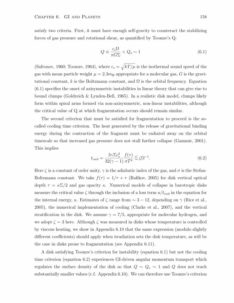
Chapter 6. GI and Planets 158
satisfy two criteria. First, it must have enough self-gravity to counteract the stabilizing
forces of gas pressure and rotational shear, as quantified by Toomre’s Q:
Q - cs%
.G$< Qo $ 1 (6.1)
(Safronov, 1960; Toomre, 1964), where cs =!
kT/µ is the isothermal sound speed of the
gas with mean particle weight µ = 2.3mH appropriate for a molecular gas, G is the gravi-
tational constant, k is the Boltzmann constant, and % is the orbital frequency. Equation
(6.1) specifies the onset of axisymmetric instabilities in linear theory that can give rise to
bound clumps (Goldreich & Lynden-Bell, 1965). In a realistic disk model, clumps likely
form within spiral arms formed via non-axisymmetric, non-linear instabilities, although
the critical value of Q at which fragmentation occurs should remain similar.
The second criterion that must be satisfied for fragmentation to proceed is the so-
called cooling time criterion. The heat generated by the release of gravitational binding
energy during the contraction of the fragment must be radiated away on the orbital
timescale so that increased gas pressure does not stall further collapse (Gammie, 2001).
This implies
tcool =30$c2
s
32(0 & 1)
f(1)
!T 4<$ 6%!1. (6.2)
Here 6 is a constant of order unity, 0 is the adiabatic index of the gas, and ! is the Stefan-
Boltzmann constant. We take f(1) = 1/1 + 1 (Rafikov, 2005) for disk vertical optical
depth 1 = )$/2 and gas opacity ). Numerical models of collapse in barotropic disks
measure the critical value 6 through the inclusion of a loss term u/tcool in the equation for
the internal energy, u. Estimates of 6 range from $ 3& 12, depending on 0 (Rice et al.,
2005), the numerical implementation of cooling (Clarke et al., 2007), and the vertical
stratification in the disk. We assume 0 = 7/5, appropriate for molecular hydrogen, and
we adopt 6 = 3 here. Although 6 was measured in disks whose temperature is controlled
by viscous heating, we show in Appendix 6.10 that the same expression (modulo slightly
di!erent coe#cients) should apply when irradiation sets the disk temperature, as will be
the case in disks prone to fragmentation (see Appendix 6.11).
A disk satisfying Toomre’s criterion for instability (equation 6.1) but not the cooling
time criterion (equation 6.2) experiences GI-driven angular momentum transport which
regulates the surface density of the disk so that Q $ Qo $ 1 and Q does not reach
substantially smaller values (c.f. Appendix 6.10). We can therefore use Toomre’s criterion

Chapter 6. GI and Planets 159
to define a relationship between $ and T at fragmentation, as a function of period:
$ =cs%
.GQo= fq
3T% (6.3)
where for convenience we define fq - (k/µ)1/2(.GQo)!1. We shall hereafter set Qo = 1.
Given equation (6.3), we can rewrite equation (6.2) to generate a single criterion for
fragmentation which depends on temperature and location:
%tcool
6= (fqft)
%2
T 5/2f(1) ' 1, (6.4)
where ft - (3/32)0(0 & 1)!1k(µ!6)!1. Somewhat counterintuitively, the critical cooling
constraint requires that a disk be su#ciently hot to fragment. The value of f(1) depends
on both % and T . Evaluating this criterion relies on the disk opacity, which we return to
in §6.4.2.
6.4 Minimum fragment masses and separations
6.4.1 Initial masses of GI-born fragments
We take the initial mass of a fragment to be the mass enclosed within the radius of the
most unstable wavelength, #Q = 2.H in a Q = 1 disk, or:
Mfrag ( 7(2.H)2 (6.5)
(Levin, 2007), where H = cs/% is the disk scaleheight. Cossins et al. (2009) have shown
that even when the GI is non-axisymmetric, the most unstable axisymmetric wavelength
#Q is one of the dominant growing modes, suggesting that this is a reasonable estimate.
While more numerical follow up will be necessary to pin down the true distribution of
fragments born through GI, at present simulations show that this estimate may well be a
lower limit, but is the correct order of magnitude (Boley, 2009; Stamatellos & Whitworth,
2009).
Using equation (6.3), we rewrite the fragment mass explicitly as a function of tem-
perature and location:
Mfrag ( 4.'
H
r
(3
M# = fmT 3/2
%(6.6)
where fm - (2.)2fqk/µ. Equation (6.6) demonstrates that at a given disk location, frag-
ment masses depend only on temperature, with lower temperatures generating smaller

Chapter 6. GI and Planets 160
fragments, subject to the minimum temperature required for fragmentation by equa-
tion (6.4).
Rafikov (2005) pointed out that there exists an absolute minimum fragment mass at
any disk location, when the disk satisfies the equalities in equation (6.1) and equation (6.2)
and has 1 = 1. The minimum temperature required for fragmentation scales as T %(1 +1/1)2/5 (equation 6.4), so the critical temperature and fragment mass are minimized
at 1 = 1, the optical depth for which cooling is most e#cient. The corresponding
minimum mass as a function of location is:
Mf,min = fm(fqft)3/5%1/5 (6.7)
= 1.5MJup
'r
100 AU
(!3/10%
M#
1.5M"
&1/10
(6.8)
which occurs for disk temperatures:
Tf,min = 7K'
r
100 AU
(!6/5%
M#
1.5M"
&2/5
(6.9)
Equation (6.7) corresponds to Q = 1, %tcool = 3, and 1 = 1. This minimum mass is only
achieved for temperatures consistent with Tf,min. Once an opacity law is specified which
relates T and 1 , the problem becomes overconstrained— these three criteria can only be
satisfied at a single disk location, and equations 6.7-6.9 are valid at only one radius in
the disk. We now proceed to evaluate the critical disk temperatures and fragment masses
for realistic opacity laws, demonstrating that planetary-mass fragments can only form at
large separations from their host star.
6.4.2 Opacity
At low temperatures, when T <$ 155 K, ice grains are the dominant source of opacity
(Pollack et al., 1985). Above $155 K, ices begin to sublimate. In the cold regime
applicable to the outer regions of protoplanetary disks, we consider two realistic opacity
laws, one which is characteristic of grains in the interstellar medium (ISM), and one
which is characteristic of grains that have grown to larger sizes due to processes within
the disk. We assume a Rosseland mean opacity which scales as
) ( )$T $ (6.10)
where the both the exponent, &, and the constant )$ are not well constrained in proto-
planetary disks. They depend on the number-size distribution and composition of the

Chapter 6. GI and Planets 161
dust grains, and on the dust-to-gas ratio. For ISM like grains, the Rosseland mean
opacity may be approximated by an opacity law with & = 2, or
) ( )2T2 (6.11)
(Pollack et al., 1996; Bell & Lin, 1994; Semenov et al., 2003) as long as the ice grains
dominating the opacity are smaller than a few tens of microns. This opacity law is
observationally confirmed in the ISM (Beckwith et al., 2000, and references therein). For
our fiducial model we use )2 ( 5 ) 10!4cm2/g for T in Kelvin, a fit to the standard
dust model by Semenov et al. (2003). Throughout, we quote ) per gram of gas for a
dust-to-gas ratio of 10!2.
As grains grow larger, they eventually exceed the wavelength of the incident radiation,
and so the opacity is determined by the geometric optics limit. In this case the Rosseland
mean opacity is independent of temperature, so the exponent & = 0. In this limit:
) ( )0 (6.12)
For a fixed dust mass in grains of size s, )0 % s!1. For our fiducial model we choose
)0 ( 0.24 cm2/g which is valid for T >$ 20 K and typical grain sizes of order 300µm (see
Figure 6 of Pollack et al., 1985).
Observations of emission from optically thin protoplanetary disks show evidence of
grain growth at millimeter wavelengths. Specifically the measured opacities )+ % ,,
with ( . 0.5—1.5 in the Rayleigh-Jeans tail imply particle growth toward the millimeter
wavelengths of the observations (D’Alessio et al., 2001). Although most observed disks
have had more time for grain growth to proceed, Class 0 sources also show evidence of
grain growth (D’Alessio et al., 2001). Alternatively, these objects could be optically thick
at millimeter wavelengths, which would mimic the e!ects of grain growth.
Using these opacity laws we see that cooling proceeds with a di!erent functional form
in the optically thick and optically thin limits. In the optically thick regime, f(1) (1 = ()$T $$)/2, which when combined with equation (6.4) indicates that to fragment,
the disk must have temperature
T >3ftf
2q /2
41/(2!$) 3%3)$
41/(2!$)(6.13)
for & 4= 2. In the special case & = 2, the fragmentation constraint is temperature-
independent, as discussed in §6.4.2.

Chapter 6. GI and Planets 162
In the optically thin regime, f(1) = 1/1 = 2/()$T $$). The cooling time is indepen-
dent of $, so we can rewrite equation (6.4) as:
T > (2ft)1/(3+$)
%%
)$
&1/(3+$)
, (6.14)
Fig. 6.1 shows the dependence of the cooling time on disk temperature for each opacity
law at two di!erent radii. Since fragmentation can only occur when %tcool < 6, the
minimum temperatures at which fragmentation is allowed are specified by the intersection
of the cooling curves with the %tcool boundary.
Small grain opacity law
For an optically thin disk with & = 2, equation (6.14) implies that in order to fragment,
the disk must have temperatures in excess of:
T > Tthin = 9K'
r
100 AU
(!3/10
(6.15)
%)2
5) 10!4cm2/g
&!1/5 %M#
1.5M"
&1/10
Colder disks, even when optically thin, cannot cool quickly enough to fragment.
For an optically thick disk, & = 2 turns out to be a special case: the temperature
dependence drops out of equation (6.13), giving instead a critical radius beyond which
fragmentation can occur, independent of the disk temperature:
r >$ 70 AU
%M#
1.5M"
&1/3 %)2
5) 10!4cm2/g
&!2/9
. (6.16)
Matzner & Levin (2005) first pointed out the existence of a minimum critical radius
for fragmentation. In Fig. 6.2 we illustrate how the two fragmentation criteria create a
radius rather than temperature cuto!. At radii larger than the critical radius defined
above, any $ & T combination which gives Q ' 1 will fragment (so long as the opacity
law remains valid). At smaller radii, no combination of $ and T which gives Q ' 1 will
fragment because the disk cannot simultaneously satisfy the cooling time criterion.
Large grain opacity law
As shown in Fig. 6.1, for the large grain opacity, 1 > 1 for all relevant temperatures. In
this case equation (6.13) requires:
T > 65K
%M#
1.5M"
&3/4 'r
43 AU
(!9/4%
)0
0.24 cm2/g
&1/2
. (6.17)

Chapter 6. GI and Planets 163
100
101
102
10!2
10!1
100
101
102
103
104
Temperature
! t
cool
"=0.24 g/ cm2
"=5 # 10!4
T2 g/ cm
2
40 AU 100 AU
R=40 AU
R=100 AUFragmentation $
Figure 6.1: The disk cooling time as a function of tempertature for di!erent opacity laws
at radii of 40 AU (dashed) and 100 AU (solid). The cooling time is calculated assuming
that Q = 1. The temperature independent (large grain) opacity law is shown in red, while
the ISM opacity law: ) % T 2 is shown in blue. The line thickness indicates the optical
depth regime. When lines drop below the critical cooling time (grey), disk fragmentation
can occur. The bend in the ISM opacity curve indicates that in the optically thick regime,
the cooling time becomes constant as a function of temperature.
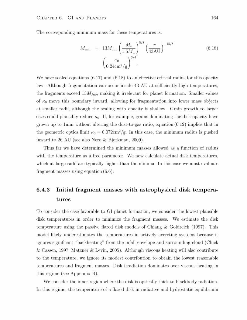
Chapter 6. GI and Planets 164
The corresponding minimum mass for these temperatures is:
Mmin = 13MJup
%M#
1.5M"
&5/8 'r
43AU
(!15/8
(6.18)
%)0
0.24cm2/g
&3/4
.
We have scaled equations (6.17) and (6.18) to an e!ective critical radius for this opacity
law. Although fragmentation can occur inside 43 AU at su#ciently high temperatures,
the fragments exceed 13MJup, making it irrelevant for planet formation. Smaller values
of )0 move this boundary inward, allowing for fragmentation into lower mass objects
at smaller radii, although the scaling with opacity is shallow. Grain growth to larger
sizes could plausibly reduce )0. If, for example, grains dominating the disk opacity have
grown up to 1mm without altering the dust-to-gas ratio, equation (6.12) implies that in
the geometric optics limit )0 = 0.072cm2/g. In this case, the minimum radius is pushed
inward to 26 AU (see also Nero & Bjorkman, 2009).
Thus far we have determined the minimum masses allowed as a function of radius
with the temperature as a free parameter. We now calculate actual disk temperatures,
which at large radii are typically higher than the minima. In this case we must evaluate
fragment masses using equation (6.6).
6.4.3 Initial fragment masses with astrophysical disk tempera-
tures
To consider the case favorable to GI planet formation, we consider the lowest plausible
disk temperatures in order to minimize the fragment masses. We estimate the disk
temperature using the passive flared disk models of Chiang & Goldreich (1997). This
model likely underestimates the temperatures in actively accreting systems because it
ignores significant “backheating” from the infall envelope and surrounding cloud (Chick
& Cassen, 1997; Matzner & Levin, 2005). Although viscous heating will also contribute
to the temperature, we ignore its modest contribution to obtain the lowest reasonable
temperatures and fragment masses. Disk irradiation dominates over viscous heating in
this regime (see Appendix B).
We consider the inner region where the disk is optically thick to blackbody radiation.
In this regime, the temperature of a flared disk in radiative and hydrostatic equilibrium

Chapter 6. GI and Planets 165
10 100Temperature (K)
1
10
100
1000
Su
rfac
e D
ensi
ty (
g/c
m2)
Q < 1
tc < 3 !!1
" < 1
a = 100 AU
10 100
1
10
100
1000
Figure 6.2: Fragmentation can only occur in the region of parameter space indicated by
the overlapping hashed regions for ISM opacities at radii of 100 AU. The upper, shaded
region (red) shows where Toomre’s parameter Q < 1. The lower, shaded region (blue)
indicates where tcool ' 3%!1. At radii less than 70 AU, fragmentation is prohibited be-
cause the two regions no longer overlap. That the boundaries of these regions are parallel
lines reflects the ) % T 2 form of the ice-grain-dominated opacity at low temperatures.

Chapter 6. GI and Planets 166
is:
Tm ='
(F
4
(1/4 'R#
r
(1/2
T# % L2/7r!3/7 (6.19)
where (F measures the grazing angle at which starlight hits the disk; (F is dependent on
the degree of disk flaring measured at the height of the photosphere (Chiang & Goldreich,
1997). Grain settling may reduce the height of the photosphere (set here to 4 times
the scaleheight) and thus (F . For the standard radiative equilibrium model, the disk
flaring scales approximately as H/r % r2/7. We shall find when we calculate the disk
temperature that a gravitationally unstable disk remains optically thick, justifying the
use of this formula.
To estimate the the stellar luminosity we use the stellar evolution models of Krumholz
& Thompson (2007), which include both nuclear burning and accretion energy. The
accretion luminosity depends on both the current accretion rate and the accretion history
( in so far as it e!ects the stellar radius), so we obtain the lowest luminosity estimates
by allowing the star to accrete at a constant, low accretion rate. We use the stellar
luminosity after accreting to 90% of its current mass (or 1.35M" assuming roughly 10%
is still in the disk). We choose an accretion rate of 10!7M"/yr as a lower bound because
a star accreting at a lower accretion rate throughout its history has a formation timescale
that is too long. Accretion rates an order of magnitude larger give comparable luminosity
(when the star has only reached 1.35M") to the present day luminosity of 5L" (Marois
et al., 2008). Lowering the accretion rate below this value does not significantly lower
the stellar luminosity because the accretion energy contribution is small.
The luminosity calculated for an accretion rate of 10!7M"/yr translates to tempera-
tures of:
T ( 40 K'
r
70 AU
(!3/7
, (6.20)
which we shall use as our fiducial temperature profile. In the outer regions of the disk
where fragmentation is allowed, the disk temperatures are of order 30& 50K. These tem-
peratures exceed the minimum threshold for fragmentation, and so the mass of fragments
will be set by equation (6.6).
Other analytic and numerical models of stellar irradiation predict temperatures in
agreement with or higher than our estimate. (Rafikov & De Colle, 2006; O!ner et al.,
2009b). Similarly, models of disks in Ophiuchus have similar temperatures for 1 Myr
old stars of lower mass (and thus luminosity), implying that our model temperatures are
low, though not unrealistic (Andrews et al., 2009).

Chapter 6. GI and Planets 167
20 40 60 80 100 120 14010
0
101
102
Radius (AU)
Tem
per
atu
re (
K)
d
b
. fragmentation !rcrit
for " # T2
c
Mfrag
Low M Model
Mfrag
(10 K)
! fragmentation, T > Tmin
100
101
M/M
jup
Temperature
102
Figure 6.3: Depiction of the current configuration of HR 8799 and formation constraints
for realistic disk temperatures. We show the lowest expected irradiated disk temperatures
(blue) and corresponding fragment masses (grey), as a function of radius. The lower
bound on both regimes (burgundy) is set by the irradiation model described in §6.4.3,
with M = 10!7M"/yr. The upper boundary is set by the current luminosity of HR
8799, $ 5L". The green dashed-dotted line shows the mass with disk temperatures
of 10 K, a lower limit provided by the cloud temperature. The vertical line shows the
critical fragmentation radius for the ISM opacity law; fragmentation at smaller radii
requires grain growth. Fragment masses are shown for radii at which the irradiation
temperatures are high enough to satisfy the cooling time constraint of equation (6.17).
At smaller radii, fragmentation is possible at higher disk temperatures, but the resulting
fragments have correspondingly higher masses, and planet formation is not possible.

Chapter 6. GI and Planets 168
In Fig. 6.3 we illustrate the constraints on fragment masses from this irradiation
model, calculated using equation (6.6). We show the fiducial disk temperatures of equa-
tion (6.20), along with temperatures consistent with luminosities up to the present-
day luminosity. For our fiducial opacity laws, the expected fragment masses are only
marginally consistent with GI planet formation— fragments form near the upper mass
limit of 13MJup. Lower opacities produced by grain growth might allow fragmentation
into smaller objects at closer radii. Whether grain-growth has proceeded to this extent
in such young disks is unclear.
6.5 Growth of fragments after formation
For realistic disk temperatures, it is conceivable that fragments may be born at several
MJup. We now consider their subsequent growth, which may increase their expected mass
by an order of magnitude or more.
The final mass of a planet depends sensitively on numerous disk properties (e!ective
viscosity, column density, scaleheight) and the mass of the embedded object. In order
to constrain the mass to which a fragment will grow, we can compare it to two relevant
mass scales: the disk isolation mass and the gap opening mass.
Halting the growth of planetary mass objects is a relevant problem independent of
the formation mechanism. However the GI hypothesis requires that the disk is (or was
recently) su#ciently massive to have Q $ 1, implying that the disk is actively accreting.
The core accretion scenario does not face this restriction.
6.5.1 Isolation Mass
We estimate an upper mass limit for fragments by assuming that they accrete all of the
matter within several Hill radii:
Miso ( 4.fH$RHr. (6.21)
Here fH $ 3.5 is a numerical constant representing from how many Hill radii, RH =
r(Miso/3M#)1/3, the planet can accrete (Lissauer, 1987).
It is instructive to compare the ratio of the isolation mass to the stellar mass:
Miso
M#= 4.6f 3/2
H Q!3/2'
H
r
(3/2
. (6.22)

Chapter 6. GI and Planets 169
1 10
Q
0.01
0.10
H/R
0.003
0.010
0.030
0.030
0.100
0.100
0.300
1.000
Figure 6.4: Contours of the ratio of planetary isolation mass to stellar mass as a function
of Toomre’s Q and the disk aspect ratio H/r, illustrating that the isolation mass is always
large in unstable disks. For disks with higher Q’s consistent with core accretion models,
the isolation mass remains small. The shaded region indicates where the isolation mass
exceeds the stellar mass.
We find that large isolation masses are always expected in gravitationally unstable disks.
Fig. 6.4 illustrates the scaling of equation (6.22) with Q and the disk aspect ratio, H/r.
For our fiducial temperature profile, H/r ( 0.09 at 70 AU. For low values of Q and
comparable H/r, the isolation mass exceeds 10% of the stellar mass. For the ideal disk
values cited above (equation 6.16), the isolation mass is:
Miso ( 400MJup
'r
70 AU
(6/5%
M#
1.5M"
&1/10
. (6.23)
This mass is nearly two orders of magnitude larger than the minimum mass. Growth
beyond the isolation mass is possible either through mergers or introduction of fresh
material to accrete by planet migration or disk spreading.
Objects which grow to isolation mass cannot be planets, and so we turn to mechanisms
that truncate fragment growth below the isolation mass.

Chapter 6. GI and Planets 170
6.5.2 Gap opening mass
Massive objects open gaps in their disks when gravitational torques are su#ciently strong
to clear out nearby gas before viscous torques can replenish the region with new material.
(Lin & Papaloizou, 1986; Bryden et al., 1999). The gap width is set by the balance
between the two torques:
'
r=
%fgq2
3.(
r2
H2
&1/3
, (6.24)
where ' is the gap width, fg ( 0.23 is a geometric factor derived in Lin & Papaloizou
(1993), q is the planet to star mass ratio, and ( is the Shakura & Sunyaev (1973)
e!ective viscosity. This can be used to derive the standard minimum gap opening mass
by requiring that ' > H:
q >'
H
r
(5/2:
3.(
fg(6.25)
( 4) 10!3'
(
0.1
(1/2 'T
40 K
(5/4 'r
70 AU
(5/4
%M#
1.5 M"
&!5/4
.
Gap opening requires ' > RH and RH > H. The latter requirement is automatically
satisfied for fragments formed by GI.
While the e!ects of GI are often parameterized through an ( viscosity, Balbus &
Papaloizou (1999) have pointed out that (, a purely local quantity, may not adequately
describe GI driven transport, which is inherently non-local. Lodato & Rice (2005) have
shown that for su#ciently thin disks, the approximation is reasonable: in order to form
objects of planetary mass, the disk must be relatively thin and at least marginally within
this limit. However, even in this thin-disk limit, it is not clear that GI driven torques
will exactly mimic viscous ones at gap-opening scales.
Equation (6.25) implies that the gap opening mass is less than or equal to the fragment
mass for e!ective viscosities consistent with GI. We use ( ( 0.1, as this is consistent with
active GI (Gammie, 2001; Lodato & Rice, 2005; Krumholz et al., 2007b). If the local
disk viscosity is lower, fragments will always form above the gap-opening mass.

Chapter 6. GI and Planets 171
Gap-opening starvation mass
Gap-opening slows accretion onto the planet, but does not starve it of material com-
pletely. Accretion rates through gaps remain uncertain for standard core accretion mod-
els, and numerical models are not available for accretion onto the distended objects
formed through GI fragmentation. Nevertheless simulations of accretion through gaps
in low viscosity disks (Lubow et al., 1999) demonstrate that accretion is slower through
larger gaps, and this qualitative conclusion likely remains valid as long as gaps form.
Analogous to the isolation mass, we consider a “gap starvation mass” that is related
to the ratio of the gap width to planet Hill radius. Rewriting equation (6.24) we find the
ratio of gap width to Hill radius is:
'
RH=
%fgq
.(
r2
H2
&1/3
(6.26)
Note that ' > RH recovers the canonical gap opening estimate appropriate for Jupiter:
q > 40,/(r2%), modulo order unity coe#cients (cf. Crida et al., 2006).
If we make the simplifying assumption that gap accretion terminates when the gap
width reaches a fixed number of Hill radii, fS, we can calculate a gap starvation mass. We
expect that for a gap to truncate accretion, fS>$ fH = 3.5, the width in Hill radii used to
calculate the isolation mass (§6.5.1). Terminating accretion is an unsolved problem for
Jupiter in our own solar system, and so to provide a further constraint on fS, we refer
to the numerical simulations of Lissauer et al. (2009) (See also D’Angelo et al. (2003) for
a detailed explanation of the numerical work). Their runs 2l and 2lJ exhibit asymptotic
mass growth after $2.5 Myr for a constant-mass, low viscosity (( = 4)10!4) disk under
conditions appropriate to the formation of Jupiter. Using equation (6.26), we solve for
the width of the gap generating this fall-o! in accretion rate and find fS = '/RH $ 5.
The need for an extremely large and well-cleared gap reflects the integrated e!ects of
low-level accretion through the gap and onto the planet over the disk lifetime of a few
Myr. Even a slow trickle of material onto the planet can contribute to significant growth.
Using fS = 5, the gap-opening starvation mass for HR 8799 scaled to both the
simulated solar-system viscosity and to the expected GI viscosity is:
Mstarve ( 8MJup
'(
4) 10!4
( ''
5RH
(3
(6.27)'
T
40 K
( 'r
70 AU
(

Chapter 6. GI and Planets 172
( 2000MJup
'(
0.1
( ''
5RH
(3
'T
40 K
( 'r
70 AU
(.
In order to limit growth to planetary masses, the e!ective viscosity must be two orders
of magnitude below that expected in GI unstable disks, roughly ( $ 10!3. More restric-
tively this requires that other local transport mechanisms such as the MRI be weaker
than currently predicted by simulations—they produce ( $ 10!2 at least in disks with
a net magnetic flux (Fleming et al., 2000; Fromang et al., 2007; Johansen et al., 2009).
Fig. 6.5 illustrates the scaling of gap starvation mass with radius for several values of
(. It appears that active disks face severe obstacles in producing planetary mass objects
unless the disk disappears promptly after their formation. Although we expect fragmen-
tation to make the disk more stable by lowering the local column density, there is little
reason to expect a recently massive disk to be so quiescent.
Planet starvation through gap overlap
Although it is unlikely that the disk will fragment into a su#ciently large number of
planetary mass objects to completely deplete the disk of mass (Stamatellos & Whit-
worth, 2009), the formation of multiple fragments simultaneously may limit accretion
through competition for disk material by opening overlapping gaps. The current separa-
tion between the planets is such that gaps larger than roughly three Hill radii overlap,
so depending on their migration history, this could limit growth (see also §6.7). From
equation (6.27) we see that if gaps are forced to be smaller by a factor of two due to com-
petition with another planet, the expected masses are decreased by a factor of 8. This
e!ect would imply that fragments in multiple systems should be lower in mass. Note
that when simulated disks fragment into multiple objects simultaneously, they generally
have orbital configurations like hierarchical multiples rather than planetary systems (Sta-
matellos & Whitworth, 2009; Kratter et al., 2010). Whether the same conditions required
to limit fragment growth—reduced disk mass and/or viscosity after fragmentation—can
allow the retention of a planetary system of fragments remains to be simulated.
6.5.3 Disk dispersal as a means to limit fragment growth
Mechanisms for gas dispersal such as photoevaporation may be necessary to stunt plan-
etary growth, even for models of Jupiter in our own solar system (Lissauer et al., 2009).

Chapter 6. GI and Planets 173
10 100Radius (AU)
1
10
100
1000
M/M
jup
Figure 6.5: The gap starvation mass as a function of disk radius. We show curves for
several values for (, and indicate the planetary mass regime, and the region in which disk
fragmentation is likely. We use fS = 5, scaled to simulation 2lJ of Jupiter formation in
Lissauer et al. (2009) (labeled L09 in the figure). The radial scaling is derived assuming
H/r % r2/7. For the low viscosity case, we normalize the scale height to Jupiter at 5.2
AU in a 115 K disk for comparison with L09. For the higher viscosities, we normalize the
disk scale height to the lowest expected temperatures (equation 6.20). For comparison
we show the HR 8799 planets as black circles.
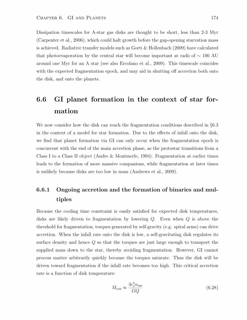
Chapter 6. GI and Planets 174
Dissipation timescales for A-star gas disks are thought to be short, less than 2-3 Myr
(Carpenter et al., 2006), which could halt growth before the gap-opening starvation mass
is achieved. Radiative transfer models such as Gorti & Hollenbach (2009) have calculated
that photoevaporation by the central star will become important at radii of $ 100 AU
around one Myr for an A star (see also Ercolano et al., 2009). This timescale coincides
with the expected fragmentation epoch, and may aid in shutting o! accretion both onto
the disk, and onto the planets.
6.6 GI planet formation in the context of star for-
mation
We now consider how the disk can reach the fragmentation conditions described in §6.3
in the context of a model for star formation. Due to the e!ects of infall onto the disk,
we find that planet formation via GI can only occur when the fragmentation epoch is
concurrent with the end of the main accretion phase, as the protostar transitions from a
Class I to a Class II object (Andre & Montmerle, 1994). Fragmentation at earlier times
leads to the formation of more massive companions, while fragmentation at later times
is unlikely because disks are too low in mass (Andrews et al., 2009).
6.6.1 Ongoing accretion and the formation of binaries and mul-
tiples
Because the cooling time constraint is easily satisfied for expected disk temperatures,
disks are likely driven to fragmentation by lowering Q. Even when Q is above the
threshold for fragmentation, torques generated by self-gravity (e.g. spiral arms) can drive
accretion. When the infall rate onto the disk is low, a self-gravitating disk regulates its
surface density and hence Q so that the torques are just large enough to transport the
supplied mass down to the star, thereby avoiding fragmentation. However, GI cannot
process matter arbitrarily quickly because the torques saturate. Thus the disk will be
driven toward fragmentation if the infall rate becomes too high. This critical accretion
rate is a function of disk temperature:
Mcrit (3c3
s(sat
GQ(6.28)

Chapter 6. GI and Planets 175
(Gammie, 2001; Matzner & Levin, 2005). Numerical simulations show that GI saturates
at (sat $ 0.3& 1 (Gammie, 2001; Krumholz et al., 2007b; Lodato & Rice, 2005; Kratter
et al., 2010). If the infall rate onto the disk exceeds Mcrit the disk can no longer regulate
the surface density to keep Q just above unity, and fragmentation will occur. Because the
conversion of accretion energy to thermal energy at large radii is ine#cient, disks cannot
restabilize through heating to arbitrarily high accretion rates (Kratter & Matzner, 2006).
If fragmentation occurs due to rapid accretion, as described above, it is di#cult to
limit subsequent fragment growth. As demonstrated in §6.5.2, gap opening does not limit
accretion e#ciently when the e!ective viscosity, in this case, (sat, is high.
A more general barrier to making small fragments during rapid infall is the large
reservoir of material passing by the fragment as star formation proceeds (Bonnell &
Bate, 1994a). The specific angular momentum, j, of accreting disk material typically
increases with time (modulo small random fluctuations in a turbulent core), landing at
a circularization radius, rcirc = j2/GM#, which is larger than the fragment’s orbit. Since
the fragment’s Hill radius is roughly 10% of the disk radius, newly accreted material
undergoes many orbits in the fragment’s sphere of influence as it tries to accrete onto
the central star, and some fraction will accrete onto the fragment itself. This process
is less e#cient if global GI modes drive fragments to smaller radii, because their Hill
radii shrink. However, growth to stellar (or sub-stellar) masses may still occur as long as
migration timescales are not faster than accretion timescales. The latter scenario implies
that the disk cannot fragment at early times and still reproduce a single-star system like
HR 8799.
The trend toward continued growth and even mass equalization following disk frag-
mentation is observed in numerous simulations with ongoing accretion (Bonnell & Bate,
1994a; Bate, 2000; Matsumoto & Hanawa, 2003; Walch et al., 2009b; Kratter et al., 2010;
Krumholz et al., 2009). Simulations of planet formation by GI with ongoing accretion
also illustrate this behavior (Boley, 2009).
Consequently, if the HR 8799 planets formed by GI, they must have fragmented at the
tail end of accretion from the protostellar core onto the disk. Most likely, this requires
that the protostellar core have properties such that its infall rate reaches the critical value
in equation (6.28) just as the core is drained of material. If this coincidence in timing
does not occur, fragmentation produces a substellar, rather than a planetary, companion.
Whether fragmentation at this epoch can produce non-heirarchical orbits like HR 8799
remains to be explored.

Chapter 6. GI and Planets 176
6.6.2 Reaching Instability in the absence of infall: FU Orionis
outbursts
Driving the disk unstable with external accretion corresponds to excessive growth of
fragments. It is therefore tempting to consider mechanisms to lower Q through disk
cooling, while holding the column density fixed. Because the disks are dominated by
irradiation, changes in the viscous dissipation due to accretion are unlikely to a!ect a
significant temperature change, and so lowering Q requires order of magnitude changes
in the stellar luminosity due to the weak scaling of T % L2/7. FU Orionis type outbursts
(Hartmann & Kenyon, 1996) can cause rapid changes in luminosity. To result in planetary
mass fragments, the luminosity drop following an FU Ori outburst would need to reach
at least the minimum luminosity used in equation (6.20) on timescales shorter than an
outer disk dynamical time.
The accretion of GI formed embryos onto the protostar is a proposed source of the
outbursts (Vorobyov & Basu, 2006). If this occurs, perhaps a final generation of gravi-
tational fragments, the so-called “last of the Mohicans” (Gonzalez, 1997), would remain
as detectable companions. Although the lack of infall in this scenario might ease the
gap opening constraints, fragments face all of the other di#culties discussed above in
remaining low in mass.
6.7 Migration in a multi-planet system
A final consideration for making wide orbit planets through GI is their subsequent mi-
gration history. If formed via GI, the HR 8799 planets had to migrate inward to their
current locations. There is an independent reason to believe that migration did in fact
take place in this system. As discussed by Fabrycky & Murray-Clay (2008), the long
term stability of HR 8799 requires a resonant orbital configuration, most plausibly a
4:2:1 mean motion resonance, which likely resulted from convergent migration in the
protoplanetary gas disk. We demonstrate below that while this history is plausible, it
requires special disk conditions.
Inward Type II migration (appropriate for gap opening planets) is expected at for-
mation, because the fragmenting region is within the part of the disk accreting onto the

Chapter 6. GI and Planets 177
star. Type II migration of a single planet occurs on the disk viscous timescale:
1+ ( r2
,=
r2%
(c2s
(6.29)
( 0.4 Myr'
r
70 AU
(13/14%
M#
1.5M"
&1/2 '(
0.1
(!1
(6.30)
where we have used , = (c2s/%. This timescale is short enough to allow substantial
migration during the lifetime of the gas disk.
If fragments migrated inward independently, they could never become captured in
resonance, as the innermost planet would migrate farther and farther from its neighbor.
However, as shown in §6.5, planetary gaps may overlap if they are within several Hill
radii of each other, comparable to the current separations between the HR 8799 planets.
This overlap alters the torques felt by, and thus the migration of, the planets. As shown
by Kley (2000), if multiple planetary gaps interact, convergent migration is possible.
Gap interaction allows an outer planet to shield an inner planet from the material, and
thus torques, of the outer disk, slowing or halting its inward migration and allowing the
outer planet to catch up. This mechanism is invoked by Lee & Peale (2002) to generate
convergent migration and resonance capture in the planets orbiting GJ 876.
Under the assumption that gap overlap allows convergent migration and resonance
capture, we now ask: What is the overall direction of the subsequent migration? We note
that if the planets migrated a substantial distance after resonance capture, eccentricity
damping by the gas disk was likely necessary (c.f., Lee & Peale, 2002). We do not
consider eccentricity damping further here. Once two planets are caught in mean-motion
resonance, the torque on an individual planet from the gas disk can cause both planets
to migrate, with angular momentum transfer mediated by the resonance. Masset &
Snellgrove (2001) (see also Crida et al., 2009) have argued that the torque imbalance
on a pair of gap-opening resonant planets can even reverse the direction of migration,
although this relies on a significant di!erence between planet masses.
Nevertheless, understanding the planets’ overall migration requires understanding
how overlapping gaps alter the torque balance on the group of planets. Guided by our
interest in clean gaps that limit the growth of planets (§6.5–6.6), we consider the following
simplified problem.
We imagine that the three planets have cleared, and are embedded in, a single large
gap which is su#ciently clean that any disk gas passing through is dynamically unim-
portant. Because the system is locked in a double mean-motion resonance, we assume

Chapter 6. GI and Planets 178
that an imbalance in the torques acting on the two edges of the gap can cause all three
planets to migrate. We can then ask: is there a su#cient flux of angular momentum
from the outer disk to cause the planets to migrate inward with the viscous accretion of
the disk?
When in the 4:2:1 resonance, the total angular momentum of the planets is roughly
2.4Mp%pr2p, where we have assumed that the planets are roughly equal in mass, Mp, while
rp and %p are the separation and Keplerian angular velocity of the outermost planet. The
angular momentum flux from the outer disk is large enough to move the planets on a
viscous time r2p/, when:
M%pr2p>$ 2.4Mp%pr
2p(,/r2
p) , (6.31)
where M = 3.$, is the mass flux through radius rp.
Using the above inequality, we can calculate a critical disk surface density at the
current location of the outer planet such that the disk can push the planets inward:
$ >$Mp
4r2p
. (6.32)
For Mp = 10MJup and our fiducial disk temperatures (equation 6.20), this constraint
is always satisfied when Q = 1. The disk is unable to cause inward migration when
$ <$ 4g/cm2 at 70 AU, which is equivalent to Q $ 20.
If the planets do share a clean common gap, a large fraction of the disk would be
e!ectively cleared of gas while a massive outer disk is still present. A similar mechanism
has been invoked to explain transitional disks, which contain holes at radii of a few tens
of AU and smaller (Calvet et al., 2002). Transport of disk gas through a less well-cleared
gap could substantially alter this picture.
In summary, it is possible to envision a scenario in which the HR 8799 planets migrate
inward to their current locations in such a way that their orbits converge, allowing reso-
nance capture. This scenario is consistent with other constraints on GI planet formation:
shortly after formation, the disk must have low accretion rates and decline in mass in
order to (a) limit the growth of fragments, (b) allow for large, overlapping gaps.
More stringent constraints will require future work on migration in gravitationally
unstable disks, particularly in the presence of multiple planets massive enough to clear
large, overlapping gaps.

Chapter 6. GI and Planets 179
100 102 104
rp (AU)
10!4
10!3
10!2
10!1
100
Mp/M
*
10!2 100 102
rp/rcrit
10!2
10!1
100
101
102
Mp/M
frag
,min
Figure 6.6: (Left) Known substellar companions (stars) and planets (plusses) as a func-
tion of mass ratio and projected separation. The three objects in the HR 8799 system
are shown by pink circles, and a pink triangle denotes the upper-limit mass ratio for Fo-
malhaut b based on the dynamical mass estimate of Chiang et al. (2009). Grey squares
indicate the gap regions. Ongoing surveys are necessary to determine whether there
is a continuous distribution between Jupiter/Saturn (blue diamonds) and HR 8799, or
HR 8799 and brown dwarf companions. Planets around very low mass primaries with
M# = 0.02–0.1M" are marked by purple squares. These systems have mass ratios more
akin to the substellar companions than to the remainder of the population of planets.
Primary masses range from M# = 0.02M"–1M" (black) and M# = 1M"–2.9M" (red) for
substellar companions and from M# = 0.1–0.4M" (purple) and M# = 0.4–4.5M" (black)
for planets. (Right) The same objects plotted as function of the minimum fragment
mass, Mfrag,min and critical radius, rcrit. We use equation (6.16) to calculate rcrit. For
Mfrag,min, we apply equation (6.6) at radius rcrit under the simplified assumption that the
disk temperature is set by the stellar luminosity: L/L" = (M#/M")3.5 for M# > 0.43M"
and L %M2.3# for lower-mass stars. The temperatures used to calculate fragment masses
are not allowed to dip below 20K. Masses below Mfrag,min are unlikely to result from GI.

Chapter 6. GI and Planets 180
6.8 Current Observational Constraints
While there is a regime of parameter space in which planet formation is possible, typical
conditions produce more massive (> 13MJup ) companions. If GI fragmentation ever
forms planets, then fragmentation should typically form more massive objects. Conse-
quently, these planets would constitute the low mass tail of a distribution of disk-born
companions. If the mass distribution is continuous there should be more sub-stellar com-
panions than planets at comparable distances of 50-150 AU. Observing this population
is a strong constraint on the formation mechanism, but current data are insu#cient to
draw conclusions.
Zuckerman & Song (2009) have compiled the known sub-stellar companions in this
range of radii to date. This range of separations falls beyond the well-established inner
brown dwarf “desert” (McCarthy & Zuckerman, 2004), and has not been well probed
due to observational di#culties at these low mass ratios. Note that the overall dearth
of brown dwarf companions to solar mass stars is not a selection e!ect (Metchev &
Hillenbrand, 2009; Zuckerman & Song, 2009).
We illustrate the observational constraints by plotting the companions from Zucker-
man & Song (2009) along with the known exoplanets compiled by the Exoplanet En-
cyclopedia1 as a function of mass ratio and projected separation in Fig. 6.6a, and as a
function of minimum fragment masses and fragmentation radii in Fig. 6.6b. We compare
these with the HR 8799 planets, Fomalhaut b, and the solar system giants. We distin-
guish between stars of di!erent masses because disk fragmentation becomes more likely
for higher mass stars (Kratter et al., 2008).
At present, neither the population of substellar companions nor the population of
exoplanets is continuous out to HR 8799. Many selection biases are reflected in Fig. 6.6,
and these gaps in particular may be due to selection e!ects; resolution and sensitivity
make it di#cult to detect both wide orbit planets, and close-in low mass brown dwarfs.
We note that while there are actually fewer planets at distances less than 1 AU, the cuto!
above 5 AU is unphysical. There is not yet any indication of an outer cut o! radius in
the exoplanets: if they continued out to larger separation, the distribution would easily
encompass the HR 8799 and Fomalhaut systems.
Data from ongoing surveys like that which found HR 8799 are necessary to verify
the true companion distribution as a function of mass and radius. If these planets are
1October 2009, http://exoplanet.eu, compiled by Jean Schneider

Chapter 6. GI and Planets 181
formed through GI, we would expect observations to fill in the gap between HR 8799
and higher mass ratio objects to show a continuous distribution. If these planets are
formed via core accretion, than observations may fill in the plot on the opposite side of
HR 8799, occupying a region of parameter space for which neither core accretion nor GI
is currently a successful formation mechanism.
6.9 Summary
We have demonstrated that while GI-driven fragmentation is possible at wide distances
from A stars, fragment masses typically exceed the deuterium burning “planet” limit.
In contrast, the formation of sub-stellar and stellar companions is more likely because
moderate disk temperatures and active accretion onto and through the disk drive disk-
born objects to higher masses.
If the HR 8799 planets did form by GI, the following criteria had to be met:
1. Fragments should form beyond 40& 70 AU: inside of this location the disk will not
fragment into planetary mass objects even if Q <$ 1. Grain growth is required for
fragmentation at the lower end of this range.
2. Temperatures must be colder than those of typical disks to limit the initial fragment
masses.
3. The disk must be driven unstable at a special time: infall onto the disk must be
low, but the disk must remain massive (e.g. the end of the Class I phase). The disk
must only become unstable to fragmentation at this point because earlier episodes
of instability should lead to sub-stellar or stellar companion formation.
4. The subsequent growth of fragments must be limited through e#cient gap clearing
necessitating low disk viscosity or early gap overlap. Disk dispersal via photoevap-
oration may also be necessary.
5. The three fragments must form at the same epoch separated by several Hill radii,
implying that the entire outer disk becomes unstable simultaneously.
6. Migration must be convergent. This likely requires the gaps of the planets to overlap
so as to starve the inner most planet of disk material, thereby preventing runaway
inward migration.

Chapter 6. GI and Planets 182
If these conditions are met, then the planets in HR 8799 could comprise the low-mass
tail of the disk-born binary distribution, the runts of the litter. In this case one would
expect to find a larger number of brown dwarfs or even M stars in the same regime of
parameter space – surrounding A-stars at distances of 50& 150 AU.
Ongoing direct imaging surveys of A and F stars will provide a strong constraint
on the formation mechanism for this system: if HR 8799 is the most massive of a new
distribution of widely separated planets, our analysis suggests that formation by GI is
unlikely. On the contrary, the discovery of a population of brown dwarf and M-star
companions to A-stars would corroborate formation via disk fragmentation.
6.10 Appendix A. Cooling and Fragmentation in Ir-
radiated disks
Rafikov (2009) has suggested that the cooling time might be altered in an irradiated disk.
Here we consider the cooling time for thermal perturbations to a disk, and show that a
simple formula [equation (6.39)] gives the cooling time for arbitrary levels of irradiation,
at least in radiative optically thick disks.
Consider ambient radiation striking an optically thick disk with a normal flux Fo =
!T 4o - (3/8)Firr (where the numerical factor in the last definition is purely for later
convenience). Note that To depends both on the irradiation field (from the host star
and/or light emitted and reflected from a surrounding envelope) and also on the disk’s
surface geometry, e.g. flaring angle. By incorporating these variables into To we attempt
a general calculation. At the photosphere, where the optical depth to the disk’s self-
emission 1 = 1phot ( 1, energy balance gives:
!T 4e" . !T 4
o + F/2 . (6.33)
Here, F is the luminous flux from any internal sources of energy dissipation, e.g. viscous
accretion, shocks, or the gravitational binding energy released by a collapsing fragment.
The factor of two reflects that half of the radiation is emitted from each surface of the
disk. Since optical light is absorbed above the IR photosphere, about half the irradiation
free streams out before it heats the disk (Chiang & Goldreich, 1997). We can absorb this
reduction into the definition of To.

Chapter 6. GI and Planets 183
We assume heat is transferred by radiative di!usion as:
4
3!
dT 4
d1=
F
2. (6.34)
since convection is suppressed by irradiation and may be a negligible correction in any
event (Rafikov, 2007). Integration from the midplane at 1 = 1tot and T = Tm to the
photosphere gives:
(4/3)!(T 4m & T 4
e") = (F/2)(1tot & 1phot) . (6.35)
We now drop the subscripts from 1tot and the midplane Tm, which we will soon take as
the characteristic temperature (ignoring order unity corrections from height averaging).
Furthermore we apply equation (6.33) and take the 1phot , 1tot * 1 limit (meaning that
we don’t need to know the precise location of the photosphere) to express
F . 8!
31(T 4 & T 4
o ) =1
1
%8!T 4
3& Firr
&
, (6.36)
which shows that the midplane temperature is controlled by the larger of F 1 and Firr.
The cooling timescale to radiate away thermal fluctuations (generated e.g. by GI) is
tcool =$*U
*F(6.37)
where a temperature perturbation *T has an excess heat *U ( cP *T , and cP = (k/µ)0/(0&1) is the specific heat for a mean molecular weight µ and adiabatic index 0. Strongly
compressive motions, which are not at constant pressure, will introduce order unity cor-
rections that we ignore.
The excess luminous flux, using equation (6.36), is
*F =8!
31
*T
T
;(4& &)T 4 + &T 4
o
<
=32!T 3*T
31)
/1
2(1& &/4) if T + To, & 4= 4
1 if T . To
, (6.38)
where 1 = )$/2 % T $. The point is that the escaping flux varies by only an order unity
factor between the strongly (T . To) and weakly (T + To) irradiated regimes. Typical
grain opacities, 0 < & < 2, ensure the correction is order unity (and also ensure that we
can ignore the catastrophic heating that would occur if & > 4).
Combining equations (6.37) and (6.38) with the definition of heat capacity we find
that the cooling time is simply
tcool (30$c2
s1
32(0 & 1)!T 4)
/1
2(1& &/4)!1 if T + To, & 4= 4
1 if T . To
, (6.39)

Chapter 6. GI and Planets 184
where the isothermal sound speed cs =!
kT/µ.
From this derivation, we see that the cooling time obeys the simple form of equa-
tion (6.39) for all levels of irradiation — which only introduces an order unity & correc-
tion. The cooling time depends on & for weakly irradiated disks because changes to the
opacity alter the amount of flux that escapes from the midplane. In highly irradiated
disks, opacity changes have little e!ect because the small di!erence between the midplane
and surface temperatures drives a weak flux.
While increasing the irradiative flux incident on a disk decreases the cooling time by
raising T , it will not trigger fragmentation in a Q $ 1 disk, since it increases Q. We will
not explore optically thin or convective disks at this time.
We assume that %tcool < 6 $ 3 is the fragmentation criterion independent of ir-
radiation. When the cooling time is longer, the disk is presumed to enter a state of
gravito-turbulence (Gammie, 2001). We take this term to mean a quasi-steady state
of gravitationally driven turbulence, on scales <$H wherein viscous dissipation of GI
turbulence regulates Q $ 1. Thus the cooling time can be translated to a the critical
value of ( at which gravito-turbulent accretion disks will fragment. While Rice et al.
(2005) find that an (-threshold is more robust than one for tcool when the adiabatic index
varies, they did not include irradiation, which we contend would reveal that cooling is
ultimately the more physical criterion, but the issue is best settled by simulation. The
emitted flux with an (-viscosity and Q $ 1 gives
F ( (9/4),$%2 ( 9/(4.)(c3s%
2/G (6.40)
which combined with equation (6.36) and equation (6.39) without the & correction gives
%tcool (%
0
0 & 1
&%$c2
s
4 (F + Firr/1)(
%0
0 & 1
&1
9(
'1 +
Firr
F 1
(!1
(6.41)
When irradiation is weak enough that Firr<$ F 1 , we recover the standard ( >$ 1 crite-
rion for fragmentation (ignoring the accumulated order unity coe#cients). However for
stronger irradiation with Firr>$ F 1 , fragmentation occurs for ( >$ F 1/Firr, a lower thresh-
old.
Gravito-turbulent models require modification when Firr>$ F , i.e. an even lower level
of irradiation than needed to a!ect the ( fragmentation threshold. In this case the disk
shows some similarities to isothermal disks, and should have lower amplitude density per-
turbations, because there is insu#cient viscous dissipation to support order unity thermal

Chapter 6. GI and Planets 185
perturbations (see the related discussion in Rafikov, 2009). We note that simulations of
isothermal disks do develop GI, exhibit GI-driven transport and fragment (Krumholz
et al., 2007b; Kratter et al., 2010), but they do not appear particularly turbulent.
6.11 Appendix B. Temperature due to Viscous Heat-
ing
We now show that viscous heating is relatively unimportant in the outer reaches of
irradiated A-star disks (see also section 3 of Rafikov 2009). For an optically thick disk
with an ISM opacity law, balancing viscous heating and emitted radiation gives
8
31!T 4 ( 3
8.M82 (6.42)
The solution for the midplane temperature is
T (+
, 9
128.2
M)o
!k/µ
!GQo
-
.2/3
82 ( 9 K
%M
10!6M"/yr
&2/3
Q!2/3o
'r
70 AU
(!3
, (6.43)
lower than the irradiation temperatures shown in Fig. 6.3 by more than a factor of four.
Note that the surface density fallo!
7 =cs8
.GQo( 35 g/cm2
'r
70 AU
(!3%
M
10!6M"/yr
&1/3
(6.44)
is also quite steep for a constant Q0 = 1, viscous disk with the ISM opacity law.
If the disk is optically thin, then the balance between heating and cooling gives:
41!T 4 ( 3
8.M82 (6.45)
T (+
, 3GMQo8
16!)o
!k/µ
-
.2/13
(6.46)
( 9 K
%M
10!6M"/yr
&2/13 %M#
1.5M"
&1/13
Q2/13o
'r
70 AU
(!3/13
(6.47)
This temperature profile is shallow, but still colder than the irradiation temperature at
large radii where the disk becomes optically thin.

Bibliography
Adams, F. C., Lada, C. J., & Shu, F. H. 1987, ApJ, 312, 788
Adams, F. C., Proszkow, E. M., Fatuzzo, M., & Myers, P. C. 2006, ApJ, 641, 504
Adams, F. C., Ruden, S. P., & Shu, F. H. 1989, ApJ, 347, 959
Andre, P., & Montmerle, T. 1994, ApJ, 420, 837
Andre, P., Ward-Thompson, D., & Barsony, M. 1993, ApJ, 406, 122
Andrews, S. M., & Williams, J. P. 2007, ApJ, 659, 705
Andrews, S. M., Wilner, D. J., Hughes, A. M., Qi, C., & Dullemond, C. P. 2009, ApJ,
700, 1502
Anglada, G., Rodrıguez, L. F., Osorio, M., Torrelles, J. M., Estalella, R., Beltran, M. T.,
& Ho, P. T. P. 2004, ApJ, 605, L137
Artymowicz, P., & Lubow, S. H. 1996, ApJ, 467, L77+
Aumann, H. H., Beichman, C. A., Gillett, F. C., de Jong, T., Houck, J. R., Low, F. J.,
Neugebauer, G., Walker, R. G., & Wesselius, P. R. 1984, ApJ, 278, L23
Balbus, S. A., & Hawley, J. F. 1994, MNRAS, 266, 769
—. 2006, ApJ, 652, 1020
Balbus, S. A., & Papaloizou, J. C. B. 1999, ApJ, 521, 650
Ballesteros-Paredes, J., Klessen, R. S., Mac Low, M.-M., & Vazquez-Semadeni, E. 2007,
in Protostars and Planets V, ed. B. Reipurth, D. Jewitt, & K. Keil, 63–80
186

BIBLIOGRAPHY 187
Bally, J., Cunningham, N., Moeckel, N., & Smith, N. 2005, in IAU Symposium, ed.
R. Cesaroni, M. Felli, E. Churchwell, & M. Walmsley, 12–22
Banerjee, R., & Pudritz, R. E. 2007, ApJ, 660, 479
Barnes, P. J., Yonekura, Y., Ryder, S. D., Hopkins, A. M., Miyamoto, Y., Furukawa, N.,
& Fukui, Y. 2008, ArXiv e-prints
Bate, M. R. 2000, MNRAS, 314, 33
Bate, M. R., & Bonnell, I. A. 1997, MNRAS, 285, 33
Bate, M. R., Bonnell, I. A., & Bromm, V. 2003, MNRAS, 339, 577
Beckwith, S. V. W., Henning, T., & Nakagawa, Y. 2000, Protostars and Planets IV, 533
Beckwith, S. V. W., Sargent, A. I., Chini, R. S., & Guesten, R. 1990, AJ, 99, 924
Bell, K. R., & Lin, D. N. C. 1994, ApJ, 427, 987
Beltran, M. T., Cesaroni, R., Codella, C., Testi, L., Furuya, R. S., & Olmi, L. 2006,
Nature, 443, 427
Bernard, J. P., Dobashi, K., & Momose, M. 1999, A&A, 350, 197
Bertin, G. 1983, A&A, 127, 145
Bertin, G., & Lodato, G. 1999, A&A, 350, 694
Beuther, H. 2006, in IAU Symposium 237: Triggered Star Formation in a Turbulent ISM,
ed. B. G. Elmegreen & J. Palous, in press, astro-ph/0610411
Beuther, H., Churchwell, E. B., McKee, C. F., & Tan, J. C. 2006, ArXiv Astrophysics
e-prints
Beuther, H., Churchwell, E. B., McKee, C. F., & Tan, J. C. 2007, in Protostars and
Planets V, B. Reipurth, D. Jewitt, and K. Keil (eds.), University of Arizona Press,
Tucson, 951 pp., 2007., p.165-180, ed. B. Reipurth, D. Jewitt, & K. Keil, 165–180
Bodenheimer, P. 1995, ARA&A, 33, 199
Bodenheimer, P., Tohline, J. E., & Black, D. C. 1980, ApJ, 242, 209

BIBLIOGRAPHY 188
Boley, A. C. 2009, ApJ, 695, L53
Boley, A. C., Mejıa, A. C., Durisen, R. H., Cai, K., Pickett, M. K., & D’Alessio, P. 2006,
ApJ, 651, 517
Bonnell, I. A., & Bate, M. R. 1994a, MNRAS, 269, L45
—. 1994b, MNRAS, 271, 999
Bonnell, I. A., Vine, S. G., & Bate, M. R. 2004, MNRAS, 349, 735
Bonnor, W. B. 1956, MNRAS, 116, 351
Boss, A. P. 1997, Science, 276, 1836
Boss, A. P., Fisher, R. T., Klein, R. I., & McKee, C. F. 2000, ApJ, 528, 325
Bower, G. C., Plambeck, R. L., Bolatto, A., McCrady, N., Graham, J. R., de Pater, I.,
Liu, M. C., & Bagano!, F. K. 2003, ApJ, 598, 1140
Bryden, G., Chen, X., Lin, D. N. C., Nelson, R. P., & Papaloizou, J. C. B. 1999, ApJ,
514, 344
Burgasser, A. J., Dhital, S., & West, A. A. 2009, AJ, 138, 1563
Burkert, A., & Bodenheimer, P. 2000, ApJ, 543, 822
Cai, K., Durisen, R. H., Boley, A. C., Pickett, M. K., & Mejıa, A. C. 2008, ApJ, 673,
1138
Calvet, N., D’Alessio, P., Hartmann, L., Wilner, D., Walsh, A., & Sitko, M. 2002, ApJ,
568, 1008
Calvet, N., D’Alessio, P., Watson, D. M., Franco-Hernandez, R., Furlan, E., Green, J.,
Sutter, P. M., Forrest, W. J., Hartmann, L., Uchida, K. I., Keller, L. D., Sargent, B.,
Najita, J., Herter, T. L., Barry, D. J., & Hall, P. 2005, ApJ, 630, L185
Carpenter, J. M., Mamajek, E. E., Hillenbrand, L. A., & Meyer, M. R. 2006, ApJ, 651,
L49
Caselli, P., & Myers, P. C. 1995, ApJ, 446, 665
BIBLIOGRAPHY 189
Cesaroni, R. 2005, Ap&SS, 295, 5
Cesaroni, R., Galli, D., Lodato, G., Walmsley, C. M., & Zhang, Q. 2007, in Protostars
and Planets V, B. Reipurth, D. Jewitt, and K. Keil (eds.), University of Arizona Press,
Tucson, 951 pp., 2007., p.197-212, ed. B. Reipurth, D. Jewitt, & K. Keil, 197–212
Cesaroni, R., Galli, D., Lodato, G., Walmsley, M., & Zhang, Q. 2006, Nature, 444, 703
Cesaroni, R., Neri, R., Olmi, L., Testi, L., Walmsley, C. M., & Hofner, P. 2005, A&A,
434, 1039
Chabrier, G., & Bara!e, I. 2000, ARA&A, 38, 337
Chandrasekhar, S. 1961, Hydrodynamic and hydromagnetic stability (International Series
of Monographs on Physics, Oxford: Clarendon, 1961)
Chang, P., Strubbe, L. E., Menou, K., & Quataert, E. 2009, ArXiv e-prints
Chiang, E., Kite, E., Kalas, P., Graham, J. R., & Clampin, M. 2009, ApJ, 693, 734
Chiang, E., & Youdin, A. 2009, ArXiv e-prints
Chiang, E. I., & Goldreich, P. 1997, ApJ, 490, 368
Chick, K. M., & Cassen, P. 1997, ApJ, 477, 398
Chini, R., Ho!meister, V., Kimeswenger, S., Nielbock, M., Nurnberger, D., Schmidto-
breick, L., & Sterzik, M. 2004, Nature, 429, 155
Clarke, C. J., Harper-Clark, E., & Lodato, G. 2007, MNRAS, 381, 1543
Clarke, C. J., & Pringle, J. E. 1991, MNRAS, 249, 584
Cossins, P., Lodato, G., & Clarke, C. J. 2009, MNRAS, 393, 1157
Crida, A., Masset, F., & Morbidelli, A. 2009, ApJ, 705, L148
Crida, A., Morbidelli, A., & Masset, F. 2006, Icarus, 181, 587
D’Alessio, P., Calvet, N., & Hartmann, L. 1997, ApJ, 474, 397
—. 2001, ApJ, 553, 321

BIBLIOGRAPHY 190
D’Angelo, G., Kley, W., & Henning, T. 2003, ApJ, 586, 540
Davis, S. W., Stone, J. M., & Pessah, M. E. 2010, ApJ, 713, 52
De Buizer, J. M. 2006, ApJ, 642, L57
De Buizer, J. M., & Minier, V. 2005, ApJ, 628, L151
de Marchi, G., Clampin, M., Greggio, L., Leitherer, C., Nota, A., & Tosi, M. 1997, ApJ,
479, L27+
Dodson-Robinson, S. E., Veras, D., Ford, E. B., & Beichman, C. A. 2009, ApJ, 707, 79
Dubinski, J., & Chakrabarty, D. 2009, ApJ, 703, 2068
Dubinski, J., Narayan, R., & Phillips, T. G. 1995, ApJ, 448, 226
Duchene, G., Delgado-Donate, E., Haisch, Jr., K. E., Loinard, L., & Rodrıguez, L. F.
2007, in Protostars and Planets V, ed. B. Reipurth, D. Jewitt, & K. Keil, 379–394
Dupuy, T. J., Liu, M. C., & Ireland, M. J. 2009, ApJ, 692, 729
Duquennoy, A., & Mayor, M. 1991, A&A, 248, 485
Durisen, R. H., Boss, A. P., Mayer, L., Nelson, A. F., Quinn, T., & Rice, W. K. M. 2007,
in Protostars and Planets V, ed. B. Reipurth, D. Jewitt, & K. Keil, 607–622
Eisner, J. A., Plambeck, R. L., Carpenter, J. M., Corder, S. A., Qi, C., & Wilner, D.
2008, ApJ, 683, 304
Enoch, M. L., Evans, N. J., Sargent, A. I., & Glenn, J. 2009, ApJ, 692, 973
Ercolano, B., Clarke, C. J., & Drake, J. J. 2009, ApJ, 699, 1639
Evans, N. J., Dunham, M. M., Jørgensen, J. K., Enoch, M. L., Merın, B., van Dishoeck,
E. F., Alcala, J. M., Myers, P. C., Stapelfeldt, K. R., Huard, T. L., Allen, L. E., Harvey,
P. M., van Kempen, T., Blake, G. A., Koerner, D. W., Mundy, L. G., Padgett, D. L.,
& Sargent, A. I. 2009, ApJS, 181, 321
Fabrycky, D. C., & Murray-Clay, R. A. 2008, ArXiv e-prints
Faundez, S., Bronfman, L., Garay, G., Chini, R., Nyman, L., & May, J. 2004, A&A, 426,
97

BIBLIOGRAPHY 191
Figer, D. F., Kim, S. S., Morris, M., Serabyn, E., Rich, R. M., & McLean, I. S. 1999,
ApJ, 525, 750
Fisher, R. T. 2002, PhD thesis, AA(UNIVERSITY OF CALIFORNIA, BERKELEY)
—. 2004, ApJ, 600, 769
Fleck, Jr., R. C. 1987, ApJ, 315, 259
Fleming, T. P., Stone, J. M., & Hawley, J. F. 2000, ApJ, 530, 464
Forgan, D., & Rice, K. 2010, MNRAS, 402, 1349
Foster, P. N., & Chevalier, R. A. 1993, ApJ, 416, 303
Frank, J., King, A., & Raine, D. J. 2002, Accretion Power in Astrophysics: Third Edition
(Accretion Power in Astrophysics, by Juhan Frank and Andrew King and Derek Raine,
pp. 398. ISBN 0521620538. Cambridge, UK: Cambridge University Press, February
2002.)
Fromang, S., & Nelson, R. P. 2006, A&A, 457, 343
Fromang, S., Papaloizou, J., Lesur, G., & Heinemann, T. 2007, A&A, 476, 1123
Gammie, C. F. 1996, ApJ, 457, 355
—. 2001, ApJ, 553, 174
Gilbert, A. M., & Graham, J. R. 2001, Bulletin of the American Astronomical Society,
33, 1330
Goldreich, P., Lithwick, Y., & Sari, R. 2004, ARA&A, 42, 549
Goldreich, P., & Lynden-Bell, D. 1965, MNRAS, 130, 125
Goldreich, P., & Tremaine, S. 1979, ApJ, 233, 857
Gonzalez, G. 1997, MNRAS, 285, 403
Goodman, A. A., Benson, P. J., Fuller, G. A., & Myers, P. C. 1993, ApJ, 406, 528
Goodman, J., & Tan, J. C. 2004, ApJ, 608, 108

BIBLIOGRAPHY 192
Goodwin, S. P., & Kroupa, P. 2005, A&A, 439, 565
Goodwin, S. P., Whitworth, A. P., & Ward-Thompson, D. 2004, A&A, 414, 633
Gorti, U., & Hollenbach, D. 2009, ApJ, 690, 1539
Greenberg, R. 1988, Icarus, 75, 527
Griv, E. 2006, MNRAS, 365, 1007
Hale, A. 1994, AJ, 107, 306
Hartmann, L., & Kenyon, S. J. 1996, ARA&A, 34, 207
Hernandez, J., Calvet, N., Hartmann, L., Briceno, C., Sicilia-Aguilar, A., & Berlind, P.
2005, AJ, 129, 856
Hernandez, J., Hartmann, L., Megeath, T., Gutermuth, R., Muzerolle, J., Calvet, N.,
Vivas, A. K., Briceno, C., Allen, L., Stau!er, J., Young, E., & Fazio, G. 2007, ApJ,
662, 1067
Hillenbrand, L. A., & Hartmann, L. W. 1998, ApJ, 492, 540
Hillenbrand, L. A., Strom, S. E., Vrba, F. J., & Keene, J. 1992, ApJ, 397, 613
Hinkley, S., Oppenheimer, B. R., Soummer, R., Sivaramakrishnan, A., Roberts, Jr.,
L. C., Kuhn, J., Makidon, R. B., Perrin, M. D., Lloyd, J. P., Kratter, K., & Brenner,
D. 2007, ApJ, 654, 633
Hirose, S., Krolik, J. H., & Blaes, O. 2009, ApJ, 691, 16
Hoyle, F. 1953, ApJ, 118, 513
Hueso, R., & Guillot, T. 2005, A&A, 442, 703
Inutsuka, S.-I., & Miyama, S. M. 1992, ApJ, 388, 392
Jappsen, A.-K., & Klessen, R. S. 2004, A&A, 423, 1
Jayawardhana, R., Co!ey, J., Scholz, A., Brandeker, A., & van Kerkwijk, M. H. 2006,
ApJ, 648, 1206

BIBLIOGRAPHY 193
Jimenez-Serra, I., Martın-Pintado, J., Rodrıguez-Franco, A., Chandler, C., Comito, C.,
& Schilke, P. 2007, ApJ, 661, L187
Johansen, A., Youdin, A., & Klahr, H. 2009, ApJ, 697, 1269
Johnson, J. A., Fischer, D. A., Marcy, G. W., Wright, J. T., Driscoll, P., Butler, R. P.,
Hekker, S., Re!ert, S., & Vogt, S. S. 2007, ApJ, 665, 785
Johnstone, D., Fich, M., Mitchell, G. F., & Moriarty-Schieven, G. 2001, ApJ, 559, 307
Kalas, P., Graham, J. R., Chiang, E., Fitzgerald, M. P., Clampin, M., Kite, E. S.,
Stapelfeldt, K., Marois, C., & Krist, J. 2008, Science, 322, 1345
Kenyon, S. J., Hartmann, L. W., Strom, K. M., & Strom, S. E. 1990, AJ, 99, 869
Kenyon, S. J., Whitney, B. A., Gomez, M., & Hartmann, L. 1993, ApJ, 414, 773
Keto, E. 2007, ApJ, 666, 976
Kim, S. S., Figer, D. F., Lee, H. M., & Morris, M. 2000, ApJ, 545, 301
Kirk, H., Johnstone, D., & Basu, S. 2009, ApJ, 699, 1433
Klein, R. I. 1999, Journal of Computational and Applied Mathematics, 109, 123
Kley, W. 2000, MNRAS, 313, L47
Kouwenhoven, M. B. N., Goodwin, S. P., Parker, R. J., Davies, M. B., Malmberg, D., &
Kroupa, P. 2010, MNRAS, 361
Kratter, K. M., & Matzner, C. D. 2006, MNRAS, 373, 1563
Kratter, K. M., Matzner, C. D., & Krumholz, M. R. 2008, ApJ, 681, 375
Kratter, K. M., Matzner, C. D., Krumholz, M. R., & Klein, R. I. 2010, ApJ, 708, 1585
Krumholz, M. R. 2006, ApJ, 641, L45
Krumholz, M. R., Klein, R. I., & McKee, C. F. 2007a, ApJ, 665, 478
—. 2007b, ApJ, 656, 959
Krumholz, M. R., Klein, R. I., McKee, C. F., O!ner, S. S. R., & Cunningham, A. J.
2009, Science, 323, 754

BIBLIOGRAPHY 194
Krumholz, M. R., McKee, C. F., & Klein, R. I. 2004, ApJ, 611, 399
—. 2005, ApJ, 618, L33
—. 2006, ApJ, 638, 369
Krumholz, M. R., & Thompson, T. A. 2007, ApJ, 661, 1034
Lada, C. J. 2006, ApJ, 640, L63
Lafreniere, D., Marois, C., Doyon, R., & Barman, T. 2009, ApJ, 694, L148
Lagrange, A.-M., Gratadour, D., Chauvin, G., Fusco, T., Ehrenreich, D., Mouillet, D.,
Rousset, G., Rouan, D., Allard, F., Gendron, E., Charton, J., Mugnier, L., Rabou, P.,
Montri, J., & Lacombe, F. 2009, A&A, 493, L21
Larson, R. B. 1972, MNRAS, 156, 437
—. 1984, MNRAS, 206, 197
Laughlin, G., & Bodenheimer, P. 1994, ApJ, 436, 335
Laughlin, G., & Korchagin, V. 1996a, ApJ, 460, 855
—. 1996b, ApJ, 460, 855
Laughlin, G., Korchagin, V., & Adams, F. C. 1997a, ApJ, 477, 410
—. 1997b, ApJ, 477, 410
—. 1998, ApJ, 504, 945
Laughlin, G., & Rozyczka, M. 1996, ApJ, 456, 279
Lee, M. H., & Peale, S. J. 2002, ApJ, 567, 596
Lesur, G., & Ogilvie, G. I. 2010, MNRAS, 404, L64
Lesur, G., & Papaloizou, J. C. B. 2010, A&A, 513, A60+
Levin, Y. 2003, ArXiv Astrophysics e-prints
—. 2007, MNRAS, 374, 515

BIBLIOGRAPHY 195
Levison, H. F., & Stewart, G. R. 2001, Icarus, 153, 224
Li, P. S., Norman, M. L., Mac Low, M.-M., & Heitsch, F. 2004, ApJ, 605, 800
Li, Z.-Y., & Shu, F. H. 1996, ApJ, 472, 211
Lightman, A. P., & Eardley, D. M. 1974, ApJ, 187, L1+
Lin, C. C., & Shu, F. H. 1964, ApJ, 140, 646
Lin, D. N. C., & Papaloizou, J. 1986, ApJ, 309, 846
Lin, D. N. C., & Papaloizou, J. C. B. 1993, in Protostars and Planets III, ed. E. H. Levy
& J. I. Lunine, 749–835
Lin, D. N. C., & Pringle, J. E. 1987, MNRAS, 225, 607
—. 1990, ApJ, 358, 515
Lissauer, J. J. 1987, Icarus, 69, 249
Lissauer, J. J., Hubickyj, O., D’Angelo, G., & Bodenheimer, P. 2009, Icarus, 199, 338
Lithwick, Y. 2007, ApJ, 670, 789
Lodato, G., & Bertin, G. 2001, A&A, 375, 455
—. 2003, A&A, 408, 1015
Lodato, G., Meru, F., Clarke, C. J., & Rice, W. K. M. 2007, MNRAS, 374, 590
Lodato, G., & Rice, W. K. M. 2004, MNRAS, 351, 630
—. 2005, MNRAS, 358, 1489
Lubow, S. H., Seibert, M., & Artymowicz, P. 1999, ApJ, 526, 1001
Lynden-Bell, D., & Kalnajs, A. J. 1972, MNRAS, 157, 1
Marois, C., Macintosh, B., Barman, T., Zuckerman, B., Song, I., Patience, J., Lafreniere,
D., & Doyon, R. 2008, Science, 322, 1348
Mason, B. D., Gies, D. R., Hartkopf, W. I., Bagnuolo, Jr., W. G., ten Brummelaar, T.,
& McAlister, H. A. 1998, AJ, 115, 821

BIBLIOGRAPHY 196
Mason, B. D., Hartkopf, W. I., Gies, D. R., Henry, T. J., & Helsel, J. W. 2009, AJ, 137,
3358
Masset, F., & Snellgrove, M. 2001, MNRAS, 320, L55
Masset, F. S., & Papaloizou, J. C. B. 2003, ApJ, 588, 494
Mathieu, R. D. 1994, ARA&A, 32, 465
Matsumoto, T., & Hanawa, T. 2003, ApJ, 595, 913
Matzner, C. D. 2007, ApJ, 659, 1394
Matzner, C. D., & Levin, Y. 2005, ApJ, 628, 817
Matzner, C. D., & McKee, C. F. 2000, ApJ, 545, 364
McCarthy, C., & Zuckerman, B. 2004, AJ, 127, 2871
McKee, C. F., & Ostriker, E. C. 2007, ARA&A, 45, 565
McKee, C. F., & Tan, J. C. 2002, Nature, 416, 59
—. 2003, ApJ, 585, 850
McLaughlin, D. E., & Pudritz, R. E. 1997, ApJ, 476, 750
Mellon, R. R., & Li, Z. 2008, ApJ, 681, 1356
Metchev, S. A., & Hillenbrand, L. A. 2009, ApJS, 181, 62
Mitchell, J. 1767, Philos. Trans. R. Soc., 76 , 97
Miyama, S. M., Hayashi, C., & Narita, S. 1984, ApJ, 279, 621
Moeckel, N., & Bally, J. 2007, ApJ, 656, 275
Moeckel, N., & Bate, M. R. 2010, MNRAS, 274
Monnier, J. D., & Millan-Gabet, R. 2002, ApJ, 579, 694
Myers, P. C., & Fuller, G. A. 1992, ApJ, 396, 631
Nakamoto, T., & Nakagawa, Y. 1994, ApJ, 421, 640

BIBLIOGRAPHY 197
—. 1995, ApJ, 445, 330
Nakamura, F., & Li, Z.-Y. 2007, ApJ, 662, 395
Nelson, A. F. 2006, MNRAS, 373, 1039
Nero, D., & Bjorkman, J. E. 2009, ApJ, 702, L163
Nielsen, E. L., & Close, L. M. 2009, ArXiv e-prints
O!ner, S. S. R., Klein, R. I., & McKee, C. F. 2008, ApJ, 686, 1174
O!ner, S. S. R., Klein, R. I., McKee, C. F., & Krumholz, M. R. 2009a, ArXiv e-prints
—. 2009b, ApJ, 703, 131
Olmi, L., Cesaroni, R., Hofner, P., Kurtz, S., Churchwell, E., & Walmsley, C. M. 2003,
A&A, 407, 225
Osorio, M., D’Alessio, P., Muzerolle, J., Calvet, N., & Hartmann, L. 2003, ApJ, 586,
1148
Padgett, D. L., Brandner, W., Stapelfeldt, K. R., Strom, S. E., Terebey, S., & Koerner,
D. 1999, AJ, 117, 1490
Padoan, P., & Nordlund, A. 2002, ApJ, 576, 870
Palla, F., & Stahler, S. W. 1992, ApJ, 392, 667
Papaloizou, J. C. B., & Lin, D. N. C. 1995, ARA&A, 33, 505
Patel, N. A., Curiel, S., Sridharan, T. K., Zhang, Q., Hunter, T. R., Ho, P. T. P.,
Torrelles, J. M., Moran, J. M., Gomez, J. F., & Anglada, G. 2005, Nature, 437, 109
Pelletier, G., & Pudritz, R. E. 1992, ApJ, 394, 117
Pessah, M. E., Chan, C.-k., & Psaltis, D. 2007, ArXiv e-prints, 705
Pinsonneault, M. H., & Stanek, K. Z. 2006, ApJ, 639, L67
Plume, R., Ja!e, D. T., Evans, N. J., I., Martin-Pintado, J., & Gomez-Gonzalez, J. 1997,
ApJ, 476, 730

BIBLIOGRAPHY 198
Pollack, J. B., Hubickyj, O., Bodenheimer, P., Lissauer, J. J., Podolak, M., & Greenzweig,
Y. 1996, Icarus, 124, 62
Pollack, J. B., McKay, C. P., & Christo!erson, B. M. 1985, Icarus, 64, 471
Porter, D. H., Pouquet, A., & Woodward, P. R. 1992, Physical Review Letters, 68, 3156
Price, D. J., & Bate, M. R. 2009, MNRAS, 398, 33
Rafikov, R. R. 2001, MNRAS, 323, 445
—. 2002, ApJ, 572, 566
—. 2005, ApJ, 621, L69
—. 2007, ApJ, 662, 642
—. 2009, ApJ, 704, 281
Rafikov, R. R., & De Colle, F. 2006, ApJ, 646, 275
Rees, M. J. 1976, MNRAS, 176, 483
Rice, W. K. M., Armitage, P. J., Bate, M. R., & Bonnell, I. A. 2003, MNRAS, 339, 1025
Rice, W. K. M., Lodato, G., & Armitage, P. J. 2005, MNRAS, 364, L56
Robitaille, T. P., Whitney, B. A., Indebetouw, R., & Wood, K. 2007, ApJS, 169, 328
Rodrıguez, L. F., Garay, G., Brooks, K. J., & Mardones, D. 2005, ApJ, 626, 953
Ryu, D., & Goodman, J. 1992, ApJ, 388, 438
Safronov, V. S. 1960, Annales d’Astrophysique, 23, 979
Savonije, G. J., Papaloizou, J. C. B., & Lin, D. N. C. 1994, in NATO ASIC Proc.
417: Theory of Accretion Disks - 2, ed. W. J. Duschl, J. Frank, F. Meyer, E. Meyer-
Hofmeister, & W. M. Tscharnuter, 363–+
Sellwood, J. A. 2010, ArXiv e-prints
Sellwood, J. A., & Carlberg, R. G. 1984, ApJ, 282, 61
Semenov, D., Henning, T., Helling, C., Ilgner, M., & Sedlmayr, E. 2003, A&A, 410, 611

BIBLIOGRAPHY 199
Shakura, N. I., & Sunyaev, R. A. 1973, A&A, 24, 337
Shepherd, D. S., Claussen, M. J., & Kurtz, S. E. 2001, Science, 292, 1513
Shetty, R., & Ostriker, E. C. 2006, ApJ, 647, 997
Shlosman, I., & Begelman, M. C. 1987, Nature, 329, 810
Shu, F., Najita, J., Ostriker, E., Wilkin, F., Ruden, S., & Lizano, S. 1994, ApJ, 429, 781
Shu, F. H. 1977a, ApJ, 214, 488
—. 1977b, ApJ, 214, 488
Shu, F. H., Galli, D., Lizano, S., Glassgold, A. E., & Diamond, P. H. 2007a, ApJ, 665,
535
—. 2007b, ArXiv e-prints
Shu, F. H., Tremaine, S., Adams, F. C., & Ruden, S. P. 1990, ApJ, 358, 495
Stamatellos, D., & Whitworth, A. P. 2009, MNRAS, 392, 413
Tan, J. C., & Blackman, E. G. 2005, MNRAS, 362, 983
Tan, J. C., Krumholz, M. R., & McKee, C. F. 2006, ApJ, 641, L121
Tan, J. C., & McKee, C. F. 2004, ApJ, 603, 383
Terebey, S., Shu, F. H., & Cassen, P. 1984, ApJ, 286, 529
Tobin, J. J., Hartmann, L., Looney, L. W., & Chiang, H. 2010, ApJ, 712, 1010
Tohline, J. E. 1981, ApJ, 248, 717
Toomre, A. 1964, ApJ, 139, 1217
—. 1977, ARA&A, 15, 437
Toomre, A. 1981, in Structure and Evolution of Normal Galaxies, ed. S. M. Fall &
D. Lynden-Bell, 111–136
Toro, E. F. 1997, Riemann Solver and Numerical Methods for Fluid Dynamics (Springer-
Verlag Telos)

BIBLIOGRAPHY 200
Torrelles, J. M., Patel, N. A., Curiel, S., Ho, P. T. P., Garay, G., & Rodrıguez, L. F.
2007, ApJ, 666, L37
Tout, C. A., Pols, O. R., Eggleton, P. P., & Han, Z. 1996, MNRAS, 281, 257
Truelove, J. K., Klein, R. I., McKee, C. F., Holliman, II, J. H., Howell, L. H., & Gree-
nough, J. A. 1997, ApJ, 489, L179+
Truelove, J. K., Klein, R. I., McKee, C. F., Holliman, II, J. H., Howell, L. H., Greenough,
J. A., & Woods, D. T. 1998, ApJ, 495, 821
Tsuribe, T., & Inutsuka, S.-I. 1999a, ApJ, 526, 307
—. 1999b, ApJ, 523, L155
Turner, J. L., Beck, S. C., & Ho, P. T. P. 2000, ApJ, 532, L109
van den Bergh, S., Morbey, C., & Pazder, J. 1991, ApJ, 375, 594
Vorobyov, E. I., & Basu, S. 2005, ApJ, 633, L137
—. 2006, ApJ, 650, 956
—. 2007, MNRAS, 381, 1009
—. 2008, ApJ, 676, L139
Walch, S., Burkert, A., Naab, T., & Gritschneder, M. 2009a, ArXiv e-prints
Walch, S., Burkert, A., Whitworth, A., Naab, T., & Gritschneder, M. 2009b, MNRAS,
400, 13
Webbink, R. F. 1985, Stellar evolution and binaries, ed. Pringle, J. E. & Wade, R. A.,
39–+
Whitney, B. A., & Hartmann, L. 1993, ApJ, 402, 605
Williams, J. P., & Myers, P. C. 1999, ApJ, 511, 208
Wolfire, M. G., & Cassinelli, J. P. 1987, ApJ, 319, 850
Youdin, A. N., & Shu, F. H. 2002, ApJ, 580, 494

BIBLIOGRAPHY 201
Zhang, Q., Hunter, T. R., Sridharan, T. K., & Ho, P. T. P. 2002, ApJ, 566, 982
Zhu, Z., Hartmann, L., & Gammie, C. 2008, ArXiv e-prints
Zuckerman, B., & Song, I. 2009, A&A, 493, 1149