Embed Size (px)
Citation preview

NBER WORKING PAPER SERIES
ACCOUNTING FOR THE EFFECT OF HEALTH ON ECONOMIC GROWTH
David N. Weil
Working Paper 11455http://www.nber.org/papers/w11455
NATIONAL BUREAU OF ECONOMIC RESEARCH1050 Massachusetts Avenue
Cambridge, MA 02138July 2005
I am grateful to Joshua Angrist, Andrew Foster, Rachel Friedberg, David Genesove, Byungdoo Sohn,and seminar participants at Ben Gurion University, the Boston University/Harvard/MIT seminar inhealth economics, Brown University, University of California at San Diego, Clemson University, CornellUniversity, University of Haifa, the Harvard Center for International Development, Hebrew University,Indiana University, the International Monetary Fund, the NBER Economic Fluctuations and Growthgroup, New York University, North Carolina State University, Ohio State University, University ofPennsylvania, University of Wisconsin, and the World Bank for helpful discussions. Suchit Aroragraciously provided his data on height and adult survival. Doug Park and Dimitra Politi providedsuperlative research assistance. The views expressed herein are those of the author(s) and do not necessarilyreflect the views of the National Bureau of Economic Research.
© 2005 by David N. Weil. All rights reserved. Short sections of text, not to exceed two paragraphs,may be quoted without explicit permission provided that full credit, including © notice, is given tothe source.

Accounting for the Effect of Health on Economic GrowthDavid N. WeilNBER Working Paper No. 11455July 2005, Revised December 2006JEL No. I1,O1,O4
ABSTRACT
I use microeconomic estimates of the effect of health on individual outcomes to construct macroeconomicestimates of the proximate effect of health on GDP per capita. I employ avariety of methods to constructestimates of the return to health, which I combine with cross-country and historical data on height,adult survival rates, and age at menarche. Using my preferred estimate, eliminating health differencesamong countries would reduce the variance oflog GDP per worker by 9.9 percent, and reduce the ratioof GDP per worker at the 90th percentileto GDP per worker at the 10th percentile from 20.5 to 17.9.While this effect is economically significant, it is also substantially smaller than estimates of the effectof health on economic growth that are derived from cross-country regressions.
David N. WeilDepartment of EconomicsBox BBrown UniversityProvidence, RI 02912and [email protected]

1
I. Introduction
People in poor countries are, on average, much less healthy than their counterparts in rich
countries. How much of the gap in income between rich and poor countries is accounted for by
this difference in health? The answer to this question is important both for evaluating policies
aimed at improving health in developing countries and more generally for understanding the
reasons why some countries are rich and some poor.
The United States government as well as several international organizations and private
charities, have recently embarked on ambitious efforts to improve health in developing countries.
Included in these efforts are the Bush Administration’s commitment of $15 billion over five
years to fight AIDS; the Roll Back Malaria partnership launched by the World Health
Organization (WHO), World Bank, and other international organizations in 1998; and the recent
creation of the independent Global Fund for AIDS, TB, and Malaria. The primary justification
for these programs is the potential to reduce suffering and premature death among the affected
populations. However, an important secondary justification is the potential gain in economic
development that is expected to follow from health improvements. For example, the report of
the WHO’s Commission on Macroeconomics and Health [2001] states
Improving the health and longevity of the poor is an end in itself, a fundamentalgoal of economic development. But it is also a means to achieving the otherdevelopment goals relating to poverty reduction. The linkages of health topoverty reduction and to long-term economic growth are powerful, muchstronger than is generally understood. The burden of disease in some low-income regions, especially sub-Saharan Africa, stands as a stark barrier toeconomic growth and therefore must be addressed frontally and centrally in anycomprehensive development strategy.
My goal in this paper is to quantitatively assess the role that health differences play in
explaining income differences between rich and poor countries, and thus to calculate the income

1 Pritchett and Summers [1996], using an instrumental variables procedure, find asignificant effect of national income on health, as measured by infant and child mortality. The
2
gain that would result from an improvement in the health of people living in poor countries.
Economists have identified several channels through which health affects the level of
output in a country. One channel, which I call the proximate or direct effect of health, is that
healthier people are better workers. They can work harder and longer, and also think more
clearly. Beyond this proximate effect of health, there are a number of indirect channels through
which health affects output. Improvements in health raise the incentive to acquire schooling,
since investments in schooling can be amortized over a longer working life. Healthier students
also have lower absenteeism and higher cognitive functioning, and thus receive a better
education for a given level of schooling. Improvements in mortality may also lead people to save
for retirement, thus raising the levels of investment and physical capital per worker. Physical
capital per worker may also rise because the increase in labor input from healthier workers will
increase capital’s marginal product. The effect of better health on population growth is
ambiguous. In the short run, higher child survival leads to more rapid population growth. Over
longer horizons, however, lower infant and child mortality may lead to a more-than-offsetting
decline in fertility, so that the Net Rate of Reproduction falls (Bloom and Canning [2000],
Kalemli-Ozcan, Ryder, and Weil [2000]). At a much longer horizon, Acemoglu, Johnson, and
Robinson [2001] argue that the poor health environment in some parts of the world led European
colonizers to put in place extractive institutions which in turn reduce the level of output today.
In this paper, I look only at health as a proximate determinant of a country’s income – that is, I
examine the effect of better health in enabling workers to work harder and more intelligently,
holding constant the level of physical capital, education, the quality of institutions, and so on.
Examining the effect of health on economic growth is made difficult by the endogeneity
of health itself. The mechanisms that lead to a positive dependence of health on income are
fairly obvious. People who are richer can afford better food, shelter, and medical treatment.
Countries that are richer can afford higher expenditures on public health.1 Because health is

instruments that they use are terms of trade shocks, the ratio of investment to GDP, the blackmarket premium, and the deviation of the exchange rate from PPP. A more contentious questionis the degree to which average health varies among countries for reasons other than income. Gallup and Sachs [2001] argue that tropical areas have fundamentally worse health environmentsthan do the temperate parts of the world. They claim, for example, that the fact that malaria hasbeen eliminated in currently rich areas (such as Spain or the Southern United States) but not inpoor ones (such as sub-Saharan Africa) does not reflect differences in income, but rather the factthat malaria’s grip is much stronger in Africa. Under this view, these fundamental differences inthe health environment present a very strong obstacle to economic growth in the tropics. Incontrast, recent work by Acemoglu, Johnson, and Robinson [2001] take the view that differencesin the fundamental health environment between countries are not large, and that the high level ofdisease in tropical countries is more a result than a cause of their poverty.
3
endogenous, it is almost impossible to use aggregate data to determine the structural effect of
health on income. I am able, however, to use structural microeconomic estimates of the direct
effect of health on individual income, which, along with aggregate data on health differences
among countries, are all that is required to measure the direct effect of health differences on
income differences among countries.
Beyond looking at health’s effect on growth, a second goal of this research is to examine
the broader question of what determines a country’s level of income. Recent research (see
Caselli [2005] for a review) has used the technique of development accounting to parse variation
in income among countries into the pieces explained by accumulation of physical capital and
human capital in the form of education, as well as remaining residual variation due to differences
in productivity. The conclusion from this literature is that residual productivity is by far the
most significant source of income differences, explaining more than half of the variance of
income. Because existing analyses do not account for health, differences in income due to health
are included in this productivity residual, along with differences in income due to institutions,
geography, culture, and so on. By accounting for variation in health among countries, I am able
to explain a fraction of this residual productivity variation, and produce a purified version of the
productivity residual.
The rest of this paper is organized as follows. Section II discusses previous literature that

4
has examined the link between health and economic outcomes. Section III presents a framework
for analyzing how health affects income at the individual and national level. Section IV
discusses the aggregate health indicators used in the analysis. Section V presents a variety of
estimates of the return to health indicators. Section VI looks at the magnitude of productivity
differences among countries implied by differences in health outcomes, and Section VII looks at
the contribution of health variation to variation in GDP among countries. Section VIII
concludes.
II. Background Literature
Research examining the link between health and economic outcomes, at either the
individual or national level, has generally examined two types of health measures: inputs into
health and health outcomes. Inputs into health are the physical factors that influence an
individual’s health. These include nutrition at various points in life (in utero, in childhood, and
in adulthood), exposure to pathogens, and the availability of medical care. Health outcomes are
characteristics that are determined both by an individual’s health inputs and by his genetic
endowment. Examples include life expectancy, height, the ability to work hard, and cognitive
functioning. For the purpose of explaining income differences among countries or individuals,
the key health outcome of interest is how health affects the ability to produce output. I call this
health outcome “human capital in the form of health.” We do not observe human capital in the
form of health directly, but presumably it is some combination of ability to work hard, cognitive
function, and possibly other aspects of health. In contrast to human capital in the form of health,
there are a number of health outcomes that can be observed at either the individual level, the
national level, or both. I refer to these health outcomes as health indicators.
Comparisons of health among countries can be made by looking at either inputs to health
or health indicators. Rich countries have more of almost all health inputs than poor countries.
To give some obvious examples, the fraction of the population with access to clean drinking

2 See Thomas and Frankenberg [2002] for an extensive review.
5
water, the number of physicians per capita, and the nutrient composition of the diet all differ
markedly between rich and poor countries. Similarly, rich countries today have better health
inputs than they did in the past. Comparisons of health indicators tell much the same story as
comparisons of inputs (these data are discussed further below). These facts suggest that
unobservable health outcomes, including human capital in the form of health, are also better in
rich than poor countries.
A large microeconomic literature examines the effects of varying health inputs on health
outcomes themselves, human capital attributes that are contingent on health outcomes, and
wages. In many studies, more than one of these groups of dependent variables is examined.2
Several studies (see Behrman et al. [2003], Alderman, Hoddinott, and Kinsey [2006], Maccini
and Yang [2005], Chavez, Martinez, and Soberanes, [1995]) have examined the long-run effects
of childhood nutrition, using a variety of natural and man-made experiments that provide
exogenous variation in nutrition. They find that better nutrition leads to improvements in school
completion, IQ , height, and wages. Studies of the effect of adult nutrition ( Strauss [1986],
Strauss [1997], Basta et al. [1979], Thomas et al. [2004]) similarly find positive effects on labor
input and wages. Bleakley [2007] and Miguel and Kremer [2005] find that treatment with
deworming drugs increases school attendance. Several other studies that have examined the
effects of childhood nutrition and health inputs are discussed in Section V.A.
Using these microeconomic estimates of the effects of variation in health inputs on
wages, it is possible to calculate the contribution of variance in a single health input to variation
in income among countries. For example, Behrman and Rosenzweig [2004], using variation in
birth weight among monozygotic twins as an instrument, find significant effects of intrauterine
nutrition on adult wages. Using their estimate, one can show that eliminating variation in birth

3 Behrman and Rosenzwieg actually report a smaller number, but the two figures can bereconciled as follows. Define yi as the log of GDP per worker in country i, bi as average birthweight, and as predicted log GDP per worker based on the equation
,
where the value of $ is derived from the twins data. To assess how much of the world variancein log income is accounted for by variance in birth weight, Behrman and Rosenzwieg look at theratio var( ) / var(y) = $2 var(b) / var (y). Using their estimated values of $=.00413 along with
data for a cross-section of countries where var(y) = 1.16 and var(b) = 32.6, this equation yields avalue of .0005, which they report as “less than one percent.”
The problem with this measure is that because is not constructed by least squares, it is
not orthogonal to the error term. That is, if , represents the factors other than birth weight thataffect log wages, then in the equation yi = + ,i, the two terms on the right hand side are not
orthogonal. A natural measure of the influence of birth weight on the variance of income is theproportional reduction in log variance that would result from equalizing birth weight amongcountries, that is, (var ( ) + 2cov ( ,,)) / var(y). This can be expanded in turn as
The term cov(y,b)/var(b) is the coefficient from a regression of log GDP on average birth weight,which Behrman and Rosenzweig report as 0.136. Plugging this value along with the above datainto this equation yields a value of 3.1 percent.
6
weight among countries would reduce the variance of log GDP per worker by 3.1 percent.3
Extending this methodology to encompass other health inputs is difficult. Comparing
rich to poor countries, there are large differences along most of the dimensions considered in the
microeconomic studies listed above, and many more as well. A complete analysis of the effects
of equalizing health inputs (and thus health) among countries would require data on how each of
these inputs differed among countries as well as a microeconomic estimate of the effect of each
input on labor productivity. Neither the data nor the relevant estimates to undertake this exercise
currently exist. A further theoretical problem with conducting such an exercise is that to add

4 There are many cases where this required assumption of linearity is known not to hold. For example, three different inputs – nutrition, sanitary conditions, and access to medical care –are to some extent substitutes in combating infectious diseases. Adding together the effects ofimproving one input at a time would overstate the net effect of improving all three.
5 See Mankiw [1995] for a discussion of this issue.
7
together the different effects examined singly in microeconomic studies would require a very
strong assumption of linearity, that is, that there are no interactions among the different health
inputs.4
A second branch of the literature has attempted to answer the question “how much do
differences in health contribute to differences in income” by looking at data on health outcomes
rather than health inputs, and examining data at the national rather than individual level. These
papers present regressions of GDP per capita, GDP growth, or TFP on some measure of health
outcomes, as well as a standard set of controls. Bloom, Canning, and Sevilla [2004] report the
results of 13 such studies, which mostly reach similar quantitative results (see also Jamison, Lau,
and Wang [2005]) . Their own estimate, which comes from regressing residual productivity
(after accounting for physical capital and education) on health measures in a panel of countries is
that a one-year increase in life expectancy raises output by 4 percent.
Papers in this group suffer from severe problems of endogeneity and omitted variable
bias. For example, Bloom, Canning, and Sevilla attempt to deal with the endogeneity of health
and other inputs into production by using lagged values of these variables as instruments. The
identifying assumption required for this strategy to work – that the error term in the equation
generating health is serially correlated while the error term in the equation generating income is
not – is not explicitly stated or defended.5 More generally, the problem with the aggregate
regression approach is that, at the level of countries, it is difficult to find an empirically usable
source of variation in health, either in cross section or time series, that is not correlated with the

6 A few studies have attempted to solve the endogeneity problem by finding instrumentsfor health. Sachs [2003] uses a geographically based measure of “malaria ecology” toinstrument for the current prevalence of the disease, and finds that malaria has a large effect onthe level of GDP per capita. He is not able to look at the effect of overall health. There is thefurther problem that a high value of the malaria ecology index may be proxying for other omittedaspects of a tropical climate that negatively affect income. Acemoglu and Johnson [2006]construct a measure of countries’ predicted improvements in life expectancy during the decadesaround World War II based on the experiences of other countries with similar diseaseenvironments. Using these predicted values as instruments, they find that life expectancyimprovements had a negative effect on GDP per capita and GDP per working age person.
8
error term in the equation determining income.6
In this paper I pursue the same question that is addressed by the aggregate regressions, but
using a different methodology. Specifically, I construct a framework in which estimates of the
effect of variation in health inputs on individual wages can be used to generate estimates of how
differences in health, as measured by observable outcomes, contribute to differences in national
income. In other words, I use the available microeconomic estimates to create an estimate of the
importance of health at the macroeconomic level.
III. Empirical Framework
III.A Production and Wages
Start with a Cobb-Douglas aggregate production function that takes as its arguments
capital and a composite labor input,
(1)
where Y is output, K is physical capital, A is a country-specific productivity term, and i indexes
countries. The labor composite, Hi, is determined by

7 Notice that implicit in this formulation is the notion that a worker with more educationor health supplies more units of the same basic labor input as workers who are less educated orhealthy. In the case of education, this assumption is hard to justify, since one worker with aPh.D. is hardly a perfect substitute for four workers who have no education. In the case ofhealth, the assumption may be marginally more satisfactory: one healthy worker who can workfaster or longer may indeed be a substitute for several unhealthy workers.
9
(2) ,i i i iH h v L=
where hi is per-worker human capital in the form of education, vi is per-worker human capital in
the form of health, and Li is the number of workers.7 As discussed above, vi is not the totality of
an individuals’s health; rather, it is only the aspects of individual health that are relevant for the
production of output.
The wage paid to a unit of the labor composite, wi, is its marginal product,
(3) .
The wage earned by worker j is a function of his own health and education, as well as the
national wage of the labor composite. In logs,
(4) ,
where 0i,j is an individual-specific error term. Thus, individual wages are proportional to the
individual’s level of human capital in the form of health.

10
III.B Individual Health and Productivity
Let X be a vector of inputs into individual health, such as nutrition at various points in
life, exposure to pathogens, medical treatment, etc. I assume that individual health outcomes are
functions of health inputs as well as a set of random errors As mentioned above, there are a large
number of health outcome characteristics, such as height, ability to work hard, age of death, and
cognitive function, that are determined by health inputs. In the discussion that follows, I
simplify notation by only working with two specific health outcomes: I (for indicator), which
could be any observable element of health outcomes such as height, and v, which is the health
outcome that is relevant for labor productivity.
Consider a latent measure of health, z. Initially I take latent health to be a scalar,
although below I discuss the implications of allowing it to be multidimensional. I assume that
the relationship between the vector of health inputs, X, and health outcomes such as I and v is
mediated solely through changes in latent health. Following the existing microeconomic
literature, I also restrict the effect of latent health z on health outcomes to be linear (or log-linear
in the case of v).
(5)
(6)
Consider two individuals with different levels of latent health, z. As shown above,
individual wages are proportional to human capital in the form of health. Thus the expected gap
in log wages (holding constant human capital in the form of schooling) is
(7) ,

11
while the expected difference in health outcome I is given by
(8) .
The expected ratio of the log wage gap to the gap in the indicator I is
(9) .
The ratio (v/(I is loosely referred to as the return to characteristic I (for example the return to
height) even though the characteristic has no economic return and is simply an indicator of
underlying health. Put another way, making people taller will not increase their wages per se, but
changes in latent health that produce both increases in wages and increases in height do so in the
ratio given by the return to height. Below I use the notation DI to refer to the return on outcome
characteristic I.
Knowing the return to characteristic I, we can back out the difference in per-worker
human capital in the form of health between countries, which is unobservable, by using data on
an observable health indicator. For countries 1 and 2,
(10)
Equation (10) is the key that allows us to use cross-country data on observable health outcomes
to infer the degree to which human capital in the form of health (the aspect of health which is
relevant for producing output) varies across countries. The only difficulty is that we need an
estimate of the return to the observable health outcome to implement this procedure.
One method for estimating return to a characteristic is if we have data at the country level
on both I and v at two points in time. Then the return to the characteristic can be calculated

12
directly as the ratio
(11)
This is the approach taken in Section V.3 below. Unfortunately, cases in which we can directly
observe average v for a country are rare. The more common approach to estimating the return to
health characteristics is to look at individual-level data.
The return to health outcome characteristics can be estimated at the individual level by
using experimental or quasi-experimental variation in the vector of health inputs, X. Consider
some health input x that is an element of X. If variation is x is exogenous, its effect on either
health outcomes (dI/dx) or wages (dw/dx) can be estimated without bias. From equations (5) and
(6) we have
and thus,
(12)
In other words, the return to a health outcome is just the ratio of the effect of varying the
health input on wages to the effect of varying the health input on the particular health outcome.
Because of the assumption that latent health is a scalar, the ratio of the change in any two health

13
outcomes that results from changing a single element in the health input vector is the same as the
ratio of the change in those two health outcomes that results from any change in the entire health
input vector.
III.C Bias from Assuming that Latent Health is Scalar
The assumption that underlying health is scalar is obviously quite strong. It is more
reasonable to assume that latent health is multidimensional, and that health outcomes respond
differentially to the various aspects of underlying health. The appendix works through the
algebra of how the measures constructed above are biased in the case in which there are two
aspects of underlying health, only one of which is relevant for determining income, but both of
which affect the health indicator. The conclusion from this analysis is that the bias will depend
on how the ratio of the changes in human capital in the form of health (v) and the indicator (I )
induced by variation in health inputs among countries compares to the ratio of changes in these
same variables induced by the experiment used to estimate the return to the health characteristic.
For example, suppose that the return to height is estimated based on an experiment that has very
little effect on human capital in the form of health, but a large effect on height (this could be
nutritional intervention at a time in life which is crucial for determining adult height). Suppose
further that actual differences in health inputs among countries are concentrated more on factors
which affect human capital in the form of health (for example, micronutrient deficiencies in
utero) but not height. In this case, the procedure presented above will understate the role of
health, as proxied by the indicator height, in explaining differences in income among countries.
Similarly, the method of estimating the return to a health indicator by examining
differences in v and the indicator within a single country over time, and then applying this
estimated return to cross-country data, will be biased in the case in which the ratio of changes in
v to changes in I that took place within the single country is not the same as differences in v and I
induced by cross-country differences in health inputs.

14
I use these observations in discussing potential explanations for some of the divergent
results found below. More generally, I address the problem of bias from health being
multidimensional by considering a number of different health indicators and a number of
different ways of estimating the return to health indicators.
The possibility that latent health is multidimensional raises conceptual problems that go
beyond the potential biases in my estimates discussed above. If the assumption that latent health
is a scalar is violated, then the concepts of “the return to health” and “the effect of health on
economic growth” are not well defined, although one can still estimate how a specific change in
health inputs affects individual wages or output. Even if latent health is multidimensional,
however, one may still be able to sensibly discuss the return to a health indicator, such as the
return to height. This would be the case if, for example, there were two dimensions of latent
health (for example, health of the body and health of the mind) which had independent effects on
log wages, and each of these dimensions of health affected only a single health indicator.
IV. Health Indicators
The framework above shows how observable health outcomes can be used to infer how
human capital in the form of health varies among countries. The ideal indicator would have three
characteristics. First, it would be related as closely as possible to the aspects of individual health
that are relevant for labor productivity. Second, there would exist micro structural estimates of
the return to this health characteristic, that is, how improvements in overall health, as proxied by
the relevant indicator, affect labor productivity. Finally, data on the indicator would be available
for a broad cross section of countries.
In this paper, I use data on three indicators of health: average height of adult men, the
adult survival rate (ASR) for men, and age of menarche (onset of menstruation) for women.
None of these measures is ideal for the purposes at hand, but each has advantages.

15
IV.A Adult Height
Adult height is a good indicator of the health environment in which a person grew up.
Factors such as malnutrition and illness, both in utero and during childhood, result in diminished
adult stature. Looking across individuals, there is also a large degree of non-health related
variation in height, but much of this variation is washed out when one looks at population
averages. Thus, the change in average height within a single country over time provides a good
indicator of the change the health environment (assuming a genetically stable population). And in
settings where data such as income per capita are unavailable, height may serve as the best
available measure of the standard of living.
Of course, the average height of adults is not a perfect indicator of the average health of
adults, since height is almost completely determined by the time a person is in his or her mid-
twenties. Thus it is possible that health environment in which an adult lives will be very
different from the one in which he grew up. If one is looking at historical data from periods of
time in which the environment was changing only slowly, or looking cross-sectionally at
countries which differ greatly in their health environments, then this timing effect will not be a
serious problem; however, if one looks at countries with rapidly changing health environments, it
is a possible concern.
Even where the health environment is changing rapidly, and so adult height is not a good
indicator of the health environment in which adults live, it is still the case that adult height
provides a lot of information about adult health. The reason for this is that, as recent literature
has shown [Fogel 1994], there is a “long reach” of childhood malnutrition and ill health into
adulthood. Adults who are shorter because of a poor childhood environment have higher rates
of many chronic illnesses in middle and old age. As I show below, the close correlation between
adult height and adult mortality rates suggests that height is indeed a good indicator of health.

8 Like the more common measure, life expectancy at birth, the ASR is based on a cross-sectional life table. Thus it measures how many fifteen years olds would die before age 60 if, ateach age, they experienced the mortality rates of men who are currently that age. Data are fromthe World Bank.
16
Height is the most frequently used health indicator in microeconomic studies of the
relationship between health and income. Unfortunately, no comprehensive cross-country data set
on height exists. Data are available for a modest number of countries. There are also relatively
good historical data on height.
IV.B Adult Survival Rate
The second measure of health I use is the adult survival rate (ASR): the fraction of fifteen
year olds who will survive to age 60, using the current life table.8 These survival rates are
available in consistent form for a large cross-section of countries. The ASR has the advantage of
measuring survival during working years, and thus seems likely to be a good measure of health
during working years, which is what should be most relevant for determining the level of output
per worker.
Figure I shows the relation between adult survival in 1999 and output per worker in 1996.
Figure II shows the unweighted mean and standard deviation of the ASR over the period 1960-
2000 for a sample of 80 countries in which survival and income data were available for the
entire period. Mean ASR rose and the standard deviation declined in the period up to 1990,
reflecting a worldwide trend toward better health and the catching-up of the poorest countries
toward rich country health levels, even though poor country incomes did not systematically grow
faster than those in rich countries [Becker, Philipson, and Soares 2005]. The reversal of both of
these trends between 1990 and 2000 reflects the impact of AIDS, which dramatically raised
mortality rates in several African countries. The impact of AIDS can also be clearly seen in
Figure I, in which the largest outliers in terms of low survival are all in sub-Saharan Africa. I

17
discuss the impact of AIDS on my calculations further in Section VII.B.
There are historical data on ASR for a fair number of countries. Unfortunately, there are
no good structural estimates linking an individual’s health, as proxied by his survival, to wages.
IV.C Age of Menarche
Of all the indicators I use, age at menarche (the onset of menstruation) is the one most
foreign to the literature on economic growth. Delayed menarche serves as a good indicator of
malnutrition in infancy and childhood. Thus, as countries grow wealthier, girls reach menarche
earlier. As shown below, there is one structural microeconomic estimate of the relation between
age at menarche and wages. There is some historical data on the age of menarche in the
currently wealthy countries.
To construct a cross-country data set on average age at menarche, I started with four
published sources (Eveleth and Tanner [1990], Thomas et al. [2001], Parent et al. [2003], and
Padez [2003]), each of which contains a compilation of data from 14 to 67 countries. When
necessary (and possible) I followed the notes in these compilations to find the original studies
from which the data came. I also found an additional 32 studies by following references and
searching databases. I excluded observations that were based on highly non-representative
samples (for example, a single economic class or a single locality), and also took only the most
recent observation for each country. My data set has 49 observations.
Despite these efforts, there remain several problems with the menarche data. Some come
from surveys that are not nationally representative, examining women from a few regions, or
from the national capital and its environs, for example. There are also cases where the data refer
to the median rather than the mean age. Finally, data are from years ranging as far back as 1957,

9 Because other data are missing, I use only 42 observations on age of menarche in theanalysis in Section VII, with the earliest observation coming from 1968. An annotated data set ofthe observations I used, as well as the broader data set of all the observations I found, is availableupon request.
18
although the vast majority are from the 1980s and 1990s.9
Figure III shows a the relationship between GDP per capita in 1995 and age of menarche
(for various years). The mean age of menarche in my data set is 13.3 years, with a standard
deviation of 0.81 years. The five countries with the oldest measured age of menarche are Papua
New Guinea (15.8 years), Haiti (15.4), Nigeria (15.0), Somalia (14.8), and Yemen (14.4). The
United States has a mean age of 12.4 years, which is the sixth-youngest in the sample.
IV.D Comparisons of Health Indicators
For the samples of countries that are used in the empirical analysis below, the correlation
between ASR and the log of GDP per capita is 0.773; between age of menarche and log of GDP
per capita is -0.494; and between ASR and age of menarche is -0.495.
In countries that started developing earliest, there has been a long, gradual improvement
in most health indicators, while recent episodes of rapid growth have been accompanied by rapid
changes in the health indicators. In Sweden, whose experience is typical for Europe, height
increased by 5.5 centimeters between 1820 and 1900, and a further 6.8 centimeters between 1900
and 1965, while ASR rose by .179 in the first period and .203 in the second. By contrast, in
South Korea, the height of adult males rose by 4.8 centimeters and ASR rose by .188 over the 33
year period 1962-1995 [Sohn 2000]. Similarly, among industrialized countries in Europe, there
was a roughly linear decline in age at menarche of 0.2 - 0.3 years per decade over the period
1860-1980 [Eveleth and Tanner 1990]. By contrast, in South Korea, age of menarche fell from

19
16.8 to 12.7 between 1958 and 1998, a decline of more than one year per decade [Hwang et al.
2003].
One concern in looking at health indicators across countries is that there may exist
genetic variation that influences the relationship between underlying health and any particular
indicator. In the case of age of menarche, Tanner [1990] reports that holding nutrition and
environment constant, Africans and Asians reach menarche earlier than do girls of North
European descent; thus estimates of the health gap of Europe and its offshoots vs. the rest of the
world based on age of menarche will tend to understate the true degree of variation in underlying
health. In the case of height, Steckel [1995] argues that although genetic differences can have
some impact on differences in average heights between populations, observed differences are in
fact largely attributable to environmental factors. (Despite Steckel’s argument, I include fixed
effects when I use panel data on average height.)
V. Estimating the Return to Health Characteristics
As shown above, the return to a health indicator is equal to the change in wages resulting
from a specific change in health inputs divided by the change in the health indicator resulting
from the same change in health inputs. A naive approach to estimating the return to a health
indicator would be to regress log wages on the indicator. Such an approach faces two problems
[Schultz 2002]. First, the error term in the equation relating the health indicator to underlying
health has a large variance. For example, when height is used as a health indicator, the error
reflects genetic heterogeneity in the height that a healthy person attains. Using an indicator to
measure underlying health is subject to measurement error, which biases downward the
coefficient on the health indicator in a wage regression.
Second, there is likely to be a positive correlation between a person’s health and
unmeasured determinants of his wage. People with high wages are able to take better care of

10 Schultz [2002] also reports estimates in which instruments are parental education and
ethnicity. I do not use these estimates because it is questionable whether the instruments can be excludedfrom the wage equation. He also reports results for the United States. However, because the regionalprice instruments do not provide a satisfactory basis for instrumenting for height in the wage regression,the IV estimates are not usable.
11 Schultz [2005] reports similar IV regressions for Côte d’Ivoire and Ghana in which both
height and body mass index (BMI) are included on the right hand side, the dependent variable being log
20
themselves. And even in the case of aspects of health that are determined early in life (for
example, height and age of menarche), people from high-income families are well nourished and
cared for as children, and they also carry into the labor market advantages, such as better
schooling and family connections, that are not observed by the econometrician. The omission of
these factors biases upward the coefficient on a health indicator in a wage regression.
Below I take three approaches to deriving unbiased estimates of the return to health, (.
V.A Estimating the Return to Health Using Exogenous Variation in Childhood Inputs
Both of the problems in estimating the return to health discussed above can be overcome
by using instrumental variables. What is needed is a variable that affects wages only through
health, and which is uncorrelated with the unobserved determinants of wages. One such type of
variable that has been used in the literature is inputs into health in childhood that are not related
to family income. These inputs are reflected in health indicators, but do not increase wages
except through their effect on health. By instrumenting for health indicators with inputs into
health, the estimated coefficient in the regression will reflect only the true structural effect of
health on wages.
Table I shows the coefficients on health indicators from a variety of individual-level
instrumental variables analyses. The instruments used are generally inputs into health in
childhood, such as the distance to local health facilities and the relative price of food in the
worker’s area of origin.10 11 The regressions in Table I control for years of education as well as

male wages. The coefficients are as follows (with standard errors in parentheses): Côte d’Ivoire, height:
-.011 (.019); BMI: .159 (.053); Ghana, height: .057 (.017); BMI: .079 (.041). Because my framework
cannot accommodate multiple indicators of underlying health I do not use these estimates, even though
their basic thrust is similar to the estimates that I do use.
12 Because it is the only micro based estimate of the return to age of menarche, I discussthe Knaul paper in greater detail. Knaul uses 11 instruments: four measures of the quality ofhousing (such as the percentage of the population with an earth floor or without toilet facilities),three measures of accessibility of health services (such as distance to a health center and numberof physicians per capita), and four measures of the level and availability of education (such asliteracy and distance to a secondary school). Unlike other papers in this literature, the measuresare for the contemporary environment, not for the location where the respondent was raised. Thus there is the possibility that these measures reflect endogenous migration in response towages. However, Knaul reports that the results are unchanged looking at a sample of youngerwomen who are less likely to have endogenously migrated in response to their economicsituation. She also reports that the sign and significance of the menarche variable are similar in asubsample of women who live with their mothers.
21
the health indicator, so any indirect effects on the level of schooling are not included in the
coefficient on health. Further, in all of these regressions, the dependent variable is the log of the
hourly wage. Thus, the extent to which good health allows a person to work more hours is not
accounted for. For both of these reasons, the estimates may understate the effect of health on
income.
However, a serious concern related to this set of estimates is the validity of the
instruments used, and specifically whether the instruments can be excluded from the wage
equation. To the extent that good inputs into child health reflect family characteristics that will
also lead to high wages through other channels, the effect of health on income estimated using
this method will be biased upward. For this reason I treat these estimates as suspect, and in my
analysis rely primary on the estimates in the next section.12
V.B Estimating the Return to Health Using Variation in Birth Weight Between Twins

22
My second method for estimating the return to health uses variation in birthweight
between monozygotic twins. Monozygotic twins are genetically identical, and also share all
aspects of the family environment that might influence aspects of human capital other than
health. However, within a pair of monozygotic twins there are variations in birth weight, which
presumably reflect differences in intrauterine nutrition due to the location of the fetuses within
the womb. These differences in birthweight can be treated as a quasi-experimental source of
variation in health.
Behrman and Rosenzweig [2004] analyze a large data set of female monozygotic twins
in the United States. In their sample, the average absolute value of the gap in weight is 10.5
ounces (compared to a mean birth weight of 90.2 oz.). Their main estimate (the within
monozygotic twins estimator) regresses the gap in the dependent variable (height, log wages, or
schooling) between a pair of twins on the gap in fetal growth (measured in ounces per week of
gestation). Conceptually, this is the same as regressing the dependent variable on fetal growth
and a full set of family fixed effects. Behrman and Rosenzweig estimate that a one unit
difference in fetal growth leads to a difference of .657 years of schooling (standard error .211),
3.76 (0.43) centimeters of adult height, and .190 (.077) gap in log wages. Dividing the reduced
form estimate of the effect of fetal growth on wages by the reduced form estimate of the effect of
fetal growth on height yields a TSLS estimate of the effect of health as proxied by height on
wages. The estimate is 0.051, or slightly more than 5.1 percent per centimeter.
This estimate includes the effect of health on wages through the channel of education, and
thus is not comparable to the return to health that is estimated in Section V.A, where education is
held constant. To construct a comparable estimate, I start by using the Behrman and
Rosenzweig results to produce a TSLS estimate of the effect of health as proxied by height on
schooling. Dividing the effect of fetal growth on schooling by the effect of fetal growth on
height yields an estimate of 0.175 years extra schooling per centimeter of height. To this figure, I
apply a return to schooling of 0.10 (change in the log of wages per year of schooling), which
represents a ballpark average of existing estimates [Card 1999]. This implies that each

23
centimeter of height raises log wages by .018 through the channel of increased education.
Subtracting this education effect from the total effect of height on wages derived above yields an
estimate that each centimeter of height raises log wages by .033 holding education constant. This
number has the same interpretation as the measures of the return to height derived in the previous
section.
Black, Devereaux, and Salvanes [2007] perform a similar analysis using data on
Norwegian men. Unlike Behrman and Rosenzweig, they do not have data on whether all the
twins in their sample are monozygotic or dizygotic, although they demonstrate that among a
subsample of twin pairs for which they do have information on zygosity, results for monozygotic
twins are very similar to results for same-sex twins. For the full sample, their within-twin-pair
estimate of the effect of log birth weight on log earnings is 0.24 (standard error of 0.08) , and the
estimate of the effect of log birth weight on height is 5.69 (standard error 0.56). The implied
effect of health as proxied by height on wages is 4.2 percent per centimeter. Regressing years of
education on log birth weight in their data yields a coefficient of 0.40 with a standard error of
0.19 [personal communication from Sandra Black, April 2006], implying 0.07 years of extra
schooling per centimeter of height. Applying the same return to schooling used above (.10 log
points per year of school) and subtracting this education effect from the estimated effect of height
wages yields an estimate that each centimeter of height raises log wages by .035 holding
education constant.
V.C Estimating the Return to Health Using Historical Data
My final technique for estimating the return to health uses long-term historical data.
Fogel [1997] analyzes caloric intake and measures of calorie demand in the Great Britain over
the period 1780-1980. His analysis takes into account both the total quantity of calories
consumed and the distribution of these calories across the population. He also carefully accounts

13 More specifically, Fogel finds that the number of calories available for work increasedby 56 percent over this period, and then further assumes, for lack of any data, that the division ofenergy output between work and “discretionary activities” remained constant.
24
for use of calories in basal metabolic maintenance (which increased over this period, as people
got bigger) in order to calculate how many calories were left over for work. Fogel’s conclusion
is that increased calorie consumption had two significant impacts on labor supply. First, over
this 200 year period, the fraction of the population that was simply too poorly nourished to work
at all fell from 20 percent to zero, leading to an increase in labor input by a factor of 1.25.
Second, among the adults who were working, increased caloric consumption allowed for a 56
percent increase in labor effort.13 Combining these effects, improved nutrition raised labor input
by a factor of 1.95.
As is clear from the above description, Fogel’s analysis looks only at the effects of
concurrent and childhood nutrition on a worker’s productivity, and also focuses solely on the
effects of nutrition on the amount of energy a worker had available for expenditure. The
analysis leaves out the effects of nutrition on aspects of productivity such as mental abilities, as
well as the impact of deficiencies beyond total calories, for example in micronutrient
consumption. Similarly, the analysis excludes the effects of health improvements through
sources other than improved nutrition, such as reduced exposure to disease agents and better
medical care. (Fogel calculates that improvements in nutritional status accounted for 90 percent
of the mortality decline in England between 1775 and 1875, and half of the decline between 1875
and 1975.) For all these reasons, the estimate is likely to understate the improvement in worker
productivity due to better health that took place over this period.
There are also biases in Fogel's calculation that run in the other direction. Specifically, the
limiting factor in many workers' ability to produce output may be mental ability rather than
energy or strength. If the component of mental ability related to physical health has changed less
than overall energy output, then Fogel’s calculation overstates the gain in labor productivity.
There has also been a change in the mix of occupations over the period Fogel studies, away from

14 Great Britain consists of England, Wales, and Scotland. Over the period in question,England accounted for roughly 80 percent of the population of Great Britain
25
those in which energy output is crucial (manual labor) toward those in which energy is less
important. However, this change in occupational mix can be overstated: even among “knowledge
workers,” those who are energetic can produce more output than those who are lethargic.
For lack of a better benchmark, I assume in this section that Fogel’s estimate captures the
total health-induced increase in worker productivity over this period. To back out an estimate of
the return to health, I compare the change in each health indicator to Fogel’s estimate of the
change in worker productivity (this can be thought of as a regression with two data points). The
data on health indicators that I use are as follows. Over the period 1775-1995, average height in
Great Britain rose by 9.1 centimeters [Fogel 1994]. In England over the 150 year period from
1832 to 1981, age at menarche declined by a total of 28.5 months [Wyshak and Frisch 1982].14
I do not make any adjustment for the fact that the time periods applicable for the different
sources do not completely match those used by Fogel, under the assumption that in each case the
data is capturing the vast majority of the health transition that took place during the time period
Fogel considered.
In Section III.A, I showed how the return to a health characteristic can be derived using
data from a single country at two points in time. The key equation was
(11)
Fogel’s estimate that v increased by a factor of 1.95 implies that
.

26
In the case of height, dividing the change in ln(v) by the change in height yields a value of Dheight
= .668 / 9.1 = .073; in other words, the log of labor productivity rises by .073 for every
centimeter increase in height. Using the same technique yields estimates that log wage rises by
.281 per year reduction in age of menarche.
V.D Estimates of the Return to Health Used in the Rest of the Paper
The above three methods for estimating the return to health characteristics produce a total
of six estimates for the return to height: three from variation in childhood inputs (.080, .094, and
.078), two from twins (.033 and .035), and one from long-run historical data (.073). There are
two estimates of the return to age of menarche, one from variation in childhood inputs (.281) and
one from historical data (.261).
The most notable variation among the estimates is in the return to height, with the two
estimates based on twins being less than half the estimates from other methods. A possible
explanation for this difference is that the twins estimates come from wealthy countries, while
estimates based on childhood inputs come from poor countries (and the historical estimates are
based on comparing a single country when it was rich to when it was poor). If nutrition
primarily affects physical capabilities, and if these capabilities are less important in rich than in
poor countries, one would expect the twins-based estimates to be smaller. Alternatively, the
estimates based on childhood inputs may simply be poorly identified and thus biased. In what
follows, I take the conservative path of using the average of the two twins-based estimates (.034)
as a measure of the return to height. In the case of age of menarche, the two available estimates
are quite close to each other, and I use their average (.271). In Section VII.A of the paper, I
discuss the sensitivity of my results to variations in the assumed return to health.

27
VI. Cross-Country Productivity Variation Due to Health
Recall that the variable v measures the element of health that is relevant for labor
productivity. To map from a given indicator of health, such as those discussed in Section IV, to
the aspect of health relevant for labor productivity, I use the coefficients derived in Section V. In
this section, I focus on three health indicators: age of menarche, height, and adult survival.
In the case of age of menarche, matters are straightforward, because both cross-sectional
data and an estimate of the return to health as measured by menarche are available. The
benchmark estimate of the return to menarche (-.271 per year) implies that in my data set a one
standard deviation decline in the age of menarche results in a 24.5 percent increase in labor input
per worker. Assuming a value of the capital share parameter " in the production function of one-
third (based on the results in Gollin [2002]), this increase in labor input per worker would raise
GDP per worker by 15.4 percent. The gap between the earliest and latest age of menarche
countries in my sample (3.7 years) translates into a difference in labor input per worker of a
factor of 2.73, and a difference in GDP per worker of a factor of 1.95.
As mentioned above, analysis of cross-country data on health as proxied by height and
adult survival faces two problems. ASR data are available for a large cross section of countries
but there is no estimate of the return to ASR; by contrast, there are good estimates of the return to
height, but consistent height data are not available for a cross section of countries. In this section
I take advantage of the fact that data on both height and ASR are available historically for a
number of countries in order to map the structural coefficient on height into a coefficient that can
be applied to the data on ASR.
In terms of the framework presented in Section III, I know the return to height,
, but would like to know the return to ASR, that is To convert the
former to the latter, I need only multiply by the ratio This ratio can be constructed

15 Data available upon request. Most of the data on height come from Arora [2001].
28
by taking advantage of the assumption that latent health z is a scalar variable that is linearly
related to health outcomes. Specifically, at the country level,
(13)
(14)
where i indexes countries and t indexes time. Each equation includes a white noise error term
due to measurement error. Further, I include country fixed effects in the equation for height, to
allow for genetic variation in how this health indicator is related to underlying health.
These two equations can be rearranged as follows:
(15)
Thus the ratio of coefficients can be estimated by regressing height on
ASR with a set of country fixed effects. To implement this regression, I constructed a data set
with information from 10 countries and data covering up to 180 years per country, for a total of
93 observations. The data are shown in Figure IV.15
Table II presents the results of this regression, as well as results from alternative
specifications. Columns (1) and (2) show the basic regression of height on ASR, excluding and
including country fixed effects. Excluding country fixed effects (column 1) reduces the
coefficient only slightly. Column (3) adds a linear time trend to the fixed effects regression,
which reduces the coefficient on ASR by 40 percent of its initial value. Column (4) includes an
interaction of ASR with year (normalized to be zero in 2000), to allow for change over time in
the relationship between ASR and height. The coefficient on the interaction term is positive and

16 An earlier version of this paper, Weil [2005], reported an estimate of DASR = 1.90. Thedifference between that estimate and the one presented here is completely accounted for by twochanges. First, in the previous version of the paper I used a value of the estimated return toheight of Dheight = .072, which was the average of the five structural estimates I had available atthe time; in this version, I use the value of .034 based on the two twins-based studies. Second, inthe previous version I used the estime of = 26.4 from column (2) of Table II,
rather than the value of 19.2 from column (4) of the same table, which I use in this version.
29
significant, implying that changes in ASR are associated with larger increases in height today
than they were in the past. For example, a change of 0.1 in the ASR would produce an increase in
height that was 0.71 centimeters greater in the year 2000 than it would have produced in the year
1900. The coefficient on ASR in this column, 19.2, implies that a difference in the adult survival
rate of 0.1 (100 deaths per thousand) is associated with a difference in height of 1.92 centimeters.
It is this estimate of the effect of height on ASR that I use in the rest of the paper.
The estimate of = 19.2 in column (4), along with the value of Dheight=.034
derived above, yields a value of DASR =.653.16 This coefficient implies that an increase in the
adult survival rate of 0.1 would translate into an increase in labor input per worker of 6.7 percent
and thus GDP per worker of 4.4 percent. In my data, the adult survival rate ranges between .214
(Botswana) and .904 (Iceland). Applying the coefficient of DASR =.653 implies that moving from
the lowest to the highest level of adult survival would raise labor input per worker by a factor of
1.59, and output per worker by a factor of 1.35.
Before proceeding further, it is useful to compare this derived effect of health on income
to estimates using cross-country data, as discussed above. Bloom and Canning [2005] examine
the effect of health on labor productivity, using the same approach as Bloom, Canning, and
Sevilla [2004], which was discussed above. However, Bloom and Canning [2005] use the adult
survival rate as their measure of health, and further write their production function with human
capital in the form of health multiplying labor input, as in equation (2). These changes make
their results directly comparable to the effect of health on labor input that I measure here. They

30
estimate a value of DASR of 2.8, with a 95 percent confidence interval of 1.2 to 4.3. Even the
lower bound of their range is twice my estimate of DASR =.653.
VII. The Contribution of Health to Income Differences Among Countries
I now turn to examine the contribution of differences in health to differences in income
among countries. Specifically, I extend the development accounting methodology of Klenow
and Rodriguez-Clare [1997] and Hall and Jones [1999] to include a measure of health.
Start with the aggregate production function introduced above, in log-per capita terms:
(16) .
All the terms in this equation, with the exception of productivity, Ai, can be observed directly.
Thus this equation can be used to back out productivity as a residual. To implement this
procedure, I use the estimates of v constructed in the previous section. Data for real GDP per
worker, physical capital, and human capital in the form of education are drawn from Caselli
[2005]. Output and physical capital are measured in 1996 while human capital is from 1995. As
mentioned above, I use a value of one-third for " based on the findings in Gollin [2002].
I take several approaches to answering the question of how much variation in income is
explained by health. The upper part of Table III shows the full set of variances and covariances
of the terms on the right hand side of equation (16), all scaled by the variance of ln(y). From
these terms, two summary statistics can be calculated, which are presented at the bottom of Table
III. The first is the fraction of variance in ln(y) that is attributable to productivity. This is the
sum of var(ln(A)) along with two times all the covariance terms that contain ln(A). The reduction
in this term resulting from accounting for health is a measure of the success of health in reducing
the fraction of income variance attributable to unobservable productivity. The second measure is

31
the proportional reduction in the log variance of income that would be achieved by eliminating
health gaps among countries. This is the sum of var(ln(v)) and two times all the covariance terms
that contain ln(v).
Finally, in Table IV, I look at non-variance measures of dispersion of income:
specifically, the ratio of GDP per worker in the country at the 90th percentile of the income
distribution to GDP per worker of the country at the 10th percentile of the income distribution,
which I label y90/y10. I further decompose this into the 90th percentile/median ratio, and the
median /10th percentile ratio. These measures of dispersion are calculated both for the raw data,
and then under the assumption that health differences among countries were eliminated. The
latter measure is constructed by summing the terms on the right hand side of equation (16),
excluding the term (1-") ln(vi), which captures the effect of health.
The analyses in Tables III and IV are carried out using both ASR and age of menarche to
construct country-specific estimates of human capital in the form of health, vi. Data to carry out
the analysis using ASR is available for 92 countries, and for analysis using age of menarche it is
available for 42 countries (which are a subset of the ASR sample). I also show results using ASR
as a measure of health in the sample of countries for which menarche data are available.
The ASR estimates in Table III imply that eliminating health gaps among countries would
reduce the variance of log output per worker among countries by 9.9 percent (or 10.6 percent
when ASR is used as a health measure in the menarche sample); using menarche as a health
measure, the reduction would be 12.3 percent. Accounting for health using ASR reduces the
fraction of variance in ln(y) attributable to residual productivity by seven percentage points; using
menarche the reduction is twelve percentage points. The fact that the menarche and ASR
estimates are fairly similar, given that they are constructed using different data sources and
different methodologies, is encouraging.

32
The results in Table IV are largely in line with Table III. Using ASR as a health measure,
the elimination of health gaps in the ASR sample would reduce the 90/10 income ratio from 20.5
to 17.9, a decline of 12.7 percent of its initial value. Not surprisingly, the largest part of this
reduction would come from the lower part of the distribution. The 50/10 income ratio would fall
from 6.4 to 5.8 (a decline of 8.9 percent) , while the 90/50 ratio would fall from 3.2 to 3.1 (a
decline of 4.1 percent). Thus health’s effect on GDP is strongest among the poorer half of
countries. As in Table III, the importance of health is somewhat larger using menarche as a
measure than using ASR.
The consistent message from Tables III and IV is that health has an economically
important effect in determining income differences among countries, but that this effect is far
from the dominant source of cross-country income variation. As seen in Table III, using either
health measure, health is less important than both human capital from education and physical
capital (especially the latter) as a explanator of income differences among countries. Similarly,
residual productivity is still left as the most important determinant of income differences among
countries, although according to some of my estimates, (specifically, within the menarche
sample), productivity no longer ranks as being more important than all other factors taken
together. A world in which health was equalized among countries would still have 90 percent of
the cross-country income variance left intact.
VII.A Sensitivity Analysis
My estimates of the proximate effects of health on GDP differences among countries are
built up from data on how health indicators vary among countries and estimates of the return to
health. In the case of health as measured by ASR, the health indicator itself is of relatively high
quality and is measured on a uniform basis, and so the most likely source of error is in the
calculation of the return to health. This is particularly true because in this case the return to
health is itself the product of two other estimates: the return to height and my estimated mapping
between changes in ASR and changes in height.

33
As discussed in Section V.D, the various methods that I used produced six estimates of
the return to height. In the calculations above, I used the value of Dheight = .034 ( 3.4 percent per
centimeter), the average of the two estimates based on twins, which I considered the most
trustworthy, because they are based on a well-identified experiment. As an alternative, I
recalculated my results using a value of Dheight = .066, which is the average of all six estimates.
This in turn implies a value of the return to adult survival, DASR = 1.27, compared to my
benchmark estimate of DASR=.653. Using this alternative measure, the proportional reduction in
the variance of ln(y) that results from eliminating health gaps among rises to 18.4 percent, as
compared to 9.9 percent in the base case. Similarly, using this alternative value for DASR,
eliminating health gaps among countries would lower the 90/10 income ratio from 20.5 to 15.9 (a
reduction of 22.1 percent of its initial value) as compared to a reduction of 12.7 percent of its
initial value in the base case. By either of these measures, increasing the value of DASR slightly
less than two-fold raises the implied contribution of health to income differences by a factor of
slightly less than two. Thus, although the measures of health’s importance that I calculate are not
exactly linear in the estimate of DASR used, they are not far from it in the range being considered
here. Similar roughly proportional results obtain if the other factor that goes into determining
DASR, that is, the mapping from changes in ASR into changes in height, , is varied
among the different values estimated in Table II.
In the case of health as measured by age of menarche, the estimated return to menarche is
arguably less likely a source of error than mismeasurement of menarche itself. As mentioned
above, my data on menarche come from a variety of years, and in some cases refer to the median
rather than the mean. A regression of age of menarche on a dummy for median and year of
measurement yields the following (standard errors in parentheses):
Age of Menarche = 51.98 -0.105 median -0.0195 year R2=.054
(25.46) (0.264) (0.0128) N = 49

34
Using the residuals from this regression in the accounting exercise above implies that eliminating
health gaps would reduce the variance of ln(y) by 12.0 percent, which is hardly different from the
original estimate of 12.3 percent.
VII.B The Changing Relationship Between Adult Survival and Income
As mentioned in Section III.C, my method for finding the return to a health outcome, D,
is biased in the case in which the ratio of changes in worker productivity to changes in the
indicator induced by the experiment used to measure D is different than the ratio of changes in
worker productivity to changes in the indicator in cross-country data. In the case of the ASR,
there is reason to worry that just such a bias may be present, due to AIDS. As shown in Figure I,
a significant fraction of the variance in ASR in the year 1999 is due to high AIDS mortality in
developing countries. Young [2005] argues that, in comparison to other diseases, AIDS has a
disproportionally large effect on mortality relative to its affect on morbidity (that is, the health of
workers). Specifically, in the case of sub-Saharan Africa, where advanced medical treatment for
AIDS is rare, individuals infected with HIV experience a long asymptomatic period during which
their labor productivity is unaffected by the disease, following which they sicken and rapidly die.
If this is the case, my estimates of the variation in human capital in the form of health among
countries, using adult survival to measure health, will be overstated.
One way to address this issue would be to look at data on how Adult Survival would vary
among countries in the absence of AIDS. Such data do not exist, however. As an alternative, I
look at data from the period before AIDS became widespread. Specifically, using data on output
per worker and ASR, I construct some of the measures that were examined above: the
proportional reduction in the log variance of GDP per worker and the proportional reductions in
the 90/10, 90/50, and 50/10 income ratios that would result from eliminating health gaps among
countries.

17 GDP per worker is the variable RGDPWOK from Heston, Summers, and Aten [2002]. Adult Survival is from the World Development Indicators database of the World Bank.
35
I construct these measures for for every decade over the period 1960-2000. In the year
2000, there were 2.4 million AIDS deaths in Africa, compared to 450,000 in 1990 and almost
none in 1980. The data are a panel of 80 countries for which data on GDP per worker and Adult
Survival were available over the period 1960-2000.17 I use the benchmark estimate of the return
to adult survival of D = .653 derived above. Figure V shows the results. Comparing 1990 and
2000, there is indeed a significant increase (2.3 percentage points, or 22 percent of the 2000
value) in the proportional reduction in income variance that would result from eliminating health
gaps. If we assume that this entire increase was due to AIDS, and that AIDS had no effect at all
on the labor input of workers, then the other calculations in Tables III and IV would have to be
adjusted downward accordingly.
Besides addressing the issue of bias induced by AIDS, Figure V is interesting in its own
right. It shows that in the period prior to 1980, convergence in health among countries
significantly reduced the fraction of world income variation attributable to health. Because this
convergence in health was due to progress against a number of diseases, it is less likely that the
bias in measuring the return to health discussed above is present, and thus it is less likely that
decline in health’s importance as a determinant of GDP variation is a statistical illusion.
VII.C Indirect Effects of Health on Income
As discussed in the introduction, the approach taken in the rest of this paper has been to
examine only the proximate or direct effects of health on GDP per worker. In other words, I
have considered the counterfactual of improving worker health while holding constant the
amount of physical capital per worker, the average level of education, the quality of institutions,
and so on.

36
While this calculation flows directly from the microeconomic studies of the effect of
health on individual wages that I start with, one would also like to know total effect of health on
income, that is, the sum of the direct effect and any indirect effects of health through other
channels. Here I consider two such indirect effects: First, the effect of improved health in raising
the level of education that individuals attain, and second, the effect of health in raising the
quantity of physical capital per worker. Healthier individuals have an incentive to get more
education because they can amortize their investment over more working years (note that
healthier students also learn more for every year that they are in school, but this effect was
already incorporated into my estimated return to health). A healthier workforce, which supplies
more efficiency units of labor per worker, also attracts more physical capital.
To adjust for the increase in years of schooling that results from improved health, I go
back to the twins studies discussed in Section V.B. There, I started with TSLS estimates of the
effect of height on log wages, and then adjusted for part of the wage increase that was due to
education by subtracting an estimate of the effect of height on education multiplied by an
estimate of the return to education. Here I simply use the unadjusted TSLS estimate of the return
to height. The two studies discussed in Section V.B reported returns to height of 5.1 and 4.2
percent per centimeter. I use the average of these two, 4.65 percent per centimeter. With this
estimated return to height, I construct a measure of vi, redefined to be human capital in the form
of health inclusive of the effect of health in raising years of schooling.
To adjust for the increase in physical capital that results from healthier workers, I follow
Hall and Jones (1999) in decomposing output per worker, holding constant the capital/output
ratio, as would be the case in the steady state of a Solow model. Specifically, the production
function can be rearranged as
(17) .

37
I use the Adult Survival Rate to proxy for health. As a measure of health’s importance, I
focus on the proportional reduction in the variance of ln(y) from eliminating health gaps among
countries. This can be calculated as the sum of the variance of ln(v) plus twice the covariance of
ln(v) with all the other terms on the right hand side of equation (17), all divided by the variance
of ln(y). The direct effect reported in Table III is 9.9 percent. The sum of the direct and indirect
effects considered here is 19.3 percent. In other words, the two indirect effects considered here
are roughly as important as the direct effect of health. Adjusting for schooling but not physical
capital, the effect is 13.3 percent, while adjusting for physical capital but not schooling, the effect
is 14.5 percent.
Although this result seems to suggest that the combined direct and indirect effects of
health are significantly larger than the direct effect analyzed in the rest of the paper, it is
important to note that I have considered only some of the indirect effects of health. Most
significant among the effects that are left out is that health improvements can trigger a rise in
population growth, which will negatively impact output per worker both through the “Solow”
channel (dilution of the capital stock) and the “Malthus” channel (reductions in the quantity of
land per worker). Acemoglu and Johnson [2006] argue that the negative effects of population on
income explain their puzzling finding that, in a cross country regression, improvements in life
expectancy reduce income per capita and income per worker. A second important consideration
that is ignored in the above calculation is the dynamic aspects of the effect of health
improvements on the economy. Increases in schooling due to better health will not affect output
until the children who get more schooling enter the labor force. Similarly, the calculation of the
effects of health on capital assumed that the capital/output ratio was in steady state. In fact the
adjustment of the capital stock following a health shock would take many decades. Finally, the
demographic effects of a change in health, including an initial increase in population growth, and
subsequent changes in the age structure of the population, would play out over a very long
period of time. Ashraf, Lester, and Weil (2006) undertake a detailed analysis of the different
indirect channels though which health affects output, taking these dynamic considerations
explicitly into account.

38
VIII.Conclusion
In this paper I have presented a methodology by which properly-identified estimates of
the effect of variation in health inputs on individual income and health outcomes can be applied
to cross-country data on health indicators in order to estimate the direct effect of health on
income. My baseline estimate, using the Adult Survival Rate for men as a measure of health, is
that eliminating health gaps among countries would reduce the variance of log GDP per worker
by 9.9 percent. Eliminating health gaps would also reduce the ratio of income of the country at
the 90th percentile of the income distribution to income at the 10th percentile by 12.7 percent of
its initial value, with the bulk of the decline taking place in the median/10th percentile ratio. A
parallel set of estimates, using the age of menarche as a health indicator, show health playing a
slightly larger role. The conclusion that health is an important determinant of income variation is
robust to using a variety of different microeconomic and historically-based estimates of the return
to health, as well as to using alternative estimates of the mapping between different health
indicators and adjusting for the role of AIDS in affecting mortality in the 1990s.
While the effect of health on income that I estimate is economically significant, it is also
much smaller than existing estimates derived from cross-country regressions. My estimates do
not match the characterization of ill health as a major stumbling block to economic development,
as described in the WHO report on macroeconomics and health cited in the introduction.
A limitation of the methodology that I present is that it can only examine the proximate
effect of health – that is, people working harder, longer, or more intelligently – on GDP per
worker. In addition to this proximate effect, there are a number of indirect channels through
which health affects a country’s output. Several of these indirect channels, such as the effect of
better health in encouraging the accumulation of human and physical capital, could have positive

39
impacts on income that are as large as the direct channel that I have measured in this paper.
However, there is one indirect channel which works in the opposite direction: the effect of better
health in increasing population growth. Higher population growth lowers GDP per capita
through the mechanical effect of raising the ratio of children to adults; it can also lower GDP per
worker through reductions in the quantities of physical capital and land per worker.
In principle, all of the indirect effects of health on income that are discussed above can be
quantitatively assessed using a combination of microeconomic estimates and macroeconomic
models. Such an analysis will also have to account for the different speeds at which health
affects the economy through various channels. Putting all of these effects together, in order to
paint a picture of the total effect of health improvements on income, remains a topic for future
research.

40
Appendix: Allowing Latent Health to be Two Dimensional
As a way of thinking about the biases resulting from the assumption that latent health is
uni-dimensional, I here consider the case in which there are two latent health characteristics, one
of which, z, is relevant to an individual's productivity in the labor market, and the other of
which, ., is not. I assume that both aspects of health can affect the observed health indicator, I.
Specific variations in the vector of health inputs, X, will affect one or both of the aspects of
underlying health.
Consider two countries with vectors of health inputs X1 and X2. The true difference in
their levels of human capital in the form of health will be
(A.1) .
Let (Iz be the coefficient giving the effect of the latent health measure z on the observable health
outcome I, and similarly (I. be the coefficient giving the effect of the latent health measure . on
the observable outcome I. The difference in I is given by
(A.2)
Using microeconomic data in which one element of the health input vector, x, is varied
exogenously, the estimated return to characteristic I is
(A.3)

41
Thus the estimated difference in human capital in the form of health is
(A.4)
which can be rearranged to give
(A.5)
The term in square brackets in this expression is the actual gap in human capital in the form of
health between the two countries from equation (A.1). The other part of the expression is the
bias in estimating this gap. Several points can be noted about this bias term:
• If (I. = 0, that is, the aspect of health that is irrelevant for v is also irrelevant for the
indicator I, then there is no bias.
• If (I. > 0, then the sign of the bias will depend on how the variation in the two
dimensions of health induced by the experiment being used to estimate the return to the
characteristic (that is, the ratio of d./dx to dz/dx ) compares to the actual variation in the
two dimensions between two countries (that is, the ratio of (.(X1) - .(X2)) to (z(X1) -
z(X2)). If these two ratios are equal, then once again there is no bias. The gap in v
between two countries will be overstated in cases where variation in the aspect of health
that is irrelevant for producing output (.) , relative to variation in the relevant aspect of

42
health (z), is larger among countries than the variation induced by the experiment being
used to estimate the return to health.
• If there is bias present from the above cause, then the absolute size of this bias will be
magnified the greater is the ratio (I. / (I
z, that is, the more that the aspect of health that
is irrelevant to output affects the observable health indicator relative to the effect of the
relevant measure of health on the observable indicator.
One can do similar algebra to deal with the case (described in Section III.B and applied in
Section V.C) where the return to health is estimated by examining changes over time in v within
a single country. The estimated gap in v between countries will be biased if the ratio of changes
in the different elements of latent health (z and .) that took place in the relevant historical
experiment does not match ratio of differences in these two elements of latent health between
countries.
Brown University and NBER
43
References
Acemoglu, Daron, and Simon Johnson, “Disease and Development: the Effect of Life
Expectancy on Economic Growth,” NBER Working Paper 12269, June, 2006.
Acemoglu, Daron, Simon Johnson, and James Robinson, “The Colonial Origins of Comparative
Development: An Empirical Investigation,” American Economic Review XCI (2001),
1369-1401.
Alderman, Harold, John Hoddinott, and Bill Kinsey, “Long-Term Consequences of Early
Childhood Malnutrition,” Oxford Economic Papers LVIII (2006), 450-474.
Arora, Suchit, “Health, Human Productivity, and Long-Term Economic Growth,” Journal of
Economic History LXI (2001), 699-749.
Ashraf, Quamrul, Ashley Lester, and David N. Weil, “When Does Improving Health Raise
GDP?” Mimeo, Brown University, 2006.
Basta, S., K. Soekirman, and N. Scrimshaw, “Iron Deficiency Anemia and Productivity of Adult
Males in Indonesia,” American Journal of Clinical Nutrition XXXII (1979), 916-925.
Becker, Gary S., Tomas J. Philipson, and Rodrigo R. Soares, “The Quantity and Quality of Life
and the Evolution of World Inequality,” American Economic Review XCV (2005), 277-
291.
Behrman, Jere R., John Hoddinott, John A. Maluccio, Reynaldo Martorell, Agnes Quisumbing,
and Aryeh D. Stein, “The Impact of Experimental Nutritional Interventions on
Education into Adulthood in Rural Guatemala: Preliminary Longitudinal Analysis”
mimeo, University of Pennsylvania, 2003.

44
Behrman, Jere R. and Mark R. Rosenzweig, “The Returns to Birthweight,” Review of
Economics and Statistics LXXXVI (2004), 586-601.
Black, Sandra E., Paul J. Devereux, and Kjell G. Salvanes, “From Cradle to Labor Market? The
Effect of Birth Weight on Adult Outcomes” Quarterly Journal of Economics, CXXII
(2007).
Bleakley, Hoyt, “Disease and Development: Evidence from Hookworm Eradication in the
American South,” Quarterly Journal of Economics, CXXII (2007).
Bloom, David E. and David Canning, “Health and Economic Growth: Reconciling the Micro
and Macro Evidence,” mimeo, Harvard School of Public Health, 2005.
Bloom, David E., David Canning, and Jaypee Sevilla, “The Effect of Health on Economic
Growth: A production Function Approach,” World Development XXXII (2004), 1-13.
Card, David, “The Causal Effect of Education on Earnings,” in Orley Ashenfelter and David
Card, eds., Handbook of Labor Economics Volume 3A, (Amsterdam: Elsevier, 1999),
1801-1863.
Caselli, Francesco, “Accounting for Cross-Country Income Differences” in Phillipe Aghion and
Steven Durlauf, eds, The Handbook of Economic Growth, Volume 1, (Amsterdam:
Elsevier, 2005).
Eveleth, P. B. and J. N. Tanner, Worldwide Variation in Human Growth, (Cambridge, UK:
Cambridge University Press, 1990).

45
Fogel, Robert W., “Economic Growth, Population Theory, and Physiology: The Bearing of
Long-Term Processes on the Making of Economic Policy.” American Economic Review
LXXXIII (1994), 369-395.
Fogel, Robert W., “New Findings on Secular Trends in Nutrition and Mortality: Some
Implications fo Population Theory” in Mark Rosenzweig and Oded Stark, eds.,
Handbook of Population and Family Economics Volume 1A, (Amsterdam: Elsevier,
1997.)
Gallup, John Luke and Jeffrey D. Sachs, “The Economic Burden of Malaria,” Supplement to
The American Journal of Tropical Medicine & Hygiene LXIV (2001), 85-96
Gollin, Douglas, “Getting Income Shares Right,” Journal of Political Economy, CX (2002),
458-474.
Hall, Robert E. and Charles I. Jones, “Why Do Some Countries Produce So Much More Output
per Worker than Others?” Quarterly Journal of Economics CXIV (1999), 83-116.
Heston, Alan, Robert Summers, and Bettina Aten, “Penn World Table Version 6.1,” Center for
International Comparisons at the University of Pennsylvania, October, 2002.
Hwang, J. Y. et al., “Secular trend in the age at menarche for South Corean women born
between 1920 and 1986: the Ansan study” Annals of Human Biology XXX (2003),
434-442.
Jamison, Dean, T., Lawrence J. Lau, and Jia Wang, “Health’s Contribution to Economic Growth
in an Environment of Partially Endogenous Technological Progress” in Guillem Lopez-
Casasnovas, Berta Rivera, and Luis Currais, eds., Health and Economic Growth,
(Cambridge, MA: MIT Press, 2005).

46
Kalemli-Ozcan, Sebnem, Harl E. Ryder, and David N. Weil, “Mortality Decline, Human
Capital Investment, and Economic Growth” Journal of Development Economics, LXII
(2000), 1-23.
Klenow, Peter, and Andres Rodgriguez-Clare, “The Neoclassical Revival in Growth Economics:
Has It Gone Too Far?” in Ben S. Bernanke and Julio Rotemberg, eds., NBER
Macroeconomics Annual 1997, (Cambridge, MA: MIT Press, 1997).
Knaul, Felicia Marie, “Health, Nutrition, and Wages: Age at Menarche and Earnings in Mexico”
in William D. Savedoff and T. Paul Schultz, eds, Wealth from Health: Linking Social
Investments to Earnings in Latin America Washington: Inter-American Development
Bank, 2000.
Maccini, Sharon, and Dean Yang, “Returns to Health: Evidence from Exogenous Height
Variation in Indonesia,” Working Paper, Ford School of Public Policy, University of
Michigan, 2005.
Mankiw, N. Gregory, “The Growth of Nations” Brookings Papers on Economic Activity,
(1995), 275-326.
Mankiw, N. Gregory, David Romer, and David N. Weil, “A Contribution to the Empirics of
Economic Growth,” Quarterly Journal of Economics, CVII (1992), 407-437.
Miguel, Edward, and Michael Kremer. (2004). “Worms: Identifying Impacts on Education and
Health in the Presence of Treatment Externalities,” Econometrica, LXXII (2004), 159-
217.
Padez, C., “Age at menarche of schoolgirls in Maputo, Mozambique,” Annals of human
biology, XXX (2003), 487-495.

47
Parent A. S., G. Teilmann, A. Juul, N.E. Skakkebaek, J. Toppari and J. P. Bourguignon., “The
timing of normal puberty and the age limits of sexual precocity variations around the
world, secular trends and changes after migration,” Endocrine Reviews XXIV (2003)
668-693.
Preston, Samuel, “The Changing Relation Between Mortality and Level of Economic
Development,” Population Studies XXIX (1980), 231-248.
Pritchett, Lant and Lawrence H. Summers, “Wealthier is Healthier,” Journal of Human
Resources, XXXI (1996), 841-68.
Ribero, Rocio and Jairo NuZez, “Adult Morbidity, Height, and Earnings in Colombia” in
William D. Savedoff and T. Paul Schultz, eds, Wealth from Health: Linking Social
Investments to Earnings in Latin America (Washington, DC: Inter-American
Development Bank, 2000).
Sachs, Jeffrey, “Institutions Don’t Rule: Direct Effects of Geography on Per Capita Income,”
NBER Working Paper 9490, February 2003
Schultz, T. Paul, “Wage Gains Associated with Height as a Form of Health Human Capital”
American Economic Review XCII (2002), 349-353.
Schultz, T. Paul, “Productive Benefits of Health: Evidence from Low-Income Countries” in
Guillem Lopez-Casasnovas, Berta Rivera, and Luis Currais, eds., Health and Economic
Growth, (Cambridge, MA: MIT Press, 2005).
Sohn, Byungdoo, “Health, Nutrition, and Economic Growth.” Ph.D. dissertation, Brown
University 2000.

48
Steckel, Richard, “Stature and the Standard of Living” Journal of Economic Literature, XXXIII
(1995), 1903-1940.
Strauss, John, and Duncan Thomas, “Health, Nutrition, and Economic Development,” Journal
of Economic Literature XXXVI (1998), 766-817.
Tanner, J.M. Foetus into Man. (Cambridge, MA: Harvard University Press, 1990).
Thomas, Duncan, and Elizabeth Frankenberg, “Health, Nutrition, and Prosperity: A
Microeconomic Perspective,” Bulletin of the World Health Organization LXXX (2002),
106-113.
Thomas, Duncan, et al., “Causal effect of health on labor market outcomes: Evidence from a
random assignment iron supplementation intervention,” Mimeo, UCLA, April 2004.
Thomas, F., F. Renaud, E. Benefice, T. de Meeus and J.-F. Guegan, “International variability of
ages at menarche and menopause patterns and main determinants,” Human Biology,
LXXIII (2001) 271-290.
Weil, David N., “Accounting for the Effect of Health on Economic Growth,” NBER Working
Paper 11455, June 2005.
World Health Organization, Macroeconomics and health: Investing in health for economic
development, Report of the Commission on Macroeconomics and Health, Geneva, 2001.
Wyshak, G. and R.E. Frisch, “Evidence for a secular trend in age of menarche,” New England
Journal of Medicine CCCVI (1982) 1033-1035.

49
Young, Alwyn, “The Gift of the Dying: The Tragedy of AIDS and the Welfare of Future African
Generations,” Quarterly Journal of Economics CXX (2005), 423-446.

50
Table I
Structural Estimates of the Effect of Health Indicators on Wages
Health Indicator
(unit)
Effect on
ln(wage)
Sample Country and Year Source
Height (cm)
0.080
(0.0056)
Males 18-60 Colombia (urban),
1991
Ribero and NuZez
(2000)
0.094
(0.025)
Males 25-54 Ghana, 1987-89 Schultz (2002)
0.078
(0.0083)
Males 20-60 Brazil, 1989 Schultz (2002)
Age of Menarche
(yrs)
-0.261
(0.111)
Females 18-54 Mexico, 1995 Knaul (2000)

51
Table II
Regression of Height on Adult Survival Rate
(1) (2) (3) (4)
Constant 156.0(1.0)
157.5(0.8)
166.2 (2.2)
165.2 (2.1)
Adult Survival Rate 21.1(2.8)
26.4(1.0)
16.6(2.5)
19.2(2.4)
Year .0292(.0068)
-.0057(.0123)
Year × ASR .0719(.0216)
Country Fixed
Effects
no yes yes yes
R2 .377 .953 .961 .966
Standard errors in parentheses. N=93 for all regressions. Height is measured in cm. Year is
normalized to be zero in 2000. In regressions with country fixed effects, the United States is the
reference group.

52
Table III
Shares of Variation in Output per Worker Attributable to Each Factor
Sample: ASR (N=92) Menarche (N=42)
Health Indicator Adjusted for: None ASR None Age of
Menarche
ASR
(1) (2) ( 3) (4) (5)
var(ln(y)) 1.22 1.22 .888 .888 .888
var( """" ln(k)) / var (ln(y)) .221 .221 .242 .242 .242
var ((1- """")ln(h)) / var(ln(y)) .032 .032 .038 .038 .038
var (ln(A)) / var (ln(y)) .179 .144 .175 .154 .139
cov ("""" ln(k), (1- """")ln(h)) / var(ln(y)) .074 .074 .083 .083 .083
cov (ln(A), """" ln(k)) / var (ln(y)) .161 .137 .150 .111 .123
cov (ln(A), (1- """")ln(h)) / var(ln(y)) .048 .040 .040 .028 .032
var ((1- """") ln(v)) / var(ln(y)) .004 .021 .005
cov ("""" ln(k), (1- """")ln(v)) / var(ln(y)) .024 .039 .027
cov ((1-"""") ln(h), (1- """")ln(v)) / var(ln(y)) .008 .012 .008
cov (ln(A), (1- """")ln(v)) / var(ln(y)) .015 .000 .015
Fraction of Variance in ln(y)
Attributable to Productivity
.598 .529 .555 .431 .480
Proportional Reduction in Variance of
ln(y) from Eliminating Health Gaps
.099 .123 .106
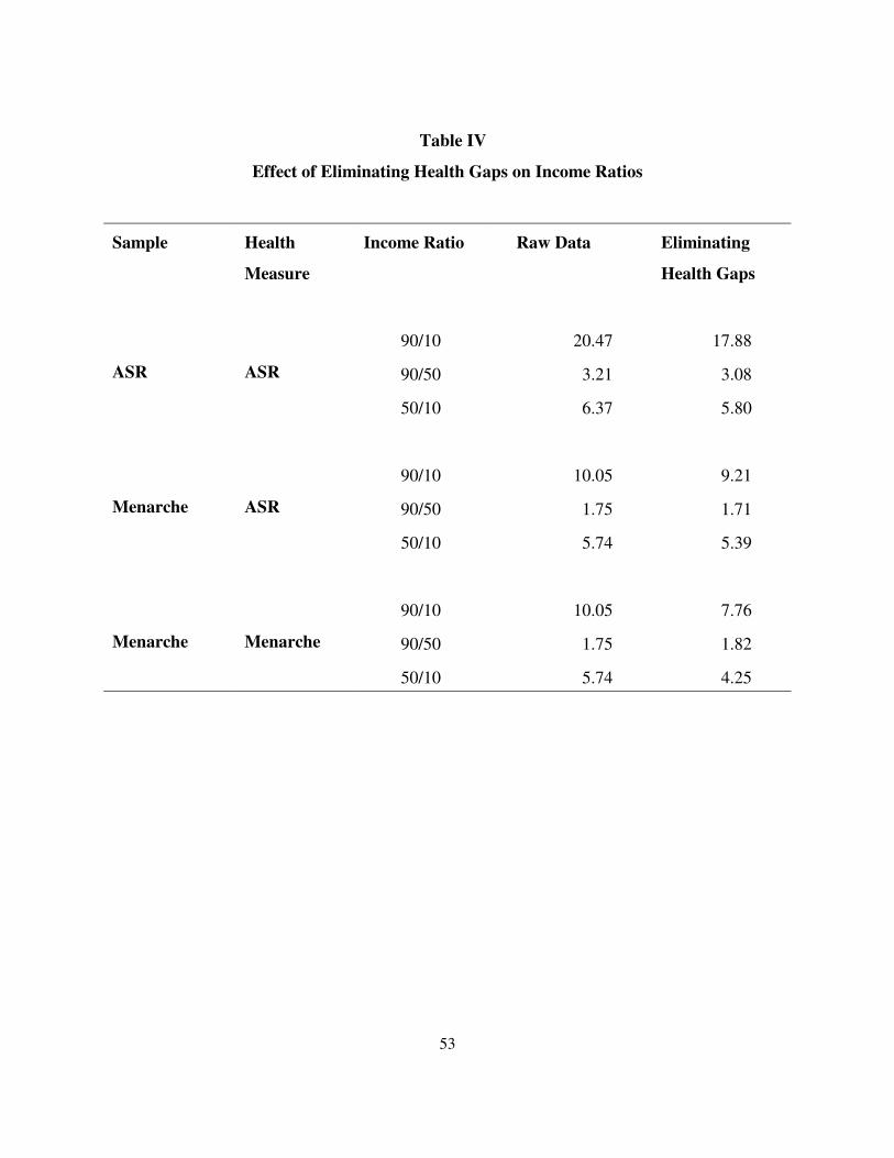
53
Table IV
Effect of Eliminating Health Gaps on Income Ratios
Sample Health
Measure
Income Ratio Raw Data Eliminating
Health Gaps
ASR ASR
90/10 20.47 17.88
90/50 3.21 3.08
50/10 6.37 5.80
Menarche ASR
90/10 10.05 9.21
90/50 1.75 1.71
50/10 5.74 5.39
Menarche Menarche
90/10 10.05 7.76
90/50 1.75 1.82
50/10 5.74 4.25

Figure IGDP per Worker vs. Adult Survival Rate
0.2
0.3
0.4
0.5
0.6
0.7
0.8
0.9
1
100 1000 10000 100000
GDP per Worker (1996)
Adu
lt Su
rviv
al R
ate
for M
ales
(19
99)
Botswana
South Africa
Zimbabwe
Guinea
Cote d'Ivore
Zambia
Central Afr. Rep.Rwanda
Uganda
Papua New Guinea

Figure II Adut Survival Rate
0.56
0.61
0.66
0.71
0.76
0.81
0.86
1960 1970 1980 1990 2000
Year
Mea
n A
SR
-0.1
-0.05
0
0.05
0.1
0.15
0.2
Stan
dard
Dev
iatio
n of
ASR
Mean ASR (left scale)
Standard Deviationof ASR (right scale)

Figure III
Age of Menarche vs. GDP per Worker
12
12.5
13
13.5
14
14.5
15
15.5
16
1000 10000 100000
GDP per Worker in 1995
Ag
e o
f M
en
arc
he
Nigeria
Haiti
Papua New Guinea
Mozambique
United States
Italy
Ireland
Nicaragua
Algeria
Thailand
Kenya
Zambia
Portugal
Norway
Malaysia

Figure IVData on Height and Adult Survival
400
450
500
550
600
650
700
750
800
850
900
162 164 166 168 170 172 174 176 178 180 182
height (cm)
Adu
lt Su
rviv
al R
ate
(per
thou
sand
)
DenmarkFranceItalyJapanS. KoreaNetherlandsSpainSwedenUKUSA

Figure VThe Effect of Eliminating Health Gaps Among Countries
0
0.02
0.04
0.06
0.08
0.1
0.12
0.14
0.16
0.18
0.2
1960 1970 1980 1990 2000
Year
Reduction in theVariance of ln(GDP/Worker)
Reduction in the 90/10 income ratio
Reduction in the 50/10 income ratio
Reduction in the 90/50 income ratio


![Counterparts[1] jose guzman](https://img.dokumen.tips/doc/110x75/558d536fd8b42a96338b462e/counterparts1-jose-guzman.jpg)


