University of Kentucky University of Kentucky

UKnowledge UKnowledge

Theses and Dissertations--Statistics Statistics

2018

ACCOUNTING FOR MATCHING UNCERTAINTY IN ACCOUNTING FOR MATCHING UNCERTAINTY IN

PHOTOGRAPHIC IDENTIFICATION STUDIES OF WILD ANIMALS PHOTOGRAPHIC IDENTIFICATION STUDIES OF WILD ANIMALS

Amanda R. Ellis University of Kentucky, arelli4@uky.edu Digital Object Identifier: https://doi.org/10.13023/ETD.2018.026

Right click to open a feedback form in a new tab to let us know how this document benefits you. Right click to open a feedback form in a new tab to let us know how this document benefits you.

Recommended Citation Recommended Citation Ellis, Amanda R., "ACCOUNTING FOR MATCHING UNCERTAINTY IN PHOTOGRAPHIC IDENTIFICATION STUDIES OF WILD ANIMALS" (2018). Theses and Dissertations--Statistics. 31. https://uknowledge.uky.edu/statistics_etds/31

This Doctoral Dissertation is brought to you for free and open access by the Statistics at UKnowledge. It has been accepted for inclusion in Theses and Dissertations--Statistics by an authorized administrator of UKnowledge. For more information, please contact UKnowledge@lsv.uky.edu.

STUDENT AGREEMENT: STUDENT AGREEMENT:

I represent that my thesis or dissertation and abstract are my original work. Proper attribution

has been given to all outside sources. I understand that I am solely responsible for obtaining

any needed copyright permissions. I have obtained needed written permission statement(s)

from the owner(s) of each third-party copyrighted matter to be included in my work, allowing

electronic distribution (if such use is not permitted by the fair use doctrine) which will be

submitted to UKnowledge as Additional File.

I hereby grant to The University of Kentucky and its agents the irrevocable, non-exclusive, and

royalty-free license to archive and make accessible my work in whole or in part in all forms of

media, now or hereafter known. I agree that the document mentioned above may be made

available immediately for worldwide access unless an embargo applies.

I retain all other ownership rights to the copyright of my work. I also retain the right to use in

future works (such as articles or books) all or part of my work. I understand that I am free to

register the copyright to my work.

REVIEW, APPROVAL AND ACCEPTANCE REVIEW, APPROVAL AND ACCEPTANCE

The document mentioned above has been reviewed and accepted by the student’s advisor, on

behalf of the advisory committee, and by the Director of Graduate Studies (DGS), on behalf of

the program; we verify that this is the final, approved version of the student’s thesis including all

changes required by the advisory committee. The undersigned agree to abide by the statements

above.

Amanda R. Ellis, Student

Dr. Simon Bonner, Major Professor

Dr. Constance L. Wood, Director of Graduate Studies

ACCOUNTING FOR MATCHING UNCERTAINTY IN PHOTOGRAPHIC IDENTIFICATIONSTUDIES OF WILD ANIMALS

DISSERTATION

A dissertation submitted in partial fulfillment of therequirements for the degree of Doctor of Philosophy in the

College of Arts and Sciencesat the University of Kentucky

By

Amanda R. Ellis

Lexington, Kentucky

Co-Directors: Dr. Simon Bonner, Professor of Statistics

and Dr. Richard Charnigo, Professor of Statistics

Lexington, Kentucky

Copyright c© Amanda R. Ellis 2018

ABSTRACT OF DISSERTATION

ACCOUNTING FOR MATCHING UNCERTAINTY IN PHOTOGRAPHIC IDENTIFICATIONSTUDIES OF WILD ANIMALS

I consider statistical modelling of data gathered by photographic identification in mark-recapturestudies and propose a new method that incorporates the inherent uncertainty of photographic iden-tification in the estimation of abundance, survival and recruitment. A hierarchical model is proposedwhich accepts scores assigned to pairs of photographs by pattern recognition algorithms as data andallows for uncertainty in matching photographs based on these scores. The new models incorporatelatent capture histories that are treated as unknown random variables informed by the data, con-trasting past models having the capture histories being fixed. The methods properly account foruncertainty in the matching process and avoid the need for researchers to confirm matches visually,which may be a time consuming and error prone process.

Through simulation and application to data obtained from a photographic identification studyof whale sharks I show that the proposed method produces estimates that are similar to when thetrue matching nature of the photographic pairs is known. I then extend the method to incorporateauxiliary information to predetermine matches and non-matches between pairs of photographs inorder to reduce computation time when fitting the model. Additionally, methods previously appliedto record linkage problems in survey statistics are borrowed to predetermine matches and non-matches based on scores that are deemed extreme. I fit the new models in the Bayesian paradigmvia Markov Chain Monte Carlo and custom code that is available by request.

KEYWORDS: Mark-Recapture, Photographic Identification, Bayesian Analysis, HierarchicalModel

AMANDA R. ELLISStudent’s Signature

DECEMBER 11, 2017

Date

ACCOUNTING FOR MATCHING UNCERTAINTY IN PHOTOGRAPHIC IDENTIFICATIONSTUDIES OF WILD ANIMALS

By

Amanda R. Ellis

SIMON BONNERCo-Director of Dissertation

RICHARD CHARNIGOCo-Director of Dissertation

CONSTANCE L. WOODDirector of Graduate Studies

DECEMBER 11, 2017

Date

To the one and only Barry “Bartholomew” Farmer. Without your love and support I neverwould have made it.

ACKNOWLEDGEMENTS

I would like to sincerely thank all of the wonderful teachers I have had throughout my graduatecareer. Without your patience and guidance I would not be where I am today. A special thankgoes to Dr. Bonner for managing to be a wonderful adviser despite being located in two differentcountries.

iii

Table of Contents

Acknowledgements . . . . . . . . . . . . . . . . . . . . . . . . . . . . . . . . . . . . . . . iii

List of Tables . . . . . . . . . . . . . . . . . . . . . . . . . . . . . . . . . . . . . . . . . . vi

List of Figures . . . . . . . . . . . . . . . . . . . . . . . . . . . . . . . . . . . . . . . . . . vii

1 Introduction . . . . . . . . . . . . . . . . . . . . . . . . . . . . . . . . . . . . . . . . . 11.1 Mark-Recapture Studies . . . . . . . . . . . . . . . . . . . . . . . . . . . . . . . . . . 1

1.1.1 Citizen Scientist Role in Mark-Recapture Studies . . . . . . . . . . . . . . . . 21.2 Mark-Recapture Models . . . . . . . . . . . . . . . . . . . . . . . . . . . . . . . . . . 3

1.2.1 Closed Population: Estimation of Abundance . . . . . . . . . . . . . . . . . . 51.2.2 Open Population: Estimation of Both Abundance and Recruitment/Survival 61.2.3 Open Population: Estimation of Only Recruitment/Survival . . . . . . . . . . 8

1.3 Estimation of Parameters with Markov Chain Monte Carlo . . . . . . . . . . . . . . 81.3.1 Directed Acyclic Graphs . . . . . . . . . . . . . . . . . . . . . . . . . . . . . . 91.3.2 Markov Chain Monte Carlo . . . . . . . . . . . . . . . . . . . . . . . . . . . . 10

1.4 Photo Identification . . . . . . . . . . . . . . . . . . . . . . . . . . . . . . . . . . . . 131.4.1 Incorporation of Pattern Recognition in Photo Identification . . . . . . . . . 13

1.5 Error in Identification . . . . . . . . . . . . . . . . . . . . . . . . . . . . . . . . . . . 161.6 Error in Photo Identification . . . . . . . . . . . . . . . . . . . . . . . . . . . . . . . 18

1.6.1 Ad hoc Methods . . . . . . . . . . . . . . . . . . . . . . . . . . . . . . . . . . 191.6.2 Frequentist Methods . . . . . . . . . . . . . . . . . . . . . . . . . . . . . . . . 191.6.3 Bayesian Methods . . . . . . . . . . . . . . . . . . . . . . . . . . . . . . . . . 20

1.7 Conclusion . . . . . . . . . . . . . . . . . . . . . . . . . . . . . . . . . . . . . . . . . 20

2 Modeling the Uncertainty of Photographic Identification . . . . . . . . . . . . . . 212.1 Introduction . . . . . . . . . . . . . . . . . . . . . . . . . . . . . . . . . . . . . . . . . 212.2 Methods . . . . . . . . . . . . . . . . . . . . . . . . . . . . . . . . . . . . . . . . . . . 22

2.2.1 Model . . . . . . . . . . . . . . . . . . . . . . . . . . . . . . . . . . . . . . . . 222.2.2 Inference . . . . . . . . . . . . . . . . . . . . . . . . . . . . . . . . . . . . . . 28

2.3 Application . . . . . . . . . . . . . . . . . . . . . . . . . . . . . . . . . . . . . . . . . 312.3.1 Data . . . . . . . . . . . . . . . . . . . . . . . . . . . . . . . . . . . . . . . . . 312.3.2 Model . . . . . . . . . . . . . . . . . . . . . . . . . . . . . . . . . . . . . . . . 352.3.3 Inference for the JS Model . . . . . . . . . . . . . . . . . . . . . . . . . . . . . 382.3.4 Sampler for JS model . . . . . . . . . . . . . . . . . . . . . . . . . . . . . . . 382.3.5 Initial Value for X . . . . . . . . . . . . . . . . . . . . . . . . . . . . . . . . . 392.3.6 MCMC Sampling . . . . . . . . . . . . . . . . . . . . . . . . . . . . . . . . . . 402.3.7 Updates for Mixing . . . . . . . . . . . . . . . . . . . . . . . . . . . . . . . . . 432.3.8 Need for Reversible Jump MCMC . . . . . . . . . . . . . . . . . . . . . . . . 45

2.4 Results . . . . . . . . . . . . . . . . . . . . . . . . . . . . . . . . . . . . . . . . . . . . 472.4.1 Simulated Data . . . . . . . . . . . . . . . . . . . . . . . . . . . . . . . . . . . 472.4.2 Whale Shark Data Set . . . . . . . . . . . . . . . . . . . . . . . . . . . . . . . 49

2.5 Discussion . . . . . . . . . . . . . . . . . . . . . . . . . . . . . . . . . . . . . . . . . . 52

iv

3 Incorporation of Auxiliary Data and Record Linkage Methods to Improve Com-putational Efficiency . . . . . . . . . . . . . . . . . . . . . . . . . . . . . . . . . . . . 553.1 Introduction . . . . . . . . . . . . . . . . . . . . . . . . . . . . . . . . . . . . . . . . . 55

3.1.1 Photographic Identification in a Record Linkage Framework . . . . . . . . . 553.2 Methods . . . . . . . . . . . . . . . . . . . . . . . . . . . . . . . . . . . . . . . . . . . 58

3.2.1 Restricting the Sample Space of C(X) . . . . . . . . . . . . . . . . . . . . . . 583.2.2 Fixing Elements of C(X) with Auxiliary Information . . . . . . . . . . . . . . 653.2.3 Application of Record Linkage Type Rule to Fix Elements of C(X) . . . . . 663.2.4 MCMC Sampling . . . . . . . . . . . . . . . . . . . . . . . . . . . . . . . . . . 863.2.5 Adding or Deleting an Individual with Dependencies . . . . . . . . . . . . . . 86

3.3 Application . . . . . . . . . . . . . . . . . . . . . . . . . . . . . . . . . . . . . . . . . 883.3.1 Simulated Data . . . . . . . . . . . . . . . . . . . . . . . . . . . . . . . . . . . 883.3.2 Whale Shark Data Set . . . . . . . . . . . . . . . . . . . . . . . . . . . . . . . 90

3.4 Discussion . . . . . . . . . . . . . . . . . . . . . . . . . . . . . . . . . . . . . . . . . . 95

4 Conclusion . . . . . . . . . . . . . . . . . . . . . . . . . . . . . . . . . . . . . . . . . . 974.1 Introduction . . . . . . . . . . . . . . . . . . . . . . . . . . . . . . . . . . . . . . . . . 974.2 Computational Improvement . . . . . . . . . . . . . . . . . . . . . . . . . . . . . . . 984.3 Extension to Other Underlying Mark-Recapture Models and Data Sets . . . . . . . . 994.4 Further Exploration of Citizen Scientist Data . . . . . . . . . . . . . . . . . . . . . . 100

4.4.1 Lack Experimental Design on Estimates of Abundance and Capture Probability1004.4.2 Choice of Primary Occasions in Open Robust Design . . . . . . . . . . . . . . 101

A Appendix . . . . . . . . . . . . . . . . . . . . . . . . . . . . . . . . . . . . . . . . . . .102A.1 Cardinality of CY With and Without Restrictions . . . . . . . . . . . . . . . . . . . . 102

A.1.1 Cardinality of CY with No Restrictions . . . . . . . . . . . . . . . . . . . . . . 103A.1.2 Cardinality of CY when Non-Matches are Predetermined . . . . . . . . . . . . 103A.1.3 Cardinality of CY when Matches are Predetermined . . . . . . . . . . . . . . 104A.1.4 Cardinality of CY when Non-Matches and Matches are Predetermined . . . . 106

Bibliography . . . . . . . . . . . . . . . . . . . . . . . . . . . . . . . . . . . . . . . . . . .109

Vita . . . . . . . . . . . . . . . . . . . . . . . . . . . . . . . . . . . . . . . . . . . . . . . .114

v

List of Tables

2.1 Model Notation . . . . . . . . . . . . . . . . . . . . . . . . . . . . . . . . . . . . . . . 222.2 Additional Notation Needed for JS Model . . . . . . . . . . . . . . . . . . . . . . . . 382.3 Results from Simulated Data N with False Matches and Non-Matches . . . . . . . . 492.4 Results from Simulated Data N with Score Based Mark-Recapture Model . . . . . . 492.5 Results from Simulated Data φ with Score Based Mark-Recapture model . . . . . . 502.6 Results from Simulated Data p with Score Based Mark-Recapture model . . . . . . 50

3.1 Results from Simulated Data N . . . . . . . . . . . . . . . . . . . . . . . . . . . . . . 893.2 Comparison of Computational Time for the Score Based Mark-Recapture Model and

Fast Score Based Mark-Recapture Model . . . . . . . . . . . . . . . . . . . . . . . . 90

vi

List of Figures

1.1 Growth of Reported Sightings of Whale Sharks Documented by Citizen Scientist . . 31.2 Directed Acyclic Graph (DAG) Representation of Model Mt. Where N is the total

population size and p is the vector of capture probabilities. . . . . . . . . . . . . . . 91.3 Directed Acyclic graph (DAG) Representation of the CMSA Formulation of the JS

Model. Where N is the total population size, β is the vector of birth probabilities,b is the latent birth vector, d is the latent death vector, φ is the vector of survivalprobabilities, p is the vector of capture probabilities andW obs is the observed capturehistory matrix. . . . . . . . . . . . . . . . . . . . . . . . . . . . . . . . . . . . . . . . 10

1.4 Sketch of Basic Pattern Comparison . . . . . . . . . . . . . . . . . . . . . . . . . . . 15

2.1 Directed Acyclic Graph (DAG) Representation of the Proposed Hierarchical Modelwith Generic Underlying Mark-Recapture Model. . . . . . . . . . . . . . . . . . . . . 29

2.2 Directed Acyclic Graph (DAG) Representation of the Proposed Hierarchical Modelwith Model Mt. . . . . . . . . . . . . . . . . . . . . . . . . . . . . . . . . . . . . . . . 30

2.3 Side View of Whale Shark . . . . . . . . . . . . . . . . . . . . . . . . . . . . . . . . . 322.4 Comparison of the Density of Log Match vs Non-Match Scores. . . . . . . . . . . . . 332.5 Number of Encounters per Year . . . . . . . . . . . . . . . . . . . . . . . . . . . . . . 352.6 DAG of Score Based Mark-Recapture Model with CMSA Formulation . . . . . . . . 372.7 Initial Value Plot . . . . . . . . . . . . . . . . . . . . . . . . . . . . . . . . . . . . . . 392.8 Comparison of the Estimates of φ . . . . . . . . . . . . . . . . . . . . . . . . . . . . 512.9 Comparison of the Posterior Distributions of p . . . . . . . . . . . . . . . . . . . . . 52

3.1 Fitted Density of Observed Scores . . . . . . . . . . . . . . . . . . . . . . . . . . . . 673.2 Beta Mixture with Identification of Match Scores . . . . . . . . . . . . . . . . . . . . 683.3 Beta Mixture with Identification of Non-Match Scores . . . . . . . . . . . . . . . . . 813.4 Comparison of the Estimates of φ for the CMSA Model, Score Based Mark-Recapture

Model, and the Fast Score Based Mark-Recapture Model . . . . . . . . . . . . . . . 933.5 Comparison of the Posterior Distributions of p for the CMSA Model, Score Based

Mark-Recapture model, and the Fast Score Based Mark-Recapture Model . . . . . . 943.6 Comparison of the Posterior Distributions of N for the CMSA Model, Score Based

Mark-Recapture model, and the Fast Score Based Mark-Recapture model . . . . . . 95

4.1 Directed Acyclic Graph (DAG) Representation of a Model for the Estimation of Abun-dance Not Incorporating an Underlying Mark-Recapture Model . . . . . . . . . . . . 99

vii

Chapter 1

Introduction

The American photographer Bernice Abbott once stated “Photography helps people see” (Shepard,

1989). At the time she was referencing photography’s ability to teach an artist the importance of

the relationship between background and foreground in an image. Photography can help researchers

see in a different way. Researchers often are interested in learning about animal populations, but

examining the entire population is an impossible task. Photography of a subset of a population

of animals allows researchers to ”see” or make inference about an entire population. My work

focuses on methods that utilize photographs of animals to gain inference. In what follows I provide;

background information that describes the studies conducted by researchers, the role of photographs

as data, and statistical tools that help researchers gain inference from those studies.

1.1 Mark-Recapture Studies

According to Amstrup et al. (2010), mark-recapture studies have been implemented since the early

1800s and are a valuable tool that aid biologists in gaining information about a population of

animals or people. Researchers begin a mark-recapture study by determining a set number of capture

occasions on which they plan to capture animals. How the animals are captured varies across studies.

Some studies physically capture the animals with traps like mesh cages or nets (Wilson et al., 2007).

On the first occasion, researchers capture an initial group of animals that are marked, and released

back into the population. Then on the second capture occasion, researchers collect a second group

of animals containing both marked and unmarked individuals. Those individuals without marks are

then marked and all animals are released back into the population. This process continues until the

end of the study.

Traditional mark-recapture studies relied on man-made methods to mark the animals in the

study. Examples of man-made marks include the insertion of pit tags into snakes (Keck, 1994), bands

on birds (Seber, 1970) and digit clipping in amphibians (McCarthy and Parris, 2004). Researchers

have studied the implementation of man-made markings and the potential impact on estimates of

parameters of interest (Paulissen and Meyer, 2000; Bortolotti, 1994). Other studies incorporate

non-invasive capture and marking techniques such as collecting DNA left behind by animals (Mowat

and Strobeck, 2000) or taking photographs of unique markings (Trolle and Kery, 2003), which is the

focus of my work.

1

1.1.1 Citizen Scientist Role in Mark-Recapture Studies

Historically the data for mark-recapture studies came from studies that were designed and conducted

by researchers. Before the start of a study, researchers would determine the number of capture

occasions and the physical area where they would like to investigate the animal. Then the researcher

would go out in the field, capture the animals and record the data. As an example Petersen (1896)

describes a study in which researchers traveled along the Limfjord to the German Sea capturing

and marking plaice (a commercially valuable flat fish) by placing holes in the fins of the fish. The

location and time of the study were determined before the researchers began collecting the fish.

Recent years have seen an influx of data not derived from researchers collecting data from the

field but rather from citizen scientist. Silvertown (2009, p 1) defines citizen scientist as: “A volunteer

who collects and/or processes data as part of a scientific inquiry” and goes to say that “Projects

that involve citizen scientists are burgeoning, particularly in ecology and the environmental sci-

ences, although the roots of citizen science go back to the very beginnings of modern science itself.”

Researchers are beginning to see reports from citizen scientist as a significant tool for gathering

information that can be considered as data in mark-recapture studies. Cohn (2008, p. 2) looks at

the collaboration between citizen scientists and traditional scientists, and states: “Collaborations

between scientists and volunteers have the potential to broaden the scope of research and enhance

the ability to collect scientific data. Interested members of the public may contribute valuable

information as they learn about wildlife in their local communities.”

A direct example of the contribution of citizen scientists is in the study of whale sharks (Rhincodon

typus) in the northern ecotourism zone of the Nigaloo Marine Park near Exmouth on the North West

Cape of Australia (21◦ 55’59S 114◦ 7’41E). Boats and spotter planes travel daily during the annual

whale shark aggregation (March to July) to locate the animals. After the animals are spotted

tourists travel to where the whale sharks are located and later upload photos of the animals to

whaleshark.org, a website dedicated to cataloging and storing images of whale sharks. Complete

details are available in Holmberg et al. (2009). To date over 5,000 citizen scientist have contributed to

the website. Figure 1.1 shows the growth in the number of sightings by citizen scientist over recent

years. Researchers are able to utilize the photographs, which depict unique naturally occurring

marks, of whale sharks uploaded by the citizen scientist to determine captures of the whale sharks.

2

Figure 1.1: Growth of Reported Sightings of Whale Sharks Documented by Citizen Scientist

An obvious but important distinction of considering the photographs uploaded by the citizen

scientist as captures is that the study did not have pre-determined capture occasions or physical

location for the photographs to be taken in. Citizen scientists upload photographs to the website,

after which researchers decide which photographs to consider based on the time and location they

are interested in. My work considers the photographs contributed by citizen scientist as captures but

has not explored how the lack of preemptive study design influences inference about the population

parameters.

1.2 Mark-Recapture Models

There are two basic types of mark-recapture models: open population and closed population models.

Closed population models assume the population is not changing through births, deaths, immigra-

tion or emigration and these models focus on estimating population size. Open population models

estimate survival or recruitment probabilities and may allow for immigration and emigration. The

ratio of marked versus unmarked animals at each occasion of the study gives information about

abundance. The re-sighting of individuals across occasions provides information about survival, re-

cruitment and capture probabilities. There are many extensions to these basic models. The data

for the models may be stored in an observed capture matrix, more information on the matrix will

be provided later. My work is applicable to both closed and open models and will include the full

capture history matrix discussed below.

3

To illustrate the observed capture history matrix consider five capture occasions. On the first

capture occasion, researchers capture a group of the animal of interest. The captured animals are

given unique marks and released back into the wild. On the second capture occasion, researchers

again capture a group of animals. This group will contain some marked and some non-marked

animals. On the second capture each non-marked animal is uniquely marked, and all the captured

animals are again released back into the wild. This process continues until the final capture occasion.

The full capture history matrix, W, reflects when each animal in the population was captured. The

matrix is comprised of 0’s, and 1’s where a one denotes the animal was captured and a zero denotes

that the animal was not captured. Each column in the capture history matrix represents a capture

occasion and each row represents the history of a unique animal.

Here I note the distinction between the observed capture history matrix and the true latent

capture history matrix. The observed capture occasion matrix only contains information about

those individuals seen during the study. I will denote the observed capture history matrix Wobs.

Since Wobs only contains information about observed animals, every row of Wobs contains at least

one 1. There will be some animals in the population which are never observed, having a capture

history of all zeros and are not included in Wobs. The true latent capture occasion matrix, W, will

contain some rows of all zeros representing those individuals that are never seen and is never fully

observed. Further note that Wobs and W will have different dimensions: if N is the total population

size and n is the number of individuals ever captured then Wobs has dimension n × T and W has

dimension N × T , where T is the number of capture occasions.

Suppose that over the 5 capture occasions 9 individuals were observed during the study. A

potential realization of Wobs is given below.

Wobs =

1 0 1 0 0

1 0 1 0 0

0 1 0 0 0

1 1 1 0 1

0 1 0 1 0

0 1 1 0 0

0 0 1 0 0

1 0 1 0 0

0 1 0 0 0

4

The first row of Wobs would represent that a single animal was caught on occasions 1 and 3 but not

on occasions 2, 4 and 5. It should also be noted that the ordering of the rows of Wobs is arbitrary.

Further notice that each row contains at least one 1 since Wobs only represents animals that were

observed. The latent matrix W would look similar but would additionally have rows of all zeros

representing those animals that were never captured.

In upcoming sections, I will briefly introduce some of the more common mark-recapture models.

I summarize the models utilizing three categories: models that estimate abundance, models that

estimate recruitment/survival and models that estimate both abundance and recruitment/survival.

In each category I will present models of historical importance and how those models evolved into

models referenced in later chapters. In Chapter 2, I will introduce a framework that incorporates an

underlying mark-recapture model into a larger hierarchical model that considers information from

the comparison of photographs as data.

1.2.1 Closed Population: Estimation of Abundance

Previously discussed was the work of Petersen (1896), which is one of the earliest examples of closed

population models for animals, the primary goal of the paper was the estimation of abundance of

European plaice. The estimation was accomplished by implementing one of the earliest methods of

estimating abundance using mark-recapture methods. The paper considered a two occasion study

where the ratio of marked and unmarked animals in the second occasion produced what is known

as the Lincoln-Petersen Estimator. This estimator of abundance is one of the most simplistic and

has restrictive model assumptions such as equal probability of capture on each of the 2 capture

occasion and the population be closed. The estimation of abundance from closed populations was

further discussed and developed in the work of Otis et al. (1978). This paper considers a study

with T capture occasions and defines closed population models in which the probability of capture is

constant over time, varies with time or varies by individual. Some of the models introduced are M0,

Mt, Mb and Mh, which are some of the most well known closed population models. The subscript

on each of the models denotes the dependency of the capture probability. In model M0 there is

no variation of the capture probability across individuals or time, in Mt the capture probability

depends on the time of capture, in model Mb the capture probability is dependent on a behavior

response to being previously captured, and in model Mh the capture probabilities are heterogeneous

across individuals.

In Chapter 2 I will incorporate model Mt into the proposed framework. Model Mt is a closed

population model with constant probability of capture for all individuals on a given occasion. Let N

5

denote the total population size and pt denote the probability of capture on occasion t, t = 1, . . . , T

where T is the total number of capture occasions. Borrowing notation from Link and Barker (2009)

the complete data likelihood (CDL) for the model is:

[W|N,p] ∝(N

u.

) T∏t=1

pntt (1− pt)N−nt (1.1)

where ut represents the number of unmarked animals in sample t and u. =∑Tt=1 ut. More informa-

tion on fitting the model and details on the distributions that form the CDL can be found in Link

and Barker (2009, p 204). This information will be needed in Chapter 2 to define the CDL for an

extended hierarchical model.

1.2.2 Open Population: Estimation of Both Abundance and Recruitment/Survival

Both Jolly (1965) and Seber (1965) introduced a model that estimates abundance and recruit-

ment/survival of animals for open populations known as the Jolly-Seber (JS) model. The model

requires that a single population be specified, meaning that there is a well-defined area in which the

members of the population are free to mix within. Implementing the model, researchers can make

inference about; year specific capture probabilities, recruitment probabilities and abundance. Infer-

ence can also be made about apparent survival, which is defined to be when death and emigration

cannot be distinguished from one another.

Crosbie and Manly (1985) provided an important variation of the JS model that allows for

alternative assumptions for survival probabilities, ingress times and capture probabilities. A general

multinomial modeling approach is presented and allows for survival probabilities to be time-specific,

age specific or constant. Additionally, the paper allows capture probabilities to be time specific or

constant. The results of this model are similar to the JS model when animals are assumed to enter

the population in batches before sample times, but differences do occur if the animals can enter at

any time between samples. Pollock et al. (1990) gives an overview of mark-recapture models and

introduced restricted versions of the work presented in Jolly (1965); Seber (1965). The restricted

versions include a death only model, birth only model and constant survival and capture models.

The death only model was originally developed to account for no loss on capture by Darroch (1959)

and was further developed by Jolly (1965). I provide more details on this model in section 1.2.3.

In addition to the restricted models, generalizations of the JS model are provided in Pollock et al.

(1990) including a temporary trap response model and a cohort model.

6

Schwarz and Arnason (1996) further extended the JS model by introducing what is known as

the POPAN formulation. This formulation models births with a multinomial distribution from a

super-population. The super-population consist of all animals ever available for capture during the

study. In some cases, defining the super-population for a population of interest can be difficult.

By utilizing the multinomial distribution, the work is able simplify numerical optimization of the

likelihood and are easily able to impose constraints on the model parameters. This model is also

known as the CMSA formulation and is discussed in Link and Barker (2005). An advantage of this

formulation is that it is amenable to hierarchical extension and can easily incorporate covariates.

In Chapter 2 I will incorporate the CMSA formulation of the JS model into the proposed frame-

work. Let N denote the number of animals ever available for capture during the study. I denote

the probability of capture on occasion t as pt where t = 1, . . . , T and φt as the probability that an

individual alive and in the population at time t, is alive and in the population at time t+ 1. Further

let b be the latent birth vector of length N , where bi=t denotes the individual was born between

times t − 1 and t. Similarly let d be the latent death vector of length N , where di=t denotes the

individual died between times t and t+ 1. Borrowing notation from Link and Barker (2009, p 255)

the CDL for the model is:

[W,b,d|N,β,p,φ] ∝ [W|p, N,b,d][d|φ,b, N ][b|β, N ] (1.2)

The term [W|p, N,b,d] is similar to the CDL for model Mt previously discussed with the only

difference being that animals have probability of capture equal to zero prior to being born and after

death. The term [d|φ,b, N ] models the deaths of the animals where

[d|φ,b, N ] ∝N∏i=1

[di|φ,b]. (1.3)

For each animal, [di|φ,b] is a categorical distribution with sample space k, .., T and parameter vector

φ, where k is the occasion on which the animal is born and φ is the probability of survival. Similarly

the term [b|β, N ] models the births of the animals where

[b|β, N ] ∝N∏i=1

[bi|β]. (1.4)

For each animal [bi|β] is a categorical distribution with sample space 1, .., T and parameter vector

β, where βt is the probability that an individual ever available for capture enters between times t

7

and t+ 1.

1.2.3 Open Population: Estimation of Only Recruitment/Survival

Many researchers that conduct mark-recapture studies are only interested in estimating survival.

Cormack (1964) was a precursor to the work presented in Jolly (1965) and Seber (1965) and provides

a simplified method to only estimate survival and capture by conditioning on the first capture

occasion. The model is widely known as the Cormack-Jolly-Seber (CJS) model and is one of the

most commonly employed mark-recapture models. Link and Barker (2009, p 98) states: “The

Cormack-Jolly-Seber (CJS) model is of enormous importance in wildlife studies; its development

by Cormack (1964) and later extensions by Jolly (1965) and Seber (1965) are important milestones

in the advancement of statistical methodology for estimating demographic parameters.” One of the

advantages to this model is it does not require the researcher to define a super population. An

important extension to this model was developed in Lebreton et al. (1992). The paper discusses

model building and selection for open population models. Additionally, the paper considers the

effects of time, age, and categorical variables such as gender on survival and capture rates, as well as

interactions between such effects. I do not explicitly incorporate the CJS model into my framework,

but the methods I present in later chapters could easily include this valuable model. In the next

section I discuss some necessary background information on how inference about the parameters of

the mark-recapture models may be obtained.

1.3 Estimation of Parameters with Markov Chain Monte Carlo

Early estimation of the parameters in mark-recapture models implemented frequentist methodology.

As models became more complex and hierarchical models were developed researchers began to in-

corporate Bayesian methods to make inference about the population parameters. In later chapters,

I will present complex hierarchical models and will implement Bayesian methodology to make infer-

ence. In this section, I look at two useful tools commonly employed by Bayesian methodology. First

I will discuss the application of directed acyclic graphs to summarize hierarchical models. After

which I will briefly discuss Markov Chain Monte Carlo with a focus on the sampling methods I will

reference in later chapters.

8

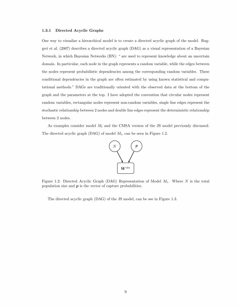
1.3.1 Directed Acyclic Graphs

One way to visualize a hierarchical model is to create a directed acyclic graph of the model. Rug-

geri et al. (2007) describes a directed acyclic graph (DAG) as a visual representation of a Bayesian

Network, in which Bayesian Networks (BN): “ are used to represent knowledge about an uncertain

domain. In particular, each node in the graph represents a random variable, while the edges between

the nodes represent probabilistic dependencies among the corresponding random variables. These

conditional dependencies in the graph are often estimated by using known statistical and compu-

tational methods.” DAGs are traditionally oriented with the observed data at the bottom of the

graph and the parameters at the top. I have adopted the convention that circular nodes represent

random variables, rectangular nodes represent non-random variables, single line edges represent the

stochastic relationship between 2 nodes and double line edges represent the deterministic relationship

between 2 nodes.

As examples consider model Mt and the CMSA version of the JS model previously discussed.

The directed acyclic graph (DAG) of model Mt, can be seen in Figure 1.2.

N p

W obs

Figure 1.2: Directed Acyclic Graph (DAG) Representation of Model Mt. Where N is the totalpopulation size and p is the vector of capture probabilities.

The directed acyclic graph (DAG) of the JS model, can be see in Figure 1.3.

9

N β

b

d

φ

p

W obs

Figure 1.3: Directed Acyclic graph (DAG) Representation of the CMSA Formulation of the JSModel. Where N is the total population size, β is the vector of birth probabilities, b is the latentbirth vector, d is the latent death vector, φ is the vector of survival probabilities, p is the vector ofcapture probabilities and W obs is the observed capture history matrix.

Notice in both figures the observed capture history matrix, Wobs, is located at the bottom of the

graph. The parameters and latent data are in the upper portions of the graph. These DAGs will be

beneficial in later chapters when describing and visualizing extended versions of the models.

1.3.2 Markov Chain Monte Carlo

When applying Bayesian methodology to make inference about a set of parameters researchers ideally

would like to achieve inference by identifying the posterior distribution of the parameters of interest.

The framework that I present in later chapters defines models that result in posterior distributions

that cannot be easily explored analytically. Markov Chain Monte Carlo (MCMC) gives researchers

a way to sample from the posterior distribution which is useful in situations when computing the

summary statistics from the posterior is difficult. There are many different types of samplers that

researchers often utilize. I will focus on two of the most common algorithms, which my work will

take advantage of, the Metropolis-Hastings algorithm and the Gibbs Sampler.

I begin by reviewing the Metropolis-Hastings algorithm that was first introduced by Hastings

(1970). The Metropolis-Hastings algorithm is the most general of sampling algorithms and serves

as a base for other sampling algorithms. It defines a way to obtain a random sample from any tar-

get distribution by first sampling from a known proposal distribution, then accepting the proposed

sample with probability comprised of both the proposed density and target density. Borrowing the

notation of Gelman et al. (2014), the algorithm is summarized in Algorithm 1.

One of the advantages of of the Metropolis-Hastings algorithm is that the algorithm may be per-

10

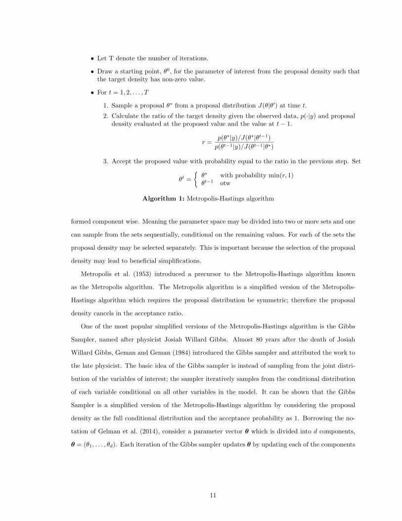
• Let T denote the number of iterations.

• Draw a starting point, θ0, for the parameter of interest from the proposal density such thatthe target density has non-zero value.

• For t = 1, 2, . . . , T

1. Sample a proposal θ∗ from a proposal distribution J(θ|θ′) at time t.

2. Calculate the ratio of the target density given the observed data, p(·|y) and proposaldensity evaluated at the proposed value and the value at t− 1.

r =p(θ∗|y)/J(θ∗|θt−1)

p(θt−1|y)/J(θt−1|θ∗)

3. Accept the proposed value with probability equal to the ratio in the previous step. Set

θt =

{θ∗ with probability min(r, 1)θt−1 otw

Algorithm 1: Metropolis-Hastings algorithm

formed component wise. Meaning the parameter space may be divided into two or more sets and one

can sample from the sets sequentially, conditional on the remaining values. For each of the sets the

proposal density may be selected separately. This is important because the selection of the proposal

density may lead to beneficial simplifications.

Metropolis et al. (1953) introduced a precursor to the Metropolis-Hastings algorithm known

as the Metropolis algorithm. The Metropolis algorithm is a simplified version of the Metropolis-

Hastings algorithm which requires the proposal distribution be symmetric; therefore the proposal

density cancels in the acceptance ratio.

One of the most popular simplified versions of the Metropolis-Hastings algorithm is the Gibbs

Sampler, named after physicist Josiah Willard Gibbs. Almost 80 years after the death of Josiah

Willard Gibbs, Geman and Geman (1984) introduced the Gibbs sampler and attributed the work to

the late physicist. The basic idea of the Gibbs sampler is instead of sampling from the joint distri-

bution of the variables of interest; the sampler iteratively samples from the conditional distribution

of each variable conditional on all other variables in the model. It can be shown that the Gibbs

Sampler is a simplified version of the Metropolis-Hastings algorithm by considering the proposal

density as the full conditional distribution and the acceptance probability as 1. Borrowing the no-

tation of Gelman et al. (2014), consider a parameter vector θ which is divided into d components,

θ = (θ1, . . . , θd). Each iteration of the Gibbs sampler updates θ by updating each of the components

11

of θ conditional on the other components and the data. Let,

p(θj |θt−1−j , y)

represent the distribution of θj given the other d−1 components of θ and the data, y. Each iteration

of the Gibbs sampler will cycle through j = 1, . . . , d and sample from the above distribution. The

Gibbs Sampler requires p(θj |θt−1−j , y) be in closed form and is a simplified version of the Metropolis-

Hastings algorithm. Often it is the case that the conditional distributions are not known in closed

form. Tierney (1994) suggests a mixture of the Gibbs Sampler and Metropolis-Hastings algorithm,

known as Metropolis-Hastings within Gibbs. The basic idea is to implement a Metropolis-Hastings

Step to accept/reject a proposed value when updating some of the components in an iteration

of a Gibbs Sampler. In later chapters when fitting a proposed model, I present a sampler that

incorporates both Gibbs and Metropolis-Hastings within Gibbs steps.

The methods I present in later chapters consider information from the photographs of unique

markings as data. The model that will be presented includes a latent variable that changes dimen-

sion. In cases like this Green (1995) suggest the application of Reversible Jump Markov Chain Monte

Carlo (RJMCMC). RJMCMC is often implemented when it is desirable to sample from potential

candidate models; for example, if choosing different regression models. For this reason RJMCMC al-

gorithms are often summarized in terms of sampling from potential models Mk, where k = 1, . . . ,K

and θk is the parameter set for model k with dimension dk (Gelman et al., 2014). In the case

of my work I am not sampling from potential models, but rather potential dimensions. For conve-

nience, in Algorithm 2 I summarize the RJMCMC algorithm borrowing the notation of Gelman et al.

(2014) which considers the case of choosing models but again this is the same as choosing dimension.

1. Starting with model Mk having parameter vector θk, (k, θk), propose a new model Mk∗ withprobability Jk,k∗ and generate an augmenting random variable u from proposal densityJ(u|k, k∗, θk).

2. Determine the proposed model’s parameters, (θk∗ , u∗) = gk,k∗(θk, u)

3. Define the ratio

r =p(y|θk∗ ,Mk∗)p(θk∗ |Mk∗)πk∗

p(y|θk,Mk)p(θk|Mk)πk

Jk∗,kJ(u∗|k∗, k, θk∗)Jk,k∗J(u|k, k∗, θk)

∣∣∣∣∇gk,k∗(θk, u)

∇(θk, u)

∣∣∣∣and accept the new model with probability min(r,1).

Algorithm 2: RJMCMC Algorithm

12

1.4 Photo Identification

Photo identification provides a low cost, non-invasive way to identify animals in mark-recapture

studies. This is especially beneficial when animals are hard to find or to capture (Cutler and Swann,

1999) and has been performed since the 1960s, (Guinet, 1988). Examples include studies of large

cats (Hiby et al., 2009) and large marine animals (Langtimm et al., 2004; Calambokidis et al., 1990).

Photo identification also provides a non-invasive method to identify animals that may be affected

by physical capture. Bansemer and Bennett (2008, p. 322) states: “Photographic identification

methodologies are therefore generally considered to be non-invasive, although the possibility remains

that the presence of photographers in proximity to the study-species may affect its behavior.” The

implementation of photo identification requires the animals possess a unique marking pattern that

can either be naturally occurring or caused from an external source. Examples of naturally occurring

marks include stripe patterns on tigers (Karanth and Nichols, 1998), while examples of marks caused

by external sources include scar patterns on Florida manatees (Kendall et al., 2004).

Due to advancements in technology the quality and availability of photo identification is becoming

more widely applied. Sarmento et al. (2010, p. 61) states the following: “The rapid expansion of

camera-trap surveys for elusive species has led to the widespread application of this technique,

as camera technology improved and equipment costs decreased.” In addition to more widespread

application of photo identification, the advancement in technology has also lead to increased size

of photographic catalogs. As an example whaleshark.org current host over 40,000 photographs.

(Holmberg, 2003)

1.4.1 Incorporation of Pattern Recognition in Photo Identification

Recent studies often collect large numbers of photographs that cannot be examined by eye alone.

When photo identification was first introduced researchers would only have a small pool of pho-

tographs to compare. Each of the photographs were visually compared by specially trained re-

searchers to determine if the same animal appeared in more than one photograph. Researchers have

started to run computer algorithms that rely on pattern recognition to help determine the matches.

There are several species that have been studied implementing algorithms to assist in the identifi-

cation process including: whale sharks (Arzoumanian et al., 2005), dolphins (Hillman et al., 2003),

sperm whales (Beekmans et al., 2005), polar bears (Anderson et al., 2010) and great white sharks

(Gubili et al., 2009). Algorithms assign each pair of photographs in a catalog a score, generally

high scores are considered a probable match while low scores are considered a probable non-match.

13

Trained researchers then confirm the matches.

In the 2005 paper An Astronomical Pattern-Matching Algorithm for Computer-Aided Identifica-

tion of Whale Sharks Rhincodon Typus, Arzoumanian et al. (2005) discusses how whale sharks can

be uniquely identified by photographs of naturally occurring spot patterns. Implementing a method

adapted from astronomy, the paper examines triangles that are formed from the spot patterns and

describes a method to identify unique photos. The photos are matched by identifying all triangles

formed by the spots on the animals, this is accomplished by comparing R (Ratio of long and short

side) and C (cosine at the vertex which connects the longest and shortest side) values. True matches

are distinguished from false matches by considering the possible triangles in each photo and compar-

ing pairwise the triangles with similar geometry. For each of the pairs a relative magnification factor

is computed. If the magnification factor is similar for all the pairs then the photographs are likely

to depict the same individual. Arzoumanian et al. (2005, p. 1003) describe Figure 1.4 as “A sketch

of the basic pattern-comparison process based on the formation of triangles from triplets of points.

Only subsets of all possible triangles are shown.” Problems with the method include image quality,

the angle at which the photograph was taken and spot pattern systematic, meaning the underlying

pattern of the spots. The paper claims reliability of match identification near 90% . Additional

computer algorithms have been developed to aid in photo identification. One such algorithm is

described in Crall et al. (2013), known as Hotspotter, is implemented by the group Image Based

Ecological Information System (IBEIS).

14

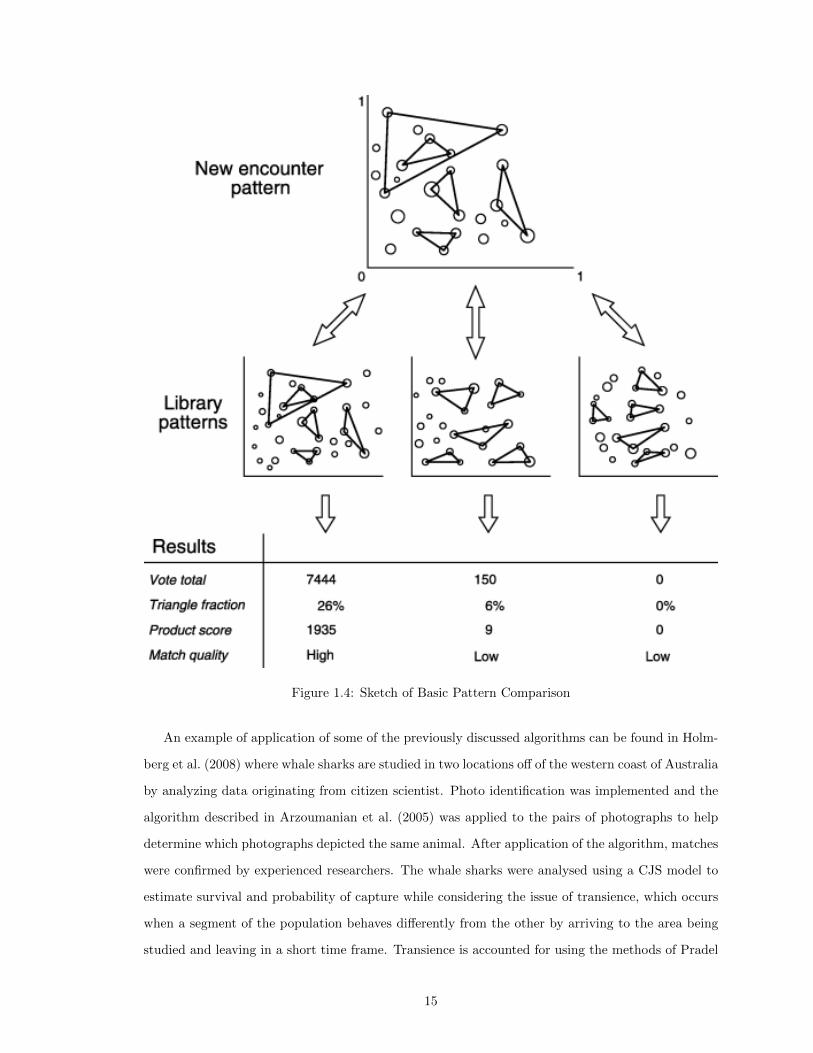
Figure 1.4: Sketch of Basic Pattern Comparison

An example of application of some of the previously discussed algorithms can be found in Holm-

berg et al. (2008) where whale sharks are studied in two locations off of the western coast of Australia

by analyzing data originating from citizen scientist. Photo identification was implemented and the

algorithm described in Arzoumanian et al. (2005) was applied to the pairs of photographs to help

determine which photographs depicted the same animal. After application of the algorithm, matches

were confirmed by experienced researchers. The whale sharks were analysed using a CJS model to

estimate survival and probability of capture while considering the issue of transience, which occurs

when a segment of the population behaves differently from the other by arriving to the area being

studied and leaving in a short time frame. Transience is accounted for using the methods of Pradel

15

et al. (1997). They found a site specific influence and opted to only consider data from the northern

region.

Holmberg et al. (2009) also evaluated the whale shark data by implementing computer algorithms

to aid in the matching of photographs. The paper differs from the previous work by fitting an open

robust model with length as a covariate. Two computer algorithms were employed to identify

matching pairs and a trained researcher confirmed. In addition to the pattern recognition algorithm

from Arzoumanian et al. (2005), the paper also compares the photographs with the algorithm defined

in Van Tienhoven et al. (2007).

1.5 Error in Identification

Mark-recapture studies require that animals be marked in some way. These marks can take the

form of natural marking or man made markings each having a risk of evolution of the marks, loss

of marks or misidentification. The majority of mark-recapture models assume that the markings

are non-evolving and are not lost over time. Researchers first considered error in identification of

animals due to tag loss, when an animal looses its tag and is recaptured researchers run the risk of

incorrectly identifying the animal as a new distinct animal instead of an animal that has already

been captured. Both Arnason and Mills (1981) and McDonald et al. (2003) discuss the bias and loss

of precision that can occur in the JS model when misidentification due to tag loss occurs. One of the

early solutions to the problem of misidentification due to tag loss over time was the introduction of

double tagging in studies. Robson and Regier (1966), Wetherall (1982) and Seber and Felton (1981)

all discuss double tagging in mark-recapture studies and how double tagging allows researchers to

estimate the chances of an animal loosing a tag which in turn allows researchers to address bias

in the parameter estimates caused by misidentification due to loss of tags. Cowen and Schwarz

(2006) considers the JS model and accounts for the bias that occurs in the parameter estimates

when marks are lost over time. Previous to the paper the issue of dealing with loss of marks had

only been dealt with in an ad hoc manner. The paper presents a methodology that applies to double

tagging mark-recapture experiments and extends the JS model to incorporate tag loss by introducing

a tag-retention parameters into the model.

Misidentification due to tag loss is not the only type of misidentification that researchers need

to be concerned with. Issues with misidentification often occur with non-invasive tagging methods

such as genetic identification resulting from materials such as fur or feces. Both Lukacs (2005) and

Lukacs and Burnham (2005) consider the bias that can occur in estimates from mark-recapture

16

studies when the issues of misidentification in genotyping is not addressed. The paper achieve

this through the inclusion of a genotyping error parameter. Wright et al. (2009) considers the

misidentification that can occur when DNA is utilized to identify animals. In particular the paper

focus on addressing genotyping errors that may lead to the incorrect identification of individuals.

They present a hierarchical model that considers the observed genotypes as data and implement

a data augmentation that considers the missing components as part of the model which is then

integrated out using MCMC.

Link et al. (2010) suggest a Bayesian approach that employs categorical data to fit a latent

multinomial model. They consider the observed capture histories to be a linear function of the

latent histories. The work only addresses false non-match errors. One of the main advantages to the

paper is the implementation of MCMC when fitting the model. Additionally the paper acknowledge

that methods presented may not be best suited for photo-identification and that more extensions are

needed. Schofield and Bonner (2015) discusses the framework of Link et al. (2010) and improve the

Metropolis-Hastings algorithm that was implemented to fit the model by requiring the application

of a Markov bases. Bonner et al. (2016) further improves the MCMC by presenting a new MCMC

sampling scheme that incorporates dynamic Markov bases.

Fewster et al. (2016) introduced a framework that considers capture-recapture estimation without

capture histories. The approach is described as trace-contrast modeling and can be applied with

records such as photographs, foot prints, acoustic records, genetic or location. The method is

based on a pairwise comparisons of records, it describes a contrast between traces, and it is able to

incorporate a partially marked population. The paper borrows concepts from spatial point process

analysis to lay the foundation for trace-contrast modeling. However, the methods do not require that

that pairwise comparisons be the spatial location of the animals. They do require that the pairwise

comparison between individuals represent some kind of distance, the example provided in the paper

incorporates time between sightings. Each individual is considered to be an unobserved point and

the records generated by the individual are observable offspring. They describe a contrast process

that considers the pairwise information between records. The methods presented in the paper focus

on inference about abundance and distinct animal encounters.

My work is primarily concerned with the errors that may occur when photographs of unique

markings are employed to identify animals. In the following sections I focus on the the errors that

may occur in photo identification and discuss the current methods that address such errors.

17

1.6 Error in Photo Identification

In this section I focus on methods that have been developed to specifically address the error in

photo identification. Morrison et al. (2011, p 455) states: “CR (capture-recapture) models typically

assume that all individuals are correctly identified, which is rarely the case in computer-assisted

photograph identification, particularity when photograph libraries are large.” Many studies that

incorporate photographic identification to identify animals in mark-recapture studies do not address

the issue of misidentification (Langtimm et al., 2004; Hastings et al., 2008; Holmberg et al., 2008).

Stevick et al. (2001) discussed how photographic misidentification can lead to bias in the parameter

estimates. In particular, the paper focused on the estimate of abundance. My goal is to consider

the problem of potential misidentification and present a framework that is able to estimate not only

abundance but a variety of parameters of interest.

There are two errors that may occur in photo identification. Researchers can fail to recognize

when the same individuals appears in two photographs. I will refer to this as a false non-match.

Alternatively, researchers can falsely claim that the same individual appears in two photographs.

I will refer to this as a false match. Vincent et al. (2001) found when natural marks between the

animals were sufficiently variable and researchers were adequately trained, the researchers rarely

committed false matches. For this reason many of the current methods for dealing with error in

photo identification only address the error of false non-matches, see, e.g., Yoshizaki (2007). One of

the benefits of the approach I will present is that both types of errors are addressed.

The reasons for being unable to correctly identify the same animal in two photographs can be

broken down in three categories, quality of photographs, evolving marks and bi-lateral photographs,

meaning that the animal was photographed on the right or left side. Previous work in Yoshizaki

(2007) has discussed the first two categories. Quality of the photographs greatly influences the ability

to correctly identify the same animal in more than one photograph. Sometimes evolving marks are

utilized to identify animals such as scar patterns, where the changing of the marks over time can

make photo identification difficult. Markings on both sides usually are not the same which makes

the matching difficult (Bonner and Holmberg, 2013). McClintock et al. (2013) built a framework for

bilateral differences by assuming that the true encounter history for each animal is a latent realization

from a multinomial distribution. All photo identification is susceptible to the first category and will

be the focus of my work. I consider photographs of non-evolving marks taken on a single side of the

animal so that the second and third category are not a concern.

In what follows I subdivided the current methods to address the errors of photo identification into

18

three categories, ad hoc methods, frequentist methods and Bayesian methods. It should be noted

that some of the newer methods of addressing photographic misidentification incorporate record

linkage. For now I ignore those methods and address them in a separate chapter.

1.6.1 Ad hoc Methods

As previously mentioned Stevick et al. (2001) looked at the bias that can occur in the estimate

of abundance when false positives occur. The paper develops a correction for the Petersen two-

sample abundance estimator to account for false negative errors in identification, and a parametric

bootstrap procedure for estimation of variance. Morrison et al. (2011) was able to show that when

misidentification is ignored survival estimates from the CJS model are biased by as much as 25%.

Presented in the paper is an ad hoc solution for photographic identification which minimizes bias in

survival estimates across all rates of misidentification. The approach censors all initial encounters

from the encounter history. This method is based off of similar ad hoc methods that dealt with the

issue of transients. Instead of developing a correction to the issues with misidentification, I would

like to explicitly model the uncertainty that may arise.

1.6.2 Frequentist Methods

When researchers fail to recognize that the same individual appears in two photographs, one capture

history is split into two capture histories. Yoshizaki (2007) notes the similarities to the issue of

transients discussed in Pradel et al. (1997) where transience is operationally defined as an individual

having zero survival probability after initial capture. The individual has zero survival probability

not because they died but because they left the location of the study. Pradel et al. (1997) handles

the issue of transience by presenting a class of mark-recapture models which incorporates mixture

distributions to model the transient individuals. The major difference between Yoshizaki (2007) and

Pradel et al. (1997) is that in the case of transients, all of the capture histories occur independent

of one another, whereas in the case of photo-identification the encounters are no longer independent

and the traditional mark-recapture models are no longer appropriate. Our approach is able to

incorporate the standard mark-recapture models as part of the framework.

Yoshizaki et al. (2009) introduces an approach that addresses misidentification for evolving nat-

ural marks. The approach adopts unweighted least squares and minimum χ2 to estimate population

size and capture probabilities. The approaches make the assumption that individuals are only pho-

tographed once during a capture occasion; for photo identification this can be an unreasonable

assumption. Morrison et al. (2011, p 456) states: “In many cases with photographic data, indi-

19

viduals may be photographed and misidentified multiple unknown times within the same sampling

occasion. Explicitly modeling the within-interval sampling process is possible, but non-trivial, be-

cause it requires knowledge of the sampling distribution of expected number of photographs per

individual per sampling occasion.” The method I present does not make this assumption, instead I

propose modeling the number of photographs per individual as part of our approach.

All of the methods described above present proposed encounter histories as data then attempt to

deal with the misidentification in the proposed encounter histories. My approach does not consider

the proposed encounter histories as data, instead I consider the scores generated from the pattern

recognition software as data and model the encounter history as a random variable.

1.6.3 Bayesian Methods

Tancredi et al. (2013) considered using direct information from the photographs to address the errors

in misidentification when fitting a closed population model. It is assumed that a noisy measurement

of a set of distinctive features is available for each photograph and the paper proposes a Bayesian

hierarchical modeling approach. My methods also proposes a Bayesian hierarchical model but there

are some distinct differences between the approaches. Tancredi et al. (2013) makes the assumption

that individuals can only be photographed once during a capture occasion. I do not make this

assumption and allow for individuals to be photographed more than once in an occasion. In order

to fit the model in Tancredi et al. (2013) non-informative priors are considered in the theory but

suggestive priors are considered in the application. My approach will instead incorporate a training

data set and non-informative priors.

1.7 Conclusion

The application of photographic identification to identify animals in mark-recapture studies is a well

known tool. Until recent years researchers have ignore the inherent problems with misidentification.

Ignoring misidentification can result in a bias of the estimates. There have been several proposed

methods to addressing the issues of misidentification but none are without flaw. In the upcoming

chapters I present a framework that is able to incorporate standard mark-recapture models and is

also able to model the uncertainty in photographic identification.

20

Chapter 2

Modeling the Uncertainty of Photographic Identification

2.1 Introduction

Ecologist often implement photo identification as a non-invasive method to identify animals that

may be affected by physical capture. When the identity of the animal in each photograph is known

with certainty, the data from these studies can easily be translated into the encounter history matrix

needed to fit standard mark-recapture models. These models typically assume that the identity of

the animal is known without error. However, there is always the possibility for error and most studies

that utilize photo identification do not address the error. Stevick et al. (2001) found that even low

rates of misidentification can lead to bias estimates in mark-recapture models. I consider the problem

of the potential misidentification that can occur in photo identification and provide a framework that

incorporates standard mark-recapture models to account for potential misidentification particularly

with large data sets.

There are several computer algorithms available to aid researchers with the matching process.

Examples of algorithms known to aid in mark-recapture photo-identification can be found in the

following papers: Arzoumanian et al. (2005), Van Tienhoven et al. (2007), Crall et al. (2013) and

Jegou et al. (2010). The computer algorithms assign a numeric score to each potential pair of

photographs. Researchers are currently using these scores as a guide to identify pairs as a match,

not match and potential match. Often pairs that are labeled as potential matches are evaluated

by an experienced researcher to confirm if the pair of photographs is a match. As the number of

photographs increases the man power needed to assess the potential matches becomes unmanageable.

Tancredi et al. (2013, p. 648) states that: “The matching process is a time consuming task, and,

although many computer assisted programs have been developed to decrease the time assigned

to matching, the time required to confirm matches remains one of the main drawbacks of photo-

identification. Thus it would be important to have unsupervised models for the matching process

itself.” One of the goals of my research is to minimize the time researchers spend in the matching

process.

I propose to explicitly model the uncertainty in the photo identification process by considering the

computer generated scores as data to fit the mark-recapture model. In order to fit the model I will

require a training data set, but this data set should be easily obtained from previous studies. By using

the scores to fit the model, I am able to address both types of error previously discussed in Chapter

21

1, as well, as allow for individuals to be photographed and misidentified multiple times within the

same sampling occasion. I present the method using models Mt and the CMSA formulation of the

JS model, but the framework presented can easily be adapted for other mark-recapture models.

2.2 Methods

2.2.1 Model

I account for the uncertainty in photo identification by presenting a hierarchical model that consid-

ers the pairwise scores as data, and is flexible enough incorporate any mark-recapture framework

that utilizes the matrix of encounter histories as data. I will refer to this model as the Score Based

Mark-Recapture model. Let P (W|θ) denote the probability of capture history W given a generic

set of parameters θ. Here I illustrate the model with a toy example based on model Mt for closed

populations and in section 2.3 I present an application that illustrates the methods in an open pop-

ulation setting. To account for the uncertainty in the photo-identification I consider the computer

Table 2.1: Model NotationTerm DefinitionW Matrix of capture historiesθ Parameters of the underlying mark-recapture modelT Number of capture occasionsλ Rate of photographyY Matrix with number of photos per individual per occasionX Array with IDs of photos per individual per occasionC(X) Np ×Np latent matrix of true Match/Non-MatchSobs Np ×Np matrix of observed scores

generated scores as data arising from a two compartment mixture determined by the distribution

of scores for matching and non-matching pairs. The Score Based Mark-Recapture model makes the

following assumptions:

(1) Occasions on which each photograph is taken is known without error.

(2) Scores are independent of one another.

(3) The distribution of the number of photographs per individual is the same on all capture

occasions.

(4) All assumptions for the underlying mark-recapture model hold.

In order to formulate the model I first consider how the scores are generated. Below I list the

steps in the modeling process

22

(1) An animal is encountered during the specified capture occasion

(2) One or more photographs are taken of the animal

(3) All photographs are cataloged

(4) Photographs are compared and pairwise scores are assigned.

I now consider each step of the process.

Step 1: Encountering Individuals [W|θ]

Traditional mark-recapture models consider W, the capture history matrix, to be observed with no

uncertainty once the experiment has been conducted (see e.g. the assumptions of the Jolly-Seber

model given by Seber (2002)). Here I consider W to be an unknown random variable. Let [W|θ]

denote the distribution of W given the parameters of the underlying mark-recapture model.

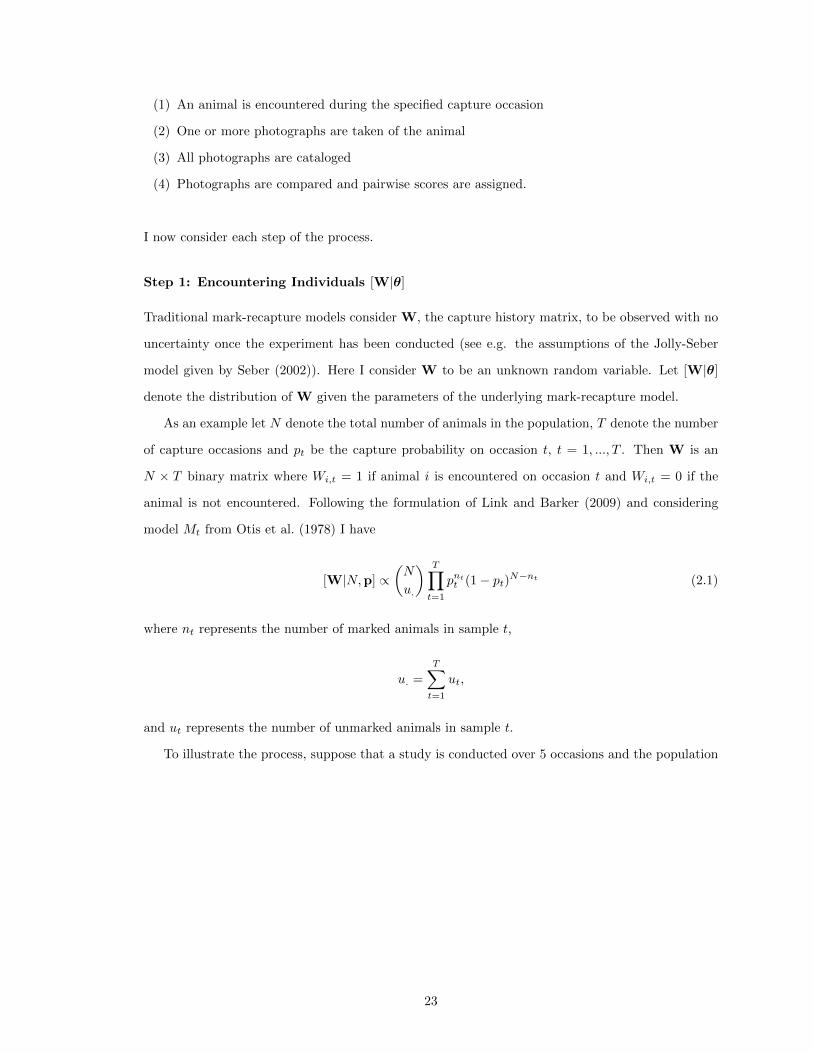
As an example let N denote the total number of animals in the population, T denote the number

of capture occasions and pt be the capture probability on occasion t, t = 1, ..., T . Then W is an

N × T binary matrix where Wi,t = 1 if animal i is encountered on occasion t and Wi,t = 0 if the

animal is not encountered. Following the formulation of Link and Barker (2009) and considering

model Mt from Otis et al. (1978) I have

[W|N,p] ∝(N

u.

) T∏t=1

pntt (1− pt)N−nt (2.1)

where nt represents the number of marked animals in sample t,

u. =

T∑t=1

ut,

and ut represents the number of unmarked animals in sample t.

To illustrate the process, suppose that a study is conducted over 5 occasions and the population

23

consist of a total of 9 individuals. A potential capture occasion matrix is:

W =

1 0 1 0 0

1 0 1 0 1

0 0 0 0 0

1 0 1 0 0

0 1 0 0 0

0 1 0 1 1

0 0 0 0 0

0 1 0 0 0

0 0 1 0 1

indicating, for example, that individual 1 was observed on occasions 1 and 3. Individuals 3 and 7

were not captured during the study since their histories are comprised of only zeros.

Step 2: Photographing Individuals [Y|W, λ]

Our key assumption regarding the photography process is that the distribution of the number of

photographs is the same for all individuals across all occasions. In particular, I model the number

of photographs, given that an individual is encountered, according to a zero-truncated Poisson

distribution with rate parameter λ and expected value

λeλ

eλ − 1.

Let Yi,t denote the number of times individual i was photographed on occasion t. Given Wit = 0

I know that animal i was not photographed on occasion t, thus Yi,t is deterministically 0. Given

Wit = 1 I know that the animal was sighted and therefore photographed. I model the number of

photographs as a zero-truncated Poisson distribution such that,

[Yit|Wit = 1, λ] ∝ λyit

(eλ − 1)yit!. (2.2)

The density of Y is

[Y|W, λ] ∝ (2.3)

N∏i=1

T∏t=1

(λyit

(eλ − 1)yit!

)wit(I[yit = 0])

1−wit .

24

Where I[yit = 0] represents the indicator function such that I[yit = 0] = 1 when yit = 0 and

0 otherwise. Continuing the example from step 1, suppose that the rate parameter of the zero-

truncated Poisson distribution is 3. A potential realization of Y is:

Y =

2 0 1 0 0

1 0 3 0 2

0 0 0 0 0

3 0 2 0 0

0 1 0 0 0

0 4 0 3 3

0 0 0 0 0

0 1 0 0 0

0 0 2 0 1

.

Here individual 1 was photographed twice during the first capture occasion and once during the

third. The 3rd and 7th row of Y contain only zeros because those individuals were never captured

and could not have been photographed.

Step 3: Cataloging the Photographs [X|Y]

Once the photographs are taken they are cataloged and given a unique ID. Consider the example

from above, it can be seen that a total of 29 photographs were taken. For simplicity I assign each

photograph a unique ID ranging from 1 to 29. Information about the occasion on which each photo

was taken and the individual depicted in the photo is summarized by the object X. This information

can be represented in different ways. One such way to visualize X is a structure similar to Y above.

X =

8, 21 · 17 · ·

1 · 4, 13, 16 · 27, 28

· · · · ·

9, 15, 23 · 10, 12 · ·

· 11 · · ·

· 3, 5, 14, 22 · 6, 7, 19 25, 26, 29

· · · · ·

· 18 · · ·

· · 2, 20 · 24

25

In this representation of X each row represents the information from one individual and each col-

umn represents the information from one capture occasion. Notice that the second row contains

information about the second individual. From this it may be inferred that individual 2 was de-

picted in photograph 1 which was taken on the 1st capture occasion and was also photographed in

photographs 4, 13 and 16 on the 3rd capture occasion.

Conditional on Y, which tells us the number of times an individual was photographed per

occasion, and the observed occasion of the photographs I am able to define the sample space for X.

I consider X|Y to be distributed uniformly over the sample space. Let XY be the sample space of

X|Y. Given Y I know the number of photos per individual per occasion. I only need to consider

values of X that agree with Y. All other choices of X occur with probability zero. In what follows

I will show that the cardinality of the space of possible X|Y arrays may be very large even when

the number of photographs is small.

Let Y·t denote the total number of photographs taken on the tth occasion. Then the cardinality

of XY is given by:T∏t=1

[(Y·tY1,t

) N∏i=2

(Y·t −

∑i−1l=1 Yl,t

Yi,t

)].

As an example suppose that:

Y =

2 3 1

1 0 1

1 2 1

so that

Y·1 = 4

Y·2 = 5

Y·3 = 3.

For occasion 1 I have: (4

2

)(2

1

)(1

1

)= 12.

For occasion 2 I have: (5

3

)(0

1

)(2

2

)= 10.

For occasion 3 I have: (3

1

)(2

1

)(1

1

)= 6.

26

Even with only 3 individuals and 12 photographs the cardinality of XY is 720. It is easy to imagine

that XY becomes very large for realistic data sets, and this may cause issues when fitting the model.

In later sections I will implement MCMC to fit the model and care will need to be taken when

choosing initial values because without a reasonable choice of starting value for X the sampler may

take a long time to converge.

Step 4: Generating Scores [Sobs|X,ψ]

Next I consider how the pairwise scores are generated. Let C(X) be the Np ×Np latent matrix of

true match/non-match, where Np represents the total number of photographs. Then Cj1,j2(X) = 1

if the same animal is depicted in both photo j1 and photo j2 and Cj1,j2(X) = 0 otherwise. This

matrix is symmetric by definition and can be computed directly as a function of X.

Consider the previous example. The resulting C(X) matrix has dimension 23× 23, and the first

row of the resulting C(X) is,

(1 0 0 1 0 0 0 0 0 0 0 0 1 0 0 1 0 0 0 0 0 0 0

)

indicating that the same individual was depicted in photographs 1, 4, 13 and 16. Note that the

entries of C(X) are not independent of one another. As an example if entries Cj1,j2(X) = 1 and

Cj2,j3(X) = 1 then the entry Cj1,j3(X) must also equal 1. This property is known as transitivity

(Steorts et al., 2014) and is guaranteed by restricting X to the allowable subspace.

By assumption 2 the scores are generated independently of one another. Further to this I regard

the observed scores conditional on C(X) as draws from a mixture of known densities such that

f(s|Ci,j(X)) = Ci,j(X)fm(s|ψm) + (1− Ci,j(X))fn(s|ψn)

for all i and j where ψm and ψn are the parameters of the density for matches and non-matches

respectively and ψ = (ψm, ψn) is known. Additionally fn and fm are not required to take the same

form. The flexibility of the presented model allows for a different distribution to model the scores

given the latent array X.

27

2.2.2 Inference

In this section I provide a brief outline of how I obtain inference from the proposed model. I fit the

model by applying Bayesian methods that incorporate the CDL

[Sobs,X,Y,W|ψ, λ,θ], (2.4)

where the variables X, Y and W all contain unknown latent variables. Further note that the CDL

can be factored:

[Sobs,X,Y,W|ψ, λ,θ] = (2.5)

[Sobs|X,ψ][X|Y][Y|W, λ][W|θ].

Each of these densities are defined in the previous section and [W|θ] depends on the underlying

mark-recapture model. Figure 2.1 depicts the directed acyclic graph for the general model.

28

θ

W

λ

Y

X

ψ

C

Sobs

Figure 2.1: Directed acyclic graph (DAG) representation of the proposed hierarchical model. Singlearrows denote stochastic relationships and double arrows deterministic relationships. Random nodesare depicted with circles and fixed nodes as rectangles.

As an example the DAG depicting the hierarchical model incorporating model Mt previously

discussed in Chapter 1 can be seen in Figure 2.2.

29

N p

W

λ

Y

X

ψ

C

Sobs

Figure 2.2: Directed acyclic graph (DAG) representation of the proposed hierarchical model. Noticethe only change from the generic DAG are the nodes above W .

Note that further latent variables may be added to the model to simplify construction of the CDL.

For example, in Section 2.3 I employ the Jolly-Seber model and include latent variables representing

times of birth and death for each individual in the population, as described by Schofield and Barker

(2008). The joint posterior distribution is given by:

[θ,W,X,Y, λ|Sobs] (2.6)

∝ [Sobs|X,ψ][X|Y][Y|W, λ][W|θ][λ,θ]

30

where [λ,θ] represents the joint prior.

I implement MCMC to sample from the joint posterior distribution. As part of the process the

missing information in X, Y and W is updated employing information from Sobs and the current

parameter values. The sampler was constructed incorporating both Gibbs steps and Metropolis

within Gibbs steps (Casella and George, 1992; Gilks et al., 1995). Since the dimension of X, W, and

Y depends on θ, RJMCMC motivates the acceptance probability in the Metropolis-Hasting step

(Green, 1995). Details on the MCMC sampler for the Jolly-Seber model applied to the data from

whaleshark.org, described in Section 2.3, are provided in Section 2.3.6.

2.3 Application

2.3.1 Data

The data comprise pairwise scores from 820 photographs taken of whale sharks (Rhincodon typus) in

the northern ecotourism zone of the Nigaloo Marine Park near Exmouth on the North West Cape of

Australia (21◦ 55’59S 114◦ 7’41E) and submitted to whaleshark.org between 2003 and 2008. Whale

sharks are the worlds largest fish and possess unique spot patterns located on the side of the animals

that make photo identification of the animals possible (Holmberg et al., 2008). The photo in Figure

2.3 is representative of the spot patterns. Results from mark-recapture analysis of this data have

been published previously in Holmberg et al. (2009, 2008). The work considers the identity of the

animals in the photographs to be known without error.

31

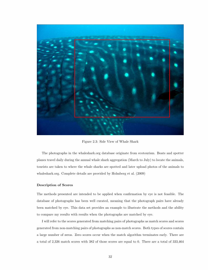
Figure 2.3: Side View of Whale Shark

The photographs in the whaleshark.org database originate from ecotourism. Boats and spotter

planes travel daily during the annual whale shark aggregation (March to July) to locate the animals,

tourists are taken to where the whale sharks are spotted and later upload photos of the animals to

whaleshark.org. Complete details are provided by Holmberg et al. (2009)

Description of Scores

The methods presented are intended to be applied when confirmation by eye is not feasible. The

database of photographs has been well curated, meaning that the photograph pairs have already

been matched by eye. This data set provides an example to illustrate the methods and the ability

to compare my results with results when the photographs are matched by eye.

I will refer to the scores generated from matching pairs of photographs as match scores and scores

generated from non-matching pairs of photographs as non-match scores. Both types of scores contain

a large number of zeros. Zero scores occur when the match algorithm terminates early. There are

a total of 2,326 match scores with 382 of those scores are equal to 0. There are a total of 333,464

32

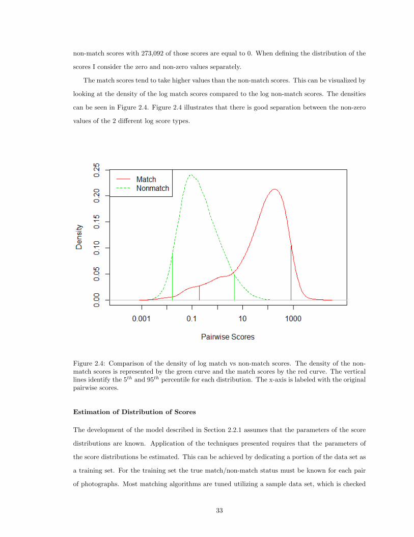
non-match scores with 273,092 of those scores are equal to 0. When defining the distribution of the

scores I consider the zero and non-zero values separately.

The match scores tend to take higher values than the non-match scores. This can be visualized by

looking at the density of the log match scores compared to the log non-match scores. The densities

can be seen in Figure 2.4. Figure 2.4 illustrates that there is good separation between the non-zero

values of the 2 different log score types.

Figure 2.4: Comparison of the density of log match vs non-match scores. The density of the non-match scores is represented by the green curve and the match scores by the red curve. The verticallines identify the 5th and 95th percentile for each distribution. The x-axis is labeled with the originalpairwise scores.

Estimation of Distribution of Scores

The development of the model described in Section 2.2.1 assumes that the parameters of the score

distributions are known. Application of the techniques presented requires that the parameters of

the score distributions be estimated. This can be achieved by dedicating a portion of the data set as

a training set. For the training set the true match/non-match status must be known for each pair

of photographs. Most matching algorithms are tuned utilizing a sample data set, which is checked

33

visually by researchers to see how well the algorithm is working. I make the assumption that the

researchers make no mistakes in their visual inspection of the photographs.

For the whale shark data referenced in Section 2.3.1 the true match/non-match status is known

for the entire data set. I consider the full data set to estimate the distributions for illustration

recognizing that in practice this would not be feasible. Recall from section 2.2.1 that I regard the

observed scores conditional on C(X) as draws from a mixture of known densities such that

f(s|Ci,j(X)) = Ci,j(X)fm(s|ψm) + (1− Ci,j(X))fn(s|ψn)

for all i and j where ψm and ψn are the parameters of the density for matches and non-matches

respectively and ψ = (ψm, ψn) is known. It should be noted that fn and fm are not required to have

the same form. Next I consider the distribution for the match scores, noting that the distribution

for the non-match scores has similar form. One important aspect of the data from the whale shark

study contains a large number of zero scores, for both non-matches and matches, which are associated

with early termination of the scoring algorithm. To accommodate this, I employ a further mixture

distribution providing point mass at 0. The exact formulation is:

fm(si,j |ψm, θm) = I{si,j = 0}θm + (1− I{si,j = 0})(1− θm)g(si,j |ψm).

where g(si,j |ψm) is the density of scores greater than 0 and θm is the probability of observing a zero

score given that the two photographs depict the same individual.

In the case of the modified Groth scores from the whale shark data I found that the non-zero scores

could be adequately modeled as normally distributed after applying the Box-Cox transformation so

that:

g(si,j |ψm) = φ(h(si,j)− µm

σm

)sλm−1i,j

where φ(·) represents the density of the standard normal and ψm = (λm, σm, µm) and

h(Si,j)|Ci,j·∼ N(µm, σ

2m)

with

h(Si,j)|Ci,j =sλmi,j − 1

λm.

34

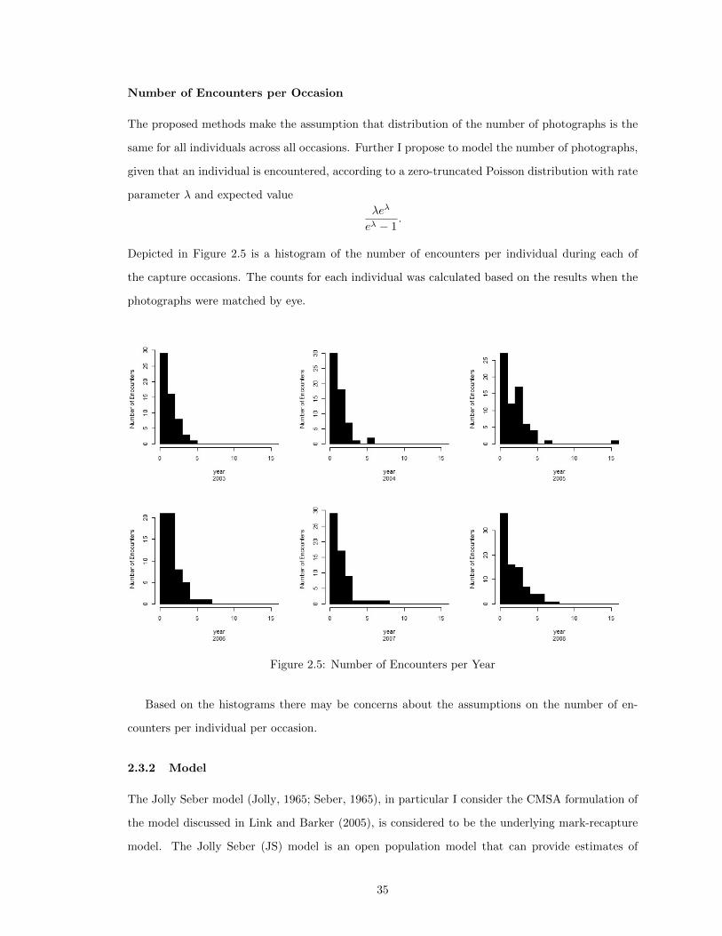
Number of Encounters per Occasion

The proposed methods make the assumption that distribution of the number of photographs is the

same for all individuals across all occasions. Further I propose to model the number of photographs,

given that an individual is encountered, according to a zero-truncated Poisson distribution with rate

parameter λ and expected value

λeλ

eλ − 1.

Depicted in Figure 2.5 is a histogram of the number of encounters per individual during each of

the capture occasions. The counts for each individual was calculated based on the results when the

photographs were matched by eye.

Figure 2.5: Number of Encounters per Year

Based on the histograms there may be concerns about the assumptions on the number of en-

counters per individual per occasion.

2.3.2 Model

The Jolly Seber model (Jolly, 1965; Seber, 1965), in particular I consider the CMSA formulation of

the model discussed in Link and Barker (2005), is considered to be the underlying mark-recapture

model. The Jolly Seber (JS) model is an open population model that can provide estimates of

35

population size, apparent survival and birth rates. The key assumptions of the model are 1) that

probability of capture is the same for each individual within an occasion but can vary across occa-

sions, 2) that the probability for survival is the same for each individual between occasions t and

t+ 1, 3) that the probability for birth is the same for each individual between occasions t and t+ 1,

and 4) these processes are independent between individuals and across time. For more specifics

please see Seber (2002). I provide notation for the model in Table 2.2 and the DAG for the model

can been seen in Figure 2.6.

36

N

ψ

β

b

d

φ

p

W

λ

Y

X

C

Sobs

Figure 2.6: Directed acyclic graph (DAG) representation of the proposed hierarchical model imple-menting the CMSA formulation of the JS model as the underlying Mark-Recapture model.

37

Table 2.2: Additional notation needed for JS modelTerm DefinitionN Total number of individuals available for capture during the studyβt Probability that an individual ever available for capture enters between times t and t+ 1b Latent birth vector of length N , where bi=t denotes the individual was born between

times t− 1 and tφt Probability that an individual alive and in the population at time t, is alive and in the

population at time t+ 1d Latent death vector of length N , where di=t denotes the individual died between times

t and t+ 1pt Probability of capture on occasion t

2.3.3 Inference for the JS Model

I let each pt and φt originate from a standard non-informative prior, Be(1, 1). Further βt has a

Dirichlet(.5) prior, which is also a non-informative prior. The Jeffreys prior was considered for λ,

[λ] ∝ λ− 12 .

This prior is considered non-informative for the Poisson distribution. For N I consider the Jeffreys

prior,

[N ] ∝ 1

N.

2.3.4 Sampler for JS model

I follow the formulation of Link and Barker (2009) when updating p, φ and β. Algorithm 3 outlines

the sampler. Since construction of the model in WinBUGS (Lunn et al., 2000) is not feasible, custom

Initialize β, φ, p, and λInitialize X, W, d, b

1. Update β with a Gibbs step

2. Update φ with a Gibbs step

3. Update p with a Gibbs step

4. Update λ with a Gibbs step

5. Update X, W, d, b with a MH within Gibbs step

Algorithm 3: MCMC algorithm

R code (R Core Team) was written.

38

Figure 2.7: Plot of 3 chains, each chain was generated with a different starting value of X such thatk = .8 + .144h, h = −.25, 0, .25. The data was simulated from a mixture of beta distributions, withthe distribution of the non-zero match scores having mean .8 and variance .144.

2.3.5 Initial Value for X

Without a reasonable starting value for X the chains in the MCMC sampler may take a long time to

converge. I generate the initial value for X with aid of the parameters of the distribution of scores

for the non-zero, matching pairs of photographs, ψm, which are assumed known and the observed

scores. First, I define a threshold, k, such that any score greater than k is assumed to correspond

to a match, i.e. I set the corresponding entries of C(X) = 1. Any observed score greater than k

will be considered a match for the initial value. The constant k can be determined various ways and

should be motivated by the parameters of the score distributions. I recommend setting k equal to

the mean of the non-zero match distribution plus some constant, h, times the variance. In order to

preserve transitivity, closure was taken over the pairs. All other entries of C(X) are set to zero. I

then transform C(X) to X.

In Figure 2.7 I assess the convergence for different values of h. Looking at the plot I can see that

all three chains converge to the true value of N . Similar results were seen for the other parameters

of interest.

39

2.3.6 MCMC Sampling

Here I provide details on the sampler fitting the CMSA formulation of the JS model (Crosbie and

Manly, 1985; Schwarz and Arnason, 1996) as the underlying mark-recapture model. The update of

p, φ and β have been well documented in other texts, such as Link and Barker (2009, Chapter 11),

but are included here for completeness.

Updating the Apparent Birth Probability β

I update β with a Gibbs step. Under a Dirichlet(α) prior,

β|X,θ ∼ Dirichlet(α′)

where α′t = αt +∑Ni=1 I{bi = t}, t = 1, . . . , T .

Updating the Apparent Survival Probability φ

I update each φt with a Gibbs step. Under a Beta(αφ, βφ) prior, for φt,

φt|X,θ ∼ Beta(M+t −Dt − αφ, Dt + βφ)

where M+t represents the number of animals alive immediately following occasion t and

Dt =

N∑i=1

T{di = t}

represents the number of animals that die between samples t and t+ 1.

Updating the Capture Probability p

I update each pt with a Gibbs step. Under a Beta(αp, βp) prior for pt

pt|X,θ ∼ Beta(mt + αp,Mt −mt + βp)

where mt denotes the number of animals that are captured on occasion t.

40

Updating the Rate of Photography λ

I consider λ to the be the rate parameter of a zero truncation Poisson distribution. Conditional on

λ

[Y |W, λ] ∝ (2.7)

N∏i=1

T∏t=1

(λyit

(eλ − 1)yit!

)wit(I[yit = 0])

1−wit .

The Jeffreys prior for the Poisson distribution was considered for λ,

[λ] ∝ λ− 12

which leads to the following full conditional distribution

∝N∏i=1

T∏t=1

(λyit−.5

(eλ − 1)yit!

)wit(I[yit = 0])

1−wit .

I sample from this distribution by implementing a Metropolis-Hastings step with the candidate λ

drawn from an Exponential(1, 1) distribution.

Updating the Complete Data

To simplify the description of the update for the complete data I introduce a different formulation

of X than the one presented in Section 2.2.1. I can visualize X as a data frame with 2 columns

in which the ith row of the data frame contains information about the ith photograph. The first

column denotes the occasion the photo was taken and the second column denotes the individual

that is depicted in the photograph. Recall the example from Section 2.2.1 where,

X =

8, 21 · 17 · ·

1 · 4, 13, 16 · 27, 28

· · · · ·

9, 15, 23 · 10, 12 · ·

· 11 · · ·

· 3, 5, 14, 22 · 6, 7, 19 25, 26, 29

· · · · ·

· 18 · · ·

· · 2, 20 · 24

41

With the new formulation X will have 29 rows. The first 6 rows are provided below

1 2

3 9

2 6

3 2

2 6

4 6

and show, for example, that the first photograph was taken on the 1st capture occasion and depicts

individual 2. This formulation of X contains the same information as the previous formulation but

is easier to work with when updating the complete data.

Adding or Deleting an Individual I

The update of adding or deleting an individual is the most complicated type of update because the

addition of a new individual requires sampling new times of birth and death and a new capture

history, and to move photographs between the individuals (if the newly generated individual is

captured at least once). Let W′,Y′,X′, b′ and d′ denote the candidate W,X,Y, b and d respectively.

To create the candidates I randomly decide to add a new individual with probability q or delete an

individual with probability 1− q. By default I set q = .5. Below I outline the process of generating

the candidates once the choice to add or delete an individual is made.

• Adding a new individual

Data for a new individual in the population is simulated in the following steps:

1. Generate an ID for the new individual:

Simulate j ∼ Uniform(1, . . . , N + 1).

2. Generate information for the new individual:

i) Simulate b′j |β.

ii) Simulate d′j |b′i,φ.

iii) For t = 1, . . . , T ;

If t < b′j or t > d′j set w′j,t = 0 and Y ′j,t = 0.

Else,

a) Simulate w′j,t ∼ Bernoulli(pt).

42

b) If wj,t = 0 set Y ′j,t = 0. Otherwise generate Y ′j,t ∼ ZTPoisson(λ).

c) If Y ′j,t > 0 let v be a vector of length Y ′j,t. Uniformly sample v from all possible

samples of size Y ′j,t from the IDs of photos taken on occasion t.

3. Create X′, b′, and d′:

i) Set X′ = X.

ii) For k = 1, . . . , Np

If X[k, 2] < j, set X′[k, 2] = X[k, 2]

Else set X′[k, 2] = X[k, 2] + 1

iii) Set X′[v, 2] = j.

iv) Set b′ = (b1, . . . , bj−1, b′j , bj , . . . , bN ).

v) Set d′ = (d1, . . . , dj−1, d′j , dj , . . . , dN ).

• Deleting an individual

1. Select an individual ID to delete:

Simulate j ∼ Uniform(1, . . . , N).

2. Create X′, b′, and d′:

i) Set X′ = X

ii) For k = 1, . . . , Np

If X[k, 2] < j, set X′[k, 2] = X[k, 2]

Else set X′[k, 2] = X[k, 2]− 1

iii) Set b′ = (b1, . . . , bj−1, bj+1, . . . , bN ).

iv) Set d′ = (d1, . . . , dj−1, dj+1, . . . , dN ).

v) For each k such that X[k, 2] = j, generate X[k, 2] ∼ Uniform(1, . . . , N).

2.3.7 Updates for Mixing

Although Markov chains previously defined will converge to the proper distribution, I recommend

three additional updates to aid in mixing.

Adding or Deleting an individual II

The second update of adding or deleting an individual improves the mixing of the population size

by adding or deleting multiple individuals not seen in the study (i.e., with all zeros in their capture

history). As result X is only modified by relabeling of the individuals and not by moving photographs

43

from one individual to another. To create the candidate I randomly decide to add a new individual

with probability q or delete an individual with probability 1 − q. By default I set q = .5. Below

I outline the process of generating the candidates once the choice to add or delete an individual is

made.

• Adding a new individual

Data for a new individual in the population is simulated in the following steps:

1. Generate an ID for the new individual:

Simulate j ∼ Uniform(1, . . . , N + 1).

2. Generate information for the new individual:

i) Simulate b′j |β.

ii) Simulate d′j |b′i,φ.

iii) For t = 1, . . . , T set w′j,t = 0 and Y ′j,t = 0.

3. Create X′, b′ and d′:

i) Set X′ = X

ii) For k = 1, . . . , Np

If X[k, 2] < j, set X′[k, 2] = X[k, 2]

Else set X′[k, 2] = X[k, 2] + 1

iii) Set b′ = (b1, . . . , bj−1, b′j , bj , . . . , bN ).

iv) Set d′ = (d1, . . . , dj−1, d′j , dj , . . . , dN ).

• Deleting an individual

1. Select an individual ID to delete:

i) Let K be the set of k such that W[k, t] = 0 for all t. Simulate j ∼ Uniform(K).

2. Create X′, b′, and d′:

i) Set X′ = X

ii) For k = 1, . . . , Np

If X[k, 2] < j, set X′[k, 2] = X[k, 2]

Else set X′[k, 2] = X[k, 2]− 1

iii) Set b′ = (b1, . . . , bj−1, bj+1, . . . , bN ).

iv) Set d′ = (d1, . . . , dj−1, dj+1, . . . , dN ).

44

Updating the Latent Birth Vector b

I update bi with a Gibbs step. The full conditional distribution of bi is a categorical distribution

with sample space {1, . . . , ci} where

ci =

di if ωi = 0

min{t : ωit = 1} otherwise

and probability vector θi = (θi1, . . . , θici)′ such that

θij ∝ βjci−1∏k=j

(φk(1− pk))

and the empty product is set equal to 1 if j = ci.

Updating the Latent Death Vector d

I update di with a Gibbs step. The full conditional distribution of di is a categorical distribution

with sample space {li, . . . , T} where

li =

bi if ωi = 0

max{t : ωit = 1} otherwise

and probability vector ζi = (ζili , . . . , ζiT )′ such that

ζij ∝j−1∏k=li

(φk(1− pk)) (1− φj)

and the empty product is set equal to 1 if j = li. Note that for the update of d and b there

appears to be an error in Link and Barker (2009). The probabilities for d need to include p and the

probabilities for b need to include p and φ.

2.3.8 Need for Reversible Jump MCMC

As discussed in Chapter 1, RJMCMC is required when the dimension of a random variable changes

across the sample space. Recall that RJMCMC is often implemented when it is desirable to sample

from potential candidate models, for example if choosing different regression models. For this reason

RJMCMC algorithms are often summarized in terms of sampling from potential models Mk, where

45

k = 1, . . . ,K and θk is the parameter set for model model k with dimension dk (Gelman et al., 2014).

In the case of my work I am not sampling from potential models, but rather potential dimensions. In

particular the dimension of both the latent death vector d and the latent birth vector b vary across

the the respective sample spaces. This occurs because the length of each vector is dependent on the

population size N which varies. As a reminder the RJMCMC algorithm is described in Algorithm

4.

1. Starting with model Mk with parameter vector θk, (k, θk), propose a new model Mk∗ withprobability Jk,k∗ and generate an augmenting random variable u from proposal densitym(u|k, k∗, θk).

2. Determine the proposed model’s parameters, (θk∗ , u∗) = gk,k∗(θk, u)

3. Define the ratio

r =p(y|θk∗ ,Mk∗)p(θk∗ |Mk∗)πk∗

p(y|θk,Mk)p(θk|Mk)πk

Jk∗,km(u∗|k∗, k, θk∗)Jk,k∗m(u|k, k∗, θk)

∣∣∣∣∇gk,k∗(θk, u)

∇(θk, u)

∣∣∣∣and accept the new model with probability min(r,1).

Algorithm 4: RJMCMC Algorithm

Below I show that in the update of b and d for the previously described sampler the absolute

determinate of the Jacobian equals 1. Since the value is 1 I am left with the usual Metropolis

Hastings acceptance probability. The jumping proposal m(N ′|N) is defined as follows:

N ′ =

N + 1 with probability q

N − 1 with probability 1− q.

Consider b and suppose that N ′ = N + 1. Further suppose that I add an individual with subscript

m according to the proposal distribution outlined in Section 2.3.6. Then,

gN,N ′(b, u) = [b′1, b′2, . . . , b

′N+1].

where,

b′ = (b1, . . . , bm−1, u, bm, . . . , bN )

and

u = b′m

u′ = b′m

46

Therefore the Jacobian takes the form,

∣∣∣∣∣∣∣∣∣∣∣∣∣∣∣∣∣∣∣∣∣∣∣

∂b′1∂b1

. . .∂b′m−1

∂b1

∂b′m∂b1

∂b′m+1

∂b1. . .

∂b′N′

∂b1... . . .

......

... . . ....

∂b′1∂bm−1

. . .∂b′m−1

∂bm−1

∂b′m∂bm−1

∂b′m+1

∂bm−1. . .

∂b′N′

∂bm−1

∂b′1∂u′ . . .

∂b′m−1

∂u′∂b′m∂u′

∂b′m+1

∂u′ . . .∂b′N′

∂u′

∂b′1∂bm

. . .∂b′m−1

∂bm

∂b′m∂bm

∂b′m+1

∂bm. . .

∂b′N′

∂bm... . . .

......

... . . ....

∂b′1∂bN

. . .∂b′m−1

∂bN

∂b′m∂bN

∂b′m+1

∂bN. . .

∂b′N′

∂bN

∣∣∣∣∣∣∣∣∣∣∣∣∣∣∣∣∣∣∣∣∣∣∣

=

∣∣∣∣∣∣∣∣∣∣∣∣∣∣∣∣∣∣∣∣∣∣∣

1 . . . 0 0 0 . . . 0

... . . ....

...... . . .

...

0 . . . 1 0 0 . . . 0

0 . . . 0 1 0 . . . 0

0 . . . 0 0 1 . . . 0

... . . ....

...... . . .

...

0 . . . 0 0 0 . . . 1

∣∣∣∣∣∣∣∣∣∣∣∣∣∣∣∣∣∣∣∣∣∣∣Therefore the absolute determinant of the Jacobian is equal to 1. For the reverse move I can take

the inverse and find a similar result. Additionally the calculation for the latent death vector, d, is

similar.

2.4 Results

In this section I provide the results from the application of the Score Based Mark-Recapture model

to simulated data and data from whaleshark.org.

2.4.1 Simulated Data

Prior to the development of the Score Based Mark-Recapture model, fitting the JS model required

that the capture histories be treated as fixed and constructed from the relationship between pho-

tographs while ignoring the inherent uncertainty in the matching process. A simulation study was

conducted to illustrate the potential bias in parameter estimates when researchers recreate the cap-

ture histories and ignore the inherent uncertainty in the matching process which may lead to falsely

labeling two photographs as a matching pair or missing a true matching pair. The primary objec-

tive was to asses the bias in the estimates as the occurrence of false matches and false non-matches

increased. I simulated data under the CMSA formulation of the JS model with T = 5, N = 200,

β = (.6, .1, .1, .1, .1), φt = .8 and pt = .5 for t = 1, . . . , 5, and λ = 3. These values were chosen be-

cause they represent a species that has high survival probability and moderate capture probability

similar to the whale sharks. Additionally I simulated scores under 3 different beta mixtures, with

each mixture having a different amount of overlap between the match and non-match portion of the

mixture.

For each Beta mixture 100 data sets were simulated. To recreate the effect of the falsely labeling

47

some pairs of photographs as matches or non-matches I considered the underlying distribution of the

scores. All scores higher than than the .05 quantile of the match score distribution were labeled as

matches, whereas all scores lower than the .95 quantile of the non-match distribution were labeled as

non-matches. As the overlap between the distributions increased the occurrence of false non-matches

and matches increased. Transitive closure was taken over the matrix of match/non-match status

of the photographs and the capture occasion matrix was recreated to reflect the false matches and

non-matches. The model was fit utilizing MCMC with 50,000 burn in and 50,000 iterations. Located

in Table 2.3 are the results from the simulation of credible intervals for abundance. I found that

when there was a small overlap between the distributions few errors were made and there was little

to no bias. When the overlap increased the number of errors grew and the credible intervals failed

to adequately cover the true value of abundance and tended to underestimate the population size.

This result was not surprising. In the presence of false matches transitive closure over the matrix of

true match status has the potential to assign all photographs to a single individual and the estimate

of population size is underestimated since fewer individuals are observed. This is discussed further

in Chapter 3.

To assess the performance of the Score Based Mark-Recapture model I conducted a second

simulation study. The primary objectives were to determine how the performance was affected by

the number of photographs, per individual and per occasion, and by the overlap in the distributions

for the match and non-match scores. I simulated data under the CMSA formulation of the JS model

with T = 5, N = 200, β = (.6, .1, .1, .1, .1), φt = .8 and pt = .5. Again these values were chosen

because they represent a species that has high survival probability and moderate capture probability

similar to the whale sharks. In order to see how well the model performed when the average number

of photographs per individual per occasion increased I simulated data both when λ = 1 and λ = 3.

Additionally I simulated scores under 3 different beta mixtures, with each mixture having a different

amount of overlap between the match and non-match portions of the mixture.

For each set of parameters 100 data sets were simulated, the model was fit utilizing MCMC with

50,000 burn in and 50,000 iterations. I also simulated 100 data sets where for each data set I utilized

the true value of W to fit CMSA model. By considering the true value of W as data to fit the

model I was able to examine the behavior of credible intervals when the uncertainty of the photo

identification is not an issue. For these intervals the average credible interval width was 62.8 with a

standard deviation of 23.45. I compared the average credible width of the intervals from the CMSA

model to the credible interval widths from the proposed Score Based Mark-Recapture model and

found that the Score Based Mark-Recapture model produced credible intervals with similar mean

48

Table 2.3: The first column lists the simulation number. The second and third columns denotethe values for the parameters of the beta mixture: (αm, βn) and (αn, βm) respectively. For eachsimulation the value of α for the Beta distribution of non-match scores and the value βm for thematch scores was equal to 2. The fourth column denotes the percentage of overlap between thematch and non-match distributions. The fifth column list the percent coverage of the parameter Nfor 100 credible intervals.

Simulation (αm, βn) (αn, βm) % Overlap % Coverage1 12 2 0.3 922 10 2 1.2 83 8 2 3.9 0

width. Located in Table 2.4 are the results from the simulation of credible intervals for abundance.

I found that when λ = 3 the coverage was high even when there was a large overlap between the

distributions. Further when λ = 1 and the overlap between the distributions was small the coverage

was also high. When λ = 1 and there is a large overlap between the distributions I found that the

credible intervals tend to underestimate the population size.

Table 2.4: The first column lists the simulation number. The second column identifies the valueof λ. The third and fourth columns denote the values for the parameters of the beta mixture:(αm, βn) and (αn, βm) respectively. For each simulation the value of α for the Beta distribution ofnon-match scores and the value βm for the match scores was equal to 2. The fifth column denotesthe percentage of overlap between the match and non-match distributions. The sixth column listthe percent coverage of the parameter N for 100 credible intervals. The last column list the meancredible interval width.

Simulation λ (αm, βn) (αn, βm) % Overlap % Coverage Mean CI Width1 3 8 2 3.9 96 69.12 3 6 2 12.5 96 63.93 3 4 2 37.5 94 60.294 1 8 2 3.9 91 62.585 1 6 2 12.5 85 61.396 1 4 2 37.5 20 48.2

2.4.2 Whale Shark Data Set

I began by fitting the Score Based Mark-Recapture model then since the true match/non-match

status for the whale shark data is known, I fit the CMSA model using the true match/non-match

status of the pairs of photographs as data. Each sampler was ran with a single chain of 600,000

iterations, which included a burn in of 300,000 iterations. I was able to create the true value of X

since the true match and non-match relationships were known for the data, and considered it as a

starting value for X when fitting the Score Based Mark-Recapture model as well as the CMSA model.

49

Table 2.5: The first column lists the simulation number. The second column identifies the valueof λ. The third and fourth columns denote the values for the parameters of the beta mixture:(αm, βn) and (αn, βm) respectively. For each simulation the value of αn for the Beta distribution ofnon-match scores and the value βm for the match scores was equal to 2. The fifth column gives thepercentage of overlap between the match and non-match distributions. The last five columns givethe coverage of the parameter φ for 100 credible intervals.

Simulation λ (αm, βn) (αn, βm) % Overlap % p1 % p2 % p3 % p4 % p51 3 8 2 3.9 95 97 100 100 1002 3 6 2 12.5 100 100 100 100 973 3 4 2 37.5 99 100 100 99 954 1 8 2 3.9 96 99 100 100 995 1 6 2 12.5 97 100 99 100 1006 1 4 2 37.5 92 97 99 100 94

Table 2.6: The first column list the simulation number. The second column identifies the valueof λ. The third and fourth columns denote the values for the parameters of the beta mixture:(αm, βn) and (αn, βm) respectively. For each simulation the value of αn for the Beta distribution ofnon-match scores and the value βm for the match scores was equal to 2. The fifth column gives thepercentage of overlap between the match and non-match distributions. The last four columns givethe coverage of the parameter p for 100 credible intervals.

Simulation λ (αm, βn) (αn, βm) % Overlap % φ1 % φ2 % φ3 % φ41 3 8 2 3.9 93 97 100 1002 3 6 2 12.5 92 97 93 1003 3 4 2 37.5 96 96 90 994 1 8 2 3.9 88 95 96 1005 1 6 2 12.5 93 93 93 1006 1 4 2 37.5 69 84 87 100

In practice I recommend running multiple chains to check for convergence as well as implementing

standard checks for convergence such as the Brooks Gelman Ruben diagnostic, but did not in this

case since I are comparing the Score Based Mark-Recapture model results to the CMSA model

results (Gelman and Rubin, 1992; Brooks and Gelman, 1998).

Provided in Figures 2.8 and 2.9 are box plots of values sampled from the posterior distribution of

φt and pt respectively from the CMSA model and the Score Based Mark-Recapture model. The fig-

ures illustrate that the posterior distributions for the apparent survival and the capture probability

across time are similar for the two models. Further I found that the posterior distribution of birth

probability utilizing the Score Based Mark-Recapture model was very similar to the CMSA model

suggesting that in the absence of knowing the true match/non-match status of the photographs the

Score Based Mark-Recapture model is able to give credible intervals similar to those of current meth-

ods that require the capture histories be known. Additionally the credible intervals for abundance

50

was slightly wider for the Score Based Mark-Recapture model compared to the CMSA model. The

wider interval can be explained by the additional uncertainty of matching the photographs to one

another.

Figure 2.8: Box plots comparing the posterior distributions of the survival probabilities, φt, for theCMSA model (blue) and the Score Based Mark-Recapture model (green). The box represents theextents of the first and third quartiles of the posterior and the vertical line the median. The tailsextend to the smallest and largest values sampled from the posterior.

51

Figure 2.9: Box plots comparing the posterior distributions of the survival probabilities, pt, for theCMSA model (blue) and the Score Based Mark-Recapture model (green). The box represents theextents of the first and third quartiles of the posterior and the vertical line the median. The tailsextend to the smallest and largest values sampled from the posterior.

2.5 Discussion

I have presented the Score Based Mark-Recapture model that addresses the issue of misidentification

in photographic identification. By considering the pairwise scores as data to fit the model I am able

to reduce the need for researchers to visually compare the photographs. Additionally I am able

to utilize information from pairs of photographs that would have previously been discarded due

to an unidentifiable match/non-match status. The whale shark example illustrates that the Score

Based Mark-Recapture model provides similar posterior estimates considering the pairwise scores

as data compared to the CMSA model that requires the true match/non-match status of the pairs

of photographs be known. This provides reassurance that one can rely on the results of the Score

Based Mark-Recapture model without having researchers visually confirm match/non-match status.

52

One area of concern seen in the previous section is when λ = 1 and there is a large overlap between

the distributions and the credible intervals tend to underestimate abundance. The underestimation

is likely due to not enough data to over power the prior and the estimate being drawn towards the

prior mean. In cases when the match and non-match scores have a large amount of overlap and

λ > 1 more data is needed for reliable credible intervals.

Although I consider the CMSA formulation of the JS model as the underlying mark-recapture

model the Score Based Mark-Recapture model can easily be altered to incorporate a different mark-

recapture model. Altering the model to incorporate a different underlying model will require that

the MCMC sampler algorithm be changed. The necessary changes may be elementary or complex

depending on the chosen model.

As previously discussed the Score Based Marked-Recapture model makes four primary assump-

tions. Provided again for convenience they are:

(1) Occasions on which each photograph is taken is known without error.

(2) Scores are independent of one another.

(3) The distribution of the number of photographs per individual is the same on all capture

occasions.

(4) All assumptions for the underlying mark-recapture model hold.

Assumption 1 is critical, the model is able to address the uncertainty of the identification of the

animal depicted in a photograph but cannot address uncertainty about location or time a photograph

was taken. Violation of assumption 2 is possible but would require a joint distribution of scores to be

defined. Assumptions 3 is made for simplicity and can be modified. Modification of the assumption

3 would require a large number of photographs if the distribution of photographs is allowed to vary

by individual and occasion. Assumption 4 depends on the underlying mark-recapture model and in

part can be relaxed if the framework of the underlying mark-recapture model allows.

Although not examined in this work; covariates collected during the study could provide informa-

tion on both identity and parameter estimation. In future work I plan to modify the MCMC sampler

to incorporate information from covariates such as gender and space to help influence the determi-

nation of match and non-match status. Further, covariates could also be included in the underlying

mark-recapture model. This addition of covariates is feasible but would require modifications to the

data structure and MCMC sampler.

One downside to the Score Based Mark-Recapture model is fitting the model with MCMC may be

computationally intensive. As the number of available photographs grows so does the computation

53

time. In future work I would like to explore ways to simplify the process of fitting the model

by approximating the posterior distributions instead of sampling directly. I believe it is possible to

implement the information from pairwise scores as data to make valid inference about the parameters

of interest using a reasonable approximation. As previously discussed Fewster et al. (2016) presents a

method that considers capture-recapture estimation without capture histories utilizing the pairwise

comparison between records. Presented in the paper is the implementation of a pseudo-likelihood

estimation process to aid in estimation. The methods presented in the paper focus on inference

about abundance and distinct animal encounters. Further the method requires that an contrast

process where the intensity of the contrast function peaks at short distances. This is not reasonable

for the pairwise scores from photographs. Scores for matches tend to be high suggesting the need for

the intensity of the contrast function to peak at large distances. This problem could be potentially

alleviated by taking the inverse of the pairwise scores. Further I found that a pairwise score of 0 does

not necessarily suggest that a pair is a non-match, rather a score of zero suggest that the algorithm

attempted to create a score but was unable to. How to handle the zero scores using the method is

not immediately evident.

54

Chapter 3

Incorporation of Auxiliary Data and Record Linkage Methods to Improve

Computational Efficiency

3.1 Introduction

Previous chapters discussed photographic identification and the role photographs of unique markings

of animals play in providing researchers with a noninvasive method for marking and identifying

animals. In Chapter 2 the Score Based Marked-Recapture model was introduced and is able to

model the inherent uncertainty in photographic identification. In this chapter improvements for the

computational efficiency of the methods presented in Chapter 2 by a priori reducing the sample

space of C(X) will be presented. In order to extend the methods I borrow concepts from the field of

record linkage to provide an approximation of the posterior distribution reducing the sample space

of C(X) in a reasonable manor. The implementation of record linkage in photographic identification

is a fairly new idea. Prior to discussing the proposed methods I will provide some background to

the field of record linkage and discuss how record linkage techniques have already been applied to

photographic identification.

3.1.1 Photographic Identification in a Record Linkage Framework

The field of record linkage deals with matching individuals given catalogs of records that need to

be cross referenced. For example one may have a list of customers for two utility companies and

would like to identify which customers receive service from both companies. Customers provide

information to each company such as name, address and phone number. This information creates

a record for each individual which are then cross referenced between companies to determine which

customers are receiving service from both companies. At first glance this seems like an easy task

but people change names, move and get new phone numbers resulting in the same person providing

two different records. Record linkage techniques address the uncertainty in the records.

The issue of deciding which unique animals are depicted in a catalog of photographs may be

viewed in a record linkage framework by considering the photographs of the animals as records and

it is necessary to make a decision as to which of the photographs depict the same animal. If two

distinct catalogs of photographs are available then the situation is similar to the utilities company

example. This occurs when individuals can only be photographed once on each occasion in which

case one could consider the photographs in a single occasion as a catalog then simply match across

55

occasions. Usually photographs are collected over time and placed into a single catalog and the goal

is to identify the unique animals represented by the photographs in the catalog. Record linkage can

be applied in both scenarios.

The seminal work of Fellegi and Sunter (1969) laid the foundation for record linkage and provided

a fundamental theorem that defined optimal record linkage rules. The paper considers matching

records, which consist of categorical information similar to the utilities example above, across two

catalogs. With the goal of the paper being to decide if two records, one from each of the catalogs,

correspond to the same individual or not. The work describes three decisions that may be made in

regards to each possible pair of records from the two catalogs. The three decisions can be referenced

as a link meaning that the same individual is represented in the two records, potential link meaning

that the same individual may be represented in the two records, and non-link meaning that two

different individuals are represented by the records. There are two types of errors that may be

committed. If it is decided that a pair of records is a link when in fact it is not or it is decided

that the pair of records is not a link when in fact it is. Ideally the probability of these errors will

be small. Additionally I would like to minimize the number of pairs assigned to potential link since

the match status of this group is unknown. According to Fellegi and Sunter (1969) a linkage rule

assigns probabilities of appointing a pair of records to either being a link, potential link or non-link.

Further they define an optimal linkage rule, to be one which minimizes the number pairs assigned

to the potential link at some pre-specified error levels. In Section 3.2 I will define a similar rule to

aid in a priori deciding which photographs are matches and non-matches.

In order to address photographic misidentification in a record linkage framework I consider a

single set of photos and wish to identify which photos depict the same individual within the set.

The process of applying record linkage to a single data set is known as de-duplication (Steorts et al.,

2014). One of the issues with de-duplication is that any rule which assigns photo A and photo

B as a match, and also matches photo B and photo C, must also identify photos A and C as a

match. Monge (2000) solves the duplication problem by presenting an ad hoc method which applies

transitive closure by forcing closure. The paper states “If record R1 is a duplicate of record R2,

and record R2 is a duplicate of record R3, then by transitivity R1 is a duplicate of record R3.”

Monge (2000, p 4) Since the method applies transitive closure by creating matches it relies on the

assumption that there are few true duplicates in the files. The paper further explains why this

assumption is necessary, “Transitivity is true by definition if duplicate records concern the same

real-world identity, but in practice there will always be errors in computing pairwise ‘is a duplicate

of’ relationships, and transitivity will propagate these errors. However, in typical databases, sets

56

of duplicate records tend to be distributed sparsely over the space of possible records, and the

propagation of errors is rare.” In the case of photographic identification there is no guarantee that

that the duplicate records will be distributed sparsely over the space of possible records. In fact if

the rate of photography is high and probability of capture is also high there will be a large number

of duplicate records. In Chapter 2 transitive closure was applied when specifying a starting value

for X. In this chapter I will further implement transitive closure in conjunction with a rule similar

to that of Fellegi and Sunter (1969) to a priori reduce the sample space of C(X).

The 2011 paper A Hierarchical Bayesian Approach To Record Linkage And Population Size

Problems, Tancredi et al. (2011) examines estimating population sizes implementing a hierarchical

Bayesian approach, which can be adapted for both capture-recapture studies and record linkage

problems. For photographic identification they consider the physical characteristics of the pho-

tographs as data, this differs from my approach in that I consider the pairwise scores between the

photographs as data. As discussed in Chapter 2 the Scored Based Mark-Recapture model is able to

estimate a wide variety of parameters by incorporating an underlying mark-recapture model where

as Tancredi et al. (2011) only focuses on the estimation of abundance.

More recent work in record linkage has developed methods which borrow from the field of graph

theory. The challenge of matching photographs to the unique individuals depicted in the photographs

can be visualized with a bipartite graph. A bipartite graph is a graph with 2 disjoint sets of nodes

such that each node in one set maps to one node in the other. The graphing problem is to create the

edges (Bondy and Murty, 2008). It’s worth noting that the mapping is not one-to-one. I.e., multiple

nodes in the first set may map to the same node in the second set. It is possible to think of photo

identification as a problem of having two sets of nodes: one set for the individuals depicted in the

photograph and one set for the actual photographs. The matching process considers assigning edges

which connect each photograph node to an individual node in such a way that no two edges share

a node representing a photograph. In short is it possible to connect photographs to individuals so

that each photograph is connected to only one individual. Sadinle and Fienberg (2013) look at the

application of graph theory to solve the bipartite matching problem. Steorts et al. (2014) builds

on the the work of Sadinle and Fienberg (2013) and takes a Bayesian approach considering more

than two list with duplicates within each list. Matches are represented by a bipartite graph in which

records are linked directly to the true latent individual and indirectly to the other records. The paper

promotes the application of a hybrid MCMC algorithm to sample from the posterior distribution

(Steorts et al., 2014). My work does not incorporate graph theory. The reason being that methods

which implement graph theory require data from the nodes, i.e. data which originates from single

57

photographs, whereas my methods consider data from the edges, i.e. data which originates from the

pairwise comparison of photographs.

My intention is to implement record linkage techniques to improve the efficiency of the methods

presented in Chapter 2. The Score Based Mark-Recapture model presented in Chapter 2 includes

the latent variable C(X). When fitting the model I employed MCMC, which required sampling

from the space C(X) conditional on Y , which may be extremely large. One way to improve speed

of computation is to limit the sample space of C(X) in such a way that I am able to achieve a

reasonable approximation to the posterior distribution of the parameters of interest. I propose to

limit the sample space by incorporating record linkage techniques to a priori choose match and non-

match pairs which will remain fixed during sampling. The addition of the record linkage techniques

will also require a new custom sampler.

3.2 Methods

3.2.1 Restricting the Sample Space of C(X)

Recall from Chapter 2 that I considered a data set comprised of all possible pairwise scores from a

set of photographs. I would like to infer from the scores the true match/non-match status of each

pair, represented by C(X) which is a Np×Np binary matrix, where Np represents the total number

of photographs. Then Cj1,j2(X) = 1 if the same animal is genuinely depicted in both photo j1 and

photo j2 and Cj1,j2(X) = 0 otherwise. This matrix is symmetric by definition and can be computed

directly as a function of X. Where X contains information specifying the occasion on which each

photograph was taken and which individual is depicted in each photograph. Previously I considered

each element of C(X) to be stochastic and sampled from the space of all possible realizations of

C(X) conditional on Y, where Y is a N × t matrix and Yi,t denotes the number of times individual

i was photographed on occasion t, t = 1, . . . , T . Further I illustrated that C(X) conditional on Y

potentially has a large sample space and sampling from the space may be computationally intensive.

I propose to a priori select some elements of C(X) to be deterministically one or zero which has the

potential to drastically reduce the cardinality of the sample space and alleviate the computational

complexity.

Let CY be the sample space of C(X)|Y. Given Y the number of photos per individual per

occasion is known and it is only necessary to consider values of C(X) which agree with Y. All other

choices of C(X) occur with probability zero. Further suppose that a priori the true value of some

elements of C(X) is known. These known values are now deterministic and I will refer to these

58

values as fixed. Fixing elements of C(X) will place restrictions on CY , since some of the elements

of CY will now occur with probability zero and will greatly reduce the cardinality of the sample

space. There are two choices that may be made when a priori fixing elements of C(X): a pair of

photographs is a match meaning that Cj1,j2(X) = 1 deterministically or a pair of photographs is a

non-match meaning that Cj1,j2(X) = 0 deterministically. Depending on the available information it

may be possible to a priori fix matches, non-matches or both.

In order to illustrate the effect of fixing elements of C(X) on the cardinality of CY I will revisit

an example from Chapter 2. Suppose that I have the following realization of Y:

Y =

2 0 1 0 0

1 0 3 0 2

0 0 0 0 0

3 0 2 0 0

0 1 0 0 0

0 4 0 3 3

0 0 0 0 0

0 1 0 0 0

0 0 2 0 1

.

Previously I let Y·t denote the total number of photographs taken on the tth occasion and stated

that the cardinality of CY is given by:

#CY =

T∏t=1

[(Y·tY1,t

) N∏i=2

(Y·t −

∑i−1l=1 Yl,t

Yi,t

)].

In this example there are only 29 photographs and the cardinality of CY is 181,440,000. It is easy

to image that as the number of photos increases so will the cardinality of CY resulting in a large

sample space which will be computationally expensive to explore.

In order to illustrate the reduction in the cardinality of CY which occurs when fixing elements of

C(X) I will consider three cases:

1. Predetermining non-matches

2. Predetermine matches

3. Predetermine both matches and non-matches.

59

For now I assume that no errors are made when fixing elements of C(X). In order to illustrate

the restrictions I will work with X and the sample space XY . Recall that there is a one-to-one

relationship between C(X) and X, therefore the cardinality of CY and XY are the same.

Case 1: Predetermined Non-Matches

Predetermining non-matches in X introduces what I will denote as non-match restrictions on XY . A

non-match restriction occurs when it is a priori determined that Cj1,j2(X) = 0 deterministically, for

some photographs j1 and j2. One can think of X as an array with some rows containing photo ID’s

with non-match restrictions and some rows containing rows with no non-match restrictions. The

goal is to to generate candidate X’s which agree with the non-match restrictions on XY . Consider

the previous realization of X from Chapter 2,

X =

8, 21 · 17 · ·

1 · 4, 13, 16 · 27, 28

· · · · ·

9, 15, 23 · 10, 12 · ·

· 11 · · ·

· 3, 5, 14, 22 · 6, 7, 19 25, 26, 29

· · · · ·

· 18 · · ·

· · 2, 20 · 24

Suppose that a priori I am able to determine the following:

• Photos 4 and 9 cannot depict the same individual

• Photos 1 and 23 cannot depict the same individual

• Photos 27 and 29 cannot depict the same individual

60

The array, X, may be visualized as:

X =

8, 21 · 17 · ·

1 · 4, 16, 13 · 27, 28

· · · · ·

9, 15, 23 · 10, 12 · ·

· 11 · · ·

· 3, 5, 14, 22 · 6, 7, 19 25, 26, 29

· · · · ·

· 18 · · ·

· · 2, 20 · 24

where photographs with similar colors denotes photographs which are known not to depict the

same individual. Using the above I can see that rows 2, 4 and 6 contain photos with non-match

restrictions, and the other rows do not. When sampling a new X it is necessary to ensure that when

moving a photograph with a fixed non-match to a different individual the non-match restrictions are

not violated. Visually this can be seen as never allowing two photographs of the same color in the

same row. Photographs without non-match restrictions, such as photograph 11, are free to move to

any individual. With only the restrictions listed above it can be shown that the cardinality of the

restricted XY is reduced from 181,440,000 to 97,557,600.

Case 2: Predetermined Matches

Predetermining matches introduces what I will denote as match restrictions on XY . A match restric-

tion occurs when it is a priori determined that Cj1,j2(X) = 1 deterministically, for some photographs

j1 and j2. It will be necessary take transitive closure over the predetermined matches. Previously

when only considering fixed non-matches information was only gained about pairs of data. Whereas

when fixing matches information is potentially about sets of more than two photographs due to

transitive closure. The goal is to generate candidate X’s which agree with the match restrictions

on XY . As an example consider the previous realization of X from Chapter 2 provided again for

61

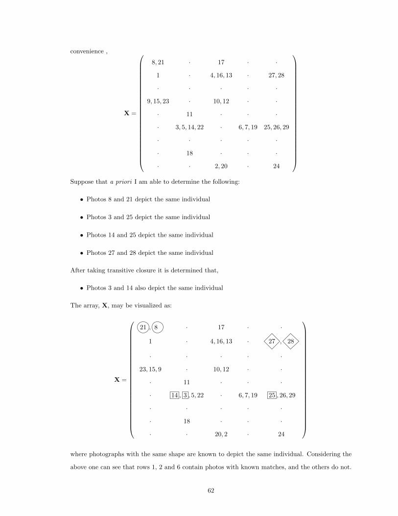
convenience ,

X =

8, 21 · 17 · ·

1 · 4, 16, 13 · 27, 28

· · · · ·

9, 15, 23 · 10, 12 · ·

· 11 · · ·

· 3, 5, 14, 22 · 6, 7, 19 25, 26, 29

· · · · ·

· 18 · · ·

· · 2, 20 · 24

Suppose that a priori I am able to determine the following:

• Photos 8 and 21 depict the same individual

• Photos 3 and 25 depict the same individual

• Photos 14 and 25 depict the same individual

• Photos 27 and 28 depict the same individual

After taking transitive closure it is determined that,

• Photos 3 and 14 also depict the same individual

The array, X, may be visualized as:

X =

21 , 80 · 17 · ·

1 · 4, 16, 13 · 27 , 28

· · · · ·

23, 15, 9 · 10, 12 · ·

· 11 · · ·

· 14 , 3 , 5, 22 · 6, 7, 19 25 , 26, 29

· · · · ·

· 18 · · ·

· · 20, 2 · 24

where photographs with the same shape are known to depict the same individual. Considering the

above one can see that rows 1, 2 and 6 contain photos with known matches, and the others do not.

62

Sampling from XY requires that when moving a photograph with a match restriction to a different

individual it is necessary to also move any photographs which are also known to depict the same

individual. Visually if a photograph is moved to a new individual them any photographs that share

the same shape must also be moved, IE no two rows can contain the same shape. Photographs

without match restrictions, such as photograph 11, are free to move to any individual.

Consider the second column of X. Notice that since I have determined photographs 3 and 14

depict the same individual then every element of XY will have those photographs placed in the

6th row since that individual is the only one photographed more than once in the second capture

occasion according to the given Y. Using only the restrictions listed above it can be shown that the

cardinality of XY is reduced from 181,440,000 to 1,935,360.

Case 3: Predetermined Matches and Non-Matches

When considering match restrictions and non-match restrictions simultaneously the process becomes

slightly more complicated. Similar to the case in which only match restrictions are considered, it will

be necessary to take transitive closure over the predetermined matches. However, it is also necessary

to form transitive closure over the predetermined non-matches. For example, if photographs A and

B are determined to not depict the same individual and photographs A and C are determined to

depict the same individual then Photographs A and C cannot depict the same individual, i.e. due to

transitive closure if C(X)j1,j2 = 1 and C(X)j1,j3 = 0 then C(X)j2,j3 = 0. There are cases in which

it is not possible to form transitive closure given some configurations of the predetermined matches

and non-matches, this issue is discussed in Section 3.2.3. I need to generate candidate X’s which

agree with the restrictions on XY . Once again provided for convenience is the previous realization

of X:

X =

8, 21 · 17 · ·

1 · 4, 13, 16 · 27, 28

· · · · ·

23, 15, 9 · 10, 12 · ·

· 11 · · ·

· 3, 5, 14, 22 · 6, 7, 19 25, 26, 29

· · · · ·

· 18 · · ·

· · 2, 20 · 24

63

Consider the combined information from the previous 2 cases:

• Photos 4 and 9 cannot depict the same individual

• Photos 1 and 23 cannot depict the same individual

• Photos 27 and 29 cannot depict the same individual

• Photos 8, and 21 depict the same individual

• Photos 3, 14 and 25 depict the same individual

• Photos 27 and 28 depict the same individual.

Taking transitive closure yields the additional information

• Photos 28 and 29 cannot depict the same individual.

The array, X , may be visualized as:

X =

80 , 21 · 17 · ·

1 · 4, 13, 16 · 27 , 28

· · · · ·

9, 15, 23 · 10, 12 · ·

· 11 · · ·

· 3 , 5, 14 , 22 · 6, 7, 19 25 , 26, 2929

· · · · ·

· 18 · · ·

· · 2, 20 · 24

where photographs with the same color denote photographs which are known not to depict the same

individual and photographs with the same shape denote photographs which are known to depict the

same individual. Using the above one can see that rows 1, 2, 3 and 5 contain photos with some kind

of restriction, and row 4 does not. Sampling from XY requires that when moving a photograph any

photographs which depict the same individual must also be moved while not violating a non-match

restriction. Visually one can see the complexity of even this small example. Considering the above

it is required that a color does not appear in a row more than once and also that a unique shape only

appears in a single row. By predetermining matches and non-matches there is a further reduction

in the cardinality of the restricted XY . Considering the restrictions listed above the cardinality of

XY is reduced from 181,440,000 to 1,447,110.

64

3.2.2 Fixing Elements of C(X) with Auxiliary Information

In the previous section I discussed the advantages of restricting the sample space of CY by fixing

some elements of C(X) but the discussion was void of which elements to fix. In this section I will

look at the choice of elements in C(X) to consider deterministic prior to fitting the model. I begin

by discussing how to incorporate auxiliary information then transition to the application of a record

linkage type rule to help make the choice.

In some experiments it may be possible to utilize auxiliary information to a priori determine

that 2 photographs do or do not depict the same individual. In the study of animals, auxiliary

information could include gender of the animal, family groups, time of photograph and location of

photograph. Auxiliary information can most easily be employed to determine non-matches. As an

example, in whale shark photography the gender of some individuals in the photographs is known

and for others it is not. If it is assumed that there is no misidentification of the gender of the animals

in the photographs then C(X)i,j = 0 when, photo i depicts a male and photo j depicts a female.

Other potentially beneficial auxiliary information that may be included are time and space. Another

example occurs if two photos are taken at the same time at different locations then the photographs

cannot depict the same individual. It may also be possible to employ known information about the

movement of whale sharks to define a maximum distance that the animals travel in a day to further

eliminate matches.

As a small example consider a set of 7 photographs. Photographs 1-2 are known to be male,

3-5 are known to be female and the gender is unknown for photographs 6-7. Using the auxiliary

information of gender C(X) is as follows:

C(X) =

1 C1,2 0 0 0 C1,6 C1,7

1 0 0 0 C2,6 C2,7

1 C3,4 C3,5 C3,6 C3,7

1 C4,5 C4,6 C4,7

1 C5,6 C5,7

1 C6,7

1

.

The application of auxiliary information aids in MCMC and specifically will aid in computa-

tion time. It may also reduce uncertainty in the model if auxiliary information is assumed to be

correct. One of the goals of the methods presented here is to eliminate the need for researchers to

65

examine every photograph. On the contrary in order for the gender of a photograph to be deter-

mined a researcher must examine the photo. Other auxiliary information can be gathered without

a researcher examining the photograph, for example time/location of photo. The application of

auxiliary information is highly recommended and should be used when feasible.

3.2.3 Application of Record Linkage Type Rule to Fix Elements of C(X)

The application of auxiliary information is a beneficial tool in predetermining matches and non-

matches, but in practice auxiliary information may be limited, unreliable or unavailable. Instead,

I propose to utilize the underlying distribution of the pairwise scores a priori to determine some

of the elements of C(X). Unlike the application of auxiliary information I know that there will be

some error. In order to fix some of the elements of C(X) a priori I developed an algorithm to aid

in identifying which elements of C(X) should be considered known. Similar to the record linkage

rule previously discussed the algorithm maps the pairs of photographs to one of three categories:

match, non-match and unknown based on the value of the corresponding pairwise score. The match

and non-match categories will place match and non-match restrictions on the sample space of C(X)

respectively. Pairs in the unknown category will be treated as possible matches and handled with the

methods described in Chapter 2. I begin by discussing the most complex portion of the algorithm

which defines the mapping to the match category.

It is desirable to identify as many match pairs as possible, since identification of match pairs

results in the largest reduction in the cardinality of the sample space. Ideally I would like to define a

cutoff, u, so that that any pairwise score greater than the cutoff value will be mapped to the match

category with only a small number of non-match scores greater than the cutoff. Recall that the

observed scores conditional on C(X) are regarded as draws from a mixture of known densities such

that

f(s|Ci,j(X)) = Ci,j(X)fm(s|ψm) + (1− Ci,j(X))fn(s|ψn)

for all i and j where ψm and ψn are the parameters of the density for matches and non-matches

respectively and ψ = (ψm, ψn) is known. Further let Fm(s|ψm) and Fn(s|ψn) to be the distribution

functions, matching the densities fm(s|ψm) and fn(s|ψn). One possible way to define u is to consider

the portion of the mixture distribution that the non-match scores arise from. I define an error rate

of αn, where αn equals the probability of observing a score greater than u given that the score is

non-match. Then u can be defined as the 1− αn quantile of the non-match portion of the mixture

distribution, i.e. u = F−1n (1− αn|ψn) .

66

As an example consider a single capture occasion study in which 20 photographs were taken.

Unknown to the researcher approximately 15% of the scores are generated from pairs of photographs

which are a match, i.e. they depict the same animal. A bar chart of a potential realization of the

data is depicted in Figure 3.1. Further suppose that it is known that the non-match scores originate

from a Be(2, 6) and the match scores originate from a Be(6, 2). Figure 3.1 illustrates the fitted

density curve of the observed scores.

Figure 3.1: The fitted density curve of the observed scores.

The goal is to identify with low error pairwise scores which were generated from a matching pair.

For this example set αn = .05 and u = F−1n (.95|ψn). Ignoring the observed scores momentarily one

67

may visualize what this means in terms of the two parts of the mixture distribution by viewing Figure

3.2 which depicts the mixture distribution with the upper 5 percent of the non-match distribution

shaded in blue. The proportion of the match scores that will be correctly identified when u =

F−1n (.95|ψn) is shaded in red. With an error of 5% placed in the upper tail of the non-match

distribution approximately 92% of the match scores are identified.

Figure 3.2: With an error of 5% placed in the upper tail of the non-match distribution I am able toidentify 92% of the match scores.

There is an issue with defining u = F−1n (1− αn|ψn). Even when the error rate is low it is likely

to identify a large number of true non-matches as matches since the majority of the pairwise scores

originate from photographs which do not depict the same individual. For example suppose the data

contain pairwise scores from 100 photographs where in truth all of the photographs depict a unique

individual. If αn = .05 then I will incorrectly identity approximately 248 of the 4,950 non-matching

pairs as match pairs by chance alone. This issue is further compounded when transitive closure is

taken over the identified matches. Even with an error rate of .05 or .01 it is possible after transitive

closure that the resulting C(X) places the majority of the photographs on a single individual. In

order to illustrate this issue consider the previous example where 20 photographs were taken on a

single capture occasion. Suppose unknown to the researcher that there are five individuals depicted

in the 20 photographs where the following sets of photographs depict 5 unique individuals: {1,5,6,8},

{2,3,7}, {4,9,10,13}, {11,12,14,18,19}, and {15,16,17,20}. Since the ordering of C(X) is arbitrary

68

I can order C(X) to match the ordering of the photographs above for convenience. Further since

C(X) is symmetric only the upper diagonal is needed and the matrix is as follows:

C(X) =

1 1 1 1 0 0 0 0 0 0 0 0 0 0 0 0 0 0 0 0 photo 1

1 1 1 0 0 0 0 0 0 0 0 0 0 0 0 0 0 0 0 photo 5

1 1 0 0 0 0 0 0 0 0 0 0 0 0 0 0 0 0 photo 6

1 0 0 0 0 0 0 0 0 0 0 0 0 0 0 0 0 photo 8

1 1 1 0 0 0 0 0 0 0 0 0 0 0 0 0 photo 2

1 1 0 0 0 0 0 0 0 0 0 0 0 0 0 photo 3

1 0 0 0 0 0 0 0 0 0 0 0 0 0 photo 7

1 1 1 1 0 0 0 0 0 0 0 0 0 photo 4

1 1 1 0 0 0 0 0 0 0 0 0 photo 9

1 1 0 0 0 0 0 0 0 0 0 photo 10

1 0 0 0 0 0 0 0 0 0 photo 13

1 1 1 1 1 0 0 0 0 photo 11

1 1 1 1 0 0 0 0 photo 12

1 1 1 0 0 0 0 photo 14

1 1 0 0 0 0 photo 18

1 0 0 0 0 photo 19

1 1 1 1 photo 15

1 1 1 photo 16

1 1 photo 17

1 photo 20

.

In this example there are 190 pairs of photographs to be compared, with 31 of the pairs representing

pairs of photographs that depict the same animal. Ordering the rows by the sets of photographs

creates a block diagonal matrix. Suppose that αn = .05, meaning that 5% of the true non-match

scores will be considered a match. In the above example there are 139 true non-match pairs and

approximately 8 of those pairs will produce scores higher than the cutoff when αn = .05. The

following matrix depicts a potential realization of non-match pairs that are incorrectly identified as

69

matches in red where the entries were chosen at random.

C(X) =

1 1 1 1 0 0 0 0 0 0 0 0 0 0 0 0 0 0 0 0 photo 1

1 1 1 0 0 0 0 0 0 0 0 0 0 0 0 0 0 0 0 photo 5

1 1 1 0 0 0 0 0 0 0 0 0 0 0 0 0 0 0 photo 6

1 0 0 0 1 0 0 0 0 0 0 1 0 0 0 0 0 photo 8

1 1 1 0 1 0 0 0 0 0 0 0 0 0 0 0 photo 2

1 1 0 0 0 0 0 1 0 0 0 0 0 0 0 photo 3

1 0 0 0 0 0 0 0 0 1 0 0 0 0 photo 7

1 1 1 1 0 0 0 0 0 0 0 0 0 photo 4

1 1 1 0 0 0 0 0 0 0 0 0 photo 9

1 1 0 0 0 0 0 0 0 0 0 photo 10

1 0 0 0 0 0 0 0 0 0 photo 13

1 1 1 1 1 1 0 0 0 photo 11

1 1 1 1 0 0 0 0 photo 12

1 1 1 0 0 0 0 photo 14

1 1 0 0 0 0 photo 18

1 0 1 0 0 photo 19

1 1 1 1 photo 15

1 1 1 photo 16

1 1 photo 17

1 photo 20

.

Recall that the properties of C(X) require that if photographs A and B depict the same individual,

and photographs A and C depict the same individual then photographs B and C must depict the

same individual. Considering the block diagonal format of the matrix, the false matches are depicted

as 1s in the blocks of zeros of the diagonal. These singletons then link all of the photographs in the

70

corresponding blocks which fills the entire matrix with 1s:

C(X) =

1 1 1 1 1 1 1 1 1 1 1 1 1 1 1 1 1 1 1 1 photo 1

1 1 1 1 1 1 1 1 1 1 1 1 1 1 1 1 1 1 1 photo 5

1 1 1 1 1 1 1 1 1 1 1 1 1 1 1 1 1 1 photo 6

1 1 1 1 1 1 1 1 1 1 1 1 1 1 1 1 1 photo 8

1 1 1 1 1 1 1 1 1 1 1 1 1 1 1 1 photo 2

1 1 1 1 1 1 1 1 1 1 1 1 1 1 1 photo 3

1 1 1 1 1 1 1 1 1 1 1 1 1 1 photo 7

1 1 1 1 1 1 1 1 1 1 1 1 1 photo 4

1 1 1 1 1 1 1 1 1 1 1 1 photo 9

1 1 1 1 1 1 1 1 1 1 1 photo 10

1 1 1 1 1 1 1 1 1 1 photo 13

1 1 1 1 1 1 1 1 1 photo 11

1 1 1 1 1 1 1 1 photo 12

1 1 1 1 1 1 1 photo 14

1 1 1 1 1 1 photo 18

1 1 1 1 1 photo 19

1 1 1 1 photo 15

1 1 1 photo 16

1 1 photo 17

1 photo 20

.

Examining the matrix all of the true non-matches are now matches. In this small example by

setting an αn = .05 error rate on the non-match scores all of the photographs are mapped to a single

individual. There is nothing remarkable about this particular example, the same behavior can be

seen in much larger sets of photographs and can occur with error rates much smaller than .05.

In order to address this issue I propose an algorithm which incorporates two cutoff values, we will

refer to them as u1 and u2, where u1 > u2 . The purpose of the first cutoff, u1, is to identify as many

true matches as possible while mislabeling non-matches as matches at a rate close to zero. Pairs of

photographs with scores greater than u1 will be considered a match. This can be accomplished by

setting u1 = F−1n (1 − αn1)|ψn) where αn1 is extremely small, or so that F−1n (1 − αn1)|ψn) is the

maximum known non-match score from the training data. The appropriate size of αn1will depend

71

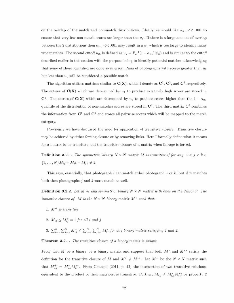
on the overlap of the match and non-match distributions. Ideally we would like αn1 << .001 to

ensure that very few non-match scores are larger than the u1. If there is a large amount of overlap

between the 2 distributions then αn1<< .001 may result in a u1 which is too large to identify many

true matches. The second cutoff u2, is defined as u2 = F−1n (1−αn2)|ψn) and is similar to the cutoff

described earlier in this section with the purpose being to identify potential matches acknowledging

that some of those identified are done so in error. Pairs of photographs with scores greater than u2

but less than u1 will be considered a possible match.

The algorithm utilizes matrices similar to C(X), which I denote as C1, C2, and C3 respectively.

The entries of C(X) which are determined by u1 to produce extremely high scores are stored in

C1. The entries of C(X) which are determined by u2 to produce scores higher than the 1 − αn2

quantile of the distribution of non-matches scores are stored in C2. The third matrix C3 combines

the information from C1 and C2 and stores all pairwise scores which will be mapped to the match

category.

Previously we have discussed the need for application of transitive closure. Transitive closure

may be achieved by either forcing closure or by removing links. Here I formally define what it means

for a matrix to be transitive and the transitive closure of a matrix when linkage is forced.

Definition 3.2.1. The symmetric, binary N × N matrix M is transitive if for any i < j < k ∈

{1, . . . , N}Mij +Mik +Mjk 6= 2.

This says, essentially, that photograph i can match either photograph j or k, but if it matches

both then photographs j and k must match as well.

Definition 3.2.2. Let M be any symmetric, binary N ×N matrix with ones on the diagonal. The

transitive closure of M is the N ×N binary matrix M+ such that:

1. M+ is transitive

2. Mij ≤M+ij = 1 for all i and j

3.∑Ni=1

∑Nj=1M

+ij ≤

∑Ni=1

∑Nj=1M

∗ij for any binary matrix satisfying 1 and 2.

Theorem 3.2.1. The transitive closure of a binary matrix is unique.

Proof. Let M be a binary be a binary matrix and suppose that both M∗ and M∗∗ satisfy the

definition for the transitive closure of M and M∗ 6= M∗∗. Let M+ be the N × N matrix such

that M+i,j = M∗i,jM

∗∗i,j . From Chuaqui (2011, p. 42) the intersection of two transitive relations,

equivalent to the product of their matrices, is transitive. Further, Mi,j ≤ M∗i,jM∗∗i,j by property 2

72

above and∑Ni=1

∑Nj=1M

+ij ≤

∑Ni=1

∑Nj=1M

∗ij and

∑Ni=1

∑Nj=1M

+ij ≤

∑Ni=1

∑Nj=1M

∗∗ij with one of

these inequalities being strict. This means that either M∗ or M∗∗ doesn’t satisfy the summation

property. This is a contradiction and shows that transitive closure is unique.

Next I outline the algorithm which identifies sets of matching photographs.

1. Identify and store matches with low/no error

i) Set C1 = INp .

ii) Set u1 = F−1n (1− αn1)|ψn).

iii) For all i, j such that Si,j > u1 set C1i,j=1 and C1

j,i=1.

iv) Compute C1+.

v) Let V1 be a collection of sets, J1, . . . ,Jnj where nj ≤ Np, which partition the rows of

C1+. Where Jl contains the rows of C1+ corresponding the lth set of photographs which

depict the same individual identified by u1, where l = 1, . . . , nj .

vi) Set C3 = C1+.

2. Identify and store potential match scores.

i) Set C2 = INp .

ii) Set u2 = F−1n (1− αn2)|ψn) where αn2 is the desired error rate.

iii) For all i, j such that Si,j > u2 set C2i,j=1 and C2

j,i=1.

3. Compare potential matches to the previously identified matches.

i) For i = 1, . . . , nj .

If #Ji > 1:

– Let bi =∑j∈Ji C2

j,{1,...,Np}.

– Let Gi be the set of g such that big = #Ji.

– Let di =∑g∈Gi C2

g,{1,...,Np}.

– let Ki be a subset of Gi corresponding to the elements of d = #Gi.

– For all k and k′ in Ki set C3k,k′ = 1.

ii) Compute C3+.

4. Build the Match Sets

73

i) Let V2 be a collection of sets, M1, . . . ,Mnm where nm ≤ Np, which partition the rows

of C3+. Where Ml contains the rows of C3+ corresponding the lth set of photographs

which depict the same individual, where l = 1, . . . , nm.

ii) Sort the setsM1, . . . ,Mnm from largest to smallest by cardinality and within cardinality

are ordered by smallest element.

I will continue the earlier example and illustrate each step of the algorithm. Previously the matrix

was ordered based on the true match nature of the photographs to motivate the need for the match-

ing algorithm. Here the matrix is not ordered based on the true match/non-match nature of the

photographs. Instead I order the photographs by ID and the row number of C corresponds to the

ID of the photograph to illustrate the that algorithm does not depend on knowing the true nature

of the photographs.

1. Identify and store matches with low/no error.

Begin by setting C1 = I20. Suppose that S1,6, S2,3, S4,9, S6,8, S10,13, S11,12, S12,18, S15,16,

74

S15,17 and S18,19 are all greater than u1. After computing C1+ I have the following:

C1+ =

1 0 0 0 0 1 0 1 0 0 0 0 0 0 0 0 0 0 0 0

1 1 0 0 0 0 0 0 0 0 0 0 0 0 0 0 0 0 0

1 0 0 0 0 0 0 0 0 0 0 0 0 0 0 0 0 0

1 0 0 0 0 1 0 0 0 0 0 0 0 0 0 0 0

1 0 0 0 0 0 0 0 0 0 0 0 0 0 0 0

1 0 1 0 0 0 0 0 0 0 0 0 0 0 0

1 0 0 0 0 0 0 0 0 0 0 0 0 0

1 0 0 0 0 0 0 0 0 0 0 0 0

1 0 0 0 0 0 0 0 0 0 0 0

1 0 0 1 0 0 0 0 0 0 0

1 1 0 0 0 0 0 1 1 0

1 0 0 0 0 0 1 1 0

1 0 0 0 0 0 0 0

1 0 0 0 0 0 0

1 1 1 0 0 0

1 1 0 0 0

1 0 0 0

1 1 0

1 0

1

.

Next identify the collection V1. Notice that the unique rows of C1+ inform which sets of

photographs depict the same individual. Each Jl ∈ V1, l = 1, . . . , nj represents a set of

photographs depicting the same individual. For example notice that rows 1, 6, and 8 of C1+

are identical therefore photographs 1, 5 and 8 comprise one of the Jl ∈ V1. The ordering of

Jl ∈ V1 is arbitrary and V1 is as follows:

V1 = {{1, 6, 8}, {2, 3}, {4, 9}, {5}, {7}, {10, 13}, {11, 12, 18, 19}, {14}, {15, 16, 17}, {20}}.

Examining V1 there are nj = 10 distinct sets of photographs, where the photographs in each

set depict the same individual. Further 6 of the sets contain more than 1 photograph. It

75

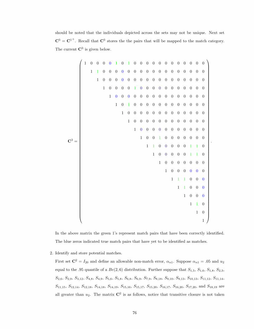
should be noted that the individuals depicted across the sets may not be unique. Next set

C3 = C1+. Recall that C3 stores the the pairs that will be mapped to the match category.

The current C3 is given below.

C3 =

1 0 0 0 0 1 0 1 0 0 0 0 0 0 0 0 0 0 0 0

1 1 0 0 0 0 0 0 0 0 0 0 0 0 0 0 0 0 0

1 0 0 0 0 0 0 0 0 0 0 0 0 0 0 0 0 0

1 0 0 0 0 1 0 0 0 0 0 0 0 0 0 0 0

1 0 0 0 0 0 0 0 0 0 0 0 0 0 0 0

1 0 1 0 0 0 0 0 0 0 0 0 0 0 0

1 0 0 0 0 0 0 0 0 0 0 0 0 0

1 0 0 0 0 0 0 0 0 0 0 0 0

1 0 0 0 0 0 0 0 0 0 0 0

1 0 0 1 0 0 0 0 0 0 0

1 1 0 0 0 0 0 1 1 0

1 0 0 0 0 0 1 1 0

1 0 0 0 0 0 0 0

1 0 0 0 0 0 0

1 1 1 0 0 0

1 1 0 0 0

1 0 0 0

1 1 0

1 0

1

.

In the above matrix the green 1’s represent match pairs that have been correctly identified.

The blue zeros indicated true match pairs that have yet to be identified as matches.

2. Identify and store potential matches.

First set C2 = I20 and define an allowable non-match error, αn1. Suppose αn1 = .05 and u2

equal to the .95 quantile of a Be(2, 6) distribution. Further suppose that S1,5, S1,6, S1,8, S2,3,

S2,6, S2,9, S3,12, S4,8, S4,9, S5,6, S5,8, S6,8, S6,9, S7,9, S8,18, S9,10, S9,13, S10,13, S11,12, S11,14,

S11,15, S12,14, S12,18, S14,18, S14,19, S15,16, S15,17, S15,20, S16,17, S16,20, S17,20, and S18,19 are

all greater than u2. The matrix C2 is as follows, notice that transitive closure is not taken

76

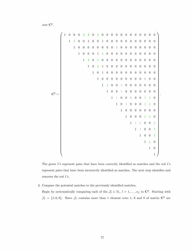
over C2.

C2 =

1 0 0 0 1 1 0 1 0 0 0 0 0 0 0 0 0 0 0 0

1 1 0 0 1 0 0 1 0 0 0 0 0 0 0 0 0 0 0

1 0 0 0 0 0 0 0 0 1 0 0 0 0 0 0 0 0

1 0 0 0 1 1 0 0 0 0 0 0 0 0 0 0 0

1 1 0 1 0 0 0 0 0 0 0 0 0 0 0 0

1 0 1 1 0 0 0 0 0 0 0 0 0 0 0

1 0 1 0 0 0 0 0 0 0 0 0 0 0

1 0 0 0 0 0 0 0 0 0 1 0 0

1 1 0 0 1 0 0 0 0 0 0 0

1 0 0 1 0 0 0 0 0 0 0

1 1 0 0 1 0 0 1 1 0

1 0 1 0 0 0 1 1 0

1 0 0 0 0 0 0 0

1 0 0 0 1 1 0

1 1 1 0 0 1

1 1 0 0 1

1 0 0 1

1 1 0

1 0

1

.

The green 1’s represent pairs that have been correctly identified as matches and the red 1’s

represent pairs that have been incorrectly identified as matches. The next step identifies and

removes the red 1’s.

3. Compare the potential matches to the previously identified matches.

Begin by systematically comparing each of the Jl ∈ V1, l = 1, . . . , nj to C2. Starting with

J1 = {1, 6, 8}. Since J1 contains more than 1 element rows 1, 6 and 8 of matrix C2 are

77

examined. Resulting in:

C2{1,6,8}, =

1 0 0 0 1 1 0 1 0 0 0 0 0 0 0 0 0 0 0 0

1 0 0 0 1 1 0 1 1 0 0 0 0 0 0 0 0 0 0 0

1 0 0 0 1 1 0 1 0 0 0 0 0 0 0 0 0 1 0 0

.

Summing over the columns:

b1 =

(3 0 0 0 3 3 0 3 1 0 0 0 0 0 0 0 0 1 0 0

).

Since columns 1, 5, 6, and 8 have sum equal to the number of elements in J1 they belong

to a potential match set and let G1 to be the set comprised of {1, 5, 6, 8}. Next compare the

photographs to one another by examining C2{1,5,6,8},{1,5,6,8}. Resulting in:

C2{1,5,6,8},{1,5,6,8} =

1 1 1 1

1 1 1 1

1 1 1 1

1 1 1 1

.

Summing over the columns:

d1 =

(4 4 4 4

).

Since all of the column sums equal to #Gi, we have Ki = {1, 5, 6, 8}. For each k and k′ in

{1, 5, 6, 8} we set C3k,k′ = 1. Once the above has been completed for all Jl ∈ V1, l = 1, . . . , nj

78

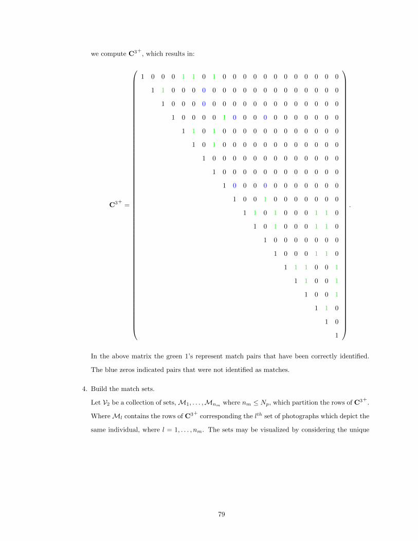
we compute C3+, which results in:

C3+ =

1 0 0 0 1 1 0 1 0 0 0 0 0 0 0 0 0 0 0 0

1 1 0 0 0 0 0 0 0 0 0 0 0 0 0 0 0 0 0

1 0 0 0 0 0 0 0 0 0 0 0 0 0 0 0 0 0

1 0 0 0 0 1 0 0 0 0 0 0 0 0 0 0 0

1 1 0 1 0 0 0 0 0 0 0 0 0 0 0 0

1 0 1 0 0 0 0 0 0 0 0 0 0 0 0

1 0 0 0 0 0 0 0 0 0 0 0 0 0

1 0 0 0 0 0 0 0 0 0 0 0 0

1 0 0 0 0 0 0 0 0 0 0 0

1 0 0 1 0 0 0 0 0 0 0

1 1 0 1 0 0 0 1 1 0

1 0 1 0 0 0 1 1 0

1 0 0 0 0 0 0 0

1 0 0 0 1 1 0

1 1 1 0 0 1

1 1 0 0 1

1 0 0 1

1 1 0

1 0

1

.

In the above matrix the green 1’s represent match pairs that have been correctly identified.

The blue zeros indicated pairs that were not identified as matches.

4. Build the match sets.

Let V2 be a collection of sets,M1, . . . ,Mnm where nm ≤ Np, which partition the rows of C3+.

WhereMl contains the rows of C3+ corresponding the lth set of photographs which depict the

same individual, where l = 1, . . . , nm. The sets may be visualized by considering the unique

79

rows of C3+. The unique rows are as follows:

1 0 0 0 1 1 0 1 0 0 0 0 0 0 0 0 0 0 0 0

0 1 1 0 0 0 0 0 0 0 0 0 0 0 0 0 0 0 0 0

0 0 0 1 0 0 0 0 1 0 0 0 0 0 0 0 0 0 0 0

0 0 0 0 0 0 1 0 0 0 0 0 0 0 0 0 0 0 0 0

0 0 0 0 0 0 0 0 0 1 0 0 1 0 0 0 0 0 0 0

0 0 0 0 0 0 0 0 0 0 1 1 0 1 0 0 0 1 1 0

0 0 0 0 0 0 0 0 0 0 0 0 0 0 1 1 1 0 0 1

.

Notice that C3+ has 7 unique rows therefore nm = 7 resulting in:

V2 = {{1, 5, 6, 8}, {2, 3}, {4, 9}, {7}, {10, 13}, {11, 12, 14, 18, 19}, {15, 16, 17, 20}}

As a last step the sets are organized from smallest to largest, resulting in the following match

sets:

{11, 12, 14, 18, 19}

{1, 5, 6, 8}

{15, 16, 17, 20}

{2, 3}

{4, 9}

{10, 13}

{7}

Once the pairs to map to the match category have been identified attention is moved to which pairs

should be mapped to the non-match category. Similar to the match score scenario a cutoff value, l, is

defined so that any pairwise score lower than the cutoff will be mapped to the non-match category.

Ideally I would like to define l so that only a small number of match scores are lower than the

cutoff. Once again recall that the observed scores conditional on C(X) are regarded as draws from

a mixture of known densities such that

f(s|Ci,j(X)) = Ci,j(X)fm(s|ψm) + (1− Ci,j(X))fn(s|ψn)

80

for all i and j where ψm and ψn are the parameters of the density for matches and non-matches

respectively and ψ = (ψm, ψn) is known. Further let Fm(s|ψm) and Fn(s|ψn) to be the distribution

functions, matching the densities fm(s|ψm) and fn(s|ψn). One possible way to define a cutoff, l,

is to consider the portion of the mixture distribution from which the match scores arise from and

define an error rate of αm, where αm equals the probability of observing a score lower than l given

that the score is a match. Then the cutoff can be defined as the αm quantile of the match portion

of the mixture distribution or l = F−1m (αm|ψm).

As an example consider the beta mixture discussed in Chapter 2 where the non-matches scores

originate from a Be(2, 6) and the match scores originate from a Be(6, 2). Further suppose that we

wish to set αm = .05. Figure 3.3 depicts the mixture distribution with the lower 5 percent of the

match distribution shaded in red. The proportion of the non-match scores which will be correctly

identified using the .05 quantile of the non-match distribution as a cutoff is shaded in blue.

Figure 3.3: With an error of 5% placed in the lower tail of the match distribution 92% of thenon-match scores are identified.

Unlike the match case there is not an issue with defining the cutoff as F−1m (αm|ψm). There are

two reasons why defining the cutoff in this manor does not cause the same issues as the match case.

Since typically majority of the pairwise scores originate from pairs of photographs which do not

81

depict the same individual we do not have many pairwise scores that originate from true matches.

Further by completing the mapping to the match category first some scores lower than l will have

already been identified as matches as a result of transitive closure. Those scores previously mapped

to the match category will maintain their status.

Below is an outline of the algorithm for mapping scores to the non-match category. When the

algorithm is utilized in conjunction with the Score Based Mark-Recapture model I will refer to it as

the Fast Score Based Mark-Recapture model.

1. Identify and store potential non-matches.

i) Set C4 = 0Np,Np .

ii) Set l = F−1m (αm|ψm).

iii) For all i, j such that Si,j < l set C4i,j=1 and C4

j,i=1.

2. If photographs A and B are non-match and photographs A and C are matches then transitivity

requires that photographs C and A be non-matches, see Definition 3.2.1.

i) For i = 1, . . . , nm.

- Let wi =∑m∈Mi

C2m,{1,...,Np}.

- Let Hi be the set of h such that wih > 0.

- For each i ∈Mi and j ∈ Hi set C4ij = 1 and C4

ji = 1.

3. Build the non-match sets.

i) Let V3 be a collection of sets, N1, . . .NNp .

ii) For i = 1, . . . , Np.

- Let Ni be the set of j such that C4i,j=1.

4. Compare the non-match sets to the match sets and remove contradictions.

i) For i = 1, . . . , nm.

For j = 1, . . . ,#Ni.

- Let k equal to the jth element of Mi.

- Let Rij be the set elements of Mi ∈ Nk.

- Remove the elements of Rij from Nk.

82

As an example consider the previously discussed set of 20 photographs. Illustrated here is each step

of the algorithm.

1. Identify and store potential non-matches.

Begin by setting C4 to be a 20 × 20 zero matrix. Suppose that S1,8, S1,11, S1,12, S2,4, S2,6,

S2,9, S2,17, S3,5, S3,6, S3,20, S4,5, S4,15, S4,16, S5,7, S5,10, S5,13, S6,11, S6,12, S6,17, S7,9, S7,16,

S8,9, S8,13, S9,11, S9,16, S9,17, S10,11, S10,20, S11,13, S12,15, S13,16, S13,17, S14,17, S16,18, and

S19,20 are all less than l. The matrix C4 is as follows,

C4 =

0 0 0 0 0 0 0 1 0 0 1 1 0 0 0 0 0 0 0 0

0 0 1 0 1 0 0 1 0 0 0 0 0 0 0 1 0 0 0

0 0 1 1 0 0 0 0 0 0 0 0 0 0 0 0 0 1

0 1 0 0 0 0 0 0 0 0 0 1 1 0 0 0 0

0 0 1 0 0 1 0 0 1 0 0 0 0 0 0 0

0 0 0 0 0 1 1 0 0 0 0 1 0 0 0

0 0 1 0 0 0 0 0 0 1 0 0 0 0

0 1 0 0 0 1 0 0 0 0 0 0 0

0 0 1 0 0 0 0 1 1 0 0 0

0 1 0 0 0 0 0 0 0 0 1

0 0 1 0 0 0 0 0 0 0

0 0 0 1 0 0 0 0 0

0 0 0 1 1 0 0 0

0 0 0 1 0 0 0

0 0 0 0 0 0

0 0 1 0 0

0 0 0 0

0 0 0

0 1

0

.

2. If photographs A and B are non-matches and photographs A and C are matches then transi-

tivity requires that photographs C and A be non-matches.

This step will compare each of the match sets to C4. As an example the second match set

contains the photos {1, 5, 6, 8}. Next consider rows 1, 5, 6 and 8 of C4 and sum over the

83

columns. This will inform all of the photographs which have a non-match restriction with any

photograph in the second match set. Summing over the columns we have:

w2 =

(1 1 2 1 0 0 1 1 1 1 2 2 1 0 0 0 1 0 0 0

).

Then:

H2 = {1, 2, 3, 4, 7, 8, 9, 10, 11, 12, 13, 17}

All of the photographs in H2 have a non-match restriction against at least one photograph

in the second match set therefore all photographs in the second match set have non-match

restriction with all photographs in H2. This information in reflected in C4 by setting C4ij = 1

and C4ji = 1 for each i ∈ {1, 5, 6, 8} and j ∈ {1, 2, 3, 4, 7, 8, 9, 10, 11, 12, 13, 17}. After the

84

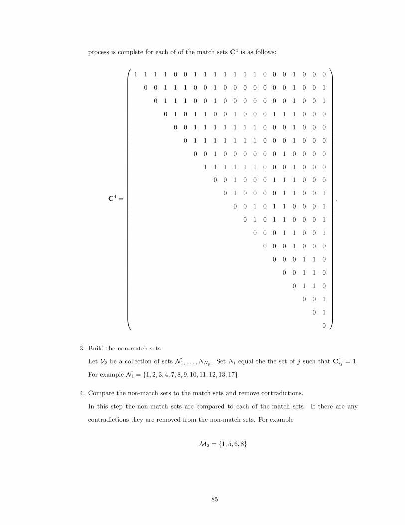
process is complete for each of of the match sets C4 is as follows:

C4 =

1 1 1 1 0 0 1 1 1 1 1 1 1 0 0 0 1 0 0 0

0 0 1 1 1 0 0 1 0 0 0 0 0 0 0 1 0 0 1

0 1 1 1 0 0 1 0 0 0 0 0 0 0 1 0 0 1

0 1 0 1 1 0 0 1 0 0 0 1 1 1 0 0 0

0 0 1 1 1 1 1 1 1 0 0 0 1 0 0 0

0 1 1 1 1 1 1 1 0 0 0 1 0 0 0

0 0 1 0 0 0 0 0 0 1 0 0 0 0

1 1 1 1 1 1 0 0 0 1 0 0 0

0 0 1 0 0 0 1 1 1 0 0 0

0 1 0 0 0 0 1 1 0 0 1

0 0 1 0 1 1 0 0 0 1

0 1 0 1 1 0 0 0 1

0 0 0 1 1 0 0 1

0 0 0 1 0 0 0

0 0 0 1 1 0

0 0 1 1 0

0 1 1 0

0 0 1

0 1

0

.

3. Build the non-match sets.

Let V2 be a collection of sets N1, . . . , NNp . Set Ni equal the the set of j such that C4ij = 1.

For example N1 = {1, 2, 3, 4, 7, 8, 9, 10, 11, 12, 13, 17}.

4. Compare the non-match sets to the match sets and remove contradictions.

In this step the non-match sets are compared to each of the match sets. If there are any

contradictions they are removed from the non-match sets. For example

M2 = {1, 5, 6, 8}

85

and

N1 = {1, 2, 3, 4, 7, 8, 9, 10, 11, 12, 13, 17}.

The N1 suggest that the photographs 1, 5, 6 and 8 do not match photos 1 and 8, therefore

R11 = {1, 8}. This is an obvious contradiction so photos 1 and 8 are removed from N1.

3.2.4 MCMC Sampling

In previous sections the advantages of restricting the sample space of CY by fixing some elements of

C(X) as well as the choice of which elements to consider fixed were discussed. Unfortunately the

custom sampler presented in Chapter 2 cannot sample the restricted sample space of CY . Movement

around the restricted sample space is much more complex as illustrated in Section 3.2. Provided are

details on a new custom sampler, which can handle the restrictions on the sample space of CY , fitting

the CMSA formulation of the JS model (Crosbie and Manly, 1985; Schwarz and Arnason, 1996) as

the underlying mark-recapture model. The update of p, φ and β have been well documented in

other texts, such as Link and Barker (2009, Chapter 11), and details were provided in Chapter 2.

3.2.5 Adding or Deleting an Individual with Dependencies

The update of adding or deleting an individual is the most complicated type of update because the

addition of a new individual requires sampling new times of birth, death, a new capture history and

to movement of photographs between the individuals (if the newly generated individual is captured

at least once). Let W′,Y′,X′, b′ and d′ denote the candidate W,X,Y, b and d respectively. To

create the candidates it is randomly decided to add a new individual with probability q or delete an

individual with probability 1− q. By default q = .5. Provided below is an outline of the process of

generating the candidates once the choice to add or delete an individual is made.

• Adding a new individual

Data for a new individual in the population is simulated in the following steps:

1. Generate an ID for the new individual:

Simulate j ∼ Uniform(1, . . . , N + 1).

2. Generate capture information for the new individual:

i) Simulate b′j |β.

ii) Simulate d′j |b′j ,φ.

iii) For t = 1, . . . , T ;

86

If t < b′j or t > d′j set w′j,t = 0 and Y ′j,t = 0.

Else,

a) Simulate w′j,t ∼ Bernoulli(pt).

b) If wj,t = 0 set Y ′j,t = 0. Otherwise generate Y ′j,t ∼ ZTPoisson(λ).

3. Generate photographs for the new individual:

i) Set Y ′j1, .., Y′jT = 0.

ii) Set Sj = ∅.

iii) Set k=1.

a) Set zkt equal to the number of photographs in the Mk taken on occasion t =

1, . . . , T .

b) If zkt ≤ Y ′j1 − Y ′j1 for all t = 1, . . . , T and match set k does not share elements

with S:

- Add match set k to the new individual with probability pk.

- Update S by adding the non-match sets associated with match set k to S.

- Set Y ′jt = zkt + Y ′jt for all t = 1, . . . , T .

4. Set k = k + 1 and repeat step 3 until either:

i) Y ′j1 − Y ′j1 = 0 for all t = 1, . . . , T .

ii) k = K and Y ′j1− Y ′j1 > 0 for some t = 1, . . . , T , where K is the number of match sets.

5. Create X′, b′, and d′:

i) If Y ′j,t > 0 let v be a vector of length Y ′j,t containing the ID of each photograph added

in the previous steps.

ii) Set X′ = X.

iii) For l = 1, . . . , Np

If X[l, 2] < j, set X′[l, 2] = X[l, 2]

Else set X′[l, 2] = X[l, 2] + 1

iv) Set X′[v, 2] = j.

v) Set b′ = (b1, . . . , bj−1, b′j , bj , . . . , bN ).

vi) Set d′ = (d1, . . . , dj−1, d′j , dj , . . . , dN ).

• Deleting an individual

87

1. Select an individual ID to delete:

Simulate j ∼ Uniform(1, . . . , N).

2. Create X′, b′, and d′:

i) Set X′ = X

ii) For l = 1, . . . , Np

If X[l, 2] < j, set X′[l, 2] = X[l, 2]

Else set X′[l, 2] = X[l, 2]− 1

iii) Set b′ = (b1, . . . , bj−1, bj+1, . . . , bN ).

iv) Set d′ = (d1, . . . , dj−1, dj+1, . . . , dN ).

v) For k = 1, . . . ,K, where K is the number of match sets, belonging to individual j.

a) Let Pk be the vector of p such that X[p,2]=j and photograph p is in the kth match

set.

b) Let Ak be the vector of i such that bi ≤ X[p, 1] and di ≥ X[p, 1] for all p ∈ Pk.

c) Let Rk be the vector of all photographs in non-match sets corresponding to

p ∈ Pk.

d) If X[r, 2] = i remove i from Ak.

e) Generate X[Pk, 2] ∼ Uniform(A).

Although Markov chains previously defined will converge to the proper distribution, I recommend

three additional updates to aid in mixing. The mixing steps are outlined in Section 2.3.7.

3.3 Application

Provided in this section are the results from application to data from whaleshark.org and simulated

data. The results will be compared to the results from Chapter 2. As mentioned previously when

the algorithm for determining fixed matches and non-matches are applied to the Score Based Mark-

Recapture model I will denote it as the Fast Score Based Mark-Recapture Model.

3.3.1 Simulated Data

To assess the performance of the Fast Score Based Mark-Recapture model I conducted a simulation

study. The primary objective was to compare the results of the Score Based Mark-Recapture model

and the Fast Score Based Mark-Recapture model as well as to determine how the performance was

affected by the overlap in the distributions for the match and non-match scores. Previously in

88

Chapter 2 it was seen that the Score Based Mark-Recapture model performed well when λ = 3 for

different beta mixtures. To assess the Fast Score Based Mark-Recapture model data was simulated

under the CMSA formulation of the JS model with T = 5, N = 200, β = (.6, .1, .1, .1, .1), φt = .8

and pt = .5. These values were chosen because they represent a species that has high survival

probability and moderate capture probability similar to the whale sharks. Scores were simulated

from three different beta mixtures, with each mixture having different amount of overlap between

the match and non-match portion of the mixture.

For each set of parameters 100 data sets were simulated, both the Score Based Mark-Recapture

model and the Fast Score Based Mark-Recapture model were fit utilizing MCMC with 50,000 burn in

and 50,000 sampling iterations. Further within each set the data for each of the different models was

the same and the chains were started at the same initial value. By considering both the Score Based

Mark-Recapture model and the Fast Score Based Mark-Recapture model I was able to compare

the coverage and width of credible intervals with and without a priori fixing elements. Further the

posterior mean was evaluated as a point estimate, N , for N by computing the percent bias. The

formula for the percent bias is given by:

100× N −NN

Table 3.1 summarizes the results from the simulation of credible intervals for population size. I

found that for each of the sets the the Score Based Mark-Recapture model and the Fast Score Based

Mark-Recapture model both produced credible intervals that have similar coverage and width.

Table 3.1: The first column list the value of α for the Beta distribution of match scores and thevalue β for the non-match scores. For each simulation the value of α for the Beta distributionof non-match scores and the value β for the match scores was equal to 2. The second columnlist the method, either the Score Based Mark-Recapture model (SB) or the Fast Score BasedMark-Recapture model (FSB). The fourth column denotes the percentage of overlap between thematch and non-match distributions. The fifth column denotes the percent coverage of the parameterN for 100 credible intervals. The fourth column lists the mean interval width. The last columngives the percent bias for the posterior mean as a point estimate for N = 200.

(αm, βn) (αn, βm) % Overlap Method % Coverage Mean CI Width % Bias8 2 3.9 S.B. 97 63.9 .11

F.S.B. 94 62.8 -.486 2 12.5 S.B. 92 64.9 .46

F.S.B. 92 65.8 .034 2 37.5 S.B. 93 63.6 -1.02

F.S.B. 92 61.3 -2.39

89

The Fast Score Based Mark-Recapture model produced similar results to the Score Based Mark-

Recapture model and ran in less time. As an example consider the first set of chains. Provided in

Table 3.2 are the elapsed system times for the first set chains of length 100,000 for both the Score

Based Mark-Recapture model and the Fast Score Based Mark-Recapture model under three Beta

mixtures. Examining the table I can see that for each of the set the Fast Score Based Mark-Recapture

model ran in less time. Further as the overlapping area between the mixture of betas increases the

run time for the Fast Score Based Mark-Recapture model decreases while the run time for the Score

Based Mark-Recapture model does not exhibit much change. This result is not surprising because

as the overlap between the distribution decreases the algorithm described in Chapter 3 is able to

identify more pairs as matches or non-matches resulting in a lower run time.

Table 3.2: The first and second column give the value of α for the Beta distribution of match scoresand the value β for the non-match scores respectively. The third column gives the percent overlapbetween the match and non-match distributions. The fourth and fifth column give the elapsedsystem time in hours for 100,000 iterations of the Score Based Mark-Recapture model (S.B.) andthe Fast Score Based Mark-Recapture model (F.S.B.) respectively.

(αm, βn) (αn, βm) % Overlap Elapsed Time S.B. Elapsed Time F.S.B.8 2 3.9 2.5 1.66 2 12.5 2.6 1.94 2 37.5 2.5 2.2

3.3.2 Whale Shark Data Set

Recall from Chapter 2 the data comprise pairwise scores from 820 photographs taken of whale sharks

(Rhincodon typus) in the northern ecotourism zone of the Nigaloo Marine Park near Exmouth on

the North West Cape of Australia (21◦ 55’59S 114◦ 7’41E) and submitted to whaleshark.org between

2003 and 2008. Whale sharks are the worlds largest fish and possess unique spot patterns located

on the side of the animals which make photo identification of the animals possible (Holmberg et al.,

2008). Previously I fit the Score Based Mark-Recapture model from Chapter 2 considering the

pairwise scores as data and the CMSA model considering the true match/non-match status of the

photographs as data.

Additionally recall from Section 2.2.1 that I regard the observed scores conditional on C(X) as

draws from a mixture of known densities such that

f(s|Ci,j(X)) = Ci,j(X)fm(s|ψm) + (1− Ci,j(X))fn(s|ψn)

90

for all i and j where ψm and ψn are the parameters of the density for matches and non-matches

respectively and ψ = (ψm, ψn) is known. Next I formulate the distribution for the match scores,

noting that the distribution for the non-match scores has similar form. One important aspect of the

data from the whale shark study contains a large number of zero scores, for both non-matches and

matches, which are associated with early termination of the scoring algorithm. To accommodate

this, I employ a further mixture distribution providing point mass at 0. The exact formulation is:

f(si,j |ψm, θm) =

I{si,j = 0}θm + (1− I{si,j = 0})(1− θm)g(si,j |ψm).

where g(si,j |ψm) is the density of scores greater than 0 and θm is the probability of observing a zero

score given that the two photographs are a match.

In the case of the modified Groth scores from the whale shark data I found that the non-zero scores

could be adequately modeled as normally distributed after applying the Box-Cox transformation so

that

g(si,j |ψm) = φ(h(si,j)− µm

σm

)sλm−1i,j

where φ(·) represents the density of the standard normal and ψm = (λm, σm, µm) and

h(Si,j)|Ci,j·∼ N(µm, σ

2m)

where h(Si,j)|Ci,j =sλmi,j −1λm

.

Recall that a score of zero is assigned to a pair of photographs when the matching algorithm

is unable to compute a score and terminates. These cases will be referred to as terminations. In

order to a priori determine match and non-match scores only the scores from the whale shark data

set which were not terminations will be examined. The algorithm discussed in Section 3.2.2 is

not able to directly handle the terminations but will be able to set some pairs of photographs for

which the matching algorithm terminated to be non-matches or matches a priori based on transitive

closure. The data set is comprised of 820 photographs implying that the matrix of scores, S, has

dimensions 820 × 820. Further since S is symmetric and we know that the diagonals of S are the

scores for a photograph compared to itself we are only concerned with the 335, 790 scores in the

upper triangular portion of the matrix. Of these scores 2, 326 correspond to true match pairs, where

382 of the scores represent terminations. The other 333, 464 scores correspond to pairs which are

91

true non-matches, of which 273, 092 were terminations. Overall only 18.5% of the data set represents

pairs of photographs where the matching algorithm did not terminate. Application of the algorithm

in Section 3.2.2 resulted in 89% of the 62,316 pairs with non-zero scores being mapped to either the

match or non-match category. The remaining 11% of the pairs are mapped to the unknown category

and the pairwise scores will be considered as data when fitting the model.

In order to compare the results from the CMSA model, Score Based Mark-Recapture model from

Chapter 2, and the Fast Score Based Mark-Recapture model with elements a priori determined as

matches or non-matches by application of the algorithm from Section 3.2.2 I ran each sampler with

a single chain of 600,000 iterations, which included a burn in of 300,000 iterations. I was able

to create the true value of C(X) since the true match and non-match relationships were known

for the data, and considered it as a starting value for C(X) for all three cases. As in Chapter 2

I recommend running multiple chains to check for convergence as well as implementing standard

checks for convergence such as the Brooks Gelman Ruben diagnostic (Gelman and Rubin, 1992;

Brooks and Gelman, 1998), but did not in this case since I am comparing the results of the three

cases.

Figure 3.4 provides a comparison of box plots of values sampled from the posterior distribution

of φt, t = 1, . . . , T , from the CMSA model, Score Based Mark-Recapture model and Fast Score

Based Mark-Recapture model. The figures indicate that the posterior distributions for the apparent

survival across time have similar median and spread with capture occasion for the three cases.

Additionally provided in Figure 3.5 are box plots of values sampled from the posterior distribution

of pt, t = 1, . . . , T , from the CMSA model, Score Based Mark-Recapture model and Fast Score

Based Mark-Recapture model. The figures indicate that the posterior distributions for the apparent

capture probability across time are also have similar median and spread within capture occasion for

the three cases.

92

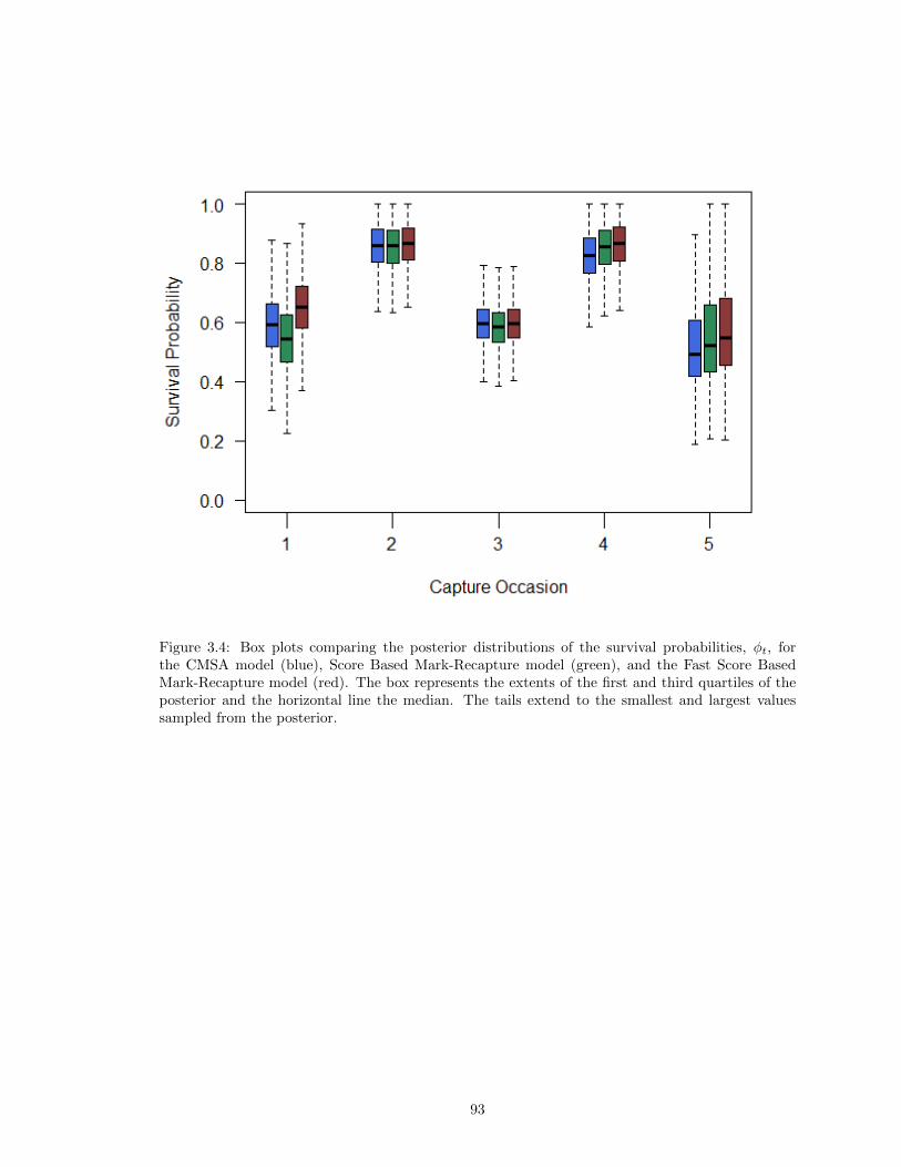
Figure 3.4: Box plots comparing the posterior distributions of the survival probabilities, φt, forthe CMSA model (blue), Score Based Mark-Recapture model (green), and the Fast Score BasedMark-Recapture model (red). The box represents the extents of the first and third quartiles of theposterior and the horizontal line the median. The tails extend to the smallest and largest valuessampled from the posterior.

93

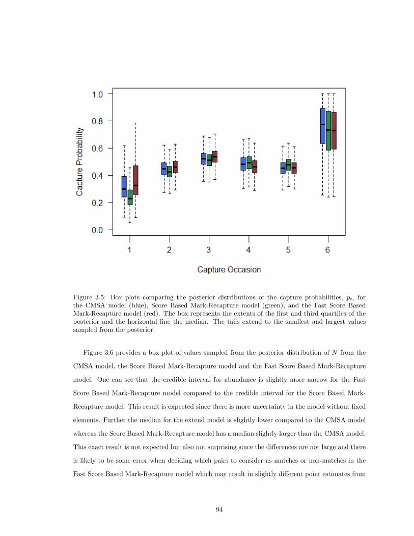
Figure 3.5: Box plots comparing the posterior distributions of the capture probabilities, pt, forthe CMSA model (blue), Score Based Mark-Recapture model (green), and the Fast Score BasedMark-Recapture model (red). The box represents the extents of the first and third quartiles of theposterior and the horizontal line the median. The tails extend to the smallest and largest valuessampled from the posterior.

Figure 3.6 provides a box plot of values sampled from the posterior distribution of N from the

CMSA model, the Score Based Mark-Recapture model and the Fast Score Based Mark-Recapture

model. One can see that the credible interval for abundance is slightly more narrow for the Fast

Score Based Mark-Recapture model compared to the credible interval for the Score Based Mark-

Recapture model. This result is expected since there is more uncertainty in the model without fixed

elements. Further the median for the extend model is slightly lower compared to the CMSA model

whereas the Score Based Mark-Recapture model has a median slightly larger than the CMSA model.

This exact result is not expected but also not surprising since the differences are not large and there

is likely to be some error when deciding which pairs to consider as matches or non-matches in the

Fast Score Based Mark-Recapture model which may result in slightly different point estimates from

94

the posterior.

Figure 3.6: Box plots comparing the posterior distributions of abundance, N , for the CMSA model,Score Based Mark-Recapture model, and the Fast Score Based Mark-Recapture model. The boxrepresents the extents of the first and third quartiles of the posterior and the vertical line the median.The tails extend to the smallest and largest values sampled from the posterior.

In order to compare the computational time required for the Score Based Mark-Recapture model

and the Fast Score Based Mark-Recapture model I ran a single chain from each sample for 1,000,000

iterations on the same machine started at the same seed value. The elapsed system time for the

Fast Score Based Mark-Recapture model was 27.1 hours and the elapsed time for the Score Based

Mark-Recapture model was 29.4 hours, indicating that the Fast Score Based Mark-Recapture model

did decrease the run time even though algorithm was only applied to the 18.5% of the data set.

3.4 Discussion

Previously in Chapter 2 I presented a general framework that addresses the issue of misidentification

in photographic identification. One downside to fitting the Score Based Mark-Recapture model with

MCMC was the computational time. In this chapter I proposed to a priori fix the relationship

95

between some pairs of photographs in order to reduced the sample space of C(X) conditional on Y

and reduce the computational time required to sample from the desired posterior distributions. It

was shown that by fixing elements of the the latent matrix of the true nature of each pair, C(X),

a priori either by application of auxiliary information or application of the proposed algorithm,

I may greatly reduce the sample space of C(X) conditional on Y. By determining some pairs

of photographs as matches or non-matches a priori I introduced dependencies in C(X), which

required the development of a new sampler. The whale shark example illustrates that even when

the algorithm to predetermine matches and non-matches can only be applied to a portion of the

data set computation time is reduced and similar results are obtained. Further the simulation study

illustrated that the Fast Score Based Mark-Recapture model provided similar posterior estimates

for the parameters of interest when compared to the Score Based Mark-Recapture model and the

CMSA model. Additionally the Fast Score Based Mark-Recapture model required less computation

time compared to the Score Based Mark-Recapture model and as the overlap between the mixture

distribution of the pairwise scores decreased the computation time of the Fast Score Based Mark-

Recapture model also decreased.

Although the methods presented in this chapter improve the speed of computation, catalogs

with large number of photographs will still require long computation times especially when there is

a large overlap between the density of the match and non-match scores. Further improvements are

still possible. Additionally the requirement of the estimation of the distribution of the scores for the

matches and non-matches is non-trivial and poor estimation may result in bias in the estimation of

the parameters of interest. In future work I would like to further improve the computation time by

developing further approximations of the posterior distributions of interest.

96

Chapter 4

Conclusion

4.1 Introduction

An extended hierarchical model that utilizes pairwise scores generated from pairs of photographs as

data was proposed in Chapter 2. This method is employed estimate different parameters of interest

from mark-recapture studies which utilize photographic identification as method of capture. The in-

corporation of pairwise scores as data is a new idea. This Score Based Mark-Recapture model is able

to easily incorporate different underlying mark-recapture models. Prior methods of modeling data

from mark-recapture studies, which utilize photographic identification as the method of capture,

required trained researchers to make a decision as to whether or not each pair of photographs depict

the same individual. The past models did not incorporate the uncertainty of the matching process in

the estimation of parameters. The process of identifying which photographs depict the same individ-

ual is a time consuming task even when computer algorithms are employed to assist researchers in

the decision making process. My method significantly reduces the need for the researcher to decide

which pairs of photographs depict the same individual by only requiring the true match status be

known for a training set of data. Once the distribution of scores originating from matching and

non-matching pairs is estimated from the training set no further action is needed by the researcher

in the matching process. Examining the results from the whale shark and simulated data, one can

see that parameter estimates from the Score Based Mark-Recapture model (with the CMSA model

as the underlying mark-recapture model) and the CMSA model fit with the true match/non-match

status of photographs produce similar results.

Sampling from the Score Based Mark-Recapture model proved to be computationally expensive.

In Chapter 3 an algorithm was presented to a priori determine some of the pairs to be matches

or non-matches based on the observed score generated between the two photographs. Through

simulation I was able to show that the required computational time decreased when comparing

the Score Based Mark-Recapture model to the Fast Score Based Mark-Recapture model with the

CMSA model as the underlying mark-recapture model. Additionally, as the separation between the

underlying distributions of the match and non-match scores separated the computational time also

improved. Even in cases such as the whale shark data, where only a small percentage of pairs are

able to be determined a priori, there are still improvements in the computation time.

In Chapters 2 and 3 I considered pairwise scores originating from the comparison of photographs

97

as data and proposed a Score Based Mark-Recapture model to account for the uncertainty in the

matching process. The presented methods are able to provide reasonable estimates of the parameters

by accounting for the inherent uncertainty of photographic identification, but there are several areas

for both extension and improvement which may be considered. In addition to improving the current

methods, there are many interesting avenues for future work that arise from the analysis of data

produced by citizen scientist.

4.2 Computational Improvement

In Chapter 3 I discussed the computational complexity of fitting the presented models. By restricting

the sample space I was able to approximate the posterior distribution and obtain results similar to

sampling from the full posterior. The restriction in sample space reduced the computational time but

the methods are still computationally expensive. Future improvements in computational efficiency

would make the methods easier to use and available to a wider audience.

Computational improvements may be possible in the estimation of abundance, N . Recall from

Chapter 2 that I consider a data set comprised of all possible pairwise scores from a set of pho-

tographs. I would like to infer from the scores the true nature of each pair, represented by C(X)

which is a Np × Np binary matrix, where Np represents the total number of photographs. Each

set of photographs creates an unique row in C(X) and the unique rows of C(X) are equal to the

number of animals that were observed in the study.

It may be possible to make inference about abundance based on the information contained in

C(X) without sampling W. It is possible to visualize the relationship by looking at the following

DAG.

98

N p

X

C

λ

Sobs

Figure 4.1: Directed Acyclic Graph (DAG) Representation of a Model for the Estimation of Abun-dance Not Incorporating an Underlying Mark-Recapture Model .

Looking at Figure 4.1 one can see that X is a function of how many animals are available

for capture (N), the probability of being photographed (p) and the rate of photography assuming

the animal is photographed once (λ). Alternatively it may be possible to redefine λ as the rate

of photography allowing for an animal not to be photographed and remove p from the model.

Considering X as a function of N , p and λ would allow for marginalizing over W, which would

greatly simplify the MCMC since integration of W would no longer be necessary. More work is

needed in developing the distributions for the model.

4.3 Extension to Other Underlying Mark-Recapture Models and Data Sets

Another area for future work is expansion of methods to incorporate more complex underlying

mark-recapture models. Collaborators would like to see the methods extended to incorporate an

Open Robust Design (ORD). In a robust the population is considered closed between some capture

occasions and open between others. (Link and Barker, 2009) The hierarchical model presented in

Chapter 2 allows for the ORD to easily be incorporated into the model. The sampler presented

in Chapter 2 will need to be adjusted to sample from the hierarchical model with the ORD as the

underlying mark-recapture model.

Currently I have only applied the methods to data originating from the pairwise comparison of

whale shark photographs. I also have access to pairwise comparison of photographs of humpback

whales. The pairwise scores for these photographs are generated under a different matching algorithm

and the distribution of the scores will need to be estimated. This set of photographs contains more

99

than 15,000 photographs, further emphasizing the need to improve the computational complexity of

the current methods.

4.4 Further Exploration of Citizen Scientist Data

As discussed in Chapter 1, citizen scientist are beginning to play an important role in ecological data

collection and analyzing this data poses some interesting questions that may lead to new avenues of

research.

4.4.1 Lack Experimental Design on Estimates of Abundance and Capture Probability

Photo identification from Ecotourism differs from traditional photo identification in that there is no

experimental design. I propose studying how this lack of experimental design affects the estimates

of survival and capture probability. To study the differences I will develop a simulation study.

• Step 1 (Define Region of interest): Consider an area divided evenly into different regions. Then

define animal abundance and movement across the regions.

• Step 2 (Experimental Design): Consider a camera in the center of each region, and simulate

the photos that would be taken.

• Step 3 (Ecotourism): Simulate data similar to how data is currently collected.

Currently whale shark sightings occur off the coast of Ningaloo Marine Park. In Ningaloo Park there

are 2 places where ecotourism routes start, one in the north and one in the south. Visual inspection

of the location of sightings suggest a relationship between locations of snorkeling tour office and

location of sightings. This is supported by Holmberg et al. (2008).

For the data simulated in step 3, I consider the area in step 1 and define a point away from the

area of interest to represent the snorkeling tour office. I then consider the distance from the office

to the center of each of the regions. Those regions closer to the office are more likely to capture a

photograph.

Once I simulate data and show the effect I will then incorporate the location of the office in the

model. This could be accomplished by weighting sightings based on proximity to the office.

100

4.4.2 Choice of Primary Occasions in Open Robust Design

An additional topic related to the whale shark data that I would like to examine is the treatment

of capture occasion as continuous vs. discrete. The application of the ORD is used in the study of

whale sharks with year as the primary and eight two-week time spans as the secondary Holmberg

et al. (2009). In general, when a model like this is considered a researcher collects data every two

weeks (or how ever the secondary time point is defined). Here the collection process is continuous

and the two week choice is arbitrary. I plan to look at the effect of the choice of secondary period

duration and see the effects on the parameter estimates for the ORD. The effect on the parameter

estimates would not be specifically for the model described in Chapter 2 but rather for the ORD.

Since the ORD may be considered as an underlying mark-recapture model for the model presented in

Chapter 2, any effect on the parameter estimates due to choice of secondary period duration would

also occur in the Score Based Mark-Recapture model. Schofield et al. (2017) recently examined how

to fit continuous-time models without forcing the data into distinct capture occasions. In particular

the paper focuses on models Mh and Mth.

101

Appendix A

Appendix

A.1 Cardinality of CY With and Without Restrictions

In Section 3.2 the effect of fixing elements of C(X) on the cardinality of CY was illustrated by

revisiting an example from Chapter 2. In order to illustrate the reduction in the cardinality of CY

which occurs when fixing elements of C(X) four different scenarios were considered:

1. Cardinality of CY with no restrictions

2. Cardinality of CY when non-matches are predetermined

3. Cardinality of CY when matches are predetermined

4. Cardinality of CY when non-matches and matches are predetermined.

Presented here are the detailed calculation for each cardinality. Recall the following realization of

Y from Section 3.2:

Y =

2 0 1 0 0

1 0 3 0 2

0 0 0 0 0

3 0 2 0 0

0 1 0 0 0

0 4 0 3 3

0 0 0 0 0

0 1 0 0 0

0 0 2 0 1

.

Additionally the photographs were taken on the following occasions:

• On occasion 1: 1, 8, 9, 15, 21 and 23

• On occasion 2: 3, 5, 11, 14, 18, and 22

• On occasion 3: 2, 4, 10, 12, 13, 16, 17 and 20

• On occasion 4: 6, 7 and 19

• On occasion 5: 24, 25, 26, 27, 28 and 29.

102

A.1.1 Cardinality of CY with No Restrictions

Previously Y·t denoted the total number of photographs taken on the tth occasion and the cardinality

of CY is given by:

#CY =

T∏t=1

[(Y·tY1,t

) N∏i=2

(Y·t −

∑i−1l=1 Yl,t

Yi,t

)].

For this example T = 5, Y· = (6, 6, 8, 3, 6), and

(Y·tY1,t

) N∏i=2

(Y·t −

∑i−1l=1 Yl,t

Yi,t

)=

(62

)(41

)(33

)t = 1(

61

)(54

)(11

)t = 2(

81

)(73

)(42

)(22

)t = 3(

33

)t = 4(

62

)(43

)(11

)t = 5

Therefore:

#CY = 60× 30× 1680× 1× 60 = 181, 440, 000.

A.1.2 Cardinality of CY when Non-Matches are Predetermined

Suppose, as in Section 3.2, that is was determined a priori that photos 1 and 23, 4 and 9, and 27

and 29 cannot be paired. Visualizing the restrictions:

• On occasion 1: 1, 8, 9, 15, 21 and 23

• On occasion 2: 3, 5, 11, 14, 18, and 22

• On occasion 3: 2, 4, 10, 12, 13, 16, 17 and 20

• On occasion 4: 6, 7 and 19

• On occasion 5: 24, 25, 26, 27, 28 and 29

where photographs with similar colors identify photographs which are known not to depict the same

individual. The cardinality of CY with these restrictions is calculated in two steps.

First, the cardinality accounting for restrictions caused by pairs of non-matching photographs

taken on the same occasion is calculated. In this case, pairs 1 and 23 and 4 and 9.

• On occasion 1:

– There are 60 possible combinations of the photographs.

103

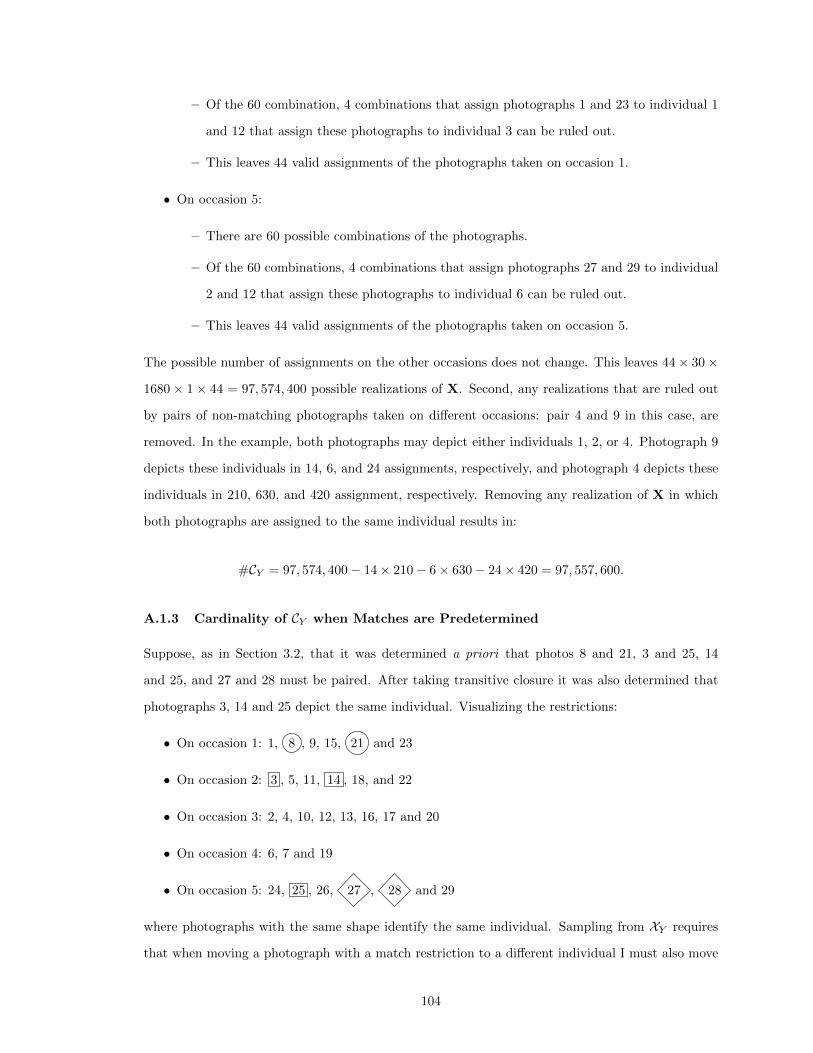
– Of the 60 combination, 4 combinations that assign photographs 1 and 23 to individual 1

and 12 that assign these photographs to individual 3 can be ruled out.

– This leaves 44 valid assignments of the photographs taken on occasion 1.

• On occasion 5:

– There are 60 possible combinations of the photographs.

– Of the 60 combinations, 4 combinations that assign photographs 27 and 29 to individual

2 and 12 that assign these photographs to individual 6 can be ruled out.

– This leaves 44 valid assignments of the photographs taken on occasion 5.

The possible number of assignments on the other occasions does not change. This leaves 44× 30×

1680 × 1 × 44 = 97, 574, 400 possible realizations of X. Second, any realizations that are ruled out

by pairs of non-matching photographs taken on different occasions: pair 4 and 9 in this case, are

removed. In the example, both photographs may depict either individuals 1, 2, or 4. Photograph 9

depicts these individuals in 14, 6, and 24 assignments, respectively, and photograph 4 depicts these

individuals in 210, 630, and 420 assignment, respectively. Removing any realization of X in which

both photographs are assigned to the same individual results in:

#CY = 97, 574, 400− 14× 210− 6× 630− 24× 420 = 97, 557, 600.

A.1.3 Cardinality of CY when Matches are Predetermined

Suppose, as in Section 3.2, that it was determined a priori that photos 8 and 21, 3 and 25, 14

and 25, and 27 and 28 must be paired. After taking transitive closure it was also determined that

photographs 3, 14 and 25 depict the same individual. Visualizing the restrictions:

• On occasion 1: 1, 8 , 9, 15, 21 and 23

• On occasion 2: 3 , 5, 11, 14 , 18, and 22

• On occasion 3: 2, 4, 10, 12, 13, 16, 17 and 20

• On occasion 4: 6, 7 and 19

• On occasion 5: 24, 25 , 26, 27 , 28 and 29

where photographs with the same shape identify the same individual. Sampling from XY requires

that when moving a photograph with a match restriction to a different individual I must also move

104

any photographs which are also known to depict the same individual. Photographs without match

restrictions, such as photograph 11, are free to move to any individual.

Calculating the cardinality with match restrictions is similar to the case with no restrictions.

Considering each occasion in sequence:

• On occasion 1

– Photographs 8 and 21 must depict the same individual, suggesting that the photographs

cannot depict individual 2.

– There are 4 combinations where photographs 8 and 21 depict individual 1 and 12 com-

binations where photographs 8 and 21 depict individual 4 resulting in 16 possible combi-

nations.

• On occasion 2

– Photographs 3, 14 and 25 must depict the same individual, suggesting that the pho-

tographs must depict individual 6 since individual 6 is the only individual depicted more

than once.

– There are 12 combinations where photographs 3 and 14 depict individual 6.

• On occasion 5

– Photographs 3, 14 and 25 must depict the same individual. Based on occasion 2 the

photographs must depict individual 6 since individual 6 is the only individual depicted

more than once on occasion 2.

– Photographs 27 and 28 also depict the same individual, suggesting that the photographs

cannot depict individual 9 since individual 9 was only photographed once.

– There are 3 combinations where photographs 27 and 28 depict individual 2 and photo-

graph 25 depicting individual 6 and 3 combinations where photographs 27, 28 and 9 depict

individual 6. There are 3+3=6 possible combinations which satisfy the match restriction

on occasion 5.

The possible number of assignments on the other occasions does not change. Accounting for the

match restrictions which occur within and across occasions results in:

#CY = 16× 12× 1680× 1× 6 = 1, 935, 360.

105

A.1.4 Cardinality of CY when Non-Matches and Matches are Predetermined

Suppose, as in Section 3.2, that it was determined a priori that photos 1 and 23, 4 and 9, and 27

and 29 cannot be paired. Additionally that photos 8 and 21, 3 and 25, 14 and 25, and 27 and 28

must be paired. After taking transitive closure it was determined that photographs 3, 14 and 25

depict the same individual. Visualizing the restrictions:

• On occasion 1: 1, 8 , 9, 15, 21 and 23

• On occasion 2: 3 , 5, 11, 14 , 18, and 22

• On occasion 3: 2, 4, 10, 12, 13, 16, 17 and 20

• On occasion 4: 6, 7 and 19

• On occasion 5: 24, 25 , 26, 27 , 28 and 29/29

where photographs with the same color denote photographs which are known not to identify the same

individual and photographs with the same shape identify photographs which are known to depict

the same individual. Sampling from XY requires that when moving a photograph any photographs

which depict the same individual must also be moved while not violating a non-match restriction.

In order to calculate the cardinality with non-match restrictions and match restrictions I consider

the combinations which satisfy the match restrictions and further consider the non-match restrictions

within and across capture occasions.

• On occasion 1

– Photographs 8 and 21 must depict the same individual, suggesting that the photographs

cannot depict individual 2. Additionally photographs 1 and 23 cannot depict the same

individual.

∗ If photographs 8 and 21 depict individual 1 then photographs 1 and 23 must sepa-

rately depict either individual 2 or 4, suggesting there are 2 possible combinations.

∗ If photographs 8 and 21 depict individual 4 there are 10 possible combinations which

do not have photographs 1 and 23 depicting the same individual.

– Resulting in 2+10=12 possible combinations which satisfy the non-match and match

restriction on occasion 1.

• On occasion 2

106

– The restriction exist that photographs 3, 14 and 25 must depict the same individual,

suggesting that the photographs must depict individual 6 since individual 6 is the only

individual depicted more than once.

– There are 12 combinations where photographs 3 and 14 depict individual 6.

• On occasion 5

– The restriction exist that photographs 3, 14 and 25 must depict the same individual.

Based on occasion 2 it is known that the photographs must depict individual 6 since

individual 6 is the only individual depicted more than once on occasion 2.

– Additionally the restriction that photographs 27 and 28 also depict the same individual,

suggest that the photographs cannot depict individual 9 since individual 9 was only

photographed once.

– There are 3 combinations where photographs 27 and 28 depict individual 2 and photo-

graph 25 depicting individual 6. There are 3 combinations where photographs 27, 28 and

9 depict individual 6.

– There are 3+3=6 possible combinations which satisfy the match restriction on occasion

5.

– There exist the non-match restriction that photographs 27 and 29 cannot depict the same

individual. Considering the 6 possible combinations which satisfy the match restrictions

above, none of the combinations suggest that photographs 27 and 29 depict the same

individual.

– There are 6 combinations which satisfy the non-match and match restrictions.

The possible number of assignments on the other occasions does not change. Accounting for the

match and non-match restrictions which occur within an occasion results in:

#CY = 12× 12× 1680× 1× 6 = 1, 415, 520.

Second, realizations ruled out by pairs of non-matching photographs taken on different occasions:

pair 4 and 9 in this case, are removed. In the example, both photographs may depict either individ-

uals 1, 2, or 4. Photograph 9 depicts these individuals in 6, 3, and 3 assignments, respectively, and

photograph 4 depicts these individuals in 210, 630, and 420 assignment, respectively. Removing any

107

realization of X in which both photographs are assigned to the same individual resulting in:

#CY = 1, 415, 520− 6× 210− 3× 630− 3× 420 = 1, 447, 110.

108

Bibliography

Steven C Amstrup, Trent L McDonald, and Bryan FJ Manly. Handbook of capture-recapture analysis.Princeton University Press, 2010.

Carlos JR Anderson, Niels Da Vitoria Lobo, James D Roth, and Jane M Waterman. Computer-aidedphoto-identification system with an application to polar bears based on whisker spot patterns.Journal of Mammalogy, 91(6):1350–1359, 2010.

AN Arnason and KH Mills. Bias and loss of precision due to tag loss in jolly–seber estimates formark–recapture experiments. Canadian Journal of Fisheries and Aquatic Sciences, 38(9):1077–1095, 1981.

Z Arzoumanian, J Holmberg, and B Norman. An astronomical pattern-matching algorithm forcomputer-aided identification of whale sharks Rhincodon typus. Journal of Applied Ecology, 42(6):999–1011, 2005.

Carley S Bansemer and Mike B Bennett. Multi-year validation of photographic identification of greynurse sharks, carcharias taurus, and applications for non-invasive conservation research. Marineand Freshwater Research, 59(4):322–331, 2008.

BWPM Beekmans, Hal Whitehead, Ruben Huele, Lisa Steiner, and Adri G Steenbeek. Compar-ison of two computer-assisted photo-identification methods applied to sperm whales (Physetermacrocephalus). Aquatic Mammals, 31(2):243, 2005.

John Adrian Bondy and Uppaluri Siva Ramachandra Murty. Graph theory, volume 244 of. Graduatetexts in Mathematics, 2008.

Simon Bonner and Jason Holmberg. Mark-recapture with multiple, non-invasive marks. Biometrics,69(3):766–775, 2013.

Simon J Bonner, Matthew R Schofield, Patrik Noren, Steven J Price, et al. Extending the latentmultinomial model with complex error processes and dynamic markov bases. The Annals ofApplied Statistics, 10(1):246–263, 2016.

Gary R Bortolotti. Effect of nest-box size on nest-site preference and reproduction in americankestrels. Journal of Raptor Research, 28(3):127–133, 1994.

Stephen P Brooks and Andrew Gelman. General methods for monitoring convergence of iterativesimulations. Journal of computational and graphical statistics, 7(4):434–455, 1998.

J Calambokidis, GH Steiger, JC Cubbage, KC Balcomb, C Ewald, S Kruse, R Wells, and R Sears.Sightings and movements of blue whales off central california 1986-88 from photo-identification ofindividuals. Report of the International Whaling Commission (special issue 12), pages 343–348,1990.

George Casella and Edward I George. Explaining the Gibbs sampler. The American Statistician,46(3):167–174, 1992.

Rolando Basim Chuaqui. Axiomatic set theory, volume 51. Newnes, 2011.

Jeffrey P Cohn. Citizen science: Can volunteers do real research? BioScience, 58(3):192–197, 2008.

RM Cormack. Estimates of survival from the sighting of marked animals. Biometrika, 51(3/4):429–438, 1964.

Laura Cowen and Carl J Schwarz. The jolly–seber model with tag loss. Biometrics, 62(3):699–705,2006.

109

Jonathan P Crall, Charles V Stewart, Tanya Y Berger-Wolf, Daniel I Rubenstein, and Siva RSundaresan. Hotspotter-patterned species instance recognition. pages 230–237, 2013.

SF Crosbie and BFJ Manly. Parsimonious modelling of capture-mark-recapture studies. Biometrics,pages 385–398, 1985.

Tricia L Cutler and Don E Swann. Using remote photography in wildlife ecology: a review. WildlifeSociety Bulletin, pages 571–581, 1999.

JN Darroch. The multiple-recapture census. Biometrika, 46(3-4):336–351, 1959.

Ivan P Fellegi and Alan B Sunter. A theory for record linkage. Journal of the American StatisticalAssociation, 64(328):1183–1210, 1969.

RM Fewster, BC Stevenson, David L Borchers, et al. Trace-contrast models for capture–recapturewithout capture histories. Statistical Science, 31(2):245–258, 2016.

Andrew Gelman and Donald B Rubin. Inference from iterative simulation using multiple sequences.Statistical science, pages 457–472, 1992.

Andrew Gelman, John B Carlin, Hal S Stern, and Donald B Rubin. Bayesian data analysis, volume 2.Chapman & Hall/CRC Boca Raton, FL, USA, 2014.

Stuart Geman and Donald Geman. Stochastic relaxation, gibbs distributions, and the bayesianrestoration of images. IEEE Transactions on pattern analysis and machine intelligence, (6):721–741, 1984.

Wally R Gilks, NG Best, and KKC Tan. Adaptive rejection Metropolis sampling within Gibbssampling. Applied Statistics, pages 455–472, 1995.

Peter J Green. Reversible jump Markov chain Monte Carlo computation and Bayesian model deter-mination. Biometrika, 82(4):711–732, 1995.

Chrysoula Gubili, Ryan Johnson, Enrico Gennari, W Hermann Oosthuizen, Deon Kotze, MikeMeyer, David W Sims, Catherine S Jones, and Leslie Robert Noble. Concordance of geneticand fin photo identification in the great white shark, Carcharodon carcharias, off Mossel Bay,South Africa. Marine Biology, 156(10):2199–2207, 2009.

C Guinet. Killer whales around possession-island, crozet archipelago-photo-identification 1964-1986.MAMMALIA, 52(2):285–289, 1988.

Kelly K Hastings, Lex A Hiby, and Robert J Small. Evaluation of a computer-assisted photograph-matching system to monitor naturally marked harbor seals at tugidak island, alaska. Journal ofMammalogy, 89(5):1201–1211, 2008.

W Keith Hastings. Monte carlo sampling methods using markov chains and their applications.Biometrika, 57(1):97–109, 1970.

Lex Hiby, Phil Lovell, Narendra Patil, N Samba Kumar, Arjun M Gopalaswamy, and K UllasKaranth. A tiger cannot change its stripes: using a three-dimensional model to match images ofliving tigers and tiger skins. Biology Letters, pages rsbl–2009, 2009.

GR Hillman, B Wursig, GA Gailey, N Kehtarnavaz, A Drobyshevsky, BN Araabi, HD Tagare, andDW Weller. Computer-assisted photo-identification of individual marine vertebrates: a multi-species system. Aquatic Mammals, 29(1):117–123, 2003.

Jason Holmberg. Wildbook for whale sharks, May 2003. URL https://www.whaleshark.org/.

Jason Holmberg, Bradley Norman, and Zaven Arzoumanian. Robust, comparable population metricsthrough collaborative photo-monitoring of whale sharks Rhincodon typus. Ecological Applications,18(1):222–233, 2008.

110

Jason Holmberg, Bradley Norman, and Zaven Arzoumanian. Estimating population size, structure,and residency time for whale sharks Rhincodon typus through collaborative photo-identification.Endangered Species Research, 7:39–53, 2009.

Herve Jegou, Matthijs Douze, and Cordelia Schmid. Improving bag-of-features for large scale imagesearch. International Journal of Computer Vision, 87(3):316–336, 2010.

George M Jolly. Explicit estimates from capture-recapture data with both death and immigration-stochastic model. Biometrika, 52(1/2):225–247, 1965.

K Ullas Karanth and James D Nichols. Estimation of tiger densities in india using photographiccaptures and recaptures. Ecology, 79(8):2852–2862, 1998.

Michael B Keck. Test for detrimental effects of pit tags in neonatal snakes. Copeia, 1994(1):226–228,1994.

William L Kendall, Catherine A Langtimm, Cathy A Beck, and Michael C Runge. Capture-recaptureanalysis for estimating manatee reproductive rates. Marine Mammal Science, 20(3):424–437, 2004.

Catherine A Langtimm, Cathy A Beck, Holly H Edwards, Kristin J Fick-Child, Bruce B Ackerman,Sheri L Barton, and Wayne C Hartley. Survival estimates for florida manatees from the photo-identification of individuals. Marine Mammal Science, 20(3):438–463, 2004.

Jean-Dominique Lebreton, Kenneth P Burnham, Jean Clobert, and David R Anderson. Modelingsurvival and testing biological hypotheses using marked animals: a unified approach with casestudies. Ecological monographs, 62(1):67–118, 1992.

William A Link and Richard J Barker. Modeling association among demographic parameters inanalysis of open population capture–recapture data. Biometrics, 61(1):46–54, 2005.

William A Link and Richard J Barker. Bayesian Inference: with Ecological Applications. AcademicPress, 2009.

William A Link, Jun Yoshizaki, Larissa L Bailey, and Kenneth H Pollock. Uncovering a latentmultinomial: analysis of mark–recapture data with misidentification. Biometrics, 66(1):178–185,2010.

Paul M Lukacs. Statistical aspects of using genetic markers for individual identification in capture-recapture studies. PhD thesis, Colorado State University Fort Collins, USA, 2005.

Paul M Lukacs and Kenneth P Burnham. Research notes: Estimating population size from dna-basedclosed capture–recapture data incorporating genotyping error. Journal of Wildlife Management,69(1):396–403, 2005.

David J. Lunn, Andrew Thomas, Nicky Best, and David Spiegelhalter. Winbugs &ndash; a bayesianmodelling framework: Concepts, structure, and extensibility. Statistics and Computing, 10(4):325–337, October 2000. ISSN 0960-3174.

Michael A McCarthy and Kirsten M Parris. Clarifying the effect of toe clipping on frogs withbayesian statistics. Journal of Applied Ecology, 41(4):780–786, 2004.

Brett T McClintock, Paul B Conn, Robert S Alonso, and Kevin R Crooks. Integrated modeling ofbilateral photo-identification data in mark–recapture analyses. Ecology, 94(7):1464–1471, 2013.

Trent L McDonald, Steven C Amstrup, and Bryan FJ Manly. Tag loss can bias jolly-seber capture-recapture estimates. Wildlife Society Bulletin, pages 814–822, 2003.

Nicholas Metropolis, Arianna W Rosenbluth, Marshall N Rosenbluth, Augusta H Teller, and EdwardTeller. Equation of state calculations by fast computing machines. The journal of chemical physics,21(6):1087–1092, 1953.

111

Alvaro E. Monge. Matching algorithms within a duplicate detection system. IEEE Data Eng. Bull.,23(4):14–20, 2000.

Thomas A Morrison, Jun Yoshizaki, James D Nichols, and Douglas T Bolger. Estimating survival inphotographic capture–recapture studies: overcoming misidentification error. Methods in Ecologyand Evolution, 2(5):454–463, 2011.

Garth Mowat and Curtis Strobeck. Estimating population size of grizzly bears using hair capture,dna profiling, and mark-recapture analysis. The Journal of wildlife management, pages 183–193,2000.

David L Otis, Kenneth P Burnham, Gary C White, and David R Anderson. Statistical inferencefrom capture data on closed animal populations. Wildlife monographs, pages 3–135, 1978.

Mark A Paulissen and Harry A Meyer. The effect of toe-clipping on the gecko hemidactylus turcicus.Journal of Herpetology, 34(2):282–285, 2000.

Carl Georg Johannes Petersen. The yearly immigration of young plaice into the limfjord from thegerman sea. Report of the Danish Biological Station, 6:1–48, 1896.

Kenneth H Pollock, James D Nichols, Cavell Brownie, and James E Hines. Statistical inference forcapture-recapture experiments. Wildlife monographs, pages 3–97, 1990.

Roger Pradel, James E Hines, Jean-Dominique Lebreton, and James D Nichols. Capture-recapturesurvival models taking account of transients. Biometrics, pages 60–72, 1997.

R Core Team. R: A Language and Environment for Statistical Computing. R Foundation forStatistical Computing, Vienna, Austria. URL https://www.R-project.org.

DS Robson and HA Regier. Estimates of tag loss from recoveries of fish tagged and permanentlymarked. Transactions of the American Fisheries Society, 95(1):56–59, 1966.

Fabrizio Ruggeri, Ron S Kenett, and Frederick W Faltin. Encyclopedia of statistics in quality andreliability, 2007.

Mauricio Sadinle and Stephen E Fienberg. A generalized fellegi–sunter framework for multiplerecord linkage with application to homicide record systems. Journal of the American StatisticalAssociation, 108(502):385–397, 2013.

Pedro Bernardo Sarmento, Joana P Cruz, Catarina I Eira, and Carlos Fonseca. Habitat selectionand abundance of common genets genetta genetta using camera capture-mark-recapture data.European journal of wildlife research, 56(1):59–66, 2010.

Matthew R Schofield and Richard J Barker. A unified capture-recapture framework. Journal ofagricultural, biological, and environmental statistics, 13(4):458–477, 2008.

Matthew R Schofield and Simon J Bonner. Connecting the latent multinomial. Biometrics, 71(4):1070–1080, 2015.

Matthew R Schofield, Richard J Barker, and Nicholas Gelling. Continuous-time capture–recapturein closed populations. Biometrics, 2017.

Carl James Schwarz and A Neil Arnason. A general methodology for the analysis of capture-recaptureexperiments in open populations. Biometrics, pages 860–873, 1996.

GAF Seber. Estimating time-specific survival and reporting rates for adult birds from band returns.Biometrika, 57(2):313–318, 1970.

G.A.F. Seber. The Estimation of Animal Abundance and Related Parameters. Blackburn Press,2002. ISBN 9781930665552.

112

George Seber. A note on the multiple-recapture census. Biometrika, 52(1/2):249–259, 1965.

George Arthur Frederick Seber and R Felton. Tag loss and the petersen mark-recapture experiment.Biometrika, pages 211–219, 1981.

Richard F. Shepard. Berenice abbott: Still feisty and eager at 91. The New York Times, 1989.

Jonathan Silvertown. A new dawn for citizen science. Trends in ecology & evolution, 24(9):467–471,2009.

Rebecca C Steorts, Rob Hall, and Stephen E Fienberg. Smered: A Bayesian approach to graphicalrecord linkage and de-duplication. arXiv preprint arXiv:1403.0211, 2014.

Peter T Stevick, Per J Palsbøll, Tim D Smith, Mark V Bravington, and Philip S Hammond. Errorsin identification using natural markings: rates, sources, and effects on capture recapture estimatesof abundance. Canadian Journal of Fisheries and Aquatic Sciences, 58(9):1861–1870, 2001.

Andrea Tancredi, Brunero Liseo, et al. A hierarchical bayesian approach to record linkage andpopulation size problems. The Annals of Applied Statistics, 5(2B):1553–1585, 2011.

Andrea Tancredi, Marie Auger-Methe, Marianne Marcoux, and Brunero Liseo. Accounting formatching uncertainty in two stage capture–recapture experiments using photographic measure-ments of natural marks. Environmental and ecological statistics, 20(4):647–665, 2013.

Luke Tierney. Markov chains for exploring posterior distributions. the Annals of Statistics, pages1701–1728, 1994.

Mogens Trolle and Marc Kery. Estimation of ocelot density in the pantanal using capture–recaptureanalysis of camera-trapping data. Journal of mammalogy, 84(2):607–614, 2003.

AM Van Tienhoven, JE Den Hartog, RA Reijns, and VM Peddemors. A computer-aided program forpattern-matching of natural marks on the spotted Raggedtooth shark Carcharias taurus. Journalof Applied Ecology, 44(2):273–280, 2007.

C Vincent, L Meynier, and V Ridoux. Photo-identification in grey seals: legibility and stability ofnatural markings. Mammalia, 65(3):363–372, 2001.

JERRY A Wetherall. Analysis of double-tagging experiments. Fish. Bull, 80(4):687–701, 1982.

Deborah J Wilson, Murray G Efford, Samantha J Brown, John F Williamson, and Gary J McElrea.Estimating density of ship rats in new zealand forests by capture-mark-recapture trapping. NewZealand Journal of Ecology, pages 47–59, 2007.

Janine A Wright, Richard J Barker, Matthew R Schofield, Alain C Frantz, Andrea E Byrom, andDianne M Gleeson. Incorporating genotype uncertainty into mark–recapture-type models forestimating abundance using dna samples. Biometrics, 65(3):833–840, 2009.

Jun Yoshizaki. Use of natural tags in closed population capture-recapture studies: modeling misiden-tification. 2007.

Jun Yoshizaki, Kenneth H Pollock, Cavell Brownie, and Raymond A Webster. Modeling misiden-tification errors in capture-recapture studies using photographic identification of evolving marks.Ecology, 90(1):3–9, 2009.

113

Vita

• Amanda R. Ellis, Lexington, Kentucky

• Education

– M.S. in Statistics: University of Kentucky, 2013.

– B.S. in Mathematics: University of Kentucky, 2009.

• Professional Experience

– Graduate Teaching Assistant, Department of Statistics, University of Kentucky, 2011-2017.

• Scholastic Honors

– Spring Chapter Meeting KYASA: Student Research Symposium Best Talk Award, Lex-ington KY, 2016.

– Provost Outstanding Teaching, University of Kentucky (University Award), 2015.

– R.L. Anderson Award for Outstanding Teaching, UK Department of Statistics, 2012.

– College of Arts and Sciences Certificate for Outstanding Teaching, University of Kentucky,2012.

– Boyd Hershberger Travel Award, provided by National Science Foundation to attendSRCOS, 2012.

• Publications

– Nardone, R., Heller, Y., Thomschewski, A., Bathke, A. C., Ellis, A. R., Golaszewski,S. M., Trinka, E. (2015). Assessment of corticospinal excitability after traumatic spinalcord injury using MEP recruitment curves: a preliminary TMS study. Spinal cord.

– Ellis, A. R., Burchett, W., Bathke, A. C.,Harrar, S. (2017). Nonparametric Inference forMultivariate Data: The R Package npmv. Journal of Statistical Software.

– Ellis, A. R., Rayens, W. (2015). Creating a Student-Centered Learning EnvironmentOnline. Journal of Statistical Education. Submitted.

114