Embed Size (px)
Citation preview

Accounting for Macro-Finance Trends:
Market Power, Intangibles, and Risk Premia�
Emmanuel Farhiy and François Gourioz
October 2018
Abstract
Real risk-free interest rates have trended down over the past 30 years. Puzzlingly in light of this
decline, (1) the return on private capital has remained stable or even increased, creating an increasing
wedge with safe interest rates; (2) stock market valuation ratios have increased only moderately;
(3) investment has been lackluster. We use a simple extension of the neoclassical growth model
to diagnose the nexus of forces that jointly accounts for these developments. We �nd that rising
market power, rising unmeasured intangibles, and rising risk premia, play a crucial role, over and
above the traditional culprits of increasing savings supply and technological growth slowdown.
JEL codes: E34, G12.
Keywords: equity premium, risk-free rate, investment, pro�tability, valuation ratios, labor share,
competition, markups, safe assets.
1 Introduction
Over the past thirty years, most developed economies have experienced large declines in risk-free interest
rates and increases in asset prices such as housing or stock prices, with occasional sudden crashes. At
the same time, and apart from a short period in the 1990s, economic growth, in particular productivity
growth, has been rather disappointing, and investment has been lackluster. Earnings growth of cor-
porations has been strong however, leading in most countries to an increase in the capital share and
to stable or slightly rising pro�tability ratios. Making sense of these trends is a major endeavor for
macroeconomists and for �nancial economists.�The views expressed here are those of the authors and do not necessarily represent those of the Federal Reserve Bank
of Chicago or the Federal Reserve System. We thank participants in presentations at the Brookings conference, at the ECB
2018 research conference, SED 2017, SAET 2017, CEPR Asset-prices and the macroeconomy 2018, NBER Capital Markets
and the Economy 2018, the 2018 San Francisco Fed �nance conference, at the Chicago and Minneapolis Fed, and in the
Hoover institute conference in honor of John Cochrane, for their comments. We especially thank Stefania d�Amico, Marco
Bassetto, Bob Barsky, Gadi Barlevy, Je¤ Campbell, John Cochrane, Lars Hansen, Monika Piazzesi, Martin Schneider,
Sam Schulhofer-Wohl, Venky Venkateswaran, François Velde, our discussants Riccardo Colacito, Mark Gertler, Martin
Lettau, Dimitris Papanikolaou, Matthew Rognlie, and Jaume Ventura, and the editors Jan Eberly and James Stock for
their comments.yHarvard University and NBER; Email: [email protected] Reserve Bank of Chicago; Email: [email protected].
1
Given the complexity of these phenomena, it is tempting to study them in isolation. For instance, a
large literature has developed that tries to understand the decline in risk-free interest rates. But studying
these trends independently may miss confounding factors or implausible implications. For instance, an
aging population leads to higher savings supply which might well explain the decline in interest rates.
However, higher savings supply should also reduce pro�tability, and increase both investment and stock
prices. Hence, a potential driver that is compelling judged on its ability to explain a single trend, may
be implausible overall, because it makes it harder to account for the other trends.
Another way to highlight these tensions is to note that the stable pro�tability of private capital and
declining risk-free rate lead to a rising wedge, or spread, between these two rates of return. What gives
rise to this spread? A narrative that has been recently attracted signi�cant interest is the possibility of
rising market power. On the other hand, rising risk premia could also account for the wedge. The only
way to disentangle these potential causes is to consider additional implications - for instance, everything
else equal, rising market power should imply a lower labor share, and rising risk premia should be
re�ected in lower prices of risky assets such as stocks.
These simple observations motivate our approach. We believe that a successful structural analysis
of the past thirty years should account for these trends jointly. A novel feature of our analysis is that
we aim to account both for macro trends and �nance trends. The �rst step of our paper is to document
a set of broad macro-�nance trends which we believe are of particular interest. We focus on six broad
indicators, that involve the evolution of economic growth, risk-free interest rates, pro�tability, the capital
share, investment, and valuation ratios (such as the price-dividend or price-earnings ratio).
The second step in our paper is to develop an accounting framework to disentangle several potential
drivers of these trends. We focus on �ve broad narratives that have been put forward to explain some
or all of these trends. The �rst narrative is that the economy experienced a sustained growth decline,
owing to lower population growth, investment-speci�c technical progress, or productivity growth. The
second narrative is that savings supply has increased, perhaps owing to population aging (or to the
demand of emerging markets for store of values). A third narrative involves rising market power of
corporations. A fourth narrative focuses on technological change, coming from the introduction of
information technology, which may have favored capital or skilled labor over unskilled labor, or the
rise of hard-to-measure intangible forms of capital. A �fth narrative, which we will emphasize, involves
changes in perceived macroeconomic risk or of tolerance towards it.
Our approach is simple enough to allow for a relatively clear identi�cation of the impact of these
drivers on the facts that we target. Here our contribution is to propose a simple macroeconomic frame-
work - a modest extension of the neoclassical growth model - that allows to account for the �big ratios�
familiar to macroeconomists as well as for the ��nancial ratios� of �nancial economists. The familiar
di¢ culty here is the disconnect between macro and �nance, e.g. the equity premium puzzle: it is di¢ cult
to use macro models to �t asset price data. Our model does this in a way that allows for interesting
feedbacks between macroeconomic and �nancial variables. For example, the investment-output ratio is
a¤ected by market power and macroeconomic risk as well as savings supply and technological parame-
ters. At the same time, our framework preserves the standard intuition and results of macroeconomists
2
and �nancial economists, and hence serves a useful pedagogical purpose.
In our baseline estimation, we abstract from intangibles. Our main empirical result here is that the
rising spread between the return on capital is the risk-free rate is driven mostly by a con�uence of two
factors: rising market power and rising macroeconomic risk. This rising macroeconomic risk in turns
implies that the equity premium, which previous researchers have argued fell in the 1980s and 1990s,
may have risen since around 2000. Moreover, we show how previous researchers, who have used models
without risk, have attributed too big a role to rising market power. We also �nd little role for technical
change. Our estimates o¤er a better understanding of the drivers of investment, pro�tability, and
valuation ratios. Finally, stepping outside of the model, we provide further independent corroborative
evidence of the increase in the equity premium using simple reduced-form methods.
When we incorporate intangibles, we see that a signi�cant increase in their unmeasured component
can help explain the rising wedge between the measured marginal product of capital and the risk-free
rate. Interestingly, we �nd that intangible capital reduces the estimated role of market power in our
accounting framework, while preserving the role of risk.
The rest of the paper is organized as follows. The remainder of the introduction discusses the related
literature. Section 2 documents the main trends of interest. Section 3 presents our model, which is a
modest generalization of the neoclassical growth model. Section 4 explains our empirical methodology
and identi�cation. Section 5 presents the main empirical results. Section 6 discusses some extensions
and robustness. Finally, section 7 discusses some outside evidence on the rise in the equity premium,
markups, and intangibles. Section 8 concludes.
1.1 Literature review
Our paper, given its broad scope, makes contact with many other studies that have separately tried to
understand one of the key trends we document. We discuss in more detail the relation of our results to
the recent literature on market power, intangibles and risk premia in section 7.
First, there is a large literature that studies the decline of interest rates on government bonds.
Hamilton et al. (2015) provide a long-run perspective, and discuss the connection between growth and
the interest rates. Rachel and Smith (2017) is an exhaustive analysis of the role of many factors that
a¤ect interest rates. Carvalho et al. (2016) and Gagnon et al. (2016) study the role of demographics
in detail. Del Negro et al. (2017) emphasize the role of the safety and liquidity premia. Bernanke
(2005) and Caballero et al. (2005) emphasize the role of safe asset supply and demand. Our analysis
will incorporate all these factors, though in a simple way.
Second, a large literature documents and tries to understand the decline of the labor share in de-
veloped economies. Elsby et al. (2013) document the facts and discuss various explanations using US
data, while Karabarbounis and Neiman (2013) study international data and argue that the decline is
driven by investment-biased technical change. Rognlie (2015) studies the role of housing. A number of
other papers discuss the impact of technical change for a broader set of facts; see for instance Acemoglu
and Restreppo (2017), Autor et al. (2017), Kehrig and Vincent (2018), Van Reenen (2017).
Perhaps the most closely related papers are Caballero et al. (2017), Marx, Mojon and Velde (2017)
3
and the contemporaneous work by Eggertsson, Robins and Wold (2018). Marx, Mojon and Velde (2017)
also �nd, using a di¤erent methodology, that an increase in risk may explain the observed pattern for
the risk-free rate. They do not explicitly target the evolution of other variables such as investment or
the price-dividend ratio. On the other hand, Eggertsson, Robins and Wold (2018) target some of the
same big ratios that we study, but there are di¤erences in terms of methodology and in terms of results.
Methodologically, our approach uses a more standard and simple model, which allows a closed-form
solution and clear identi�cation. Substantively, we �nd a more important role for macroeconomic risk
whereas they contend that rising market power is the main driving force.
2 Some macro-�nance trends
This section presents simple evidence on the trends a¤ecting some key macro-�nance moments. We focus
on six groups of indicators: interest rates on safe and liquid assets such as government bonds, measures
of the rate of return on private capital, valuation ratios (i.e., price-dividend or price-earnings ratio for
publicly listed companies), private investment in new capital, the labor share, and growth trends. We
�rst present simple graphical depictions, then add some statistical measures.
Our focus is on the United States, but we believe that these facts hold in other developed economies
and hence likely re�ect worldwide trends. Like many macroeconomic studies, we will mostly consider the
post-1984 period, which is associated with low and stable in�ation together with relative macroeconomic
stability (the �Great Moderation�). We present the changes in the simplest possible way by breaking
our sample equally in the middle, i.e. at the millennium. However, we will also discuss brie�y the longer
trends and present continuous indicators using moving averages.
One important decision is whether to study the entire private sector, or to exclude housing and focus
for instance on non�nancial corporations. On one hand, the savings of households include all assets,
in particular housing; on the other hand, the housing sector may need to be modeled di¤erently, or we
might want to explicitly recognize the heterogeneity of capital goods. We will in this section present
indicators that cover both, but our estimation targets will cover the entire private sector. For the most
part, the trends that we document are apparent both for non�nancial corporations and in the aggregate.
2.1 Graphical evidence
We summarize the evolution of the six groups of indicators as six facts.
Fact #1: Real risk-free interest rates have fallen substantially
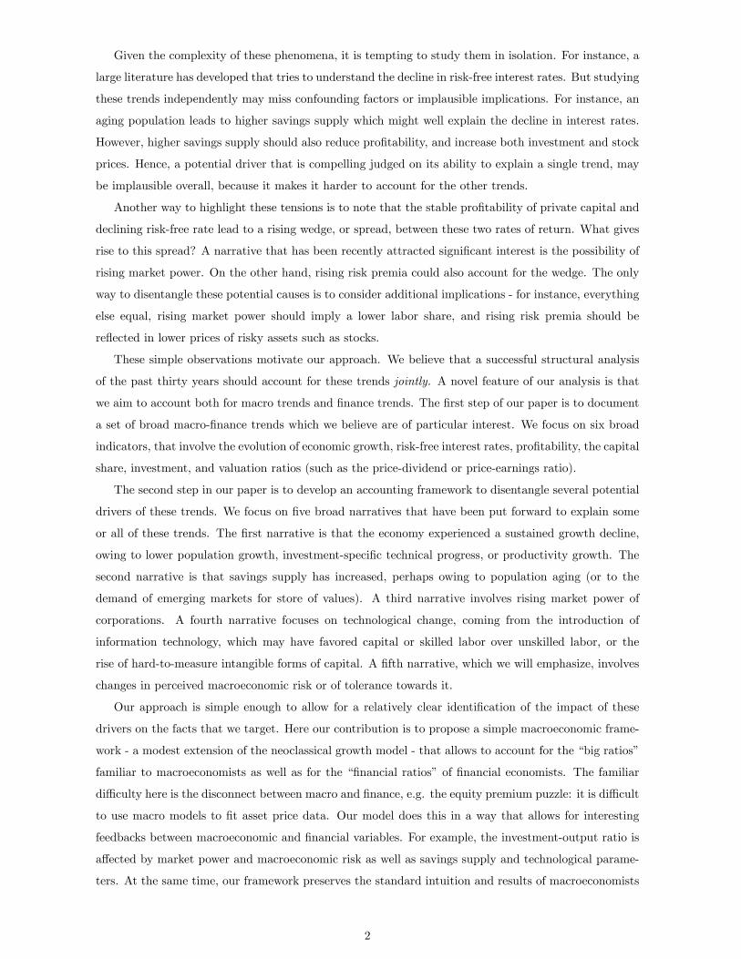
The top panels of �gure 1 present proxies for the one-year and ten-year real interest rates by sub-
stracting in�ation expectations from nominal Treasury yields.1 As many authors have noted before,
there has been a strong downward trend in these measures since 1984. The short-rate exhibits some
1We use median consumer price in�ation expectations from the Philadelphia Fed survey of professional forecasters
(SPF). Very similar results for the trend are obtained if one uses the mean expectation rather than the median; or the
Michigan survey of consumers rather than the SPF. For the one-year rate, one can also replace expectations with ex-post
in�ation or lagged in�ation. For the ten-year rate, one can also use the TIPS yield where available (i.e. post 1997).
4
clear cyclical �uctuations, while the long rate has a smoother decline. Table 1 shows that the average
one-year rate falls from around 2.8% in the �rst half of our sample (1984�2000) to -0.3% in the second
half of our sample (2001-2016). The long-term rate similarly falls from 3.9% in the �rst half to 1.1% in
the second half.
Fact #2: The pro�tability of private capital has remained stable or increased slightly
In contrast, there is little evidence that the return on private capital has fallen; if anything, it
appears to have increased slightly. Gomme, Ravikumar and Rupert (2011; thereafter GRR) construct
from national income (NIPA) data a measure of aggregate net return on physical capital, roughly
pro�ts over capital. The bottom left panel of �gure 1 depicts their series. The rising spread between
their measure, which can be thought as a proxy for the marginal product of capital, and the interest
rate on US Treasuries, is an important trend to be explained for macro- and �nancial economists.
GRR construct their series using detailed data from NIPA and other sources, but one can construct
a simple approximation using the ratio of operating surplus to capital for the non�nancial corporate
sector; Table 1 show that this ratio is also fairly constant. In our estimation exercise, we will focus
on gross pro�tability, and, to ensure consistency between our measures, will construct it simply as the
ratio of the pro�t-output ratio that we will use (i.e., one minus the labor share) to the capital-output
ratio. This measure is depicted in the bottom right panel of �gure 1; the overall level is higher, in part
because it is gross rather than net, but the trend is similar to the GRR measure.
Fact #3: Valuation ratios are stable or have increased moderately
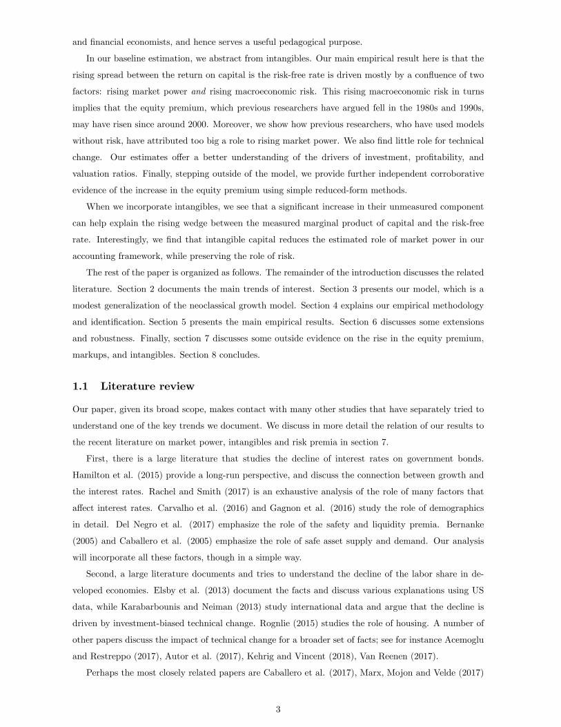
The top two panels of �gure 2 present measures of valuation ratios for the US stock market. The top
left panel shows the ratio of price to dividends from CRSP, while the top right panel shows the price-
operating earnings ratio for the SP500.2 The later is essentially trendless, while the former exhibits a
large boom and bust in 2000 before settling down to a higher value. Another commonly used valuation
ratio is the price-smoothed earnings ratio of Shiller (CAPE), which divides the SP500 price by a ten-year
moving average of real earnings, and is reported in table 1. While all these ratios are quite volatile,
overall they exhibit only a moderate increase from the �rst period to the second period. Our analysis
will emphasize that this limited increase is puzzling given the large decline of the risk-free rate (Fact
#1).
Fact #4: The share of investment in output or in capital has fallen slightly
The bottom two panels of �gure 2 depict the behavior of investment. As several authors have
noted recently (e.g. Eberly and Lewis (2016), Gutierrez and Philippon (2017)), investment has been
relatively lackluster over the past decade or more; but the magnitude of this decline is quite di¤erent
depending on how exactly one measures it. Because the price of investment goods falls relative to the
price of consumption goods, it is simpler to focus on the expenditure share of GDP (left panel) or
the ratio of nominal investment to capital (evaluated at current cost; right panel). Both ratios ought
2We focus on operating earnings which exclude exceptional items such as write-o¤s and hence are less volatile. In
particular, total earnings were negative in 2008Q4 because banks marked down the values of their assets substantially.
5

20
24
6
1985 1995 2005 2015
Shortterm real interest rate
02
46
8
1985 1995 2005 2015
Longterm real interest rate
24
68
10
1985 1995 2005 2015
Return to all capital (GRR)
1314
1516
17
1985 1995 2005 2015
Gross Profitability (our measure)
Figure 1: The top left panel displays the di¤erence between the 1-year Treasury bill rate and the median
1-year ahead CPI in�ation expectations from the Survey of Professional Forecasters (SPF). The top right
panel displays the di¤erence between the 10-year Treasury note rate and the median 10-year ahead CPI
in�ation expectations from the SPF. The bottom left panel presents the estimate of the pretax return on
all capital from Gomme, Ravikumar and Rupert (2011). The bottom right panel presents our measure of
gross pro�tability, the ratio of (1-labor share) to the capital-output ratio. The horizontal lines represent
the mean in the �rst and second half of the samples (1984-2000 and 2001-2016 respectively).
6

2040
6080
100
1985 1995 2005 2015
Pricedividend (CRSP)
1015
2025
30
1985 1995 2005 2015
SP 500 Priceoperating earnings
1416
1820
1985 1995 2005 2015
InvestmentGDP ratio6
78
910
1985 1995 2005 2015
Investmentcapital ratio
Figure 2: The top left panel displays the price-dividend ratio from CRSP. The top right panel shows
the ratio of price to operating earnings for the SP500. The bottom left panel is the ratio of nominal
investment spending to nominal GDP. The bottom right panel is the ratio of nominal investment to
capital (at current cost). The horizontal lines represent the mean in the �rst and second half of the
samples (1984-2000 and 2001-2016 respectively).
7

to be stationary in standard models, and they appear nearly trendless over long samples. Investment
spending exhibits a strong cyclical pattern, increasing faster than GDP during expansions and falling
faster than GDP during recessions, but overall both ratios appear to exhibit small to moderate declines
across our two subsamples. Table 1 also report the ratios for the nonresidential sector (i.e., business
�xed investment), which behaves very similarly, so our results are not driven by housing. Note that
business �xed investment include equipment, structures and intellectual property products. The table
also reports two measures of the evolution of the capital-output ratio; �rst, the ratio of capital at
current cost to GDP; and second, the ratio of a real index of capital services3 (from the BLS) to real
output.(which we normalize to one in 1984). Both ratios exhibit an increase of about 0.15.4
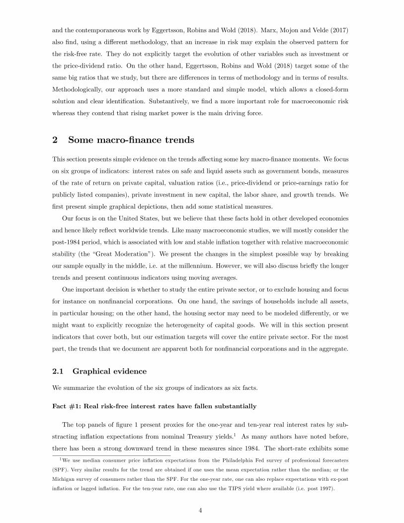
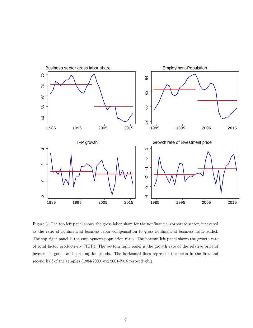
Fact #5: Total factor productivity and investment-speci�c growth have slowed down,
and the employment-population ratio has fallen
There has been much public discussion that overall GDP growth has declined over the past couple
of decades. This decline is in part attributable to a decline in the employment/population ratio, largely
due to demographic factors (Aaronson et al. (2015)), shown as the top right panel in Figure 3. However,
the decline in output per worker growth is still large between the two samples, from 1.8% per year to
1.2% per year according to table 1. This decline is largely driven by lower total factor productivity
(TFP) growth and lower investment-speci�c technical progress; Table 1 shows that the growth rate of
the Fernald TFP measure goes from 1.1% per year to less than 0.8% per year, while the growth rate of
the relative price of investment goods to nondurable and service consumption goes from -1.8% per year
to -1.1% per year; both are depicted in the bottom panels of Figure 3.
Fact #6: The labor share has fallen
Finally, the top left panel of �gure 3 presents a measure of the gross labor share for the non�nancial
corporate sector; table 1 includes a measure that covers the entire US economy. As has been noted by
many authors (e.g., Karabarbounis and Neiman (2013); Elsby et al. (2013); Rognlie (2015)), the labor
share exhibits a decline that is most clear after 2000 in the United States.
Of course, all of these facts are somewhat di¢ cult to ascertain graphically given the short samples
and the noise in some series. This leads us to evaluate next the statistical signi�cance of these changes.
2.2 Statistical evaluation
To summarize the trends in these series in a more formal way, Table 1 reports several statistics for the
series presented in �gures 1-3 above as well as for some alternative series that capture the same concepts.
Columns 1-4 report the means in the �rst and second subsamples, which are depicted in �gures 1-3 as
horizontal lines, together with standard errors. Column 5 reports the di¤erence between the means in
3This index aggregates underlying capital goods using rental prices, which is the correct measure for an aggregate
production function. In contrast, the capital at current cost is a nominal value which sums purchase prices.4Over the long term, these ratios do behave di¤erently, however. The BLS index exhibits an upward trend since the
mid 1970s due to the decline of the price of investment goods, but this trend has slowed down recently. In contrast, the
current cost capital/output ratio is nearly trendless.
8
6466
6870
72
1985 1995 2005 2015
Business sector gross labor share
5860
6264
1985 1995 2005 2015
EmploymentPopulation
20
24
1985 1995 2005 2015
TFP growth4
32
10
1
1985 1995 2005 2015
Growth rate of investment price
Figure 3: The top left panel shows the gross labor share for the non�nancial corporate sector, measured
as the ratio of non�nancial business labor compensation to gross non�nancial business value added.
The top right panel is the employment-population ratio. The bottom left panel shows the growth rate
of total factor productivity (TFP). The bottom right panel is the growth rate of the relative price of
investment goods and consumption goods. The horizontal lines represent the mean in the �rst and
second half of the samples (1984-2000 and 2001-2016 respectively).
9

the second and �rst sample, and column 6 is the associated standard error. Column 7 is the regression
coe¢ cient of the variable of interest on a linear time trend, and column 8 is the associated standard
error. (The standard errors are calculated using the Newey-West method with �ve (annual) lags.)
For some indicators, there is little evidence of a break between the samples, while for others, there is
overwhelming evidence of a break. Speci�cally, interest rates, the labor share, total factor productivity,
and the investment-capital ratios are markedly lower in the second sample. On the other hand, valuation
ratios and the return on capital appear fairly stable.
2.3 Longer historical trends
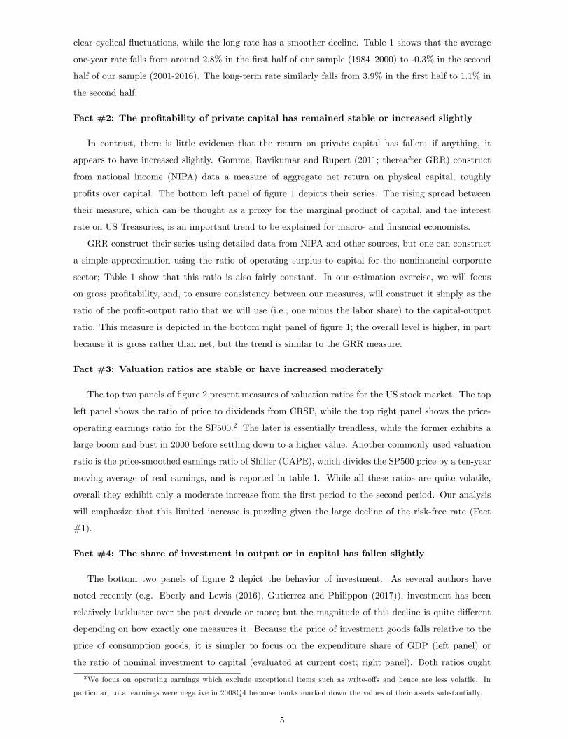
Figure 4 presents the evolution of nine of the moments we described above, but over a longer sample,
since 1950. (These nine moments will be our estimation target below.) For clarity, we add a 11�year
centered moving average to each series, so we depict the evolution from 1955 to 2011. One motivation
for studying a longer sample is that real interest rates were also low in the 1970s and to some extent
the 1960s, and hence one question is whether the abnormal period is the early 1980s when real interest
rates were very high. The �gure shows, however, that the analogy does not apply to all variables. It is
true that pro�tability was high in the 1960s, but the price-dividend ratio was lower, and the labor share
and the investment-capital ratio were relatively high, in contrast to the more recent period. Overall,
neither the 1960s nor the 1970s are similar in all respects to the post 2000 period. Moreover, a serious
consideration of the role of in�ation is warranted to study the 1970s and early 1980s, as in�ation likely
a¤ected many of the macroeconomic aggregates depicted here. This is why, for now, we focus on the post
1984 sample. But we will present some results below starting in 1950 to illustrate what our approach
implies for these earlier periods.
3 Model
This section introduces a simple macroeconomic model to account for the macro-�nance moments.
Our framework adds macroeconomic risk and monopolistic competition to a neoclassical growth model.
Given our focus on medium-run issues, we abstract from nominal rigidities and adjustment costs.
3.1 Model setup
We consider a standard dynastic model with inelastic labor supply. In order to highlight the role of risk,
we use Epstein-Zin preferences:
Vt = Lt
�(1� �)c1��pc;t + �Et
�V 1��t+1
� 1��1��
� 11��
; (1)
where Vt is utility, Lt is population size (which is exogenous and deterministic), cpc;t is per-capita
consumption at time t; � is the inverse of the intertemporal elasticity of substitution of consumption,
and � the coe¢ cient of relative risk aversion. We assume that labor supply is exogenous and equal to
Nt = NLt where N is a parameter that captures the employment-population ratio.
10

Group Variable Averages Trend
1984-�00 SE 2001-�16 SE Di¤. SE Coe¤. SE
Real interest rate One-year maturity* 2.79 .45 -.35 .59 -3.14 .75 -.17 .02
Ten-year maturity 3.94 .41 1.06 .46 -2.88 .69 -.18 .01
AA rate 4.69 .48 1.09 .57 -3.6 .8 -.21 .02
Ten-year adj. for term premium 1.52 .26 -.09 .35 -1.61 .4 -.08 .02
Return on capital GRR: all, pretax 6.1 .2 7.24 .45 1.14 .45 .07 .02
GRR: business, pretax 8.59 .32 10.46 .62 1.87 .62 .11 .03
Non�n. corps. GOS/NRK 7.59 .34 7.87 .36 .27 .51 .04 .01
Gross pro�tability* (see text) 14.01 .26 14.89 .49 .88 .6 .07 .02
Valuation ratios Price-dividend ratio* CRSP 42.34 8.56 50.11 3.4 7.78 8.39 .67 .36
Price-operating earnings SP500 18.7 2 18.31 1.09 -.39 1.75 .03 .12
Price-smoothed earnings Shiller 22.07 4.41 24.36 1.25 2.29 4.5 .33 .17
Investment Investment share in GDP 17.43 .53 16.93 .65 -.5 .76 -.04 .04
Nonres. invest. share in GDP 12.94 .40 12.79 .18 -.15 .43 0 .02
Investment-capital: all* 8.1 .25 7.23 .35 -.88 .38 -.04 .02
Investment-cap.: nonresidential 10.95 .39 10.2 .24 -.76 .4 -.03 .02
Capital-output Fixed asset 2.13 .03 2.28 .03 .15 .04 .01 0
Real index (BLS) 1.06 .02 1.18 .01 .13 .02 .01 0
Labor share Nonfarm business (BLS) gross 62.07 .31 58.56 1.01 -3.51 1.11 -.21 .04
Non�nancial corps. gross* 70.11 .34 66.01 1.21 -4.1 1.29 -.24 .05
Growth Output per worker 1.80 .22 1.22 .23 -.58 .29 -.03 .02
Total factor productivity* 1.10 .31 .76 .32 -.34 .36 -.02 .02
Population* 1.17 .08 1.1 .06 -.07 .08 0 0
Price of investment: all* -1.77 .15 -1.13 .34 .64 .26 .03 .02
Price of investment: nonresid. -2.38 .19 -1.75 .29 .63 .25 .04 .02
Price of invt: equipment -3.62 .60 -3.27 .53 .34 .72 .02 .04
Price of invt: IPP -1.71 .30 -2.15 .36 -.44 .52 0 .02
Employment-pop. ratio* 62.34 .58 60.84 0.94 -1.51 1.06 -.07 .06
Table 1: The table reports, for each variable, the mean in the sample 1984-2000, in the sample 2001-2016,
and the di¤erences of means, as well as the coe¢ cient on a linear time trend, all with standard errors.
Stars indicate moments targeted in our estimation exercise. GRR stands for Gomme, Ravikumar and
Rupert (2011), GOS for gross operating surplus, NRK for non-residential capital, and IPP for intellectual
property products. Variables construction detailed in appendix.
11

1 9 6 0 1 9 8 0 2 0 0 0
1 2
1 4
1 6
/K
1 9 6 0 1 9 8 0 2 0 0 0
2 8
3 0
3 2
3 4
3 6/Y
1 9 6 0 1 9 8 0 2 0 0 0
2
0
2
4
6
R is k fr e e r a te
1 9 6 0 1 9 8 0 2 0 0 02 0
4 0
6 0
8 0
P r ic e D iv id e n d
1 9 6 0 1 9 8 0 2 0 0 06
7
8
9
I /K
1 9 6 0 1 9 8 0 2 0 0 0
2
0
2
4T F P g r o w th
1 9 6 0 1 9 8 0 2 0 0 04
2
0
2
In v t P r ic e G ro w th
1 9 6 0 1 9 8 0 2 0 0 0
1
1 .5
2
2 .5
P o p u la tio n G r o w th
1 9 6 0 1 9 8 0 2 0 0 0
0 .5 6
0 .5 8
0 .6
0 .6 2
0 .6 4E m p /P o p
Figure 4: This �gure presents the nine series used in our estimation exercise over the 1955-2011 sample,
together with a 11�year centered moving average.
12

Final output is produced using constant return to scale from di¤erentiated inputs,
Yt =
�Z 1
0
y"�1"
it di
� ""�1
;
where " > 1 is the elasticity of substitution. These intermediate goods are produced using a Cobb-
Douglas production function,
yit = Ztk�it(Stnit)
1��;
where kit and nit are capital and labor in �rm i at time t, Zt is an exogenous deterministic productivity
trend, and St is a stochastic productivity process, which we assume to be a martingale:
St+1 = Ste�t+1 ; (2)
where �t+1 is iid.
Capital is accumulated using a standard investment technology, but is subject to an aggregate
�capital quality�shock t+1, which we also assume to be iid :
kit+1 = ((1� �) kit +Qtxit) e t+1 :
Here Qt is an exogenous deterministic process re�ecting investment-speci�c technical progress as in
Greenwood, Hercowitz, and Krusell (1997). The relative price of investment and consumption goods is
1=Qt:
Capital and labor can be reallocated frictionlessly across �rms at the beginning of each period after
the shocks � and have been realized. Given the constant-return-to-scale technology, �rms then face
a constant (common) marginal cost. It is easy to see (see appendix for details) that the economy
aggregates to a production function
Yt = ZtK�t (StNt)
1��; (3)
and that markups distort the �rms��rst order conditions, leading to
(1� �) YtNt
= �wt; (4)
�YtKt
= �Rt; (5)
where � = ""�1 > 1 is the gross markup, wt is the real wage and Rt the rental rate of capital.
Moreover, the law of motion for capital accumulation also aggregates,
Kt+1 = ((1� �)Kt +QtXt) e t+1 : (6)
The choice of investment is determined by the (common) marginal product of capital, leading to the
Euler equation:
Et�Mt+1R
Kt+1
�= 1; (7)
where Mt+1 is the real stochastic discount factor and RKt+1 is the return on capital, which is given by:
RKt+1 =
��Yt+1�Kt+1
+1� �Qt+1
�Qte
�t+1 : (8)
13
This expression is a standard user cost formula, which incorporates the rental rate of capital of equation
(5) but also depreciation, the price of investment goods, and the capital quality shock. Given the
preferences assumed in equation (1), the stochastic discount factor is
Mt+1 = �
�Lt+1Lt
�1�� �cpc;t+1cpc;t
��� Vpc;t+1
Et((Vpc;t+1)1��)
11��
!���; (9)
where Vpc;t is the utility per capita, Vpc;t = Vt=Lt:
The resource constraint reads
Ct +Xt = Yt; (10)
where Ct = Ltcpc;t is total consumption, and Xt are investment expenses measured in consumption
good units.
The equilibrium of this economy is�cpc;t; Ct; Xt;Kt; Yt; R
Kt+1;Mt+1; Vpc;t; Vt
that solve the system
of equations (1)-(10), given the exogenous processes�Lt; Zt; Qt; St; �t+1; t+1
: As is well known, such
a model admits in general no closed form solution. Many authors build their intuition by solving for the
nonstochastic steady-state. While useful, this obviously requires to abstract from macroeconomic risk,
This makes it di¢ cult to understand the role that macroeconomic risk may play, leading most authors
to rely on numerical approximations. We will show, in contrast, that for an interesting special case, our
model can be solved easily for a �risky balanced growth path�.
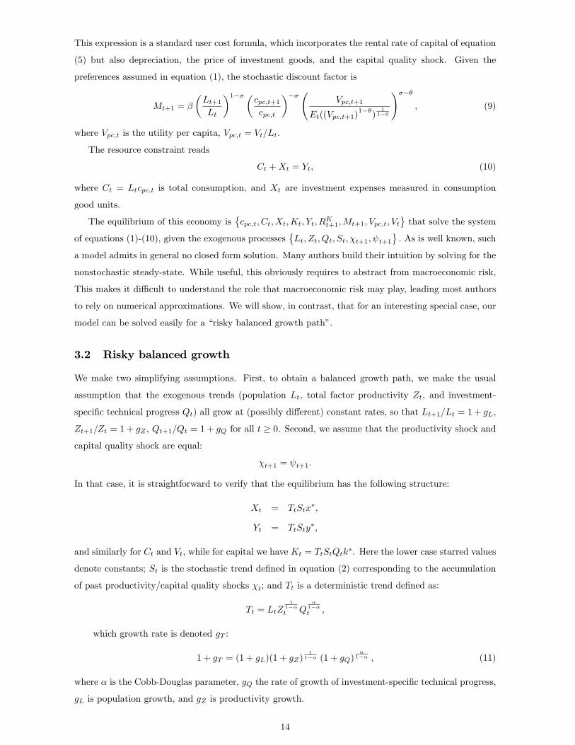
3.2 Risky balanced growth
We make two simplifying assumptions. First, to obtain a balanced growth path, we make the usual
assumption that the exogenous trends (population Lt, total factor productivity Zt, and investment-
speci�c technical progress Qt) all grow at (possibly di¤erent) constant rates, so that Lt+1=Lt = 1+ gL;
Zt+1=Zt = 1 + gZ ; Qt+1=Qt = 1 + gQ for all t � 0. Second, we assume that the productivity shock and
capital quality shock are equal:
�t+1 = t+1:
In that case, it is straightforward to verify that the equilibrium has the following structure:
Xt = TtStx�;
Yt = TtSty�;
and similarly for Ct and Vt, while for capital we have Kt = TtStQtk�. Here the lower case starred values
denote constants; St is the stochastic trend de�ned in equation (2) corresponding to the accumulation
of past productivity/capital quality shocks �t; and Tt is a deterministic trend de�ned as:
Tt = LtZ1
1��t Q
�1��t ;
which growth rate is denoted gT :
1 + gT = (1 + gL)(1 + gZ)1
1�� (1 + gQ)�
1�� ; (11)
where � is the Cobb-Douglas parameter, gQ the rate of growth of investment-speci�c technical progress,
gL is population growth, and gZ is productivity growth.
14

Finally, the stochastic discount factor is
Mt+1 = � (1 + gL) (1 + gT )��
e���t+1E(e(1��)�t+1)���1�� ;
where � is risk aversion and � the inverse of the IES. We can then easily calculate all objects of interest
in the model, including x�; y�; as we show in appendix.
Figure 5 presents an example of the time series produced by the model. The equilibrium corresponds
to a �balanced growth path�, but one where macroeconomic risk still a¤ects decisions and realizations.
Speci�cally, the realization of the macroeconomic shock �t+1 a¤ects the stochastic trend St+1 and
hence Xt+1; Yt+1; etc., while the e¤ect of risk, on the other hand, is re�ected in the constants x�; y�:
The bottom line is that the �big ratios�such as It=Yt; �t=Yt; �t=(Kt=Qt); etc. are constant, as in the
standard Kaldor calculations, but now incorporate risk; we discuss these ratios in the next section.5
This result holds regardless of the probability distribution of �t+1:
The treatment of deterministic trends is completely standard. What is less standard is that in our
model, a common stochastic trend a¤ect all variables equally, which generates great tractability. In
the standard RBC model, t+1 = 0; and then permanent productivity shock �t+1 leads to a transition
as the economy adjusts its capital stock to the newly desired level, before eventually reaching the new
steady-state. By assuming �t+1 = t+1; this transition period is eliminated because the capital stock
�miraculously�adjusts by the correct amount. This simpli�es the solution of the model because agents�
expectations of future paths are now easy to calculate.6 ,7 The capital quality shock is also important
if the economy is to generate a signi�cant equity premium, for it makes the return on capital volatile
rather than bounded below by 1� �:
3.3 Model implications
This section presents model implications for the �big ratios�and other key moments of interest along
the risky balanced growth path. We will present the Euler equation, which leads to a standard user cost
calculation, then discuss valuation ratios and rate of returns.
It is useful to de�ne the composite parameter
�� = Et(Mt+1e�t+1);
which equals
�� = �(1 + gL)(1 + gT )�� � E(e(1��)�t+1)
1��1�� ; (12)
and its rate of return version r� = 1=�� � 1 ' � log ��, which satis�es
r� ' �� gL + �gT + �1� 1=�1� � logE(e(1��)�t+1); (13)
5Of course, the economy can also exhibit transitional dynamics if its initial capital is too low or too high, before it
reaches the balanced growth path.6Since we will not study the actual responses to �t+1 shocks, there is little loss in this simpli�cation: what is key for
us is that agents regard the future as uncertain, and that bad realizations of �t+1 will have reasonable consequences (e.g.
a low return on capital), which lead agents ex-ante to adjust their choices (e.g. investment).7This argument (formulated in Gabaix (2011) and Gourio (2012)) can be applied to larger models; for instance see
Gourio, Kashyap and Sim (2018) or Isore and Szczerbowicz (2018) for New Keynesian models with disaster risk.
15

0 20 40 60 802
0
2
log
ycx
0 20 40 60 80Time
0.1
0
0.1%
RRF
Figure 5: The �gure presents an example of the time series generated by the model. Top panel: output,
consumption and investment (in log); bottom panel: return on capital and risk-free rate. In this example,
the economy is a¤ected by two realizations of � shocks, at t = 4 and t = 57:
where � = 1=� � 1 ' � log �:8 The parameter r� will turn out to equal in equilibrium the expected
return on capital, and to be a �su¢ cient statistic�to solve for the �big ratios�- that is, we do not need
to know �=�; �, �, or the distribution of �, but only r�.
3.3.1 Capital accumulation
To solve the model, we use the Euler equation (7), which along the risky balanced growth path reads
1
��=
�
�Q��k�
N
���11
1 + gQ+1� �1 + gQ
!; (14)
where Q� is the �level�of investment technical progress Qt, i.e. Qt = Q�(1 + gQ)t; so 1=Q� is the level
of the relative price of investment and consumption. This equation pins down k� and the capital-labor
ratio, and it generalizes the familiar condition of the neoclassical growth model to incorporate risk
through ��. We can rewrite this as the equality of the user cost of capital and marginal revenue:
1
Q�(r� + � + gQ) �
�
�
�k�
N�
���1; (15)
Equation (15) directly shows how higher market power or a higher required risky return lower the desired
capital-labor ratio.
To calculate the other big ratios, �rst note that Kt=Qt is the capital stock, evaluated at current cost.
The capital-output ratio is obtained from equation (15) as:
Kt=QtYt
� �
�
1
r� + � + gQ; (16)
8Here and thereafter, the ' signs re�ects the �rst-order approximation log(1 + x) ' x ' 1=(1� x).
16

and the investment-capital ratio isXt
Kt=Qt� gQ + gT + �; (17)
which re�ects the familiar balanced growth relation. Last, the investment-output ratio is obtained by
combining equations (17) and (16):Xt
Yt� �
�
gT + � + gQr� + � + gQ
: (18)
3.3.2 Income Distribution
The labor share (in gross value added) is, using equation (4):
sL =wtNtYt
=1� ��
; (19)
and hence the measured capital share is sK = 1 � sL =�+��1
� : This capital share can be decomposed
into a pure pro�t share, that rewards capital owners for monopoly rents, and a true capital remuneration
share, corresponding to rental payments to capital, i.e. sK = s� + sC ; with
s� =�� 1�
; (20)
and
sC =�
�: (21)
3.3.3 Valuation ratios
The �rm value is the present discounted value of the dividends Dt = �t�Xt: In equilibrium, this value
equals the value of installed capital plus monopolistic rents. Formally, the ex-dividend �rm value Pt
satis�es the standard recursion,
Pt = Et (Mt+1 (Pt+1 +Dt+1)) :
Given that the equilibrium is iid; the price-dividend ratio is constant, and satis�es the familiar Gordon
formula:P �
D� =1
1��(1+gT )
� 1� 1 + gTr� � gT
: (22)
Tobin�s Q isPt
Kt=Qt� 1 + �� 1
�
r� + � + gQr� � gT
: (23)
Because we do not incorporate adjustment costs, Tobin�s Q equals one when there is no market power,
i.e. � = 1: But if there is some market power, the value of Tobin�s Q depends on several parameters,
which a¤ect (i) the size of the economy and hence the rents, (ii) the discount rate applied to all future
rents.
17

3.3.4 Rates of Return
We now compare three benchmark rate of returns in this economy: the risk-free rate, the return on equity,
and the pro�tability of capital, which is often used in macroeconomics as a proxy for the marginal product
of capital. The gross risk-free rate (which can be priced even though it is not traded in equilibrium) is
RF =1
E(Mt+1)=E�e(1��)�t+1
���E
�e���t+1
� ;which we can rewrite as the net risk-free rate, i.e. rf = RF � 1 :
rf � r� + logE�e(1��)�t+1
�� logE
�e���t+1
�: (24)
The average pro�tability of capital can be inferred, as in Gomme, Ravikumar and Rupert (2011) and
Mulligan (2002), as the ratio of (measured) pro�ts to the stock of capital. This can be calculated either
gross or net of depreciation. For instance, in gross terms, we have
MPK =�t
Kt=Qt;
=�+ �� 1
�(r� + � + gQ) : (25)
Conceptually, this MPK excess the risk-free rate for three reasons; �rst, it is gross of both physical
and economic depreciation; second, it incorporates pro�t rents; third, it is risky. We can decompose the
spread between the MPK and the risk-free rate to re�ect these three components:
MPK � rf = � + gQ +�� 1�
(r� + � + gQ) + r� � rf : (26)
A main goal of our empirical analysis is to evaluate the importance of these di¤erent components in the
data.
The expected equity return is de�ned as
E (Rt+1) = E
�Pt+1 +Dt+1
Pt
�;
and it is easy to show using equation (22) that
E(Rt+1) =1
��E(e�t+1): (27)
In the case where E (e�t+1) = 1, which we will enforce in our applications, the gross expected return on
equity is exactly 1=��, and the net return is r�: The same expected return also applies the return on
physical capital RKt+1 =��Yt+1�Kt+1
+ 1��Qt+1
�Qte
�t+1 de�ned in equation (8). Conceptually, the �rm value
here stems from capital and rents, but it turns out that both components have equal risk exposure and
hence equal expected returns.
Finally, the equity risk premium ERP is obtained by combining equations (24) and (27):
ERP =E (Rt+1)
Rf;t+1=E�e���t+1
�E(e�t+1)
E�e(1��)�t+1
� :
18
3.4 Comparative statics
We now use the expressions developed in the previous section to illustrate some key comparative statics
of the risky balanced growth path. These comparative statics are useful to understand identi�cation of
our model. Most of the parameters have the usual e¤ects; we will focus on parameters that are typically
absent from the neoclassical growth model, or parameters that play an important role in our empirical
results.
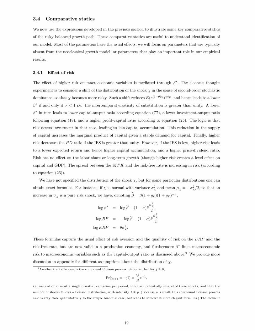
3.4.1 E¤ect of risk
The e¤ect of higher risk on macroeconomic variables is mediated through ��: The cleanest thought
experiment is to consider a shift of the distribution of the shock � in the sense of second-order stochastic
dominance, so that � becomes more risky. Such a shift reduces E(e(1��)�)1
1�� ; and hence leads to a lower
�� if and only if � < 1 i.e. the intertemporal elasticity of substitution is greater than unity. A lower
�� in turn leads to lower capital-output ratio according equation (??), a lower investment-output ratio
following equation (18), and a higher pro�t-capital ratio according to equation (25). The logic is that
risk deters investment in that case, leading to less capital accumulation. This reduction in the supply
of capital increases the marginal product of capital given a stable demand for capital. Finally, higher
risk decreases the PD ratio if the IES is greater than unity. However, if the IES is low, higher risk leads
to a lower expected return and hence higher capital accumulation, and a higher price-dividend ratio.
Risk has no e¤ect on the labor share or long-term growth (though higher risk creates a level e¤ect on
capital and GDP). The spread between the MPK and the risk-free rate is increasing in risk (according
to equation (26)).
We have not speci�ed the distribution of the shock �; but for some particular distributions one can
obtain exact formulas. For instance, if � is normal with variance �2� and mean �� = ��2�=2, so that an
increase in �� is a pure risk shock, we have, denoting b� = �(1 + gL)(1 + gT )��;
log �� = log b� � (1� �)��2�2;
logRF = � log b� � (1 + �)��2�2;
logERP = ��2�:
These formulas capture the usual e¤ect of risk aversion and the quantity of risk on the ERP and the
risk-free rate, but are now valid in a production economy, and furthermore �� links macroeconomic
risk to macroeconomic variables such as the capital-output ratio as discussed above.9 We provide more
discussion in appendix for di¤erent assumptions about the distribution of �:
9Another tractable case is the compound Poisson process. Suppose that for j � 0;
Pr(�t+1 = �jb) =�j
j!e��;
i.e. instead of at most a single disaster realization per period, there are potentially several of these shocks, and that the
number of shocks follows a Poisson distribution, with intensity � � p: (Because p is small, this compound Poisson process
case is very close quantitatively to the simple binomial case, but leads to somewhat more elegant formulas.) The moment
19

3.4.2 E¤ect of savings supply
A higher discount factor � has the same exact e¤ects as a decrease in risk (provided that the intertem-
poral elasticity is greater than unity) since its e¤ects are mediated through ��: Indeed, the only target
moment which is not a¤ected identically by both measures is the risk-free rate, which is a¤ected directly
by �� but also by risk aversion � or the quantity of risk �: Hence, higher savings supply leads to higher
capital accumulation, higher investment-output ratio and a lower marginal product of capital (re�ecting
higher supply of capital with stable demand), and a higher price-dividend ratio, while the risk-free rate
falls. The spread between the MPK and the risk-free rate, shown in equation (26) is little a¤ected by
�, only a¤ecting the quantity of rents through r�. The equity risk premium r�� rf is independent of �:
3.4.3 E¤ect of market power
One potentially important factor that has been invoked to explain of the trends we document is market
power. In our model, an increase in � has no e¤ect on long-term growth, the risk-free rate, or the
price-dividend ratio, but it has a signi�cant e¤ect on other variables. Higher markups reduce both
the labor share and the �true capital share�, that is, the share of national income devoted to the fair
(risk-adjusted) compensation of capital, but increases the pure pro�t share. According to equations (18)
and (??), higher market power reduces investment-output and capital-output ratios, as �rms have less
incentive to build capacity. The spread between the MPK and the risk-free rate is increasing in market
power (equation (26)). Finally, higher market power reduces the level of GDP.
3.4.4 E¤ect of trend growth
Trend growth gT - which can traced back to productivity growth, population growth, or investment-
speci�c technical growth �a¤ects �� but also a¤ects independently the ratios of interest. Higher growth
generally increases the investment-capital and investment-output ratios and increases the risk-free rate
and valuation ratios, while the e¤ect on pro�tability ratios depends on the exact source of growth.
4 Accounting framework
This section describes our empirical approach and discusses identi�cation.
4.1 Methodology
We use a simple method of moment estimation. In the interest of clarity and simplicity, we perform an
exactly identi�ed estimation with 9 parameters and 9 moments. In a �rst exercise, we estimate the model
generating function is �(x) = e��e�xb�1
�; and the objects of interest are:
log �� = log b� + 1� �1� �
��e�(1��)b � 1
�;
logRf = � log b� + � � �1� �
��e�(1��)b � 1
�� �
�e�b � 1
�;
logERP = ��e�b + e�b � e�(1��)b � 1
�:
It is straightforward to extend this calculation to the case of random size of shocks b, as in Kilic and Wachter (2017).
20
separately over our two samples: 1984-2000 and 2001-2016. We then discuss which parameters drive
variation in each moment. In a second exercise, we estimate the model over 11-year rolling windows,
starting with 1950�1961, and ending with 2006-2016. In all cases, we �t the model risky balanced growth
path to the model moments. In doing so, we abstract from business cycle shocks, in line with our focus
on longer frequencies.10
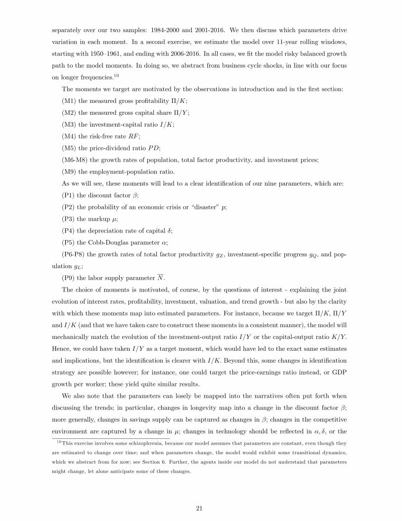
The moments we target are motivated by the observations in introduction and in the �rst section:
(M1) the measured gross pro�tability �=K;
(M2) the measured gross capital share �=Y ;
(M3) the investment-capital ratio I=K;
(M4) the risk-free rate RF ;
(M5) the price-dividend ratio PD;
(M6-M8) the growth rates of population, total factor productivity, and investment prices;
(M9) the employment-population ratio.
As we will see, these moments will lead to a clear identi�cation of our nine parameters, which are:
(P1) the discount factor �;
(P2) the probability of an economic crisis or �disaster�p;
(P3) the markup �;
(P4) the depreciation rate of capital �;
(P5) the Cobb-Douglas parameter �;
(P6-P8) the growth rates of total factor productivity gZ , investment-speci�c progress gQ, and pop-
ulation gL;
(P9) the labor supply parameter N:
The choice of moments is motivated, of course, by the questions of interest - explaining the joint
evolution of interest rates, pro�tability, investment, valuation, and trend growth - but also by the clarity
with which these moments map into estimated parameters. For instance, because we target �=K; �=Y
and I=K (and that we have taken care to construct these moments in a consistent manner), the model will
mechanically match the evolution of the investment-output ratio I=Y or the capital-output ratio K=Y:
Hence, we could have taken I=Y as a target moment, which would have led to the exact same estimates
and implications, but the identi�cation is clearer with I=K: Beyond this, some changes in identi�cation
strategy are possible however; for instance, one could target the price-earnings ratio instead, or GDP
growth per worker; these yield quite similar results.
We also note that the parameters can losely be mapped into the narratives often put forth when
discussing the trends; in particular, changes in longevity map into a change in the discount factor �;
more generally, changes in savings supply can be captured as changes in �; changes in the competitive
environment are captured by a change in �; changes in technology should be re�ected in �; �; or the
10This exercise involves some schizophrenia, because our model assumes that parameters are constant, even though they
are estimated to change over time; and when parameters change, the model would exhibit some transitional dynamics,
which we abstract from for now; see Section 6. Further, the agents inside our model do not understand that parameters
might change, let alone anticipate some of these changes.
21
growth rates of the technological factors gZ and gQ; etc. However, it is also possible that some economic
factors a¤ect all our parameters at the same time.
There are three parameters that we do not estimate; we discuss why, and how this a¤ects our
results in the next section on identi�cation. The three parameters are the elasticity of intertemporal
substitution 1=�; the coe¢ cient of risk aversion �, and the size of macroeconomic shocks b. Speci�cally,
we will assume that�t+1 follows a three-point distribution, i.e.
�t+1 = 0 with probability 1� 2p;
�t+1 = log(1� b) with probability p;
�t+1 = log(1 + bH) with probability p;
where bH is chosen so that E�e�+1
�= 1: We estimate p but �x b (and hence bH).
4.2 Identi�cation
In this section we provide a heuristic discussion of identi�cation, and make two main points. First, the
identi�cation is nearly recursive, so that it is easy to see which moments a¤ect which parameters. Second,
and consequently, the identi�cation of some parameters does not depend on all the data moments.
The identi�cation is easily seen to be nearly recursive. First, some parameters are obtained directly
as their counterparts are assumed to be directly observed: population growth, investment price growth
(the opposite of gQ), and the employment-population ratio. The growth rate gZ is next chosen to match
measured total factor productivity.11 One hence obtains gT , the trend growth rate of GDP, given by
equation (11). The depreciation rate � is then chosen to match I=K according to equation (17), which
is the familiar balanced growth relation:
I
K' � + gQ + gT :
The model then uses the Gordon growth formula (22) to infer the expected return on risky assets, r�
given the observed price-dividend ratio:
P �
D� '1 + gTr� � gT
:
Importantly, to infer r�; we do not need data on the risk-free rate or assumptions about, the value of
�; risk aversion �, or the distribution of �.
The next step is to identify the parameters � and � to match the pro�t share of output and the ratio
of pro�ts to capital using the equations (19) and (26). We solve for � and � are chosen to satisfy
sL =1� ��
;
11This step is however not straightforward, which is why we say that the identication is nearly recursive. TFP in the
data is measured using the revenue-based labor share, which in the model is sL = (1 � �)=�; rather than the cost-based
labor share, which in the model is 1� �: As a result, the TFP that an economist would measure in our model is
gT � sLgN � (1� sL)gK =
�sL
1� �gZ +
�sL�
1� �� (1� sL)
�gQ
�;
and hence is not equal to gZ since sL 6= 1� �: This turns out to have relatively small e¤ects in our empirical work.
22

and
MPK =�+ �� 1
�(r� + � + gQ) ;
where sL and MPK = �K are the observables.
The solution is, denoting by uc = r� + � + gQ the frictionless user cost, to set
� =MPK
sLMPK + (1� sL)uc;
and
� =uc(1� sL)
sLMPK + (1� sL)uc:
Intuitively, the �rst equation infers market power (here the Lerner index) by the magnitude of the
discrepancy between the MPK and the frictionless user cost of capital uc. The parameter � is then
obtained to �t the observed labor share. A key remark is that our identi�cation of � and � does not
require data on the risk-free rate or to make any assumption about risk aversion � or the distribution
of � - we simply use the su¢ cient statistic r� which has been previously identi�ed.
Economically, our approach boils down to using the traditional Gordon growth formula - which holds
in our standard neoclassical framework - to deduce the required return on capital from the price-dividend
ratio and the growth rate, and hence to construct a user cost of capital r� + � + gQ that incorporates
risk.12
At this point, we can also bring in data on the risk-free rate to infer the equity premium r��rf : Here
again, note that the behavior of the equity premium is therefore inferred without making assumptions
about risk aversion � or the distribution of �. However, to understand what drives the risk-free rate,
one needs to separately infer �, risk aversion �, and the quantity of risk �. Doing so requires extra
assumptions about these variables and about the intertemporal elasticity of substitution (which is not
identi�ed in our model given that growth rates are iid), as can be seen from equation (13):
r� ' �� gL + �gT + �1� 1=�1� � logE(e(1��)�t+1):
We present our baseline result with an IES of 2, a rare disaster distribution for � with a shock of
15% (eb = 0:85) and a probability p that we estimate, and a risk aversion coe¢ cient of 12. (In Section
6, we present the results when the IES is assumed to be 0.5 instead, and we also discuss results when
we choose other distributions for �, or if we instead �x the amount of risk and allow the risk aversion
coe¢ cient � to change.) As should be clear by now, none of these choices a¤ects our inferences about
�; �, or the equity premium.
Concretely, given these additional assumptions, we can solve for the quantity of risk p that satis�es
r� � rf = logE�e���t+1
�� logE
�e(1��)�t+1
�;
and we can then use the equation above for r� to �nd � i.e. �:
12Our procedure is closely related to the approach of Barkai (2016), the main di¤erence being the way we incorporate
risk. Barkai (2016) simply uses a treasury rate or corporate bond yield to construct the user cost.
23

Parameter name Symbol Estimates
1984-2000 2001-2016 Di¤erence
Discount factor � 0.955 0.967 0.012
Markup � 1.079 1.146 0.067
Disaster probability p 0.034 0.065 0.031
Depreciation � 2.778 3.243 0.465
Cobb-Douglas � 0.244 0.243 -0.000
Population growth gN 1.171 1.101 -0.069
TFP growth gZ 1.298 1.012 -0.286
Invt technical growth gQ 1.769 1.127 -0.643
Labor supply N 0.623 0.608 -0.015
Table 2: The table reports the estimated parameters in our baseline model for each of the two subsamples,
1984-2000 and 2001-2016, and the change between subsamples.
5 Empirical Results
We �rst compare the two subsamples, then we contrast the results with more standard macroeconomic
approaches which do not entertain a role for risk, and �nally we present results over rolling windows in
a long sample.
5.1 Comparison of two subsamples
Table 2 shows the estimated parameters for each subsample and the change of parameters between
subsamples. Overall, our results substantiate many of the narratives that have been advanced and
that we mention in the introduction. The discount factor � rises by 1.2 point, re�ecting higher savings
supply. Market power increases signi�cantly, by 6.7 points. Technical progress slows down and labor
supply falls (relative to population). The model also estimates a signi�cant increase in macroeconomic
risk (the probability of a crisis), which goes from 3.4% per year to 6.5% per year. We will return to
the interpretation of this result later. On the other hand, there is only moderate technological change:
depreciation increases, re�ecting the growing importance of high-depreciation capital such as computers,
but the Cobb-Douglas parameter remains fairly stable. This stability of the production function is an
interesting result. Overall, the model gives some weight to four of the most popular explanations
(�; �; p; gs): But exactly how much does each story explain?
Table 3 provides one answer. By construction, the model �ts perfectly all nine moments in each
subsample using the nine parameters . We can decompose how much of the change in each moment
between the two subsamples is accounted for by each parameter. Because our model is nonlinear, this
is not a completely straightforward task; in particular, when changing a parameter from �rst subsample
value to second subsample value, the question is at which value to evaluate the other parameters (e.g.,
24

the �rst or second subsample value). If the model were linear, or the changes in parameters small, this
would not matter, but such is not the case here (in particular for the price-dividend ratio, which is highly
nonlinear). In this table, we simply report the average over all possible orders of changing parameters,
as we move from the �rst to the second subsample.13
Overall, we see that the decline in the risk-free rate of 3.1% (314bps) is explained mostly by two
factors, higher perceived risk p, and higher savings supply �; with lower growth playing only a moderate
role.14 Why does the model not attribute all the change in the risk-free rate to savings supply? Simply
because it would make it impossible to match other moments, in particular the PD ratio. Even as it is,
if only the change in savings supply � were at work, the PD ratio would increase by nearly 32 points.
The model attributes o¤setting changes to risk and growth, explaining in this way that the PD ratio
increased only moderately over this period despite the lower interest rates.
Similarly, pro�tability would decrease by about 2 points if the change in � was the only one at work
- all rate of returns ought to fall if the supply of savings increases. The model reconciles the stable
pro�tability with the data by inferring higher markups and higher risk. Overall, we see how the model
needs multiple forces to account for the lack of changes observed in some ratios. The higher capital
share, is attributed entirely to higher markups, as capital-biased technical change appears to play little
role.
We can now use these model estimates to understand the evolution of some other moments; these
are reported in 4. First, as we discussed in Section 3 (equation 26), the spread between the marginal
product of capital and the risk-free rate can be decomposed in three components:
MPK � rf = � + gQ +�� 1�
(r� + gQ + �) + r� � rf ;
where the three components are depreciation (� + gQ), rents, and risk (r� � rf ). We can calculate
this decomposition in the model using the estimated parameters. The table reveals that depreciation
13Formally, let �a =��a1 ; :::�
aK
�and �b =
��b1; :::�
bK
�denote the parameter vectors in subsample a and b respectively,
and consider a model moment which is a function of the parameters: m = f(�): Consider a permutation � : [1;K]! [1;K]
that describes an order in which we change parameters from their initial to �nal value; we �rst change ��(1); then ��(2);
etc. Then calculate the change implied when we change parameter l 2 [1;K], i.e.
�l(�) = f(�bz2; �a�z2 )� f(�
bz1; �a�z1 ):
where z2 = �(1 : ��1(l)) and z1 = �(1 : ��1(l)� 1). The change in m due to parameter l 2 [1;K] is de�ned as
�l =1
N�
X�
�l(�);
where the sum ranges over all permutations. By construction,PKl=1�l = f(�b)� f(�a) accounts exactly for the model
implied change in the moment, which, because the model �ts the target moments perfectly, accounts also exactly for the
change in the data: f(�b)� f(�a) = mb �ma:
In table ?? in appendix, we report the upper and lower bounds when consider all possible combinations of other
parameters. This provides a way to bound the importance of each factor. We thank Sam Schulhofer-Wohl for these
suggestions. See Gourio (2018) for more details.
14This conclusion does depend somewhat on our assumed intertemporal elasticity of substitution, as we discuss in detail
below.
25
Target Moment Contribution of each parameter to change in moment
1984-00 2001-16 Di¤. � � p � � gN gZ gQ N
Gross pro�tability 14.01 14.89 0.88 -1.94 2.76 0.76 0.68 0.00 0.05 -0.29 -1.15 -0.00
Measured cap. share 29.89 33.99 4.10 -0.00 4.13 -0.00 0.00 -0.03 -0.00 0.00 -0.00 -0.00
Risk-free rate 2.79 -0.35 -3.14 -1.25 0.00 -1.62 0.00 -0.00 0.03 -0.19 -0.10 0.00
Price-dividend ratio 42.34 50.11 7.78 31.89 0.00 -13.34 0.00 -0.02 -2.82 -5.13 -2.80 0.00
Investment-capital 8.10 7.23 -0.88 0.00 -0.00 0.00 0.47 -0.00 -0.07 -0.39 -0.88 -0.00
Growth of TFP 1.10 0.76 -0.34 -0.00 -0.14 0.00 0.00 -0.00 -0.00 -0.26 0.06 0.00
Growth of invt. price -1.77 -1.13 0.64 0.00 0.00 0.00 0.00 0.00 0.00 0.00 0.64 0.00
Growth population 1.17 1.10 -0.07 0.00 0.00 0.00 0.00 0.00 -0.07 0.00 0.00 0.00
Employment-pop. 62.3 60.8 -1.50 0.00 0.00 0.00 0.00 0.00 0.00 0.00 0.00 -1.50
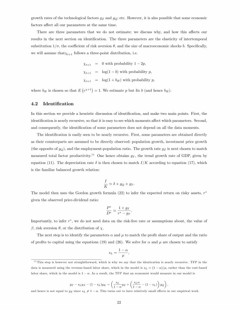
Table 3: The table reports the target moments in each of the two subsamples 1984-2000 and 2001-2016,
as well as the change between samples, and the contribution of each parameter to each change in moment
(so that column 3 equals the sum of columns 4 to 12). See text for details.
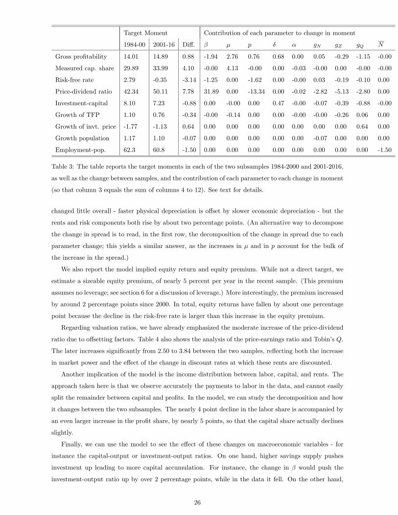
changed little overall - faster physical depreciation is o¤set by slower economic depreciation - but the
rents and risk components both rise by about two percentage points. (An alternative way to decompose
the change in spread is to read, in the �rst row, the decomposition of the change in spread due to each
parameter change; this yields a similar answer, as the increases in � and in p account for the bulk of
the increase in the spread.)
We also report the model implied equity return and equity premium. While not a direct target, we
estimate a sizeable equity premium, of nearly 5 percent per year in the recent sample. (This premium
assumes no leverage; see section 6 for a discussion of leverage.) More interestingly, the premium increased
by around 2 percentage points since 2000. In total, equity returns have fallen by about one percentage
point because the decline in the risk-free rate is larger than this increase in the equity premium.
Regarding valuation ratios, we have already emphasized the moderate increase of the price-dividend
ratio due to o¤setting factors. Table 4 also shows the analysis of the price-earnings ratio and Tobin�s Q.
The later increases signi�cantly from 2.50 to 3.84 between the two samples, re�ecting both the increase
in market power and the e¤ect of the change in discount rates at which these rents are discounted.
Another implication of the model is the income distribution between labor, capital, and rents. The
approach taken here is that we observe accurately the payments to labor in the data, and cannot easily
split the remainder between capital and pro�ts. In the model, we can study the decomposition and how
it changes between the two subsamples. The nearly 4 point decline in the labor share is accompanied by
an even larger increase in the pro�t share, by nearly 5 points, so that the capital share actually declines
slightly.
Finally, we can use the model to see the e¤ect of these changes on macroeconomic variables - for
instance the capital-output or investment-output ratios. On one hand, higher savings supply pushes
investment up leading to more capital accumulation. For instance, the change in � would push the
investment-output ratio up by over 2 percentage points, while in the data it fell. On the other hand,
26

rising market power and rising risk push investment down. Our model hence accounts for the coexistence
of low investment and low interest rates. Note also that higher depreciation also requires more investment
along the balanced growth path, while lower growth implies less investment. The model hence produces
a fairly nuanced decomposition for the evolution of this ratio.
Last, we can ask what is the e¤ect of each parameter on the level of GDP or investment.15 For
instance, higher market power discourages capital accumulation and reduces output. It is easy to show
that the elasticity of GDP to markups in this model is ��=(1 � �); or �0:32 for our estimate. Given
estimated markups rise by 6.2 percent (=6.7/1.079), the e¤ect on GDP is about �0:32� 6:2; or about
minus two percentage points (-1.95% in our table). Here too, there are several counteracting factors,
however, which imply that the overall level e¤ect on GDP is small (-0.30%). In particular, higher savings
supply and lower economic depreciation lead to higher capital accumulation, while higher risk leads to
lower capital accumulation. Investment is more negatively a¤ected by the changes, with a level e¤ect
of about minus 5 percentage points, owing largely to markups and risk, but also to lower growth and a
lower employment-population ratio.
5.2 Comparison with macroeconomic approaches
It is interesting to compare our results with alternative procedures followed by macroeconomists. Indeed,
our empirical exercise is essentially the calibration of the �steady-state�of a very bare-bone DSGEmodel.
Any DSGE model writer faces the same issues we do to �t these key moments.
Indeed, real business cycle modelers are aware of a trade-o¤ between �tting the capital-output ratio
and the risk-free interest rate. Since these models target the labor share, the discrepancy precisely re�ects
the gap between the MPK (pro�tability, or pro�t-capital ratio) and the risk-free interest rate. Often,
modelers reject short-term Treasury interest rates as measures of the rate of return on capital, noting
that these securities have special safety and liquidity attributes, which are not explicitly modeled.16
Mechanically, these models consider that the observed risk-free rate equals the model risk-free rate
times an unobserved convenience yield e�. This yields an additional parameter � to estimate. At the
same time, these models have traditionally abstracted from aggregate market power, setting � = 1;17
and from risk, so that p = 0, and have not explicitly targeted the price-dividend ratio. The assumptions
lead to a well-de�ned exactly identi�ed exercise with eight moments (baseline minus the price-dividend
ratio) and eight parameters (baseline plus the liquidity wedge �, less market power � and risk p), which
is an alternative to our approach. The last two columns of Table 5 present the results from this exercise,
which we call the �macro-without-markups�approach.15By level of GDP we mean y�; i.e. the level of GDP once the proper deterministic and stochastic trends have been
removed. We abstract from the growth e¤ects - e.g., a higher gZ or gQ has the mechanical e¤ect of steepening the overall
path of GDP.16See for instance Campbell et al. (2017) for a presentation of the Chicago Fed DSGE model, which, based on Fisher
(2015), introduces a liquidity wedge that accounts for the discrepancy between the risk-free rate and the rate of return of
capital.17New Keynesian models are an important exception, but market power is often set on a priori basis in these studies
(e.g., a markup of 15%), and pro�ts are o¤set in steady-state by �xed costs.
27
Model implied moments Contribution of each parameter
1984-00 2001-16 Di¤. � � p � � gN gZ gQ N
A. MPK-RF spread
Total spread 11.22 15.24 4.02 -0.68 2.76 2.39 0.68 0.00 0.02 -0.10 -1.05 0.00
- Depreciation 4.55 4.37 -0.18 0.00 0.00 0.00 0.47 0.00 0.00 0.00 -0.64 0.00
- Market power 3.39 5.55 2.17 -0.60 2.73 0.24 0.21 0.00 0.02 -0.09 -0.35 0.00
- Risk premium 3.15 5.23 2.08 -0.05 0.00 2.14 0.00 -0.00 0.00 -0.01 -0.00 0.00
B. Rate of returns
Equity return 5.85 4.90 -0.96 -1.25 0.00 0.56 0.00 -0.00 0.03 -0.19 -0.10 0.00
Equity premium 3.07 5.25 2.18 0.00 0.00 2.18 0.00 0.00 0.00 0.00 0.00 0.00
Risk-free rate 2.79 -0.35 -3.14 -1.25 0.00 -1.62 0.00 -0.00 0.03 -0.19 -0.10 0.00
C. Valuation ratios
Price-dividend 42.34 50.11 7.78 31.89 0.00 -13.34 0.00 -0.02 -2.82 -5.13 -2.80 0.00
Price-earnings 17.85 25.79 7.94 10.54 5.11 -4.62 -0.35 0.00 -0.92 -1.49 -0.36 0.00
Tobin�s Q 2.50 3.84 1.34 1.09 1.35 -0.48 0.11 0.00 -0.12 -0.28 -0.32 0.00
D. Income shares
Share Labor 70.11 66.01 -4.10 0.00 -4.13 0.00 0.00 0.03 0.00 0.00 0.00 0.00
Share Capital 22.59 21.24 -1.35 0.00 -1.33 0.00 0.00 -0.03 0.00 0.00 0.00 0.00
Share Pro�t 7.30 12.76 5.46 0.00 5.46 0.00 0.00 0.00 0.00 0.00 0.00 0.00
E. Macroeconomy
K/Y 2.13 2.28 0.15 0.30 -0.13 -0.12 -0.11 -0.00 -0.01 0.05 0.18 -0.00
I/Y 17.28 16.50 -0.78 2.26 -1.03 -0.90 0.23 -0.02 -0.22 -0.52 -0.59 -0.00
Detrend Y (% chg) � � -0.30 4.30 -1.95 -1.70 -1.52 -0.07 -0.12 0.65 2.56 -2.45
Detrend I (% chg) � � -4.95 17.67 -8.02 -6.98 -0.13 -0.20 -1.43 -2.45 -0.96 -2.45
Table 4: The table reports some moments of interest calculated in the model using the estimated
parameter values for each of the two subsamples 1984-2000 and 2001-2016, as well as the change between
samples, and the contribution of each parameter to each moment change.
28
Baseline approach Macro-with-markups Macro-without-markups
1984-00 2001-2016 Di¤. 1984-00 2001-2016 Di¤. 1984-00 2001-2016 Di¤.
� 0.955 0.967 0.012 0.978 1.007 0.028 0.935 0.928 -0.007
� 1.079 1.146 0.067 1.165 1.330 0.166 1 1 0
p 0.034 0.065 0.031 0 0 0 0 0 0
� 2.778 3.243 0.465 2.778 3.243 0.465 2.778 3.243 0.465
� 0.244 0.243 -0.000 0.183 0.122 -0.061 0.347 0.384 0.036
gP 1.171 1.101 -0.069 1.171 1.101 -0.069 1.171 1.101 -0.069
gZ 1.298 1.012 -0.286 1.544 1.358 -0.187 0.877 0.615 -0.262
gQ 1.769 1.127 -0.643 1.769 1.127 -0.643 1.769 1.127 -0.643
N 62.344 60.838 -1.507 62.344 60.838 -1.507 62.344 60.838 -1.507
� 0 0 0 0 0 0 -0.045 -0.082 -0.036
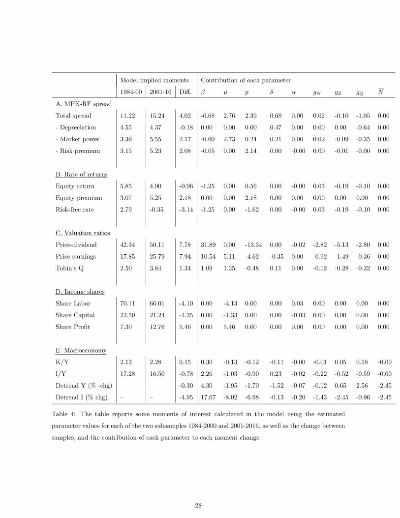
Table 5: The table reports the estimated parameters in each of the two subsamples 1984-2000 and
2001-2016 in our baseline model, in the macro model with markups, and in the macro model without
markups.
This approach leads to a much higher value of � and �explains�the decline of the labor share by an
increase of �: The decline of the Treasury rate, and the growing gap between the MPK and this rate,
are fully accounted for by a very large, and growing, liquidity premium, which equals �� = 4:5 percent
in the �rst sample and 8.2 percent in the second sample. We �nd both the level and increase in this
wedge implausible.
An alternative approach is to abstract from this liquidity but to allow for markup, while still omitting
the PD ratio from the list of targets and risk from the potential parameters. This is also a well-posed
exercise with 8 moments and 8 parameters which we call the �macro-with-markups�approach. In this
case, the spread between the MPK and the risk-free rate must re�ect depreciation or rents. Intuitively,
this approach assumes that the risk-free rate can be used to infer the cost of capital, and hence rents are
deduced as a residual. The approach is conceptually quite similar to Barkai (2016), though we present
it in a slightly more structural framework. The results are shown in the middle two columns of table
5. There are a number of di¤erences between these results and our baseline results. First, the level of
markups is much higher, and the increase in markups is much stronger (16.6 points instead of 6.7 points).
Second, the increase in markups is so large that the model requires a sharp decline in � (from 0.18 to
0.12) to keep the labor share from falling too much. This estimate suggests that technical progress has
been biased towards labor over the past thirty years - a somewhat implausible conclusion. On the other
hand, this model also implies that � rose signi�cantly. We will show some further di¤erences for a longer
sample below.
Table 6 presents the implications of these di¤erent �calibrations�. Notably, our approach o¤ers a
balanced view where markups and risk premia increases jontly explain the rising spread, while the
29

macro model without markups accounts all of it with an unmodeled liquidity premium and the macro
model with markups accounts for all of it with rising market power. As a result, that the macro model
with markups implies a sharp decline of the level of GDP, by about 8 percentage points. Moreover, the
share of income going to capital falls sharply, in opposite to the share of pro�ts which surges. On the
other hand, the macro model without markups predict an increase in the level of GDP relative to trend,
owing to the lower economic depreciation and higher incentives for capital accumulation.
Another interesting implication is that Tobin�s Q, which increase signi�cantly in our baseline, in
a way broadly consistent with the data, is actually unde�ned in the macro-with-markups approach,
because the low discount rates make the �rm value in�nite. In this sense, that model cannot match the
evolution of valuation ratios, given its target of interest rates. Furthermore, the macro-without-markups
approach implies decreasing valuation ratios, at odds with the data, owing to the very large, and rising,
liquidity premium. These results provide indirect support for our baseline model.
5.3 Rolling estimation
An alternative approach to �tting the model is to estimate it using rolling windows rather than two
subsamples. In this spirit, �gure 6 presents the estimated parameters when we estimate the model each
year using a 11�year centered moving average to calculate the target moments. (That is, we target the
smooth lines shown in Section 2 in �gure 4.) We start our analysis in 1950 to avoid World War II.18 As
noted above, this calculation assumes that agents are myopic, in the sense that they believe that the
currently observed target moments will be constant forever, and it abstracts from transitional dynamics.
We �nd a U shape in the parameter � (savings supply) and in macroeconomic risk p: Markups also
have a U shape but also an initial increase in the 1950s and 1960s. The capital parameter � has an
increase in the late 1970s which is later reversed. Figure 7 compares the evolution of our parameters
�; � to the parameters estimated using the �macro with markups�approach. Our estimated parameters
are signi�cantly more stable over time. We �nd this interesting because accounting for stock market
valuation ratios might be expected to lead to more unstable parameters - but we �nd the opposite.
We can then use these rolling estimates to study the income distribution, the return spread MPK�
RF; and their drivers. Figure 8 presents the share of pure pro�ts, the true capital share, and the sum
of the two for each year. By construction, the total equals one minus the labor share, and matches the
data exactly.
The �gure shows that the share of pure pro�ts is estimated to have risen in the 1960s, then falling in
the 1970s and rising since 1980. Inversely, the capital share fell, then rose and fell. This picture re�ects
the puzzling pattern of U shape in pro�ts and inverse U shape in � emphasized by Karabarbounis and
Neiman (2018). However, we �nd it interesting that the U shape is signi�cantly less strong with our
estimation strategy than if one follows the macro with markups strategy. Karabarbounis and Neiman
(2018) note that the strong negative correlation between the interest rate and the capital share, and the
strong positive correlation between the interest rate and the pro�t share, are suggestive of measurement
18We thank Matthew Rognlie for proposing (and executing) this exercise in his discussion at the NBER Summer Institute.
30
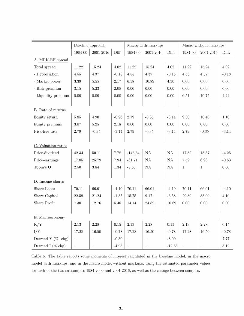
Baseline approach Macro-with-markups Macro-without-markups
1984-00 2001-2016 Di¤. 1984-00 2001-2016 Di¤. 1984-00 2001-2016 Di¤.
A. MPK-RF spread
Total spread 11.22 15.24 4.02 11.22 15.24 4.02 11.22 15.24 4.02
- Depreciation 4.55 4.37 -0.18 4.55 4.37 -0.18 4.55 4.37 -0.18
- Market power 3.39 5.55 2.17 6.58 10.89 4.30 0.00 0.00 0.00
- Risk premium 3.15 5.23 2.08 0.00 0.00 0.00 0.00 0.00 0.00
- Liquidity premium 0.00 0.00 0.00 0.00 0.00 0.00 6.51 10.75 4.24
B. Rate of returns
Equity return 5.85 4.90 -0.96 2.79 -0.35 -3.14 9.30 10.40 1.10
Equity premium 3.07 5.25 2.18 0.00 0.00 0.00 0.00 0.00 0.00
Risk-free rate 2.79 -0.35 -3.14 2.79 -0.35 -3.14 2.79 -0.35 -3.14
C. Valuation ratios
Price-dividend 42.34 50.11 7.78 -146.34 NA NA 17.82 13.57 -4.25
Price-earnings 17.85 25.79 7.94 -61.71 NA NA 7.52 6.98 -0.53
Tobin�s Q 2.50 3.84 1.34 -8.65 NA NA 1 1 0.00
D. Income shares
Share Labor 70.11 66.01 -4.10 70.11 66.01 -4.10 70.11 66.01 -4.10
Share Capital 22.59 21.24 -1.35 15.75 9.17 -6.58 29.89 33.99 4.10
Share Pro�t 7.30 12.76 5.46 14.14 24.82 10.69 0.00 0.00 0.00
E. Macroeconomy
K/Y 2.13 2.28 0.15 2.13 2.28 0.15 2.13 2.28 0.15
I/Y 17.28 16.50 -0.78 17.28 16.50 -0.78 17.28 16.50 -0.78
Detrend Y (% chg) � � -0.30 � � -8.00 � � 7.77
Detrend I (% chg) � � -4.95 � � -12.65 � � 3.12
Table 6: The table reports some moments of interest calculated in the baseline model, in the macro
model with markups, and in the macro model without markups, using the estimated parameter values
for each of the two subsamples 1984-2000 and 2001-2016, as well as the change between samples.
31
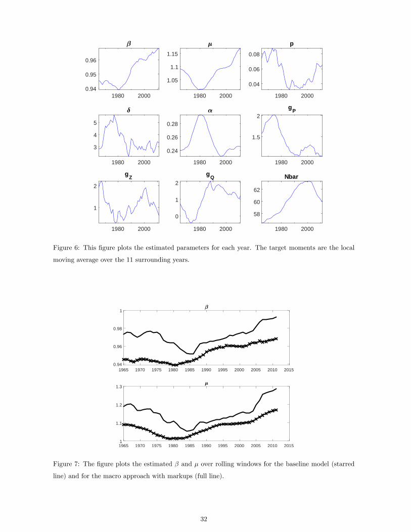
1980 20000.94
0.95
0.96
1980 2000
1.05
1.1
1.15
1980 2000
0.04
0.06
0.08
p
1980 2000
3
4
5
1980 2000
0.24
0.26
0.28
1980 2000
1.5
2gP
1980 2000
1
2
gZ
1980 2000
0
1
2gQ
1980 2000
58
60
62
Nbar
Figure 6: This �gure plots the estimated parameters for each year. The target moments are the local
moving average over the 11 surrounding years.
1965 1970 1975 1980 1985 1990 1995 2000 2005 2010 20150.94
0.96
0.98
1
1965 1970 1975 1980 1985 1990 1995 2000 2005 2010 20151
1.1
1.2
1.3
Figure 7: The �gure plots the estimated � and � over rolling windows for the baseline model (starred
line) and for the macro approach with markups (full line).
32

1965 1970 1975 1980 1985 1990 1995 2000 2005 20100
5
10
15
20
25
30
35Decomposition of income
capital+rentscapitalrents
Figure 8: This �gure presents the model-implied distribution of income, using the parameters estimated
in each year using the rolling window estimation. The labor share is one minus the sum of capital and
rents.
problems in the cost of capital. Figure 9 shows the capital share and the pure pro�t share implied by
the two estimations. There is clearly less volatility of the macro-�nance estimates.
Figure 10 presents the MPK � RF spread and its three subcomponents: economic and physical
depreciation, rents, and risk. The spread falls in the 1970s before rising in the 1980s. The depreciation
component moves, if anything, in opposite direction to the spread, and hence does not help explain its
movements. Rents are estimated to fall then rise, and so does risk. The empirical success here is that
the risk premium - which is estimated without looking at the MPK, but rather by single-mindedly
observing the PD ratio - helps explain some of this variation.
Figure 11 again compares these results to those obtained with the more standard macro estimation.
Both estimation approaches infer the same depreciation component. The macro approach attributes
none of the spread to risk by construction and hence infers a large and highly volatile rent (or pro�t)
component. Finally, �gure 12 depicts the implied risk-free rate, equity return and equity risk premium.
The risk-free rate exactly matches our data target by construction. The equity premium mimics the
evolution of p depicted in �gure 6.
6 Extensions and robustness
This section presents some extensions of our baseline framework. We �rst discuss the interpretation of
rising risk premia and alternative approaches to modeling them. We next analyze how �nancial leverage,
the intertemporal elasticity of substitution, alternative interest rates that adjust for liquidity or term
premia, and capital mismeasurement a¤ect our results. Finally, we present an example to evaluate the
33
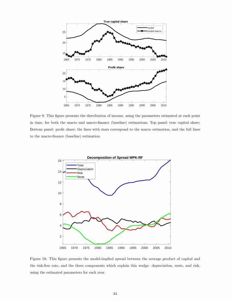
1965 1970 1975 1980 1985 1990 1995 2000 2005 2010
15
20
25
True capital share
modelmodelmacro
1965 1970 1975 1980 1985 1990 1995 2000 2005 2010
5
10
15
20
Profit share
Figure 9: This �gure presents the distribution of income, using the parameters estimated at each point
in time, for both the macro and macro-�nance (baseline) estimations. Top panel: true capital share;
Bottom panel: pro�t share; the lines with stars correspond to the macro estimation, and the full lines
to the macro-�nance (baseline) estimation.
1965 1970 1975 1980 1985 1990 1995 2000 2005 2010
2
4
6
8
10
12
14
16Decomposition of Spread MPKRF
TotalDepreciationRiskRents
Figure 10: This �gure presents the model-implied spread between the average product of capital and
the risk-free rate, and the three components which explain this wedge: depreciation, rents, and risk,
using the estimated parameters for each year.
34
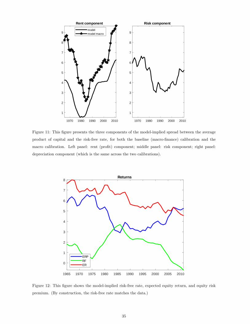
1970 1980 1990 2000 2010
1
2
3
4
5
6
7
8
9
Rent component
modelmodel macro
1970 1980 1990 2000 2010
1
2
3
4
5
6
7
8
9
Risk component
Figure 11: This �gure presents the three components of the model-implied spread between the average
product of capital and the risk-free rate, for both the baseline (macro-�nance) calibration and the
macro calibration. Left panel: rent (pro�t) component; middle panel: risk component; right panel:
depreciation component (which is the same across the two calibrations).
1965 1970 1975 1980 1985 1990 1995 2000 2005 2010
0
1
2
3
4
5
6
7
8Returns
ERPRFER
Figure 12: This �gure shows the model-implied risk-free rate, expected equity return, and equity risk
premium. (By construction, the risk-free rate matches the data.)
35

importance of transitional dynamics.
6.1 Interpretation of rising risk premia
Our baseline results are obtained using a parametrization of � as a rare �disaster� corresponding to
a permanent decline of 15% of the level of GDP. Our estimates suggest that the risk of such a large
shock was low in the 1990s but rose gradually in the 2000s and 2010s. Part of this increase may be
attributed to a recognition post 2008 that �nancial crises are recurrent events that a¤ect even developed
economies.19 But part of this increase occurs before the �nancial crisis. One interpretation is that this
increase corresponds to a higher perception of risk starting in the late 1990s and early 2000s owing
to the combination of the Asian �nancial crisis, LTCM crisis, and the 2001 crash in the US. We must
acknowledge however that it is not straightforward to relate our estimate of the probability of a �disaster�
to actual beliefs.20 This leads us to consider alternative interpretation, such as the ageing of developed
economies, or the desire of emerging markets to accumulate safe reserves, both of which might be
interpreted in a reduced form as higher e¤ective risk aversion.
As explained in section 4.2, the precise speci�cation of the risk model is theoretically irrelevant for
some conclusions, such as the value of markups � or the Cobb-Douglas parameter �, or the estimated
equity premium ERP:We now illustrate that even for the objects where this speci�cation is potentially
relevant, it may not be quantitatively �rst-order. Table 7 presents estimates of parameters in the �rst
and second samples under some alternative modeling of risk. The �rst row presents the baseline model.
The second and third row present alternative disaster models where, rather than a �bonanza�or windfall
to o¤set the disaster risk, we introduce a small positive drift or do not o¤set the disaster. The results
are nearly identical. Row four considers a log-normal process for � rather than a rare disaster. That
model requires a large, and rising, standard deviation �� of the lognormal shock to account for the data,
but as we will see, it behaves quite similarly overall. Rows 5 and 6 show estimates when the disaster
size b (resp. risk aversion �), rather than the disaster probability, is allowed to vary. Unsurprisingly,
these models require rising disaster size or risk aversion to account for the data. But all of these models
generate a perfect �t of the data moments. Finally, rows 7 and 8 present estimates of the baseline model
when the IES is set to unity or half rather than two; we discuss these below.
Table 8 present the �causal� decomposition along the lines of Tables 3 and 4, i.e. they show the
e¤ect of the changes in �, the risk parameter used in the variant (p; �,b or ��), or the other parameters
(all grouped together for simplicity) on some model moments. We know already that the implications
for �; �, etc. are unchanged; so we focus here on three key �nancial variables: the risk-free rate, the
price-dividend ratio, and Tobin�s Q: The table shows that across a range of speci�cations, the decline
of the risk-free rate is driven in signi�cant parts by � and by the risk parameter - the probability of
disaster, or the risk aversion or disaster size, regardless of the exact speci�cation. Similarly, the increase
19Kozlowski, Veldkamp and Venkateswaran (2017) o¤er a quantitative theory along these lines.20The issues also arise when studying the 1960s and 1970s, where our model says the risk of disaster was larger. The
1970s were a volatile decade, so it is perhaps not surprising that perceived tail risk was high.
36
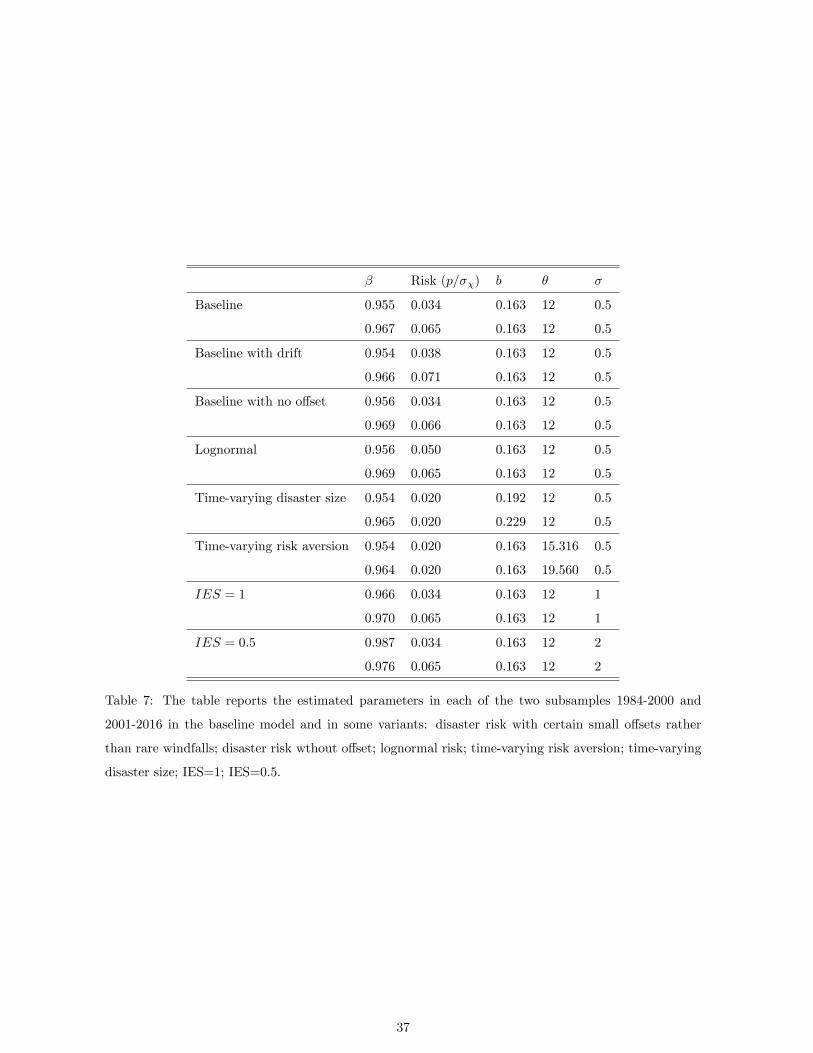
� Risk (p=��) b � �
Baseline 0.955 0.034 0.163 12 0.5
0.967 0.065 0.163 12 0.5
Baseline with drift 0.954 0.038 0.163 12 0.5
0.966 0.071 0.163 12 0.5
Baseline with no o¤set 0.956 0.034 0.163 12 0.5
0.969 0.066 0.163 12 0.5
Lognormal 0.956 0.050 0.163 12 0.5
0.969 0.065 0.163 12 0.5
Time-varying disaster size 0.954 0.020 0.192 12 0.5
0.965 0.020 0.229 12 0.5
Time-varying risk aversion 0.954 0.020 0.163 15.316 0.5
0.964 0.020 0.163 19.560 0.5
IES = 1 0.966 0.034 0.163 12 1
0.970 0.065 0.163 12 1
IES = 0:5 0.987 0.034 0.163 12 2
0.976 0.065 0.163 12 2
Table 7: The table reports the estimated parameters in each of the two subsamples 1984-2000 and
2001-2016 in the baseline model and in some variants: disaster risk with certain small o¤sets rather
than rare windfalls; disaster risk wthout o¤set; lognormal risk; time-varying risk aversion; time-varying
disaster size; IES=1; IES=0.5.
37

Risk-free rate Price-dividend Tobin�s Q
� risk others � risk others � risk others
Baseline -1.25 -1.62 -0.26 31.89 -13.34 -10.77 1.09 -0.48 0.74
Baseline with drift -1.20 -1.67 -0.26 30.03 -11.74 -10.50 1.02 -0.43 0.74
Baseline with no o¤set -1.35 -1.53 -0.26 35.92 -16.73 -11.40 1.22 -0.61 0.73
Lognormal -1.29 -1.59 -0.26 33.34 -14.57 -10.99 1.13 -0.53 0.74
Time-varying disaster size -1.08 -1.80 -0.26 25.86 -8.11 -9.97 0.89 -0.29 0.74
Time-varying risk aversion -1.07 -1.81 -0.26 25.48 -7.77 -9.93 0.87 -0.28 0.74
IES = 1 -0.43 -2.12 -0.59 9.30 0.00 -1.52 0.33 0.00 1.01
IES = 0:5 1.21 -3.11 -1.24 -39.14 28.43 18.49 -1.45 0.97 1.82
Table 8: The table reports for each variant of the baseline model, the decomposition of the risk-free
rate, the price-dividend ratio, and Tobin�s Q, into the changes driven by (i) the discount factor, (ii) the
risk parameter, (iii) all the other parameters.
in the price-dividend ratio ad in Tobin�s Q is the result of o¤setting e¤ects of the decline of � and the
increase of the risk factor. Hence, our results are insensitive to the exact way risk is modeled.
6.2 Leverage
Our model calculations assume an all-equity �nanced �rm. In reality corporations are leveraged, which
may a¤ect in particular the price-dividend ratio, which we use as an input in our estimation strategy.
In this section, we propose a simple approach to bound the e¤ect of leverage. To take this into account,
we assume a Modigliani-Miller world where corporate leverage has no e¤ect on real quantities, and
only a¤ects prices and dividends. We assume corporate debt is fully risk-free. We then adjust the
price-dividend ratio of the model given an exogenous leverage decision which we take directly from the
data.21 We then re-estimate the model and obtain the results shown in the third set of columns in tables
9 and 10.22
Qualitatively, the �ndings are quite similar to those of the model without leverage: �; � and p all
go up, and are important contributors to the observed changes in the risk-free rate, pro�tability, and
the price-dividend ratio. However, the role of risk is somewhat smaller than in our baseline version.
The logic is clear from the Gordon formula: with leverage, the change in r� required to account for the
change in valuation ratio is smaller. (Going in the other direction, however, is that in our data, aggregate
leverage declines from the �rst sample to the second one.) In particular for the spread decomposition
MPK �RF in table 10, the share of the spread due to risk is smaller (2.08 and 3.81 percentage points
21Speci�cally, we use Standard and Poors data and de�ne leverage as short-term debt plus long-term debt less cash,
divided by market value of equity.22As an alternative approach, one can adjust the r� from the model directly to account for leverage, noting that the
r� identi�ed by the model from the PD ratio is actually (1 + !)r� � !rf where ! is the observed debt-equity ratio. This
approach yields nearly identical results to the one where we adjust the PD ratio directly.
38

IES=0.5 Leverage AA rate as RF 10 year adj. for TP
1984-00 2001-16 Di¤. 1984-00 2001-16 Di¤. 1984-00 2001-16 Di¤. 1984-00 2001-16 Di¤.
� 0.987 0.976 -0.012 1.002 0.995 -0.006 0.995 0.982 -0.013 0.958 0.966 0.009
� 1.079 1.146 0.067 1.106 1.191 0.084 1.079 1.146 0.067 1.079 1.146 0.067
p 0.034 0.065 0.031 0.021 0.044 0.023 0.012 0.043 0.031 0.052 0.061 0.009
� 2.778 3.243 0.465 2.778 3.243 0.465 2.778 3.243 0.465 2.778 3.243 0.465
� 0.244 0.243 -0.000 0.224 0.214 -0.010 0.244 0.243 -0.000 0.244 0.243 -0.000
gP 1.171 1.101 -0.069 1.171 1.101 -0.069 1.171 1.101 -0.069 1.171 1.101 -0.069
gZ 1.298 1.012 -0.286 1.378 1.096 -0.282 1.298 1.012 -0.286 1.298 1.012 -0.286
gQ 1.769 1.127 -0.643 1.769 1.127 -0.643 1.769 1.127 -0.643 1.769 1.127 -0.643
N 62.344 60.838 -1.507 62.344 60.838 -1.507 62.344 60.838 -1.507 62.344 60.838 -1.507
Table 9: The table reports the estimated parameters in each of the two subsamples 1984-2000 and
2001-2016 in the baseline model, in the model with IES=0.5, in the model with �nancial leverage, and
in the model estimated with a di¤erent interest rate target (AA).
in the �rst and second sample respectively). However, the share of the increase in the spread due to risk
remains substantial. Moreover, in terms of the implied equity premium, the increase is actually similar,
because leverage now ampli�es the variation in r�:Working against us here is that we have assumed that
corporate debt pays the same return as the risk-free asset; in reality, corporate debt yields are higher
than Treasuries yields, which would reduce the adjustment to the PD ratio.
6.3 Intertemporal elasticity of substitution
We have assumed an elasticity of substitution equal to 2 in our baseline estimation. The IES also cannot
be identi�ed given that the model generates iid growth rates for all macroeconomic variables. As noted
above, the assumed value for the IES does not a¤ect estimates of �, �, r�; or the equity premium.
This can be veri�ed in tables 9 and 10 where we present parameter estimates for an elasticity equal
to 0.5. Our conclusions that risk and market power increased are hence completely una¤ected by this
assumption. However, changing the IES does a¤ect the counterfactual decompositions studied above;
for instance the e¤ect of an increase in risk on capital accumulation depends on the assumed IES.
Table 8 presents decompositions for three �nancial variables, and the appendix provides the decom-
positions of all variables. With a low IES, the e¤ect of the decline of growth in accounting for the decline
of the risk-free rate is larger. The model hence does not require an increase in � - rather � falls. The
sensitivity of the risk-free rate to uncertainty is now larger. In this sense, a lower IES hence gives a
larger role for risk. As emphasized by Bansal and Yaron (2004), higher risk and lower growth both raise
the PD ratio because of their strong e¤ect on the risk-free rate.
39

IE S= 0 .5 L e v e r a g e A A ra t e a s R F 1 0 y e a r a d j . f o r T P
1 9 8 4 - 0 0 2 0 0 1 - 1 6 D i¤ . 1 9 8 4 - 0 0 2 0 0 1 - 1 6 D i¤ . 1 9 8 4 - 0 0 2 0 0 1 - 1 6 D i¤ . 1 9 8 4 - 0 0 2 0 0 1 - 1 6 D i¤ .
A. MPK-RF spread
Total spread 11.22 15.24 4.02 11.22 15.24 4.02 9.32 13.80 4.48 12.49 14.98 2.49
- Depreciation 4.55 4.37 -0.18 4.55 4.37 -0.18 4.55 4.37 -0.18 4.55 4.37 -0.18
- Market power 3.39 5.55 2.17 4.47 6.99 2.52 3.39 5.55 2.17 3.39 5.55 2.17
- Risk premium 3.15 5.23 2.08 2.08 3.81 1.73 1.25 3.79 2.54 4.42 4.97 0.55
B. Rate of returns
Equity return 5.85 4.90 -0.96 5.77 4.84 -0.93 5.88 4.84 -1.05 5.87 4.88 -0.99
Equity premium 3.07 5.25 2.18 2.99 5.19 2.20 1.19 3.75 2.56 4.35 4.97 0.62
Risk-free rate 2.79 -0.35 -3.14 2.79 -0.35 -3.14 4.69 1.09 -3.60 1.52 -0.09 -1.61
C. Valuation ratios
Price-dividend 42.34 50.11 7.78 NA NA NA 42.34 50.11 7.78 42.34 50.11 7.78
Price-earnings 17.85 25.79 7.94 NA NA NA 17.85 25.79 7.94 17.85 25.79 7.94
Tobin�s Q 2.50 3.84 1.34 NA NA NA 2.50 3.84 1.34 2.50 3.84 1.34
D. Income shares
Share Labor 70.11 66.01 -4.10 70.11 66.01 -4.10 70.11 66.01 -4.10 70.11 66.01 -4.10
Share Capital 22.59 21.24 -1.35 20.26 17.96 -2.30 22.59 21.24 -1.35 22.59 21.24 -1.35
Share Pro�t 7.30 12.76 5.46 9.62 16.03 6.40 7.30 12.76 5.46 7.30 12.76 5.46
E. Macroeconomy
K/Y 2.13 2.28 0.15 2.13 2.28 0.15 2.13 2.28 0.15 2.13 2.28 0.15
I/Y 17.28 16.50 -0.78 17.28 16.50 -0.78 17.28 16.50 -0.78 17.28 16.50 -0.78
Detrend Y (%chg) � � -0.30 � � -1.88 � � -0.30 � � -0.30
Detrend I (%chg) � � -4.95 � � -6.52 � � -4.95 � � -4.95
Table 10: The table reports some moments of interest calculated in the baseline model, in the model
with IES=0.5, in the model with �nancial leverage, and in the model estimated with a di¤erent interest
rate target (AA), using the estimated parameter values for each of the two subsamples 1984-2000 and
2001-2016, as well as the change between samples.
40

6.4 Liquidity and term premia
As a risk-free rate proxy in the data, we use the one year Treasury rate (minus lagged core in�ation).
One concern is that our model abstracts from the liquidity premium which makes this rate especially
low. To gauge the role of the liquidity premium, we instead use as a risk-free rate proxy the rate on
AAA/AA corporate bonds, minus the SPF median CPI in�ation over the next 10 years. This is a longer
maturity rate for securities which furthermore do not possess the same unique liquidity attributes as a
US Treasury. We then repeat our estimation. The rightmost columns of tables 9 and 10 show the results.
Given the identi�cation provided by the model, changing the risk-free rate does not a¤ect �; �; or r�:
However, the di¤erent risk-free rate target will a¤ect the value of � and the amount of risk identi�ed
by the model, and their respective changes. Indeed, we see that the estimated � does not increase
across samples. The level of risk estimated is smaller, but crucially, our model still estimates that risk
increased signi�cantly between the two samples. Our conclusion about the relative importance of risk
and markups is not a¤ected by this change in target, suggesting that liquidity considerations do not
play a very large role in these trends.
A related concern is that long-term rates re�ect term premia which may be driven by an in�ation
premium, which is not present in the model. We hence consider as target for the risk-free rate the 10 year
Treasury constant maturity rate, less SPF expected in�ation, less the term premium estimate of Adrian,
Crump and Moench, which is obtained from a statistical term structure model. Because the term premia
estimate decline strongly during this period, the decline in this measure of risk-free rate is only 1.5 point
rather than over 3 points. The resulting estimates imply a smaller increase in macroeconomic risk.
Moreover, the spread MPK � RF is also increasing by a smaller amount, and the contribution of risk
premia is smaller there as well. We view these results as somewhat less plausible because the decline of
term premium implied by this model is very large - we are unaware of macroeconomic models that can
rationalize this. Also, to the extent that the decline of term premium is related to macroeconomic risk,
it may not be sound to adjust for it.
6.5 Capital mismeasurement
One natural explanation for the rising spreadMPK�RF is that K is mismeasured, and in particular is
underestimated by the BEA analysts, who traditionally focus on tangible assets. To get a sense of how
much mismeasurement of capital matters, we present a simple approach in this section. In the online
appendix, we then estimate a more detailed model of intangible accumulation. We are interested in two
questions: �rst, can a plausible amount of mismeasurement explain the rising spread? Second, is this
mismeasurement also consistent with the other observed features of the data?
In this section, we simply assume that the BEA measures only a fraction � of total investment. When
� = 1; there is no mismeasurement, corresponding to our baseline model. When � < 1 however, this
mismeasurement of investment a¤ects our target moments, and hence possibly our parameter estimates.
Denote with a superscript m the measured values of the model variables.23 Measured investment is
xm = �x; and hence along the balanced growth path km = �k: Moreover, GDP and the pro�t share are
23We do the algebra for detrended variables, but one can obviously also apply the same adjustments to the level variables.
41
now under-estimated since the unmeasured investment (1� �)x is treated as an intermediate input by
BEA accountants. As a result, measured GDP is ym = y � (1� �)x: Measured pro�ts equal measured
GDP less labor compensation, or �m = � � (1� �)x: The pro�t share is hence underestimated as
�m
ym=� � (1� �)xy � (1� �)x <
�
y:
However, dividends are correctly measured since the unmeasured investment reduces both pro�ts and
investment: d = � � x = �m � xm: Hence, the asset price is una¤ected by measurement error (even if
investors do not observe intangible investment).
It is easy to extend our formula 26:
MPK � rf = � + gQ +�� 1�
(r� + � + gQ) + r� � rf +
1� ��
d
k; (28)
and mismeasurement (� < 1) now adds an additional component to the measured spread, consistent
with basic intuition.
How important is this mismeasurement wedge? First, note that the measured ratio d=(�k) is fairly
small, around 7.5% in the second sample (and 6% in the �rst sample), according to our data moments.
Hence, with � = 0:8, or a 20 percent under-measurement, the wedge is 1.2-1.5 point, which is signi�cant.
Our focus, however, is on the increase in the spread. To explain this increase requires a rising mismea-
surement. While there is wide agreement that intangibles play a critical role in modern economies, it
is not as clear if mismeasurement has increased over the past few decades. Suppose however, that one
wanted to generate an increase the spread by 2 percentage points (or about half of the increase in the
spread observed during our sample, and about the same as what is explained by risk premia or markups
according to our baseline results), the model requires � to go for instance from 1 (perfect measurement)
to � = 0:73, a 27% underestimation of investment. This rising mismeasurement would reduce measured
GDP by 4.4% and the pro�t share by 4 percentage points. One tension, hence, is that rising intangibles
lead to a measured labor share going up rather than down, as in the data.
To evaluate more precisely how this mismeasurement a¤ects our results, we estimate three versions of
our baseline model corresponding to di¤erent assumptions about mismeasurement. In the �rst version,
mismeasurement is constant at 10% in both samples (� = 0:9). In the second version, mismeasurement
starts at 10% in the �rst subsample then rises to 20% in the second subsample. In the third version,
mismeasurement starts at 10% then rises to 30%. These numbers are largely illustrative; note however
that the share in capital of measured �intangibles�, that is intellectual property products, is about 6%
recently. We are hence assuming that the unmeasured stock of intangible capital is signi�cantly larger
than the current measured stock, and has been rising importantly over the past 15 years.
Table 11 reports the parameter estimates and table 12 reports the implied moments corresponding to
di¤erent scenarios. There are a few interesting results. First, all parameters are completely una¤ected,
except for � and �: In particular, the increase in � and in risk are not a¤ected by these assumptions.
Second, when mismeasurement is constant at 10%, the model has similar implications to our baseline
model (the level of � is higher and the level of � lower, but the changes between two subsamples are
nearly identical). Third, the estimated increase in markup is smaller when there is an increase in
mismeasurement. For instance, with a mismeasurement rising to 30% of capital, the markup rises by
42
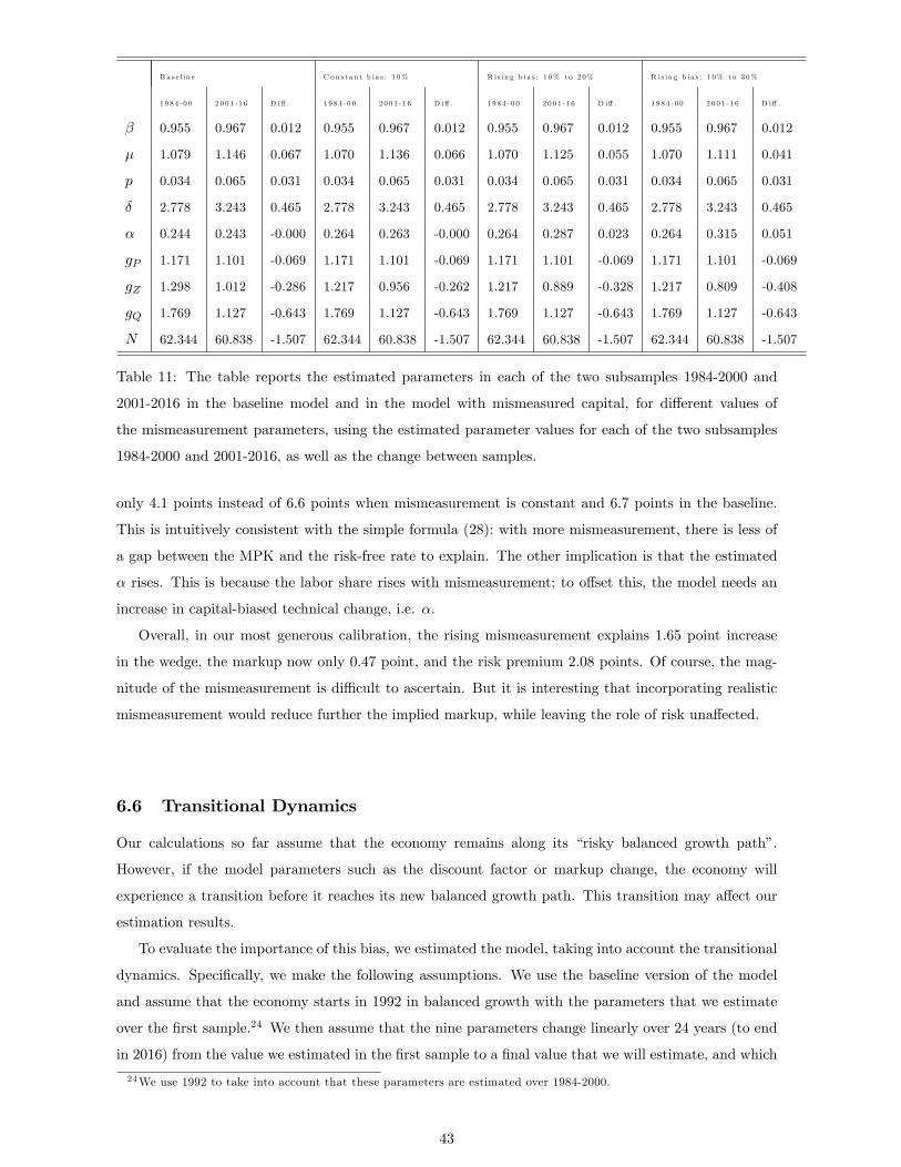
B a s e l in e C o n s t a n t b ia s : 1 0% R is in g b ia s : 1 0% to 2 0% R is in g b ia s : 1 0% to 3 0%
1 9 8 4 - 0 0 2 0 0 1 - 1 6 D i¤ . 1 9 8 4 - 0 0 2 0 0 1 - 1 6 D i¤ . 1 9 8 4 - 0 0 2 0 0 1 - 1 6 D i¤ . 1 9 8 4 - 0 0 2 0 0 1 - 1 6 D i¤ .
� 0.955 0.967 0.012 0.955 0.967 0.012 0.955 0.967 0.012 0.955 0.967 0.012
� 1.079 1.146 0.067 1.070 1.136 0.066 1.070 1.125 0.055 1.070 1.111 0.041
p 0.034 0.065 0.031 0.034 0.065 0.031 0.034 0.065 0.031 0.034 0.065 0.031
� 2.778 3.243 0.465 2.778 3.243 0.465 2.778 3.243 0.465 2.778 3.243 0.465
� 0.244 0.243 -0.000 0.264 0.263 -0.000 0.264 0.287 0.023 0.264 0.315 0.051
gP 1.171 1.101 -0.069 1.171 1.101 -0.069 1.171 1.101 -0.069 1.171 1.101 -0.069
gZ 1.298 1.012 -0.286 1.217 0.956 -0.262 1.217 0.889 -0.328 1.217 0.809 -0.408
gQ 1.769 1.127 -0.643 1.769 1.127 -0.643 1.769 1.127 -0.643 1.769 1.127 -0.643
N 62.344 60.838 -1.507 62.344 60.838 -1.507 62.344 60.838 -1.507 62.344 60.838 -1.507
Table 11: The table reports the estimated parameters in each of the two subsamples 1984-2000 and
2001-2016 in the baseline model and in the model with mismeasured capital, for di¤erent values of
the mismeasurement parameters, using the estimated parameter values for each of the two subsamples
1984-2000 and 2001-2016, as well as the change between samples.
only 4.1 points instead of 6.6 points when mismeasurement is constant and 6.7 points in the baseline.
This is intuitively consistent with the simple formula (28): with more mismeasurement, there is less of
a gap between the MPK and the risk-free rate to explain. The other implication is that the estimated
� rises. This is because the labor share rises with mismeasurement; to o¤set this, the model needs an
increase in capital-biased technical change, i.e. �:
Overall, in our most generous calibration, the rising mismeasurement explains 1.65 point increase
in the wedge, the markup now only 0.47 point, and the risk premium 2.08 points. Of course, the mag-
nitude of the mismeasurement is di¢ cult to ascertain. But it is interesting that incorporating realistic
mismeasurement would reduce further the implied markup, while leaving the role of risk una¤ected.
6.6 Transitional Dynamics
Our calculations so far assume that the economy remains along its �risky balanced growth path�.
However, if the model parameters such as the discount factor or markup change, the economy will
experience a transition before it reaches its new balanced growth path. This transition may a¤ect our
estimation results.
To evaluate the importance of this bias, we estimated the model, taking into account the transitional
dynamics. Speci�cally, we make the following assumptions. We use the baseline version of the model
and assume that the economy starts in 1992 in balanced growth with the parameters that we estimate
over the �rst sample.24 We then assume that the nine parameters change linearly over 24 years (to end
in 2016) from the value we estimated in the �rst sample to a �nal value that we will estimate, and which
24We use 1992 to take into account that these parameters are estimated over 1984-2000.
43

B a s e l in e C o n s t a n t b ia s : 1 0% R is in g b ia s : 1 0% to 2 0% R is in g b ia s : 1 0% to 3 0%
1 9 8 4 - 0 0 2 0 0 1 - 1 6 D i¤ . 1 9 8 4 - 0 0 2 0 0 1 - 1 6 D i¤ . 1 9 8 4 - 0 0 2 0 0 1 - 1 6 D i¤ . 1 9 8 4 - 0 0 2 0 0 1 - 1 6 D i¤ .
A. MPK-RF spread
Total spread 11.22 15.24 4.02 11.22 15.24 4.02 11.22 15.24 4.02 11.22 15.24 4.02
- Depreciation 4.55 4.37 -0.18 4.55 4.37 -0.18 4.55 4.37 -0.18 4.55 4.37 -0.18
- Market power 3.39 5.55 2.17 2.80 4.79 1.99 2.80 4.03 1.23 2.80 3.27 0.47
- Risk premium 3.15 5.23 2.08 3.15 5.23 2.08 3.15 5.23 2.08 3.15 5.23 2.08
B. Rate of returns
Equity return 5.85 4.90 -0.96 5.85 4.90 -0.96 5.85 4.90 -0.96 5.85 4.90 -0.96
Equity premium 3.07 5.25 2.18 3.07 5.25 2.18 3.07 5.25 2.18 3.07 5.25 2.18
Risk-free rate 2.79 -0.35 -3.14 2.79 -0.35 -3.14 2.79 -0.35 -3.14 2.79 -0.35 -3.14
C. Valuation ratios
Price-dividend 42.34 50.11 7.78 42.34 50.11 7.78 42.34 50.11 7.78 42.34 50.11 7.78
Price-earnings 17.85 25.79 7.94 17.85 25.79 7.94 17.85 25.79 7.94 17.85 25.79 7.94
Tobin�s Q 2.50 3.84 1.34 2.50 3.84 1.34 2.50 3.84 1.34 2.50 3.84 1.34
D. Income shares
Share Labor 70.11 66.01 -4.10 68.79 64.82 -3.97 68.79 63.39 -5.40 68.79 61.65 -7.14
Share Capital 22.59 21.24 -1.35 24.63 23.17 -1.46 24.63 25.49 0.87 24.63 28.33 3.71
Share Pro�t 7.30 12.76 5.46 6.58 12.01 5.43 6.58 11.11 4.53 6.58 10.02 3.44
E. Macroeconomy
K/Y 2.13 2.28 0.15 2.13 2.28 0.15 2.13 2.28 0.15 2.13 2.28 0.15
I/Y 17.28 16.50 -0.78 17.28 16.50 -0.78 17.28 16.50 -0.78 17.28 16.50 -0.78
Detrend Y (% chg) � � -0.30 � � -0.04 � � 7.88 � � 18.53
Detrend I (% chg) � � -4.95 � � -4.60 � � 12.87 � � 34.08
Table 12: The table reports some moments of interest calculated in the baseline model and in the model
with mismeasured capital, for di¤erent values of the mismeasurement parameters, using the estimated
parameter values for each of the two subsamples 1984-2000 and 2001-2016, as well as the change between
samples.
44

may not be our estimate for the second sample.
We then calculate the transitional dynamics for this economy using a standard shooting method. A
key issue is agents�expectations. With perfect foresight, the model cannot �t the data, because agents
see the lower interest rates coming, which leads to a boom in the price-dividend ratio. (Furthermore, the
long-term interest rate would fall signi�cantly more than the short rate, unlike what we see in the data.)
We hence assume myopic expectations: each period, agents observe the new values of the parameters,
and they assume (incorrectly, at least for the �rst 24 years) that these parameters will remain constant
forever.25
We then numerically �nd the �nal parameters such that, when calculating the transition, this pro-
cedure yields an average time series for our targets (over the period 2001-2016) that matches what we
measured in the data. We are able to �nd a close, though not perfect, match. Figure 13 presents the
path obtained for parameter values and �gure 14 the path for the moments targeted (we abstract here
from parameters that map directly into moments). Table 13 presents the numerical counterpart to these
graphs.
As can be seen in �gure 14, the model moments, averaged over periods 10-26 (i.e. 2001-2016), match
reasonably well the target moments for the second sample (in red). The more surprising result is in �gure
13, where we see that the parameter values estimated in this way are quite similar to these obtained in
the simple baseline model, which assumes balanced growth. To see this, note that the blue line, averaged
over periods 10-26, is economically quite similar to the red line (results from the baseline model). The
one exception is �; which now falls slightly instead of rising. Table 13 shows the same result: comparing
the third and fourth columns, the estimated parameters are quite similar, except for �: We view this
results as suggesting that, at least in the myopic case, perhaps not much is lost by focusing on the risky
balanced growth path. This conclusion might not hold true for all models however; in particular with
intangibles if there is signi�cant accumulation during the transition.
7 Other evidence on market power, risk premia and intangibles
Our empirical results show that rising risk premia and rising market power appear to be two of the
signi�cant drivers of some of the macro-�nance trends we focus on, and intangibles have a potential
contribution as well. In this section we step outside of the model and present some simpler and inde-
pendent evidence for these two phenomena. We also discuss some related estimates presented by other
researchers, which tend to support our conclusions.
25Agents consequently make investment choices that would, eventually, lead to converge to a new steady-state corre-
sponding to today�s parameter values. However, the next period, new parameter values (unexpectedly) arrive, leading
to new choices and a revised transition path. This process continues until the parameters are indeed constant, and the
economy then converges to its �nal steady-state.
45
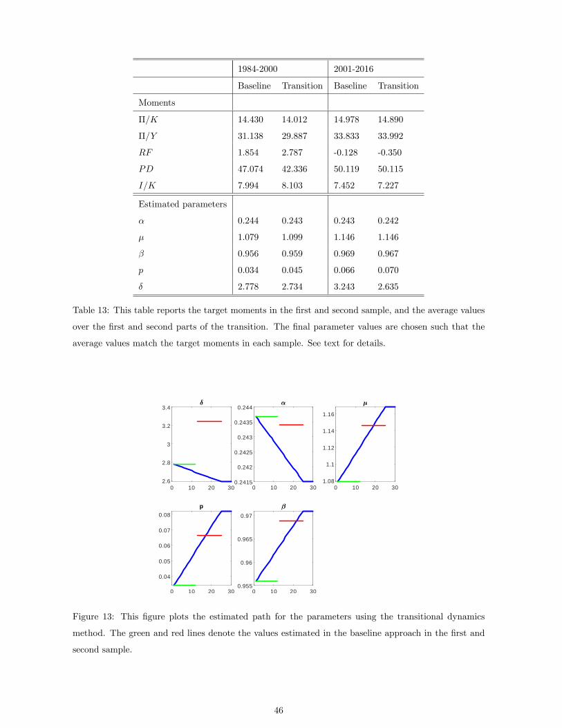
1984-2000 2001-2016
Baseline Transition Baseline Transition
Moments
�=K 14.430 14.012 14.978 14.890
�=Y 31.138 29.887 33.833 33.992
RF 1.854 2.787 -0.128 -0.350
PD 47.074 42.336 50.119 50.115
I=K 7.994 8.103 7.452 7.227
Estimated parameters
� 0.244 0.243 0.243 0.242
� 1.079 1.099 1.146 1.146
� 0.956 0.959 0.969 0.967
p 0.034 0.045 0.066 0.070
� 2.778 2.734 3.243 2.635
Table 13: This table reports the target moments in the �rst and second sample, and the average values
over the �rst and second parts of the transition. The �nal parameter values are chosen such that the
average values match the target moments in each sample. See text for details.
0 10 20 302.6
2.8
3
3.2
3.4
0 10 20 300.2415
0.242
0.2425
0.243
0.2435
0.244
0 10 20 301.08
1.1
1.12
1.14
1.16
0 10 20 30
0.04
0.05
0.06
0.07
0.08p
0 10 20 300.955
0.96
0.965
0.97
Figure 13: This �gure plots the estimated path for the parameters using the transitional dynamics
method. The green and red lines denote the values estimated in the baseline approach in the �rst and
second sample.
46
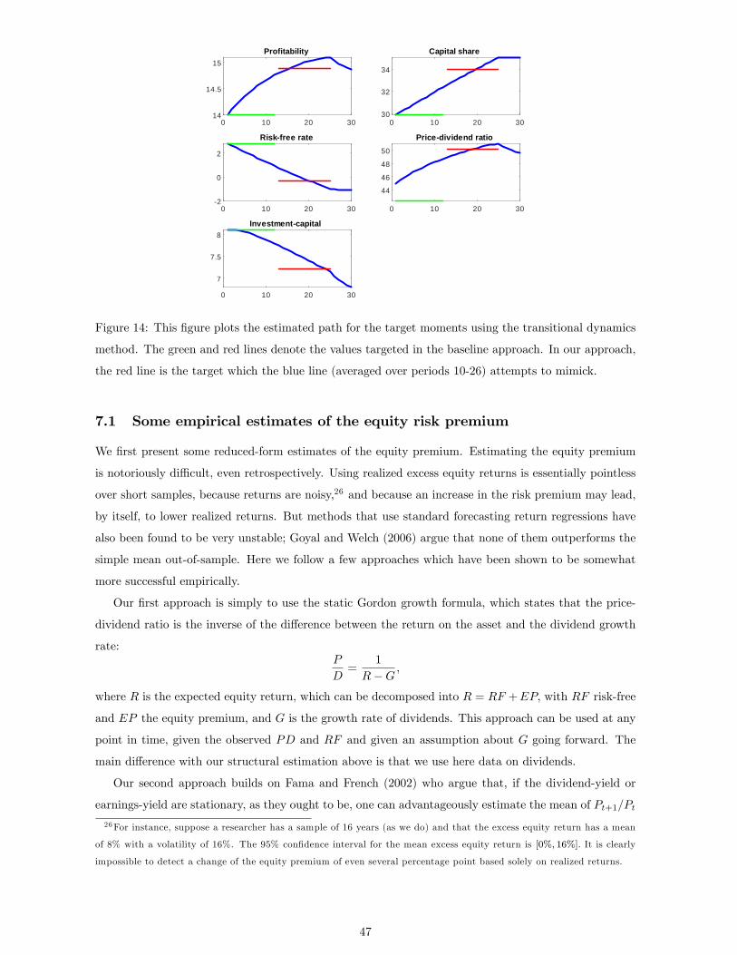
0 10 20 3014
14.5
15Profitability
0 10 20 3030
32
34
Capital share
0 10 20 302
0
2
Riskfree rate
0 10 20 30
44
46
48
50
Pricedividend ratio
0 10 20 30
7
7.5
8Investmentcapital
Figure 14: This �gure plots the estimated path for the target moments using the transitional dynamics
method. The green and red lines denote the values targeted in the baseline approach. In our approach,
the red line is the target which the blue line (averaged over periods 10-26) attempts to mimick.
7.1 Some empirical estimates of the equity risk premium
We �rst present some reduced-form estimates of the equity premium. Estimating the equity premium
is notoriously di¢ cult, even retrospectively. Using realized excess equity returns is essentially pointless
over short samples, because returns are noisy,26 and because an increase in the risk premium may lead,
by itself, to lower realized returns. But methods that use standard forecasting return regressions have
also been found to be very unstable; Goyal and Welch (2006) argue that none of them outperforms the
simple mean out-of-sample. Here we follow a few approaches which have been shown to be somewhat
more successful empirically.
Our �rst approach is simply to use the static Gordon growth formula, which states that the price-
dividend ratio is the inverse of the di¤erence between the return on the asset and the dividend growth
rate:P
D=
1
R�G;
where R is the expected equity return, which can be decomposed into R = RF +EP; with RF risk-free
and EP the equity premium, and G is the growth rate of dividends. This approach can be used at any
point in time, given the observed PD and RF and given an assumption about G going forward. The
main di¤erence with our structural estimation above is that we use here data on dividends.
Our second approach builds on Fama and French (2002) who argue that, if the dividend-yield or
earnings-yield are stationary, as they ought to be, one can advantageously estimate the mean of Pt+1=Pt26For instance, suppose a researcher has a sample of 16 years (as we do) and that the excess equity return has a mean
of 8% with a volatility of 16%. The 95% con�dence interval for the mean excess equity return is [0%; 16%]: It is clearly
impossible to detect a change of the equity premium of even several percentage point based solely on realized returns.
47

Arithmetic average Geometric average
1984�00 2001-16 Change 1984��00 2001-�16 Change
Real dividend growth 2.03 4.7 2.67 2.04 8.21 6.17
Real earnings growth 6.22 16.97 10.75 10.25 12.06 1.81
Return on book equity 10.94 10 -.94 10.7 9.4 -1.3
D/P 2.78 1.92 -.86 � � �
D/E .49 .47 -.02 � � �
E/P 5.74 4.69 -1.05 � � �
ERP Gordon .87 5.56 4.69 1.91 9.16 7.25
ERP Fama-French Earnings 2.43 4.78 2.35 4.61 8.66 4.05
ERP Campbell-Thompson 1.47 4.11 2.64 1.84 3.65 1.81
ERP Gordon - w. variance adj � � � 2.43 8.26 5.83
ERP Fama-French Earnings - w. var. adj. � � � 4.81 10.3 5.49
ERP Campbell-Thompson - w. var. adj. � � � 2.31 5.56 3.25
Table 14: The table reports estimates of the equity premium for the samples 1984-2000 and 2001-2016.
See text for details.
by Dt+1=Dt or Et+1=Et (which are less volatile). As a result, they suggest estimating
ERP = E
�Dt+1
Pt
�+ E
�Dt+1
Dt
�� E(RF );
which amounts to the Gordon growth formula, or replacing dividend growth with earnings growth,
ERP = E
�Dt+1
Pt
�+ E
�Et+1Et
�� E(RF ):
This approach is best thought as applying to a long-sample average.
Our third approach follows Campbell and Thompson (2008) who show how combining the current
dividend yield and the return on book equity can be used to create a real-time estimate of the equity
premium:
ERP =D
E
E
P+
�1� D
E
�ROE;
and where they suggest smoothing the payout ratio D=E, earnings-price ratio E=P; and the return on
book equity ROE to reduce the e¤ect of in�uential but transitory observations.
These formulas can be applied either using arithmetic averages or using geometric averages. We
report both below in table 14, though we like Campbell and Thompson�s recommendation to use the
geometric averages. We then incorporate an adjustment of 1=2 the variance of stock returns to produce
an estimate of arithmetic equity premium.
The key observation from table 14 is that, while the estimates of the equity premium are clearly
di¤erent across models and methods, most calculations suggest that the ERP increased from the �rst
sample to the second sample. Speci�cally, all nine estimates in bold are positive, ranging from 1.8%
48
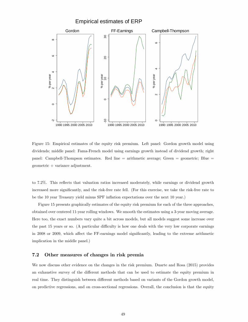
20
24
68
% p
er y
ear
1990 1995 2000 2005 2010
Gordon
10
010
2030
% p
er y
ear
1990 1995 2000 2005 2010
FFEarnings
02
46
% p
er y
ear
1990 1995 2000 2005 2010
CampbellThompson
Empirical estimates of ERP
Figure 15: Empirical estimates of the equity risk premium. Left panel: Gordon growth model using
dividends; middle panel: Fama-French model using earnings growth instead of dividend growth; right
panel: Campbell-Thompson estimates. Red line = arithmetic average; Green = geometric; Blue =
geometric + variance adjustment.
to 7.2%. This re�ects that valuation ratios increased moderately, while earnings or dividend growth
increased more signi�cantly, and the risk-free rate fell. (For this exercise, we take the risk-free rate to
be the 10 year Treasury yield minus SPF in�ation expectations over the next 10 year.)
Figure 15 presents graphically estimates of the equity risk premium for each of the three approaches,
obtained over centered 11-year rolling windows. We smooth the estimates using a 3-year moving average.
Here too, the exact numbers vary quite a bit across models, but all models suggest some increase over
the past 15 years or so. (A particular di¢ culty is how one deals with the very low corporate earnings
in 2008 or 2009, which a¤ect the FF-earnings model signi�cantly, leading to the extreme arithmetic
implication in the middle panel.)
7.2 Other measures of changes in risk premia
We now discuss other evidence on the changes in the risk premium. Duarte and Rosa (2015) provides
an exhaustive survey of the di¤erent methods that can be used to estimate the equity premium in
real time. They distinguish between di¤erent methods based on variants of the Gordon growth model,
on predictive regressions, and on cross-sectional regressions. Overall, the conclusion is that the equity
49
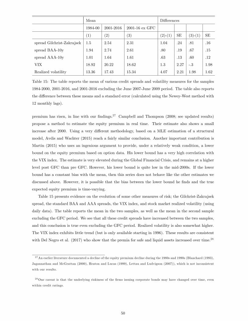
Mean Di¤erences
1984-00 2001-2016 2001-16 ex GFC
(1) (2) (3) (2)-(1) SE (3)-(1) SE
spread Gilchrist-Zakrajsek 1.5 2.54 2.31 1.04 .24 .81 .16
spread BAA-10y 1.94 2.74 2.61 .80 .19 .67 .15
spread AAA-10y 1.01 1.64 1.61 .63 .13 .60 .12
VIX 18.92 20.22 18.62 1.3 2.27 -.3 1.98
Realized volatility 13.36 17.43 15.34 4.07 2.21 1.98 1.62
Table 15: The table reports the mean of various credit spreads and volatility measures for the samples
1984-2000, 2001-2016, and 2001-2016 excluding the June 2007-June 2009 period. The table also reports
the di¤erence between these means and a standard error (calculated using the Newey-West method with
12 monthly lags).
premium has risen, in line with our �ndings.27 Campbell and Thompson (2008; see updated results)
propose a method to estimate the equity premium in real time. Their estimate also shows a small
increase after 2000. Using a very di¤erent methodology, based on a MLE estimation of a structural
model, Avdis and Wachter (2015) reach a fairly similar conclusion. Another important contribution is
Martin (2015) who uses an ingenious argument to provide, under a relatively weak condition, a lower
bound on the equity premium based on option data. His lower bound has a very high correlation with
the VIX index. The estimate is very elevated during the Global Financial Crisis, and remains at a higher
level post GFC than pre GFC. However, his lower bound is quite low in the mid-2000s. If the lower
bound has a constant bias with the mean, then this series does not behave like the other estimates we
discussed above. However, it is possible that the bias between the lower bound he �nds and the true
expected equity premium is time-varying.
Table 15 presents evidence on the evolution of some other measures of risk; the Gilchrist-Zakrajsek
spread, the standard BAA and AAA spreads, the VIX index, and stock market realized volatility (using
daily data). The table reports the mean in the two samples, as well as the mean in the second sample
excluding the GFC period. We see that all these credit spreads have increased between the two samples,
and this conclusion is true even excluding the GFC period. Realized volatility is also somewhat higher.
The VIX index exhibits little trend (but is only available starting in 1996). These results are consistent
with Del Negro et al. (2017) who show that the premia for safe and liquid assets increased over time.28
27An earlier literature documented a decline of the equity premium decline during the 1980s and 1990s (Blanchard (1993),
Jagannathan and McGrattan (2000), Heaton and Lucas (1999), Lettau and Ludvigson (2007)), which is not inconsistent
with our results.
28One caveat is that the underlying riskiness of the �rms issuing corporate bonds may have changed over time, even
within credit ratings.
50

7.3 Independent evidence on risking markups
A number of recent contributions, using di¤erent methods, have found that average markups have been
increasing. For example, Barkai (2016) uses aggregate data and implements a user cost approach a la
Hall-Jorgenson (1967) to decompose the non-labor share into a true capital share and a pro�t share.
The true capital share is computed by multiplying the capital output ratio by the user cost of capital.
The pro�t share is a residual. The aggregate markup can be directly inferred from the pro�t share.
Because his measure of user cost does not incorporate a meaningful risk premium, Barkai �nds that
the evolutions of the user cost track those of the interest rate, and so that the user cost has declined
substantially over the period 1984-2014. This implies a large decrease in the capital share, a large
increase in the pro�t share, and a large increase in the aggregate markup of about 20% roughly in line
with our macro estimation.
De Loecker and Eeckhout (2016) use �rm-level data and estimate �rm-level markups using a produc-
tion function approach which recovers markups as the ratio of the elasticity of production to a �exible
input the the share of that input in revenues, where the former is computed by estimating the production
function. The aggregate markup computed as a harmonic sales-weighted average of �rm-level markups
increases by about 25%. Traina (2018) criticizes the measure of costs used by De Loecker and Eeck-
hout (2016). Using a broader measure, he �nds that the increase in average markups is much smaller.
Gutierrez and Philippon (2016) also use �rm-level data but they estimate �rm-level markups using a
user cost approach allowing for sizeable and variable risk premia. They also �nd a sizeable increase in
aggregate markups of about 10% over the period 1984-2014, somewhat above our baseline results.
7.4 Rising Intangible Capital
There is a growing literature that recognizes the importance of intangible capital in the US economy.
Corrado et al. (2005, 2009) and Nakamura (2010) present estimates of the size of intangible capital.
Bhandari and McGrattan (2017) also contribute to this measurement. Koh, Santaeullia-Llopis and
Zheng (2015) argue that rising intangibles help explain the evolution of the labor share. Crouzet and
Eberly (2018) argue that growing intangibles help explain both the rising market power and lower capital
investment. Caggese ad Perez (2017) show how growing intangibles may help account for some of the
same macro trends that we focus on in this paper.
8 Conclusion
We provide a simple accounting framework that allows decomposing the changes observed over the
past 30 years in some key macro-�nance trends into �semi-structural� parameters using a fairly clear
identi�cation. We say �semi-structural�because, allowing these parameters to vary over time �exibly
suggests they are not microfounded and invariant to policy. Yet we �nd the results useful because deeper
explanations have to be consistent with the changes of parameters implied by our approach.
We �nd that about half of the increase in the spread between the return on private capital and the
risk-free rate is due to rising market power, and half due to rising risk. Technical change plays little
51
role. Higher savings supply and higher risk are the prime proximate contributors to the decline of the
risk-free rate. Rising market power help explain the evolution of the capital share, pro�tability, and
capital accumulation, but its contribution is substantially overstated if the model is estimated using a
macro approach that abstracts from risk. Finally, taking into account intangibles reduces further the
estimated increase in the market power.
One limitation of our approach is that we treat the parameter changes as independent causal factors,
but they might actually be driven by common causes; for instance, higher market power might reduce
innovation and hence productivity growth, but we treat these as independent. Our analysis also does
not incorporate some factors which could help explain the evolution of some of the big ratios that we
study. In particular, we abstract from taxes and from agency issues (e.g. external �nance or corporate
governance frictions) or market incompleteness, that could also give rise to wedges that might vary over
time. Our study of transitional dynamics is only scratching at the vast possibilities. Finally, it would
be interesting to study these issues taking into account the speci�c open economy considerations or at
least to study these same facts for a variety of countries.
52
9 References
Aaronson Dan, Luojia Hu, Arian Seifoddini, and Dan Sullivan (2014). �Declining Labor Force Par-
ticipation and Its Implications for Unemployment and Employment Growth�, Economic Perspectives,
Federal Reserve Bank of Chicago, Vol. 38, 4th, 2014.
Acemoglu, Daron and Pascual Restrepo, �The race between man and machine,� NBER Working
Papers 22252 May 2016.
Andrews, Isaiah, Matthew Gentzknow and Jesse Shapiro, 2017. �Measuring the Sensitivity of Para-
meter Estimates to Estimation Moments�, Quarterly Journal of Economics. 132(4). November 2017.
Autor, David, David Dorn, Lawrence F Katz, Christina Patterson, and John Van Reenen. 2017.
�The Fall of the Labor Share and the Rise of Superstar Firms.�National Bureau of Economic Research
working paper.
Avdis Efstathios, and Jessica Wachter, . �Maximum likelihood estimation of the equity premium�,
Journal of Financial Economics 125 (3): 589-609.
Bhandari, Anmol, and Ellen R McGrattan. 2018. �Sweat Equity in US Private Business.�National
Bureau of Economic Research working paper.
Barkai, Simcha, 2016. �Declining Labor and Capital Shares�, Working paper, London Business
School.
Barro, Robert, Jesús Fernández-Villaverde, Oren Levintal, Andrew Mollerus, 2016. �Safe assets�,
NBER Working Paper No. 20652.
Barro, Robert, 2006. �Rare disasters and asset markets in the twentieth century�, Quarterly Journal
of Economics 121(3):823�866.
Campbell, John, �Estimating the Equity Premium,�Canadian Journal of Economics, February 2008,
41 (1), 1�21.
Campbell, Je¤rey, Jonas Fisher, Alejandro Justiniano, and Leo Melosi, 2017. �Forward Guidance and
Macroeconomic Outcomes Since the Financial Crisis. Chapter in NBER book NBER Macroeconomics
Annual 2016, Volume 31 (2017), Martin Eichenbaum and Jonathan A. Parker, editors (p. 283 - 357)
Caballero, Ricardo J., and Emmanuel Farhi, 2018. �The Safety Trap,�Review of Economic Studies,
2018, 85 (1).
Caballero, Ricardo J., Emmanuel Farhi and Pierre-Olivier Gourinchas, 2008. �An Equilibrium Model
of �Global Imbalances�and Low Interest Rates,�American Economic Review, March 2008, 98 (1), 358�
93.
Caballero, Ricardo J., Emmanuel Farhi and Pierre-Olivier Gourinchas, 2017. "Rents, Technical
Change, and Risk Premia Accounting for Secular Trends in Interest Rates, Returns on Capital, Earning
Yields, and Factor Shares," American Economic Review, American Economic Association, vol. 107(5),
pages 614-620, May.
Carvalho, Carlos, Andrea Ferrero, Fernanda Nechio, 2016. �Demographics and real interest rates:
Inspecting the mechanism�, European Economic Review, Volume 88, September 2016, Pages 208-226.
Corrado, Carol, Charles Hulten, and Daniel Sichel. 2009. �Intangible capital and US economic
growth.�Review of income and wealth, 55(3): 661�685.
53

Corrado, Carol, Charles Hulten, and Daniel Sichel. 2005. �Measuring capital and technology: an
expanded framework.�In Measuring capital in the new economy. 11�46. University of Chicago Press.
Crouzet, Nicolas and Janice Eberly, 2018. �Understanding Weak Capital Investment: the Role of
Market Concentration and Intangibles�, Jackson Hole Economic Policy Symposium,. Federal Reserve
Bank of Kansas City.
De Loecker, Jan and Jan Eeckhout, 2017. �The Rise of Market Power and the Macroeconomic
Implications�, NBER Working paper 23687.
Del Negro, Marco, Domenico Giannone, Marc Giannoni, and Andrea tambalotti, 2017. �Safety,
Liquidity, and the Natural Rate of Interest�, Brookings Papers on Economic Activity (Spring 2017), pp.
235-294.
Duarte, Fernando, and Carlo Rosa, 2015. �The Equity Risk Premium: A Review of Models�, Federal
Reserve Bank of New York Sta¤ Report 714.
Eberly.Janice Investment and Alexander Lewis. �Investement hollowing out.� IMF Economic Re-
view, 2017.
Eggertsson, Gauti, Jacob A. Robbins, Ella Getz Wold Kaldor and Piketty�s Facts: The Rise of
Monopoly Power in the United States, NBER Working paper 24287.
Eggertsson, Gauti, Neil R. Mehrotra, Jacob A. Robbin. �A Model of Secular Stagnation: Theory
and Quantitative Evaluation�, NBER Working paper 23093.
Elsby, M. W., B. Hobjin, and A. Sahin (2013): �The decline of the US labor share,� Brookings
Papers on Economic Activity, 2013(2), 1�63.
Fama, Eugene F. and Kenneth R. French, 2002. �The Equity Premium�, Journal of Finance,
57(2):637-659.
Fernald, John, 2015. �Productivity and Potential Output Before, During, and After the Great
Recession�, NBER Working Paper No. 20248 and NBER Macroeconomics Annual 2014, Volume 29,
Parker and Woodford. 2015.
Fisher, Jonas, 2015. �On the Structural Interpretation of the Smets�Wouters "Risk Premium"
Shock�, Journal of Money, Credit and Banking, Volume 47, Issue 2-3, March-April 2015, pp. 511-516.
Gabaix, Xavier, 2011. �Disasterization: A Simple Way to Fix the Asset Pricing Properties of
Macroeconomic Models�, American Economic Review, 101(3): pp 406-409.
Gabaix, Xavier, 2012. �Variable Rare Disasters: An Exactly Solved Framework for Ten Puzzles in
Macro-Finance,�Quarterly Journal of Economics, May, 645-700.
Gagnon, Etienne, Benjamin Johannsen and David López-Salido, 2016. �Understanding the New
Normal: The Role of Demographics,� Finance and Economics Discussion Series 2016-080, Board of
Governors of the Federal Reserve System.
Gomme, Paul, B. Ravikumar, and Peter Rupert, �The Return to Capital and the Business Cycle,�
Review of Economic Dynamics, April 2011, 14 (2), 262�278.
Gourio, François, 2012. �Disaster Risk and Business Cycles,�American Economic Review, 102(6):2734�
66.
Gourio, François, 2013: �Credit Risk and Disaster Risk,�American Economic Journal: Macroeco-
54
nomics, 5(3), 1�34.
Gourio, François, Anil Kashyap, and Jae Sim, 2018. �The Tradeo¤s in Leaning Against the Wind�,
IMF Economic Review.
Gourio, François, 2018: �A note on decomposition for nonlinear models,�Mimeo, Federal Reserve
Bank of Chicago.
Goyal, Amit, and Ivo Welch. �A Comprehensive Look at the Empirical Performance of Equity
Premium Prediction�. Review of Financial Studies 21(4) 1455-1508.
Gutierrez, German, and Thomas Philippon. 2017. �Investmentless Growth: An Empirical Investi-
gation.�Brookings Papers on Economic Activity, 2017(2): 89�190
Gutierrez, German, and Thomas Philippon. 2018. �Declining Competition and Investment in the
US.�National Bureau of Economic Research working paper
Hall, Robert, 2017. �The Role of the Growth of Risk-Averse Wealth in the Decline of the Safe Real
Interest Rate�, NBER working paper 22196.
Hall, Robert, 2018. �New Evidence on the Markup of Prices over Marginal Costs and the Role of
Mega-Firms in the US Economy�, Mimeo, Stanford University.
Hamilton, James D., Ethan S. Harris, Jan Hatzius and Kenneth D. West, 2015. �The Equilibrium
Real Funds Rate: Past, Present and Future, prepared for the US Monetary Policy forum.
Isore, Marlene, and Urszula Szczerbowicz, 2018. �Disaster Risk and Preference Shifts in a New
Keynesian Model�, Journal of Economics Dynamics and Control.
Karabarbounis, Loukas and Brent Neiman, 2013. �The Global Decline of the Labor Share,�The
Quarterly Journal of Economics, 129(1):61-103.
Karabarbounis, Loukas and Brent Neiman, 2018. �Accounting for Factorless Income,�NBERMacro-
economics Annual, forthcoming.
Kehrig, Matthias, and Nicolas Vincent, 2017.�Growing productivity without growing wages: The
micro-level anatomy of the aggregate labor share decline�, Working paper, Duke.
Kilic, Mete and Jessica Wachter, 2018. �Risk, Unemployment, and the Stock Market: A Rare-Event-
Based Explanation of Labor MarketVolatility�, Forthcoming, Review of Financial Studies.
Koh, Dongya, Raul Santaeullia-Llopis, and Yu Zheng, �Labor Share Decline and Intellectual Property
Products Capital,�Working Papers 927, BGSE September 2016
Kozlowski, Veldkamp and Venky Venkateswaran, �The Tail That Wags the Economy�, Working
paper, NYU.
Kozlowski, Veldkamp and Venky Venkateswaran, �The Tail That Wags the Risk Free Rate�, NBER
Macroeconomics Annual.
Martin, Ian, 2013. �Consumption-Based Asset Pricing with Higher Cumulants�, Review of Economic
Studies, 80(2):745-773.
Martin, Ian, 2017. �What is the Expected Return on the Market?�, The Quarterly Journal of
Economics, 132(1):367�433.
Marx, Magalie, Benoit Mojon and Francois Velde, 2017. �Why Have Interest Rates Fallen Far Below
the Return on Capital�, Working Paper, Federal Reserve Bank of Chicago.
55
McGrattan, Ellen R. and Edward C. Prescott, 2010, �Unmeasured Investment and the Puzzling U.S.
Boom in the 1990s�American Economic Journal: Macroeconomics, 2(4): 88�123.
Mulligan Casey, 2004: �Capital, Interest and Aggregate Intertemporal Substitution�, Working Paper,
University of Chicago.
Nakamura, Leonard I. 2010. �Intangible assets and national income accounting.�Review of Income
and Wealth, 56: S135�S155.
Rachel, Lukasz and Thomas Smith, �Are Low Real Interest Rates Here to Stay?�, International
Journal of Central Banking, 2017.
Rietz, Thomas, 1988. �The equity premium: a solution�, Journal of Monetary Economics 22(1):117�
131.
Rognlie, Matthew, 2015. �Deciphering the Fall and Rise in the Net Capital Share: Accumulation or
Scarcity?�, Brookings Papers on Economic Activity (Spring 2015), pp. 1-54
Traina, James, 2018. �Is Aggregate Market Power Increasing? Production Trends Using Financial
Statements�, Working Paper, U of Chicago.
Wachter, Jessica, 2013. �Can time-varying risk of rare disasters explain aggregate stock market
volatility?�Journal of Finance 68:987-1035, June 2013
56

10 Appendix
10.1 Data appendix
The time series that we use for our baseline estimation are constructed as follows. Our data and
programs are available online. We give Haver mnemonics. In many cases we have considered alternative
series. However, because we focus on the medium-run trends, di¤erences in cyclical behavior are muted.
- Real risk-free interest rate: in our baseline, we use the one-year constant Treasury maturity less
current in�ation (fcm1@usecon minus ypcuslfe@usecon), though results are nearly identical if other
proxies for in�ation are used, such as ex-post realized total or core in�ation or the median 1-year ahead
SPF expected in�ation (since we focus on long-term averages, these measures are nearly identical). In
the extension, we use also the AAA/AA FTSE index for corporate bond yields minus the median 10 year
ahead CPI expected in�ation (syct5a@usecon - asacx10@surveys), and we also use the 10 year interest
rate minus SPF expected in�ation minus the term premium measured by Adrian, Crumb and Moench
(fcm10@usecon minus asacx10@surveys minus facm10tv@usecon).
- Price-dividend ratio: we use the cum-dividend and ex-dividend annual returns from CRSP to
construct the price-dividend ratio.
- Labor share: we use the gross labor share for non�nancial corporations, de�ned as bncomp@usna
divided by (bngdp@usna minus bnytpix@usna minus bnbtrn@usna).
- Investment-capital ratio: for investment, we use total nominal �xed investment in private assets
over the corresponding capital stock measured at current cost (zpt@capstock over ep@capstock). These
measures include both nonresidential and residential, and the non-residential part includes equipment,
structures and intellectual property products.
- Pro�tability: to create consistency between our measures, we construct pro�tability as the ratio
of (one - our measure of labor share) to the ratio of the capital stock (measured at current cost,
ep@capstock) to GDP (nominal, gdp@usna)
- Employment-population ratio: the ratio of civilian employment of people 16 years and over to
civilian noninstitutional population of people 16 years old and over, i.e. le@usecon to lnn@usecon.
These data are originally from the Current Population Survey of the CPS.
- Population growth: the growth rate of lnn@usecon.
- TFP growth: we use Fernald�s unadjusted total factor productivity for the business sector. We
have also experimented with other TFP measures, with only minor e¤ects on our results.
- Investment price growth: the growth of the ratio of the chained index for �xed investment (jf@usna)
to the chained index of nondurable consumption and services.
- Leverage: for the extension with leverage, we use data from S&P to construct aggregate net market
leverage as the sum of current debt and long-term debt less cash equivalents, divided by the close price,
all on a per share basis, i.e. (lq500@spah + lt500@spah - aq500@spah)/pc500@spah.
- The empirical estimates of the equity premium in section 7.1 are constructed using monthly data
from Shiller. Following Campbell and Thompson (2009), we construct the payout ratio as the ratio of
a �ve-year centered moving average of dividends to earnings; and we use a three-year centered moving
57

average of earnings to book equity as the return on equity. We use CRSP daily data to calculate realized
volatility. The Gordon equity risk premium (ERP) is estimated as the average D=P +GD �RF where
GD is the growth rate of dividend. The Fama-French ERP is estimated as D=P +GE �RF where GE
is the growth rate of earnings. The Campbell-Gordon ERP is �(:5D=P + :5E=P ) + (1� �)ROE �RF
where � is the smoothed payout ratio.
- The data from section 7.2 are obtained from the Federal Reserve Board for the Gilchrist-Zakrajsek
series; and Haver for the BAA, AAA, and 10 year interest rate, and VIX. Volatility is calculated using
daily data from CRSP.
10.2 Model Appendix
The �rst subsection discusses aggregation. The second subsection lists the equations characterizing the
equilibrium. The third subsection shows how to solve the model. The fourth section provides some
formulas for the moments of macroeconomic shock for various distributional assumptions.
10.2.1 Aggregation
Given our assumptions that capital and labor can be reallocated frictionlessly across �rms at the begin-
ning of each period, and given the constant-return-to-scale technology, �rms face a constant (common)
marginal cost mct: Each �rm sets its price pit and output yit to maximize pro�ts, subject to its demand
curve:
maxyit; pit
f(pit �mct) yitg ;
s:t: : yit = Yt
�pitPt
��";
where Pt is the price index, which we can normalize to one as a numeraire. This program leads to the
optimal markup equal to the inverse of the demand elasticity:
pit �mctpit
=1
":
Hence all �rms set the same price, and in equilibrium we obtain that nit = Nt; kit = Kt; yit = Yt;
pit = Pt = 1 and marginal cost is
mct ="� 1"
:
Marginal cost can be calculated as the cost of expanding production using either labor or capital, or
mct =wt
MPNt=
RtMPKt
;
where wt is the real wage, Rt the rental rate of capital, andMPNt andMPKt are the marginal products
of labor and capital respectively. This leads to the �rst order conditions
(1� �) YtNt
="
"� 1wt;
�YtKt
="
"� 1Rt:
58

10.2.2 System of equations characterizing the equilibrum
Utility recursion:
Vt = Lt
�(1� �)c1��pc;t + �Et
�V 1��t+1
� 1��1��
� 11��
:
Utility per capita:
Vpc;t =VtLt=
(1� �)c1��pc;t + �
�Lt+1Lt
�1��Et�V 1��pc;t+1
� 1��1��
! 11��
:
Stochastic discount factor:
Mt+1 = �
�Lt+1Lt
�1�� �cpc;t+1cpc;t
��� Vpc;t+1
Et((Vpc;t+1)1��)
11��
!���:
Stochastic trend:
St+1 = Ste�t+1 :
Production function:
Yt = ZtK�t (StNt)
1��:
Capital accumulation:
Kt+1 = ((1� �)Kt +QtXt) e�t+1 :
First-order conditions:
(1� �) YtNt
= �wt;
�YtKt
= �Rt:
Euler equation:
Et�Mt+1R
Kt+1
�= 1;
Return on capital
RKt+1 =
�Rt+1 + (1� �)
1
qt+1
�qte
�t+1 :
Resource constraint
Ct +Xt = Yt:
10.2.3 Solution method
To solve the model involves solving for the constants y�; x�; k�; etc. that give the (log) intercept of the
solution for each of the macro variables, e.g.:
log Yt = log y� + logSt + log Tt:
To obtain these constants, one follows the standard procedure to solve the neoclassical model, i.e. one
detrends the equations by Tt and St, taking into account the relation between gT ; gL; gQ; and gZ .The
Euler equation (7) can be rewritten along the risky balanced growth path as:
1
��=
�
�Q��k�
N
���11
1 + gQ+1� �1 + gQ
!;
59
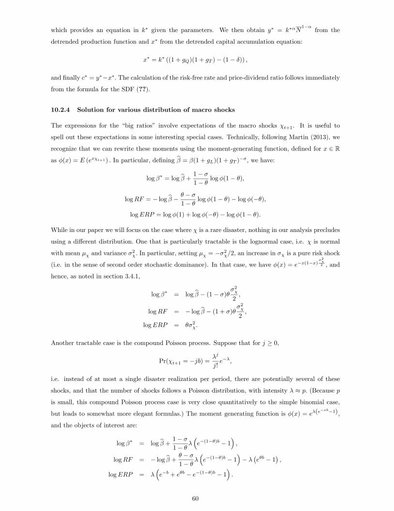
which provides an equation in k� given the parameters. We then obtain y� = k��N1��
from the
detrended production function and x� from the detrended capital accumulation equation:
x� = k� ((1 + gQ)(1 + gT )� (1� �)) ;
and �nally c� = y��x�: The calculation of the risk-free rate and price-dividend ratio follows immediately
from the formula for the SDF (??).
10.2.4 Solution for various distribution of macro shocks
The expressions for the �big ratios� involve expectations of the macro shocks �t+1. It is useful to
spell out these expectations in some interesting special cases. Technically, following Martin (2013), we
recognize that we can rewrite these moments using the moment-generating function, de�ned for x 2 R
as �(x) = E (ex�t+1) : In particular, de�ning b� = �(1 + gL)(1 + gT )��; we have:
log �� = log b� + 1� �1� � log �(1� �);
logRF = � log b� � � � �1� � log �(1� �)� log �(��);
logERP = log �(1) + log �(��)� log �(1� �):
While in our paper we will focus on the case where � is a rare disaster, nothing in our analysis precludes
using a di¤erent distribution. One that is particularly tractable is the lognormal case, i.e. � is normal
with mean �� and variance �2�: In particular, setting �� = ��2�=2, an increase in �� is a pure risk shock
(i.e. in the sense of second order stochastic dominance). In that case, we have �(x) = e�x(1�x)�2�2 ; and
hence, as noted in section 3.4.1,
log �� = log b� � (1� �)��2�2;
logRF = � log b� � (1 + �)��2�2;
logERP = ��2�:
Another tractable case is the compound Poisson process. Suppose that for j � 0;
Pr(�t+1 = �jb) =�j
j!e��;
i.e. instead of at most a single disaster realization per period, there are potentially several of these
shocks, and that the number of shocks follows a Poisson distribution, with intensity � � p: (Because p
is small, this compound Poisson process case is very close quantitatively to the simple binomial case,
but leads to somewhat more elegant formulas.) The moment generating function is �(x) = e�(e�xb�1);
and the objects of interest are:
log �� = log b� + 1� �1� � �
�e�(1��)b � 1
�;
logRF = � log b� + � � �1� � �
�e�(1��)b � 1
�� �
�e�b � 1
�;
logERP = ��e�b + e�b � e�(1��)b � 1
�:
60

It is straightforward to extend this calculation to the case of random size of shocks b, as in Kilic and
Wachter (2017).
In our application we will assume that�t+1 follows a three-point distribution, i.e.
�t+1 = 0 with probability 1� 2p;
�t+1 = log(1� b) with probability p;
�t+1 = log(1 + bH) with probability p;
where b and bH and are chosen so that E�e�+1
�= 1: The second state is a �disaster�: output and
consumption fall permanently by a factor 1� b: The third state is a �windfall�or �bonanza�state that
o¤sets the mean e¤ect of the disaster. One could also use a more traditional two-point process, without
the third state, which would then not satisfy E�e�+1
�= 1; and in that case a change in p would have
both a �rst moment and second moment e¤ect.s
61