Embed Size (px)
Citation preview

Accounting for Cross-
Country Income Differences:
Ten Years Later
BACKGROUND PAPER GOVERNANCE and THE LAW
Francesco Caselli London School of Economics

Disclaimer This background paper was prepared for the World Development Report 2017 Governance and the Law. It is made available here to communicate the results of the Bank’s work to the development community with the least possible delay. The manuscript of this paper therefore has not been prepared in accordance with the procedures appropriate to formally-edited texts. The findings, interpretations, and conclusions expressed in this paper do not necessarily reflect the views of The World Bank, its Board of Executive Directors, or the governments they represent. The World Bank does not guarantee the accuracy of the data included in this work. The boundaries, colors, denominations, and other information shown on any map in this work do not imply any judgment on the part of The World Bank concerning the legal status of any territory or the endorsement or acceptance of such boundaries.

Accounting for Cross-Country Income Differences:
Ten Years Later
Francesco Caselli∗
May 2016
1 Introduction
My 2005 survey of development accounting is often cited as motivation for studies at-
tempting to explain cross-country differences in the effi ciency with which capital and labor
are used [Caselli (2005)]. That study focused on a cross-section of countries observed in
the mid-1990s, so the conclusions from that effort are beginning to be a bit dated. In
addition, significant revisions of the data underlying the 2005 paper have been published.
Last but not least, in the intervening years I have become aware of ways in which the
original methodology can be usefully improved and extended. Hence the present update
and upgrade of the original paper.1 This paper focuses on data (mostly) from 2005 and
improves on the original methodology in several dimensions.
Development accounting compares differences in income per worker between developing
and developed countries to counter-factual differences attributable to observable compo-
∗London School of Economics, Centre for Macroeconomics, BREAD, CEP, CEPR, and NBER. Email:
[email protected]. This paper was written as a background paper for the World Bank’s World Develop-
ment Report. I am very grateful to Federico Rossi for excellent research assistance.1Besides the survey of development accounting, the 2005 paper also contained calculations aimed at
assessing the role of sectoral effi ciency differences in overall effi ciency differences; and a study of non-neutral
tecnology differences. An “update and upgrade”of the latter is offered in Caselli (2016).
1

nents of physical and human capital. Such calculations can serve a useful preliminary
diagnostic role before engaging in deeper and more detailed explorations of the fundamen-
tal determinants of differences in income per worker. If differences in physical and human
capital —or capital gaps —are suffi cient to explain most of the difference in incomes, then
researchers and policy makers need to focus on factors holding back investment (in ma-
chines and in humans). Instead, if differences in capital are insuffi cient to account for most
of the variation in income, one must conclude that developing countries are also hampered
by relatively low effi ciency at using their inputs - effi ciency gaps. The research and pol-
icy agenda would then have to focus on technology, allocative effi ciency, competition, and
other determinants of the effi cient use of capital.
I measure physical capital as an aggregate of reproducible and “natural”capital. Repro-
ducible capital includes equipment and structures, while natural capital primarily includes
subsoil resources, arable land, and timber. The inclusion of natural capital in the physical
capital stock, as applied to development accounting, is an innovation of the present paper.
The importance of tracking the contribution of natural capital to production is illustrated
by Caselli and Feyrer (2007).
My preferred measure of human capital is based on a “Mincerian”framework, where the
key inputs are schooling (years of education), health (as proxied by the adult survival rate),
and cognitive skills (as proxied by test score results). However because of limitations in the
coverage of the test results, I also present results where human capital is only measured
from years of schooling and health. It turns out that, at least in my preferred calibration,
the addition or omission of cognitive skills (as measured by test scores) does not greatly
affect the quantitative results.
Given measures of physical capital gaps, as well gaps in the components of human
capital, development-accounting uses a calibration to map these gaps into counter-factual
income gaps, or the income gaps that would be observed based on differences in human and
capital endowments only. Because these counterfactual incomes are bundles of physical
and human capital, I refer to the ratio of a country’s counterfactual incomes to the US
counterfactual income as relative capital.
I present results from two alternative calibrations, a “baseline” calibration and an
“aggressive”calibration. The baseline calibration makes use of the existing body of mi-
2

croeconomic estimates of the Mincerian framework in the way that most closely fits the
theoretical framework of development accounting. As it turns out, this leads to coeffi cients
for the mapping from the components of human capital to the index of human capital that
are substantially lower than in much existing work in development accounting - leading to
relatively smaller estimated capital gaps and, correspondingly, larger effi ciency gaps. The
aggressive calibration thus uses more conventional figures as a robustness check.
Under both the benchmark and the aggressive calibration I find very large effi ciency
gaps. In the benchmark calibration, countries in the bottom decile of the world income
distribution use their inputs only about 10% as effi ciently as the US; countries in the second
decile are less than 20% as effi cient; at the third it’s only little above 20%, and so on. The
effi ciency of countries in the 9th decile of the income distribution is roughly 90% of the
US level. The aggressive calibration implies higher relative effi ciency, but the gaps are still
huge. For example at the 3rd decile of the income distribution effi ciency is 30% of the US
level (against 20% in the benchmark calibration).
In assessing this evidence, it is essential to bear in mind that effi ciency gaps contribute
to income disparity both directly —as they mean that poorer countries get less out of their
capital —and indirectly —since much of the capital gap itself is likely due to diminished
incentives to invest in equipment, structure, schooling, and health caused by low effi ciency.
The consequences of closing the effi ciency gap would correspondingly be far reaching.
2 Conceptual Framework
The analytical tool at the core of development accounting is the aggregate production func-
tion. The aggregate production function maps aggregate input quantities into output. The
main inputs considered are physical capital and human capital. The empirical literature
so far has failed to uncover compelling evidence that aggregate input quantities deliver
large external economies, so it is usually deemed safe to assume constant returns to scale.2
Given this assumption, one can express the production function in intensive form, i.e. by
2See, e.g. Iranzo and Peri (2009) for a recent review and some new evidence on the quantitative
significance of schooling externalities.
3

specifying all input and output quantities in per worker terms. In order to construct coun-
terfactual incomes a functional form is needed. Existing evidence suggests that the share
of capital in income does not vary systematically with the level of development, or with
factor endowments [Gollin (2002)]. Hence, most practitioners of development accounting
opt for a Cobb-Douglas specification. In sum, the production function for country i is
yi = Aikαi h
1−αi , (1)
where y is output per worker, k is physical capital per worker, h is human capital per
worker (quality-adjusted labor), and A captures unmeasured/unobservable factors that
contribute to differences in output per worker.
The term A is subject to much speculation and controversy. Practitioners refer to it as
total factor productivity, technology, a measure of our ignorance, etc. Here I will refer to
it as “effi ciency”. Countries with a larger A are countries that, for whatever reasons, are
more effi cient users of their physical and human capital.
The goal of development accounting is to assess the relative importance of effi ciency
differences and physical and human capital differences in producing the differences in
income per worker we observe in the data. To this end, one constructs counterfactual
incomes, or capital bundles,
yi = kαi h1−αi , (2)
which are based exclusively on the observable inputs. Differences in these capital bundles
are then compared to income differences. If counter-factual and actual income differences
are similar, then observable factors are able to account for the bulk of the variation in
income. If they are quite different, then differences in effi ciency are important. Establishing
how significant effi ciency differences are has important repercussions both for research and
for policy.
In order to construct the counterfactual ys we need to construct measures of ki and
hi, as well as to calibrate the capital-share parameter α. Standard practice sets the latter
to 0.33, and we stick to this practice throughout the main body of the paper. In the
appendix I present robustness checks using a larger capital share, i.e. 0.40. This higher
share implies somewhat larger capital gaps and somewhat smaller effi ciency gaps, though
4
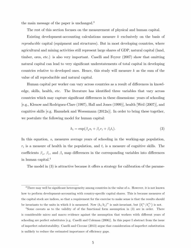
the main message of the paper is unchanged.3
The rest of this section focuses on the measurement of physical and human capital.
Existing development-accounting calculations measure k exclusively on the basis of
reproducible capital (equipment and structures). But in most developing countries, where
agricultural and mining activities still represent large shares of GDP, natural capital (land,
timber, ores, etc.) is also very important. Caselli and Feyrer (2007) show that omitting
natural capital can lead to very significant understatements of total capital in developing
countries relative to developed ones. Hence, this study will measure k as the sum of the
value of all reproducible and natural capital.
Human capital per worker can vary across countries as a result of differences in knowl-
edge, skills, health, etc. The literature has identified three variables that vary across
countries which may capture significant differences in these dimensions: years of schooling
[e.g., Klenow and Rodriguez-Clare (1997), Hall and Jones (1999)], health [Weil (2007)], and
cognitive skills [e.g. Hanushek and Woessmann (2012a)]. In order to bring these together,
we postulate the following model for human capital:
hi = exp(βssi + βrri + βtti). (3)
In this equation, si measures average years of schooling in the working-age population,
ri is a measure of health in the population, and ti is a measure of cognitive skills. The
coeffi cients βs, βr, and βt map differences in the corresponding variables into differences
in human capital.4
The model in (3) is attractive because it offers a strategy for calibration of the parame-
3There may well be significant heterogeneity among countries in the value of α. However, it is not known
how to perform development-accounting with country-specific capital shares. This is because measures of
the capital stock are indices, so that a requirement for the exercise to make sense is that the results should
be invariants to the units in which k is measured. Now (ki/kj)α is unit-invariant, but
(kαii /k
αjj
)is not.
4Some caveats as to the validity of of the functional form assumption in (3) are in order. There
is considerable micro and macro evidence against the assumption that workers wiith different years of
schooling are perfect substitutes [e.g. Caselli and Coleman (2006)]. In this paper I abstract from the issue
of imperfect substitutability. Caselli and Ciccone (2013) argue that consideration of imperfect substitution
is unlikely to reduce the estimated importance of effi ciency gaps.
5

ters βs, βr, and βt. In particular, combining (1), (3), and an assumption that wages are
proportional to the marginal productivity of labor, we obtain the “Mincerian”formulation
log(wij) = αi + βssij + βrrij + βttij, (4)
where wij (sij, etc.) is the wage (years of schooling, etc.) of worker j in country i, and
αi is a country-specific term.5 This suggests that using within-country variation in wages,
schooling, health, and cognitive skills one might in principle identify the coeffi cients β.
In practice, there are severe limitations in following this strategy, that we discuss after
introducing the data.
3 Data
I work with a sample of 128 countries for which I have data for y, k, s, and r, all observed
in 2005. These data are an extract from a dataset I developed in Caselli (2016), which
contains details of construction and definitions. I treat the USA as the benchmark country.
Since all of the variables enter the calculations either as ratios or as differences to US values,
this effectively means that there are 127 data points. When including test score estimates,
the number of data points will drop to 54.
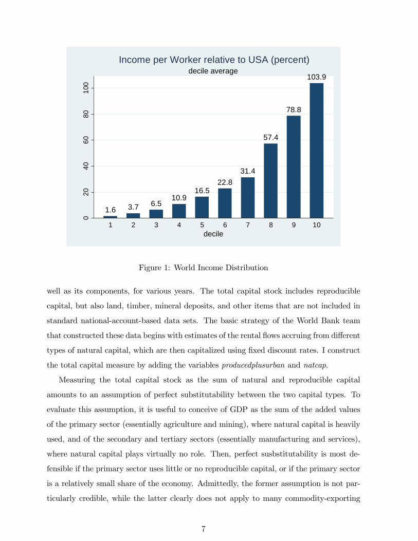
Per-worker income yi is variable rgdpwok from version 7.1 of the Penn World Tables
(PWT71). Figure 1 depicts the distribution of income per worker relative to the USA,
or yi/yUS. Countries are grouped by decile, and the bars represent the decile mean. The
colossal income gaps shown in the figure are well known, of course. In the bottom decile
income is two orders of magnitudes lower than in the US. At the median, it’s still one order
of magnitude. Standards of living remotely comparable to the US only begin to appear in
the 9th decile.
World Bank (2012) presents cross-sectional estimates of the total capital stock, k, as
5Note that this approach to the measurement of human capital is robust to a broad range of deviations
from perfect competition. In particular, the wage does not need to equal the marginal productivity of
labour, but just be proportional to it. Many models of monopsony in labor markets and monopolistic
competition have this property.
6
1.6 3.7 6.510.9
16.522.8
31.4
57.4
78.8
103.90
2040
6080
100
1 2 3 4 5 6 7 8 9 10decile
decile averageIncome per Worker relative to USA (percent)
Figure 1: World Income Distribution
well as its components, for various years. The total capital stock includes reproducible
capital, but also land, timber, mineral deposits, and other items that are not included in
standard national-account-based data sets. The basic strategy of the World Bank team
that constructed these data begins with estimates of the rental flows accruing from different
types of natural capital, which are then capitalized using fixed discount rates. I construct
the total capital measure by adding the variables producedplusurban and natcap.
Measuring the total capital stock as the sum of natural and reproducible capital
amounts to an assumption of perfect substitutability between the two capital types. To
evaluate this assumption, it is useful to conceive of GDP as the sum of the added values
of the primary sector (essentially agriculture and mining), where natural capital is heavily
used, and of the secondary and tertiary sectors (essentially manufacturing and services),
where natural capital plays virtually no role. Then, perfect susbstitutability is most de-
fensible if the primary sector uses little or no reproducible capital, or if the primary sector
is a relatively small share of the economy. Admittedly, the former assumption is not par-
ticularly credible, while the latter clearly does not apply to many commodity-exporting
7

2.4 3.4 7.0 10.8 13.820.9
29.0
66.3
98.7
152.20
5010
015
0
1 2 3 4 5 6 7 8 9 10income decile
average by income decilePhysical Capital per Worker relative to USA (percent)
Figure 2: Endowments of Physical Capital
countries. Intuitively, though, this should result in an overestimate of the capital gap in
commodity-exporting countries, and consequently an underestimate of the effi ciency gap.
If the primary sector is large, and reproducible capital plays a significant role in the primary
sector, reproducible capital and natural capital should boost each other’s productivity, re-
sulting in a larger capital bundle than in the case they are perfect substitutes. In other
words, by assuming perfect substitutability we are underestimating the total contribution
of commodity exporters than in the richer, benchmark country.
Figure 2 shows total (reproducible plus natural) capital per worker relative to the US,
ki/kUS, by relative-income decile. I.e., countries continue to be ranked by their relative
income, as in Figure 1, and not by their relative capital. The same format will be used in
all subsequent figures. The figure shows that physical-capital gaps are broadly comparable
to income gaps: average relative physical capital in the various income deciles tends to be
of a similar order of magnitude as average relative income.
For average years of schooling in the working-age population (which is defined as be-
tween 15 and 99 years of age) I rely on Barro and Lee (2013). Note from equation (3)
8

9.2
7.97.0
4.95.7
4.53.9
2.6 2.7 2.9
10
86
42
0
1 2 3 4 5 6 7 8 9 10income decile
average by income decileDifferences in Years of Schooling with USA
Figure 3: Schooling by Income Decle
that for the purposes of constructing relative human capital hi/hUS what is relevant is the
difference in years of schooling si − sUS. The same will be true for r and t. Accordingly,
in Figure 3 I plot schooling-year differences with the USA in 2005.
Schooling gaps with the USA are very substantial. In countries in the bottom income
decile the average workers has 9.2 fewer years of schooling. In the fifth decile, it is still 5.7
(though interestingly the 4th decile does a bit better, with 4.7). Remarkably, the schooling
gap with the USA remains quite substantial even at the top, with each of the top three
deciles showing a gap between 2.6 and 2.9 years.
As a proxy for the health status of the population, r, Weil (2007) proposes using
the adult survival rate. The adult survival rate is a statistic computed from age-specific
mortality rates at a point in time. It can be interpreted as the probability of reaching
the age of 60, conditional on having reached the age of 15, at current rates of age-specific
mortality. Since most mortality before age 60 is due to illness, the adult survival rate is a
reasonably good proxy for the overall health status of the population at a given point in
time. Relative to more direct measures of health, the advantage of the adult survival rate is
9
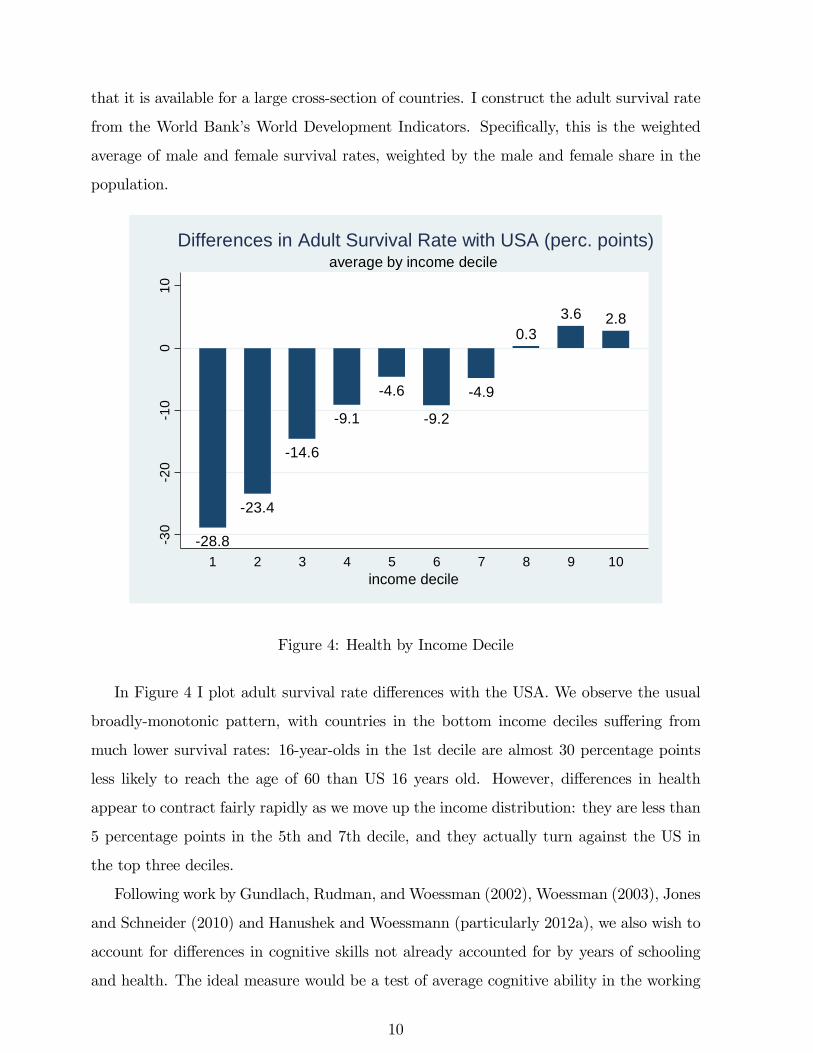
that it is available for a large cross-section of countries. I construct the adult survival rate
from the World Bank’s World Development Indicators. Specifically, this is the weighted
average of male and female survival rates, weighted by the male and female share in the
population.
28.8
23.4
14.6
9.1
4.6
9.2
4.9
0.33.6 2.8
30
20
10
010
1 2 3 4 5 6 7 8 9 10income decile
average by income decileDifferences in Adult Survival Rate with USA (perc. points)
Figure 4: Health by Income Decile
In Figure 4 I plot adult survival rate differences with the USA. We observe the usual
broadly-monotonic pattern, with countries in the bottom income deciles suffering from
much lower survival rates: 16-year-olds in the 1st decile are almost 30 percentage points
less likely to reach the age of 60 than US 16 years old. However, differences in health
appear to contract fairly rapidly as we move up the income distribution: they are less than
5 percentage points in the 5th and 7th decile, and they actually turn against the US in
the top three deciles.
Following work by Gundlach, Rudman, andWoessman (2002), Woessman (2003), Jones
and Schneider (2010) and Hanushek and Woessmann (particularly 2012a), we also wish to
account for differences in cognitive skills not already accounted for by years of schooling
and health. The ideal measure would be a test of average cognitive ability in the working
10

population. Hanushek and Zhang (2009) report estimates of one such test (the Interna-
tional Adult Literacy Survey (IALS)) for a dozen countries, but this is clearly too small a
sample to be useful here.
As a fallback, I rely on internationally comparable test scores taken by school-age
children. I will use scores from a science test administered in 2009 to 15 year olds by
PISA (Program for International Student Assessment). There are in principle several
other internationally-comparable tests (by subject matter, year of testing, and organization
testing) that could be used in alternative to or in combination with the 2009 PISA science
test. However there would be virtually no gain in country coverage by using or combining
with other years (the PISA tests of 2009 are the ones with the greatest participation).
Focusing only on one test bypasses potentially thorny issues of aggregation across years,
subjects, and methods of administration. Cross-country correlations in test results are
very high anyway, and very stable over time.6 Data on PISA test score results are from
the World Bank’s Education Statistics.
Needless to say measuring t by the above-described test scores is clearly very unsatis-
factory, as in most cases the tests reflect the cognitive skills of individuals who have not
joined the labor force as of 2005, much less those of the average worker. Implicitly, we are
interpreting test-score gaps in current children as proxies for test scores gaps in current
workers. If the US and the other countries in the sample have experienced different trends
in cognitive skills of children over the last few decades this assumption is problematic.
The 2009 PISA science tests are reported on a scale from 0 to 1000, and they are
normalized so that the average score among OECD countries (i.e. among all pupils taking
the test in this set of countries) is (approximately) 500 and the standard deviation is
(approximately) 100.7 Figure 5 shows test score differences ti− tUS for the countries which
6Repeating all my calculations using the PISA math scores yielded results that were virtually indistin-
guishable from those using the science test.7I say approximately in parenthesis because the normalization was applied to the 2006 wave of the
test. The 2009 test was graded to be comparable to the 2006 one. Hence, it is likely that the 2009 mean
(standard deviation) will have drifted somewhat away from 500 (100) - though probably not by much. The
PISA math and reading tests were normalized in 2000 and 2003, respectively, so their mean and standard
deviation are more likely to have drifted away from the initial benchmark. This is one reason why I use
11

145.9
111.399.0
87.7
30.114.0
16.24.6
150
100
50
050
1 2 3 4 5 6 7 8 9 10income decile
average by income decileDifferences in Science Test Scores with USA
Figure 5: Cognitive Skills by Income Decile
took part in the test. The poorest country in the sample to report a test score is the country
at the 24th percentile of the relative income distribution, so I cannot plot cognitive-skill
differences from the bottom two deciles.8
Differences in PISA scores are very significant. In the third and fourth decile the gap
between the average student and the average US student exceeds the standard deviation
among OECD students. In the fifth and sixth deciles the gap is still similar to the OECD
standard deviation. On the other hand countries in the top two income deciles outperform
the US.
the science test for my baseline calculations.8Recall that I have complete data on income, physical capital, years of scholing, and survival rates
for my smaple of 128 countries, but only 58 countries with test scores. This also implies that the decile
averages in Figure 5 are typically based on a subset of the countries that populate the decile.
12
4 Calibration
The last, and most diffi cult, step in producing counter-factual income gaps between US
and Latin America is to calibrate the coeffi cients βs, βr, and βt. As discussed, equation
(4) indicates that, using within country data on w, s, r, and t, one could in principle
identify these coeffi cients by running an extended Mincerian regression for log-wages. In
implementing this plan, we are confronted with (at least) two important problems.
The first problem is that one of the explanatory variables, the adult survival rate
r, by definition does not vary within countries. Estimating βr directly is therefore a
logical impossibility. To solve this problem Weil (2007) notices that, in the time series
(for a sample of ten countries for which the necessary data is available), there is a fairly
tight relationship between the adult survival rate and average height. In other words, he
postulates ci = αc+γcri, where ci is average height and the coeffi cient γc is estimated from
the above-mentioned time series relation (he obtains a coeffi cient of 19.2 in his preferred
specification). Since height does vary within countries as well as between countries, this
opens the way to identifying βr by means of the Mincerian regression
log(wij) = αi + βssij + βccij + βttij,
where βr = βcγc.9
The second problem is that measures of t are not consistent at the macro and at the
micro level. In particular, while we do have micro data sets reporting both results from
tests of cognitive skills and wages, the test in question is simply a different test from the
tests we have available at the level of the cross-section of countries. Call the alternative test
available at the micro level d. Once again the solution is to assume a linear relationship
di = γdti. The difference with the case of height-survival rate is that, as far as I know, there
is no way to check the empirical plausibility of this assumption. Given the assumed linear
relationship, one can back out γd as the ratio of the within country standard deviation of
9Needless to say if we had cross-country data on average height there would be no need to use the
survival rate at all.
13

dij and tij. With γd at hand, one can back out βt from the modified Mincerian regression
log(wij) = αi + βssij + βccij + βddij, (5)
using βt = βdγd.
In choosing values for βs, βc, and βd from the literature it is highly desirable to focus on
microeconomic estimates of equation (5) that include all three right-hand variables. This
is because s, c, and d are well-known to be highly positively correlated.10 Hence, any OLS
estimate of one of the coeffi cients from a regression that omits one or two of the other two
variables will be biased upward.11
A search of the literature yielded one and only one study reporting all three coeffi cients
from equation (5). Vogl (2014) uses the two waves (2002 and 2005) of the nationally-
representative Mexican Family Life Survey to estimate (5) on a subsample of men aged
25-65. In his study, w is measured as hourly earnings, s as years of schooling, c is in
centimeters, and d is the respondent’s score on a cognitive-skill test administered at the
time of the survey.12 The cognitive skill measure is scaled so its standard deviation in the
Mexican population is 1.13
The coeffi cients reported by Vogl are as follows (see his Table 4, column 7). The return
to schooling βs is 0.072, which can be plugged directly in equation (3). The “return to
height”βc is 0.013. Hence, the coeffi cient associated with the adult survival rate in (3)
is 0.013 x 19.2 = 0.25, where I have used Weil’s mapping between height and the adult
survival rate. Finally, the reported return to cognitive skills βd is 0.011. Since the standard
deviation of d is one by construction, and the standard deviation of the 2009 Science PISA
test in Mexico is 77, the implied coeffi cient on the PISA test for the purposes of constructing
10See, e.g., the literature review in Vogl (2014).11An alternative would be to use IV estimates of the βs, but instruments for the variables on the right
hand side of equation 5 are often somewhat controversial - especially for height and cognitive skills.12The test is the short-form Raven’s Progressive Matrices Test.13Needless to say there are aspects of Vogl’s treatment that imply the regressions he runs are not a
perfect fit for the conceptual framework of the paper. It may have been preferable for our pusposes to
include both men and women. He also controls for ethnicity, age, and age squared, which do not feature
in my framework. Finally, he notes that the Raven’s core is a coarse measure of cognitive skills, giving
raise to concerns with attenuation bias (more on this below).
14
h is 0.011/77=0.00014.
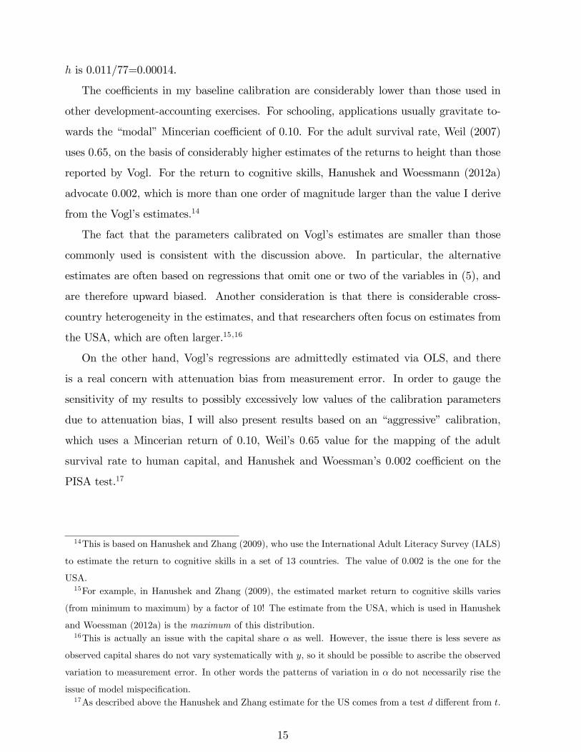
The coeffi cients in my baseline calibration are considerably lower than those used in
other development-accounting exercises. For schooling, applications usually gravitate to-
wards the “modal”Mincerian coeffi cient of 0.10. For the adult survival rate, Weil (2007)
uses 0.65, on the basis of considerably higher estimates of the returns to height than those
reported by Vogl. For the return to cognitive skills, Hanushek and Woessmann (2012a)
advocate 0.002, which is more than one order of magnitude larger than the value I derive
from the Vogl’s estimates.14
The fact that the parameters calibrated on Vogl’s estimates are smaller than those
commonly used is consistent with the discussion above. In particular, the alternative
estimates are often based on regressions that omit one or two of the variables in (5), and
are therefore upward biased. Another consideration is that there is considerable cross-
country heterogeneity in the estimates, and that researchers often focus on estimates from
the USA, which are often larger.15 ,16
On the other hand, Vogl’s regressions are admittedly estimated via OLS, and there
is a real concern with attenuation bias from measurement error. In order to gauge the
sensitivity of my results to possibly excessively low values of the calibration parameters
due to attenuation bias, I will also present results based on an “aggressive” calibration,
which uses a Mincerian return of 0.10, Weil’s 0.65 value for the mapping of the adult
survival rate to human capital, and Hanushek and Woessman’s 0.002 coeffi cient on the
PISA test.17
14This is based on Hanushek and Zhang (2009), who use the International Adult Literacy Survey (IALS)
to estimate the return to cognitive skills in a set of 13 countries. The value of 0.002 is the one for the
USA.15For example, in Hanushek and Zhang (2009), the estimated market return to cognitive skills varies
(from minimum to maximum) by a factor of 10! The estimate from the USA, which is used in Hanushek
and Woessman (2012a) is the maximum of this distribution.16This is actually an issue with the capital share α as well. However, the issue there is less severe as
observed capital shares do not vary systematically with y, so it should be possible to ascribe the observed
variation to measurement error. In other words the patterns of variation in α do not necessarily rise the
issue of model mispecification.17As described above the Hanushek and Zhang estimate for the US comes from a test d different from t.
15
020
4060
80
1 2 3 4 5 6 7 8 9 10income decile
average by income decileHuman Capital Relative to USA (percent)
accounting for cognitive skillsnot accounting for cognitive skills
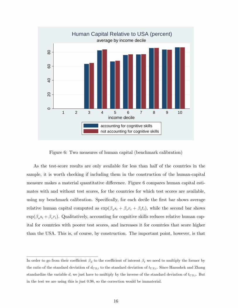
Figure 6: Two measures of human capital (benchmark calibration)
As the test-score results are only available for less than half of the countries in the
sample, it is worth checking if including them in the construction of the human-capital
measure makes a material quantitative difference. Figure 6 compares human capital esti-
mates with and without test scores, for the countries for which test scores are available,
using my benchmark calibration. Specifically, for each decile the first bar shows average
relative human capital computed as exp(βssi + βrri + βtti), while the second bar shows
exp(βssi+βrri). Qualitatively, accounting for cognitive skills reduces relative human cap-
ital for countries with poorer test scores, and increases it for countries that score higher
than the USA. This is, of course, by construction. The important point, however, is that
In order to go from their coeffi cient βd to the coeffi cient of interest βt we need to multiply the former by
the ratio of the standard deviation of dUS,i to the standard deviation of tUS,i. Since Hanushek and Zhang
standardize the variable d, we just have to multiply by the inverse of the standard deviation of tUS,i. But
in the test we are using this is just 0.98, so the correction would be immaterial.
16

the differences between accounting and not-accounting for cognitive skills is minuscule.
This is of course a consequence of the very small coeffi cient on cognitive skills from Vogl’s
estimates.
In light of the very small difference between relative human capital measures that
account and do not account for cognitive skills, it does not seem worthwhile to give up on
more than half of the sample to include cognitive skills in the measure of human capital
- at least when using the benchmark calibration. From now on, therefore, my benchmark
calculations will drop the test-score correction. Figure 7 shows relative human capital on
the full sample.
49.354.8
59.6
70.166.6
71.875.6
83.9 83.7 82.8
020
4060
80
1 2 3 4 5 6 7 8 9 10income decile
average by income decileHuman Capital per Worker relative to USA (percent)
Figure 7: Human Capital in the Full Sample
Relative human capital is still broadly increasing in income. However, human-capital
gaps do not appear as large as physical-capital gaps. The countries in the bottom income
decile have half as much as the human capital of the USA. The distribution of relative
human-capital is also remarkably compressed, ranging from just shy of 50% to just over
80%. Of course the fact that human-capital gaps are comparatively small does not imply
that human capital contributes little to income gaps, as the elasticity of income to human
17

capital is twice as large as its elasticity to physical capital.
020
4060
80
1 2 3 4 5 6 7 8 9 10income decile
average by income decile aggressive calibrationHuman Capital Relative to USA (percent)
accounting for cognitive skillsnot accounting for cognitive skills
Figure 8: Aggressive Calibration
8 compares human capital estimates with and without test scores, using the aggressive
calibration. The differences are quite significant this time. In the 3rd income decile relative
human capital is 10 percentage points lower when accounting for cognitive skills; in the 4th
decile, almost 20 percentage points. It is clear that when using the aggressive calibration
we cannot ignore test scores. Accordingly, when reporting results from the aggressive
calibration I will focus only on the subsample of countries which participated in the PISA
science test. Not surprisingly, using the aggressive calibration results in significantly lower
relative human capital, since the impact of differentials in schooling, health, and cognitive
skills is magnified.
5 Results
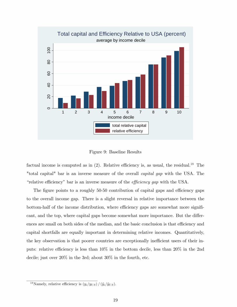
My baseline results are presented in Figure 9, which shows average counter-factual income
(labeled “total capital”) and effi ciency relative to the USA by income decile. Counter-
18
020
4060
8010
0
1 2 3 4 5 6 7 8 9 10income decile
average by income decileTotal capital and Efficiency Relative to USA (percent)
total relative capitalrelative efficiency
Figure 9: Baseline Results
factual income is computed as in (2). Relative effi ciency is, as usual, the residual.18 The
"total capital" bar is an inverse measure of the overall capital gap with the USA. The
“relative effi ciency”bar is an inverse measure of the effi ciency gap with the USA.
The figure points to a roughly 50-50 contribution of capital gaps and effi ciency gaps
to the overall income gap. There is a slight reversal in relative importance between the
bottom-half of the income distribution, where effi ciency gaps are somewhat more signifi-
cant, and the top, where capital gaps become somewhat more importance. But the differ-
ences are small on both sides of the median, and the basic conclusion is that effi ciency and
capital shortfalls are equally important in determining relative incomes. Quantitatively,
the key observation is that poorer countries are exceptionally ineffi cient users of their in-
puts: relative effi ciency is less than 10% in the bottom decile, less than 20% in the 2nd
decile; just over 20% in the 3rd; about 30% in the fourth, etc.
18Namely, relative effi ciency is (yi/yUS) / (yi/yUS).
19

020
4060
8010
0
1 2 3 4 5 6 7 8 9 10income decile
average by income decile aggressive calibrationTotal capital and Efficiency Relative to USA (percent)
total relative capitalrelative efficiency
Figure 10: Robustness to Aggressive Calibration
Figure 10 is analogous to Figure 9, but uses the aggressive calibration instead. Recall
that when using the aggressive calibration, we have to include the cognitive-test scores
and, as a consequence, we lose many observations. As expected, using larger parameters
in the mapping from schooling years, health, and test scores leads to a considerable decline
in relative capital. As a result, the relative contribution of capital gaps is now larger than
the contribution of effi ciency gaps for all income deciles. Nevertheless, huge effi ciency gaps
persist even under the aggressive calibration. The average effi ciency of the 3rd decile is
30%; in the 4th decile is less than 40%.
In order to fully appreciate the importance of these effi ciency gaps it is crucial to note
that, under almost any imaginable set of circumstances, physical (specifically, reproducible)
and human capital accumulation respond to a country’s level of effi ciency. The higher A
the higher the marginal productivity of capital, leading to enhanced incentives to invest
in equipment and structure, schooling, etc. While quantifying this effect is diffi cult, most
theoretical frameworks would lead one to expect it to be large. Hence, it is legitimate to
20
conjecture that a significant fraction of the capital gap may be due to the effi ciency gap.19
6 Implications and Conclusions
There is huge inequality in income per worker between the countries of theWorld: countries
in the bottom decile are about 100 times less productive than the USA, and substantial
differences persist all of the way up to the higher percentiles. A development-accounting
calculation reveals that both capital gaps and effi ciency gaps contribute roughly equally
to this overall productivity gap. Hence, poor countries are poorer both because they exert
less effort in accumulating productive factors, and because they use these factors much
less effi ciently. Reducing these effi ciency gaps would reduce overall productivity gaps both
directly and indirectly, since much of the capital gap is likely due to the effi ciency gap
itself: closing the effi ciency gap would stimulate investment at rates potentially capable of
closing the capital gap as well.
These conclusions are contingent on the quality of the underlying macroeconomic data.
There is growing concern about the quality and reliability of the PPP national-account
figures in the Penn World Tables and similar data sets [e.g. Johnson et al. (2013)]. Similar
concerns apply, no doubt, to our proxies for human capital as well (as already discussed
particularly in the context of cognitive skills). It is true that such concerns are most often
voiced in the context of implied comparisons of changes, especially over short time spans:
cross-country comparisons of levels reveal such gigantic differences (as seen above) that
they seem unlikely to be entirely dominated by noise. Still, exclusive reliance on these
macro data is highly inadvisable.
Fortunately, it is also increasingly unnecessary. The increasing availability of firm
level data sets, particularly when matched with employee-level information (e.g. about
schooling), provides an opportunity to supplement the macro picture with microeconomic
19In principle, one might also argue for a reverse direction of causation, with larger physical and human-
capital stocks leading to higher effi ciency. In particular, this would be true if the model was misspecified,
and there were large externalities. But as already mentioned the empirical literature has not to date
uncovered significant evidence of externalities in physical and human capital.
21
productivity estimates comparable across countries.
The benefit of producing such micro productivity estimates is by no means limited to
permitting to check the robustness of conclusions concerning average capital and effi ciency
gaps - though this benefit alone is suffi cient to make such exercises worthwhile. An ad-
ditional benefit is to uncover information on the within country distribution of physical
capital, human capital, and effi ciency. A relatively concentrated distribution would sug-
gest that effi ciency gaps are mostly due to aggregate, macroeconomic factors that affect
all firms fairly equally (e.g. impediment to technology diffusion from other countries). A
very dispersed distribution, with some firms close to the world technology frontier, would
be more consistent with allocative frictions that prevent capital and labor to flow to the
more effi cient/talented managers.
More generally, firm-level data is likely to prove essential in the quest for the deter-
minants of the large effi ciency gaps revealed by the development-accounting calculation.
After all, (in-)effi ciency is —by definition —a firm-level phenomenon. Most of the most
plausible possible explanations for the effi ciency gap are microeconomic in nature —whether
it is about firms unable to adapt technologies developed in more technologically-advanced
countries, failures in the market for managers and/or capital, frictions in the matching
process for workers, etc. It seems implausible that evidence for or against these mecha-
nisms can be found in the macro data. Yet understanding the sources of poor countries’
effi ciency gaps is unquestionably the most urgent task for those who want to design policies
aimed at closing the income gaps.
22

References
Barro and Lee (2013): "A New Data Set of Educational Attainment in the World,
1950-2010." Journal of Development Economics.
Caselli, F. (2005): “Accounting for cross-Country Income Differences,” in Philippe
Aghion and Stephen Durlauf (eds.), Handbook of Economic Growth, Volume 1A, 679-741,
Elsevier.
Caselli, F. (2016): Technology Differences over Space and Time”Princeton University
Press.
Caselli, Francesco, and Antonio Ciccone (2013): “The Contribution of Schooling in
Development Accounting: Results from a Nonparametric Upper Bound.”Journal of De-
velopment Economics.
Caselli, Francesco and Coleman, John Wilbur II, 2006. "The World Technology Fron-
tier." American Economic Review, 96, pp. 499-522.
Caselli, Francesco, and James Feyrer, 2007. "The Marginal Product of Capital." Quar-
terly Journal of Economics, 122, pp. 535-568.
Gollin, Douglas, 2002. "Getting Income Shares Right." Journal of Political Economy,
110, pp. 458-474.
Gundlach, Rudman, and Woessman (2002): “Second Thougths on Development Ac-
counting,”Applied Economics, 34, 1359-69.
Hall, Robert and Charles Jones, 1999. "Why Do Some Countries Produce So Much
More Output Per Worker Than Others?" Quarterly Journal of Economics, 114, pp. 83-116
Hanusheck, Eric, and Ludger Woessman (2012a): "Schooling, Educational Achieve-
ment, and the Latin American Growth Puzzle", Journal of Development Economics 99
(2), 497-512,
Hanushek, Eric A.,Woessmann, Ludger, (2012b). Do better schools lead to more
growth? Cognitive skills, economic outcomes, and causation. Journal of Economic Growth.
Hanushek, Eric and Lei Zhang (2009): “Quality-Consistent Estimates of International
Schooling and Skill Gradients,”Journal of Human Capital, 2009, 3(2), 107-43.
Iranzo, Susana and Giovanni Peri, 2009. "Schooling Externalities, Technology, and
Productivity: Theory and Evidence from US States." Review of Economics and Statistics,
91, pp. 420-431
23
Johnson, Simon, William Larson, Chris Papageorgiou, and Arvind Subramanian (2013):
“Is Newer Better? Penn World Table Revisions and Their Impact on Growth Estimates,”
Journal of Monetary Economics, March 2013.
Klenow, Peter, and Andres Rodriguez-Claire, 1997. "The Neoclassical Revival in
Growth Economics: Has It Gone Too Far?". In NBER Macroeconomic Annual, MIT
Press
Vogl, Tom S. (2014): “Height, Skills, and labor market outcomes in Mexico,”Journal
of Development Economics, 107, 84-96.
Weil, David, 2007. “Accounting for the Effect of Health on Economic Growth.”Quarterly
Journal of Economics, 122, pp.1265-1306.
Woessman, Rudiger (2003): “Specifying Human Capital,” Journal of Economic Sur-
veys, 17, 3, 239-270.
World Bank (2012): The Changing Wealth of Nations.
24


