Embed Size (px)
Citation preview

Accounting Data, Market Values, and the Cross Section of Expected Returns Worldwide
Akash Chattopadhyay Matthew R. Lyle Charles C.Y. Wang
Working Paper 15-092

Working Paper 15-092
Copyright © 2015, 2016 by Akash Chattopadhyay, Matthew R. Lyle, and Charles C.Y. Wang
Working papers are in draft form. This working paper is distributed for purposes of comment and discussion only. It may
not be reproduced without permission of the copyright holder. Copies of working papers are available from the author.
Accounting Data, Market Values, and the Cross Section of Expected Returns Worldwide
Akash Chattopadhyay Harvard Business School
Matthew R. Lyle Kellogg School of Management
Charles C.Y. Wang Harvard Business School

Accounting Data, Market Values, and the CrossSection of Expected Returns Worldwide
Akash ChattopadhyayHarvard Business School
Matthew R. LyleKellogg School of Management
Charles C.Y. Wang∗
Harvard Business School
January 2016
Abstract
Under fairly general assumptions, expected stock returns are a linear combinationof two accounting-based characteristics—book to market and ROE. Empirical es-timates based on this relation predict the cross section of out-of-sample returnsin 26 of 29 international equity markets, with a highly significant average slopecoefficient of 1.05. In sharp contrast, standard factor-model-based proxies fail toexhibit predictive power internationally. We show analytically and empirically thatthe importance of ROE in forecasting returns depends on the quality of account-ing information. Overall, a tractable accounting-based valuation model provides aunifying framework for obtaining reliable proxies of expected returns worldwide.
Keywords: Expected returns, discount rates, fundamental valuation, present value,information quality, international equity markets.
JEL: D83, G12, G14, M41
∗Chattopadhyay ([email protected]) is a doctoral candidate in Accounting and Managementat Harvard Business School. Lyle ([email protected]) is Assistant Professor of Ac-counting Information and Management and The Lawrence Revsine Research Fellow at Kellogg Schoolof Management. Wang ([email protected]) is Assistant Professor of Business Administrationat Harvard Business School. For helpful comments and suggestions, we are grateful to S.P. Kothari(the Editor), Ryan Buell, Craig Chapman, Peter Easton, Ian Gow, Joseph Gerakos (AAA discussant),Jeremiah Green (FARS discussant), Daniel Malter, Bob Magee, Jim Naughton, Scott Richardson (JAEdiscussant), Tatiana Sandino, Pian Shu, Phil Stocken, Suraj Srinivasan, Tuomo Vuolteenaho, BeverlyWalther, Clare Wang, James Zeitler, Lu Zhang, and to workshop participants at University of Alberta,Arizona State University, Citadel Quantitative Research, Duke University, Haskayne School of Business,University of Illinois at Chicago, Kellogg School of Management, University of Miami, National ChengchiUniversity, as well as participants of the 2015 FARS conference, Minnesota Empirical Accounting Re-search Conference, AAA annual conference, and Journal of Accounting and Economics Conference. Wethank Kyle Thomas for excellent research assistance. Lyle is grateful for generous funding providedthrough the Lawrence Revsine Research Fellowship.

Accounting Data, Market Values, and Expected Returns Worldwide 1
1 Introduction
Estimating expected returns has been a centerpiece in financial economics since at
least the derivation of the CAPM (Sharpe, 1964). Over the past thirty years, under-
standing what drives the variation in expected returns has been the central organizing
theoretical and empirical question in asset pricing (Cochrane, 2011). Capital markets
research in accounting has also developed a large and growing literature examining how
different firm attributes or policies—e.g., disclosure policies (Botosan, 1997), audit quality
(Chen, Chen, Lobo, and Wang, 2011), or corporate governance and regulatory institutions
(Hail and Leuz, 2006)—affect expected returns.
Despite its importance, empirical research in this area remains problematic, and re-
sults are often controversial because the key dependent variable—expected returns—is
not directly observable, notoriously difficult to measure, and there is no well-accepted
standard for its estimation. We posit that such a standard should, by definition, produce
empirical proxies that on average forecast the cross-section of future returns and across
multiple equity markets. Despite extensive work on this measurement problem, to our
knowledge no such method exists.
Factor-based models, like the capital asset pricing model or the Fama and French
(1993) factor model, are unreliable proxies of ex ante expected returns as they fail to
exhibit out-of-sample predictive ability in the U.S. (Lee, So, and Wang, 2014; Lyle and
Wang, 2015). The accounting literature’s development of the implied cost of capital
(ICC) class of expected return proxies (ERPs), as an alternative to factor-based proxies,
have so far failed to produce a well-accepted standard.1 This may be in part due to the
restrictive assumptions that underlie ICC models (e.g., constant expected returns, ad-
hoc terminal growth assumptions), the difficulties in their implementation (e.g., solving
1Recent examples of papers that explore the performance of these and other expected-return proxiesinclude: Botosan and Plumlee (2005); Botosan, Plumlee, and Wen (2011); Easton and Monahan (2005);Lyle, Callen, and Elliott (2013); Lee et al. (2014); Lyle and Wang (2015); and Wang (2015).

Accounting Data, Market Values, and Expected Returns Worldwide 2
non-linear equations by numerical methods that may or may not converge, or that may
converge to multiple solutions), and, perhaps most saliently, the lack of evidence that
ICCs, in the cross section, line up well with expected returns (Easton and Monahan,
2005; Lee et al., 2014).
These empirical challenges are exacerbated in international settings (Lee, Ng, and
Swaminathan, 2009). Varying degrees in the integration with global markets, differences
in regulatory and governance institutions, the relative paucity of international data, and
differences in accounting reporting standards represent significant barriers to a uniform
standard or framework for estimating firm-level expected returns worldwide. Indeed,
prior work shows that factors known to explain the in-sample variation of returns in the
United States do not necessarily explain the cross section of returns in other markets
internationally (Fama and French, 2012; Hou, Karolyi, and Kho, 2011). It is perhaps
not surprising, therefore, that there is no consensus on a well-accepted and theoretically-
motivated standard for estimating firm-level expected returns, not only in the U.S. setting
but also across international markets.
Motivated by the above, this paper centers around the following research questions:
what is the role of accounting information in the measurement of expected returns, and
how does this role vary across different accounting regimes or systems? We show, both
analytically and empirically, that a simple and parsimonious accounting-based approach
can offer a step forward in addressing the long-standing challenge of measuring expected
returns. We derive, under fairly general assumptions, an accounting-based ERP that (i)
can forecast the cross-section of future returns worldwide, and (ii) lines up well with future
average returns. Our work validates and builds on, in three ways, the findings of Lyle
and Wang (2015) (subsequently referred to as LW15), who apply the log-linearization of
Vuolteenaho (2002) to derive a tractable model of time-varying expected rate of return
that is a linear function of the book-to-market ratio (BM) and return-on-equity (ROE).

Accounting Data, Market Values, and Expected Returns Worldwide 3
First, we show analytically that the accounting-based model of expected returns in
LW15 is quite robust and can be applied to a broader set of firms, including non-dividend-
paying firms. Like LW15, we show that a parsimonious solution for estimating firm-level
expected returns requires only a linear combination of two accounting-based character-
istics: BM and ROE. But we derive this solution under more generalized and milder
assumptions: 1) book values are expected to carry value-relevant information, and 2) ex-
pected growth rates in market and book are mean-reverting. Thus, we generalize LW15 by
showing that this linear relation between expected returns and accounting-based charac-
teristics holds even if firms do not pay dividends, rather than the assumption of firm-level
dividend payments implicit in the Vuolteenaho (2002) approach.2
Second, we extend and validate in an international setting the empirical findings of
LW15, who focus only on U.S. equities. Our simple accounting-based ERPs perform well
internationally: they significantly and reliably predict the cross section of stock returns in
26 of 29 equity markets worldwide. They also provide an unbiased estimate of expected
returns. Fama-MacBeth (FM) regression tests—regressing one-month-ahead returns on
ex-ante proxies of expected returns—yield an average predictive slope coefficient of 1.05
(relative to the benchmark of 1). For 21 (20) of the 29 countries the predictive slope is
not significantly different from 1 at the 10% (5%) level. Portfolio-based tests yield similar
conclusions.
Finally, we build upon LW15 by examining, both analytically and empirically, how
the quality of accounting information affects the relation between accounting numbers
and expected returns. By relating the accounting-based model of expected returns to a
dynamic information structure, we show analytically that, holding all other sources of
information constant, higher-quality accounting information—defined by lower measure-
2The log-linearization approach of Vuolteenaho (2002) requires that firms pay dividends. Moreover,the approach taken by standard accounting valuation models Ohlson (1995) and Feltham and Ohlson(1995) also implicitly require dividends, which allow accounting to play a role through the clean surplusrelation. Our approach circumvents this issue.

Accounting Data, Market Values, and Expected Returns Worldwide 4
ment error variance—increases the importance of ROE in determining expected returns.
These predictions are supported by our empirical tests. Relying on measures of country-
level earnings quality derived from Leuz, Nanda, and Wysocki (2003) and employing an
instrumental variables estimation strategy, we document that, all else equal, higher earn-
ings quality elevates the importance of ROE in inferring expected returns. Together, we
contribute to the literature i) by providing a simple accounting-based ERP that can be
applied to international markets and ii) by demonstrating how the quality of accounting
systems impacts the importance of accounting information in this proxy.
Our work relates to the large implied cost of capital literature in accounting (e.g.,
Botosan, 1997; Gebhardt, Lee, and Swaminathan, 2001; Claus and Thomas, 2001; Gode
and Mohanram, 2003; Easton, 2004) in that we also seek to infer expected returns im-
plied by observed stock prices and accounting data. Our approach, though similar in
principle, has several distinct practical advantages. Ours is motivated by a fairly general
valuation model that does not rely on dividends or clean surplus relation, is applicable to
broad classes of accounting systems, is easy to implement, and does not require solving
non-linear equations. Further, our ERPs line up well with the cross section of future
returns across international equity markets—i.e., obtain a slope coefficient close to 1 and
a constant coefficient close to 0 in regressions of future returns on ERPs.
Our paper is also related to the large body of research in accounting and finance
linking stock returns to firm characteristics.3 Our study differs from these in that we
contribute by showing whether and how investors can combine firm characteristics to
form ERPs that line up well with expected returns, a subject that has received relatively
little (but growing) attention (e.g., Lewellen, 2015; Lyle et al., 2013; Lyle and Wang,
2015; Lee et al., 2014).
3See Green, Hand, and Zhang (2013) or Lewellen (2015) for a summary and an examination of therelative importance of the firm characteristics that have been identified to be associated with futurereturns.

Accounting Data, Market Values, and Expected Returns Worldwide 5
Aside from LW15, closest to the present study are Lewellen (2015) and Haugen and
Baker (1996). The former paper studies how firm characteristics can be combined to form
reliable ERPs using historical FM regressions, whereas the latter assesses the usefulness
of historical FM regressions. Our work differs in that we focus on two firm characteristics
motivated by valuation theory instead of a large set of ad hoc, or short-lived, in the
case of Haugen and Baker (1996), predictors. Moreover, our analyses are focused on a
large number of international markets, for which there is relatively little evidence on the
performance of cross-sectional-regression-based estimates of firm-level expected returns.4
Though the primary contribution of this paper is to demonstrate that a simple and
reliable ERP that lines up well with expected returns can be obtained from a linear com-
bination of only two accounting-based characteristics, we wish to emphasize a subtler
but important contribution of our analytical work. In relating our accounting-based ex-
pected returns model to a dynamic information setting, we are able to offer new insights
that would not be possible using traditional CAPM or ICC expected return models.
First, this framework allows us to analyze how accounting information quality impacts
expected returns through fundamentals. How accounting information quality impacts
expected returns is a long standing question in accounting research, a question that is
difficult to address in large part because models of expected returns that allow for infor-
mation quality variation (e.g., Lambert, Leuz, and Verrecchia, 2007) are not functions
of actual accounting data. Our analytical approach takes a step towards dealing with
this issue. Second, this extension provides a framework for understanding why various
characteristics (accounting data and valuation ratios) relate to future stock returns: they
carry information about future ROE. This analytical result suggests that the empirical
approach used by Ou and Penman (1989), coupled with our parsimonious model, may
offer an exciting area of potential future research in accounting and characteristic-based
4Lewellen (2015) studies the U.S. market exclusively. Haugen and Baker (1996) focuses mainly onthe U.S. but performs an analysis on France, Japan, Germany, and the U.K.

Accounting Data, Market Values, and Expected Returns Worldwide 6
asset pricing.
The remainder of the paper is organized as follows. Section 2 presents the accounting-
based model for estimating expected returns. Section 3 discusses the estimation of the
model and presents our empirical findings. Section 4 presents our theoretical and em-
pirical analyses of the role of accounting-information quality. Section 5 concludes the
paper.
2 The Model
In this section, we derive a model of expected returns that is a linear combination of
BM and expected ROE, as in LW15. However, our derivation is based on a valuation
model that relies on a milder set of assumptions, allowing us to generalizes the result
of LW15 and apply this model to a wide range of accounting systems and firms (i.e.,
non-dividend payers).
2.1 Set Up and Main Assumptions
We begin by writing down a tautological relation between the log book-to-market
multiple and expected future growth in log market and log book values. Let Mt, Bt,
Gb,t+1, and Gm,t+1 denote market value, book value, growth in book value, and growth
in market value, respectively. By definition, the growth variables are net of distributions
and connect current and future book and market values:
Bt+1 = Gb,t+1Bt and Mt+1 = Gm,t+1Mt. (1)
Taking logs and subtracting log market (m) from log book (b) values yields
bmt = bmt+1 + gm,t+1 − gb,t+1. (2)
Accounting Data, Market Values, and Expected Returns Worldwide 7
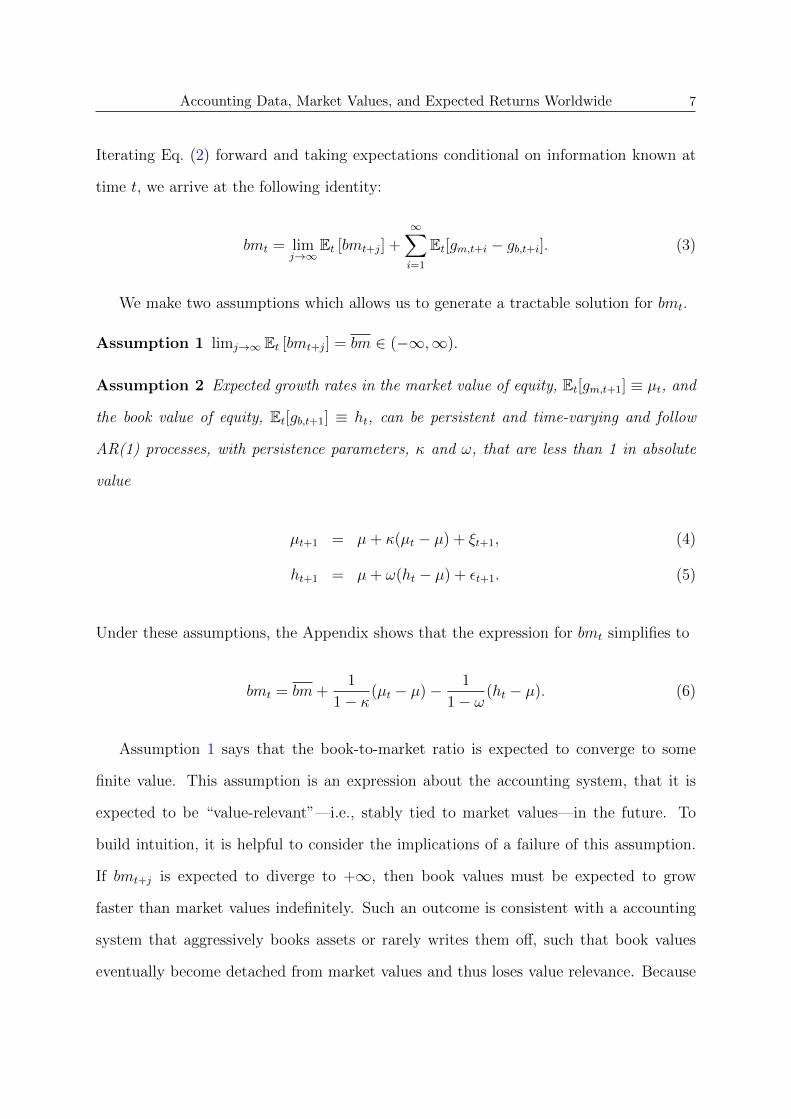
Iterating Eq. (2) forward and taking expectations conditional on information known at
time t, we arrive at the following identity:
bmt = limj→∞
Et [bmt+j] +∞∑i=1
Et[gm,t+i − gb,t+i]. (3)
We make two assumptions which allows us to generate a tractable solution for bmt.
Assumption 1 limj→∞ Et [bmt+j] = bm ∈ (−∞,∞).
Assumption 2 Expected growth rates in the market value of equity, Et[gm,t+1] ≡ µt, and
the book value of equity, Et[gb,t+1] ≡ ht, can be persistent and time-varying and follow
AR(1) processes, with persistence parameters, κ and ω, that are less than 1 in absolute
value
µt+1 = µ+ κ(µt − µ) + ξt+1, (4)
ht+1 = µ+ ω(ht − µ) + εt+1. (5)
Under these assumptions, the Appendix shows that the expression for bmt simplifies to
bmt = bm+1
1− κ(µt − µ)− 1
1− ω(ht − µ). (6)
Assumption 1 says that the book-to-market ratio is expected to converge to some
finite value. This assumption is an expression about the accounting system, that it is
expected to be “value-relevant”—i.e., stably tied to market values—in the future. To
build intuition, it is helpful to consider the implications of a failure of this assumption.
If bmt+j is expected to diverge to +∞, then book values must be expected to grow
faster than market values indefinitely. Such an outcome is consistent with a accounting
system that aggressively books assets or rarely writes them off, such that book values
eventually become detached from market values and thus loses value relevance. Because

Accounting Data, Market Values, and Expected Returns Worldwide 8
accounting regimes around the world tend to be conservative in nature, it is difficult to
envision an accounting system that would imply that investors expect bmt+j to diverge
to +∞.5 Conversely, if bmt+j is expected to diverge to −∞, then market values are
expected to grow faster than book values indefinitely. Such an outcome is consistent
with an accounting system that is extremely conservative in terms of booking assets or
very quickly writing off assets, such that book values become detached from, and become
irrelevant for, market values. Not only is this divergence unlikely, but it is also inconsistent
with the data. For example, Pastor and Veronesi (2003) show that while the market-to-
book ratio does decline on average as firms age, the ratio settles to a stable value above
1.6 To conclude, because assumption 1 implies an accounting system that is neither very
conservative nor very aggressive, we view assumption 1 to be fairly general and applicable
to the various accounting regimes—i.e., variants of GAAP or IFRS—around the world.
Assumption 2 models the stochastic processes governing expected market and book
growth to be AR(1). The parameters κ and ω of equations (4) and (5) represent the
levels of persistence in expected market and book growth, respectively; µ represents the
unconditional mean expected growth rate for both market and book; and the vector of
innovations (ξt+1, εt+1) are IID through time with zero means and a positive semi-definite
covariance matrix.7
Although this second assumption is statistical in nature, it captures empirical reg-
ularities and economic intuition. The AR(1) assumption for expected market growth
captures the possibility, consistent with the growing body of empirical evidence, that ex-
pected returns can be time-varying (e.g., Cochrane, 2011; Ang and Liu, 2004; Fama and
5Under mark-to-market accounting, which may considered an aggressive regime, book values andmarket values are guaranteed to converge by the definition of marking to market.
6See Figure 5 of their paper.7Contemporaneous correlations between the innovation in expected book and market growth are
possible under this assumption. Thus, while innovations in expected market growth are not correlatedover time, i.e., covt(ξt+n, ξt+k) = 0, and the innovations in book growth are not correlated over time,i.e., covt(εt+n, εt+k) = 0, the only restriction on the contemporaneous covariance between innovations inbook and market growth is boundedness, i.e., |covt(εt+k, ξt+k)| <∞.

Accounting Data, Market Values, and Expected Returns Worldwide 9
French, 2002; Jagannathan, McGrattan, and Scherbina, 2001) and persistent (e.g., Fama
and French, 1988; Campbell and Cochrane, 1999; Pastor and Stambaugh, 2009). The
assumption for expected book growth captures the idea that, while firms can experience
periods of unusually high or low profitability, competitive forces drive a tendency for
accounting rates of returns to revert to a steady-state mean (e.g., Beaver, 1970; Penman,
1991; Pastor and Veronesi, 2003; Healy, Serafeim, Srinivasan, and Yu, 2014).
Two additional observations on these assumptions are worth noting. First, the rever-
sion of expected market and book growth to a common mean (µ) is not an additional
assumption to, but rather than an implication of, the “value-relevance” and AR(1) as-
sumptions. Under assumption 1, the identity of Eq. (3) implies that growth rates of book
and market values must be expected to converge,
limT→∞
Et[gm,t+T − gb,t+T ] = 0. (7)
By assumption 2, convergence is only possible if expected growth in market and book
values share a common mean. This implication is consistent with the economic intu-
ition that in the long run abnormal growth in book values should converge to 0 due to
competition (e.g., Ohlson, 1995). Second, under these assumptions and fixed persistence
parameters, bmt is weakly stationary and bm is the unconditional mean of bm. However,
even under the scenario of an ex post change in the persistence parameters, which would
imply a structural break in bmt, the relation of Eq. (6) would continue to hold so long as
the processes remain AR(1) and the “value relevance” assumption is valid.
Overall, the two assumptions that we impose on the identity of Eq. (3) are fairly
general, applicable to a wide range of accounting systems, and is consistent with empirical
data and economic intuition. In untabulated tests we also find empirical support for these
assumptions.8 These assumptions deliver a parsimonious Eq. (6) relating bm to expected
8In a vast majority of the countries in our sample, we find substantial support for the hypothesis
Accounting Data, Market Values, and Expected Returns Worldwide 10
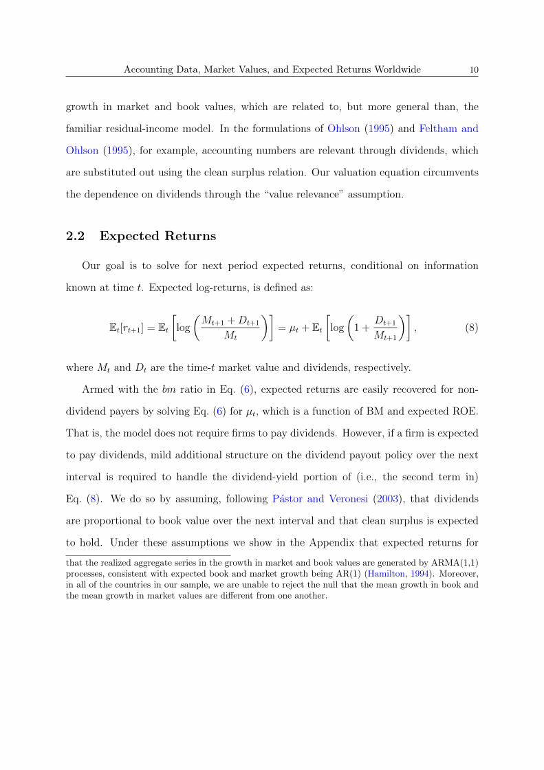
growth in market and book values, which are related to, but more general than, the
familiar residual-income model. In the formulations of Ohlson (1995) and Feltham and
Ohlson (1995), for example, accounting numbers are relevant through dividends, which
are substituted out using the clean surplus relation. Our valuation equation circumvents
the dependence on dividends through the “value relevance” assumption.
2.2 Expected Returns
Our goal is to solve for next period expected returns, conditional on information
known at time t. Expected log-returns, is defined as:
Et[rt+1] = Et[log
(Mt+1 +Dt+1
Mt
)]= µt + Et
[log
(1 +
Dt+1
Mt+1
)], (8)
where Mt and Dt are the time-t market value and dividends, respectively.
Armed with the bm ratio in Eq. (6), expected returns are easily recovered for non-
dividend payers by solving Eq. (6) for µt, which is a function of BM and expected ROE.
That is, the model does not require firms to pay dividends. However, if a firm is expected
to pay dividends, mild additional structure on the dividend payout policy over the next
interval is required to handle the dividend-yield portion of (i.e., the second term in)
Eq. (8). We do so by assuming, following Pastor and Veronesi (2003), that dividends
are proportional to book value over the next interval and that clean surplus is expected
to hold. Under these assumptions we show in the Appendix that expected returns for
that the realized aggregate series in the growth in market and book values are generated by ARMA(1,1)processes, consistent with expected book and market growth being AR(1) (Hamilton, 1994). Moreover,in all of the countries in our sample, we are unable to reject the null that the mean growth in book andthe mean growth in market values are different from one another.

Accounting Data, Market Values, and Expected Returns Worldwide 11
dividend-paying firms is also a linear combination of BM and expected ROE:9
Et[rt+1] = A1 + A2bmt + A3Et[roet+1], (9)
where A1 = K − (1 − κ + ρκ)bm − A3 log(1 + δ) + (κ−ω)(1−ρ)(1−ω) µ, A2 = 1 − κ + ρκ, and
A3 = ρ(κ−ω)+1−κ1−ω ; δ is the proportion of dividends paid out of book; the constants K and
ρ are by-products of a log-linearization around the unconditional bm ratio and close to
zero in value. Thus, even under these rather mild assumptions, as in LW15, expected log
returns can be determined by a constant, bm, and expected roe.10,11
The intuition for why bm and roe provide information on expected returns resides in
the present value relation between prices, expected future payoffs, and expected returns.
Accounting fundamentals provide information on expected future payoffs (cash flows),
while market prices provide information on both expected future payoffs and how they
are discounted. Thus combining market values with accounting numbers, rather than the
latter per se, reveal expected returns.
Consider for illustration the classic Gordon Growth Model, which relates market val-
ues (Mt) to dividends (Dt) as well as constant dividend growth (g) (i.e., expected future
payoffs) and constant expected return (r):
Mt = Dt1 + g
r − g.
9Our assumption of dividends being proportional to book values over one interval, for those expectedto pay dividends, does not imply that dividends are proportional to book for all time. We make thisassumption for tractability and for one-period-ahead returns only. Outside of one-period-ahead returnsfor current dividend-paying firms, we do not rely on dividend-payout policies to generate any of ourresults.
10The interpretation of the coefficients in this paper, however, is slightly different. In LW15, A1 =(ω−κ)k11−ωk1 µ, A2 = 1 − κk1, and A3 = 1−κk1
1−ωk1 , where k1 is a linearization constant assumed to be close toone.
11Under the assumption of constant expected returns, or κ = 0, whereby no growth is expected,expected returns boils down to a function of the earnings-to-price multiple, similar to the approachadvocated by Penman, Reggiani, Richardson, and Tuna (2015).
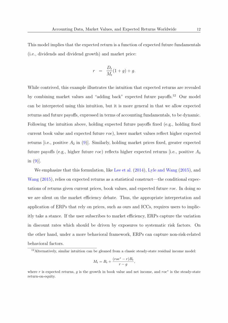
Accounting Data, Market Values, and Expected Returns Worldwide 12
This model implies that the expected return is a function of expected future fundamentals
(i.e., dividends and dividend growth) and market price:
r =Dt
Mt
(1 + g) + g.
While contrived, this example illustrates the intuition that expected returns are revealed
by combining market values and “adding back” expected future payoffs.12 Our model
can be interpreted using this intuition, but it is more general in that we allow expected
returns and future payoffs, expressed in terms of accounting fundamentals, to be dynamic.
Following the intuition above, holding expected future payoffs fixed (e.g., holding fixed
current book value and expected future roe), lower market values reflect higher expected
returns [i.e., positive A2 in (9)]. Similarly, holding market prices fixed, greater expected
future payoffs (e.g., higher future roe) reflects higher expected returns [i.e., positive A3
in (9)].
We emphasize that this formulation, like Lee et al. (2014), Lyle and Wang (2015), and
Wang (2015), relies on expected returns as a statistical construct—the conditional expec-
tations of returns given current prices, book values, and expected future roe. In doing so
we are silent on the market efficiency debate. Thus, the appropriate interpretation and
application of ERPs that rely on prices, such as ours and ICCs, requires users to implic-
itly take a stance. If the user subscribes to market efficiency, ERPs capture the variation
in discount rates which should be driven by exposures to systematic risk factors. On
the other hand, under a more behavioral framework, ERPs can capture non-risk-related
behavioral factors.
12Alternatively, similar intuition can be gleaned from a classic steady-state residual income model:
Mt = Bt +(roe∗ − r)Bt
r − g,
where r is expected returns, g is the growth in book value and net income, and roe∗ is the steady-statereturn-on-equity.
Accounting Data, Market Values, and Expected Returns Worldwide 13
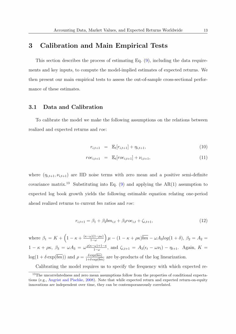
3 Calibration and Main Empirical Tests
This section describes the process of estimating Eq. (9), including the data require-
ments and key inputs, to compute the model-implied estimates of expected returns. We
then present our main empirical tests to assess the out-of-sample cross-sectional perfor-
mance of these estimates.
3.1 Data and Calibration
To calibrate the model we make the following assumptions on the relations between
realized and expected returns and roe:
ri,t+1 = Et[ri,t+1] + ηi,t+1, (10)
roei,t+1 = Et[roei,t+1] + νi,t+1, (11)
where (ηi,t+1, νi,t+1) are IID noise terms with zero mean and a positive semi-definite
covariance matrix.13 Substituting into Eq. (9) and applying the AR(1) assumption to
expected log book growth yields the following estimable equation relating one-period
ahead realized returns to current bm ratios and roe:
ri,t+1 = β1 + β2bmi,t + β3roei,t + ζi,t+1, (12)
where β1 = K +(
1− κ+ (κ−ω)(1−ρω)1−ω
)µ − (1 − κ + ρκ)bm − ωA3log(1 + δ), β2 = A2 =
1 − κ + ρκ, β3 = ωA3 = ω ρ(κ−ω)+1−κ1−ω , and ζi,t+1 = A3(εt − ωνt) − ηt+1. Again, K =
log(1 + δ exp(bm)) and ρ = δ exp(bm)
1+δ exp(bm)are by-products of the log linearization.
Calibrating the model requires us to specify the frequency with which expected re-
13The uncorrelatedness and zero mean assumptions follow from the properties of conditional expecta-tions (e.g., Angrist and Pischke, 2008). Note that while expected return and expected return-on-equityinnovations are independent over time, they can be contemporaneously correlated.

Accounting Data, Market Values, and Expected Returns Worldwide 14
turns and expected roe evolve according to the assumed dynamics. For example, LW15
choose quarterly and annual frequencies. A challenge in the international setting is that
the mandatory frequency of interim reporting is not uniform across markets in different
countries; moreover, some countries changed their mandatory interim financial-reporting
frequency during our sample period (e.g., Link, 2012).
Because annual reporting is required in all countries in our sample, a natural empirical
specification would be to match annual stock returns to annual bm and roe. Given that
fundamental data for most countries become available for a suitable cross section only
between the early and mid-1990s, using annual data imposes serious limitations on the
time series data available to us. The lack of consistency in quarterly reporting across
countries also limits the usefulness of switching to interim reporting.
Our approach to resolving this empirical issue, similar to that of Fama and French
(1992), is to match one-month-ahead returns to annual fundamental data (i.e., matching
one-month-ahead returns to bm and annual roe). This can be thought of as treating
the annual version of Eq. (12) as the sum of 12 equations that contain monthly returns
and news. In this framework, each of the 12 months in a given year is an estimation
equation, using the same BM and annual ROE, and the sum of the 12 estimated monthly
coefficients translates to the coefficients of an annual model. We assume fundamental
data to be known publicly and observable to the researcher four months after the fiscal-
year-end date.14 Thus, in computing a firm’s BM, we use its market capitalization on the
last trading day of the fourth month after the last fiscal-year-ending month.
Our data on returns and fundamentals come from Compustat Global and Compustat
North America (in the case of Canada and the U.S.).15 Monthly returns are computed us-
14This assumption is necessitated by the sparseness of the earnings announcement date variable fora number of countries in Compustat Global. However, among those firms in our sample with earningsannouncement dates, greater than 90 percent of them report annual earnings within four months of thefiscal year end.
15While our use of Compustat for international fundamentals and returns data follows some priorliterature (e.g., Bushman and Piotroski, 2006, Novy-Marx, 2013), the international capital markets

Accounting Data, Market Values, and Expected Returns Worldwide 15
ing Compustat’s price variable (variable prccd from the price file) by applying adjustments
for splits and dividends using the respective adjustment factors (variables ajexdi and trfd
from the price file).16 Gross annual ROE is calculated as ROEi,t =(
1 +Xi,t
Booki,t−1
), where
Xi,t is Net Income before Extraordinary Items (variable ib from the fundamentals file) and
Booki,t−1 is the lag Book Value of Common Equity (variable ceq from the fundamentals
file).
We make forecasts of expected future monthly (log) returns by estimating Eq. (12),
via FM regressions, using historical realized monthly returns, the bm ratio, and roe that
are observable as of the forecast date to avoid look-ahead bias. To ensure stability in the
FM coefficients, we use a training (or burn-in) sample consisting of 40 months in each
country, after which out-of-sample forecasting and testing begins. We use a “cumulative”
window approach, or recursive estimation, in that all historical data available at the time
of the forecast are used to estimate Eq. (12) in order to form expected returns. In other
words, we forecast one-month-ahead expected r at the end of each calendar month by
applying historically-estimated FM coefficients on the bm and roe values observed as of
the forecast date.
Embedded in our country-specific and recursive estimation choices are the implicit
assumptions that 1) expected market growth and expected book growth follow AR(1)
processes with a common long-run mean; 2) these model parameters are country-specific
and may be time-varying; and 3) expected dividend payout ratios are country-specific and
time-varying. The latter assumption differs slightly from LW15, which assumes that the
model parameters are industry-specific. These implementation choices reflect a trade off
between parsimony and realism necessitated by the relative sparsity, both in time series
and cross section, of international equity fundamentals data. In the section on robustness
literature has also used Datastream as a common alternative. Though ex ante we do not expect ourfindings to be influenced by this choice, we re-estimate our main results, in untabulated robustness tests,for a set of major countries using Datastream and find nearly identical results.
16Specifically, log gross returns from t to t+ 1 is computed as log(prccdt+1×trfdt+1
ajexdit+1× ajexdit
prccdt×trfdt
)

Accounting Data, Market Values, and Expected Returns Worldwide 16
tests we describe how relaxing the assumption of constant dividend payouts in the cross
section affects our model parameters.
3.2 Sample Selection
We began with a set of 34 countries whose capital markets and related institutions
have been commonly studied in the international asset pricing literature—Australia, Aus-
tria, Belgium, Canada, China, Denmark, Finland, France, Germany, Greece, Hong Kong,
India, Indonesia, Israel, Italy, Ireland, Japan, Malaysia, Netherlands, New Zealand, Nor-
way, Pakistan, the Philippines, Portugal, Singapore, South Africa, South Korea, Spain,
Sweden, Switzerland, Taiwan, Thailand, the United Kingdom, and the U.S. These include
the 31 countries examined by Leuz et al. (2003) and the 23 countries recognized to have
developed capital markets (e.g., Ang, Hodrick, Xing, and Zhang, 2009; Fama and French,
2012). Because our estimation requires the use of the log of book-to-market multiple and
the log of the gross return-on-equity ratio, firms with negative book values are excluded
from our analyses.
We impose three sets of filters to mitigate the influence of unusual observations on
our estimation and calibration of the paper’s model. First, in each country and on
each forecast date, we eliminate very small and illiquid firms—any firm belonging to
the bottom 2 percent of the cross-section in either market capitalization or liquidity.17
Second, we exclude observations whose stock price belongs to the bottom 5 percent of the
cross-section or is trading below 1 unit of the home currency. Third, to further ensure
the reliability of the cross-sectionally-estimated coefficients, we impose the requirement
that each cross section, after applying the above filters, must have a minimum of 100
observations.
17Following prior research (e.g., LaFond, Lang, and Skaife, 2007), we proxy for a stock’s liquidity usingthe proportion of zero-return days over the prior month. This approximation is necessitated by a lackof a well-populated trading-volume variable in the Compustat Global price files.

Accounting Data, Market Values, and Expected Returns Worldwide 17
These restrictions, in conjunction with a minimum of 40 months of data, eliminate
the following 5 countries from our empirical analyses: Austria, Ireland, New Zealand,
Singapore, and Portugal. Thus, the empirical analyses in our paper examine the efficacy
of our model-implied ERPs for a set of 29 countries worldwide.
We also take measures to ensure that our data are not corrupted by inconsistencies
arising from the use of different currencies to report financial data within a given coun-
try. For the eurozone countries that switched currencies following adoption of the euro,
we convert all pre-adoption financial data to euros using the conversion rate mandated
by the European Central Bank. This translation simply makes the within-country cur-
rency amounts comparable pre- and post-euro conversion. For all other occasions where
companies switch currencies, we drop the two years surrounding the change.18
3.3 Summary Statistics
Table 1 summarizes, by country, our data on the model inputs of Eq. (12). It reports
time-series averages of the distributional statistics of bm and roe. With the exception
of South Korea, all countries on average have (cross-sectional) median bm values that
are negative, a reflection of the tendency for book values to be smaller than market
values. There is wide variation in the central tendency of bm across countries, ranging
from a median bm of 0.11 in South Korea to -1.17 in China. Despite this variation in
central tendency, the spread in the distribution appears similar across most countries. In
contrast, the (time-series) averages of (cross-sectional) median and mean roe values are
relatively uniform across all the countries in our sample.
The last two columns of Table 1 report the initial and final dates for which we have
fundamentals and returns data for each country (after imposing the sample selection
18We set the one-month-ahead returns to missing whenever the given fiscal year’s financials are reportedin a different currency than the following year’s financials. This adjustment affects less than 1% of thesample.

Accounting Data, Market Values, and Expected Returns Worldwide 18
requirements described above). There is some variation in how early the data begins.
For three countries (Canada, Japan, and the U.S.), data became available in the mid- to
late-1980s; for most countries data became available in the early- to mid-1990s. For a
small handful of countries (Belgium, China, Finland, Greece, Israel, Norway, Pakistan,
and the Philippines), data are not available until the 2000s.
Table 2 presents FM coefficients from monthly regressions of one-month-ahead returns
(r) on bm and roe, i.e., the time-series mean of the cross-sectionally-estimated coefficients.
These two accounting-based characteristics explain between 1% and almost 5% of the
cross sectional contemporaneous variation in returns, averaging 2.2%.19 Our findings
suggest that roe exhibits a stronger association with returns compared to bm. The FM
coefficient on roe is positive and significant (at the 10-percent level) in 27 of the 29
countries in our sample; on the other hand, the coefficient on bm is significant (at the
10-percent level) for 21 of the 29 countries.
Finally, we form the model-implied expected one-month-ahead return proxy on each
forecast date using historically-estimated FM coefficients. Recall, at the end of each
calendar month after the initial 40-month burn-in period, we construct a forecast of
one-month-ahead returns by applying the cumulative average of all the cross-sectional
coefficients from estimating Eq. (12) to the currently-available annual bm and roe.
Table 3 reports the time-series average of the cross-sectional distributional summary
statistics for the estimated expected one-month-ahead log returns. We observe substantial
19As noted in Lewellen (2015), FM R2 is not an indicator of predictive power, but reflects the degree towhich the ERP explains contemporaneous variation in returns. To see why, consider the following simpleexample. Suppose that expected returns are constant for all firms (i.e., no cross-sectional variation), butnews has the following structure:
ri,t+1 = er + εi,t+1,
εi,t+1 = Ct+1 × erpi,t,
where Ct+1 is a cross-sectional random variable taking a positive or a negative value with 50% probabilityin a given time period. In this case, even though the proxy (erpi,t) has no predictive ability, in cross-sectional regressions it will completely explain the ex post contemporaneous variation in realized returns,i.e., 100% R2.

Accounting Data, Market Values, and Expected Returns Worldwide 19
within-country variation in the ERP as well as cross-country variation in the (cross-
sectional) mean in the ERP. Comparing the mean expected log return (column 3) to the
mean realized log return (column 10) suggests that our ERPs are on average similar to
future average realized returns for all the countries.20
For ease of interpretation, column (4) reports the mean of expected simple returns
(Ri,t+1) implied by our model-implied ERPs. Based on the standard assumption that
log returns are conditionally normally distributed, expected simple returns can be con-
structed as follows:
Et[Ri,t+1] = exp(µi,t + 0.5× σ2i,t+1), (13)
where µi,t is our expected log return estimate, and σ2i,t+1 is an estimate of the expected
volatility in log returns based on the average squared daily returns from the prior month
scaled by 252/12. Across the 29 countries in our analysis, the cross-sectional mean (me-
dian) monthly expected simple returns is 0.99% (0.91%) or 12.60% (11.43%) annualized.
Though these implied expected simple return estimates are not the main focus of the
paper, we discuss them in more detail later in our robustness tests to assess its relative
performance to factor-based estimates of expected simple returns.
20As can be observed in Table 3, both estimates of expected log returns implied by our model as wellas average realized log returns can be negative, and are always smaller than average simple returns.Because log-returns are a concave function of gross stock returns, by Jensen’s inequality expected log-returns must be weakly less than expected simple stock returns. Moreover, because average monthlysimple returns are low, we can expect average monthly log returns to be negative.
To see these relations more clearly, let gross stock returns, Rt+1, be conditionally log-normally dis-tributed (e.g., van Binsbergen and Koijen, 2010; Bansal and Yaron, 2004; Bansal, Dittmar, and Lundblad,
2005; Black and Scholes, 1973; Campbell, 1993)—i.e., Rt+1 = eqt−12σ
2t+σtεt+1 , where σ2
t represents condi-tional expected stock return variance and εt+1 ∼ N(0, 1). Under this structure, expected simple rates ofreturn are given by qt, or Et[Rt+1] = eqt . Taking logs of gross returns and then expectations, we obtainEt[log(Rt+1)] ≡ µt = qt − 1
2σ2t . Therefore, when average monthly returns are relatively small—i.e.,
qt <12σ
2t—then expected log-returns can be negative.

Accounting Data, Market Values, and Expected Returns Worldwide 20
3.4 Cross-Sectional Validation Tests
We next turn to validating the model-implied ERPs and assessing their reliability
across worldwide markets. We first examine how the proxies, on average, are associated
with future returns. We then assess performance against standard factor-model-based
proxies.
3.4.1 Regression Based Tests
Our primary test for assessing the reliability of our ERPs is the standard regression-
based test as employed by, for example, Lewellen (2015) and Lyle and Wang (2015). In
particular, we separately estimate for each country cross-sectional predictive regressions
of 1-month-ahead r on our ERPs:
ri,t+1 = δ0 + δ1Et[ri,t+1] + wi,t+1. (14)
A perfect proxy of expected returns implies δ0 = 0 and δ1 = 1. In particular, having a
slope coefficient close to 1 suggests that the magnitudes of the cross-sectional differences
in the ERP are informative of the magnitude of differences in expected returns, which
facilitate inferences in regression settings. More generally, positive and significant δ1
coefficients imply positive return sorting ability on average. To reduce the influence of
unusually large values in our estimates, we winsorize the expected return measures at the
top and bottom 1 percent.
Table 4 reports FM regression estimates of Eq. (14) for the 29 countries in the sample.
The results in this table indicate that the model-implied ERPs strongly and significantly
predict realized returns for a vast majority of the countries. Coefficients on expected
returns (the “predictive slope coefficient”) are statistically significant at the 5-percent
and 10-percent levels for 24 and 26 of the 29 countries, respectively. Greece, Pakistan,

Accounting Data, Market Values, and Expected Returns Worldwide 21
and South Africa’s predictive slope coefficients do not differ significantly from 0 at the
10% level; in the case of Pakistan, the slope is also indistinguishable from 1.
The average slope coefficient across the 29 countries is 1.05. Based on the F-test for
the null hypothesis that the slope is equal to 1 (reported in the last row of Table 4),
we reject the null for only 9 (10) of the 29 countries at the 10-percent (5-percent) level.
Furthermore, we fail to reject the null that the constant term is equal to 0 at the 5-percent
level for all but 2 countries in our sample. In the aggregate, these regression-based test
results suggest that our accounting-based ERPs line up well with expected returns and are
reliably associated with the cross section of future returns across international markets.21
3.4.2 Portfolio Sort Tests
We supplement the above parametric return regression tests with portfolio-level anal-
ysis. To conduct these non-parametric tests, we construct equal-weighted portfolios at
the end of each calendar month based on the quintile rankings of the ex ante ERP, and
summarize the average 1-month-ahead returns realized by each portfolio. Our choice of
quintile portfolios is intended to ensure that, for any given country on any given month,
there are at least 20 stocks in each portfolio.
Table 5 provides further evidence that, consistent with the regression tests of Table
4, the model-implied proxies exhibit significant ability to predict the cross-section of
future returns. We document in column (6) significant average spreads between the top
and bottom quintile portfolios for 24 countries. Though these results are statistically
slightly weaker, they are broadly consistent with the regression-based tests. In fact, the
portfolio sorts are robust enough that for the majority of the countries (20), even the
spread between the portfolio median returns, reported in column (7), are statistically
significant.
21In untabulated robustness tests, we find that winsorizing the inputs at the top and bottom 1 percentof each cross section yields ERPs that produce virtually identical results.
Accounting Data, Market Values, and Expected Returns Worldwide 22
Collectively, these results imply that reliable firm-level expected stock returns that
are applicable to worldwide markets can be constructed with a linear combination of bm
and roe. These findings also demonstrate, consistent with Lewellen (2015), that firm-level
ERPs obtained from FM regressions exhibit strong cross-sectional predictive properties.
3.5 Robustness Tests
In this section we assess the performance of factor-model-based ERPs to contextualize
our main findings. We also describe how relaxing the assumption of dividend payouts
being constant in the cross section affects our model parameters. Finally, we discuss
untabulated analyses on the sensitivity of the ERPs to variations in the training sample
period as well as performance based on alternative evaluative frameworks.
3.5.1 Factor-Based Estimates
To contextualize our main empirical results, we assess the performance of firm-level
ERPs derived from the global and regional four-factor models described in Fama and
French (2012). These are global and regional versions of the Fama and French (1993)
three-factor model augmented with the momentum factor, but the factor returns are based
on portfolios that encompass 23 countries in four regions: Australia, Austria, Belgium,
Canada, Denmark, Finland, France, Germany, Greece, Hong Kong, Ireland, Italy, Japan,
the Netherlands, New Zealand, Norway, Portugal, Singapore, Spain, Switzerland, Sweden,
U.K., and U.S. We obtain monthly global and regional factor returns from Ken French’s
data library.22
At the end of each calendar month (t), one-month-ahead factor-based ERPs for a firm
22http://mba.tuck.dartmouth.edu/pages/faculty/ken.french/data_library.html

Accounting Data, Market Values, and Expected Returns Worldwide 23
(i) are constructed as follows:
Et[ri,t+1] = rft+1 + γi,RMRF Et[RMRFt+1] + γi,SMBEt[SMBt+1] (15)
+γi,HMLEt[HMLt+1] + γi,WMLEt[WMLt+1].
Here Et[RMRFt+1], Et[SMBt+1], Et[HMLt+1], and Et[WMLt+1] represent the expected
global or regional market, size, value, and momentum factor returns, respectively, which
we estimate based on the trailing average 40-month realized factor returns. γi,j represents
the factor j loadings for a firm, estimated in time-series for each firm i using monthly
stock and factor returns over the 40 months prior to the forecast date. Risk-free rates are
proxied by U.S. treasury yields. Because the global and regional factors are calculated
using US-Dollar-denominated returns, for consistency in this exercise we convert all price
series to U.S. Dollars and compute U.S.-Dollar-denominated returns for all firms in our
sample.
Because these factor-based models yield expected simple returns, we compare them
against our model-implied estimate of expected simple returns following Eq. (13). Table
6 reports the results of regression-based tests for the global- and regional-factor-based
ERPs for the 29 countries in our sample alongside the results of the model-implied simple
ERPs. To facilitate comparisons, we use a common set of firm-year observations for
which all three ERPs are available. Like our results in Table 4, the model-implied simple
ERPs perform very well across all 29 countries. In fact, the predictive slope coefficient
is positive and significant for all 29 countries. In striking contrast, with the exception
of one country, the global- and regional-factor-based ERPs do not exhibit out-of-sample
return predictability. The exception is in Pakistan, for which the global four-factor model
exhibits a modest slope coefficient of 0.2548 that is significant at the 10% level. For the
remaining countries the slope coefficients are either significantly negative (4 countries) or

Accounting Data, Market Values, and Expected Returns Worldwide 24
indistinguishable from zero at the 10-percent level.
We also consider the recent Fama and French (2014) five-factor model, which augments
Fama and French (1993)’s original three-factor model with a profitability factor and
an investment factor. Fama and French (2014) show that this expanded model better
explains the cross section of average returns in-sample compared to the three-factor
model, similar to the conclusions of Hou, Xue, and Zhang (2014). We complement these
findings by assessing the out-of-sample performance of five-factor-based ERPs, reported
in the second-to-last row of Table 6. Our regression-based tests of this model are restricted
to the U.S. since profitability and investment factor returns are not available globally. As
with the four-factor model, we find that this expanded model does not produce ERPs that
are robustly associated with future returns. We document a negative but insignificant
slope coefficient.
Finally, we consider a variation of the new factor model that incorporates only the
market, value, and profitability factors, representing a close factor-based counterpart to
our paper’s characteristic-based model. The out-of-sample performance, reported in the
last row of Table 6, continues to be poor, as the proxy exhibits a negative and significant
slope coefficient at the 10-percent level.
Juxtaposed against the performance of our model-implied simple ERPs, these results
overall show that the out-of-sample cross-sectional predictive ability of our model-implied
ERPs dramatically outperform that of alternative factors-based proxies. We note that
these findings need not necessarily invalidate the factor models per se, but could be con-
sistent with the possibility that firm characteristics better capture time-varying factor
loadings and premiums (e.g., Cochrane, 2011), which are notoriously difficult to estimate
(Fama and French, 1997). This evidence is also consistent with and generalizes the find-
ings of LW15 across international markets and accounting systems, broadly echoing the
views of Campbell, Polk, and Vuolteenaho (2010) that accounting information is useful in

Accounting Data, Market Values, and Expected Returns Worldwide 25
explaining firm level expected rate of returns. More strongly, our evidence suggest that
accounting-based valuation models provide a unifying framework for estimating firm-level
expected rates of returns around the world.
3.5.2 Dividend Payout Variation
To help validate the assumptions used in the model we analytically and empirically
examine how the coefficients A2 and A3 embedded in (12) depend on the dividend payout
ratio. We show in the Appendix that the loading on bm and roe is expected to increase
with the payout ratio.23 We test these formal predictions empirically by estimating the
following contemporaneous Fama-MacBeth regression:
ri,t+1 = β1 + β2 × bmi,t + β3 × roei,t+1 + β4 × payouti,t+1 (16)
+β5 × bmi,t × payouti,t+1 + β6 × roei,t+1 × payouti,t+1 + ζi,t+1,
where payouti,t+1 = Dividendsi,t+1/Booki,t+1, which is consistent with the model pre-
sented in the paper. The empirical results, reported in Table 7, largely support the
theoretical predictions. The coefficients on the interactions of bm and roe with payout
are positive and statistically significant in a large number of countries. Specifically, the
coefficient on bm×payout is positive in all but one country in our sample, and is statisti-
cally significant at the 10-percent level in 23 countries. The coefficient on roe× payout is
positive for all but two countries; however, the statistical significance of this coefficient is
less strong, with 14 being significant at the 10-percent level. We note that the statistical
significance of these results are likely in part attenuated by noise in the dividend data.
Our discussions with the S&P revealed that there is a variation in the accuracy with
23This is true so long as the persistence of expected returns is positive and is greater than the per-sistence of expected profitability, i.e., κ > ω. Indeed, the average coefficients on bm and roe acrosscountries implies persistence parameters of κ ≈ 0.98 and ω ≈ 0.88, values that are consistent with thosedocumented in Lyle and Wang (2015).

Accounting Data, Market Values, and Expected Returns Worldwide 26
which Compustat Global captures dividends across countries. Nevertheless, these esti-
mates are broadly consistent with the model’s predictions that firms with higher future
payouts should produce higher loadings on the accounting-based characteristics.
3.5.3 Sensitivity to Training Sample Window
In untabulated tests we also assess the sensitivity of our proxies to the choice of the
burn-in period. Our baseline results use the first 40 months of data as the training sample
before constructing ERPs and conducting out-of-sample tests. Our choice of 40 months,
which we view to be a relatively short training period, was motivated by the relatively
short sample of available data in certain countries (e.g., Israel and Pakistan).
We vary the training window to include 30 and 50 months and, for nearly all coun-
tries, these variations in the training sample period do not affect our inferences. For
Finland and the Netherlands, widening the training sample and reducing the testing
window reduces the statistical significance slightly, with t-statistics of 1.56 and 1.33, re-
spectively. Reducing the training window to 30 months marginally affects one country—
Switzerland—whose predictive coefficient remains positive and large in magnitude with a
borderline t-statistic of 1.63. Overall, however, our main findings on the association with
the cross section of future returns across countries are not very sensitive to the training
window period.
3.5.4 Association with Risk Proxies
As we discussed in the Introduction, this paper focuses on expected returns as a
statistical construct, and in doing so we cannot offer insight into the market efficiency
debate. Thus interpretation and use of proxies like ours, that depend on market prices,
necessitates taking a stance. If one subscribes to market efficiency, expected returns
should only be a function of sensitivities or exposures to risk factors. Conversely, in a

Accounting Data, Market Values, and Expected Returns Worldwide 27
behavioral framework, expected returns can also be a function of other non-risk-related
behavioral factors.
However, in unreported tests, we find that our expected simple return proxies are
significantly associated with traditional measures of risk. In particular, we find positive
and significant associations (at the 1% level) with market beta and log book-to-market,
and negative and significant associations (at the 1% level) with size (i.e., log of market
capitalization) and liquidity (i.e., percent of zero-return days over the prior month). Note
that while the correlation with book-to-market is not surprising, its inclusion ensures that
the correlation with alternative risk proxies are not driven by it. The positive association
with market beta is also notable, suggesting that the noisiness in estimating factor risk
premiums plays an important role in the poor performance of factor-based ERPs. These
findings overall suggest that our model-implied ERPs are also validated based on the
alternative evaluative framework that is adopted in the literature (e.g., Botosan et al.,
2011), i.e., based on ERPs’ associations with commonly-accepted risk proxies.
4 Accounting Quality: Implications and Tests
While the empirical evidence presented above establishes the usefulness of accounting
information in estimating expected returns across the world, accounting systems, and
the quality of the information they produce, can significantly vary from one market and
institutional setting to another. This section analyzes, both analytically and empirically,
how our model of expected returns is affected by the quality of accounting information
provided to investors.

Accounting Data, Market Values, and Expected Returns Worldwide 28
4.1 Model Setup and Key Implication
To investigate this issue analytically, we extend the baseline model of expected returns
to a setting where information is imperfect. To introduce the concept of imperfections
in the accounting system vis-a-vis return prediction, we assume that investors do not
directly observe expected growth in book value, ht, but learn about it dynamically over
time using realized accounting reports.24
In the spirit of Dechow, Ge, and Schrand (2010), we assume that investors observe
financial reports of book growth, gb,t+1, which reflects both “true” firm performance
(gtrue,t+1) and noise (ξrt+1) from the accounting system:
gb,t+1 = gtrue,t+1 + ξrt+1, and (17)
gtrue,t+1 = ht + ξtruet+1 . (18)
It follows that observed reports of book growth (gb,t+1) have two sources of noise: (1)
true “fundamental” or “innate” noise (ξtruet+1 ) and (2) measurement errors from the ac-
counting system (ξrt+1). We assume that the noise in the reports is captured by two
independent error terms, ξtruet+1 ∼ N(0, σ2) and ξrt+1 ∼ N(0, σ2r).
25 Mapping this back into
the assumptions about growth in book value (5), we have:
gb,t+1 = ht + ξtruet+1 + ξrt+1. (19)
Since investors observe only realized growth in book values, they form expectations
of book growth by making inferences (or learning) about the unobserved ht using rele-
24Unlike related studies in the literature (e.g., van Binsbergen and Koijen, 2010), we do not assumethat investors need to filter expected returns. Our rationale is that since investors set prices, given theirexpectations of book growth they must also set expected market returns. Our setting is thus closelyrelated to that of Pastor and Veronesi (2003, 2006), except that we do not assume an exogenous discountfactor.
25While the assumption of Gaussian error terms is common and somewhat restrictive, the assumptionof independence is without loss of generality.

Accounting Data, Market Values, and Expected Returns Worldwide 29
vant information to optimally update their beliefs over time. We denote ft = E[ht|Ft]
as investors’ beliefs about mean book growth given Ft, where Ft = {gb,τ}τ∈{0,1,...,t} rep-
resents the history of accounting reports available to investors. Assuming that ht is also
conditionally Gaussian, it can be shown that investors’ optimal dynamic updates to their
beliefs take the following form:
f t+1 = µ+ ω(ft − µ) +ωvt
σ2 + σ2r + vt
(gb,t+1 − ft), (20)
where vt = E[(ft−E[ft|Ft])2|Ft] is the conditional variance of ft with respect to investors
filtration Ft, or the dispersion in investors’ prior beliefs; σ2h is the conditional variance of
ht; and vt+1 = ω2vt + σ2h −
ω2v2tσ2+σ2
r+vt.26
Using this updating rule, we show in the Appendix that when the accounting system
is imperfect, expected stock returns are a linear combination of bm and roe:
E[rt+1|Ft] = C1(t) + C2(t)ft−1 + C3bmt + C4(t)roet, (21)
in which the coefficient on roe takes the following form
C4(t) = A3ωvt−1
σ2 + σ2r + vt−1
. (22)
This model provides the key insight that, all else equal, better accounting informa-
tion quality elevates the importance of roe in forecasting future returns. Specifically,
conditional on the dispersion of investors’ prior beliefs (vt−1), the volatility in the under-
lying fundamentals (σ2), and the persistence in expected returns and expected roe, the
coefficient on roe is increasing with accounting information quality (or decreasing in σ2r).
The above analytical approach also allows a reconciliation of our model to the various
26This follows directly from Theorem 13.4 of Liptser and Shiryaev (1977).

Accounting Data, Market Values, and Expected Returns Worldwide 30
alternative firm characteristics and signals (e.g., valuation ratios and accounting data)
that relate to future stock returns. In particular, generalizing the above to include mul-
tiple information sources in investors’ information set, if a signal systematically forecasts
future payoffs (i.e., future roe), conditional on bm, it follows that such a variable is also
systematically associated with expected returns. This insight suggests that the empirical
approach used by Ou and Penman (1989), coupled with our parsimonious model, may
offer an exciting area of potential future research in accounting and characteristic-based
asset pricing.
4.2 Empirical Tests
We proceed to empirically test the prediction that, all else equal, higher-quality ac-
counting information leads investors to place greater weight on roe in inferring expected
returns. Accounting information quality, specifically the variance in measurement errors
in the context of the model above, is difficult to measure. Under the view that greater
variation in information quality exist across (rather than within) countries, our empirical
approach exploits cross-country variation in the data. To do so, we adopt the methodol-
ogy of Leuz et al. (2003) which creates a composite country-level measure of accounting
quality by averaging a given country’s rankings across four dimensions.
The first two dimensions of information quality capture the extent to which firms in
a given country engage in earnings smoothing. The first earnings-smoothing measure
(Variability) takes each country’s median ratio of firm-level standard deviation of oper-
ating earnings divided by the firm-level standard deviation of cash-flow from operations,
and ranks these median ratios across countries in descending order. A lower ratio implies
a greater degree of earnings smoothing, and hence lower earnings quality, resulting in a
higher rank. The second earnings-smoothing measure (Correlation) takes the magnitude
of the contemporaneous correlation between changes in accounting accruals and changes

Accounting Data, Market Values, and Expected Returns Worldwide 31
in operating cash flows in each country, and ranks this correlation across countries in
ascending order. This correlation is estimated by pooling all firm-years within a coun-
try; a greater magnitude implies greater earnings smoothing and lower earnings quality,
resulting in a higher rank.
The third and fourth dimensions of information quality measures the extent of the
use of accruals to manage earnings in a given country. The third measure (Accruals
Magnitude) takes the median of the ratio between the absolute value of firm accruals and
the absolute value of firm cash-flow from operations in a given country, and ranks this
measure across countries in ascending order. A higher median ratio implies a greater use
of accruals to manage earnings, and lower earnings quality, resulting in a higher rank. The
fourth and final dimension of poor information quality (Small Loss Avoidance) takes the
ratio between instances of small profits and instances of small losses, calculated by pooling
all firm-years within a country, and ranks the measure across countries in ascending order.
Small profits and small losses are calculated using earnings scaled by total assets, where
small losses are defined as in the range [−0.01, 0) and small profits are defined as in the
range [0.00, 0.01]. A higher ratio implies greater use of managerial discretion in managing
earnings, and lower earnings quality, resulting in a higher rank.
Our main empirical test, reported in Table 8, exploits the cross-country variations
between this proxy, Poor Information Quality, and the median roe coefficient, generated
from monthly regressions of Eq. (12). That is, we assess the cross-country relation be-
tween the the average level of information quality and the average importance of roe in
forecasting returns over the relevant time frame.27
Column (1) of the table reports OLS estimates of regressions of each country’s median
roe coefficient on its Poor Information Quality measure and a control for the size of
27This approach is consistent with, but need not depend on, the assumption that earnings quality ina country is constant through time.

Accounting Data, Market Values, and Expected Returns Worldwide 32
each country’s equity market.28 The rationale for such a control is to address the “all
else equal” aspect of the theoretical predictions. Holding accounting information quality
constant, the presence of more of information intermediaries may reduce the importance of
roe. Consistent with this intuition, our result shows a negative and significant coefficient
on market size. Moreover, consistent with the model predictions, we report a negative
coefficient on Poor Information Quality, but it is not statistically significant.29
We interpret the lack of significance in Poor Information Quality as, at least in
part, a result of errors in measuring countries’ accounting systems’ measurement error
variances—the underlying theoretical variable of interest—which is consistent with the
coefficient’s attenuation to 0. We resolve this issue empirically by using an instrumental-
variables approach to identify the effect of information quality on the importance of roe.
Our instruments capture the quality of governance institutions in a given country. Our
identifying assumption is that the strength of such institutions affects the importance of
roe in forecasting future returns only by improving the information quality produced
by firms in equity markets. Our instrument, Quality of Governance Institutions, is con-
structed using data from the World Bank’s Worldwide Governance Indicators project,
which compiles five metrics on countries’ governance institutions.30 Rule of Law cap-
tures perceptions of the quality of contract enforcement, property rights, and the courts;
Accountability captures perceptions of the extent to which citizens have the ability to
exert their voices and influence to create accountability in society, including freedom to
select their government and the presence of a free media; Political Stability measures
perceptions of the likelihood of political instability; Government Effectiveness captures
perceptions of the quality of public services and the robustness of the policy formulation
28Specifically, we take the log of the median total market capitalization over the relevant time framefor a given country.
29These results exclude Greece, Pakistan, and South Africa, for which the model does not generatereliable proxies. Taiwan is also excluded because information on the strength and quality of its governanceinstitutions is unavailable.
30http://info.worldbank.org/governance/wgi/index.aspx#home

Accounting Data, Market Values, and Expected Returns Worldwide 33
process; and Control of Corruption captures perceptions of the extent to which public
power is exercised for private benefits. We take the median value of each variable over the
relevant time frame for each country and then standardize each measure using the cross-
section of countries. Our final country-level variable, Quality of Governance Institutions,
is the simple average of the five standardized governance measures.
Columns (2) and (3) report the first- and second-stage results, respectively, of an
instrumental-variables estimation in which we instrument Poor Information Quality with
Quality of Governance Institutions. The first-stage estimation results suggest that higher-
quality or stronger governance institutions in a country are significantly associated (at the
1% level) with higher-quality accounting information, consistent with economic intuition.
In the second stage we find that, all else equal, better earnings quality increases the im-
portance of roe in forecasting returns. Specifically, improving a country’s earnings-quality
rank by 1 unit increases the roe coefficient by about 0.001, representing an economically
significant increase of approximately 10 percent for the median country. Consistent with
measurement errors influencing the OLS results, the magnitude of the coefficient in the
instrumental-variables specifications is substantially larger compared to the baseline OLS
specification. Finally, the last column of the table reports the reduced-form OLS estimates
from regressing the median roe coefficients on the governance-quality variable and the
market size control. Consistent with our instrumental-variables estimates, these results
show that stronger and higher-quality governance institutions elevate the importance of
roe in forecasting returns.
Table 9 provides further analyses of the impact of information quality on the roe coeffi-
cient by examining the four different dimensions of Poor Information Quality separately.
All four measures produce negative coefficients, and all but Variability are significant
at the 10% level. Accruals Magnitude yields the strongest results, with statistical sig-
nificance at the 5% level. Together with Table 8, these findings as consistent with the

Accounting Data, Market Values, and Expected Returns Worldwide 34
analytical prediction that roe plays a reduced role in forecasting returns when accounting
information quality is lower.
5 Conclusion
We show that, under fairly general assumptions, expected returns is related to bm
and roe. This parsimonious linear relation is not only theoretically applicable to various
accounting systems, but also supported empirically: the model-implied ERPs predict the
cross section of future returns and line up well with expected returns across international
markets. Our work promotes an accounting-based approach to expected returns, and
contributes to the stream of empirical studies devoted to developing the estimation of,
and understanding the behavior of, expected returns. It also provides a practical tool
that can be used to analyze investment choices in international equity contexts.
This tractable model not only performs well empirically but can easily incorporate
and generate analytical predictions that are not possible in traditional factor-based or
ICC models. In particular, our analytical work in integrating the model of expected
returns to a dynamic information setting allows for an analysis of how characteristics of
accounting systems—specifically the quality of accounting information produced—affects
the inference of expected returns.
Although our model produces proxies consistent with expected returns, it does not
allow us to distinguish whether prices are efficient or to rationalize whether, or how,
the combination of bm and roe are related to systematic versus unsystematic risk. Such
an endeavor would require further theoretical investigation, which would be fruitful for
future research. Future work could also examine how valuation models like ours, based
on “traditional” accounting variables (e.g., book values and ROE), are connected to the
investment-based models that have been more recently proposed (e.g., Liu, Whited, and

Accounting Data, Market Values, and Expected Returns Worldwide 35
Zhang, 2009; Belo, Xue, and Zhang, 2013; Hou et al., 2014). Finally, although this paper
anchors market values of equity to book values of equity, which we believe to be a natural
choice, it is possible to derive expected returns as a function of alternative multiples and
ratios using the structure laid out in this paper. We believe that developing a theory for
the appropriate use of the various valuation multiples and performance ratios observed
in practice would be an important area of future work.

Accounting Data, Market Values, and Expected Returns Worldwide 36
References
Ang, A., R. J. Hodrick, Y. Xing, and X. Zhang (2009). High idiosyncratic volatilityand low returns: International and further U.S. evidence. Journal of Financial Eco-nomics 91 (1), 1–23.
Ang, A. and J. Liu (2004). How to discount cashflows with time-varying expected returns.Journal of Finance 59 (6), 2745–2783.
Angrist, J. D. and J. Pischke (2008). Mostly harmless econometrics: An empiricist’scompanion. New Jersey: Princeton University Press.
Bansal, R., R. Dittmar, and C. Lundblad (2005). Consumption, dividends, and the crosssection of equity returns. Journal of Finance 60 (4), 1639–1672.
Bansal, R. and A. Yaron (2004). Risks for the long run: A potential resolution of assetpricing puzzles. Journal of Finance 59 (4), 1481–1509.
Beaver, W. H. (1970). The Time Series Behavior of Earnings. Journal of AccountingResearch 8 (May), 62–99.
Belo, F., C. Xue, and L. Zhang (2013). A supply approach to valuation. Review ofFinancial Studies 26 (12), 3029–3067.
Black, F. and M. Scholes (1973). The pricing of options and corporate liabilities. TheJournal of Political Economy , 637–654.
Botosan, C. (1997). Disclosure level and the cost of equity capital. The AccountingReview 72 (3), 323–349.
Botosan, C. and M. Plumlee (2005). Assessing alternative proxies for the expected riskpremium. The Accounting Review 80 (1), 21–53.
Botosan, C., M. Plumlee, and H. Wen (2011). The relation between expected returns, re-alized returns, and firm risk characteristics. Contemporary Accounting Research 28 (4),1085–1122.
Bushman, R. M. and J. D. Piotroski (2006). Financial reporting incentives for conserva-tive accounting: The influence of legal and political institutions. Journal of Accountingand Economics 42 (1), 107–148.
Campbell, J. (1993). Intertemporal asset pricing without consumption data. The Amer-ican Economic Review 83 (3), 487–512.
Campbell, J. Y. and J. H. Cochrane (1999). By force of habit: A consumption-basedexplanation of aggregate stock market behavior. The Journal of Political Econ-omy 107 (2), 205–251.
Accounting Data, Market Values, and Expected Returns Worldwide 37
Campbell, J. Y., C. Polk, and T. Vuolteenaho (2010). Growth or glamour? Fundamentalsand systematic risk in stock returns. Review of Financial Studies , 305–344.
Chen, H., J. Z. Chen, G. J. Lobo, and Y. Wang (2011). Effects of audit quality onearnings management and cost of equity capital: Evidence from China. ContemporaryAccounting Research 28 (3), 892–925.
Claus, J. and J. Thomas (2001). Equity premia as low as three percent? evidence fromanalysts’ earnings forecasts from domestic and international stock markets. Journal ofFinance 56 (5), 1629 – 1666.
Cochrane, J. (2011). Presidential address: Discount rates. Journal of Finance 66 (4),1047–1108.
Dechow, P., W. Ge, and C. Schrand (2010, December). Understanding earnings quality: Areview of the proxies, their determinants and their consequences. Journal of Accountingand Economics 50 (2-3), 344–401.
Easton, P. and S. Monahan (2005). An evaluation of accounting-based measures ofexpected returns. The Accounting Review 80 (2), 501.
Easton, P. D. (2004). Pe ratios, peg ratios, and estimating the implied expected rate ofreturn on equity capital. The Accounting Review 79, 73 – 96.
Fama, E. and K. French (1992). The cross-section of expected stock returns. The Journalof Finance 47 (2), 427–465.
Fama, E. and K. French (1997). Industry costs of equity. Journal of Financial Eco-nomics 43 (2), 153–193.
Fama, E. F. and K. R. French (1988). Dividend yields and expected stock returns. Journalof financial economics 22 (1), 3–25.
Fama, E. F. and K. R. French (1993). Common risk factors in the returns on stocks andbonds. Journal of financial economics 33 (1), 3–56.
Fama, E. F. and K. R. French (2002). The equity premium. The Journal of Finance 57 (2),637–659.
Fama, E. F. and K. R. French (2012). Size, value, and momentum in international stockreturns. Journal of Financial Economics 105 (3), 457–472.
Fama, E. F. and K. R. French (2014). A five-factor asset pricing model. Journal ofFinancial Economics .
Fama, E. F. and J. D. MacBeth (1973). Risk, return, and equilibrium: Empirical tests.The Journal of Political Economy , 607–636.

Accounting Data, Market Values, and Expected Returns Worldwide 38
Feltham, G. A. and J. A. Ohlson (1995). Valuation and clean surplus accounting foroperating and financial activities. Contemporary Accounting Research 11 (2), 689–731.
Gebhardt, W. R., C. M. C. Lee, and B. Swaminathan (2001). Toward an implied cost ofcapital. Journal of Accounting Research 39 (1), 135–176.
Gode, D. and P. Mohanram (2003). Inferring the cost of capital using the Ohlson–Juettnermodel. Review of Accounting Studies 8 (4), 399–431.
Green, J., J. R. M. Hand, and X. F. Zhang (2013). The supraview of return predictivesignals. Rev. Account. Stud. 18 (3), 692–730.
Hail, L. and C. Leuz (2006, June). International differences in the cost of equity cap-ital: Do legal institutions and securities regulation matter? Journal of AccountingResearch 44 (3), 485–531.
Hamilton, J. D. (1994). Time Series Analysis. New Jersey: Prentice Hall.
Haugen, R. A. and N. L. Baker (1996). Commonality in the determinants of expectedstock returns. Journal of Financial Economics 41 (3), 401–439.
Healy, P., G. Serafeim, S. Srinivasan, and G. Yu (2014). Market competition, earningsmanagement, and persistence in accounting profitability around the world. Review ofAccounting Studies 19 (4), 1–28.
Hou, K., G. A. Karolyi, and B.-C. Kho (2011). What factors drive global stock returns?Review of Financial Studies 24 (8), 2527–2574.
Hou, K., C. Xue, and L. Zhang (2014). Digesting anomalies: An investment approach.Review of Financial Studies , 650–705.
Jagannathan, R., E. R. McGrattan, and A. Scherbina (2001). The declining us equitypremium. Technical report, National Bureau of Economic Research.
LaFond, R., M. Lang, and H. A. Skaife (2007). Earnings smoothing, governance and liq-uidity: international evidence. Massachusetts Institute of Technology Working Paper .
Lambert, R., C. Leuz, and R. E. Verrecchia (2007). Accounting information, disclosure,and the cost of capital. Journal of Accounting Research 45 (2), 385–420.
Lee, C., D. Ng, and B. Swaminathan (2009). Testing international asset pricing modelsusing implied costs of capital. Journal of Financial and Quantitative Analysis 44 (2),307.
Lee, C., E. So, and C. C. Wang (2014). Evaluating implied cost of capital estimates.Stanford University Working Paper .

Accounting Data, Market Values, and Expected Returns Worldwide 39
Leuz, C., D. Nanda, and P. D. Wysocki (2003). Earnings management and investorprotection: an international comparison. Journal of Financial Economics 69 (3), 505–527.
Lewellen, J. (2015). The cross section of expected stock returns. Forthcoming in CriticalFinance Review .
Link, B. (2012). The struggle for a common interim reporting frequency regime in Europe.Accounting in Europe 9 (2), 191–226.
Liptser, R. and A. Shiryaev (1977). Statistics of random processes: Applications, Vol-ume 2. Springer Verlag.
Liu, L. X., T. M. Whited, and L. Zhang (2009). Investment-based expected stock returns.Journal of Political Economy 117 (6), 1105–1139.
Lyle, M. R., J. L. Callen, and R. J. Elliott (2013). Dynamic risk, accounting-basedvaluation and firm fundamentals. Review of Accounting Studies 18 (4), 899–929.
Lyle, M. R. and C. C. Wang (2015). The cross section of expected holding period returnsand their dynamics: A present value approach. Journal of Financial Economics 16 (3),505–525.
Novy-Marx, R. (2013). The other side of value: The gross profitability premium. Journalof Financial Economics 108 (1), 1–28.
Ohlson, J. (1995). Earnings, book values, and dividends in equity valuation. Contempo-rary Accounting Research 11 (2), 661–687.
Ou, J. A. and S. H. Penman (1989). Financial statement analysis and the prediction ofstock returns. Journal of Accounting and Economics 11 (4), 295–329.
Pastor, L. and R. F. Stambaugh (2009). Predictive systems: Living with imperfectpredictors. The Journal of Finance 64 (4), 1583–1628.
Pastor, L. and P. Veronesi (2003). Stock valuation and learning about profitability.Journal of Finance 58 (5), 1749–1790.
Pastor, L. and P. Veronesi (2006). Was there a Nasdaq bubble in the late 1990s? Journalof Financial Economics 81 (1), 61–100.
Pastor, L. and P. Veronesi (2009). Learning in financial markets. Annual Review ofFinancial Economics 1 (1), 361–381.
Penman, S., F. Reggiani, S. Richardson, and I. Tuna (2015). A characteristic model forasset pricing and risky value slides. Working Paper .

Accounting Data, Market Values, and Expected Returns Worldwide 40
Penman, S. H. (1991). An evaluation of accounting rate-of-return. Journal of Accounting,Auditing & Finance 6 (2), 233–255.
Sharpe, W. F. (1964). Capital asset prices: A theory of market equilibrium under condi-tions of risk. The Journal of Finance 19 (3), 425–442.
van Binsbergen, J. and R. Koijen (2010). Predictive regressions: A present-value ap-proach. Journal of Finance 65 (4), 1439–1471.
Vuolteenaho, T. (2002). What drives firm-level stock returns? Journal of Finance 57 (1),233–264.
Wang, C. C. (2015). Measurement errors of expected return proxies and the implied costof capital. Working Paper .

Accounting Data, Market Values, and Expected Returns Worldwide 41
Appendix
Book-to-Market Derivation
We begin with the definitions of gross realized market and book equity growth:
Gm,t+1 =Mt+1
Mt
, (A.1)
Gb,t+1 =Bt+1
Bt
, (A.2)
where Mt and Bt are the market value and book value of equity at the end of period t.
These lead to the following definition for the book-to-market ratio:
Bt
Mt
=G−1b,t+1Bt+1
G−1m,t+1Mt+1
. (A.3)
Taking logs of both sides of (A.3), the log book-to-market ratio (bmt) can be written
as
bmt = bmt+1 + gm,t+1 − gb,t+1, (A.4)
where gm,t+1 = log (Gt+1) and gb,t+1 = log (GB,t+1). Iterating (A.4) forward obtains
bmt+1 = bmt+2 + gm,t+2 − gb,t+2, (A.5)
which implies that (A.4) can be expressed as
bmt = bmt+2 + gm,t+2 − gb,t+2 + gm,t+1 − gb,t+1. (A.6)
Thus, progressive substitution yields the following expression of the log book-to-market
ratio:
bmt = bmt+τ +τ∑i=1
[gm,t+i − gb,t+i]. (A.7)

Accounting Data, Market Values, and Expected Returns Worldwide 42
Taking conditional expectations on both sides with respect to information known at
time t, we obtain
bmt = Et[bmt+τ ] +τ∑i=1
Et[gm,t+i − gb,t+i], (A.8)
and letting τ →∞ yields
bmt = limτ→∞
Et[bmt+τ ] +∞∑i=1
Et[gm,t+i − gb,t+i]. (A.9)
Under our of a finite and time invariant unconditional mean for bm, i.e., limτ→∞ Et[bmt+τ ] =
bm, we simplify the above to
bmt = bm+∞∑i=1
Et[gm,t+i − gb,t+i]. (A.10)
Finally, under the assumption that expected market growth (denoted µt = Et[gm,t+1])
and expected book growth (denoted ht = Et[gb,t+1]) follow AR(1) processes, i.e.,
µt+1 = µ+ κ(µt − µ) + ξt+1, and (A.11)
ht+1 = µ+ ω(ht − µ) + εt+1, (A.12)
we can rewrite (A.10) as
bmt = bm+∞∑i=1
(Et[µt+i−1]− Et[ht+i−1]) (A.13)
= bm+∞∑i=1
(κi−1(µt − µ)− ωi−1(ht − µ)). (A.14)
Solving the infinite sum yields Eq. (6) in the text:
bmt = bm+1
1− κ(µt − µ)− 1
1− ω(ht − µ). (A.15)

Accounting Data, Market Values, and Expected Returns Worldwide 43
Expected Returns Derivation
This subsection describes in detail the derivation of expected returns as a function
of bm and expected roe. We begin with the observation that expected stock returns are
given by:
Et[rt+1] = µt + Et[log
(1 +
Dt+1
Mt+1
)]. (A.16)
We follow Pastor and Veronesi (2003) and assume that dividends are proportional to
book value over the next interval, such that:
log
(1 +
Dt+1
Mt+1
)= log
(1 + δ
Bt+1
Mt+1
)= log (1 + δ exp(bmt+1)) . (A.17)
Log-linearization around the unconditional mean of bm, bm, and using Eq. (6), we have:
log
(1 +
Dt+1
Mt+1
)≈ log(1 + δ exp(bm)) +
δ exp(bm)
1 + δ exp(bm)(bmt+1 − bm) (A.18)
= log(1 + δ exp(bm)) +
δ exp(bm)
1 + δ exp(bm)
[1
1− κ(µt+1 − µ)− 1
1− ω(ht+1 − µ)
].(A.19)
Taking conditional expectations and substituting for expected growth in market using
(6) yields:
Et[log
(1 +
Dt+1
Mt+1
)]= K + ρ
[κ
1− κ(µt − µ)− ω
1− ω(ht − µ)
](A.20)
= K + ρ
[κ(bmt − bm) +
κ− ω1− ω
(ht − µ)
], (A.21)
where K = log(1 + δ exp(bm)) and ρ = δ exp(bm)
1+δ exp(bm).
Finally, under the proportional dividend assumption and clean-surplus accounting,
growth in book and ROE can be related: log(ROEt+1) = log((Bt+1 + Dt+1)/Bt) =
log(1 + δ) + log(Bt+1/Bt) and Et[roet+1] = log(1 + δ) + ht. Combining this with (A.16)
and (A.21) above obtains the desired linear expression as summarized in Eq. (9) in the

Accounting Data, Market Values, and Expected Returns Worldwide 44
body of the paper:
Et[rt+1] =
[K +
(κ− ω)(1− ρ)
1− ωµ− (1− κ+ ρκ) ¯bm− A3log(1 + δ)
]︸ ︷︷ ︸
A1
+ [1− κ+ ρκ]︸ ︷︷ ︸A2
bmt
+
[ρ(κ− ω) + 1− κ
1− ω
]︸ ︷︷ ︸
A3
Et[roet+1]. (A.22)
Dividend Payout and Expected Returns
The relation between expected returns and dividend payout is derived by combining
equations (A.16) and (A.21) and differentiating with respect to δ:
∂Et[rt+1]
∂δ=
∂µt∂δ
+∂Et
[log(1 + Dt+1
Mt+1)]
∂δ
= 0 +∂K
∂δ+∂ρ
∂δ
[κ(bmt − ¯bm) +
κ− ω(1− ω)
(ht − µ)
],
where
∂K
∂δ=
exp( ¯bm)
1 + δ exp( ¯bm)> 0 and
∂ρ
∂δ=
exp( ¯bm)
(1 + δ exp( ¯bm))2> 0.
Thus, the coefficients on bmt and ht increase with dividend payout, so long as expected
returns are more persistent than expected profitability: i.e., κ > 0 and κ > ω.

Accounting Data, Market Values, and Expected Returns Worldwide 45
Expected Returns under Incomplete Information
This subsection derives expected returns when investors do not directly observe book
growth. To solve for stock returns in this setting, we must first solve the present-value
problem; we do so by applying the law of iterated expectations to Eq. (6). (See the
appendix of Pastor and Veronesi, 2009, for a simple and related example.) We deduce:
bmt = bm+1
1− κ(µt − µ)− 1
1− ω(ft − µ). (A.23)
Now, using the log-linearization in the previous subsection, we have:
log
(1 +
Dt+1
Mt+1
)≈ log(1 + δ exp(bm)) +
δ exp(bm)
1 + δ exp(bm)(bmt+1 − bm) (A.24)
= log(1 + δ exp(bm)) +
δ exp(bm)
1 + δ exp(bm)
[1
1− κ(µt+1 − µ)− 1
1− ω(ft+1 − µ)
]. (A.25)
Taking expectations conditional on Ft, we have:
E[log
(1 +
Dt+1
Mt+1
) ∣∣∣Ft] = K + ρ
(κ
1− κ(µt − µ)− ω
1− ω(ft − µ)
), (A.26)
where K and ρ are given in the prior subsection. This implies that expected returns are
given as follows:
E[rt+1|Ft] = A1 + A2bmt + A3(ft + y). (A.27)
Here A1 = K − ρκbm − (1 − κ)bm − A3y + (κ−ω)(1−ρ)(1−ω) µ, A2 = ρκ + (1 − κ), and A3 =
ρ(κ−ω)+1−κ1−ω ; y = log(1 + δ)

Accounting Data, Market Values, and Expected Returns Worldwide 46
From the updating rule (Eq. (20)), we can express this in terms of current roe by
noting that:
ft − µ = ω(ft−1 − µ) +ωvt−1
σ2 + σ2r + vt−1
(roet − y − ft−1). (A.28)
Plugging this into the expected-returns Eq. (A.27), we have:
E[rt+1|Ft] = A1 + A2bmt + (A.29)
A3
[µ+ y + ω(ft−1 − µ) +
ωvt−1σ2 + σ2
r + vt−1(roet − y − ft−1)
].
Re-arranging, we obtain:
E[rt+1|Ft] = C1(t) + C2(t)ft−1 + C3bmt + C4(t)roet, (A.30)
where
C1(t) = A1 + A3
[µ(1− ω) + y
(1− ωvt−1
σ2 + σ2r + vt−1
)],
C2(t) = A3
(ω − ωvt−1
σ2 + σ2r + vt−1
),
C3 = A2,
C4(t) = A3ωvt−1
σ2 + σ2r + vt−1
.
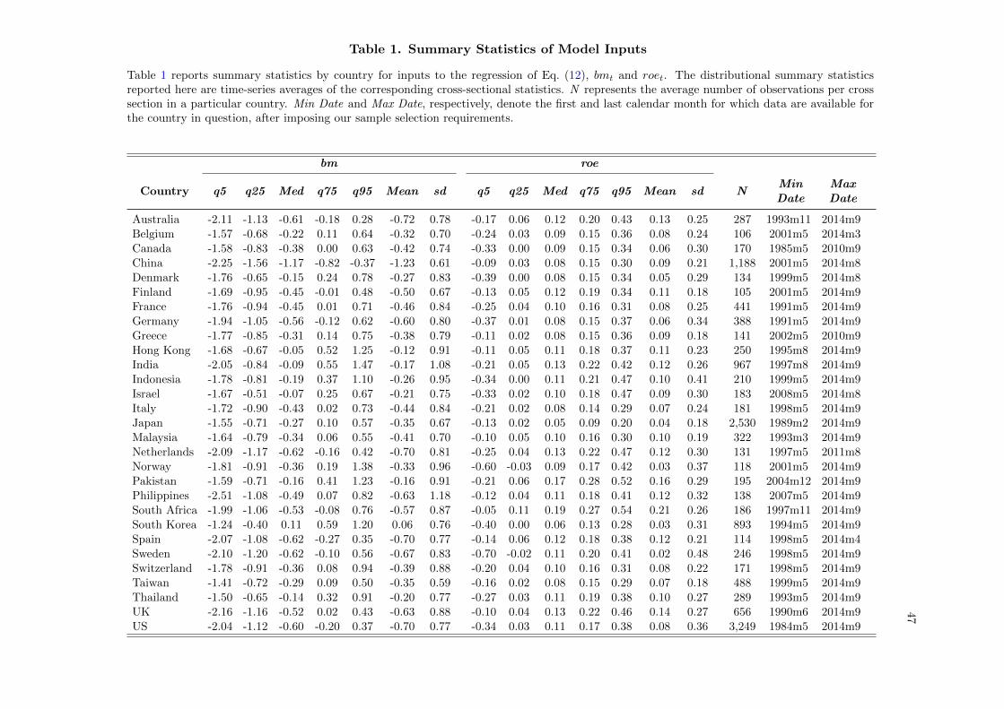
47
Table 1. Summary Statistics of Model Inputs
Table 1 reports summary statistics by country for inputs to the regression of Eq. (12), bmt and roet. The distributional summary statisticsreported here are time-series averages of the corresponding cross-sectional statistics. N represents the average number of observations per crosssection in a particular country. Min Date and Max Date, respectively, denote the first and last calendar month for which data are available forthe country in question, after imposing our sample selection requirements.
bm roe
Country q5 q25 Med q75 q95 Mean sd q5 q25 Med q75 q95 Mean sd NMinDate
MaxDate
Australia -2.11 -1.13 -0.61 -0.18 0.28 -0.72 0.78 -0.17 0.06 0.12 0.20 0.43 0.13 0.25 287 1993m11 2014m9Belgium -1.57 -0.68 -0.22 0.11 0.64 -0.32 0.70 -0.24 0.03 0.09 0.15 0.36 0.08 0.24 106 2001m5 2014m3Canada -1.58 -0.83 -0.38 0.00 0.63 -0.42 0.74 -0.33 0.00 0.09 0.15 0.34 0.06 0.30 170 1985m5 2010m9China -2.25 -1.56 -1.17 -0.82 -0.37 -1.23 0.61 -0.09 0.03 0.08 0.15 0.30 0.09 0.21 1,188 2001m5 2014m8Denmark -1.76 -0.65 -0.15 0.24 0.78 -0.27 0.83 -0.39 0.00 0.08 0.15 0.34 0.05 0.29 134 1999m5 2014m8Finland -1.69 -0.95 -0.45 -0.01 0.48 -0.50 0.67 -0.13 0.05 0.12 0.19 0.34 0.11 0.18 105 2001m5 2014m9France -1.76 -0.94 -0.45 0.01 0.71 -0.46 0.84 -0.25 0.04 0.10 0.16 0.31 0.08 0.25 441 1991m5 2014m9Germany -1.94 -1.05 -0.56 -0.12 0.62 -0.60 0.80 -0.37 0.01 0.08 0.15 0.37 0.06 0.34 388 1991m5 2014m9Greece -1.77 -0.85 -0.31 0.14 0.75 -0.38 0.79 -0.11 0.02 0.08 0.15 0.36 0.09 0.18 141 2002m5 2010m9Hong Kong -1.68 -0.67 -0.05 0.52 1.25 -0.12 0.91 -0.11 0.05 0.11 0.18 0.37 0.11 0.23 250 1995m8 2014m9India -2.05 -0.84 -0.09 0.55 1.47 -0.17 1.08 -0.21 0.05 0.13 0.22 0.42 0.12 0.26 967 1997m8 2014m9Indonesia -1.78 -0.81 -0.19 0.37 1.10 -0.26 0.95 -0.34 0.00 0.11 0.21 0.47 0.10 0.41 210 1999m5 2014m9Israel -1.67 -0.51 -0.07 0.25 0.67 -0.21 0.75 -0.33 0.02 0.10 0.18 0.47 0.09 0.30 183 2008m5 2014m8Italy -1.72 -0.90 -0.43 0.02 0.73 -0.44 0.84 -0.21 0.02 0.08 0.14 0.29 0.07 0.24 181 1998m5 2014m9Japan -1.55 -0.71 -0.27 0.10 0.57 -0.35 0.67 -0.13 0.02 0.05 0.09 0.20 0.04 0.18 2,530 1989m2 2014m9Malaysia -1.64 -0.79 -0.34 0.06 0.55 -0.41 0.70 -0.10 0.05 0.10 0.16 0.30 0.10 0.19 322 1993m3 2014m9Netherlands -2.09 -1.17 -0.62 -0.16 0.42 -0.70 0.81 -0.25 0.04 0.13 0.22 0.47 0.12 0.30 131 1997m5 2011m8Norway -1.81 -0.91 -0.36 0.19 1.38 -0.33 0.96 -0.60 -0.03 0.09 0.17 0.42 0.03 0.37 118 2001m5 2014m9Pakistan -1.59 -0.71 -0.16 0.41 1.23 -0.16 0.91 -0.21 0.06 0.17 0.28 0.52 0.16 0.29 195 2004m12 2014m9Philippines -2.51 -1.08 -0.49 0.07 0.82 -0.63 1.18 -0.12 0.04 0.11 0.18 0.41 0.12 0.32 138 2007m5 2014m9South Africa -1.99 -1.06 -0.53 -0.08 0.76 -0.57 0.87 -0.05 0.11 0.19 0.27 0.54 0.21 0.26 186 1997m11 2014m9South Korea -1.24 -0.40 0.11 0.59 1.20 0.06 0.76 -0.40 0.00 0.06 0.13 0.28 0.03 0.31 893 1994m5 2014m9Spain -2.07 -1.08 -0.62 -0.27 0.35 -0.70 0.77 -0.14 0.06 0.12 0.18 0.38 0.12 0.21 114 1998m5 2014m4Sweden -2.10 -1.20 -0.62 -0.10 0.56 -0.67 0.83 -0.70 -0.02 0.11 0.20 0.41 0.02 0.48 246 1998m5 2014m9Switzerland -1.78 -0.91 -0.36 0.08 0.94 -0.39 0.88 -0.20 0.04 0.10 0.16 0.31 0.08 0.22 171 1998m5 2014m9Taiwan -1.41 -0.72 -0.29 0.09 0.50 -0.35 0.59 -0.16 0.02 0.08 0.15 0.29 0.07 0.18 488 1999m5 2014m9Thailand -1.50 -0.65 -0.14 0.32 0.91 -0.20 0.77 -0.27 0.03 0.11 0.19 0.38 0.10 0.27 289 1993m5 2014m9UK -2.16 -1.16 -0.52 0.02 0.43 -0.63 0.88 -0.10 0.04 0.13 0.22 0.46 0.14 0.27 656 1990m6 2014m9US -2.04 -1.12 -0.60 -0.20 0.37 -0.70 0.77 -0.34 0.03 0.11 0.17 0.38 0.08 0.36 3,249 1984m5 2014m9

48
Table 2. Summary Statistics of Estimated Coefficients
Table 2 reports the coefficients on bmt and roet. The coefficients are estimated by Fama and MacBeth(1973) cross-sectional regressions, in which monthly log-returns are regressed on firm characteristics foreach calendar month. We assume accounting data is known four months after the fiscal-year end date.Publicly available financial data on book values and ROE are matched to one-month-ahead returns fortwelve months, starting four months after the fiscal-year end date as in Lewellen (2015). The estimationuses the cross-section of firms in a given country for a particular calendar month. Columns (1)–(3) reportthe Fama-MacBeth coefficients and standard errors (in square brackets below coefficients). Column (4)reports the average number of firms per cross section, column (5) reports the total number of monthsincluded in the Fama-Macbeth estimates, and column (6) reports the average of the cross-sectional-regression adjusted R2 values. Levels of significance are indicated by *, **, and ***, representing 10percent, 5 percent, and 1 percent, respectively.
(1) (2) (3) (4) (5) (6)
Country bm roe cons NNo. ofPeriods
Adj R2
Australia 0.0033*** 0.0103*** 0.0048* 286 252 0.019[0.001] [0.004] [0.002]
Belgium 0.0047*** 0.0242*** 0.0015 106 139 0.020[0.001] [0.006] [0.004]
Canada -0.0004 0.0095** -0.0004 170 300 0.016[0.001] [0.004] [0.003]
China 0.0051*** 0.0031 0.0086 1,182 161 0.022[0.001] [0.005] [0.008]
Denmark 0.0000 0.0136*** 0.0003 134 185 0.028[0.002] [0.004] [0.004]
Finland 0.0091*** 0.0318*** -0.0014 106 108 0.039[0.002] [0.009] [0.005]
France 0.0030*** 0.0155*** 0.0021 440 282 0.019[0.001] [0.003] [0.003]
Germany 0.0025*** 0.0103*** -0.0016 387 282 0.015[0.001] [0.002] [0.003]
Greece 0.0006 0.0287*** -0.0133 141 100 0.021[0.002] [0.008] [0.009]
HongKong 0.0067*** 0.0223*** -0.0015 250 229 0.020[0.001] [0.007] [0.005]
India 0.0016 0.0129** 0.0026 963 207 0.029[0.002] [0.005] [0.007]
Indonesia 0.0060*** 0.0136*** 0.0090 210 186 0.015[0.002] [0.003] [0.006]
Israel 0.0007 0.0234*** -0.0008 182 77 0.017[0.002] [0.006] [0.009]
Italy 0.0021** 0.0182*** -0.0019 181 198 0.025[0.001] [0.004] [0.004]

49
Table 2. Continued
(1) (2) (3) (4) (5) (6)
Country bm roe cons NNo. ofPeriods
Adj R2
Japan 0.0067*** 0.0069*** -0.0007 2,522 309 0.017[0.001] [0.002] [0.004]
Malaysia 0.0064*** 0.0238*** 0.0009 321 260 0.017[0.001] [0.005] [0.006]
Netherlands 0.0034* 0.0113** 0.0002 131 172 0.030[0.002] [0.006] [0.004]
Norway 0.0013 0.0211*** 0.0014 118 152 0.024[0.001] [0.006] [0.004]
Pakistan -0.0004 0.0105** 0.0120* 195 116 0.022[0.002] [0.005] [0.006]
Philippines 0.0036** 0.0100* 0.0095 138 79 0.010[0.002] [0.006] [0.006]
South Africa 0.0027** 0.0010 0.0098*** 185 204 0.015[0.001] [0.004] [0.003]
South Korea 0.0097*** 0.0159*** -0.0054 889 246 0.022[0.002] [0.004] [0.006]
Spain 0.0029** 0.0256*** 0.0001 115 184 0.031[0.001] [0.007] [0.004]
Sweden 0.0012 0.0120*** 0.0001 246 198 0.029[0.001] [0.003] [0.004]
Switzerland 0.0022** 0.0080* 0.0027 170 198 0.024[0.001] [0.005] [0.003]
Taiwan 0.0063** 0.0314*** -0.0015 486 186 0.048[0.003] [0.007] [0.007]
Thailand 0.0074*** 0.0208*** 0.0002 289 258 0.019[0.001] [0.006] [0.005]
UK 0.0022*** 0.0083*** 0.0045* 654 293 0.011[0.001] [0.002] [0.003]
US 0.0030*** 0.0047*** 0.0065** 3,244 366 0.011[0.001] [0.001] [0.003]

50Table 3. Summary Statistics of Expected Return Proxies
Table 3 columns (1)-(3) and (5)-(9) report summary statistics by country for the monthly ERPs calculated using Eq. (12). The table reports
time-series averages of the corresponding cross-sectional statistics. Expected-return proxies for a particular calendar month are calculated using
firm characteristics and the cumulative rolling average of the estimated cross-sectional coefficients as of the end of the previous calendar month.
For calculating cumulative averages, we use a burn-in period of forty months. Column(4) reports the time-series average of the cross-sectional
mean of a proxy for expected simple returns, computed as Et[Ri,t+1] = exp(µi,t+0.5× σ2i,t+1), where µi,t is our expected log return estimate, and
σ2i,t+1 is an estimate of the expected volatility in log returns based on the average squared daily returns from the prior month scaled by 252/12.
Finally, the last three columns report the time-series averages of the cross-sectional mean realized log monthly returns, variance of realized log
monthly returns, and mean realized simple monthly returns.
(1) (2) (3) (4) (5) (6) (7) (8) (9) (10) (11) (12)q5 q25 Mean Mean Median q75 q95 sd N Mean Variance Mean
(Simple) Log Returns Log Returns Simple Returns
Australia -0.0034 0.0029 0.0050 0.0106 0.0069 0.0095 0.0043 0.0053 268 0.0040 0.0116 0.0095Belgium -0.0061 0.0013 0.0037 0.0086 0.0055 0.0098 0.0030 0.0057 76 0.0021 0.0119 0.0071Canada -0.0043 0.0007 0.0020 0.0156 0.0032 0.0062 0.0016 0.0047 153 -0.0002 0.0280 0.0115China -0.0105 -0.0054 -0.0027 0.0074 -0.0004 0.0028 -0.0032 0.0048 1,118 0.0028 0.0184 0.0123Denmark -0.0023 0.0027 0.0040 0.0129 0.0049 0.0069 0.0035 0.0033 110 -0.0003 0.0183 0.0074Finland -0.0120 -0.0043 0.0006 0.0066 0.0051 0.0117 0.0003 0.0078 68 0.0024 0.0141 0.0078France -0.0031 0.0023 0.0036 0.0110 0.0047 0.0074 0.0030 0.0047 421 0.0018 0.0144 0.0084Germany -0.0072 -0.0033 -0.0020 0.0072 -0.0008 0.0017 -0.0023 0.0035 366 -0.0029 0.0170 0.0041Greece -0.0126 -0.0064 -0.0042 0.0058 -0.0019 0.0055 -0.0041 0.0072 93 -0.0104 0.0170 -0.0012HongKong -0.0167 -0.0079 -0.0047 0.0043 -0.0017 0.0038 -0.0055 0.0088 229 0.0010 0.0199 0.0125India -0.0043 0.0002 0.0014 0.0148 0.0026 0.0053 0.0011 0.0041 928 0.0048 0.0292 0.0207Indonesia -0.0038 0.0026 0.0064 0.0277 0.0102 0.0149 0.0061 0.0070 182 0.0082 0.0466 0.0263Israel -0.0108 -0.0043 -0.0028 0.0003 -0.0016 0.0036 -0.0031 0.0063 108 0.0013 0.0132 0.0105Italy -0.0077 -0.0034 -0.0019 0.0028 -0.0006 0.0017 -0.0023 0.0041 150 -0.0025 0.0107 0.0033Japan -0.0110 -0.0051 -0.0020 0.0064 0.0006 0.0040 -0.0026 0.0049 2,371 -0.0035 0.0176 0.0041Malaysia -0.0075 -0.0018 0.0010 0.0073 0.0033 0.0064 0.0004 0.0050 301 0.0008 0.0310 0.0122Netherlands -0.0081 -0.0026 0.0000 0.0101 0.0021 0.0048 -0.0007 0.0051 98 -0.0014 0.0190 0.0101Norway -0.0080 0.0027 0.0051 0.0074 0.0071 0.0111 0.0040 0.0068 88 0.0014 0.0152 0.0056Pakistan 0.0047 0.0076 0.0092 0.0148 0.0106 0.0132 0.0091 0.0030 148 0.0137 0.0253 0.0102Philippines -0.0013 0.0071 0.0090 0.0199 0.0107 0.0132 0.0081 0.0057 78 0.0044 0.0197 0.0237South Africa -0.0023 0.0034 0.0063 0.0196 0.0086 0.0132 0.0060 0.0050 158 0.0092 0.0251 0.0150South Korea -0.0227 -0.0135 -0.0087 0.0129 -0.0045 0.0007 -0.0096 0.0078 855 -0.0041 0.0159 0.0162Spain -0.0071 0.0004 0.0025 0.0067 0.0042 0.0075 0.0018 0.0066 90 0.0008 0.0099 0.0059Sweden -0.0132 -0.0029 -0.0007 0.0091 0.0010 0.0039 -0.0019 0.0067 212 -0.0012 0.0222 0.0079Switzerland -0.0028 -0.0003 0.0012 0.0068 0.0023 0.0046 0.0010 0.0027 145 0.0020 0.0117 0.0067Taiwan -0.0147 -0.0072 -0.0049 0.0006 -0.0032 -0.0001 -0.0059 0.0064 449 -0.0002 0.0150 0.0088Thailand -0.0263 -0.0106 -0.0058 0.0114 -0.0023 0.0030 -0.0076 0.0111 272 0.0021 0.0331 0.0150UK 0.0023 0.0043 0.0053 0.0095 0.0063 0.0082 0.0053 0.0026 599 0.0042 0.0083 0.0096US 0.0014 0.0045 0.0059 0.0173 0.0069 0.0084 0.0055 0.0027 3,004 0.0051 0.0219 0.0145
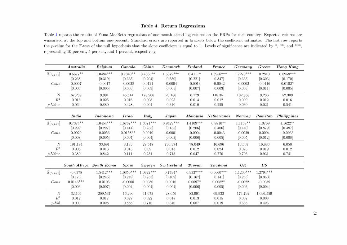
51
Table 4. Return Regressions
Table 4 reports the results of Fama-MacBeth regressions of one-month-ahead log returns on the ERPs for each country. Expected returns are
winsorized at the top and bottom one-percent. Standard errors are reported in brackets below the coefficient estimates. The last row reports
the p-value for the F-test of the null hypothesis that the slope coefficient is equal to 1. Levels of significance are indicated by *, **, and ***,
representing 10 percent, 5 percent, and 1 percent, respectively.
Australia Belgium Canada China Denmark Finland France Germany Greece Hong Kong
E[ri,t+1] 0.5577** 1.0484*** 0.7340** 0.4085** 1.5072*** 0.4111* 1.3956*** 1.7270*** 0.2810 0.8958***[0.238] [0.319] [0.335] [0.204] [0.530] [0.221] [0.347] [0.333] [0.303] [0.170]
Cons 0.0007 -0.0017 -0.0028 0.0121 -0.0004 -0.0013 -0.0042 -0.0002 -0.0116 0.0102*[0.003] [0.005] [0.003] [0.009] [0.005] [0.007] [0.003] [0.003] [0.011] [0.005]
N 67,239 9,991 45,514 178,906 20,186 6,779 118,351 102,838 9,236 52,309R2 0.016 0.025 0.016 0.008 0.025 0.014 0.012 0.009 0.012 0.016
p-Value 0.064 0.880 0.428 0.004 0.340 0.010 0.255 0.030 0.021 0.541
India Indonesia Israel Italy Japan Malaysia Netherlands Norway Pakistan Philippines
E[ri,t+1] 0.7374** 1.0454*** 1.6767*** 1.3071*** 0.9429*** 1.4109*** 0.8810** 1.1139** 1.0769 1.1622**[0.299] [0.227] [0.414] [0.255] [0.155] [0.206] [0.406] [0.440] [0.879] [0.487]
Cons 0.0029 0.0056 0.0158** 0.0010 -0.0001 -0.0004 -0.0043 -0.0029 0.0004 -0.0033[0.008] [0.005] [0.007] [0.004] [0.003] [0.006] [0.005] [0.005] [0.012] [0.008]
N 191,194 33,691 8,183 29,548 730,374 78,049 16,696 13,307 16,883 6,050R2 0.008 0.013 0.015 0.02 0.013 0.012 0.024 0.025 0.019 0.012
p-Value 0.380 0.842 0.111 0.231 0.713 0.047 0.770 0.796 0.931 0.741
South Africa South Korea Spain Sweden Switzerland Taiwan Thailand UK US
E[ri,t+1] -0.0378 1.5412*** 1.0350*** 1.0922*** 0.7494* 0.9327*** 0.6660*** 1.1200*** 1.2794***[0.170] [0.245] [0.249] [0.253] [0.409] [0.167] [0.141] [0.255] [0.350]
Cons 0.0146*** 0.0105 -0.0000 0.0030 0.0016 0.0097* 0.0082* -0.0022 -0.0039[0.003] [0.007] [0.004] [0.004] [0.004] [0.006] [0.005] [0.003] [0.004]
N 32,104 209,537 16,290 41,673 28,656 82,991 69,932 174,792 1,096,559R2 0.012 0.017 0.027 0.022 0.018 0.013 0.015 0.007 0.008
p-Val 0.000 0.028 0.888 0.716 0.540 0.687 0.019 0.638 0.425
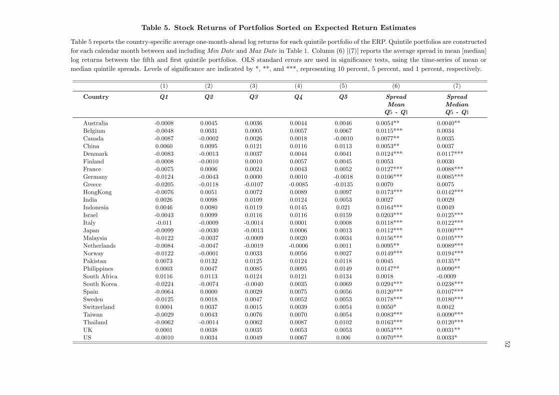
52
Table 5. Stock Returns of Portfolios Sorted on Expected Return Estimates
Table 5 reports the country-specific average one-month-ahead log returns for each quintile portfolio of the ERP. Quintile portfolios are constructed
for each calendar month between and including Min Date and Max Date in Table 1. Column (6) [(7)] reports the average spread in mean [median]
log returns between the fifth and first quintile portfolios. OLS standard errors are used in significance tests, using the time-series of mean or
median quintile spreads. Levels of significance are indicated by *, **, and ***, representing 10 percent, 5 percent, and 1 percent, respectively.
(1) (2) (3) (4) (5) (6) (7)
Country Q1 Q2 Q3 Q4 Q5 Spread SpreadMean Median
Q5 - Q1 Q5 - Q1
Australia -0.0008 0.0045 0.0036 0.0044 0.0046 0.0054** 0.0040**Belgium -0.0048 0.0031 0.0005 0.0057 0.0067 0.0115*** 0.0034Canada -0.0087 -0.0002 0.0026 0.0018 -0.0010 0.0077** 0.0035China 0.0060 0.0095 0.0121 0.0116 0.0113 0.0053** 0.0037Denmark -0.0083 -0.0013 0.0037 0.0044 0.0041 0.0124*** 0.0117***Finland -0.0008 -0.0010 0.0010 0.0057 0.0045 0.0053 0.0030France -0.0075 0.0006 0.0024 0.0043 0.0052 0.0127*** 0.0088***Germany -0.0124 -0.0043 0.0000 0.0010 -0.0018 0.0106*** 0.0085***Greece -0.0205 -0.0118 -0.0107 -0.0085 -0.0135 0.0070 0.0075HongKong -0.0076 0.0051 0.0072 0.0089 0.0097 0.0173*** 0.0142***India 0.0026 0.0098 0.0109 0.0124 0.0053 0.0027 0.0029Indonesia 0.0046 0.0080 0.0119 0.0145 0.021 0.0164*** 0.0049Israel -0.0043 0.0099 0.0116 0.0116 0.0159 0.0203*** 0.0125***Italy -0.011 -0.0009 -0.0014 0.0001 0.0008 0.0118*** 0.0122***Japan -0.0099 -0.0030 -0.0013 0.0006 0.0013 0.0112*** 0.0100***Malaysia -0.0122 -0.0037 -0.0009 0.0020 0.0034 0.0156*** 0.0105***Netherlands -0.0084 -0.0047 -0.0019 -0.0006 0.0011 0.0095** 0.0089***Norway -0.0122 -0.0001 0.0033 0.0056 0.0027 0.0149*** 0.0194***Pakistan 0.0073 0.0132 0.0125 0.0124 0.0118 0.0045 0.0135**Philippines 0.0003 0.0047 0.0085 0.0095 0.0149 0.0147** 0.0090**South Africa 0.0116 0.0113 0.0124 0.0121 0.0134 0.0018 -0.0009South Korea -0.0224 -0.0074 -0.0040 0.0035 0.0069 0.0294*** 0.0238***Spain -0.0064 0.0000 0.0029 0.0075 0.0056 0.0120*** 0.0107***Sweden -0.0125 0.0018 0.0047 0.0052 0.0053 0.0178*** 0.0180***Switzerland 0.0004 0.0037 0.0015 0.0039 0.0054 0.0050* 0.0042Taiwan -0.0029 0.0043 0.0076 0.0070 0.0054 0.0083*** 0.0090***Thailand -0.0062 -0.0014 0.0062 0.0087 0.0102 0.0163*** 0.0120***UK 0.0001 0.0038 0.0035 0.0053 0.0053 0.0053*** 0.0031**US -0.0010 0.0034 0.0049 0.0067 0.006 0.0070*** 0.0033*

53
Table 6. Return Regressions: Factor-Based-Model Expected-Return Estimates
Table 6 reports the results of Fama-MacBeth regressions of future simple returns on different ERPs. Columns under FF Global and FF Regional
report regression of realized simple returns on ERPs generated using firm-specific loadings on the Fama-French global four factors and the
regional four factors, respectively. Expected factor returns are estimated based on trailing 40-month averages, and factor loadings are estimated
based using data available in the 40 months prior to the forecast date. For comparison, we create proxies of expected simple returns computed
as Et[Ri,t+1] = exp(µi,t + 0.5 × σ2i,t+1), where µi,t is our expected log return estimate, and σ2
i,t+1 is an estimate of the volatility in log returns
based on the average squared daily returns from the prior month scaled by 252/12. Regression-based tests using simple returns and these proxies
are reported in columns under the heading CLW. The analyses are conducted on a common set of firm-year observations for which all ERPs are
available. All ERPs are winsorized at the top and bottom one percent. Columns under the heading E[ri,t+1] reports the slope coefficient on the
ERP, Cons reports the coefficient on the constant term, and p reports p-values corresponding to the F-test of the null that the slope coefficient
is equal to 1. Levels of significance are indicated by *, **, and ***, representing 10 percent, 5 percent, and 1 percent, respectively.
CLW FF Global FF Regional
Country E[ri,t+1] Cons p E[ri,t+1] Cons p E[ri,t+1] Cons p N
Australia 0.5530** 0.0082** 0.047 -0.0772 0.0026 0.000 -0.0082 0.0118*** 0.000 64,374Belgium 0.6807** 0.0045 0.227 -0.2375 -0.0185* 0.000 0.0284 0.0070 0.004 9,654Canada 0.4700*** 0.0059** 0.000 0.0019 0.0234 0.000 -0.2233*** 0.0123*** 0.000 43,212China 3.5899*** -0.0073 0.000 -0.0100 0.0271** 0.000 -0.1794 0.0222** 0.000 172,531Denmark 1.0543*** -0.0006 0.816 -0.3165** 0.0370*** 0.000 -0.0174 0.0124** 0.000 19,089Finland 0.4946** 0.0028 0.039 -0.1025 0.0167 0.000 -1.1804** 0.0005 0.000 6,438France 1.0689*** -0.0008 0.715 0.0194 0.0101 0.000 -0.0187 0.0083** 0.000 112,612Germany 0.7193*** 0.0016 0.121 -0.0255 -0.0126 0.000 -0.1012 0.0048 0.000 99,671Greece 1.0357** -0.0059 0.933 -0.0277 -0.0120 0.000 0.7443 0.0021 0.638 9,058HongKong 2.2628*** 0.0070* 0.000 -0.2135* -0.0029 0.000 0.1131 0.0140*** 0.000 50,424India 3.7759*** -0.0331*** 0.000 -0.0797 0.0232* 0.000 -0.0447 0.0222*** 0.000 183,428Indonesia 2.1836*** -0.0173 0.051 -0.2492** 0.0365*** 0.000 -0.1593 0.0302*** 0.000 30,706Israel 1.3927*** 0.0145 0.372 -0.3088** 0.0188** 0.000 -0.1569 0.0157* 0.000 7,801Italy 2.9696*** 0.0033 0.000 -0.1301 0.0091 0.000 -0.2258 0.0052 0.000 28,681Japan 2.3393*** -0.0069** 0.000 -0.0058 -0.0141 0.000 0.0278 0.0039 0.000 683,671Malaysia 1.7983*** -0.0100* 0.000 -0.0444 0.0055 0.000 0.1053 0.0067 0.000 75,221Netherlands 0.7825*** 0.0071 0.424 -0.2979 0.0120 0.000 0.3090 0.0102* 0.001 16,211Norway 1.3719*** -0.0065 0.109 -0.1321 0.0016 0.000 -0.2061 0.0079 0.000 12,457Pakistan 2.0903*** -0.0221*** 0.005 0.2596* 0.0143* 0.000 -0.0936 0.0163* 0.000 16,179Philippines 1.9876*** -0.0217** 0.023 -0.1057 0.0183** 0.000 0.2794 0.0167* 0.027 5,813South Africa 0.6764*** 0.0103* 0.019 0.0044 0.0403*** 0.000 0.2063 0.0170*** 0.000 30,745South Korea 3.0504*** 0.0011 0.000 -0.0023 0.0278 0.000 -0.0699 0.0160* 0.000 204,707Spain 1.9934*** 0.0002 0.003 -0.1359 -0.0059 0.000 0.3016 0.0095* 0.007 15,847Sweden 1.2380*** 0.0070 0.188 0.0204 0.0142 0.000 -0.0884 0.0143** 0.000 40,511Switzerland 1.0388*** 0.0080** 0.873 -0.1153 -0.0107 0.000 -0.0330 0.0084** 0.000 27,691Taiwan 3.5363*** 0.0147** 0.000 -0.0783 0.0027 0.000 0.1934 0.0157** 0.000 81,252Thailand 1.6473*** 0.0096 0.000 -0.0212 -0.0196 0.000 -0.2078* 0.0172** 0.000 65,056UK 1.0344*** 0.0025 0.873 -0.0126 0.0091 0.000 -0.1291 0.0080*** 0.000 161,469US 0.7782*** 0.0033* 0.051 -0.0924 0.0233* 0.000 -0.0660* 0.0132*** 0.000 1,069,3165-Factor -0.0385 0.0127*** 0.000 1,069,3163-Factor -0.1031* 0.0134*** 0.000 1,069,316

54Table 7. Dividend Payout and Relations between Expected Returns and Accounting-Based Characteristics
Table 7 reports the country-level results on the estimation of (17). We run Fama-MacBeth regressions of future realized annual log stock returns,
rt+1, on firm characteristics, bmt, roet+1, labeled as froe in the table, and payoutt+1, a continuous variable computed as Dividendst+1/Bookt+1.
The variables bm×payout and froe×payoutrepresent interactions of payout with bm and froe, respectively. payout is winsorized at the 1-percent
level. Standard errors are reported in brackets below the coefficient estimates. Levels of significance are indicated by *, **, and ***, representing
10 percent, 5 percent, and 1 percent, respectively.
Australia Belgium Canada China Denmark Finland France Germany Greece Hong Kong
bm 0.0424** 0.0206 0.0602** 0.0721*** 0.0344 0.0947* 0.0554*** 0.0581*** 0.0761** 0.0859***[0.020] [0.042] [0.023] [0.016] [0.033] [0.030] [0.014] [0.021] [0.023] [0.022]
froe 0.1183** 0.4580*** 0.3951*** 0.2718*** 0.4020*** 0.5090*** 0.4231*** 0.2707*** 0.4907*** 0.4655***[0.056] [0.058] [0.101] [0.069] [0.091] [0.072] [0.049] [0.037] [0.091] [0.156]
payout 0.3582 2.1520** -0.1976 -0.6139 1.4684** 1.2045* 0.5462 0.8191*** 2.0232*** 0.8740**[0.214] [0.442] [0.395] [1.162] [0.569] [0.408] [0.320] [0.209] [0.499] [0.343]
bm× payout 0.4629*** 1.4412* 0.2061 0.8498** 1.2337*** 0.6640** -0.0775 0.5326** 1.3149*** 0.4819**[0.151] [0.580] [0.343] [0.361] [0.354] [0.168] [0.291] [0.217] [0.361] [0.214]
froe× payout 1.8429** 1.5300 2.0541 4.8886 3.5593* 1.5894 -0.9048 3.8656** 1.9315 1.1293[0.747] [3.268] [1.547] [3.904] [1.954] [1.816] [1.294] [1.611] [1.241] [1.514]
Cons 0.0927*** -0.1203 0.0312 0.0929 0.0010 -0.1041 0.0224 -0.0038 -0.0820 0.0395[0.031] [0.122] [0.033] [0.091] [0.075] [0.158] [0.043] [0.042] [0.108] [0.044]
N 4,849 424 3,867 14,207 1,886 416 9,707 8,608 1,088 3,965Adj R2 0.086 0.175 0.121 0.091 0.185 0.145 0.128 0.143 0.135 0.130
India Indonesia Israel Italy Japan Malaysia Netherlands Norway Pakistan Philippines
bm 0.0437** 0.1212*** 0.0249 0.0309 0.0594*** 0.0933*** 0.0644* 0.0199 0.0352 0.0480[0.018] [0.019] [0.026] [0.020] [0.010] [0.023] [0.033] [0.021] [0.024] [0.032]
froe 0.0428 0.4699*** 0.3244*** 0.3959*** 0.0677*** 0.3676*** 0.4499*** 0.2972*** 0.2220** 0.1309[0.058] [0.099] [0.055] [0.064] [0.023] [0.119] [0.126] [0.061] [0.075] [0.089]
payout 2.5548*** 1.5426 0.8666** 1.3632*** 1.3688 1.7060** 1.0725*** 1.3328** 0.1186 -0.2669[0.708] [4.648] [0.222] [0.437] [0.807] [0.624] [0.350] [0.509] [0.512] [0.334]
bm× payout 0.6496** 7.3759 1.0607** 1.3288*** 0.9676*** 1.3732*** 0.8743** 1.1769** 0.7299*** 1.3879**[0.230] [11.419] [0.309] [0.393] [0.338] [0.357] [0.301] [0.395] [0.182] [0.378]
froe× payout -0.4167 11.6932 2.4046 3.2815 4.7387** 4.5108** 2.0722 2.0203* 4.3875*** 10.6006***[1.403] [17.377] [1.404] [2.970] [2.027] [1.732] [1.326] [0.960] [1.169] [1.063]
Cons 0.0312 0.0988 0.0167 0.0116 -0.0175 0.0257 -0.0072 0.0122 0.0437 0.1713**[0.085] [0.083] [0.076] [0.067] [0.055] [0.070] [0.062] [0.086] [0.121] [0.030]
N 13,663 2,973 1,060 2,786 60,045 5,917 1,878 1,193 1,658 570Adj R2 0.079 0.146 0.137 0.164 0.058 0.122 0.178 0.131 0.123 0.093

55Table 7. Continued.
South Africa South Korea Spain Sweden Switzerland Taiwan Thailand UK US
bm 0.0649*** 0.0954*** 0.0696** 0.0328 0.0252 0.1377*** 0.1484*** 0.0420*** 0.0571***[0.016] [0.026] [0.024] [0.029] [0.019] [0.034] [0.022] [0.011] [0.014]
froe 0.1977** 0.2752*** 0.5459*** 0.2897*** 0.2940*** 0.7741*** 0.8335*** 0.2037*** 0.1544***[0.077] [0.066] [0.142] [0.054] [0.094] [0.132] [0.176] [0.057] [0.025]
payout 0.0978 1.6930* 0.4924 1.1439*** 0.5812 14.0831 -0.2767 0.3312** 0.0705[0.371] [0.856] [0.393] [0.321] [0.527] [13.795] [0.329] [0.152] [0.138]
bm× payout 0.3029* 3.5678*** 0.7707* 0.7656*** 1.2231*** 31.1406 0.8280*** 0.1066 0.0732[0.162] [0.342] [0.359] [0.178] [0.206] [38.190] [0.268] [0.083] [0.083]
froe× payout 0.9042 14.6233*** 2.6362* 1.8357** 6.6188** 156.3112 5.3548** 0.0851 0.6971***[1.231] [2.748] [1.458] [0.742] [2.416] [141.621] [2.064] [0.208] [0.245]
Cons 0.1144** -0.0758 0.0179 0.0018 0.0038 -0.0085 -0.0274 0.0714** 0.0948***[0.052] [0.103] [0.070] [0.058] [0.060] [0.062] [0.075] [0.028] [0.028]
N 2,922 17,042 1,530 3,828 2,605 7,447 5,784 14,609 92,534Adj R2 0.104 0.154 0.186 0.153 0.161 0.163 0.149 0.069 0.053

56
Table 8. Earnings Quality and Importance of ROE
Table 8 reports the results of OLS and instrumental-variables (IV) regressions of country-level median roe coefficients, from monthly regressions
of Eq. (12), on measures of earnings quality. Our overall earnings quality measure follows Leuz et al. (2003): a simple average of a country’s
in-sample ranks on four dimensions of earnings quality: earnings smoothness, correlation of accruals and cash flows, accruals magnitude, and loss
avoidance. These four variables are defined in Table 9. A higher score on each of these dimensions, and on the overall earnings-quality measure,
implies lower or poorer earnings quality. The leftmost column reports the results of an OLS regression of the median roe coefficients on overall
earnings quality. The second and third columns report the first and second stage results, respectively, of instrumental variables regressions where
earnings quality is instrumented with a measure for a country’s quality of governance institutions. This quality of governance measures combines
information on a country’s Rule of Law, Accountability, Political Stability, Government Effectiveness, and Control of Corruption, as reported by
the World Bank’s Worldwide Governance Indicators project. Rule of Law captures perceptions of the quality of contract enforcement, property
rights, and the courts; Accountability captures perceptions of the extent to which citizens have the ability to exert their voices and influence
to create accountability in society, including freedom to select their government and the presence of a free media; Political Stability measures
perceptions of the likelihood of political instability; Government Effectiveness captures perceptions of the quality of public services and the
robustness of the policy formulation process; and Control of Corruption captures perceptions of the extent to which public power is exercised
for private benefits. We take the median value of each variable over the relevant time frame for each country and then standardize each measure
using the cross-section of countries. Our final country-level measure is the simple average of these standardized measures. In the last column we
report reduced-form versions of the IV estimation. The F-statistic on the instrument is reported in the last row. In each of these regressions we
control for the log of a given country’s median total market capitalization over the relevant time frame. Levels of significance are indicated by
*, **, and ***, representing 10 percent, 5 percent, and 1 percent, respectively.
OLS IV IV ReducedFirst Stage Second Stage Form
Poor Information Quality (Leuz et al., 2003) -0.0001 -0.0007**[0.000] [0.000]
Quality of Governance Institutions -3.9260*** 0.0027*[1.264] [0.001]
Log Market Size -0.0023*** -0.1859 -0.0030*** -0.0029***[0.001] [0.883] [0.001] [0.001]
Constant 0.0750*** 20.6885 0.1041*** 0.0898***[0.023] [23.082] [0.025] [0.018]
Observations 25 25 25 25First Stage F 9.65

57Table 9. Earnings Quality and Importance of ROE: Alternative Measures
Table 9 reports the same specifications reported in Table 8 but uses Leuz et al. (2003)’s four measures of poor Information quality. Variability
measures the extent to which a country’s firms engage in earnings smoothing. In descending order, we rank each country’s median ratio of
firm-level standard deviation of operating earnings to the firm-level standard deviation of cash-flow from operations. A lower ratio implies a
greater degree of earnings smoothing and thus lower earnings quality, resulting in a higher rank in Poor Information Quality. Correlation also
measures the extent of earnings smoothing in a country. Across countries, in ascending order, we rank the magnitude of the contemporaneous
correlation between changes in accounting accruals and changes in operating cash flows. This correlation is estimated by pooling all firm-years
within a country. A greater magnitude of correlation implies greater earnings smoothing and lower earnings quality, resulting in a higher rank
on Poor Information Quality. Accruals Magnitude proxies for the extent of the use of accruals to manage earnings. We rank, in ascending order,
the median of the absolute value of firm accruals scaled by the absolute value of firm cash-flow from operations. A higher median ratio implies
a greater use of accruals in managing earnings and lower earnings quality, resulting in a higher rank on Poor Information Quality. Lastly the
Small Loss Avoidance measure ranks across countries, in ascending order, the ratio of instances of small profits to instances of small losses:
this ratio is calculated by pooling all firm-years within a country. Small profits and small losses are calculated using earnings scaled by total
assets. Small losses are defined as in the range [−0.01, 0) and small profits are defined as in the range [0.00, 0.01]. A higher ratio implies greater
use of managerial discretion in managing earnings and lower earnings quality, and results in a higher rank in Poor Information Quality. Our
instruments and control variables remain the same as in Table 8. Levels of significance are indicated by +, *, **, and ***, representing 15
percent, 10 percent, 5 percent, and 1 percent, respectively.
Variability Correlation Accruals Magnitude Small Loss AvoidanceOLS IV IV OLS IV IV OLS IV IV OLS IV IV
First Stage Second Stage First Stage Second Stage First Stage Second Stage First Stage Second Stage
Poor Information Quality 0.0001 -0.0009 0.0000 -0.0006* -0.0002 -0.0006** -0.0000 -0.0008*[0.000] [0.001] [0.000] [0.000] [0.000] [0.000] [0.000] [0.000]
Quality of Governance -2.9232 -4.5851*** -4.8061*** -3.3898+[2.059] [1.537] [1.474] [2.145]
Log Market Size -0.0022*** -0.2771 -0.0032** -0.0022*** 0.0738 -0.0029*** -0.0027*** -1.4518+ -0.0037*** -0.0022*** 0.9117 -0.0022**[0.001] [1.332] [0.001] [0.001] [1.253] [0.001] [0.001] [0.919] [0.001] [0.001] [1.142] [0.001]
Constant 0.0701*** 22.4796 0.1107*** 0.0725*** 14.2393 0.0982*** 0.0860*** 53.8144** 0.1203*** 0.0731*** -7.7792 0.0835***[0.021] [35.373] [0.041] [0.019] [33.039] [0.030] [0.027] [24.410] [0.025] [0.018] [30.393] [0.023]
Observations 25 25 25 25 25 25 25 25 25 25 25 25First Stage F 2.02 8.90 10.63 2.50