Accelerator Based Magnetic Monopole Search Experiments (Overview)

Vasily Dzhordzhadze, Praveen Chaudhari∗, Peter Cameron, Nicholas D’Imperio, Veljko Radeka, Pavel Rehak, Margareta Rehak, Sergio Rescia, Yannis Semertzidis, John Sondericker, and Peter Thieberger.

Brookhaven National Laboratory

ABSTRACT We present an overview of accelerator-based searches for magnetic monopoles and we show

why such searches are important for modern particle physics. Possible properties of monopoles are reviewed as well as experimental methods used in the search for them at accelerators. Two types of experimental methods, direct and indirect are discussed. Finally, we describe proposed magnetic monopole search experiments at RHIC and LHC.

Content

1. Magnetic Monopole characteristics 2. Experimental techniques 3. Monopole Search experiments 4. Magnetic Monopoles in virtual processes 5. Future experiments 6. Summary

1. Magnetic Monopole characteristics The magnetic monopole puzzle remains one of the fundamental and unsolved problems in physics. This problem has a along history. The military engineer Pierre de Maricourt [1] in1269 was breaking magnets, trying to separate their poles. P. Curie assumed the existence of single magnetic poles [2]. A real breakthrough happened after P. Dirac’s approach to the solution of the electron charge quantization problem [3]. Before Dirac, J. Maxwell postulated his fundamental laws of electrodynamics [4], which represent a complete description of all known classical electromagnetic phenomena. Together with the Lorenz force law and the Newton equations of motion, they describe all the classical dynamics of interacting charged particles and electromagnetic fields. In analogy to electrostatics one can add a magnetic charge, by introducing a magnetic charge density, thus magnetic fields are no longer due solely to the motion of an electric charge and in Maxwell equation a magnetic current will appear in analogy to the electric current. The complete set of symmetrized Maxwell equations will have the form:

∗ Spokesperson

1

where indices m and e label electric and magnetic quantities. These modification of the Maxwell equations do not necessarily imply physics beyond the standard electrodynamics, because symmetrized Maxwell equations are invariant under a duality transformation (ξ∈R):

he origin agnetic

which switches electric and magnetic quantities. The extended Maxwell equations can be used

ith electric

The symmetries of ρm under both spatial inversion and time reversal are opposite of those of ρe.

In 1909, Robert Milliken discovered the quantization of electric charge by carrying out his

f

T al Maxwell equations are recovered if all particles have the same ratio of mcharge to electric charge, which can be set to zero by the appropriate choice of the angle ξ. A special case which is useful for the duality transformations is when ξ=π/2. The extended Maxwell equations are invariant under the transformation:

to derive monopole versions of formulas, which are familiar from standard classical electrodynamics. The symmetry suggests a generalized Lorentz force for a particle wcharge e and magnetic charge g:

As a consequence, if dyons, particles with both electric and magnetic charge exists, then space inversion and time reversal are no longer valid symmetries. Symmetry always played a key role in physics and it is therefore a motivation for “inventing” the magnetic charge. famous oil drop experiment. Today the experimental accuracy of the electric charge quantization is [5]: | Qe++Qe-|/e<4x10-8, |Qp++Qp-|/ /e<1x10-8 and |Qp+Qe|/e<1x10-21. This fact o

2

electric charge quantization remains mysterious even today. Its explanation is one of the natures best kept secrets. In 1931, P. Dirac proposed that particles carrying a magnetic charge, or magnetic monopoles should exist. Dirac showed that the phase unobservability in quantum mechanics, permitted singularities, which manifest themselves as a sources of magnetic fieldjust as point electric monopoles were sources of electric fields. This was only possible if the

s,

.5e, |n|=1, 2, 3, … r n=2 according to

n

pole.

tric

y

The coupling constant, related to the magnetic monopole interaction is

heoretical consideration of

he possible existence of magnetic monopoles received a strong boost in 1974 in works of

t was

s and

s

t the same time some authors showed [9, 10], that the unification scale can be significantly

product of electric and magnetic charges is quantized. Dirac established the basic relation between the elementary electric charge e and basic magnetic charge g: eg = nħc/2, where n=+/-1, +/-2, +/-3, … From this equation it follows that the magnetic charge g = nħc/2e = ne/2α = (137/2) ne = 68.5en = gDn, gD= 68The minimum value of the quantization number is n =1 according to Dirac oSchwinger [6]. However, if quarks charge are considered as elementary electric charge, then this magnitude become n=3, 6 respectively. Within this approach, for n=1 and the basic electrocharge of the electron, the theoretical minimum magnetic charge is gD= 68.5e, which is known as a Dirac magnetic charge. It is assumed that magnetic charge, like electric charge, is absolutelyconserved, so the lightest magnetically charged particle is stable, unless annihilated by its antiparticle and magnetic monopoles are always produced in pairs, monopole and antimonoThe quantization of electric charge in nature is well established fact, but it remains still mysterious. The discovery of just a single monopole will explain the quantization of eleccharge. At the same time, as we mentioned above, the existence of magnetic charge and magnetic current will make Maxwell’s equations symmetric, which is not forbidden by an known principles of physics. We should admit, that this symmetry is not exact, because of differences of electric and magnetic charges.

g2/ħc = e2/ħc [g/e]2 = 1/137 [137/2]2 = 34.25 .

For a minimal magnetic charge, this value is >>1. This means that tmagnetic monopoles has serious difficulties. We will discuss this problem in more detail in chapter 5.

T t’Hooft and Polyakov [7,8] related to the Grand Unification Theories (GUT). They independently discovered monopole solutions in the SO(3) Georgi-Glashow model. I

demonstrated that any scheme of Grand Unification with an electromagnetic U(1) subgroup embedded into a semi-simple gauge-group, which becomes spontaneously broken by the Higgs mechanism, possessed a monopole solution. The monopole’s mass mW of standard GUT is related to the mass of the carriers X, Y of the unified interactions: mM ≥ mX/G, where G is the dimensionless coupling constant at energies E ≈ mX . In GUTs with mX ≈ 1014 - 1015 GeV and G ≈ 0.025, mM ≥ 1016 - 1017 GeV. This is a very big mascan never be produced at any man-made accelerators existing or future. They could only have been produced in the firsts moments of the Universe creation and should be searched for in the penetrating cosmic radiation. The most recent search for GUT monopoles in the cosmic radiation was performed by the MACRO detector, which uses three type of detector(liquid scintillators, limited streamer tubes and nuclear track detectors). Alowered (even to the TeV scale) through the appearance of the extra dimensions. This means that magnetic monopoles can be searched for at modern future accelerators like LCH and

3

ILC. For the mass prediction of the magnetic monopoles there exists other estimation, based

eoretical

able 1. Magnetic monopole mass prediction in different theoretical models.

heory Mass GeV Reference

on equality of classical radiuses of electron and magnetic monopoles re=e2/mec2 = rM=g2/mMc2

and mM = 2.4 Gev/c2. In addition to the monopole masses we considered above, there are superstring model related magnetic monopoles [11], masses of which are predicted at the 1 TeV level. The Table 1 below shows expected magnetic monopole masses in different thmodels and assumptions. T

Te radius = 2.4 12 Electroweak 0 50 – 104 9, 1Super String ~ 103 11 GUT 1016 - 1017 , 12 7, 8 In conclusion, Dirac predicted only electromagnetic properties of the magnetic monopoles but

Considering experiments to search for magnetic monopoles it is important to notice how they

The behavior of the magnetic monopoles, when moving inside a material depends on the guish

ly

l th

2. Experimental techniques

Detectors used in magnetic monopole search experiments are based either on induction or on en

not physical properties, thus any mass region for magnetic monopoles remains open. Dirac’s idea of explanation of the electron charge quantization via monopole remains a most attractiveconcept and stimulates further experimental searches for the magnetic monopoles.

behave in a magnetic field. In contrast to ordinary charged particles, which spiral in a solenoid and moving in the r-ϕ plane, magnetic monopoles move along parabola-shaped curves in the r – z plane. Moving in a magnetic field, monopoles are gain an energy: W = ngDBl, where ngD is the monopole charge, B is the magnetic field and l is a length of the magnet. In modern experimental magnets monopoles can be easily accelerated by many GeV since the energygain for a minimum charge monopoles is ~20 GeV/Tm.

velocity β of the monopole. For slow monopoles (10-4 < β < 10-2 ) it is important to distin the energy loss to ionization or excitation of atoms and molecules of the medium (“electronic”

energy loss) from the loss to yield kinetic energy of recoiling atoms or nuclei (“atomic” or “nuclear” energy loss). Electronic energy loss dominates for both electrically or magneticalcharged particles with β > 10-3. The energy loss with 10-4 < β < 10-3 is dominated by the excitation of atoms. In ionization detectors, using noble gases there would be an additionaenergy loss due to atomic energy level mixing (Drell effect). For a fast moving monopole wia charge of gD and velocity v = βc, the behavior in the material is equivalent to the behavior of a charged particle with an effective charge of (ze)eq = gDβ. This means that energy losses of magnetic monopoles are very large.

ionization. The induction method is based on the long-range electromagnetic interaction betwethe magnetic charge and the macroscopic quantum state of a superconducting loop. A Magnetic monopole, moving through the loop, induces an electromotive force and a current (∆i ). If the coil has N turns and its inductivity is L, the current is ∆i = 4πNgD /L = 2 ∆o, where ∆o is the current change corresponding to a change of one unit of the flux quantum of superconductivity. A

4

superconducting induction detector consists of the detection coil, which is coupled to a SQU(Superconducting Quantum Interference Device). If magnetic monopole passes through a superconducting loop there will be a magnetic flux change of φ

ID

Ionization detectors used for magnetic monopole detection use the excitation loss technique.

eases

he figure 1 shows the energy losses of a magnetic monopole with a charge gD versus its m

igure 1. The energy loss of a magnetic monopole with a magnetic charge g = gD in liquid

Next figure 2 compares energy losses of proton and monopole at relatively high β values in air.

B = 2πħc/e, which is independent of the monopole velocity. This type of detector is sensitive to any type ofmagnetic monopole and to any velocity of the magnetic monopole.

A Magnetic Monopole moving with a velocity of β ∼ 10-4 in the scintillating material will cause a signal, which is higher than a signal from the minimum ionizing particle. For velocities 10-3 < β < 10-1, there is a saturation effect and for β>10-1, the light yield incrbecause of the production of many δ rays. Tvelocity β [12] in liquid hydrogen. Curve a) corresponds to elastic monopole-hydrogen atoscattering; curve b) corresponds to interactions with level crossing and curve c) describes the ionization energy loss.

Fhydrogen as a function of β [12].

5

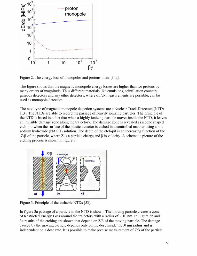
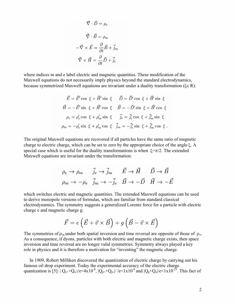
Figure 2. The energy loss of monopoles and protons in air [34a].

The figure shows that the magnetic monopole energy losses are higher than for protons by many orders of magnitude. Thus different materials like emulsions, scintillation counters, gaseous detectors and any other detectors, where dE/dx measurements are possible, can be used as monopole detectors.

The next type of magnetic monopole detection systems are a Nuclear Track Detectors (NTD) [13]. The NTDs are able to record the passage of heavily ionizing particles. The principle of the NTD is based in a fact that when a highly ionizing particle moves inside the NTD, it leaves an invisible damage zone along the trajectory. The damage zone is revealed as a cone shaped etch-pit, when the surface of the plastic detector is etched in a controlled manner using a hot sodium hydroxide (NAOH) solution. The depth of the etch-pit is an increasing function of the Z/β of the particle, where Z is a particle charge and β is velocity. A schematic picture of the etching process is shown in figure 3.

Figure 3. Principle of the etchable NTDs [53]. In figure 3a passage of a particle in the NTD is shown. The moving particle creates a zone of Restricted Energy Loss around the trajectory with a radius of ~10 nm. In Figure 3b and 3c results of the etching are shown that depend on Z/β of the moving particle. The damage caused by the moving particle depends only on the dose inside the10 nm radius and is independent on a dose rate. It is possible to make precise measurement of Z/β of the particle

6

out to large values of Z/β, which is shown in Figure 4.

Figure 4. Comparison of very low β and high β particle-damages in NTDs [53].

ade by 26 keV/u 56Fe ions with

Because of radiation quenching in the dense core region near a monopole trajectory, NTDs is more

he

3. Magnetic monopole search experiments

No magnetic monopole has found in the experiments performed so far. Below we will analyze

]

shown: the accelerator name or location, reaction type, incident particle momentum (energy),

Figure 5. A scanning Electronic Micrograph of etch pits mβ=0.007 [53].

sensitive to energy deposited in the halo by δ rays. After the etching, the NTDs are scanned on electron Micrographs. There are special markers on NTDs, which allow to determine hole position accuracy less than 100 µm in several layers of the NTDs used in the experiments. Tetchable NTDs are calibrated using heavy ion beams (see Figure 5).

accelerator based monopole search experiments, from the first one performed in 1959 [14] up tothe latest published one in 2006 [34] to get an idea of what can be achieved at a RHIC search experiment [55] in comparison to the previous monopole search experiments. A compilation [5of accelerator based experiments is presented in Table 1. In the table following parameters are

7

corresponding center of mass energy, monopole mass limit achieved, cross section limit, value magnetic charge, experimental technique used, year of publication, and references . . In between the first [14] and the last [34] experiments there were many accelerator-b

of

ased periments, which are presented in a table 1. Monopole search was performed practically at all

two

[5].

N Year Ref.

exnew accelerators, having a new energy domain to explore. Below we will consider the firstexperiments at the LBL and at the BNL AGS. Later we will compare experiments within a groupwith best results in cross section limits and mass coverage achieved.

Table II. Compilation of the accelerator based experiments from PDG

Accele- Rator

Reaction Beam Energy

√s GeV Mass limit

Cross Section

MM Charge

TEC

Gev GeV cm^2 LBL pA 3.76 EMUL 1959 14 6.2 <1 1.e-40 1 CERN pA 7.6 <4 CNTR 1961 15a 28.0 <3 1.e-35 AGS pA 30.0 7.86 <3 2.e-40 <2 CNTR 1963 15 CERN pA 28.0 7.6 <3 1.e-40 <2 EMUL 1963 15b IHEP pA 70.0 11.9 <5 1.e-41 EMUL 1972 16 FNAL pA 400 28.3 <13 5.e-42 <24 CNTR 1974 17a ISR pp 60 60 <30 3 1.e-36 < PLAS 1975 25 FNAL pA 400 28.3 <12 5.e-43 <10 INDU 1975 17 FNAL pA 300 24.5 2.e-30 OSPK 1975 17bIHEP pA 70 11.9 <5 1.e-40 <2 CNTR 1976 17c CERN pp 56 56 <30 3 1.e-37 < PLAS 1978 26 CERN pp 63 63 <20 1.e-37 <24 CNTR 1978 17d SLAC e+e- 29 29 <30 4.e-38 <3 PLAS 1982 27 CERN pp 52 52 <20 8.e-36 CNTR 1982 24 CERN e+e- 34 34 10 4.e-38 <6 PLAS 1983 29 CERN pp 540 ,3 540 1.e-31 1 PLAS 1983 18 SLAC e+e- 29 29 3.e-38 <3 PLAS 1984 28 FNAL pap 800 1800 1800 < 3.e-38 >=1 PLAS 1987 18aCLEO e+e- 10.6 4 5 10.6 < 9.e-37 <0.1 CLEO 1987 18bCERN e+e- 50-52 50-52 <24 8.e-37 1 PLAS 1988 18c DESY e+e- 35 35 <17 1.e-38 <1 CNTR 1988 30 KEK e+e- 50-61 50-61 <29 1.e-37 1 PLAS 1989 31 FNAL pp 1800 0 .5 180 <850 2.e-34 >=0 PLAS 1990 23 CERN e+e- 88-94 88-94 <45 3.e-37 1 PLAS 1992 32 CERN e+e- 88-94 88-94 PLAS 1993 33 CERN PbA 160A 17.9 <8.1 1.9e-33 2 >= PLAS 1997 18dAGS AuAu 3.3 .65e-33 =2 11A 4.87 < 0 > PLAS 1997 18dFNAL pap 1800 1800 260-420 7.8e-36 2-6 INDU 2000 19 FNAL 10pap 1800 1800 265-4 0.2e-36 1-6 INDU 2004 20 HERA e+p 300 300 0.5e-37 1-6 INDU 2005 22 FNAL pap 1800 1800 369 0.2e-36 >=1 CNTR 2006 34

8

The first experiment [14] was done at the LBL Bevatron with a proton momentum of 6.2

lene

and

icles.

an

at

he next experiments to search for magnetic monopoles were conducted at BNL AGS and at

ig.6. a) Elevation view of the BNL AGS apparatus; b) Details of counter arrangement;

GeV/c. Nuclear emulsions were used to search for Dirac magnetic monopoles. Different targets were used in the experiment: A 0.005’’ Aluminum, 0.5’ copper and 3mm polyethytargets were placed in the14.2 kilogauss magnetic field alternatively. Emulsions were later placed behind the target to detect magnetic monopole, which would have gained ~ 4 GeV energy, when moving in the magnetic field. It was expected that such monopole would deposit their entire 4 GeV energy in the emulsion, when traversing black paper wrapping1000 µ of emulsion. Monopoles with masses between the π meson and the proton were expected to be detected by these emulsions, which were sensitive to highly ionizing partThe response was checked by observation of a natural α particle background in the emulsion and by observation of α particles and fission fragments from CF252, which had been soaked into several spots of the emulsion. No signal characteristic of monopole passage in the emulsion was found. Different targets used in the experiment used different integrated luminosities. For Aluminum the cross section limit of 2x10-35 cm2 was achieved and forcopper corresponding limit was 1.5x10-37 cm2. A polyethylene target was bombarded by integrated flux of 1017 protons and later placed 2.5 cm from nuclear emulsions and was exposed to a 200 kilo-oersted field. No Monopoles wee found. The authors concluded, ththe cross section is less than 1x10-37 cm2 per nucleon for the production of Dirac Monopoles with binding energy between 3 and 20 eV in polyethylene. TCERN in the early 60s with incident proton momenta of 30.0 and 28.0 GeV/c, respectively.

Fc)Upper end of focusing solenoid [15].

9

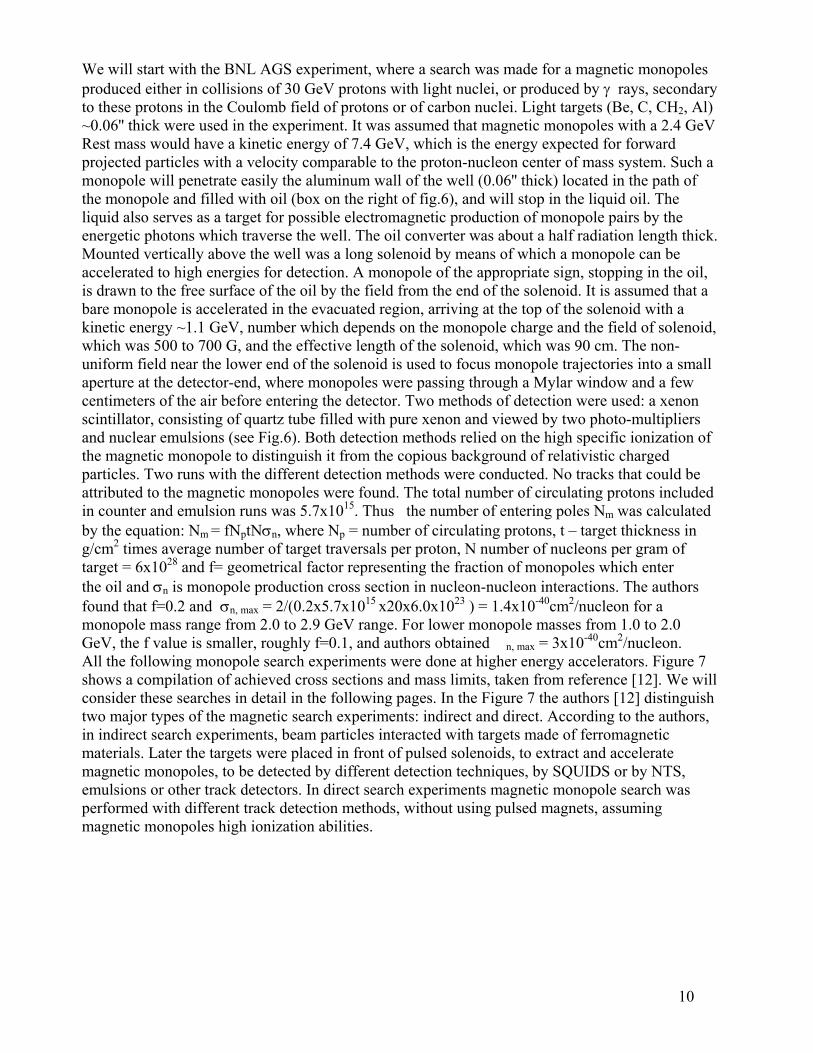
We will start with the BNL AGS experiment, where a search was made for a magnetic monopoles

ick.

s

7 l

,

produced either in collisions of 30 GeV protons with light nuclei, or produced by γ rays, secondary to these protons in the Coulomb field of protons or of carbon nuclei. Light targets (Be, C, CH2, Al) ~0.06'' thick were used in the experiment. It was assumed that magnetic monopoles with a 2.4 GeV Rest mass would have a kinetic energy of 7.4 GeV, which is the energy expected for forward

ch a projected particles with a velocity comparable to the proton-nucleon center of mass system. Sumonopole will penetrate easily the aluminum wall of the well (0.06'' thick) located in the path of the monopole and filled with oil (box on the right of fig.6), and will stop in the liquid oil. The liquid also serves as a target for possible electromagnetic production of monopole pairs by the energetic photons which traverse the well. The oil converter was about a half radiation length thMounted vertically above the well was a long solenoid by means of which a monopole can be accelerated to high energies for detection. A monopole of the appropriate sign, stopping in the oil, is drawn to the free surface of the oil by the field from the end of the solenoid. It is assumed that a bare monopole is accelerated in the evacuated region, arriving at the top of the solenoid with a kinetic energy ~1.1 GeV, number which depends on the monopole charge and the field of solenoid,which was 500 to 700 G, and the effective length of the solenoid, which was 90 cm. The non- uniform field near the lower end of the solenoid is used to focus monopole trajectories into a small aperture at the detector-end, where monopoles were passing through a Mylar window and a few centimeters of the air before entering the detector. Two methods of detection were used: a xenon scintillator, consisting of quartz tube filled with pure xenon and viewed by two photo-multipliers and nuclear emulsions (see Fig.6). Both detection methods relied on the high specific ionization ofthe magnetic monopole to distinguish it from the copious background of relativistic charged particles. Two runs with the different detection methods were conducted. No tracks that could be attributed to the magnetic monopoles were found. The total number of circulating protons includedin counter and emulsion runs was 5.7x1015. Thus the number of entering poles Nm was calculated by the equation: Nm = fNptNσn, where Np = number of circulating protons, t – target thickness in g/cm2 times average number of target traversals per proton, N number of nucleons per gram of

28target = 6x10 and f= geometrical factor representing the fraction of monopoles which enter orthe oil and σn is monopole production cross section in nucleon-nucleon interactions. The auth

15 23 -40 2found that f=0.2 and σn, max = 2/(0.2x5.7x10 x20x6.0x10 ) = 1.4x10 cm /nucleon for a 0 monopole mass range from 2.0 to 2.9 GeV range. For lower monopole masses from 1.0 to 2.

-40 2GeV, the f value is smaller, roughly f=0.1, and authors obtained n, max = 3x10 cm /nucleon. All the following monopole search experiments were done at higher energy accelerators. Figureshows a compilation of achieved cross sections and mass limits, taken from reference [12]. We wilconsider these searches in detail in the following pages. In the Figure 7 the authors [12] distinguish two major types of the magnetic search experiments: indirect and direct. According to the authors, in indirect search experiments, beam particles interacted with targets made of ferromagnetic materials. Later the targets were placed in front of pulsed solenoids, to extract and accelerate magnetic monopoles, to be detected by different detection techniques, by SQUIDS or by NTSemulsions or other track detectors. In direct search experiments magnetic monopole search was performed with different track detection methods, without using pulsed magnets, assuming magnetic monopoles high ionization abilities.

10

Figure 7. Classical Dirac magnetic monopole cross section upper limits vs magnetic moopole mass obtained from direct accelerator searches (solid lines) and indirect searches (dashed lines) [12]. We will consider experiments in chronological order, starting with indirect search experiments. Indirect search experiments showing the lowest cross section limits were obtained in experiments [16], [17] and [18] with mass limits ~10-13 GeV, while other experiments [19,20,33] get higher cross section, but model dependent higher mass coverage.

Figure 8. IHEP magnetic monopole search experimental set-up [16]. The first indirect search, we consider, is the IHEP experiment at the 70 GeV proton synchrotron in Serpukhov, Russia [16]. The proton beam interacted with a ferromagnetic

11

material located inside the vacuum pipe at the edge of the magnet at a distance of 13 cm from the center. At the opposite edge of the magnet two transverse layers of emulsion, 88 mm in diameter were installed. Just behind it was the emulsion chamber of 55x45x30mm3. This system can detect only negative magnetic charges. Knowing the field distribution along z axis, and the properties of ferromagnetic foils, it is possible to calculate the energies, which monopole with a charge g=68.5e will reach on the 26 cm path in the magnet. These energies were found to be 21 GeV, 41 GeV and 58 GeV for experiments with permalloy 79 HM, permalloy 50 H, and permendure, respectively. The monopoles will lose this energy in 1-3 cm of nuclear emulsion. This means that tracks of very high ionization (~5000 more than relativistic proton) might be observed not only inside the two transverse layers of emulsion but also inside those layers of the emulsion chamber for which the trajectory of the monopoles lies in the plane of the field of vision of the microscope. To cover the possibility of an anomalous interaction of the monopoles with material, the irradiated samples were placed in a pulsed magnet with a field of ~800 kG. In this experiment the detector consists of two layers of nuclear emulsion placed near the ferromagnetic foils (see Figure 9). It was assumed that monopole can be trapped in ferromagnetic material with a 100% efficiency. The assumptions were based on publications [16a, 16b]. According to these publications a force binding the monopole to the ferromagnetic medium is: F(Z0) = 2π M0 g ln(R/Z0), where M0 is the saturation magnetization in the solid, R =( g/4π M0)0.5 is the radius of the sphere of saturation surrounding a monopole of strength g in a ferromagnetic medium, Z0 is a cut-off distance, which should not be less than substance inter atomic spacing (1Å). The magnetic field to extract a monopole from the ferromagnetic material is defined as gH0 > F(Z0), or H0 > π M0 ln(g/4πM0 Z2

0). The minimal magnetic field to extract monopole is H = 53 kG for iron and H =54 kG for Permendur. The authors also refer to calculations [16c] of forces of attraction in a monopole-electron and monopole-nucleus systems, if the monopole is a Fermi particle and has an electric dipole moment. Attraction potentials are of 4.6 MeV for aluminum and 5.8 MeV for copper.

Figure 9. Monopole detection set-up: 1.Pulsed magnet; 2.Packet of samples 3.Nuclear emulsion layers [16a].

12

In scanning the emulsion layers no tracks were found crossing both transverse layers with ionization noticeably greater than that of relativistic protons. Then the upper limit for the magnetic monopole production cross section in the reaction p + N -> p + N + g+ + g- is σ(95% CL) < 1.4 x10-43 cm2 if full transparency of the Aluminum target is assumed. If transparency is not assumed and the effective number of nucleons in the nucleus will be A2/3=9 then σ(95% CL) < 4.2 x10-43 cm2 . Next, experiments were done at FermiLab’s proton beam, SLAC’s electron-positron collider and and at the CERN ISR in pp interactions [17]. The most significant irradiation was at Fermilab with 300 GeV protons, producing 2.5x1018 proton-aluminum interactions. The aluminum targets had various lengths from 16.5 cm to 45 cm in different exposures. In order to search monopoles, that could be produced in pairs in the interactions and trapped in the targets, the target material was first ground into thin chips to separate the north and south poles of a pair, using a milling machine, advancing 10µm between successive cuts (the cut was 100µm deep and 12 mm wide). Then, the chips were placed in a hollow rotating sphere to be randomized. They were divided into 30 samples and the magnetic charge of each sample was measured in an electromagnetic detector, schematically shown in Figure 10. The sample was carried several times around a path that traversed a sensing coil. This coil was a part of a superconducting circuit containing two other coils (field coils), each one wound around a sensitive magnetometer (SQUID). If a sample has a none- zero magnetic charge, it will induce a change of current in the superconducting circuit and a change ∆F1 and ∆F2 in the flux measured by SQUIDS 1 and 2. For each SQUID, ∆Φ/Φ0 = νs Np/f, where νs is the ratio of the sample magnetic charge gs to the Dirac unit g0 = e/2α = 137/2 x e (in

Figure 10. Schematic view of the FNAL monopole detector. Samples are moved along the dashed curve labeled as sample path. The superconducting circuit is shown with the sensing coil and field coil connected in series. The magnetometer and auxiliary coil are also shown inside the cryostat [17]. Gaussian units), Φ0 is the flux quantum number of superconductivity (2.07 x 10-7 G cm2), Np is the number of passes through the sensing coil and f is a constant, depending on the various inductance values of the circuit. For SQUID1 f=34, for SQUID2 f= 290. The magnetic charge measurement was done by taking magnetometer readings after 1, 3, 9, 27 and 81 passes. This procedure provided

13

an accuracy of 0.03 for the value of νs. The magnetic charges νs of all the samples were measured to be consistent with zero and incompatible with any value larger than 0.1. From this result a maximum value of Rmax for the ratio of the number of monopole pairs to the number of interactions and the cross sections was been computed at a 95% confidence level. Those calculations were done under the following assumptions: (1) All monopoles are produced with a typical velocity equal to the velocity of the proton-nucleon center of mass system and that they lose ½ of their energy every time they collide with an aluminum nucleus, as do protons at high energy when they collide with nuclei. (2) North and South poles of a pair with large magnetic charge may stop close enough so that the attractive force between them drives them together toward annihilation. Separation due to multiple Coulomb scattering is sufficient to avoid this effect for v<20. For 10<ν<60, large scale Coulomb scattering, and for v>60, nuclear scattering with half energy loss are used to estimate a correction (3). A probability is assumed for the monopoles of a pair to end up in the same chip. (4) If monopoles had charges v<0.1, but there were many of them, the statistical fluctuations would generate some measurable charges for the samples. Therefore the experiment allows computation of upper limits for the density of such monopoles with a reduced sensitivity.

Figure 11. Upper limit (95% confidence level) for monopole pair production cross section in proton-nucleus collisions as a function of magnetic charge. (a) 300 GeV/c protons on aluminum (b) 400 GeV/c protons on aluminum. The solid line curve corresponds to the corrections 1 to 4 described in the text and the dashed curve to corrections 1 and 2 set equal to 1. The dotted curve has been computed using only a 41 cm long target, with a most pessimistic view of the sensitivity of the experiment [17].

14

Next, experiment [18] was performed with the CERN 400 GeV proton beam. The magnetic monopoles were searched for in a series of ferromagnetic collectors of W-Fe powder exposed to the 400 GeV/c proton beam in an experiment at the CERN SPS. The monopole target was made of tungsten-iron (5%) powder compound with 2-3 µm grain size. The material has a density of ~ 12g/cm2. The energy loss of a fast monopole with (n=1) in this material should be 75 GeV/cm. The highly developed ferromagnetic surface in such a target would exclude completely the possibility of bulk diffusion of monopoles and anti-monopoles, thus preventing their annihilation. The W-Fe target was 3 cm in diameter, 31 cm long, and was made of 11 pieces, of which the first five were 1.75 cm long and the last six pieces were 3.5 cm long. They were placed in a metal box (see Figure 12) and were cooled by running water.

Figure 12. Layout of the monopole target in the CERN SPS 400 GeV proton beam experiment [18]. The total exposure was 3x1017 protons on the target. The proton flux was determined by radiochemical methods via thin aluminum foils placed in front of the target. Since the monopole targets were placed after the (anti)neutrino target, it was estimated that they received approximately 1018 pions of ~ 100 GeV average energy. After the exposure the monopole targets were brought to the Kurchatov Institute in Moscow, where monopole extraction was attempted with a strong pulsed magnetic field (see Figure 13).

Figure 13. Sketch of the Kurchatov Institute monopole detector system [18].

15

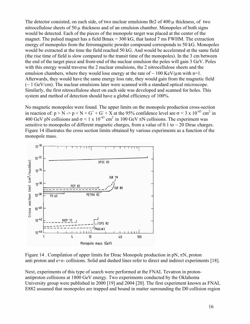
The detector consisted, on each side, of two nuclear emulsions Br2 of 400 µ thickness, of two nitrocellulose sheets of 50 µ thickness and of an emulsion chamber. Monopoles of both signs would be detected. Each of the pieces of the monopole target was placed at the center of the magnet. The pulsed magnet has a field Bmax = 300 kG, that lasted 7 ms FWHM. The extraction energy of monopoles from the ferromagnetic powder compound corresponds to 50 kG. Monopoles would be extracted at the time the field reached 50 kG. And would be accelerated at the same field (the rise time of field is slow compared to the transit time of the monopoles). In the 3 cm between the end of the target piece and front-end of the nuclear emulsion the poles will gain 3 GeV. Poles with this energy would traverse the 2 nuclear emulsions, the 2 nitrocellulose sheets and the emulsion chambers, where they would lose energy at the rate of ~ 100 KeV/µm with n=1. Afterwards, they would have the same energy loss rate, they would gain from the magnetic field (~ 1 GeV/cm). The nuclear emulsions later were scanned with a standard optical microscope. Similarly, the first nitrocellulose sheet on each side was developed and scanned for holes. This system and method of detection should have a global efficiency of 100%. No magnetic monopoles were found. The upper limits on the monopole production cross-section in reaction of: p + N -> p + N + G+ + G- + X at the 95% confidence level are σ < 3 x 10-43 cm2 in 400 GeV pN collisions and σ < 1 x 10-43 cm2 in 100 GeV πN collisions. The experiment was sensitive to monopoles of different magnetic charges, from a value of 0.1 to ~ 20 Dirac charges. Figure 14 illustrates the cross section limits obtained by various experiments as a function of the monopole mass.

Figure 14 . Compilation of upper limits for Dirac Monopole production in pN, πN, proton anti proton and e+e- collisions. Solid and dashed lines refer to direct and indirect experiments [18]. Next, experiments of this type of search were performed at the FNAL Tevatron in proton-antiproton collisions at 1800 GeV energy. Two experiments conducted by the Oklahoma University group were published in 2000 [19] and 2004 [20]. The first experiment known as FNAL E882 assumed that monopoles are trapped and bound in matter surrounding the D0 collision region

16

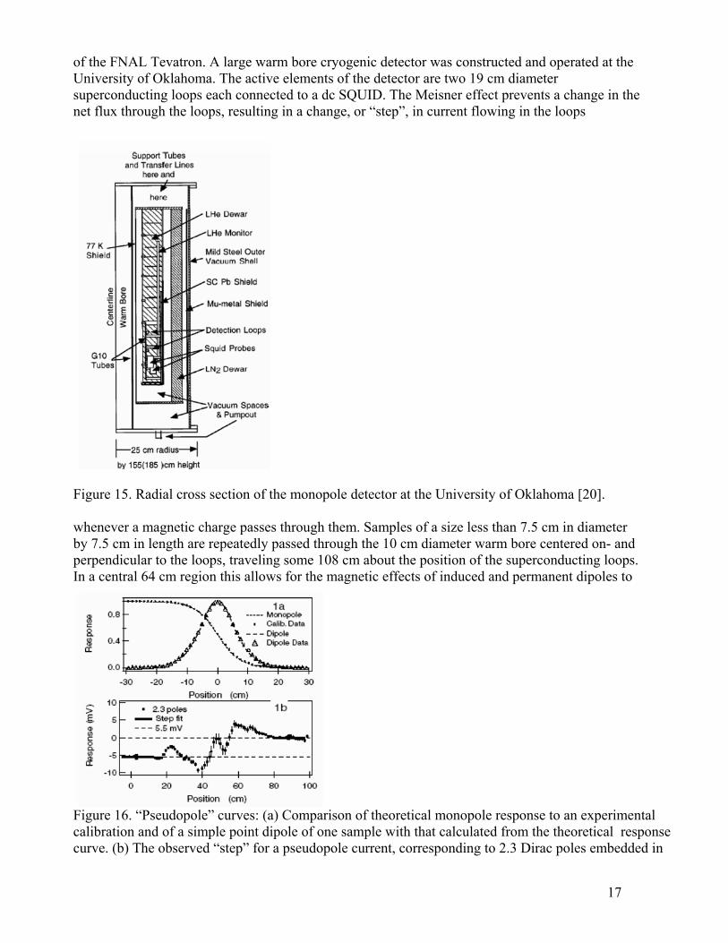
of the FNAL Tevatron. A large warm bore cryogenic detector was constructed and operated at the University of Oklahoma. The active elements of the detector are two 19 cm diameter superconducting loops each connected to a dc SQUID. The Meisner effect prevents a change in the net flux through the loops, resulting in a change, or “step”, in current flowing in the loops

Figure 15. Radial cross section of the monopole detector at the University of Oklahoma [20]. whenever a magnetic charge passes through them. Samples of a size less than 7.5 cm in diameter by 7.5 cm in length are repeatedly passed through the 10 cm diameter warm bore centered on- and perpendicular to the loops, traveling some 108 cm about the position of the superconducting loops. In a central 64 cm region this allows for the magnetic effects of induced and permanent dipoles to

Figure 16. “Pseudopole” curves: (a) Comparison of theoretical monopole response to an experimental calibration and of a simple point dipole of one sample with that calculated from the theoretical response curve. (b) The observed “step” for a pseudopole current, corresponding to 2.3 Dirac poles embedded in

17

an Aluminum sample [19]. return to zero on each up and each down traversals of the sample. The SQUIDS are tuned and their transfer functions measured periodically according to the manufacturer's specifications in order to keep them operating with constant sensitivity. The absolute calibration of the expected signal from the Dirac monopole was made using a “pseudopole”. A long thin magnetic solenoid (1.5 cm diameter by 100 cm length with 4710 turns per meter) carrying a calibrated small current gives a calculable pseudopole at either end. The pseudopole can either be passed through the warm bore of the detector in a way similar to samples or it can be placed in a given position with one end fully extended through the SQUID loops and the solenoid currents repeatedly switched on and off. The shape of observed pseudopole signal is compared to that of theoretical calculations in Figure 16a and the response to a point magnetic dipole is compared to one extracted from the experimental data. Figure 16b shows the step of 5.5 mV (2.3 Dirac poles

Figure 17. Sample spectra. (a) Beryllium sample and (b) Aluminum sample. The observed steps are -0.8 mV in (a) and +0.4 mV in (b). The dipole signals are off scale in the middle regions of the plot [19]. Figure 17 shows examples of the responses from the detector for Be (a) and Al (b) samples “Sbe5P” and “S133Al” respectively. The steps from various samples are plotted in Figure 18. The distribution of steps for data has a mean value of 0.16 mV and spread (sigma) of 0.73 mV. A 90% confidence limits for monopole charges of n = 1 or -1 can be obtained by considering the number samples that are within 1.28 sigma of the n=+/-1 positions, corresponding to samples outside of the central region of +/-1.47 around zero. Eight samples were found outside this central

signal) from a run of a pseudopole embedded in an aluminum sample. There were 222 Al and 6 Be samples from the experiment. All samples were passed through the detector.

18

region, where 10.4 were to be expected from Gaussian error. The 90% confidence upper limit is 4.2 signal events for 8 events observed when ten were expected. In order to be sure that none of the 8

Figure 18. Histogram steps. Vertical dashed lines define the expected positions of signals for various n. The Gaussian curve (dashed) corresponds to 228 measurements having an average value of 0.16 mV and rms 0.73 mV [19]. outlying samples were monopole candidates, the authors measured again the samples that fell within +/-1.47 mV of n = 0. No samples are within a 1.28 sigma of the |n|>2 positions, the closest being 3.08 sigma away from n=-2. The 90% confidence upper limit is 2.4 signal events for zero

s

stopped and that they bind to the magnetic dipole moments of the appropriate uclei 9Be or 27Al and thus are trapped. It is assumed that the interaction of the monopoles with

er nd

y

Ref. [21], that binding should occur for 27Al but not for 9Be (100% natural). However, the

inum, are large and comparable to shell of the monopole the nucleus will

should in general result, even for 9Be. Even an 1 eV would give a lifetime of 10 yr [21].

im that there are a good reasons to believe that ments of nuclei.

a Drell-Yan process: quark-antiquark annihilation to monopole-antimonopole pair via an intermediate high mass virtual photon. The

: oss

ce factor and the velocity dependence of the monopole teraction. The threshold factor is β, the velocity of the monopole in the c.m. system. We take the

interaction factor to be β2, since the Lorentz force for magnetic charges g is F =g(H -vxD). Thus

events observed and zero expected. The upper limit numbers (4.2 and 2.4) are used to derive crossection upper limits for |n|=1 and |n|>=2, respectively. Further it is assumed that monopoles are ranged out andnmagnetic moments of nuclei and electrons can be strong enough to produce bound states undcertain conditions causing the monopoles to be trapped, having a very long lifetime in such boustates [21]. The trapping efficiency is very high. The theoretical modeling that has been done assumes ‘‘rigid’’ extended nuclei with or without repulsive barriers, and some calculations have also been carried out. Electrons can bind to monopoles in a total energy zero state; this probablproduces a small mobile system, which will attach to a nuclear magnetic moment leaving it bound to a fixed nuclear site and permanently trapped. Thus these authors assume that all monopoles bind to appropriate nuclei, i.e., those whose nuclear gyro-magnetic ratio is sufficiently large (anomalous). These models predict, as summarized in(100% natural abundance) and 207Pb (22% natural) estimated binding energies, e.g., 0.5–2.5 MeV for alummodel splitting, so the authors believe that in the presence undergo nuclear rearrangement and binding unreasonably small estimate for the binding energy ofAccording to these assumptions, the authors clastopped monopoles will be trapped by the magnetic mo The monopole production is assumed to derive from

shape of the energy distribution follows from a dimensional argument that is basic to Drell-YanM3ds/dM is dimensionless, where M is the invariant mass of the pair of monopoles. This pp- crsection must include a threshold phase spain

19

the energy shape of dσ/dM is (β/M)3, convoluted with the momentum distributions of the quarkthe colliding proton and antiproton. The total cross section for the monopole production after

s in

d tance, a l ret t the cross section is taken to be n x68.5 larger than the Drell-Yan muon pair cross section, modified by β3, for pp- interactions m ars at an e imit for h

Mass acceptance 0.29 0.015 0.0065 0.13

a second search of magnetic monopoles with rs each exposed to a proton-

easurement was the same as in the les obtained from discarded material

0c] detectors: (1) Be beam pipe and Al kward ‘‘FEM’’ forward

lf of the Al cylinder (‘‘CTC’’ support) from set 2 was reported in a PhD thesis [20a]. All

Here we present a plot of the

Figure 19. Monopole production cross section plot measured in the E882 FNAL experiment [19]. renormalization by n2x68.52 and β3 convolution is shown in Figure 19. Using the total luminosity elivered to D0, 172 +/-8 pb-1, the number limit of monopoles, the (model dependent) accepnd the solid angle coverage, the authors get the pp- cross section limits shown in Table III. Theseimits are of order 100 times better than the Tevatron limit [23] of 200 pb. One can further interphese limits as mass limits using the scaled Drell-Yan cross sections. Here

2 2

easured by CDF [19a] and by D0 [19b]. For such large cross sections a unitarity limit appequivalent n2=9. The authors use the n=1 or 2 scalings for the cases n=1 or 2, and the unitarity ligher n values in converting cross section limits into mass limits. TABLE III. Acceptances, upper cross section limits, and lower mass limits as determined in this reference [19] (at 90% C.L.). Magnetic charge |n| =1 |n| =2 |n| =3 |n| = 6 Sample Al Al Be Be Ω/4π acceptance 0.12 0.12 0.95 0.95

Number of poles <4.2 <2.4 <2.4 <2.4 Upper limit on cross section 0.70 pb 7.8 pb 2.3 pb 0.11 pb Monopole mass limit >295 GeV >260 GeV >325 GeV >420 GeV The University of Oklahoma group performed increased statistics including data from CDF and D0 detectoantiproton luminosity of ~175 pb-1[20]. The method of mprevious experiment [19]. There were three sets of sampfrom the upgrading of the D0 [20b] and CDF [2‘‘extension’’ cylinders from D0, (2) Pb from the forward/bacelectromagnetic calorimeters of CDF, and (3) haCDF sample. Set 1 and 3 were published [20], and three sets are reported according to a final consistent analysis.

20

step functions obtained for 240 Aluminum samples extracted from the CDF experiment (See

periment, with re used for

cross ections and mass limits desired. Each plot determines an upper limit on the number (Nul ) of

e

n +/-8

ion cross

.

t the DESY HERA pipe surrounding the

gnetometer to look for nosity of 62 pb−1 was

agnetic pipe surrounding the H1

aterial of the 21] and so they should remain

pipe was cut into long thin strips UID. Figure22 shows a

agnetic monopoles

the strip through the coil. In contrast, the anent magnetic dipole

Figure 20). Similar step functions were obtained also for other sets of data.

Figure 20. Histogram of the steps from 240 aluminum samples from the CDF exan rms dispersion of 2.7 mV compared to the appropriate Gaussian. These data aobtaining limits for the three magnetic charge values |n| = 2, 3, and 6 [20]. A number of parameters need to be taken from these plots and interpreted to yield the smonopoles of a given magnetic charge (n =1,2,3,6) for each sample set, which in turn determines an upper limit to the corresponding cross section σ < Nul /εeAL, where ε is thefficiency for the chosen signal (a monopole with charge n) to lie outside a cut excluding smaller values of |n|, e is the efficiency of the sample set to cover the solid-angle region choseand to correct for cuts used. L is the total luminosity for the pp- exposure delivered (172pb-1 for D0 and 180 pb-1 +/-5% for CDF). A Drell-Yann model is used for the productsection estimation. Figure 21 shows observed cross sections versus the monopole mass for thedifferent center of mass monopole angular distributions.These cross-section limits are some 250–2500 times smaller and the mass limits are 2–3 times larger than those of reference [23] The last experiment for indirect magnetic monopole search was performed ae+p collider at center of mass energy of 300 GeV [22]. The beaminteraction region in 1995–1997 was investigated using a SQUID mastopped magnetic monopoles. During this time an integrated lumidelivered. For the search reported here the fact is used that heavily ionizing mmonopoles produced in e+p collisions may stop in the beaminteraction point at HERA. The binding energy of monopoles which stop in the mpipe (aluminum in the years 1995–1997) is expected to be large [permanently trapped, provided that they are stable. The beamwhich were each passed through a superconducting coil coupled to a SQschematic diagram illustrating the principle of the method used. Trapped min a strip will cause a persistent current induced in the superconducting coil by the magnetic field of the monopole, after complete passage ofinduced currents from the magnetic fields of the ubiquitous permmoments in the material, which can be pictured as a series of equal and opposite magnetic charges, cancel so that the current due to dipoles returns to zero after passage of the strip.

21

TABLE IV. Alternative interpretations for different production angular distributions of the

monopoles, comparing 1 and 1-cos2 θ to the 1+ cos2 θ limits. Here the acceptance Aa

corresponds to the distribution 1+cos2 θ , and similarly for the cross section and mass limits (all at 90% confidence level). Set n σ ul

+1 pb

mLL+1

(GeV/c2) A0 σ ul

0 (pb)

mLL0

(GeV/c ) A

2-1 σ ul

-1 (pb)

m2

LL-1

(GeV/c ) 1 Al 1 1.2 250 0.024 1.2 240 0.021 1.4 220 1A1 RM 1 0.6 275 0.024 0.6 265 0.021 0.7 245 2Pb 1 9.9 180 0.011 12 165 0.0055 23 135 2Pb RM 1 2.4 225 0.009 2.9 210 0.0045 5.9 175 1 A1 2 2.1 280 0.0068 2.2 270 0.0060 2.5 250 2Pb 2 1.0 305 0.018 0.9 295 0.016 1.1 280 3 A1 2 0.2 365 0.10 0.2 355 0.096 0.2 340 1 Be 3 3.9 285 0.0025 5.6 265 0.0003 47 180 2Pb 3 0.5 350 0.029 0.5 345 0.031 0.5 330 3 Al 3 0.07 420 0.20 0.07 410 0.24 0.06 405 1 Be 6 1.1 330 0.008 1.7 305 0.0008 18 210 3 al 6 0.2 380 0.066 0.2 375 0.082 0.2 370 The beam pipe around the interaction point had a diameter of 9.0 cm and a thickness of 1.7mm in the range −0.3 < z < 0.5m and a diameter of 11.0 cm and thickness 2mm in the range of −0.3 < z < 0.5m and a diameter of 11.0 cm and thickness 2mm in the range 0.5 < z < 2.m. During HERA operations it was immersed in a 1.15 T solenoidal magnetic field which was directed parallel to the beam pipe, along the +z direction. This length of the pipe, covering -0.3 < z < +2.0m, was cut into 45 longitudinal strips each of an average length of 573mm (~ 2 mm was lost at each cut). The central region (−0.3 < z < 0.3m) was cut into 15 long stf width ~ 18 mm, two of which were further divided into 32 short segments varying in len

rips gth

hl which is normally used to measure the residual magnetism in

samples. It consists of three superconductin eter 8.1 cm diam e o i xis par l to nv carri a coil, 2

sv io e d m the transverse coils showed onity t pas f a ca n do-m ole. H ly data the

w us the urements presented by the authors. The sampents were passed through the ma et steps sing a , afte ch

t the rcon g loo e d. T idualete tr ersa sam hroug p mea by ta d ence e

ured c ent and re pas he ings ch sa er eate ral This ow e rep ibility e re to b ied so nd flux s se lin drif uld b ntified a nopo pped i uld g

stent a rep cibl ent ste re how xample of current measu

ofrom 1 to 10 cm. The downstream region (0.3 < z < 2.0m) was divided into 3 longitudinal sections each of which was cut into 10 long strips of ~32 mm width. The long strips and short segments were each passed along the axis of the 2G Enterprises type 760 magnetometer

nograp y Centre, UK. This is a warm bore device with high [22a] at the Southampton Oceaensitivity and a low noise leves

rockits a

g coils of diamed the sata fro

et r,see Fig.

ne w th2) and ly a

alle the co eyor belt werse direct

hich mple (the axial one orientedsmall sensi

in each trantiv

n. Thlibratioo the sage o pseu onop ence on the from

axial coil ere ed in meas les of strips and segm gnetom er in , pau fter each step r whithe curren in supe ductin p was m asure he res persistent current after the compl av l of a ple t h the loo was sured king the iffer in thmeas urr after befo sage. T read for ea mple w e rep d sevetimes. all ed th roduc of th sults e stud that ra om jumpand ba e ts co e ide . Any re l mo le tra n the pipe wo ive aconsi nd rodu e curr p. Figu 23 s s an e rements.

22

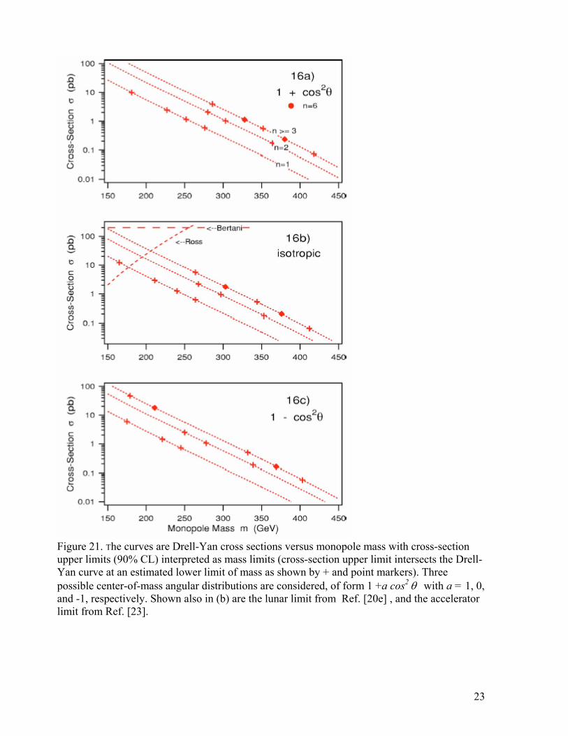
Figure 21. The curves are Drell-Yan cross sections versus monopole mass with cross-section upper limits (90% CL) interpreted as mass limits (cross-section upper limit intersects the Drell-Yan curve at an estimated lower limit of mass as shown by + and point markers). Three possible center-of-mass angular distributions are considered, of form 1 +a cos2 θ with a = 1, 0, and -1, respectively. Shown also in (b) are the lunar limit from Ref. [20e] , and the accelerator limit from Ref. [23].

23

24

ciple of the method. The conveyor belt moved pletely the superconducting coil. At

re the current in the superconducting coil was e for each step was typically 3 s [22].

ved in single readings occurred consistently in ing that no trapped monopole was present.

s section it is necessary to compute the duced which would have been detected. A

model of the production process is therefore needed. Two models were used to compute the acceptance by Monte Carlo technique. In each of these a monopole- antimonopole (MM-) pair was assumed to be produced by a photon-photon interaction. The first model (model A) assumed spin 0 monopole pair production by the elastic process e+p -> e+ MM-p through the interactions of a photon radiated from each, the electron and the proton. The proton was assumed to have the simple dipole form factor 1/(1 + Q2/0.71GeV2), where Q2 is the negative square of the four momentum transferred to the proton. The second model (model B) assumed spin 1/2 monopole pair production by the inelastic process e+p -> e+ MM-X (where X is any state) through a photon-photon fusion interaction with a photon radiated from the electron and one radiated from a quark in the proton. The photon is radiated with a simple distribution given by (1-η)5/η, with η the fraction of the proton’s energy carried by the photon. While the models implement the cinematic correlations in each event, it should be noted that they depend on

igure 23. The measured persistent currents (in units of gD), after passage through the magnetometer, plotted against sample number for the two strips of the central beam pipe which were cut into short segments [22].

Figure 22. The schematic diagram shows the prinin steps of typically 5 cm until the sample traversed comeach step the conveyor belt stopped for 1 s beforead to avoid the effects of eddy currents. The tim It can be seen that none of the fluctuations obserother readings on the same sample show To derive an upper limit on the measured crosacceptance, i.e. the fraction of the monopoles pro

F

perturbation theory and therefore the predicted cross sections are unreliable. Events were generated according to model A using the program CompHEP [22b] and using a dedicated program for model B. The generated final state particles were tracked through the H1 magnetic field to the beam pipe. If the thickness of beam pipe traversed was greater than the calculated range of the monopole in aluminum, it was assumed to stop. In this way the fraction of monopoles, which were detected by stopping in the beam pipe, was computed. Figure 24 shows obtained cross section limits for the two models.

eft) n

in the acceptance computed from the models described above. Here the acceptance is the fraction of the monopole pairs which produce either one or both monopoles which stop in the beam pipe. Figure 24 (left plot) shows the upper limit on the cross section at 95% confidence level for monopoles of strength 1, 2, 3 and 6gD using acceptances determined from model. A Figure 24 (right plot) shows the upper limits determined using the acceptances from model B. Thus, the upper limits on the monopole pair production cross section have been set for monopoles with magnetic charges from 1 to 6gD or more and up to a mass of 140 GeV within the context of the models described. We have discussed above indirect experimental methods of magnetic monopole detection. All these experiments assume that produced magnetic monopoles can stop, be trapped and be bound in the material surrounding a collision region. There are several assumptions made here

del

indirect experimental results. We here also

Figure 24. Upper limits on the cross section, determined within the context of model A (land model B (right), for monopole-antimonopole pair production in e+p collisions as a functioof monopole mass for monopoles of strength gD, 2gD, 3gD and 6gD or more [22]. The failure to observe a monopole candidate means that there is an upper limit of 3 monopole pair events produced at the 95% confidence level. The cross section upper limit is then calculated from this, taking into account the uncertainties in the measured integrated luminosity and in the fraction of the pipe surviving the cutting procedure, and the statistical uncertainty

[21] based on estimated binding energies of ~0.5-2.5 MeV, comparable with a shell mosplitting, achievable when magnetic monopole is trapped in ferromagnetic materials. These

ication [12] claiming that it is difficult to establish the assumptions were criticized in publalidity of the hypotheses made, to interpret the v

25

26

gree with the conclusion made in [12], that it currently seems impossible to check assumptions

23]. ty-two

ere exposed for 4 months, 6 stacks were exposed r 6.5 months and remaining ones were exposed for ~ 2 months. Each stack consists of 4 layers of

CR39, each 1.4 mm thick, and 4 layers of Lexan, 0.35 mm thick, in 4 stacks also included 2 layers of nitrocellulose, 0.3 mm thick. The stacks covered a solid angle ranging between 0.7 to 0.3 of 4π in the different running periods. The first layer of CR39 was etched in a NAOH solution 8N at 80 C0 for 80 to 100 hours. This strong etching procedure reduces the thickness of the sheet from 1.4 mm to about (0.5-0.2) mm. A monopole that traversed a sheet would result in a hole after etching and thus would be easily detectable. The etched CR39 plates were scanned with a stereoscopic microscope type Wild-M4 using low magnification x6 and x40. Only 3 holes were found in the strongly etched sheets. For this case, in order to look for a coincidence, the authors etched the second CR39 sheets of the stack using a more conventional etching technique, in NAOH, 6N, at 60 0C for 30 hours. No tracks were found at the place anticipated from the holes in the first plate. In order to measure the effective threshold of the used CR39 when heavily etched, as well as for normal etching, the authors exposed stacks of CR39 to relativistic sulfur ions of 200 GeV/nucleon at the CERN-SPS (see Figure 25) and to 0.6 GeV/nucleon neon ions at the Bevalac at Berkley. They found a threshold of Z/β=8 for both normal and heavy etching. Thus,

count

% confidence vel) with n>0.5 and mass less than 850 GeV. For the masses smaller than 50 GeV the detection

he

apresented in reference [21]. Now we will consider the direct search experiments presented in Figure 7. We start with the FNAL 1800 GeV center of mass energy proton-antiproton experiment at the FNAL Tevatron [The search was based on the plastic track detector techniques, using CR-39 NTDs. Twenstacks of 7x13 cm2 foils were placed around the 10 cm diameter, 0.16 mm thick, stainless-steel beam pipe at the E0 interaction point. 14 stacks wfo

the efficiency of monopole detection is almost 100% with β > 0.2 and n > 0.5. Taking into acthe integrated luminosity, the solid-angle coverage and the detection efficiency the authors obtained an upper limit of monopole production cross section σ < 2x10-34 cm2 (95leefficiency decreases and the limit increases slightly.

Figure 25. Micro photograph of CR-39 exposed to 200 GeV/nucleon sulfur ions. Holes are due to the sulphur nuclei [23]. The plot of monopole production cross section versus the monopole mass was published in tconference materials of the NATO Advanced Study Institute in 1983 [24] and is shown in Figure 26 corresponding to 5x10-38 cm2 and a mass limit up to 20 GeV.

Figure 26. The 95% confidence level limits on monopole production cross section as a function of monopole mass in the ISR experiment [24]. The next two experiments [25] and [26] continued a search for magnetic monopoles at the CERN ISR complex. In experiment [25] most of the exposure was done at the pp cms energy of 45

plastic sheets were placed around the lastic sheets, each 200 µm thick,

sheets of each stack were of Makrofole-E, and the stack were positioned on supports by means of 3 w tracks from one sheet to another with an

hown in Figure 27 and Figure 28 shows

and 53.2 GeV and also at 62.8 GeV. 12 stacks ofinteraction region I1 of the ISR. Each stack consisted of 10 pwith a surface of (9x12) cm2. The 3rd and 5th

8 others nitrocellulose. The 10 sheets of each pins. This references made it possible to follouncertainty of (20-30) µm. The experimental layout is s

27

Figure 27. Experimental layout of the CEERchamber, D – detector [25].

N ISR experiment. B – beam, V – vacuum

se to

t the surface of the nitrocellulose sheets. The corresponding figure for Makrofol-E is about 107

protons. In the etched plates these fragments yield a general background which shows up as randomly oriented tracks. The background tracks appear only at the two surfaces of the sheet. On the average these tracks do not penetrate farther than 15 µm, and only a few tracks penetrate up to (40-50) µm. Consequently, the scanning was performed by focusing in a region between the two surfaces of the sheet and looking for tracks crossing the whole thickness (see Figure 28). A standard optical microscope with magnification of 26x, 10x was used. No monopoles were found. The authors estimated upper limits at 95% confidence level. The Table V shows obtained limits for the different center-of-mass energies and monopole masses and charges (n=1,2).

Figure 28. Illustration of the scanning procedure of the nitrocellulose sheets. Several background

egion are shown [25]. tracks, a monopole candidate and the scanning r an illustration of the scanning procedure. The solid angle covered by the detector was 3.5 sr. The only material between the crossing region and the first plate was the 0.18 mm stainless

ellulosteel of the vacuum chamber. Tracks were developed by the etching process. The nitroc0sheets were etched in a NAOH 5N solution at 50 C for 60 minutes. The etch was long enough

ensure that the track left by a monopole traversing the 0.2 mm thickness of the sheet would be completely visible for any geometrically possible angle of incidence. A monopole candidate is expected to produce a signal at least in the first nitrocellulose sheet (see Figure 28). The background limit is given by nuclear fragments of low energy with Z>2, produced in the interactions. The measurements show, that 105 protons were needed to produce one visible track a

28

Table V. Upper limits for the production cross section for free monopoles (95% CL) [25]. Ecm GeV 45 0 53.2 62.8 σ (10-36 cm2) mg/mp ε % n =1 5 94 96 98 1.5 10 94 96 98 1.5 20 56 85 94 1.9 25 0 57 90 1.5 30 0 0 61 54 n =2 5 76 84 89 1.8

0 0 40 83 Figure 29 shows a comparison of the obtained results (line 7) to the other experiments.

10 68 79 87 1.9 20 0 23 68 8.8 25

Figure 29. Cross section limit obtained in the ISR experiment [25] (line 7) with other experiments. Another group [26] performed monopole search experiments at the CERN ISR at the energies of 53.2 and 62.8 GeV. A schematic view of the experimental set-up is shown in Figure 30. The exposure took place in the intersection I1 using the superconducting solenoid magnet with a longitudinal field of ~ 1.5 T. The detectors were placed outside the 2 mm thick steel vacuum tank. The geometrical acceptance was 0.5 % of the total angle, near 0 and 180 degrees to the beam. The magnetic field is expected to accelerate monopoles, allowing them cross the steel wall without significant loss. Four stacks of NTD detectors, each containing 4 200µm thick

on supports. sheets, were mounted

29

Figure 30. Schematic experimental set-up of CEanother experiment b) vacuum chamber c) plas

RN ISR experiment [26]. a) detector for tic detectors

Figure 31. Upper limits on the monopole production cross section (95% cl) as a function of mass and charge. The bump at mg/mp=28 GeV arises from the fact that over this limit only the luminosity at 31.4 GeV of the beams can contribute [26]. Each stack consisted of a first sheet of nitrocellulose, most sensitive plastic detector, followed

fol E), less sensitive and by two sheets of nitrocellulose. If a monopole candidate would have been found in the first sheet, the following sheets would have been etched and the track followed from one to the next in order to extract maximum information. Each stack was etched according to the standard technique and scanned with microscopes. No candidates were found during scanning. 95% upper limits were calculated using standard methods and the authors obtained the results shown on Figure 31. The final conclusion was that

by a sheet of polycarbonate (Makro

30

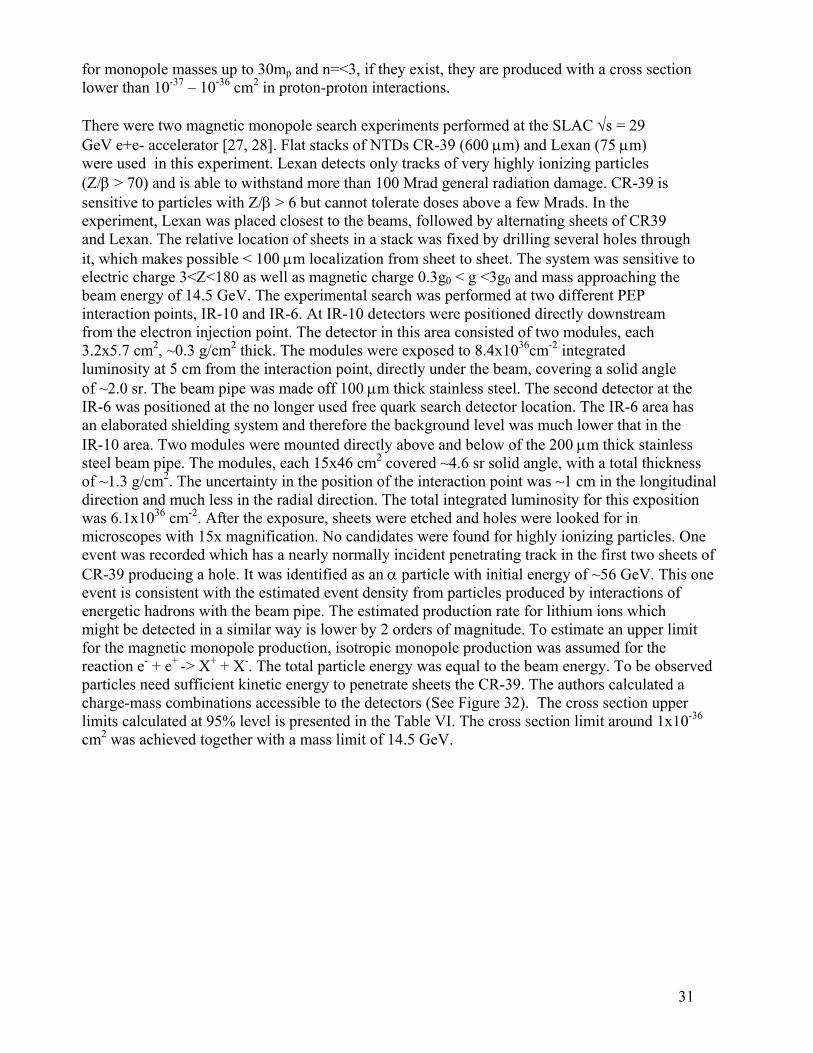
for monopole masses up to 30mp and n=<3, if they exist, they are produced with a cross section lower than 10-37 – 10-36 cm2 in proton-proton interactions. There were two magnetic monopole search experiments performed at the SLAC √s = 29 GeV e+e- accelerator [27, 28]. Flat stacks of NTDs CR-39 (600 µm) and Lexan (75 µm) were used in this experiment. Lexan detects only tracks of very highly ionizing particles (Z/β > 70) and is able to withstand more than 100 Mrad general radiation damage. CR-39 is sensitive to particles with Z/β > 6 but cannot tolerate doses above a few Mrads. In the experiment, Lexan was placed closest to the beams, followed by alternating sheets of CR39 and Lexan. The relative location of sheets in a stack was fixed by drilling several holes through it, which makes possible < 100 µm localization from sheet to sheet. The system was sensitive to electric charge 3<Z<180 as well as magnetic charge 0.3g0 < g <3g0 and mass approaching the beam energy of 14.5 GeV. The experimental search was performed at two different PEP interaction points, IR-10 and IR-6. At IR-10 detectors were positioned directly downstream from the electron injection point. The detector in this area consisted of two modules, each 3.2x5.7 cm2, ~0.3 g/cm2 thick. The modules were exposed to 8.4x1036cm-2 integrated luminosity at 5 cm from the interaction point, directly under the beam, covering a solid angle of ~2.0 sr. The beam pipe was made off 100 µm thick stainless steel. The second detector at the

ed at the no longer used free quark search detector location. The IR-6 area has

inless sr solid angle, with a total thickness

of ~1.3 g/cm2. The uncertainty in the position of the interaction point was ~1 cm in the longitudinal direction and much less in the radial direction. The total integrated luminosity for this exposition was 6.1x1036 cm-2. After the exposure, sheets were etched and holes were looked for in microscopes with 15x magnification. No candidates were found for highly ionizing particles. One event was recorded which has a nearly normally incident penetrating track in the first two sheets of CR-39 producing a hole. It was identified as an α particle with initial energy of ~56 GeV. This one event is consistent with the estimated event density from particles produced by interactions of energetic hadrons with the beam pipe. The estimated production rate for lithium ions which might be detected in a similar way is lower by 2 orders of magnitude. To estimate an upper limit for the magnetic monopole production, isotropic monopole production was assumed for the reaction e- + e+ -> X+ + X-. The total particle energy was equal to the beam energy. To be observed particles need sufficient kinetic energy to penetrate sheets the CR-39. The authors calculated a charge-mass combinations accessible to the detectors (See Figure 32). The cross section upper limits calculated at 95% level is presented in the Table VI. The cross section limit around 1x10-36

2

IR-6 was positionan elaborated shielding system and therefore the background level was much lower that in the IR-10 area. Two modules were mounted directly above and below of the 200 µm thick stasteel beam pipe. The modules, each 15x46 cm2 covered ~4.6

cm was achieved together with a mass limit of 14.5 GeV.

31

Figure 32. The electric charge and mass combination accessible to the PEP detector [27]. TABLE VI. Experimental parameters and upper limits to production cross sections at 95% CL at Eb=14.5 GeV [27]. Combined IR-6 IR-10 limit Integ. Lum. (10-36 cm-2) 6.1 8.4 Pipe thickness (mm) 200 100 Magnetic Monopole Mass limit (GeV) g=g0 13.7 14.0 g=2g0 9.5 11.5 Solid angle (sr) 4.6 2.0 σ (10-36 cm-2) <1.4 <2.3 <0.85 Electric, Z/β > 20 Solid angle (sr) 1.7 1.7 σ (10-36 cm-2) <3.7 <2.7 <1.6 The experiment at the PEP was done later with increased statistic. Figure 33 shows a schematic view of the detector positioned around the beam pipe for the second PEP monopole search experiment. The data for this experiment was taken only at the IR-10 region at a beam energy of 14.5 GeV, which is the same as in the first PEP experiment. Again Lexan and CR-39 plastic sheets were used. The sheets were 80 and 610-725 µm thick respectively and the array was assembled as shown in Figure 33. A set of holes was drilled in the sheets, which allowed individual sheet alignment to ≤100 µm. The total solid angle coverage was 5.0 sr. The sheets were 31.8 cm long and had width of 11.8 and 14 cm, as shown in the Figure 33. The 8th side of the octagonally shaped detector was missing and prior to injection and beam tuning, the detector assembly could be rotated away from the beam pipe into a shielded cave located near the floor level. Thus the detector was better shielded from the background in the IR-10 area, due to the neutrons, produced by the uncaptured e- injection beam. The data for the analysis were taken using two different loadings of

32

Figure 33. Schematic depiction of Lexan and CR-39 plastic detectors used at the PEP monopole

during a 9 month period. Integrated luminosities data analysis method was the same as in e inspected with a microscopes for hole re presented in a Table VII below, including

eters and 95% CL upper limits to production cross 28].

Run1 Run2 Combined

e interaction point and the detector. Kapton was used as a detector, which has the ionization threshold, above which tracks can be detected. This threshold is rather high dE/dx> 4 GeV/g cm-2

search experiment [28]. the detector assembly. Each loading was exposedfor two runs were 30.3x1036 and 150x1036 cm-2. Thethe first PEP experiment. After etching the sheets werobservation. The results at the 95% confidence level athe previous PEP experiment. TABLE VII: Summary of experimental paramsections Eb=14.5 GeV, g0=e/2α=68.5e, Dirac charge [ Ref[27] IR-6 IR-10 IR-10 IR-10 limit Int. Lum(10-36 cm-2) 6.1 8.4 30.3 150 Pipe thickness (µm) 200 100 200 200 Magnetic Mass limit (GeV) g=g0 13.7 14.0 13.7 13.7 Monopole g=2g0 9.5 11.5 9.5 9.5 Solid angle (sr) 4.6 2.0 6.4 6.4 σ (10-36 cm2) <1.4 <2.3 <0.19 <0.039 <0.032 Electric Solid angle (sr) 1.7 1.7 5.0 5.0 Z/β > 20 σ (10-36 cm2) <3.7 <2.7 <1.6 <0.050 <0.041 A search for magnetic monopoles in e+e- collisions was done at √s = 34 GeV of the PETRA storage rings at DESY[29]. The experimenters realized importance of not having material between th

33

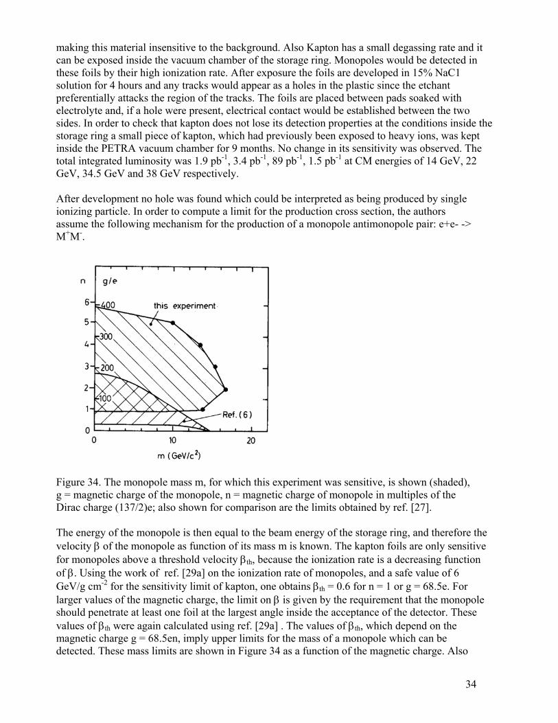
making this material insensitive to the background. Also Kapton has a small degassing rate and it can be exposed inside the vacuum chamber of the storage ring. Monopoles would be detected in these foils by their high ionization rate. After exposure the foils are developed in 15% NaC1 solution for 4 hours and any tracks would appear as a holes in the plastic since the etchant preferentially attacks the region of the tracks. The foils are placed between pads soaked with electrolyte and, if a hole were present, electrical contact would be established between the two sides. In order to check that kapton does not lose its detection properties at the conditions inside the storage ring a small piece of kapton, which had previously been exposed to heavy ions, was kept inside the PETRA vacuum chamber for 9 months. No change in its sensitivity was observed. The total integrated luminosity was 1.9 pb-1, 3.4 pb-1, 89 pb-1, 1.5 pb-1 at CM energies of 14 GeV, 22 GeV, 34.5 GeV and 38 GeV respectively. After development no hole was found which could be interpreted as being produced by single ionizing particle. In order to compute a limit for the production cross section, the authors assume the following mechanism for the production of a monopole antimonopole pair: e+e- -> M+M-.

d), ultiples of the

ref. [27].

ng, and therefore the ils are only sensitive

safe value of 6

rger values of the magnetic charge, the limit on β is given by the requirement that the monopole se

Figure 34. The monopole mass m, for which this experiment was sensitive, is shown (shadeg = magnetic charge of the monopole, n = magnetic charge of monopole in mDirac charge (137/2)e; also shown for comparison are the limits obtained by The energy of the monopole is then equal to the beam energy of the storage rivelocity β of the monopole as function of its mass m is known. The kapton fofor monopoles above a threshold velocity βth, because the ionization rate is a decreasing function of β. Using the work of ref. [29a] on the ionization rate of monopoles, and a GeV/g cm-2 for the sensitivity limit of kapton, one obtains βth = 0.6 for n = 1 or g = 68.5e. For lashould penetrate at least one foil at the largest angle inside the acceptance of the detector. Thevalues of βth were again calculated using ref. [29a] . The values of βth, which depend on the magnetic charge g = 68.5en, imply upper limits for the mass of a monopole which can be detected. These mass limits are shown in Figure 34 as a function of the magnetic charge. Also

34

included in fig.34 are the limits obtained in a similar experiment at SLAC [27]. In order to compute an upper limit for the pair production cross section the authors assumed isotropic production of the monopoles. Using only the luminosity above 34 GeV CM energy, one obtai<4x 10

ns σ ained

and UG-5 detector configuration. The UG-5 is

or three materials [30].

-38 cm-2 (95% CL). This value can be compared with the limit of 0.9 x 10-36 cm-2 obtin a similar experiment at SLAC [27]. A search for highly ionizing particles in e+e- collisions was done at the KEK storage ring TRISTAN [30, 31]. In a first experiment the cms energy was 50 – 52 GeV. In the second experiment the energy was 50 – 60.8 GeV. The detector included two types of etchable solids withwell established response, CR-39 plastic and UG-5 glass. The UG-5, formed into a stack of two

Figure 35. Schematic representation of the CR-39 inside the vacuum while the CR-39 is outside [30]. Table VIII. Detector parameters, sensitivity, and results f

7.5x7.5 cm2 sheets, each 0.9 mm thick, placed 7 cm below the interaction point in vacuum. The placement of the detector inside, rather than outside the vacuum chambers expands

35

significantly the capability to search for particles with short ranges and very high ionization, suas a Dirac monopole with charge 2g

ch

-39

) and the other 6 modules consisted of 4-sheet stacks of 600 µm thick CR-39 (B). The CR-39 stacks were mounted on a movable system, which allows

g ues

No penetrating tracks were found. The 95% confidence upper limit on a cross section for production of highly ionizing particle was calculated taking into account the detection efficiency and the integrated luminosity. Combining the results from the two CR-39 detectors for g = gD, authors found a cross section limit of 8x10-37 cm2 for the most accessible masses, which are 24.1 GeV for a charge gD and 22.0 GeV for charge 2gD. New results were reported from a search for highly ionizing particles at the TRISTAN ring at KEK [31]. The search was sensitive to Dirac monopoles with charge g= 68.5e=gD and g= 2gD

In subsequent running 25.4 pb-1 of integrated luminosity has been accumulated at √s = 55-60.8 GeV. Integrated luminosities at the different run energies for all data accumulated are summarized in Table IX. The luminosity in the experiment was measured using a small-angle Bhabha counter based on lead glass calorimeters. A large-angle counter, based also on lead glass and sensitive to scattering angles of 20°-50°, was used during runs. The ionization produced by magnetic monopoles and the response of track detectors to them is established though calculations analogous to those for electrically charged particles. The ionization rate of magnetically charged particles with velocities β> 0.1 is found to be approximately constant and equal to that of a minimum ionizing particle carrying electric charge of the same magnitude.

or fast particles carrying greater than ~ 0.2gD magnetic charge, solid state track detectors are

ere the same as in the experiment [30]. No andidates were found in the data collected in this experiment. The authors set a 95%

s for dividual detector sectors at each run energy [31].

D, which would lose ~ 10 GeV of energy in the 15 mm thick aluminum beam pipe. Outside the vacuum twelve flat stacks of the more sensitive CRwere deployed in a polyhedral configuration, to increase a detector acceptance. This shape covers a solid angle of ~ 0.9x4π sr (see Fugure35). Six of the detector faces were populated by 3 sheet stacks of 680 µm thick CR-39 (A1to remove them during beam injection and tuning. Standard methods of etching and lookinat sheets via microscopes were implemented. The etching conditions, and scanning techniqtogether with measured upper limits are summarized in the Table VIII.

Fan effective and inexpensive method of detection. The detectors used in the experiment, the method of etching and the stereo microscope used wc Table IX. Integrated luminosity, geometrical acceptance ∆Ω/4π, and cutoff massein

confidence limit on magnetic monopole production cross section. The detection efficiency

36

ε is a function of particle charge, mass and energy and depends on the geometry of the detector, the

th

ed on e

te ss

ce, for monopoles with arge ngD. The total exposure, geometric acceptance and cutoff masses M1c2 and M2c2 for each

rocess by which the particle is resumed to be produced. For Dirac monopoles the most obvious mechanism is annihilation

n of a

not f

h

sheet thickness, the response of the detector as a function of ionization rate, the scanning method used and the beam pipe thickness. A particle satisfying the ionization criterion is detected wiefficiency ~1 if it has sufficient energy to penetrate the beam pipe plus two sheets of detector material. Where the efficiency is equal to the geometric acceptance of 0.86, the σlim establishusing all of the data is 1×10-37 cm2. The overall efficiency for a particle of a given mass depends the energy spectrum of the produced particles. In the absence of specific models of production, thauthors calculate efficiencies and limits as a function of mass for isotropic, exclusive pair production of Dirac monopoles with charge gD and 2gD . The efficiency is calculated via MonCarlo simulation as a function of mass and run energy. The cutoff mass Mn is defined as the maat which the detector efficiency is half the maximum geometric acceptanchdetector sector are compiled in table above. This search is classified as "direct" in that no assumptions have been made about the properties of the monopole aside from the magnitude and magnetic nature of the charge. The significance of the limit is depends on the physical ppand pair production via the electromagnetic interaction. If one assumes a single-photon production process, then the amplitude for pair production is proportional to the magnetic charge. Ignoring higher order effects, one can then formulate a naive pair production cross section for monopoles of mass m, σD(m), by multiplying the cross section for productioµ+ µ− pair with invariant mass greater than 2m by the square of the charge ratio and making a phase space correction: σD(m) = (gD/e)2 x σµµ(>2m) × ( 1-4m2/s). The phase space term had been included in previous report. The quantity RD = σ(m)/σD(m) then be expected to be oorder unity for point-like Dirac monopoles with magnetic charge gD (and ~4, for charge 2gD), at energies above threshold. In e+e – annihilations the µ pair cross section is well approximated by lowest order QED, where they are produced with invariant mass equal to the center of mass energy. In pp of pp- collisions µ pairs are produced with a distribution of invariant mass whicis well measured for pp up to √s = 60 GeV and may be extrapolated to higher energies by scaling. Experimental limit on RD, accumulated over all runs, is shown in Figure 36 together with other previous searches. From this analysis the authors conclude that point-like Dirac

37

Figure 36. Upper limit at 95% confidence on RD = σ( m )/σD ( m ) for isotropic exclusiveproduction of monopole pairs with charge (a) g

e es

t

he 89

rst:

below shows composition of modules in the two runs of the experiment. In each exposed module the two front sheets, closest to the interaction point, were analyzed. Table X. Detector compositions and exposure [32]. Run I II Int. Lum. (nb-1) 30+/-6 30+/-6 CR-39 type A B C D thickness µm 720 1500 730 1500 No. modules 3 9 6 6 In all cases at least one of the two front sheets was etched heavily and scanned rapidly, while others were examined if a track passed the scanning criteria. Holes were located by an ammonia technique [32a] or by microscope inspection at low magnification (16x). To calculate general

D and (b) 2gD . The thick line indicates limit obtained accumulated using all exposures. Both TRISTAN results shown include a phase spaccorrection, as described in the text. Selected limits shown from previous accelerator search[31a] and from cosmic rays [31b] have not been adjusted for phase space. monopoles with mass below 28.8 GeV/c2 are ruled out. Two experiments at the CERN LEP e+e- accelerator were performed by the MODAL [32] and OPAL [33] collaborations. The MODAL experiment was run at √s = 91.1 GeV energy. Thedetector used CR-39 plastic foils covering a 0.86 x 4π sr angle surrounding the I5 interaction poinat LEP. The polyhedral array was supported by a frame which was mounted on a fixed stand. Taluminum vacuum pipe was a thin of 0.5 mm aluminum. Runs were performed at energies √s = – 93 GeV. The integrated luminosity was accumulated at √s = 91.1 GeV and was 60+/-12 nb-1. The 12 detector faces were filled with several types of CR-39 material. The thickness were fi720 µm(Α), second: 1500 µm (Β), third: 730 µm (C). Detector response of all three plastic detectors were calibrated using heavy ions at the Lawerence Berkeley Laboratory. Table X

38

detection efficiency an isotropic magnetic mgD and 2gD. The acceptance and cutoff mass for each dete Table XI. Detector parameters, sensitivity, and re

onopole pair production was simulated with charges ctor is presented in Table XI below.

sults [32].

During the analysis no candidates for highly ionizing particles were found and the upper limit ofproduction cross section of such particles at a 95% confidence level was established: 7x10

the .

opole pair production with a charge g as hes in e+e- collisions. Open symbols are

was done at two energy domains of eV [33b]. The OPAL detector was

range 0.9 gD < g < 3.6 gD , where gD =

the

-35 cm2

The Dirac magnetic monopoles with masses below 44.9 GeV/c2 were ruled out.

Figure 37. Upper limits at 95% CL on magnetic mon

rca function of √s/2 for MODAL and TRISTAN sea-for pp [17], CERN ISR [26] and pp [23] results.

The magnetic monopole search with the OPAL [33] detector

.3 Gthe LEP machine: at LEP1 ~ 90 GeV and at LEP2 ~ 206ensitive to Dirac monopoles with magnetic charge in thes

68.5e. The OPAL detector, is a general purpose set-up with the main task of e+e - interactionsstudies at the LEP collider. Monopole detectors based upon plastic track-etch foils, assembled as three sets of three layers of Lexan, were wound around the OPAL beam pipe. Each of the three layered sets of Lexan was spot welded on a mandrel with exactly the same external diameter as

39

beam pipe. A set of positioning holes was punched through each three layered Lexan set while it was fixed on the mandrel. In addition, scribe marks were placed on the plastic in order that it could be aligned with positioning marks on the beam pipe. Lastly, surveyor's dots

he position of the foils with spect to the beam pipe. In addition, two aluminized Lexan sheets formed the gas seal and the

inner HV foil for the OPAL vertex chamber. The lexan sheets deployed were all 0.125 mm in thickness. The geometric acceptance of this configuration was ~ 0.99 x 4π sr, and its total incremental thickness comprised 0.09% radiation lengths of material. The beam pipe was composed of aluminum and carbon fiber with a total thickness of 1.4 mm. Lexan was deployed in the OPAL experiment from October 1989 to December 1990. In this interval the detector was exposed to 8.67 pb-1 of integrated luminosity at the OPAL intersection region. The first three layers of lexan immediately surrounding the beam pipe were then removed, sensitized by exposure to ultraviolet light [32a] and etched. The passage of such a highly ionizing particle through a dielectric track detector, or plastic track-etch detector, is revealed as a cone shaped etch pit when the surface of the plastic is etched in a controlled manner using hot concentrated sodium. The thickness removed from each surface was 40 m nd 20 µm from the first and second sheets, respectively. The sheets were then

s in the adjacent sheets were examined for tracks, and none were found.

agnetic monopoles of charge gD and 2gD e pair production, and taking into account the magnetic field

in the beam pipe and detector, and etching for Dirac magnetic monopole production

agnetic interaction. If a single-photon y be compared with a lowest-order cross

[30,31], which scales with the cross section ) × ( 1-4m2/s) . Obtained limits can then be

) which would be expected to be of order tic charge g, at energies above threshold.

ost stringent limits from previous earches. The point like cross-section used here is a σµµ

QED= 86.8/E2cm nb, where Ecm is the

entre of mass energy. The 1989-1990 energy scan of the Z° resonance covered the energy

like cross section of 10.4 pb is taken to be e characteristic cross section σ ( m ) . From this analysis, the authors conclude that

section limit is 3 x 10-37 cm2 and mass limit < 45 GeV/c2.

were affixed to allow the CERN surveying team to measure tre

µascanned using an ammonia technique [32a] to locate holes which would be produced by tracks with sufficiently high ionization. Four holes originating from tracks were found in the front sheets, and none were found in the second sheets. The extrapolated track location

The detection efficiency calculation was done for massuming isotropic and exclusivand the geometrical acceptance and energy losses and scanning criteria. The physical mechanismassumed annihilation and pair production via the electromproduction process is assumed, then the limit masection σD(m) for a point like monopole of mass mfor unlike-sign dimuons: σD(m) = (gD/e)2 x σµµ(>2mexpressed as limits on the quantity RD = σ(m)/σD(munity for point like Dirac monopoles with magneObtained limits on Rn are shown in fig. 36 along with the mscrange: 88.23 GeV < Ecm < 94.28 GeV. The corresponding variation in point like cross-sectionis 11.2 pb < σµµ< 9.8 pb: approximately 50% of the luminosity taken with 91.2 GeV <Ecm < 91.3 GeV. The luminosity weighted average pointth D monopoles with mass below 45.0 GeV/c 2 are ruled out. However, it has been speculated that monopoles may have non point like structure, resulting in a suppression of the production cross-section by many orders of magnitude by form factor effects [33a]. This result is able to rule out suppression factors of less than 5 x 104 at 95% confidence. As there are no candidates for highly ionizing elementary particles, the upper limit on the cross section for production of such particles at 95% confidence level is σ < 3/ (εLt) where Lt is the integrated luminosity and ε the detector efficiency. Where the efficiency is equal to the maximum acceptance, and cross

40

The magnetic monopole search was done at the LEP2 accelerator at √s = 203.6 GeV energy

also

[33b]. Figure 38 shows the OPAL detector, which used a cylindrical jet chamber for the magnetic monopole detection. The Jet Chamber (CJ) used for tracking in OPAL, was able

Figure 38 OPAL detector at CERN LEP2 experiment. to measure particle momentum and dE/x as well. Back to back tracks with high energy releasewere searched for in opposite CJ. No corresponding signals were found in data of 63 pb-1 integrated luminosity. Figure 39 shows simulated charge per hit in the OPAL Jet Chamber produced by usual particles (blue histogram) and measured (black points), and a simulation of the signal from magnetic monopoles (pink histogram). Detector simulation was done for efficiency determination. The obtained upper limit on the magnetic monopole production cross section is shown in figure 40. A cross section limit of 5 x 10-39 cm2 was achieved for monopole masses in the 45 - 100 Gev/c2 region.

41

Figure 39. OPAL Jet Chamber signals for simulated magnetic monopoles (pink), standard particles (blue histogram) and data (black points) [33b].

Figure 40. Monopole production cross section limit obtained at the LEP OPAL detector at 2√s = 203.6 GeV energy [33b].

42

The last direct magnetic monopole search experiment was published in 2006 [34]. This search ilab Tevatron

agnetic and

as the z sverse plane. The

er (COT) and the time the solenoid. The coverage of the cylindrical

∼ 1. The COT consists of res. The COT makes position

easurements for

.

cally used to correct on and production of

ore than 500 m ionizing particle (MIP).

he experiment used a highly ionizing particle trigger that requires large light pulses at both nds of a TOF scintillator bar. The trigger was designed to detect monopoles efficiently while

consuming less than 1 Hz of the CDF data acquisition bandwidth. The continuous low rate

uses a 35.7 pb-1 sample of pp- collisions at √s = 1.96 TeV produced by the Fermand collected by the CDF II detector during 2003 using a special trigger. The detector (see Figure 41) consists of a magnetic spectrometer including silicon strip and drift-chamber tracking detectors and a scintillator time-of-flight system, surrounded by electromhadronic calorimeters and muon detectors. CDF uses a superconducting solenoid to produce a 1.4 T magnetic field. The field is parallel to the beam direction, which is taken direction, with θ the azimuthal angle, and r the radial distance in the tranimportant detector components for this search are the central outer track-of-flight (TOF) detector, both positioned inside COT extends from a radius of 40 to 137 cm and to pseudorapidity |η|eight super layers, each containing 12 layers of sense wimeasurements for track reconstruction as well as integrated charge mdetermining a particle’s ionization energy loss dE/dx. The COT is surrounded by 216 TOF scintillator bars, which run parallel to the beam line and form a cylinder of radius 140 cmEach TOF bar is instrumented with a photomultiplier tube (PMT) on each end. The TOF measures both the time and height of PMT pulses; the pulse height is typifor discriminator threshold time slewing. Due to their large ionizatiδ rays, monopoles in scintillator with velocity β > 0.2 are expected to produce mtimes the light in the scintillator as produced by a minimu

Figure 41. Schematic view of the FermiLab CDF experimental set-up. Tevatron CDF set-up with a quadrant cut to expose the d iffe subsystems

Te

43

operation allowed the authors validate the trigger performance for the entire data sample. The electronics response of the TOF was calibrated to account for nonlinearities and channel-to-channel differences. The trigger thresholds of about 30 MIPs are well below the expected response to a monopole and have a negligible effect on the trigger efficiency. In the CDF detector, a monopole is accelerated along the uniform solenoidal magnetic field in aparabola slightly distorted by relativistic effects. Because no other particle mimics this behavior, the TOF acceptance must be estimated from Monte Carlo simulations. The authoextended the GEANT3 simulation [34a] to handle magnetic monopoles, including the

rs

te. e

ector

onopole mass, for tic uncertainty [34].

The authors ficiency summarized

ent [34c].. The cross-ection exclusion limit is shown in Figure 43. The measured limit excludes monopole pair roduction for cross sections greater than 0.2 pb at the 95% confidence level for monopole

implies a mass limit f m > 360 GeV/c at the 95% confidence level. This is currently the best limit from a direct

acceleration by the magnetic field, energy loss, and multiple scattering [34b]. Bremsstrahlung is not simulated as this is a negligible effect for monopoles in the mass range of consider. The TOF acceptance for monopole pairs simulated with GEANT is shown in Figure 42. Light monopoles, accelerated strongly by the magnetic field, tend to be swept out of the detector before reaching the TOF. Heavy monopoles, produced near threshold, suffer the same fate. 13000 events were selected which passed trigger requirements. Detailed analysis of these events doesn't shows a single case that can be considered as a magnetic monopole candidaTherefore the authors reported a limit of the cross section as function of the magnetic monopolmass. The expected number of events N from a process with cross section σ and det

Figure 42. The acceptance of the TOF for monopole pairs, as a function of mDrell-Yan monopole pair production. The band indicates the total systema efficiency with acceptance ε after integrated luminosity L is given by N = Lεσ.calculated the cross-section limit for zero observed events, based on the efin Table XII below and a 6% uncertainty in the luminosity measuremspmasses between 200 and 700 GeV/c2. For the Drell-Yan mechanism, this

2 osearch.

44

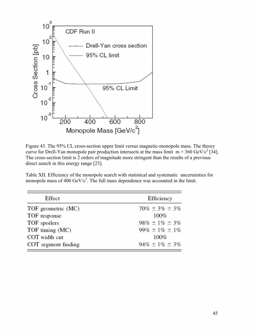
Figure 43. The 95% CL cross-section upper limit versus magnetic-monopole mass. The theory curve for Drell-Yan monopole pair production intersects at the mass limit m > 360 GeV/c2 [34]. The cross-section limit is 2 orders of magnitude more stringent than the results of a previous direct search in this energy range [23]. Table XII. Efficiency of the monopole search with statistical and systematic uncertainties for monopole mass of 400 GeV/c2. The full mass dependence was accounted in the limit.

45

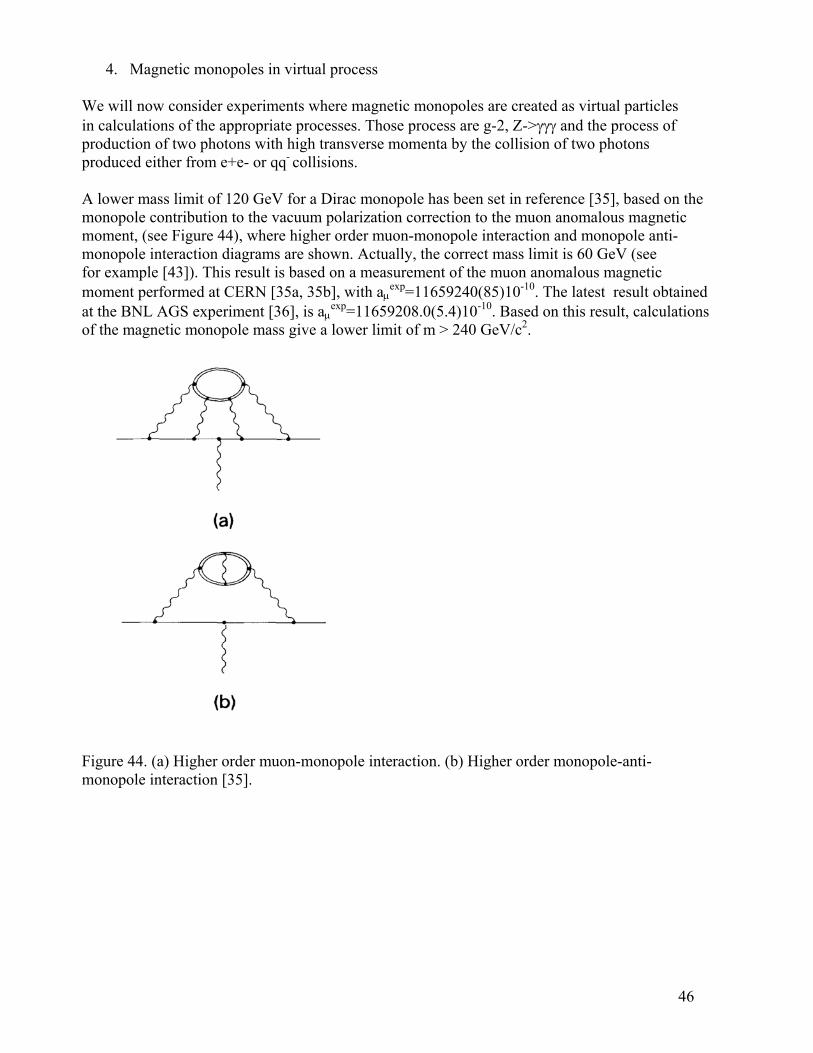
4. Magnetic monopoles in virtual process We will now consider experiments where magnetic monopoles are created as virtual particles in calculations of the appropriate processes. Those process are g-2, Z->γγγ and the process of production of two photons with high transverse momenta by the collision of two photons produced either from e+e- or qq- collisions. A lower mass limit of 120 GeV for a Dirac monopole has been set in reference [35], based on the monopole contribution to the vacuum polarization correction to the muon anomalous magnetic moment, (see Figure 44), where higher order muon-monopole interaction and monopole anti-monopole interaction diagrams are shown. Actually, the correct mass limit is 60 GeV (see for example [43]). This result is based on a measurement of the muon anomalous magnetic moment performed at CERN [35a, 35b], with aµ

exp=11659240(85)10-10. The latest result obtained at the BNL AGS experiment [36], is aµ

exp=11659208.0(5.4)10-10. Based on this result, calculations of the magnetic monopole mass give a lower limit of m > 240 GeV/c2.

Figure 44. (a) Higher order muon-monopole interaction. (b) Higher order monopole-anti-monopole interaction [35].

46

Figure 45. Z-production in e+e- annidual photon vertices (denoted by vertex on the electron line. (b) A dual viceQED background [38]. The experiment L3 at the LEP CERN [37] searThis process was not found, but 95% CL limprocess in references [38, 43] (see Figure around 400 GeV/c2. Another virtual process where monopoles are in1982 [39] and Ginzburg and Schiconsidered of two photons with high transverproduced either from e+e- or qq- monopoles could re-scatter pairs diagram as shown in Figure 46.

hilation and monopole-induced Z->3γ decay. (a) With the a heavy dot) hooked to the monopole line and the standard

versa. (c) A higher-order correction to (a). (d) The

ched for Z decaying directly into three photons. it of 1x10-5 was obtained. The calculations of this

45), rule out the magnetic monopole mass up to

volved was studied by Ginzburg and Panfil in ller in 1999 [40, 41] (see Figure 46). The production was

se momenta by the collision of two photons collisions. A virtual heavy point like Dirac magnetic of nearly real photons into the final state via a box monopole

Figure 46. Feynman diagram for γγ production via a virtual monopole loop [41]. Based on this theoretical scheme, an experimental limit was given by the D0 collaboration [42],

47

which sets the following bounds on the monopole mass M: M/2|m'GeV for S = ½ and > 1580 GeV for S = 1, where S is the spin of the mthe magnetic charge quantization number.

| > 610 GeV for S =0, > 870 onopole, and m' = eg is

considered above rely on the Feynman diagram shown in figure 47. If e particle in the loop is an ordinary electrically charged electron, this process is well known.

, ],

nd -F2/16π +α2/360 x 1/m4 x 1/(4π)2 x [4(F2)2 + 7(F*F)2] where m is the mass

f the particle in the loop. The Lagrangian for a spin-0 and spin-1 charged particle in the loop is ield

in the =

ticle e

.0306 and 3.50 for spin 0, spin 1/2, and spin 1 particles in the the photon scattering through a

nce of the string, which renders perturbation ted by A. De Rujula [38] and Ginzburg [40]

ry of Maxwell equation with respect to the gnetic charge brings in Maxwell equation

tions, as for charges and currents too. For ion loop graph in the presence of zero-

fields. Since the Euler–Heisenberg Lagrangian is means we obtain the low energy

the equation for the QED cross section by

It is critical to emphasize that the Euler–Heisenberg Lagrangian is an effective Lagrangian

er, it ecomes unreliable if radiative corrections are large. The same has been noted in another

Figure 47. The light-by-light scattering graph for either an electron or a monopole loop [43]. The three processes we thIf, further, the photons involved are of very low momentum compared with mass of the electronthen the result may be simply derived from the well-known Euler-Heisenberg Lagrangian [44-46which for a spin-1/2 charged-particle loop in the presence of weak homogeneous electric amagnetic fields is: L = ogiven by a similar formula, which is derived in references [46, 47]. Given this homogeneous-feffective Lagrangian, it is a simple matter to derive the cross section for the γγ−>γγ process low energy limit. Explicit results for the differential cross section are given in [43]: ds/dΩ 139/32400 π2 x α4 x ω6/m8 x (3 + cos2 θ)2 and the total cross section for a spin-1/2 charged parin the loop is σ = 973/10125 π x α4 x ω6/m8 ; ω/m<<1, s = 4w2. The numerical coefficients in thtotal cross section are 0.00187, 0loop, respectively. The applicability of the above calculations ofmonopole loop seems impossible because of the existetheory meaningless. This box diagram was calculaappealing to duality, which is the dual symmettransformations E->M, M->-E. The introduction of masymmetry with respect to the E -> B, B -> -E transformalow energy γ processes it is enough to calculate the fermenergy photons, in the presence of static, constant invariant under the duality substitution on the fields alone, thiscross section σγγ−>γγ through the monopole loop fromthe substitution e -> g, or α −> α g = 137 m'. 2|m'| = 1, 2, 3, .

for calculations at the one fermion loop level for low energy, i.e. ω/m<<1. Howevb

48

context in other works [48-52]. The internal radiative correction to the box diagram have been computed by [50] and [51,52] in QED. In the O(α2) term in the expansion of the Euler Heisenberg Lagrangian (see above), the coefficients of (F2)2 and (F*F)2 terms are multiplied

and (1+1315/252 x α/π + O(α2)), respectively. The corrections α −> αg.

a problem arising with the unitarity bound. The [42] seem incorrect. If higher order effects are

ts quoted are inconsistent. If one takes the cross section 8 and makes the duality substitution, one obtains σγγ−>γγ =

8 x 1/M2 x (ω/m)6 for the low energy light-by-light presence of a monopole loop (M is the monopole mass). If the

l wave of angular momentum J, the cross (2J +1)/s ~ 3π/s, at J~1. Comparing this with the cross

ection given above, one obtains the following inequality for the cross section to be consistent ith unitarity: M/ω > 6|m'|. At the same time the limits quoted by D0 for the monopole mass

by (1 + 40/9 x α/π + O(α2)) become meaningless when we replace In Ref. [43] it was emphasized that there is results given in [40, 41] and used in the analysis involved, it seems that the mass limigiven by σ = 973/10125π x α4 x ω6/m973/10125π x α4 x ω6/m8 = 1.08 x 107 x m'scattering cross section in the cross section were dominated by a single partiasection would be bounded by σ < πsware less than this: M/2|m'| > 870 GeV, spin ½, because, at best, a minimum estimate is <ω>

300 GeV, so the theory cannot sensibly be applied below a monopolemass of about 1 TeV. ~(Note that changing the value of J in the unitarity limits has very little effect on the bound sincean 8th root is taken: replacing J by 50 reduces the limit only by 50%.) Similar remarks can be directed towards the limits in reference [38]. The author, however, notes the “perilous use of a perturbative expansion in g”. However, although he writes down the correct vertex, he does not, in fact, use it, instead appealing to duality, and even so author admittedly omits enormous radiative corrections of O(αg) without any justification other than what is believed, is a specious reference to the use of effective Lagrangian techniques for these processes. The Table XIII below summarizes obtained magnetic monopole mass limits in the processes where monopoles are considered as virtual particles. Experimental results [36, 37] and [42] are excluding monopole masses below 610 GeV, 870 GeV and 1580 GeV depending on spin of the magnetic monopole. Nevertheless, all above mentioned processes are suffering from a problem of higher order corrections, and additional experimental verifications of these results are required. Table XIII. Magnetic monopole mass limits in g-2, Z -> γγγ and High Pt γ’s measured in different experiments [36, 37 and 42]. Process Mass Limit, GeV Reference g-2 > 240 35, 36, 43 Z -> γγγ > 400 37, 38, 43 High Pt γ > 610 S=0 39 – 43 High Pt γ > 870 S=1/2 39 – 43 High Pt γ > 1580 S=1 39 - 43

49

5. Future magnetic monopole search experiments Now we will consider future magnetic monopole search experiments. We will start with the MOEDAL experiment [53] at the CERN LHC accelerator complex [54]. CERN LHC – a large

4 TeV in the proton-proton mode and will ccelerate Lead heavy Ions to √s = 5.5 TeV energy per nucleon. The proton-proton expected

ves

igure 48. The LHCb experiment with MOEDAL detector at the CERN LHC accelerator [53].

. e.

), with a total thickness ~5mm (see Figure 49). Alignment of the monopole track

hadron collider - will operate an energy of √s = 1aluminosity will reach 1 x 10-34 cm2 s-1 and there is an LHC upgrade project with tenfold luminosity increase. With this unprecedent energy and luminosity scale there is a big challenge to look for the magnetic monopoles to cover higher mass regions of a few TeV. Figure 48 gi

F a schematic view of the LHCb experimental set-up, where the MOEDAL experiment will runThe MOEDAL detector consists of NTDs, which will be mounted on a light aluminum framIt will contain five plastic sheets per triangle element (Lexan – CR-39 – Lexan – CR-39 - CR-39 – Lexan

50

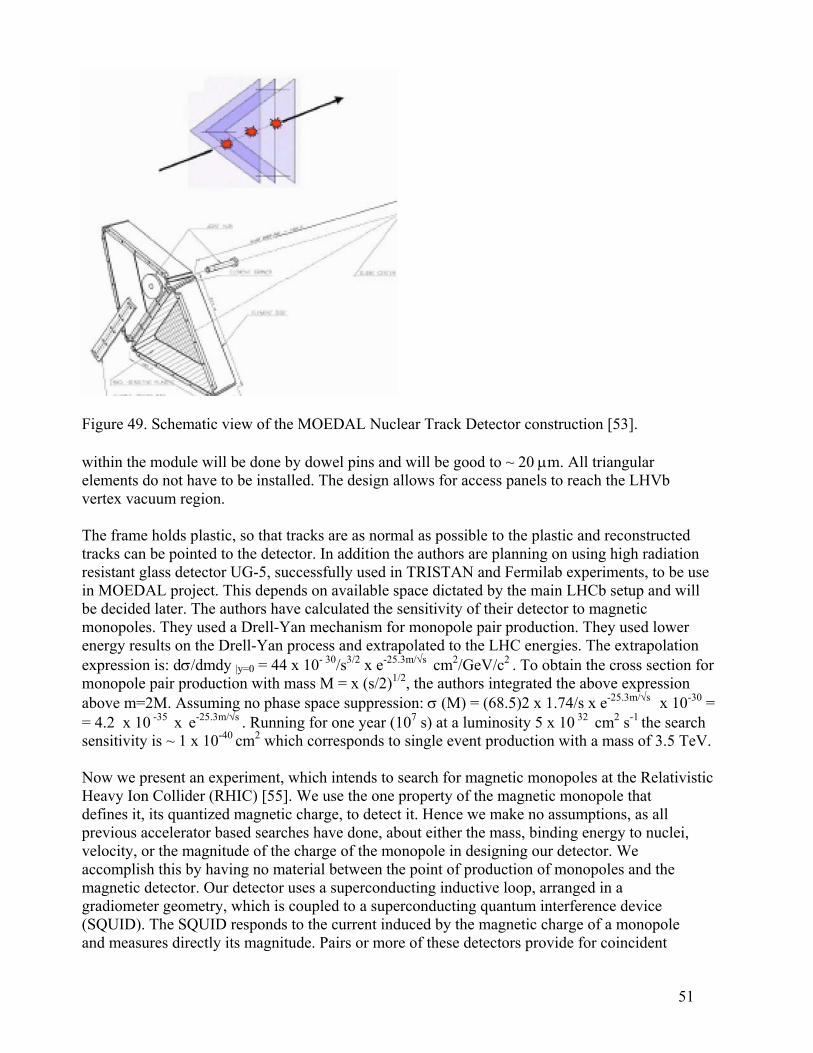
construction [53].

µm. All triangular

to reach the LHVb

plastic and reconstructed

acks can be pointed to the detector. In addition the authors are planning on using high radiation se

MOEDAL project. This depends on available space dictated by the main LHCb setup and will e decided later. The authors have calculated the sensitivity of their detector to magnetic

n

tion for

bove m=2M. Assuming no phase space suppression: σ (M) = (68.5)2 x 1.74/s x e-25.3m/ s x 10-30 = = 4.2 x 10 -35 x e-25.3m/√s . Running for one year (107 s) at a luminosity 5 x 10 32 cm2 s-1 the search sensitivity is ~ 1 x 10-40 cm2 which corresponds to single event production with a mass of 3.5 TeV.

Now we present an experiment, which intends to search for magnetic monopoles at the Relativistic Heavy Ion Collider (RHIC) [55]. We use the one property of the magnetic monopole that defines it, its quantized magnetic charge, to detect it. Hence we make no assumptions, as all previous accelerator based searches have done, about either the mass, binding energy to nuclei, velocity, or the magnitude of the charge of the monopole in designing our detector. We accomplish this by having no material between the point of production of monopoles and the magnetic detector. Our detector uses a superconducting inductive loop, arranged in a gradiometer geometry, which is coupled to a superconducting quantum interference device (SQUID). The SQUID responds to the current induced by the magnetic charge of a monopole and measures directly its magnitude. Pairs or more of these detectors provide for coincident

Figure 49. Schematic view of the MOEDAL Nuclear Track Detector

within the module will be done by dowel pins and will be good to ~ 20 elements do not have to be installed. The design allows for access panelsvertex vacuum region.

The frame holds plastic, so that tracks are as normal as possible to the trresistant glass detector UG-5, successfully used in TRISTAN and Fermilab experiments, to be uinbmonopoles. They used a Drell-Yan mechanism for monopole pair production. They used lowerenergy results on the Drell-Yan process and extrapolated to the LHC energies. The extrapolatioexpression is: dσ/dmdy |y=0 = 44 x 10- 30/s3/2 x e-25.3m/√s cm2/GeV/c2 . To obtain the cross secmonopole pair production with mass M = x (s/2)1/2, the authors integrated the above expression

√a

51

detection schemes to rule out spurious magneticplaced behind the gradiometers and is used to moproduced by collisions. Figure 50 shows the dete

signals. In addition, a silicon detector is nitor and measure the energy loss of particles ctor which will be installed at the RHIC.

he RHIC has two operation modes: Heavy Ions, mainly Gold-Gold (Au-Au) and polarized

d

Figure 50. Cross Section of the monopole detector cryostat [55]. Tprotons at the energy 100 GeV/nucleon and 100 GeV, respectively. The following integrated luminosities are expected at the RHIC collider [56] in the years 2007 and 2008: (see Table XIV). Table XIV: Maximum luminosities that can be reached after a sufficiently long running period.

All numbers are given for operation at an energy of 100 GeV/n. The RHIC also aims to run at √s = 500 GeV polarized pp interactions. The luminosities quoteabove are planned to be enhance to the following values: Lstore avg = 8×1026 cm-2s-1 for Au-Au at 100 GeV/n (4× design) Lstore avg = 6×1031 cm-2s-1 for p-p at 100 GeV,

52

Lstore avg = 1.5×1032 cm-2s-1 for p-p at 250 GeV (16× design) both with 70% polarization

Figure 51 Minimum and maximum projected integrated luminosity for Au-Au collisions [56].

for p-p collisions [56].

inosities has a geometrical efficiency

onopole production with this efficiency and also with maximum efficiency (after detector upgrade), which we consider to be 50%, using the expected RHIC luminosities.

Figure 52 Minimum and maximum projected integrated luminosity Figure 51 and 52 show expected minimum and maximum projected integrated lumat RHIC for AuAu and pp interactions, respectively. Our detector of 0.5%. We have calculated upper limits for magnetic m

53

The cross section limit at 95% confidence level, when no magnetic monopole candidates is expressed as σ< 3.0/(ε Ldt), where ε is the detection efficiency and Ldt the integrated

pp integrated used in our calculations the

r the cross section in pp

agnetic minosities

its for 0.5 efficiencies with 3

e are

nopole at RHIC and

σ (pb)

luminosity. According to Figure 52 the projected minimum of delivered luminosity is ~180 pb-1 and the projected maximum is 380 pb-1. Weaverage between those two values which is 280 pb-1. The limit fointeractions that can be obtained with 250 GeV energy option is based on following numbers: luminosity of 1.5 x 1032 cm-2s-1, one year (107 s) RHIC operation. This will correspond to : 1.5 x 1032 cm-2s-1 x 107s = 1500 pb-1. The Table XV below presents expected mmonopole production cross section limits with different efficiencies and integrated luin pp interactions at RHIC. We also included LHC expected limexpected LHC luminosities: 5 x 1032 cm-2s-1 (At the beginning of the LHC operation), 1 x 1034 cm-2s-1 (normal LHC operation) and 1 x 1035 cm-2s-1 (LHC Upgrade plan). Wassuming one year (107 s) operation for each luminosity.

Table XV. Expected production cross section limits for the magnetic moLHC in pp interactions.

Energy Ldt ( pb-1) ε σ (pb) 100 280 0.005 2.1 100 280 0.5 0.021 250 1500 0.005 0.4 250 1500 0.5 0.004 14000 1500 0.5 0.0012 1.2 x 10-39 cm2

1400 1500 0.5 0.00006 6.0 x 10-41 cm2

1400 1500 0.5 0.00006 6.0 x 10-42 cm2

We can also estimate the same numbers for the Auand at LHC (Lead-Lead at 5.5 TeV/nucleon). For RHIC we assume6×1026 cm-2s-1 (average between maximum and minimum values see Filuminositiy of 1 x 1027 cm-2s-1 [57] and one year operation time. heavy ions we use the expected Z4 enhancement [58] of the crinteractions. This enhancement in case of AuAu is 794 = 3.895 x 107

. Table XVI. Expected production cross section limits for the maAuAu and LHC in PbPb interactions.

Au interactions at RHIC (100 GeV/nucleon) d a projected luminosity of

gure 51) and for LHC, a To calculate these numbers for

oss sections in heavy ion and for PbPb 824 = 4.521 x107

gnetic monopole at RHIC

-1 Energy Ldt ( pb ) ε σ (pb) σ (pb) 100 6 0.005 100000 100 6 0.5 1000 100 6 0.005 0.0026 2.6 x 10 cm-39 2

100 6 0.5 0.000026 2.6 x 10 cm-41 2

5500 10 0.5 0.00013 1.3 x 10-41 cm2

We should point out that in the case of heavy ion collisions with Z4 enhancement, the obtained ross sections rise rapidly with the monopole mass, because the inc

which are responsible for mtensity of the γγ interactions,

onopole production, falls rapidly with the produced particle mass [59].

54

Figures 53 and 54 shows γγ luminosity functions [59a], with the a number of γγ interadependent on the mass of the produced system for RHIC AuAu interactions at 100 GeVnucleon and for LHC PbPb interactions at 5.5 TeV per nucleon, respectively.

ctions per

e 53. The lum function at R r Gold-Gold ctions [59a].

e 54. The lum sity function at L

ll return to th onopole production cross section in collisionscuss the monopole production in pp interactions. A ioned ear

Figur inosity HIC fo intera

Figur ino HC for Lead-Lead interactions [59a]. We wi

ill die m heavy io

s we mentn s. Now we

lier in wour overview, due to the high coupling constant of the magnetic monopole, there is no way

55

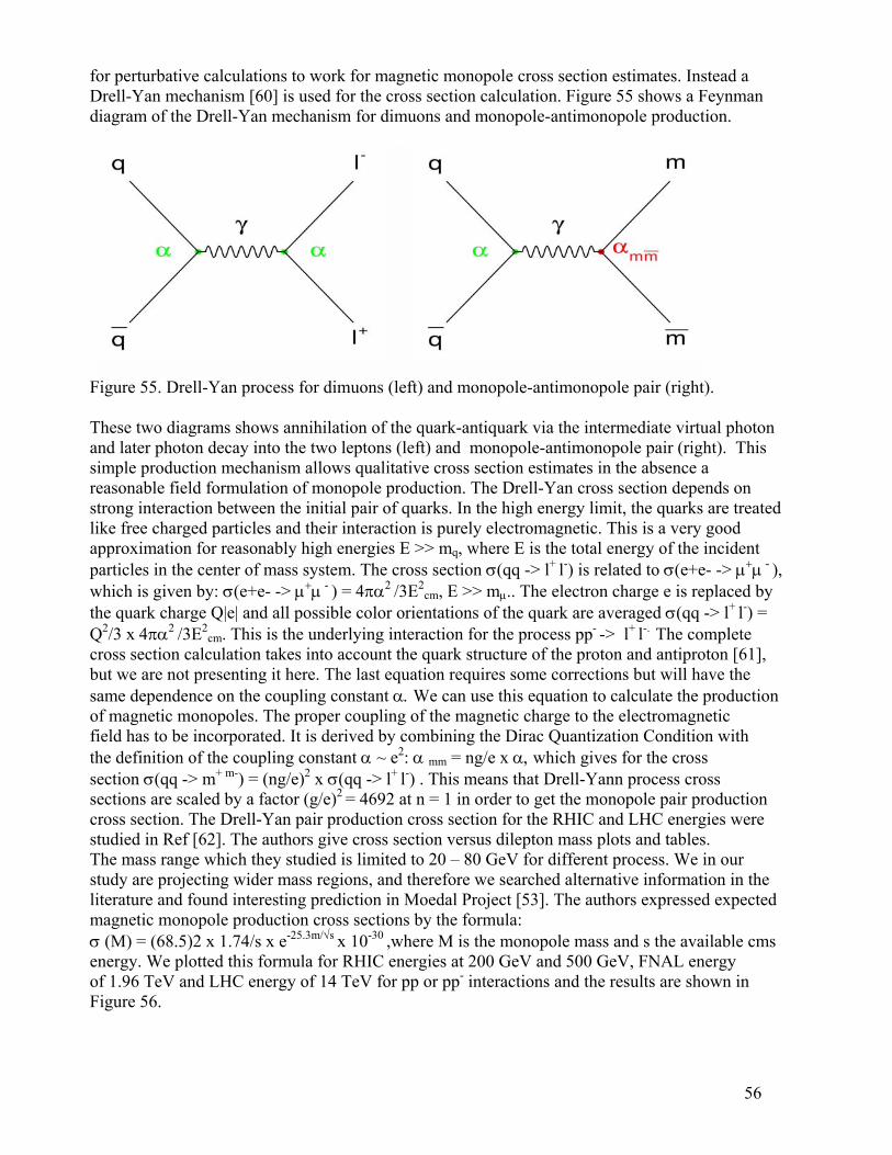
for perturbative calculations to work for magnetic monopole cross section estimates. Instead a n

onopole-antimonopole pair (right).

termediate virtual photon onopole-antimonopole pair (right). This

imple production mechanism allows qualitative cross section estimates in the absence a ion depends on

strong interaction between the initial pair of quarks. In the high energy limit, the quarks are treated agnetic. This is a very good

l energy of the incident ) is related to σ(e+e- -> µ+µ - ),

charge e is replaced by e quark are averaged σ(qq -> l+ l-) =

- -> l+ l-. The complete the proton and antiproton [61], corrections but will have the

calculate the production gnetic charge to the electromagnetic

combining the Dirac Quantization Condition with ives for the cross

eans that Drell-Yann process cross get the monopole pair production

section for the RHIC and LHC energies were ass plots and tables.

he mass range which they studied is limited to 20 – 80 GeV for different process. We in our information in the expressed expected

agnetic monopole production cross sections by the formula: -25.3m/√s -30 le cms

y in

Drell-Yan mechanism [60] is used for the cross section calculation. Figure 55 shows a Feynmadiagram of the Drell-Yan mechanism for dimuons and monopole-antimonopole production.

Figure 55. Drell-Yan process for dimuons (left) and m These two diagrams shows annihilation of the quark-antiquark via the inand later photon decay into the two leptons (left) and msreasonable field formulation of monopole production. The Drell-Yan cross sect

like free charged particles and their interaction is purely electromapproximation for reasonably high energies E >> mq, where E is the totaparticles in the center of mass system. The cross section σ(qq -> l+ l-

which is given by: σ(e+e- -> µ+µ - ) = 4πα2 /3E2cm, E >> mµ.. The electron

the quark charge Q|e| and all possible color orientations of thQ2/3 x 4πα2 /3E2

cm. This is the underlying interaction for the process ppcross section calculation takes into account the quark structure of but we are not presenting it here. The last equation requires somesame dependence on the coupling constant α. We can use this equation toof magnetic monopoles. The proper coupling of the mafield has to be incorporated. It is derived by the definition of the coupling constant α ~ e2: α mm = ng/e x α, which gsection σ(qq -> m+ m-) = (ng/e)2 x σ(qq -> l+ l-) . This msections are scaled by a factor (g/e)2 = 4692 at n = 1 in order to cross section. The Drell-Yan pair production cross studied in Ref [62]. The authors give cross section versus dilepton mTstudy are projecting wider mass regions, and therefore we searched alternativeiterature and found interesting prediction in Moedal Project [53]. The authorsl

mσ (M) = (68.5)2 x 1.74/s x e x 10 ,where M is the monopole mass and s the availab

energenergy. We plotted this formula for RHIC energies at 200 GeV and 500 GeV, FNAL- nd the results areof 1.96 TeV and LHC energy of 14 TeV for pp or pp interactions a shown

Figure 56.

56

Figure 56. Drell-Yan cross section versus mass for magnetic monopoles for RHIC energies of 200 GeV and 500 GeV, FNAL energy of 1.96 GeV and LHC energy of 14 GeV. In Figure 56 the dark blue curve corresponds to the Drell-Yan production cross section versus thmonopole mass for the RHIC energy of 200 GeV, the light blue for RHIC 500 GeV, the black curve for FNAL energy of 1.96 GeV and the red curve for LHC energy of 14 TeV. The mass interval for which we are plotting the curves is between 1 GeV 10 TeV. We find excellent agreement with the Drell-Yan curve for the mass interval of 200 to 600 GeV (see Figure 43) published by the authors of the FNAL CDF experiment [34]. This curve is presented on the Figure 56 in pink color. The above mentioned formula fits very well with the FNAL data [34]. The Moedal Project estimates their expected performance based on that curve. After having such curvefor each energy domain, one can compare the obtained cross section limits with the Drell-Yan

e

s

y)

0 GeV

his

mechanism. Figure 57 shows such a comparison for RHIC energies of 200 Gev and 500 GeV (blue and black curve respectively. The lines correspond to the calculations performed above for 200 GeV

for the detector efficiencand 500 GeV energies for two efficiencies: 0.005 (current Project value and 0.5 – efficiency which might be achievable in case of detector upgrade. The lines for 20are in red and for 500 Gev in blue. For 200 GeV a theoretical curve is crossed at 50 GeV/c2 monopole mass when efficiency is 0.005 and at 70 GeV/c2 when the efficiency is 0.5. This means

-36 2 ε=0 ole up tothat at the cross section limit of 2.1 x 10 cm ( .005) we would see at least 1 Monopmass 50 GeV (and more if the magnetic monopole mass is lower). For the ( ε=0.5) efficiency t

-36 2limit goes up to the 70 GeV for the cross section limit of 2.1 x 10 cm . In case of 500 GeV energy the corresponding limits are 110 and 160 GeV with the efficiencies of 0.005 and 0.5 and

-37 2 -39 2cross sections 4 x 10 cm and 4 x 10 cm ,respectively.

57

Figure 57. Drell-Yan cross section curves for pp interactions at RHIC 200 GeV, 500 GeV, FNAL 1.96 GeV and LHC 14 TeV. Figure 58 shows same plot as Figure 57 for the pp interactions at the LHC energy of 14 TeVred curve corresponds to the predicted Drell Yan process cross sections and the three lines arecalculated cross sections for the detector efficiency of 0.5 and three expected LHC luminosities of 5 x 10

. The our

tion)

.

igure 59 shows similar plots as above Figure 57 and 58, but for RHIC energies of 100 fied by

ction

32 cm-2s-1 (At the beginning of the LHC operation), 1 x 1034 cm-2s-1 (normal LHC operaand 1 x 1035 cm-2s-1 (LHC Upgrade plan). With the LHC normal operation mode we would be able to see one magnetic monopole of 4 TeV mass with a production cross section of 6.0 x 10-42 cm2

FGeV/nucleon in gold gold interactions. Predicted curve of the Drell-Yann process was modia factor of 231 taking into account the number collisions in Au+Au interactions predicted in Ref [62]. We plotted expected cross sections the same way as we did before. Corresponding cross section limits are at the 1.0 x 10-31 cm2 and 1.0 x 10-33 cm2 level. If we take into account the Z4 enhancement of the production cross section we mentioned above and also the luminosity funfor RHIC (see figure 53), we will have two curves for the two detection efficiencies – a black curve for efficiency=0.005 and blue curve for efficiency = 0.5.

58

Figure 58. Drell-Yan cross section curves for LHC at 14 TeV and corresponding predicted cross sections in pp interactions.

Figure 59. Drell-Yan cross section curves for RHIC at 100 GeV/nucleon energy and corresponding predicted cross sections in AuAu interactions.

59

Figure 60. Drell-Yan cross section curves for LHC at 5.5 TeV/nucleon energy and corresponding

nteractions.

curve is a Drell-Yan 4

cm2 could be and 1 x 10-39 cm2 ,

agnetic monopole rent experiments we

IC in pp interactions at 500 GeV ), red line, and also expected cross

s (pink curve). nt with 0.5 efficiency can reach

nts and mass coverage up to ~250

2.

conclusion we would like to thank Drs. A. Baltz, D. Kharzeev and W. Marciano, of BNL vy

predicted cross sections in PbPb i Figure 60 shows similar plots for the expected Drell-Yan Process at LHC energies for the PbPb interactions. The corresponding modification factor was calculated based on results provided in Ref. [63] and [64]. Here only the 0.5 efficiency was considered. The bluecurve, the red line corresponds to the expected cross section, and the black curve shows the Zenhancement of the production cross section. The cross section limit of 6 x 10-34

achieved. For the γγ interactions cross sections ranges between 1 x 10-40 cm2

and reach 1 x 10-37 cm2 at 100 GeV. Figure 61 shows again a plot which was presented on Figure 7, a classical Dirac mcross section upper limits versus magnetic monopole mass obtained in diffediscussed in this article. We added expected cross sections at RHcenter of mass energy for one efficiency: 0.5 ( σ ~ 4 x 10-39 cm2

section in AuAu interaction with the Z4 enhancement of the heavy ion interactionExpected RHIC result for 250 GeV energy proton beam experimea limit which is at the level or better than direct search experimeGeV/c2. Same time in the AuAu interactions monopole production cross section can be achieved better or compatible with direct search experiments in the mass region up to 5 GeV/c Infor fruitful discussions and Dr. A. Baltz for calculation γγ luminosity functions for heaion interactions at RHIC (AuAu) and LHC (PbPb) energies.

60

Figure 61. Classical Dirac magnetic monopole cross section upper limits versus magnetic monopole mass obtained from direct accelerator searches (solid lines) and indirect searches (dashed lines) with RHIC projected cross sections.

61

References [1] Pierre de Maricourt, On the Magnet, letter to Siger de Foucaucourt, (1269). In The Letter of Petrus Peregrinus on the Magnet, New York, 1904. McGraw-Hill. Translated by Brother Arnold. [2] P. Curie, On the possible existence of magnetic conductivity and free magnetism. Seances Soc. Phys. (Paris), 76 (1894). [3] P.L.M. Dirac, Proc. Roy. Soc. A133, 60 (1934). [4] J. C. Maxwell "A Treatise on Electricity and Magnetism", Oxford Classic Text in Physical

Sciences (1873) [5] S. Eidelman et al. (PDG Collab.), Phys. Lett. B 592, 33, 67 (2004)

[6] L.J. Schwinger, Phys. Rev. D12, 3105 (1975) [7] G. 't Hooft, Nucl. Phys. B 79, 276 (1974). [8] M. Polyakov, JETP Letters 20, 430 (1974). [9] K.R. Gienes, E. Dudas and T. Gherghetta Phys. Rev. B 436, 55 (1998). [10] V.A. Rubakov, UFN 171, 913 (2001)[in Russian]. [11] T. Banks et al., Phys. Lett. B212, 45 (1988) [12] G. Giacomelli and L. Patrizi, hep-ex/0506014 and hep-ex/0302011 [13] S. Manzoor et al., e-Print Archive: physics/0611278 [14] H. Bradner and and W. M.Isbell, Phys. Rev. 114, 603 (1959)

(1963) 6] I.I. Gurevich . et al., Phys. Lett. 38B, 549 (1972) 6a] I.I. Gurevich et al., Phys. Lett., 31B, 394 (1970) 6b] E. Goto et al., Phys. Rev. 132, 387 (1963) 6c] E. Amaldi et al., CERN 63-13 (preprint) 1963 7] P.H. Eberhard et al., Phys. Rev.D11, 3099 (1975) 7a] R.A. Carrigan et al., Phys. Rev.D11, 3867 (1974) 7b] D.L. Burke et al., Phys. Lett. 60B, 113 (1975) 7c] V.P. Zrelov et al., Phys. Cz. Jour. Phys., B26, 1306 (1976) 7d] R.A. Carrigan et al., Phys. Rev.D17, 1754 (1978) 8] J.M. Barkov et al., CERN/EP83-194 (preprint) (1983) 8a] P.B.. Price et al., Phys.Rev.Lett., 59, 2523 (1987) 8b] T. Gentile et al., Phys. Rev. D, 35, 1081 (1987) 8c] K. Kinoshita et al., Phys. Rev. Lett., 60, 1610(1988) 8d] Y.D. He., Phys. Rev. Lett, 79, 3134 (1997) 9] G.R. Kalbfleisch. et al., Phys. Rev. Lett. 85, 5292 (2000) 9a] F. Abe et al., Phys. Rev. D 49, R1 (1994) 9b] B. Abbott et al., Phys. Rev. Lett. 82, 4769 (1999). 0] G.R. Kalbfleisch. et al., Phys. Rev. D.69 (2004)

W. Luo, Ph.D. thesis, University of Oklahoma, 2002, UMI-30-56946 (AAT 3056946) 0b] S. Abachi et al., Nucl. Instrum. MethodsPhys. Res. A 338, 185 (1994). 0c] F. Bedeachi et al., Nucl. Instrum. Methods Phys. Res. A 268,50 (1988) 0d] R.R. Ross, P.H. Eberhard, L.W. Alvarez, and R.D. Watt, Phys.Rev. D 8, 698 (1973)

[15] E.M.Purcel et al, Phys. Rev.129, 2326 (1963) [15a] M. Fidecaro et al,Il Nuovo Cim., XXII, 657, (1961) [15b] E. Amaldi et al,Il Nuovo Cim., XXVIII, 773, [1[1[1[1[1[1[1[1[1[1[1[1[1[1[1[1[1[2[20a][2[2[2

62

[21] L.Gamberg, G.R.Kalbfleisch, K.A.Milton, Found.Phys, 30,543 (2000) 2] A. Aktas et al., The European Physics Journal, C 41, 133 (2005) 2a] URL: http://www.2genterprises.com 2b] A. Pukhov et al., arXiv:hep-ph/9908288

et al, Europhys. Lett. 12, 613 (1990) 4] M.J Price., in Monopole ’83edited by J.L. Stone, NATOAdvanced Study

, Letter Al NuovoCimento 23, 357 (1978)

. D29, 1524 (1984)

, 2342 (1982)

(1989) .P. Strauss, Phys. Rev.D 8, 3717 (1973); d P.B. Price, Phys.Rev. D29, 1524 (1984);

, 465 (1983) R.D. Watt, Phys. Rev. D 8, 698 (1973)

alifornia Press,

02 (1982)

s., Sect. A 545, 503 (2005).

Physics, 80, 441 (1981). (2006)

0 (1982) 3 (1998)

6 (1999)

ew York: Addison-Wesley,

[2[2[2[23] M. Bertani[2 InstituteSeries B, Physics, Vol. 111,Plenum, New York, 1983,p.621] [25] G. Giacomelli. et al, Il NuovoCimento28, 212 (1975) [26] M. Hoffmann et al[27] K. Kinoshita et al, Phy. Rev. Lett. 48, 77 (1982) [28] D. Frybergerg et al., Phy. Rev[29] P. Musset et al., Phy. Lett. 128B, 333 (1983) [29a] S.P. Ahlen, Phys. Rev. D17, 229 (1978); S. P. Ahlen and K. Kinoshita, Phys. Rev. D26[30] K. Kinoshita et al., Phy. Rev. Lett. 60, 1610 (1988) [31] K. Kinoshita et al., Phy. Lett. B, 228 , 543[31a] R.A. Carrigan Jr., F.A. Nezrick and B D. Fryberger, T. Coan, K. Kinoshita an B. Aubert, P. Musset, M. Pricc and J.P. Vialle, Phys. Lett.B 120[ 31b] R.R. Ross, P.H. Eberhard, L.W. Alvarez and[32] K. Kinoshita.et al., Phy. Rev. D46, R881 (1992)

niversity of C[32a] R.L. Fleischer Et al., Nuclear Tracks in Solid (U Berkeley, (1975)

3) [33] J.L. Pinfold et al., Phys. Lett. B, 316, 407 (199[33a] A.K. Drukier and S. Nussinov, Phys. Rev. Lett. 49, 1[33b] G. Giacomelli, Talk at the University of Bologna (2006)

2006)[34] A. Abulencia et al., Phys. Rev. Lett. 96, 201801 ([34a] G. Bauer et al., Nucl. Instrum. Methods Phys. Re[34b] S. P. Ahlen, Phys. Rev. D 17, 229 (1978) [35] Graf S et al, Physics Letters, 262B, 463 (1991) [35a] A.I. Studenkin. Sov. J. Part. Nucl. 21, 259 (1990) [35b] E. Picasso NATO Advanced Study Institute, Dr. B,

03-1[36] G.W. Bennett Et al., Physics review, D, 73, 0720[37] M. Acciarri et al Phys. Lett. B 345 609 (1995) [38] A. De Rujula Nuclear Physics, B435 257 (1995) [39] I.F. Ginzburg and S.L. Panfil Sov. J. Nucl. Phys. 36 85

–60[40] I.F. Ginzburg and A. Schiller Phys. Rev. D 57 659901[41] I.F. Ginzburg and A. Schiller Phys. Rev. D 60 075

[42] B. Abbott et al., Phys. Rev. Lett. 81 524 (1998) 2006) [43] K.A. Milton Rep. Prog. Phys. 69 1637–1711 (

[44] W. Heisenberg W and H.Z. Euler Phys. 98 714–32 (1936) 36) [45] V. Weisskopf, Mat. Fys. Medd 14 no.6 (19

[46] J. Schwinger Phys. Rev. 82 664(1951) (N[47] J. Schwinger Particles, Sources, and Fields vol 2

republished by Perseus Books) (1973) [48] M. Bordag and Lindig J. Phys. Rev. D 58 045003 (1998) [49] M. Bordag and Robaschik D. Ann. Phys. (N.Y.) 165 192 (1985) [50] V.I. Ritus, Pisma Zh. Eksp. Teor. Fiz. 69 1517–36 (1975);

63

Sov. Phys.—JETP 42 774 (1975) [51] M. Reuter Schmidt M.G. and Schubert C Ann. Phys. (N.Y.) 259 313–65 (1997)

13 289–300 (1997); 42 (1997)

dal

[52] D. Fliegner et al., Theor. Math. Phys. 1 Fiegner D.et al., Theor. Math. Phys. 113 14[53] J.L Pinfold et al., http://moedal.web.cern.ch/moe[54] http://lhc.web.cern.ch/lhc/ [55] http://www.bnl.gov/npp/docs/pac0906/chaudhari_Monopole-RHIC-PAC.pdf

ections.pdf_JJowett_Oct2006_v2.pdf

(1998)

introduction to Quantum Field theory, Reading, MA:

95)

[56] http://www.agsrhichome.bnl.gov/RHIC/Runs/RhicProj[57] J. Jowett, http://paf.web.cern.ch/paf/Presentations/HI_in_LHC[58]G. Baur, e-Print Archive: hep-ph/0112239 (2001) [59] A.J. Baltz and M. Strikman, Phys.Rev. D, 57, 548 [59a] A.J. Baltz, private communication. [60] I.R. Kenyont, Rep. Prog. Phys., Vol. 45, 1982. [61] M.E. Peskin, D.V. Schroder, An Perseus Books (1995) [62] S. Gavin et al., Int.J.Mod.Phys.A10:2961-2998, (19[63] D. Kharzeev et al., nucl-th/0012025, (2000) [64] D. Kharzeev et al., Nuclear Physics A 747, 609 (2005)

64