Accelerating Simulation of Stiff Nonlinear Systems using Continuous-Time EchoState Networks

Ranjan Anantharaman1, Yingbo Ma2, Shashi Gowda1,Chris Laughman3, Viral B. Shah2, Alan Edelman1, Chris Rackauckas1,2

1Massachusetts Institute of Technology2Julia Computing

3Mitsubishi Electric Research Laboratories

Abstract

Modern design, control, and optimization often require mul-tiple expensive simulations of highly nonlinear stiff models.These costs can be amortized by training a cheap surrogateof the full model, which can then be used repeatedly. Herewe present a general data-driven method, the continuous-time echo state network (CTESN), for generating surrogatesof nonlinear ordinary differential equations with dynamics atwidely separated timescales. We empirically demonstrate theability to accelerate a physically motivated scalable model ofa heating system by 98x while maintaining relative error ofwithin 0.2 %. We showcase the ability for this surrogate to ac-curately handle highly stiff systems which have been shownto cause training failures with common surrogate methodssuch as Physics-Informed Neural Networks (PINNs), LongShort Term Memory (LSTM) networks, and discrete echostate networks (ESN). We show that our model captures fasttransients as well as slow dynamics, while demonstrating thatfixed time step machine learning techniques are unable to ad-equately capture the multi-rate behavior. Together this pro-vides compelling evidence for the ability of CTESN surro-gates to predict and accelerate highly stiff dynamical systemswhich are unable to be directly handled by previous scientificmachine learning techniques.

IntroductionStiff nonlinear systems of ordinary differential equationsare widely prevalent throughout science and engineering(Wanner and Hairer 1996; Shampine and Gear 1979) andare characterized by dynamics with widely separated timescales. These systems require highly stable numerical meth-ods to use non-vanishing step-sizes reliably (Gear 1971),and also tend to be computationally expensive to solve. Evenwith state-of-the-art simulation techniques, design, control,and optimisation of these systems remains intractable inmany realistic engineering applications (Benner, Gugercin,and Willcox 2015). To address these challenges, researchershave focused on techniques to obtain an approximation to asystem (called a “surrogate”) whose forward simulation timeis relatively inexpensive while maintaining reasonable accu-racy (Willard et al. 2020; Ratnaswamy et al. 2019; Zhanget al. 2020; Kim et al. 2020; van de Plassche et al. 2020).

Copyright © 2021for this paper by its authors. Use permitted underCreative Commons License Attribution 4.0 International (CC BY4.0)

A popular class of traditional surrogatization techniques isprojection based model order reduction, such as the properorthogonal decomposition (POD) (Benner, Gugercin, andWillcox 2015). This method computes “snapshots” of thetrajectory and uses the singular value decomposition of thelinearization in order to construct a basis of a subspace of thesnapshot space, and the model is remade with a change ofbasis. However, if the system is very nonlinear, the computa-tional complexity of this linearization-based reduced modelcan be almost as high as the original model. One way toovercome this difficulty is through empirical interpolationmethods (Nguyen et al. 2014). Other methods to producesurrogates generally utilize the structural information knownabout highly regular systems like partial differential equa-tion discretizations (Frangos et al. 2010).

Many of these methods require a scientist to actively makechoices about the approximations being performed to thesystem. In contrast, the data-driven approaches like Physics-Informed Neural Networks (PINNs)(Raissi, Perdikaris, andKarniadakis 2019) and Long Short Term Memory (LSTM)networks (Chattopadhyay, Hassanzadeh, and Subramanian2020) have gained popularity due to their apparent appli-cability to “all” ordinary and partial differential equationsin a single automated form. However, numerical stiffness(Soderlind, Jay, and Calvo 2015) and multiscale dynamicsrepresent an additional challenge. Highly stiff differentialequations can lead to gradient pathologies that make com-mon surrogate techniques like PINNs hard to train (Wang,Teng, and Perdikaris 2020).

A classic way to create surrogates for stiff systems isto simply eliminate the stiffness. The computational singu-lar perturbation (CSP) method (Hadjinicolaou and Gous-sis 1998) has been shown to decompose chemical reactionequations into fast and slow modes. The fast modes arethen eliminated, resulting in a non-stiff system. Another op-tion is to perform problem-specific variable transformations(Qian et al. 2020; Kramer and Willcox 2019) to a formmore suited to model order reduction by traditional meth-ods. These transformations are often problem specific andrequire a scientist’s intervention at the equation level. Re-cent studies on PINNs have demonstrated that such variableelimination may be required to handle highly stiff equationsbecause the stiffness leads to ill-conditioned optimizationproblems. For example, on the classic Robertson’s equations

arX

iv:2

010.

0400

4v6

[cs

.LG

] 2

4 M

ar 2

021

A B

CD

E

Figure 1: Prediction of each surrogate on the Robertson’s equations Shown in each figure is the result of the data-drivenalgorithm’s prediction at p = [0.04, 3×107, 1×104], a parameter set not in the training data. Ground truth, obtained by solvingthe ODE using the Rosenbrock23 solver with absolute tolerance of 10−6, is in blue. The PINN was trained using a 3-layermulti-layer perceptron with the ADAM optimizer for 300,000 epochs with minibatching, and its prediction is in red. Both theESN and CTESN were trained with a reservoir size of 3000 on a parameter space of [0.036, 0.044]× [2.7× 107, 3.3× 107]×[9× 103, 1.1× 104], from which 1000 sets of parameters were sampled using Sobol sampling. The predictions of the CTSENare generated by the radial basis function prediction of Wout(p) and are shown in green. Predictions from the ESN are in purple.The LSTM predictions, in gold, are generated by a network with 3 hidden LSTM layers and an output dense layer, after trainingfor 2000 epochs. (A) A timeseries plot of the y1(t) predictions. (B) The absolute error of the surrogate predictions on y1(t).(C) A timeseries plot of the y2(t) predictions. (D) The absolute error of the surrogate predictions on y2(t). (E) The result ofy1(t) + y2(t) + y3(t) over time. By construction this quantity’s theoretical value is 1 over the timeseries.

(ROBER) (Robertson 1976) and Pollution model (POLLU)(Verwer 1994) stiff test problems it was shown that directtraining of PINNs failed, requiring the authors to performa quasi-steady state (QSS) assumption in order for accurateprediction to occur (Ji et al. 2020). However, many chem-ical reaction systems require transient activations to prop-erly arrive at the overarching dynamics, making the QSS as-sumption only applicable to a subset of dynamical systems(Henry and Martin 2016; Flach and Schnell 2006; Eilert-sen and Schnell 2020; Turanyi, Tomlin, and Pilling 1993;Schuster and Schuster 1989; Thomas, Straube, and Grima2011). Thus while demonstrating promising results on diffi-cult equations, training on the QSS-approximated equationsrequires specific chemical reaction networks and requiresthe scientist to make approximation choices that are diffi-cult to automate, which reduces the general applicability thatPINNs were meant to give.

The purpose of this work is to introduce a general data-driven method, the CTESN, that is generally applicableand able to accurately capture highly nonlinear heteroge-neous stiff time-dependent systems without requiring theuser to train on non-stiff approximations. It is able to ac-curately train and predict on highly ill-conditioned models.We demonstrate these results (Figure 1) on the Roberston’sequations, which PINNs, LSTM networks and discrete-time machine learning techniques fail to handle. Our re-sults showcase the ability to transform difficult stiff equa-tions into non-stiff reservoir equations which are then in-tegrated in place of the original system. Given the O(n3)scaling behavior of general stiff ODE solvers due to internalLU-factorizations, the resulting approximation by a surro-gate with linear scaling with number of outputs, we observeincreasing accelerations as the system gets larger. With thisscaling difference we demonstrate the ability to acceleratea large stiff system by 98x while achieving < 0.2% error(Figure 5).

Continuous-Time Echo State NetworksEcho State Networks (ESNs) are a reservoir computingframework which projects signals from higher dimensionalspaces defined by the dynamics of a fixed non-linear systemcalled a “reservoir” (Ozturk, Xu, and Prıncipe 2007). TheESN’s mathematical formulation is as follows. For a NR-dimensional reservoir, the reservoir equation is given by:

rn+1 = f(Arn +Wfbxn), (1)

where f is a chosen activation function (like tanh or sig-moid), A is the NR ×NR reservoir weight matrix, and Wfb

is the NR × N feedback matrix where N is the size of ouroriginal model. In order to arrive at a prediction of our orig-inal model, we take a projection of the reservoir:

xn = g(Woutrn), (2)

where g is the output activation function (generally the iden-tity or sigmoid) and Wout is the N ×NR projection matrix.In the training process of an ESN, the matrices A and Wfb

are randomly chosen constants, meaning the Wout matrix isthe only variable which needs to be approximated. Wout is

calculated by using a least squares fit of against the model’stime series, which then fully describes the prediction pro-cess.

This process of using a direct linear solve, such as aQR-factorization, to calculate Wout means that no gradient-based optimization is used in the training process. For thisreason ESNs have traditionally been used as a stand-infor recurrent neural networks which overcome the vanish-ing gradient problem (Jaeger et al. 2007; Lukosevicius andJaeger 2009; Mattheakis and Protopapas 2019; Vlachas et al.2020; Chattopadhyay et al. 2019; Grezes 2014; Evanusa,Aloimonos, and Fermuller 2020; Butcher et al. 2013). How-ever, ESNs have also been applied to learning chaotic sys-tems (Chattopadhyay et al. 2019; Doan, Polifke, and Magri2019), nonlinear systems identification (Jaeger 2003), bio-signal processing (Kudithipudi et al. 2016), and robot con-trol (Polydoros, Nalpantidis, and Kruger 2015). These are allcases where the derivative calculations are unstable or, as inthe case of chaotic equations, are not well-defined for longtime spans.

This ability to handle problems with gradient patholo-gies gives the intuitive justification for exploring reservoircomputing techniques on handling stiff equations. However,stiff systems generally have behavior spanning multipletimescales which are difficult to represent with uniformly-spaced prediction intervals. For example, in the ROBERproblem we will showcase, an important transient occursfor less than a 10 seconds of the 10,000 second simulation.However this feature is important to capture the catalysisthat kick-starts the long-term changes. Many more samplesfrom t ∈ [0, 10] will be required than from t ∈ [10, 105]in order to accurately capture the dynamics of the system.These behaviors are the reason why all of the major softwarefor handling stiff equations, such as CVODE (Hindmarshet al. 2005), LSODA (Hindmarsh and Petzold 2005), andRadau (Hairer and Wanner 1999) are adaptive. In fact, thisbehavior is so crucial to the stable handling of stiff systemsthat robust implicit solves tie the stepping behavior to theimplicit handling of the system with complex procedures forreducing time steps when Newton convergence rates are re-duced (Wanner and Hairer 1996; Hosea and Shampine 1996;Hairer and Wanner 1999). For these reasons, we will demon-strate that the classic fixed time step reservoir computingmethods from machine learning are unable to handle thesehighly stiff equations.

To solve these issues, we introduce a new variant ofESNs, which we call continuous-time echo state networks(CTESNs), which allows for an underlying adaptive timeprocess while avoiding gradient pathologies in training. LetN be the dimension of our model, and let P be a Cartesianspace of parameters under which the model is expected tooperate. The CTESN of with reservoir dimension NR is de-fined as

r′ = f(Ar +Whybx(p∗, t)), (3)

x(t) = g(Woutr(t)), (4)

where A is a fixed sparse random matrix of dimension NR×NR and Whyb is a fixed random dense matrix of dimen-sions NR×N . The term Whybx(p

∗, t) represents a “hybrid”

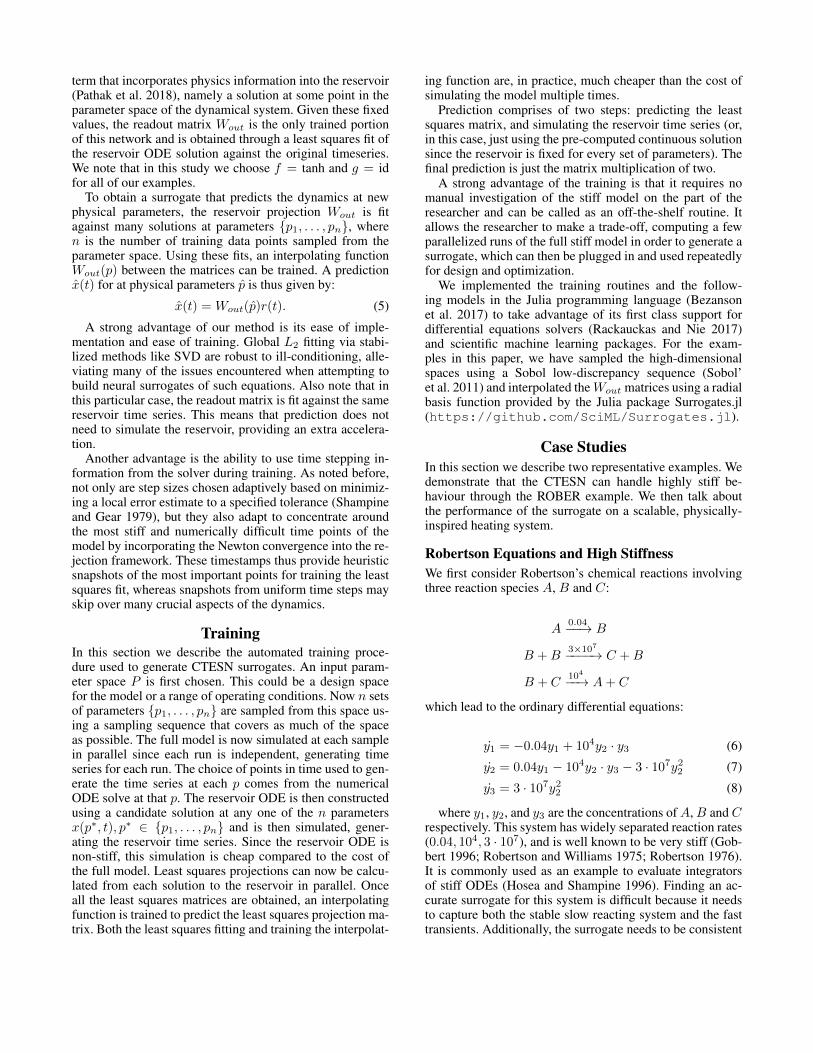
term that incorporates physics information into the reservoir(Pathak et al. 2018), namely a solution at some point in theparameter space of the dynamical system. Given these fixedvalues, the readout matrix Wout is the only trained portionof this network and is obtained through a least squares fit ofthe reservoir ODE solution against the original timeseries.We note that in this study we choose f = tanh and g = idfor all of our examples.

To obtain a surrogate that predicts the dynamics at newphysical parameters, the reservoir projection Wout is fitagainst many solutions at parameters {p1, . . . , pn}, wheren is the number of training data points sampled from theparameter space. Using these fits, an interpolating functionWout(p) between the matrices can be trained. A predictionx(t) for at physical parameters p is thus given by:

x(t) = Wout(p)r(t). (5)

A strong advantage of our method is its ease of imple-mentation and ease of training. Global L2 fitting via stabi-lized methods like SVD are robust to ill-conditioning, alle-viating many of the issues encountered when attempting tobuild neural surrogates of such equations. Also note that inthis particular case, the readout matrix is fit against the samereservoir time series. This means that prediction does notneed to simulate the reservoir, providing an extra accelera-tion.

Another advantage is the ability to use time stepping in-formation from the solver during training. As noted before,not only are step sizes chosen adaptively based on minimiz-ing a local error estimate to a specified tolerance (Shampineand Gear 1979), but they also adapt to concentrate aroundthe most stiff and numerically difficult time points of themodel by incorporating the Newton convergence into the re-jection framework. These timestamps thus provide heuristicsnapshots of the most important points for training the leastsquares fit, whereas snapshots from uniform time steps mayskip over many crucial aspects of the dynamics.

TrainingIn this section we describe the automated training proce-dure used to generate CTESN surrogates. An input param-eter space P is first chosen. This could be a design spacefor the model or a range of operating conditions. Now n setsof parameters {p1, . . . , pn} are sampled from this space us-ing a sampling sequence that covers as much of the spaceas possible. The full model is now simulated at each samplein parallel since each run is independent, generating timeseries for each run. The choice of points in time used to gen-erate the time series at each p comes from the numericalODE solve at that p. The reservoir ODE is then constructedusing a candidate solution at any one of the n parametersx(p∗, t), p∗ ∈ {p1, . . . , pn} and is then simulated, gener-ating the reservoir time series. Since the reservoir ODE isnon-stiff, this simulation is cheap compared to the cost ofthe full model. Least squares projections can now be calcu-lated from each solution to the reservoir in parallel. Onceall the least squares matrices are obtained, an interpolatingfunction is trained to predict the least squares projection ma-trix. Both the least squares fitting and training the interpolat-

ing function are, in practice, much cheaper than the cost ofsimulating the model multiple times.

Prediction comprises of two steps: predicting the leastsquares matrix, and simulating the reservoir time series (or,in this case, just using the pre-computed continuous solutionsince the reservoir is fixed for every set of parameters). Thefinal prediction is just the matrix multiplication of two.

A strong advantage of the training is that it requires nomanual investigation of the stiff model on the part of theresearcher and can be called as an off-the-shelf routine. Itallows the researcher to make a trade-off, computing a fewparallelized runs of the full stiff model in order to generate asurrogate, which can then be plugged in and used repeatedlyfor design and optimization.

We implemented the training routines and the follow-ing models in the Julia programming language (Bezansonet al. 2017) to take advantage of its first class support fordifferential equations solvers (Rackauckas and Nie 2017)and scientific machine learning packages. For the exam-ples in this paper, we have sampled the high-dimensionalspaces using a Sobol low-discrepancy sequence (Sobol’et al. 2011) and interpolated the Wout matrices using a radialbasis function provided by the Julia package Surrogates.jl(https://github.com/SciML/Surrogates.jl).

Case StudiesIn this section we describe two representative examples. Wedemonstrate that the CTESN can handle highly stiff be-haviour through the ROBER example. We then talk aboutthe performance of the surrogate on a scalable, physically-inspired heating system.

Robertson Equations and High StiffnessWe first consider Robertson’s chemical reactions involvingthree reaction species A, B and C:

A0.04−−→ B

B +B3×107−−−−→ C +B

B + C104−−→ A+ C

which lead to the ordinary differential equations:

y1 = −0.04y1 + 104y2 · y3 (6)

y2 = 0.04y1 − 104y2 · y3 − 3 · 107y22 (7)

y3 = 3 · 107y22 (8)

where y1, y2, and y3 are the concentrations of A, B and Crespectively. This system has widely separated reaction rates(0.04, 104, 3 · 107), and is well known to be very stiff (Gob-bert 1996; Robertson and Williams 1975; Robertson 1976).It is commonly used as an example to evaluate integratorsof stiff ODEs (Hosea and Shampine 1996). Finding an ac-curate surrogate for this system is difficult because it needsto capture both the stable slow reacting system and the fasttransients. Additionally, the surrogate needs to be consistent

with this system’s implicit physical constraints, such as theconservation of matter (y1 + y2 + y3 = 1) and positivity ofthe variables (yi > 0), in order to provide a stable solution.

A surrogate was trained by sampling 1000 sets of param-eters from the Cartesian parameter space [0.036, 0.044] ×[2.7 × 107, 3.3 × 107] × [9 × 103, 1.1 × 104] using Sobolsampling so as to evenly cover the whole space. We trainon the time series of the three states themselves as outputs.A least squares projection Wout was fit for each set of pa-rameters, and then a radial basis function was used to inter-polate between the matrices. The prediction workflow is asfollows: given a set of parameters whose time series is de-sired, the radial basis function predicts the projection matrix.The pre-simulated reservoir is then sampled at the desiredtime points, and a matrix multiplication with the predictedWout gives us the desired prediction. Figure 1 shows a com-parison between the CTESN, ESN, PINN and LSTM meth-ods. The PINN data is reproduced from (Ji et al. 2020) andthe ESN was trained using 101 time points uniformly sam-pled from the time span, while CTESN used 61 adaptivelysampled time points informed by the ODE solver (Rosen-brock23 (Shampine 1982)).

The CTESN method is able to accurately capture boththe slow and fast transients and respect the conservationof mass. The ESN is able to accurately predict at the timepoints it was trained on, but many features are missed. Theuniform stepping completely misses the fast transient riseat t = 10−4 because the uniform intervals do not samplepoints from that time scale. Additionally, the first sampledtime point at t = 100 is far into the concentration drop ofy1 which leads to an inaccurate prediction before the systemsettles into near steady state behavior. As stated earlier, theCTESN uses information from a stiff ODE solver to choosethe right points along the time span to accurately capturemulti-scale behaviour with less training data than the ESN.In order to compare the discrete ESN to the continuous re-sult, a cubic spline was fit to its 101 evenly spaced predictionpoints.

The PINN was trained by sampling 2500 logarithmicallyspaced points across the time span. The network used wasa 3-layer multi-layer perceptron with 128 nodes per hiddenlayer and the Gaussian Error Linear Unit activation func-tion (Hendrycks and Gimpel 2016). The layers were ini-tialed using Xavier initialization (Glorot and Bengio 2010),and trained with the ADAM optimizer (Kingma and Ba2019) at a learning rate of 10−3 for 300,000 epochs withmini batch size of 128. Figure 2 shows the convergence plotas the PINN trains on the ROBER equations. The LSTMnetwork used a similar architecture to the PINN, but withLSTM hidden layers instead of fully connected layers. Itused 2500 logarithmically spaced points and was trained for2000 epochs until convergence.

Figure 1 highlights how the trained PINN fails to cap-ture both the fast and the slow transients and do not re-spect mass conservation. Our collaborators investigated whyPINNs fail to solve these equations in (Ji et al. 2020). Thereason for the difficulty can be attributed to recently iden-tified results in gradient pathologies in the training arisingfrom stiffness (Wang, Teng, and Perdikaris 2020). With a

0 1×105 2×105 3×105

Number of epochs

1000

1500

2000

2500

3000

Loss

PINN training on the Robertson's Equations

Figure 2: Training a PINN on the Robertson’s Equations:PINN was trained for 300,000 epochs using the ADAM op-timizer with a learning rate of 10−3, by which time the lossseems to saturate. The hyperparameters of the PINN can befound in the Case Studies section.

highly ill-conditioned Hessian in the training process dueto the stiffness of the equation, it is very unlikely for localoptimization to find a parameters which make an accurateprediction. We additionally note stiff systems of this formmay be hard to capture by neural networks directly as neu-ral networks show a bias towards low frequency functions(Rahaman et al. 2019).

Stiffly-Aware Surrogates of HVAC SystemsOur second test problem is a scalable benchmark used inthe engineering community (Casella 2015). It is a simpli-fied, lumped-parameter model of a heating system with acentral heater supplying heat to several rooms through a dis-tribution network. Each room has an on-off controller withhysteresis which provides very fast localized action (Ranadeand Casella 2014). The resulting system of equations is thusvery stiff and unable to be solved by standard explicit timestepping methods.

The size of the heating system is scaled by a parameterN which refers to the number of users/rooms. Each roomis governed by two equations corresponding to its temper-ature and the state of its on-off controller. The tempera-ture of fluid supplying heat to each room is governed byone equation. This produces a system with 2N + 1 cou-pled non-linear equations. This “scalability” lets us test howour CTESN surrogate scales. To train the surrogate, we de-fine a parameter space P under which we expect it to op-erate. First, we assume set point temperature of each roomto be between 17◦C and 23◦C. Each room is warmed bya heat conducting fluid, whose set point is between 65◦Cand 75◦C. Thus the parameter space over which we expectour surrogate to work is the rectangular space denoted by[17◦C, 23◦C]× [65◦C, 75◦C].

We used a reservoir size of 3000 and sampled 100 setsof parameters from this space using Sobol sampling, and fitleast squares projection matrices Wout between each solu-tion and the reservoir. For a system with N rooms, we train

Figure 3: Validating the surrogate of the scalable heat-ing system with 10 rooms. When tested with parametersit has not seen in training, our surrogate is able to repro-duce the behaviour of the system to within 0.01% error.The surrogate is trained on 100 points sampled from the[17◦C, 23◦C]× [65◦C, 75◦C] where the ranges represent setpoint temperature of each room and set point of the fluidsupplying heat to the rooms respectively. The test parame-ters that validated here are [21◦C, 71◦C]. More details ontraining can be found in the Case Studies section.

Figure 4: Reliability of surrogate through parameterspace. We sampled our grid at over 500 grid points and plot-ted a heatmap of test error through our parameter space. Wefind our surrogate performs reliably even at the border of ourspace with error within 0.1%

40010 100

Figure 5: Scaling performance of surrogate on heatingsystem. We compare the time taken to simulate the full stiffmodel to the trained surrogate with 10, 20, 30 , 40, 50, 60,70, 80, 90, 100, 200 and 400 rooms. We observe a speedupof up to 98x. The surrogate was trained by sampling 100 setsof parameters from our input space, with a reservoir size of3000.

on N + 1 outputs, namely the temperature of each room,and the temperature of the heat conducting fluid. Figure 3demonstrates that the training technique is accurately ableto find matrices Wout which capture the stiff system within0.01% error on a test parameters. We then fit an interpo-lating radial basis function Wout(p). Figure 4 demonstratesthat the interpolated Wout(p) is able to adequately capturethe dynamics throughout the trained parameter space. Lastly,Figure 5 demonstrates the O(N) cost of the surrogate eval-uation, which in comparison to the O(N3) cost of a generalimplicit ODE solver (due to the LU-factorizations) leads toan increasing gap in the solver performance as N increases.At the high end of our test, the surrogate accelerates a 801dimensional stiff ODE system by approximately 98x.

Conclusion & Future WorkWe present CTESNs, a data-driven method for generatingsurrogates of nonlinear ordinary differential equations withdynamics at widely separated timescales. Our method main-tains accuracy for different parameters in a chosen parame-ter space, and shows favourable scaling with system size ona physics-inspired scalable model. This method can be ap-plied to any ordinary differential equation without requiringthe scientist to simplify the model before surrogate applica-tion, greatly improving productivity.

In future work, we plan to extend the formulation to takein forcing functions.This entails that the reservoir needs tobe simulated every single time a prediction is made, addingto running time, but we do note that numerically simulatingthe reservoir is quite fast in practice as it is non-stiff, andthus techniques which regenerate reservoirs on demand willlikely not incur a major run time performance cost.

Our method utilizes the continuous nature of differentialequation solutions. Hybrid dynamical systems, such as thosewith event handling (Ellison 1981), can introduce discon-tinuities into the system which will require extensions to

our method. Further extensions to the method will handleboth derivative discontinuities and events present in Filip-pov dynamical systems (Filippov 2013).Further opportuni-ties could explore utilizing more structure within equationsfor building a more robust CTESN or decrease the necessarysize of the reservoir.

To train both the example problems in this paper, we re-quired no knowledge of the physics. This presents an oppor-tunity to train surrogates of black-box systems.

AcknowledgementThe information, data, or work presented herein was fundedin part by the Advanced Research Projects Agency-Energy(ARPA-E), U.S. Department of Energy, under Award Num-bers DE-AR0001222 and DE-AR0001211, and NSF awardsOAC-1835443 and IIP-1938400. The views and opinionsof authors expressed herein do not necessarily state or re-flect those of the United States Government or any agencythereof. The authors thank Francesco Martinuzzi for review-ing drafts of this paper.

ReferencesBenner, P.; Gugercin, S.; and Willcox, K. 2015. A surveyof projection-based model reduction methods for parametricdynamical systems. SIAM review 57(4): 483–531.

Bezanson, J.; Edelman, A.; Karpinski, S.; and Shah, V. B.2017. Julia: A fresh approach to numerical computing.SIAM review 59(1): 65–98.

Butcher, J. B.; Verstraeten, D.; Schrauwen, B.; Day, C. R.;and Haycock, P. W. 2013. Reservoir computing and extremelearning machines for non-linear time-series data analysis.Neural networks 38: 76–89.

Casella, F. 2015. Simulation of large-scale models in Mod-elica: State of the art and future perspectives. In Proceedingsof the 11th International Modelica Conference, 459–468.

Chattopadhyay, A.; Hassanzadeh, P.; and Subramanian, D.2020. Data-driven predictions of a multiscale Lorenz 96chaotic system using machine-learning methods: reservoircomputing, artificial neural network, and long short-termmemory network. Nonlinear Processes in Geophysics 27(3):373–389.

Chattopadhyay, A.; Hassanzadeh, P.; Subramanian, D.; andPalem, K. 2019. Data-driven prediction of a multi-scaleLorenz 96 chaotic system using a hierarchy of deep learn-ing methods: Reservoir computing, ANN, and RNN-LSTM.

Doan, N. A. K.; Polifke, W.; and Magri, L. 2019. Physics-informed echo state networks for chaotic systems forecast-ing. In International Conference on Computational Science,192–198. Springer.

Eilertsen, J.; and Schnell, S. 2020. The Quasi-State-StateApproximations revisited: Timescales, small parameters,singularities, and normal forms in enzyme kinetics. Mathe-matical Biosciences 108339.

Ellison, D. 1981. Efficient automatic integration of ordinarydifferential equations with discontinuities. Mathematics andComputers in Simulation 23(1): 12–20.Evanusa, M.; Aloimonos, Y.; and Fermuller, C. 2020.Deep Reservoir Computing with Learned Hidden ReservoirWeights using Direct Feedback Alignment. arXiv preprintarXiv:2010.06209 .Filippov, A. F. 2013. Differential equations with discontin-uous righthand sides: control systems, volume 18. SpringerScience & Business Media.Flach, E. H.; and Schnell, S. 2006. Use and abuse of thequasi-steady-state approximation. IEE Proceedings-SystemsBiology 153(4): 187–191.Frangos, M.; Marzouk, Y.; Willcox, K.; and van Bloe-men Waanders, B. 2010. Surrogate and reduced-order mod-eling: a comparison of approaches for large-scale statisticalinverse problems [Chapter 7] .Gear, C. W. 1971. Numerical initial value problems in ordi-nary differential equations. nivp .Glorot, X.; and Bengio, Y. 2010. Understanding the diffi-culty of training deep feedforward neural networks. In Pro-ceedings of the thirteenth international conference on artifi-cial intelligence and statistics, 249–256.Gobbert, M. K. 1996. Robertson’s example for stiff differ-ential equations. Arizona State University, Technical report.Grezes, F. 2014. Reservoir Computing. Ph.D. thesis, PhDthesis, The City University of New York.Hadjinicolaou, M.; and Goussis, D. A. 1998. Asymptoticsolution of stiff PDEs with the CSP method: the reactiondiffusion equation. SIAM Journal on Scientific Computing20(3): 781–810.Hairer, E.; and Wanner, G. 1999. Stiff differential equationssolved by Radau methods. Journal of Computational andApplied Mathematics 111(1-2): 93–111.Hendrycks, D.; and Gimpel, K. 2016. Gaussian error linearunits (gelus). arXiv preprint arXiv:1606.08415 .Henry, A.; and Martin, O. C. 2016. Short relaxation timesbut long transient times in both simple and complex reactionnetworks. Journal of the Royal Society Interface 13(120):20160388.Hindmarsh, A.; and Petzold, L. 2005. LSODA, OrdinaryDifferential Equation Solver for Stiff or Non-stiff System .Hindmarsh, A. C.; Brown, P. N.; Grant, K. E.; Lee, S. L.;Serban, R.; Shumaker, D. E.; and Woodward, C. S. 2005.SUNDIALS: Suite of nonlinear and differential/algebraicequation solvers. ACM Transactions on Mathematical Soft-ware (TOMS) 31(3): 363–396.Hosea, M.; and Shampine, L. 1996. Analysis and imple-mentation of TR-BDF2. Applied Numerical Mathematics20(1-2): 21–37.Jaeger, H. 2003. Adaptive nonlinear system identificationwith echo state networks. In Advances in neural informationprocessing systems, 609–616.

Jaeger, H.; Lukosevicius, M.; Popovici, D.; and Siewert, U.2007. Optimization and applications of echo state networkswith leaky-integrator neurons. Neural networks 20(3): 335–352.

Ji, W.; Qiu, W.; Shi, Z.; Pan, S.; and Deng, S. 2020. Stiff-PINN: Physics-Informed Neural Network for Stiff ChemicalKinetics. arXiv preprint arXiv:2011.04520 .

Kim, Y.; Choi, Y.; Widemann, D.; and Zohdi, T. 2020. A fastand accurate physics-informed neural network reduced or-der model with shallow masked autoencoder. arXiv preprintarXiv:2009.11990 .

Kingma, D. P.; and Ba, J. A. 2019. A method for stochasticoptimization. arXiv 2014. arXiv preprint arXiv:1412.6980434.

Kramer, B.; and Willcox, K. E. 2019. Nonlinear model orderreduction via lifting transformations and proper orthogonaldecomposition. AIAA Journal 57(6): 2297–2307.

Kudithipudi, D.; Saleh, Q.; Merkel, C.; Thesing, J.; andWysocki, B. 2016. Design and analysis of a neuromemris-tive reservoir computing architecture for biosignal process-ing. Frontiers in neuroscience 9: 502.

Lukosevicius, M.; and Jaeger, H. 2009. Reservoir computingapproaches to recurrent neural network training. ComputerScience Review 3(3): 127–149.

Mattheakis, M.; and Protopapas, P. 2019. Recurrent Neu-ral Networks: Exploding, Vanishing Gradients & ReservoirComputing .

Nguyen, V.; Buffoni, M.; Willcox, K.; and Khoo, B. 2014.Model reduction for reacting flow applications. Interna-tional Journal of Computational Fluid Dynamics 28(3-4):91–105.

Ozturk, M. C.; Xu, D.; and Prıncipe, J. C. 2007. Analy-sis and design of echo state networks. Neural computation19(1): 111–138.

Pathak, J.; Wikner, A.; Fussell, R.; Chandra, S.; Hunt, B. R.;Girvan, M.; and Ott, E. 2018. Hybrid forecasting of chaoticprocesses: Using machine learning in conjunction with aknowledge-based model. Chaos: An Interdisciplinary Jour-nal of Nonlinear Science 28(4): 041101.

Polydoros, A.; Nalpantidis, L.; and Kruger, V. 2015. Ad-vantages and limitations of reservoir computing on modellearning for robot control. In IROS Workshop on MachineLearning in Planning and Control of Robot Motion, Ham-burg, Germany.

Qian, E.; Kramer, B.; Peherstorfer, B.; and Willcox, K. 2020.Lift & Learn: Physics-informed machine learning for large-scale nonlinear dynamical systems. Physica D: NonlinearPhenomena 406: 132401.

Rackauckas, C.; and Nie, Q. 2017. Differentialequations. jl–a performant and feature-rich ecosystem for solving differ-ential equations in julia. Journal of Open Research Software5(1).

Rahaman, N.; Baratin, A.; Arpit, D.; Draxler, F.; Lin, M.;Hamprecht, F.; Bengio, Y.; and Courville, A. 2019. On the

spectral bias of neural networks. In International Confer-ence on Machine Learning, 5301–5310. PMLR.Raissi, M.; Perdikaris, P.; and Karniadakis, G. E. 2019.Physics-informed neural networks: A deep learning frame-work for solving forward and inverse problems involvingnonlinear partial differential equations. Journal of Compu-tational Physics 378: 686–707.Ranade, A.; and Casella, F. 2014. Multi-rate integrationalgorithms: a path towards efficient simulation of object-oriented models of very large systems. In Proceedings ofthe 6th International Workshop on Equation-Based Object-Oriented Modeling Languages and Tools, 79–82.Ratnaswamy, V.; Safta, C.; Sargsyan, K.; and Ricciuto,D. M. 2019. Physics-informed Recurrent Neural NetworkSurrogates for E3SM Land Model. AGUFM 2019: GC43D–1365.Robertson, H. 1976. Numerical integration of systems ofstiff ordinary differential equations with special structure.IMA Journal of Applied Mathematics 18(2): 249–263.Robertson, H.; and Williams, J. 1975. Some properties ofalgorithms for stiff differential equations. IMA Journal ofApplied Mathematics 16(1): 23–34.Schuster, S.; and Schuster, R. 1989. A generalizationof Wegscheider’s condition. Implications for properties ofsteady states and for quasi-steady-state approximation. Jour-nal of Mathematical Chemistry 3(1): 25–42.Shampine, L. F. 1982. Implementation of Rosenbrock meth-ods. ACM Transactions on Mathematical Software (TOMS)8(2): 93–113.Shampine, L. F.; and Gear, C. W. 1979. A user’s view ofsolving stiff ordinary differential equations. SIAM review21(1): 1–17.Sobol’, I. M.; Asotsky, D.; Kreinin, A.; and Kucherenko,S. 2011. Construction and comparison of high-dimensionalSobol’generators. Wilmott 2011(56): 64–79.Soderlind, G.; Jay, L.; and Calvo, M. 2015. Stiffness 1952–2012: Sixty years in search of a definition. BIT NumericalMathematics 55(2): 531–558.Thomas, P.; Straube, A. V.; and Grima, R. 2011. Commu-nication: limitations of the stochastic quasi-steady-state ap-proximation in open biochemical reaction networks.Turanyi, T.; Tomlin, A.; and Pilling, M. 1993. On the er-ror of the quasi-steady-state approximation. The Journal ofPhysical Chemistry 97(1): 163–172.van de Plassche, K.; Citrin, J.; Bourdelle, C.; Camenen, Y.;Casson, F.; Felici, F.; Horn, P.; Ho, A.; Van Mulders, S.;Koechl, F.; et al. 2020. Fast surrogate modelling of turbu-lent transport in fusion plasmas with physics-informed neu-ral networks .Verwer, J. G. 1994. Gauss–Seidel iteration for stiff ODEsfrom chemical kinetics. SIAM Journal on Scientific Com-puting 15(5): 1243–1250.Vlachas, P. R.; Pathak, J.; Hunt, B. R.; Sapsis, T. P.; Girvan,M.; Ott, E.; and Koumoutsakos, P. 2020. Backpropagation

algorithms and reservoir computing in recurrent neural net-works for the forecasting of complex spatiotemporal dynam-ics. Neural Networks .Wang, S.; Teng, Y.; and Perdikaris, P. 2020. Understand-ing and mitigating gradient pathologies in physics-informedneural networks. arXiv preprint arXiv:2001.04536 .Wanner, G.; and Hairer, E. 1996. Solving ordinary differen-tial equations II. Springer Berlin Heidelberg.Willard, J.; Jia, X.; Xu, S.; Steinbach, M.; and Kumar, V.2020. Integrating physics-based modeling with machinelearning: A survey. arXiv preprint arXiv:2003.04919 .Zhang, R.; Zen, R.; Xing, J.; Arsa, D. M. S.; Saha, A.; andBressan, S. 2020. Hydrological Process Surrogate Mod-elling and Simulation with Neural Networks. In Pacific-Asia Conference on Knowledge Discovery and Data Mining,449–461. Springer.