Accelerating seismicity before the 2017 Nuugaatsiaq1

landslide revealed with unsupervised deep learning2

L. Seydoux1, R. Balestriero2, P. Poli1, M. de Hoop3, M. Campillo1,3

and R. Baraniuk24

1Institut des sciences de la Terre, Universite Grenoble-Alpes, UMR CNRS 5375, France5

2Electrical & Computational Engineering, Rice University, Houston, TX, 77005, USA6

3Computational & Applied Mathematics, Rice University, Houston, TX, 77005, USA7

May 19, 20208

Abstract9

The continuously growing amount of seismic data collected worldwide10

is outpacing our abilities for analysis, since to date, such datasets have11

been analyzed in a human-expert-intensive, supervised fashion. Moreover,12

analyses that are conducted can be strongly biased by the standard models13

employed by seismologists. In response to both of these challenges, we14

develop a new unsupervised machine learning framework for detecting and15

clustering seismic signals in continuous seismic records. Our approach16

combines a deep scattering network and a Gaussian mixture model to17

cluster seismic signal segments and detect novel structures. To illustrate18

the power of the framework, we analyze seismic data acquired during19

the June 2017 Nuugaatsiaq, Greenland landslide. We demonstrate the20

blind detection and recovery of the repeating precursory seismicity that21

was recorded before the main landslide rupture, which suggests that our22

approach could lead to more informative forecasting of the seismic activity23

in seismogenic areas.24

1

Introduction25

Current analysis tools for seismic data lack the capacity to investigate the mas-26

sive volumes of data collected worldwide in a timely fashion, likely leaving cru-27

cial information undiscovered. The current reliance on human-expert analysis28

of seismic records is not only unscalable, but it can also impart a strong bias29

that favors the observation of already known signals [1]. As a case in point,30

consider the detection and characterization of non-volcanic tremors, which were31

first observed in the southwestern Japan subduction zone two decades ago [2].32

The complex signals generated by such tremors are very hard to detect in some33

regions due to their weak amplitude. Robustly detecting these new classes of34

seismic signals in a model-free fashion would have a major impact in seismology35

(e.g., for the purpose of forecasting earthquakes), since we would better under-36

stand the physical processes of seismogenic zones (subduction, faults, etc.).37

Recently, techniques from machine learning have opened up new avenues for38

rapidly exploring large seismic datasets with minimum a priori knowledge. Ma-39

chine learning algorithms are data-driven tools that approximate non-linear re-40

lationships between observations and labels (supervised learning) or that reveal41

patterns from unlabeled data (unsupervised learning). Supervised algorithms42

rely on the quality of the predefined labels, often obtained via classical algo-43

rithms [3, 4] or even manually [5, 6, 7, 8]. Inherently, supervised strategies are44

used to learn how to detect or classify specific classes of already-known signals45

and, therefore, cannot be used for discovering new classes of seismic signals.46

Seismology can significantly benefit from the development of unsupervised ap-47

proaches because the data is mostly unlabeled. Unsupervised tools are likely the48

best candidates to explore seismic data without the need for any explicit signal49

model and hence, discover new classes of seismic signals. For this reason, un-50

supervised methods are more relevant for seismology, where the data is largely51

unlabeled and new classes of seismic signals should be sought. While supervised52

strategies are often easier to implement thanks to the evaluation of a prediction53

error, unsupervised strategies mostly rely on implicit models that are challeng-54

2

ing to design. Unsupervised-learning based studies have mostly been applied to55

data from volcano monitoring systems, where a large variety of seismo-volcanic56

signals is usually observed [9, 10, 11, 12]. Some unsupervised methods have also57

been recently applied to induced seismicity [13, 14], global seismicity [15], and58

local-vs-distance earthquakes [16]. In both cases (supervised or unsupervised),59

the keystone to success lies in the data representation namely, we need to define60

an appropriate set of relevant waveform features for solving the task of interest.61

The features can be manually defined [17, 7, 18] or learned with appropriates62

techniques such as artificial neural networks [5, 3], the latter belonging to the63

field of deep learning.64

In this paper, we develop a new unsupervised deep-learning method for clus-65

tering signals in continuous multichannel seismic time-series. Our strategy com-66

bines a deep scattering network [19, 20] for automatic feature extraction and67

a Gaussian mixture model for clustering. Deep scattering networks belong to68

the family of deep convolutional neural networks, where the convolutional filters69

are restricted to wavelets and with modulus activations [19]. The restriction to70

wavelets filters allows the deep scattering networks to have explicit and physics-71

related properties that greatly simplifies the architecture design in contrast with72

classical deep convolutional neural network (frequency band, time scales of in-73

terest, amplitudes). Scattering networks have shown to perform high-quality74

classification of audio signals [21, 20, 22] and electrocardiograms [23]. A deep75

scattering network decomposes the signal’s structure through a tree of wavelet76

convolutions, modulus operations and average-pooling, providing a stable rep-77

resentation at multiple time and frequency scales [20]. The resulting represen-78

tation is particularly suitable for discriminating complex seismic signals that79

may differ in nature (source and propagation effects) with several order of dif-80

ferent durations, amplitudes and frequency contents. After decomposing the81

time series with the deep scattering network, we exploit the representation in82

a two-dimensional feature space that results from a dimension reduction for vi-83

sualization and hence, interpretation purposes. The two-dimensional features84

are finally fed to a Gaussian mixture model for clustering the different time85

3

segments.86

The design of the wavelet filters have been conducted in many studies, and in87

each case led to data-adapted filter banks based on intuition on the underlying88

physics [24, 25, 26] (e.g. music classification, speech processing, bioacoustics,89

etc.). In order to follow the same idea of optimal wavelet design in a fully ex-90

plorative way, we propose to learn the mother wavelet of each filter bank with91

respect to the clustering loss. By imposing a reconstruction constraint to the92

different layers of the deep scattering network, we guarantee to fully fit the93

data distribution together with improving the clustering quality. Our approach94

therefore preserves the structure of a deep scattering network while learning95

a representation relevant for clustering. It is an unsupervised representation96

learning method located in between the time-frequency analysis widely used in97

seismology and the deep convolutional neural networks. While classical convo-98

lutional networks usually require a large amount of data for learning numerous99

coefficients, our strategy can still work with small datasets thanks to the re-100

striction to wavelet filters. In addition, the architecture of the deep scattering101

network is dictated by physical intuitions (frequency and time scales of interest).102

This is in contrast to the tedious task of designing deep convolutional neural103

networks, which today is typically pursued empirically.104

Results105

Seismic records of the 2017 Nuugaatsiaq landslide. We apply our strat-106

egy for blindly clustering and detecting the low-amplitude precursory seismic-107

ity [27] to the June 2017 landslide that occurred near Nuugaatsiaq, Greenland108

at 23:39 UTC. The volume of the rockfall was estimated between 35 to 51 mil-109

lion cubic meters by differential digital elevation models, forming thus a massive110

landslide [28]. This landslide triggered tsunami waves that impacted the small111

town of Nuugaatsiaq and caused four reported injuries [28].112

The continuous seismic wavefield was recorded by a three-component broad-113

band seismic station (NUUG) located 30 km away from the landslide epicenter114

4

(Fig. 1A). We select the daylong three-component seismograms from 2017-06-17115

00:00 to 2017-06-17 23:38 in order to remove the signal due to the mainshock116

and focus on the content of the seismic wavefield recorded before. A detailed117

inspection of the east component records revealed that a small event was occur-118

ring repetitively before the landslide, starting approximately 9 hours before the119

rupture and accelerating over time [27, 29]. The accelerating behavior of this120

seismicity suggests that an unstable initiation was at work before the massive121

landslide. This signal is not directly visible in raw seismic records; it is of very122

weak amplitude, has a smooth envelope, and most of its energy located in be-123

tween 2 and 8 Hz (see a zoom onto the last 4 hours of data in Fig. 1B) and was124

first highlighted with three-component template matching [27]. While some of125

these events may be visible in the seismograms filtered between 2 and 9 Hz at126

times close to the landslide, a large part are hidden in the background noise [27].127

The structure of such signal makes it hard to detect via traditional detection128

algorithms such as STA/LTA (the ratio between Short-Term Average and the129

Long-Term Average of the seismic signal [30]), because they are sensitive to130

brutal signal changes with decent signal-to-noise ratios [15]. Besides, STA/LTA131

only delivers an information about the presence of a signal in the continious132

trace without any clue of the similarity with other signals, which is our primary133

goal here.134

The template matching strategy consists in a search for similar events in a135

time series with evaluating a similarity function (cross-correlation) between a136

pre-defined example of the event (template) and the continuous records. This137

method is sensitive to the analyzed frequency band, the duration and the qual-138

ity of the template (often manually defined), making the template matching139

strategy a severely supervised strategy, yet powerful [31]. Revealing this kind140

of seismicity with an unsupervised template-matching based strategy could be141

done with performing the cross-correlation of all time segments (autocorrela-142

tion), testing every time segments as potential template event [32]. Considering143

that several durations, frequency bands, etc. should be tested, this approach144

is nearly impossible to perform onto large datasets for computational limita-145

5

tions [15].146

In the present study, we propose to highlight this precursory event in a147

blind way over a daylong, raw seismic record. Our goal is to show that even148

if the precursory signal was not visible after a detailed manual inspection of149

the seismograms and late times, it could have been correctly detected by our150

approach. The reader should bear in mind that clustering is an exploratory151

task [33]; we do not aim at overperforming techniques like template matching,152

but to provide a first, preliminary and statistical result that could simplify153

further detailed analyses like template selection for template matching detection.154

Feature extraction from a learnable deep scattering network. A dia-155

gram of the proposed clustering algorithm is shown in Fig 2. The theoretical156

definitions are presented in the supplementary materials. Our model first builds157

a deep scattering network that consists in a tree of wavelet convolutions and158

modulus operations (Eq. S5). At each layer, we define a bank of wavelet filters159

with constant quality factor from dilations and stretching of a mother wavelet.160

This is done according to a geometric progression in the time domain in order161

to cover a frequency range of interest (the scale defined in Eq. S2). The input162

seismic signal is initially convolved with a first bank of wavelets at different163

scales, which modulus leads to a first-order scalogram (conv1), a time and fre-164

quency representation of one-dimensional signals widely used in seismology [34].165

In order to speed up computations, we low-pass filter the coefficients in conv1,166

and perform a temporal downsampling (pool1) with an average-pooling oper-167

ation [35]. The coefficients of pool1 are then convolved with a second wavelet168

bank, forming the second-order convolution layer (conv2). These succession of169

operations can be seen as a two-layer demodulation, where the input signal’s170

envelope is extracted at the first layer (conv1) for several carrier frequencies,171

and where the frequency content of each envelope is decomposed again at the172

second layer (conv2) [20].173

We define a deep scattering network as the sequence of convolution-modulus174

operations performed at higher orders, allowing to scatter the signal structure175

6

through the tree of time and frequency analyses. We finally obtain a locally176

invariant signal representation by applying an average-pooling operation to the177

all-order pooling layers [19, 21, 20]. This pooling operation is adapted for con-178

catenation, with an equal number of time samples at each layer (Fig. 2). The179

scattering coefficients are invariant to local time translation, small signal de-180

formations and signal overlapping. They incorporate multiple time scales (at181

different layers) and frequencies scales (different wavelets). The tree of op-182

erations performed in a scattering network forms a deep convolutional neural183

networks, where the convolutional filters are restricted to wavelets, and where184

the activation function is the modulus operator [19]. Scattering networks are185

located in between (1) classical time and frequency analysis routinely applied186

in seismology that is often limited to a typical time scale, and (2) deep con-187

volutional neural networks where the unconstrained filters are often hard to188

interpret, and where the network architecture is often challenging to define. In189

contrast, deep scattering networks can be designed in a straightforward way,190

thanks to the analytic framework defined in [19].191

From one layer to another, we increase the frequency range of the filter banks192

in order to consider at the same time small-duration details of the waveform,193

and larger-duration histories (see Table 1, case D for the selected architecture in194

the present study). The number of wavelets per octaves and number of octaves195

defines the frequency resolution and bandwidth of each layer, and the depth196

(total number of layers) of the scattering network controls the final temporal197

resolution of the analysis. Following the recommendations cross-validated onto198

audio signal classification [20], we use a large number of filters at the first layer,199

and we gradually increase the number of octaves while reducing the number of200

wavelets per octave from the first to the last layer (Table 1, case D). That way,201

the representation is highly redundant at the layer conv1 and gets sparser at202

the higher-order layers conv2 and conv3, where fewer filters are used at each203

frequency to decompose the signal. This has the main effect of improving the204

contrast between signals of different nature [20]. We finally choose the network205

depth based on the range of time scales of interest. In the present study, we aim206

7

at investigating mostly impulsive earthquake-like signals that may last between207

several seconds to less that one minute. A deeper scattering network could be208

of interest in order to analyze the properties of longer-duration signals such209

as seismic tremors [36] or background seismic noise. Finally, with our choice of210

pooling factors, we obtain a temporal resolution of 35 seconds for each scattering211

coefficient.212

Clustering seismic signals. The scattering coefficients are built in order213

to be linearly separable [23] so that the need for a high-dimensional scatter-214

ing representation is greatly reduced. In fact, it is even possible to enforce215

the learning to favor wavelets that not only solve the task but also provide a216

lower-dimensional representation of the signal. We do so by reducing the di-217

mension of the scattering coefficients with projection onto the first two principal218

components (Eq. S10). This also improves the data representation in two di-219

mensions and eases the interpretation. More flexibility could be also added to220

the procedure by using the latent representation of an autoencoder instead of221

principal component analysis, because autoencoders can lower the dimension of222

any datasets with non-linear projections. However, such dimension reduction223

must be thoroughly investigated because it adds a higher-level complexity to224

the overall procedure (autoencoder learning rate, architecture, etc.), and will225

define the goal of future studies.226

The two-dimensional scattering coefficients are used to cluster the seismic227

data. We use a Gaussian mixture model [37] for clustering, where the idea is228

to find the set of K normal distributions of mean µk and covariance Σk (where229

k = 1 . . .K) that best describe the overall data (illustrated in Fig. 2 inset,230

and described in Eq. S11). A categorical variable is also inferred in order to231

allocate each data sample into each cluster in this procedure, which is the final232

result of our algorithm. Gaussian mixture model clustering can be seen as a233

probabilistic and more flexible version of the K-means clustering algorithm,234

where each covariance can be anisotropic, the clusters can be unbalanced in235

term of internal variance, and where the decision boundary is soft [37].236

8

Initialized with Gabor wavelets [38], we learn the parameters governing the237

shape of the wavelets with respect to the clustering loss (Eq. S8) with the238

Adam stochastic gradient descent [39] detailed in the supplementary material239

(Eq. S14). The clustering loss is defined as the negative log-likelihood of the240

data to be fully described by the set of normal distributions. We define the241

wavelets onto specific knots, and interpolate them with Hermite cubic splines242

onto the same time basis of the seismic data for applying the convolution (see243

the dedicated section in the material and methods). We ensure that the mother244

wavelet at each layer satisfies the mathematical definition of a wavelet filter245

in order to keep all the powerful properties of a deep scattering network [23].246

We finally add a constraint on the network in order to prevent the learning247

procedure to dropout some signals that make the clustering task hard (e.g.248

outlier signals). This is done by imposing a reconstruction loss from one layer249

to its parent signal, noticing that a signal should be reconstructed from the sum250

of the convolutions of itself with a bank of wavelet filters (Eq. S13).251

The number of clusters is also inferred by our procedure. We initialize the252

Gaussian mixture clustering algorithm with a (large) number K = 10 clusters253

at the first epoch, and let all of these components be used by the Expectation-254

Minimization strategy [37]. This is shown at the first epoch in the latent space255

in Fig. 3A, where the Gaussian component mean and covariance are shown in256

color with the corresponding population cardinality on the right-hand side. As257

the learning evolves, we expect the representation to change the coordinates258

of the two-dimensional scattering coefficients in the latent space (black dots),259

leading to Gaussian components that do not contribute anymore to fit the data260

distribution, and therefore to be automatically disregarded in the next iteration.261

We can therefore infer a number of clusters from a maximal value. At the first262

epoch (Fig. 3A), we observe that the seismic data samples are scattered in the263

latent space, and that the Gaussian mixture model used all of the 10 components264

to explain the data.265

The clustering loss decreases with the learning epochs (Fig. 3C). We declare266

the clustering to be optimal when the loss stagnates (reached after approxi-267

9

mately 7,000 epochs). The learning is done with batch-processing, a technique268

that allows for faster computation by randomly selecting smaller subsets of the269

full dataset. This also avoids falling into local minima, as we can observe around270

epoch 3,500, and guarantees to reaching a stable minimum that does not evolve271

anymore after epoch 7,000 (Fig. 3C). After 10,000 training epochs, as expected,272

we observe that the scattering coefficients have been concentrated around the273

clusters centroids obtained with the Gaussian mixture model (Fig. 3B). The set274

of useful components have been reduced to 4, a consequence of a better learned275

representation due to the learned wavelets at the last epoch (Fig. 3D). The276

cluster colors range from colder to warmer colors depending on the population277

size.278

The clustering loss improves by a factor of approximately 4.5 between the279

first and the last epoch (Fig. 3C). At the same time, we observe that the re-280

construction loss is more than 15 times smaller than at the first training epoch281

(Table 1). This indicates that the basis of wavelets filter banks used in the deep282

scattering network is powerful to accurately represent the seismic data with283

ensuring a good-quality clustering at the same time.284

Analysis of clusters. An analysis of the temporal evolution of the clusters285

is presented in Fig. 4. The within-cluster cumulative detections obtained af-286

ter training (epoch 10,000) are presented in Fig. 4A for clusters 1 and 2, and287

in Fig. 4B for clusters 2 and 3. The two most populated clusters 1 and 2288

(Fig. 4A) gather more than 90% of the overall data (observed on the histograms289

in Fig. 3B). They both show a linear detection rate over the day with no par-290

ticular concentration in time and, therefore, relate to the background seismic291

noise. Clusters 3 and 4 (Fig. 4B) show different non-linear trends that include292

10% of the remaining data.293

The temporal evolution of cluster 4 is presented in Fig. 4B. The time seg-294

ments that belong to cluster 4 are extracted and aligned to a reference time295

segment (at the top) with local cross-correlation for better readability (see fur-296

ther details about the strategy in the supplementary materials). We see that297

10

these time segments contain seismic events localized in time with relatively high298

signal-to-noise ratio and sharp envelope. These events do not show a strong299

similarity in time, but they strongly differ from the event belonging to other300

clusters, explaining why they have been gathered in the same cluster. The de-301

tection rate is sparse in time, indicating that cluster 4 is mostly related to a302

random background seismicity or other signals which interest is beyound the303

scope of the present manuscript.304

The temporal evolution of cluster 3 shows three behaviors. First, we observe305

a nearly-constant detection rate from the beginning of the day to approximately306

07:00. Second, the detection rate lowers between 07:00 and 13:00 where only 4%307

of the within-cluster detections are observed. An accelerating seismicity is finally308

observed from 13:00 up to the landslide time (23:39 UTC). The time segments309

belonging to cluster 3 are reported on Fig. 4D in gray colorscale, and aligned310

with local cross-correlation with a reference (top) time segment. The correlation311

coefficients obtained for the time lag that maximizes the alignment are indicated312

in orange color in Fig. 4E. As with the template matching strategy, we clearly313

observe the increasing correlation coefficient with the increasing event index [27],314

indicating that the signal-to-noise ratio increases towards the landslide rupture.315

This suggests that the repeating event may still exist earlier in the data even316

before 15:00, but that the detection threshold of the template matching method317

is limited by the signal-to-noise ratio [27]. In contrast, we observe that the318

probability of these 171 events remains high in our approach,with 97% of the319

precursory events previously found [27] recovered.320

A interesting observation is the change of behavior in the detection rate of321

this cluster at nearly 07:00 (Fig. 4B). The events that happened before 07:00322

have all a relatively high probability to belong to cluster 3, refuting the hy-323

pothesis that noise samples have randomly been misclassified by our strategy324

(Fig. 4E). The temporal similarity of all these events in Fig. 4D is particularly325

visible for later events (high index) because the signal-to-noise ratio of these326

events increases towards the landslide [27]. The two trends may be whether327

related to similar signals generated at same position (same propagation) with a328

11

different source, or by two types of alike-looking events that differ in nature, but329

that may have been gathered in the same cluster because they strongly differ330

from the other clusters. This last hypothesis can be tested with using hierarchi-331

cal clustering [40]. Our clustering procedure highlighted those 171 similar events332

in a totally unsupervised way, without the need of defining any template from333

the seismic data. The stack of the 171 waveforms is shown in black solid line in334

Fig. 4D, indicating that the template of these events is defined in a blind way335

thanks to our procedure. In addition, these events have very similar properties336

(duration, seismic phases, envelope) in comparison with the template defined337

in [27].338

Discussion and conclusions339

We have developed a new strategy for clustering and detecting seismic events in340

continuous seismic data. Our approach extends a deterministic deep scattering341

network by learning the wavelet filter-banks and applying a Gaussian mixture342

model. While scattering networks correspond to a special deep convolutional343

neural network with fixed wavelet filter-banks, we allow it to fit the data dis-344

tribution by learnability of the different mother wavelets; yet we preserve the345

structure of the deep scattering network allowing interpretability and theoretical346

guarantees. We combine the powerful representation of the learnable scattering347

network with Gaussian mixture clustering by learning the shape of the wavelet348

filters according to the clustering loss. This allows to learn a representation of349

multichannel seismic signals that maximizes the quality of clustering, leading350

to an unsupervised way of exploring possibly large datasets. We also impose a351

reconstruction loss as each layer of the deep scattering network, following the352

ideas of convolutional autoencoders, thus preventing to learn trivial solutions353

such as zero-valued filters.354

Our strategy is capable of blindly recovering the small-amplitude precur-355

sory signal reported in [27, 29]. This indicates that waveform templates can356

be recovered from our method without the need of any manual inspection of357

12

the seismic data prior to the clustering process, and tedious selection of wave-358

form template in order to perform high-quality detection. Such unsupervised359

strategy is of strong interest in the exploration of seismic datasets, where the360

structure of seismic signals can be complex (low-frequency earthquakes, non-361

volcanic tremors, distant vs. local earthquakes, etc.), and where some class of362

unknown signals is likely to be disregarded by a human expert.363

In the proposed workflow, only a few parameters need be chosen, namely364

the number of octaves and wavelets per octave at each layer J (`) and Q(`), the365

number of knots K the pooling factors and the network depth M . This choice366

of parameters is extremely constrained by the underlying physics. The number367

of octaves at each layer controls the lowest analyzed frequency at each layer,368

and therefore, the largest time scale. The pooling factor and number of layers369

M should be chosen according to the analyzed time scale at each layer, and370

the final maximal time scale of interest for the user. We discuss our choice of371

parameters with testing several parameter sets summarized in Table 1 and with372

corresponding results summarized in Fig. S5 for the cumulative detection curves,373

within-cluster population sizes and learned mother wavelets. All the results374

obtained with different parameters show extremely similar cluster shapes in the375

time domain, and the precursory signal accelerating shape is always recovered.376

We see that a low number of 3 or 4 clusters are found in almost all cases, with377

a highly similar detection rates over the day. Furthermore, we observe that the378

shape of the learned wavelets remain highly similar between the different data-379

driven tests, and in particular, the third-order wavelet is highly similar with all380

the tested parameters (Fig. 5G). This result makes sense because the coefficients381

that output from the last convolutional layer conv3 are over-represented in382

comparison with the other ones. We also observe that the procedure still works383

with only a few amount of data (Fig. 5A–C), a very strong advantage compared384

with classical deep convolutional neural networks that often require a large385

amount of data to be successfully applied.386

Besides being adapted to small amount of data, our strategy can also work387

with large amount of data, as scalability is garanteed by batch processing, and388

13

using only small-complexity operators (convolution and pooling). Indeed, batch389

processing allows to control the amount of data seen by the scattering network390

and GMM at a single iteration, each epoch being defined when the whole dataset391

have been analyzed by the algorithm. There is no limitation to the total amount392

of data being analyzed because only the selected segments at each iteration are393

fed to the network. At longer time scales, the number of clusters needed to fit394

the seismic data must change, however, with an expectation that the imbalance395

between clusters should increase. We illustrate this point another experiment396

performed on the continuous seismogram recorded at the same station over 17397

days, including the date of the landslide (from 2017-06-01 to 2017-06-18). With398

this larger amount of data, the clustering procedure still converges and exhibit399

9 new clusters. The hourly within-clusters detections of these new clusters400

are presented in Fig. 5. Among the different clusters found by our strategy,401

we observe that more than 93% of the data is identified in slowly evolving402

clusters, most likely related to fluctuations of the ambient seismic noise (Fig. 5,403

clusters A to E). The most populated clusters (A and B) occupy more than404

61% of the time, and are most likely related to diffuse wavefield without any405

particular dominating source. Interestingly, we observe two other clusters with406

large population with a strong localisation in time (clusters C and D in Fig. 5).407

A detailed analysis of the ocean-radiated microseismic energy [44, 45] allowed us408

to identify the location and dominating frequency of the sources reponsible for409

these clusters to be identified (illustrated in Fig. S2 and S3 in the supplementary410

material). The source time function of the best-matching microseismic sources411

have been reported on clusters C and D in Fig. 5.412

Compared with these long-duration clusters, the clustering procedure also413

reports very sparse clusters where less than 7% of the seismic data is present.414

Because of clustering instabilities caused by the large class imbalance of the seis-415

mic data, we decided to perform a second-order clustering on the low-populated416

clusters. This strategy follows the idea of hirearchical clustering [40], where417

the firstly identified clusters are analyzed several consecutive times in order to418

discover within-cluster families. For the sake of brevity, we do not intend to per-419

14

form a deep-hirarchical clustering in the present manuscript, but to illustrate420

the potential strength of such strategy in seismology, where the data is essen-421

tially class-imbalanced. We perform a new clustering from the data obtained in422

the merged low-populated clusters (F to I in Fig. 5). This additional clustering423

procedure detected two clusters presented in Fig. 6A. These two clusters have424

different temporal cumulated detections and exhibits different population sizes.425

A zoom of the cumulated within-cluster detections is presented in Fig. 6B, and426

show a high similarity with clusters 3 and 4 previously obtained in Fig. 3 from427

the daylong seismogram. This result clearly proves that the accelerating pre-428

cursor is captured by our strategy even when the data is highly imbalanced. If429

the scattering network provide highly relevant features, clustering seismic data430

with simple clustering algorithms can be a hard task that can be solved with hi-431

erachical clustering, as illustrated in the present study. This problem can also432

be better tackled by other clustering algorithms such as spectral clustering [41]433

which has the additional ability to detect outliers. Clustering the outlier signals434

may then be an alternative to GMM in that case. Another possibility would be435

to use the local similarity search with hashing functions [15] in order to improve436

our detection database onto large amount of seismic data.437

The structure of the scattering network shares some similarities with the438

FAST algorithm (for Fingerprint And Similarity Search [15]) from a architec-439

tural point of view. FAST uses a suite of deterministic operations in order to440

extract waveforms features and feed it to a hashing system in order to per-441

form a similarity search. The features are extracted from the calculation of442

spectrogram, Haar wavelet transforms and thresholding operations. While be-443

ing similar, the FAST algorithm involves a number of paramaters that are not444

connected to the underlying physics. For instance, the thresholding operation445

has to be manually inspected [15], as well as the size of the analyzing window.446

In comparison, our alrotihm’s parameters are based on physical intuition, and447

does not imply any signal windowing (only the resolution of the final result can448

be controlled). FAST is not a machine learning strategy because no learning449

is involved; in contrast, we do learn the representation of the seismic data that450

15

best solves the task of clustering. While FAST needs a large amount of data to451

be run in an optimal way [15], our algorithm still works with a few number of452

samples.453

This work shows that learning a representation of seismic data in order454

to cluster seismic events in continuous waveforms is a challenging task that455

can be tackled with deep learnable scattering networks. The blind detection456

of the seismic precursors to the 2017 Landslide of Nuugaatsiaq with a deep457

learnable scattering network is a strong evidence that weak seismic events of458

complex shape can be detected with a minimum amount of prior knowledge.459

Discovering new classes of seismic signals in continuous data can, therefore, be460

better addressed with such strategy, and could lead to a better forecasting of461

the seismic activity in seismogenic areas.462

Aknowldgements463

L.S., P.P. and M.C. acknowledge support from the European Research Council under464

the European Union Horizon 2020 research and innovation program (grant agree-465

ment no. 742335, F-IMAGE). M.V.d.H. gratefully acknowledges support from the466

Simons Foundation under the MATH + X program and from NSF under grant DMS-467

1815143. R.B. and R.G.B. were supported by NSF grants IIS-17-30574 and IIS-18-468

38177, AFOSR grant FA9550-18-1-0478, ONR grant N00014-18-12571, and a DOD469

Vannevar Bush Faculty Fellowship, ONR grant N00014-18-1-2047. L.S. thanks Ro-470

main Cosentino for very helpful discussions and comments. The facilities of IRIS471

Data Services, and specifically the IRIS Data Management Center, were used for472

access to waveforms and related metadata used in this study. IRIS Data Services473

are funded through the Seismological Facilities for the Advancement of Geoscience474

and EarthScope (SAGE) Project funded by the NSF under Cooperative Agreement475

EAR-1261681. The authors declare that they have no competing financial inter-476

ests. Correspondence and requests for materials should be addressed to L.S. (email:477

leonard.seydoux@univ-grenoble-alpes.fr).478

16

Figures and tables479

17

58°W 56°W 54°W 52°W 50°W70.5°N

71°N

71.5°N

72°N

72.5°N

NUUGLandslide

30 km

A GREENLAND

Nuugastiaq

21:00 22:00 23:00 00:001000

500

0

500

1000

Am

plitu

de (c

ount

s)

23:39

B

21:00 22:00 23:00 00:00Time on 2017.06.17

100

101

Freq

uenc

y (H

z)

C0

12345

dBFS

Figure 1: Geological context and seismic data. A Location of the landslide (red star)

and the seismic station NUUG (yellow triangle). The seismic station is located in the vicinity

of the small town of Nuugaatsiaq, Greenland (top-right inset). B Raw record of the seismic

wavefield collected between 21:00 UTC and 00:00 UTC on 2017-06-17. The seismic waves

generated by the landslide main rupture are visible after 23:39 UTC. C Fourier spectrogram

of the signal from B obtained over 35-second long windows.

18

clustering lossminimization

mother waveletlearning

mother waveletlearning

mother waveletlearning

splinefilter bank

splinefilter bank

splinefilter bank

time

amplitude

Wavelet amplitudeWavelet derivativeCubic spline

dimensionreduction

clusteringreconstr. loss

convoutionmodulus

×

conv. 1data

(channels)

scattering coefficients

latentspace

conv. 2

conv. 3

pool. 1

pool. 2

clusters

pool. pool.

pooling

pooling

concatenation concatenation

pooling

first latent variable

second

latentvariable

rec.loss

conv.mod.

×

rec.loss

conv.mod.

×

gaussian mixtureclustering

Figure 2: Deep learnable scattering network with Gaussian mixture model clus-

tering. The network consists in a tree of convolution and modulus operations successively

applied to the multichannel time series (layers conv 1 – 3). A reconstruction loss in calcu-

lated at each layer in order to constrain the network not to cancel out any part of the signal

(Eq. S13). From one layer to another, the convolution layers are downsampled with an average

pooling operation (pool 1 – 2), except for the last layer which can be directly used to compute

the deep scattering coefficients. This allows to analyze large time scales of the signal structure

with the increasing depth of the deep scattering network at reasonable computational cost.

The scattering coefficients are finally obtained from the equal pooling and concatenation of

the pool layers, forming a stable high-dimensional and multiple time and frequency scale rep-

resentation of input multichannel time series. We finally apply a dimension reduction to the

set of scattering coefficients obtained at each channel in order to form the low-dimensional

latent space (here two-dimensional as defined in Eq. S10). We use a Gaussian mixture model

in order to cluster the data in the latent space (Eq.S11). The negative log-likelihood of the

clustering is used to optimize the mother wavelet at each layer (inset) with Adam [39] stochas-

tic gradient descent (Eq.S14). The filter bank of each layer ` is then obtained by interpolating

the mother wavelet in the temporal domain ψ(`)0 (t) with Hermite cubic splines (Eq. S9), and

dilating it over the total number of filters J(`)Q(`) (see Eq. S2).

19

50 0 50 100 150First latent variable

30

20

10

0

10

20

30

Sec

ond

late

nt v

aria

ble

10 clusters

A

1 2 3 4 5 6 7 8 910Cardinality

920

386

331

282

245

148

71

28

17

4

50 0 50 100 150First latent variable

30

20

10

0

10

20

30

Sec

ond

late

nt v

aria

ble

4 clusters

B

1 2 3 4Card.

151

4 7

11 1

71 3

6

0 2000 4000 6000 8000Training epochs

2

4

Clu

ster

ing

log-

likel

ihoo

d

2.96

C

0 2000 4000 6000 8000 10000Training epochs

0

5

10

Clu

ster

s

4

D

-2 -1 0 1 2Normalized time

1

2

3

Mot

her w

avel

et a

mpl

itude

(lay

er)

E

InitialIntermediateTrained

Figure 3: Learning results. Scattering coefficients in the latent space at initialization (A)

and after learning (B). The covariance of each component of the Gaussian mixture model is

represented by a colored ellipse centered at each component mean. All of the 10 components

are used at initial stage with a steadily decaying number of elements per clusters, while only 4

are used at final stage with unbalanced population size. The clustering negative log-likelihood

(C, top) decreases with the learning epochs indicating that the clustering quality is improved

by the learned representation. We also observe that the reconstruction loss fluctuates and

remains as low as possible (C, bottom). The number of cluster with respect to the increasing

training epoch is shown in (D). Finally, the initial, intermediate and final wavelets at each

layer (E) are shown in the time domain interpolated from 11 knots.

20

Data Scattering network Learning

Title Start End J(`) Q(`) K Pool. Clusters Loss (clus.) Loss (rec.)

A 15:00 23:30 3, 6, 6 8, 2, 1 7 210 10 → 4 3.79 4.20

B 15:00 23:30 3, 6, 6 8, 2, 1 11 210 10 → 3 3.42 5.40

C 15:00 23:30 3, 6, 6 8, 2, 1 15 210 10 → 3 3.17 5.49

? D 00:30 23:30 4, 6, 6 8, 4, 3 11 210 10 → 4 2.96 3.06

E 00:30 23:30 3, 6, 6 8, 2, 1 11 29 10 → 6 3.67 1.76

F 00:30 23:30 3, 6, 6 8, 2, 1 11 211 10 → 4 3.11 3.06

Table 1: Set of different tested parameters (with corresponding cumulative

detection curves shown in Fig. 5). The results presented in Figs. 3 and 4 are

obtained with the set of parameters D (black star and bold typeface), with the

lowest clustering loss.

Supplementary materials480

Deep scattering network481

A complex wavelet ψ ∈ L is a filter localized in frequency with zero average,482

center frequency ω0 and bandwidth δω. We define the functional space L of any483

complex wavelet ψ as484

L =

{ψ ∈ L2

c(C),

∫ψ(t)dt = 0

}, (S1)

where L2c(C) represents the space of square integrable functions with compact485

time support c on C. At each layer, the mother wavelet ψ0 ∈ L is used to derive486

a number of JQ wavelets of the filter bank ψj with dilating the mother wavelet487

by means of scaling factors λj ∈ R such as488

ψj(t) = λjψ0(tλj), ∀j = 0 . . . JQ− 1 . (S2)

where the mother wavelet is centered at the highest possible frequency (Nyquist489

frequency). The scaling factor λj = 2−j/Q is defined as powers of 2 in order490

to divide the frequency axis in portions of octaves depending on the desired491

number of wavelets per octaves Q and total number of octaves J which controls492

the frequency axis limits and resolution at each layer. The scales are designed493

to cover the whole frequency axis, from the Nyquist angular frequency ω0 = π494

down to a smallest frequency ωQJ−1 = ω0λJ defined by the user.495

21

0.00

0.25

0.50

0.75

1.00

Jointprobabiliy

0.00

0.25

0.50

0.75

1.00

Jointprobabiliy

00:00 03:00 06:00 09:00 12:00 15:00 18:00 21:00 00:000

500

1000

1500

2000

Cum

ulativedetections

A

12

00:00 03:00 06:00 09:00 12:00 15:00 18:00 21:00 00:00Time of 2017-06-17

0

50

100

150

200

Cum

ulativedetections

B

34

0 10 20 30Time (seconds)

0

10

20

30

Eventindex

C

0 10 20 30Time (seconds)

0

25

50

75

100

125

150

Eventindex

D

0 1Similarity

0

25

50

75

100

125

150

EProbabilityCorrelation

Figure 4: Analysis of clusters in the time domain. Within-cluster cumulative number

of detection of events in clusters 1 and 2 (A) and clusters 3 and 4 (B) at epoch 10,000. The

relative probability for each time window to belong to each cluster is represented with lighter

bars. The waveforms extracted within the last two clusters (purple and red) are extracted

and aligned with respect to a reference waveform within the cluster, for cluster 4 (C) and

cluster 3 (D). The seismic data have been bandpass-filtered between 2 and 8 Hz for better

visualization of the different seismic events. (E) similarity measurement in the time domain

(correlation) and in the latent space (probability) for the precursory signal.

22

1.0

0.5

0.0

0.5

1.0

Am

plitu

de

0

25

50

75

100cluster A

48.5%

0

20

40 cluster B13.1%

0

25

50

75

100cluster C

12.8%

0

20

40 cluster D 12.8%

0

5

10

15

20cluster E 6.5%

0

20

40 cluster F3.3%

0

5

10

15

20cluster G

1.7%

0

2

4 cluster H0.7%

17/06/02 17/06/05 17/06/08 17/06/11 17/06/14 17/06/170.0

2.5

5.0

7.5

10.0cluster I

Sizeratio

0.5%

0.00

0.25

0.50

0.75

1.00

Ray

leig

h-w

ave

ener

gy(n

orm

aliz

ed)

0.00

0.25

0.50

0.75

1.00

P-w

ave

(nor

mal

ized

)

Hou

rly n

umbe

r of w

ithin

-clu

ster

det

ectio

ns

Figure 5: Clustering results obtained long-duration seismic data. The broadband

seismogram recorded by the station NUUG (Fig. 1) from 2017-06-01 to 2017-06-18 is presented

in the top plot. The hourly within-cluster detection rate is presented for each of the 9 clusters

(A to I). The right-hand side insets indicate the relative population size of each clusters.

The best-correlating microseismic energy have been reported on top of clusters C and D,

respectively automatically identified from offshore the city of Nuugastiaq, and in the middle

of the North Atlantic (see Fig. S2 and S3 for more details).

23

17/06/02 17/06/05 17/06/08 17/06/11 17/06/14 17/06/170

500

1000

1500

2000

Cum

ulat

ive

dete

ctio

ns

A12

00:00 03:00 06:00 09:00 12:00 15:00 18:00 21:00 00:00Time on 2017-06-17

0

50

100

150

Cum

ulat

ive

dete

ctio

ns

B

0.0

0.2

0.4

0.6

0.8

1.0

Join

t pro

babi

lity

0.0

0.2

0.4

0.6

0.8

1.0

Join

t pro

babi

lity

Figure 6: Hierarchical clustering of long-duration seismic data. (A) Within-cluster

cummulative detection oversed for second-order clustering of former clusters F to I presented

in Fig. 5 from 2017-06-01 to 2017-06-18 . (B) Zoom on the day 2017-06-17 from the detections

presetend in A. Similarly to Fig. 3, the relative probability for each time window to belong to

each cluster is represented with lighter bars.

24

We define the first convolution layer of the scattering network (conv1 in496

Fig. 2) as the convolution of any signal x(t) ∈ RC (where C denotes the number497

of channels) with the set of J (1)Q(1) wavelet filters ψ(1)j (t) ∈ L as498

U(1)j (t) =

∣∣∣x ∗ ψ(1)j

∣∣∣ (t) ∈ RC×J(1)×Q(1)

, (S3)

where ∗ represents the convolution operation. The first layer of the scattering499

network defines a scalogram, a time-frequency representation of the signal x(t)500

according to the shape of the moher wavelet ψ(1)0 widely used in the analysis of501

one-dimensional signals including seismology.502

The first-order scattering coefficients S(1)j (t) are obtained after applying an503

average-pooling operation φ(t) over time to the first-order scalogram U(1)j (t)504

S(1)j (t) =

(U

(1)j ∗ φ1

)(t) = (|x ∗ ψj1 | ∗ φ1) (t). (S4)

The average-pooling operation is equivalent to a low-pass filtering followed by a505

downsampling operation [35]. It ensures the scattering coefficients to be locally506

stable with respect to time, providing a representation stable to local deforma-507

tions and translations [21]. This property is essential in the analysis of complex508

signals such as seismic signals that can often be perturbed by scattering or509

present a complex source time function.510

The small details information that has been removed by the pooling oper-511

ation with Eq. S4 could be of importance to properly cluster different seismic512

signals. It is recovered by cascading the convolution, modulus and pooling op-513

erations on higher-order convolutions performed on the first convolution layer514

(thus defining the high-order convolution layers shown in Fig. 2):515

S(`)j (t) = U

(`)j (t) ∗ φ(`)

j (t), (S5)

where U (0)(t) = x(t) is the (possibly multichannel) input signal (Fig. 2). The516

scattering coefficients are obtained at each layers from the successive convolution517

of the input signal with different filters banks ψ(`)(t). In addition, we apply an518

average pooling operation to the output of the convolution-modulus operators519

in order to downsample the successive convolutions without aliasing. This allow520

25

for observing larger and larger time scales in the structure of the input signal521

at reasonnable computational cost.522

We define the relevant features S(t) of the continuous seismic signal to be523

the concatenation of all-orders scattering coefficients obtained at each time t as524

S(t) = {S(`)}`=1...M ∈ RF , (S6)

with M standing for the depth of the scattering network, and F = J (1)Q(1)(1 +525

. . . (1 + J (M)Q(M))) is the total number of scattering coefficients (or features).526

When dealing with multiple-channel data, we also concatenate the scattering527

coefficients obtained at all channels. The feature space therefore is a high-528

dimensional representation that encodes multiple time-scales properties of the529

signal over a time interval [t, t+δt]. The time resolution δt of this representation530

then depends on the size of the pooling operations. The choice of the scattering531

network depth thus should be chosen so that the final resolution of analysis is532

larger that maximal duration of the analyzed signals.533

Seismic signals can have several orders of different magnitude, even for sig-534

nals lying in the same class. In order to make our analysis independent from535

the amplitude, we normalize the scattering coefficient by the amplitude of their536

“parent”. The scattering coefficients of order m are normalized by the ampli-537

tude of the coefficients m − 1 down to m = 2. For the first layer (which has538

no parent), the scattering coefficients are normalized by the coefficients of the539

absolute value of the signal [42].540

Adaptive Hermite cubic splines541

Instead of learning all the coefficients of the mother wavelet ψ(`)0 at each layer542

in the frequency domain, as one would do in a convolutional neural network,543

we restrict the learning to the amplitude and the derivative on a specific set of544

K knots {tk ∈ c}k=1...K laying in the compact temporal support c (see Eq. S1).545

The mother wavelet ψ(`)0 can then be approximated with Hermite cubic splines546

[23], a third-order polynomial defined on the interval defined by two consecutive547

26

knots τk = [tk, tk+1]. The four equality constraints548

ψ(`)0 (tk) = γk

ψ(`)0 (tk+1) = γk+1

ψ(`)0 (tk) = θk

ψ(`)0 (tk+1) = θk+1

, (S7)

uniquely determine the Hermite cubic spline solution piecewise on the consecu-

tive time segments τk, given by

ψ(`)0,Γ,Θ(t) =

K−1∑k=1

γkf1 (xk(t)) + γk+1f2 (xk(t)) + θkf3 (xk(t)) + θk+1f4 (xk(t)) 1τk ,

(S8)

where Γ = {γk}k=1...K−1 and Θ = {θk}k=1...K−1 respectively are the set of549

value and derivative of the wavelets on the knots, where x(t) = t−tktk+1−tk is the550

normalized time on the interval τk, and where the Hermite cubic functions fi(t)551

are defined as552

f1(t) = 2t3 − 3t2 + 1,

f2(t) = −2t3 + 3t2,

f3(t) = t3 − 2t2 + t,

f4(t) = t3 − 2t2.

(S9)

We finally ensure that the Hermite spline solution lays in the wavelets func-553

tional space L defined in Eq. S1 by additionnaly imposing554

• the compactness of the support: γ1 = θ1 = θK = γK = 0,555

• the null average: γk = −∑n 6=k γn,556

• that the coefficients are bounded: maxt

γt <∞.557

The parameters γk and θk solely control the shape of the mother wavelet558

and are the only parameters that we learn in our strategy. Notice that thanks to559

the above constraints, for any value of those parameters, the obtained wavelet560

27

is guaranteed to belong into the functional space of wavelets L defined in Eq. S1561

with compact support. By simple approximation argument, Hermite cubic562

splines can approximate arbitrary functions with a quadratically decreasing er-563

ror with respect to the increasing number of knots K. Once the mother filter564

has been interpolated, the entire filter-bank is derived according to Eq. S2.565

Clustering in a low-dimensional space566

We decompose the scattering coefficients S onto its two first principal compo-567

nents by means of singular value decomposition S = UDV†, where U ∈ RF×F568

and V ∈ RT×T are respectively the feature- and time-dependant singular matri-569

ces gathering the singular vectors column-wise, D are the singular values, and570

where T is the total number of time samples in the scattering representation. We571

define the latent space L ∈ R2×T as the projection of the scattering coefficients572

onto the first two feature-dependent singular vectors. Noting U = {ui}i∈[1...F ]573

and V = {vj}j∈[1...T ] where ui and vj are respectively the singular vectors, the574

latent space is defined as575

R2×T 3 L =

2∑i=1

Sui (S10)

To tackle clustering tasks, it is common to resort to centroidal-based clustering.576

In such strategy, the observations are compared to cluster prototypes and asso-577

ciated to the clusters with prototype the closest to the observation. The most-578

famous centroidal clustering algorithm is probably the K-means algorithm. Its579

extension, the Gaussian mixture model extends it by allowing non uniform prior580

over the clustering (unbalanced in the clusters) and by allowing to adapt the581

metric used to compare an observation to a prototype by means of a covariance582

matrix. To do so, Gaussian mixture model resorts to a generative modeling of583

the data. When using a Gaussian mixture model, the data are assumed to be584

generated according to a mixture of K independant normal (Gaussian) processes585

N (µk,Σk) as in586

x ∼K∏k=1

N (µk,Σk)1{t=k} (S11)

28

where t is a Categorical variable governed by t ∼ Cat(π). As such, the pa-587

rameters of the model are {µk,Σk, k = 1 . . .K} ∪ {π}. The graphical model588

is given by p(x, t) = p(x|t)p(t) and the parameters are learned by maximum589

likelihood with the expectation-maximization technique, where for each input590

x, the missing variable (unobserved) t is inferred using expectation with respect591

to the posterior distribution as Ep(t|x)(p(x|t)p(t)). Once this latent variable592

estimation has been done, the parameters are optimized with their maximum593

likelihood estimator. This two step process is then repeated until convergence594

which is guaranteed [43].595

Learning the wavelets with gradient descent596

The clustering quality is measured in term of negative log-likelihood T with597

respect to the Gaussian mixture model formulation (here calculated with the598

expectation-minimization method). The negative log-likelihood is used to learn599

and adapt the Gaussian mixture model parameters (via their maximum likeli-600

hood estimates) in order to fit the model to the data. We aim at adapting our601

learnable scattering filter-banks in accordance to the clustering task to increase602

the clustering quality. The negative log-likelihood will thus be used to adapt603

the filter-bank parameters.604

This formulation alone contains a trivial optimum at which the filter-banks605

disregard any non stationary event leading to a trivial single cluster and the ab-606

sence of representation of any other event. This would be the simplest clustering607

task and would minimize the negative log-likelihood. As such it is necessary to608

force the filter-banks to not just learn a representation more suited for Gaus-609

sian mixture model clustering but also not to disregard information from the610

input signal. This can be done naturally by enforcing the representation of each611

scattering to contain enough information to reconstruct the layer input signal.612

Thus, the parameters of the filters are learned to jointly minimize the negative613

log-likelihood and a loss of reconstruction.614

29

Reconstruction loss615

The reconstruction x(t) of any input signal x(t) can be formally written in the

single-layer case as

x(t) =

JQ∑i=1

1

C(λi)

∑t′

ψi(t− t′) |(x ∗ ψi)(t′)| (S12)

where C(λi) is a renormalization constant at scale λi, and ∗ stands for con-616

volution. While some analytical constant can be derived from the analytical617

form of the wavelet filter, we instead propose a learnable coefficient obtained618

by incorporating a batch-normalization operator. The model thus considers619

x = (BatchNorm ◦Deconv ◦ | · | ◦BatchNorm ◦Conv)(x). From this, the recon-620

struction loss is simply given by the expression621

L(x) = ‖x− x‖22. (S13)

We use this reconstruction loss for each of the scattering layers.622

Stochastic gradient descent623

With all the losses defined above we are able to leverage some flavor of gradient

descent [39] in order to learn the filter parameters. Resorting to gradient descent

is here required as analytical optimum is not available for the wavelet parameters

as we do not face a convex optimization problem. During training, we thus

iterate over our dataset by means of mini-batches (a small collection of examples

seen simultaneously) and compute the gradients of the loss function with respect

to each of the wavelet parameters as

G(θ) =1

|B|∑n∈B

(∂T∂θ

(xn) +∑i=1

∂L(i)

∂θ

(x(i)n

)), (S14)

with B being the collection of indices in the current batch and θ being one of

the wavelet parameters (the same is performed for all parameters of all wavelet

layers). The ` superscript on the reconstruction loss represent the reconstruction

loss for layer `. Then, the parameter is updated following

θt+1 = θt − αG(θ) (S15)

30

with α the learning rate. Doing so in parallel for all the wavelet parameters624

concludes the gradient descent update of the current batch at time t. This is625

repeated multiple time over different mini-batches until convergence.626

Within-cluster waveform analysis627

The waveforms that belong to similar clusters are extracted from the continuous628

seismic data based on the starting ti and ending dates ti + dtof the scattering629

coefficients, where dt is the temporal resolution of the scattering coefficients.630

The time segments are extracted with an additional small time delay εdt in order631

to allow for cross-correlating the time segments. We align the M waveforms632

wm(t) belonging to the same cluster with respect to a reference waveform wr(t)633

by means of cross-correlation, and collect the maximal correlation coefficient634

cmr = maxτ

∫ T

t=0

wm(t)wr(t− τ)dt (S16)

Tests with different parameters635

One key parameter is the number of knots used to learn the shape of the wavelet.636

This parameter is responsible for the wavelet duration in time, and inherently637

for the wavelet bank quality factor. Indeed, a small number of knots defines a638

wavelet localized in time with a large frequency bandwidth and vice-versa. We639

therefore vary the number of knots in Fig. 5A to C in order to observe both640

the clustering and reconstruction losses onto a small subset of the dataset (8.5641

hours). These tests are also very helpful to show that the procedure still works642

with a small amount of data (9 hours), a situation where deep convolutional643

neural networks are known to fail easily. We see that taking a low number644

of 7 knots (case A) allows to better reconstruct the input data with a loss of645

4.20 (Table 1), but have a relatively high clustering loss (3.79). We observe in646

Fig. 5A that the cumulative curves trends are not clearly separated between647

clusters 2 and 3, also indicating that the clustering may have not converged to648

a stable description of the data. As we can see on Table 1 for cases A to C,649

31

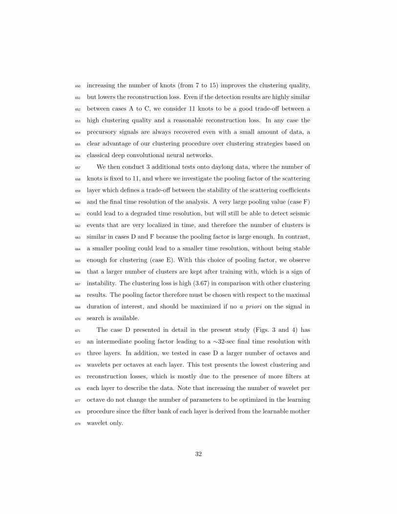
increasing the number of knots (from 7 to 15) improves the clustering quality,650

but lowers the reconstruction loss. Even if the detection results are highly similar651

between cases A to C, we consider 11 knots to be a good trade-off between a652

high clustering quality and a reasonable reconstruction loss. In any case the653

precursory signals are always recovered even with a small amount of data, a654

clear advantage of our clustering procedure over clustering strategies based on655

classical deep convolutional neural networks.656

We then conduct 3 additional tests onto daylong data, where the number of657

knots is fixed to 11, and where we investigate the pooling factor of the scattering658

layer which defines a trade-off between the stability of the scattering coefficients659

and the final time resolution of the analysis. A very large pooling value (case F)660

could lead to a degraded time resolution, but will still be able to detect seismic661

events that are very localized in time, and therefore the number of clusters is662

similar in cases D and F because the pooling factor is large enough. In contrast,663

a smaller pooling could lead to a smaller time resolution, without being stable664

enough for clustering (case E). With this choice of pooling factor, we observe665

that a larger number of clusters are kept after training with, which is a sign of666

instability. The clustering loss is high (3.67) in comparison with other clustering667

results. The pooling factor therefore must be chosen with respect to the maximal668

duration of interest, and should be maximized if no a priori on the signal in669

search is available.670

The case D presented in detail in the present study (Figs. 3 and 4) has671

an intermediate pooling factor leading to a ∼32-sec final time resolution with672

three layers. In addition, we tested in case D a larger number of octaves and673

wavelets per octaves at each layer. This test presents the lowest clustering and674

reconstruction losses, which is mostly due to the presence of more filters at675

each layer to describe the data. Note that increasing the number of wavelet per676

octave do not change the number of parameters to be optimized in the learning677

procedure since the filter bank of each layer is derived from the learnable mother678

wavelet only.679

32

Comparison of cluster detection rates and microseismic en-680

ergy681

We collect the spectral pressure calculated from the WAVEWATCH III model682

(CIET ARDHUIN) on a 0.5×0.5 degree grid globally, from 2017-06-01 to 2017-683

06-18. This pressure data cannot be directly used as a proxy for radiated seismic684

energy, because the radiation of body and surface waves depends on the bathy-685

metric profile of the seefloor [45]. According to [45], the equivalent radiated686

spectral energy can be derived from the pressure with taking into account the687

resonnance of the water column at each point of the grid as amplification factor.688

We therefore used the amplification model presented in [45], where the global689

bathymetry is taken into account. We then considered the source time func-690

tion of each points of a 4 × 4 degree grid, and correlated it with the temporal691

within-cluster detection. Because the pressure data is availble every 3 hours, we692

decimated the within-cluster detection on the same time basis.693

The correlation is tested for several frequency bands (0.1 to 0.2, 0.2 to 0.3,694

0.3 to 0.45 and 0.45 to 0.6) and seismic waves (P waves, S waves and Rayleigh695

waves). For each frequency band, the maximally correlated source time func-696

tion and seismic wave type is identified and represented in Fig. S2 and S3. In697

addition to the water-column resonnance amplifications, we also apply different698

corrections for the different seismic wave types. The P-wave spectral energy is699

corrected from the shadowing of the Earth’s core (no energy should be recorded700

between 104 and 140 degrees of epicentral distance). This first correction is ap-701

plied as a mask on the correlation coefficients between within-cluster detection702

rates and source time functions. For Rayleigh waves, we also took into account703

the strong attenuation effects of the crust heterogeneities at these frequencies.704

We here considered an exponentially decaying attenuation with distance, with705

a decay of 1/500 km−1.706

33

References707

[1] Bergen, K. J., Johnson, P. A., Maarten, V. & Beroza, G. C. Machine708

learning for data-driven discovery in solid earth geoscience. Science 363,709

eaau0323 (2019).710

[2] Obara, K., Hirose, H., Yamamizu, F. & Kasahara, K. Episodic slow slip711

events accompanied by non-volcanic tremors in southwest japan subduction712

zone. Geophysical Research Letters 31 (2004).713

[3] Perol, T., Gharbi, M. & Denolle, M. Convolutional neural network for714

earthquake detection and location. Science Advances 4, e1700578 (2018).715

[4] Ross, Z. E., Meier, M.-A., Hauksson, E. & Heaton, T. H. Generalized seis-716

mic phase detection with deep learning. arXiv preprint arXiv:1805.01075717

(2018).718

[5] Scarpetta, S. et al. Automatic classification of seismic signals at mt. vesu-719

vius volcano, italy, using neural networks. Bulletin of the Seismological720

Society of America 95, 185–196 (2005).721

[6] Esposito, A. M., D’Auria, L., Giudicepietro, F., Caputo, T. & Martini,722

M. Neural analysis of seismic data: applications to the monitoring of mt.723

vesuvius. Annals of Geophysics (2013).724

[7] Maggi, A. et al. Implementation of a multistation approach for automated725

event classification at piton de la fournaise volcano. Seismological Research726

Letters 88, 878–891 (2017).727

[8] Malfante, M. et al. Machine learning for volcano-seismic signals: Challenges728

and perspectives. IEEE Signal Processing Magazine 35, 20–30 (2018).729

[9] Esposito, A. et al. Unsupervised neural analysis of very-long-period events730

at stromboli volcano using the self-organizing maps. Bulletin of the Seis-731

mological Society of America 98, 2449–2459 (2008).732

34

00:00 03:00 06:00 09:00 12:00 15:00 18:00 21:00 00:000

50

100A

1 2 3 4

565

153

103

11

10 0 10

123

00:00 03:00 06:00 09:00 12:00 15:00 18:00 21:00 00:000

50

100B

1 2 3

679

126

27

10 0 10

123

00:00 03:00 06:00 09:00 12:00 15:00 18:00 21:00 00:000

50

100C

1 2 3

695

108

29

10 0 10

123

00:00 03:00 06:00 09:00 12:00 15:00 18:00 21:00 00:000

50

100D

1 2 3 4

151

4 7

11 1

71 3

610 0 10

123

00:00 03:00 06:00 09:00 12:00 15:00 18:00 21:00 00:000

50

100E

1 2 3 4 5 6

284

6 1

603

231

73

58

53

10 0 10

123

00:00 03:00 06:00 09:00 12:00 15:00 18:00 21:00 00:00Time on 2017-06-17

0

50

100F

1 2 3 4Clusters

population

102

9 8

3 7

8 2

6

10 0 10

1

2

3

10 0 10

1

2

3

G

Lear

ned

mot

her w

avel

et (a

t eac

h la

yer i

ndex

)

Cum

mul

ativ

e w

ithin

-clu

ster

det

ectio

n (n

orm

aliz

ed)

Figure S7: (Supplementary material) Learning results with different

parameters. The different parameter sets are given in Table 1. The left and

middle plots respectively show the within-cluster cumulative detections and the

within-cluster number of samples after 10,000 training epochs. The right plots

show the final learned wavelets at each layer. (A – F) results obtained with

the parameters sets given in Table 1, (D) being the case analyzed in details in

Fig. 3 and 4. (G) learned mother wavelet at each layer with all parameter sets.

35

Jun 03 05 07 09 11 13 15 172017-Jun

0.2

0.0

0.2

0.4

0.6

0.8

1.0

3-ho

urly

det

ectio

n ra

te

Correlation: 0.87, frequency band: 0.1 0.2 HzA

0.5

0.0

0.5

1.0

1.5

2.0

2.5

P-w

ave

spec

tral e

nerg

y (M

Pa/

m²/s

²)

-180° -120° -60° 0° 60° 120° 180°Longitude (degrees)

-90°

-45°

0°

45°

90°

Latit

ude

(deg

rees

)

B

0.0

0.2

0.4

0.6

0.8

1.0

Like

lihoo

d

Figure S8: (Supplementary material) Comparison of clusters D with

P-wave microseismic energy. (A) The whithin-cluster 3-hourly detection is

presented in red curve over 17 days of 3-components seismic data. The best-

matching radiated P-wave spectral energy in the frequency band 0.1 to 0.2 Hz is

presented in black line. (B) Global matching likelihood of the spectral P-wave

radiated energy between 0.1 and 0.2 Hz on a 4×4 degrees grid. The likelihood

is corrected for theoretical P-wave shadow zones due to the presence of the

core (between 104 and 140 degrees of epicentral distance), visible by the zero-

likelihood zone. The highest likelihood from which the source-time function is

extracted and presented in A is highlighted with a black circle in B.

36

Jun 03 05 07 09 11 13 15 172017-Jun

0.2

0.0

0.2

0.4

0.6

0.8

1.0

3-ho

urly

det

ectio

n ra

te

Correlation: 0.86, frequency band: 0.45 0.6 HzA

0.05

0.00

0.05

0.10

0.15

0.20

0.25

0.30

Ray

leig

h w

ave

spec

tral e

nerg

y (M

Pa/

m²/s

²)

-180° -120° -60° 0° 60° 120° 180°Longitude (degrees)

-90°

-45°

0°

45°

90°

Latit

ude

(deg

rees

)

B

0.0

0.2

0.4

0.6

0.8

1.0

Like

lihoo

d

Figure S9: (Supplementary material) Comparison of clusters C with

Rayleigh wave microseismic energy. (A) The whithin-cluster 3-hourly

detection is presented in purple curve over 17 days of 3-components seismic

data. The best-matching radiated Rayleigh-wave spectral energy in the fre-

quency band 0.45 to 0.6 Hz is presented in black line. (B) Global matching

likelihood of the spectral Rayleigh-wave radiated energy between 0.45 to 0.6 Hz

on a 4×4 degrees grid. The likelihood is corrected from theoretical Rayleigh

wave attenuation due to strong scattering at these frequencies. The highest

likelihood from which the source-time function is extracted and presented in A

is highlighted with a black circle in B.

37

[10] Unglert, K. & Jellinek, A. Feasibility study of spectral pattern recogni-733

tion reveals distinct classes of volcanic tremor. Journal of Volcanology and734

Geothermal Research 336, 219–244 (2017).735

[11] Hammer, C., Ohrnberger, M. & Faeh, D. Classifying seismic waveforms736

from scratch: a case study in the alpine environment. Geophysical Journal737

International 192, 425–439 (2012).738

[12] Soubestre, J. et al. Network-based detection and classification of seismo-739

volcanic tremors: Example from the klyuchevskoy volcanic group in kam-740

chatka. Journal of Geophysical Research: Solid Earth 123, 564–582 (2018).741

[13] Beyreuther, M., Hammer, C., Wassermann, J., Ohrnberger, M. & Megies,742

T. Constructing a hidden markov model based earthquake detector: ap-743

plication to induced seismicity. Geophysical Journal International 189,744

602–610 (2012).745

[14] Holtzman, B. K., Pate, A., Paisley, J., Waldhauser, F. & Repetto, D.746

Machine learning reveals cyclic changes in seismic source spectra in geysers747

geothermal field. Science advances 4, eaao2929 (2018).748

[15] Yoon, C. E., O’Reilly, O., Bergen, K. J. & Beroza, G. C. Earthquake detec-749

tion through computationally efficient similarity search. Science advances750

1, e1501057 (2015).751

[16] Mousavi, S. M., Zhu, W., Ellsworth, W. & Beroza, G. Unsupervised clus-752

tering of seismic signals using deep convolutional autoencoders. IEEE Geo-753

science and Remote Sensing Letters (2019).754

[17] Kohler, A., Ohrnberger, M. & Scherbaum, F. Unsupervised pattern recog-755

nition in continuous seismic wavefield records using self-organizing maps.756

Geophysical Journal International 182, 1619–1630 (2010).757

[18] Rouet-Leduc, B. et al. Machine learning predicts laboratory earthquakes.758

Geophysical Research Letters 44, 9276–9282 (2017).759

38

[19] Bruna, J. & Mallat, S. Invariant scattering convolution networks. IEEE760

transactions on pattern analysis and machine intelligence 35, 1872–1886761

(2013).762

[20] Anden, J. & Mallat, S. Deep scattering spectrum. IEEE Transactions on763

Signal Processing 62, 4114–4128 (2014).764

[21] Anden, J. & Mallat, S. Scattering representation of modulated sounds.765

15th DAFx 9 (2012).766

[22] Peddinti, V. et al. Deep scattering spectrum with deep neural networks.767

In Acoustics, Speech and Signal Processing (ICASSP), 2014 IEEE Inter-768

national Conference on, 210–214 (IEEE, 2014).769

[23] Balestriero, R., Cosentino, R., Glotin, H. & Baraniuk, R. Spline filters770

for end-to-end deep learning. In Dy, J. & Krause, A. (eds.) Proceedings of771

the 35th International Conference on Machine Learning, vol. 80 of Proceed-772

ings of Machine Learning Research, 364–373 (PMLR, Stockholmsmassan,773

Stockholm Sweden, 2018).774

[24] Ahuja, N., Lertrattanapanich, S. & Bose, N. Properties determining choice775

of mother wavelet. IEE Proceedings-Vision, Image and Signal Processing776

152, 659–664 (2005).777

[25] Meyer, Y. Wavelets and operators, vol. 1 (Cambridge university press,778

1992).779

[26] Coifman, R. R. & Wickerhauser, M. V. Entropy-based algorithms for best780

basis selection. IEEE Transactions on information theory 38, 713–718781

(1992).782

[27] Poli, P. Creep and slip: Seismic precursors to the nuugaatsiaq landslide783

(greenland). Geophysical Research Letters 44, 8832–8836 (2017).784

[28] Chao, W.-A. et al. The large greenland landslide of 2017: Was a tsunami785

warning possible? Seismological Research Letters (2018).786

39

[29] Bell, A. F. Predictability of landslide timing from quasi-periodic precursory787

earthquakes. Geophysical Research Letters 45, 1860–1869 (2018).788

[30] Allen, R. Automatic phase pickers: Their present use and future prospects.789

Bulletin of the Seismological Society of America 72, S225–S242 (1982).790

[31] Gibbons, S. J. & Ringdal, F. The detection of low magnitude seismic events791

using array-based waveform correlation. Geophysical Journal International792

165, 149–166 (2006).793

[32] Brown, J. R., Beroza, G. C. & Shelly, D. R. An autocorrelation method794

to detect low frequency earthquakes within tremor. Geophysical Research795

Letters 35 (2008).796

[33] Estivill-Castro, V. Why so many clustering algorithms: a position paper.797

SIGKDD explorations 4, 65–75 (2002).798

[34] Chakraborty, A. & Okaya, D. Frequency-time decomposition of seismic799

data using wavelet-based methods. Geophysics 60, 1906–1916 (1995).800

[35] Dumoulin, V. & Visin, F. A guide to convolution arithmetic for deep801

learning. arXiv preprint arXiv:1603.07285 (2016).802

[36] Shelly, D. R., Beroza, G. C. & Ide, S. Non-volcanic tremor and low-803

frequency earthquake swarms. Nature 446, 305 (2007).804

[37] Reynolds, D. Gaussian mixture models. Encyclopedia of biometrics 827–805

832 (2015).806

[38] Mallat, S. A wavelet tour of signal processing: the sparse way, chap. 4,807

111–112 (Elsevier, 2009), 3 edn.808

[39] Kingma, D. P. & Ba, J. Adam: A method for stochastic optimization.809

arXiv preprint arXiv:1412.6980 (2014).810

[40] Johnson, S. C. Hierarchical clustering schemes. Psychometrika 32, 241–254811

(1967).812

40

[41] Von Luxburg, U. A tutorial on spectral clustering. Statistics and computing813

17, 395–416 (2007).814

[42] Sifre, L., Kapoko, M., Oyallon, E. & Lostanlen, V. Scatnet: a matlab815

toolbox for scattering networks (2013).816

[43] Xu, L. & Jordan, M. I. On convergence properties of the em algorithm for817

gaussian mixtures. Neural computation 8, 129–151 (1996).818

[44] Ardhuin, F. et al. Ocean wave sources of seismic noise. Journal of Geo-819

physical Research: Oceans 116(C9) (2011).820

[45] Li, L., Boue, P. & Campillo, M. Spatiotemporal connectivity of noise-821

derived seismic body waves with ocean waves and microseism excitations822

Eartharxiv (2019).823

41