Embed Size (px)
Citation preview

ACCELERATING CHEMICAL SIMILARITY SEARCH USING GPUS
AND METRIC EMBEDDINGS
A DISSERTATION
SUBMITTED TO THE DEPARTMENT OF COMPUTER SCIENCE
AND THE COMMITTEE ON GRADUATE STUDIES
OF STANFORD UNIVERSITY
IN PARTIAL FULFILLMENT OF THE REQUIREMENTS
FOR THE DEGREE OF
DOCTOR OF PHILOSOPHY
Imran Saeedul Haque
September 2011

Abstract
Fifteen years ago, the advent of modern high-throughput sequencing revolutionized compu-
tational genetics with a flood of data. Today, high-throughput biochemical assays promise
to make biochemistry the next data-rich domain for machine learning. However, existing
computational methods, built for small analyses of about 1,000 molecules, do not scale
to emerging multi-million molecule datasets. For many algorithms, pairwise similarity
comparisons between molecules are a critical bottleneck, presenting a 1,000×-1,000,000×scaling barrier.
In this dissertation, I describe the design of SIML and PAPER, our GPU implementations
of 2D and 3D chemical similarities, as well as SCISSORS, our metric embedding algorithm.
On a model problem of interest, combining these techniques allows up to 274,000x speedup
in time and up to 2.8 million-fold reduction in space while retaining excellent accuracy. I
further discuss how these high-speed techniques have allowed insight into chemical shape
similarity and the behavior of machine learning kernel methods in the presence of noise.
iv

Acknowledgements
I offer a world of thanks to the people who have helped me through the process of graduate
school and the Ph.D. First and foremost, I thank my family: my parents Yusuf and Nilufar,
brothers Omar and Ejaz, and all the rest. Five years feels a lot longer in the middle of year
three; knowing that my family is local, understands the doctorate process, and is behind
me has been huge. (Grabbing the occasional home-cooked meal doesn’t hurt either.) In
particular, to my grandmother: you surely didn’t know, in the middle of my second year,
that I was doubting whether I had the chops to compete with all the sheer talent around me.
But after you said, “I’m so proud, three generations: first your grandfather with a Ph.D.,
then your father, and now you.” — there wasn’t any other way to go, was there? Thank you.
Thanks also to my friends, be they from my days at Stanford, Berkeley, Bellarmine,
Challenger, or even before. Staying in the Bay Area for so long has its advantages, and a
deep social network is definitely among them. Go Bells and go Bears!
When we get to the actual “work” part of this thesis, many thanks to my primary thesis
advisor, Vijay Pande. I could not have asked for a better advisor than Vijay; the care he shows
for his graduate students, whether it is reflected in the questions he asks at weekly meetings,
his encouragement of (seemingly distracting) side projects, the laissez-faire strategy for
working hours, or even simply his support for lab members working with modern computer
equipment, appear in both the happiness and productivity of the lab as a whole. Vijay, it’s
been a privilege to have worked with you. This applies equally to the rest of the Pande
group. Listing everyone would extend this section to ten pages. Suffice it to say that you all
have taught me that nothing in computational biochemistry works (but some things do); that
thermodynamics is equally applicable to protein folding and the tailgate preparation of roast
duck; that the wet lab is full of pain, but stepping away from the computer is a good idea;
v
and that even though it seems like our projects may be too many steps removed from the
real world, that it’s important to keep your eyes on the target.
Funding for my graduate work was provided in large part by a graduate research
fellowship from the National Science Foundation, so thanks to the American taxpayer
for considering science to be a worthy cause.
Oh, and finally: haters to the left. Thanks.
vi
Contents
Abstract iv
Acknowledgements v
1 Introduction 11.1 Computational Biochemistry . . . . . . . . . . . . . . . . . . . . . . . . . 2
1.2 Chemical Similarity . . . . . . . . . . . . . . . . . . . . . . . . . . . . . . 4
1.3 Modern Cheminformatics . . . . . . . . . . . . . . . . . . . . . . . . . . . 6
1.4 Outline and Reading Order . . . . . . . . . . . . . . . . . . . . . . . . . . 9
2 GPU Acceleration of 3D Chemical Shape Similarity 102.1 Introduction . . . . . . . . . . . . . . . . . . . . . . . . . . . . . . . . . . 11
2.2 ROCS: Rapid Overlay of Chemical Structures . . . . . . . . . . . . . . . . 12
2.2.1 Theory of Molecular Shape . . . . . . . . . . . . . . . . . . . . . 12
2.2.2 Optimization of Volume Overlap . . . . . . . . . . . . . . . . . . . 13
2.3 Implementing Shape Overlay on the NVIDIA G80 . . . . . . . . . . . . . 14
2.3.1 NVIDIA G80 GPU Architecture . . . . . . . . . . . . . . . . . . . 14
2.3.2 The CUDA Programming Language . . . . . . . . . . . . . . . . . 14
2.3.3 Mapping ROCS Computation to NVIDIA Hardware . . . . . . . . 16
2.3.4 Memory Layout . . . . . . . . . . . . . . . . . . . . . . . . . . . 17
2.4 Results . . . . . . . . . . . . . . . . . . . . . . . . . . . . . . . . . . . . . 18
2.4.1 Testing Methodology . . . . . . . . . . . . . . . . . . . . . . . . . 18
2.4.2 Accuracy vs oeROCS . . . . . . . . . . . . . . . . . . . . . . . . . 22
2.4.3 Virtual Screening Performance vs oeROCS . . . . . . . . . . . . . 28
vii

2.4.4 Speed vs cpuROCS . . . . . . . . . . . . . . . . . . . . . . . . . . 30
2.4.5 Speed vs oeROCS . . . . . . . . . . . . . . . . . . . . . . . . . . 32
2.5 Conclusions . . . . . . . . . . . . . . . . . . . . . . . . . . . . . . . . . . 38
2.6 Acknowledgments . . . . . . . . . . . . . . . . . . . . . . . . . . . . . . 40
2.7 Appendix: Rotational gradients for shape overlay . . . . . . . . . . . . . . 40
2.7.1 Gradient of volume V with respect to transform T . . . . . . . . . 41
2.7.2 Coordinate derivatives: ∇~χk(T ) . . . . . . . . . . . . . . . . . . . 42
3 GPU Acceleration of SMILES-based 2D Chemical Similarity 503.1 Introduction . . . . . . . . . . . . . . . . . . . . . . . . . . . . . . . . . . 51
3.2 Methods . . . . . . . . . . . . . . . . . . . . . . . . . . . . . . . . . . . . 52
3.2.1 Overview of LINGO . . . . . . . . . . . . . . . . . . . . . . . . . 52
3.2.2 Our Algorithm . . . . . . . . . . . . . . . . . . . . . . . . . . . . 53
3.2.3 GPU implementation . . . . . . . . . . . . . . . . . . . . . . . . . 54
3.3 Results . . . . . . . . . . . . . . . . . . . . . . . . . . . . . . . . . . . . . 57
3.3.1 Benchmarking Methodology . . . . . . . . . . . . . . . . . . . . . 57
3.3.2 Performance . . . . . . . . . . . . . . . . . . . . . . . . . . . . . 58
3.4 Analysis . . . . . . . . . . . . . . . . . . . . . . . . . . . . . . . . . . . . 60
3.5 Conclusions . . . . . . . . . . . . . . . . . . . . . . . . . . . . . . . . . . 61
4 Optimization of GPU Chemical Similarity 634.1 Introduction, Problem Statement, and Context . . . . . . . . . . . . . . . . 64
4.1.1 Gaussian shape overlay: background . . . . . . . . . . . . . . . . . 64
4.1.2 LINGO: background . . . . . . . . . . . . . . . . . . . . . . . . . 66
4.2 Core Methods . . . . . . . . . . . . . . . . . . . . . . . . . . . . . . . . . 68
4.3 Gaussian Shape Overlay: Parallelization and Arithmetic Optimization . . . 69
4.3.1 Evaluation of data-parallel objective function . . . . . . . . . . . . 70
4.3.2 Kernel fusion and CPU/GPU balancing . . . . . . . . . . . . . . . 74
4.4 LINGO — Algorithmic Transformation and Memory Optimization . . . . . 75
4.4.1 SIML GPU implementation and memory tuning . . . . . . . . . . 78
4.5 Final evaluation . . . . . . . . . . . . . . . . . . . . . . . . . . . . . . . . 79
4.6 Future Directions . . . . . . . . . . . . . . . . . . . . . . . . . . . . . . . 83
viii
4.7 Acknowledgments . . . . . . . . . . . . . . . . . . . . . . . . . . . . . . 83
5 SCISSORS: A Linear-Algebraical Technique to Rapidly Approximate Chemi-cal Similarities 845.1 Introduction . . . . . . . . . . . . . . . . . . . . . . . . . . . . . . . . . . 85
5.2 Method . . . . . . . . . . . . . . . . . . . . . . . . . . . . . . . . . . . . 86
5.2.1 Correction Factors . . . . . . . . . . . . . . . . . . . . . . . . . . 88
5.2.2 Fast approximation of new vectors . . . . . . . . . . . . . . . . . . 91
5.3 Results . . . . . . . . . . . . . . . . . . . . . . . . . . . . . . . . . . . . . 92
5.3.1 Similarity Measures . . . . . . . . . . . . . . . . . . . . . . . . . 92
5.3.2 Molecules Tested . . . . . . . . . . . . . . . . . . . . . . . . . . . 93
5.3.3 Basis size and dimensionality . . . . . . . . . . . . . . . . . . . . 94
5.3.4 Basis selection strategies . . . . . . . . . . . . . . . . . . . . . . . 94
5.3.5 Corrected Tanimotos . . . . . . . . . . . . . . . . . . . . . . . . . 97
5.3.6 Virtual screening . . . . . . . . . . . . . . . . . . . . . . . . . . . 98
5.3.7 Similarity measure generalizability . . . . . . . . . . . . . . . . . 100
5.3.8 Tanimoto Computation Speed . . . . . . . . . . . . . . . . . . . . 102
5.4 Discussion . . . . . . . . . . . . . . . . . . . . . . . . . . . . . . . . . . . 105
5.4.1 Connections to Previous Work . . . . . . . . . . . . . . . . . . . . 105
5.4.2 Interpretation of chemical similarities . . . . . . . . . . . . . . . . 108
5.4.3 Insights into chemical space . . . . . . . . . . . . . . . . . . . . . 111
5.4.4 Applications — Fast library screening and clustering with SCISSORS111
5.5 Conclusion . . . . . . . . . . . . . . . . . . . . . . . . . . . . . . . . . . 112
5.6 Appendix: Detailed Methods . . . . . . . . . . . . . . . . . . . . . . . . . 113
5.6.1 Molecular Databases and Preprocessing . . . . . . . . . . . . . . . 113
5.6.2 Software versions . . . . . . . . . . . . . . . . . . . . . . . . . . . 115
5.6.3 Software settings for similarity calculations . . . . . . . . . . . . . 115
5.6.4 Performance benchmarking setup . . . . . . . . . . . . . . . . . . 116
6 Error Bounds on SCISSORS 1186.1 Introduction . . . . . . . . . . . . . . . . . . . . . . . . . . . . . . . . . . 119
6.2 Preliminaries . . . . . . . . . . . . . . . . . . . . . . . . . . . . . . . . . 120
ix

6.2.1 SCISSORS as a kernel method . . . . . . . . . . . . . . . . . . . . 120
6.2.2 Assumptions . . . . . . . . . . . . . . . . . . . . . . . . . . . . . 122
6.3 Reduction of SCISSORS to Kernel PCA . . . . . . . . . . . . . . . . . . . 123
6.3.1 Overview of Kernel PCA . . . . . . . . . . . . . . . . . . . . . . . 123
6.3.2 Derivation of kernel PCA . . . . . . . . . . . . . . . . . . . . . . . 124
6.3.3 Reduction Proof . . . . . . . . . . . . . . . . . . . . . . . . . . . 125
6.4 Reduction of SCISSORS to the Nystrom Rank-k Approximation . . . . . . 126
6.4.1 Overview of the Nystrom Method . . . . . . . . . . . . . . . . . . 126
6.4.2 Preliminaries . . . . . . . . . . . . . . . . . . . . . . . . . . . . . 127
6.4.3 Final Reduction . . . . . . . . . . . . . . . . . . . . . . . . . . . . 129
6.5 Expected error in individual inner products is bounded with high probability 129
6.5.1 Statement of the theorem . . . . . . . . . . . . . . . . . . . . . . . 129
6.5.2 Proof Overview . . . . . . . . . . . . . . . . . . . . . . . . . . . . 130
6.5.3 Proof of Theorem 6.1 . . . . . . . . . . . . . . . . . . . . . . . . . 131
6.6 The error in SCISSORS-approximated Gram matrices is bounded in 2-norm,
Frobenius norm, and RMS deviation . . . . . . . . . . . . . . . . . . . . . 134
6.6.1 Statement of Theorems . . . . . . . . . . . . . . . . . . . . . . . . 134
6.6.2 Proof Overview . . . . . . . . . . . . . . . . . . . . . . . . . . . . 135
6.6.3 Proof of Theorems 6.3, 6.4, and 6.5 . . . . . . . . . . . . . . . . . 136
6.7 Conclusions . . . . . . . . . . . . . . . . . . . . . . . . . . . . . . . . . . 137
7 The Impact of Noisy Kernel Computation on Low-Rank Kernel Approxima-tion Methods 1387.1 Introduction . . . . . . . . . . . . . . . . . . . . . . . . . . . . . . . . . . 139
7.2 Past work and the origins of noise . . . . . . . . . . . . . . . . . . . . . . 140
7.3 Perturbing the spectral decomposition . . . . . . . . . . . . . . . . . . . . 142
7.4 First-order approximation to the kernel error . . . . . . . . . . . . . . . . . 146
7.5 Experiments . . . . . . . . . . . . . . . . . . . . . . . . . . . . . . . . . . 151
7.5.1 Noise floors . . . . . . . . . . . . . . . . . . . . . . . . . . . . . . 154
7.5.2 Increasing error . . . . . . . . . . . . . . . . . . . . . . . . . . . . 154
7.6 Practical Recommendations . . . . . . . . . . . . . . . . . . . . . . . . . . 156
x

7.7 Appendix 1: Detailed experimental methods . . . . . . . . . . . . . . . . . 158
7.7.1 Figure 7.1 . . . . . . . . . . . . . . . . . . . . . . . . . . . . . . . 158
7.7.2 LINGO calculations in Figures 7.2, 7.3 . . . . . . . . . . . . . . . 158
7.7.3 Shape calculations in Figures 7.2, 7.3 . . . . . . . . . . . . . . . . 159
7.7.4 Differential eigenspectrum plot . . . . . . . . . . . . . . . . . . . 159
7.8 Appendix 2: Proof that LINGO is a proper kernel . . . . . . . . . . . . . . 160
8 Real-Time 3D Chemical Similarity Search over PubChem 1618.1 Introduction . . . . . . . . . . . . . . . . . . . . . . . . . . . . . . . . . . 162
8.2 3D Similarity Measures . . . . . . . . . . . . . . . . . . . . . . . . . . . . 162
8.2.1 Shape . . . . . . . . . . . . . . . . . . . . . . . . . . . . . . . . . 163
8.2.2 Color . . . . . . . . . . . . . . . . . . . . . . . . . . . . . . . . . 164
8.3 GPU Implementation of 3D Color Similarity . . . . . . . . . . . . . . . . . 165
8.4 Fast Similarity Approximation by Metric Embedding . . . . . . . . . . . . 166
8.5 Materials and Methods . . . . . . . . . . . . . . . . . . . . . . . . . . . . 168
8.5.1 Databases . . . . . . . . . . . . . . . . . . . . . . . . . . . . . . . 168
8.5.2 Software . . . . . . . . . . . . . . . . . . . . . . . . . . . . . . . 168
8.5.3 SCISSORS Basis Sets . . . . . . . . . . . . . . . . . . . . . . . . 169
8.5.4 Evaluation Methodology . . . . . . . . . . . . . . . . . . . . . . . 169
8.6 Results: Parameter Selection . . . . . . . . . . . . . . . . . . . . . . . . . 170
8.7 Results: Accuracy . . . . . . . . . . . . . . . . . . . . . . . . . . . . . . . 171
8.8 Results: Throughput . . . . . . . . . . . . . . . . . . . . . . . . . . . . . 178
8.9 Conclusions . . . . . . . . . . . . . . . . . . . . . . . . . . . . . . . . . . 180
8.10 Acknowledgments . . . . . . . . . . . . . . . . . . . . . . . . . . . . . . 181
9 Conclusion and Future Directions 1829.1 Directions in Chemical Similarity Search . . . . . . . . . . . . . . . . . . 183
9.1.1 Reducing Noise in Shape Similarity . . . . . . . . . . . . . . . . . 183
9.1.2 Accelerating SCISSORS-based searches . . . . . . . . . . . . . . . 184
9.2 Topics in Kernel Methods . . . . . . . . . . . . . . . . . . . . . . . . . . . 185
9.3 Applications in Biochemical Machine Learning . . . . . . . . . . . . . . . 185
9.3.1 Fast One-vs-Many Search . . . . . . . . . . . . . . . . . . . . . . 186
xi

9.3.2 Fast Many-vs-Many Search . . . . . . . . . . . . . . . . . . . . . 186
9.3.3 Projecting Molecules into Vector Spaces . . . . . . . . . . . . . . . 187
xii

List of Tables
1.1 Runtime and storage requirements for a hypothetical BML method requiring
O(N2) time and space . . . . . . . . . . . . . . . . . . . . . . . . . . . . . 7
2.1 Hardware configurations tested for performance and accuracy benchmarking.
Systems without listed GPUs were used only for CPU-based (cpuROCS or
oeROCS) benchmarking. . . . . . . . . . . . . . . . . . . . . . . . . . . . 19
2.2 PAPER Initialization Modes Tested
(M ,N = # of cycle domains in query and fit) . . . . . . . . . . . . . . . . . 24
2.3 oeROCS performance in Exact mode. Times reported are time per alignment. 38
2.4 cpuROCS performance for Celeron 420. Times reported are time per align-
ment over all starting positions (“per alignment”) or per starting position
(“per start”). . . . . . . . . . . . . . . . . . . . . . . . . . . . . . . . . . . 44
2.5 cpuROCS performance for Xeon E5345. Times reported are time per align-
ment over all starting positions (“per alignment”) or per starting position
(“per start”) . . . . . . . . . . . . . . . . . . . . . . . . . . . . . . . . . . 45
2.6 cpuROCS performance for Athlon 64 X2 4800+. Times reported are time
per alignment over all starting positions (“per alignment”) or per starting
position (“per start”). . . . . . . . . . . . . . . . . . . . . . . . . . . . . . 45
2.7 PAPER performance for initialization mode 0 on selected batch sizes. Times
reported are time per alignment over all starting positions (“per alignment”)
or per starting position (“per start”). . . . . . . . . . . . . . . . . . . . . . 46
2.8 PAPER performance for initialization mode 1 on selected batch sizes. Times
reported are time per alignment over all starting positions (“per alignment”)
or per starting position (“per start”). . . . . . . . . . . . . . . . . . . . . . 47
xiii

2.9 PAPER performance for initialization mode 2 on selected batch sizes. Times
reported are time per alignment over all starting positions (“per alignment”)
or per starting position (“per start”). . . . . . . . . . . . . . . . . . . . . . 48
2.10 PAPER performance for initialization mode 5 on selected batch sizes. Times
reported are time per alignment over all starting positions (“per alignment”)
or per starting position (“per start”). . . . . . . . . . . . . . . . . . . . . . 49
3.1 Characteristics of SMILES sets from Maybridge used for benchmarking . . 58
3.2 Similarity matrix construction performance on CPU, 4,096 molecules, Ma-
chine 1 (parallel = 4 cores) . . . . . . . . . . . . . . . . . . . . . . . . . . 59
3.3 Similarity matrix construction performance on GPU. Times include transfer
of molecules to GPU and transfer of Tanimotos back to host. Note that total
work performed is quadratic in the number of molecules. . . . . . . . . . . 59
4.1 Effects of objective/gradient loop tuning on PAPER performance. Measured
on GTX 480 with “large” molecule set at 2000 molecules/batch. . . . . . . 74
4.2 Effects of kernel fusion on PAPER performance. Measured on GTX 480
with “large” molecule set at 2000 molecules/batch. . . . . . . . . . . . . . 75
4.3 Multiset vs. DFA algorithm performance on CPU, measured by calculating
an 8,192 × 8,192 LINGO similarity matrix on a Core i7-920. . . . . . . . . 77
5.1 SCISSORS precalculation step timings for 20,480 library molecules using
500 molecule basis set, using one core of a 3GHz Intel Xeon-based Mac Pro 105
xiv

List of Figures
1.1 Chapter dependency graph . . . . . . . . . . . . . . . . . . . . . . . . . . 9
2.1 Molecules used in PAPER performance testing . . . . . . . . . . . . . . . 23
2.2 Tanimoto scores for selected PAPER initialization modes (Y) vs oeROCS (X) 26
2.3 ROCS overlay errors with carbon-radius approximation . . . . . . . . . . . 27
2.4 Tanimoto scores of PAPER mode 2 vs mode 1 . . . . . . . . . . . . . . . . 27
2.5 ROC AUC values on each system of the DUD test set. Reported are the mean
AUC, averaged over each ligand in the system (line), the 68% confidence
interval on the AUC (box), and the 95% confidence interval on the AUC
(whiskers). Within each system, results are reported for for oeROCS in
exact (E) and grid (G) modes, and PAPER in initialization modes 0, 1, 2,
and 5 (labeled by mode number). oeROCS exact is highlighted in gray. . . 29
2.6 Systems for which PAPER performance varied significantly by initialization
mode. Reported are the mean AUC, averaged over each ligand in the
system (line), the 68% confidence interval on the AUC (box), and the 95%
confidence interval on the AUC (whiskers). Within each system, results are
reported for for oeROCS in exact (E) mode, highlighted in gray, and PAPER
in initialization modes 0, 1, 2, and 5 (labeled by mode number). . . . . . . 30
2.7 Systems for which PAPER performed significantly worse than oeROCS.
Reported are the mean AUC, averaged over each ligand in the system (line),
the 68% confidence interval on the AUC (box), and the 95% confidence
interval on the AUC (whiskers). Within each system, results are reported
for for oeROCS in exact (E) mode, highlighted in gray, and PAPER in
initialization modes 0, 1, 2, and 5 (labeled by mode number). . . . . . . . 31
xv

2.8 PAPER speedup vs cpuROCS: GTX 280 vs Xeon/icc . . . . . . . . . . . . 33
2.9 PAPER speedup vs cpuROCS: GTX 280 vs Athlon 64 X2/gcc . . . . . . . 34
2.10 PAPER speedup vs cpuROCS: 8800GTX vs Xeon/icc . . . . . . . . . . . . 35
2.11 PAPER speedup vs cpuROCS: 8800GTX vs Athlon 64 X2/gcc . . . . . . . 36
2.12 PAPER speedup vs cpuROCS: 8600GT vs Celeron/gcc . . . . . . . . . . . 37
2.13 PAPER speedup vs oeROCS: GTX 280 vs Athlon 64 3800+ . . . . . . . . 39
4.1 3D shape overlay of molecules. The reference and query molecules are
depicted as sticks (to visualize bond structure) embedded within their space-
filling representation. GSO rotates the query molecule to maximize its
volume overlap (blue spheres) with the volume of the reference (red mesh). 67
4.2 Chemical graph structure of a common solvent, its SMILES representation,
and its constituent Lingos. . . . . . . . . . . . . . . . . . . . . . . . . . . 67
4.3 Thread parallelization scheme in PAPER. Depicted is the full matrix of
interactions between a reference molecule of 11 atoms and a query molecule
of 17 atoms. Thread blocks of 32 threads process consecutive 32-element
strips of the matrix. Each color represents one iteration of a thread block.
Note that no more than a thread block-sized strip of matrix elements must
be materialized at any time during the computation. . . . . . . . . . . . . . 72
4.4 “Molecule-major” and “Lingo-major” layouts for storing the Lingos of
multiple molecules in memory. Red squares indicate the memory addresses
read by consecutive threads. “MX LY” indicates the Yth Lingo of the Xth
molecule. . . . . . . . . . . . . . . . . . . . . . . . . . . . . . . . . . . . 79
4.5 PAPER performance versus OpenEye ROCS . . . . . . . . . . . . . . . . . 82
4.6 SIML performance versus DFA-based LINGOs . . . . . . . . . . . . . . . 82
5.1 RMS Tanimoto error versus basis size and dimensionality of approxima-
tion for standard SCISSORS technique on ROCS Shape Tanimoto. 19000
library molecules (361M total Tanimotos) used to calculate RMSE. Each
bar averaged over at least 10 random bases of given size. . . . . . . . . . . 95
xvi

5.2 RMS Tanimoto error versus basis size and dimensionality of approximation
for standard SCISSORS technique on ROCS Shape Tanimoto. 50000 library
molecules (2500M total Tanimotos) used to calculate RMSE. Each bar
averaged over at least 10 random bases of given size. . . . . . . . . . . . . 96
5.3 RMS Tanimoto errors for SCISSORS approximations to ROCS shape Tani-
moto constructed from randomly-selected basis sets and basis sets chosen
by molecule clustering. All Tanimotos evaluated over 361M molecule pairs. 97
5.4 Density plots of SCISSORS and slack-corrected SCISSORS Tanimoto
approximations of ROCS Shape Tanimoto for 361M molecule pairs from
Maybridge. Contours are labeled as log10 of contour height. Light gray
y = x line drawn for reference. . . . . . . . . . . . . . . . . . . . . . . . . 99
5.5 ROC AUC values on each system of the DUD test set. Reported are the mean
AUC, averaged over each ligand in the system (line), the 68% confidence
interval on the AUC (box), and the 95% confidence interval on the AUC
(whiskers). Within each system, results are reported for ROCS (G, gray)
and SCISSORS using basis sets from the Maybridge Screening Collection
(M, red), the Asinex Screening Collection (A, orange), and the Maybridge
Fragment Library (F, blue). All SCISSORS approximations were done in
10 dimensions; Maybridge and Asinex sets used a 500-molecule basis set;
the Maybridge Fragment set was 473 molecules, the size of the entire library.101
5.6 RMS Tanimoto error from SCISSORS approximations to several molecular
similarity measures, as a function of dimensionality of approximation. All
tests conducted with basis size of 600 molecules and test set size of 1000
molecules. . . . . . . . . . . . . . . . . . . . . . . . . . . . . . . . . . . . 103
5.7 Eigenvalue spectra for Gram matrices resulting from four similarity mea-
sures on 1000 molecules from the M1 muscarinic data set . . . . . . . . . . 103
5.8 Interpretation of SCISSORS coordinates. All data from 128,371 Tanimotos
computed on DUD test set; 500 random molecules from Maybridge used as
basis. . . . . . . . . . . . . . . . . . . . . . . . . . . . . . . . . . . . . . 110
xvii

7.1 Histogram of the difference in kernel value for shape overlay computed
using 12 vs. 4 starting positions. An exact kernel would show no spread
away from zero difference. The computed standard deviation of 7.4 ≈ 5%
of the mean kernel value. . . . . . . . . . . . . . . . . . . . . . . . . . . . 141
7.2 Effects of kernel noise on Nystrom approximation . . . . . . . . . . . . . . 152
7.3 Eigenspectra and spectral gaps for noisy LINGO and shape . . . . . . . . . 155
8.1 Comparison of molecular structure and volume for benzene and pyridine . . 164
8.2 Basis vs Dimension RMS and mean error plots for SCISSORS on PLASTIC
and FastROCS Shape Tanimotos for PubChem3D . . . . . . . . . . . . . . 172
8.3 Basis vs Dimension RMS and mean error plots for SCISSORS on PLASTIC
and FastROCS Color Tanimotos for PubChem3D (all values) . . . . . . . . 173
8.4 Basis vs Dimension RMS and mean error plots for SCISSORS on PLASTIC
and FastROCS Color Tanimotos for PubChem3D (true Tanimoto > 0.5) . . 174
8.5 SCISSORS approximation based on PLASTIC and FastROCS Shape Tani-
motos: 256D, PC3DFP basis set . . . . . . . . . . . . . . . . . . . . . . . 175
8.6 SCISSORS approximation based on PLASTIC and FastROCS Color Tani-
motos: 192D PLASTIC, 256D FastROCS, PC3DFP basis set . . . . . . . . 176
8.7 SCISSORS combo Tanimoto approximation based on PLASTIC and Fas-
tROCS: Shape in 256D for both; color in 192D for PLASTIC and 256D for
FastROCS; PC3DFP basis set . . . . . . . . . . . . . . . . . . . . . . . . . 177
8.8 Histogram of change in true shape Tanimoto from using 12 starting points
rather than 4 with PAPER . . . . . . . . . . . . . . . . . . . . . . . . . . . 177
8.9 Density plot of PLASTIC color vs shape Tanimotos on PubChem3D evalua-
tion set . . . . . . . . . . . . . . . . . . . . . . . . . . . . . . . . . . . . . 177
xviii

Chapter 1
Introduction
Two major open problems in biochemistry are the ability to identify the proteins that will
bind an arbitrary small molecule in the cellular milieu as well as the converse problem of
finding compounds that would be bound by a particular protein. In various guises, these
fundamental questions underlie a large portion of drug discovery, toxicology, and chemical
biology in general. Target-based small molecule drug discovery (in which it is desired
to find a small molecule that activates or inhibits a known “target” protein) essentially
focuses around these two questions: finding an active compound is an instance of the latter
problem. Trying to predict the side effects and toxicity of a known compound is, at least in
part, a matter of discovering its possible “off-target” activities: other proteins to which the
compound binds whose activity is modulated thereby in a biologically-significant manner.
The most reliable methods to discover these activities are experimental: in vitro assays,
testing isolated compound and protein in solution; cellular assays testing compounds in
cells; in vivo animal screens; and human clinical trials. Because of the importance of
acquiring experimental protein binding data, significant improvements have been made
in recent years in high-throughput experimental techniques. Massively parallel methods
like high-throughput screening (usually using fluorescence or absorbance readouts in a 96-,
384-, or 1536-well plate format to quickly assay inhibitory potential) or highly-parallel
isothermal titration calorimetry (to directly measure the binding enthalpy and entropy) are
able to test hundreds to thousands of compounds simultaneously against a desired target
protein. Conversely, protein microarrays and bound-ligand affinity chromatography can
1
CHAPTER 1. INTRODUCTION 2
rapidly find proteins that will bind a particular compound with high affinity. Unfortunately,
experimental methods face problems of cost as well as sheer scale: assays require the use
of compounds and proteins that are often expensive and/or hard to synthesize/express, and
assay cost and time (on a per compound-protein pair basis) rises exponentially going from
in vitro to cellular, animal, and human testing. Furthermore, with thousands of known
proteins and over 35 million purchasable compounds, exhaustive experimental validation of
all possible binding pairs is not possible. It is also unnecessary: typical high-throughput
screens show that only a small fraction of compounds will actually inhibit a typical target at
reasonable concentration.
1.1 Computational Biochemistry
The high expense and labor-intensive nature of experimental biochemistry motivates compu-
tational approaches to the problem. One promising avenue is the use of physical simulation
to predict binding affinity. Free energy perturbation methods using molecular dynamics
[19, 80] or Monte Carlo [23, 50] techniques to sample the thermodynamic protein-ligand
binding partition function have shown success in estimating the binding affinity for a variety
of protein-ligand systems. However, such methods are extremely computationally intensive,
often taking days or weeks of supercomputer time to simulate even “easy” systems with
little protein flexibility. Furthermore, it is not clear whether current molecular dynamics
force fields and solvation models would even yield correct answers in the limit of infinite
computer time (in particular, the treatment of polarizability in most current forcefields is
weak) [52, 69]. The key reason for the expense of physical simulation is that it tries to
make an affinity prediction from physics alone, without harnessing related experimental
data (except indirectly through forcefield parameterization).
Consequently, it is of interest to consider computational methods to address the protein-
ligand binding question that are cheaper than full physical simulation. The field of chemical
informatics (also known as cheminformatics or chemoinformatics), studies ways to organize
and search chemical information, such as structures and assay data. In particular, a subfield
of cheminformatics, which I will term “biochemical machine learning,” or BML, seeks to
build models from existing experimental data to predict the results of future related assays

CHAPTER 1. INTRODUCTION 3
using statistical and machine learning methods. When cast in the language of data mining,
the biochemical learning problem is the following: we are given a matrix with proteins
along the rows and compounds along the columns in which each element is the binding
affinity (or inhibitory concentration, etc.) between that pair. Training data in this matrix are
only sparsely available (i.e., experimental values cover a very small subset of all possible
protein-ligand pairs) and are expensive to obtain; we would like to use a learning method to
predict the remaining entries.
A number of specific problems in biochemical machine learning, frequently treated in
the literature, can be expressed as variants of this problem. For example, in ligand-based
virtual screening, a number of compounds are known to be active against a particular target;
a large database of compounds is then queried for compounds hypothesized to be active
based on this training information. In the matrix formulation, this would be a query in
which a few elements are known in a given row, and we would like to predict the remainder.
Prediction of off-target activities is the transpose of this problem: here, we know one or a
few proteins to which our compound binds, and would like to predict other unknown binding
partners in the same column. Higher-order methods can be constructed by considering
more than one row or column in isolation; for example, one might use the fact that some
compounds show correlated activity on many proteins to predict that they should share
activities on a new protein.
BML, broadly speaking, can be divided into “structure-based” and “ligand-based” tech-
niques; in the former, structural information about both the protein target as well as the
chemical compound in question are available, whereas the latter uses only information
about the compounds. Structure-based techniques, such as docking, are often able to use
physics-based predictor functions [26, 43]. However, they are unusable for problems lacking
a solved protein structure or those for which the protein mediating a physical effect of
interest is unknown. Ligand-based methods, in contrast, require no protein information, but
cannot bring as much physical detail to bear. Rather, almost all ligand-based techniques
fundamentally rely on a hypothesis of similarity: that compounds which are “similar” ac-
cording to some measure will exhibit similar biological activity. Therefore, the definition
and evaluation of chemical similarity is essential to the practice of biochemical machine
learning [64].

CHAPTER 1. INTRODUCTION 4
1.2 Chemical Similarity
Broadly speaking, chemical similarity methods can be classified into three categories:
property-based, two-dimensional (2D), and three-dimensional (3D). From a machine learn-
ing standpoint, each class of similarity method can be interpreted as using a different set of
features defined on compounds. Property-based methods use as compound features various
physical properties of the molecule: for example, molecular weight, polar surface area, log
octanol-water partition coefficient (logP, a measurement of water solubility), or number of
rotatable bonds. While historically important to the development of cheminformatics, purely
property-based descriptors play a relatively minor role today except in particular specialties
(for example, in predicting membrane permeability [72]). Such methods are also often used
as negative controls in evaluating newer similarity techniques: it is expected that improved
similarity techniques ought to be able to outperform simple molecular weight thresholds,
for example.
2D similarity measures consider as features various properties of the chemical graph
of a compound. The chemical graph is a graph with vertices defined by atoms and edges
corresponding to interatomic bonds. Various properties can be associated with vertices:
typically, atom name (carbon, nitrogen, etc.), atom type (defined by particular force fields,
but may include atomic orbital hybridization information), and charge state. Edges also
have properties: most importantly, bond order defines the number of electron pairs shared in
that bond (1, 2, or 3), and additional properties such as bond aromaticity or resonance may
also be stored.
Different 2D methods are distinguished by their way of processing the chemical graph
to yield features. Fixed-substructure fingerprints, such as MDL keys [25], define for each
molecule a feature vector as a fixed-length binary vector. Each bit in this vector corresponds
to the presence or absence of a particular subgraph in the compound. The fixed set of
subgraph queries makes these methods both inflexible and insensitive: new chemical matter
containing subgraphs not present in the fingerprint set will not be well-mapped onto the
feature space.
Hashed substructure fingerprints, such as the extended-connectivity fingerprint (ECFP)
family [74], take a different approach. Rather than checking for the presence or absence
CHAPTER 1. INTRODUCTION 5
of predefined subgraphs, these methods enumerate all subgraphs present in the molecule,
under certain constraints. For example, ECFPx, for a positive integer x, considers around
each atom the x-bond-radius subgraph around that atom. Each subgraph is then hashed into
a very large binary vector, which is then reduced to a smaller (order of 1-4 kbit) vector by
“folding” (recursive binary-OR reduction). Hashed fingerprints gain flexibility at the cost of
interpretability, as individual fingerprint bits can no longer be unambiguously associated
with particular chemical features. Nevertheless, the use of 2D fingerprints for chemical
machine learning is widespread. Evaluation of 2D similarity is very fast (especially once
fingerprints have been precomputed). 2D graph analysis also aligns well with intuition over
chemical structures and reactions, which are often understood as graph transformations (e.g.,
subgraph augmentation or deletion in adding/removing functional groups).
While broadly used, 2D methods abstract away the physical reality of molecules by
considering only their atomic connectivity graphs. Molecules exist as three-dimensional
arrangements of atoms in space and this geometry is important to their activity. Recognizing
this, various methods exist to measure this similarity. Atom-distance methods are purely
geometric, considering the distribution of distances among atom pairs (or higher-order
tuples) or various descriptors of the overall molecular shape, such as maximum internal
lengths [5, 48, 76]. Field-based methods define the molecule as a scalar density field in
3-dimensional space (with density defined by van der Waals volume, electrostatic potential,
or proximity to a particular desired chemical feature) and compute similarity between
molecules as a functions between a pair of fields [18, 21, 33]. Finally, surface similarity
techniques consider only the similarity of compounds (e.g., in terms of sterics, hydrogen
bonding, and electrostatics) at their molecular surfaces [46]. 3D methods are an attempt
to model more faithfully the physical factors behind protein-ligand binding (such as steric
exclusion and electrostatic complementarity). However, as a consequence, they are often
much slower to evaluate than 2D similarities, with individual similarity evaluations taking
on the order of milliseconds to seconds, rather than nanoseconds to microseconds for 2D
similarities on precomputed fingerprints.

CHAPTER 1. INTRODUCTION 6
1.3 Modern Cheminformatics
An emerging trend in chemical informatics is the public availability of very large databases
of chemical structures and biochemical assay data. While pharmaceutical companies have
long had extensive databases of internal assay data and compound libraries, recent efforts
have begun to release large amounts of data to the public domain. The PubChem project
from the US National Center for Biotechnology Information (NCBI) holds, at the time
of writing, data from more than 34,000 assays, testing over 960,000 compounds. On a
similar scale, ChEMBLdb from the European Bioinformatics Institute has data on more
than 8,000 protein targets and 600,000 compounds. While much of the data comes from
publicly-funded ventures (such as the US National Institutes of Health Molecular Libraries
Screening Centers Network) and academic labs, private companies have also begun to
release significant amounts of data to the public. Perhaps the most prominent example to
date has been the release by GlaxoSmithKline of structures and assay data on thousands of
compounds hoped to be useful in the development of novel antimalarials [29].
The size of unlabeled chemical databases (i.e., those without assay information) has
also dramatically risen. NCBI’s PubChem3D database contains descriptors and computed
3-D structures for, at the time of writing, over 17 million compounds. The ZINC database
[45] contains structures with protonation states computed for various pH conditions for
approximately 35 million compounds claimed to be purchasable by their vendors. Con-
tinuing increases in computer power have inspired databases with even larger ambitions.
The GDB-13 [8] database, containing around 109 compounds, claims to enumerate all
“reasonable” chemical structures of 13 heavy (non-hydrogen) atoms or fewer containing a
restricted subset of atoms often found in organic chemistry; even larger so-called “generated”
or exhaustive databases have been proposed. Also in use are combinatorial databases, which
are able to contain 1012 or more compounds implicitly by specifying a chemical scaffold and
sets of possible transformations which create a combinatorially-large space of possibilities.
Ultimately, it is believed that the size of the synthesizable chemical universe under 30 heavy
atoms may be in the vicinity of 1060 compounds [9].
Unfortunately, computational methods in biochemistry have not kept pace with the
accelerating pace of experimental data acquisition. Many analysis methods were originally

CHAPTER 1. INTRODUCTION 7
developed to handle datasets on the 1,000 to 10,000 molecule scale — a very reasonable size
for dealing with single assays. Recent work has examined the similarity network structure
of a 400,000 compound subset of ZINC [84]. However, to achieve this, the authors had
to use computationally-inexpensive 2D similarity measures, use random subsampling, and
limit the scope of their analysis (in particular, no attempt was made at machine learning
for ligand activity). Even this work, at the limit of the computational capability in the field,
considers a number of compounds less than half the number of compounds with at least one
assay annotation in PubChem; it is orders of magnitude smaller than unlabeled databases
like PubChem3D or ZINC. There is a 10-100× gap in the size of computational analyses
that have been performed, and the size of databases that are already available (and growing).
The true gap in computational capability is much worse than the 10-100 fold number
would indicate; many methods of interest scale supralinearly in both time and space. For
example, methods that build graphical models based on the pairwise similarity network on a
set of compounds scale approximately as O(N2) in time and space, due to the requirement
to compute, histogram, and threshold the similarity matrix on compounds to set statistically-
relevant cutoffs on edges. A 10-100 fold gap inN implies that our computational capabilities
are 102-104 fold too weak to handle such quadratic-scaling problems.Table 1.1 shows the
approximate runtime and storage requirements of such a hypothetical method, based on the
ability to evaluate 100,000 pairwise compound similarities per second. Of particular note
is that storage becomes a serious concern for such methods. At the ten million molecule
scale, runtime is 3 CPU-yr, which is easily achieved on a cluster of modest size; however,
the required petabyte of storage is prohibitive with 2011-era technology. The GDB13-scale
billion-molecule database is impossible from both runtime and storage standpoints.
Problem size CPU time Storage needed10 mols 1 ms 1 kB
10K mols 1 min 1 GB100K mols 1 day 1 TB10M mols 3 yr 1 PB1B mols 30K yr 10K PB
Table 1.1: Runtime and storage requirements for a hypothetical BML method requiringO(N2) time and space

CHAPTER 1. INTRODUCTION 8
For many biochemical machine learning methods, the evaluation of pairwise ligand
similarities is a critical bottleneck. The example method of table 1.1 considered only
the runtime of similarity computations, ignoring the cost of model training, and already
was prohibitive on modern datasets. Furthermore, many similarity measures of interest,
particularly 3D similarities, are much slower than hypothesized in the table. ROCS, a
widely-used 3D similarity method developed by OpenEye Scientific Software, can compute
∼100-1000 similarities per second — thousands of times slower than assumed in the table.
For this reason, improving the performance of chemical similarity computation is of critical
importance to scaling machine learning to handle modern-scale biochemical data sets.
In this dissertation, I demonstrate that a two-pronged approach combining special-
purpose hardware with approximation algorithms is able to solve this scaling challenge for
an interesting subset of similarity measures. In the first half of the approach, I exploit the
massive parallelism of modern programmable graphics processors (GPUs) to accelerate
direct evaluation of both 3D and 2D similarity measures (chapters 2, 3, and 4), achieving
30-100× speedup. The second half of the strategy involves the development of a metric
embedding algorithm named SCISSORS, described in chapter 5. SCISSORS is used to
embed molecules into a real vector space such that similarity evaluations in this vector
space are a good approximation for the original similarity scores. Importantly, in chapter
8 it is demonstrated that this embedding can be performed in effectively linear time even
for a very large library like PubChem3D. Similarity computations in the embedded space
are so fast that the time for full pairwise comparison is dominated by the embedding
cost, yielding a final speedup from embedding alone on the order of 1000×. In chapter
8, I demonstrate that GPU acceleration forms an excellent complement to the embedding
method: the GPU-accelerated approximate similarity presented there is over 250,000×faster at a PubChem3D-scale O(N2) problem than the original technique. The combination
is so fast that it effectively solves the storage problem as well as the computation problem;
for both 2D and 3D similarities, the techniques described in this thesis can recompute the
O(N2) similarity matrix from O(N ) stored data faster than the similarity matrix could be
read back by a reasonable disk array, obviating the need to store a quadratic amount of data.
CHAPTER 1. INTRODUCTION 9
Chapter 3:GPU 2D Similarity
Chapter 4:GPU Optimization
Chapter 2: GPU 3D Similarity
Chapter 8:Real-time Search
Chapter 7:Noisy Kernels
Chapter 5:SCISSORS Intro
Chapter 6:SCISSORS Bounds
GPU Acceleration Metric Embedding
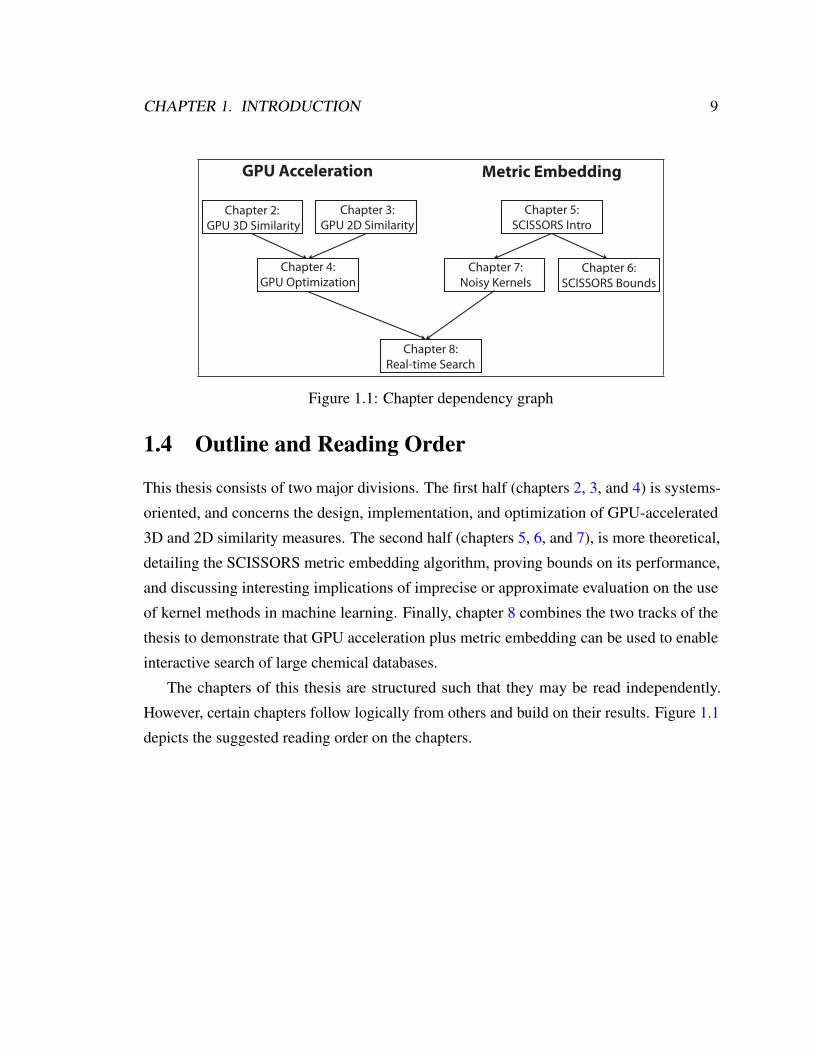
Figure 1.1: Chapter dependency graph
1.4 Outline and Reading Order
This thesis consists of two major divisions. The first half (chapters 2, 3, and 4) is systems-
oriented, and concerns the design, implementation, and optimization of GPU-accelerated
3D and 2D similarity measures. The second half (chapters 5, 6, and 7), is more theoretical,
detailing the SCISSORS metric embedding algorithm, proving bounds on its performance,
and discussing interesting implications of imprecise or approximate evaluation on the use
of kernel methods in machine learning. Finally, chapter 8 combines the two tracks of the
thesis to demonstrate that GPU acceleration plus metric embedding can be used to enable
interactive search of large chemical databases.
The chapters of this thesis are structured such that they may be read independently.
However, certain chapters follow logically from others and build on their results. Figure 1.1
depicts the suggested reading order on the chapters.

Chapter 2
GPU Acceleration of 3D Chemical ShapeSimilarity
Abstract
Modern graphics processing units (GPUs) are flexibly programmable and have peak com-
putational throughput significantly faster than conventional CPUs. Herein, we describe
the design and implementation of PAPER, an open-source implementation of Gaussian
molecular shape overlay for NVIDIA GPUs. We demonstrate one to two order-of-magnitude
speedups on high-end commodity GPU hardware relative to a reference CPU implementa-
tion of the shape overlay algorithm and speedups of over one order of magnitude relative
to the commercial OpenEye ROCS package. In addition, we describe errors incurred by
approximations used in common implementations of the algorithm.
This chapter (excluding appendices) has appeared previously in reference [39].
10

CHAPTER 2. GPU CHEMICAL 3D SIMILARITY 11
2.1 Introduction
Molecular shape comparison is a technique that identifies common spatial features among
two or more molecules and can be used as a similarity measure for ligand-based compound
discovery efforts. A popular technique of shape comparison, implemented in the ROCS [73]
package from OpenEye Scientific Software, applies the technique of Gaussian volume
overlap optimization [33] to perform a robust and fast shape overlay. ROCS is used
extensively in compound discovery and screening library development efforts [4, 37, 75, 82].
However, even with the efficiency of the Gaussian optimization technique, ROCS can take a
very long time to run when scanning over large compound sets, as in virtual high-throughput
screening. OpenEye’s support for PVM (Parallel Virtual Machine) clusters in its ROCS
software demonstrates that such screening with conventional ROCS is too slow to be carried
out on single computers. Therefore, new methods to accelerate ROCS-style alignment
should be useful for large-scale screening studies.
Recent trends in computer architecture have shifted the balance and nature of compu-
tational power on commodity desktops. The GeForce 8 series and Radeon X1000 series
of graphics cards from NVIDIA and AMD changed the conventional model of graphics
processing units (GPUs) — whereas GPUs began as task-specific engines for 3D rendering,
modern graphics cards are general, extremely-parallel computational engines. The CUDA
and CAL initiatives from NVIDIA and AMD, respectively, have made GPUs programmable
without the use of graphics-specific programming languages. On many measures includ-
ing peak FLOPS (floating-point operations per second), FLOPS per watt, and memory
bandwidth, modern GPUs outperform top-of-the-line CPUs on workloads that map well to
their parallelism, making GPU ports of conventional codes attractive from a performance
perspective.
In this article we describe PAPER (“PAPER Accelerates Parallel Evaluations of ROCS”),
an open-source implementation of ROCS’s Gaussian volume overlap optimization on
NVIDIA GPUs, available for download at https://simtk.org/home/paper/. We
begin with an overview of Gaussian overlap optimization (Section 2.2.2). We continue with
a description of the NVIDIA G80 architecture and the design decisions involved in imple-
menting ROCS-style optimization on such hardware in Section 2.3. Finally, we examine

CHAPTER 2. GPU CHEMICAL 3D SIMILARITY 12
the performance of our implementation. We highlight errors caused by algorithmic approx-
imations made by ROCS (Section 2.4.2). Furthermore, we demonstrate virtual screening
performance comparable to that of OpenEye ROCS (Section 2.4.3). Finally, we show one to
two order-of-magnitude speedups relative to a CPU implementation of our program (Section2.4.4), and speedups of over one order-of-magnitude relative to OpenEye ROCS (Section2.4.5).
2.2 ROCS: Rapid Overlay of Chemical Structures
2.2.1 Theory of Molecular Shape
The volume overlap between a pair of molecules A and B can be expressed as a product
integral between density functions representing the two molecules, where the integral is
taken over all space: ∫drρAρB (2.1)
These molecular density functions can be constructed from the density functions for the
component atoms 1...N by the relation
ρA(r) = 1−N∏i=1
(1− ρAi(r)) (2.2)
or, by the principle of inclusion-exclusion, as the following series of summations, which
account for overlaps between atoms:
ρA(r) =∑i
ρAi −∑i<j
ρAiρAj +∑i<j<k
ρAiρAjρAk
−∑
i<j<k<l
ρAiρAjρAkρAl + · · · (2.3)
The simplest definition of these atomic density functions ρAi sets them to 1 inside the
van der Waals radius of atom i, and 0 outside. Such a “hard-sphere” model is conceptually

CHAPTER 2. GPU CHEMICAL 3D SIMILARITY 13
simple, but has the disadvantage of being nondifferentiable, and therefore not amenable
to numeric optimization techniques. Although analytic hard-sphere models have been
developed [21], their complexity hinders performance. For this reason, Grant and Pickup
[35] proposed representing each atom as a spherical Gaussian function:
ρAk(r) = pk exp(−αk||rk − r||2
)(2.4)
Such Gaussian functions are smooth and differentiable. Furthermore, simple closed-form
expressions for the volumes, volume gradients (with respect to position), and Hessians of
the product of an arbitrary number of such Gaussians are known [35].
2.2.2 Optimization of Volume Overlap
Our optimization procedure largely follows the prescriptions from the original paper de-
scribing Gaussian volume overlap optimization [33], including the parameters defining the
atomic Gaussians: we set pi = 2√
2 and
αi =
π(3√
2
2π
) 23
r−2i
where ri is the van der Waals radius of atom i.
We parameterize the rigid-body transformation as a vector in <7, composed of a 3-
dimensional translation and a 4-dimensional quaternion. The quaternion component parame-
terizes the rotation as in the work of Griewank et al. [36]. It is restrained to unity magnitude
by a penalty term described by Kearsley[51], which resembles a Lagrange-multiplier tech-
nique, but with a fixed multiplier. We calculate both the overlap function and its gradient
with respect to the transformation coordinate, and optimize the molecular overlap using a
BFGS method [70] reimplemented for parallel execution on the GPU.
Because BFGS is a local optimizer, the starting configurations affect whether or not a
global optimum is reached. We initialize starting states similarly, but not identically, to the
Grant et al. method [33]. Unlike ROCS, we do not calculate shape centroids and multipoles
to determine starting positions and orientations. We determine the starting origin by an
CHAPTER 2. GPU CHEMICAL 3D SIMILARITY 14
arithmetic mean of all atom centers. The base orientation for each molecule is calculated
by rotating the molecule into the axes determined by the singular value decomposition of
the point cloud comprised by the atom centers. This SVD is equivalent (for non-degenerate
cases) to calculating the principal component axes of the atom centers.
Although the ROCS documentation claims that 4 starting coordinates are sufficient
to reach global optima [73], we have found (and discuss below) several cases in which
this is not true. This is a known problem — Grant et al. found cases requiring the use of
Monte Carlo optimization [33], and a more recent shape similarity paper [62] explains that
ROCS uses extra starting positions especially for molecules of high symmetry. We therefore
support multiple methods for generating initial configurations, including both deterministic
and randomized sampling of starting configurations, with varying sampling resolution.
2.3 Implementing Shape Overlay on the NVIDIA G80
2.3.1 NVIDIA G80 GPU Architecture
The NVIDIA G80 architecture, underlying all GeForce 8 and 9 series graphics cards, and a
derivative of which (GT200) underlies the GTX 200 series, is based on a “scalable processor
array” which can simultaneously execute up to 128 threads [55]. At a high level, the GPU is
structured as a number of TPCs (texture/processor clusters), each containing 2 (in G80) or 3
(in GT200 [86]) SMs (streaming multiprocessors). Each SM consists of 8 single-precision
floating point cores and 2 special-function units (SFUs) to handle transcendental operations.
Each SM also contains its own 16KiB of fast “shared memory”, which can be treated as a
user-controlled cache for the much larger “global memory” on the graphics card, and several
thousand (8192 on G80, 16384 on GT200) registers.
2.3.2 The CUDA Programming Language
CUDA [63] is a C-like programming language developed by NVIDIA to run general-purpose
computation on their G80 and newer graphics hardware. Following closely the structure
of the NVIDIA hardware, the CUDA execution model allows the execution on the GPU
of massively-multithreaded “kernels”, or GPU programs. The threads of each kernel are

CHAPTER 2. GPU CHEMICAL 3D SIMILARITY 15
arranged into thread blocks such that each block executes on exactly one SM (streaming
multiprocessor) on the hardware. Furthermore, each thread block has exclusive use of a
programmer-specified amount (up to the 16 KiB limit) of shared memory on its SM. Multiple
thread blocks may be assigned to the same SM if shared memory and register allocation
permit, in which case the SM time-slices between the blocks to hide latency from memory
access and instruction dependence.
CUDA’s memory model also reflects the structure of the underlying hardware, and this
structure is crucial for extracting maximum performance from the language. The fastest
storage is the register file in each SM, which is allocated on a per-thread basis (so that the
total number of registers used by a kernel equals the number of registers required per thread
times the number of threads per block). Next is the shared memory, which is local to each
thread block, and can be used for inter-thread communications. Shared memory is divided
into banks, such that under certain addressing restrictions, all threads can simultaneously
read from or write to shared memory. The largest and slowest memory is the main memory
on the graphics card, which CUDA splits into four categories:
• “Global memory” is general storage which is accessible to all threads and blocks of
the GPU program, but with a significant latency (hundreds of clock cycles), and which
can only reach its maximum bandwidth if accessed coherently (addressed sequentially
within blocks).
• “Local memory” is thread-local storage used to handle situations in which there are
insufficient registers on the SM to execute the kernel. Like global memory, it has high
latency.
• “Texture memory” describes read-only portions of global memory bound to special
pointers; special hardware exists on-chip to cache reads from texture memory, and to
do simple linear (or bi- or trilinear, for 2D and 3D textures) interpolation on texture
values. This hardware allows efficient implementation of lookup tables in texture
memory.
• “Constant memory” is a cached read-only portion of the device memory. Reads from
this constant cache are as fast as register reads, if all threads in a warp (the scheduling

CHAPTER 2. GPU CHEMICAL 3D SIMILARITY 16
unit on the hardware) read from the same address; otherwise the latency increases
linearly with the number of addresses read.
The primary way of loading data into a kernel from the host (CPU) side, or to bring
results back from a kernel execution, is to copy it between system memory and preallocated
space in the device global memory. However, because such a copy operation has relatively
low bandwidth (around 1GiB/s) and significant latency (tens of microseconds), minimizing
the number of GPU-CPU or CPU-GPU transfers is critical for maximizing performance.
2.3.3 Mapping ROCS Computation to NVIDIA Hardware
The CUDA programming model maps best to workloads that can be processed by many (hun-
dreds to thousands) of independent blocks of threads, with a large amount of computation
taking place on the GPU before more data is required from the CPU. Our implementation
moves almost all of the ROCS algorithm onto the GPU to best meet these objectives.
We have designed PAPER for the case in which many molecules are compared against
a single query molecule. This case can be expected to be common in virtual screening,
in which a library may be scanned for similarity to one or a few actives. The SVD-based
preprocessing of the molecules (Section 2.2.2) is handled externally in a Python script, as
the results of the preprocessing are easily stored on disk and need not be repeated for every
optimization.
In PAPER, the CPU first loads the molecules and then transforms them to an internal
data format. Since the algorithm we implement uses a local optimizer, the use of multiple
starting positions is important to find the global maximum in overlap. However, each of
these molecule-position pairs is a completely independent optimization problem. Therefore,
we make multiple copies of each molecule other than the query (the “fit” molecules) and
transform each into its unique starting orientation. This input data (the query molecule, the
copies of the fit molecules, and the starting coordinates corresponding to each transformed
copy) are copied in bulk to the GPU, making it possible to do hundreds of ROCS-type
optimizations in batch between CPU-GPU transfers, thereby minimizing transfer overhead.
PAPER maps the optimization onto the GPU in a manner designed to maximize the
parallelism accessible. Although the GPU offers thousands of threads worth of parallel

CHAPTER 2. GPU CHEMICAL 3D SIMILARITY 17
processing, no single ROCS calculation has that much parallelism. Therefore, we run
multiple calculations simultaneously — each molecule-orientation pair, as an independent
problem, is mapped to a separate CUDA thread block.
Hardware resources used by the GPU are allocated in units of “warps”: a warp corre-
sponds to a number of threads that run simultaneously on an SM (32 on current NVIDIA
hardware). If a given thread block has a number of threads which is not a multiple of
the warp size, hardware resources are wasted. Since each thread block should contain at
least one warp’s worth of threads to fully utilize the hardware, but the use of more threads
increases register pressure (thereby decreasing the number of blocks that can share an SM),
we use 64 threads per block. This means that each molecule-orientation pair has its own 64
threads on the GPU.
Once the optimizations are completed in parallel on the GPU, PAPER reads the final
overlap values and transformation coordinates back to system memory, and scans over each
molecule-orientation pairing to find the orientation for each molecule that produced the
maximum overlap. This is a relatively fast operation that can be efficiently performed on the
CPU.
2.3.4 Memory Layout
In order to minimize the impact of global memory latency on the PAPER kernel, we arrange
all data in global memory such that reads and writes can be performed coherently. In the
current implementation, all molecular coordinates are copied into shared memory at the
start of the kernel, so global memory access is not a limiting factor; however, this limits
the size of the molecules that can be compared. PAPER can be easily modified to load
molecules from global memory, in which case this coherent access layout will be important
for achieving maximum performance.
Device memory arrays for the query molecule and the entire set of fit molecules are
allocated using the CUDA call cudaMallocPitch, which guarantees address alignment
for each row in a 2-D array. An N-atom molecule is represented as a 4xN array, where the
first three rows correspond to the (x, y, z) coordinates for each atom, and the last stores the
precalculated αi value for each atom. The starting transforms are similarly allocated as a

CHAPTER 2. GPU CHEMICAL 3D SIMILARITY 18
2-dimensional aligned array. Because all global memory loads and stores occur with aligned
base addresses for each thread block, the hardware can coalesce the accesses made by each
thread, maximizing memory bandwidth.
Finally, because of the high latency of global memory access, effective use of shared
memory as a cache is crucial. PAPER is designed to solve ROCS problems on small
molecules (as opposed to polymers or macromolecules), which have a relatively small
number of atoms and whose coordinates therefore can fit entirely within shared memory.
Because of this, at the beginning of the kernel execution, each thread block copies the data
for the query molecule and its fit molecule into its shared memory. Once the molecules
have been loaded at the start of the optimization, the PAPER kernel never needs to access
global memory and is therefore unimpeded by the latency of global memory access. As
currently implemented, PAPER can handle ROCS problems in which the number of atoms
in the query molecule plus three times the number of atoms in the largest fit molecule in
a batch is less than or equal to 889 (larger systems require more shared memory than the
16KiB available in current NVIDIA GPUs).
2.4 Results
We evaluate the performance of PAPER against two reference codes. The first, here called
cpuROCS, is our C++ implementation of the algorithms used in PAPER, targeted to a
single-threaded, CPU-execution model. It therefore serves as a benchmark for performance
gained by porting to the GPU. The second, which we will denote as oeROCS, is the OpenEye
implementation of their ROCS algorithms (as exposed through the Python oeshape toolkit).
oeROCS represents a “real” code, which has presumably been optimized for performance,
and which contains proprietary algorithmic modifications.
2.4.1 Testing Methodology
Accuracy and performance tests were performed on several different machines, the configu-
rations of which are listed in Table 2.1. All molecules used in accuracy and performance
testing were drawn from the Maybridge Screening Collection (N=56842), a chemical library

CHAPTER 2. GPU CHEMICAL 3D SIMILARITY 19
commonly used for screening experiments. Virtual screening tests drew molecules from
the Database of Useful Decoys (DUD), release 2 [44] (excluding 2 GART decoys and 1
PDE5 decoy which failed preprocessing). Each molecule was preprocessed with OpenEye’s
OMEGA conformer generator [67] to generate a single 3D conformer.
GPU GPU RAM CPU CPU ArchitectureNVIDIA GeForce 8600GT (32SPs @ 1.2GHz)
256 MiB @ 700 MHz Intel Celeron 420(1.6GHz)
Intel Conroe
NVIDIA GeForce 8800GTX(128 SPs @ 1.35GHz)
768 MiB @ 900 MHz Intel Pentium D(2.8GHz)
Intel Prescott
NVIDIA GeForce GTX 280(240 SPs @ 1.296GHz)
1024 MiB @ 1107 MHz AMD Athlon 64 X24800+ (2.5GHz)
AMD Hammer
N/A N/A Intel Xeon E5345(2.33GHz)
Intel Conroe
N/A N/A AMD Athlon 643800+ (2.4GHz)
AMD Hammer
Table 2.1: Hardware configurations tested for performance and accuracy benchmarking.Systems without listed GPUs were used only for CPU-based (cpuROCS or oeROCS)benchmarking.
OpenEye OMEGA, ROCS, and OEOverlap used Bondi van der Waals atomic radii [12];
PAPER used Batsanov van der Waals radii [6], as implemented in OpenBabel’s OBElement-
Table. OpenEye ROCS was run with the color force field disabled, so that optimization was
performed purely on shape. ROCS was run in “Exact” mode (OEOverlapMethod Exact),
as its “Analytic” and “Analytic2” modes use approximations to Equation 2.4 which are not
implemented in PAPER; Exact is therefore the closest match to the PAPER computation.
All testing was done with exact atomic radii (i.e., without coercing all atoms to carbon’s
radius) and ignoring hydrogens. PAPER includes options to use carbon radii and hydrogens,
if so desired.
Accuracy Testing Methodology
For accuracy testing, we selected 1000 molecules at random from the Maybridge set to act as
query molecules. For each query, we subsequently selected 1000 more molecules at random
from the non-query set to act as the fit molecules, for a total of 1 million comparisons.
For each query-fit pair, OpenEye ROCS and PAPER were used to generate transformation
CHAPTER 2. GPU CHEMICAL 3D SIMILARITY 20
matrices representing their best guesses at the optimal overlay. Each of these transformations
was then evaluated by applying the transformation to the fit molecule and calculating the
overlap volume and Tanimoto. To calculate the overlap volume, we used a custom code
to numerically integrate Equation 2.2 by quadrature over a grid of resolution 0.5A. This
method accounts for multiple (higher than second-order) overlaps, which are not considered
by OpenEye’s OEOverlap code. From these overlap values we calculated Tanimoto scores
using the relationship
TanimotoA,B =OAB
(OAA +OBB −OAB)(2.5)
where Oxy is the (numerically evaluated) overlap volume between molecules x and y.
Virtual Screening Methodology
To test virtual screening performance, we used the DUD database, release 2 [44]. DUD
is a collection of “systems” consisting of proteins and associated small molecules. For
each system, a certain number (varying by system, and here designated N`) of molecules
which are known to bind to the system’s protein are designated as ’ligands’. The rest of
the molecules associated with the protein (Nd, 36 for each designated ligand molecule)
are ’decoys’, which have similar physical properties to the ligands (such as molecular
weight), but dissimilar chemical topology and therefore are believed to be inactive. For
each protein system in DUD, we used oeROCS and PAPER to calculate the optimal overlay
transformation of each ligand and decoy onto each ligand molecule. Each transformation
was evaluated as for accuracy testing to generate an overlap Tanimoto value. For each ligand,
all the molecules compared were ranked in order of decreasing Tanimoto, and the ROC
AUC calculated according to the method in Clark [20]. For the AUC calculation, a true
positive is a ligand molecule; a false positive is any decoy which is ranked higher than a
true ligand. The reported AUC for each system is the mean of the AUCs for each ligand
in the system. We used a bootstrapping procedure to estimate confidence intervals on the
calculated AUC values. Each round of the bootstrap on a system with N` ligands and Nd
decoys involved the following steps:
1. Select a ligand from the system
CHAPTER 2. GPU CHEMICAL 3D SIMILARITY 21
2. Select N`− 1 +Nd molecules from the system with replacement, excluding the ligand
selected in step 1
3. Sort the selected molecules by Tanimoto and calculate an AUC
After every 200 bootstrap rounds, we calculated estimates for the upper and lower
bounds on the 68% and 95% confidence intervals of the AUC. Bootstrapping continued for
a minimum of 10,000 rounds per system, or more if necessary to converge the estimates of
each CI bound. Convergence was defined as the standard deviation of the most recent 25
estimates of the CI bound having magnitude less than 0.5% of the magnitude of the mean of
the same estimates. The reported CI bounds are the means of the 25 final estimates.
Performance Testing Methodology
For performance testing, we first chose three pairs of molecules (Figure 2.1). The ‘medium’
set (molecules 12290 and 37092) were chosen to have 22 heavy atoms, corresponding to the
average heavy atom count in the Maybridge set. The ‘small’ set (12565 and 24768) were
chosen to have 10 heavy atoms, and the large set (6647 and 51509) have 44 heavy atoms
each. Each pair was chosen randomly from the set of all molecules with the appropriate
number of heavy atoms. For each testing set, we arbitrarily designated the lower-numbered
molecule as the query and the higher-numbered molecule as the fit molecule. PAPER and
oeROCS were run over the small, medium, and large sets, each time comparing the query
molecule to 1, 2, 5, 10, 20, 50, 100, 200, and 500 copies of the fit molecule per batch.
cpuROCS was run similarly, but only up to 20 copies (since it was found that batching, as
expected, did not impact its performance).
We built and tested cpuROCS using both the GNU C Compiler (gcc) and the Intel C
Compiler (icc) on Intel-based systems. gcc is widely available and free for use; icc is
not free for commercial or academic usage, but often displays significant speedup relative
to gcc on Intel CPUs. On AMD-based machines only gcc was tested, as it is AMD’s
recommended compiler for the platform, and because of prior issues with icc on AMD
CPUs. The following compiler optimization flags were used:
• gcc, Intel: -O3 -march=nocona -msse -mfpmath=sse

CHAPTER 2. GPU CHEMICAL 3D SIMILARITY 22
• gcc, AMD: -O3 -march=k8 -msse -mfpmath=sse
• icc, Intel: -xT -axT -fast -march=core2
To properly account for the overhead involved in host-device memory transfers, a
standard testing iteration for PAPER included the following steps:
1. Copy query molecule, fit molecules, and starting transforms from host to GPU
2. Run PAPER kernel to optimize transformations
3. Copy final transforms and overlap values from GPU to host
4. Synchronize to ensure that kernel execution and memory copy have completed
Ten iterations were run for each initialization mode, molecule size, batch size, and compiler
(cpuROCS only) for PAPER and cpuROCS and for each molecule size and batch size for
oeROCS. The average optimization time per molecule was calculated by measuring the
elapsed time over all ten iterations and dividing by ten times the number of molecules per
batch. All speedups reported are in terms of the time-per-molecule.
2.4.2 Accuracy vs oeROCS
Accuracy versus initialization strategy
Because ROCS’s method for initializing starting states has not been publicly disclosed, we
tested a variety of initialization strategies (Table 2.2), including the one proposed by Grant
et al. in the original Gaussian volume overlap optimization paper (here named mode 1).
“Inertial overlay” refers to the SVD-based rotation and centroid overlay described in Section
2.2.2.
Figure 2.2 illustrates PAPER’s overlay performance against that of OpenEye ROCS, as
measured by the shape Tanimoto of discovered overlays. The results indicate that in most
cases, oeROCS does better at finding the global maximum overlap orientation, regardless
of initialization mode. This appears to be inherent to the Grant et al. algorithm, and not a
GPU issue, as the cpuROCS reference code exhibits the same behavior. This is expected;
CHAPTER 2. GPU CHEMICAL 3D SIMILARITY 23
NH2
S
(a) ID 12565 (10 heavy atoms)
C l
C l C l
C l
(b) ID #24768(10 heavy atoms)
N
N
NN
S
C l
C l
(c) ID #12290(22 heavy atoms)
CH3
CH3
NH
N+
O -
O
O
O
(d) ID #37092(22 heavy atoms)
CH3
CH3
CH3
CH3
N N
N+
N+
O - O -
O
O
O
O
O O
O
S S
(e) ID #6647(44 heavy atoms)
CH3
CH3
CH3
CH3
N
N
NH
NH
O
O
O
FF
F
F
F F
F
F
F
(f) ID #51509(44 heavy atoms)
Figure 2.1: Molecules used in PAPER performance testing

CHAPTER 2. GPU CHEMICAL 3D SIMILARITY 24
Mode # ofPosi-tions
Description
0 1 Inertial overlay1 4 Mode 0 + 180◦ degree
rotations around eachaxis
2 12 Mode 0 + 90◦ degree ro-tations around each axis
5 31 Mode 0 + 30 randomstarting orientations
Table 2.2: PAPER Initialization Modes Tested(M ,N = # of cycle domains in query and fit)
OpenEye have disclosed the existence (but not nature) of improvements to their overlay
algorithm beyond the Grant et al. prescription [62].
However, the results also clearly demonstrate the importance of using multiple starting
positions with the local optimizer. Initialization mode 0 (Figure 2.2(a)), which uses only a
single starting position, is clearly the worst performer — adding just three more rotational
starting positions, as done by mode 1 (Figure 2.2(b)) improves performance. Although
adding even more rotational starting positions, as done by mode 2 (Figure 2.2(c)) helps,
the improvement is not as dramatic. Both modes 1 and 2 fail to sample translational space.
Mode 5 uses a random initialization strategy to sample both rotations and translations (figure
2.2(d)) and seems to perform similarly overall to deterministic sampling.
Notably, increasing the sampling of starting configurations seems primarily to improve
already poor overlaps, rather than significantly improving molecules that ought to overlap
well. For example, of the 933,776 alignments with oeROCS Tanimoto > 0.4, oeROCS in
Mode 0 finds alignments with Tanimoto < 0.4 in approximately 30% of cases (with an
average Tanimoto difference of 0.129). Switching to Mode 5 halves this count, such that
only 15% of such alignments are missed at the 0.4 threshold. However, high Tanimotos
present a different picture: at a Tanimoto threshold of 0.6, Modes 0 and 5 perform almost
identically (missing 70% and 68%, respectively, of 203,035 alignments). At a threshold
of 0.7, Mode 5 actually underperforms Mode 0, missing approximately 80% of 27,029

CHAPTER 2. GPU CHEMICAL 3D SIMILARITY 25
alignments, as compared to 74% for Mode 0. Although Mode 5 has a larger number of
alignments below the threshold, its average Tanimoto error on these cases is somewhat
smaller (0.106 versus 0.142 for Mode 0).
ROCS Approximation Errors
One approximation oeROCS makes by default [62] is to treat all atoms as having the same
VdW radius as carbon (except protons, which are ignored). Although this often has no effect,
it occasionally leads to significant changes in the overlaid pose. This is especially significant
for oeROCS’s “grid” mode, which requires that this approximation be made; the analytic
and exact modes allow it to be disabled. An example is the overlay (Figure 2.3) of molecule
6899 from our database (ethyl 4-[(5-mercapto-1,3,4-thiadiazol-2-yl)thio]butanoate) against
molecule 49618 (ethyl N-[2-chloro-4-(trifluoromethyl)phenyl]carbamate). This overlay,
when carried out in analytic mode with exact atomic radii, correctly overlays the ring
systems of the two molecules (Figure 2.3(a)). However, when carried out with the carbon
approximation, oeROCS reverses the orientation of the fit molecule (Figure 2.3(b)).
A second approximation made by oeROCS (and also by PAPER) is to truncate the
sum-of-products expansion of the Gaussian shape function (equation 2.3) after the second
term. This prevents a combinatorial expansion in the number of terms that must be evaluated,
but has the side effect that the approximate overlap will always be overestimated (because
multiply-counted regions are not removed). One consequence is that the relationship
between approximate overlap (as measured by the truncated objective) and exact overlap
is not monotonic. Figure 2.4 illustrates this, by examining the relationship in overlays
discovered by initialization modes 1 and 2 of PAPER. The starting positions of mode 2
are a strict superset of those used in mode 1. Therefore, if the relationship between the
optimization objective and the exact overlap function (which is plotted) were monotonic,
all the plotted points would lie on or above the black Y = X line (because mode 2 would
dominate mode 1). However, the scatter on either side of the line indicates that sometimes
the additional starting states used in mode 2 find maxima of the approximate optimization
objective that are not maxima of the true objective. This indicates that although the 2nd-order
approximation is convenient for performance in both PAPER and oeROCS, it may not be
sufficient to guarantee appropriate convergence behavior.

CHAPTER 2. GPU CHEMICAL 3D SIMILARITY 26
(a) Mode 0 (b) Mode 1
(c) Mode 2 (d) Mode 5
Figure 2.2: Tanimoto scores for selected PAPER initialization modes (Y) vs oeROCS (X)

CHAPTER 2. GPU CHEMICAL 3D SIMILARITY 27
(a) Overlay of molecule 6899 against 49618 with exactradii
(b) Overlay of molecule 6899 against 49618 with car-bon approximation
Figure 2.3: ROCS overlay errors with carbon-radius approximation
Figure 2.4: Tanimoto scores of PAPER mode 2 vs mode 1

CHAPTER 2. GPU CHEMICAL 3D SIMILARITY 28
2.4.3 Virtual Screening Performance vs oeROCS
To examine PAPER’s performance on a standard drug-design dataset, we ran it against
the DUD (Database of Useful Decoys), release 2 [44]. We compare its performance
against oeROCS in its “exact” mode, for which we were able to disable the carbon-radius
approximation discussed in Section 2.4.2. Additionally, we evaluate oeROCS in “grid”
mode, in which the carbon-radius approximation is active. Figure 2.5 illustrates the area-
under-the-ROC-curve metric (ROC AUC) on each DUD system for exact and grid oeROCS
and PAPER initialization modes 0, 1, 2, and 5. In addition to the mean AUC on each system,
it shows the 68% and 95% confidence intervals on the AUC metric.
On the majority of systems tested, the virtual-screening performance of PAPER in
initialization modes 1, 2, or 5 is statistically indistinguishable from that of oeROCS. On
several systems, indeed, PAPER with only one starting position (mode 0) is competitive
with the more computationally-expensive methods. Some exceptions to these trends are
highlighted in Figures 2.6 and 2.7. Figure 2.6 illustrates the impact of additional starting
states on the COX-2, DHFR, HSP90, PNP, and TK test sets. For the first four, PAPER’s
performance was significantly improved by the addition of starting states. The TK test set is
a notable anomaly in the data: although PAPER-0 and PAPER-1 are somewhat competitive
with oeROCS on this test set, PAPER’s performance gets worse as more starting states are
added, indicating the possible impact of false maxima in the optimization objective. Figure
2.7 examines the ER antagonist, FGFr1, RXR-alpha,and SAHH test sets, in which PAPER’s
performance is significantly poorer than that of oeROCS.
Finally, on all sets tested, oeROCS in grid mode has performance indistinguishable from
that of oeROCS in exact mode. This is likely because the overlays found under the carbon
approximation have similar overlap volume to those found without the approximation, so
that the similarity scores discovered are close. Because the screening protocol followed here
is sensitive only to the overlap Tanimoto, and not the discovered pose, the errors discussed
likely do not have a significant impact. However, they may still be significant when using
ROCS-like algorithms to perform pose prediction based on known structures.

CHAPTER 2. GPU CHEMICAL 3D SIMILARITY 29
Figure 2.5: ROC AUC values on each system of the DUD test set. Reported are themean AUC, averaged over each ligand in the system (line), the 68% confidence intervalon the AUC (box), and the 95% confidence interval on the AUC (whiskers). Within eachsystem, results are reported for for oeROCS in exact (E) and grid (G) modes, and PAPER ininitialization modes 0, 1, 2, and 5 (labeled by mode number). oeROCS exact is highlightedin gray.

CHAPTER 2. GPU CHEMICAL 3D SIMILARITY 30
Figure 2.6: Systems for which PAPER performance varied significantly by initializationmode. Reported are the mean AUC, averaged over each ligand in the system (line), the68% confidence interval on the AUC (box), and the 95% confidence interval on the AUC(whiskers). Within each system, results are reported for for oeROCS in exact (E) mode,highlighted in gray, and PAPER in initialization modes 0, 1, 2, and 5 (labeled by modenumber).
2.4.4 Speed vs cpuROCS
Because the benchmarking loop iteration (Section 2.4.1) contains an insignificant ratio of
CPU work to GPU work, especially in the limit of large batch sizes (the target application
domain for PAPER), we separate GPU (PAPER) and CPU (cpuROCS) runtimes. Actual
CPU and GPU runtimes for various batch sizes and compilers are available in Tables 2.4 to
2.10. We present three families of speedup plots. Figures 2.8 and 2.9 examine performance
on the GeForce GTX 280 (NVIDIA’s current top-end graphics card). Figures 2.10 and
2.11 pertain to the GeForce 8800 GTX (the high-end card of the previous generation, still
in extensive use). Finally, Figure 2.12 is a ”low-cost showdown”, examining the speedup
between a GeForce 8600GT and an Intel Celeron 420, respectively a low-end GPU and
CPU of comparable cost, using the free gcc compiler. While such hardware is unlikely to
be found in a dedicated computational cluster, it is widespread in mainstream computers,

CHAPTER 2. GPU CHEMICAL 3D SIMILARITY 31
Figure 2.7: Systems for which PAPER performed significantly worse than oeROCS. Re-ported are the mean AUC, averaged over each ligand in the system (line), the 68% confidenceinterval on the AUC (box), and the 95% confidence interval on the AUC (whiskers). Withineach system, results are reported for for oeROCS in exact (E) mode, highlighted in gray,and PAPER in initialization modes 0, 1, 2, and 5 (labeled by mode number).
making such information especially interesting for distributed computing applications.
Figures 2.8 and 2.9 illustrate speedups obtained using PAPER on an NVIDIA GeForce
GTX 280 (NVIDIA’s current top-end graphics card) versus cpuROCS on an Intel Xeon or
AMD Athlon 64 (with the optimal compiler for each platform). For initialization mode
1, which is directly comparable to the original Grant et al. ROCS prescription, our data
for large alignments show nearly 20x speedup relative to icc on an Intel CPU, and over
100x relative to gcc on an AMD CPU. The 8800GTX (Figures 2.10 and 2.11) also displays
significant speedup: approximately 8x versus the Xeon, and over 40x versus the Athlon.
Finally, the low-cost hardware comparison (Figure 2.12) shows that even at the same (low)
price point, GPU hardware can dramatically outperform CPU implementations, with 35x
speedup.
These performance gains scale, as expected, with both the number of molecules that are
batched into each PAPER optimization as well as the size of the molecules themselves. Two

CHAPTER 2. GPU CHEMICAL 3D SIMILARITY 32
causes explain the shape of the performance curve. The first is unique to the case in which
the number of molecule-orientation pairs (not the size of the molecules themselves) is too
small. Below a critical number of thread blocks (the number of SMs on the GPU, e.g. 16 on
the 8800GTX or 30 on the GTX280), there is not at least one block per SM on the GPU.
Therefore, GPU resources go unused. It is important, however, to have more than one thread
block (i.e., molecule-orientation pair) per SM, as the GPU will run multiple blocks on each
SM, and switch among them when one stalls (e.g., due to memory access). A larger number
of blocks helps hide latency in each, ensuring maximum utilization.
The second cause impacts performance both in the case in which the number of starting
states is too small and in which the molecules themselves have few atoms. In these cases,
the actual optimization can be completed extremely quickly by the GPU, and the limiting
factor in performance becomes the transfer of data between the CPU and GPU.
2.4.5 Speed vs oeROCS
For completeness, we also measured the speed of various PAPER modes against that of
OpenEye ROCS (Table 2.3), on both the Intel Celeron and AMD Athlon 64 architectures.
Figure 2.13 presents the expected speedup for a GeForce GTX 280 versus oeROCS on
the higher-performing Athlon. Because the ROCS initialization algorithm is not public,
it is not clear which mode presents the most appropriate comparison. Mode 1, which
corresponds to the publicly-disclosed part of ROCS, illustrates the general trend: PAPER
offers significant speedups with respect to OpenEye ROCS, especially for medium- and
large-sized molecules. In Mode 1, PAPER attains speedups of approximately 30-35x on
medium and large molecules, and 5-10x for small molecules. The dramatic difference in
performance with very small molecules is certainly partly due to the effects mentioned in
section 2.4.4; it may also be the case that oeROCS does not use as many starting positions
for tiny molecules, and thus does not suffer the linear performance penalty from adding
more starting states.

CHAPTER 2. GPU CHEMICAL 3D SIMILARITY 33
100 101 102 1030
5
10
15
20
25
30
35
40
# Simultaneous Molecules
Spee
dup
vs c
puR
OC
S (G
TX28
0 vs
Xeo
n/ic
c) PAPER using Mode 0
LargeMediumSmall
100 101 102 1030
5
10
15
20
Spee
dup
vs c
puR
OC
S (G
TX28
0 vs
Xeo
n/ic
c)
# Simultaneous Molecules
PAPER using Mode 1
100 101 102 1030
1
2
3
4
5
6
7
8
Spee
dup
vs c
puR
OC
S (G
TX28
0 vs
Xeo
n/ic
c)
# Simultaneous Molecules
PAPER using Mode 2
100 101 102 1030
1
2
3
4
5
6
7
8
Spee
dup
vs c
puR
OC
S (G
TX28
0 vs
Xeo
n/ic
c)
# Simultaneous Molecules
PAPER using Mode 5
Figure 2.8: PAPER speedup vs cpuROCS: GTX 280 vs Xeon/icc

CHAPTER 2. GPU CHEMICAL 3D SIMILARITY 34
100 101 102 1030
50
100
150
200
250
# Simultaneous Molecules
Spee
dup
vs c
puR
OC
S (G
TX28
0 vs
A64
/gcc
) PAPER using Mode 0
LargeMediumSmall
100 101 102 1030
20
40
60
80
100
120
Spee
dup
vs c
puR
OC
S (G
TX28
0 vs
A64
/gcc
)
# Simultaneous Molecules
PAPER using Mode 1
100 101 102 1030
10
20
30
40
50
Spee
dup
vs c
puR
OC
S (G
TX28
0 vs
A64
/gcc
)
# Simultaneous Molecules
PAPER using Mode 2
100 101 102 1030
10
20
30
40
50
Spee
dup
vs c
puR
OC
S (G
TX28
0 vs
A64
/gcc
)
# Simultaneous Molecules
PAPER using Mode 5
Figure 2.9: PAPER speedup vs cpuROCS: GTX 280 vs Athlon 64 X2/gcc

CHAPTER 2. GPU CHEMICAL 3D SIMILARITY 35
100 101 102 1030
5
10
15
20
# Simultaneous MoleculesSpee
dup
vs c
puR
OC
S (8
800G
TX v
s Xe
on/ic
c) PAPER using Mode 0
LargeMediumSmall
100 101 102 1030
2
4
6
8
10
Spee
dup
vs c
puR
OC
S (8
800G
TX v
s Xe
on/ic
c)
# Simultaneous Molecules
PAPER using Mode 1
100 101 102 1030
1
2
3
4
5
Spee
dup
vs c
puR
OC
S (8
800G
TX v
s Xe
on/ic
c)
# Simultaneous Molecules
PAPER using Mode 2
100 101 102 1030
0.5
1
1.5
2
2.5
3
3.5
Spee
dup
vs c
puR
OC
S (8
800G
TX v
s Xe
on/ic
c)
# Simultaneous Molecules
PAPER using Mode 5
Figure 2.10: PAPER speedup vs cpuROCS: 8800GTX vs Xeon/icc

CHAPTER 2. GPU CHEMICAL 3D SIMILARITY 36
100 101 102 1030
20
40
60
80
100
120
# Simultaneous Molecules
Spee
dup
vs c
puR
OC
S (8
800G
TX v
s A6
4/gc
c) PAPER using Mode 0
LargeMediumSmall
100 101 102 1030
10
20
30
40
50
Spee
dup
vs c
puR
OC
S (8
800G
TX v
s A6
4/gc
c)
# Simultaneous Molecules
PAPER using Mode 1
100 101 102 1030
5
10
15
20
25
Spee
dup
vs c
puR
OC
S (8
800G
TX v
s A6
4/gc
c)
# Simultaneous Molecules
PAPER using Mode 2
100 101 102 1030
5
10
15
20
Spee
dup
vs c
puR
OC
S (8
800G
TX v
s A6
4/gc
c)
# Simultaneous Molecules
PAPER using Mode 5
Figure 2.11: PAPER speedup vs cpuROCS: 8800GTX vs Athlon 64 X2/gcc

CHAPTER 2. GPU CHEMICAL 3D SIMILARITY 37
100 101 102 1030
20
40
60
80
100
# Simultaneous Molecules
Spee
dup
vs c
puR
OC
S (8
600
vs C
eler
on/g
cc) PAPER using Mode 0
LargeMediumSmall
100 101 102 1030
5
10
15
20
25
30
35
40
Spee
dup
vs c
puR
OC
S (8
600
vs C
eler
on/g
cc)
# Simultaneous Molecules
PAPER using Mode 1
100 101 102 1030
5
10
15
20
25
30
Spee
dup
vs c
puR
OC
S (8
600
vs C
eler
on/g
cc)
# Simultaneous Molecules
PAPER using Mode 2
100 101 102 1030
5
10
15
20
25
Spee
dup
vs c
puR
OC
S (8
600
vs C
eler
on/g
cc)
# Simultaneous Molecules
PAPER using Mode 5
Figure 2.12: PAPER speedup vs cpuROCS: 8600GT vs Celeron/gcc

CHAPTER 2. GPU CHEMICAL 3D SIMILARITY 38
CPU Molecule Size Runtime(per alignment, ms)
Intel Celeron 4201.6GHz
small 1.38medium 9.91
large 15.94
AMD Athlon 643800+ 2.4GHz
small 0.86medium 6.54
large 11.01
Table 2.3: oeROCS performance in Exact mode. Times reported are time per alignment.
2.5 Conclusions
Structural search over a database for molecules similar to a query structure is a canonical
embarrassingly parallel problem. PAPER, our GPU-accelerated overlay optimizer, has
demonstrated speedup of one to two orders of magnitude on commodity hardware, relative
to a CPU-based reference implementation of the same algorithm, and 5-35x speedup against
the commercial OpenEye ROCS implementation. Optimal performance is achieved in
the case in which at least hundreds of molecules must be compared against each query
structure, making the PAPER method extremely well-suited for large-scale database search
and screening applications.
Based on the results of our tests, we recommend the use of different initialization modes
for different applications. For rapid virtual screening, we recommend the use of PAPER in
initialization mode 1 (the original Grant and Pickup prescription). PAPER’s mode 1 offers
order-of-magnitude speedup over oeROCS (Figure 2.13), with comparable accuracy on
most systems tested (Figure 2.5). For pose prediction, we recommend the use of a higher-
precision initialization mode — mode 2 or 5 — as these occasionally find orientations of
greater overlap than those found in mode 1 (Figure 2.2).
Although the speedup from a straightforward GPU implementation is already significant,
there is scope for further acceleration. While we have mostly eliminated latency due to
global memory access in the PAPER kernel, little effort has been spent on minimizing latency
due to shared memory bank conflicts, which can significantly reduce performance [65].
Additionally, the current structure of PAPER may not be ideal for the resources available
in the NVIDIA architecture. In particular, the inner loops of the overlap and gradient

CHAPTER 2. GPU CHEMICAL 3D SIMILARITY 39
100 101 102 1030
50
100
150
200
250
300
350
# Simultaneous Molecules
Spee
dup
vs o
eRO
CS
(GTX
280
vs A
64)
PAPER using Mode 0
LargeMediumSmall
100 101 102 1030
5
10
15
20
25
30
35
Spee
dup
vs o
eRO
CS
(GTX
280
vs A
64)
# Simultaneous Molecules
PAPER using Mode 1
100 101 102 1030
1
2
3
4
5
6
7
8
Spee
dup
vs o
eRO
CS
(GTX
280
vs A
64)
# Simultaneous Molecules
PAPER using Mode 2
100 101 102 1030
0.5
1
1.5
2
2.5
3
3.5
Spee
dup
vs o
eRO
CS
(GTX
280
vs A
64)
# Simultaneous Molecules
PAPER using Mode 5
Figure 2.13: PAPER speedup vs oeROCS: GTX 280 vs Athlon 64 3800+
calculations evaluate an exponential function (equation 2.4) in each thread. However,
exponential evaluations in each thread block are handled by not the 8 SPs, but rather by
the 2 special function units (SFUs). This reduction in parallelism reduces the arithmetic
throughput of the PAPER kernel.
Further acceleration of the algorithm may be possible by utilizing features of the NVIDIA
hardware which we do not currently use — namely, the constant and texture memories. Both
of these are cached read-only memories, from which it may be possible to build an efficient
lookup table-based implementation of the exponential function. Although the constant
memory has much lower latency than the texture memory (cached reads from constant
memory can be as fast as register access), the texture memory has the advantage that it can
perform linear interpolation in hardware essentially for “free”. Using these memory features
on the hardware may reduce the pressure on the SFUs and thereby further accelerate the

CHAPTER 2. GPU CHEMICAL 3D SIMILARITY 40
algorithm.
An alternative use for the increased computational power granted by GPU hardware
would be to increase the accuracy of the overlap optimization. Our results indicate that
approximations currently made to accelerate overlap-optimization calculations (specifically,
the carbon-radius approximation, and the truncation of equation 2.3 to second order) nega-
tively impact the quality of resulting poses. Rather than simply speeding up runtime, GPU
throughput could be used to evaluate more complex models (e.g., higher-order approxima-
tions to equation 2.3) to increase accuracy. We anticipate that the release of PAPER as an
open-source code will allow it to be used as an open platform for further development of
GPU implementations of molecular shape overlay. PAPER is available for download at
https://simtk.org/home/paper/.
2.6 Acknowledgments
We would like to thank Kim Branson and John Chodera for helpful discussion and Philip
Guo for reading the manuscript. We acknowledge support from an NSF graduate fellowship
(to ISH), an NSF grant for Cyberinfrastructure NSF CHE-0535616 (to VSP), and NSF
award CNS-0619926 for computer resources.
2.7 Appendix: Rotational gradients for shape overlay
Grant et al. provide equations for the translational derivatives of Gaussian volume overlaps
[35], and suggest that quaternions are a good coordinate system in which to implement
rotational optimization [33], but do not provide derivations of the overlap derivative with
respect to quaternion rotation. This appendix derives the rotational derivatives.
In the following sections, it is assumed that the reference molecule is stationary; thus,
the overlap is a function of fit molecule coordinates alone, which are in turn a function
of the 7-dimensional rigid-body transformation vector. This transformation vector will be
represented as T = [tx, ty, tz, q, r, s, u], where the first three coordinates are the translation
and the final four the rotation quaternion. We adopt the quaternion convention of Griewank
et al. [36]. Given an atomic coordinate ~c = (x, y, z, 1) (with the final 1 representing a

CHAPTER 2. GPU CHEMICAL 3D SIMILARITY 41
homogeneous coordinate, allowing affine transformations to be expressed in matrix form),
the transformed T (~c) can be represented as M~c, with M defined by:
1
||T ||2
(r2 − s2 − u2 + q2) 2 (rs+ uq) 2 (ru− sq) tx
2 (rs− uq) (−r2 + s2 − u2 + q2) 2 (su+ rq) ty
2 (ru+ sq) 2 (su− rq) (−r2 − s2 + u2 + q2) tz
0 0 0 1
2.7.1 Gradient of volume V with respect to transform T
The overlap volume is a function of the coordinates of each fit atom, xi, yi, and zi. The
gradient is given by Grant et al. as a function of these coordinates; transform it to the
gradient as a function of transformation coordinates ~t = (tx, ty, tz, q, r, s, u) via the chain
rule:
∇V (~t) =
[∂V
∂x1,∂V
∂x2, · · · , ∂V
∂xN,∂V
∂y1,∂V
∂y2, · · · , ∂V
∂yN,∂V
∂z1,∂V
∂z2, · · · , ∂V
∂zN
]·
∂x1∂tx
∂x1∂ty
∂x1∂tz
∂x1∂q
∂x1∂r
∂x1∂s
∂x1∂u
∂x2∂tx
......
......
......
......
......
......
...∂zN∂tx
∂zN∂ty
∂zN∂tz
∂zN∂q
∂zN∂r
∂zN∂s
∂zN∂u
∇V(~t)
=
[∂V
∂x1
∂x1∂tx
+∂V
∂x2
∂x2∂tx
+ · · · , ∂V∂x1
∂x1∂ty
+ · · · , · · ·]
=N∑k=1
[∂V
∂xk
∂xk∂tx
+∂V
∂yk
∂yk∂tx
+ · · · , · · ·]
(∂αk∂tβ
= δαβ)
=N∑k=1
[∂V
∂xk,∂V
∂yk,∂V
∂zk,∂V
∂xk
∂xk∂q
+∂V
∂yk
∂yk∂q
+∂V
∂zk
∂zk∂q
, · · · (for r, s, u)
]
Where δ is the Kronecker delta.
Defining ~χk = [xk, yk, zk], we reach the following expression for the volume gradient,

CHAPTER 2. GPU CHEMICAL 3D SIMILARITY 42
expressed as a summation over each fit atom:
∇V(~t)
=N∑k=1
[∂V
∂xk,∂V
∂yk,∂V
∂zk,∇V ( ~χk) · ∇ ~χk(q),
∇V ( ~χk) · ∇ ~χk(r), ∇V ( ~χk) · ∇ ~χk(s), ∇V ( ~χk) · ∇ ~χk(u)
]
2.7.2 Coordinate derivatives: ∇~χk(T )
We begin by differentiating the transformation matrix M . Assuming that the quaternion
magnitude ||T ||2 = 1,
∂M
∂q=
2q 2u −2s
−2u 2q 2r
2s −2r 2q
∂M
∂r=
2r 2s 2u
2s −2r 2q
2u −2q −2r
∂M
∂s=
−2s 2r −2q
2r 2s 2u
2q 2u −2s
∂M
∂u=
−2u 2q 2r
−2q −2u 2s
2r 2s 2u
The following coordinate derivatives then follow by matrix multiplication:
∂xk∂q
= 2 (qxk + uyk − szk)∂xk∂r
= 2 (rxk + syk + uzk)
∂yk∂q
= 2 (−uxk + qyk + rzk)∂yk∂r
= 2 (sxk − ryk + qzk)
∂zk∂q
= 2 (sxk − ryk + qzk)∂zk∂r
= 2 (uxk − qyk − rzk)
∂xk∂s
= 2 (−sxk + ryk − qzk)∂xk∂u
= 2 (−uxk + qyk + rzk)
∂yk∂s
= 2 (rxk + syk + uzk)∂yk∂u
= 2 (−qxk − uyk + szk)
∂zk∂s
= 2 (qxk + uyk − szk)∂zk∂u
= 2 (rxk + syk + uzk)
Note the following equalities, which imply that only 4 of the quaternion derivatives

CHAPTER 2. GPU CHEMICAL 3D SIMILARITY 43
actually require calculation more complicated than equality or negation:
∂xk∂q
=∂zk∂s
= −∂yk∂u
∂xk∂r
=∂yk∂s
=∂zk∂u
−∂xk∂s
=∂zk∂q
=∂yk∂r
∂xk∂u
=∂yk∂q
= −∂zk∂r
CHAPTER 2. GPU CHEMICAL 3D SIMILARITY 44
CPU Compiler Molecule Size PAPER Mode Runtime Runtime(per alignment, ms) (per start, ms)
Intel Celeron 4201.6GHz
gcc
small
0 1.82 1.821 7.03 1.762 20.49 1.715 50.20 1.62
medium
0 13.74 13.741 35.89 8.972 102.45 8.545 278.31 8.98
large
0 30.12 30.121 121.25 30.312 393.57 32.805 1007.61 32.50
icc
small
0 0.14 0.141 0.57 0.142 1.74 0.145 4.22 0.14
medium
0 1.02 1.021 2.72 0.682 7.92 0.665 21.40 0.69
large
0 2.31 2.311 9.19 2.302 27.77 2.315 78.24 2.52
Table 2.4: cpuROCS performance for Celeron 420. Times reported are time per alignmentover all starting positions (“per alignment”) or per starting position (“per start”).
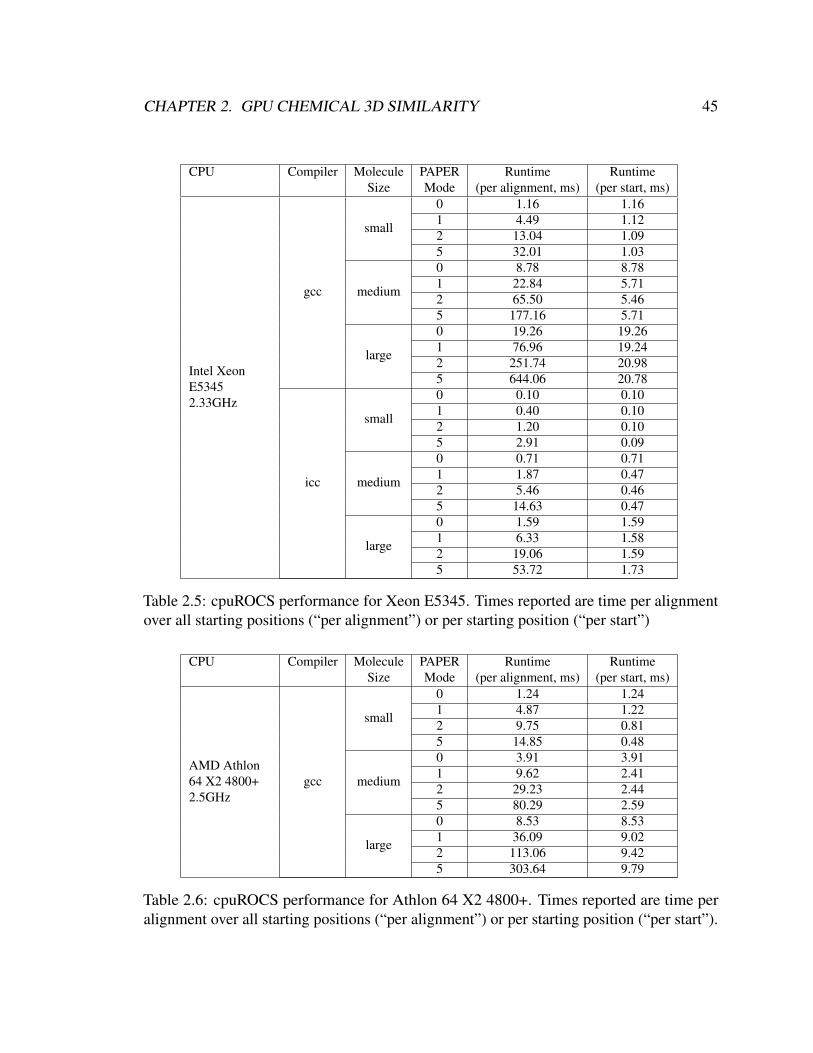
CHAPTER 2. GPU CHEMICAL 3D SIMILARITY 45
CPU Compiler Molecule PAPER Runtime RuntimeSize Mode (per alignment, ms) (per start, ms)
Intel XeonE53452.33GHz
gcc
small
0 1.16 1.161 4.49 1.122 13.04 1.095 32.01 1.03
medium
0 8.78 8.781 22.84 5.712 65.50 5.465 177.16 5.71
large
0 19.26 19.261 76.96 19.242 251.74 20.985 644.06 20.78
icc
small
0 0.10 0.101 0.40 0.102 1.20 0.105 2.91 0.09
medium
0 0.71 0.711 1.87 0.472 5.46 0.465 14.63 0.47
large
0 1.59 1.591 6.33 1.582 19.06 1.595 53.72 1.73
Table 2.5: cpuROCS performance for Xeon E5345. Times reported are time per alignmentover all starting positions (“per alignment”) or per starting position (“per start”)
CPU Compiler Molecule PAPER Runtime RuntimeSize Mode (per alignment, ms) (per start, ms)
AMD Athlon64 X2 4800+2.5GHz
gcc
small
0 1.24 1.241 4.87 1.222 9.75 0.815 14.85 0.48
medium
0 3.91 3.911 9.62 2.412 29.23 2.445 80.29 2.59
large
0 8.53 8.531 36.09 9.022 113.06 9.425 303.64 9.79
Table 2.6: cpuROCS performance for Athlon 64 X2 4800+. Times reported are time peralignment over all starting positions (“per alignment”) or per starting position (“per start”).

CHAPTER 2. GPU CHEMICAL 3D SIMILARITY 46
PAPER Mode Molecule Size GPU Batch Size Runtime Runtime(per alignment, ms) (per start, ms)
0 (1 startingorientation)
small
8600GT(32 SP)
1 0.76 0.7620 0.10 0.10
100 0.08 0.08500 0.08 0.08
8800GTX(128 SP)
1 0.63 0.6320 0.03 0.03
100 0.02 0.02500 0.02 0.02
GTX280(240 SP)
1 0.75 0.7520 0.04 0.04
100 0.01 0.01500 0.01 0.01
medium
8600GT(32 SP)
1 1.41 1.4120 0.21 0.21
100 0.17 0.17500 0.17 0.17
8800GTX(128 SP)
1 1.21 1.2120 0.06 0.06
100 0.05 0.05500 0.04 0.04
GTX280(240 SP)
1 1.58 1.5820 0.08 0.08
100 0.02 0.02500 0.02 0.02
large
8600GT(32 SP)
1 5.60 5.6020 0.88 0.88
100 0.76 0.76500 0.73 0.73
8800GTX(128 SP)
1 4.91 4.9120 0.26 0.26
100 0.20 0.20500 0.17 0.17
GTX280(240 SP)
1 5.38 5.3820 0.27 0.27
100 0.12 0.12500 0.07 0.07
Table 2.7: PAPER performance for initialization mode 0 on selected batch sizes. Timesreported are time per alignment over all starting positions (“per alignment”) or per startingposition (“per start”).

CHAPTER 2. GPU CHEMICAL 3D SIMILARITY 47
PAPER Mode Molecule Size GPU Batch Size Runtime Runtime(per alignment, ms) (per start, ms)
1 (4 startingorientations)
small
8600GT(32 SP)
1 21.25 5.3120 8.52 2.13
100 9.42 2.35500 10.22 2.55
8800GTX(128 SP)
1 18.73 4.6820 2.89 0.72
100 2.54 0.63500 2.46 0.62
GTX280(240 SP)
1 2.76 0.6920 0.15 0.04
100 0.11 0.03500 0.10 0.02
medium
8600GT(32 SP)
1 2.06 0.5220 0.96 0.24
100 0.97 0.24500 0.97 0.24
8800GTX(128 SP)
1 1.79 0.4520 0.27 0.07
100 0.23 0.06500 0.23 0.06
GTX280(240 SP)
1 5.75 1.4420 0.31 0.08
100 0.25 0.06500 0.22 0.05
large
8600GT(32 SP)
1 7.22 1.8020 3.66 0.92
100 3.65 0.91500 3.67 0.92
8800GTX(128 SP)
1 6.34 1.5820 0.98 0.25
100 0.86 0.22500 0.84 0.21
GTX280(240 SP)
1 6.48 1.6220 0.41 0.10
100 0.37 0.09500 0.33 0.08
Table 2.8: PAPER performance for initialization mode 1 on selected batch sizes. Timesreported are time per alignment over all starting positions (“per alignment”) or per startingposition (“per start”).

CHAPTER 2. GPU CHEMICAL 3D SIMILARITY 48
PAPER Mode Molecule Size GPU Batch Size Runtime Runtime(per alignment, ms) (per start, ms)
2 (12 startingorientations)
small
8600GT(32 SP)
1 23.26 1.9420 17.11 1.43
100 16.74 1.40500 16.67 1.39
8800GTX(128 SP)
1 18.74 1.5620 6.69 0.56
100 6.49 0.54500 6.38 0.53
GTX280(240 SP)
1 7.56 0.6320 0.80 0.07
100 0.79 0.07500 0.78 0.07
medium
8600GT(32 SP)
1 4.64 0.3920 4.00 0.33
100 3.95 0.33500 3.95 0.33
8800GTX(128 SP)
1 3.75 0.3120 1.33 0.11
100 1.27 0.11500 1.26 0.10
GTX280(240 SP)
1 8.07 0.6720 0.91 0.08
100 0.90 0.08500 0.90 0.07
large
8600GT(32 SP)
1 42.21 3.5220 27.75 2.31
100 27.69 2.31500 27.37 2.28
8800GTX(128 SP)
1 31.59 2.6320 11.41 0.95
100 10.85 0.90500 10.74 0.89
GTX280(240 SP)
1 17.94 1.5020 2.83 0.24
100 2.49 0.21500 2.42 0.20
Table 2.9: PAPER performance for initialization mode 2 on selected batch sizes. Timesreported are time per alignment over all starting positions (“per alignment”) or per startingposition (“per start”).
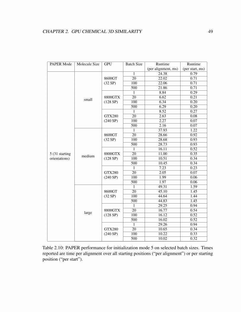
CHAPTER 2. GPU CHEMICAL 3D SIMILARITY 49
PAPER Mode Molecule Size GPU Batch Size Runtime Runtime(per alignment, ms) (per start, ms)
5 (31 startingorientations)
small
8600GT(32 SP)
1 24.38 0.7920 22.02 0.71
100 22.06 0.71500 21.86 0.71
8800GTX(128 SP)
1 8.84 0.2920 6.62 0.21
100 6.34 0.20500 6.29 0.20
GTX280(240 SP)
1 8.52 0.2720 2.63 0.08
100 2.27 0.07500 2.16 0.07
medium
8600GT(32 SP)
1 37.93 1.2220 28.66 0.92
100 28.68 0.93500 28.73 0.93
8800GTX(128 SP)
1 16.11 0.5220 11.00 0.35
100 10.51 0.34500 10.45 0.34
GTX280(240 SP)
1 7.23 0.2320 2.05 0.07
100 1.99 0.06500 1.97 0.06
large
8600GT(32 SP)
1 49.31 1.5920 45.10 1.45
100 44.64 1.44500 44.83 1.45
8800GTX(128 SP)
1 29.25 0.9420 16.77 0.54
100 16.12 0.52500 16.02 0.52
GTX280(240 SP)
1 29.26 0.9420 10.65 0.34
100 10.22 0.33500 10.02 0.32
Table 2.10: PAPER performance for initialization mode 5 on selected batch sizes. Timesreported are time per alignment over all starting positions (“per alignment”) or per startingposition (“per start”).

Chapter 3
GPU Acceleration of SMILES-based 2DChemical Similarity
Abstract
LINGOs are a holographic measure of chemical similarity based on text comparison of
SMILES strings. We present a new algorithm for calculating LINGO similarities amenable
to parallelization on SIMD architectures (such as GPUs and vector units of modern CPUs).
We show that it is nearly 3 times as fast as existing algorithms on a CPU, and over 80 times
faster than existing methods when run on a GPU.
This chapter has previously appeared in reference [42].
50

CHAPTER 3. GPU CHEMICAL 2D SIMILARITY 51
3.1 Introduction
The continuing exponential increase in computer power has made searches in chemical
databases of thousands to millions of compounds routine. A variety of techniques exist
for similarity search [64], ranging in computational complexity from 3-D superposition
methods [33, 58, 75] to simple substructure-fingerprint searches [16, 25]. The Lingo method
of Vidal, Thormann, and Pons [85] is a particularly simple algorithm that measures chemical
similarity by computing the similarity between the SMILES representations of two given
molecules. Despite its simplicity, LINGO has demonstrated accuracy comparable to path-
based substructural fingerprint methods [34]; its compelling advantages are speed and the
ready availability of appropriate SMILES representations for molecules.
While LINGO is one of the fastest similarity techniques in general usage, emerging
problems in cheminformatics necessitate dramatically faster methods for calculating similar-
ities. Freely available databases such as ZINC [45] (34 million molecules) and PubChem
(31 million molecules) are currently being used for a variety of cheminformatic analyses.
Exhaustive calculations on multi-million molecule databases such as these present a chal-
lenge to many commonly-used algorithms. Even more difficult are exhaustive databases
such as GDB-13 [8], which enumerates all 970 million molecules up to 13 heavy atoms
containing C, N, O, S, and Cl, according to a set of simple rules encoding chemical stability
and feasibility. Virtual combinatorial libraries can also present a challenge to conventional
algorithms, as even a 3 or 4 component combinatorial library can easily exceed a billion
molecules.
Scalability problems arise both from database size and the algorithms considered. The
largest current enumerated databases are nearly 1 billion (109) molecules in size [8]; future
libraries are likely to be larger. While search for a single query molecule can be done
in linear time, useful algorithms such as clustering chemical databases often run in time
quadratic in the size of the database or worse [15]. Consequently, as the size of both public
and corporate compound collections increases, faster similarity methods are required to
handle the increasing computational load.
The GPU revolution in computing offers a way to cope with these issues. Modern GPUs
(graphics processing units) are flexibly-programmable processors which offer theoretical
CHAPTER 3. GPU CHEMICAL 2D SIMILARITY 52
speedups over 30-fold relative to top-end conventional CPUs. GPUs have been applied, with
great effect, to related problems in computational chemistry, including molecular dynamics
[28, 81] and 3D similarity search [39]. Although GPUs often require algorithms to be
redesigned to achieve peak speedup, such changes also often benefit modern CPUs.
In this paper we present SIML (“Single-Instruction, Multiple-LINGO”), a new algorithm
(related to sparse matrix-matrix multiply) to calculate the LINGO similarity metric between
molecules, especially suited for efficient execution on GPUs and the vector units of current
CPUs. We describe a non-vectorized CPU version of our algorithm that is nearly 3 times as
fast as existing algorithms for calculating LINGOs and a GPU implementation that is over 80
times as fast as existing methods. Our code is available at https://simtk.org/home/
siml. We begin by explaining the LINGO similarity metric, continue with a description
of our algorithm, present performance benchmarks, and conclude with a discussion of
extensions of our work to generalizations of the considered LINGO similarities.
3.2 Methods
3.2.1 Overview of LINGO
The LINGO algorithm [85] models a molecule as a collection of substrings of a canonical
SMILES representation. Specifically, a SMILES string (after some simple transformations,
such as resetting all ring closure digits to zero) is fragmented into all its contiguous substrings
of length q, producing the set of “q-Lingos” for that molecule. The similarity between a pair
of molecules A and B is then defined by the following equation:
TA,B =1
`
∑i=1
(1− |NA,i −NB,i|
NA,i +NB,i
)(3.1)
In this equation, ` represents the number of Lingos present in either A or B, and Nx,i
represents the number of Lingos of type i present in molecule x. In this paper, we will
use the lowercase “Lingo” to refer to a substring of a SMILES string and the all-capitals
“LINGO” to refer either to the method, or the Tanimoto similarity resulting from the method.
Grant et al. have presented an efficient algorithm to calculate this Tanimoto value given

CHAPTER 3. GPU CHEMICAL 2D SIMILARITY 53
a pair of SMILES strings [34]. Their algorithm, given two SMILES strings of lengths m
and n, first constructs in Θ(m) time a finite state machine representation of one SMILES
string and all its valid Lingos. It then processes the second string through this FSM in Θ(n)
time, yielding a total runtime linear in the sum of the length of the two strings.
The use of the LINGO algorithm requires choosing a particular value of q, the SMILES
substring length. Values of q that are too small retain little structural information about
molecules; values that are too large induce too many distinct Lingos, making it increasingly
unlikely that a pair of molecules will have Lingos in common. Both Vidal et al. [85] and
Grant et al. [34] demonstrated that setting q = 4 (i.e., considering SMILES substrings of
length 4) had the best performance in a variety of cheminformatics applications.
3.2.2 Our Algorithm
The LINGO Tanimoto equation can be written in a simpler form using set notation. Specif-
ically, we treat a molecule as a multiset of q-Lingos; a multiset is a generalization of a
set that allows each element of a set to have multiplicity greater than 1. The union of two
multisets contains all elements present in either set, with multiplicity equal to the maximum
multiplicity of that element in either set. Similarly, the intersection of two multisets has only
those elements present in both sets, with multiplicity equal to the minimum multiplicity
in either set. In this model, the LINGO Tanimoto between a pair of molecules takes the
following simple form:
TA,B =|A ∩B||A ∪B|
(3.2)
Computer systems typically represent a character with 8 bits; thus, there is a one-to-one
correspondence between q-Lingos and 8q-bit integers. The optimality of q = 4 is fortuitous,
as 4-Lingos correspond to 32-bit integers, which map directly to the typical word length of
modern CPUs and GPUs (but see the conclusion for discussion of efficient implementations
where q 6= 4). This mapping means that current hardware can perform a comparison
between two 4-Lingos in one operation, rather than the 4 that would be needed for individual
characters. We thus represent each molecule as a multiset of 32-bit integers: a sorted vector
of 4-Lingos (represented as integers), and a parallel vector containing the multiplicity of

CHAPTER 3. GPU CHEMICAL 2D SIMILARITY 54
each Lingo.
This multiset intersection/union can also be interpreted as a modified vector Tanimoto
operating on sparse vectors A and B. In this interpretation, A and B are extremely-high
dimensional vectors, in which each coordinate specifies the number of Lingos present in
the molecule of a given type; the dimensionality is determined by the number of possible
Lingos. If each Lingo consists of four 8-bit characters, then the implicit dimensionality is
232; however, since most of these Lingos will not be present, the vector is highly sparse.
Consider the vector Tanimoto equation:
TAB =〈A,B〉
〈A,A〉+ 〈B,B〉 − 〈A,B〉(3.3)
If addition is kept as normal and multiplication of two numbers is replaced by taking the
minimum of the two it is trivial to prove that this modified vector Tanimoto calculates the
exact same quantity as the multiset definition given above (indeed, an equivalent expression,
motivated differently, is given by Grant et al. [34]). This interpretation (which uses the
same representation in memory as the multiset interpretation) has the advantage that the
set magnitudes 〈A,A〉 and 〈B,B〉 need not be calculated for every Tanimoto calculation;
only the intersection size 〈A,B〉 must be calculated each time. Indeed, the set magnitudes
are determined by the SMILES length ` and Lingo size q: 〈x, x〉 = `x − q + 1. This sparse
vector algorithm therefore saves the computation involved in calculating the set union in the
multiset algorithm.
Given a pair of molecules represented in the paired-array manner listed above, the
LINGO Tanimoto between them can be calculated in linear time using an algorithm similar
to merging sorted lists (Algorithm 1).
3.2.3 GPU implementation
The finite-state-machine algorithm of Grant et al. [34] is poorly adapted to execution on a
GPU or other SIMD processor because it requires either a large amount of branching or a
moderately-sized lookup table to implement FSM state transitions. While it is possible to
write branch-dense code for a GPU, such code typically performs poorly because different

CHAPTER 3. GPU CHEMICAL 2D SIMILARITY 55
Data: sorted lists a and b containing Lingos, sorted lists ac and bc containing Lingocounts, scalars `a and `b the lengths of lists a and b, and scalars ma =
∑ac and
mb =∑bc.
Result: LINGO Tanimoto between molecules a and bIndices into lists a/ac and b/bci = j = 0;Accumulator for magnitude of intersection between a andbisct = 0;while i < `a and j < `b do
if a[i] == b[j] thenisct += min(ac[i],bc[j]) ;i += 1;j += 1;
else if a[i] < b[j] theni += 1;
elsej += 1;
endendreturn (isct/ (ma +mb − isct))
Algorithm 1: Sparse-vector algorithm to calculate LINGO Tanimoto between twomolecules in sorted multiset representation

CHAPTER 3. GPU CHEMICAL 2D SIMILARITY 56
lanes in the vector unit must execute different code paths. The latter option, a large random-
access lookup table, falls prey to memory constraints. The GPU has only a very small
amount of low-latency “shared” memory with true random access on-chip (16KB on recent
NVIDIA GPUs). If the lookup table is larger than the available shared memory, then it must
be placed in off-chip “global” memory; however, good performance on GPUs requires that
global memory be accessed with spatial locality among threads. This behavior is unlikely
for a state-transition lookup table.
In contrast, our algorithm is well-suited for GPU implementation. In calculating a
similarity matrix, we assign each row of the matrix to a “thread block”, or virtual core,
on the GPU. Each thread block executes many threads, which calculate elements of the
row in parallel. Each thread block stores the multiset representation of its query molecule
(the molecule against which all column elements are compared) in shared memory to
minimize global memory accesses. Furthermore, we store database molecules (ones along
the columns of the similarity matrix) in column-major layout (such that the Lingos/counts
for each molecule lie in one column). This layout maximizes the spatial locality of memory
accesses by consecutive threads.
In architectures that require loads by adjacent lanes of a vector unit to be adjacent in
memory for high performance (e.g., Intel/AMD SSE, GPUs without texture caching), it
is possible to make a small modification to our algorithm to guarantee this characteristic.
We let j, the database molecule multiset index, be shared among all threads. We ensure
that each thread has advanced its i pointer (query multiset index) as far as possible before
j is incremented, so all threads always read from the same row in the transposed database
multiset matrix. In architectures with relaxed locality requirements (e.g., GPUs with 2-
D texture caching support), this row-synchronization can be removed, allowing higher
performance.

CHAPTER 3. GPU CHEMICAL 2D SIMILARITY 57
3.3 Results
3.3.1 Benchmarking Methodology
Our benchmark problem is the calculation of an all-vs-all LINGO Tanimoto matrix for a
set of compounds, which is a common first step for many algorithms in cheminformatics,
such as clustering. It is also relevant to doing multiple similarity searches, as the calculation
of each row of the matrix is equivalent to performing a database search against a different
query molecule.
For this particular problem it would be possible to halve the calculation by only evaluat-
ing the upper or lower triangle of the Tanimoto matrix, since using the same molecule set for
both query and database compounds induces a symmetric matrix. However, in the general
case different molecule sets may be used for the query and database sets (along the rows and
columns of the resulting matrix), resulting in an asymmetric matrix. We therefore bench-
marked the computation of the full Tanimoto matrix, rather than only the upper or lower
half, for greater generality. We benchmark the following Tanimoto calculation methods:
• OE: OpenEye implementation (OELingoSim) of the LINGO similarity method
• CPU: CPU implementation of our sparse vector algorithm using precalculated magni-
tudes and normal (row-major) database layout
• GPU: GPU implementation of our sparse vector algorithm using precalculated magni-
tudes, transposed (column-major) query layout, and 2-D texture fetching
All CPU performance testing was performed at Vertex on machine 1. GPU performance
testing was performed on two different machines at Stanford to assess code scaling:
• Machine 1: CPU: AMD Phenom II X4 920 (4 cores @ 2.8GHz)
• Machine 2: CPU: Intel Core 2 Quad Q6600 (4 cores @ 2.4GHz); GPU: NVIDIA
GeForce GTS 250 (128 SP @ 1.84 GHz)
• Machine 3: CPU: Intel Xeon E5420 (4 cores @ 2.5GHz); GPU: NVIDIA Tesla T10
(240 SP @ 1.44 GHz)

CHAPTER 3. GPU CHEMICAL 2D SIMILARITY 58
# molecules Average SMILES length (characters) Average # distinct Lingos4,096 35.17 29.318,192 35.41 29.5232,768 38.23 31.65
Table 3.1: Characteristics of SMILES sets from Maybridge used for benchmarking
The performance of our CPU code and the OpenEye LINGO implementation were
measured using a test code written in C++. We used OpenMP (a multi-platform standard
API for shared memory parallel programming) to parallelize both CPU methods to obtain
multi-core results. Our GPU implementation is written in Python, using the PyCUDA library
to access the GPU. Tanimoto calculations for both GPU and CPU codes were implemented
as requesting 240 rows of a Tanimoto matrix at a time to enable parallelization over rows.
All timing results were averaged over 6 runs.
Machines 1 and 2 used gcc 4.3.2; machine 3 used gcc 4.1.2. CPU code was compiled
with gcc -O2 -fopenmp. CUDA version 2.3 and NVIDIA driver version 190.29 were
used on both machines 2 and 3.
All SMILES strings used for testing were obtained from the ZINC database’s subset
of molecules from Maybridge [45]. Relevant statistics for the chosen benchmark sets are
shown in 3.1.
3.3.2 Performance
As a baseline performance benchmark, we evaluated the performance of the OpenEye
algorithm and our CPU multiset/sparse-vector algorithm on the construction of a similarity
matrix for a 4,096 molecule subset of the Maybridge database. The performance results on
Machine 1 are shown in 3.2. To evaluate GPU performance, we measured the time to con-
struct a similarity matrix on sets of 4,096, 8,192, and 32,768 molecules from Maybridge, on
machines 2 and 3. Measured times include the time to transfer sparse-vector-representation
molecules to the GPU as well as the time to transfer calculated Tanimotos back to the host.
GPU results are presented in 3.3.

CHAPTER 3. GPU CHEMICAL 2D SIMILARITY 59
Algorithm Time (ms) Throughput (kLINGOS/sec)OE 15060 1113
CPU 5460 3070OE parallel 3880 4320
CPU parallel 1420 11830Read SMILES + construct multisets 10.5 —
Table 3.2: Similarity matrix construction performance on CPU, 4,096 molecules, Machine 1(parallel = 4 cores)
Machine Number of molecules Time (ms) Throughput (kLINGOS/sec)2 4096 275 609002 8192 1026 654102 32768 16717 642303 4096 215 779003 8192 778 863003 32768 11637 92270
Table 3.3: Similarity matrix construction performance on GPU. Times include transfer ofmolecules to GPU and transfer of Tanimotos back to host. Note that total work performed isquadratic in the number of molecules.

CHAPTER 3. GPU CHEMICAL 2D SIMILARITY 60
3.4 Analysis
Our multiset/sparse-vector methods for calculating LINGO Tanimotos show significant
speedup relative to the existing best-in-class techniques for calculating LINGOs. The CPU
implementation shows a 2.75x speedup relative to the OpenEye method. This algorithm
incurs additional initialization overhead for each query string at the start of each row, whereas
in our method the preprocessing (constructing sorted-array multiset representations of the
SMILES strings) is performed at startup and not repeated. However, this startup cost is
amortized over the large calculation, amounting to less than 1% of the execution time even
for the parallel implementation of the CPU-based algorithm (last row, 3.2), and does not
significantly affect the achieved speedups. It is notable as well that our CPU implementation
is not vectorized to take advantage of the SSE capabilities on the tested Phenom II CPU.
As explained above, our algorithm is amenable to vectorization, and it may be possible to
obtain even larger speedups on the CPU.
Even larger speedups are achieved by moving the algorithm onto a GPU. On the 4K-
size problem, machine 2’s midrange GPU shows nearly 20x speedup relative to our CPU
sparse-vector algorithm, and nearly 55x relative to the OE algorithm. The throughput for
this midrange GPU falls off somewhat as the matrix size increases; this is likely due to
the increasing average size (29.3 Lingos at 4K to 31.6 Lingos at 32K) increasing the work
per Tanimoto calculation. In contrast, the throughput on the high-end GPU (machine 3)
continues to rise as the matrix size increases, indicating that even higher throughput may
be possible on larger problems. At the largest size we tested, the high-end Tesla T10 GPU
shows 30x speedup relative to our CPU method and nearly 83x speedup relative to the OE
technique.
Because they take advantage of the inherent parallelism in large-scale similarity calcu-
lations by parallelizing over row computations, our methods also scale very well to larger
hardware. Our CPU algorithm reaches 96.3% of linear speedup when parallelized over 4
cores with OpenMP. Our GPU code also shows excellent scaling; at the largest problem size,
we observe 97.9% of the expected throughput scaling, based on the increased number of
shaders and decreased clock speed on the Tesla T10 relative to the GeForce GTS 250.
While our algorithm is well suited to very-large-scale similarity calculations involving

CHAPTER 3. GPU CHEMICAL 2D SIMILARITY 61
the calculation of multiple rows of a Tanimoto matrix, it is not a good choice for small
calculations such as the scan of a single molecule against a SMILES database. Our algorithm
has a setup cost linear in the total number of molecules considered (query+database), whereas
the Grant et al. FSM-based algorithm only incurs cost for each query molecule. In the 1xN
(one query versus database of size N) case, the FSM algorithm thus has O(1) initialization
cost, whereas our sparse vector algorithm has O(N) initialization cost. For large (multiple-
row) calculations this setup cost is amortized because the same sparse-vector representations
of database molecules are reused at each row.
3.5 Conclusions
The growing size of chemical databases requires the development of faster methods of
chemical similarity comparison in order to implement database search, clustering, and
other cheminformatic algorithms. We have described a new algorithm for calculating the
LINGO similarity measure which is nearly 3x faster than the current best-in-class method.
This algorithm is well-suited to implementation on SIMD architectures like GPUs, and
demonstrates over 80-fold speedup versus OpenEye’s implementation of LINGO similarities
when run on a high-end GPU. Furthermore, this algorithm scales well to large hardware,
enabling high performance on new generations of CPU and GPU hardware. Implementations
of our algorithm are available at https://simtk.org/home/siml.
Our current implementations are focused on the LINGO algorithm with q = 4 (that is,
considering SMILES substrings of length 4) because they have been shown to be optimal for
typical similarity searches [34, 85]. However, in some cases, a different value of q may be
desirable (for example, extremely small molecules, in which there are few distinct Lingos,
or cases in which more specificity, and a larger Lingo size, is required). Our algorithm
is trivially extensible to q < 4; such Lingos correspond one-to-one with integers smaller
than 32 bits, so the remaining available bits can be replaced by zero and the algorithm
remains as previously described. It is also possible to extend the method to larger q. One
possibility is to extend the integer size — by using 64-bit integers, up to q = 8 can be
handled using the same method. Recent CPUs and upcoming GPUs natively support 64-bit
integers, potentially imposing little overhead (except doubled memory traffic) relative to the

CHAPTER 3. GPU CHEMICAL 2D SIMILARITY 62
use of 32-bit integers. Another option is to compress the Lingos. SMILES does not have a
full 256-character alphabet, and therefore does not require a full 8 bits per character. By
preprocessing strings the width of each character in a Lingo can be reduced. For example, if
only 64 characters are used in a set of molecules, each character will only require 6 bits, and
up to q = 5 can be supported still using 32-bit integers. Our algorithm is insensitive to these
issues, as it operates on integers of arbitrary width. While certain integer sizes may be faster
on given hardware, methods such as Lingo compression can be handled in preprocessing,
and do not affect the core multiset algorithm.
By providing nearly 2 orders of magnitude in speedup, our algorithm enables dramati-
cally larger calculations than previously possible. The use of GPU acceleration in particular
allows searches that previously required use of a cluster of hundreds of machines to be
performed on a user’s desktop; alternatively, lengthy searches can be performed in near-
realtime. We anticipate that these search capabilities will enable a new class of large-scale
cheminformatics applications for data fusion on very large databases.
Acknowledgments
The authors would like to thank Kim Branson for assistance with running CPU benchmarking
and Anthony Nicholls and Roger Sayle for helpful comments on the manuscript. ISH and
VSP acknowledge support from Simbios (NIH Roadmap GM072970).
Chapter 4
Optimization of GPU ChemicalSimilarity
Abstract
In this chapter we present the design and optimization of GPU implementations of two
popular chemical similarity techniques: Gaussian shape overlay (GSO) and LINGO. GSO
involves a data-parallel, arithmetically-intensive iterative numerical optimization; we use it
to examine issues of thread-parallelism, arithmetic optimization, and CPU-GPU transfer
overhead minimization. LINGO is a string similarity algorithm that, in its canonical
CPU implementation, is memory bandwidth- and branch-intensive and has limited data
parallelism. We present an algorithmic redesign allowing GPU implementation of such a
low arithmetic-intensity kernel, and discuss techniques for memory optimization that enable
large speedup. Source code for the programs described here is available online: PAPER (for
Gaussian shape overlay) can be downloaded at https://simtk.org/home/paper
under the GPL, and SIML (for LINGO) at https://simtk.org/home/siml under a
BSD license.
This chapter has previously appeared in reference [41].
63

CHAPTER 4. OPTIMIZATION OF GPU CHEMICAL SIMILARITY 64
4.1 Introduction, Problem Statement, and Context
Chemical informatics uses computational methods to analyze chemical datasets for applica-
tions that include search and classification of known chemicals, virtually screening digital
libraries of chemicals to find ones which may be active as potential drugs, and predicting and
optimizing the properties of existing active compounds. A common computational kernel
in cheminformatics is the evaluation of a similarity (using various models of similarity)
between a pair of chemicals. Such similarity algorithms are important tools in both academia
and industry.
A significant trend in chemical informatics is the increasing size of chemical databases.
Public databases listing known chemical matter exceed 30 million molecules in size, the
largest exhaustive libraries (listing all possible compounds under certain constraints) are
near 1 billion molecules, and virtual combinatorial libraries in use in industry can easily
reach the trillions of compounds. Unfortunately, similarity evaluations are often slow, at
or below 1000 evaluations/sec on a CPU. Adding to the problem, typical analyses in this
field (such as clustering) must execute a number of similarity evaluations that is supralinear
in the size of the database. The combination of rapidly growing chemical data sets and
computationally-expensive algorithms creates a need for new techniques.
The massive data and task parallelism present in large-scale chemical problems makes
GPU reimplementation an attractive acceleration method. In this article, we demonstrate
10-100× speedup in large-scale chemical similarity calculations, which allows the analysis
of dramatically larger datasets than previously possible. Search problems which formerly
would have required use of a cluster can now be efficiently performed on a single machine;
alternatively, formerly supercomputer-scale problems can be run on a small number of GPUs.
In particular, we show that two commonly used algorithms can be effectively parallelized on
the GPU: Gaussian shape overlay (GSO) [39], a 3-dimensional shape comparison technique,
and LINGO [42], a string comparison method.
4.1.1 Gaussian shape overlay: background
Gaussian shape overlay is an algorithm that measures the similarity of two molecules by
calculating the similarity of their shapes in 3-dimensional space. In this method, a molecule

CHAPTER 4. OPTIMIZATION OF GPU CHEMICAL SIMILARITY 65
is represented as a scalar field or function in 3-space, where the value of the function at
each point in space indicates whether or not the point is “inside” the molecule. Given a
set of functions ρAi(r) that represent the density functions for each atom of a molecule
(i.e., functions that are 1 inside the volume of an atom and 0 outside), the function for
an entire molecule can be defined using one of the formulas in equation 4.1. The first
computes interior points by taking the product of the complement of all atoms — defining
an “exterior point” as one which is not inside any atom. The latter method uses the principle
of inclusion-exclusion between sets to compute the same union of all atoms.
ρA (r) ≡ 1−N∏i=1
(1− ρAi (r))
ρA(r) ≡∑i
ρAi −∑i<j
ρAiρAj +∑i<j<k
ρAiρAjρAk −∑
i<j<k<l
ρAiρAjρAkρAl + · · ·(4.1)
Equation 4.1 is motivated by considering each atom to be a set of points, and constructing
the union of these sets. Defining atomic densities as indicator functions (one inside a given
radius around a point and zero outside) generates the “hard-sphere” model of molecular
shape. This model has several shortcomings (including nondifferentiability) that makes it
difficult to use in computations. Consequently, Grant and Pickup developed the Gaussian
model of molecular shape, in which each atom’s density function is defined not as a hard
sphere, but as an isotropic spherical Gaussian function:
ρAk(r) = pk exp(−αk||rk − r||2
)(4.2)
Such Gaussian functions are smooth and differentiable. Furthermore, simple closed-
form expressions for the volumes, volume gradients (with respect to position), and Hessians
of the product of an arbitrary number of such Gaussians are known [35]. This enables
the calculation of the similarity of two molecules by calculating the maximum overlap
possible between their shapes, maximized over all rigid-body transformations (translations
and rotations). Mathematically, GSO seeks to maximize equation 4.3 over all rigid body
transformations. In this integral, the functions ρA and ρB are the density fields for each
molecule and the integral is taken over all space.

CHAPTER 4. OPTIMIZATION OF GPU CHEMICAL SIMILARITY 66
∫drρAρB (4.3)
The computation is performed by numerical optimization to orient a pair of molecules
in their optimally-overlapping poses, and then computing the overlap volume (Figure 4.1)
[33]. The objective function in such a calculation is typically a truncated form of Equation
4.1, including only the single-overlap terms (Equation 4.4). Thus, both the objective and
gradient calculations are arithmetically-intensive and data-parallel, involving a double-loop
over the atoms of each molecule and an exponential evaluation inside the loop body. These
aspects make GPUs an attractive platform to implement GSO. In the first half of this chapter,
we describe PAPER, our open-source implementation of GSO on NVIDIA GPUs [39].
∫drρAρB ≈
∫dr
(∑i,j
ρAiρBj
)(4.4)
4.1.2 LINGO: background
Whereas GSO represents a molecule by its three-dimensional shape in space, the LINGO
algorithm of Vidal, Thormann, and Pons takes a much simpler, text-based approach [85].
LINGO is a 2-D similarity method: one that operates on molecules as graphs (with vertices
representing atoms and edges representing atomic bonds), ignoring their 3-dimensional
shape. Instead of operating directly on this molecular graph, LINGO processes a linear
representation of the graph called a SMILES string, which is constructed by a depth-first
traversal of the graph. The characters in the SMILES string represent various graph features,
such as atom types, bond orders, ring openings and closings, and branching. Given a
SMILES string, LINGO represents a molecule as the set of all overlapping q-character
substrings in the SMILES (known as “Lingos”, as opposed to “LINGO” for the algorithm as
a whole). q is typically set to 4 (i.e., Lingos have length 4), as this has been demonstrated
to have superior performance in several applications. Figure 4.2 presents an example of a
molecule and its SMILES representation, and its LINGO substrings for q = 4.
The similarities between a pair of molecules A and B is defined by the following equation,

CHAPTER 4. OPTIMIZATION OF GPU CHEMICAL SIMILARITY 67
(a) Reference molecule (b) Query molecule
(c) Calculated overlay
Figure 4.1: 3D shape overlay of molecules. The reference and query molecules are depictedas sticks (to visualize bond structure) embedded within their space-filling representation.GSO rotates the query molecule to maximize its volume overlap (blue spheres) with thevolume of the reference (red mesh).
O
methyl ethyl ketone
Molecule
CCC(=O)C
CCC(=O)CCC(=C(=O(=O)
SMILES Lingos
Figure 4.2: Chemical graph structure of a common solvent, its SMILES representation, andits constituent Lingos.

CHAPTER 4. OPTIMIZATION OF GPU CHEMICAL SIMILARITY 68
where Nx,i represents the number of Lingos of type i in molecule x:
TA,B =1
`
∑i=1
(1− |NA,i −NB,i|
NA,i +NB,i
)(4.5)
The canonical high-performance CPU implementation to rapidly evaluate this similarity
on a CPU was presented by Grant et al. [34]. This algorithm is optimized for the case in
which many SMILES strings must all be compared against one query. The Lingos of the
query string are inserted into a trie, a tree data structure allowing fast prefix search of strings.
This trie is then converted into a deterministic finite state automaton [3]; successive database
strings can then be efficiently processed through this DFA. This algorithm suffers from a
large amount of branching and poor memory locality in the simulation of the DFA, and
generally has poor data-parallelism within each LINGO calculation. It is thus relatively
unattractive for GPU implementation. In the latter half of this chapter, we discuss the
algorithmic transformations and memory optimizations that enable the high-speed GPU
implementation in SIML, our open-source package to calculate LINGO similarities on GPUs
[42].
4.2 Core Methods
Large-scale chemical informatics calculations involve the calculation of many similarities at
the same time, and so have a large amount of task parallelism; we exploit this structure in
both problems by calculating a large number of similarities at a time. The GSO problem in
particular is arithmetic-bound: its inner loop involves the calculation ofO(MN) exponential
functions (where M and N are the number of atoms in the molecules being compared), and
must be executed many times in a numerical optimization scheme (Equation 4.4). We make
use of SIMD data parallelism and hardware evaluation of exponentials to maximize the
arithmetic throughput of GSO on the GPU. LINGO, as implemented for high performance
on the CPU, uses a deterministic finite-state automaton algorithm that exhibits large branch
penalties and poor memory access locality on the GPU. We describe an algorithmic redesign
for LINGO that minimizes branch divergence and makes special use of GPU hardware
(texture caching) to maximize memory throughput.

CHAPTER 4. OPTIMIZATION OF GPU CHEMICAL SIMILARITY 69
4.3 Gaussian Shape Overlay: Parallelization and Arith-
metic Optimization
The GSO calculation is a numerical maximization of equation 4.4 over a seven-dimensional
space (3 translational coordinates and a 4-dimensional quaternion parameterization of a
rotation). In this section, we describe the design and optimization of PAPER, our GPU
implementation of GSO [39].
PAPER uses the BFGS algorithm [70], a “pseudo-second-order” method that uses
evaluations of the objective function and its first derivative (gradient), but no second-
derivative evaluations. Because BFGS is a local optimizer, and GSO is a global optimization
problem, we start each optimization from several initial points. The key computational steps
in this calculation are:
1. Repeatedly evaluate objective at test points along a search direction to find a “suffi-
ciently” improved point (line search)
2. Evaluate gradient at new point from line search
3. Update BFGS approximation to inverse Hessian matrix, and use this to calculate new
search direction
The primary consideration in software architecture for the GPU is partition of work:
what work should be done on the CPU vs the GPU, how work should be partitioned among
independent GPU cores (CUDA thread blocks or OpenCL work-groups), and how work
can be partitioned among threads or vector lanes in each core. PAPER makes use of the
extensive task-parallelism in chemical informatics to allocate work to GPU cores. Our target
applications focus on searches with hundreds to thousands of comparisons to be performed.
Because for each calculation we optimize from several (typically 4) starting points, GSO
yields a large number (# starting points × # molecules) of independent problems, each of
which can be assigned to an independent core (CUDA thread block or OpenCL work-group
). Partitioning work among GPU threads and between the CPU and GPU is more involved,
and is the focus of this section.

CHAPTER 4. OPTIMIZATION OF GPU CHEMICAL SIMILARITY 70
4.3.1 Evaluation of data-parallel objective function
Equation 4.4 describes the objective function that must be implemented in GSO. It is inher-
ently data-parallel, containing a double-loop over the M atoms of the reference molecule
and N atoms of the query molecule with an arithmetically-intensive loop body. This section
describes the parallelization of the objective calculation (which has the same structure as the
gradient), and presents several versions illustrating consecutive optimizations.
PAPER uses blocks of 64 threads to maximize the number of registers available to each
thread. While it can be advantageous in some cases to use larger thread blocks to hide
memory latency, in our application we typically have multiple thread blocks available on
each multiprocessor. Since scheduling is done on a per-warp basis, using many, smaller,
thread blocks is sufficient. In typical use cases, the number of terms to be calculated in
the objective is larger than the number of available threads: typical molecules are 20-40
atoms, so that normal calculations will have 400-1600 terms. To parallelize the problem, we
assign threads to calculate thread-block size “strips” of the interaction matrix consecutively,
until the entire set of interactions has been evaluated. Instead of using atomic operations to
accumulate the volume among threads, the function keeps an array in shared memory and
does a parallel reduction at the end to sum the final overlap volume. Figure 4.3 illustrates the
order of the computation, and Listing 4.1 provides code for a simple version of the objective
evaluation.
We perform an addressing calculation (lines 12-13) at each loop iteration so that each
thread evaluates the correct matrix element. Another strategy would be to disallow thread
blocks to span rows of the interaction matrix; however, this has the potential to leave many
threads idle, as there are usually more threads than the width of the matrix. Another option
would be the use of a two-dimensional thread block. However, because the number of atoms
varies by molecule in a batch, and because the number of atoms is not likely to be a multiple
of the GPU warp size, this also is likely to leave the GPU partially idle. Using the given loop
structure ensures that all threads do useful work as long as there are terms left to compute.
While the objective function in Listing 4.1 is effectively parallelized across all GPU
threads, several changes can be made to improve its performance. The first point of concern
is the addressing calculation. Because the number of atoms in either molecule is unlikely

CHAPTER 4. OPTIMIZATION OF GPU CHEMICAL SIMILARITY 71
1 /* Data: molecules ref and query2 * .natoms contains number of atoms in molecule3 * .xyz[i] contains coordinates for atom i4 * .a[i] is a scalar computed from the van der Waals radius of
atom i5 */6 float overlap(molecule ref, molecule query) {7 __shared__ float temp[]; // Has size equal to blockDim.x8 temp[threadIdx.x] = 0;9 for (int base = 0; base < ref.natoms * query.natoms;
10 base += blockDim.x) {11 int mycord = base + threadIdx.x;12 if (mycord < ref.natoms*query.natoms) {13 int ref_idx = mycord / query.natoms;14 int query_idx = mycord - ref_idx*query.natoms;15
16 float Rij2 = distance_squared(ref.xyz[ref_idx],17 query.xyz[query_idx]);18 float ref_a = ref.a[ref_idx], query_a = query.a[query_idx];19
20 float Kij = expf(-ref_a*query_a*Rij2/(ref_a+query_a));21 float Vij = Kij * 8 * powf(PI/(ref_a+query_a),1.5f);22 temp[threadIdx.x] += Vij;23 }24 }25 for (int stride = blockDim.x/2; stride > 0; stride >>=1) {26 __syncthreads();27 if (threadIdx.x < stride)28 temp[threadIdx.x] += temp[threadIdx.x+stride];29 }30 __syncthreads();31 return temp[0];32 }
Listing 4.1: First version of GSO objective function

CHAPTER 4. OPTIMIZATION OF GPU CHEMICAL SIMILARITY 72
0 5 10 150
5
10
Reference MoleculeAtom Index(ref_idx)
Query MoleculeAtom Index
(query_idx)
Figure 4.3: Thread parallelization scheme in PAPER. Depicted is the full matrix of in-teractions between a reference molecule of 11 atoms and a query molecule of 17 atoms.Thread blocks of 32 threads process consecutive 32-element strips of the matrix. Each colorrepresents one iteration of a thread block. Note that no more than a thread block-sized stripof matrix elements must be materialized at any time during the computation.
to be a power of two, it is necessary to use a division to calculate the row index for each
thread. However, integer division is a very expensive operation on current GPUs; when
performed in the inner loop, as in the original objective, it adds significant overhead. It is
possible to restructure the addressing such that the division is only performed once (Listing
4.2; non-addressing computations have been elided). Restructuring the calculation in this
way reduces the in-loop addressing overhead to two adds, a comparison, and two conditional
adds, which are much cheaper than the integer division. In the full PAPER implementation,
the objective is called multiple times per kernel invocation in the course of a line search;
thus, row per block and col per block are precalculated at the start of the kernel
invocation and stored in shared memory to amortize the cost of the division. Implementing
this change to the objective and gradient functions leads to a measured 13% speedup in total
optimization time.
With the integer division removed, the runtime becomes dominated by the evaluation of
Kij and Vij at lines 18-19 in Listing 4.1, which involves two divides and two transcen-
dental function evaluations — relatively expensive operations. The simplest optimization
to apply here is the use of CUDA intrinsic functions for the division and transcendentals.

CHAPTER 4. OPTIMIZATION OF GPU CHEMICAL SIMILARITY 73
1 float overlap(molecule ref, molecule query) {2 const int row_per_block = blockDim.x / query.natoms;3 const int col_per_block = blockDim.x - query.natoms*row_per_block;4 const int startrow = threadIdx.x / query.natoms;5 const int startcol = threadIdx.x - startrow * query.natoms;6 int ref_idx = startrow, query_idx = startcol;7 /* Shared memory setup goes here */8 while (ref_idx < ref.natoms) {9 /* Floating-point core computation goes here */
10
11 ref_idx += row_per_block;12 query_idx += col_per_block;13 if (query_idx >= query.natoms) {14 query_idx -= query.natoms;15 ref_idx++;16 }17 }18 /* Parallel reduction and return go here */19 }
Listing 4.2: Abbreviated GSO objective function with fast addressing
1 float exp_arg = __fdividef((-ref_a * query_a * Rij2),2 (ref_a + query_a));3 float Kij = __expf(exp_arg);4 float pow_arg = __fdividef(PI,(ref_a + query_a));5 float Vij = Kij * 8 * __powf(pow_arg,1.5f);
Listing 4.3: GSO core computation with CUDA intrinsics
CUDA intrinsics are low-level hardware operations that are often much faster than their
library versions, but at the cost of accuracy. In the GSO calculation, experimentation showed
that the reduced accuracy of intrinsic functions is not a problem. Listing 4.3 shows the use
of the expf, powf, and fdividef intrinsics to speed up the slow operations in the
objective core. Adding these three intrinsics more than doubles GSO performance with
respect to the previous version (Listing 4.2).
However, careful attention to instruction performance shows that this instruction stream
can be further improved. In particular, powf is expensive to evaluate, and it can be
replaced in this case by cheaper CUDA intrinsics: reciprocal and reciprocal square root.
As is often the case, this optimization produces results that are not numerically identical

CHAPTER 4. OPTIMIZATION OF GPU CHEMICAL SIMILARITY 74
1 const float PIRTPI = 5.56832799683f; // piˆ1.52 float sum = ref_a + query_a;3 float inv = 1.0f/sum; // CUDA intrinsic reciprocal4 float rsq = rsqrtf(sum); // CUDA intrinsic reciprocal square root5 float Kij = __expf(-ref_a * query_a * Rij2 * inv);6 float Vij = 8 * PIRTPI * rsq * inv * Kij;
Listing 4.4: GSO core computation with restructured CUDA intrinsics
Runtime per molecule SpeedupVersion (µs) vs originalOriginal 201 —
No-divide addressing 175 1.15×Intrinsic FP divide/transcendentals 84.9 2.37×
Restructured intrinsics 77.5 2.59×
Table 4.1: Effects of objective/gradient loop tuning on PAPER performance. Measured onGTX 480 with “large” molecule set at 2000 molecules/batch.
to the original; however, regression tested showed that the accuracy is sufficient for GSO.
The final computational core is provided as Listing 4.4 and is 10% faster than Listing 4.3.
Table 4.1 illustrates the performance gains from various tuning strategies on the overlap and
gradient kernels, as measured by their effect on the overall program runtime (not just the
overlap or gradient evaluation).
4.3.2 Kernel fusion and CPU/GPU balancing
It is common in multistage calculations such as GSO to have one or more steps which are
not efficiently parallelized on the GPU. In the case of GSO, while the line search/objective
evaluation and the gradient evaluation are very efficiently executed on the GPU (because
of high data parallelism and arithmetic intensity), the BFGS direction update is not well
parallelized. In PAPER, the BFGS update requires a large number of sequential low-
dimensional (7-D) vector operations and small (7x7) matrix operations. These operations
create a large amount of thread synchronization and many idle threads; it is thus not attractive
to compute them on the GPU. However, moving them to the CPU also imposes a cost. In the
case of the BFGS update, the coordinates, gradients, and objective values must be retrieved
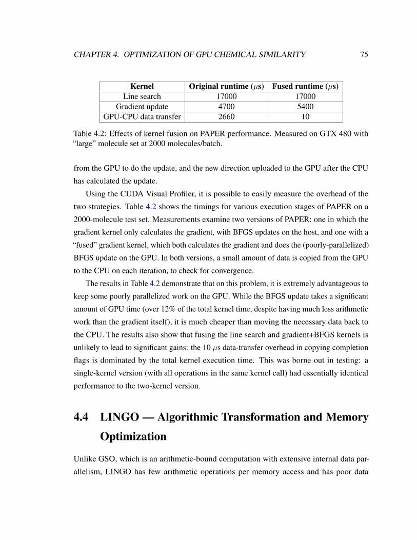
CHAPTER 4. OPTIMIZATION OF GPU CHEMICAL SIMILARITY 75
Kernel Original runtime (µs) Fused runtime (µs)Line search 17000 17000
Gradient update 4700 5400GPU-CPU data transfer 2660 10
Table 4.2: Effects of kernel fusion on PAPER performance. Measured on GTX 480 with“large” molecule set at 2000 molecules/batch.
from the GPU to do the update, and the new direction uploaded to the GPU after the CPU
has calculated the update.
Using the CUDA Visual Profiler, it is possible to easily measure the overhead of the
two strategies. Table 4.2 shows the timings for various execution stages of PAPER on a
2000-molecule test set. Measurements examine two versions of PAPER: one in which the
gradient kernel only calculates the gradient, with BFGS updates on the host, and one with a
“fused” gradient kernel, which both calculates the gradient and does the (poorly-parallelized)
BFGS update on the GPU. In both versions, a small amount of data is copied from the GPU
to the CPU on each iteration, to check for convergence.
The results in Table 4.2 demonstrate that on this problem, it is extremely advantageous to
keep some poorly parallelized work on the GPU. While the BFGS update takes a significant
amount of GPU time (over 12% of the total kernel time, despite having much less arithmetic
work than the gradient itself), it is much cheaper than moving the necessary data back to
the CPU. The results also show that fusing the line search and gradient+BFGS kernels is
unlikely to lead to significant gains: the 10 µs data-transfer overhead in copying completion
flags is dominated by the total kernel execution time. This was borne out in testing: a
single-kernel version (with all operations in the same kernel call) had essentially identical
performance to the two-kernel version.
4.4 LINGO — Algorithmic Transformation and Memory
Optimization
Unlike GSO, which is an arithmetic-bound computation with extensive internal data par-
allelism, LINGO has few arithmetic operations per memory access and has poor data

CHAPTER 4. OPTIMIZATION OF GPU CHEMICAL SIMILARITY 76
parallelism. Furthermore, while the GSO algorithm for the GPU is essentially a paral-
lelized version of the CPU GSO algorithm (BFGS), the canonical CPU algorithm for
high-performance LINGO is ill-suited to the GPU. This algorithm [34] compiles reference
strings into a deterministic finite state automaton, which is simulated for each query string.
To implement the DFA state transitions requires either significant amounts of branching,
or a moderately-sized, randomly-accessible lookup table (LUT); neither option is good
for GPUs. Branch-heavy code will pay a significant penalty in warp divergence. Worse,
none of the memory spaces in the CUDA memory model are well-suited to implement a
high-performance LUT of the type required: global memory requires aligned, coherent
access, texture memory requires spatial locality, constant memory requires that all threads in
a warp access the same element for high performance, and shared memory is limited in size.
Global, texture, and constant memory are inappropriate for a random-access LUT because
different threads are unlikely to use coherent accesses; shared memory is small and may not
be able to hold the LUT while maintaining reasonable SM occupancy (necessary to hide the
latency of streaming database Lingos in from global memory). In this section, we discuss
the design and optimization of SIML, our algorithm to calculate LINGOs efficiently on the
GPU [42].
Consequently, an algorithmic transformation is necessary to implement LINGO effi-
ciently on the GPU. The standard LINGO equation (Equation 4.5) can be recast into a
different form:
TA,B =|A ∩B||A ∪B|
=|A ∩B|
|A|+ |B| − |A ∩B|(4.6)
In this equation, each molecule (A or B) is represented as a multiset, a generalization
of a set in which each element can have cardinality greater than one; the multiset for a
molecule contains its Lingos and their counts. The cardinality of each element in a multiset
intersection is the minimum of its counts in either set (or maximum, for a multiset union).
SIML thus represents each molecule as a pair of integer vectors: one containing the Lingos in
sorted order, and one with corresponding counts. Here, the optimality of q = 4 is fortuitous,
as it allows us to trivially pack a 4-character Lingo into a 32-bit integer (each character is
8 bits). SIML also precalculates the cardinality of each set independently; thus, the only

CHAPTER 4. OPTIMIZATION OF GPU CHEMICAL SIMILARITY 77
1 /* Data: sorted lists A and B containing Lingos,2 * sorted lists A_c and B_c with Lingo counts,3 * scalars L_a and L_b the lengths of A/A_c and B/B_c,4 * scalars m_a = sum(A_c) and m_b = sum(B_c)5 */6 float siml(int* A, int* B, int* A_c, int* B_c,7 int L_a, int L_b, int m_a, int m_b) {8 int i = 0, j = 0;9 int intersection = 0;
10 while ( i < L_a && j < L_b) {11 if (A[i] == B[j] {12 intersection += min(A_c[i],B_c[j]);13 i++, j++;14 } else if (A[i] < B[j]) {15 i++;16 } else {17 j++;18 }19 }20 return ((float) intersection) / (m_a + m_b - intersection);21 }
Listing 4.5: SIML multiset algorithm for calculating LINGO similarities
Algorithm Runtime for 8K × 8K (ms) Throughput (LINGO × 103/sec)DFA 11875 5651
Multiset/SIML 19746 2888
Table 4.3: Multiset vs. DFA algorithm performance on CPU, measured by calculating an8,192 × 8,192 LINGO similarity matrix on a Core i7-920.
quantity needed to calculate the similarity between two SMILES string is the size of their
multiset intersection. This can be efficiently calculated using the algorithm in the following
listing, similar to merging sorted lists (Listing 4.5).
While the simple structure of the algorithm makes it attractive on the GPU, it is not
optimal for the CPU. Table 4.3 compares the performance of the SIML multiset algorithm on
the CPU against a DFA-based LINGO implementation. The DFA method has nearly twice
the throughput of the multiset method. This reflects a common theme in GPU programming:
algorithms optimal for the GPU may in fact represent de-optimization for the CPU.

CHAPTER 4. OPTIMIZATION OF GPU CHEMICAL SIMILARITY 78
4.4.1 SIML GPU implementation and memory tuning
Because of the poor data parallelism in any single LINGO similarity calculation, we use an
individual CUDA thread per similarity; each thread in a block calculates the similarity of
its query molecule against a common reference molecule for the entire block. While this
approach makes good use of task parallelism in large-scale LINGO calculations, simply
running Listing 4.5 per-thread on the GPU results in very poor performance. The first
optimization is to load the block’s reference molecule into shared memory, rather than
global memory. Since all threads access the same reference molecule, this significantly
reduces global memory traffic. However, this is sufficient only to reach approximate
performance parity with the CPU.
The key to performance in the SIML kernel is memory layout. If multisets are laid out
in “molecule-major” order (all elements for a single molecule stored contiguously, followed
by the next molecule, etc.), as would be appropriate for the CPU implementation of SIML,
consecutive GPU threads read from global memory with a stride equal to the length of the
largest multiset (Figure 4.4(a)). This stride is typically larger than the global memory request
size, so a separate read transaction must be dispatched for every thread. This becomes the
critical bottleneck: with molecule-major multiset layout, the CUDA Visual Profiler indicates
that the kernel’s arithmetic throughput is only 15% of peak on a GeForce GTS 250.
Transposing the multiset layout, such that all multisets’ first elements are contiguous,
followed by the second elements, and so on, nearly solves the problem (Figure 4.4(b)).
However, each thread maintains its own index into its query multiset (a row index in the
“Lingo-major” multiset-matrix); if these indices differ, then memory access will be uncoa-
lesced. One option is to have a shared row index among all threads: each thread increments
its query multiset pointer as far as possible, and then waits at a barrier ( syncthreads)
before the block moves on to the next multiset row. While this solution ensures that all
global loads are coalesced, it has a relatively high overhead in threads that must wait idle
at the barrier; it is able to achieve 80% of peak arithmetic throughput. The best option on
GPU hardware is to associate a 2-dimensional texture with the multiset matrix, and use
texture loads instead of uncached global loads. Because the texture cache is optimized for
spatial locality, it is able to absorb the overhead of the misalignment in row indices between

CHAPTER 4. OPTIMIZATION OF GPU CHEMICAL SIMILARITY 79
threads. The SIML kernel using a 2-D texture for global memory access is able to achieve
100% of peak single-issue arithmetic throughput (as measured by CUDA Visual Profiler),
demonstrating that careful optimization of memory layout and access method can turn a
problem traditionally considered to be memory-bound into one that is arithmetic-bound. An
implementation of this transposed, textured kernel is provided as Listing 4.6.
M0 L0
M1 L0
M2 L0
M3 L0
M0 L1
M1 L1
M2 L1
M3 L1
M0 L2
M1 L2
M2 L2
M3 L2
M0 L3
M1 L3
M2 L3
M3 L3
M0 L4
M1 L4
M2 L4
M3 L4
M0 L5
M1 L5
M2 L5
M3 L5
M0 L6
M1 L6
M2 L6
M3 L6
M0 L7
M1 L7
M2 L7
M3 L7
(a) Molecule-major layout for CPU. Each thread pro-ceeds rightwards from a different row, leading to strided,uncoalesced global reads on the GPU without caching.
M0 L0 M1 L0 M2 L0 M3 L0
M0 L1 M1 L1 M2 L1 M3 L1
M0 L2 M1 L2 M2 L2 M3 L2
M0 L3 M1 L3 M2 L3 M3 L3
M0 L4 M1 L4 M2 L4 M3 L4
M0 L5 M1 L5 M2 L5 M3 L5
M0 L6 M1 L6 M2 L6 M3 L6
M0 L7 M1 L7 M2 L7 M3 L7
(b) Lingo-major layout forGPU. Threads proceed down-wards in adjacent columns.Using a barrier on row index,or a 2D texture, ensures thatreads stay coalesced as thecalculation proceeds.
Figure 4.4: “Molecule-major” and “Lingo-major” layouts for storing the Lingos of multiplemolecules in memory. Red squares indicate the memory addresses read by consecutivethreads. “MX LY” indicates the Yth Lingo of the Xth molecule.
4.5 Final evaluation
Figure 4.5 compares the performance of the tuned PAPER implementation against OpenEye
ROCS, a commercial implementation of Gaussian shape overlay. ROCS supports various
“modes”, which represent different approximations to the GSO objective function. The
objective implemented in PAPER is equivalent to the “Exact” mode in ROCS. ROCS

CHAPTER 4. OPTIMIZATION OF GPU CHEMICAL SIMILARITY 80
1 /* Data:2 * sorted list A containing Lingos for reference molecule3 * sorted list A_c containing counts for reference molecule4 * textures B_tex and B_c_tex, pointing to Lingo-major5 * matrices of query Lingos and counts6 * scalars L_a and L_b the lengths of A/A_c and B/B_c7 * scalars m_a = sum(A_c) and m_b = sum(B_c)8 * scalar maxL_b the longest length of any query molecule9 * list (height of matrix pointed to by B_tex)
10 * scalar b_offset the column index in B_tex containing data11 * for the query molecule to be processed12 */13
14 texture<int,2> B_tex, B_c_tex;15
16 float siml_colmajor(int* A, int* A_c, int L_a, int m_a,17 int m_b, int L_b, int maxL_b, int b_offset) {18 int i=0, j=0, intersection=0;19 int Bj,B_cj;20
21 // Special-case the empty set22 if (m_a == 0 || m_b == 0) return 0.0f;23
24 while (j < maxL_b) {25 if (j < L_b) {26 // Use 2D texture to coalesce loads through cache27 Bj = tex2D(B_tex, b_offset, j);28 B_cj = tex2D(B_c_tex, b_offset, j);29
30 while ( i < L_a && a[i] < Bj) i++;31
32 // Now a[i] >= bj or i == L_a33 if (i < L_a && a[i] == Bj) {34 intersection += min(A_c[i], B_cj);35 i++;36 }37 // Now a[i] > b[j] or i == L_a38 }39 j++;40 // If texturing is not used, synchronize here to coalesce
loads41 }42 return intersection/((float)(m_a + m_b - intersection));43 }
Listing 4.6: Transposed SIML algorithm for LINGO using 2D texturing to coalesce readson the GPU
CHAPTER 4. OPTIMIZATION OF GPU CHEMICAL SIMILARITY 81
performance was measured on one core of an Intel Core i7-920; PAPER was run on an
NVIDIA GeForce GTX 480. Because the complexity of the GSO kernel varies by the size
of the molecules being compared, we present speedup plots for small (10 atoms), medium
(22 atoms), and large (44 atoms) molecules. The chosen “medium” size corresponds to the
average heavy atom (non-hydrogen) count in a popular chemical screening library.
Two trends are immediately obvious from the graph. First, PAPER requires a large
number of molecules to be optimized at the same time for effective speedup. This is typical
for GPU algorithms, especially those relying on task-parallelism. Because PAPER only
dispatches one optimization per thread block, and the GPU can run multiple thread blocks
per GPU core (streaming multiprocessor, or SM, in NVIDIA terminology), it is necessary
to dispatch many optimizations before the GPU is fully loaded. Performance continues to
improve past this lower bound (present around 25 optimizations in the plot) because CPU-
GPU copy overhead and kernel dispatch latency can be more effectively amortized with
larger batch sizes. The second trend is that the GPU is less effective for very small molecules,
which only achieve slightly more than 10x speedup, rather than the 90-100x possible on
larger molecules. The number of interaction terms is very small for such molecules, so
that kernel setup, kernel dispatch time, and idle threads come to dominate performance.
Ultimately, however, PAPER is able to demonstrate two orders of magnitude speedup on
problem sizes typical in our application domain.
Figure 4.6 illustrates the performance of SIML on three generations of NVIDIA GPU,
compared to the performance of a DFA-based LINGO implementation (contributed by
NextMove Software) running on one core of an Intel Core i7-920. The benchmark problem
for both data sets was the computation of an all-vs-all similarity matrix on 32,768 molecules.
As shown in Table 4.3, the multiset-based algorithm runs at about half the speed of the
DFA algorithm on a CPU. However, the multiset algorithm performs very well on a GPU.
SIML achieves over 11x greater throughput than the CPU DFA LINGO implementation on
a G92-architecture GeForce GTS 250, and over 23x higher throughput on a GF100-based
GeForce GTX 480.

CHAPTER 4. OPTIMIZATION OF GPU CHEMICAL SIMILARITY 82
0
20
40
60
80
100
120
1 10 100 1000
Spee
dup
fact
or v
ersu
s Ope
nEye
RO
CS (E
xact
mod
e)
(Cor
e i7
-920
)
Simultaneous molecules/optimization (GeForce GTX 480)
Small (10 atoms) Medium (22 atoms) Large (44 atoms)
Figure 4.5: PAPER performance versus OpenEye ROCS
11.5
15.2
23.2
0.0
5.0
10.0
15.0
20.0
25.0
GeForce GTS 250 (G92, 128 SP)
Tesla T10 (GT200, 240 SP)
GeForce GTX 480 (GF100, 480 SP) Sp
eedu
prela&veto
DFALINGOson
CPU
(Corei7‐920
)
Tested GPU (Architecture, Shader Count)
Figure 4.6: SIML performance versus DFA-based LINGOs

CHAPTER 4. OPTIMIZATION OF GPU CHEMICAL SIMILARITY 83
4.6 Future Directions
We are investigating possible optimizations to both PAPER and SIML. In the PAPER
objective/gradient computational core (Listing 4.4), a significant amount of time is spent
calculating functions of the reference and query radii that are invariant over the course of the
optimization. In particular, the reciprocal and reciprocal square root functions together are as
expensive as the following exponential evaluation. One possible option is to precalculate the
relevant functions of the radii (ref a * query a * inv and 8 * PIRTPI * rsq
* inv) and store them in lookup tables in shared memory. This approach has the potential
to significantly reduce the number of operations in the core computation, but at the cost of
higher memory usage.
The SIML kernel is extremely sensitive to the design of the memory subsystem of
the underlying hardware. The version presented has been optimized for the G80/G92 and
GT200 NVIDIA architectures, for which texture reads are the only cached reads from global
memory. However, the recent GF100 (Fermi) architecture features, in addition to the texture
cache, L1 and L2 caches for global memory. It is possible that tuning access methods (such
as using non-textured global memory reads) or block sizes (to better fit cache sizes) may
significantly affect performance. In general, because LINGO is a memory-sensitive kernel,
investigating cache tuning beyond the simple texturing done here is an interesting avenue
for future work.
4.7 Acknowledgments
We thank Roger Sayle of NextMove Software for his contribution of a DFA-based LINGO
implementation for benchmarking and comparison.

Chapter 5
SCISSORS: A Linear-AlgebraicalTechnique to Rapidly ApproximateChemical Similarities
Abstract
Algorithms for several emerging large-scale problems in cheminformatics have as their
rate-limiting step the evaluation of relatively slow chemical similarity measures, such as
structural similarity or 3-D shape comparison. In this article we present SCISSORS, a
linear-algebraical technique (related to multidimensional scaling and kernel principal com-
ponents analysis) to rapidly estimate chemical similarities for several popular measures.
We demonstrate that SCISSORS faithfully reflects its source similarity measures for both
Tanimoto calculation and rank-ordering. After an efficient pre-calculation step on a database,
SCISSORS affords several orders of magnitude of speedup in database screening. SCIS-
SORS furthermore provides an asymptotic speedup for large similarity matrix construction
problems, reducing the number of conventional slow similarity evaluations required from
quadratic to linear scaling.
This chapter has previously appeared in reference [40].
84

CHAPTER 5. SCISSORS: APPROXIMATE SIMILARITIES 85
5.1 Introduction
A fundamental problem in cheminformatics is the calculation of similarity between two given
molecules. As a consequence, a large variety of similarity techniques exists [64]. These
measures have as their underlying information content a variety of molecular properties,
including various encodings of molecular substructure [16, 25, 85], molecular volume
[33, 89], molecular surface similarity [46], and electrostatic similarity [61]. While many
of the more complicated techniques are able to uncover relevant chemical similarities not
found by simpler methods [59, 75], they are often computationally expensive to evaluate.
Many important algorithms in cheminformatics contain as a critical subroutine these
pairwise similarity comparisons. For example, database search against a single query
(without filters) amounts to the evaluation of a similarity measure once for each database
molecule. More complicated algorithms, such as those for clustering [15] or network
construction [84] may require the evaluation of a number of similarities quadratic in the size
of the database, rather than linear. Evaluation of similarities can be a bottleneck, limiting
performance as well as the size of problems that can be considered. While fingerprint-style
methods have been developed to approximate these similarity measures [38], they lack
rigorous justifications of their accuracy.
A significant continuing trend in cheminformatics is the increasing size of virtual
chemical databases. Public libraries listing known chemical matter, such as PubChem (31
million molecules) and ZINC [45] (34 million molecules), are routinely used in database
searches. Continuing advances in both computational power and storage space enable the
use of even larger exhaustive and combinatorial databases. GDB-13 [8] is an exhaustive
database enumerating all 970 million possible compounds composed of 13 or fewer heavy
atoms (C, N, O, S, and Cl) according to simple stability and synthesizability criteria. Virtual
combinatorial libraries can similarly reach or exceed the 109 molecule mark, even with as
few as three or four points of substitution. In the limit, it is believed that as many as 1060
molecules are potentially synthesizable [9]. The combination of rapidly growing chemical
libraries with computationally-difficult similarity metrics suggests a need for dramatically
faster methods of calculating chemical similarity.
In this article, we present SCISSORS (“SCISSORS Calculates Interpolated Shape

CHAPTER 5. SCISSORS: APPROXIMATE SIMILARITIES 86
Signatures Over ROCS Space”), a mathematical technique that allows extremely rapid
approximate evaluation of compound similarity for a variety of different similarity measures.
In one application of interest, the calculation of an all-pairs similarity matrix over a large
number of compounds, SCISSORS offers an asymptotic speedup in terms of the number of
similarity calculations required from quadratic to linear scaling. We begin with a mathe-
matical derivation of the SCISSORS algorithm and demonstrate its accuracy at Tanimoto
estimation and generalizability to various similarity measures. In the discussion, we present
links to a method from machine learning known as kernel principal components analysis,
and show how these links justify optimality properties for SCISSORS and offer interesting
insights into the nature of chemical shape space. Finally, we present a method by which
SCISSORS allows asymptotic speedup (in terms of number of slow similarity evaluations)
on the quadratic-scaling problem of similarity matrix construction.
5.2 Method
One commonality among otherwise diverse techniques to calculate chemical similarity is
that regardless of the underlying method, similarities are often returned as a Tanimoto score.
While Tanimotos are often treated simply as real-valued similarities in the range [0,1], they
have additional mathematical structure which can be profitably used; this is seen in the
definition of the Tanimoto TAB between vectors A and B:
TAB ≡〈A,B〉
〈A,A〉+ 〈B,B〉 − 〈A,B〉(5.1)
Equation 5.1 can be rearranged to obtain an expression for the inner product between
two vectors in terms of their Tanimoto:
〈A,B〉 =TAB
1 + TAB(〈A,A〉+ 〈B,B〉) (5.2)
Using this equation, the derivation of the SCISSORS method proceeds with two assump-
tions. We first assume that molecules can be represented as vectors in some (unspecified)
inner product space. Given this assumption and a similarity measure on two molecules
f and g, one can identify these molecules with vectors A and B in Equation 5.2. It then

CHAPTER 5. SCISSORS: APPROXIMATE SIMILARITIES 87
makes sense to ask for the inner product between the two molecules. Since the Tanimoto
between the two is known, we must somehow calculate the “magnitude” of each molecule
(the 〈A,A〉 terms).
In the absence of further information, a parsimonious decision is to arbitrarily set all
magnitudes equal to 1 (that is, 〈A,A〉 = 〈B,B〉 = 1); this is equivalent to assuming that all
molecules should lie on the surface of a hypersphere of arbitrary dimensionN . Alternatively,
for certain measures we have more information and can assign meaningful values to the
magnitude (see Discussion for an example). For the purpose of the derivation, we take the
magnitudes as given (either from parsimony or knowledge of the measure). This implies
that it is possible to calculate the inner product between two molecules given their pairwise
Tanimoto score.
We further assume that the inner product space in question is <N , the space of vectors
with N real-number coordinates. Under this assumption, it becomes meaningful to try to
map molecules to vectors in <N in such a way as to preserve their inner products. Given a
“basis” set of molecules B = B1, · · · , Bk, k ≥ N we require that similarities be computed
between all pairs in B. These similarities are then transformed to inner products (using a
method appropriate for the measure in question), and placed into a matrix G such that Gij
contains the inner product between molecules Bi and Bj (a matrix of this form is known
in the statistical literature as a “Gram matrix”). We wish to find a factorization of G of the
form G = MMT , where M is an NxN matrix containing the molecule vectors along its
rows.
Since the elements of G are constructed from molecular similarities, G is real and
symmetric, and therefore has a spectral decomposition into eigenvectors V and eigenvalues
(in diagonal matrix D). From this, the desired factorization follows by simple algebraic
manipulation:
G = MMT = V DV T
= V D12D
12V T
=(V D
12
)(V D
12
)TM = V D
12 (5.3)

CHAPTER 5. SCISSORS: APPROXIMATE SIMILARITIES 88
The method described in equation 5.3 is also used to derive vector coordinates from
inter-point distances in classical multidimensional scaling (MDS) [22]. It has several prop-
erties which make it an appealing choice relative to other matrix factorizations (such as the
Cholesky decomposition, which also finds matrix M such that G = MMT [31]). First, the
MDS reconstruction of molecule vectors in N dimensions is guaranteed to most closely
approximate the given inner products, in a least-squares sense. Furthermore, the reconstruc-
tion dimension can easily be chosen by sorting the eigenvalues in order of decreasing value,
and setting to zero all eigenvalues after the first K (for an K-dimensional reconstruction).
Our method is also very closely related to a technique known as kernel PCA [77, 78]; this
relationship has interesting consequences explored in the Discussion.
One mathematical detail skipped in the derivation of equation 5.3 relates to the square
root performed on the eigenvalues. If the measure described by the inner products in G is a
Euclidean metric, thenGwill be positive semi-definite (i.e., it will have only zero- or positive-
valued eigenvalues) [22], and the square root will exist. However, there is no guarantee
that a generic molecular similarity measure will be a Euclidean metric (and we show in
our results that several popular measures are not). Because of the optimality properties
of MDS, however, the impact that these negative eigenvalues have on the approximation
depends on their magnitude relative to the positive eigenvalues. If no negative eigenvalue has
magnitude within the top K, then it would not be used in the K-dimensional reconstruction,
and does not affect the solution. We demonstrate in our results that for many popular
measures, negative eigenvalues are of sufficiently small magnitude that they do not affect the
reconstruction, and that these non-Euclidean measures can therefore be well-approximated
by Euclidean inner products. Furthermore, in the following section we describe a correction
factor that can be added to the basic MDS formula to allow interpolation of coordinates
associated with negative eigenvalues.
5.2.1 Correction Factors
One drawback of our inference procedure is that the optimization procedure (Equation 5.3)
does not respect the vector magnitude assumptions made at the beginning in the first step. In
particular, given any molecule A in the basis set with square-magnitude 〈A,A〉 = x and its

CHAPTER 5. SCISSORS: APPROXIMATE SIMILARITIES 89
low-dimensional vector approximation A, the approximated square-magnitude⟨A, A
⟩will
always be smaller than x, because we have ignored the magnitude associated with higher
(less-significant) dimensions.
As will be shown in the Results, this loss of magnitude can cause problems with the
absolute accuracy of resulting Tanimoto values (though rank orderings are often preserved).
One possible strategy for solving this problem would be to replace Equation 5.3 with a
constrained optimization method; however, the simplicity and ubiquity of implementation
of a method based on the spectral decomposition suggest that a procedure to correct the
results of the eigenvector decomposition would be useful. Consequently, we choose not to
examine constrained optimization methods, although this may be an interesting direction for
future work.
A simple correction technique is to simply scale each result vector to force its magnitude
to 1. Our testing showed this to be ineffective (data not shown). However, one correction
technique, which we call the slack coordinate method, did improve accuracy and furthermore
allows us to represent non-Euclidean geometries.
Slack coordinate method
Without loss of generality, we consider only the case in which we wish to correct all
vector magnitudes to unity. Given real vectors A and B of arbitrary dimension n (i.e.,
A,B ∈ <n) with magnitude less than one, we construct vectors A and B of unity magnitude
by augmenting them with one additional “slack” coordinate, as follows:
A = [a0 a1 · · · an−1 an]T
B = [b0 b1 · · · bn−1 bn]T
||A|| = AT A = 1
an = ±
√√√√1−n−1∑i=0
a2i bn = ±
√√√√1−n−1∑i=0
b2i (5.4)
An interesting aspect of this correction is that the slack coordinate is incompletely
specified, as the sign is indeterminate. As in the scaling case, we can derive an analytic

CHAPTER 5. SCISSORS: APPROXIMATE SIMILARITIES 90
correction for the resulting Tanimoto. For convenience, we define variables k1 and k2,
corresponding to the numerator and denominator, respectively, of the uncorrected Tanimoto
equation:
TAB =
n−1∑i=0
aibi
n−1∑i=0
a2i +n−1∑i=0
b2i −n−1∑i=0
aibi
=k1k2
(5.5)
We can then define the corrected Tanimoto in terms of these variables, and simple
algebraic transformations allow us to express the correction as a function of the uncorrected
Tanimoto and the (uncorrected) magnitudes of A and B:
||A||2 =n−1∑i=0
a2i ||B||2 =n−1∑i=0
b2i
TAB =
∑ni=0 aibi∑n
i=0 a2i
∑ni=0 b
2i −
∑ni=0 aibi
TAB =k1 + anbn
k2 + a2n + b2n − anbn
TAB =k1 ±
√1− ||A||2
√1− ||B||2
(2− k1)∓√
1− ||A||2√
1− ||B||2
k1 =TAB (||A||2 + ||B||2)
(1 + TAB)
k3 = ±√
1− ||A||2√
1− ||B||2
k4 = k1 + k3
TAB =k4
2− k4(5.6)
Although the sign of the slack coordinate (±√
1− ||A||2 or±√
1− ||B||2 for molecules
A and B, respectively) is unspecified, the analytic correction term k3 is not directly dependent
on the particular signs of the slack coordinates. Rather, if A and B are real vectors, k3has sign determined by whether A and B have the same or opposite signs in their slack
coordinate. The case in which k3 is always negative (that is, all pairs of vectors A and B have

CHAPTER 5. SCISSORS: APPROXIMATE SIMILARITIES 91
opposite signs in their slack coordinates) turns out to be especially useful. However, this
case is not realizable if we restrict our vectors A and B to lie in <n+1. As a demonstration,
consider three vectors A, B, and C with slack coordinates an, bn, and cn. Without loss of
generality, let an be negative and bn be positive. For cn to always have opposite sign to any
molecule it was compared to, it would have to be positive when molecule C is compared
with molecule A and negative when compared to B; this is a contradiction.
Although this style of correction term cannot be implemented with real vectors, by
generalizing the vector space, this result is easily understood. The case in which every pair
of vectors is associated with a negative correction term k3 corresponds to vectors lying in
<n ×=, where the slack coordinate is always positive in sign and purely imaginary (e.g.,
in equation 5.4, let an = i√
1−∑n−1
i=0 a2i , with i =
√−1). Strictly, this interpretation
requires that equation 5.4 be modified so that the Hermitian transpose is used, but does not
affect the rest of the derivation. The geometry implied by this vector space is known as
pseudo-Euclidean, in contrast with the Euclidean geometry of <n+1, and has the capability
to represent curved spaces. In particular, imaginary coordinates of this form can be used
to represent the curved dimensions induced by negative eigenvalues in the Gram matrix
[68]. The slack coordinate correction, by generalizing from real to complex vectors, allows
approximation of non-Euclidean distance measures.
5.2.2 Fast approximation of new vectors
The above procedure for deriving molecule vectors requires computation of O(k2) molecular
similarities. It therefore does not scale to computing vectors over large libraries of millions
of compounds. However, given a fixed “basis” set of molecules, it is possible to approximate
vectors for new molecules in a fixed amount of time for each new molecule by least-squares.
Specifically, given a “library” molecule (that is, one not originally in the basis set) Li and the
matrix M of basis vectors, a vector for Li can be constructed by the following procedure:
1. Compute similarities between Li and all basis molecules Bj
2. Transform similarities to inner products Gij
3. Store inner products in a vector T = [Gi1, Gi2, · · · , Gik]T

CHAPTER 5. SCISSORS: APPROXIMATE SIMILARITIES 92
4. Solve equation M~x = T by linear least squares
The resulting vector ~x contains the vector that best approximates the given inner products,
in a least-squares sense, and therefore is the molecule vector for molecule Li. This procedure
allows the approximation of vectors for a large library of molecules in time linear in the
size of the library. It is, furthermore, embarrassingly parallel once the basis set has been
computed, making it a computationally attractive method for operation on large libraries.
5.3 Results
Full details of the testing methods used in this work, including exact molecule counts,
software versions used, and software settings, are included in the Appendix.
5.3.1 Similarity Measures
To demonstrate the generality of the SCISSORS technique, we have tested it against similar-
ity measures of various types, as implemented in the OpenEye Scientific Software oechem,
oeshape, and oeet toolkits1. Representing substructure-fingerprint-based methods is LINGO,
a similarity measure which counts the number of substrings in common between the SMILES
representation of a pair of molecules [85]. ROCS [75], a 3D shape comparison method which
finds the maximal volume overlap between Gaussian representations of molecule shape,
represents 3D shape methods. A variation on shape-based ROCS, known as the ROCS Color
Tanimoto, uses a similar volume overlap optimization on virtual “color” atoms representing
chemical functionalities. We use this color ROCS to demonstrate the generalizability of
SCISSORS to 3D methods that include distinct atom types, not all of which interact with
one another. Finally, ZAP [59], a Poisson-Boltzmann solver which calculates and compares
electrostatic fields around molecules, represents electrostatic similarity methods.
1OpenEye Scientific Software, Santa Fe, NM

CHAPTER 5. SCISSORS: APPROXIMATE SIMILARITIES 93
5.3.2 Molecules Tested
We draw molecules for testing from a diverse set of collections of drug- and drug-like
molecules. Most of our tests are performed on a 57,253 molecule database, hereafter named
“Maybridge+BBP” constructed from the union of the Maybridge Screening Collection
and a blood-brain barrier penetration dataset [54]. For Maybridge+BBP, 3-D conformers
were generated using OpenEye’s OMEGA software. When calculating Tanimotos using
ROCS, multi-conformer (200 conformer maximum) fit molecules were aligned against
single-conformer references, and the maximum Tanimoto over any pair of conformations
for the molecule pair was used. Detailed configuration parameters passed to ROCS and
OMEGA are included in the Appendix.
In the test for generalizability of SCISSORS, we used the 1,665 molecules tested in
PubChem Assay #677, an assay for novel allosteric modulators of the M1 muscarinic
receptor. To test the sensitivity of the SCISSORS technique against the source of molecules
for the basis set, we draw basis molecules from the Maybridge+BBP set and also from the
Asinex Gold Collection and the Maybridge Fragment Library, commercial libraries used for
compound and fragment screening. Finally, the virtual screening test draws its molecules
from the Directory of Useful Decoys, version 2 [44], a computational drug-discovery data
set specifically designed to confound methods based on common physical parameters, such
as molecular weight and cLogP. For all 3-D similarity measures other than the 57,253
molecule Maybridge+BBP set, molecules were assigned single conformers by OpenEye’s
OMEGA software. Charges for all molecules were assigned using the AM1-BCC charge
model implemented in OpenEye’s oequacpac toolkit.
Differences in setup (i.e., multi-conformer vs single-conformer) between datasets are
due to the fact that we made use of existing databases already in use for other drug discovery
projects. These differences are not significant to the content of the paper. Insofar as the goal
of SCISSORS is to reproduce the results of existing similarity measures, we demonstrate
comparable performance to the source similarity measure regardless of how the molecules
were prepared for the source measures.

CHAPTER 5. SCISSORS: APPROXIMATE SIMILARITIES 94
5.3.3 Basis size and dimensionality
To evaluate SCISSORS’ ability to approximate molecular similarities on data sets of varying
size, we used SCISSORS to approximate the ROCS shape Tanimoto for test sets of 19,000
and 50,000 molecules drawn at random from Maybridge+BBP. This was performed multiple
times over a large number of basis sizes and dimensionalities (in all cases, the 19,000 or
50,000 library molecules were disjoint from the basis molecules). Tanimotos were computed
using multi-conformer query molecules matched against single-conformer references; the
Tanimoto of the best-matching query conformer against the reference was used as the
Tanimoto for the molecule pair. Detailed settings for ROCS are provided in the Appendix.
As a measure of performance, we calculated the RMS deviation between the SCISSORS
Tanimoto and the ROCS Tanimoto over all pairings of these 19,000 molecules (5.1; 19,000 x
19,000 = 361 million Tanimotos) or 50,000 molecules (5.2; 50,000 x 50,000 = 2,500 million
Tanimotos).
Two trends are evident from the data. First, the error in the SCISSORS approximation of
the shape Tanimoto falls rapidly at first with the addition of more dimensions, and then levels
off around 75-100 dimensions. Most of the error falloff occurs in the first few dimensions,
with gains beyond 30 dimensions coming much more slowly. A similar trend also appears
for basis size — a large error is present for small basis sizes (especially in high-dimensional
approximations), as a consequence of overfitting the vector model, but this falls off rapidly as
the basis size increases. This result is stable even as we scale to a data set more than double
the size. The test set comprising 50,000 molecules required neither more eigenvectors nor
a larger basis set to achieve RMS error comparable to that found on the 19,000 molecule
test set. Ultimately, SCISSORS is able to approximate the ROCS shape Tanimoto to within
approximately 0.08 RMS error around 75-100 dimensions and a basis size of 500-1000, for
both the 19,000- and 50,000-molecule test sets.
5.3.4 Basis selection strategies
To test the sensitivity of the SCISSORS technique to how the basis set is chosen, we
compared randomly-chosen basis sets with basis sets chosen such that basis molecules
corresponded to “representative” shapes in the dataset. To choose representative molecules,
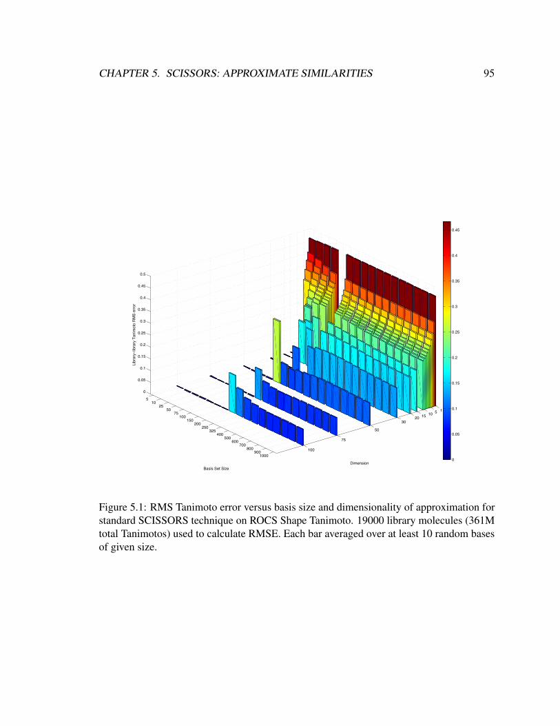
CHAPTER 5. SCISSORS: APPROXIMATE SIMILARITIES 95
510
2550
75100
150200
250325
400500
600700
800900
1000
1510152030
50
75
100
0
0.05
0.1
0.15
0.2
0.25
0.3
0.35
0.4
0.45
0.5
DimensionBasis Set Size
Libr
ary−
libra
ry T
anim
oto
RM
S er
ror
0
0.05
0.1
0.15
0.2
0.25
0.3
0.35
0.4
0.45
Figure 5.1: RMS Tanimoto error versus basis size and dimensionality of approximation forstandard SCISSORS technique on ROCS Shape Tanimoto. 19000 library molecules (361Mtotal Tanimotos) used to calculate RMSE. Each bar averaged over at least 10 random basesof given size.

CHAPTER 5. SCISSORS: APPROXIMATE SIMILARITIES 96
510
2550
75100
150200
250325
400500
600700
800900
1000
1510152030
50
75
100
0
0.05
0.1
0.15
0.2
0.25
0.3
0.35
0.4
0.45
0.5
DimensionBasis Set Size
Libr
ary−
libra
ry T
anim
oto
RM
S er
ror
0
0.05
0.1
0.15
0.2
0.25
0.3
0.35
0.4
0.45
Figure 5.2: RMS Tanimoto error versus basis size and dimensionality of approximation forstandard SCISSORS technique on ROCS Shape Tanimoto. 50000 library molecules (2500Mtotal Tanimotos) used to calculate RMSE. Each bar averaged over at least 10 random basesof given size.

CHAPTER 5. SCISSORS: APPROXIMATE SIMILARITIES 97
we clustered the Maybridge set using the dbclus algorithm [15] at several Tanimoto cutoff
values; the cluster centers chosen were used as the representative shapes. For each measured
basis size N, we ran SCISSORS in 75 dimensions using a basis consisting of N randomly-
chosen molecules, or the N cluster centers with largest number of neighbors (ties broken at
random). The resulting library RMS errors are plotted in 5.3.
For any basis set larger than 200 molecules, it was possible to find a SCISSORS
approximation with lower error than that resulting from the random basis; however, in
all cases such error reduction was extremely small: on the order of 0.005 Tanimoto units.
Interestingly, the optimal clustering Tanimoto value differed by basis size. The optimal
Tanimoto (that is, the cluster set with lowest RMS error) increased with increasing basis
size, suggesting that as more basis molecules are added, it is somewhat advantageous to
select tighter clusters as basis elements.
Random 0.65(261)
0.70(572)
0.75(1201)
0.80(2416)
0.85(4537)
0.90(7905)
0.95(12926)
Design Tanimoto for clustering(Number of cluster centers found in clustering)
0.070
0.075
0.080
0.085
0.090
0.095
0.100
Libra
ry-L
ibra
ry T
anim
oto
RM
S E
rror
(36
1M
Pair
s)
#Basis = 200#Basis = 250#Basis = 325#Basis = 500
Figure 5.3: RMS Tanimoto errors for SCISSORS approximations to ROCS shape Tanimotoconstructed from randomly-selected basis sets and basis sets chosen by molecule clustering.All Tanimotos evaluated over 361M molecule pairs.
5.3.5 Corrected Tanimotos
In 5.4 we examine the effect of the slack coordinate correction term introduced earlier.
Because the purpose of the correction term is to account for eigenspectrum density truncated
in a low-dimensional approximation, we examine two cases, 10 and 75 dimensional approxi-
mations. 5.4 is a density plot of SCISSORS standard and corrected Tanimotos versus ROCS
Tanimotos using the 19,000 molecule test subset of Maybridge+BBP also used in 5.1. In

CHAPTER 5. SCISSORS: APPROXIMATE SIMILARITIES 98
5.4, density contours that are symmetric about Y = X indicate that the plotted Tanimoto
values have an unbiased or independent error with respect to the original Tanimoto value,
which aids in the preservation of rank ordering.
As expected from the earlier results, in 75 dimensions, the standard SCISSORS Tanimoto
values are tightly clustered along the Y = X line, and the contours of the density plot
continue to be aligned along this Y = X axis even out to low densities, indicating an overall
preservation of rank-ordering. In contrast, in 10 dimensions, the SCISSORS Tanimotos,
as expected, almost always overestimate the true Tanimoto. Furthermore, the contours are
no longer ellipses symmetric about Y = X (or a parallel line), which indicates poorer
rank-ordering performance.
As expected, the slack coordinate correction leaves the high-dimensional case largely
unaffected, with the major exception of a large group of errors at ROCS Tanimoto = 1.0.
These are caused by self-comparisons — the slack coordinate method does not respect
the constraint that the Tanimoto of a vector against itself ought to be 1. However, in the
low-dimensional case, the slack correction makes a significant difference. Leaving aside
the known artifact at ROCS Tanimoto = 1.0, the overall shape of the density contours is
shifted below the diagonal, but is symmetric. This indicates that with the exception of
a constant shift, the slack-corrected values are much more accurate than the uncorrected
low-dimensional values.
5.3.6 Virtual screening
To illustrate the utility of SCISSORS-derived Tanimoto values in virtual screening, we
used SCISSORS on the ROCS shape Tanimoto to do a virtual screen on the Directory
of Useful Decoys (DUD) test set. DUD is a collection of “systems” consisting of target
proteins and associated small molecules. For each system, a certain number of molecules
known to bind the target are designated as “ligands”; the rest of the molecules (36 times the
number of ligands) are “decoys” with similar physical properties believed to not bind the
target. We used a previously-published protocol [39] to evaluate performance and statistical
significance; for clarity, we summarize the protocol below.
For each protein system in DUD, we used ROCS and SCISSORS (with three different
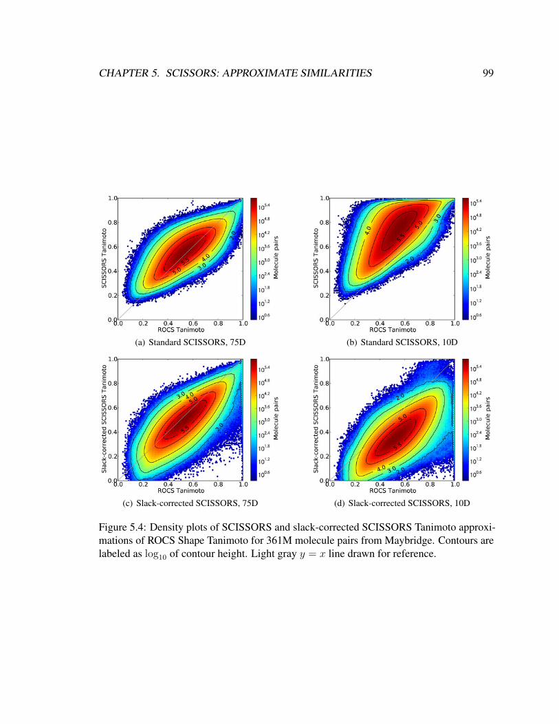
CHAPTER 5. SCISSORS: APPROXIMATE SIMILARITIES 99
(a) Standard SCISSORS, 75D (b) Standard SCISSORS, 10D
(c) Slack-corrected SCISSORS, 75D (d) Slack-corrected SCISSORS, 10D
Figure 5.4: Density plots of SCISSORS and slack-corrected SCISSORS Tanimoto approxi-mations of ROCS Shape Tanimoto for 361M molecule pairs from Maybridge. Contours arelabeled as log10 of contour height. Light gray y = x line drawn for reference.

CHAPTER 5. SCISSORS: APPROXIMATE SIMILARITIES 100
basis sets) to calculate the Tanimoto of every ligand molecule against every other molecule in
the system. For each ligand molecule, we ranked all other molecules in order of decreasing
Tanimoto similarity, modeling a screening experiment in which given one active compound,
one wishes to find other actives in a pool of inactive molecules. All molecules used were
single-conformer; settings for ROCS are given in the Appendix. All SCISSORS Tanimoto
values were computed in 10 dimensions as uncorrected SCISSORS Tanimotos. Basis sets
were drawn from the Maybridge Screening Collection, the Asinex Screening Collection,
and the Maybridge Fragment Library to illustrate the effects of different basis choices on
performance.
The ROC AUC for this ranking was calculated according to the method in Clark [20].
Ligand molecules were considered true positives; false positives were any decoys ranked
higher than a true ligand. A bootstrapping procedure [39] was used to estimate the 68%
and 95% confidence intervals on the calculated AUC values. These AUCs and confidence
intervals are illustrated in 5.5.
For almost all systems, the performance of the different SCISSORS basis sets are
statistically indistinguishable from each other and from that of the original ROCS Tanimoto.
In particular, the Maybridge and Asinex basis sets, which are drawn from different libraries
but which likely have overall similar characteristics (as both are screening libraries) perform
almost identically. The Maybridge Fragment basis is an outlier on several systems; it is
likely that this is because these molecules are significantly smaller (in volume/mass) than the
druglike molecules in DUD, indicating that at least rudimentary physical property matching
is a prudent step in the use of SCISSORS. It is interesting, however, that there were so
few outliers using the fragment basis set, as similarity measures often fail when comparing
fragments to elaborated molecules; we have not explored the reasons for this performance
in detail.
5.3.7 Similarity measure generalizability
To assess the generalizability of SCISSORS to chemical similarity measures other than the
ROCS shape Tanimoto, we evaluated the performance of SCISSORS on four similarity
measures: ROCS shape, ROCS color, LINGO, and ZAP’s ET, or electrostatic Tanimoto.

CHAPTER 5. SCISSORS: APPROXIMATE SIMILARITIES 101
Figure 5.5: ROC AUC values on each system of the DUD test set. Reported are themean AUC, averaged over each ligand in the system (line), the 68% confidence intervalon the AUC (box), and the 95% confidence interval on the AUC (whiskers). Within eachsystem, results are reported for ROCS (G, gray) and SCISSORS using basis sets from theMaybridge Screening Collection (M, red), the Asinex Screening Collection (A, orange), andthe Maybridge Fragment Library (F, blue). All SCISSORS approximations were done in10 dimensions; Maybridge and Asinex sets used a 500-molecule basis set; the MaybridgeFragment set was 473 molecules, the size of the entire library.

CHAPTER 5. SCISSORS: APPROXIMATE SIMILARITIES 102
All Tanimotos were originally evaluated on a collection of 1,665 small molecules from a
screen for allosteric modulators of the M1 muscarinic receptor; for SCISSORS, both basis
and library molecules were drawn from this same pool. All tests were conducted with 1,000
library molecules, with RMS errors evaluated over an all-pairs (1,000 x 1,000 = 1 million
Tanimotos) similarity comparison. For the electrostatic Tanimoto, molecules were first
overlaid using ROCS before electrostatic field calculation.
5.6 plots the SCISSORS Tanimoto RMS error for each similarity measure in the large
basis (600 molecules) limit as a function of dimensionality. Three trends are particularly
notable. First, on this dataset, all the similarity measures show non-monotonic error be-
havior as the number of dimensions increases, most likely reflecting eventual overfitting
(an insufficient number of basis molecules for further dimensions). Second, SCISSORS
generalizes well to approximating both the ROCS color and the LINGO Tanimotos, with
RMS errors under 0.1 in both cases. Finally, ZAP’s electrostatic Tanimoto appears to be
inapproximable by the SCISSORS method.
5.7 explores why only certain measures are approximable by SCISSORS. Each subplot
plots the value of the top 300 eigenvalues from a basis set of size 1000 computed for each
of the four similarity measures, on a log scale. For all three well-approximated measures,
the magnitude of the 100th eigenvalue has fallen off more than 2 log units relative to
the first (largest) one, indicating that high dimensions rapidly become less important to
the approximation. In contrast, the ET Tanimoto’s eigenspectrum falls off much more
slowly — even after 300 dimensions, it has not fallen 2 log units. It is this characteristic
of the eigenspectrum (insufficiently rapid falloff) that makes a low-dimensional linear
approximation to the ET Tanimoto impossible.
5.3.8 Tanimoto Computation Speed
The precalculation step of SCISSORS is extremely efficient compared to the evaluation of the
source similarity measure. We benchmarked the precalculation step for calculating molecule
vectors on a 20,480 molecule subset of Maybridge+BBP, using a 500 molecule basis set
drawn from the same database. Timings for each phase of SCISSORS precalculation on one
core of a 3GHz Intel Xeon-based (Core 2-architecture) Mac Pro are presented in 5.1 (further
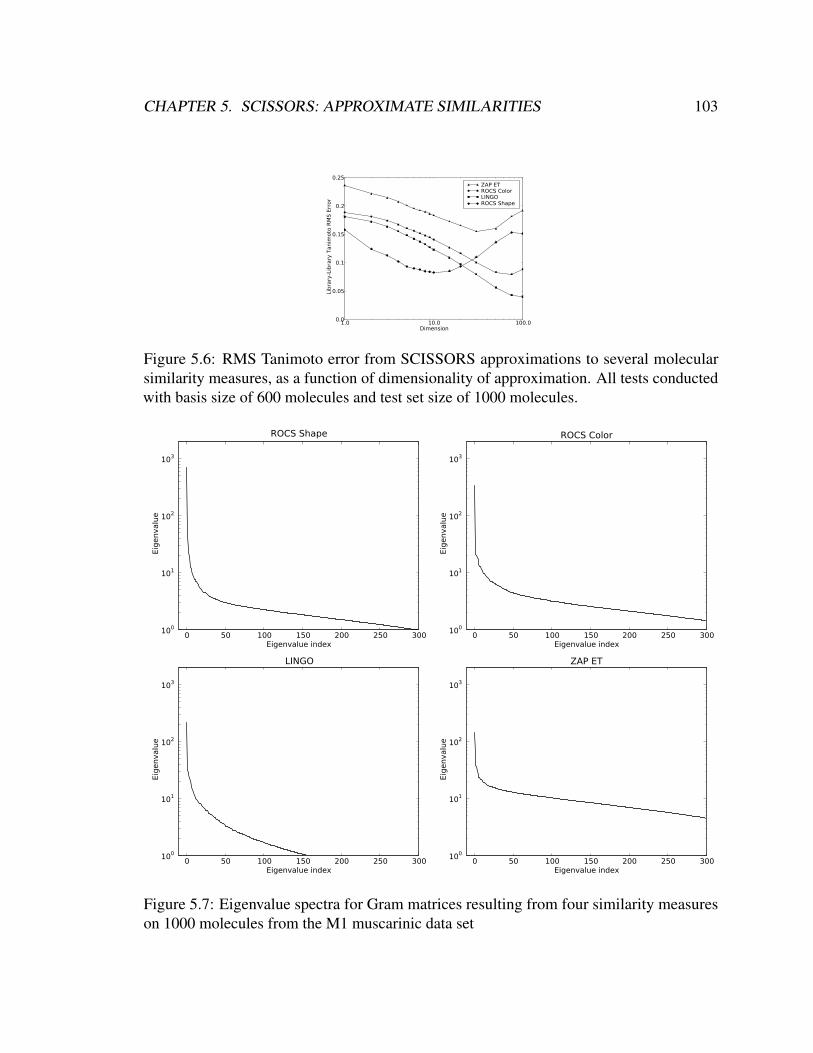
CHAPTER 5. SCISSORS: APPROXIMATE SIMILARITIES 103
1.0 10.0 100.0Dimension
0.0
0.05
0.1
0.15
0.2
0.25
Libra
ry-L
ibra
ry T
anim
oto
RM
S E
rror
ZAP ETROCS ColorLINGOROCS Shape
Figure 5.6: RMS Tanimoto error from SCISSORS approximations to several molecularsimilarity measures, as a function of dimensionality of approximation. All tests conductedwith basis size of 600 molecules and test set size of 1000 molecules.
0 50 100 150 200 250 300Eigenvalue index
100
101
102
103
Eig
envalu
e
ROCS Shape
0 50 100 150 200 250 300Eigenvalue index
100
101
102
103
Eig
envalu
eROCS Color
0 50 100 150 200 250 300Eigenvalue index
100
101
102
103
Eig
envalu
e
LINGO
0 50 100 150 200 250 300Eigenvalue index
100
101
102
103
Eig
envalu
e
ZAP ET
Figure 5.7: Eigenvalue spectra for Gram matrices resulting from four similarity measureson 1000 molecules from the M1 muscarinic data set

CHAPTER 5. SCISSORS: APPROXIMATE SIMILARITIES 104
machine details are presented in the Appendix). The precalculation time is dominated by
ROCS calculations; the spectral decomposition and least squares inference for SCISSORS
take less than 5 seconds, compared to nearly 11 000 seconds for the basis-vs-basis and
library-vs-basis ROCS computations.
A significant benefit of SCISSORS is that it calculates accurate estimates of molecular
similarity extremely rapidly once library vectors have been inferred. This is particularly true
in the case of the ROCS shape and color similarities, which are industrially important, but
expensive to calculate. We measured the OpenEye ROCS implementation’s performance at
approximately 1000 comparisons/sec per core on a 3GHz Mac Pro while performing the
basis-basis and library-basis ROCS comparisons for the above benchmark. In contrast, our
C code to evaluate SCISSORS Tanimotos (compiled with gcc 4.0.1 and GotoBLAS2 [32])
is capable of computing approximately 50 million similarities (in 64 dimensions) per second
on one core of the same CPU. With precomputed library vectors, then, SCISSORS is around
50,000 times faster than a direct calculation of Gaussian overlap.
Indeed, SCISSORS is fast enough that for very large similarity-matrix problems, it can
be faster to recalculate similarities on the fly from SCISSORS vectors than to precalculate
all similarities and read them back from disk. This leads to a significant savings in storage,
as the storage required for the molecule vectors scales as O(N), while storage for a similarity
matrix scales as O(N2). The combination of high computation speed and reduced storage
makes similarity calculations computationally feasible for datasets with N on the order of
105 to 107 for large scale virtual screening and data analysis. While SCISSORS does not
solve other issues involved with large data sets (e.g., file handling and molecule preparation),
it is able to reduce both the computational and total data storage burdens for large-scale
problems. In terms of CPU time alone, it can make difficult problems easy, and impossible
problems difficult.

CHAPTER 5. SCISSORS: APPROXIMATE SIMILARITIES 105
Step Time (sec)Basis-matrix ROCS calculation 262
Basis vector calculation (eigendecomposition) 0.33Library-vs-basis ROCS calculation 10732
Library vector calculation (least squares) 4
Table 5.1: SCISSORS precalculation step timings for 20,480 library molecules using 500molecule basis set, using one core of a 3GHz Intel Xeon-based Mac Pro
5.4 Discussion
5.4.1 Connections to Previous Work
Previous Methods to Characterize Chemical Space
Several methods have been applied in past work to characterize chemical space by learning
relevant dimensions along which chemicals vary to find vector embeddings of molecules.
In this section we discuss past work which has used multidimensional scaling and other
similar techniques to find vector embeddings of molecules based on particular similarity
representations.
Multidimensional scaling has previously been applied to chemical datasets in order to
reduce the dimensionality of binary molecular fingerprints [17, 57]. This approach has
been used for combinatorial library design; by computing coordinates for each molecule
and treating each dimension as a property, it is possible to maximize the distance among
molecules to select a maximally diverse library [57]. However, using MDS directly in this
manner is not scalable to large compound sets, as it requires a full N2 similarity matrix.
There have also been prior efforts to develop scalable versions of MDS-based methods.
One method, due to Nicholls [60], focuses on similarity metrics; that is, on similarity
measures that compute a distance between pairs of molecules, such that these distances obey
the triangle inequality. The Nicholls method, after computing coordinates for a basis set of
molecules using MDS, computes coordinates for a new non-basis molecule by triangulation
based on distances to each of the basis molecules.
The principal difference between SCISSORS and these older MDS-based methods is our
use of least-squares approximation to calculate coordinates for non-basis molecules. Least

CHAPTER 5. SCISSORS: APPROXIMATE SIMILARITIES 106
squares allows SCISSORS to scale well to large datasets, unlike the original methods using
MDS for dimensionality reduction. Furthermore, because we approximate inner products
rather than distances, and use least-squares rather than triangulation to calculate coordinates,
we do not assume that the approximated similarity measures are true metrics. In particular,
the use of least squares allows SCISSORS to calculate approximate coordinates even in
the non-metric source similarity case (in which the triangulation equations would have no
consistent solution). The SCISSORS similarity is a metric (or pseudometric, in the case of
the slack-corrected Tanimoto) approximation to the source measure.
Raghavendra and Maggiora [71] developed a symmetric-orthogonalization method
(similar in some respects to SCISSORS) to calculate vector embeddings of molecules
in an arbitrary similarity space. Like SCISSORS, the Raghavendra and Maggiora (RM)
method calculates a pairwise similarity matrix on a small set of basis molecules, uses this
to find vectors for the basis, and then projects library molecule vectors onto this space by
transforming library-basis similarity values. It is presented only as a method to describe
chemical space, and not as a method to approximate similarities. Several mathematical
limitations impact the applicability of this method for both purposes.
One critical difference is in the treatment of the basis similarity matrix, the entries
of which are Tanimotos. The RM method treats these entries as though they were inner
products; however, as equation 5.1 shows, the Tanimoto is a function of an inner product,
but not an inner product itself. This inaccuracy will distort vector spaces inferred by the
method. Furthermore, this method is unable to handle molecular similarities which do
not result in positive definite Gram matrices (i.e., non-Euclidean measures). SCISSORS
handles these in two ways. First, the use of the slack correction allows approximation of
dimensions associated with the negative eigenvalues in a non-positive-definite similarity
measure. Second, a typical use of SCISSORS will retain fewer eigenvalues/eigenvectors
(SCISSORS dimensions) than can be computed from the matrix. This allows a positive-
definite approximation of non-positive-definite measures. It also improves the statistical
reliability of our vector approximations. The RM method projects library molecules onto
the full number of dimensions computed from the basis matrix (i.e., number of dimensions
= number of basis molecules). However, as shown in 5.1 and 5.2, fitting to a number of
dimensions similar to the number of molecules leads to large approximation errors from

CHAPTER 5. SCISSORS: APPROXIMATE SIMILARITIES 107
overfitting. Thus, we argue that the SCISSORS method is more faithful to the mathematics
behind similarity coefficients, is more flexible by allowing approximation of non-Euclidean
measures, and is more accurate because it adds the ability to avoid overfitting.
Connections to Kernel PCA
Kernel principal components analysis (kernel PCA) is a nonlinear variant of principal compo-
nents analysis that, given data in some input vector space, finds the principal components of
the data in a different vector space known as the feature space [77, 78]. The dimensionality
of this feature space is often very high (possibly infinite). The computation is achieved by
the use of kernel functions, which map a pair of points in the input space to a real number
that is interpretable as the inner product of the two points in the feature space, without
requiring an explicit expansion of the points into the feature space.
In the Methods, we derived the SCISSORS algorithm from classical multidimensional
scaling. The method used in SCISSORS to derive basis vectors is also closely related to
kernel PCA (which is itself closely linked to multidimensional scaling [88]. In particular,
by transforming chemical similarity Tanimoto values to inner products, we treat trans-
formed chemical similarity functions as kernels that map molecules from some hypothetical
“molecule space” into a feature space induced by the particular similarity function. Because
the mathematical methods underlying SCISSORS are essentially identical to those of kernel
PCA, several optimality properties of kernel PCA [77] carry over to SCISSORS. As was
previously argued from the derivation from multidimensional scaling, a SCISSORS/kernel-
PCA expansion of a molecule in k-dimensions of a chemical feature space has minimum
mean-squared approximation error, compared to any other choice of k directions (e.g., as
might be derived from a truncation of a Cholesky decomposition).
Furthermore, the k directions calculated from kernel PCA have minimal representation
entropy. As a consequence, no other orthogonal basis transformation can reproduce the
given inner product matrix with the same accuracy in fewer bits. This property provides a
rigorous bound on the accuracy of vectors calculated by SCISSORS — no other method
evaluating chemical similarity inner products by dot products between real vectors can
achieve a better coverage of the variance in the training (basis) matrix with fewer bits than
used by SCISSORS.
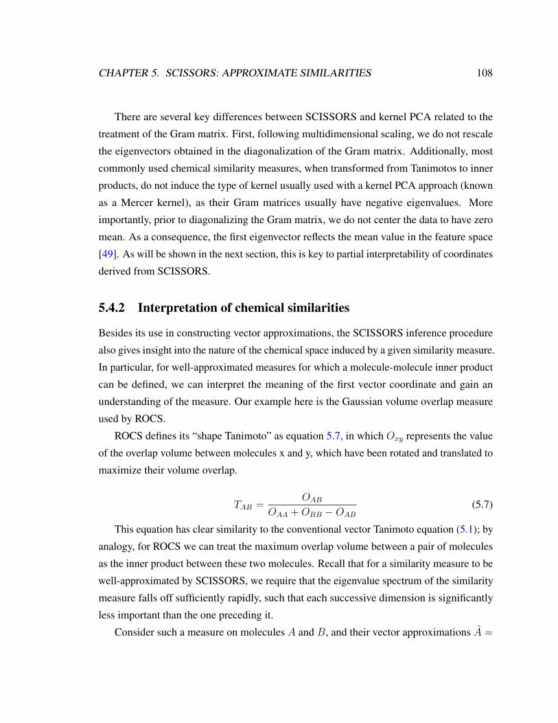
CHAPTER 5. SCISSORS: APPROXIMATE SIMILARITIES 108
There are several key differences between SCISSORS and kernel PCA related to the
treatment of the Gram matrix. First, following multidimensional scaling, we do not rescale
the eigenvectors obtained in the diagonalization of the Gram matrix. Additionally, most
commonly used chemical similarity measures, when transformed from Tanimotos to inner
products, do not induce the type of kernel usually used with a kernel PCA approach (known
as a Mercer kernel), as their Gram matrices usually have negative eigenvalues. More
importantly, prior to diagonalizing the Gram matrix, we do not center the data to have zero
mean. As a consequence, the first eigenvector reflects the mean value in the feature space
[49]. As will be shown in the next section, this is key to partial interpretability of coordinates
derived from SCISSORS.
5.4.2 Interpretation of chemical similarities
Besides its use in constructing vector approximations, the SCISSORS inference procedure
also gives insight into the nature of the chemical space induced by a given similarity measure.
In particular, for well-approximated measures for which a molecule-molecule inner product
can be defined, we can interpret the meaning of the first vector coordinate and gain an
understanding of the measure. Our example here is the Gaussian volume overlap measure
used by ROCS.
ROCS defines its “shape Tanimoto” as equation 5.7, in which Oxy represents the value
of the overlap volume between molecules x and y, which have been rotated and translated to
maximize their volume overlap.
TAB =OAB
OAA +OBB −OAB
(5.7)
This equation has clear similarity to the conventional vector Tanimoto equation (5.1); by
analogy, for ROCS we can treat the maximum overlap volume between a pair of molecules
as the inner product between these two molecules. Recall that for a similarity measure to be
well-approximated by SCISSORS, we require that the eigenvalue spectrum of the similarity
measure falls off sufficiently rapidly, such that each successive dimension is significantly
less important than the one preceding it.
Consider such a measure on molecules A and B, and their vector approximations A =

CHAPTER 5. SCISSORS: APPROXIMATE SIMILARITIES 109
[a0 · · · an] and B = [b0 · · · bn]. Because SCISSORS is able to approximate the measure
well, it is true that 〈A,B〉 ≈⟨A, B
⟩. The assumption that the measure is approximated
well implies (by the discussion in section on generalizability) that the eigenvalue spectrum
falls off rapidly. This in turns means that the first coordinate will be the dominant component
of the inner product (since further coordinates are decreasingly important), or formally,
that 〈A,B〉 ≈⟨A, B
⟩≈ a0b0. In the special case in which A = B (the self-similarity of
molecule A), 〈A,A〉 ≈ a20.
For the ROCS similarity measure, this implies that the first coordinate of the vector for
a given molecule, and therefore the first principal coordinate of the shape space induced
by the measure, is approximately equal to the square root of the molecular volume. This
is illustrated in Figure 5.8(a), which plots the first coordinate of many molecule vectors
inferred by SCISSORS on the ROCS shape overlap quantity against their molecular volumes.
The lines show that the data are well-fit by a square-root function multiplied by a constant
that represents the relative importance of molecular volume to the whole similarity measure.
This demonstrates that shape-based virtual screening is largely controlled by differences in
molecular volume, which correlates very closely with molecular weight (Figure 5.8(b)).
As explained by analogy to kernel PCA, this first coordinate (which for ROCS is
approximately equal to the square root of the molecular volume) reflects the mean location
of the molecules in the feature space learned from the similarity measure. We do not
know whether a similar chemically-interpretable understanding of the second and later
eigenvectors (projections onto which are the molecular coordinates) exists. It has been
demonstrated [7] that the eigenvectors calculated by kernel PCA converge, in the large-basis-
limit, to eigenfunctions of a linear operator on the underlying kernel. These in a sense reflect
a functional basis for the kernel (or similarity measure). However, in general, coordinates in
a kernel feature space as calculated by kernel PCA are not required to have preimages in the
input space [77]; making matters worse, in the SCISSORS case (similarity kernels operating
on molecules), it is not even clear what the input space is! Therefore, we do not have a
mathematical derivation for the chemical meaning behind particular coordinates. While it is
possible that empirical examination of large molecule sets and their SCISSORS coordinates
may uncover such interpretations, interpretability is not crucial to our target application (fast
similarity estimation), and we have not carried out such an analysis.

CHAPTER 5. SCISSORS: APPROXIMATE SIMILARITIES 110
500 1000 1500 2000ROCS self-overlap volume (no hydrogens)
200
400
600
800
1000
1200
Square
of
SC
ISSO
RS c
oord
inate
0
y=0.37x+330.21,R2 =0.60
50
100
150
200
250
300
350
400
450
Num
ber
of
mole
cule
s
(a) Density plot of square of first coordinate of SCISSORS vectors inferred fromROCS shape overlap values versus ROCS self-overlap volume. Red line indicatesoptimal linear fit.
500 1000 1500 2000ROCS self-overlap volume (no hydrogens)
200
300
400
500
600
Mole
cula
r w
eig
ht
(no h
ydro
gens)
y=0.25x+57.97,R2 =0.83
0
200
400
600
800
1000
1200
1400N
um
ber
of
mole
cule
s
(b) Density plot of molecular self-volume from ROCS against molecular weight. Redline indicates optimal linear fit.
Figure 5.8: Interpretation of SCISSORS coordinates. All data from 128,371 Tanimotoscomputed on DUD test set; 500 random molecules from Maybridge used as basis.

CHAPTER 5. SCISSORS: APPROXIMATE SIMILARITIES 111
5.4.3 Insights into chemical space
An interesting result of the SCISSORS analysis is that relatively few basis molecules (on
the order of 500-1000) were sufficient to achieve accurate estimation of shape Tanimotos
for compounds in Maybridge and DUD, and that the source of these molecules (Maybridge,
Asinex, or Maybridge Fragment) made little difference for virtual screening. This finding
is paralleled by previous results. Haigh et al. demonstrated that a reference shape set of
3,119 molecules was sufficient in their “shape fingerprints” approach to reproduce shape
Tanimotos, and that these reference shapes were transferable across databases [38]. Fontaine
et al. found that a database of 2,458 reference shapes was sufficient to cover the shape
space of a one million compound single conformer data set in their “alignment recycling”
approach [27]. Thus, our results corroborate past data showing that although chemical space
is very large, the shape space of relevant druglike molecules may be fairly small, with only a
few hundred to a few thousand basis shapes providing adequate coverage of the shape space.
5.4.4 Applications — Fast library screening and clustering with SCIS-SORS
The combination of learning vectors on a small basis set with fitting of new vectors in linear
time using least-squares makes possible highly accelerated library screening. The target
scenario for such an application involves screening based on a similarity measure that is
expensive to calculate relative to the calculation of a low (order of 101 − 102)-dimensional
dot product. The SCISSORS-accelerated screening protocol follows these steps:
1. Select 500-1000 molecules at random to serve as a basis set for the library
2. Use SCISSORS to infer vectors for basis set by eigenvalue decomposition and for
library by least squares
3. For each similarity search against the library, run slow similarity method for query
molecule versus each basis molecule and learn vector
4. Screen query molecule against full library by SCISSORS vector Tanimoto
CHAPTER 5. SCISSORS: APPROXIMATE SIMILARITIES 112
The advantage to the SCISSORS protocol is that after vectors have been inferred for a
given library of molecules, each new screen only requires that the source similarity measure
be run against the basis set, not the whole library. The majority of the comparisons can be
done using the SCISSORS Tanimotos, which are thousands of times faster to evaluate.
In particular, clustering and other approaches that require the computation of a full
O(N2) similarity matrix can be dramatically accelerated by SCISSORS. Assuming a library
of size N and a basis set of size k (k � N ), using SCISSORS to compute the Tanimoto
similarities for the matrix requires only O(kN) evaluations of the slow similarity measure,
rather than O(N2). Since k can be chosen as a fixed constant, SCISSORS is asymptotically
faster in slow similarity evaluations than a straightforward similarity construction by a factor
ofN/k - potentially many thousands of times. This, combined with the asymptotic reduction
in storage space required to quickly retrieve a similarity matrix (discussed in the Results),
demonstrates that SCISSORS enables huge reductions in computational cost for large-scale
chemical matrix problems.
5.5 Conclusion
The heavy computational burden imposed by popular chemical similarity measures, com-
bined with the growing size of chemical databases, necessitates faster techniques for sim-
ilarity comparison to enable large-scale cheminformatics analyses. We have described
SCISSORS, a generic method for rapid estimation of chemical similarities that is applicable
to several popular similarity measures, including ones based on substructure comparison
(LINGO) [85] and three-dimensional shape and chemical complementarity [33, 75]. SCIS-
SORS is able to achieve high accuracy with an efficient precalculation procedure and
relatively small molecular basis set. Given precalculated molecular vectors, our method
achieves several thousandfold speedup relative to running the source similarity metric for
ROCS. We have further described a method that allows construction of a molecular similarity
matrix (an important intermediate step in several algorithms) with only a linear number of
evaluations of the source similarity measure, rather than the quadratic number normally
required.
There are several avenues for further exploration of SCISSORS and related methods.

CHAPTER 5. SCISSORS: APPROXIMATE SIMILARITIES 113
In particular, it would be interesting to examine the performance of previously-described
molecular shape basis sets [27, 38] as basis sets for SCISSORS. There is also scope for
exploration of methods that can better capture the curvature of the feature spaces induced by
certain similarity measures.
Our algorithm enables cheminformatics calculations to be performed with asymptotically
lower costs, both in terms of computation (number of slow similarity evaluations) and storage
(keeping molecule vectors on disk rather than full similarity matrices). As a consequence,
we anticipate that SCISSORS will allow a new class of extreme-scale cheminformatics
applications combining very large datasets with similarity measures formerly considered
inaccessible for large compound collections.
5.6 Appendix: Detailed Methods
5.6.1 Molecular Databases and Preprocessing
The following databases were used
• Maybridge+BBP: 56841 of 56842 molecules from Maybridge Screening Collection
(cromoglicic acid caused Omega to crash and was excluded) + 417 molecules from
a blood-brain barrier penetration dataset [54]. Molecules from Maybridge were
provided as 2-D SDF files; BBP molecules were provided as SMILES.
• Directory of Useful Decoys, release 2: 128,371 molecules provided as 3-D MOL2
files with embedded charges.
• Asinex Gold Collection: 233,795 molecules provided in 2-D SDF format.
• Maybridge Fragment Library: 473 molecules provided in 3-D MOL2 format with
embedded charges.
• PubChem Assay #677 (Discovery of novel allosteric modulators of the M1 muscarinic
receptor: Antagonist Confirmation Screen): 1,665 molecules provided in 2-D SDF
format.

CHAPTER 5. SCISSORS: APPROXIMATE SIMILARITIES 114
For standardization, all molecules (even if provided with 3-D geometry and charge infor-
mation) were converted to 2-D uncharged OEBinary format using the OpenEye OEChem
toolkit and then processed through the same pipeline. Molecules consisting of multiple
disconnected chains (e.g., acids with counterions) were reduced to a single chemical chain
using the function “OETheFunctionFormerlyKnownAsStripSalts” to keep only the largest
single chain. Molecules containing atoms other H, C, N, O, F, Si, P, S, Cl, Br, and I
were excluded, as these are the only atoms allowed in the MMFF94s force field used by
OMEGA. Protonation, tautomer, and stereochemical state (other than invertible nitrogens)
were maintained as given in the input data.
From the 2-D representation, the OpenEye Omega toolkit was used to build one 3-D
conformer, using all default settings except for MaxConfGen=50 and MaxConfs=1. This
representative conformer was used to assign charges, using the AM1-BCC charge model in
the OpenEye OEProton toolkit. Final 3-D conformers were then built using Omega with the
following parameters:
• Bondi van der Waals radii
• fromCT = False
• EnumNitrogen = True
• EnumRing = True
• BuildForceField = SearchForceField = mmff94s Trunc
• EnergyRange = “5.0, 10.0, 15.0, 20.0, 25.0”
• MaxConfGen = 3000
• MaxConfRange = 50, 100, 200 (multi-conformer molecules only)
• MaxConfs = 1 (single-conformer molecules only)
• RangeIncrement = 3
• RMSRange = “0.5,0.75,1.0,1.5”

CHAPTER 5. SCISSORS: APPROXIMATE SIMILARITIES 115
For the Maybridge+BBP dataset, both multi-conformer and single-conformer molecules
were built; for all others, only single-conformer representations were used. These datasets
were already in use for other ongoing drug discovery projects, and thus were not re-built for
this study.
All molecule files used as input to ROCS, LINGO, ZAP, and the SCISSORS training
routines were stored as 3-D OEBinary files.
5.6.2 Software versions
The Maybridge+BBP data set was prepared using OEChem 1.5.1 for file parsing, OEOmega
2.2.1 for conformer generation, and OEProton 1.2.1 for charge assignment. All other data
sets were prepared using OEChem 1.6.1, OEOmega 2.3.0, and OEQuacPac (the renamed
OEProton) 1.3.1.
ROCS shape and color similarities were calculated by the OpenEye OEShape toolkit,
version 1.7.0. LINGO similarities were calculated using OEChem 1.6.1. ZAP ET similarities
were calculated using OEZap 2.1.0.
Benchmarking of SCISSORS similarities was done using an implementation written in
Python and C, using Python 2.5.2, Numpy 1.1.0, and GotoBLAS2 1.13. Most calculations
were performed using an older implementation of SCISSORS written in pure Python and
Numpy; performance benchmarking was done using a newer implementation of SCISSORS
Tanimotos written in C using GotoBLAS2. C code was compiled using gcc 4.0.1.
5.6.3 Software settings for similarity calculations
ROCS shape and color similarities for all accuracy tests except the virtual screening test
were calculated using the Analytic overlap method, the Implicit Mills-Dean color forcefield,
with color optimization enabled, ignoring hydrogens, and using exact atomic radii (rather
than coercing all radii to the carbon radius). For each pair of molecules, the best overlay
was chosen from the set of all conformer pairs (for multiconformer matches) and ROCS
starting positions by selecting the overlay with the highest Combo score. The shape and
color Tanimoto values from this overlay were used as the representative Tanimoto values for
that particular pair.
CHAPTER 5. SCISSORS: APPROXIMATE SIMILARITIES 116
For virtual screening, ROCS was run on the DUD molecules with the Grid overlap
method, ignoring hydrogens, and with no color force field (as only the shape Tanimoto was
being approximated).
For the performance benchmark (in which we measured the time to construct a SCIS-
SORS representation of a 20,480 molecule library), ROCS/OEShape was run in Analytic
overlap mode with no color force field (shape only), and default settings otherwise.
LINGO similarities were calculated using the OELingoSim module in OEChem. Aro-
maticity (using OpenEye aromaticity model) and chirality were perceived on molecules
from their 3-D structures; LINGO similarities were then calculated based on an isomeric
canonical SMILES representation.
ZAP electrostatic Tanimotos were calculated using the OEET module in OEZap. First,
molecules were overlaid into their optimal overlaid pose using ROCS using the same settings
as for shape/color similarity. OEET’s default settings for Tanimoto similarity were used
to calculate the electrostatic similarity, based on the AM1-BCC charges calculated during
molecule setup.
5.6.4 Performance benchmarking setup
Performance benchmarking for ROCS and SCISSORS was run on a Mac Pro with 2 x 3GHz
Quad-Core Intel Xeon CPUs (Core 2 architecture) and 16GB of DDR2 667MHz fully-
buffered memory, running OS X 10.5.8. Both the ROCS and SCISSORS benchmarking
scripts were written in Python and executed on a 32-bit build of CPython 2.5.2. All
benchmarks were conducted as single-CPU tests.
ROCS was called from within a Python script using the OpenEye OEShape toolkit
and greater than 97% of the execution time was spent inside the OEBestOverlay.Overlay
function (which calculates the optimal overlap).
SCISSORS operations other than Tanimoto calculations were performed using standard
operations in Numpy 1.1.0, as downloaded in binary form from numpy.scipy.org. The C
module for SCISSORS Tanimoto calculation was built against GotoBLAS2 1.13, using
gcc 4.0.1, with the following performance-relevant compiler options: g++ -arch i386 -
fno-strict-aliasing -Wno-long-double -no-cpp-precomp -fno-common -DNDEBUG -msse

CHAPTER 5. SCISSORS: APPROXIMATE SIMILARITIES 117
-msse2 -msse3 -march=core2 -mfpmath=sse -O3. SCISSORS Tanimoto calculation times
were computed over 4,096 x 262,144 Tanimotos, calculated in blocks of 4,096 x 32,768, in
64 dimensions.

Chapter 6
Error Bounds on SCISSORS
Abstract
The SCISSORS method for approximating chemical similarities has shown excellent empiri-
cal performance on a number of real-world chemical data sets, but lacks theoretically-proven
bounds on its worst-case error performance. The work in this chapter first proves reductions
showing SCISSORS to be equivalent to two previous kernel methods: kernel principal
components analysis and the rank-k Nystrom approximation of a Gram matrix. These
reductions allow the use of generalization bounds on these techniques to show that the
expected error in SCISSORS approximations of molecular similarity kernels is bounded in
expected pairwise inner product error, in matrix 2-norm and Frobenius norm for full kernel
matrix approximations, and in RMS deviation for approximated matrices.
118

CHAPTER 6. ERROR BOUNDS ON SCISSORS 119
6.1 Introduction
The SCISSORS method is a technique for accelerating chemical similarity search by trans-
forming Tanimoto similarity scores to inner products, computing a metric embedding for
a small “basis set” of molecules that optimally reconstructs the given inner products, and
then projecting remaining non-basis “library” molecules into this vector space [40]. SCIS-
SORS similarities are then computed as Tanimotos on these embedded vectors. Significant
speedups can be achieved for certain similarity measures (those which are expensive to
compute, and have highly concentrated eigenvalue spectra) for repeated queries into a static
database: the work done to compute vector projections for each database molecule can
be amortized easily across a large number of queries. In the original SCISSORS paper,
Haque and Pande report that for a database of approx. 57,000 molecules, a basis set of
1,000 molecules and embedding dimension of 100 was sufficient to accurately reproduce
the shape similarity over the whole database.
The embedding used in SCISSORS is computed by first calculating the pairwise inner
product matrix G between all pairs of basis molecules. G is then decomposed into eigenvec-
tors V and eigenvalues along the diagonal of a matrix D; the vector embedding for the basis
molecules lie along the rows of matrix B in the following equation:
G = BBT = V DV T = V D1/2D1/2V T
∴ B = V D1/2 (6.1)
The rank of the approximation can be controlled by ordering the eigenvalues in order of
decreasing value, setting all eigenvalues below a certain desired count to zero, and truncating
these zero dimensions in the resulting vectors.
While SCISSORS appears to have good empirical performance, it lacks theoretically-
rigorous guarantees on its approximation. In this chapter, theoretical bounds on the SCIS-
SORS approximation error will be derived by reducing SCISSORS to previously-described
kernel methods from machine learning.
CHAPTER 6. ERROR BOUNDS ON SCISSORS 120
6.2 Preliminaries
6.2.1 SCISSORS as a kernel method
The key insight of the SCISSORS technique is that molecular similarity measures, after
appropriate transformation, can be treated as kernel functions taking pairs of molecules
to scalar values that can be interpreted as inner products. The SCISSORS pipeline can be
roughly segmented into the following operations:
1. Convert Tanimotos to inner products (basis-vs-basis or library-vs-basis)
2. Compute a vector embedding on the inner products (by eigendecomposition or least-
squares)
3. Compute vector-space inner products (standard dot product in <N )
4. Convert vector-space inner products to Tanimotos using standard vector Tanimoto
equation
Steps 1 and 4 in this pipeline involve ratios of inner products (or kernel values), and as
such, introduce nonlinearities into the analysis. However, if one assumes that exact kernel
values are given or easily obtained (as demonstrated for the shape overlap volume in [40]),
and that the goal is to directly approximate these kernel values rather than the Tanimoto, then
SCISSORS directly resembles a typical kernel method. Therefore, in this chapter, we will
consider only the error in these inner-product-space stages, rather than error introduced at
the Tanimoto stages. Accordingly, we replace the notion of a “molecular similarity function”
with that of a “molecular similarity kernel”, which can be thought of as the composition of a
similarity function with the Tanimoto-to-inner-product operation from SCISSORS.
The following lemma will be useful in demonstrating the equivalence of SCISSORS to
various other kernel methods.
Lemma 6.1 (SCISSORS library vectors are projections onto eigenvectors of the basis
inner product matrix). Given an N ×N SCISSORS basis inner product matrix (that is, a
similarity matrix post-Tanimoto-to-inner-product conversion) K. Let the eigenvalues (resp.
eigenvectors) of K be denoted λi and Vi, with eigenvalues sorted in descending order of

CHAPTER 6. ERROR BOUNDS ON SCISSORS 121
value. Let the matrix of all eigenvectors be named V = [V1V2 · · ·VN ]. The SCISSORS
vector w for a new molecule with library-vs-basis inner product vector L, in d dimensions,
is defined by the expression:
w =
λ−1/21 〈V1, L〉λ−1/22 〈V2, L〉
...
λ−1/2d 〈Vd, L〉
(6.2)
Proof. Let the result of equation 6.1 be denoted B, the full-dimension basis vector matrix.
Let the restriction of B to d dimensions be denoted B′; this can be defined by B′ = V D1/2R
with the restriction matrix R defined by:
R =
[Id×d
0N−d×d
]
Where Id×d is the d× d identity matrix, and 0 is a zero matrix of appropriate dimensions.
The desired library vector w is then defined by the least-squares solution to the equation
B′w = L. This can be solved analytically:
w =(B′TB′
)−1B′TL
=(RTD1/2V TV D1/2R
)−1RTD1/2V TL
=(RTDR
)−1RTD1/2V TL
Solve for each part of this separately (with Dd and DN−d denoting corresponding blocks
of matrix D:
RTDR =[I 0
] [Dd 0
0 DN−d
][I
0
]= Dd = diag ([λ1, λ2, · · · , λd])
∴(RTDR
)−1= D−1d = diag
([λ−11 , λ−12 , · · · , λ−1d
])

CHAPTER 6. ERROR BOUNDS ON SCISSORS 122
w = D−1d
[Id 0
] [D1/2d 0
0 D1/2N−d
]V TL
= D−1d
[D
1/2d 0
]V TL
=[D−1/2d 0
]V TL
w =
λ−1/21 〈V1, L〉λ−1/22 〈V2, L〉
...
λ−1/2d 〈Vd, L〉
6.2.2 Assumptions
The analysis in this chapter will rest on the following assumptions:
• SCISSORS is given molecular similarity kernel values, not Tanimotos, to analyze.
While the conversion from Tanimoto to inner product will introduce distortion (partic-
ularly if different molecules x and y have very different values of κ(x, x) and κ(y, y)
for similarity kernel κ, we will not consider this distortion here.
• It is assumed that the similarity kernel κ is symmetric positive semidefinite (SPSD).
Similarity kernels that are not SPSD are not Mercer kernels and some proofs will
fail in the presence of negative kernel eigenvalues. However, given non-SPSD κ, the
results of this chapter can still be applied to a modified kernel κ′, the nearest SPSD
approximation to κ. If κ is symmetric but indefinite, then certain divergence terms
can be easily calculated between the kernel matrices K and K ′ induced by κ and κ′:
– ||K −K ′||2 = absolute value of the negative eigenvalue with largest magnitude
– ||K −K ′||F =∑λ2<0, where λ<0 are the negative eigenvalues
CHAPTER 6. ERROR BOUNDS ON SCISSORS 123
• It is assumed that kernel values are exactly computable. In particular, the case in
which kernel values themselves are subject to noise or inexactitude is not considered
here. However, the following chapter does treat this case.
Under these assumptions, it is possible to bound the additional error made by SCISSORS
in choosing a small random basis rather than using the eigendecomposition of the full kernel
matrix over the entire library. Two different types of bounds will be shown in this chapter,
arising from reductions to two different kernel methods: kernel principal components
analysis, and the rank-k Nystrom approximation.
6.3 Reduction of SCISSORS to Kernel PCA
6.3.1 Overview of Kernel PCA
Kernel principal components analysis [77, 78] is a generalization of traditional principal
components analysis from the data space to a feature space defined by a Mercer kernel
function κ. Given a sample of N data points, kernel PCA computes up to N directions of
maximum variance of the data, in the kernel’s feature space. Points can then be projected
into this N -dimensional subspace by a projection of their kernel values against the original
(training) data points; thus, kernel PCA can be considered to perform a metric embedding of
data points into a subspace of the feature space defined by a given kernel.
Similar to traditional (linear) PCA, kernel PCA can be preceded by a centering step, in
which the data are centered in feature space; this ensures that the data mean is not reflected
in the recovered coordinates. However, the uncentered case has relevance to SCISSORS, so
we now proceed to derive the kernel PCA algorithm without data centering (following the
approach of Scholkopf [77]).

CHAPTER 6. ERROR BOUNDS ON SCISSORS 124
6.3.2 Derivation of kernel PCA
Given a set of data points xi, i ∈ [1, · · · , `], and a Mercer kernel κ(x, y), defined by
κ(x, y) = 〈Φ(x),Φ(y)〉 for some feature-space projection Φ. Consider the feature covari-
ance matrix C:
C =1
`
∑j=1
Φ(xj)Φ(xj)T
Let the eigenvalues and eigenvectors of C be named λk and Vk respectively such that
∀k λV = CV . All such Vi must lie in the span of Φ(x1) · · ·Φ(x`). Thus the following
system is equivalent:
λ(Φ(xk) · V ) = (Φ(xk) · CV ) ∀k
and there exist a1 · · · a` such that
V =∑i=1
aiΦ(xi)
Defining matrix Kij = 〈Φ(xi),Φ(xj)〉 and vector α = [a1 · · · an]T we get `λKα =
K2α, so we solve the eigenvalue problem `λα = Kα. Solutions λk, αk correspond to
eigenvalues/vectors of the kernel matrix.
We normalize the resulting solutions by requiring that the feature-space eigenvectors
(Vk) be unit magnitude. This implies:
∑i=1
∑j=1
aki akj 〈Φ(xi),Φ(xj)〉 =
⟨αk, Kαk
⟩= λk
⟨αk, αk
⟩= 1
We can compute the projection of a new data point x onto the feature-space correlation
matrix eigenvectors Vk by:
〈Vk,Φ(x)〉 =∑i=1
aki 〈Φ(xi),Φ(x)〉

CHAPTER 6. ERROR BOUNDS ON SCISSORS 125
So for d eigenvectors, the projected KPCA coordinate vector w is:
w = KPCA{x} =
∑
i a1i 〈Φ(xi),Φ(x)〉∑
i a2i 〈Φ(xi),Φ(x)〉
...∑i a
di 〈Φ(xi),Φ(x)〉
Equivalently:
L = [〈Φ(x1),Φ(x)〉 , · · · , 〈Φ(x`),Φ(x)〉]T
w = KPCA{x} = [⟨α1, L
⟩, · · · ,
⟨αd, L
⟩]T
6.3.3 Reduction Proof
We now demonstrate that SCISSORS is equivalent to kernel PCA performed without data
centering.
As proven in Lemma 6.1, the SCISSORS vector w corresponding to a library molecule
is defined by weighted inner products between the eigenvectors of the kernel matrix and
the library-versus-basis inner product vector L. Define new vectors V ′i = λ−1/2i Vi. Recall
that the kernel matrix and vector L are already identical between methods, and both V ′i and
αi are defined to be eigenvectors of the kernel matrix. To prove equivalence, all that is left
to prove is that the SCISSORS projection vectors V ′i have the same normalization as the
KPCA αi; KPCA requires λk⟨αk, αk
⟩= 1.
Proof. We hypothesize that V ′k = αk. Then:
λk 〈V ′k , V ′k〉 = λk
⟨λ−1/2k Vk, λ
−1/2k Vk
⟩= λkλ
−1k 〈Vk, Vk〉
= 1

CHAPTER 6. ERROR BOUNDS ON SCISSORS 126
6.4 Reduction of SCISSORS to the Nystrom Rank-k Ap-
proximation
6.4.1 Overview of the Nystrom Method
In many large-scale machine learning methods, the computation and eigendecomposition of
very-large scale kernel matrices is a bottleneck, as the time complexity of eigendecompo-
sition scales as O(N3). Williams and Seeger introduced a method, based on the Nystrom
approximation from integral equation theory, to compute a low-rank approximation to a
large kernel matrix, based on computing approximate eigenvectors for the entire matrix
based on a random sample of a small number of points [87]. Precisely, using notation from
Drineas et al. [24], given an n× n kernel matrix K, a desired rank k, and a number of basis
elements `, the Nystrom approximation computes Kk, a rank-k approximation to K by the
following procedure:
Algorithm Sketch 6.1 (Nystrom approximation). Given a kernel matrix K ∈ Rn×n, choose
` columns (equivalently, ` basis/landmark input points) [b1, b2, · · · , b`] to obtain matrices C
and W :
C =
K1b1 K1b2 · · · K1b`
K2b1 K2b2 · · · K2b`...
... . . . ...
Knb1 Knb2 · · · Knb`
W =
Kb1b1 Kb1b2 · · · Kb1b`
Kb2b1 Kb2b2 · · · Kb2b`...
... . . . ...
Kb`b1 Kb`b2 · · · Kb`b`
Let Wk be the best rank-k approximation to matrix W and W+k be the Moore-Penrose

CHAPTER 6. ERROR BOUNDS ON SCISSORS 127
pseudoinverse of Wk. Then the rank-k Nystrom approximation to matrix K is defined by:
Kk = CW+k C
T
6.4.2 Preliminaries
Consider a SCISSORS computation of full pairwise similarity over some large set of
moleculesM. Partition this set, by random selection without replacement, into a basis set
B and a library set L. Then, the matrix W in Algorithm 6.1 corresponds to the SCISSORS
basis inner-product matrix on B; similarly, C is an aggregation of transposed library-vs-basis
inner-product vectors. To prove the equivalence of SCISSORS and the Nystrom method, we
will demonstrate that the inner-product matrix computed by the SCISSORS-approximated
vectors is identical to that computed by the Nystrom method. It is sufficient to show (by
Lemma 6.1) that CW+k C
T , the Nystrom-approximated Gram matrix, factorizes as SkSTkwhere:
STk = D1/2k
V T1
V T2...
V Tk
CT (6.3)
Sk is the matrix with library (and basis) vectors along the rows, so SkSTk is the SCISSORS-
approximated Gram matrix. The following lemma is helpful for the proof:
Lemma 6.2 (The pseudoinverse of Wk). W+k = V D−1k V T , where V = [V1V2 · · ·Vk],
the matrix formed from the first k columns of the basis matrix eigenvectors, and D−1k =
diag[λ−11 , λ−12 , · · · , λ−1k ], the diagonal matrix of the reciprocals of the first k eigenvalues of
the basis matrix.
Proof. The Moore-Penrose pseudoinverse of matrix A is defined to be a matrix X of

CHAPTER 6. ERROR BOUNDS ON SCISSORS 128
dimension equal to that of AT such that the following conditions hold:
AXA = A
XAX = X
AX is Hermitian
XA is Hermitian
Given that the matrix of basis row vectors in k dimensions is defined by:
B = V D1/2k =
[V1 V2 · · · Vk
]diag
[λ1/21 , λ
1/22 , · · · , λ1/2k
]Then Wk = BBT = V D
1/2k D
1/2k V T = V DkV
T . Define X = V D−1k V T . Let U = V
and E = Dk; note that columns of U are orthogonal and that all matrices are real, so that
Hermitian can be interpreted as symmetric. Then:
XWkX = UE−1UTUEUTUE−1UT
= UE−1EE−1UT
= UE−1UT
= X
WkXWk = UEUTUE−1UTUEUT
= UEE−1EUT
= UEUT
= Wk
XWk = UE−1UTUEUT
= UUT =(UUT
)T= (XWk)
T
WkX = UEUTUE−1UT
= UUT =(UUT
)T= (WkX)T
Thus, the matrix X = V D−1k V T satisfies all the Moore-Penrose properties and can be
used as the value of W+k .

CHAPTER 6. ERROR BOUNDS ON SCISSORS 129
6.4.3 Final Reduction
We must show that CW+k C
T is equal to SkSTk where STk = D−1/2k V TCT .
Proof.
SkSTk = CV D
−1/2k D
−1/2k V TCT by definition of STk
= C(V D−1k V T
)CT
= CW+k C
T by lemma 6.2
6.5 Expected error in individual inner products is boun-
ded with high probability
6.5.1 Statement of the theorem
Theorem 6.1 (Bounded expected inner product error)
Given a chemical similarity kernel κ defined over pairs of molecules from some distribution
D, such that κ(x, x) < R2 for some positive real constant R for all x ∈ D. Construct a
SCISSORS basis set from a random sample S of ` molecules drawn uniformly at random
from D. Denote by κSk the SCISSORS-approximated kernel of k dimensions from basis set
S. Then, with probability at least (1− δ)2, the expected error in SCISSORS approximation,
over pairs of independently-chosen molecules x, y ∈ D, is bounded:
0 ≤ E[κ(x, y)− κSk (x, y)
]≤
min1≤d≤k
1
`λ>d(S) +
1 +√d√
`
√√√√2
`
∑i=1
κ (si, si)2
+R2
(1
4+
√18
`ln
(2`
δ
))](6.4)
CHAPTER 6. ERROR BOUNDS ON SCISSORS 130
Where si are the basis molecules and λ>d(S) is the sum of the eigenvalues of the basis
matrix not used in SCISSORS:
λ>d(S) =∑i=k+1
λi
6.5.2 Proof Overview
The proof of Theorem 6.1 relies on a bound on the generalization error of kernel PCA
projections due to Shawe-Taylor [79]. This theorem bounds the expected residual from
projecting new data onto a sampled kernel PCA basis; we extend this proof to bound the
expected error in inner products from projecting two points onto a kernel PCA basis. Then,
the translation to SCISSORS follows trivially from the reduction of SCISSORS to kernel
PCA.
The proof relies on the following definitions from the Shawe-Taylor work [79]:
• For a sample of ` vectors S = s1, s2, · · · , s` and a kernel function κ, the sample
correlation matrix C(S) is an `× ` matrix with C(S)ij = κ(si, sj).
• Vk is the space spanned by the first k eigenvectors of C(S).
• VTk is the orthogonal complement to space Vk.
• λk is the kth process eigenvalue (true eigenvalue of the kernel operator κ, computed
over the entire distribution generating our data).
• λk is the kth empirical eigenvalue (i.e., the kth eigenvalue, in descending order of
value, of the kernel matrix on S).
• λ>k is the sum∑
i>k λk, and similarly for λ>k.
• The residual PTVk
(x) is the projection of x onto the space V Tk .
We make use of the following theorem:
Theorem 6.2 (Theorem 1 from [79])
If we perform PCA in the feature space defined by kernel κ, then over random samples of
points S s.t. |S| = ` (`-samples), for all 1 ≤ k ≤ `, if we project new data onto the space

CHAPTER 6. ERROR BOUNDS ON SCISSORS 131
Vk, the expected squared residual is bounded by the following, with probability greater than
1− δ:
λ>k ≤ E[∣∣∣∣∣∣P T
Vk(Φ(x))
∣∣∣∣∣∣2]
≤ min1≤d≤k
1
`λ>d(S) +
1 +√d√
`
√√√√2
`
∑i=1
κ (xi, xi)2
+R2
√18
`ln
(2`
δ
)(6.5)
Where the support of the distribution is in a ball of radius R in feature space.
6.5.3 Proof of Theorem 6.1
Given two data vectors ~x and ~y chosen independently from a distribution D and a kernel
κ. By Mercer’s theorem, there exists a function Φ, the feature-space projection, such that
〈Φ(~x),Φ(~y)〉 = κ(~x, ~y). Let X = Φ(~x) and Y = Φ(~y). Assume ||X||2, ||Y ||2 ≤ R2 for
some positive real constant R (i.e., support of the feature-space distribution is bounded in a
ball of radius R around the origin). Given a random `-sample of vectors from D, construct
the feature-space eigenvectors/eigenvalues from kernel PCA in k dimensions. Define X‖ to
be the projection of X onto Vk, the eigenspace of chosen dimension from KPCA and X⊥ to
be the projection of X onto V Tk , the orthogonal eigenspace. Likewise define Y‖ and Y⊥.
We would like a bound on the error of inner products in the parallel eigenspace (the
KPCA space) with respect to the true inner product. We will compute this in the form
L ≤ E[X · Y −X‖ · Y‖
]≤ U .
κ(~x, ~y) = X · Y = (X‖ +X⊥) · (Y‖ + Y⊥)
= X‖ · Y‖ +X⊥ · Y⊥ +X‖ · Y⊥ +X⊥ · Y‖= X‖ · Y‖ +X⊥ · Y⊥∴ E
[X · Y −X‖ · Y‖
]= E [X⊥ · Y⊥]
With step 3 following because dot products between orthogonal eigenspaces are zero by
definition. From this, we know that L ≥ 0, since inner products are positive. It is possible
to prove a tighter lower bound, but we are here interested in the upper bound of the error

CHAPTER 6. ERROR BOUNDS ON SCISSORS 132
only: E[X⊥ · Y⊥] ≤ U . This expression can further be bounded above:
E [X⊥ ·X⊥] ≤ E [||X⊥||||Y⊥||] Cauchy-Schwarz inequality
= E [||X⊥||]E [||Y⊥||] + Cov (||X⊥||, ||Y⊥||) (6.6)
From Theorem 6.2, we know that for every δ ∈ [0, 1], sample size `, and feature-space
radius bound R, there exists some constant α such that E [X⊥ ·X⊥] ≤ α and E [Y⊥ · Y⊥] ≤α with probability greater than (1− δ)2 (since we have two independent events each of
probability ≥ (1− δ)). Using this fact we will now bound each term in equation 6.6.
Bound on E [||X⊥||]
From Theorem 6.2, we know that E [||X⊥||2] ≤ α. By Jensen’s inequality (f(E[x]) ≤E[f(x)] for convex f ):
E2 [||X⊥||] ≤ E[||X⊥||2
]≤ α
∴ E [||X⊥||] ≤√α (6.7)
Bound on Cov (||X⊥||, ||Y⊥||)
By the Cauchy-Schwarz inequality,
Cov (||X⊥||, ||Y⊥||) ≤√V [||X⊥|]V [||Y⊥|]
By symmetry, V [||X⊥|] = V [||Y⊥|], so:
Cov (||X⊥||, ||Y⊥||) ≤ V [||X⊥|] (6.8)
Since ||X⊥|| ∈ [0, R] by the assumption on support of feature distribution, E [||X⊥||]must exist; let E [||X⊥||] = γ for some γ. Under this constraint, the variance of the
distribution of ||X⊥|| is maximized by a scaled Bernoulli random variable ν with probability

CHAPTER 6. ERROR BOUNDS ON SCISSORS 133
density f :
f(x) = δ(x)(
1− γ
R
)+ δ(x−R)
γ
R
E[ν] = 0×(
1− γ
R
)+R× γ
R= γ
V[ν] = E[ν2]− E2[ν]
=(
0 +R2 γ
R
)− γ2
= γ (R− γ)
This quadratic expression is maximized by γ = R2
, so:
V [||X⊥||] ≤R2
4(6.9)
Final steps
From Theorem 6.2: for every δ ∈ [0, 1], sample size `, and feature-space radius bound
R, there exists some constant α such that E [X⊥ ·X⊥] ≤ α and E [Y⊥ · Y⊥] ≤ α with
probability greater than (1− δ)2 for all x and y sampled independently from the distribution.
E [X⊥ ·X⊥] ≤ E [||X⊥||]E [||Y⊥||] + Cov (||X⊥||, ||Y⊥||) Equation 6.6
≤ α + Cov (||X⊥||, ||Y⊥||) Equation 6.7
≤ α + V [||X⊥||] Equation 6.8
≤ α +R2
4Equation 6.9
Therefore, by substitution from Theorem 6.2, with probability greater than (1− δ)2 on
`-samples S, for any vectors X and Y independently sampled from D, the expected kernel

CHAPTER 6. ERROR BOUNDS ON SCISSORS 134
approximation error E[X · Y −X‖ · Y‖
]is bounded above by:
α +R2
4
= min1≤d≤k
1
`λ>d(S) +
1 +√d√
`
√√√√2
`
∑i=1
κ (xi, xi)2
+R2
√18
`ln
(2`
δ
)+R2
4
= min1≤d≤k
1
`λ>d(S) +
1 +√d√
`
√√√√2
`
∑i=1
κ (xi, xi)2
+R2
(1
4+
√18
`ln
(2`
δ
))
Since computing approximate inner products using SCISSORS is equivalent to comput-
ing inner products using kernel PCA (section 6.3.3), this bound also holds for SCISSORS.
6.6 The error in SCISSORS-approximated Gram matri-
ces is bounded in 2-norm, Frobenius norm, and RMS
deviation
6.6.1 Statement of Theorems
Given a chemical similarity kernel κ and a set of n input molecules drawn from some
probability distribution such that the κ(x, x) < R2 for all molecules x. Let the true kernel
matrix be denoted K and the best possible rank-k approximation to K be denoted Kk.
Compute a SCISSORS-approximated kernel matrix K based on a size-` uniform random
sample of these vectors and a k-dimensional vector expansion. Then the following three
theorems hold:
Theorem 6.3 (Bounded error 2-norm)
With probability at least 1 − δ, the error in the SCISSORS kernel matrix is worse than
the lowest possible error from a rank k-approximated kernel matrix by at most a bounded
amount in 2-norm:

CHAPTER 6. ERROR BOUNDS ON SCISSORS 135
||K − K||2 ≤ ||K −Kk||2 +2n√`R2
[1 + 2
√(n− `)2
(n− 1/2)(n− `− 1/2)log
1
δ
]
Theorem 6.4 (Bounded error Frobenius norm)
With probability at least 1 − δ, the error in the SCISSORS kernel matrix is worse than
the lowest possible error from a rank k-approximated kernel matrix by at most a bounded
amount in Frobenius norm:
||K − K||F ≤ ||K −Kk||F +
[64k
`
]1/4nR2
[1 + 2
√(n− `)2
(n− 1/2)(n− `− 1/2)log
1
δ
]1/2
Theorem 6.5 (Bounded RMS error)
With probability at least 1 − δ, the elementwise root-mean-square (RMS) error in the
SCISSORS kernel matrix is worse than the lowest possible RMS error from a rank k-
approximated kernel matrix by at most a bounded amount:
RMS{K − K} ≤ RMS{K −Kk}
+
[64k
`
]1/4R2
[1 + 2
√(n− `)2
(n− 1/2)(n− `− 1/2)log
1
δ
]1/2
6.6.2 Proof Overview
The proofs of Theorems 6.3, 6.4, and 6.5 rely on the following theorem, due to Talwalkar
[83] bounding the error of the rank-k Nystrom approximation of a Gram matrix:
Theorem 6.6 (Theorem 5.2 from [83])
Let K denote the rank-k Nystrom approximation of an n× n Gram matrix K based on `
columns sampled uniformly at random without replacement from K, and Kk the best rank-k
approximation of K. Then, with probability at least 1 - δ, the following inequalities hold for

CHAPTER 6. ERROR BOUNDS ON SCISSORS 136
any sample of size `:
||K − K||2 ≤ ||K −Kk||2 +2n√`Kmax
[1 +
√n− `n− 1/2
1
β(`, n)log
1
δ
dKmax
K1/2max
]
||K − K||F ≤ ||K −Kk||F +
[64k
`
]1/4nKmax
[1 +
√n− `n− 1/2
1
β(`, n)log
1
δ
dKmax
K1/2max
]1/2Where:
• Kmax = maxiKii
• dKmax is the maximum distance implied in K = maxi,j√Kii +Kjj −Kij
• β(`, n) = 1− (2 max{`, n− `})−1.
For SCISSORS, we are particularly interested in the case in which `� n, so β(`, n) =
1− 12n−2` and 1/β(`, n) = n−`
n−`−1/2 .
6.6.3 Proof of Theorems 6.3, 6.4, and 6.5
Given a kernel κ and a distribution of input vectors such that their distribution in the feature
space implied by κ is D, and that the support of D is contained within a ball of radius R in
feature space. Then, Kmax in the above equations is bounded above by R2 and dKmax ≤ 2R.
Note that this boundedness assumption holds for any finite sample of vectors from D, as we
can construct an empirical distribution of vectors from the sample, which will be guaranteed
to be of bounded radius.
Theorems 6.3 and 6.4 immediately follow from theorem 6.6 by applying the reduction of
SCISSORS to the Nystrom method, the definitions of Kmax and dKmax, and the assumption
above that `� n. Theorem 6.5 requires one additional step:
Lemma 6.3. Given an n× n matrix M , the root-mean-square value of each element of M,
RMS{M} is related to the Frobenius norm of M , ||M ||F by the relationship:
RMS{M} =1
n||M ||F

CHAPTER 6. ERROR BOUNDS ON SCISSORS 137
Proof.
||M ||F =
√∑i,j
Mij
RMS{M} =
√1
n2
∑i,j
Mij =1
n
√∑i,j
Mij =1
n||M ||F
Then Theorem 6.5 follows by multiplying each term of Theorem 6.4 by 1/n.
6.7 Conclusions
Reduction to existing kernel methods makes it possible to prove rigorous probabilistic
bounds on the approximation error made by SCISSORS under fairly mild restrictions on the
input molecule distribution. However, because very few assumptions are made about the
input distribution, the resulting bounds end up being very loose. For example, consider the
added RMS error from basis-sampling (Theorem 6.5) under conditions resembling those in
[40]: n = 50, 000, k = 100, l = 1, 000, with a desired confidence of 1− e−3 ≈ 95%:
[64 · 100
1000
]1/4Kmax
[1 + 2
√(50000− 1000)2
(50000− 1/2)(50000− 1000− 1/2)log e−3
]1/2≈ 3Kmax
So with 95% confidence, the RMS kernel error will be less than 3 times the maximum
value of the kernel. This is clearly a very loose result; however, it is notable that this holds
with no assumptions about the distribution of input molecules, except boundedness in the
kernel values. The performance of SCISSORS on real-world data sets is significantly better
than this worst-case estimate, indicating that the distribution of molecules in the similarity
space considered is somehow friendly to sampling-based algorithms.

Chapter 7
The Impact of Noisy KernelComputation on Low-Rank KernelApproximation Methods
Abstract
We use a perturbation approach to explore the impact of noisy or approximate computation of
kernel functions on the spectral decomposition of the resulting kernel matrix. We apply these
perturbation results to compute the elementwise error in low-rank noisy kernel approximation
by the Nystrom rank-k method, and use these results to explain its experimental performance
on noisy kernels.
138
CHAPTER 7. NOISY KERNELS AND LOW-RANK APPROXIMATION 139
7.1 Introduction
A broad range of methods in machine learning, including both supervised (e.g., support
vector machines [13]) and unsupervised (e.g., kernel PCA [78]) learning algorithms, have
been formulated to take advantage of the “kernel trick” to do learning in non-linear spaces.
These kernel methods are constructed such that, in a linear formulation, they depend only on
the inner products between pairs of input points, not on the points themselves. To kernelize
them, the Euclidean inner product is replaced by a Mercer kernel function K(·, ·): a positive
semidefinite function mapping pairs of input points to the non-negative reals. By Mercer’s
theorem, such a kernel function is equivalent to an inner product in some (possibly high- or
infinite-dimensional) space. Thus, kernel methods can implicitly compute high-dimensional
inner products from low-dimensional data. More interestingly, kernels can also be used to
apply linear learning methods to non-vectorial data, such as text [56] or chemical structures
[40]. While no natural inner product is defined on such data, kernels defined with domain-
specific knowledge can substitute for an inner product to allow machine learning on such
domains.
Much work has been done to examine the abilities of kernel methods to denoise corrupted
input data [14], but less work [1] has focused on the issue of the kernel function itself being
corrupted. Specifically, most denoising work to date has focused on the case of equation
7.1, in which input vectors X and Y are mixed with random noise sampled from some
distribution. In this work we will consider the model of equation 7.2, in which the input
data are intact, but the resulting value of the kernel is corrupt. This change has several
interesting implications; in particular, the resultant function is no longer guaranteed to be
positive semidefinite (and in general, will not be), thus making it an improper kernel.
K(X, Y )→ K(X +N1, Y +N2) (7.1)
K(X, Y )→ K(X, Y ) +N (7.2)
We will first briefly review the sources of noise in computed kernels and then, using
a perturbative approach, derive to first order the effect of kernel noise on the eigenvalues

CHAPTER 7. NOISY KERNELS AND LOW-RANK APPROXIMATION 140
and eigenvectors of the kernel matrix. The kernel method we consider in this paper is the
Nystrom rank-k approximation of a full kernel matrix [24, 87]; we thus extend the derivation
to a first-order expression for the error in a Nystrom-approximated element. Finally, we
show experimental results using kernels from chemical informatics.
7.2 Past work and the origins of noise
Most work to date has focused on kernels whose exact values are efficiently computable. In
particular, Shawe-Taylor [79] and Talwalkar [83] have proven approximation bounds on the
error incurred by low-rank approximations in kernel PCA and the Nystrom rank-k method;
however, these bounds focus on the sampling error incurred by choosing a limited number
of data elements from some distribution. A distinct question is the error incurred by the use
of kernels whose exact evaluation is intractable, such that only approximate evaluations are
available. These kernels are particularly of interest when modeling physical systems, where
the relevant inner product in function space may be evaluated by numerical integration or
require global non-convex optimization. Formally exact kernel evaluations also may become
inexact when performed on a computer, due to limited precision introducing quantization
noise and numerical error. Thus, examining of the impact of error and noise in kernel
evaluations is of interest for practitioners of kernel-based learning methods.
An example of a noisy kernel is the molecular shape similarity function of Grant
and Pickup [35], widely used in computational chemistry and drug design. This function
computes an inner product between pair of chemical molecules represented by their excluded
volume in three-dimensional space. Each molecule is represented as the union of a number
of spherical isotropic Gaussians, each one centered on an atom. The two molecules are
rotated and translated in space to maximize their volume overlap; the kernel value is then
the overlap volume between the two. This overlap volume can formally be computed by
numerical integration of equation 7.3, where each ρAi is the Gaussian on one atom. To
ease computation, equation 7.3 is transformed to equation 7.4 by the principle of inclusion-
exclusion; this summation is then truncated at second-order overlaps and used as the
objective function for numerical local optimization [33, 39].
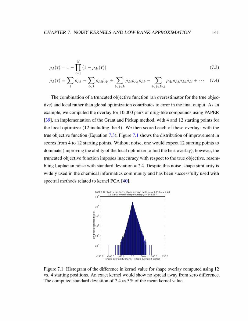
CHAPTER 7. NOISY KERNELS AND LOW-RANK APPROXIMATION 141
ρA(r) = 1−N∏i=1
(1− ρAi(r)) (7.3)
ρA(r) =∑i
ρAi −∑i<j
ρAiρAj +∑i<j<k
ρAiρAjρAk −∑
i<j<k<l
ρAiρAjρAkρAl + · · · (7.4)
The combination of a truncated objective function (an overestimator for the true objec-
tive) and local rather than global optimization contributes to error in the final output. As an
example, we computed the overlay for 10,000 pairs of drug-like compounds using PAPER
[39], an implementation of the Grant and Pickup method, with 4 and 12 starting points for
the local optimizer (12 including the 4). We then scored each of these overlays with the
true objective function (Equation 7.3); Figure 7.1 shows the distribution of improvement in
scores from 4 to 12 starting points. Without noise, one would expect 12 starting points to
dominate (improving the ability of the local optimizer to find the best overlay); however, the
truncated objective function imposes inaccuracy with respect to the true objective, resem-
bling Laplacian noise with standard deviation = 7.4. Despite this noise, shape similarity is
widely used in the chemical informatics community and has been successfully used with
spectral methods related to kernel PCA [40].
-150.0 -100.0 -50.0 0.0 50.0 100.0 150.0shape overlap(12 starts) - shape overlap(4 starts)
100
101
102
103
104
105
Bin
popula
tion (
log s
cale
)
PAPER 12 starts vs 4 starts: shape overlap deltas µ = 1.110 σ = 7.4012 starts: overall shape overlap µ = 148.087
Figure 7.1: Histogram of the difference in kernel value for shape overlay computed using 12vs. 4 starting positions. An exact kernel would show no spread away from zero difference.The computed standard deviation of 7.4 ≈ 5% of the mean kernel value.

CHAPTER 7. NOISY KERNELS AND LOW-RANK APPROXIMATION 142
Past methods have deliberately introduced structured noise into a kernel matrix to ease
computation (e.g., by sparsification) [2]. Achlioptas [1] showed that low-rank kernel approx-
imations are relatively resilient to Gaussian perturbations, and suggested that for kernel PCA
[78] in particular, replacing complicated kernels with simpler unbiased estimators can work
well. Achlioptas further suggests a rule, derived from random matrix theory, for deciding
the optimal rank of a low-rank approximation in the presence of noise. We here present an
alternative analysis, motivated by perturbative methods, that grants deeper insight into the
mechanism by which noise affects kernel methods.
7.3 Perturbing the spectral decomposition
To analyze kernel PCA and Nystrom approximation under noise, we must consider the
spectral decomposition of the kernel matrix. Our main spectral perturbation results are
summarized as Theorems 7.1 and 7.2.
Theorem 7.1If each element of an D × D kernel matrix K0 is perturbed with iid Gaussian noise
distributed as N(0, σ2), to first order, the perturbed eigenvalues λi, i ∈ 1..D, are related to
the unperturbed eigenvalues λ0i by the relationship:
λi = λ0i +N(0, σ2
)
Note that, for sufficiently large kernel matrices, as a consequence of the Central Limit
Theorem, the result of Theorem 7.1 will hold for any iid error terms of zero mean and
bounded variance.
Theorem 7.2If each element of anD×D kernel matrixK0 is perturbed with iid Gaussian noise distributed
as N(0, σ2), to first order, the perturbed eigenvectors xi, i ∈ 1..D, are a random blend of

CHAPTER 7. NOISY KERNELS AND LOW-RANK APPROXIMATION 143
the unperturbed eigenvectors x0i and are defined by the relationship:
xi = x0i +N∑j 6=i
N
(0,
σ2
(λ0i − λ0j)2
)xj
Where the λ0i are the unperturbed eigenvalues of K0, sorted in descending order.
Our perturbation analysis relies on the following fact of linear algebra [30]:
Fact 1. Given solutions xi and λ0i to the generalized eigenvalue problem K0xi = λ0iM0xi,
if we perturb matrices K0 and M0 to form new matrices K and M :
K = K0 + [δK]
M = M0 + [δM ]
For small perturbations [δK] and [δM ], the solutions xi and λi to the perturbed eigen-
value problem Kxi = λiM xi are given, to first order, by the following expressions:
λi = λ0i + xTi ([δK]− λ0i [δM ])xi
xi = xi
(1− 1
2xTi [δM ]xi
)+
N∑j 6=i
xTj ([δK]− λ0i [δM ])xi
λ0i − λ0jxj (7.5)
We are interested in the problem in which M = I , the identity matrix, and K0 is the
kernel matrix which we perturb with some random noise. Thus,
M = I
[δM ] = 0
K0xi = λ0ixi (7.6)
Proof of theorem 7.1. We begin with the perturbation equation from Fact 1. Define for
indexing convenience x = xi (this proof does not require the perturbed eigenvectors) and

CHAPTER 7. NOISY KERNELS AND LOW-RANK APPROXIMATION 144
δij = [δK]ij , and consider a system of D eigenvectors:
λi = λ0i + xT ([δK]− λ0i [δM ])x
= λ0i + xT ([δK])x
= λ0i+ xT
∑δ0jxj∑δ1jxj...∑δDjxj
λi = λ0i +
D∑k=1
xk
D∑j=1
δkjxj
Assume that the elements of [δK] are iid normal: δij ∼ N(µ, σ2) iid. Then, from
linearity of independent normal random variables:
λi = λ0i +D∑k=1
xk
D∑j=1
δkjxj
= λ0i +D∑k=1
xk
D∑j=1
N(µ, σ2
)xj
= λ0i +D∑k=1
xkN
(µ
D∑j=1
xj, σ2
D∑j=1
x2j
)
= λ0i +N
(µ∑k
∑j
xkxj, σ2∑k
∑j
x2kx2j
)
= λ0i +N
(µ∑k=j
xkxj∑k 6=j
xkxj, σ2∑k
x2k∑j
x2j
)
Further assume that our basis eigenvector x has unit magnitude (orthonormal basis).
Then:

CHAPTER 7. NOISY KERNELS AND LOW-RANK APPROXIMATION 145
λi = λ0i +N
(µ∑k=j
xkxj∑k 6=j
xkxj, σ2∑k
x2k∑j
x2j
)
= λ0i +N
(µ∑k=j
x2k∑k 6=j
xkxj, σ2∑k
x2k∑k
x2k
)
= λ0i +N
(µ∑k 6=j
xkxj, σ2
)
If the kernel noise is assumed to be zero-mean normal (µ = 0), then to first order we
have that the perturbation from the true eigenvalue is also Gaussian:
λi = λ0i +N(0, σ2
)
Proof of theorem 7.2. We want to compute the perturbed eigenvector xi of matrix K arising
from eigenvector xi of matrix K0. Let λ0i be the (unperturbed) eigenvalue of K0 corre-
sponding to eigenvector xi. Define δij ≡ [δK]ij . From Fact 1, the assumption that [M ] = I ,
and [δM ] = 0,
xi = xi
(1− 1
2xTi [δM ]xi
)+∑j 6=i
xTj ([δK]− λ0i [δM ])xi
λ0i − λ0jxj
= xi +∑j 6=i
xTj [δK]xi
λ0i − λ0jxj
= xi +∑j 6=i
1
λ0i − λ0j(xTj [δK]xi
)xj
= xi +∑j 6=i
1
λ0i − λ0j
xTj
∑d
p=1 δ1pxip∑dp=1 δ2pxip
...∑dp=1 δNpxip
xj

CHAPTER 7. NOISY KERNELS AND LOW-RANK APPROXIMATION 146
Assume δij ≡ [δK]ij ∼ N(µ, σ2) iid. Then:
xi = xi +∑j 6=i
1
λ0i − λ0j
xTj
N(µ∑
p xip, σ2∑
p x2ip
)N(µ∑
p xip, σ2∑
p x2ip
)...
N(µ∑
p xip, σ2∑
p x2ip
)
xj
= xi +∑j 6=i
1
λ0i − λ0j
(d∑q=1
xjqN
(µ∑p
xip, σ2∑p
x2ip
))xj
= xi +∑j 6=i
1
λ0i − λ0jN
(µ∑p
xip∑q
xjq, σ2∑p
x2ip∑q
x2jq
)xj
Assume µ = 0 and all unperturbed eigenvectors are unit magnitude.
xi = xi +∑j 6=i
1
λ0i − λ0jN(0, σ2
)xj
= xi +∑j 6=i
N
(0,
σ2
(λ0i − λ0j)2
)xj
7.4 First-order approximation to the kernel error
The results of Theorems 7.1 and 7.2 are sufficient to explain the noisy-kernel performance
of kernel PCA, which is typically used to find principal directions of variation in feature
space (the kernel matrix eigenvectors). Analyzing the Nystrom approximation, however,
requires one more step. Computing a rank-d approximation Kd of an N ×N kernel matrix
K using the Nystrom method is equivalent to the following procedure:
Algorithm Sketch 7.1. Computing a Nystrom approximation via kernel PCA.
1. Select B row/column indices b1, · · · , bB from K0, and select the induced B × B
submatrix β. These will be called “basis” rows, as the other elements will be projected
onto linear combinations of these landmark points.

CHAPTER 7. NOISY KERNELS AND LOW-RANK APPROXIMATION 147
2. Compute the spectral decomposition of β, retaining the eigenvectors Vi corresponding
to the top d eigenvalues λi
3. For every index `i, define the vector Li = [K(b1, `i), · · · , K(bB, `i)]T .
4. For each Li, the projection of the data item corresponding to Li onto the Nystrom
subspace is Pi =
λ−1/21 〈V1, Li〉λ−1/22 〈V2, Li〉
...
λ−1/2d 〈V1, Li〉
5. Define matrix P = [P1P2 · · ·PN ]. Then Kd = P TP .
The above procedure is equivalent to carrying out kernel PCA without centering on
a subset of the data in the kernel matrix, projecting the remainder of the data into a d-
dimensional kernel PCA subspace, and re-computing the kernel matrix using the coordinates
from kernel PCA. As a consequence, the relevant elementwise error quantity for the Nystrom
method is the error in inner products between the kernel PCA-projected vectors. Theorem
7.3 provides a first-order approximation of the elementwise error in low-rank-approximated
inner products caused by a noisy kernel.
Theorem 7.3Given an N ×N kernel matrix K and a perturbed kernel matrix K such that each element
of K −K is distributed as N(0, σ2) iid. Denote the rank-d Nystrom approximations of K
and K as Kd and Kd, respectively. Let `1 and `2 be two arbitrary data elements (row or
column indices) on which K was computed. Let P1 and P2 be the corresponding projections
onto the Nystrom subspace of K, and P1 and P2 the projections onto the Nystrom subspace
of K. Then, to first order, the error induced in the Nystrom approximation by kernel noise is

CHAPTER 7. NOISY KERNELS AND LOW-RANK APPROXIMATION 148
equal to
⟨P1, P2
⟩− 〈P1, P2〉 =
d∑i=1
[λ−1i
(〈Vi, L1〉
(N(0, σ2
)+N
(0, σ2
∑i 6=j
〈Vj, L2〉2
(λi − λj)2
)))
+λ−1i
(〈Vi, L2〉
(N(0, σ2
)+N
(0, σ2
∑i 6=j
〈Vj, L1〉2
(λi − λj)2
)))
+ξ
λi(λi − ξ)〈Vi, L1〉 〈Vi, L2〉
](7.7)
With ξ is distributed as N (0, σ2). Vi, λi, and Li are defined as in the Nystrom procedure in
Algorithm 7.1, computed on the noise-free kernel matrix K.
Proof. We will call all data elements NOT chosen in step 1 of Algorithm 7.1 “library”
elements, as opposed to the “basis” elements that were selected. From step 4 in Algorithm
7.1:
P1 =
λ−1/21 〈V1, L1〉λ−1/22 〈V2, L1〉
...
λ−1/2d 〈V1, L1〉
P2 =
λ−1/21 〈V1, L2〉λ−1/22 〈V2, L2〉
...
λ−1/2d 〈V1, L2〉
(7.8)
Using Theorems 7.1 and 7.2, we can expand the definitions of P1 and P2 to reach the
following formulas for the inner products:

CHAPTER 7. NOISY KERNELS AND LOW-RANK APPROXIMATION 149
〈P1, P2〉 =d∑i=1
λ−1/2i λ
−1/2i 〈Vi, L1〉 〈Vi, L2〉
⟨P1, P2
⟩=
d∑i=1
λ−1/2i λ
−1/2i < Vi, L1 >< Vi, L2 >
=d∑i=1
[ (λi +N(0, σ2)
)−1×⟨Vi +
∑j 6=i
N
(0,
σ2
(λi − λj)2
)Vj, L1 +Nb×1(0, σ
2)
⟩×⟨
Vi +∑j 6=i
N
(0,
σ2
(λi − λj)2
)Vj, L2 +Nb×1(0, σ
2)
⟩]
Where Nb×1(µ, σ2) is a b× 1-dimensional vector of iid normal random variables with
mean µ and variance σ2.
We will first consider each < Vi, Lj > term in isolation; to be concrete, we will look at
< Vi, L1 >. This inner product can be broken into four terms:
1. 〈Vi, L1〉: this is the desired “clean” kernel term.
2. < Vi, Nb×1(0, σ2) >. Arises from the noise in the library-vs-basis comparison.
< Vi, Nb×1(0, σ2) > =
∑k
VikN(0, σ2) = N
(0,∑k
V 2ikσ
2
)= N
(0, σ2
)since ||Vi|| = 1 (7.9)

CHAPTER 7. NOISY KERNELS AND LOW-RANK APPROXIMATION 150
3.⟨∑
i 6=j N(
0, σ2
(λi−λj)2
)Vj, L1
⟩. Arises from the noise in the basis projection eigen-
vectors.⟨∑i 6=j
N
(0,
σ2
(λi − λj)2
)Vj, L1
⟩=∑i 6=j
∑k
N
(0,
σ2
(λi − λj)2
)VjkL1k
=∑i 6=j
N
(0,
σ2
(λi − λj)2
)∑k
VjkL1k
=∑i 6=j
N
(0,
σ2
(λi − λj)2
)〈Vj, L1〉
= N
(0, σ2
∑i 6=j
〈Vj, L1〉2
(λi − λj)2
)(7.10)
4.⟨∑
j 6=iN(
0, σ2
(λi−λj)2
)Vj, Nb×1(0, σ
2)⟩
. Cross term from noise vs noise.
⟨∑j 6=i
N
(0,
σ2
(λi − λj)2
)Vj, Nb×1(0, σ
2)
⟩
=∑j 6=i
N
(0,
σ2
(λi − λj)2
)∑k
VjkN(0, σ2
)=∑j 6=i
N
(0,
σ2
(λi − λj)2
)N(0, σ2
)as in term #2
= N(0, σ2
)N
(0, σ2
∑j 6=i
1
(λi − λj)2
)(7.11)
Furthermore, we can factorize (λi +N (0, σ2))−1 to separate out the noise:
(λi +N
(0, σ2
))−1= λ−1i + ∆
∆ =(λi +N
(0, σ2
))−1 − λ−1i=
ξ
λi(λi − ξ)ξ ∼ N
(0, σ2
)(7.12)
We are now in a position to compute, to first order, the deviation in library-vs-library
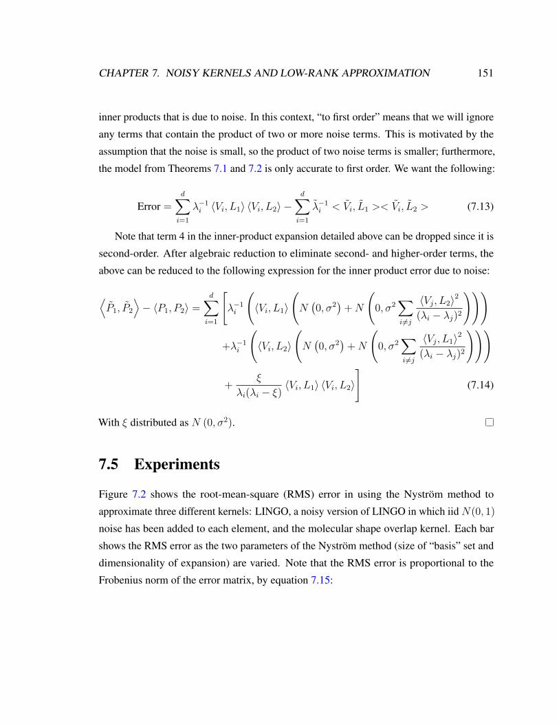
CHAPTER 7. NOISY KERNELS AND LOW-RANK APPROXIMATION 151
inner products that is due to noise. In this context, “to first order” means that we will ignore
any terms that contain the product of two or more noise terms. This is motivated by the
assumption that the noise is small, so the product of two noise terms is smaller; furthermore,
the model from Theorems 7.1 and 7.2 is only accurate to first order. We want the following:
Error =d∑i=1
λ−1i 〈Vi, L1〉 〈Vi, L2〉 −d∑i=1
λ−1i < Vi, L1 >< Vi, L2 > (7.13)
Note that term 4 in the inner-product expansion detailed above can be dropped since it is
second-order. After algebraic reduction to eliminate second- and higher-order terms, the
above can be reduced to the following expression for the inner product error due to noise:
⟨P1, P2
⟩− 〈P1, P2〉 =
d∑i=1
[λ−1i
(〈Vi, L1〉
(N(0, σ2
)+N
(0, σ2
∑i 6=j
〈Vj, L2〉2
(λi − λj)2
)))
+λ−1i
(〈Vi, L2〉
(N(0, σ2
)+N
(0, σ2
∑i 6=j
〈Vj, L1〉2
(λi − λj)2
)))
+ξ
λi(λi − ξ)〈Vi, L1〉 〈Vi, L2〉
](7.14)
With ξ distributed as N (0, σ2).
7.5 Experiments
Figure 7.2 shows the root-mean-square (RMS) error in using the Nystrom method to
approximate three different kernels: LINGO, a noisy version of LINGO in which iid N(0, 1)
noise has been added to each element, and the molecular shape overlap kernel. Each bar
shows the RMS error as the two parameters of the Nystrom method (size of “basis” set and
dimensionality of expansion) are varied. Note that the RMS error is proportional to the
Frobenius norm of the error matrix, by equation 7.15:
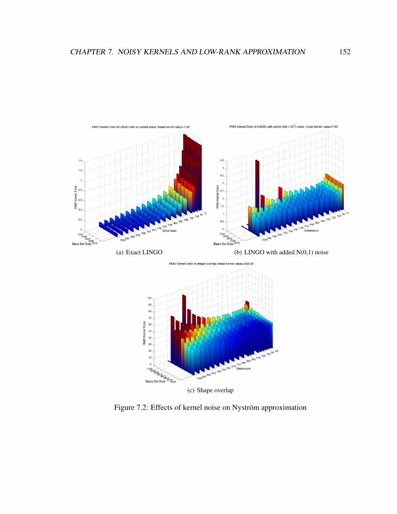
CHAPTER 7. NOISY KERNELS AND LOW-RANK APPROXIMATION 152
(a) Exact LINGO (b) LINGO with added N(0,1) noise
(c) Shape overlap
Figure 7.2: Effects of kernel noise on Nystrom approximation

CHAPTER 7. NOISY KERNELS AND LOW-RANK APPROXIMATION 153
M ∈ <m×n
||M ||F =
√∑i
∑j
M2ij
RMS(M) =
√1
mn
∑i
∑j
M2ij
∴ RMS(M) =1√mn||M ||F (7.15)
The features of these plots can be explained by combining our results with the following
bound on the error of the Nystrom approximation, due to Talwalkar [83]:
Theorem 7.4 (Theorem 5.2 of [83])
Let K denote the rank-k Nystrom approximation of an n× n kernel matrix K based on `
columns sampled uniformly at random without replacement from K, and Kk the best rank-k
approximation of K. Define β(`, n) = 1− (2 max{`, n− `})−1. If ` < n, with probability
at least 1 - δ, the following inequality holds for any sample of size `:
||K − K||F ≤ ||K −Kk||F +
[64k
`
]1/4nKmax
[1 +
√n− `n− 1/2
1
β(`, n)log
1
δ
dKmax
K1/2max
]1/2
Where Kmax = maxiKii and dKmax is the maximum distance implied by the values of K,
dKmax = maxij√Kii +Kjj −Kij .
The following fact about the Frobenius norm is also useful:
Fact 2. Given a real symmetric matrix M with singular values σi (equivalently, eigenvalues
λi:
||M ||F =
√∑i,j
M2ij =
√tr (MTM) =
√∑i
σ2i =
√∑i
λ2i (7.16)
The features of figure 7.2(a) are well-explained by Theorem 7.4. As we increase the
rank of the approximation, we account for a larger fraction of the eigenspectrum of the

CHAPTER 7. NOISY KERNELS AND LOW-RANK APPROXIMATION 154
basis matrix, reducing the magnitude of the first term in theorem 7.4 by fact 2. Error also
decreases (though to a smaller extent), as we increase the size of the basis set — this effect
can be explained by a reduction in the magnitude of the second term in the theorem.
Once noise is added to the kernel functions, theorem 7.4 is no longer sufficient to explain
the results. In particular, in both figures 7.2(b) and 7.2(c), adding dimensions only improves
the quality of the approximation to a point, after which error rises dramatically (much faster
than the fourth root of k, the rate suggested by the theorem). Furthermore, the minimum
error hits a “noise floor”, even after adding a large number of basis points. These features
are well-explained by our perturbation results.
7.5.1 Noise floors
Figure 7.2(b), shows a noise floor around an RMS error of 1 for a kernel to which we have
added N(0, 1) noise to every evaluation. An intuitive explanation is that since the kernel
evaluations are corrupted by zero-mean noise that is uncorrelated to the kernel value, the
learning algorithm will be unable to predict this noise; we would thus expect an RMS error
equal to the RMS value of the noise, which is σ.
For shape (figure 7.2(c)), the estimated noise (σ ≈ 7.4, figure 7.1) is insufficient to
explain the error floor of around 35. However, shape is not a true Mercer kernel: it has
significant negative eigenvalues [53]. Using fact 2, it is possible to compute the RMS error
due to ignoring these negative eigenvalues: approximately 27 in the large basis limit (at
which eigenvalues should be best approximated [79]). Thus, the combination of the noise
model and the negative eigenvalues is able to explain the Nystrom error floor for shape.
7.5.2 Increasing error
The second unique feature of figures 7.2(b) and 7.2(c), versus figure 7.2(a), is that for both
noisy kernels, the error eventually increases as more dimensions are used, and that this
transition can be delayed by using more basis data. Our perturbation results help to explain
this behavior.
Theorem 7.1 shows that the eigenvalues learned on a noisy kernel matrix will be equal
to the true eigenvalues, plus the added noise. This implies that as the magnitude of an

CHAPTER 7. NOISY KERNELS AND LOW-RANK APPROXIMATION 155
(a) Eigenspectra (b) Differential eigenspectra
Figure 7.3: Eigenspectra and spectral gaps for noisy LINGO and shape
eigenvalue approaches the standard deviation of the noise, the value of that eigenvalue will
become unreliable. Figure 7.3(a) plots the eigenvalue spectra for the noisy LINGO and
shape kernels for several basis set sizes, as well as the σ values for each kernel. In all cases,
a dramatic rise in error in figure 7.2 is seen when the approximation grows in dimension to
use eigenvalues whose values are around the same value as σ.
Noise in the eigenvalues of the kernel matrix determines the point where error rises
dramatically, but does not appear to correlate well with the exact location of the error
minimum. However, errors in the learned eigenvectors do have a useful effect. According
to theorem 7.2, the reliability of a learned eigenvector is determined by the separation
between its eigenvalue and the other eigenvalues of the kernel matrix: in the presence of
noise, learned eigenvectors are blends of the true eigenvector and surrounding eigenvectors,
with variance in the blending factor inversely proportional to the square of the gap between
the corresponding eigenvalues. Figure 7.3(b) plots a smoothed view of the first difference
function of the eigenvalue spectra (that is, the gap between adjacent eigenvalues) for noisy
LINGO and for shape, along with the respective noise σ values.
For shape, the differential eigenspectrum is quantitatively predictive of the error mini-
mum: the spectral gap intersects with σ = 7.4 between 200 and 300 dimensions, precisely
where the error minimum is seen in figure 7.2(c). This holds true for both 1536 and 3072

CHAPTER 7. NOISY KERNELS AND LOW-RANK APPROXIMATION 156
basis molecules, consistent with the fact that the error minimum is at approximately the same
dimensionality for both basis sets. For LINGO, the agreement is not quantitative, but is still
explanatory. Figure 7.3(b) shows the spectral gap intersecting σ = 1 around 100 dimensions
for a 1536-basis and 150 dimensions for a 3072-basis; in contrast, the minimum error is
found at 192 and 256 dimensions, respectively. While the exact count of best dimensionality
is not correct, the relative margin between the two is approximately correct. The spectral
gap criterion predicts that the 3072-basis should be able to reliably estimate an extra 50
eigenvectors, which we confirm to within the resolution of our sampling (64 dimensions).
We speculate that the reason extra vectors do not hurt for LINGO is that there are still useful
directions to be learned in this regime. In figure 7.2(a), going beyond 256 dimensions still
significantly reduces the RMS kernel error, so the true kernel has relevant information in
these dimensions. It is possible that in the noisy case, there is a tradeoff being made between
learning relevant directions in feature space, and noise in this learning, such that the net
effect is almost zero until the eigenvalue noise threshold is passed. It is also possible that
the true reason is not well explained by the first-order analysis, and requires higher-order
analysis.
7.6 Practical Recommendations
In earlier work, Achlioptas [1] suggested, when approximating an n× d matrix A, to choose
a rank k such that:
||A− Ak||2 ∼ σ√n (7.17)
Where σ2 is the mean squared entry of the error matrix A− Ak. By using fact 2, this
criterion can be converted into a form more relevant to the current work:
Criterion 7.1 (Achlioptas criterion). When computing a low-rank approximation (equiva-
lently, performing kernel PCA) on an n× n positive semidefinite kernel matrix A, let the
eigenvalues of A be named λi, i = 1 · · ·n, in descending order of value. A good choice of
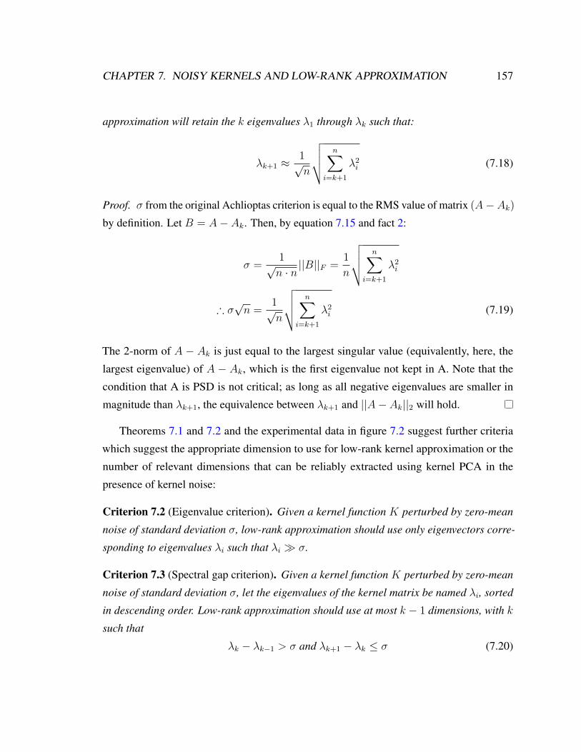
CHAPTER 7. NOISY KERNELS AND LOW-RANK APPROXIMATION 157
approximation will retain the k eigenvalues λ1 through λk such that:
λk+1 ≈1√n
√√√√ n∑i=k+1
λ2i (7.18)
Proof. σ from the original Achlioptas criterion is equal to the RMS value of matrix (A− Ak)by definition. Let B = A− Ak. Then, by equation 7.15 and fact 2:
σ =1√n · n||B||F =
1
n
√√√√ n∑i=k+1
λ2i
∴ σ√n =
1√n
√√√√ n∑i=k+1
λ2i (7.19)
The 2-norm of A − Ak is just equal to the largest singular value (equivalently, here, the
largest eigenvalue) of A − Ak, which is the first eigenvalue not kept in A. Note that the
condition that A is PSD is not critical; as long as all negative eigenvalues are smaller in
magnitude than λk+1, the equivalence between λk+1 and ||A− Ak||2 will hold.
Theorems 7.1 and 7.2 and the experimental data in figure 7.2 suggest further criteria
which suggest the appropriate dimension to use for low-rank kernel approximation or the
number of relevant dimensions that can be reliably extracted using kernel PCA in the
presence of kernel noise:
Criterion 7.2 (Eigenvalue criterion). Given a kernel function K perturbed by zero-mean
noise of standard deviation σ, low-rank approximation should use only eigenvectors corre-
sponding to eigenvalues λi such that λi � σ.
Criterion 7.3 (Spectral gap criterion). Given a kernel function K perturbed by zero-mean
noise of standard deviation σ, let the eigenvalues of the kernel matrix be named λi, sorted
in descending order. Low-rank approximation should use at most k − 1 dimensions, with k
such that
λk − λk−1 > σ and λk+1 − λk ≤ σ (7.20)

CHAPTER 7. NOISY KERNELS AND LOW-RANK APPROXIMATION 158
That is, use only eigenvectors corresponding to eigenvalues which are separated from their
neighbors by at least σ.
Acknowledgments
The authors would like to thank John Chodera for clever statistical insight. ISH acknowl-
edges support from an NSF graduate fellowship. The authors acknowledge award NSF
MRI-R2 for computing resources, funded under the American Recovery and Reinvestment
Act of 2009 (Public Law 111-5).
7.7 Appendix 1: Detailed experimental methods
7.7.1 Figure 7.1
The molecules used for this plot were the 57,248 molecule “Maybridge+BBP” dataset from
Haque [40]. 293 molecules were chosen at random as reference molecules; for each of
these, a further 1000 molecules were chosen at random and overlaid onto their references
using PAPER [39], using initialization modes 1 (4 starting points) and 2 (12 starting points,
including all 4 from mode 1). The total number of overlay volumes histogrammed in the
figure is 293,000.
Overlap volume was computed by numerical integration of equation 7.3, over all atoms
(including hydrogens) and Batsanov van der Waals radii [6]. The integration code computed
a bounding box for each molecule in an overlay, grew the box by 1 Ain each direction
(+x, -x, +y, etc.), and converted this to a cubic grid with resolution 0.3 A. Integration was
performed in single precision over the grid with more points.
7.7.2 LINGO calculations in Figures 7.2, 7.3
The molecules used for this plot were taken from the Maybridge Screening Collection
(N=56842), represented as canonical isomeric SMILES. The order of SMILES strings was
shuffled to remove local correlations between molecules adjacent in the file. Basis sets
were drawn as the first X strings in the shuffled file, for each of the basis sizes. The final

CHAPTER 7. NOISY KERNELS AND LOW-RANK APPROXIMATION 159
32,768 strings in the shuffled file were separated into 8 test sets of size 4,096. For each basis
size, dimensionality, and noise σ, all-pairs approximate kernel values were computed on
each test set and subtracted from the true kernel (or true kernel plus noise, in the case of
σ 6= 0). The square errors were then accumulated over test sets; each bar thus represents
8× 4096× 4096× 12≈ 67× 106 kernel evaluations.
Kernel evaluations were performed using a version of SIML modified to compute only
the LINGO intersection, and not the full Tanimoto [42].
7.7.3 Shape calculations in Figures 7.2, 7.3
The first 2612 basis molecules were taken from the PubChem3D shape fingerprint basis set
[27]. All remaining basis molecules were taken from a k-centers+k-medoids clustering of
PubChem3D based on ROCS Color Tanimoto, with clustering performed independently on
subsets defined by molecular volume cutoffs in the shape fingerprint basis.
The test set was constructed as 159 sets of 4000 single-conformer molecules randomly
chosen from PubChem3D. Molecules were chosen without replacement within each set,
but with replacement between sets. On average, each pair of sets shared one molecule in
common. Overlays were computed using PLASTIC, a version of PAPER [39] modified to
include support for “color” similarity analysis, and the ImplicitMillsDean color forcefield
from OpenEye ROCS. Overlays were computed optimizing for summed shape and color
similarity, but only the shape overlay scores were used to generate plots in this paper. RMS
errors were computed as for LINGO analyses, but over 159 test sets rather than 8; each bar
thus represents 159× 4000× 4000× 12≈ 1.3× 10⁹ kernel evaluations.
7.7.4 Differential eigenspectrum plot
Computed first forward difference function of each kernel matrix’s eigenspectrum by apply-
ing numpy diff operator to each eigenspectrum. Smoothed each trace for visualization using
a 9-wide moving average filter (4 previous samples, current sample, and 4 forward samples,
each with weight 1/9).

CHAPTER 7. NOISY KERNELS AND LOW-RANK APPROXIMATION 160
7.8 Appendix 2: Proof that LINGO is a proper kernel
The LINGO intersection between two strings x and y relies on first transforming each string
to a multiset [42, 85]. For the q-LINGO algorithm, each contiguous 4-character substring in
x is mapped to a multiset element; the multiplicity counts the number of times that substring
appears in x. The LINGO similarities in this work use q = 4. After transforming x and Y to
multisets X and Y , the LINGO intersection is computed as |X ∩ Y |: sum, for each element
present in X or Y , the minimum of the multiplicity of that element in X and that in Y.
For strings from an alphabet with k characters, the multiset constructed for q-LINGO
is equivalent to a histogram over kq elements: all possible q-character substrings in the
alphabet. Then, the LINGO intersection is equivalent to the histogram intersection function,
proven to be a kernel by Odone [66].
Chapter 8
Real-Time 3D Chemical SimilaritySearch over PubChem
Abstract
Similarity search over million-molecule-scale chemical databases is a bottleneck for emerg-
ing analyses in computational biochemistry. In this chapter, I show that combining special-
ized hardware and approximation algorithms overcomes this bottleneck, allowing real-time
search performance with excellent accuracy. The performance of the method is demonstrated
for 3D shape and chemical functionality (“color”) similarity on the 17 million-molecule
NCBI PubChem3D database.
161

CHAPTER 8. REAL-TIME CHEMICAL SEARCH 162
8.1 Introduction
Continuing improvements in both computer power as well as chemical high-throughput
screening have dramatically expanded the size of biochemical databases. Simultaneously,
virtual screening has become a commonly-used tool in medicinal chemistry, such that
medicinal chemists may routinely screen chemical ideas or known active hits against
large databases of existing, purchasable, or synthesizable chemical matter. As the sizes
of these databases are often beyond one million compounds, high speed is necessary to
support interactive usage of chemical similarity search, and is of critical importance to drug
discovery.
However, many useful chemical similarity measures are too slow to be used in an
interactive manner over large databases. In particular, “3D” similarity measures, which
consider the three-dimensional arrangement of atoms in a molecule rather than just atom
types and bond connectivity, are often very slow, taking on the order of 10 ms to 10 sec per
comparison. Without massive dedicated computational resources, it is impossible to support
interactive use of these tools over large-scale databases.
In this chapter, we describe how, for a particular pair of 3D similarity measures, combin-
ing special-purpose hardware (graphics processing units) and an approximation algorithm
enable interactive 3D chemical search over the 17 million-molecule PubChem3D database.
We demonstrate very high accuracy over the diverse PubChem3D library, and show that we
are able to achieve throughput of tens of millions of similarity calculations per second on a
single server, thousands of times faster than the unaccelerated calculation.
8.2 3D Similarity Measures
This section reviews shape and color similarities, two related types of chemical similarity
measures that take into account the three-dimensional nature of molecules. The versions of
shape and color we consider are based on the Gaussian model of molecular shape [35]. While
other methods for three-dimensional similarity have been considered [5, 18, 46, 48, 76], the
model based on Gaussian shape is both efficient to compute [33, 39] and has shown good
performance in drug discovery applications [75].

CHAPTER 8. REAL-TIME CHEMICAL SEARCH 163
8.2.1 Shape
Shape similarities, as used here, model the volumetric similarities between molecules. To
do this, the density function of a molecule is represented as the union of atom-centered
spherical Gaussian functions ρi [35]. While less intuitive than a “hard-sphere” model, in
which the molecule is represented as the union of finite-radius spheres centered at each atom,
the Gaussian model has the advantage of being a smooth function in space, which enables
gradient calculation and efficient evaluation.
Given two molecules A and B, the shape overlap is defined in terms of the total volume
shared by the two molecules (|A ∩ B|). Since each molecule is defined in terms of its
component atoms, the principle of inclusion-exclusion implies that this volume can be
defined in terms of second- and higher-order intersections between the atoms: |Ai ∩Bj| −|Ai ∩ Aj ∩ Bk| − |Ai ∩ Bj ∩ Bk| + |Ai ∩ Aj ∩ Bk ∩ Bl| + · · · . However, to reduce the
complexity of evaluating this objective function, implementations typically truncate this
calculation to just the second-order (pairwise overlap) term: |Ai ∩ Bj| ∀i, j [33, 39]. In
principle, the shape overlap between two molecules is defined as the global maximum of this
volume overlap objective, optimized over all rigid-body transformations of either molecule.
This optimization is usually performed by local optimizations starting from many starting
points; while not guaranteed to be globally convergent, this local optimization procedure
appears to perform well in practice.
Because the shape overlap is not a normalized measure (larger molecules will naturally
have larger overlap volumes), Gaussian shape similarity scores are usually reported in terms
of a Tanimoto coefficient:
TAB =OAB
OAA +OBB −OAB
Where Oxy is the overlap volume between molecules x and y. Since overlap volumes
are always positive, this Tanimoto is a normalized similarity between 0 and 1.

CHAPTER 8. REAL-TIME CHEMICAL SEARCH 164
8.2.2 Color
Computing chemical similarity by excluded volume, as done in shape similarity, makes the
modeling assumption that sterics are the dominant factor distinguishing molecules; if two
molecules have similar steric excluded volume, then they will be shape-similar. However,
this assumption is clearly not always true. Figure 8.1 depicts the molecular structures
as well as excluded volume for benzene and pyridine. While these two molecules have
almost identical sterics (pyridine is missing one hydrogen, and has a nitrogen whose radius
is slightly smaller than that of carbon), they have very different physical properties. In
particular, the nitrogen in pyridine confers water-solubility and a hydrogen-bond acceptor
site. For this reason, it is of interest to consider the sites of particular chemical functionalities
in space in addition to the simple steric exclusion.
(a) Benzene
N
(b) Pyridine (c) Benzene shape (d) Pyridine shape
Figure 8.1: Comparison of molecular structure and volume for benzene and pyridine
One method, known as color similarity, incorporates this chemotype matching into
the Gaussian shape framework by adding virtual atoms to represent particular chemical
functionalities. Functionalities of interest (e.g, hydrogen bonding sites and charged sites)
are defined by SMARTS (cite) strings, which identify molecular subgraphs corresponding
to the desired function. A virtual “color” atom is then added to the molecule at a site
associated with the functionality (e.g., at the centroid of the set of atoms that match the given
SMARTS pattern). A “color force field” defines the interactions of these color atoms; for
example, in the OpenEye Implicit Mills-Dean color force field, color atoms do not interact
with “real” (shape) atoms, but do have a positive interaction with atoms of their same color
type (e.g., anion-anion). The color overlap can then be computed using the same Gaussian
overlap model as in shape. The similarity between color atoms alone can be separated from

CHAPTER 8. REAL-TIME CHEMICAL SEARCH 165
that defined by the shape atoms; this leads to two different similarity measures between
molecules, the shape and color Tanimotos. It is common to consider the so-called “combo”
Tanimoto, which is the sum of shape and color Tanimotos, divided by 2 to keep it in the
[0,1] interval.
8.3 GPU Implementation of 3D Color Similarity
GPU acceleration plays a key role in our ability to deliver real-time search performance
over very large chemical databases. In previous publications [39, 41], we described the
design and implementation of PAPER (PAPER Accelerates Parallel Evaluations of ROCS),
a GPU-accelerated implementation of shape-only molecular similarity using the Gaussian
model of shape. Here, we describe the implementation of PLASTIC (PLASTIC aLigns
Atoms with Shape Theory Incorporating Color), an extension to PAPER that adds support
for color similarity calculations.
As described in section 8.2.2, color overlap interactions are computed in the same
manner as shape interactions, but on different sets of atoms, with interactions defined by a
color force field (CFF). In PLASTIC, shape and color are unified, with shape defined by
an implicit CFF rule adding a positive interaction between “shape” type atoms; the only
difference between shape atoms and color atoms of other types is that shape atoms can have
distinct radii (e.g., hydrogen and carbon will typically not be modeled with the same radius),
whereas other color types are usually defined with identical radii (e.g., all anion virtual
atoms have the same radius). However, this distinction is an implementation detail and not
critical to the method.
Three principal changes are required to implement color on the GPU: two involving
data structures and one in the core algorithm. In PAPER, each molecule uploaded to the
GPU is represented by a scalar count of atoms, 3 arrays containing coordinates of each
atom in the x, y, and z axes, and a final array containing a precomputed function of each
atom’s radius. In PLASTIC, the atom count scalar is extended to a vector. The first element
of the vector contains the total number of atoms in the molecule (shape and all virtual
types); each subsequent element contains the number of atoms of a particular type. An
additional CFF data structure is also uploaded to the GPU, defining the interactions in the

CHAPTER 8. REAL-TIME CHEMICAL SEARCH 166
CFF (e.g., anion-anion) and their weights. The weights are scalar multipliers controlling the
contribution of each interaction to the final objective score: O(a, b) =∑wiOi(a, b), where
O(a, b) is the objective between molecules a and b, wi is the weight of interaction i, and
Oi(a, b) is the overlap between a and b considering only interaction type i.
The final GPU-side change from PAPER to PLASTIC is to the objective/gradient
evaluation loop. In PAPER, all pairs of atoms from the reference and fit molecules contribute
interactions to the final overlap value. However, with the addition of a color force field, this
is no longer true: typically, for example, shape and color atoms would not interact with each
other. Thus, in PLASTIC with a typical CFF, the interaction matrix is block-diagonal, rather
than full. Using the PAPER interaction loop (in which every term of the interaction matrix
is evaluated) would be highly wasteful of computation. Instead, in PLASTIC a PAPER-
style interaction loop is embedded in an outer loop over the interaction terms in the CFF;
iterations of the outer loop are separated by a thread barrier (CUDA syncthreads).
This strategy means that only valid atom pairs are evaluated. However, because there are
typically very few color atoms of any given type in a molecule, the evaluation of color terms
is inefficient on the GPU, as there are usually more available scalar processing units (CUDA
threads) than there are atom-pair interactions for color interactions. In principle, it would
be possible to run multiple interactions simultaneously, without the barrier, but this has not
been implemented. Even with this inefficiency, we achieve typical performance of 15,000
shape+color overlay optimizations/sec for PLASTIC on the PubChem3D database, on an
NVIDIA GeForce GTX 480.
8.4 Fast Similarity Approximation by Metric Embedding
The SCISSORS technique is an approximation technique to rapidly approximate chemical
similarities by precomputing vector embeddings for molecules in a static database, and is
generalizable to many similarity measures, given technical conditions on their eigenvalue
spectra [40]. We apply the SCISSORS method to enable rapid shape and color searches on
PubChem3D; in this section we briefly review the relevant details behind SCISSORS.
The first step in computing SCISSORS-approximated Tanimotos on a large chemical
database of size N is to select a “basis set” of molecules from the database, of size k,
CHAPTER 8. REAL-TIME CHEMICAL SEARCH 167
where k is typically much less than N ; the original SCISSORS paper suggests that random
sampling of the database is a good way to pick a basis. Similarities are then computed
among all pairs of molecules in the basis set, stored in a matrix G, and converted to inner
products using the relation:
〈A,B〉 =2TAB
1 + TAB
A spectral decomposition of G, G = V DV T is then computed, and a desired dimension
d for the vector space is chosen. The eigenvalues in D are sorted in descending order (and
corresponding eigenvectors are sorted), and all eigenvalues other than the top d are set to
zero. The vector space representation for the basis molecules is then equal to the first d
columns of the matrix V D1/2, where the vector for the ith basis molecule is the ith row of
the matrix. This spectral decomposition was proven to be the least-squares optimal choice
to represent the molecules’ computed inner products, under the d-dimensional constraint.
To compute the vectors for a “library”, or non-basis molecule, that molecule is compared
against each basis molecule, the similarities are converted to inner products using the above
relation, and the inner products are stored in a vector L. The vector x representing that
library molecule is computed by solving the linear least-squares equation V D1/2x = L.
Finally, the SCISSORS-approximated Tanimoto for a given pair of molecules a and b is
computed using the vector Tanimoto relation on their vectorial representations A and B:
Tab =〈A,B〉
〈A,A〉+ 〈B,B〉 − 〈A,B〉
On any given dataset and similarity measure, SCISSORS has three tunable parameters:
the size of the basis set used, the choice of basis molecules given a fixed basis size, and
the desired dimensionality of approximation. In the remainder of this chapter, we sample
this parameter space and show that we are able to find SCISSORS parameters that allow
accurate approximation of shape and color Tanimotos on a large (>17M molecule), diverse
chemical dataset.

CHAPTER 8. REAL-TIME CHEMICAL SEARCH 168
8.5 Materials and Methods
8.5.1 Databases
To demonstrate the performance and accuracy of our techniques on a large, diverse chemical
library, we will use the PubChem3D database [10], which contains single-conformer 3D
models of (at the time of the work) 17,093,120 small molecules, approximately 90% of
the molecules in the entire NCBI PubChem Compound collection. PubChem3D represents
a broad swath of both druglike and non-druglike organic chemistry space, and therefore
demonstrates the generalization performance of our techniques onto diverse libraries.
8.5.2 Software
We present results of SCISSORS approximations for shape and color Tanimotos computed
using two different GPU packages for Gaussian shape overlay. Our PLASTIC code is
an extension of the open-source PAPER package for molecular overlay [39] that adds
color chemotype matching capability. We also tested using a prerelease version (version
prerelease-1.0.6) of the commercial FastROCS package, from OpenEye Scientific Software.
Atomic radii for PLASTIC were assigned using Batsanov van der Waals radii [6]; FastROCS
uses an approximate technique to evaluate the overlap objective which requires it to assume
that all atoms have the same radius as carbon. Finally, PLASTIC considers color during the
course of overlay optimization, considering color during both pose estimation as well as
final scoring of starting points and molecules. FastROCS performs local optimization purely
based on shape and rescores final poses including shape and color; these joint scores are
then used to select among initial starting points and molecules.
Both programs used the OpenEye Implicit Mills-Dean “color force field”, or set of
SMARTS queries defining the placement, weight, and radius of virtual color atoms; PLAS-
TIC used the SMARTS matcher from OpenBabel whereas FastROCS used an OpenEye-
developed SMARTS matcher. Implicit Mills-Dean defines six color types: anion and cation,
hydrogen bond donors and acceptors, hydrophobic groups, and rings; interactions have
positive weight for self-interactions (e.g., anion in query vs anion in fit); and all color atoms
are Gaussians with radius 1 A.
CHAPTER 8. REAL-TIME CHEMICAL SEARCH 169
8.5.3 SCISSORS Basis Sets
The primary SCISSORS basis set we used in this work was the PubChem Shape Fingerprint
set [11], a set of 2,612 molecules chosen by clustering to cover the shape diversity of a
multi-conformer representation of the molecules in PubChem3D. For experiments using
FastROCS, we used a 2,611-molecule subset excluding hydrobromic acid (HBr), because
FastROCS will not accept molecules with only one non-hydrogen atom. This basis set will
be called the PC3DFP basis.
We also performed a clustering of PubChem3D based on color Tanimoto values com-
puted using the CPU implementation of ROCS (release 1.7.2, version 20091103), also from
OpenEye, using the “Analytic2” mode. For this clustering, PubChem3D was broken into
seven sets by molecular volume, according to the same divisions used to compute the Shape
Fingerprint set; these sets were then clustered using the k-centers clustering algorithm,
followed by two update rounds of k-medoids. The 2,500 cluster centers (molecules) with
the highest number of other molecules associated to them by color Tanimoto distance were
kept as additional basis molecules.
In basis-vs-dimension plots presented here, bases of 2,612 or fewer molecules are
comprised entirely of sequential subsets of the Shape Fingerprint basis set. Because of the
way the PC3DFP basis was assembled from its subsets (concatenation of SDF files), subsets
of fewer than 2,612 (or 2,611 for FastROCS) molecules are biased in that they exclude more
molecules with few heavy atoms than ones with many heavy atoms. Bases of more than
2,612/2,611 molecules were constructed by augmenting the entire PC3DFP basis with an
appropriate number of the highest-population cluster centers from our color clustering of
PubChem3D, in descending order of cluster population.
8.5.4 Evaluation Methodology
To evaluate the performance of SCISSORS with different parameter settings (basis size
and dimensionality), we assembled a number of evaluation sets by random sampling from
PubChem3D. Each set consists of 4,000 molecules chosen uniformly at random from Pub-
Chem3D. Molecules were chosen without replacement within each set, but with replacement
between sets; on average, each pair of sets shares one molecule in common. 159 such

CHAPTER 8. REAL-TIME CHEMICAL SEARCH 170
sets were used for evaluating SCISSORS with PLASTIC and a subset of 140 were used to
evaluate SCISSORS with FastROCS.
On each set, we computed all pairwise Tanimotos among members of the set, as well
as the Tanimotos between each molecule in the set and each basis molecule, using both
PLASTIC and FastROCS. SCISSORS shape and color vectors were computed using these
library-vs-basis Tanimotos and SCISSORS Tanimotos computed on those vectors. The
SCISSORS Combo Tanimoto was computed as the average of SCISSORS shape and color
Tanimotos. We then evaluated error at each parameter choice by pooling all 159 (resp., 140)
sets and comparing SCISSORS Tanimotos to PLASTIC or FastROCS Tanimotos. All data
for PLASTIC in figures 8.2, 8.3, 8.5, 8.6, and 8.7 corresponds to 159× 4000× 4000× 0.5
unique Tanimotos. FastROCS data in the same figures was accumulated over 140× 4000×4000 × 0.5 unique Tanimotos. Note that fewer molecule pairs contributed to figure 8.4,
because only pairs with true color Tanimoto > 0.5 were considered in that plot.
8.6 Results: Parameter Selection
Figures 8.2, 8.3, and 8.4 show the results of our tests of SCISSORS as a function of basis
set size and dimension for PLASTIC and FastROCS. For shape and color Tanimotos, we
illustrate both the root-mean-square error between the SCISSORS and true Tanimotos as
well as the mean error of (SCISSORS - true).
The features of the plots are broadly similar for PLASTIC and FastROCS, with only
small differences in magnitude between the two. For both methods, an error minimum on
shape is achieved around 256 dimensions; interestingly, adding additional basis molecules
beyond the 2,612 in the PC3DFP basis did not significantly help. Beyond 256 dimensions,
the RMS error in both methods starts to rise. This effect can be explained by looking at the
mean error plot: SCISSORS Tanimotos systematically underpredict the true shape Tanimoto
at high dimensions. This happens because additional dimensions learned are essentially
random, so the SCISSORS Tanimoto converges to around 0.2-0.3, the Tanimoto between a
pair of random vectors. For both methods, both the mean and RMS errors for shape converge
to a minimum in absolute value at 256 dimensions and 2,612 (2,611 for FastROCS) basis
molecules, so we used this for the vector expansion of PubChem3D.

CHAPTER 8. REAL-TIME CHEMICAL SEARCH 171
The similarity in plot features between PLASTIC and FastROCS carries over to color
Tanimotos. However, the distribution of color Tanimotos in the dataset makes the interpreta-
tion of the RMS error plots (figure 8.3) dangerous. Both the RMS error and the mean error
in Tanimotos appear to converge to zero as more dimensions are added, in contrast to the
case for shape. However, this is because the most common value for the color Tanimoto
is quite low - around the 0.2-0.3 value found for a pair of random vectors. Thus, adding
additional dimensions reduces the RMS error purely by coincidence. A useful way to
measure error in this case is to only consider molecule pairs with a true color Tanimoto
greater than 0.5 (figure 8.4). For these molecules, adding dimensions clearly increases the
mean error past 128 dimensions. Ultimately, the best dimensionality was chosen to balance
two factors: underestimation of high Tanimotos and overestimation of low Tanimotos. Color
appears to be a very noisy measure (unsurprising, since there are very few color atoms
per molecule, which subsequently contribute little to overlay optimization), making clean
estimation difficult. To balance the error in low and high Tanimotos, we decided to expand
color in 192 dimensions for PLASTIC and 256 dimensions for FastROCS, by examination
of plots similar to those in the next section.
8.7 Results: Accuracy
Figures 8.5, 8.6, and 8.6 show scatter-density plots of SCISSORS shape, color, and combo
Tanimotos versus true Tanimotos computed by PLASTIC and FastROCS, using the PC3DFP
basis and dimensionality chosen in the last section. It is immediately apparent from the shape
approximation plot (figure 8.5) that SCISSORS is able to approximate shape Tanimotos very
accurately: within approximately 0.05 RMS Tanimoto error for PLASTIC and 0.03 RMS
error for FastROCS. Interestingly, this is very close to the optimal approximation that should
be possible even in theory. Because of the truncated objective functional and use of a local
optimizer, shape Tanimotos computed using the presented Gaussian shape overlay algorithm
are actually somewhat noisy with respect to the true shape Tanimoto. Figure 8.8 shows
a histogram of true shape Tanimotos (computed on a subset of the Maybridge Screening
Calculation) based on the “optimal” poses found by PAPER with 12 starting points rather
than 4. The true overlap volume was computed by numerical integration of the full objective,

CHAPTER 8. REAL-TIME CHEMICAL SEARCH 172
(a) PLASTIC Shape Tanimoto RMS Error (b) PLASTIC Shape Tanimoto Mean Error
(c) FastROCS Shape Tanimoto RMS Error (d) FastROCS Shape Tanimoto Mean Error
Figure 8.2: Basis vs Dimension RMS and mean error plots for SCISSORS on PLASTICand FastROCS Shape Tanimotos for PubChem3D
CHAPTER 8. REAL-TIME CHEMICAL SEARCH 173
(a) PLASTIC Color Tanimoto RMS Error (all values) (b) PLASTIC Color Tanimoto Mean Error (all values)
(c) FastROCS Color Tanimoto RMS Error (all values) (d) FastROCS Color Tanimoto Mean Error (all values)
Figure 8.3: Basis vs Dimension RMS and mean error plots for SCISSORS on PLASTICand FastROCS Color Tanimotos for PubChem3D (all values)
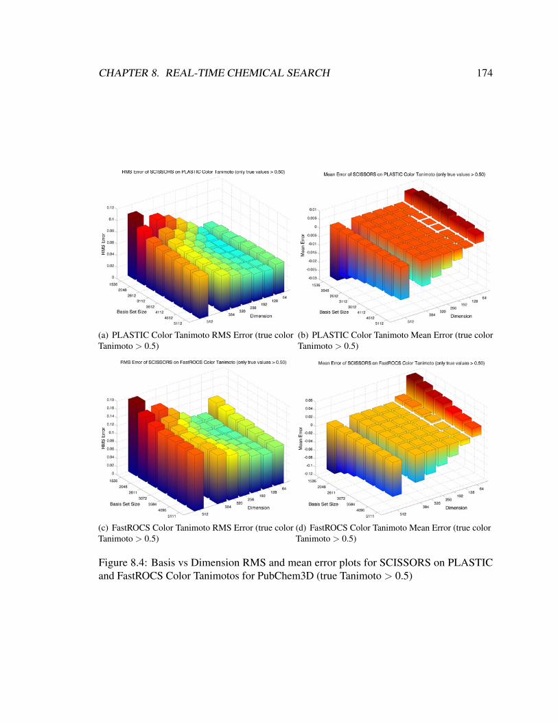
CHAPTER 8. REAL-TIME CHEMICAL SEARCH 174
(a) PLASTIC Color Tanimoto RMS Error (true colorTanimoto > 0.5)
(b) PLASTIC Color Tanimoto Mean Error (true colorTanimoto > 0.5)
(c) FastROCS Color Tanimoto RMS Error (true colorTanimoto > 0.5)
(d) FastROCS Color Tanimoto Mean Error (true colorTanimoto > 0.5)
Figure 8.4: Basis vs Dimension RMS and mean error plots for SCISSORS on PLASTICand FastROCS Color Tanimotos for PubChem3D (true Tanimoto > 0.5)
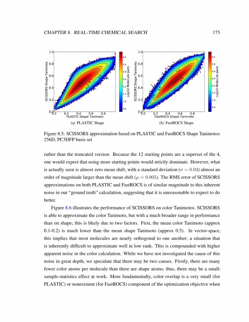
CHAPTER 8. REAL-TIME CHEMICAL SEARCH 175
(a) PLASTIC Shape (b) FastROCS Shape
Figure 8.5: SCISSORS approximation based on PLASTIC and FastROCS Shape Tanimotos:256D, PC3DFP basis set
rather than the truncated version. Because the 12 starting points are a superset of the 4,
one would expect that using more starting points would strictly dominate. However, what
is actually seen is almost zero mean shift, with a standard deviation (σ = 0.03) almost an
order of magnitude larger than the mean shift (µ = 0.005). The RMS error of SCISSORS
approximations on both PLASTIC and FastROCS is of similar magnitude to this inherent
noise in our “ground truth” calculation, suggesting that it is unreasonable to expect to do
better.
Figure 8.6 illustrates the performance of SCISSORS on color Tanimotos. SCISSORS
is able to approximate the color Tanimoto, but with a much broader range in performance
than on shape; this is likely due to two factors. First, the mean color Tanimoto (approx
0.1-0.2) is much lower than the mean shape Tanimoto (approx 0.5). In vector-space,
this implies that most molecules are nearly orthogonal to one another; a situation that
is inherently difficult to approximate well in low rank. This is compounded with higher
apparent noise in the color calculation. While we have not investigated the cause of this
noise in great depth, we speculate that there may be two causes. Firstly, there are many
fewer color atoms per molecule than there are shape atoms; thus, there may be a small-
sample-statistics effect at work. More fundamentally, color overlap is a very small (for
PLASTIC) or nonexistent (for FastROCS) component of the optimization objective when
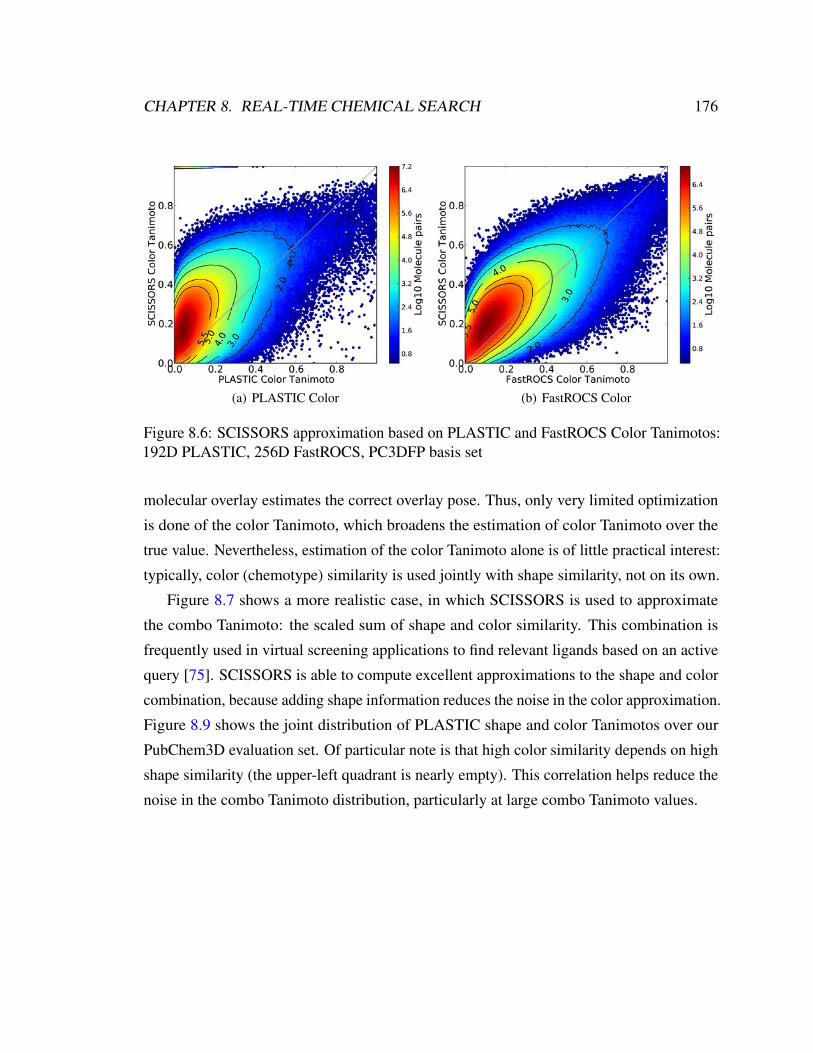
CHAPTER 8. REAL-TIME CHEMICAL SEARCH 176
(a) PLASTIC Color (b) FastROCS Color
Figure 8.6: SCISSORS approximation based on PLASTIC and FastROCS Color Tanimotos:192D PLASTIC, 256D FastROCS, PC3DFP basis set
molecular overlay estimates the correct overlay pose. Thus, only very limited optimization
is done of the color Tanimoto, which broadens the estimation of color Tanimoto over the
true value. Nevertheless, estimation of the color Tanimoto alone is of little practical interest:
typically, color (chemotype) similarity is used jointly with shape similarity, not on its own.
Figure 8.7 shows a more realistic case, in which SCISSORS is used to approximate
the combo Tanimoto: the scaled sum of shape and color similarity. This combination is
frequently used in virtual screening applications to find relevant ligands based on an active
query [75]. SCISSORS is able to compute excellent approximations to the shape and color
combination, because adding shape information reduces the noise in the color approximation.
Figure 8.9 shows the joint distribution of PLASTIC shape and color Tanimotos over our
PubChem3D evaluation set. Of particular note is that high color similarity depends on high
shape similarity (the upper-left quadrant is nearly empty). This correlation helps reduce the
noise in the combo Tanimoto distribution, particularly at large combo Tanimoto values.
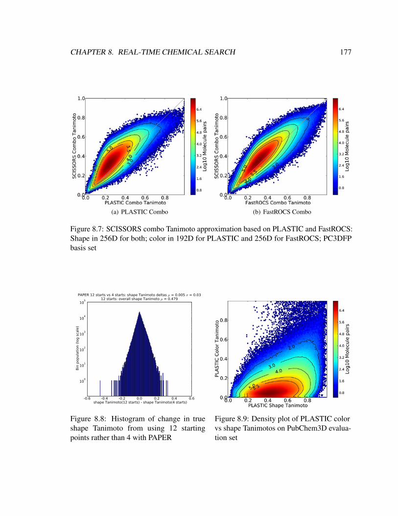
CHAPTER 8. REAL-TIME CHEMICAL SEARCH 177
(a) PLASTIC Combo (b) FastROCS Combo
Figure 8.7: SCISSORS combo Tanimoto approximation based on PLASTIC and FastROCS:Shape in 256D for both; color in 192D for PLASTIC and 256D for FastROCS; PC3DFPbasis set
-0.6 -0.4 -0.2 0.0 0.2 0.4 0.6shape Tanimoto(12 starts) - shape Tanimoto(4 starts)
100
101
102
103
104
105
Bin
popula
tion (
log s
cale
)
PAPER 12 starts vs 4 starts: shape Tanimoto deltas µ = 0.005 σ = 0.0312 starts: overall shape Tanimoto µ = 0.479
Figure 8.8: Histogram of change in trueshape Tanimoto from using 12 startingpoints rather than 4 with PAPER
Figure 8.9: Density plot of PLASTIC colorvs shape Tanimotos on PubChem3D evalua-tion set

CHAPTER 8. REAL-TIME CHEMICAL SEARCH 178
8.8 Results: Throughput
Combining GPU acceleration for direct shape and color Tanimoto calculation with the
SCISSORS approximation algorithm enables real-time search throughput on PubChem-
scale databases. Given precomputed vector representations for the database molecules
(which we have computed for all of PubChem3D), the PLASTIC+SCISSORS combination
can do a full shape and color search for a new query compound (not present in the database)
against the entire database in approximately one second on one server. Performing multiple
queries simultaneously against the same database can further amortize this cost; in the N2
limit of computing all pairwise similarities, we are able to achieve approximately 274,000x
speedup relative to using ROCS to compute all similarities.
Precomputation of the database vectors is a significant, though not prohibitive, expense.
This is dominated by the cost of performing the direct shape and color Tanimoto calculations,
both pairwise between basis molecules, and between library and basis molecules; the number
of Tanimoto calculations required for B basis and L library molecules is described by the
equation:
NumTan =(B)(B − 1)
2+ LB
For even modest library sizes, this is rapidly dominated by the latter term (since the
basis is typically much smaller than the library). For PubChem3D, we must evaluate
approximately 26002/2 + 2600 ∗ 17 × 106 ≈ 44.2 × 10⁹ Tanimotos: approximately one
month of computation on a single NVIDIA GeForce GTX 480 GPU using PLASTIC. The
subsequent linear algebra steps (eigendecomposition of the basis matrix and least-squares
projection of library vectors) are negligible in cost, taking hours on a few CPU cores. At the
chosen dimensionalities, the vector representations fit in under 35GB of storage.
Once the database vectors have been computed, searching based on a new non-database
query proceeds in two steps. First, PLASTIC is used to compute Tanimotos from the
query against the database basis set; at 2,612 basis molecules, this takes under 200ms
on a single GPU. These Tanimotos are then projected into the SCISSORS vector space
(milliseconds or less), and finally vector Tanimotos are computed against the database
vectors. For a single query, the dominant cost in computing these vector Tanimotos is the
time of streaming vectors in from main memory to the CPU. A typical 2010-era server
CHAPTER 8. REAL-TIME CHEMICAL SEARCH 179
able to keep the SCISSORS database in memory will feature approximately 40GB/s of
main memory bandwidth (20GB/s per socket, over two CPU sockets); thus, this phase can
complete in under a second. Indeed, because this ∼ 1-second cost is constant, several query
molecules (or conformers) represented by distinct vectors can be compared at the same time
with essentially no additional slowdown until an arithmetic performance limit is reached.
The particular limit depends on CPU architecture and number of cores, but typical current
servers should be able to handle ten simultaneous queries with no slowdown relative to one.
GPUs can also be used profitably to accelerate the vector-comparison portion of the
SCISSORS search scheme. The most expensive part of the Tanimoto calculation is the dot
product between the two vectors; GPUs are highly efficient at performing this type of dense
linear algebra. However, GPUs typically have much smaller amounts of onboard memory
than would be available to a CPU on a server. Thus, they are not well-suited (in the absence
of multi-GPU parallelism) to performing single-query-vs-database searches. Only small
database pieces could be stored on-GPU at a time, which would constrain the search to the
rate at which database pieces could be moved from main memory across the peripheral bus
to the GPU (∼ 4 GB/s).
GPUs are an excellent choice for larger comparisons, such as N2 pairwise similarity
problems. These applications are able to reuse database vectors more effectively, and are
therefore bound by arithmetic throughput rather than memory bandwidth. The dominant
costs in computing a SCISSORS combo Tanimoto based on the PLASTIC vectors described
here are a 256D and a 192D dot product, which combined require approximately 450
multiply-adds. The NVIDIA GeForce GTX 580, a current high-end GPU, has 512 scalar
processors clocked at 1.544GHz, with each scalar unit able to perform one fused multiply-
add (FMA) per cycle; these specifications imply an upper bound of ∼ 1.8× 10⁹ SCISSORS
dot products per second. Allowing for additional overhead in the computation (memory
loads to cache, division, etc.), even a conservative estimate of 33% efficiency shows that
bulk throughput of 600 million shape+color Tanimotos/second is achievable per-GPU: 4
million times faster than the equivalent computation using ROCS on the CPU. In the case of
full pairwise similarity comparison of PubChem3D, the pairwise vector Tanimotos would
take around 5 days on a single GTX 580. Thus, combining PLASTIC (for library-vs-basis
computations) with SCISSORS on the GPU (to accelerate bulk Tanimoto computations)

CHAPTER 8. REAL-TIME CHEMICAL SEARCH 180
yields a runtime of around 40 GPU-days to compute (17× 106)2 shape and color Tanimotos:
almost 275,000 times speedup relative to the same calculation on a single CPU using
OpenEye ROCS.
8.9 Conclusions
The high-speed chemical search capabilities described in this chapter enable a wide range
of practical applications for 3-D search methods in drug discovery and computational
biochemistry. An interesting direction for drug discovery is the creation of interactive
compound design interfaces, in which chemists can design compounds at a computer and
receive feedback about the presence of similar compounds in a database in real time. In
this application, the reduction in search latency from hours to seconds (or less) enables a
level of interactivity simply impossible with prior methods. Clustering methods are also
important in drug discovery and industrial project management; they are often used, for
example, in managing corporate compound collections and purchases. Compound clustering
by hierarchical agglomerative clustering or Jarvis-Patrick [47] requires the computation
of O(N2) similarities, which is infeasible on million-molecule scale datasets without the
acceleration techniques described here. Additionally, because SCISSORS computes a
vector embedding for each molecule, it enables the use of more-efficient vector clustering
techniques, such as k-means, potentially reducing the computational cost of clustering from
quadratic to linear.
Biochemical machine learning also stands to benefit from such techniques. In particular,
the use of SCISSORS-approximated similarities for large pairwise comparisons allows
rapid assessment of the distribution of similarities in a dataset, and thereby allows accurate
assignment of significance scores (e.g., Z-values) to particular Tanimoto values. These
significance scores (and, indeed, the approximate similarities themselves) can then be used
to induce probabilistic graphical models on chemical data sets. A very simple form of such a
learning method would be a k-nearest-neighbors classifier defined on a large data set, using
the principle of similarity to predict new function. Such methods can be generalized to more
complicated models. For example, thresholding similarities above a certain score (e.g., by
statistical significance) could be used to create a graph with molecules at vertices and edges
CHAPTER 8. REAL-TIME CHEMICAL SEARCH 181
between “significantly similar” molecules. Given an activity label on a training subset of
vertices, this graph could be used to train a Markov random field model of activity. Crucially,
O(N2) similarity calculations are needed to set up the graph structure of such a model, even
if the resultant graph is relatively sparse; the high-speed techniques here described are very
well-suited to such O(N2) problems.
8.10 Acknowledgments
The author thanks Del Lucent (Stanford/CSIRO Molecular and Health Technologies, Mel-
bourne) for contributions to the development of PLASTIC (CPU-side code for parsing color
force fields).

Chapter 9
Conclusion and Future Directions
In the introduction to this dissertation, I argued that the performance of chemical similarity
comparison is a key factor limiting the ability of biochemical machine learning (BML) to
scale to next-generation data sets, and that analysis of these data sets will be critical to the
continued development of computational biochemistry. These computational limitations
occur in both space and time: both our storage capacity and our processing performance are
inadequate to handle the largest current data sets.
Through the course of this dissertation, I have demonstrated that a two-pronged approach
combining hardware acceleration with approximation algorithms is able to solve both the
storage and processing scaling problems for an interesting and industrially-useful class of
chemical similarity measures. Specifically, I have used graphics processing units (GPUs)
to accelerate the evaluation of both two-dimensional (chemical graph-based) and three-
dimensional (shape- and chemotype-based) similarity comparisons by a factor of 30 to
100. I then presented the SCISSORS algorithm, a metric embedding technique that allows
high-quality approximate evaluations of the considered 2D and 3D similarities at effective
rates thousands to millions of times higher than evaluation of the exact similarity function.
This combination can compute similarities faster than precomputed similarities could be
read back from disk, effectively solving the storage problem for large-scale similarity
problems. Analysis of the SCISSORS algorithm leads to bounds on its approximation
performance, based on connections to kernel principal components analysis and the Nystrom
approximation, as well as an analysis of the behavior of kernel approximation in the presence
182
CHAPTER 9. CONCLUSION AND FUTURE DIRECTIONS 183
of inexact kernel evaluation.
The advances presented in this dissertation suggest a number of directions for future
investigation, which I will categorize by subject area: work on new similarity calculation
techniques, research into kernel methods, and applications of this dissertation’s methods in
biochemical machine learning.
9.1 Directions in Chemical Similarity Search
9.1.1 Reducing Noise in Shape Similarity
In Chapter 2 of this work, I applied the increased arithmetic throughput from GPUs to
accelerate the performance (in evaluations/sec) of 3D shape comparison. However, the
results of Chapter 7 suggest an interesting alternative application of these additional FLOP/s.
PAPER follows the original Grant et al. [33] prescription for three-dimensional shape
comparison; in particular, it uses a second-order truncation of the overlap objective function
(considering only pairwise atomic overlaps) and a local optimization scheme to find the
best overlay. However, Chapter 7 demonstrates that these approximations add sufficient
error to the shape-overlap kernel function to impede low-rank approximation efforts. Since
the SCISSORS low-rank approximation is critical to achieving maximum performance on
large-scale similarity comparison it makes sense to tailor the source similarity calculation
for best performance in the approximation by reducing kernel noise.
The extension of shape overlay comparison to higher-order overlaps is a particularly
simple (and thus, appealing) future option. Because the second-order truncation does not
remove doubly-counted regions of space from the overlap volume, it is an overestimator
for the true overlap. Adding higher-order overlap terms would be easily handled with the
color force field interaction matrix used to implement chemotype comparison in PLASTIC,
described in Chapter 8. All order-three overlap functions, in the Gaussian formalism, can
be described as the product of three atom-centered Gaussians. In the Grant and Pickup
2nd-order method, the product of two Gaussians is reduced to a single Gaussian, which has
an analytic integral. Similarly, it should be possible to reduce a 3rd-order interaction to
the product of an atom-centered Gaussian and a “virtual” Gaussian constructed from the

CHAPTER 9. CONCLUSION AND FUTURE DIRECTIONS 184
product of the remaining two atoms’ densities. These virtual Gaussians are thus equivalent
to color/chemotype virtual atoms of a new type: this “shape-pair” type has a negative
interaction with standard shape atoms, and no interaction with other atoms. This general
approach, in which high-order overlaps are reduced to pairwise overlaps between shape
atoms and virtual atoms, with varying weight depending on the sign of the term, can be
generalized to arbitrarily high order (though the number of virtual atoms in a structure will
grow combinatorially quickly).
An alternative way to reduce the noise in shape comparison would be to modify the final
step in the algorithm. As currently described, PAPER/PLASTIC choose the final “winning”
pose from the optimized pool of starting poses by evaluating the (truncated second-order)
objective. This leads to the very small shift in performance seen in Figure 7.1: adding
starting points is almost as likely to hurt the true objective as help it, since the minima of the
true and truncated objectives do not align. Adding a rescoring step, in which each optimized
pose is rescored using the exact scoring function (e.g., by high-resolution quadrature on
the GPU), would restore the desired optimization property that adding starting positions
cannot hurt the final answer. While quadrature may be too expensive for every objective
evaluation during pose optimization, a single rescoring evaluation at the end, particularly
when GPU-accelerated, may still maintain high overall throughput while reducing noise.
9.1.2 Accelerating SCISSORS-based searches
The high dimensionality of SCISSORS vectors is a limiting factor in their search perfor-
mance. In particular, it would be desirable to reduce the memory bandwidth requirements
for SCISSORS-based one-vs-many searches, in which streaming the database vectors from
main memory is the bottleneck. Here, the optimality properties of the kernel PCA projection
underlying SCISSORS may allow significant speedups in the (common) case where only a
few high-scoring hits are desired from a database, rather than a full rank-ordering. Because
dimensions in the SCISSORS projection are sorted in descending order of importance to
the overall similarity, it should be possible to incrementally search a SCISSORS database
by considering low-dimensional subspaces in the SCISSORS space at a time. For example,
given 256-D SCISSORS vectors, it may be possible to do a search on the first 16 dimensions

CHAPTER 9. CONCLUSION AND FUTURE DIRECTIONS 185
alone for the whole database and filter out compounds which are unlikely to appear in the
final result list. Such a hierarchical strategy has the hope of significantly reducing bandwidth
costs at the expense of increased complexity and increased false-positive/negative rate.
9.2 Topics in Kernel Methods
The analysis of low-rank approximation in the presence of noise presented in Chapter
7, while experimentally relevant to the analysis of SCISSORS for shape approximation,
has several limitations. In particular, our perturbation analysis in its current form only
considers zero-mean iid Gaussian noise. The extension of this analysis to other forms of
kernel inexactitude may be of significant interest. In particular, errors in kernel functions
will typically be neither independent nor identically distributed among kernel elements:
one may imagine a dependence on each data point, such that noise terms within a row or
column might be significantly correlated, with distinct distributions per-row or -column.
Additionally, the assumption of normality of the noise, while analytically tractable, is strong.
Using the Central Limit Theorem, it should be possible to demonstrate that our results hold
for a larger class of error distributions. Work examining other distributions without invoking
the CLT may also be useful: in particular, distributions arising from quantization error,
numerical roundoff, and approximate function evaluation (e.g., transcendental functions)
may be of interest in a number of numerical applications.
9.3 Applications in Biochemical Machine Learning
The high-speed similarity techniques described in this dissertation enable a wide range
of potential applications in biochemical machine learning. These applications benefit
from three attributes of the described methods: fast one-vs-many search using GPUs or
precalculated SCISSORS databases, accelerated many-vs-many search using SCISSORS,
and the translation of non-vectorial molecular data into a vector space.

CHAPTER 9. CONCLUSION AND FUTURE DIRECTIONS 186
9.3.1 Fast One-vs-Many Search
As I argued in Chapter 8, the ability to perform similarity queries on million-molecule scale
databases with turnaround time in seconds enables new workflows in medicinal chemistry.
Computer-aided design tools in medicinal chemistry are often used as “idea generation”
techniques, in which new chemical proposals are shown to bench chemists in response to
structural information or previous compounds in a series. However, the slow speed of prior
search methods restricted the application of 3D-similarity-based proposals to batch mode
processing. The ability to return results in seconds makes possible an interactive workflow,
in which chemists could sketch out a desired compound and in real time see compounds of
similar shape and functionality from a database, without waiting for a slow batch query.
9.3.2 Fast Many-vs-Many Search
The conclusion to Chapter 8 describes an application of GPU+SCISSORS accelerated
similarity search to build a probabilistic graphical model on chemical space by connecting
highly-related compounds in a Markov graphical model. Another interesting application of
many-vs-many search is to directly predict protein binding partners of given molecules by
shape comparison.
It would be possible to construct a space-filling model of a protein binding pocket
(possibly with virtual color atoms representing desirable chemotypes at particular sites in the
binding cavity), and then compare these “negative images” directly with compounds. Such
a problem, given the thousands of available protein structures and millions of compounds
currently known, requires fast pairwise comparison in order to be tractable. The scale of the
problem is dramatically expanded by considering protein flexibility. In principle, molecular
dynamics or Monte Carlo simulations could be used to sample the accessible conformational
space of a protein binding pocket; each accessible conformational state would then be
modeled by a different space-filling model, perhaps growing the problem by a factor of 10
to 100.

CHAPTER 9. CONCLUSION AND FUTURE DIRECTIONS 187
9.3.3 Projecting Molecules into Vector Spaces
Because molecules are not naturally interpreted as elements of a vector space, many tech-
niques from machine learning (usually defined on vectorial data) are not easily applied to
biochemistry. The use of an appropriate set of features to represent molecules as vectors is
thus critical for machine learning. However, in some cases, it is simpler to define a similarity
or distance function between molecules than it is to define a set of features to reproduce that
similarity. For example, minimum-distance field similarities such as electrostatic and shape
similarity are easily defined algorithmically, but defy a simple feature-space definition be-
cause of their invariance to rotation and translation of the molecules in question. SCISSORS
provides a method to compute an optimal feature-space projection for molecules based on
a similarity score, under the assumptions that the feature space is adequately sampled by
a small set of landmark molecules and the eigenspectrum of the similarity function falls
off rapidly. Thus, SCISSORS enables the application of vector-based machine learning
methods to chemical data by computing vector features of molecules based on particular
chemical similarities. An especially interesting application of this vector-space projection
would be to learn SCISSORS features for a variety of similarity functions based on different
chemical data (e.g., shape, chemotype, electrostatics, chemical graph, etc.) and then use
feature selection or metric learning to train a new similarity measure fusing the relevant
features of each component similarity method.

Bibliography
[1] ACHLIOPTAS, D. Random matrices in data analysis. In Proc. 15th European Conf. on
Machine Learning (2004), pp. 1–8.
[2] ACHLIOPTAS, D., MCSHERRY, F., AND SCHOLKOPF, B. Sampling techniques for
kernel methods. In Annual Advances in Neural Information Processing Systems 14:
Proceedings of the 2001 Conference (2001), vol. 14, pp. 335–342.
[3] AHO, A. V., AND CORASICK, M. J. Efficient string matching: an aid to bibliographic
search. Commun. ACM 18, 6 (June 1975), 333–340.
[4] ALBISTON, A. L., MORTON, C. J., NG, H. L., PHAM, V., YEATMAN, H. R.,
YE, S., FERNANDO, R. N., DE BUNDEL, D., ASCHER, D. B., MENDELSOHN, F.
A. O., PARKER, M. W., AND CHAI, S. Y. Identification and characterization of a
new cognitive enhancer based on inhibition of insulin-regulated aminopeptidase. The
FASEB Journal 22, 12 (Dec. 2008), 4209–4217.
[5] BALLESTER, P. J., AND RICHARDS, W. G. Ultrafast shape recognition to search
compound databases for similar molecular shapes. J. Comput. Chem. 28, 10 (July
2007), 1711–1723.
[6] BATSANOV, S. S. Van der Waals radii of elements. Inorg Mat 37, 9 (2001), 871–885.
[7] BENGIO, Y., DELALLEAU, O., ROUX, N. L., PAIEMENT, J.-F., VINCENT, P., AND
OUIMET, M. Learning eigenfunctions links spectral embedding and kernel PCA.
Neural Comput. 16, 10 (October 2004), 2197–2219.
188

BIBLIOGRAPHY 189
[8] BLUM, L. C., AND REYMOND, J.-L. 970 million druglike small molecules for virtual
screening in the chemical universe database GDB-13. J. Am. Chem. Soc. 131, 25 (July
2009), 8732–8733.
[9] BOHACEK, R. S., MCMARTIN, C., AND GUIDA, W. C. The art and practice of
structure-based drug design: A molecular modeling perspective. Med. Res. Rev. 16, 1
(1996), 3–50.
[10] BOLTON, E. E., KIM, S., AND BRYANT, S. H. PubChem3D: Conformer generation.
J. Cheminformatics 3, 1 (Mar. 2011).
[11] BOLTON, E. E., KIM, S., AND BRYANT, S. H. PubChem3D: Diversity of shape. J.
Cheminformatics 3, 1 (Mar. 2011).
[12] BONDI, A. van der Waals volumes and radii. J. Phys. Chem. 68, 3 (March 1964),
441–451.
[13] BOSER, B. E., GUYON, I. M., AND VAPNIK, V. N. A training algorithm for optimal
margin classifiers. In Proceedings of the 5th Annual Workshop on Computational
Learning Theory (New York, NY, USA, 1992), COLT ’92, ACM, pp. 144–152.
[14] BRAUN, M. L., BUHMANN, J., AND MUELLER, K.-R. Denoising and dimension
reduction in feature space. In Annual Advances in Neural Information Processing
Systems 19: Proceedings of the 2006 Conference (2007), vol. 19.
[15] BUTINA, D. Unsupervised data base clustering based on Daylight’s fingerprint and
Tanimoto similarity: A fast and automated way to cluster small and large data sets. J.
Chem. Inf. Comput. Sci. 39, 4 (July 1999), 747–750.
[16] CARHART, R. E., SMITH, D. H., AND VENKATARAGHAVAN, R. Atom pairs as
molecular features in structure-activity studies: definition and applications. J. Chem.
Inf. Comput. Sci. 25, 2 (May 1985), 64–73.
[17] CHARIFSON, P. S., Ed. Practical Application of Computer-Aided Drug Design, 1 ed.
Marcel Dekker, New York, July 1997.

BIBLIOGRAPHY 190
[18] CHEESERIGHT, T., MACKEY, M., ROSE, S., AND VINTER, A. Molecular field
extrema as descriptors of biological activity: Definition and validation. J. Chem. Inf.
Model. 46, 2 (Mar. 2006), 665–676.
[19] CHODERA, J. D., MOBLEY, D. L., SHIRTS, M. R., DIXON, R. W., BRANSON, K.,
AND PANDE, V. S. Alchemical free energy methods for drug discovery: progress and
challenges. Curr. Opin. Struct. Biol. 21, 2 (Apr. 2011), 150–160.
[20] CLARK, R. D., AND WEBSTER-CLARK, D. J. Managing bias in ROC curves. J.
Comput. Aided Mol. Des. (February 2008).
[21] CONNOLLY, M. L. Computation of molecular volume. J. Am. Chem. Soc. 107, 5
(1985), 1118–1124.
[22] COX, T. F., AND COX, M. A. A. Multidimensional Scaling. Chapman & Hall,
London, January 1994.
[23] DENG, Y., AND ROUX, B. Computation of binding free energy with molecular
dynamics and grand canonical Monte Carlo simulations. The Journal of Chemical
Physics 128, 11 (2008), 115103+.
[24] DRINEAS, P., AND MAHONEY, M. W. On the Nystrom method for approximating a
Gram matrix for improved kernel-based learning. J. Mach. Learn. Res. 6 (2005).
[25] DURANT, J. L., LELAND, B. A., HENRY, D. R., AND NOURSE, J. G. Reoptimization
of MDL keys for use in drug discovery. J. Chem. Inf. Comput. Sci. 42, 6 (November
2002), 1273–1280.
[26] FERRARA, P., GOHLKE, H., PRICE, D. J., KLEBE, G., AND BROOKS, C. L. Assess-
ing Scoring Functions for Protein-Ligand Interactions. Journal of Medicinal Chemistry
47, 12 (June 2004), 3032–3047.
[27] FONTAINE, F., BOLTON, E., BORODINA, Y., AND BRYANT, S. H. Fast 3D shape
screening of large chemical databases through alignment-recycling. Chem. Cent. J. 1
(2007), 12.

BIBLIOGRAPHY 191
[28] FRIEDRICHS, M. S., EASTMAN, P., VAIDYANATHAN, V., HOUSTON, M., LEGRAND,
S., BEBERG, A. L., ENSIGN, D. L., BRUNS, C. M., AND PANDE, V. S. Accelerating
molecular dynamic simulation on graphics processing units. J. Comput. Chem. 30, 6
(2009), 864–872.
[29] GAMO, F.-J., SANZ, L. M., VIDAL, J., DE COZAR, C., ALVAREZ, E., LAVANDERA,
J.-L., VANDERWALL, D. E., GREEN, D. V. S., KUMAR, V., HASAN, S., BROWN,
J. R., PEISHOFF, C. E., CARDON, L. R., AND GARCIA-BUSTOS, J. F. Thousands
of chemical starting points for antimalarial lead identification. Nature 465, 7296 (May
2010), 305–310.
[30] GASIOROWICZ, S. Quantum Physics. John Wiley and Sons, New York, 1974.
[31] GOLUB, G. H., AND VAN LOAN, C. F. Matrix Computations, 3rd ed. The Johns
Hopkins University Press, Baltimore, October 1996.
[32] GOTO, K., AND VAN DE GEIJN, R. High-performance implementation of the level-3
BLAS. ACM Trans. Math. Softw. 35, 1 (2008), 1–14.
[33] GRANT, J. A., GALLARDO, M. A., AND PICKUP, B. T. A fast method of molecular
shape comparison: A simple application of a Gaussian description of molecular shape.
J. Comp. Chem. 17, 14 (1996), 1653–1666.
[34] GRANT, J. A., HAIGH, J. A., PICKUP, B. T., NICHOLLS, A., AND SAYLE, R. A.
Lingos, finite state machines, and fast similarity searching. J. Chem. Inf. Model. 46, 5
(September 2006), 1912–1918.
[35] GRANT, J. A., AND PICKUP, B. T. A Gaussian description of molecular shape. J.
Phys. Chem. 99, 11 (1995).
[36] GRIEWANK, A. O., MARKEY, B. R., AND EVANS, D. J. Singularity-free static lattice
energy minimization. J. Chem. Phys. 71, 8 (1979), 3449–3454.

BIBLIOGRAPHY 192
[37] GUNDERSEN, E., FAN, K., HAAS, K., HURYN, D., JACOBSEN, J. S., KREFT, A.,
MARTONE, R., MAYER, S., SONNENBERG-REINES, J., AND SUN, S. Molecular-
modeling based design, synthesis, and activity of substituted piperidines as gamma-
secretase inhibitors. Bioorg & Med Chem Lett 15, 7 (April 2005), 1891–1894.
[38] HAIGH, J. A., PICKUP, B. T., GRANT, J. A., AND NICHOLLS, A. Small molecule
shape-fingerprints. J. Chem. Inf. Model 45, 3 (May 2005), 673–684.
[39] HAQUE, I. S., AND PANDE, V. S. PAPER — accelerating parallel evaluations of
ROCS. J. Comput. Chem. 31, 1 (2009), 117–132.
[40] HAQUE, I. S., AND PANDE, V. S. SCISSORS: A linear-algebraical technique to
rapidly approximate chemical similarities. J. Chem. Inf. Model. 50, 6 (June 2010),
1075–1088.
[41] HAQUE, I. S., AND PANDE, V. S. Large-Scale chemical informatics on GPUs. In
GPU Computing Gems: Emerald Edition (Feb. 2011), W.-m. W. Hwu, Ed., Morgan
Kaufmann.
[42] HAQUE, I. S., PANDE, V. S., AND WALTERS, W. P. SIML: A fast SIMD algorithm
for calculating LINGO chemical similarities on GPUs and CPUs. J. Chem. Inf. Model.
50, 4 (Apr. 2010), 560–564.
[43] HUANG, N., KALYANARAMAN, C., IRWIN, J. J., AND JACOBSON, M. P. Physics-
Based Scoring of Protein-Ligand Complexes: Enrichment of Known Inhibitors in
Large-Scale Virtual Screening. J. Chem. Inf. Model. 46, 1 (Jan. 2006), 243–253.
[44] HUANG, N., SHOICHET, B. K., AND IRWIN, J. J. Benchmarking sets for molecular
docking. J. Med. Chem. 49, 23 (October 2006), 6789–6801.
[45] IRWIN, J. J., AND SHOICHET, B. K. ZINC — a free database of commercially
available compounds for virtual screening. J. Chem. Inf. Model. 45, 1 (2005), 177–182.
[46] JAIN, A. N. Ligand-based structural hypotheses for virtual screening. J. Med. Chem.
47, 4 (February 2004), 947–961.

BIBLIOGRAPHY 193
[47] JARVIS, R. A., AND PATRICK, E. A. Clustering using a similarity measure based
on shared near neighbors. IEEE Transactions on Computers C-22, 11 (Nov. 1973),
1025–1034.
[48] JENKINS, J. L., GLICK, M., AND DAVIES, J. W. A 3D similarity method for scaffold
hopping from known drugs or natural ligands to new chemotypes. J. Med. Chem. 47,
25 (Dec. 2004), 6144–6159.
[49] JENKINS, O. C. Localization from pairwise distance relationships using kernel PCA.
Tech. Rep. CRES-03-010, Los Angeles, USA, 2003.
[50] JORGENSEN, W. L. Efficient Drug Lead Discovery and Optimization. Accounts Chem.
Res. 42, 6 (June 2009), 724–733.
[51] KEARSLEY, S. K. An algorithm for the simultaneous superposition of a structural
series. J. Comp. Chem. 11, 10 (1990), 1187–1192.
[52] KLEPEIS, J. L., LINDORFF-LARSEN, K., DROR, R. O., AND SHAW, D. E. Long-
timescale molecular dynamics simulations of protein structure and function. Curr.
Opin. Struct. Biol. 19, 2 (Apr. 2009), 120–127.
[53] LAUB, J., ROTH, V., BUHMANN, J. M., AND MULLER, K. R. On the information
and representation of non-Euclidean pairwise data. Pattern Recogn. 39 (Oct. 2006),
1815–1826.
[54] LI, H., YAP, C. W., UNG, C. Y., XUE, Y., CAO, Z. W., AND CHEN, Y. Z. Effect of
selection of molecular descriptors on the prediction of blood-brain barrier penetrating
and nonpenetrating agents by statistical learning methods. J. Chem. Inf. Model. 45, 5
(September 2005), 1376–1384.
[55] LINDHOLM, E., NICKOLLS, J., OBERMAN, S., AND MONTRYM, J. NVIDIA Tesla:
A unified graphics and computing architecture. IEEE Micro 28, 2 (2008), 39–55.
[56] LODHI, H., SAUNDERS, C., SHAWE-TAYLOR, J., CRISTIANINI, N., AND WATKINS,
C. Text classification using string kernels. J. Mach. Learn. Res. 2 (Feb. 2002),
419–444.

BIBLIOGRAPHY 194
[57] MARTIN, E. J., BLANEY, J. M., SIANI, M. A., SPELLMEYER, D. C., WONG,
A. K., AND MOOS, W. H. Measuring diversity: Experimental design of combinatorial
libraries for drug discovery. J. Med. Chem. 38, 9 (April 1995), 1431–1436.
[58] MILLER, M. D., SHERIDAN, R. P., AND KEARSLEY, S. K. SQ: A program for
rapidly producing pharmacophorically relevent molecular superpositions. J. Med.
Chem. 42, 9 (May 1999), 1505–1514.
[59] MUCHMORE, S. W., SOUERS, A. J., AND AKRITOPOULOU-ZANZE, I. The use of
three-dimensional shape and electrostatic similarity searching in the identification of a
melanin-concentrating hormone receptor 1 antagonist. Chem. Biol. Drug Des. 67, 2
(February 2006), 174–176.
[60] NICHOLLS, A. Method for determining a shape space for a set of molecules using
minimal metric distances. U.S. Patent 7,110,888 (September 2006).
[61] NICHOLLS, A., AND GRANT, J. A. Molecular shape and electrostatics in the encoding
of relevant chemical information. J. Comput.-Aided Mol. Des. 19, 9 (September 2005),
661–686.
[62] NICHOLLS, A., MACCUISH, N., AND MACCUISH, J. Variable selection and model
validation of 2D and 3D molecular descriptors. J. Comput.-Aided Mol. Des. 18, 7 (July
2004), 451.
[63] NICKOLLS, J., BUCK, I., GARLAND, M., AND SKADRON, K. Scalable parallel
programming with CUDA. ACM Queue 6, 2 (2008), 40–53.
[64] NIKOLOVA, N., AND JAWORSKA, J. Approaches to measure chemical similarity - a
review. QSAR & Combin. Sci. 22, 9-10 (January 2003), 1006–1026.
[65] NVIDIA. NVIDIA CUDA Programming Guide 2.0. NVIDIA, 2008.
[66] ODONE, F., BARLA, A., AND VERRI, A. Building kernels from binary strings for
image matching. IEEE Trans. Image Proc. 14, 2 (Feb. 2005), 169–180.

BIBLIOGRAPHY 195
[67] OMEGA IN OPENEYE PYTHON TOOLKITS, VERSION 1.5.1-1. OpenEye Scientific
Software, Inc., Santa Fe, NM, USA, www.eyesopen.com. (2007).
[68] PEKALSKA, E. M. Dissimilarity representations in pattern recognition. Concepts,
theory and applications. PhD thesis, Wroclaw University, Wroclaw, Poland, January
2005.
[69] PONDER, J. W., WU, C., REN, P., PANDE, V. S., CHODERA, J. D., SCHNIEDERS,
M. J., HAQUE, I., MOBLEY, D. L., LAMBRECHT, D. S., DISTASIO, R. A., HEAD-
GORDON, M., CLARK, G. N. I., JOHNSON, M. E., AND HEAD-GORDON, T. Current
Status of the AMOEBA Polarizable Force Field. J. Phys. Chem. B 114, 8 (Mar. 2010),
2549–2564.
[70] PRESS, W. H., FLANNERY, B. P., TEUKOLSKY, S. A., AND VETTERLING, W. T.
Numerical Recipes in C : The Art of Scientific Computing. Cambridge University Press,
October 1992.
[71] RAGHAVENDRA, A. S., AND MAGGIORA, G. M. Molecular basis sets — a general
similarity-based approach for representing chemical spaces. J. Chem. Inf. Model. 47, 4
(July 2007), 1328–1340.
[72] REFSGAARD, H. H., JENSEN, B. F., BROCKHOFF, P. B., PADKJAER, S. B., GULD-
BRANDT, M., AND CHRISTENSEN, M. S. In silico prediction of membrane perme-
ability from calculated molecular parameters. J. Med. Chem. 48 (Feb 2005), 805–811.
[73] ROCS. OpenEye Scientific Software, Inc., Santa Fe, NM, USA, www.eyesopen.com
(2008).
[74] ROGERS, D., AND HAHN, M. Extended-connectivity fingerprints. J. Chem. Inf.
Model. 50 (May 2010), 742–754.
[75] RUSH, T. S., GRANT, J. A., MOSYAK, L., AND NICHOLLS, A. A shape-based 3-d
scaffold hopping method and its application to a bacterial protein-protein interaction.
J. Med. Chem. 48, 5 (March 2005), 1489–1495.

BIBLIOGRAPHY 196
[76] SCHNEIDER, G., NEIDHART, W., GILLER, T., AND SCHMID, G. ”Scaffold-Hopping”
by topological pharmacophore search: a contribution to virtual screening. Angewandte
Chemie (Intl. ed. in English) 38, 19 (Oct. 1999), 2894–2896.
[77] SCHOLKOPF, B., SMOLA, A., AND MULLER, K.-R. Nonlinear component analysis
as a kernel eigenvalue problem. Tech. Rep. 44, Tuebingen, Germany, December 1996.
[78] SCHOLKOPF, B., SMOLA, A., AND MULLER, K.-R. Nonlinear component analysis
as a kernel eigenvalue problem. Neural Comput. 10, 5 (July 1998), 1299–1319.
[79] SHAWE-TAYLOR, J., WILLIAMS, C. K. I., CRISTIANINI, N., AND KANDOLA, J.
On the eigenspectrum of the Gram matrix and the generalization error of kernel-PCA.
IEEE Trans. Info. Theory 51, 7 (July 2005), 2510–2522.
[80] SHIRTS, M., MOBLEY, D., AND CHODERA, J. Alchemical Free Energy Calculations:
Ready for Prime Time? Annual Reports Comput. Chem. 3 (2007), 41–59.
[81] STONE, J. E., PHILLIPS, J. C., FREDDOLINO, P. L., HARDY, D. J., TRABUCO,
L. G., AND SCHULTEN, K. Accelerating molecular modeling applications with
graphics processors. J. Comput. Chem. 28, 16 (September 2007), 2618–2640.
[82] SUN, D., CHUAQUI, C., DENG, Z., BOWES, S., CHIN, D., SINGH, J., CULLEN,
P., HANKINS, G., LEE, W.-C., DONNELLY, J., FRIEDMAN, J., AND JOSIAH, S. A
kinase-focused compound collection: Compilation and screening strategy. Chem Biol
& Drug Des 67, 6 (June 2006), 385–394.
[83] TALWALKAR, A. Matrix Approximation for Large-scale Learning. PhD thesis,
Courant Institute of Mathematical Sciences, New York University, New York, NY,
May 2010.
[84] TANAKA, N., OHNO, K., NIIMI, T., MORITOMO, A., MORI, K., AND ORITA, M.
Small-world phenomena in chemical library networks: Application to fragment-based
drug discovery. J. Chem. Inf. Model. 12, 49 (2009), 2677–2686.

BIBLIOGRAPHY 197
[85] VIDAL, D., THORMANN, M., AND PONS, M. LINGO, an efficient holographic text
based method to calculate biophysical properties and intermolecular similarities. J.
Chem. Inf. Model. 45, 2 (March 2005), 386–393.
[86] WASSON, S. Nvidia’s GeForce GTX 280 graphics processor. The Tech Report.
(Accessed 1 Jul 2008).
[87] WILLIAMS, C., AND SEEGER, M. Using the Nystrom method to speed up kernel
machines. In Advances in Neural Information Processing Systems 13 (2001), vol. 13,
pp. 682–688.
[88] WILLIAMS, C. K. I. On a connection between kernel pca and metric multidimensional
scaling. Mach. Learn. 46, 1-3 (January 2002), 11–19.
[89] ZAUHAR, R. J., MOYNA, G., TIAN, L., LI, Z., AND WELSH, W. J. Shape signatures:
a new approach to computer-aided ligand- and receptor-based drug design. J. Med.
Chem. 46, 26 (December 2003), 5674–5690.