AC Power Flows and their Derivatives using …AC Power Flows and their Derivatives using Complex Matrix Notation and Cartesian Coordinate Voltages Baljinnyam Sereeter Ray D. Zimmerman

AC Power Flows and their Derivatives usingComplex Matrix Notation and Cartesian

Coordinate Voltages

Baljinnyam Sereeter Ray D. Zimmerman

April 2, 2018∗

Matpower Technical Note 4

c© 2008, 2010, 2011, 2017, 2018 Power Systems Engineering Research Center (Pserc)

All Rights Reserved

∗Revision 2 – June 20, 2019. See Section 8 for revision history details.

CONTENTS CONTENTS

Contents

1 Notation 4

2 Introduction 5

3 Voltages 63.1 Bus Voltages . . . . . . . . . . . . . . . . . . . . . . . . . . . . . . . 6

3.1.1 First Derivatives . . . . . . . . . . . . . . . . . . . . . . . . . 73.1.2 Second Derivatives . . . . . . . . . . . . . . . . . . . . . . . . 7

3.2 Branch Voltages . . . . . . . . . . . . . . . . . . . . . . . . . . . . . . 83.2.1 First Derivatives . . . . . . . . . . . . . . . . . . . . . . . . . 9

3.3 Reference Bus Voltage Angles . . . . . . . . . . . . . . . . . . . . . . 93.3.1 First Derivatives . . . . . . . . . . . . . . . . . . . . . . . . . 93.3.2 Second Derivatives . . . . . . . . . . . . . . . . . . . . . . . . 9

3.4 Bus Voltage Magnitude Limits . . . . . . . . . . . . . . . . . . . . . . 103.4.1 First Derivatives . . . . . . . . . . . . . . . . . . . . . . . . . 103.4.2 Second Derivatives . . . . . . . . . . . . . . . . . . . . . . . . 10

3.5 Branch Angle Difference Limits . . . . . . . . . . . . . . . . . . . . . 113.5.1 First Derivatives . . . . . . . . . . . . . . . . . . . . . . . . . 113.5.2 Second Derivatives . . . . . . . . . . . . . . . . . . . . . . . . 11

4 Bus Injections 124.1 Complex Current Injections . . . . . . . . . . . . . . . . . . . . . . . 12


4.2 Complex Power Injections . . . . . . . . . . . . . . . . . . . . . . . . 174.2.1 First Derivatives . . . . . . . . . . . . . . . . . . . . . . . . . 184.2.2 Second Derivatives . . . . . . . . . . . . . . . . . . . . . . . . 18

5 Branch Flows 205.1 Complex Currents . . . . . . . . . . . . . . . . . . . . . . . . . . . . . 20


5.2 Complex Power Flows . . . . . . . . . . . . . . . . . . . . . . . . . . 205.2.1 First Derivatives . . . . . . . . . . . . . . . . . . . . . . . . . 215.2.2 Second Derivatives . . . . . . . . . . . . . . . . . . . . . . . . 21

5.3 Squared Current Magnitudes . . . . . . . . . . . . . . . . . . . . . . . 235.4 Squared Apparent Power Magnitudes . . . . . . . . . . . . . . . . . . 23

2

CONTENTS CONTENTS

5.5 Squared Real Power Magnitudes . . . . . . . . . . . . . . . . . . . . . 23

6 Generalized AC OPF Costs 23

7 Lagrangian of the AC OPF 247.1 Nodal Current Balance . . . . . . . . . . . . . . . . . . . . . . . . . . 25


7.2 Nodal Power Balance . . . . . . . . . . . . . . . . . . . . . . . . . . . 277.2.1 First Derivatives . . . . . . . . . . . . . . . . . . . . . . . . . 277.2.2 Second Derivatives . . . . . . . . . . . . . . . . . . . . . . . . 27

8 Revision History 29

Appendix A Scalar Polar Coordinate Derivatives 30A.1 First Derivatives . . . . . . . . . . . . . . . . . . . . . . . . . . . . . 30A.2 Second Derivatives . . . . . . . . . . . . . . . . . . . . . . . . . . . . 31

References 32

3

1 NOTATION

1 Notation

nb, ng, nl, nr number of buses, generators, branches, reference buses, respectively

ui, wi real and imaginary parts of bus voltage at bus i

|vi|, θi bus voltage magnitude and angle at bus i

vi complex bus voltage at bus i, that is |vi|ejθi or ui + jwi

U,W nb × 1 vectors of real and imaginary parts of bus voltage

V ,Θ nb × 1 vectors of bus voltage magnitudes and angles

V nb × 1 vector of complex bus voltages vi, U + jW

Ibus nb × 1 vector of complex bus current injections

If , I t nl × 1 vectors of complex branch current injections, from and to ends

Sbus nb × 1 vector of complex bus power injections

Sf , St nl × 1 vectors of complex branch power flows, from and to ends

Sg ng × 1 vector of generator complex power injections

P,Q real and reactive power flows/injections, S = P + jQ

M,N real and imaginary parts of current flows/injections, I = M + jN

Ybus nb × nb system bus admittance matrix

Yf , Yt nl × nb system branch admittance matrices, from and to ends

Cg nb × ng generator connection matrix(i, j)th element is 1 if generator j is located at bus i, 0 otherwise

Cf , Ct nl × nb branch connection matrices, from and to ends,(i, j)th element is 1 if from end, or to end, respectively, of branch i isconnected to bus j, 0 otherwise

Cref nr × nb reference bus indicator matrix(i, j)th element is 1 if bus j is ith reference bus, 0 otherwise

[A] diagonal matrix with vector A on the diagonal

AT (non-conjugate) transpose of matrix A

A∗ complex conjugate of A

Ab matrix exponent for matrix A, or element-wise exponent for vector A

1n, [1n] n× 1 vector of all ones, n× n identity matrix

0 appropriately-sized vector or matrix of all zeros

4

2 INTRODUCTION

2 Introduction

This document is a companion to Matpower Technical Note 2 [1] and MatpowerTechnical Note 3 [2]. The purpose of these documents is to show how the AC powerbalance and flow equations used in power flow and optimal power flow computa-tions can be expressed in terms of complex matrices, and how their first and secondderivatives can be computed efficiently using complex sparse matrix manipulations.The relevant code in Matpower [3–5] is based on the formulas found in these threenotes.

Matpower Technical Note 2 presents a standard formulation based on complexpower flows and nodal power balances using a polar representation of bus voltages,Matpower Technical Note 3 adds the formulas needed for nodal current balances,and this note presents versions of both based on a cartesian coordinate representationof bus voltages.

We will be looking at complex functions of the real valued vector

X =

UWPgQg

. (1)

For a complex scalar function f : Rn → C of a real vector X =[x1 x2 · · · xn

]T,

we use the following notation for the first derivatives (transpose of the gradient)

fX =∂f

∂X=[

∂f∂x1

∂f∂x2

· · · ∂f∂xn

]. (2)

The matrix of second partial derivatives, the Hessian of f , is

fXX =∂2f

∂X2=

∂

∂X

(∂f

∂X

)T

=

∂2f∂x21

· · · ∂2f∂x1∂xn

.... . .

...∂2f

∂xn∂x1· · · ∂2f

∂x2n

. (3)

For a complex vector function F : Rn → Cm of a vector X, where

F (X) =[f1(X) f2(X) · · · fm(X)

]T, (4)

the first derivatives form the Jacobian matrix, where row i is the transpose of thegradient of fi.

FX =∂F

∂X=

∂f1∂x1

· · · ∂f1∂xn

.... . .

...∂fm∂x1

· · · ∂fm∂xn

(5)

5

https://matpower.org/docs/TN2-OPF-Derivatives.pdf

https://matpower.org/docs/TN3-More-OPF-Derivatives.pdf




3 VOLTAGES

In these derivations, the full 3-dimensional set of second partial derivatives of F willnot be computed. Instead a matrix of partial derivatives will be formed by computingthe Jacobian of the vector function obtained by multiplying the transpose of theJacobian of F by a constant vector λ, using the following notation.

FXX(α) =

(∂

∂X

(FX

Tλ))∣∣∣∣

λ=α

(6)

Just to clarify the notation, if Y and Z are subvectors of X, then

FY Z(α) =

(∂

∂Z

(FY

Tλ))∣∣∣∣

λ=α

. (7)

One common operation encountered in these derivations is the element-wise mul-tiplication of a vector A by a vector B to form a new vector C of the same dimension,which can be expressed in either of the following forms

C = [A]B = [B]A (8)

It is useful to note that the derivative of such a vector can be calculated by the chainrule as

CX =∂C

∂X= [A]

∂B

∂X+ [B]

∂A

∂X= [A]BX + [B]AX (9)

3 Voltages

3.1 Bus Voltages

V is the nb×1 vector of complex bus voltages. The element for bus i is vi = ui+jwi.U and W are the vectors of real and imaginary parts of the bus voltages. Consideralso the vector of inverses of bus voltages 1

vi, denoted by Λ. Note that

1

vi=

1

ui + jwi=ui − jwiu2i + w2

i

=vi∗

|vi|2(10)

Λ = V −1 = [V ]−2 V ∗ (11)

Θ = tan−1([U ]−1W

)(12)

V =(U2 +W 2

) 12 (13)

6

3.1 Bus Voltages 3 VOLTAGES

3.1.1 First Derivatives

VU =∂V

∂U= [1nb

] (14)

VW =∂V

∂W= j [1nb

] (15)

ΛU =∂Λ

∂U= − [Λ]2 (16)

ΛW =∂Λ

∂W= −j [Λ]2 (17)

The following could also be useful for implementing certain constraints on volt-age magnitude or angles. For the derivations, see the scalar versions found in Ap-pendix A.

ΘU =∂Θ

∂U= − [V ]−2 [W ] (18)

ΘW =∂Θ

∂W= [V ]−2 [U ] (19)

VU =∂V∂U

= [V ]−1 [U ] (20)

VW =∂V∂W

= [V ]−1 [W ] (21)

3.1.2 Second Derivatives

For the derivations, see the scalar versions found in Appendix A.

ΘUU(λ) =∂

∂U

(ΘU

Tλ)

(22)

= 2 [λ] [V ]−4 [U ] [W ] (23)

ΘUW (λ) =∂

∂W

(ΘU

Tλ)

(24)

7

3.2 Branch Voltages 3 VOLTAGES

= [λ] [V ]−4 ([W ]2 − [U ]2)

(25)

ΘWU(λ) =∂

∂U

(ΘW

Tλ)

(26)

= [λ] [V ]−4 ([W ]2 − [U ]2)

(27)

ΘWW (λ) =∂

∂W

(ΘW

Tλ)

(28)

= −2 [λ] [V ]−4 [U ] [W ] (29)

VUU(λ) =∂

∂U

(VUTλ

)(30)

= [λ] [V ]−3 [W ]2 (31)

VUW (λ) =∂

∂W

(VUTλ

)(32)

= − [λ] [V ]−3 [U ] [W ] (33)

VWU(λ) =∂

∂U

(VWTλ

)(34)

= − [λ] [V ]−3 [U ] [W ] (35)

VWW (λ) =∂

∂W

(VWTλ

)(36)

= [λ] [V ]−3 [U ]2 (37)

3.2 Branch Voltages

The nl × 1 vectors of complex voltages at the from and to ends of all branches are,respectively

Vf = CfV (38)

Vt = CtV (39)

8

3.3 Reference Bus Voltage Angles 3 VOLTAGES


∂Vf∂U

= Cf∂V

∂U= Cf (40)

∂Vf∂W

= Cf∂V

∂W= jCf (41)

3.3 Reference Bus Voltage Angles

The nr × 1 vector of complex voltages at reference buses is

Vref = CrefV (42)

The equality constraint on voltage angles at reference buses is

Gref(X) = CrefΘ−Θspecifiedref (43)


GrefU =

∂Gref

∂U= CrefΘU = −Cref [V ]−2 [W ] (44)

GrefW =

∂Gref

∂W= CrefΘW = Cref [V ]−2 [U ] (45)


GrefUU(λ) = CrefΘUU(λ) = 2Cref [λ] [V ]−4 [U ] [W ] (46)

GrefUW (λ) = CrefΘUW (λ) = Cref [λ] [V ]−4 ([W ]2 − [U ]2

)(47)

GrefWU(λ) = CrefΘWU(λ) = Cref [λ] [V ]−4 ([W ]2 − [U ]2

)(48)

GrefWW (λ) = CrefΘWW (λ) = −2Cref [λ] [V ]−4 [U ] [W ] (49)

9

3.4 Bus Voltage Magnitude Limits 3 VOLTAGES

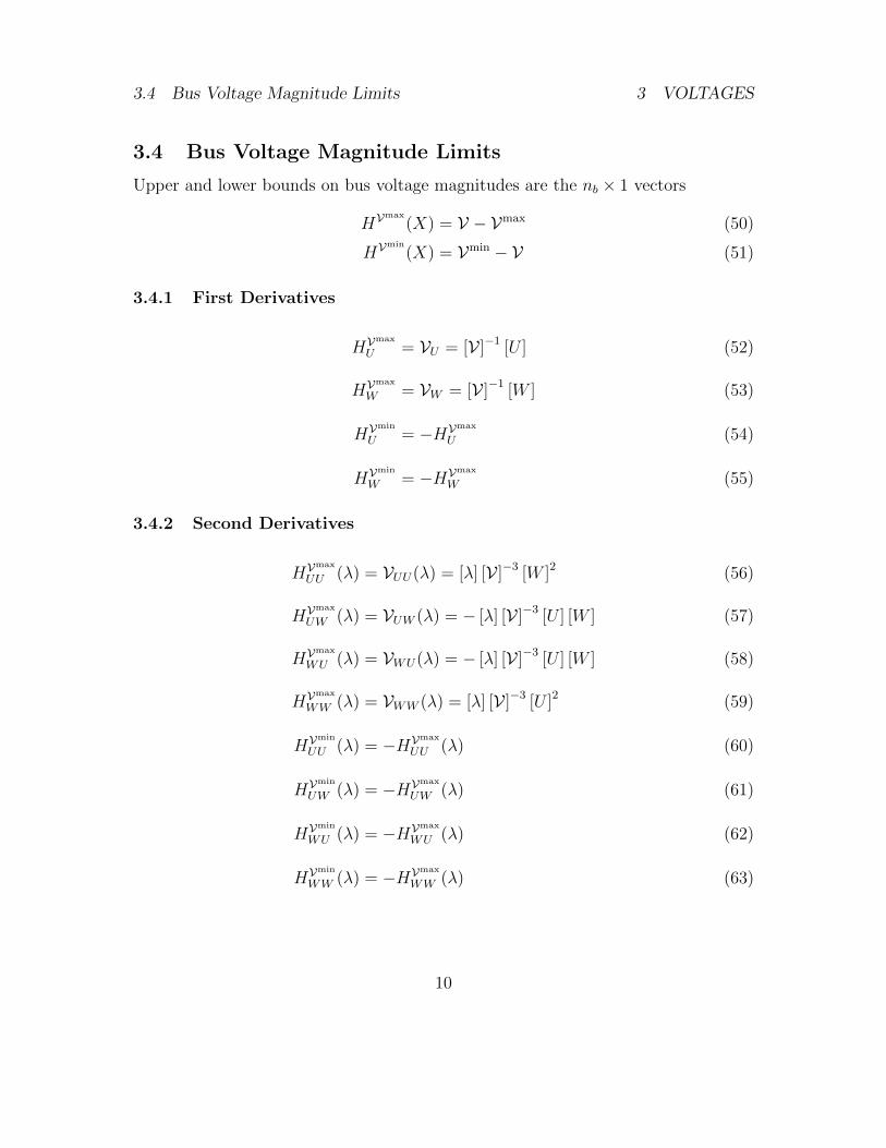
3.4 Bus Voltage Magnitude Limits

Upper and lower bounds on bus voltage magnitudes are the nb × 1 vectors

HVmax

(X) = V − Vmax (50)

HVmin

(X) = Vmin − V (51)


HVmax

U = VU = [V ]−1 [U ] (52)

HVmax

W = VW = [V ]−1 [W ] (53)

HVmin

U = −HVmax

U (54)

HVmin

W = −HVmax

W (55)


HVmax

UU (λ) = VUU(λ) = [λ] [V ]−3 [W ]2 (56)

HVmax

UW (λ) = VUW (λ) = − [λ] [V ]−3 [U ] [W ] (57)

HVmax

WU (λ) = VWU(λ) = − [λ] [V ]−3 [U ] [W ] (58)

HVmax

WW (λ) = VWW (λ) = [λ] [V ]−3 [U ]2 (59)

HVmin

UU (λ) = −HVmax

UU (λ) (60)

HVmin

UW (λ) = −HVmax

UW (λ) (61)

HVmin

WU (λ) = −HVmax

WU (λ) (62)

HVmin

WW (λ) = −HVmax

WW (λ) (63)

10

3.5 Branch Angle Difference Limits 3 VOLTAGES

3.5 Branch Angle Difference Limits

Upper and lower bounds on branch voltage angle differences are the nl × 1 vectors

HΘmax

(X) = (Cf − Ct)Θ−Θmaxft (64)

HΘmin

(X) = Θminft − (Cf − Ct)Θ (65)


HΘmax

U = (Cf − Ct)ΘU = −(Cf − Ct) [V ]−2 [W ] (66)

HΘmax

W = ΘW = (Cf − Ct) [V ]−2 [U ] (67)

HΘmin

U = −HΘmax

U (68)

HΘmin

W = −HΘmax

W (69)


HΘmax

UU (λ) = (Cf − Ct)ΘUU(λ) = 2(Cf − Ct) [λ] [V ]−4 [U ] [W ] (70)

HΘmax

UW (λ) = (Cf − Ct)ΘUW (λ) = (Cf − Ct) [λ] [V ]−4 ([W ]2 − [U ]2)

(71)

HΘmax

WU (λ) = (Cf − Ct)ΘWU(λ) = (Cf − Ct) [λ] [V ]−4 ([W ]2 − [U ]2)

(72)

HΘmax

WW (λ) = (Cf − Ct)ΘWW (λ) = −2(Cf − Ct) [λ] [V ]−4 [U ] [W ] (73)

HΘmin

UU (λ) = −HΘmax

UU (λ) (74)

HΘmin

UW (λ) = −HΘmax

UW (λ) (75)

HΘmin

WU (λ) = −HΘmax

WU (λ) (76)

HΘmin

WW (λ) = −HΘmax

WW (λ) (77)

11

4 BUS INJECTIONS

4 Bus Injections

4.1 Complex Current Injections

Consider the complex current balance equation, Gc(X) = 0, where

Gc(X) = Ibus + Idg (78)

and

Ibus = YbusV (79)

Idg = [Sd − CgSg]∗Λ∗ (80)


IbusX =

∂Ibus

∂X=[IbusU Ibus

W 0 0]

(81)

IbusU =

∂Ibus

∂U= Ybus

∂V

∂U= Ybus (82)

IbusW =

∂Ibus

∂W= Ybus

∂V

∂W= jYbus (83)

IdgX =∂Idg

∂X=[IdgU IdgW IdgPg

IdgQg

](84)

IdgU =∂Idg

∂U= −[Sd − CgSg]∗ [Λ∗]2 (85)

IdgW =∂Idg

∂W= j[Sd − CgSg]∗ [Λ∗]2 (86)

IdgPg=∂Idg

∂Pg= − [Λ∗]Cg (87)

IdgQg=∂Idg

∂Qg

= j [Λ∗]Cg (88)

12

4.1 Complex Current Injections 4 BUS INJECTIONS

GcX =

∂Gc

∂X=[GcU Gc

W GcPg

GcQg

](89)

GcU =

∂Gc

∂U= Ibus

U + IdgU = Ybus − [Sd − CgSg]∗ [Λ∗]2 (90)

GcW =

∂Gc

∂W= Ibus

W + IdgW = j(Ybus + [Sd − CgSg]∗ [Λ∗]2

)(91)

GcPg

=∂Gc

∂Pg= IdgPg

= − [Λ∗]Cg (92)

GcQg

=∂Gc

∂Qg

= IdgQg= j [Λ∗]Cg (93)


IbusXX(λ) =

∂

∂X

(IbusX

Tλ)

= 0 (94)

IdgXX(λ) =∂

∂X

(IdgX

Tλ)

(95)

=

IdgUU(λ) IdgUW (λ) IdgUPg

(λ) IdgUQg(λ)

IdgWU(λ) IdgWW (λ) IdgWPg(λ) IdgWQg

(λ)

IdgPgU(λ) IdgPgW

(λ) 0 0

IdgQgU(λ) IdgQgW

(λ) 0 0

(96)

=

C −jC DT −jDT

−jC −C −jDT −DT

D −jD 0 0−jD −D 0 0

(97)

IdgUU(λ) =∂

∂U

(IdgU

Tλ)

(98)

=∂

∂U

(−[Sd − CgSg]∗ [Λ∗]2 λ

)(99)

13


= −2[Sd − CgSg]∗ [λ] [Λ∗] Λ∗U (100)

= 2[Sd − CgSg]∗ [λ] [Λ∗]3 (101)

= C (102)

IdgWU(λ) =∂

∂U

(IdgW

Tλ)

(103)

=∂

∂U

(j[Sd − CgSg]∗ [Λ∗]2 λ

)(104)

= 2j[Sd − CgSg]∗ [λ] [Λ∗] Λ∗U (105)

= −2j[Sd − CgSg]∗ [λ] [Λ∗]3 (106)

= −jC (107)

IdgPgU(λ) =

∂

∂U

(IdgPg

Tλ)

(108)

=∂

∂U

(−CgT [Λ∗]λ

)(109)

= −CgT [λ] Λ∗U (110)

= CgT [λ] [Λ∗]2 (111)

= D (112)

IdgQgU(λ) =

∂

∂U

(IdgQg

Tλ)

(113)

=∂

∂U

(jCg

T [Λ∗]λ)

(114)

= jCgT [λ] Λ∗U (115)

= −jCgT [λ] [Λ∗]2 (116)

= −jD (117)

IdgUW (λ) =∂

∂W

(IdgU

Tλ)

(118)

=∂

∂W

(−[Sd − CgSg]∗ [Λ∗]2 λ

)(119)

= −2[Sd − CgSg]∗ [λ] [Λ∗] Λ∗W (120)

14


= −2j[Sd − CgSg]∗ [λ] [Λ∗]3 (121)

= IdgWU

T(λ) = −jC (122)

IdgWW (λ) =∂

∂W

(IdgW

Tλ)

(123)

=∂

∂W


)(124)

= 2j[Sd − CgSg]∗ [λ] [Λ∗] Λ∗W (125)

= −2[Sd − CgSg]∗ [λ] [Λ∗]3 (126)

= −C (127)

IdgPgW(λ) =

∂

∂W

(IdgPg

Tλ)

(128)

=∂

∂W

(−CgT [Λ∗]λ

)(129)

= −CgT [λ] Λ∗W (130)

= −jCgT [λ] [Λ∗]2 (131)

= −jD (132)

IdgQgW(λ) =

∂

∂W

(IdgQg

Tλ)

(133)

=∂

∂W

(jCg

T [Λ∗]λ)

(134)

= jCgT [λ] Λ∗W (135)

= −CgT [λ] [Λ∗]2 (136)

= −D (137)

IdgUPg(λ) =

∂

∂Pg

(IdgU

Tλ)

(138)

=∂

∂Pg

(−[Sd − CgSg]∗ [Λ∗]2 λ

)(139)

= [Λ∗]2 [λ]Cg (140)

15


= IdgPgU

T(λ) = DT (141)

IdgWPg(λ) =

∂

∂Pg

(IdgW

Tλ)

(142)

=∂

∂Pg


)(143)

= −j [Λ∗]2 [λ]Cg (144)

= IdgPgW

T(λ) = −jDT (145)

IdgUQg(λ) =

∂

∂Qg

(IdgU

Tλ)

(146)

=∂

∂Qg

(−[Sd − CgSg]∗ [Λ∗]2 λ

)(147)

= −j [Λ∗]2 [λ]Cg (148)

= IdgQgU

T(λ) = −jDT (149)

IdgWQg(λ) =

∂

∂Qg

(IdgW

Tλ)

(150)

=∂

∂Qg


)(151)

= − [Λ∗]2 [λ]Cg (152)

= IdgQgW

T(λ) = −DT (153)

GcXX(λ) =

∂

∂X

(GcX

Tλ)

(154)

=

GcUU(λ) Gc

UW (λ) GcUPg

(λ) GcUQg

(λ)

GcWU(λ) Gc

WW (λ) GcWPg

(λ) GcWQg

(λ)

GcPgU

(λ) GcPgW

(λ) 0 0

GcQgU

(λ) GcQgW

(λ) 0 0

(155)

= IdgXX(λ) (156)

16

4.2 Complex Power Injections 4 BUS INJECTIONS

=

C −jC DT −jDT

−jC −C −jDT −DT

D −jD 0 0−jD −D 0 0

(157)

Computational savings can be achieved by storing and reusing certain interme-diate terms during the computation of these second derivatives, as follows:

A = [Λ∗] (158)

B = [λ]A2 (159)

C = 2[Sd − CgSg]∗AB (160)

D = CgTB (161)

GcUU(λ) = C (162)

GcWU(λ) = −jC (163)

GcPgU(λ) = D (164)

GcQgU(λ) = −jD (165)

GcWW (λ) = −C (166)

GcPgW (λ) = −jD (167)

GcQgW (λ) = −D (168)

GcUW (λ) = Gc

WU(λ) (169)

GcUPg

(λ) = GcPgU

T(λ) (170)

GcWPg

(λ) = GcPgW

T(λ) (171)

GcUQg

(λ) = GcQgU

T(λ) (172)

GcWQg

(λ) = GcQgW

T(λ) (173)

4.2 Complex Power Injections

Consider the complex power balance equation, Gs(X) = 0, where

Gs(X) = Sbus + Sd − CgSg (174)

and

Sbus = [V ] Ibus∗ (175)

17



GsX =

∂Gs

∂X=[GsU Gs

W GsPg

GsQg

](176)

GsU =

∂Sbus

∂U=[Ibus∗

] ∂V∂U

+ [V ]∂Ibus∗

∂U(177)

=[Ibus∗

]+ [V ]Ybus

∗ (178)

GsW =

∂Sbus

∂W=[Ibus∗

] ∂V∂W

+ [V ]∂Ibus∗

∂W(179)

= j([Ibus∗

]− [V ]Ybus

∗)

(180)

GsPg

= −Cg (181)

GsQg

= −jCg (182)


GsXX(λ) =

∂

∂X

(GsX

Tλ)

(183)

=

GsUU(λ) Gs

UW (λ) 0 0GsWU(λ) Gs

WW (λ) 0 00 0 0 00 0 0 0

(184)

GsUU(λ) =

∂

∂U

(GsUTλ)

(185)

=∂

∂U

(([Ibus∗

]+ Ybus

∗T [V ])λ)

(186)

=∂

∂U

([λ]Ybus

∗V ∗ + Ybus∗T [λ]V

)(187)

= [λ]Ybus∗ + Ybus

∗T [λ] (188)

= F (189)

GsWU(λ) =

∂

∂U

(GsW

Tλ)

(190)

18


=∂

∂U

(j([Ibus∗

]− Ybus

∗T [V ])λ)

(191)

=∂

∂U

(j(

[λ]Ybus∗V ∗ − Ybus

∗T [λ]V))

(192)

= j(

[λ]Ybus∗ − Ybus

∗T [λ])

(193)

= G (194)

GsUW (λ) =

∂

∂W

(GsUTλ)

(195)

=∂

∂W

(([Ibus∗

]+ Ybus

∗T [V ])λ)

(196)

=∂

∂W

([λ]Ybus

∗V ∗ + Ybus∗T [λ]V

)(197)

= j(Ybus

∗T [λ]− [λ]Ybus∗)

(198)

= GsWU

T(λ) = GT (199)

GsWW (λ) =

∂

∂W

(GsW

Tλ)

(200)

=∂

∂W

(j([Ibus∗

]− Ybus

∗T [V ])λ)

(201)

=∂

∂W

(j(

[λ]Ybus∗V ∗ − Ybus

∗T [λ]V))

(202)

= [λ]Ybus∗ + Ybus

∗T [λ] (203)

= F (204)


E = [λ]Ybus∗ (205)

F = E + ET (206)

G = j(E − ET

)(207)

GsUU(λ) = F (208)

GsWU(λ) = G (209)

GsUW (λ) = GT (210)

GsWW (λ) = F (211)

19

5 BRANCH FLOWS

5 Branch Flows

Consider the line flow constraints of the form H(X) < 0. This section examines 3variations based on the square of the magnitude of the current, apparent power andreal power, respectively. The relationships are derived first for the complex flows atthe from ends of the branches. Derivations for the to end are identical (i.e. justreplace all f sub/super-scripts with t).

5.1 Complex Currents

If = YfV (212)

I t = YtV (213)


IfX =∂If

∂X=[IfU IfW IfPg

IfQg

](214)

IfU =∂If

∂U= Yf (215)

IfW =∂If

∂W= jYf (216)

IfPg=∂If

∂Pg= 0 (217)

IfQg=∂If

∂Qg

= 0 (218)


IfXX(µ) =∂

∂X

(IfX

Tµ)

= 0 (219)

5.2 Complex Power Flows

Sf = [Vf ] If ∗ (220)

St = [Vt] It∗ (221)

20

5.2 Complex Power Flows 5 BRANCH FLOWS


SfX =∂Sf

∂X=[SfU SfW SfPg

SfQg

](222)

=[If∗] ∂Vf∂X

+ [Vf ]∂If

∗

∂X(223)

SfU =[If∗] ∂Vf∂U

+ [Vf ]∂If

∗

∂U(224)

=[If∗]Cf + [Vf ]Yf

∗ (225)

SfW =[If∗] ∂Vf∂W

+ [Vf ]∂If

∗

∂W(226)

= j([If∗]Cf − [Vf ]Yf

∗)

(227)

SfPg= 0 (228)

SfQg= 0 (229)


SfXX(µ) =∂

∂X

(SfX

Tµ)

(230)

=

SfUU(µ) SfUW (µ) 0 0

SfWU(µ) SfWW (µ) 0 00 0 0 00 0 0 0

(231)

SfUU(µ) =∂

∂U

(SfU

Tµ)

(232)

=∂

∂U

((Cf

T[If∗]

+ Yf∗T [Vf ]

)µ)

(233)

= CfT [µ]

∂If∗

∂U+ Yf

∗T [µ]∂Vf∂U

(234)

= CfT [µ]Yf

∗ + Yf∗T [µ]Cf (235)

21

5.2 Complex Power Flows 5 BRANCH FLOWS

= Bf (236)

SfWU(µ) =∂

∂U

(SfW

Tµ)

(237)

=∂

∂U

(j(Cf

T[If∗]− Yf ∗T [Vf ]

)µ)

(238)

= j

(Cf

T [µ]∂If

∗

∂U− Yf ∗T [µ]

∂Vf∂U

)(239)

= j(Cf

T [µ]Yf∗ − Yf ∗T [µ]Cf

)(240)

= Df (241)

SfUW (µ) =∂

∂W

(SfU

Tµ)

(242)

=∂

∂W

((Cf

T[If∗]

+ Yf∗T [Vf ]

)µ)

(243)

= CfT [µ]

∂If∗

∂W+ Yf

∗T [µ]∂Vf∂W

(244)

= −j(Cf

T [µ]Yf∗ − Yf ∗T [µ]Cf

)(245)

= SfWU

T(µ) = −Df (246)

SfWW (µ) =∂

∂W

(SfW

Tµ)

(247)

=∂

∂W

(j(Cf

T[If∗]− Yf ∗T [Vf ]

)µ)

(248)

= j

(Cf

T [µ]∂If

∗

∂W− Yf ∗T [µ]

∂Vf∂W

)(249)

= j(Cf

T [µ] (−j)Yf ∗ − Yf ∗T [µ] (j)Cf

)(250)

= CfT [µ]Yf

∗ + Yf∗T [µ]Cf (251)

= Bf (252)


Af = CfT [µ]Yf

∗ (253)

22

5.3 Squared Current Magnitudes 6 GENERALIZED AC OPF COSTS

Bf = Af +AfT (254)

Df = j(Af −AfT

)(255)

SfUU(µ) = Bf (256)

SfWU(µ) = Df (257)

SfUW (µ) = SfWU

T(µ) = −Df (258)

SfWW (µ) = Bf (259)

5.3 Squared Current Magnitudes

See the corresponding section in Matpower Technical Note 2.

5.4 Squared Apparent Power Magnitudes


5.5 Squared Real Power Magnitudes


6 Generalized AC OPF Costs

Let X be defined as

X =

UWPgQg

YZ

(260)

where Y is the ny×1 vector of cost variables associated with piecewise linear generatorcosts and Z is an nz × 1 vector of additional linearly constrained user variables.

See the corresponding section in Matpower Technical Note 2 for additionaldetails.

23





7 LAGRANGIAN OF THE AC OPF

7 Lagrangian of the AC OPF

Consider the following AC OPF problem formulation, where X is defined as in (260),f is the cost function, and X represents the reduced form of X, consisting of onlyU , W , Pg and Qg, without Y and Z.

minX

f(X) (261)

subject to

G(X) = 0 (262)

H(X) ≤ 0 (263)

where

G(X) =

<{Gb(X )}={Gb(X )}Gref(X )

AEX −BE

(264)

and

H(X) =

Hf (X )H t(X )

HVmax

(X )

HVmin

(X )HΘmax

(X )

HΘmin(X )

AIX −BI

(265)

and Gb is the nodal balance function, equal to either Gc for current balance or to Gs

for power balance.Partitioning the corresponding multipliers λ and µ similarly,

λ =

λPλQλref

λE

, µ =

µfµt

µVmax

µVmin

µΘmax

µΘmin

µI

(266)

the Lagrangian for this problem can be written as

L(X,λ, µ) = f(X) + λTG(X) + µTH(X) (267)

24

7.1 Nodal Current Balance 7 LAGRANGIAN OF THE AC OPF

7.1 Nodal Current Balance

Let the nodal balance function Gb be the nodal complex current balance Gc.


LX(X,λ, µ) = fX + λTGX + µTHX (268)

Lλ(X,λ, µ) = GT(X) (269)

Lµ(X,λ, µ) = HT(X) (270)

where

GX =

<{Gc

X} 0 0={Gc

X} 0 0GrefX 0 0

AE

=

<{Gc

U} <{GcW} <{Gc

Pg} <{Gc

Qg} 0 0

={GcU} ={Gc

W} ={GcPg} ={Gc

Qg} 0 0

GrefU Gref

W 0 0 0 0AE

(271)

and

HX =

HfX 0 0

H tX 0 0

HVmax

X 0 0

HVmin

X 0 0HΘmax

X 0 0

HΘmin

X 0 0AI

=

HfU Hf

W 0 0 0 0H tU H t

W 0 0 0 0HV

max

U HVmax

W 0 0 0 0

HVmin

U HVmin

W 0 0 0 0HΘmax

U HΘmax

W 0 0 0 0

HΘmin

U HΘmin

W 0 0 0 0AI

(272)


LXX(X,λ, µ) = fXX +GXX(λ) +HXX(µ) (273)

where

GXX(λ) =

GXX (λ) 0 00 0 00 0 0

(274)

25

7.1 Nodal Current Balance 7 LAGRANGIAN OF THE AC OPF

GXX (λ) = <{GcXX (λP )}+ ={Gc

XX (λQ)}+GrefXX (λref) (275)

= <

GcUU(λP ) Gc

UW (λP ) GcUPg

(λP ) GcUQg

(λP )

GcWU(λP ) Gc

WW (λP ) GcWPg

(λP ) GcWQg

(λP )

GcPgU

(λP ) GcPgW

(λP ) 0 0

GcQgU

(λP ) GcQgW

(λP ) 0 0

+ =

GcUU(λQ) Gc

UW (λQ) GcUPg

(λQ) GcUQg

(λQ)

GcWU(λQ) Gc

WW (λQ) GcWPg

(λQ) GcWQg

(λQ)

GcPgU

(λQ) GcPgW

(λQ) 0 0

GcQgU

(λQ) GcQgW

(λQ) 0 0

+

GrefUU(λref) Gref

UW (λref) 0 0GrefWU(λref) Gref

WW (λref) 0 00 0 0 00 0 0 0

(276)

and

HXX(µ) =

HXX (µ) 0 00 0 00 0 0

(277)

HXX (µ) =

HUU(µ) HUW (µ) 0 0HWU(µ) HWW (µ) 0 0

0 0 0 00 0 0 0

(278)

HUU(µ) = HfUU(µf ) +H t

UU(µt)

+HVmax

UU (µVmax) +HVmin

UU (µVmin)

+HΘmax

UU (µΘmax) +HΘmin

UU (µΘmin) (279)

HUW (µ) = HfUW (µf ) +H t

UW (µt)

+HVmax

UW (µVmax) +HVmin

UW (µVmin)

+HΘmax

UW (µΘmax) +HΘmin

UW (µΘmin) (280)

HWU(µ) = HfWU(µf ) +H t

WU(µt)

+HVmax

WU (µVmax) +HVmin

WU (µVmin)

26

7.2 Nodal Power Balance 7 LAGRANGIAN OF THE AC OPF

+HΘmax

WU (µΘmax) +HΘmin

WU (µΘmin) (281)

HWW (µ) = HfWW (µf ) +H t

WW (µt)

+HVmax

WW (µVmax) +HVmin

WW (µVmin)

+HΘmax

WW (µΘmax) +HΘmin

WW (µΘmin) (282)

7.2 Nodal Power Balance

Let the nodal balance function Gb be the nodal complex power balance Gs.


LX(X,λ, µ) = fX + λTGX + µTHX (283)

Lλ(X,λ, µ) = GT(X) (284)

Lµ(X,λ, µ) = HT(X) (285)

where

GX =

<{Gs

X} 0 0={Gs

X} 0 0GrefX 0 0

AE

=

<{Gs

U} <{GsW} −Cg 0 0 0

={GsU} ={Gs

W} 0 −Cg 0 0GrefU Gref

W 0 0 0 0AE

(286)

and HX is the same as for nodal current balance in (272).


LXX(X,λ, µ) = fXX +GXX(λ) +HXX(µ) (287)

where

GXX(λ) =

GXX (λ) 0 00 0 00 0 0

(288)

27

7.2 Nodal Power Balance 7 LAGRANGIAN OF THE AC OPF

GXX (λ) = <{GsXX (λP )}+ ={Gs

XX (λQ)}+GrefXX (λref) (289)

= <

GsUU(λP ) Gs

UW (λP ) 0 0GsWU(λP ) Gs

WW (λP ) 0 00 0 0 00 0 0 0

+ =

GsUU(λQ) Gs

UW (λQ) 0 0GsWU(λQ) Gs

WW (λQ) 0 00 0 0 00 0 0 0

+

GrefUU(λref) Gref

UW (λref) 0 0GrefWU(λref) Gref

WW (λref) 0 00 0 0 00 0 0 0

(290)

and HXX(µ) is the same as for nodal current balance in (277)–(282).

28

8 REVISION HISTORY

8 Revision History

• Revision 2 (Jume 20, 2019) – Added separate references for Matpowersoftware and User’s Manual. Included DOIs for all Matpower software, User’sManual and Technical Note references. Updated Matpower website links tohttps://matpower.org.

• Revision 1 (October 25, 2018)

– Added missing equality constraint for reference voltage angles. See Sec-tions 3.3 and 7.

– Added missing inequality constraints for bus voltage magnitude limits.See Sections 3.4 and 7.

– Added missing inequality constraints for branch voltage angle differencelimits. See Sections 3.5 and 7.

• Initial version (April 2, 2018) – Published as “Matpower Technical Note 4”.

29

https://matpower.org

https://matpower.org/docs/TN4-OPF-Derivatives-Cartesian.pdf

A SCALAR POLAR COORDINATE DERIVATIVES

Appendix A Scalar Polar Coordinate Derivatives

When using cartesian coordinates for the voltages, the voltage magnitudes and anglesare now functions of the cartesian coordinates. Constraints on these functions requiretheir derivatives as well.

Consider a scalar complex voltage v that can be expressed in polar coordinates|v| and θ or cartesian coordinates u and w as:

v = |v|ejθ (291)

= u+ jw (292)

We also have

θ = tan−1 w

u(293)

|v|2 = u2 + w2 (294)

A.1 First Derivatives

Given that∂ tan−1(y)

∂x=

1

1 + y2

∂y

∂x(295)

we have

∂θ

∂u=

1

1 + u−2w2

∂(u−1w)

∂u=

1

1 + u−2w2(−u−2w) = − w

|v|2(296)

∂θ

∂w=

1

1 + u−2w2

∂(u−1w)

∂w=

1

1 + u−2w2u−1 =

u

|v|2(297)

∂|v|∂u

=∂|v|∂|v|2

∂|v|2

∂u=

1

2(|v|2)−

12 (2u) =

u

|v|(298)

∂|v|∂w

=∂|v|∂|v|2

∂|v|2

∂w=

1

2(|v|2)−

12 (2w) =

w

|v|(299)

30

A.2 Second Derivatives A SCALAR POLAR COORDINATE DERIVATIVES

A.2 Second Derivatives

∂2θ

∂u2=∂(−|v|−2w)

∂u= −w(−2|v|−3)

u

|v|=

2uw

|v|4(300)

∂2θ

∂w∂u=∂(|v|−2u)

∂u=

1

|v|2+ u

(−2

|v|3

)u

|v|=|v|2 − 2u2

|v|4=w2 − u2

|v|4(301)

∂2θ

∂u∂w=∂(−|v|−2w)

∂w= − 1

|v|2− w

(−2

|v|3

)w

|v|=−|v|2 + 2w2

|v|4(302)

=w2 − u2

|v|4=

∂2θ

∂w∂u(303)

∂2θ

∂w2=∂(|v|−2u)

∂w= u(−2|v|−3)

w

|v|= −2uw

|v|4= −∂

2θ

∂u2(304)

∂2|v|∂u2

=∂(|v|−1u)

∂u= |v|−1 + u(−|v|−2)

u

|v|=|v|2 − u2

|v|3=

w2

|v|3(305)

∂2|v|∂w∂u

=∂(|v|−1w)

∂u= w(−|v|−2)

u

|v|= − uw|v|3

(306)

∂2|v|∂u∂w

=∂(|v|−1u)

∂w= u(−|v|−2)

w

|v|= − uw|v|3

=∂2|v|∂w∂u

(307)

∂2|v|∂w2

=∂(|v|−1w)

∂w= |v|−1 + w(−|v|−2)

w

|v|=|v|2 − w2

|v|3=

u2

|v|3(308)

31

REFERENCES REFERENCES

References

[1] R. D. Zimmerman, AC Power Flows, Generalized OPF Costs andtheir Derivatives using Complex Matrix Notation, Matpower TechnicalNote 2, February 2010. [Online]. Available: https://matpower.org/docs/

TN2-OPF-Derivatives.pdf

doi: 10.5281/zenodo.3237866 2

[2] B. Sereeter and R. D. Zimmerman, Addendum to AC Power Flows and theirDerivatives using Complex Matrix Notation: Nodal Current Balance, Mat-power Technical Note 3, April 2018. [Online]. Available: https://matpower.

org/docs/TN3-More-OPF-Derivatives.pdf

doi: 10.5281/zenodo.3237900 2

[3] R. D. Zimmerman, C. E. Murillo-Sanchez, and R. J. Thomas, “Matpower:Steady-State Operations, Planning and Analysis Tools for Power Systems Re-search and Education,” Power Systems, IEEE Transactions on, vol. 26, no. 1,pp. 12–19, Feb. 2011.doi: 10.1109/TPWRS.2010.2051168 2

[4] R. D. Zimmerman, C. E. Murillo-Sanchez (2019). Matpower[Software]. Available: https://matpower.orgdoi: 10.5281/zenodo.3236535 2

[5] R. D. Zimmerman, C. E. Murillo-Sanchez. Matpower User’s Manual. 2019.[Online]. Available: https://matpower.org/docs/MATPOWER-manual.pdfdoi: 10.5281/zenodo.3236519 2

32





https://doi.org/10.5281/zenodo.3237866






https://doi.org/10.1109/TPWRS.2010.2051168

https://matpower.org


https://matpower.org/docs/MATPOWER-manual.pdf


Documents

AC Power Flows and their Derivatives using …AC Power Flows and their Derivatives using Complex Matrix Notation and Cartesian Coordinate Voltages Baljinnyam Sereeter Ray D. Zimmerman