Abstracts - University of Warwick

The R User Conference, useR! 2011August 16-18 2011

University of Warwick, Coventry, UK

Book of Contributed Abstracts

Compiled 2011-07-28

1

Contents

Tuesday 16th August 5

Kaleidoscope Ia, 09:50-10:50 5Spectroscopic Data in R and Validation of Soft Classifiers: Classifying Cells and Tissues by Raman

Spectroscopy . . . . . . . . . . . . . . . . . . . . . . . . . . . . . . . . . . . . . . . . . . . . . . . . 6Revisiting Multi-Subject Random Effects in fMRI . . . . . . . . . . . . . . . . . . . . . . . . . . . . . . 7Putting the R into Randomisation . . . . . . . . . . . . . . . . . . . . . . . . . . . . . . . . . . . . . . . 8

Kaleidoscope Ib, 09:50-10:50 9Bringing the power of complex data analysis methods into R . . . . . . . . . . . . . . . . . . . . . . . . 9Using the Google Visualisation API with R . . . . . . . . . . . . . . . . . . . . . . . . . . . . . . . . . . 10Experimenting with a TTY connection for R . . . . . . . . . . . . . . . . . . . . . . . . . . . . . . . . . 11

Kaleidoscope Ic, 09:50-10:50 12The R Ecosystem . . . . . . . . . . . . . . . . . . . . . . . . . . . . . . . . . . . . . . . . . . . . . . . . . 12Rc2: R collaboration in the cloud . . . . . . . . . . . . . . . . . . . . . . . . . . . . . . . . . . . . . . . . 13RStudio: Integrated Development Environment for R . . . . . . . . . . . . . . . . . . . . . . . . . . . . 14

Portfolio Management, 11:15-12:35 15R in the Practice of Risk Management Today . . . . . . . . . . . . . . . . . . . . . . . . . . . . . . . . . 15Stress Testing with R-Adamant . . . . . . . . . . . . . . . . . . . . . . . . . . . . . . . . . . . . . . . . . 16Handling Multiple Time Scales in Hedge Fund Index Products . . . . . . . . . . . . . . . . . . . . . . . 17

Bioinformatics and High-throughput Data, 11:15-12:35 18AFLP: generating objective and repeatable genetic data . . . . . . . . . . . . . . . . . . . . . . . . . . . 18The nz.seq package for handling genetic sequences in the Netezza Performance Server . . . . . . . . . . 19Classification of Coverage Patterns . . . . . . . . . . . . . . . . . . . . . . . . . . . . . . . . . . . . . . . 20Finite Mixture Model Clustering of SNP Data . . . . . . . . . . . . . . . . . . . . . . . . . . . . . . . . . 21

High Performance Computing, 11:15-12:35 22GPU computing and R . . . . . . . . . . . . . . . . . . . . . . . . . . . . . . . . . . . . . . . . . . . . . 22Deploying and Benchmarking R on a Large Shared Memory System . . . . . . . . . . . . . . . . . . . . 23The CUtil package which enables GPU computation in R . . . . . . . . . . . . . . . . . . . . . . . . . . 24OBANSoft: integrated software for Bayesian statistics and high performance computing with R . . . . . 25

Reporting Technologies and Workflows, 11:15-12:35 26R2wd: writing Word Documents from R . . . . . . . . . . . . . . . . . . . . . . . . . . . . . . . . . . . . 26FRAD - Fast Results Analysis and Display . . . . . . . . . . . . . . . . . . . . . . . . . . . . . . . . . . 27The Emacs Org-mode: Reproducible Research and Beyond . . . . . . . . . . . . . . . . . . . . . . . . . 28Efficient data analysis workflow in R . . . . . . . . . . . . . . . . . . . . . . . . . . . . . . . . . . . . . . 29

Teaching, 11:15-12:35 30Teaching Statistics to Psychology Students using Reproducible Computing package RC and supporting

Peer Review Framework . . . . . . . . . . . . . . . . . . . . . . . . . . . . . . . . . . . . . . . . . . 30Teaching applied statistics to students in natural sciences using the R Commander . . . . . . . . . . . . 31Automatic generation of exams in R . . . . . . . . . . . . . . . . . . . . . . . . . . . . . . . . . . . . . . 32

Modelling Systems and Networks, 16:00-17:00 33An S4 Object structure for emulation - the approximation of complex functions . . . . . . . . . . . . . . 33The structmcmc package: Structural inference of Bayesian networks using MCMC . . . . . . . . . . . . 34Computation of generalized Nash equilibria . . . . . . . . . . . . . . . . . . . . . . . . . . . . . . . . . . 35

Computational Physics and Chemometrics, 16:00-17:00 36Segmented regression in thermo-physics modeling . . . . . . . . . . . . . . . . . . . . . . . . . . . . . . . 36Sparse Bayesian kernel projections for classification of near-infrared spectroscopy data . . . . . . . . . . 37Recovering Signals and Information From Radio Frequencies Using R (A high school student’s experience) 38

Visualisation, 16:00-17:00 39animatoR: dynamic graphics in R . . . . . . . . . . . . . . . . . . . . . . . . . . . . . . . . . . . . . . . . 39Graphical Syntax for Structables and their Mosaic Plots . . . . . . . . . . . . . . . . . . . . . . . . . . . 40RMB: Visualising categorical data with Relative Multiple Barcharts . . . . . . . . . . . . . . . . . . . . 41

2

Official and Social Statistics, 16:00-17:00 42ObsSensitivity: An R package for power analysis for sensitivity analyses of Observational Studies . . . . 42Visualizing Multilevel Propensity Score Analysis . . . . . . . . . . . . . . . . . . . . . . . . . . . . . . . 43

Dimensionality Reduction and Variable Selection, 16:00-17:00 44ClustOfVar: an R package for the clustering of variables . . . . . . . . . . . . . . . . . . . . . . . . . . . 44Variable Screening and Parameter Estimation for High-Dimensional Generalized Linear Mixed Models

Using L1-Penalization . . . . . . . . . . . . . . . . . . . . . . . . . . . . . . . . . . . . . . . . . . . 45gamboostLSS: boosting generalized additive models for location, scale and shape . . . . . . . . . . . . . 46

Business Management, 16:00-17:00 47SCperf: An inventory management package for R . . . . . . . . . . . . . . . . . . . . . . . . . . . . . . . 47Using R to test transaction cost measurement for supply chain relationship: A structural equation model 48Integrating R and Excel for automatic business forecasting . . . . . . . . . . . . . . . . . . . . . . . . . 49

Wednesday 17th August 50

Kaleidoscope IIa, 09:50-10:50 50Using R to quantify the buildup in extent of free exploration in mice . . . . . . . . . . . . . . . . . . . . 50Changepoint analysis with the changepoint package in R . . . . . . . . . . . . . . . . . . . . . . . . . . . 51Clustering patterns in streamflow to produce regionally or anthropogenically similar groups . . . . . . . 52

Panel Discussion I, 09:50-10:50 53R User Group Panel . . . . . . . . . . . . . . . . . . . . . . . . . . . . . . . . . . . . . . . . . . . . . . . 53

Kaleidoscope IIb, 09:50-10:50 54RTextTools . . . . . . . . . . . . . . . . . . . . . . . . . . . . . . . . . . . . . . . . . . . . . . . . . . . . 54The Role of R in Lab Automation . . . . . . . . . . . . . . . . . . . . . . . . . . . . . . . . . . . . . . . 55Using R data functions with TIBCO Spotfire . . . . . . . . . . . . . . . . . . . . . . . . . . . . . . . . . 56

Spatio-Temporal Statistics, 11:15-12:35 57Spatio-Temporal Bayesian Modelling using R . . . . . . . . . . . . . . . . . . . . . . . . . . . . . . . . . 57Applying geospatial techniques to temporal data . . . . . . . . . . . . . . . . . . . . . . . . . . . . . . . 58Structured Additive Regression Models: An R Interface to BayesX . . . . . . . . . . . . . . . . . . . . . 59

Molecular and Cell Biology, 11:15-12:35 60The R package isocir for Isotonic Inference for Circular Data. Applications to Problems Encountered in

Cell Biology. . . . . . . . . . . . . . . . . . . . . . . . . . . . . . . . . . . . . . . . . . . . . . . . . 60CircNNTSR: An R Package for the Statistical Analysis of Circular Data Based on Nonnegative Trigono-

metric Sums . . . . . . . . . . . . . . . . . . . . . . . . . . . . . . . . . . . . . . . . . . . . . . . . . 61Summary statistics selection for ABC inference in R . . . . . . . . . . . . . . . . . . . . . . . . . . . . . 62Power and minimal sample size for multivariate analysis of microarrays . . . . . . . . . . . . . . . . . . 63

Mixed Effect Models, 11:15-12:35 64Kenward-Roger modification of the F-statistic for some linear mixed models fitted with lmer . . . . . . 64lqmm: Estimating Quantile Regression Models for Independent and Hierarchical Data with R . . . . . . 65lcmm: an R package for estimation of latent class mixed models and joint latent class models . . . . . . 66Mixed-effects Maximum Likelihood Difference Scaling . . . . . . . . . . . . . . . . . . . . . . . . . . . . 67

Programming, 11:15-12:35 68Tricks and Traps for Young Players . . . . . . . . . . . . . . . . . . . . . . . . . . . . . . . . . . . . . . . 68Software design patterns in R . . . . . . . . . . . . . . . . . . . . . . . . . . . . . . . . . . . . . . . . . . 69Random input testing with R . . . . . . . . . . . . . . . . . . . . . . . . . . . . . . . . . . . . . . . . . . 70An Open Source Visual R Debugger in StatET . . . . . . . . . . . . . . . . . . . . . . . . . . . . . . . . 71

Data Mining Applications, 11:15-12:35 72Predicting the offender’s age . . . . . . . . . . . . . . . . . . . . . . . . . . . . . . . . . . . . . . . . . . . 72Leveraging Online Social Network Data and External Data Sources to Predict Personality . . . . . . . . 73Using R to Model Click-Stream Data to Understand Users’ Path To Conversion . . . . . . . . . . . . . . 74

3

Development of R, 16:00-17:00 75Packaging R for Ubuntu: Recent Changes and Future Opportunities . . . . . . . . . . . . . . . . . . . . 75Interpreter Internals: Unearthing Buried Treasure with CXXR . . . . . . . . . . . . . . . . . . . . . . . 76R’s Participation in the Google Summer of Code 2011 . . . . . . . . . . . . . . . . . . . . . . . . . . . . 77

Geospatial Techniques, 16:00-17:00 78Converting a spatial network to a graph in R . . . . . . . . . . . . . . . . . . . . . . . . . . . . . . . . . 78Spatial modelling with the R–GRASS Interface . . . . . . . . . . . . . . . . . . . . . . . . . . . . . . . . 79sos4R - Accessing SensorWeb Data from R . . . . . . . . . . . . . . . . . . . . . . . . . . . . . . . . . . 80

Genomics and Bioinformatics, 16:00-17:00 81MALDIquant: Quantitative Analysis of MALDI-TOF Proteomics Data . . . . . . . . . . . . . . . . . . 81QuACN: Analysis of Complex Biological Networks using R . . . . . . . . . . . . . . . . . . . . . . . . . 82Investigate clusters of co-expressed and co-located genes at a genomic scale using CoCoMap . . . . . . . 83

Regression Modelling, 16:00-17:00 84Beta Regression: Shaken, Stirred, Mixed, and Partitioned . . . . . . . . . . . . . . . . . . . . . . . . . . 84Regression Models for Ordinal Data: Introducing R-package ordinal . . . . . . . . . . . . . . . . . . . . 85Multiple choice models: why not the same answer? A comparison among LIMDEP, R, SAS and Stata. . 86

R in the Business World, 16:00-17:00 87Odesseus vs. Ajax: How to build an R presence in a corporate SAS environment . . . . . . . . . . . . . 87A Validation/Qualification Solution for R . . . . . . . . . . . . . . . . . . . . . . . . . . . . . . . . . . . 88R as a statistical tool for human factor engineering . . . . . . . . . . . . . . . . . . . . . . . . . . . . . . 89

Hydrology and Soil Science, 17:05-18:05 90GWSDAT (GroundWater Spatiotemporal Data Analysis Tool) . . . . . . . . . . . . . . . . . . . . . . . 90IntR – Interactive GUI for R . . . . . . . . . . . . . . . . . . . . . . . . . . . . . . . . . . . . . . . . . . 91Visualisation and modelling of soil data using the aqp package . . . . . . . . . . . . . . . . . . . . . . . 92

Biostatistical Modelling, 17:05-18:05 93survAUC: Estimators of Prediction Accuracy for Time-to-Event Data . . . . . . . . . . . . . . . . . . . 93Higher-order likelihood inference in meta-analysis using R . . . . . . . . . . . . . . . . . . . . . . . . . . 94Gaussian copula regression using R . . . . . . . . . . . . . . . . . . . . . . . . . . . . . . . . . . . . . . . 95

Psychometrics, 17:05-18:05 96Multinomial Processing Tree Models in R . . . . . . . . . . . . . . . . . . . . . . . . . . . . . . . . . . . 96Detecting Invariance in Psychometric Models with the psychotree Package . . . . . . . . . . . . . . . . . 97Investigating multidimensional unfolding models using R2WinBUGS . . . . . . . . . . . . . . . . . . . . 98

Multivariate Data, 17:05-18:05 99Tests for Multivariate Linear Models with the car Package . . . . . . . . . . . . . . . . . . . . . . . . . . 99missMDA: a package to handle missing values in and with multivariate exploratory data analysis methods100MAINT.DATA: Modeling and Analysing Interval Data in R . . . . . . . . . . . . . . . . . . . . . . . . . 101

Interfaces, 17:05-18:05 102Web 2.0 for R scripts & workflows: Tiki & PluginR . . . . . . . . . . . . . . . . . . . . . . . . . . . . . . 102Browser Based Applications Supported by R in Pipeline Pilot . . . . . . . . . . . . . . . . . . . . . . . . 103A new task-based GUI for R . . . . . . . . . . . . . . . . . . . . . . . . . . . . . . . . . . . . . . . . . . 104

Thursday 18th August 105

Financial Models, 09:50-10:50 105Computational aspects of continuous-time-arma (CARMA) models: The ctarma package . . . . . . . . . 105robKalman - An R package for robust Kalman filtering revisited . . . . . . . . . . . . . . . . . . . . . . 106(Robust) Online Filtering in Regime Switching Models and Application to Investment Strategies for

Asset Allocation . . . . . . . . . . . . . . . . . . . . . . . . . . . . . . . . . . . . . . . . . . . . . . 107

Ecology and Ecological Modelling, 09:50-10:50 108Using R for the Analysis of Bird Demography on a Europe-wide Scale . . . . . . . . . . . . . . . . . . . 108Using OpenBUGS and lmer to study variation in plant demographic rates over several spatial and

temporal scales . . . . . . . . . . . . . . . . . . . . . . . . . . . . . . . . . . . . . . . . . . . . . . . 109An effort to improve nonlinear modeling practice . . . . . . . . . . . . . . . . . . . . . . . . . . . . . . . 110

4

Generalized Linear Models, 09:50-10:50 111brglm: Bias reduction in generalized linear models . . . . . . . . . . . . . . . . . . . . . . . . . . . . . . 111Large Scale, Massively Parallel Logistic Regression in R with the Netezza Analytics Package . . . . . . . 112The binomTools package: Performing model diagnostics on binomial regression models . . . . . . . . . . 113

Reporting Data, 09:50-10:50 114uniPlot - A package to uniform and customize R graphics . . . . . . . . . . . . . . . . . . . . . . . . . . 114sparkTable: Generating Graphical Tables for Websites and Documents with R . . . . . . . . . . . . . . 115compareGroups package, updated and improved . . . . . . . . . . . . . . . . . . . . . . . . . . . . . . . 116

Process Optimization, 09:50-10:50 117Six Sigma Quality Using R: Tools and Training . . . . . . . . . . . . . . . . . . . . . . . . . . . . . . . . 117Process Performance and Capability Statistics for Non-Normal Distributions in R . . . . . . . . . . . . . 118R-Package JOP: Optimization of Multiple Responses . . . . . . . . . . . . . . . . . . . . . . . . . . . . . 119

Inference, 11:15-12:35 120Density Estimation Packages in R . . . . . . . . . . . . . . . . . . . . . . . . . . . . . . . . . . . . . . . 120The benchden Package: Benchmark Densities for Nonparametric Density Estimation . . . . . . . . . . . 121Nonparametric Goodness-of-Fit Tests for Discrete Null Distributions . . . . . . . . . . . . . . . . . . . . 122An algorithm for the computation of the power of Monte Carlo tests with guaranteed precision . . . . . 123

Population Genetics and Genetics Association Studies, 11:15-12:35 124Simple haplotype analyses in R . . . . . . . . . . . . . . . . . . . . . . . . . . . . . . . . . . . . . . . . . 124Mixed models of large pedigrees in genetic association studies . . . . . . . . . . . . . . . . . . . . . . . . 125Graphical tools for assessing Hardy-Weinberg equilibrium for bi-allelic genetic markers . . . . . . . . . . 126

Neuroscience, 11:15-12:35 127Detecting Drug Effects in the Brain . . . . . . . . . . . . . . . . . . . . . . . . . . . . . . . . . . . . . . 127Statistical Parametric Maps for Functional MRI Experiments in R: The Package fmri . . . . . . . . . . 128neuRosim an R package for simulation of fMRI magnitude data with realistic noise . . . . . . . . . . . . 129

Data Management, 11:15-12:35 130It’s a Boy! An Analysis of Tens of Millions of Birth Records Using R . . . . . . . . . . . . . . . . . . . . 130Challenges of working with a large database of routinely collected health data: Combining SQL and R . 131Demographic: Classes and Methods for Data about Populations . . . . . . . . . . . . . . . . . . . . . . . 132Correcting data violating linear restrictions using the deducorrect and editrules packages . . . . . . . . . 133

Interactive Graphics in R, 11:15-12:35 134iWebPlots: Introducing a new R package for the creation of interactive web-based scatter plots . . . . . 134Rocessing: Interactive Visualizations in R . . . . . . . . . . . . . . . . . . . . . . . . . . . . . . . . . . . 135Easy Interactive ggplots . . . . . . . . . . . . . . . . . . . . . . . . . . . . . . . . . . . . . . . . . . . . . 136RnavGraph and the tk canvas widget . . . . . . . . . . . . . . . . . . . . . . . . . . . . . . . . . . . . . 137

Kaleidoscope IIIa, 14:00-15:00 138Using R for systems understanding - a dynamic approach . . . . . . . . . . . . . . . . . . . . . . . . . . 138Using multidimensional scaling with Duchon splines for reliable finite area smoothing . . . . . . . . . . 139Studying galaxies in the nearby Universe, using R and ggplot2 . . . . . . . . . . . . . . . . . . . . . . . 140

Panel Discussion II, 14:00-15:00 141Panel discussion: Challenges Bringing R into Commercial Environments . . . . . . . . . . . . . . . . . . 141

Kaleidoscope IIIb, 14:00-15:00 142microbenchmark: A package to accurately benchmark R expressions . . . . . . . . . . . . . . . . . . . . 142Vector Image Processing . . . . . . . . . . . . . . . . . . . . . . . . . . . . . . . . . . . . . . . . . . . . . 143

Regular Posters 144

Late-breaking Posters 170

5

Spectroscopic Data in R and Validation of Soft Classifiers:Classifying Cells and Tissues by Raman Spectroscopy

Claudia Beleites1,2,? , Christoph Krafft2, Jurgen Popp2,3, and Valter Sergo1

1. CENMAT and Dept. of Industrial and Information Engineering, University of Trieste, Trieste/Italy2. Institute of Photonic Technology, Jena/Germany3. Institute of Physical Chemistry and Abbe Center of Photonics, University Jena/Germany?Contact author: [email protected]

Keywords: spectroscopy, soft classification, validation, brain tumour diagnosis

Medical diagnosis of cells and tissues is an important aim in biospectroscopy. The data analytical taskinvolved frequently is classification. Classification traditionally assumes both reference and prediction tobe hard, i. e. stating exactly one of the defined classes. In reality, the reference diagnoses may suffer fromsubstantial uncertainty, or the sample can comprise a mixture of the underlying classes, e.g. if sampleheterogeneity is not resolved or if the sample is actually undergoing a transition from one class to another(e. g. rather continuous de-differentiation of tumour tissues). Such samples may be labelled with partial orsoft class memberships.

Many classification methods produce soft output, e. g. posterior probabilities. Methods like logistic regres-sion can also use soft training data. Yet, for medical diagnostic applications it is even more important toinclude soft samples into the model validation. Excluding ambiguous samples means retaining only clear(i. e. easy) cases. Such a test set is not representative of the original unfiltered population, and creates a riskof obtaining overly optimistic estimates of the model performance.

With softclassval (softclassval.r-forge.r-project.org), we introduce a framework to calculate commonly usedclassifier performance measures like sensitivity and specificity also for samples with soft reference andprediction. Briefly, if the soft class labels are interpreted as uncertainty, best and worst case as well asexpected performance are obtained via the weak, strong and product conjunction (and-operators, see e. g.Gottwald, 2010). For the mixture interpretation, weighted versions of well-known regression performancemeasures like mean absolute and root mean squared errors are derived.

As real world example, we classify 37 015 Raman (thereof 55 % soft) spectra of 80 brain tumour patients into“normal”, “low grade”, and “high grade” tissue morphologies in order to delineate excision borders duringsurgical treatment of the tumours. Thus, borderline cases are our actual target samples. We demonstratespectroscopy-related functionality supplied by hyperSpec (hyperspec.r-forge.r-project.org) and its conjointuse with other packages.

Financial support by the Associazione per i Bambini Chirurgici del Burlo (IRCCS Burlo Garofolo Tri-este) and of the European Union via the Europaischer Fonds fur Regionale Entwicklung (EFRE) and the“Thuringer Ministerium fur Bildung, Wissenschaft und Kultur” (Project: B714-07037) is highly acknowl-edged.

References

Gottwald, S. (2010). Many-valued logic. In E. N. Zalta (Ed.), The Stanford Encyclopedia of Philosophy(Spring 2010 ed.).

Kaleidoscope Ia, Tuesday 09:50-10:50 6

Revisiting Multi-Subject Random Effects in fMRIJonathan Rosenblatt1

1. Raymond and Beverly Sackler Faculty of Exact Sciences. Tel Aviv University, Tel-Aviv, Israel?Contact author: [email protected]

Keywords: fMRI, Finite Mixture, EM

Introduction Random Effects analysis has been introduced into fRMI research in order to generalizefindings from the study group to the whole population (see Friston et al.2002). Generalizing findings isobviously harder then detecting activation in the study group since in order to be significant, an activationhas to be larger then the inter-subject variability which is assessed and controlled for within the study group.Indeed, detected regions are smaller when using random effect analysis versus fixed effects. The statisticalassumptions behind the classic random effects model are that the effect is normally distributed over and“activation” refers to a non-null mean effect. We argue this model is unrealistic and conservative comparedto the true population variability.

Method Inspired by the Two-Populations model widely used in genetics (Efron2008) and in fMRI (Hartvig and Jensen2000),we develop a model for the inter-subject voxel-wise effect as a mixture of two populations: One in whichthe voxel was activated by the paradigm with a normally distributed effect and a second, in which the voxelis inactive, thus- a null effect. We suggest two justifications for this model: (a) Ill registration might mapactive and non-active voxel to the same locations. (b) Brain plasticity permits the same anatomical locationto serve different functions.

The implementation of the method was done in R and included: (a) ML estimation of the parameters of theproposed finite mixture using an EM algorithm over a non-convex constrained parameter space (to solveidentifiability issues). (b) Bootstrapping of the estimates’ distribution for inference on the number of mixedpopulations, known to be an analytically unsolved problem (Garel2007) . (c) Optional parallelization of theBootstrapping using Condor and/or the snow package.

Results We demonstrate our method on real fMRI dataset of 67 subjects at 60,000 brain locations. Weconstruct estimate maps and p-value maps of the voxel-wise proportion of population responding to anexperimental paradigm. Once these have been constructed, we define “activation” as locations where morethen a given percentage of the population has been found active. We revisit the activation maps createdunder the classical definition of activation and compare them to activation found under this new definitionto show the power gained using the finite Gaussian mixture.

References

[Efron2008] Efron, B. 2008. Microarrays, empirical Bayes and the two-groups model. Statistical science23 (1): 1–22.

[Friston et al.2002] Friston, K. J., D. E. Glaser, R. N. A. Henson, S. Kiebel, C. Phillips, and J. Ashburner.2002. Classical and Bayesian Inference in Neuroimaging: Applications. NeuroImage 16 (2): 484–512(June).

[Garel2007] Garel, Bernard. 2007. Recent asymptotic results in testing for mixtures. ComputationalStatistics & Data Analysis 51 (11): 5295–5304 (July).

[Hartvig and Jensen2000] Hartvig, N.V., and J. L. Jensen. 2000. Spatial mixture modeling of fMRI data.Human Brain Mapping 11 (4): 233–248.


Putting the R into RandomisationZoe Hoare 1,⋆

1. NWORTH, Bangor trials unit, Bangor University, Y Wern, LL57 2PZ http://www.bangor.ac.uk/imscar/nworth/⋆Contact author:[email protected]

Keywords: Randomisation, Clinical trials, Simulation, Validation

When introducing a new dynamic adaptive randomisation method to the clinical trials field the functionalityand flexibility of R allowed the programming of the algorithm without any restrictions. Whilst usingR forimplementing randomisation procedures is not a new idea, expanding its use to include a modelling stagefor optimisation of individual trials was a particularly useful addition.

The setting up of the novel randomisation procedure inR, linking it to Excel using RExcel for simulationpurposes, validation of the processes and the possibilities for linking to the web for web based centralizedrandomisation processes will all be addressed.

The randomisation algorithm used is fully tuneable by setting model parameters,reproducing anythingbetween deterministic allocation (minimisation) and simple randomisation. Simulation withR allowed in-vestigation the robustness of the algorithm, the statistical properties of bias and loss in terms of a clinicaltrial and the plausible outcomes of a wide variety of possible situations that may arise. The algorithm cannow be tuned before the trial starts to give confidence intervals around the split of the final allocation.

Inputs to the simulations allow trials to be customised for differing number of participants, number oftreatment groups, ratios of allocation to treatment groups, number of stratification variables and their definedlevels and sets of parameters to be tested. The algorithm is currently used in two ways: for sequential andfor complete list randomisation. While the base code is the same the wrapper forthe implementation variesslightly.

The use ofR in clinical trials is slowly becoming more accepted and has certainly been discussed at lengthon theR help mailing lists. Validation of any system is integral to ensuring the system is functioningcorrectly. There have been instances where systems that have not been properly validated have resulted insignificant costs within the clinical trial world. However, mistakes like this are not a reason to avoid usingmore complex methods altogether. All the code written withinR was easily tested and validated within anexpected operating range ensuring that the system is doing exactly what isexpected.

Future work entails linking into web based system, developing reporting functionality of the simulation tooland improve the robustness of the tool for multiple users.

References

Baier, T. and E. Neuwirth (2007, April). Excel :: Com ::R. Computational Statistics 22(1), 91–108.

Group, C. S. (2001). Effect of low dose mobile versus traditional epidural techniques on mode of delivery :a randomised controlled trial.The Lancet 358, 19–23.

Henry, S., D. Wood, and B. Narasimhan (2009). Subject Randomization System. InuseR! 2009, The R UserConference (Rennes France), pp. 85.

Hewitt, C. and D. Torgerson (2006). Is restricted randomisation necessary? BMJ 332, 1506–1508.

Russell, D., Z. Hoare, R. Whitaker, C. W. C, and I. Russell (2011). Generalized method for adaptive ran-domisation in clinical trials.Statistics in Medicine, Early view published online DOI 10.1002/sim.4175.


Bringing the power of complex data analysis methods into RTeh Amouh1,? , Benot Macq2, Monique Noirhomme-Fraiture1

1. School of Computer Science, University of Namur, Belgium2. School of Engineering, University of Louvain-la-neuve, Belgium?Contact author: [email protected]

Keywords: Set-valued data, Modal data, Histogram data, Multidimensional data

In classical statistical data analysis, individuals are described by single-valued scalar type variables. Arectangular data matrix defines the relation between a set of individuals and a series of variables such thateach cell of the data matrix contains one single scalar value (quantitative or categorical).

Sometimes, however, individuals require to be described by set-valued type variables. For example, in atime budget study, a variable that records the daily time spent watching television would not allow single-valued answer (such as 3 hours), because this value normally varies from day to day for each individual. Aninterval-valued answer like ”between 2.5 and 3.5 hours”, reflecting an internal variability, would be moreappropriate. When considering a stock market, information on an unpredictable share price would includethe degree of uncertainty. A possible statement would be: ”the price of share S varies between 130 and 140,with probability 30%”, leading to data expressed as an histogram for variable price and individual S. Theclassical single-valued cell data table can hardly cope with such complex descriptions. There is a need on adata table model in which each cell could contain a (weighted) listing of values taken from a predefined set,and not just a single quantitative or categorical value. The data.frame model provided by R does notapply.

A research field named symbolic data analysis (Bock and Diday (2000)) and defined as the extension ofstandard data analysis to complex data, proposes a great deal of methods for set-valued data analysis (Didayand Noirhomme-Fraiture (2008)). These data are called symbolic data and encompass interval type data(which means subsets of the set of real values), multi-valued categorical type data (which means listings ofordinal or nominal categories) and multi-valued quantitative type data (which means listings of numericalvalues). A listing of categories can be summarized as a weighted set of distinct categories or as a discreteprobability distribution. In either case we talk about modal data. A listing of numerical values can besummarized as an interval with the lower and upper bounds being respectively the minimum and maximumvalues in the listing. A listing of numerical values can also be summarized or as a histogram (if the rangeof values in the listing is segmented into intervals) or as a cumulative density function. A symbolic datatable is a rectangular data matrix which allows such complex data values in each of its cells. Powerful dataanalysis methods are available for these types of data.

In order to bring the power of set-valued data analysis methods into R, we develop appropriate data structuresusing both S3 and S4 object approaches available in R (Chambers (2008)). Our data structures include tableobjects that extend the data.frame object and allow complex data values in each cell. This talk is aboutthe design and implementation of these data structures. An R package containing these data structures willbe available as a basic building bloc for the R implementation of complex data analysis methods.

References

Bock, H.-H. and E. Diday (Eds.) (2000). Analysis of Symbolic Data: Exploratory Methods for ExtractingStatistical Information from Complex Data. Berlin: Springer-Verlag.

Chambers, J. (2008). Software for Data Analysis: Programming with R. Springer.

Diday, E. and M. Noirhomme-Fraiture (Eds.) (2008). Symbolic Data Analysis and the SODAS Software.Wiley.

Kaleidoscope Ib, Tuesday 09:50-10:50 9

Using the Google Visualisation API with RMarkus Gesman, Diego de Castillo

Contact authors: [email protected] site: http://code.google.com/p/google-motion-charts-with-r/

Keywords: Google Visualisation API, R.rsp, RApache, JSON

In 2006 Hans Rosling gave an inspiring talk at TED (Rosling, 2006) about social and economic develop-ments in the world over the last 50 years, which challenged the views and perceptions of many listeners.Rosling had used extensive data analysis to reach his conclusions. To visualise his talk, he and his team atGapminder (Gapminder Foundation, 2010) had developed animated bubble charts, aka motion charts.

Rosling’s presentation popularised the idea and use of interactive charts, and as a result the software behindGapminder was bought by Google and integrated as motion charts into their Visualisation API (Google Inc.,2010h) one year later.

In 2010 Sebastian Perez Saaibi (Saaibi, 2010) presented at the R/Rmetrics Workshop on ComputationalFinance and Financial Engineering the idea to link Google motion charts with R using the R.rsp pack-age (Bengtsson, 2009).

Inspired by those talks and the desire to use interactive data visualisation tools to foster the dialogue betweendata analysts and others the authors of this article started the development of the googleVis package (Ges-mann and de Castillo, 2011).

The googleVis package provides an interface between R and the Google Visualisation API. The GoogleVisualisation API offers interactive charts which can be embedded into web pages. With the googleVispackage users can create easily web pages with interactive charts based on R data frames and display themeither via the R HTTP help server locally or within their own sites. The current version 0.2.4 of the packageprovides interfaces to Motion Charts, Annotated Time Lines, Maps, Geo Maps, Tables and Tree Maps.

This session will provide an overview of the package functionality and the authors will share examples andexperiences with the audience.

References

H. Bengtsson. R.rsp: R server pages. http://CRAN.R-project.org/package=R.rsp, 2009. Rpackage version 0.4.0.

Gapminder Foundation. Gapminder. http://www.gapminder.org, 2010.

M. Gesmann and D. de Castillo. googleVis: Using the Google Visualisation API with R. http://code.google.com/p/google-motions-chart-with-r/, 2011. R package version 0.2.4.

Google Inc. Google Visualization API. http://code.google.com/apis/visualization/documentation/gallery.html, 2010h.

H. Rosling. TED Talk: Hans Rosling shows the best stats you’ve ever seen. http://www.ted.com/talks/hans_rosling_shows_the_best_stats_you_ve_ever_seen.html, 2006.

S. P. Saaibi. R/RMETRICS Generator Tool for Google Motion Charts. https://www.rmetrics.org/, 2010.Meielisalp, Lake Thune Switzerland, June 27 - July 1, 2010.


Experimenting with a tty connection for RMatthew S Shotwell

Department of Biostatistics, Vanderbilt UniversityContact author: [email protected]

Keywords: terminal, devices, hardware, user interface

The Portable Operating System Interface (POSIX; IEEE, 2004) offers a standard concept of the computerterminal and an associated Application Programming Interface (API). Operating systems that natively sup-port the POSIX concept include GNU Linux, BSD, and Mac OS X. Support for Microsoft Windows is pro-vided by third-party software, such as Cygwin (Red Hat, 2011). The POSIX terminal serves as a commonmechanism for asynchronous data transfer, including keyboard input, USB and other hardware communica-tions, and software-to-software connections. We present a parsimonious extension to R that implements thePOSIX terminal API as an R connection. The new feature is styled as a ‘tty connection’.

Applications of the tty connection are broad in scope. This presentation highlights applications to the useRinterface, and in hardware communications. We demonstrate how the tty connection facilitates commonuser interactions, such as ’press any key to continue’ functionality, and password entry without displayingthe password text. A live demonstration is prepared using R to control an external USB temperature sensor,as well as a GPS navigation device. We conclude with a discussion of integrated data collection and signalprocessing in medical devices.

References

Institute of Electrical & Electronics Engineers, Inc. (2004). IEEE Std 1003.1 (POSIX), 2004 Edition,http://ieeexplore.ieee.org/xpls/abs_all.jsp?arnumber=1309816.

Red Hat, Inc. (2011). Cygwin (version 1.7) [Software], http://www.cygwin.com


The R Ecosystem David M Smith1,*

1. VP Marketing and Community, Revolution Analytics *Contact author: david@revolutionanalytics Keywords: community, users, ecosystem

In the last couple of years, and especially since the New York Times feature article about R1, I have observed a dramatic shift in the perceptions of R. Long gone are the days when it was regarded as a “niche” statistical computing tool mainly used for research and teaching. Today, R is viewed as a critical component of any data scientist’s toolbox, and has been adopted as a layer of the analytics infrastructure at many organizations. As a result, a broad ecosystem has sprung up around open-source R. In this talk, I’ll share my observations on this evolving ecosystem, including:

• Estimates of the number of R users

• The R Community: people sharing R software and experiences

• How R is being used in academia and in industry

• R’s role in the Data Science movement

• How R is bringing modern Statistics to business applications

The talk will conclude with some thoughts on what the future holds for R’s role in the worlds of statistics, data science, and business.

References Vance, Ashlee (2009). “Data Analysts Captivated by R’s Power”. The New York Times, January 6

2009.

Kaleidoscope Ic, Tuesday 09:50-10:50 12

Rc2: R collaboration in the cloudE. James Harner1? and Mark Lilback1

1. Department of Statistics, West Virginia University?Contact author: [email protected]

Keywords: R, cloud computing, collaboration, web 2.0

Rc2 is a cloud-based, collaborative, web 2.0 interface to R that works with WebKit-based browsers (e.g.,Safari and Chrome). In addition to desktop browsers, client-specific style sheets and scripting provide atouch-optimized interface for mobile devices such as the iPad. With Rc2, R sessions are no longer tied to aspecific computer or user.

Rc2 is designed for simplicity and ease-of-use from the start, allowing students to learn R without solelyimposing a command-line interface. At the same time, power users will find the system flexible enough tomeet most of their needs. Users can have per-project workspaces, and instructors can predefine workspacescontaining the required data and R packages for each assignment.

The groundbreaking features of Rc2 arise from the collaborative and instructional benefits that cloud-basedcomputing brings. Instructors can schedule classroom sessions where students can watch the instructorinteract with R in real-time. The instructor can turn control of R over to individual students as a virtualblackboard to pose questions and work through problems while still communicating via voice chat. Integra-tion with the social web allows instructors to provide notifications to students over the messaging platformof their choice, be it email, SMS, Twitter, or Facebook.

The same features allows researchers to collaborate over the Internet without concern for data becomingout of sync. Users can start long-running computations and Rc2 will notify the user(s) when the process iscomplete. Full support for Sweave allows users to easily include, update, and format R output within LATEXdocuments for both classroom assignments and publishable papers.

Rc2 is designed to be a fast, scalable, distributed system with features like load-balancing, multiple authen-tication mechanisms (password, LDAP, Kerberos), dynamic auto-configuration using mDNS and DNS-SD,fast and persistent client-server communications using WebSockets, and custom R packages for databaseinteraction and graphics generation. Rc2 can start on a single server and expand to a cluster of computersoptimized for each tier of the system (web server, application server, R instances, and database).


RStudio: Integrated Development Environment for RJ.J. Allaire1?

1. CEO of RStudio?Contact author: [email protected]

Keywords: GUI, Tools, Sweave, Web

RStudio is a new Integrated Development Environment (IDE) for the R programming language. RStudio isan open-source project intended to combine the various components of R (console, source editing, graphics,history, help, etc.) into one seamless and productive workbench. It is designed to both ease the learningcurve for new R users as well as provide high productivity tools for more advanced users. RStudio runson all major platforms including Windows, Mac OS X, and Linux. In addition to the desktop application,RStudio can be deployed as a server to enable web access to R sessions running on remote systems.

RStudio running on Windows

For the useR! 2011 conference, we would like to introduce RStudio as a new open-source IDE for the Rcommunity. We will cover its various features in depth as well as tips on how to optimize workflow. Wewill cover the basics (console, editing, plots, etc) and also discuss more advanced features including codecompletion, searchable history and authoring LATEX and Sweave documents.

The presentation will also cover the details of setting up an RStudio server. We will show a hands on demon-stration of installing RStudio on an Ubuntu Server as well as describe the various configuration options andadministrative utilities.

NOTE: Currently, RStudio is not publicly available (it is in beta) however will be released well in advanceof the conference. Our website http://www.rstudio.org/ will also be live at this time. For the purposes ofconsidering this presentation, please contact us to receive access to the website.


R in the Practice of Risk Management Today

Jagrata Minardi1,*

1. TIBCO Software, Inc.

*Contact author: [email protected]

Keywords: financial risk management, portfolio management, simulation

This talk explores several concrete computational tasks in risk management and portfolio

management, in the true scale at which they occur in large financial institutions. Using R and

well-known packages, there is strong coverage of analytical methods, but challenges remain as

size of problems grow and answers are required more quickly.

How does today's software improve our ability to manage risk in the time needed by business?

When models change, how quickly can they be brought to market? How has recent developments

in both regulatory bodies and the competitive landscape changed the business problems

themselves? We'll identify the state of the art against several key challenges in financial risk

management, and indicate how software---and the industry itself---are changing the playing field.

Portfolio Management, Tuesday 11:15-12:35 15

Stress Testing with R-AdamantRocco Claudio Cannizzaro1,? , Fausto Molinari2

1. R-Adamant2. R-Adamant?Contact author: [email protected]

Keywords: R-Adamant, Stress Testing, VaR, Expected-Shortfall

Value-at-Risk (VaR) and Expected-Shortfall are standard and widely used risk-management tools.The calculation of such metrics is generally based either on some a-priori assumption on the statistical dis-tribution of the time series or on historical data analysis and simulations.

Even when assumptions are made on the form of the distribution, the estimation of the related parameters istypically based on historical data and the choice of how much history should be used is a non trivial prob-lem: short data history produces noisy estimates while long historical analysis results in biased estimationswhich may not be reflective of the changing nature of the markets and their volatilities.

An alternative approach is to exploit the correlation between the performance of the managed portfolios andthe macro economic conditions in which the underlying sectors of the investment are operating.Once the link is established, it is possible to evaluate the impact of macro economical changes on the perfor-mance of the given investments and generate a multitude of possible forecast scenario outcomes from whichthe risk metrics (VaR, ES) can be computed.

Stress scenarios/events can also be analysed and the associated risks quantified, leading to a more dynamicand consistent assessment of the financial position of the investments.

During the presentation we will demonstrate how to exploit R-Adamant to simulate several possible sce-narios for the economy and the market, and attempt to forecast financial trend and returns of a portfolio ineach of those scenarios.We will use the statistical and graphical tools contained in R-Adamant, like: Efficient Portfolio estimation,VaR and ES estimation, Vector Autoregressive models, and Monte-Carlo simulations.

The tutorial scope is to show how a valuable tool as R-Adamant can be a powerful ally for researchers anduniversity students for their thesis and for companies.

References

Johnston J. (1984), Econometric Methods - third edition, McGraw-Hill

Harvey A.C. (1993), Time Series Models 2nd Edition, The MIT Press.

Markowitz, Harry M. (1991), Portfolio Selection, second edition, Blackwell.

Steven M. Kay (1993), Fundamentals of Statistical Signal Processing, Volume 2: Detection Theory.


Handling Multiple Time Scales in Hedge Fund Index Products

Jovan Njegic1,*

, Drago Indjic2,3

1. Business School of Novi Sad, Serbia

2. Sunningdale Capital LLP, UK

3. London Business School, UK


Keywords: hedge fund data sources, time series, risk management, R functions

The analysis of portfolio of hedge funds suffers from numerous data quality problems. In particular case

of hybrid fund structure investing across the full universe of hedge fund products in marketplace with

contractual liquidity ranging from intra-daily to annual, we have to handle time series with varying

periodicity and possibly multiple price status (estimated, executed, audited etc).

We have been using virtually all commonly known R time series packages libraries (such as xts, zoo) to

clean and „synchronize‟ the time series in order to provide standard risk reporting and risk limit

management functionality, exposing several design flaws and fixing minor bugs (e.g. to.weekly,

Return.portfolio) and attempting to develop a new wrapper function specifically addressing

hedge fund data sources and features.

This work is based on “R in Modern Portfolio of Hedge Fund Analysis” presentation given at London R

group meeting in December 2010.

References

Indjic, D., (2010), R in Modern Portfolio of Hedge Fund Analysis, http://www.londonr.org/LondonR-

20090331/R%20in%20modern%20FoHF.pdf


AFLP: generating objective and repeatable genetic data.Thierry Onkelinx 1,? , Pieter Verschelde1, Sabrina Neyrinck1, Gerrit Genouw1, Paul Quataert1

1. Research Institute for Nature and Forest (INBO), Scientific Services, Gaverstraat 4, B-9500 Geraardsbergen, Belgium?Contact author: [email protected]

Keywords: Genetics, normalisation, classification, repeatability, randomisation

Amplified fragment length polymorphisms (AFLP) is a technique to get a DNA fingerprint from an or-ganism. The total genomic DNA is split into fragments at fixed combinations of nucleotides, resulting infragments of different lengths. After electropherese we get a DNA profile (“bands” or “peaks”) of intensityversus fragment length. High intensity indicates the presence of fragment(s), low intensity the absence.

Our package AFLP, available on R-Forge1, supports the analysis of AFLP data on several points: i) ran-domise the samples and add replicates, ii) normalise the intensity for differences due to laboratory handlingsand equipment, iii) classify the normalised intensity into presence/absence data, iv) calculate the repeatabil-ity of the analysis and v) apply multivariate analysis on the classified data.

Replicates are added during the randomisation of the samples. This allows to measure the repeatability andhelps the normalisation between batches. Therefore both within batch as between batch replicates are added.Bonin et al. (2004) suggest a “technical difference rate” (TDR) to estimate the repeatablity of two replicatesfrom the same sample. We adapted this TDR formula to work with more than two replicates per sample.Furthermore we use this TDR not only to measure the repeatability of the samples, but also the fragmentsand the overall repeatability.

The normalisation is based on linear mixed models (lme4). The idea is to model the average intensity infunction of the different sources of variability (DNA extraction, lab batch, capillary, . . . ). The raw residualsof the model are used as the normalised intensity. Several diagnostic plots are available to highlight potentialproblems. The normalised intensity is classified based on their distribution per fragment. The distributionis bimodal for a polymorph fragment (both presences and absences) and unimodal for a monomorph frag-ment (only presences or only absences). The lowest density between the modi is used as threshold for theclassification. The user can get graphs displaying the distribution and the selected threshold. The build-inanalysis capabilities are currently limited to methods for hclust and princomp. Both the normalisedand classified data can be exported to other packages when needed.

Advantages of this package: i) The package starts from the design in the lab, ensuring the necessary repli-cates and randomisation. ii) The normalisation considers a much wider variety of sources than other soft-ware. iii) The intensity, typically lognormal distributed, can be transformed during the normalisation. iv)The classification threshold depends not an arbitrary threshold, but on the distribution of the normalisedintensity. v) TDR is used as a measure of overall quality, quality per sample and quality per fragment.

References

Bonin, A., E. Bellemain, P. Bronken Eidessen, F. Pompanon, C. Borchmann, and P. Taberlet (2004). Howto track and assess genotyping errors in population genetic studies. Molecular Ecology 13, 3261–3273.

1http://r-forge.r-project.org/projects/aflp/

Bioinformatics and High-throughput Data, Tuesday 11:15-12:35 18

The nz.seq package for handling genetic sequences

in the Netezza Performance Server

Przemysław Biecek1,2,? , Paweł Chudzian1,3, Peter Gee1, Jeff Foran1, Justin Lindsey1

1. NzLabs, Netezza, an IBM company,2. Faculty of Mathematics, Informatics, and Mechanics, University of Warsaw,3. Faculty of Electronics and Information Technology, Warsaw University of Technology?Contact author: [email protected]

Keywords: genetic sequences, parallel processing, relational database, next generation sequencing.

In the first part of this talk we will show why it is advantageous to store genetic sequences in a relationaldatabase instead of flat files. In the second part we will present the R interface supporting massively paralleloperations on genetic sequences which are stored in the relational database. The presented implementationof nz.seq package is specific to the Netezza Performance Server (NPS) database but the presented approachis general and might be easily applied to any other database with a similar architecture, i.e. the parallel sharenothing environment.

DNA, RNA and amino acid sequences are usually stored in flat files instead of relational databases. Thethree main reasons for that are: it is easier to copy or download flat files, it is easier to load flat files intoa statistical packages like R and it is easier to use command line tools like SAMtools, bowtie or bwa. On theother hand storing data in a database allows one to incorporate the data structure, and allows for fast accessto required sequences based on their properties or metadata information. Note that the volume of geneticdata may be huge, dozens or thousands of terabytes, thus the access time to a required sequence may besignificant. Moreover, databases support efficient merging of different kinds of data, e.g. genetic sequencesmight be combined with other features like sex, age, medical history, geographical coordinates etc.

In the NPS one can take advantages of both approaches. Sequences are stored in the relational database, butsome operations might be performed in all computing nodes transparently to the internal database storagemodel.

The package nz.seq leverages the communication with the database in two ways:

• From the R client one can easily download any sequence or set of sequences from the remote databaseusing their names, IDs or some matching criteria. Afterwards in the local R client one can operate onsuch sequences and store results from local operations in the remote database.

• Instead of downloading the data from the remote database to local R client, one can upload the R codefrom the local R client to the remote database. The submitted R script is then applied to all selectedsequences in a fully parallel way. That decreases the overall computation time by reducing the datadownload time, which can be a significant improvement due to the large volume of data. Most of theR functions from the R packages available on CRAN or Bioconductor might be used in such remoteoperations. One can easily apply a variety of R operations to a large number of sequences stored inthe remote database.

At the end of this talk we will present a real life application using data from The 1000 Genomes Project.


Classification of Coverage PatternsStefanie Tauber1,? , Fritz Sedlazeck1, Lanay Tierney2, Karl Kuchler2, Arndt von Haeseler1

1. Center for Integrative Bioinformatics Vienna, Max F Perutz Laboratories, University of Vienna, Medical University of Vienna,

University of Veterinary Medicine, Dr.-Bohr-Gasse 9, A-1030 Vienna, Austria2. Christian Doppler Laboratory Infection Biology, Max F Perutz Laboratories, Medical University of Vienna, Campus Vienna

Biocenter, Dr.-Bohr-Gasse 9, A-1030 Vienna, Austria?Contact author: [email protected]

Keywords: Next Generation Sequencing Data, Coverage, Fractals

The advent of DNA sequencing technologies [Metzker (2009)] has brought along an enormous amount ofdata that still poses a fundamental data-analysis challenge for bioinformaticians and biostatisticians.

When speaking of sequencing data the term ’coverage’ is widely used but, at the same time, not well defined.It has to be distinguished between theoretical (’sequencing depth’) and observed (’local’) coverage. Thelocal coverage can be defined as an integer vector counting per nucleotide the number of reads mappingto the respective nucleotide. In the following the term ’coverage’ always refers to the observed local pernucleotide coverage.

In genome resequencing we expect and aim for uniform coverage whereas technologies like RNA-Seq [Oz-solak and Milos (2010)] or ChIP-Seq [Park (2009)] are especially interested in coverage jumps. However,any kind of differential expression analysis relies on a count table containing the number of mapped readsper gene model. This summarization step is not well investigated and its implications on the downstreamanalysis are not fully understood yet. It is obvious that a summarization value like the sum of reads per genemodel is not able to exhaustively capture the underlying coverage information.

Therefore we introduce the fractal dimension (FD) [Kaplan and Glass (1995)] and the Hurst exponent (H)[Peitgen et al. (1992)] in order to distinguish between more or less ’reliable’ coverage patterns. FD, aswell as H do not make use of any user-defined parameters and are hence free of any ad-hoc heuristics. Wepropose a re-weighting of the read counts with both FD and H yielding a more reliable count table.

Additionally we show the influence of different mapping strategies on the observed coverage patterns andread counts. This is of course of special interest as any mapping peculiarity propagate to all downstreamanalysis. We discuss our results on a large Illumina RNA-Seq data set. The host-pathogen interaction ofCandida albicans and dendritic mouse cells are investigated by a time course design with three replicatesper time point.

We illustrate the entire analysis as well as all up-mentioned methods by means of a R package we aredeveloping.

References

Kaplan, D. and L. Glass (1995). Understanding Nonlinear Dynamics. New York: Springer.

Metzker, M. L. (2009, December). Sequencing technologies the next generation. Nature Reviews Genet-ics 11(1), 31–46.

Ozsolak, F. and P. M. Milos (2010, December). RNA sequencing: advances, challenges and opportunities.Nature reviews. Genetics 12(February).

Park, P. J. (2009, October). ChIP-seq: advantages and challenges of a maturing technology. Nature reviews.Genetics 10(10), 669–80.

Peitgen, H.-O., H. Jurgens, and D. Saupe (1992). Chaos and Fractals. New York: Springer.


Finite Mixture Model Clustering of SNP DataNorma Coffey1,? , John Hinde1, Augusto Franco Garcia2

1.National University of Ireland, Galway2. Department of Genetics, ESALQ/USP, Piracicaba, Brazil?Contact author: [email protected]

Keywords: Clustering, finite mixture models, orthogonal regression, SNPs.

Sugarcane is polypoid, i.e. has 8 to 14 copies of every chromosome, with individual alleles in varyingnumbers. It is therefore important to develop methods that identify the many different alleles and associatedgenotypes. One way of doing this is through the analysis of single nucleotide polymorphisms (SNPs). Thefrequency of a SNP base at a gene locus will vary depending on the number of alleles of the gene containingthe SNP locus. Capturing this information accurately across several SNPs can give an indication as to thenumber of allele haplotypes present for a gene. Such information could have implications for sugarcanebreeding since high yield potential may be due to the presence of and/or different number of copies of, aspecific allele(s) present at a gene locus. The figures below display the data collected for two SNPs of thesugarcane plant. Each point represents the intensity of two SNP bases; h.L is the intensity of the A base,h.H is the intensity of the T base. The data in Figure A can clearly be clustered into two groups - the groupalong the y-axis and the group along the line with a particular (unknown) angle. These groups correspond totwo genotypes and thus clustering is essential for genotyping. In Figure B it is not clear how many clusters(genotypes) are present and therefore it is necessary to develop a technique that can determine the numberof clusters present, determine the angles between the clusters to identify different genotypes, and provide aprobabilistic clustering to identify points that have high probability of belonging to a particular cluster (havea particular genotype) and those that are regarded as an unclear genotype.

0 5 10 15

020

4060

80

A

h.L

h.H

0 5 10 15 20 25

1020

3040

50

B

h.L

h.H

The above criteria indicate that model-based cluster analysis techniques could be useful for analysing thesedata. However standard model-based cluster analysis techniques such as those implemented in the R packagemclust (Fraley and Raftery, 2002) attempt to fit sperical/ellipsoildal components thus failing to cluster thesedata in an appropriate way and do not provide estimates of the angles between the clusters. To determinethese angles it is necessary to fit a regression line to the data in each cluster. Using finite mixtures of linearregression lines is also inappropriate since it is not clear for these data which is the response variable andwhich is the explanatory variable. Problems are also encountered when attempting to fit a regression line tothe group parallel to the y-axis in Figure A since this line has infinite slope in the usual least squares setting.As a result we propose to use finite mixtures of orthogonal regression lines to cluster the data, which ensuresthat using either variable as the response variable yields the same clustering results and that a regression linecan be fitted to the group parallel to the y-axis. We implement this technique in R and show its usefulnessin clustering these data.

References

Fraley, C. and A. Raftery (2002). Model-based clustering, discriminant analysis, and density estimation.Journal of the American Statistical Association 97, 611–631.


GPU computing and RWillem Ligtenberg1,?

1. OpenAnalytics BVBA?Contact author: [email protected]

Keywords: R, GPU, OpenCL, High-performance computing

Modern CPUs currently have 4 to 8 cores. In contrast an affordable GPU ( 200 euro) has 384 cores. Thismakes them ideally suited for parallel processing. Examples of problems that can benefit from processingon the GPU are Fast Fourier Transforms, the k-nearest neighbour algorithm or sequence alignment. If theproblem can be cut into small pieces, it might be interesting to port it to the GPU.

In order to make this compute power more accessible there a few options. One is to make some of the basicR functionality use the GPU directly, a second option is to wrap C(++) applications that make use of theGPU with R. Finally, we can build an interface between R and OpenCL, which leaves all possibilities openfor the user and therefore provides maximum flexibility.

In the first part of our presentation we will provide an overview of current R packages that use the GPU. Inthe second part, we will present our progress on the ROpenCL package. ROpenCL provides functions totransfer data frames to and from the GPU and to push kernel functions to the GPU, thereby unlocking thefull potential of the GPU. These kernel functions still need to be written in OpenCL, however the interfacingwith the GPU can all be done with R. The ROpenCL package is similar in spirit and based on the PyOpenCLPython library Klockner (Klockner).

References

Klockner, A. PyOpenCL. http://mathema.tician.de/software/pyopencl.

High Performance Computing, Tuesday 11:15-12:35 22

Deploying and Benchmarking R on a Large Shared Memory System

Pragneshkumar Patel1 , George Ostrouchov1,2, Luke Tierney3

1. University of Tennessee2. Oak Ridge National Laboratory3. University of Iowa


Keywords: high performance computing, parallel computing, multicore architecture, multithreading

We describe our experience in deploying R on a large shared memory system, Nautilus (SGI UltraViolet), which has 1024 cores (Intel Nehalem EX processors), 4 terabytes of global shared memory, and 8 NVIDIA Tesla GPUs in a single system image. This system is part of RDAV, the University of Tennessee's Center for Remote Data Analysis and Visualization sponsored by the National Science Foundation as part of TeraGrid XD.

One of our goals on Nautilus is to provide implicit parallel computing for serial R codes. Implicit parallelism automatically exploits multiple cores without changes to user code. Another goal is to provide an environment where users can effectively explore explicit parallelism through the use of many R packages that have been developed recently for parallel computing.

For implicit parallelism, we report on Intel’s Math Kernel Library (MKL) and on the pnmath package. MKL includes a high performance multithreaded BLAS implementation. The pnmath package provides multithreading to many R math functions for operating on large vectors. We report on benchmark runs for many core count and vector size combinations, which we use for optimal speedup calibration. We observe speedups in excess of 600 for some compute intensive pnmath functions when operating on large vectors.

In addition to reporting on specific BLAS and pnmath functions, we include R Benchmark 2.5 and some of its modifications. If time permits, we also mention experiences with RDAV center customers and some packages for exploiting explicit parallelism.

References

Luke Tierney (2008). Implicit and Explicit Parallel Computing in R, COMPSTAT 2008, Part II, 43-51.

Markus Schmidberger, Martin Morgan, Dirk Eddelbuettel, Hao Yu, Luke Tierney, Ulrich Mansmann (2009). State of the Art in Parallel Computing with R. Journal of Statistical Software, August 2009, Volume 31, Issue 1.

Luke Tierney (2010). pnmath, http://www.stat.uiowa.edu/~luke/R/experimental/.

Intel Math Kernel Library, http://software.intel.com/sites/products/documentation/hpc/composerxe/en-us/mklxe/mkl_userguide_lnx/index.htm.


The “CUtil” package which enables GPU computation in R

Kazutaka Doi1,*† , Kei Sakabe†

1. Regulatory Science Research Program, National Institute of Radiological Sciences, Japan † Both authors contributed equally to this work *Contact author: [email protected] Keywords: CUDA, GPU computation, operator overriding, Windows

There are some R packages which uses GPU for computation, and the better performance is provided by GPU-equipped computers. However, the current number of implemented functions in their packages is limited because special procedures are required for utilization of GPU, such as memory allocation in video memory, and data transfer between main memory and video memory. Furthermore, these packages are not easy to use for Windows users because binary packages are not provided, and it is not easy for Windows users to build a developing environment. Since there seems to be a large number of potential Windows users, it is beneficial to develop a package which enables GPU computing easily on Windows. Therefore, we began to develop a new package which utilize GPU in computation with minimum modification of R source code, and also can be used easily for Windows users. The package development is ongoing, and the detail specifications are not fixed, except that the package is developed with NVIDIA’s CUDA toolkit. Our package CUtil (CUDA Utility package) will be equipped with the following features.

As described above, the first feature is that Windows users will be able to use this package easily. This package will be available from CRAN, and we will also try to make Windows binary packages available. The second feature is that after loading the package, the frequently used operators and functions can be overridden. With this overriding, we can enjoy GPU computation performance with minimum modification of R source code. The third feature is that the package minimize the data transfer cost between main memory and video memory. The data on video memory is treated as external pointer in R objects, and once the R object on main memory is transferred to video memory for GPU computation, the data is kept on video memory as R objects. The next time of the GPU computation, the data can be used directly by GPU without the data transfer. Because it is known that the proportion of time needed for the data transfer is relatively high, this advantage will be beneficial especially for a long series of computations, such as Markov chain Monte Carlo methods in Bayesian statistics. Other than these features, we are going to implement double precision floating-point and complex number computation in addition to single floating-point, and garbage-collection, which enables us to use a small amount of video memory effectively. This package will require computers with NVIDIA’s GPU (compute capability is equal to or greater than 2.0).

References Buckner J, Wilson J, Seligman M, Athey B, Watson S, Meng F (2010). The gputools package enables

GPU computing in R. Bioinformatics 26, 134-135. Adelino Ferreira da Silva (2010). cudaBayesreg: Bayesian computation in CUDA. The R Journal 2, 48-

55.


OBANSoft: integrated software for Bayesian statistics and highperformance computing with R

Manuel Quesada1,? , Domingo Gimenez1, Asuncion Martınez2

1. Universidad de Murcia2. Universidad Miguel Hernandez?Contact author: [email protected]

Keywords: Bayesian statistics, parallelism, OpenMP, MPI, CUDA

Among all the applications for Bayesian analysis, there is none that integrates the whole process of ObjectiveBayesian Analysis. The aim of the “Software for Objective Bayesian Analysis” (OBANSoft) is to cover thisgap. The first version includes the easiest models (Yang and Berger (1996)) but its design will allow formore complex algorithms in time.

The statistics engine has been implemented using R. Implementing the algorithms with this language letsus take advantage of the increasing number of new routines that the R community is developing, so we canfocus the effort on other purposes such as high performance computing. For this reason, OBANSoft has beendesigned taking into account that it is going to incorporate a variety of parallelism levels, and it will be thefirst R parallel in a shared memory architecture. Moreover, the heterogeneity of parallel architectures willobstruct non advance users in parallelism optimizing the performance of their programs without the helpof an expert. Concerning parallel performance, OBANSoft is ready to include an auto tuning module thatconfigures the best parameters to execute the parallel algorithms (Katagiri et al. (2004)).

Although the statistics engine is developed in R, this is envolved in a top layer defined like a Java interface(using JRI to link them). This main layer coordinates the lower layers where the different engines based onseveral architectures are implemented. Indeed, this top layer will implement the auto-tuning algorithms. Thefinal user will only use a desktop application that will solve a problem in the most efficient way for eachplatform.

The first version is a complete and integrated Java Desktop Application (OBANSoft) implementing thefirst models used to teach Bayesian analysis (Quesada (2010)). All the models are implemented using Rlibraries that have been reorganized to compose our R engine. The SnowFall library (SnowFall (2011))allows exploitation of parallelism in multicore systems. However, the performance of this library is notsatisfactory enough and other parallelism strategies need to be considered.

In conclusion, we have developed the base application where we are going to include more complex modelswith higher computational needs. Our concern is to implement and link the R engine with other parallellanguages and high performance libraries (BLAS, OpenMP, MPI, CUDA, etc.). OBANSoft will assume allthose new routines, including auto-tuning decisions. Our goal is to distance the final user from the problemsof parallel computation.

Referencias

Katagiri, T., K. Kise, H. Honda, and T. Yuba (2004). Effect of auto-tuning with user’s knowledge fornumerical software. In Proceedings of the 1st conference on Computing frontiers, pp. 12–25. ACM.

Quesada, M. (2010, Julio). Obansoft: aplicacion para el analisis bayesiano objetivo y subjetivo. estudio desu optimizacion y paralelizacion. Master’s thesis, Universidad de Murcia.

SnowFall (2011). Url. http://cran.r-project.org/web/packages/snowfall/.

Yang, R. and J. O. Berger (1996). A catalog on noninformative priors. Discussion Paper, 97-42, ISDS, DukeUniversity, Durham, NC.


R2wd: Writing MS-Word Documents from RChristian Ritter1,2 , Nathan Uyttendaele1

1. Université Catholique de Louvain, Louvain-la-Neuve, Belgium.2. Ritter and Danielson Consulting, Brussels, Belgium.*Contact author: [email protected]

Keywords: COM services, automatic reporting.

R2wd is a package for creating new and modifying existing MS-Word documents. It allows to outline the document structure (title, headings, sections), insert text content, R graphs in metafile and bitmap formats, R dataframes as Word tables, mathematical formulas written in a LaTeX like style, and to apply Word themes to the document. Bookmarks of all inserted elements are created automatically which can be useful in building cross references and in creating tagged PDF documents from the original Word documents. R2wd helps creating documents automatically from R scripts and thereby supports automatic and traceable reporting. In addition, the code behind the R2wd functions serves as a tutorial on how to use COM objects under Windows. In this talk, we shall show how R2wd works and point out which tasks already work well and where there are still challenges. Although R2wd has already been used in real automatic reporting situation, it is still work-in-progress. We encourage the community of R users to help us in making R2wd more reliable and powerful.

By default R2wd is based on the rcom package which, in turn, makes use of the statconnDCOM connector. It can also be adapted to work with the legacy RDCOM package.

References

Thomas Baier and Erich Neuwirth (2007) Excel :: COM :: R, Computational Statistics 22/1, pp. 91-108.

Reporting Technologies and Workflows, Tuesday 11:15-12:35 26

FRAD - Fast Results Analysis and Display

Dmitry Bliznyk1,*

1. Researcher and PhD student at Riga Technical University


Keywords: R, fast analysis, universal usage, template

Paper presents approach for statistical data visualization and analysis. For this purposes the template

based on R package were created. The FRAD - Fast Results Analysis and Display template provides

possibility to make fast data analysis even for inexperienced user without the need of programming. It is

ready for processing ASCII input files (e.g. CSV) and producing timeline, histogram and summary plots

as well as summary table in .csv format. Possible application areas: data quick overview, visual

comparison of data (timeline, histogram), big datasets analysis and results publishing.

FRAD template is not limited to specific task. It’s designed to provide the power of R language for

broad range of users, which are dealing with data analysis. The template contains many features, which

are aimed to reduce time that is needed to get the first data analysis results. Some examples of features:

automatic range selection accordingly to minimal and maximal values in all analyzed files, skipping

corrupted data, automatic axis labeling. One more valuable feature is that proposed approach prevents

“human made mistakes” in analysis, specifically in result files naming. In FRAD result files are named

automatically using input file name and analyzed data type.

User of FRAD template is able to choose from three levels of control according to his needs and

available time. After analyzing big group of user needs, the default parameters where chosen for the

first level of control, which is fully automatic. If user needs more freedom, there is the parameters file

that gives ability to select analysis features and tune visual look of the output plots. And finally user is

able to change template’s R code, to adjust anything.

FRAD template proves proved itself as valuable tool in research work of the “ifak”[1] institute,

specifically in ZESAN[2] project. Previously used Origin[3] software could not satisfy demands in fast

test case data analysis. Since Origin does not support automated analysis of multiple files, it could be

effectively used for test case data analysis, where number of files per test case is more than ten. For one

test case analysis (consisting of four files) user previously should spend around an hour, with FRAD

template it takes just two minutes (at 1 million records per file). Advantage is huge!

References

[1] Ifak - Institut für Automation und Kommunikation e.V. Magdeburg, www.ifak.eu

[2] ZESAN project - Reliable, energy-efficient wireless sensor/actor networks for building automation,

supervision and process control, http://www.ifak.eu/index.php?id=651&L=3

[3] Origin software, http://www.originlab.com/


The Emacs Org-mode: Reproducible Research and BeyondAndreas Leha1,? , Tim Beißbarth1

1. Department of Medical Statistics, University Medical Center Göttingen?Contact author: [email protected]

Keywords: Literate Programming, Reproducible Research, emacs, Org-mode

Reproducible research and literate programming are widespread techniques in the R community usingthe power of the well established Sweave package [Leisch, 2002] and other approaches (e.g. R2HTML[Lecoutre, 2003], odfWeave [Kuhn et al., 2010], via docutils [Dasgupta, 2010]). The main advantage of allliterate programming efforts is, that (R-)code and results, mainly tables and plots, are kept together. This en-sures that the reported results originate from the current version of the code, making the report reproducibleand adding other benefits, like simplifying version control for results and code in conjunction.

Org-mode (http://orgmode.org/) can be used to achieve similar results as Sweave. But while in contrast toSweave Org-mode is bound to the editor emacs (although there are different ports to vi(m)), it is a far moreflexible approach in other aspects:

The most prominent feature is the variability of output formats: the output can be chosen from LATEX (PDF),HTML, and soon also ODF.

The language that is woven into the text is not limited to R, but includes Perl, Python, Octave, shell, Matlab,Lisp, SQL, and many more. This is a key feature, as quite often data analysis requires the use of differenttools on the same data: For example, Perl is frequently used during the data pre-processing step. Likewise,external programs are often integrated for specialized tasks (e.g. short read alignment) and might best becalled from command line. Source code blocks in different languages can easily interact within Org-modeby passing the output from one block as input to another block. Results from a code block can be cached tobe re-calculated only when the code changed, avoiding repeated execution of lengthy calculations.

It is even possible to do metaprogramming in Org-mode, meaning that one block of source code generatessource code again, which will be handled correctly by Org-mode, too.

And finally, Org-mode is much more than a tool for literate programming. Being initially developed foroutlining, (TODO) lists, and project and task management, all this functionality is also available to the Rprogrammer.

We present workflows of how to perform data analyses, create reports, and publish results on your websitefrom within one tool.

References

Abhijit Dasgupta. Flexible report generation and literate programming using r and python’s docutils module. In useR!,2010. URL http://user2010.org/slides/Dasgupta.pdf.

Max Kuhn, Steve Weston, Nathan Coulter, Patrick Lenon, and Zekai Otles. odfWeave: Sweave processing of OpenDocument Format (ODF) files, 2010. URL http://CRAN.R-project.org/package=odfWeave. R pack-age version 0.7.17.

Eric Lecoutre. The R2HTML package. R News, 3(3):33–36, December 2003. URL http://cran.r-project.org/doc/Rnews/Rnews_2003-3.pdf.

Friedrich Leisch. Sweave: Dynamic generation of statistical reports using literate data analysis. In Wolfgang Härdleand Bernd Rönz, editors, Compstat 2002 — Proceedings in Computational Statistics, pages 575–580. PhysicaVerlag, Heidelberg, 2002. URL http://www.stat.uni-muenchen.de/~leisch/Sweave. ISBN 3-7908-1517-9.


Efficient data analysis workflow in RPeter Baker1

1. Statistical Consultant & Senior Lecturer, School of Population Health, University of Queensland, Herston, QLD. Australia?Contact author: [email protected]

Keywords: workflow, unix tools, reproducible research, project templates, data handling

After the fifth large data set came through my door in as many months, I thought it would be more efficientto automate workflow rather than start afresh each time. For instance, I knew my collaborators and clientswere likely to tweak their data a number of times because even though they had provided data with hundredsor even thousands of variables, they’d undoubtedly left out a few important variables or discovered that somewere coded wrongly or recorded inconsistently. And of course, I also thought that my collaborators werelikely to contact me a couple of days before a grant application or final report was due with a revised dataset and new questions in the hope that I could just press the button to instantly extract some final answers.

About the same time, I noticed a few interesting posts on R–bloggers and stackoverflow. I particularly likedthe software engineering term DRY (don’t repeat yourself) with suggestions about automating processingwith R functions or packages. Another post referred to Long (2009) which provides a useful guide to man-aging workflow for data analysis in large projects. Long’s ideas revolve around using stata in a Windowsenvironment in order to efficiently facilitate replication of work by following a cycle of Planning, Organis-ing, Computing and Documenting. stata has some useful features like using variable “labels” in plots andtables (unlike standard R), datasignatures and Long provides good strategies for using codebooks for datahandling and checking. However, the approach concentrates on manual methods rather than programmingtools like make, automatic initial data processing, regular expressions for text processing or version control.

Many tools are available for efficiently managing projects and carrying out routine programming tasks. Onesuch tool is GNU make. It is standard on linux and MacOSX and available via Rtools or cygwin forWindows. Originally developed for programming languages like C it is well suited to statistical analysis.Since the late 80’s I’ve used make to project manage data analysis using GENSTAT, SAS, R and otherstatistical packages. It is very efficient in only re–running analyses or producing reports when dependenciessuch as program files (R, Rnw, : : :) or data files change. R is used for all data analysis steps described below.

Using the R ProjectTemplate as a starting point, the following will be outlined:

the set up of project directories, Makefiles, R program files to read and check data, initial documenta-tion and log files for use with emacs Org-mode or other editor;

using codebook(s) to label variables, set up factors with suitable labels;

producing initial data summaries and plots for data checking and exploration;

setting up an initial git repository for version control; and

producing initial summaries using literate programming via Sweave.

An R package which automates the steps above is under development.

References

Kuhn, M. (2011). ReproducibleResearch cran task view. http://www.r-project.org/.

Long, J. S. (2009, February). The Workflow of Data Analysis Using Stata (1 ed.). Stata Press.

White, J. M. (2010). ProjectTemplate: Automates the creation of new statistical analysis projects. R packageversion 0.1-3.


Teaching Statistics to Psychology Students using Reproducible Computing package RC and supporting Peer Review Framework

Ian E. Holliday1* and Patrick Wessa2

1. Aston University, School of Life and Health Sciences, Aston Brain Centre, Birmingham B4 7ET UK 2. Leuven Institute for Research on Information Systems, University of Leuven, Belgium *Contact author: [email protected] Keywords: statistics education, peer review, reproducible computing, package RC

There is increasing impetus towards a reform of statistics teaching in the face of a widespread recognition that traditional approaches to statistics education focussed on computational and analytical skills does not provide students with the ability to apply statistical thinking in real world situations (Garfield et al 2002). Moore (1997) argues for a revised approach requiring “the abandonment of an ‘information transfer’ model in favour of a ‘constructivist’ view of learning:..” (Moore, 1997). Furthermore, recent research suggests that there are clear benefits of collaborative working involving opportunities for peer review and feedback, particularly for female students who tend to use such opportunities most effectively (Wessa, 2008).

We have developed an undergraduate second year statistics course for psychology students based on principles of constructivist education, whose design is modelled on an established course in a business education setting, aiming to encourage “statistical thinking and literacy”. The key software components applied were developed and introduced by Patrick Wessa: 1) the reproducible computing framework available at http://www.freesatistics.org via package RC; and, 2) a supporting online peer review (PR) management system (Wessa, 2009). Our presentation illustrates these components from the point of view of the student and the instructor.

Students receive instruction via traditional lectures and supporting workshops, however the workshop material is presented as a ‘compendium’, an enhanced document form containing all the data and computations necessary to fully reproduce and communicate the results of a statistical analysis. The students’ task is to complete workshop assignments and create a new compendium (report) based on their own analysis and interpretation that contain links to their ‘blogged’ (i.e. archived in the reproducible computations repository) computations; their documents are then uploaded to the PR system and circulated anonymously to students’ peers for review. The students’ assessed assignment is to provide peer review feedback on up to 5 workshop compendiums they receive each week. The course design provides a social constructivist framework within which independent learning can flourish.

The instructor is able to monitor, evaluate, and control the learning process through a series of statistical reports and accompanying query tools which are available through the RC package and the PR system. The data that is retrieved through these systems can be used for the purpose of educational research based on objectively measured observations. Our analysis of students’ performance over two years provides evidence that the combination of RC and PR leads to deep learning of statistical concepts. We briefly present the latest findings to support this conclusion, based on a structural equation model (PLS-PM) and a randomized experiment. Garfield J; Hogg B, Schau C & Whittinghill D. (2002) “First Courses in Statistical Science: The Status of Educational Reform Efforts.” Journal of Statistics Education Vol. 10( 2) Moore, DS (1997) “New Pedagogy and New Content: The Case of Statistics” International Statistical Review vol. 65 (2), pp123-165 Wessa, P. (2008). “How Reproducible Research Leads to non-Rote Learning Within a Socially Constructivist e-Learning Environment.” 7th. Europ. Conf. on E-Learning, Vol 2, 651-658. Wessa, P. (2009) “A framework for statistical software development, maintenance, and publishing within an open-access business model.” Computational Statistics, 24(2), 183-193

Teaching, Tuesday 11:15-12:35 30

Teaching applied statistics to students in natural sciences

using the R Commander

Kristian Hovde Liland 1,*

, Solve Sæbø1, Thore Egeland

1,

Ellen Sandberg1, Lars Snipen

1, Trygve Almøy

1

1. The Norwegian University of Life Sciences, Dept. of Chemistry, Biotechnology and Food Science,

P.O. Box 5003, N-1432 Ås, Norway


Keywords: R Commander, natural sciences, applied statistics

Statistical software has become an important part of teaching applied statistics on all levels of higher

education. The assortment of available applications and packages is formidable, and choosing correctly

can be a key to successful learning. At many universities different software has been used for the

students that focus on statistics than those that have statistics as an obligatory subject in a study of

biology, chemistry or other experimental sciences. Typically software with a graphical user interface

and a limited set of statistical methods, e.g. Minitab or SPSS, is chosen for those who need easy access

to basic analysis, while more advanced software with a programming based interface, e.g. R, is chosen

for those in need of more flexible and adaptable analyses.

With the advent and continual expansion and refinement of the R Commander universities do not have

to make this choice anymore as everything is available through R. At the Norwegian University of Life

Sciences we are phasing out the other rigid and expensive programs. Through a local repository,

http://repository.umb.no/R, and automatic updates of our own plug-in to the R Commander,

RcmdrPlugin.UMB, we achieve instant distribution of the improvements and additions we make to our

statistical toolbox. We continually adapt the plug-in to the courses we teach, tweaking the built in

functions of the R Commander and adding what we need.

Utilizing the above set-up, students of natural sciences get a soft introduction to computer aided

statistical analysis, they get used to seeing and interpreting code, and they use the same base as the

students aiming for a statistical education. Teachers and researchers only have to relate to one software

package, and they can use their expertise when adapting it to their needs and research. Finally, the

institutes save money on expensive licenses.

In addition to this we have a dedicated course for teaching basic use of R for master and PhD students

in need of customized analysis in their research. This has become very popular.


Automatic generation of exams in RBettina Grun1, Achim Zeileis2,?

1. Department of Applied Statistics, Johannes Kepler Universitat Linz2. Department of Statistics, Universitat Innsbruck?Contact author: [email protected]

Keywords: Exams, Multiple Choice, Arithmetic Problems

Package exams provides a framework for automatic generation of standardized statistical exams which isespecially useful for large-scale exams. To employ the tools, users just need to supply a pool of exercisesand a master file controlling the layout of the final PDF document. The exercises are specified in separateSweave files (containing R code for data generation and LATEX code for problem and solution description)and the master file is a LATEX document with some additional control commands. An overview is given of themain design aims and principles as well as strategies for adaptation and extension. Hands-on illustrations –based on example exercises and control files provided in the package – are presented to get new users startedeasily.

References

Grun, B. and A. Zeileis (2009). Automatic generation of exams in R. Journal of Statistical Software 29(10),1–14. http://www.jstatsoft.org/v29/i10/


An S4 Object structure for emulation - the approximation ofcomplex functionsRachel Oxlade1, Peter Craig1

1. Durham University, UK?Contact author: [email protected]

Keywords: Bayesian, computer model, emulation, nested models, S4 objects

We aim to facilitate the R user who has data from a complex function which is costly to evaluate directly(for example a deterministic computer model, see for example Craig et al. (1997), Kennedy and O’Hagan(2001)). We approximate the function by a gaussian process, and thereby produce a posterior distributionfor the function’s behaviour throughout its domain. Where the function’s value is already known, that isat the input points belonging to the data mentioned above, the posterior will predict the correct value withcertainty. Elsewhere, the distribution will give an approximation which represents our uncertainty. Typicallythe domain of the function may cover twenty or more dimensions, and there may be several thousand datapoints. An object oriented structure is presented for dealing with this problem, enabling the user to interactwith the posterior distribution of the function across the domain. This is similar in its goals to the packageBACCO, but with a different approach.

A particular scenario of interest to us is where we are given a second model (or function), whose inputsextend those of the first. It may contain an additional process, and it is useful for us to be able to comparethe two models, to assess the value of including this new process, and to see how the two functions differacross the input domain. We deal with this problem by creating a hierarchical structure, which we again useS4 objects to capture. Joint emulation of models with differing input spaces has, to our knowledge, not yetbeen addressed, and so this approach is a novel one. The object oriented structure will be presented, alongwith some methods for dealing with such objects.

In constructing these emulators there are many choices to make, for example whether or not to include aregression surface to capture large scale variation, and if so, how it is to be formed. Incorporated into the Rcode described above are functions which automate such choices given the user’s stipulations. This meansthat, given some initial data showing the function’s behaviour and some directions as to how R is to proceedat certain points, the functions’ behaviour at any set of previously unexplored points can be predicted, anda measure of uncertainty given. The S4 object structure allows the user to interact with the objects, and inparticular provides methods to adjust them by making alterations to the original choices made.

References

Craig, P. S., M. Goldstein, A. H. Seheult, and J. A. Smith (1997). Pressure matching for hydrocarbonreservoirs: a case study in the use of Bayes linear strategies for large computer experiments. Case Studiesin Bayesian Statistics 3, 37–93.

Kennedy, M. C. and A. O’Hagan (2001). Bayesian Calibration of computer models. Journal Of The RoyalStatistical Society Series B 63, 425–464.

Modelling Systems and Networks, Tuesday 16:00-17:00 33

The structmcmc package: Structural inference of Bayesiannetworks using MCMC

Robert J. B. Goudie1

1. University of Warwick, UK?Contact author: [email protected]

Keywords: Bayesian networks, Graphical models, MCMC, MC3

I will describe the structmcmc package, which implements the widely-used MC3 algorithm (Madigan et al.,1994), as well as a number of variants of the algorithm. The MC3 algorithm is a Metropolis-Hastingssampler for which the target distribution is the posterior distribution of Bayesian networks.

The implementation allows the local conditional distributions to be multinomial or Gaussian, using standardpriors. Arbitrary structural priors for the Bayesian network can be specified. The main difficulty in samplingBayesian networks efficiently is ensuring the acyclicity constraint is not violated. The package implementsthe cycle-checking methods introduced by King and Sagert (2002), which is an alternative to the methodintroduced by Giudici and Castelo (2003). To enable convergence to be assessed, a number of tools forcreating diagnostic plots are included.

Interfaces to a number of other R packages for Bayesian networks are available, including deal (hill-climbingand heuristic search), bnlearn (a number of constraint-based and score-based algorithms) and pcalg (PC-algorithm). An interface to gRain is also included to allow its probability propagation routines to be usedeasily.

References

Giudici, P. and R. Castelo (2003). Improving Markov Chain Monte Carlo Model Search for Data Mining .Machine Learning 50, 127–158.

King, V. and G. Sagert (2002). A Fully Dynamic Algorithm for Maintaining the Transitive Closure. Journalof Computer and System Sciences 65(1), 150–167.

Madigan, D., A. E. Raftery, J. C. York, J. M. Bradshaw, and R. G. Almond (1994). Strategies for GraphicalModel Selection. In P. Cheeseman and R. W. Oldford (Eds.), Selecting Models from Data: AI andStatistics IV, pp. 91–100. New York: Springer-Verlag.


Computation of (generalized) Nash equilibriaChristophe Dutang1,?

1. Universite de Lyon, Universite Lyon 1, Institut de Sciences Financiere et d’Assurance, 50 avenue Tony Garnier, 69007 Lyon,

France?Contact author: [email protected]

Keywords: Generalized Nash equilibrium, Fixed-point method, Regularized gap function, Optimization

When John Nash introduces an equilibrium concept in his seminar paper Nash (1950) for n-player games.Soon after, Debreu (1952) generalized the Nash equilibrium concept for his abstract economy by allowingthe strategy space of players to depend on others player actions. From that time, the concept was known asgeneralized Nash equilibrium (GNE).

Applications of GNE can be found in many fields, e.g. economics, engineering, mathematics, computerscience, operational research. However, the computational side of the GNE has not been very studiedsince his introduction in the 50’s, because of its mathematical-economic origin according to Facchinei andKanzow (2009). Only recently, papers such as Facchinei and Kanzow (2009), von Heusinger and Kanzow(2009) and Nabetani et al. (2009) focus on this topic.

The presentation will focus on computational methods when working with continuous strategy space, i.e.excluding matrix games. In the current litterature, there are three main approaches to solve GNE problem:(i) fixed-point algorithms, (ii) gap function minimization and (iii) extended KKT system solving methods.These approaches are implemented in the R package GNE1 by three distinct functions: fixedpoint,minGap and NewtonKKT.

References

Debreu, G. (1952). A social equilibrium existence theorem. Proc. Nat. Acad. Sci. U.S.A..

Facchinei, F. and C. Kanzow (2009). Generalized nash equilibrium problems. Updated version of the’quaterly journal of operations research’ version.

Nabetani, K., P. Tseng, and M. Fukushima (2009). Parametrized variational inequality approaches to gener-alized nash equilibrium problems with shared constraints. Computational Optimization and Applications.

Nash, J. F. (1950). Equilibrium points in n-person games. Proc. Nat. Acad. Sci. U.S.A. 36, 48–49.

von Heusinger, A. and C. Kanzow (2009). Optimization reformulations of the generalized nash equilibriumproblem using the nikaido-isoda type functions. Computational Optimization and Applications 43(3).

1available on R-forge.


Segmented regression in thermo-physics modeling

Irina Roslyakova1*, Holger Dette2, Mauro Palumbo1

1 - Department of Scale Bridging Thermodynamic and Kinetic Simulation, ICAMS, Ruhr-Universität Bochum, UHW 10/1022, Stiepeler Str. 129, 44801 Bochum

2 - Ruhr-Universität Bochum, Fakultät für Mathematik, Mathematik III, Universitätsstraße 150, 44780 Bochum


Keywords: segmented regression, bootstrap, confidence intervals, thermophysical properties of materials, heat capacity

Traditionally in applied thermo-physics the temperature dependence of the heat capacity is described by polynomials in temperature (from 298K to the melting point) [1], with adjustable parameters fitted to experimental data. The effort to extend that description to low temperature demands more physical modeling which takes into account the recently available theoretical data.

The more physical approach requires the modeling of several contributions (e.g. electronic, vibrational, etc.) that appear in different temperature ranges [2].

In this work we propose the development of statistical segmented models, that can be used as a support tool for CALPHADa modeling [3] and we implement them in R [4, 5]. Several segmented regression functions were considered and analyzed, with the corresponding confidence intervals being calculated using the bootstrap method. Moreover we validate the consistency of underlying fitting results, by calculating other physical properties of interest, such as the enthalpy, that can be derived directly from the heat capacity of the studied material.

An overview of available functionalities in the R software package for segmented regression [6, 7] will be discussed in solving the nonlinear equations arising from complex model that has to be applied.

References

[1] O. Kubaschewski, C.B. Alcock, P.J. Spencer (1993). Materials thermochemistry.[2] G. Grimvall (1986). Thermophysical properties of materials.[3] B. Sundman, H. Lukas, S. Fries (2007). Computational Thermodynamics: The Calphad Method.[4] G. A. F. Seber, C. J. Wild (1989). Nonlinear Regression.[5] J. D. Toms, M. L. Lesperance (2003). Piecewise regression: A tool for identifying ecological

thresholds. Ecology 84(8), pp.2034-2041[6] Vito M.R. Muggeo (2010). Segmented relationships in regression models. R-Package: segmented

(Version 0.2-7.3)[7] Derek Sonderegger (2010). SiZer: Significant Zero Crossings. R-Package: SiZer (Version 0.1-3)

a CALPHAD = CALculation of Phase Diagramm

Computational Physics and Chemometrics, Tuesday 16:00-17:00 36

Sparse Bayesian kernel projections for classification ofnear-infrared spectroscopy data

Katarina Domijan1?

1. Department of Mathematics and Statistics, NUI Maynooth, Maynooth, Ireland

?Contact author: [email protected]

Keywords: Bayesian inference, reproducing kernel Hilbert spaces, Bayesian decision theory, NIR spec-troscopy

A Bayesian classification method is applied to near infrared spectroscopic data obtained from from severalfood authenticity studies. The datasets record spectra over the visible and near infra-red wavelength rangefor relatively small numbers of training samples. Typically the dimension of the variables exceeds ten totwenty - fold the number of samples, however, the reflectance measurements are sequentially highly cor-related. The classifier is based on the reproducing kernel Hilbert spaces (RKHS) theory which allows fornonlinear generalization of linear classifiers by implicitly mapping the classification problem into a highdimensional feature space where the data are thought to be linearly separable. The proposed algorithmperforms the classification of the projections of the data to the principal axes of the feature space. Theprojections are uncorrelated and sparse, leading to large computational savings and improved classificationperformance. The likelihood is modeled through the multinomial logistic regression model and the rela-tively standard hierarchical prior structure for Bayesian generalized linear models is assumed. The degreeof sparsity is regulated in a novel framework based on Bayesian decision theory. The Gibbs sampler isimplemented to find the posterior distributions of the parameters, thus probability distributions of predictioncan be obtained for new data points, which gives a more complete picture of classification. The classifierobtains good classification rates for the datasets considered and does not require pre-processing steps toreduce their dimensionality. The results from several classification algorithms available in R programminglanguage are included for comparison. A collection of R functions for classification and data visualizationis available.


Recovering Signals and Information From Radio FrequenciesUsing R (A high school student’s experience)

Jinhie Skarda1?

1. Montgomery Blair High School, Silver Spring. MD 20901?Contact author: [email protected]

Keywords: RF signal analysis and demodulation, Time-series analysis, Software oscilloscope and radio

Radio frequency (RF) is part of the electromagnetic spectrum (10 kHz-300 GHz) and is essential to com-munications and information transfer. For this study, RF measurements were carried out with antennasconnected to a PC software oscilloscope, and a digital receiver combined with a software-defined radio toolkit (GNU radio). The R language and environment for statistical computing was used to analyze RF signalstrengths as well as the information carried on amplitude modulated (AM) radio signals. The oscilloscopewas programmed to take ten RF time histories (with 40,000 points over 2 milliseconds) approximately 2seconds apart. The RF power spectra (up to 10 MHz in frequency) corresponding to the time histories werecomputed using the fft function, and averaged. Variations in RF signal strengths were then studied bytaking the ten time history sets every 6 hours for several weeks, and every half hour over a couple of days.The signal strengths of the four AM stations chosen for detailed analysis were found to vary by as muchas two orders of magnitude, with strongest signals typically occurring at noon. The information content ofmultiple AM signals was successfully analyzed using mixing, filtering, decimation, and interpolation rou-tines written in R to demodulate a digital signal. The multiple carrier waves were contained in a single RFsignal, which was received and stored using the GNU radio and a digital receiver. Where feasible, the resultsobtained using these routines were compared with the results from standard or specialized R packages suchas signal and tuneR. The reduction of undesirable RF signals inside RF-free environments of homemadeFaraday cages was also investigated, with data analysis performed in R. Faraday cages were effective inreducing RF signal strengths to 1/1000 of the unshielded signals outside the cages. The plotting capabilitiesof R were used for graphical analysis of the RF data in the form of conventional frequency and time historyplots, box plots, and contour plots (sometimes referred to as waterfall plots in RF analysis).

References

Adler, Joseph (2010). R in a Nutshell, A Desktop Quick Reference, California, O’Reilly.

Greensted, Andrew (2010). FIR Filters by Windowing The Lab Book Pages, http://www.labbookpages.co.uk/audio/firWindowing.html#code/.

Hamming, R. W. (1998). Digital Filters, New York, Dover Publications Inc.

Lyons, Richard G. (2004). Understanding Digital Signal Processing, New Jersey, Prentice Hall.

Rouphael, Tony J. (2009). RF and Digital Signal Processing for Software-Defined Radio, A Multi-StandardMulti-Mode Approach, New York, Elsevier.

Schmitt, Ron (2002). Electromagnetics Explained, A Handbook for Wireless/RF, EMC, and High-SpeedElectronics, New York, Elsevier.

Spector, Phil (2008). Data Manipulation with R, New York, Springer.

Straw, Dean R., Ed. (2007). The ARRL Antenna Book, Connecticut, The AARL Inc.


animatoR: dynamic graphics in RAndrej Blejec1,2,?

1. National Institute of Biology, Ljubljana, Slovenia2. University of Ljubljana, Department of Biology, Ljubljana, Slovenia?Contact author: [email protected]

Keywords: Graphics, Dynamic graphics, Teaching

Graphics, especially dynamic graphics, is an impressive tool in various demonstrations. In statistics teach-ing, there are many situations where graphics with animation of certain elements of the picture communicatethe concepts in obvious way.

Since R graphic devices are in a sense static, several approaches towards dynamic graphics are used. Onmany occasions, one would like to move certain graphical element, for example one point, on otherwisestatic picture. One way is to hide the point by re-plotting it in exclusive OR (XOR) mode and plotting thepoint in a new position. This method can be fast since one is plotting only the elements that are changingon the otherwise static background which can be very complex. R graphic devices are not suitable for suchtechnique. Another way, which is close to this technique, is hiding the dynamic elements by re-plottingthem in the background color. This works only for pictures with solid single color background and proves tobe unsatisfactory. Another technique is to simply plot a series of complete pictures, each one with relocatedpicture elements. If the pictures are not very complex, R is fast enough (if not too fast) for producing aflicker free dynamic impression. This is the most popular technique, which can provide satisfactory results.

To get an impression of smooth movement, the changes in successive pictures should be small and oneneeds to get many intermediate point or line positions. Here we provide technique and a set of functionsthat complement base graphics function for production of dynamic graphics. The basic idea is to definethe starting and finishing coordinates of moving picture elements (points, lines, segments, etc.). Then weplot a series of pictures for successive intermediate positions, which are calculated by homotopy betweenstarting and finishing values. If start position is x0 and end position is x1 than positions between them canbe determined as

xt = x0(1− t) + x1t, t ∈ [0, 1]

for different values of homotopy parameter t. Selection of suitable sequence for homotopy parameter tprovides an impression of smooth movement along trajectories from starting to finishing positions.

Package animatoR is a developing package utilizing homotopy for production of smooth dynamic graphics,with the motive of presentations and use in teaching. In the presentation, several examples that demonstratethe use of dynamic graphics in statistics teaching will be shown.

Visualisation, Tuesday 16:00-17:00 39

Graphical Syntax for Structables and their Mosaic PlotsErich Neuwirth1, Richard M. Heiberger2,?

1. University of Vienna2. Temple University?Contact author: [email protected]

Keywords: RExcel, Rcmdr, aperm, graphical syntax, mosaic

A "structable" object is a representation in the vcd package in R of a k-dimensional contingencytable. The structable object has an attribute "split vertical" that carries two pieces of information:assignment of the factors to row or columns, and sequencing of the factors. The default plot of a structable isas a mosaic plot with recursive splits of the factors in the specified sequence. Each split is along the verticalor horizontal direction associated with the column or row assignment of its factor.

The printed display of a structable as a flat table in two dimensions shows the row and column assignmentbut is unable to illustrate the sequencing of the splits. As a consequence, multiple structables—and theirassociated mosaic plots—can yield the same printed flat table.

We have developed a graphical notation (with RExcel and Rcmdr implementations), and correspondingR functions with a command-line notation, that simplify the specification of the alternate sequencing ofsplits—hence alternate mosaic plots—associated with a printed flat table. The notation also permits re-assignment of factors from rows to columns. The primary R function is an aperm (array permutation)method designed for structables. It extends the permutation argument of the default aperm method for ar-rays and tables to include the "split vertical" information that distinguishes the multiple structablesassociated with the same flat printed table.


RMB: Visualizing categorical data with Relative MultipleBarcharts

Alexander Pilhofer

1. Alexander Pilhofer

Department of Computer Oriented Statistics and Data Analysis

Institute of Mathematics

University of Augsburg

86135 Augsburg, Germany

E-mail: [email protected]

URL: http://www.rosuda.org

Keywords: categorical data, visualization, multiple barcharts, logistic regression

This talk will present a new graphic for displaying categorical data called “Relative Multiple Barcharts”(rmb-plot) and its implementation in the R package extracat. It is a new attempt to enrich the familyof mosaicplots by combining the most important advantages of multiple barcharts (see Hofmann, 2000)and classical mosaicplots (see Friendly, 1994) in one display. The intention of rmb-plots is to preciselydisplay relative frequencies of a target variable for each combination of explanatory variables divided overa grid-like graphical display and, simultaneously, their corresponding weights. The breakup of absolutefrequencies into conditional distributions and weights is a common procedure in many methodologies forcategorical data analysis, such as generalized linear models or correspondence analysis, but even so thereseems to be a lack of graphical solutions for exploratory as well as illustrative purposes. After a briefintroduction to the concepts of the plot the talk will focus on the implementation in R. Using the well-known Copenhagen housing dataset for the examples the talk will first present the main variants of the plotsuch as a generalized version of spineplots as well as the most important options like color schemes, ceilingcensored zooming and residual-based shadings according to Poisson models or logistic regression models.Moreover an interactive version of the graphic based on the iWidgets package will be presented whichprovides interactive controls for all important options as well as a connection to classical mosaicplots in thevcd (Hornik et al., 2006) package.

References

Friendly, M. (1994). Mosaic displays for multi-way contingency tables. Journal of the American StatisticalAssociation 89, 190–200.

Hofmann, H. (2000). Exploring categorical data: Interactive mosaic plots. Metrika 51(1), 11–26.

Hornik, K., A. Zeileis, and D. Meyer (2006). The strucplot framework: Visualizing multi-way contingencytables with vcd. Journal of Statistical Software 17.

Pilhoefer, A. and A. Unwin (2010). Multiple barcharts for relative frequencies and parallel coordinates plotsfor categorical data - package extracat. Journal of Statistical Software. submitted.


ObsSensitivity: An R package for power analysis for sensitivityanalyses of Observational Studies

Neil Diamond1,? , Ewa Sztendur2

1. Monash University, Melbourne, Australia2. Victoria University, Melbourne, Australia?Contact author: [email protected]

Keywords: Observational Studies, Power, Sensitivity Analysis

Researchers in the social sciences have been encouraged to use randomised controlled experiments (see,for example, Mosteller and Boruch(2002)). This has been aided by the development of easily used softwaresuch as that of Spybook et. al. (2009) which allows researchers to design both person randomised and clusterrandomised trials. Despite this, observational studies are still often used. The design of observationalstudies is just as important as in randomised controlled experiments and “a well designed observationalstudy resembles, as closely as possible, a simple randomized experiment . . . [except that in an observationalstudy] . . . randomization is not used to assign treatments”. (Rosenbaum, 2010, p.4). Many observationalstudies now use propensity scores to make the treatment and control groups comparable.

Although propensity scores remove the effect of measured covariates, they do not remove bias due to un-measured variables. An essential aspect of the analysis and reporting of an observational study is to carryout a sensitivity analysis which determines the magnitude of the bias that would be needed to alter the con-clusions of the study. The bias is measured in terms of a parameter Γ (Gamma): the odds of receiving thetreatment rather than the control given the observed covariates. A value of Γ = 1 indicates that there is nobias due to unmeasured covariates while a value of Γ = 2 indicates that an unobserved covariate has theeffect of making one of two apparently equal subjects twice as likely to be in the treatment group than thecontrol group.

This talk summarises an R package, ObsSensitivity, that assists researchers to determine the appropriatesample size for an observational study. The software tool is provided in R/Excel using the R Commander in-terface to R, giving the advantages of R but with a convenient and easily learnt environment. Demonstrationof the use of the software with examples of actual observational studies will be given.

Mosteller, F. and and Boruch, R., (Eds.), (2002). Evidence Matters: Randomized Trials in EducationResearch, Brookings Institution Press: Washington, DC.

Rosenbaum, P.R (2010). Design of Observational Studies Springer: New York.

Spybook, J., Raudenbush, S.W., Congdon, R., and Martınez, A. (2009). Optimal Design for Longitudinaland Multilevel Research: Documentation of the “Optimal Design” Software.http://www.wtgrantfoundation.org/resources/overview/research_toolsDownloaded 31 March, 2011.

Official and Social Statistics, Tuesday 16:00-17:00 42

Visualizing Multilevel Propensity Score Analysis

Jason M. Bryer1,*

1. University at Albany *Contact author: [email protected] Keywords: propensity score analysis, multilevel analysis, causal inference, graphics

The use of propensity score analysis (Rosenbaum & Rubin, 1983) has gained increasing popularity for the estimation of causal effects within observational studies. However, its use in situations where data is multilevel, or clustered, is limited (Arpino & Mealli, 2008). This talk will introduce the multilevelPSA (Bryer, 2011) package for R that provides functions for estimating propensity scores for large datasets using logistic regression and conditional inference trees. Furthermore, a set of graphical functions that extends the framework of visualizing propensity score analysis introduced by Helmreich and Pruzek (2009) to multilevel analysis will be discussed. An application for estimating the effects of private schools on reading, mathematics, and science outcomes from the Programme for International Student Assessment (PISA; Organization for Economic Co-operation and Development, 2009) is provided.

References Arpino, B. & Mealli, F. (2008). The specification of the propensity score in multilevel observational

studies. Dondena Working Paper 6. Bryer, J. (2011). multilevelPSA: Package for estimating and visualizing multilevel propensity

score analysis. http://multilevelpsa.r-forge.r-project.org Helmreich, J & Pruzek, R.M. (2009). PSAgraphics: An R package to Support Propensity Score

Analysis. Journal of Statistical Software, 29, 06. Organization for Economic Co-operation and Development (2009). Programme for International

Student Assessment. http://www.pisa.oecd.org/ Rosenbaum, P. R., & Rubin, D. B. (1983). The central role of the propensity score in observational

studies for causal effects. Biometrica, 70, 1, pp. 41-55.

Official and Social Statistics, Tuesday 16:00-17:00 43

ClustOfVar: an R package for the clustering of variablesMarie Chavent1,2,? , Vanessa Kuentz3, Benoıt Liquet4, Jerome Saracco1,2

1. IMB, University of Bordeaux, France

2. CQFD team, INRIA Bordeaux Sud-Ouest, France

3. CEMAGREF, UR ADBX, France

4. ISPED, University of Bordeaux, France


Keywords: Mixture of quantitative and qualitative variables, hierarchical clustering of variables, k-meansclustering of variables, dimension reduction.

Clustering of variables is as a way to arrange variables into homogeneous clusters i.e. groups of variableswhich are strongly related to each other and thus bring the same information. Clustering of variables can thenbe useful for dimension reduction and variable selection. Several specific methods have been developed forthe clustering of numerical variables. However concerning qualitative variables or mixtures of quantitativeand qualitative variables, much less methods have been proposed. The ClustOfVar package has then beendevelopped specifically for that purpose. The homogeneity criterion of a cluster is the sum of correlationratios (for qualitative variables) and squared correlations (for quantitative variables) to a synthetic variable,summarizing “as good as possible” the variables in the cluster. This synthetic variable is the first principalcomponent obtained with the PCAMIX method. Two algorithms for the clustering of variables are proposed:iterative relocation algorithm, ascendant hierarchical clustering. We also propose a bootstrap approach inorder to determine suitable numbers of clusters. The proposed methodologies are illustrated on real datasets.

References

Chavent M, Kuentz V., Saracco J. (2009). A Partitioning Method for the clustering of Categorical vari-ables. In Classification as a Tool for Research, Hermann Locarek-Junge, Claus Weihs (Eds), Springer,Proceedings of the IFCS’2009, Dresden.

Dhillon, I.S., Marcotte, E.M. and Roshan, U. (3003). Diametrical clustering for identifying anti-correlatedgene clusters, Bioinformatics, 19(13), 1612-1619.

Kiers, H.A.L., (1991). Simple structure in Component Analysis Techniques for mixtures of qualitative andquantitative variables, Psychometrika, 56, 197–212.

Pages, J. (2004). Analyse factorielle de donnees mixtes, Revue de Statistique Appliquee, 52(4), 93-111.

Vigneau, E. and Qannari, E.M., (2003). Clustering of Variables Around Latent Components, Communica-tions in Statistics - Simulation and Computation, 32(4), 1131–1150.

Dimensionality Reduction and Variable Selection, Tuesday 16:00-17:00 44

Variable Screening and Parameter Estimation forHigh-Dimensional Generalized Linear Mixed Models Using

`1-Penalization

Jurg Schelldorfer1,? , Peter Buhlmann1

1 Seminar fur Statistik, Department of Mathematics, ETH Zurich, CH-8092 Zurich, Switzerland? Contact author: [email protected]

Keywords: generalized linear mixed models, Lasso, high-dimensional data, coordinatewise optimization,variable selection

We propose a two step procedure for dealing with high-dimensional generalized linear mixed models. Gen-eralized linear mixed models (Breslow and Clayton, 1993; Bates, 2009a,b) are straighforward extensions ofgeneralized linear models for clustered observations. In a first step, we perform a Lasso-type (Tibshirani,1996) variable screening procedure in order to select a relatively small set of covariates. In the second step,we perform ordinary maximum likelihood using only the variables selected in the first step. The latter stepis necessary for overcoming bias problems steming from the variable screening step.

In this talk, we present the key ingredients for fitting high-dimensional generalized linear mixed models anddemonstrate the performance of the prodecure by presenting the new R package glmmlasso.

This work is an extension of Schelldorfer et al. (2011) for gaussian linear mixed models and the R packagelmmlasso, which is available from R-Forge (http://lmmlasso.R-forge.R-project.org) and the first author’swebsite (http://stat.ethz.ch/people/schell).

References

Bates, D. M. (2009a). Computational methods for mixed models. Vignette for lme4 on http://www.r-project.org/.

Bates, D. M. (2009b). Linear mixed model implementation in lme4. Vignette for lme4 on http://www.r-project.org/.

Breslow, N. and D. G. Clayton (1993). Approximate inference in generealized linear mixed models. Journalof the American Statistical Association 88, 9–25.

Schelldorfer, J., P. Buhlmann, and S. van de Geer (2011). Estimation for high-dimensional linear mixed-effects models using `1-penalization. To appear in the Scandinavian Journal of Statistics, available athttp://arxiv.org/abs/1002.3784.

Tibshirani, R. (1996). Regression shrinkage and selection via the lasso. Journal of the Royal StatisticalSociety Series B 58, 267–288.


gamboostLSS: boosting generalized additive models forlocation, scale and shape

Benjamin Hofner1,∗

1. Institut fur Medizininformatik, Biometrie und Epidemiologie; Friedrich-Alexander-Universitat Erlangen-Nurnberg, Germany?Contact author: [email protected]

Keywords: GAMLSS, high-dimensional data, prediction inference, spatial models, variable selection

Generalized additive models for location, scale and shape (GAMLSS) model not only the mean but everyparameter of the conditional distribution of the outcome (e.g. location, scale and shape) using distinct sets ofcovariates (Rigby and Stasinopoulos, 2005). We present a boosting algorithm for GAMLSS (gamboostLSS;Mayr et al., 2010), which was developed to allow model fitting for potentially high-dimensional data andthat overcomes limitations of the original fitting algorithm related to variable selection based on (potentiallyproblematic) information criteria. Furthermore, our approach allows to include a wide variety of possiblecovariate effects such as linear, smooth, random, or even spatial effects. As the algorithm relies on boosting,estimation of the effects with intrinsic variable selection is possible.

We apply the gamboostLSS approach to data of the Munich Rental Guide, which is used by landlords andtenants as a reference for the rent of a flat depending on its characteristics and spatial features. The net-rentpredictions resulting from the high-dimensional GAMLSS are highly competitive to classical GAMs whilecovariate-specific prediction intervals show a major improvement.

A software implementation of the algorithm is available in the R package gamboostLSS (Hofner et al.,2010).

References

Hofner, B., A. Mayr, N. Fenske, and M. Schmid (2010). gamboostLSS: Boosting Methods for GAMLSSModels. R package version 0.5-0.

Mayr, A., N. Fenske, B. Hofner, T. Kneib, and M. Schmid (2010). GAMLSS for high-dimensional data - aflexible approach based on boosting. Technical Report 98, Department of Statistics, Ludwig-Maximilans-Universitat Munchen.

Rigby, R. A. and D. M. Stasinopoulos (2005). Generalized additive models for location, scale and shape(with discussion). Applied Statistics 54, 507–554.


SCperf: An inventory management package for RMarlene S. Marchena1?

1. Department of Electrical Engineering, Pontifical Catholic University of Rio de Janeiro?Contact author: [email protected]

Keywords: Supply chain management, inventory control, EOQ model, safety stock, bullwhip effect.

Supply Chain Management, i.e., the control of the material flow from suppliers of raw material to finalcustomers, is a crucial problem for companies. If appropriately designed and executed, it may offer efficientbusiness solutions, thereby minimizing costs and improving readiness or competitiveness. In this context,the use of mathematical inventory models can give a significant competitive advantage.

We have developed the SCperf package as the first package which implements different inventory modelsthat can be used when developing inventory control systems. There are several basic considerations thatmust be reflected in the inventory model. For instance, models can be divided into deterministic models andstochastic models according to the predictability of demand involved. Our package presents functions toestimate the order quantity and the reorder point regarding different models. Also, other important variableslike the safety stock level and the bullwhip effect are calculated. During the presentation, examples will beused to illustrate different inventory situations.

References

[1] Sven Axsater (2006) Inventory control. Springer, New York. 2nd

[2] Frederick Hillier and Gerald Lieberman (2001). Introduction to operational research. McGraw-Hill.New York, 7th.

[3] Marlene Marchena (2010). The bullwhip effect under a generalized demand process: an R implemen-tation. In Book of Contributed Abstract useR! 2010, The R User Conference, (Gaithersburg, USA), pp.101.

[4] Marlene Marchena (2011). Measuring and implementing the bullwhip effect under a generalized demandprocess. PhD Thesis Pontifical Catholic University of Rio de Janeiro, 2011.

[5] R Development Core Team (2010). R: A language and environment for statistical computing. R Foun-dation for Statistical Computing, Vienna, Austria. ISBN 3-900051-07-0,http://www.R-project.org.

Business Management, Tuesday 16:00-17:00 47

Using R to test transaction cost measurement for supply chainrelationship: A structural equation model

Pairach Piboonrungroj1,2,? , Stephen M. Disney1

1. Logistics Systems Dynamics Group, Cardiff Business School, Cardiff University, United Kingdom2. Chiang Mai School of Economics, Chiang Mai University, Thailand?Contact author: [email protected]

Keywords: Transaction cost economics, Supply chain relationship, Structural equation model

Transaction cost economics (TCE) has been widely used to explain the existence and boundary of the firm(Williamson, 2005). Recently, TCE has been extended to inter-firm relationship in supply chains (Hobbs,1996). However, a measurement of the transaction cost has rarely been tested empirically. Grover and Mal-hotra (2005) attempted to do so but that measurement has limited to an industrial context and did not covertransaction costs related to the governance problem and the opportunity cost. Thus, we revisited the mea-surement of transaction cost using both industrial and service perspectives. Moreover, we also consideredthe transaction cost metric that associated with the governance and the opportunity cost. Then a revisedtransaction cost metric was tested with empirical data from the tourism supply chains in Thailand using astructural equation model (SEM).

In this study, we used packages in R, specifically sem (Fox, 2006) and OpenMx (Boker et al., 2011) to testthe measurement model. Results from R were then compared to those from other popular SEM software i.e.,AMOS (Arbuckle, 1995) and LISREL (Joreskog and Sorbom, 1997). An evaluation of SEM using packagesin R and other softwares is also discussed.

AcknowledgementThe authors are grateful to the Royal Thai Government through the Commission on Higher Education for fi-nancial support of Mr. Piboonrungrojs study in Cardiff University (under the program Strategic Scholarshipsfor Frontier Research).

References

Arbuckle, J. L. (1995). Amos 16.0 User’s Guide. Chicago: SPSS.

Boker, S., M. Neale, H. Maes, M. Wilde, M. Spiegel, T. Brick, J. Spies, R. Estabrook, S. Kenny, T. Bates,P. Mehta, and J. Fox (2011). Openmx: An open source extended structural equation modeling framework.Psychometrika (In Press), 1–12.

Fox, J. (2006). Structural equation modeling with the sem package in r. Structural Equation Modeling 13(3),465–486.

Grover, V. and M. K. Malhotra (2005). Transaction cost framework in operations and supply chain manage-ment research: theory and measurement. Journal of Operations Management 21(4), 457–473.

Hobbs, J. E. (1996). A transaction cost approach to supply chain management. Supply Chain Manage-ment 1(2), 15–27.

Joreskog, K. G. and D. Sorbom (1997). LISREL 8 user’s reference guide. Lincolnwood, IL: ScientificSoftware International.

Williamson, O. E. (2005). Transaction cost economics and business administration. Scandivavian Journalof Management 21(1), 19–40.


Integrating R and Excel for automatic business forecastingGiovanni Millo1,? , Fabrizio Ortolani1

1. Assicurazioni Generali S.p.A., R&D Department

?Contact author: Giovanni [email protected]

Keywords: RExcel, Forecasting.

We present a simple exercise in bridging the gap between statistics and everyday business practice, based ontwo powerful tools already available in the R system: the forecast package Hyndman (2011) for automatictime series forecasting and the RExcel add-in for MS Excel Baier and Neuwirth (2007), allowing to embedR functionality into spreadsheets and to interact with their built-in macro language. The application wedeveloped makes forecasting practice accessible to those who are not familiar with statistical programs and,possibly, do not even have a sound statistical background.

Many processes inside the firm involve forecasting. Some build on models and relationships between bal-ance sheet items, but sometimes an a-theoretical extrapolation of past tendencies is needed. As few firmscan afford to have trained statisticians dedicated to supply-chain forecasting and the like, budgeting andother activities are often based on simple, heuristic extrapolation of past data. It is commonplace, especiallyin small enterprises, to ”pick last year/month’s value”, either in terms of stocks or of increments, as the bestestimate for the coming period.

Fully automatic forecasting of time series, based on model fitting and model comparing algorhythms select-ing the ’best’ model for the data at hand, provides a statistically well founded solution to the forecastingproblem and can be of great use to the firm in obtaining accurate predictions for variables like sales, com-modities’ input needs and the like, where forecast errors cost money.

Such fully automatic procedures are implemented in a variety of commercial software. We show how anopen-source solution is also very easy to set up.

The ideal way is thus to have the forecaster dealing only with Excel for data input, commmand issuing andresults’ retrieval, while a ’real’ statistical engine transparently does the computing in the background.

Now the forecaster just has to select the data vector, press the trigger keys for showing up the userform,select the data frequency and press OK. He will get the forecasts at the end of the original series.

References

Baier, T. and E. Neuwirth (2007). Excel :: Com :: R. Computational Statistics 22(1), 91–101.

Hyndman, R. J. (2011). forecast: Forecasting functions for time series. R package version 2.13.


Using R to quantify the buildup in extent

of free exploration in mice

Tal Galili1*

, Yoav Benjamini1

1. Department of Statistics and Operations Research, Tel Aviv University, Tel Aviv 69978, Israel


Keywords: Quantile loess, sequences of repeated motion, dynamics of behavior, open field test,

phenotyping mouse behavior Background:

(ref 1) To obtain a perspective on an animal's own functional world, we study its behavior

in situations that allow the animal to regulate the growth rate of its behavior and provide us with the

opportunity to quantify its moment-by-moment developmental dynamics. Thus, we are able to show

that a mouse's exploratory behavior consists of sequences of repeated motion: iterative processes that

increase in extent and complexity, whose presumed function is a systematic active management of input

acquired during the exploration of a novel environment. We use this study to demonstrate our approach

to quantifying behavior: targeting aspects of behavior that are shown to be actively managed by the

animal, and using measures that are discriminative across strains and treatments and replicable across

laboratories.

The R perspective: In our research, R was our central tool of choice (ref 1, citation 39

). We employed

various existing R facilities for preparing, analyzing, and visualizing the data. We implemented the Quantile.loess algorithm in R (the code was published online ref 2

) in order to quantify various

measurements of the buildup in the mouse’s exploration of the ring.

In this talk I will provide the context of this study and present how R was used for devising and

implementing known and new methods in order to support our investigation.

References

1. Yoav Benjamini, Ehud Fonio, Tal Galili, Gregor Z. Havkin, and Ilan Golani (2011).

Quantifying the buildup in extent and complexity of free exploration in mice. PNAS (Published

online before print March 7, 2011)

2. Tal Galili (2010). R-statistcs blog, http://www.r-statistics.com/2010/04/quantile-loess-combining-a-moving-quantile-window-with-loess-r-function/

Kaleidoscope IIa, Wednesday 09:50-10:50 50

Changepoint analysis with the changepoint package in RR. Killick1,? , I.A. Eckley1

1. Department of Mathematics & Statistics, Lancaster University, Lancaster, U.K.?Contact author: [email protected]

There exists a rich literature exploring changepoint problems which dates back to the 1950s. To date therehave been few implementations of changepoint methods within existing R packages. At the time of writing,those packages which are currently available implement novel methodology only. As a consequence itis more difficult (i) to compare the performance of new methods with those proposed in the establishedliterature and (ii) for practitioners to test changepoint methods on their data.

The changepoint package attempts to resolve the above by providing both well-established and new meth-ods within a single package. In doing so, we hope to make it easier for practitioners to implement existingmethods and for researchers to compare the performance of new approaches against the established liter-ature.. The package has therefore been designed to give users access to many techniques for changepointanalysis within a few easy to use functions. It includes functions that detect changes in mean, variance andregression under various distributional and distribution-free assumptions.

Given the capacity to sample time series at ever higher frequencies the need for computationally efficientsearch methods is increasing. This is currently an active area of research and so we include four searchoptions in this initial version of the package. The search options which are available are At Most OneChange (AMOC), Binary Segmentation (Scott and Knott, 1974), Segment Neighbourhoods (Auger andLawrence, 1989) and PELT (Killick et al., 2011).

The presentation will be structured as an introduction to changepoint analysis followed by a demonstrationof the methods within the changepoint package. The methods will be illustrated using datasets from avariety of application areas including genetics, oceanography, finance and linguistics.

References

Auger, I. E. and Lawrence, C. E. (1989). Algorithms for the optimal identification of segment neighbor-hoods. Bulletin of Mathematical Biology, 51(1):39–54.

Killick, R., Fearnhead, P., and Eckley, I. A. (2011). Optimal detection of changepoints with a linear compu-tational cost. In Submission.

Scott, A. J. and Knott, M. (1974). A cluster analysis method for grouping means in the analysis of variance.Biometrics, 30(3):507–512.


Clustering patterns in streamflow to produce regionally oranthropogenically similar groups

Karen R. Ryberg1,2,?

1. U.S. Geological Survey2. North Dakota State University?Contact author: [email protected]

Keywords: streamflow, environmetrics, clustering, trends, hydrology

Trends in streamflow characteristics (flood peaks, critical low flows, annual-mean flows) are often discussedin various climate change scenarios, whether that climate change is human induced or the result of naturalclimatic cycles. Increasing or decreasing trends are important for emergency management, agricultural, andmunicipal supply, as well as other industrial uses. Trends are often summarized graphically with a few siteshighlighted in a paper, for example, or summarized in tables of trend values. However, when looking at alarge number of sites with varying drainage basins sizes over a large geographic region, the number of sitesinvolved makes these graphical and tabular methods difficult to comprehend and summarize.

R is used here to calculate a number of streamflow-related variables and extract features from the dailystreamflow time series of approximately 500 long-term, mostly unregulated, streamgage sites operated bythe U.S. Geological Survey. Cluster analysis is then performed to identify regionally similar areas and toidentify sites that may be geographically distant but experiencing similar trends, such as a downward trendin streamflow because of large-scale irrigation which depletes groundwater and baseflow to the streams. Anumber of cluster variables and techniques (including techniques in cluster and pvclust) are explored andthe results compared to existing knowledge of hydrologic trend and regional differences. The clustering isthen visualized geospatially (using maptools and rgdal) with other hydrologic and geographic data. Theclustering and visualization then allows researchers to focus on key sites in the regions (sites with the longestperiods of record, largest basins, critical sites where flooding has economic impacts, and so on), as well asidentify outliers. Outliers are of interest because they could be sites with unique conditions such as extensiveland use change, urbanization, or regulation not indicated in the source database.


Panel on Starting & Building a Local R User Group

Derek McCrae Norton, Atlanta RUG, groups.google.com/group/atlanta-r-users

Szilard Pafka, Los Angeles RUG, www.meetup.com/LAarea-R-usergroup/

Richard Pugh, Mango Solutions, www.mango-solutions.com

David Smith, Revolution Analytics, www.revolutionanalytics.com

In the past two years the a number of local R User Groups (RUG’s) have started or ramped up their mem-bership. This panel discussion will focus on actual experiences:

• Building interest in your community

• The kick off meeting

• Finding speakers

• Finding sponsors

• Promotion tricks

• Organizational tricks & traps

• Joys of RUG’ing

Audience participation & questions will be encouraged!

Call for panelists: If you would like to participate on the panel, please contact Derek Norton.

Panel Discussion I, Wednesday 09:50-10:50 53

RTextTools

Loren Collingwood,1,2,* Tim Jurka3, Amber Boydstun3, Emiliano Grossman4, and Wouter Van Atteveldt5

1. Political Science Department, University of Washington 2. Center for Statistics and the Social Sciences, University of Washington 3. Political Science Department, University of California, Davis 4. Centre of European Studies, Sciences Po 5. Communication Science Department, Vrije Universiteit *Contact author: [email protected] Keywords: Supervised Learning, Text Analysis, Machine Learning, Social Science

Machine learning has only recently entered the world of social and political science. For years, scholars have used undergraduate research assistants for various classification tasks—such as labeling congressional bill titles, classifying parliamentary speeches, and coding party platforms. Many social scientists are in search of new tools to automate tedious coding tasks, and social scientists have now begun using supervised learning to automate the labeling of documents. RTextTools is a recently developed R package that provides a uniform interface to several existing R algorithms to label text.

From the tm package, we include functions to generate document term matrices, stopword removal, and stemming. Currently, the package includes standardized training and classification access to svm, NaiveBayes, glmnet, randomForest, tree, AdaBoost, Bagging, and nnet algorithms. In addition, we include a C++ maximum entropy train and classification function. We also provide a function for cross validating each algorithm. Finally, several accuracy and ensemble agreement functions are provided to examine how well each algorithm does in terms of predictive accuracy and ensemble agreement. Researchers can quickly identify which text documents are coded with high degrees of accuracy and which documents need to be coded by humans for active learning.

Kaleidoscope IIb, Wednesday 09:50-10:50 54

The Role of R in Lab AutomationJason Waddell1, Tobias Verbeke1,?


Keywords: lab automation, LIMS, R, software integration, R Service Bus

Wet labs of life science companies increasingly make use of advanced measurement technologies that areorganized in automated workflows. Many of the steps in these workflows require statistical analyses prior tofeeding the results of one step into the next step. Also, the final experiment data require automated reportingto support scientists in the experiment assessment and decision making.

The advantages of using R in this context are well known as it provides companies with cutting edge sta-tistical algorithms that can be directly transferred from Academia to the workbench in industry. In thispresentation we will share our experiences in bridging R and lab equipment computers, LIMS systems andend user applications from a variety of settings. We will distill best practices from examples in the analysisof RTqPCR data, EEG signal processing, behavioral experiment data or compound activity screens. Thesecret weapon to support the diverse workflows and computational requirements is the R Service Bus, anopen source integration tool specifically designed to cope with R integration exercises.

OpenAnalytics (2010–2011). The R Service Bus. http://www.openanalytics.eu/r-service-bus.


Using R data functions with TIBCO Spotfire Peter Shaw

1*, Louis Bajuk-Yorgan

1

1. TIBCO Spotfire Software


Keywords: Spotfire, R

R scripts and functions can be called from TIBCO Spotfire, and the results returned to the Spotfire

environment. Spotfire is a highly dynamic, interactive graphical environment for visualizing data, with

filtering and drill-down capabilities. A user can thus manipulate data, drill down and highlight data of

interest, and seamlessly send this subset to R for analysis, returning the results to Spotfire.

The combination of Spotfire with R scripts and functions enables powerful, dynamic analyses. Spotfire

provides a convenient means of manipulating data and selecting the data for analysis; R extends the

capabilities of Spotfire. The results returned by R to Spotfire can be any combination of numeric (e.g.,

model coefficients, forecasts etc), text (e.g., summary diagnostics) or R graphical objects.

We will show how to install an R script and a CRAN package into Spotfire and demonstrate the

resulting R-Spotfire interactive environment, including an example of an R graphic returned into

Spotfire.


spTimer: Spatio-Temporal Bayesian Modelling

using R

Khandoker Shuvo Bakar & Sujit K. Sahu

April 1, 2011

Abstract

Hierarchical Bayesian modelling of large point referenced space-time dataare increasingly becoming feasible in many environmental applications dueto the recent advances in both statistical methodology and computationpower. Bayesian model based analysis methods using the Markov chainMonte Carlo (MCMC) techniques are, however, a very formidable task forlarge data sets rich in both space and time. Most such analyses are best per-formed using user written computer code in a low level language that takeshours and sometimes days to run in most personal computers. Currentlythere does not exist an R package which can fit and predict space-time dataeffectively, although the package spBayes (Finley, et al., 2007)can analysesome moderately sized data sets.

This paper develops the R package, spTimer specifically for modelling spatio-temporal data. This allows us to fit and forecast temporal data over largespatial domains even in mid-range personal computers available today. Thepackage implements a recently developed Bayesian hierarchical autoregres-sive model (Sahu, et al., 2007) suitable for moderately sized problems. Formodelling even larger space-time data, a predictive process approximationmethod proposed by Banerjee, et al., (2008) is extended, implemented andillustrated with a large data set on ozone monitoring data observed in theeastern United States. mean square error results over other competitivemethods currently available in the literature.

1

Spatio-Temporal Statistics, Wednesday 11:15-12:35 57

Applying geospatial techniques to temporal dataJason Lessels?, Thomas Bishop, Michael Nelson

The Faculty of Agriculture, Food and Natural Resources. The University of Sydney. Australia.?Contact author: [email protected]

Keywords: Water quality, Geospatial, Generalised linear mixed models

Studies involving water quality often focus on load estimation to quantify the characteristics of a catchment,whilst government guidelines often provide concentration threshold targets. Water quality studies ofteninvolve the use of unequally spaced temporal data, which prohibits the use of traditional time series methods.Currently simple linear regression models are the most commonly used to estimate concentration levelsthrough time. The use of such models fail to account for the temporal auto-correlation in the observationsor provide meaningful results in regards to threshold guidelines. This paper will demonstrate the use ofspatial generalised liner (mixed) models to account for the temporal auto-correlation. There are currentlytwo packages within R to provide statistically sound methods to improve water quality estimation throughtime. The package geoR provides the ability to use a general linear model with a temporal auto-correlationstructure to estimate concentration through time. The second package geoRglm provides the ability to usea generalised linear mixed model (GLMM) to estimate the probability of a threshold being exceeded. Bothmodels account for the temporal auto-correlation, where simple linear regression models have failed. Inaddition the GLMM provides a new method for the estimation of the probability of threshold exceedencethrough time.


Structured Additive Regression Models:An R Interface to BayesX

Nikolaus Umlauf1,? , Thomas Kneib2, Stefan Lang1, Achim Zeileis1

1. Department of Statistics, Universitat Innsbruck, Austria2. Department of Mathematics, Carl von Ossietzky Universitat Oldenburg, Germany?Contact author: [email protected]

Keywords: MCMC, geoadditive models, mixed models, space-time regression, structured additive regres-sion.

Structured additive regression (STAR) models provide a flexible framework for modeling possible nonlineareffects of covariates: They contain the well established frameworks of generalized linear models (GLM)and generalized additive models (GAM) as special cases but also allow a wider class of effects, e.g., forgeographical or spatio-temporal data. This allows for the specification of complex and realistic models thatcan typically be conveniently estimated using Bayesian inference based on modern Markov chain MonteCarlo (MCMC) simulation techniques or a mixed model representation.

Although there is already a quite extensive existing toolset in R supporting GLMs and GAMs, many of themore complex models from the STAR class, especially those utilizing Bayesian inference, are currently noteasily available. They are, however, provided in the standalone software package BayesX: a very compre-hensive Bayesian semiparametric regression toolbox based on open-source C++ code. BayesX not onlycovers models for responses from univariate exponential families, but also models from non-standard re-gression situations such as models for categorical responses with either ordered or unordered categories,continuous time survival data, or continuous time multi-state models.

Since there has been increasing interest in an R interface to BayesX, the already existing CRAN packageBayesX, which previously provided only functions for exploring estimation results, is now extended to afull interactive interface. With the new version of the package, STAR models can be conveniently specifiedusing R’s formula language (with some extended terms), fitted using the BayesX binary, represented in Rwith objects of suitable classes, and finally printed/summarized/plotted.

The talk outlines the usage of the R interface to BayesX and its application in complex regression problems,emphasizing its strength in estimating and visualizing models with geographical effects.

References

Brezger, A., T. Kneib, and S. Lang (2005). BayesX: Analyzing Bayesian structural additive regressionmodels. Journal of Statistical Software 14(11), 1–22. http://www.jstatsoft.org/v14/i11/

Brezger, A. and S. Lang (2006). Generalized structured additive regression based on Bayesian P-splines.Computational Statistics & Data Analysis 50, 967–991.

Fahrmeir, L., T. Kneib, and S. Lang (2004). Penalized structured additive regression for space-time data: ABayesian perspective. Statistica Sinica 14, 731–761.

Kneib, T. (2005). Mixed model based inference in structured additive regression. Dr. Hut-Verlag, Munchen,available at http://edoc.ub.uni-muenchen.de/5011/.


The R package isocir for Isotonic Inference for Circular Data.Applications to Problems Encountered in Cell Biology.Sandra Barragan1,? , Cristina Rueda1, Miguel A. Fernandez1, Shyamal D. Peddada2

1. Universidad de Valladolid, Spain.2. National Institute of Environmental Health Sciences, USA.?Contact author: [email protected]

Keywords: Circular Data, Isotropic Order, CIRE, Conditional Test, R package isocir.

Estimation of angular parameters when they are intrinsically ordered around a unit circle is a question ofgreat interest for several researchers. Standard statistical methods, developed for Euclidean parameter space,are not directly applicable for circular data. Particularly, in the presence of restrictions among the param-eters, estimators and hypotheses tests of hypotheses have to be properly defined in order to cope with thepeculiarities of circular data. Motivated by applications to problems encountered in cell biology, Ruedaet al. (2009) introduced the notion of isotropic order and developed a methodology for estimating param-eters under this constraint. Given the recent interest among cell biologists in identifying cell cycle genesthat are conserved among multiple species, Fernandez et al. (2011) developed a methodology for dealingwith isotropic testing problems. The R package isocir provides a user fiendly software for running all thesemethods in any context where circular data may appear.

References

Fernandez, M., C. Rueda, and S. Peddada (2011). Isotropic order among core set of orthologs conservedbetween budding and fission yeast. Preprint.

Rueda, C., M. Fernandez, and S. Peddada (2009). Estimation of parameters subject to order restrictionson a circle with application to estimation of phase angles of cell-cycle genes. Journal of the AmericanStatistical Association 104(485), 338–347.

Molecular and Cell Biology, Wednesday 11:15-12:35 60

CircNNTSR: An R Package for the Statistical Analysis ofCircular Data Based on Nonnegative Trigonometric Sums

Juan Jose Fernandez-Duran1,2, , Marıa Mercedes Gregorio-Domınguez1,3

1. Instituto Tecnologico Autonomo de Mexico, ITAM2. Department of Statistics and School of Business3. Department of Actuarial ScienceContact author: [email protected]

Keywords: Circular Data, Fourier Series, R Software.

In Fernandez-Duran (2004), a new family of circular distributions based on nonnegative trigonometric sums(NNTS models) is developed. Contrary to the great majority of families of circular distributions, this familyallows to model datasets that present multimodality and/or skewness. Initially, the maximum likelihoodestimates of the parameters of the NNTS family were obtained by algorithms based on Sequential QuadraticProgramming (SQP) that were difficult to implement in R and take a long time to converge. Because theparameter space of the NNTS family is the surface of the hypersphere, an efficient Newton-like algorithmon manifolds is generated in order to obtain the maximum likelihood estimates of the parameters. Thisalgorithm is implemented in the R package CircNNTSR. Examples of the application of CircNNTSRfor testing seasonality and homogeneity in problems in biology, actuarial science and environmetrics arepresented.

References

[1] Fernandez-Duran, J.J. (2004) Circular Distributions Based on Nonnegative Trigonometric Sums. Bio-metrics, 60, pp. 499-503.

[2] Fernandez-Duran, J.J. and Gregorio-Domınguez, M.M. (2010) Maximum Likelihood Estimation ofNonnegative Trigonometric Sum Models Using a Newton-like Algorithm on Manifolds. ElectronicJournal of Statistics, 4: 1402-1410.

[3] Fernandez-Duran, J.J. and Gregorio-Domınguez, M.M. (2010b) CircNNTSR: An R package for thestatistical analysis of circular data using nonnegative trigonometric sums (NNTS) models. R packageversion 1.0-1. http://CRAN.R-project.org/package=CircNNTSR

[4] R Development Core Team. R: A language and environment for statistical computing. R Foundation forStatistical Computing, Vienna, Austria. ISBN 3-900051-07-0, URL http://www.R-project.org/, 2010.


Summary statistics selection for ABC inference in RMatthew A. Nunes1,? , David J. Balding2

1. Department of Mathematics & Statistics, Lancaster University, Lancaster, U.K.2. UCL Genetics Institute, University College London, London, U.K.?Contact author: [email protected]

Keywords: Approximate Bayesian Computation, entropy minimization, summary statistics

For the purposes of statistical inference, high-dimensional datasets are often summarized using a numberof statistics. Due to the intractable likelihoods involved in models for these complex datasets, this is oftenperformed using Approximate Bayesian Computation (ABC), in which parameter inference is achieved bycomparing the summaries of an observed dataset to those from simulated datasets under a chosen model(Beaumont et al., 2002).

The question of how best to summarize high-dimensional datasets to maximize potential for inference hasbeen recently addressed in Nunes and Balding (2010). The authors propose two techniques to select a goodset of summaries for ABC inference from a collection of possible statistics.

Since high-dimensional datasets arise in many areas of science, these methods could provide practical guid-ance to scientists on how to represent datasets for optimal inference. The minimum entropy (ME) and two-stage error prediction methods introduced in Nunes and Balding (2010) are implemented for the “rejection-ABC” algorithm (Tavare et al., 1997) in the ABCME R package. The package also includes code to performoptional “regression adjustments” for the mean and variance of parameter values which can improve overallquality of inference of ABC algorithms (Fan and Yao, 1998; Yu and Jones, 2004; Beaumont et al., 2002).Some of the computational cost of the ABC algorithm and summary selection procedures is reduced throughthe use of C routines.

We provide an example of the techniques in the ABCME package, demonstrating posterior inference of theparameters from a coalescent model of population DNA sequences (Nordborg, 2007).

References

Beaumont, M. A., W. Zhang, and D. J. Balding (2002). Approximate Bayesian Computation in populationgenetics. Genetics 162(4), 2025–2035.

Fan, J. and Q. Yao (1998). Efficient estimation of conditional variance functions in stochastic regression.Biometrika 85(3), 645–660.

Nordborg, M. (2007). Coalescent theory. In D. J. Balding, M. J. Bishop, and C. C (Eds.), Handbook ofStatistical Genetics (3rd ed.)., pp. 179–208. Wiley: Chichester.

Nunes, M. A. and D. J. Balding (2010). On optimal selection of summary statistics for ApproximateBayesian Computation. Stat. Appl. Genet. Mol. Biol. 9(1).

Tavare, S., D. J. Balding, R. C. Griffiths, and P. Donnelly (1997). Inferring coalescence times from DNAsequence data. Genetics 145(2), 505–518.

Yu, K. and M. C. Jones (2004). Likelihood-based local linear estimation of the conditional variance function.J. Am. Stat. Assoc. 99(465), 139–144.


Power and minimal sample size for multivariate analysis ofmicroarrays

Maarten van Iterson1,? , Jose A. Ferreira2, Judith M. Boer1,3,4 and Renee X. Menezes5

1. Center for Human and Clinical Genetics, LUMC, Leiden2. RIVM, Bilthoven3. Department of Pediatrics Oncology and Hematology, Erasmus MC Sophia Childrens Hospital, Rotterdam4. Netherlands Bioinformatics Center5. Department of Epidemiology and Biostatistics, VUmc, Amsterdam.?Contact author: M.van [email protected]

Keywords: average power, sample size determination, high-throughput data, kernel deconvolution esti-mator, moderated t test statistics.

Choosing the appropriate sample size for high-throughput experiments, such as those involving microar-rays and next-generation sequencing is complicated. Traditional univariate sample size determinationsrelate power and significance level to sample size, effect size and sample variability. However, for high-dimensional data these quantities need to be redefined: average power instead of power, significance levelneeds to take multiple testing into account, and both effect sizes and variances have many values.Some authors (see Ferreira and Zwinderman, 2006 and Dobbin and Simon, 2005) have proposed suchmethods for two-group comparisons of high-dimensional data. The most general of those, by Ferreira andZwinderman, uses the entire set of test statistics from pilot data to estimate the effect size distribution, powerand minimal sample size, as opposed to most other published methods that either fix an effect size of in-terest, or assume (partial) homoscedasticity. Ferreira and Zwinderman assume that the test statistics followa normal distribution, which is unlikely to hold in practice as many comparisons involve a Student-t teststatistic, and the performance of the method in such cases was not evaluated.We aimed at a generalization of power and sample size estimation more applicable to high-throughput ge-nomics data. First, we extended Ferreira and Zwindermans method to the case of a Student-t test. Second,we considered t-test statistics generated by testing if a coefficient of a general linear model is equal to zero.Furthermore, we considered Student-t tests that use a shrunken variance estimator, such as those producedby empirical Bayes linear models as implemented in the BioConductor package limma (Smyth, 2005).These extensions represent a considerable improvement on the power and sample size estimation comparedto when the normal assumption is used, which we illustrate via a simulation study. Finally, we will ex-tend the method to generalized linear models aimed at power and sample size estimation for RNA-seq data.The extensions will be implemented as part of our BioConductor package SSPA (van Iterson et al., 2009),forming a valuable tool for experimental design of microarray experiments.

References

Dobbin K, Simon R. (2005). Sample size determination in microarray experiments for class comparisonand prognostic classification. Biostatistics. 6(1):27-38.

Ferreira JA, Zwinderman A. (2006). Approximate sample size calculations with microarray data: an illus-tration. Statistical Applications in Genetics and Molecular Biology. 5(25).

Smyth GK (2005). Limma: linear models for microarray data, Bioinformatics and Computational BiologySolutions using R and Bioconductor, R. Gentleman and V. Carey and S. Dudoit and R. Irizarry and W.Huber, Springer, New York, 397–420.

van Iterson et al. (2009). van Iterson M, ’t Hoen PA, Pedotti P, Hooiveld GJ, den Dunnen JT, van OmmenGJ, Boer JM, Menezes RX. Relative power and sample size analysis on gene expression profiling data.BMC Genomics. 10:439.


Kenward-Roger modification of the F-statistic for some linearmixed models fitted with lmer

Ulrich Halekoh1? , Søren Højsgaard1

1. Department of Molecular Biology and Genetics, Aarhus University, Denmark?Contact author: Ulrich Halekoh

Keywords: Kenward-Roger, degrees of freedom, linear mixed models, bootstrap tests

For linear mixed models a frequent task is to test for the reduction of a model by the removal of some fixedeffect. For models fitted with the lmer function of the R package lme4 (Bates et al., 2011) such tests can beperformed by via a maximum likelihood ratio test and the approximate χ2 distribution of the test statistic.

This approximation may yield rather anti-conservative tests (Pinheiro and Bates, 2000, p. 88) with er-roneously small p-values. An alternative is to use F-tests which are exact in some balanced situations.Kenward and Roger (1997) proposed a modification of the F-test statistic possibly shrinking the statistic andadjusting the residual degrees of freedom in order to achieve a better approximation to a F-distribution. Ourfunction implements such an approximation for linear mixed models fitted with lmer. The implementationis restricted to covariance structures which can be expressed as a linear combination of known matrices.Such models comprise variance component and random coefficient models.

It has been shown in simulation studies (Kenward and Roger, 1997; Spilke et al., 2005) that sometimes theKenward-Roger modification represents a satisfactory approximation to the F-distribution. But others haveargued (e.g. in a discussion on the R help list ) that it is generally not clear that such an approximation holdsunder general circumstances.

We offer therefore additional functions to calculate a p-value via parametric bootstrap and possible improve-ments by the Bartlett correction of the test statistic.

In the talk we will shortly depict the theory and show some applications also pointing to some numericalproblems we encounter.

The functions will be made available via the CRAN package doBy (Højsgaard and Halekoh, 2011).

References

Bates, D., M. Maechler, and B. Bolker (2011). lme4: Linear mixed-effects models using S4 classes. Rpackage version 0.999375-39.

Højsgaard, S. and U. Halekoh (2011). doBy: Groupwise summary statistics, general linear contrasts,LSMEANS (least-squares-means), and other utilities. R package version 4.3.0.

Kenward, M. G. and J. H. Roger (1997). Small sample inference for fixed effects from restricted maximumlikelihood. Biometrics 53(3), 983–997.

Pinheiro, J. C. and D. M. Bates (2000). Mixed Effects Models in S and S-plus. Springer.

Spilke, J., H.-P. Piepho, and X. Hu (2005). A simulation study on tests of hypotheses and confidence inter-vals for fixed effects in mixed models for blocked experiments with missing data. Journal of Agricultural,Biological, and Environmental Statistics 10(3), 374–389.

Mixed Effect Models, Wednesday 11:15-12:35 64

lqmm: Estimating Quantile Regression Models for Independentand Hierarchical Data with R

Marco Geraci1,?

1. MRC Centre of Epidemiology for Child Health, UCL Institute of Child Health, London, UK?Contact author: [email protected]

Keywords: Quantile regression, random effects, longitudinal data, hierarchical models

Conditional quantile regression (QR) pertains to the estimation of unknown quantiles of an outcome as afunction of a set of covariates and a vector of fixed regression coefficients. In the last few years, the need forextending the capabilities of QR for independent data to deal with clustered sampling designs (e.g., repeatedmeasures) has led to several and quite distinct approaches. Here, I consider the likelihood–based approachthat hinges on the strict relationship between the weighted L1 norm problem associated with a conditionalQR model and the asymmetric Laplace distribution (Geraci and Bottai, 2007).

In this presentation, I will illustrate the use of the R package lqmm to perform QR with mixed (fixed andrandom) effects for a two–level nested model. The estimation of the fixed regression coefficients and ofthe random effects’ covariance matrix is based on a combination of Gaussian quadrature approximationsand optimization algorithms. The former include Gauss-Hermite and Gauss-Laguerre quadratures for, re-spectively, normal and double–exponential (i.e., symmetric Laplace) random effects; the latter include amodified compass search algorithm and general purpose optimizers (optim and optimize). Modellingand inferential issues are detailed in Geraci and Bottai (2011) (a preliminary draft is available upon request).The package also provides commands for the case of independent data.

References

Geraci, M. and Bottai, M. (2007). Quantile regression for longitudinal data using the asymmetric Laplacedistribution. Biostatistics 8(1), 140–154.

Geraci, M. and Bottai, M. (2011). Linear quantile mixed models, in preparation.


lcmm: an R package for estimation of latent class mixed modelsand joint latent class models

Cecile Proust-Lima1,2,? , Benoit Liquet1,2

1. INSERM U897, Bordeaux, France

2. ISPED, Bordeaux Segalen University, France


Keywords: classification, joint models, mixed models, growth mixture model, longitudinal data, non-Gaussian data, time-to-event data.

The linear mixed model is routinely used to describe change over time of a quantitative outcome in longitu-dinal studies. However, it is limited to the analysis of a quantitative Gaussian outcome, in a homogeneouspopulation, and does not handle association with a time-to-event although it is frequent in practice. TheR package lcmm extends the linear mixed model to (1) the study of heterogeneous populations throughthe estimation of latent class mixed model, and (2) the joint analysis of longitudinal and time-to-event datathrough the estimation of joint latent class models. In each case, both Gaussian or non Gaussian quantitativeand ordinal outcomes can be analysed.Latent class mixed models consist in exploring the latent profiles of trajectories in heterogeneous popula-tion. They combine the mixed models theory to account for the individual correlation in repeated measures,and the latent class models theory to discriminate homogeneous latent groups when modelling trajectories.Despite a large interest in this approach also known as growth mixture models, implementation in free soft-wares is very limited. Within the lcmm package, the function hlme estimates latent class mixed modelsassuming a quantitative Gaussian outcome and lcmm extends this approach to handle non Gaussian quanti-tative and ordinal outcomes that are very frequent especially in psychological and quality of life studies.Joint models to analyse jointly longitudinal and time-to-event data have also become increasingly popularin statistics. There exist two kinds of joint models, shared random-effect models in which functions of therandom-effects from mixed model are included in the survival model, and joint latent class models whichassume the population is constituted of latent classes with a specific longitudinal outcome trajectory anda specific risk of event. While an R package JM was recently developed to estimate shared random-effectmodels, no free software exists for joint latent class models. We propose in lcmm the function jointlcmmto estimate such joint models, both for Gaussian or non Gaussian quantitative and ordinal outcomes.Whatever the models, estimation in lcmm is performed using a maximum likelihood method using a mod-ified Marquardt algorithm with strict convergence criteria. Only for ordinal outcomes, a numerical integra-tion is required. hlme, lcmm and jointlcmm allow any shape of trajectory, and covariates as predictors ofthe latent class structure as well as of class-specific trajectories. The joint model includes different baselinefunctions and common or class-specific covariate effects. Finally, posterior classification and goodness-of-fit measures are provided within post estimation functions.

References

Proust, Jacqmin-Gadda (2005). Estimation of linear mixed models with a mixture of distribution for therandom-effects. Computer Methods and Programs in Biomedicine,78,165-73

Proust-Lima, Joly et al. (2009). Joint modelling of multivariate longitudinal outcomes & a time-to-event: anonlinear latent class approach, CSDA, 53, 1142-54

Proust-Lima & Taylor (2009). Development and validation of a dynamic prognostic tool for prostate cancerrecurrence using repeated measures of posttreatment PSA: a joint modeling approach, Biostatistics, 10,535-49


Mixed-effects Maximum Likelihood Difference ScalingKenneth Knoblauch1? , Laurence T. Maloney2

1. INSERM, U846, Stem Cell and Brain Research Institute, Dept. Integrative Neurosciences, Bron, France2. Psychology Department & Center for Neurosciences, New York University, New York, NY, USA?Contact author: [email protected]

Keywords: psychophysics, difference-scaling, glm, mixed-effects

Difference scaling is a psychophysical procedure used to estimate interval, perceptual scales along a stimuluscontinuum. On each of a set of trials, an observer is presented with a quadruple, (Ia, Ib, Ic, Id), drawnfrom an ordered set of stimuli, I1 < I2 < . . . < Ip. The observer judges which pair shows the greaterperceptual difference. Alternatively, a trial can consist of a triple, (Ia, Ib, Ic) and the observer judges whetherthe difference between (Ia, Ib) or (Ib, Ic) appears greatest. The fitting procedure estimates perceptual scalevalues, ψ1, ψ2, . . . , ψp, that best capture the observer’s judgments of the perceptual differences betweenthe stimuli. The perceived difference between a pair of stimuli, (Ia, Ib), is modeled as the difference ofperceptual scale values, Lab = ψb−ψa. In comparing, pairs of pairs, we assume that the observer forms thenoise-contaminated decision variable, ∆ = Lab−Lcd + ε, ε ∼ N (0, σ2) and judges the difference betweenthe pair (Ia, Ib) to be greater than that between (Ic, Id) precisely when ∆ > 0. The parameter σ representsthe observer’s precision in judgment. We estimate σ and the remaining free parameters, ψ2, . . . , ψp, eitherby directly maximizing the likelihood, using the optim function or, because the decision rule is linear, viaa generalized linear model, using glm. The package MLDS on CRAN implements these two approaches.

We extend these analyses to mixed-effects models, using glmer and lmer in the lme4 package. Thisallows us to incorporate variability of observers and other sources as random effects, The design matrixconstructed for glm, however, distributes the stimulus levels over different columns, somewhat like a factorvariable, making it difficult to treat them as a single entity. We consider two strategies to deal with thissituation using glmer and one using lmer.

1. redefining the decision variable in terms of a parametric function that describes well the perceptualscale and using this decision variable as a regressor in the model formula,

2. redefining the decision variable in terms of an observer’s own estimated perceptual scale and usingthis decision variable as a regressor in the model formula,

3. fitting the estimated perceptual scale values as a linear mixed-effects model, using lmer.

We demonstrate the three approaches with example data sets and discuss their pros and cons.

References

Bates, D., M. Maechler, and B. Bolker (2011). lme4: Linear mixed-effects models using S4 classes. Rpackage version 0.999375-39/r1298.

Knoblauch, K. and L. T. Maloney (2008). MLDS: Maximum likelihood difference scaling in R. Journal ofStatistical Software 25, 1–26.

Maloney, L. T. and J. N. Yang (2003). Maximum likelihood difference scaling. Journal of Vision 3(8),573–585.

Schneider, B., S. Parker, and D. Stein (1974). The measurement of loudness using direct comparisons ofsensory intervals. Journal of Mathematical Psychology 11, 259–273.


Tricks and Traps for Young PlayersRay Brownrigg1?

1. School of Engineering and Computer Science, Victoria University of Wellington, NZ?Contact author: [email protected]

Keywords: programming, performance, vectorisation

This presentation will illustrate for new users to R some of its very useful features that are frequently over-looked, and some frequently misunderstood features. Emphasis will be on achieving results efficiently,so there may be some value for (moderately) seasoned users as well as beginners. Many of the featuresdiscussed will be illustrated by following the development of an actual simulation project.

Issues to be discussed include:

• Vectorisation

– user-defined functions (using curve, optimise)

– pseudo vectorisation

– multi-dimensional vectorisation

• sort, order and rank

• When to use Fortran

• Local versions of standard functions

• Using a matrix to index an array

• Resolution of pdf graphs

• get

• file.choose

Note: This paper was presented at UseR’08 in Dortmund. It seemed to be very popular, so I feel it is worthpresenting the same material again.

Programming, Wednesday 11:15-12:35 68

Software design patterns in RFriedrich Schuster1,*

1. HMS Analytical Software GmbH, Heidelberg, Germany*Contact author: [email protected]

Keywords: Software engineering, Design patterns, Software quality, Development process

The long-term development of R-programs and packages not only leads to a growing code base, but also to increased code complexity and stronger interdependencies between packages and functions. As a result the required training times as well as the development and maintenance costs tend to rise substantially, especially for large applications. In a corporate environment, software quality and maintenance are a major cost factor. One answer to this challenge of software engineering are "Software Design Patterns". Design patterns are reusable general solutions to commonly occurring problems in software design. Design patterns assist the software development process in different ways: (1) by providing tested and proven development paradigms, patterns speed up development and reduce errors. (2) Patterns facilitate the familiarization with unknown code. (3) Patterns improve communication between developers. This presentation will focus on well-known development patterns and their applicability to R and on the identification of specific patterns for R.

ReferencesErich Gamma, Richard Helm, Ralph Johnson, John Vlissides (1994). Design Patterns. Elements of

Reusable Object-Oriented Software. Addison-Wesley.


Random input testing with RPatrick Burns1,*

1. Burns Statistics*Contact author: [email protected]

Keywords: Software testing, Random generation

Traditional software testing uses specific inputs and then sees if the results are correct. This is necessary but not always sufficient to have faith that the software operates properly. When the number of inputs is large, the combinatorial explosion means that full coverage is impossible.

An alternative form of testing is to create random inputs and then infer the suitability of the result. This means many more combinations can be tested, and in particular avoids bias that may be in the traditional test suite. Another advantage of this type of testing is that it exercises the code throwing errors and warnings, which is seldom the case for traditional tests.

R is an excellent environment both for generating random inputs, and for examining the resulting output. We'll highlight a specific example of portfolio optimization.


An Open Source Visual R Debugger in StatETStephan Wahlbrink1, Tobias Verbeke2,?

1. WalWare / wahlbrink.eu2. OpenAnalytics BVBA?Contact author: [email protected]

Keywords: IDE, debugger, developer tools, R

The StatET plug-ins turn Eclipse into a first class integrated development environment for R programmersand data analysts. It offers a set of mature tools for R coding and package building and provides a fullyintegrated R Console, Object Browser and R Help System. In this paper we will present a visual debuggerfor R that has been seamlessly implemented using the Eclipse debugger framework and allows developersto visually step through the code and inspect variables and expressions in dedicated Eclipse views. We willprovide a detailed overview of all debugging functionality that has been implemented (over the last year)and (convincingly) demonstrate the added value a visual debugger can bring to the R development process.

WalWare et al (2004 – 2011). Eclipse Plug-In for R: StatET. http://www.walware.de/goto/statet/.


Predicting the offender’s ageStephan Stahlschmidt1,2,?

1. Humboldt-Universitat zu Berlin, School of Business and Economics, Chair of Statistics, Spandauer Straße 1, 10178 Berlin,Germany2. Ruprecht-Karls-Universitat Heidelberg, Centre for Social Investment, Adenauerplatz 1, 69115 Heidelberg, Germany?Contact author: [email protected]

Keywords: Offender Profiling, Prediction Power, Statistical Learning

Predicting the age of an unknown offender is notoriously difficult for police profilers. These experts relysolely on traces found on the crime scene and combine this information to deduce the exact events whichhappened on the crime scene. Only afterwards they try to characterise the offender based upon the unassuredknowledge drawn from the crime scene. These statements on the offender are often based on asumptionsand lack certitude. However, an assured prediction on, for example, the offender’s age would prove veryuseful to narrow the group of potential suspects.

We therefore compare the performance of several prediction techniques on a data set of sex-related homi-cides. The applied techniques include linear regression, k-Nearest-Neighbour, regression trees, RandomForest and Support Vector Machine. We evaluate each approach by its prediction power concerning theoffender’s age and account for the specific requirements of forensic data, namely the restricted access toinformation via the crime scene and uncertainty of available information. Our results show, if and how thepolice’s investigation could be enhanced by implementing one of these well-known prediction techniques.

References

Friedman, J., Hastie, T. and Tibshirani, R. (2010). Regularization Paths for Generalized Linear Models viaCoordinate Descent. Journal of Statistical Software, 33, 1-22.

Hornik, K. , Buchta, C. and Zeileis, A. (2009). Open-Source Machine Learning: R Meets Weka. Computa-tional Statistics, 24, 225-232.

Karatzoglou, A., Smola, A., Hornik, K. and Zeileis, A. (2004). kernlab - An S4 Package for Kernel Methods.Journal of Statistical Software, 11, 1-20.

Liaw, A. and Wiener, M. (2002). Classification and Regression by randomForest. R News, 2, 18–22.

Data Mining Applications, Wednesday 11:15-12:35 72

Leveraging Online Social Network Data and External Data

Sources to Predict Personality

Daniel Chapsky*


Keywords: Bayesian Networks, Personality, Facebook

People express their personalities through online social networks in a variety of ways, such as their

relationships with their friends and their listed interests. In this work I present a method for

automatically predicting an individual’s personality by combining his Facebook profile information

with external data sources using a machine learning method known as a Bayesian Network. The

developed models use representations of people’s connections to other people, places, cultures, and

ideas, as expressed through Facebook. Due to the nature of Bayesian Networks, the semantics

underlying the models are clear enough to not only predict personality, but also use knowledge of one’s

personality to predict his behavioral attributes and actions. I will present some of the more interesting

models of personality that my systems have produced thus far. These models demonstrate the potential

of my methodology in two ways: First, they are able to explain up to 70% of all variation in a

personality trait from a sample of 615 individuals. Second, they are able to clearly describe underlying

relationships in the model through findings such as how to predict a man’s agreeableness based on his

age, hometown, number of Facebook wall posts, and his willingness to disclose his preference for

music made by Lady Gaga.

I will also present the necessary background in Bayesian Networks and Personality theory to understand

the above results, and present how all data collection and modeling was automated using an academic

edition of REvolution R Enterprise and various R packages.

Figure 1: An Example Bayesian

Network modeling personality.

Blue nodes are personality traits.

Dotted lines denote a positive

relationship while straight lines

denote a negative one.


Using R to Model Click-Stream Data to Understand Users' Path To Conversion

Douglas Galagate1*,2 , Professor Wolfgang Jank1,3

1. University of Maryland, College Park 2. Department of Mathematics 3. Robert H. Smith School of Business *Contact author: [email protected] Keywords: Click-stream data, data mining, advertising, internet

Advertisers spend a lot of time and effort directing consumers' attention to their client's website, enticing them to purchase a product or a service. While most models attribute a consumer's conversion only to the last site they visited ("last click model"), it is generally accepted that all of the information in a consumer's search path (i.e. in the sequence of all websites visited) play some role in the ultimate purchase decision. In this project, we use data mining techniques to characterize and model a consumer's "path to conversion." That is, we characterize the network of websites and sequence of clicks in order to gauge the impact of different types of online content, its order and its relationship to one another on the probability of a consumer's conversion. We use many R packages in the analysis.

References Agresti, Alan (2002). Categorical Data Analysis Wickham, Hadley (2009). ggplot2: Elegant Graphics for Data Analysis (Use R) Liu, Bing (2010). Web Data Mining: Exploring Hyperlinks, Contents, and Usage Data (Data-Centric

Systems and Applications)


Packaging R for Ubuntu: Recent Changes and FutureOpportunitiesMichael A. Rutter1,?

1. Department of Mathematics, Penn State Erie, The Behrend College?Contact author: [email protected]

Keywords: R, CRAN, Packages, Ubuntu

Ubuntu is a GNU/Linux distribution based on Debian Linux that has become popular on desktops, servers,and in cloud-based environments. In addition to being free and open source, one of the important featuresof Ubuntu is the packaging system. The packaging system allows users and administrators to easily installand update software packages while automatically handling the software dependencies that may be neededin order for the software to run.

CRAN currently has binary packages of the latest versions of R as well as the recommended R packagesin both 32-bit (i386) and 64-bit (amd64) versions for a number of Ubuntu releases, including the latest twolong term service (LTS) releases. Due to changes in hardware availability, the building process for thesepackages has changed. In this presentation, I will detail how the build process has moved from personalservers to Launchpad, a suite of tools provided by Ubuntu. Launchpad includes the ability to build binarypackages for a variety of different architectures and Ubuntu releases. These builds are then synced to CRAN,allowing them to be mirrored on various servers across the world.

However, even with the strong packaging system of Ubuntu, only a small number of the 2,000 plus Rpackages are available via CRAN or the main Ubuntu repositories. Installing additional packages can bedone within R, but this sometimes requires tracking down the required libraries in Ubuntu. In addition, oncethese packages are installed they are not automatically updated during Ubuntu system updates, which maycause users to miss bug fixes or feature updates. In order to make more packages available to R users viaUbuntu, I will also discuss the possibility of using Launchpad as the back-end of an automated packagebuilding system for Ubuntu. Using components of cran2deb, developed by Charles Blundell and DirkEddelbuettel, it should be possible to create the source packages on a single server and allow Launchpaddo to the heavy lifting of building the packages for multiple architectures. Initially, the number of packagesavailable will be limited to some of the more popular packages (e.g. ggplot2) and those packages usedin popular R references. While this type of resource will be helpful for users new to R and Ubuntu, anadditional goal is to provide the packages needed to easily deploy R in cloud-based Ubuntu environments.

References

cran2deb website: http://debian.cran.r-project.org/

Launchpad website: https://launchpad.net/

Development of R, Wednesday 16:00-17:00 75

Interpreter Internals: Unearthing Buried Treasure with CXXRAndrew Runnalls1

1. School of Computing, University of Kent, UK, [email protected]

Keywords: R, CXXR, C++, packages, bignum

CXXR (www.cs.kent.ac.uk/projects/cxxr) is a project to reengineer the interpreter of the R language, cur-rently written for the most part in C, into C++, whilst as far as possible retaining the full functionality ofthe standard R environment, including compatibility with existing R packages (cf. Runnalls, 2010). It is in-tended that by reorganising the code along object-oriented lines, by deploying the tighter code encapsulationthat is possible in C++, and by improving the internal documentation, the project will open up new avenuesof development for the R project. Development of CXXR started in May 2007, then shadowing R 2.5.1; atthe time of this abstract it reflects the functionality of R 2.12.1.

From the beginning, different kinds of R object have been represented within the CXXR interpreter using aC++ class hierarchy, with the intention that this hierarchy could be extended by R developers. This reflectstwo strategic objectives:

• Given a C++ class (provided for example by a third-party library) it should be straightforward tointroduce an R (CXXR) class wrapper around it, so that the functionality of that class can be exploitedwithin the R language framework.

• Conversely, given an existing R class (provided typically by an R package), it should be straightfor-ward to migrate its functionality—to whatever extent desired—into a new underlying C++ class.

Unfortunately, much C code within the standard R interpreter that could greatly support these objectives isnot offered to packages as an API (Application Program Interface), and is not documented to API standards.Moreover, in large measure this code is hard-wired around the built-in R data types (REALSXP etc.), and socannot easily be applied to other C++ data types.

This paper will explain how CXXR is endeavouring to change this situation by rewriting key pieces ofinterpreter code at a higher level of abstraction (often using C++ templates), and making it available topackage writers via carefully documented interfaces.

Current progress will be illustrated by considering how to implement a package allowing the use of ‘BigInts’(integers of arbitrarily large magnitude) within R. This is a task that has already been ably accomplished,building on the standard R interpreter, by Lucas et al. as part of their gmp package, which utilises GMP, theGNU Multiple Precision Arithmetic Library. But the paper will show how the CXXR framework makes itvery much easier to establish key elements of the necessary functionality.

References

Andrew Runnalls (2010). CXXR and Add-on Packages. http://user2010.org/slides/Runnalls.pdf. Presented at useR! 2010, Gaithersburg, MD.

Antoine Lucas, Immanuel Scholz, Rainer Boehme and Sylvain Jasson (2010). Package ‘gmp’. http://cran.r-project.org/web/packages/gmp/index.html.

Torbjorn Granlund et al. (2010). The GNU Multiple Precision Arithmetic Library. http://gmplib.org/


R’s Participation in the Google Summer of Code 2011Claudia Beleites1,2,? , . . . , and John C. Nash3

1. CENMAT and Dept. of Industrial and Information Engineering, University of Trieste, Trieste/Italy2. Institute of Photonic Technology, Jena/Germany3.Telfer School of Mangement, University of Ottawa, Ottawa/Canada?Contact author: [email protected]

Keywords: R packages, Google Summer of Code

We plan to present this year’s Google Summer of Code projects that take place under the umbrella of The RProject for Statistical Computing. The work will start end of May and finish in August (suggested “pencilsdown” at August 16th). Thus the UseR! 2011 conference will be a good occasion to present the brand newtools and packages and also to make the google summer of code more widely known to the user communityof R.

Clearly the deadline for abstracts for the UseR! 2011 conference is prior to the final assignment of thestudents (April 25th), so this “dummy” abstract will be expanded with a more detailed one on the GSoC-Rprojects page once we have active projects.


Converting a spatial network to a graph in R Binbin Lu, Martin Charlton

National Centre for Geocomputation, National University of Ireland, Maynooth *Contact author: [email protected] Keywords: spatial network, graph, igraph, shp2graph Spatial networks have been an important subject of many studies in quantitative geography and sociology (Barthelemy, 2010). In practical applications, they are traditionally managed in a geospatial vector format, in which spatial entities are recorded as polylines that are spaghetti collections of 2D/3D geospatial coordinates (George & Shekhar, 2008). On the other hand, a network can be regarded as a set of nodes, occupying particular positions and joined in pairs by physical or ephemeral constructs (Gastner & Newman, 2006). In this sense, networks are visualized in a link-node mode, termed as graph data model. Due to its great advantages in simplifying the representation of a network and facilitating related computations powered by graph theory, this model has been widely used as one of the central tools in spatial analysis (Hostis, 2007). Based on the R platform, a considerable number of packages have emerged for processing both kinds of objects. On the R-spatial website (Bivand, 2007), numerous packages are available for processing spatial data, especially like sp and maptools. As for graph, there are two popular packages to create and manipulate undirected and directed graphs, i.e. graph and igraph. However, there is no such thing to convert a spatial object to a graph-class object. This work aims to fill this gap.

Overall, all the functions are encapsulated in an R package named shp2graph. Its main utility is to convert a SpatialLines or SpatialLinesDataFrame object to a graphNEL, graphAM or igraph object. The principle is to abstract geospatial details, select two endpoints of each spatialline as spatially enabled nodes and then link them with an edge. Furthermore, the following issues have been provided for this conversion:

Attribute heritage. Properties are guaranteed to inherit properly. Structure optimization. As for the potential redundant info, like self-loops, multiple-edges and

pseudo-nodes, three optimization functions have been designed to remove them. Topology. Identified from the converting principle, topology errors could cause serious

connectivity problems, and correct topology is the key to a successful conversion. Consequently, a self-test function of topology has been included in this package.

Integration of data points and network. When we are dealing with a set of data points together with a spatial network, they may not be closely related. In this case, how to integrate these points into the network is concerned according to different accuracy requirements.

References Barthelemy M (2010). Spatial Networks, http://arxiv.org/abs/1010.0302v2 George B, Shekhar S (2008). Road Maps, Digital. In: Shashi S and Hui X (Ed) Encyclopedia of GIS,

Springer-Verlag. New York. Gastner MT, Newman MEJ (2006). The spatial structure of networks, The European Physical Journal

B 29, 247-252 Hostis AL (2007). Graph theory and representation of distances: chronomaps, and other

representations. In: Mathis P(Ed.), Graphs and Networks: Multilevel Modeling, Wiley-ISTE, London.

Bivand R(2007), Spatial data in R, http://r-spatial.sourceforge.net/

Geospatial Techniques, Wednesday 16:00-17:00 78

Spatial modelling with the R–GRASS InterfaceRainer M Krug1,?

1. Centre of Excellence for Invasion Biology, Stellenbosch University, South Africa?Contact author: [email protected]

Keywords: Ecological modelling, spatial, monte carlo simulation, GRASS, GIS

R is a widely used tool for analysis and simulation of non-spatial data, even considered by many as the“lingua franca” for statistical modelling. But for working with spatial data, the toolbox provided by R doesnot consist of all the functionality to do complex analysis in R directly, unless one is prepared to spend asubstantial amount of time with programming routines. This problem extends to the storage of spatial data,where, especially when dealing with large areas, the data sets can become extremely large and one is quicklyconfronted with memory problems. As a solution to these problems, interfaces with different GIS programsare provided for in R. These interfaces (for linking to GIS spgrass6, rsaga, importing and exporting rgdal,sqlitemap and others, but also spgrass6, and rsaga) provide functions to import the data into R and export itagain into a format readable by the GIS, but also to utilise the functions of the GIS applications from withinR, i. e. to use R as a scripting language for those GIS applications. This scripting becomes an important toolin the analysis and simulation of spatial data, as large maps can be manipulated without reading them intoR, instead using functions of GIS programs which were written to accommodate large data sets (there is apackage in R (raster) which uses the same approach, i. e. only loading smaller sections of the whole mapinto memory and processing those, but it obviously does not have all the functions included in dedicatedGIS applications).

As elegant the solution is of using R as a scripting language to combine the power of R with the powerof GIS applications like GRASS and SAGA, it has still problems. These, however, show only when theseinterfaces are used intensively.

To illustrate my points and to highlight a few areas which the R–GRASS interface could be improved, I willpresent a study conducted to investigate the impact of different budgets and management scenarios on theeffectiveness of alien plant clearing. The study was conducted using a spatio-temporal explicit simulationmodel, covering areas of up to 215.000 hectares with a cell size of one hectare. The simulation used severalvector and raster input layers, and generated hundreds of raster output layers. The interface between R andGRASS (spgrass6) was used intensively, as certain processes were not available in R or the implementationin GRASS was considerably faster due to implementation in C.

Main aspects identified during the project as “could be improved” range from direct reading of GRASSdata without the need of additional software and simple implementation of processing with a MASK to thegeneral question of backends for spatial data to parallisation especially of spatial routines.


sos4R - Accessing Sensor Web Data from RDaniel Nust1,2,?

1. 52North Initiative for Geospatial Open Source Software GmbH2. Institute for Geoinformatics, University of Muenster, Germany?Contact author: [email protected]

Keywords: Sensor Observation Service, Open Geospatial Consortium, Web-service Client, XML, Repro-ducible Research

The Sensor Web is a collection of standards and software solutions that allows the management of and dataretrieval from sensors through the internet. The Open Geospatial Consortium’s (OGC) Sensor ObservationService (SOS) is the core web service to provide sensor data in an interoperable, standardized way. Becauseits goals are so generic, this service is relatively complex, e.g. it needs other standards for request and querymarkup, and standards for data markup and encoding. This complexity makes it hard for non-Sensor Webspecialists to benefit from publishing their data using SOSs, or analyzing data retrieved from other’s or evensomeone’s own SOS instances. The recently published sos4R CRAN package tries to overcome this hurdleby providing a relatively simple R interface to the SOS. The main contribution of the package is a set ofR functions for the core SOS operations for data retrieval. These suffice for many common use cases byencapsulating the complexity of the SOS interface.

This work presents the technical background of accessing a XML-based web service from R using thepackages RCurl and XML. It shows how the generic work flow of request building, encoding, data transferand data decoding can be modelled in R classes and methods. Flexible mechanisms allow users to easilyadd features and adapt entire processing steps, or just the required parts, to their needs.

We also present example analyses based on publicly available SOS that illustrate the potential and advan-tages of building analyses and visualizations in R directly on SOS. These programmes can be based on nearreal-time data, but can also be the base for reproducibility of analyses. Reproducible research is alreadysupported well by a variety of R packages, and these are now further complemented with open, online datasources such as those found in the Sensor Web.

Finally, we describe future work, especially on the integration of the SOS respectively OGC data modelswith existing and upcoming endeavours for spatio-temporal data in R, like the spacetime CRAN package.

References

Botts, M., G. Percivall, C. Reed, and J. Davidson (2008). OGC Sensor Web Enablement: Overview andHigh Level Architecture. In S. Nittel, A. Labrinidis, and A. Stefanidis (Eds.), GeoSensor Networks,Volume 4540 of Lecture Notes in Computer Science, pp. 175–190. Springer Berlin / Heidelberg.

Lang, D. T. (2007). R as a Web Client the RCurl package. Journal of Statistical Software.

Lang, D. T. (2010). XML: Tools for parsing and generating XML within R and S-Plus. online. version3.2-0.

Nust, D. (2010). sos4R - The OGC Sensor Observation Service Client for the R Project.

Open Geospatial Consortium, Inc. (2010). Sensor Observation Service. http://www.opengeospatial.org/standards/sos.

Pebesma, E. (2010). spacetime: classes and methods for spatio-temporal data. R package version 0.1-6.


MALDIquant: Quantitative Analysis of MALDI-TOFProteomics Data

Sebastian Gibb1,? and Korbinian Strimmer1

1. Institute for Medical Informatics, Statistics and Epidemiology (IMISE), University of Leipzig, Hartelstr. 16–18, D-04107

Leipzig, Germany?Corresponding author: [email protected]

Keywords: Proteomics, mass spectrometry, MALDI-TOF, Bruker *flex.

MALDI-TOF is a well established technology for mass spectrometric profiling of proteomics data. There areseveral ongoing efforts to provide open-source analysis software for proteomics studies, such as OpenMS(Kohlbacher et al., 2007) or PROcess (Li, 2005). However, a complete analysis pipeline for MALDI-TOFdata for the R platform is lacking.

Common tasks and challenges in mass spectrometric analysis are data input, normalization, calibration,peak peaking and other preprocessing task. Due to technological limitations the intensity values of identifiedpeaks cannot be directly compared across multiple spectra. This renders MALDI-TOF data difficult to usefor quantitative analysis.

Here we introduce the MALDIquant R package for analysis of MALDI-TOF proteomics data. Our packageprovide routines for importing native Bruker *flex binary format, baseline removal, peak picking and, mostimportantly, procedures for coherent assignment of intensity values across multiple spectra. This approachgeneralizes the widely used standard procedures that rely on total ion count calibration or 0/1 truncation ofpeak intensities. The analysis pipeline is illustrated as well as compared with its competitors by classificationof cancer proteomics data from the University Hospital Leipzig.

MALDIquant and associated R packages are available from CRAN.

References

Kohlbacher, O., K. Reinert, C. Gropl, E. Lange, N. Pfeifer, O. Schulz-Trieglaff, and M. Sturm (2007).TOPP–the OpenMS proteomics pipeline. Bioinformatics 23(2), 191–197.

Li, X. (2005). PROcess: Ciphergen SELDI-TOF Processing. Bioconductor R package archive. R packageversion 1.26.0.

Genomics and Bioinformatics, Wednesday 16:00-17:00 81

QuACN: Analysis of Complex Biological Networks using RLaurin AJ Mueller1,∗,†, Karl G Kugler1,†, Matthias Dehmer1

1. Institute for Bioinformatics and Translational Research, UMIT, Hall in Tirol, Austria?Contact author: [email protected] † contributed equally

Keywords: Network analysis, bioinformatics, network topology, information-theory

Classical analysis of biological data is mainly based on investigating single, isolated features. As it is nowunderstood that most diseases are driven by sets of interacting genes or proteins this has shifted towards amore complex and holistic perception of this problem Strohman (2002). The first step in network-based anal-ysis of complex biological data is inferring valid and robust network representations of the data. A plethoraof packages for this task are available in R, e.g. Langfelder and Horvath (2008); Meyer et al. (2008); Altayand Emmert-Streib (2010). A topological analysis of the network provides new insights, as the structureof a network represents the biological function. A quantitative approach is to use so called topological net-work descriptors, which represent a network structure by a numeric value. Note, that different descriptorscapture different structural patterns of the network topology. A small selection of topological network de-scriptors is available in the igraph package Csardi and Nepusz (2006). Recently we published the packageQuACN on CRAN Mueller et al. (2011). QuACN provides a multitude of different topological networkdescriptors. We want to draw ones attention to the group of parametric graph entropy measures Dehmer andEmmert-streib (2008); Dehmer and Mowshowitz (2011), which are exclusively available in QuACN. Thesemeasures assign a probability value to each vertex of a graph by using information functionals to calculatethe graph’s information-content. Topological network descriptors can be used for a multitude of applicationsin the structural analysis of (biological) networks, e.g. supervised and unsupervised machine learning, orthe integrative analysis of networks. Here, we present selected examples of descriptor-based approaches.

References

Altay, G. and F. Emmert-Streib (2010). Inferring the conservative causal core of gene regulatory networks.BMC Systems Biology 4(1), 132.

Csardi, G. and T. Nepusz (2006). The igraph software package for complex network research. InterJour-nal Complex Systems, 1695.

Dehmer, M. and F. Emmert-streib (2008). Structural information content of networks : Graph entropy basedon local vertex functionals. Computational Biology and Chemistry 32, 131–138.

Dehmer, M. and A. Mowshowitz (2011, January). A history of graph entropy measures. InformationSciences 181(1), 57–78.

Langfelder, P. and S. Horvath (2008, January). WGCNA: an R package for weighted correlation networkanalysis. BMC Bioinformatics 9, 559.

Meyer, P. E., F. Lafitte, and G. Bontempi (2008). minet: A R/Bioconductor package for inferring largetranscriptional networks using mutual information. BMC Bioinformatics 9, 461.

Mueller, L. A., K. G. Kugler, A. Dander, A. Graber, and M. Dehmer (2011, November). QuACN - AnR Package for Analyzing Complex Biological Networks Quantitatively. Bioinformatics (Oxford, Eng-land) 27(1), 140–141.

Strohman, R. (2002). Maneuvering in the Complex Path from Genotype to Phenotype. Science 296, 701–703.


Investigate clusters of co-expressed and co-located genes at agenomic scale using CoCoMap

Marion Ouedraogo 1, Frederic Lecerf 2, Sebastien Le 3

1. INRA, Agrocampus Ouest UMR 0598 Genetique Animale, Rennes, France2. Agrocampus Ouest, INRA UMR 0598 Genetique Animale, Rennes, France3. Agrocampus Ouest, CNRS UMR 6625 Mathematiques Appliquees, Rennes, France?Contact author: [email protected]

Keywords: Multivariate analysis, Biostatistics, Genomics, Genes co-expression, Genes co-location

The study of the genome structure and its role in the gene function regulation had revealed new insights inthe regulation of genes expressions by their chromosomal locations. The regulation of the genes expressionis in some part due to the genome architecture. The organization of the chromosomes within the nucleus al-lows interactions between distant regions. Those interacting regions might present some co-expressed genes.The biological interest is to identify the co-located genes within a region which present a co-expression. Inour data, genes are considered as statistical variables and individuals as statistical units; we will say thatgenes are co-expressed if they induce the same structure on the individuals.The aim of the CoCoMap package is to identify co-expression between genomic regions. It uses transcrip-tomic data and the corresponding chromosomal locations of the genes and is mainly based on multivariateexploratory approaches:i) A sequence of Principal Component Analyses among the genome is used to identify the co-located geneswhich present a co-expression.We introduce the autovariogram representation to identify and discriminate regions of co-expressed genes.ii) The Multiple Factor Analyses and its features are used to describes the co-expression between the chro-mosomal regions.The final output is the groups of co-located genes which present a co-expression. The method has provenits efficiency on simulated data. Preliminary analyses on two different experimental sets identified somecommon clusters in interaction.The CoCoMap package proposes an interface to the method and its features to investigate transcriptomicdata.

References

Baker M. (2011). Genome in three dimensions. Nature 470: 289–294

De S. and Babu M. (2010). Genomic neighbourhood and the regulation of gene expression. Current Opin-ions in Cell Biology, 22:326–333.

Sexton T. et al. (2009). Genomic interactions: Chromatin loops and gene meeting points in transcriptionalregulation. Seminars in Cell & Developmental Biology 20: 849–855


Beta Regression: Shaken, Stirred, Mixed, and PartitionedAchim Zeileis1, Bettina Grun2,3? , Francisco Cribari-Neto4

1. Department of Statistics, Universitat Innsbruck2. Institut fur Statistik, Ludwig-Maximilians-Universitat Munchen3. Institut fur Angewandte Statistik, Johannes Kepler Universitat Linz4. Departamento de Estatıstica, Universidade Federal de Pernambuco?Contact author: [email protected]

Keywords: beta regression, finite mixture, proportion, rate, model-based recursive partitioning

The class of beta regression models is commonly used by practitioners to model variables that assume val-ues in the open standard unit interval (0, 1). It is based on the assumption that the dependent variable isbeta-distributed with its mean and precision parameters depending on some regressors. We explore variousflavors of parametrizations for the dependence of the response on the regressors. To shake and stirr, either asingle or double index model is employed for mean and/or precision, i.e., the parameters are related to po-tentially different sets of regressors through a linear predictor plus link function(s). This approach naturallyincorporates features such as heteroskedasticity or skewness which are commonly observed in data takingvalues in the standard unit interval, such as rates or proportions. Furthermore, additional heterogeneity inthe data can be captured by mixing or partitioning: If covariates are available that explain the heterogeneity,a model-based recursive partitioning approach can be employed. If not, latent class regression is an alter-native. All flavors of models are implemented in the R package betareg, leveraging the flexmix and partypackages.

References

Cribari-Neto, F. and A. Zeileis (2010). Beta regression in R. Journal of Statistical Software 34(2), 1–24.

Grun, B. and F. Leisch (2008). Flexmix version 2: Finite mixtures with concomitant variables and varyingand constant parameters. Journal of Statistical Software 28(4), 1–35.

Zeileis, A., T. Hothorn, and K. Hornik (2008). Model-based recursive partitioning. Journal of Computa-tional and Graphical Statistics 17(2), 492–514.

Regression Modelling, Wednesday 16:00-17:00 84

Regression Models for Ordinal Data:Introducing R-package ordinal

Rune Haubo B Christensen1,?

1. Technical University of Denmark, Department of Informatics and Mathematical Modelling, Section for Mathematical Statistics,

Richard Petersens Plads, Building 305, Room 122, DK-2800 Kgs. Lyngby, Denmark?Contact author: [email protected]

Keywords: Cumulative Link Models, Mixed Effects, Location-Scale, Partial Proportional Odds

Ordered categorical data, or simply ordinal data, are commonplace in scientific disciplines where humansare used as measurement instruments. Examples include school gradings, ratings of preference in consumerstudies, degree of tumor involvement in MR images and animal fitness in field ecology. Cumulative linkmodels (Agresti, 2002) are a powerful model class for such data since observations are treated rightfullyas categorical, the ordered nature is exploited and the flexible regression framework allows in-depth anal-yses. A pertinent latent variable interpretation of cumulative link models is an important aspect in manyapplications in sensometrics, psychometrics and other social sciences. Cumulative link (mixed) models areimplemented in functions clm and clmm in package ordinal (Christensen, 2011).

The MASS function polr is a popular implementation of basic cumulative link models taking its namefrom the proportional odds model—a cumulative link model with a logit link. clm and clmm extends polrin a number of ways by allowing for random effects, scale effects, nominal effects, flexible link functionsand structured thresholds, further, several estimation methods are available including a fast Newton scheme.Mixed effects models are estimated with standard Gauss-Hermite quadrature, the highly accurate adaptiveGauss-Hermite quadrature or the flexible Laplace approximation accommodating nested as well as crossedrandom effect structures.

Collectively these options facilitate a fuller analysis of ordinal data. The model framework embrace location-scale models (McCullagh, 1980; Cox, 1995), allows for so-called partial proportional odds (Peterson andHarrell Jr., 1990), facilitates inference for the link function (Genter and Farewell, 1985) and allows assess-ment of linearity of the response scale. profile likelihood methods help visualize the likelihood functionand provide accurate confidence intervals via a confint method. dropterm, addterm and anovamethods facilitate model comparison. The implementation is primarily in R-code with computer intensiveparts in C.

References

Agresti, A. (2002). Categorical Data Analysis (Second ed.). Wiley.

Christensen, R. H. B. (2011). ordinal—regression models for ordinal data. R package version 2010.12-15http://www.cran.r-project.org/package=ordinal/.

Cox, C. (1995). Location-scale cumulative odds models for ordinal data: A generalized non-linear modelapproach. Statistics in medicine 14, pp. 1191–1203.

Genter, F. C. and V. T. Farewell (1985). Goodness-of-link testing in ordinal regression models. The Cana-dian Journal of Statistics 13(1), pp. 37–44.

McCullagh, P. (1980). Regression models for ordinal data. Journal of the Royal Statistical Society, Series B42, pp. 109–142.

Peterson, B. and F. E. Harrell Jr. (1990). Partial proportional odds models for ordinal response variables.Applied Statistics 39, pp. 205–217.


Multiple choice models: why not the sameanswer? A comparison among LIMDEP, R,

SAS and Stata

Giuseppe Bruno 1

1. Bank of Italy Economic Research and International relations. [email protected]

Keywords: Multinomial models, Probit, Gibbs sampler, MCMC.

The recent past has seen a great deal of research into categorical response models espe-cially in the econometrics and behavioral literature. The most popular categorical responsemodels are the Multinomial Logit (MNL) and the Multinomial Probit (MNP). The choicespace for these models can be dichotomous (yes or no) or polytomous (e.g. points on a Likertscale). When dealing with more than two choices, a trade-off comes out between numericaltractability and model flexibility. In particular the more simple mathematical features of theMNL model entail the validity of the Independence of Irrelevant Alternatives (IIA) assump-tion. On the other hand, the adoption of the MNP model provides the maximum modelingflexibility at a much higher computational price. In this paper we investigate the availabilityand the accuracy of canned estimation algorithms for the multinomial models in the mostspread packages employed by the researchers at the Bank of Italy. Here we compare the clas-sical Maximum Likelihood method along with the Markov Chain Monte Carlo (MCMC)method available in the R package named MNP. A thorough comparison of the algorithmsavailable in the packages LIMDEP, R, SAS and Stata is provided along with accuracyand performances indications. Preliminary results are quite insightful. As it is foreseeable,the availability of a closed-form expression for the choice probabilities in the multinomiallogit model, shown in the following equation: Pr(yi = j|Xi) =

exp(Xi·βj+Cijλ)

ΣJk=1exp(Xi·βk+Cikλ)

, allows

the employment of stable and replicable algorithms. On the other hand the estimation of amultinomial probit with Maximum Likelihood involves the integration of a multivariate nor-mal distribution. This task is not numerically straightforward. Different packages providesdifferent answers and sometimes they don’t even provide an answer. R provides the MNPpackage for fitting a Bayesian multinomial probit model with Markov chain Monte Carlomethods (see Imai and van Dyk 2005) . SAS, STATA and LIMDEP fit the multinomialprobit model via Maximum Likelihood. Some empirical applications taken from the healthinsurance and the travel mode choices are presented. It is shown how the employment of theestimation algorithms for these models would benefit from the comparison with the imple-mentation of the same algorithm in different packages and how helpful the comparison withalready available numerical benchmarks would be (see Econometric Benchmarks 2010).

References

Econometric Benchmarks (2010).http://www.stanford.edu/~clint/bench/#logit.

G. Glasgow and R.M. Alvarez (2008). Discrete Choice Methods,http://www.polsci.ucsb.edu/faculty/glasgow/glasgow_alvarez_final.pdf.


Odysseus vs. Ajax: How to build an R presence in a corporateSAS environment

Derek McCrae Norton1,?

1. Norton Analytics


Keywords: Business Analyitcs, Open Source, SAS

A lot has changed in the year since I gave my talk at the UseR!2010 [1]. There have been multiple prominentarticles about R as detailed in [2]. There has been a noticable decline in SAS and a steady increase in R asdetailed in [3]. As well as many other factors, but there is still resistance in the corporate environment.There is certainly less than there was a year ago, but it is still there.

How does one break through the resistance?

By following some simple steps (simple doesn’t necessarily mean easy), you can build a strong R followingat your corporation. This work will provide those steps as well as some methods to implement them.

• Start Small.

• Spread the word.

• Show the ROI.

• Focus on what R does better than SAS.

• . . . Tune in to find more.

Last year, I likened R to David and SAS to Goliath, however I revise that now as shown in the title. Both Rand SAS are powerful forces in a war against poor analytics (Troy), but R is the crafty intelligent fighter likeOdysseus while R is the formitable, but brutish fighter like Ajax [4].

References

1. Revolution Analytics Blog - RMedia, http://blog.revolutionanalytics.com/rmedia/.

2. Norton, Derek M. (2010). David v. Goliath: How to build an R presence in a corporate SAS environment.In useR! 2010, The R User Conference, (Gaithersburg, Maryland, USA).

3. Muenchen, Robert A. (2011). The Popularity of Data Analysis Software. http://sites.google.com/site/r4statistics/popularity.

4. Homer. The Odyssey.

R in the Business World, Wednesday 16:00-17:00 87

A Validation/Qualification Solution for R

Michael O’Connell1, Ian Cook1,*

1. Spotfire, TIBCO Software Inc. *Contact author: [email protected] Keywords: validation, qualification, regulatory compliance, FDA, clinical trial

To date, R is not widely used in regulated environments, e.g., clinical trials for pharmaceuticals and medical devices. A common misperception exists that R cannot support the various regulatory requirements for validation/qualification. We present a straightforward framework for successfully complying with regulatory software validation requirements including FDA 21 CFR Part 11 and other GxP documents. Recognizing that validation/qualification applies to the software and to its installation and operation, we present a solution that facilitates qualification of an R installation to meet IQ/OQ/PQ standards. We cite previous useR! proceedings on the topic, and discuss the combination of factors enabling growth in the use of R in regulated environments, including guidance from the R Foundation and the availability of tools supporting validation/qualification.

References FDA (2010). Code of Federal Regulations Title 21, Part 11,

http://www.accessdata.fda.gov/scripts/cdrh/cfdocs/cfcfr/cfrsearch.cfm?cfrpart=11. Harrell, Frank E Jr. (2007). R for Clinical Trial Reporting: Reproducible Research, Quality and

Validation. useR! 2007 (Iowa State University), http://biostat.mc.vanderbilt.edu/twiki/pub/Main/FHHandouts/dmcreport.pdf.

R Foundation for Statistical Computing (2008). R: Regulatory Compliance and Validation Issues, A

Guidance Document for the Use of R in Regulated Clinical Trial Environments, http://www.r-project.org/doc/R-FDA.pdf.

Schwartz, Marc (2007). Use of R in Clinical Trials and Industry-Sponsored Medical Research. useR!

2007 (Iowa State University), http://user2007.org/program/presentations/schwartz.pdf.


R as a statistical tool for human factor engineeringEnrico Branca1,?

1. R-Adamant?Contact author: [email protected]

Keywords: R-Adamant, human resources, jobs, applied statistics

In the last decades global market has evolved toward a new dimension by creating an environment wheredifferent countries , attitudes , cultures and work organization coexist together. Companies are so exposedto a new management challenge to keep high business performances.

In this scenario Human Resources Management has become more than ever a key factor to build company’ssuccess. Tasks as: find and leverage talents, promote a culture of excellence by incouraging outstandingachievements, assemble a collective knowledge by sharing experience for common good, reduce employeeturnovers are, among others, crucial to ensure company’s survival.

Considering that in some cases Universities have not been providing with enough graduates, offset the gapin those sectors with skills shortage is a competitive investment in corporate branding.

As reported by a recent research at Yale School of Management in 2009: ”Those who graduate in badeconomies may suffer from underemployment and are more likely to experience job mismatching since theyhave fewer jobs from which to choose. The disadvantage might be eliminated if workers can easily shift intojobs and career paths.”

An analytical approach can be used to create a functional relation between the HR function and enterpriserisk management process. This allows to quantify and mitigate the possible risks related with human capitalthat can affect company’s business performances.Time series models (ARIMA, moving average) and multivariate analysis techniques (ANOVA, Generalisedlinear models) are indeed used as a support for both HR managers and risk managers.

Statistical methods and tools widely used for Business Intelligence and financial risk management maypromote a new corporate culture more focused on Sense of Accomplishment and networks building thancompliance to static and outdated behavioural models.

The tutorial scope is to show how a valuable tool as R-Adamant can be a powerful ally for researchers anduniversity students as well as for companies.

References

Lisa B. Kahn (First Draft: March, 2003 Current Draft: August 13, 2009). The Long-Term Labor MarketConsequences of Graduating from College in a Bad Economy,Yale School of Management.

U.S. Department of Labor - U.S. Bureau of Labor Statistics (Summary 10-05 / June 2010), Issues in LaborStatistics.

Council for Adult and Experiential Learning (CAEL) and Southern Regional Education Board (SREB)(2007). Increasing Degree Completion Among Adult Learners: Policies and Practices to Build GreaterState Capacity. Chicago, IL: CAEL.


GWSDAT (GroundWater Spatiotemporal Data Analysis Tool)

Wayne Jones1, *

, Michael Spence2

1. Shell Projects and Technology, Statistics and Chemometrics, Shell Technology Centre Thornton, Chester, United Kingdom

2. Shell Projects and Technology, Soil and Groundwater Group, Shell Technology Centre Thornton, Chester, United Kingdom


Keywords: Environmental monitoring, spatiotemporal modelling, application development, interface

with other languages.

The GroundWater Spatiotemporal Data Analysis Tool (GWSDAT) is a user-friendly software

application developed by Shell for the analysis and visualisation of visualise trends in environmental

(groundwater) monitoring data. In this presentation we will discuss the underlying software architecture

and demonstrate GWSDAT functionality which includes:

• Linking GWSDAT to Microsoft products for a user friendly application entry point (e.g. Excel,

PowerPoint, Word) and automatic report generation (R packages: RExcel and rcom).

• Graphical User Interface (R packages: tcltk and rpanel).

• Time series trend detection (R packages: sm, Kendall and zoo).

• Methods for visualising and handling Spatial data (R packages deldir, sp, splancs and maptools).

• Smoothing and spatial plot animations for spatiotemporal trend detection.

GWSDAT Screenshot.

Hydrology and Soil Science, Wednesday 17:05-18:05 90

IntR – Interactive GUI for R

Fabio Veronesi

1,*, Ron Corstanje

1

1. Cranfield University, Bld.37 - School of Applied Sciences, MK43 0AL, Cranfield, Bedfordshire


Keywords: GUI, interactive interface, R, geostatistics, python,

In recent years, R is increasingly being used by soil scientists. Its popularity is due to the fact that it

is free, open-source, but also due to the large number of packages dedicated to spatial statistics and

geostatistical interpolation. On the other hand, the necessity to learn a brand new programming

language, with a relatively steep learning curve, has kept and still keeps most soil scientists away from

R.

This software is designed to solve this problem and speed up the learning process. IntR is a graphical

user interface, wrote in Python, that eases the procedure of the creation and execution of an R script for

2D and 3D geostatistical interpolation. This interface works by asking “questions” to the user: for

instance to select the data file, the model of the variogram ect., and compiling the R script based on the

commands inserted. The user is therefore in full control of every part of the process. The script is run in

batch mode and the results are shown at the end of the process and saved. Normally the output of a

geostatistical analysis is a table of the results, an image of the variogram, and images of the prediction

and uncertainty maps and, where available, a plot of the observed versus the predicted values. The

script is also saved for the user to control it and thus learn the language. The algorithms that can be used

in IntR are: for the 2D version, inverse distance interpolation, ordinary kriging, universal kriging and

regression kriging, random forest and CART, plus a module for obtaining a point grid from a polygon

shape file and a module for the variogram and the anisotropy analysis. For the 3D version, the user can

choose between inverse distance, ordinary kriging and universal kriging, plus a module to create a 3D

prediction grid, a module for variogram and anisotropy analysis, a module for creating a series of slice

images of the 3D map and a module for sticking the slices in an animation video. The packages used to

perform all the analysis are: gstat, sp, maptools, randomForest, tree, rgdal, lattice, akima.

The software was developed with two different datasets, one in 2D and the other in 3D. The

bidimensional dataset is composed by 30 textural data samples (sand, clay and silt) collected at three

depth interval: 0-10 cm, 10-30 cm and 30-70 cm. The second dataset is composed by 57 cone-index

samples taken on a regular grid, with a vertical resolution of 4 cm. In both cases we used geophysical

covariates for the prediction, namely EM38, EM31 and Gamma-ray data. Regarding the 2D case study,

the results show that universal kriging is the best performer among the major prediction interpolators

incorporated into IntR. In the 3D case study, a comparison between a 3D ordinary kriging and 3D

universal kriging was undertaken. As expected, the best predictor in 3D universal kriging. For this

reason, universal kriging was used to create a 3D map of the Lany field.

References

Bivand R.S., Pebesma E.J., Gomez-Rubio V. (2008). Applied spatial data analysis with R. Springer,

NY.

ESRI (1998). ESRI Shapefile Technical Description.

Liaw A. and Wiener M. (2002). Classification and Regression by randomForest. In R News 2(3).

Pebesma, E.J. (2004). Multivariable geostatistics in S: the gstat package. In Computers & Geosciences,

30: 683-691.


Visualisation and modelling of soil data using the aqp packagePierre Roudier1,? , Dylan Beaudette2

1. Landcare Research, New Zealand2. Natural Resources Conservation Service, USDA, USA?Contact author: [email protected]

Keywords: Soil science, visualisation, aggregation, classification

Soils support nearly all terrestrial food webs, are composed of a dynamic mixture of organic and mineralconstituents, and occur within the relatively fragile intersection between atmosphere, biosphere, and litho-sphere. With the growth of the human population and a limited soil resource to feed those populations,the study of such a complex environment arises as a prime challenge (Sanchez et al., 2009). However, theimportance of soils has been acknowledged for a long time. An impressive quantity of soil information hasbeen collected to support soil survey operations, natural resource inventories, and research over at least thelast 100 years. Soils are routinely sampled and studied according to characteristic layers (called horizons),resulting in a complex data structure, with the dimensions of location, depth, and property space.

The high dimensionality and grouped nature of large soil profile collections can complicate standard anal-ysis, summarization, and visualization, especially within a research community that is a traditional spread-sheet user. Soil data manipulation and analysis is also complicated by difficulties associated with processinghorizon data that vary widely in depth and thickness. Scalability and reproducibility are also becoming sig-nificant issues as the size of the databases grow. Finally, while the investigation of soil profile characteristicsand horizon-level morphology is strongly based on visual and tactile cues, the challenge of communicatingthese data is traditionally addressed using written narrative or tabular form.

R is a suitable platform to address those challenges, and to develop tools that would provide soil scientistswith aggregation, modelling and visualisations for soil data. An R package, aqp (Algorithms for quantitativepedology), has been developed to extend R’s methods to the specificities of soil data. Specialized S4 classeshave recently been added to support the multivariate hierarchy of linked spatial data (e.g. coordinates), sitedata (e.g. landscape position), and horizon data (e.g. clay content at 10 cm). Various new aggregation andclassification methods are also available, and make use of the parallelised environment provided by the plyrpackage (Wickham, 2011). Examples of the aqp functionalities are proposed on different soil databases,for data visualisation, analysis and classification. The future developments of the package, especially itsinteractions with other packages used for soil data analysis (e.g. sp Pebesma and Bivand, 2005), is alsodiscussed.

References

Pebesma, E. J. and R. S. Bivand (2005, November). Classes and methods for spatial data in R. R News 5(2),9–13.

Sanchez, P. A., S. Ahamed, F. Carre, A. E. Hartemink, J. Hempel, J. Huising, P. Lagacherie, A. B. McBrat-ney, N. J. McKenzie, M. d. L. Mendonca-Santos, B. Minasny, L. Montanarella, P. Okoth, C. A. Palm,J. D. Sachs, K. D. Shepherd, T.-G. Vagen, B. Vanlauwe, M. G. Walsh, L. A. Winowiecki, and G.-L.Zhang (2009). Digital Soil Map of the World. Science 325(5941), 680–681.

Wickham, H. (2011). plyr: Tools for splitting, applying and combining data. R package version 1.4.


survAUC: Estimators of Prediction Accuracy forTime-to-Event Data

Matthias Schmid1,? , Sergej Potapov1 and Werner Adler1

1. Department of Medical Informatics, Biometry and Epidemiology, Friedrich-Alexander University Erlangen-Nuremberg?Contact author: [email protected]

Keywords: Survival analysis; prediction accuracy; risk prediction

The evaluation of predictions for continuous time-to-event outcomes has become a key interest in biostatis-tical research. In contrast to the situation where predictions for uncensored outcomes have to be evaluated,deriving measures of prediction accuracy is not straightforward in the presence of censored observations.This is because traditional performance measures for continuous outcomes (such as the mean squared erroror the R2 fraction of explained variation) are biased if applied to censored data.

The survAUC package (Potapov et al. 2011) implements a variety of estimators to evaluate survival predic-tive accuracy. The focus is on estimators of discrimination indices that measure how well a prediction modelseparates observations having an event from those having no event (Pepe et al. 2008). In addition, survAUCprovides R functions to estimate likelihood-based coefficients (O’Quigley et al. 2005) and measures basedon scoring rules (Gerds and Schumacher 2006).

References

Potapov S, Adler W, Schmid M (2011). survAUC: Estimators of Prediction Accuracy for Time-to-EventData. R package version 1.0-0.http://cran.at.r-project.org/web/packages/survAUC/index.html.

Pepe MS, Zheng Y, Jin Y, Huang Y, Parikh CR, Levy WC (2008). Evaluating the ROC performance ofmarkers for future events. Lifetime Data Analysis 14, 86–113.

Gerds TA, Schumacher M (2006). Consistent estimation of the expected Brier score in general survivalmodels with right-censored event times. Biometrical Journal 48, 1029–1040.

O’Quigley J, Xu R, Stare J (2005). Explained randomness in proportional hazards models. Statistics inMedicine 24, 479–489.

Biostatistical Modelling, Wednesday 17:05-18:05 93

Higher-order likelihood inference in meta-analysis using RAnnamaria Guolo1? , Cristiano Varin2

1. Universita degli Studi di Verona, Italy2. Universita Ca’ Foscari, Venezia, Italy?Contact author: [email protected]

Keywords: higher-order asymptotics, linear mixed-effects model, meta-analysis, Skovgaard’s statistic,small sample inference

Standard likelihood inference is known to improve common non-likelihood techniques in meta-analysis(Hardy and Thompson, 1996). Nevertheless, relying on typical first-order approximations, as for examplethe χ2 distribution for Wald and likelihood ratio statistics, can give rise to inaccurate results. This draw-back is a consequence of small sample sizes, which are typical in meta-analysis. Resorting to the theoryof higher-order asymptotics provides remarkably more precise results than first-order counterpart. See, forexample, Severini (2000) and Brazzale et al. (2007) for a general overview of higher-order asymptotics. Wepresent an R package which implements first-order likelihood inference and the second-order adjustment tothe log-likelihood ratio statistic of Skovgaard (2006), either for meta-analysis and meta-regression problems,following the results in Guolo (2011). The package allows inference on fixed- and random-effect compo-nents of linear mixed models used in meta-analysis. The functionality of the package will be illustrated ona real example from the medical literature.

References

Brazzale, A R, Davison, A C, and Reid N (2007). Applied Asympotics: Case Studies in Small SampleStatistics. Cambridge University Press: Cambridge.

Guolo A (2011). Higher-order likelihood inference in meta-analysis and meta-regression. Submitted.

Hardy R J, Thompson S G (1996). A likelihood approach to meta-analysis with random effects. Statisticsin Medicine 15, 619–629.

Severini, T A (2000). Likelihood Methods in Statistics. Oxford University Press: Oxford.

Skovgaard I M (1996). An explicit large-deviation approximation to one-parameter tests. Bernoulli 2, 145–165.


Gaussian copula regression using RGuido Masarotto1, Cristiano Varin2?

1. Universita degli Studi di Padova, Italy2. Universita Ca’ Foscari, Venezia, Italy?Contact author: [email protected]

Keywords: discrete time series; Gaussian copula; likelihood inference; longitudinal data; spatial data.

Marginal regression models for non-normal correlated responses are typically fitted by the popular gener-alized estimating equations approach of Liang and Zeger (1986). Despite several theoretical and practicaladvantages, likelihood analysis of non-normal marginal regression models is much less diffuse, see e.g.Diggle et al. (2002). The main reason is the difficult identification of general classes of multivariate distri-butions for categorical and discrete responses. Gaussian copulas provide a possible solution with a generalframework for modelling dependent responses of any type (Song, 2000). Gaussian copulas combine thesimplicity of interpretation in marginal modelling with the flexibility in the specification of the dependencestructure. Despite this, Gaussian copula regression had still a limited use since for noncontinuous depen-dent responses the likelihood function requires the approximation of high-dimensional integrals. Masarottoand Varin (2010) propose an adaptation of the Geweke-Hajivassiliou-Keane importance sampling algorithm(Keane, 1994; Train 2003) to overcome the numerical difficulties of the likelihood inference.

The R package mr implements the methodology discusses in Masarotto and Varin (2010). The packageallows a flexible specification of the marginals and the dependence structure. At the time of writing, thepackage contains methods for inference in regression models for longitudinal and clustered responses, timeseries, spatially correlated observations and cross-correlated studies. The functionality of the package willbe illustrated on several real data examples arising in Biostatistics.

References

Diggle, P J , Heagerty, P, Liang, K-Y, Zeger, S L (2002). Analysis of Longitudinal Data. Second edition.Oxford University Press: Oxford.

Keane, M P (1994). A computationally practical simulation estimator for panel data. Econometrica 62,95–116.

Liang, K L, Zeger, S L (1986). Longitudinal data analysis using generalized linear models. Biometrika 73,13–22.

Masarotto, G, Varin, C (2010). Gaussian dependence models for non-Gaussian marginal regression. Sub-mitted.

Song, P X-K (2000). Multivariate dispersion models generated from Gaussian copula. Scandinavian Jour-nal of Statistics 27, 305–320.

Train, K E (2003). Discrete Choice Methods with Simulation. Cambridge University Press: Cambridge.


Multinomial Processing Tree Models in RFlorian Wickelmaier1,?

1. Department of Psychology, University of Tubingen?Contact author: [email protected]

Keywords: Cognitive Psychometrics, Multinomial Models, Latent Variables, Categorical Data

Multinomial processing tree models are a class of statistical models for categorical data with latent parame-ters. These parameters are the link probabilities of a tree-like graph and represent the cognitive processingsteps executed to arrive at observable response categories (Batchelder & Riefer, 1999; Erdfelder et al., 2009;Riefer & Batchelder, 1988).

In this presentation, the mpt package (Wickelmaier, 2011) in R is introduced which provides functions forfitting and testing such models. The model structure is represented symbolically using a simple formulainterface. Parameter estimation is carried out by the expectation-maximization algorithm described in Huand Batchelder (1994). The statistical procedures are illustrated using examples from cognitive psychologyand memory research.

Category pairs Singletons

cr E1

1− r E4

1− c

uu E2

1− u E3

1− uu E3

1− u E4

u F1

1− u F2

References

Batchelder, W. H. & Riefer, D. M. (1999). Theoretical and empirical review of multinomial process treemodeling. Psychonomic Bulletin & Review, 6, 57–86.

Erdfelder, E., Auer, T., Hilbig, B. E., Aßfalg, A., Moshagen, M., & Nadarevic, L. (2009). Multinomialprocessing tree models: A review of the literature. Zeitschrift fur Psychologie, 217, 108–124.

Hu, X. & Batchelder, W. H. (1994). The statistical analysis of general processing tree models with the EMalgorithm. Psychometrika, 59, 21–47.

Riefer, D. & Batchelder, W. H. (1988). Multinomial modeling and the measurement of cognitive processes.Psychological Review, 95, 318–339.

Wickelmaier, F. (2011). mpt: Multinomial processing tree (MPT) models. R package version 0.3-0.http://CRAN.R-project.org/package=mpt

Psychometrics, Wednesday 17:05-18:05 96

Detecting Invariance in Psychometric Models with thepsychotree Package

Carolin Strobl1,? , Florian Wickelmaier2, Julia Kopf1 and Achim Zeileis3

1. Deparment of Statistics, LMU Munich2. Psychological Institute, Universitat Tubingen3. Department of Statistics, Universitat Innsbruck?Contact author: [email protected]

Keywords: Bradley-Terry Model, Rasch Model, Differential Item Functioning (DIF), Parameter Instabil-ity, Model-Based Recursive Partitioning.

The psychotree package offers a statistical toolbox for detecting parameter differences in psychometricmodels, including different worth parameters in Bradley-Terry models (Strobl, Wickelmaier and Zeileis,2011) and differential item functioning (DIF) in the Rasch model (Strobl, Kopf and Zeileis, 2010a,b). Themethod for detecting different worth parameters in Bradley-Terry models is implemented in the bttreefunction, the DIF detection method for the the Rasch model is implemented in the raschtree function.Both methods are based on a general model-based recursive partitioning framework employing generalizedM-fuctuation tests for detecting differences in the model parameters between different groups of subjects(Zeileis and Hornik, 2007; Zeileis, Hothorn and Hornik, 2008). The main advantage of this approach is thatit allows to detect groups of subjects exhibiting different model parameters, that are not pre-specifed, butare detected automatically from combinations of covariates. The talk outlines the statistical methodologybehind psychotree as well as its practical application by means of illustrative examples.

References

Strobl, C., J. Kopf, and A. Zeileis. A New Method for Detecting Differential Item Functioning in theRasch Model. Technical Report 92, Department of Statistics, Ludwig-Maximilians-Universitat Munchen,Germany, 2010. URL: http://epub.ub.uni-muenchen.de/11915/.

Strobl, C., J. Kopf, and A. Zeileis. “Wissen Frauen weniger oder nur das Falsche? – Ein statistisches Modellfur unterschiedliche Aufgaben-Schwierigkeiten in Teilstichproben.” Allgemeinbildung in Deutschland –Erkenntnisse aus dem SPIEGEL Studentenpisa-Test. Ed. S. Trepte and M. Verbeet Wiesbaden: VS Verlag,2010, 255–272.

Strobl, C., F. Wickelmaier, and A. Zeileis. “Accounting for Individual Differences in Bradley-Terry Modelsby Means of Recursive Partitioning.” (To appear.). Journal of Educational and Behavioral Statistics(2011).

Zeileis, A., T. Hothorn, and K. Hornik. “Model-Based Recursive Partitioning.” Journal of Computationaland Graphical Statistics 17 (2008): 492–514.

Zeileis, Achim and Kurt Hornik. “Generalized M-Fluctuation Tests for Parameter Instability.” StatisticaNeerlandica 61 (2007): 488–508.


Investigating multidimensional unfolding models using

R2WinBUGS

Shiu-Lien Wu1 , Wen-Chung Wang

2

1. National Chung-Cheng University, Taiwan

2. The Hong Kong Institute of Education


Abstract

It has been argued that unfolding models could be more appropriate for describing responses to attitude

items or Likert items than dominance models. However, most existing unfolding models are either

unidimensional or fitting to binary data under the framework of item response theory (IRT). When there

are multiple tests of Likert items, or when a Likert item measures more than one latent trait

simultaneously, unidimensional unfolding models become inefficient or inappropriate. Meanwhile, if a

model can be fit only to binary data, the applications are limited. To resolve these problems, we

developed the confirmatory multidimensional generalized graded unfolding model, which is a

multidimensional extension of the generalized graded unfolding model (Roberts, Donoghue, &

Laughlin, 2000), and conducted a series of simulations to evaluate its parameter recovery by using R

and the R package R2WinBUGS. The simulation study demonstrated that the parameters of the new

model can be recovered fairly well. In addition, we analyzed a real data set about tattoo attitude to

depict the implication and applications of the new model and to demonstrate its advantages over the

unidimensional model. The results showed that the multidimensional model had a better fit than the

unidimensional one (log PsBF = 27.2); the multidimensional model yielded higher reliability estimates

(.92, .89, .83) for the 3 latent traits than the unidimensional one (.84, .85, .83); and the

multidimensional model yielded higher correlation estimates among the 3 latent traits (.20 ~ .84) than

the unidimensional model (.04 ~ .30).

Keywords: multidimensional item response theory, unfolding models, Markov chain Monte Carlo,

R2WinBUGS

References

Sturtz, S., Ligges, U., & Gelman, A. (2005). R2WinBUGS: A package for running WinBUGS from R. Journal of Statistical Software, 12, 1-16.


Tests for Multivariate Linear Models with the car PackageJohn Fox1,?

1. McMaster University, Canada?Contact author: [email protected]

Keywords: Multivariate Analysis of Variance, Repeated Measures, Linear Hypothesis Tests

It is straightforward to fit multivariate linear models in R with the lm function: Simply specify the left-hand side of the linear-model formula as a matrix of responses. R also has facilities for testing multivariatelinear models via the anova function (as described in Dalgaard, 2007). Although the anova function isvery flexible, applied to a multivariate linear model it calculates sequential (often termed “type I”) tests,which rarely are of interest, and performing other common tests, especially for repeated-measures designs,is relatively inconvenient. In contrast, the Anova function in the car package (associated with Fox andWeisberg, 2011) can perform partial tests for the terms in a multivariate linear model, either obeying theprinciple of marginality (“type II” tests) or violating it (“type III” tests), including simply specified multi-variate and univariate tests for repeated-measures models. In addition, the linearHypothesis functionin the car package can test arbitrary linear hypothesis for multivariate linear models, including models forrepeated measures. Both the Anova and linearHypothesis functions and their associated summarymethods return a variety of information useful in further computation on multivariate linear models, such asthe graphical display of hypothesis tests (see, e.g., Fox et al., 2009).

References

Dalgaard, P. (2007). New functions for multivariate analysis. R News 7(2), 2–7.

Fox, J., M. Friendly, and G. Monette (2009). Visualizing hypothesis tests in multivariate linear models: Theheplots package for r. Computational Statistics 24, 233–246.

Fox, J. and S. Weisberg (2011). An R Companion to Applied Regression. Sage Publication.

Multivariate Data, Wednesday 17:05-18:05 99

missMDA: a package to handle missing values in and withmultivariate exploratory data analysis methods

Julie Josse1, Francois Husson1

1. Applied Mathematics Department, Agrocampus, Rennes, France?Contact author: [email protected]

Keywords: Missing values, Principal component methods, Multiple imputation, Confidence ellipses

In this presentation, we describe the missMDA package which is dedicated to handle missing values inexploratory data analysis methods such as principal component analysis (PCA) and multiple correspondenceanalysis. This package provides the classical outputs (scores, loadings, graphical representations, etc.) ofprincipal component methods despite the missing values. It also gives confidence areas around the positionof the points (individuals and variables) representing the uncertainty due to missing values. The package canalso be used to perform single or multiple imputation for continuous and categorical variables in a generalframework. In this presentation, we describe the underlying method through PCA.

A common approach to handle missing values in PCA consists in minimizing the loss function (the recon-struction error) over all nonmissing elements. This can be achieved by the iterative PCA algorithm (alsonamed expectation maximization PCA, EM-PCA) described in Kiers (1997). It consists in setting the miss-ing elements at initial values, performing the analysis (the PCA) on the completed data set, filling-in themissing values with the reconstruction formula (the PCA model, Caussinus (1986)) and iterate these twosteps until convergence. The parameters (axes and components) and the missing values are then simul-taneously estimated. Consequently, this algorithm can be seen as a single imputation method. To avoidoverfitting problems, regularized version of the EM-PCA algorithm have been proposed (Josse and Husson,2011; Ilin and Raiko, 2010).

After the point estimate, it is natural to focus on the variability of the parameters. However, the varianceof the axes and components estimated from the completed data set (obtained with the EM-PCA algorithm)is underestimated. Indeed, the imputed values are considered as observed values and consequently theuncertainty of the prediction is not taken into account in the subsequent analysis. It is possible to resort tomultiple imputation (Rubin, 1987) to avoid this problem. Multiple imputation consists first in generatingdifferent plausible values for each missing values. Then it consists in performing the statistical analysis oneach imputed data set and combining the results. Josse and Husson (2011) have proposed a new method togenerate multiple imputed data sets from the PCA model. They have also proposed two ways to visualizethe influence of the different predictions of the missing values onto the PCA results. It leads to confidenceareas around the position of the individuals and of the variables on the PCA maps.

References

Caussinus, H. (1986). Models and uses of principal component analysis. In J. de Leeuw, W. Heiser, J. Meul-man, and F. Critchley (Eds.), Multidimensional Data Analysis, pp. 149–178. DSWO Press.

Ilin, A. and T. Raiko (2010). Practical approaches to principal component analysis in the presence of missingvalues. Journal of Machine Learning Research 11, 1957–2000.

Josse, J. and F. Husson (2011). Multiple imputation in principal component analysis. Advances in DataAnalysis and Classification.

Kiers, H. A. L. (1997). Weighted least squares fitting using ordinary least squares algorithms. Psychomet-rica 62, 251–266.

Rubin, D. B. (1987). Multiple imputation for non-response in survey. Wiley.


MAINT.DATA: Modeling and Analysing Interval Data in RA. Pedro Duarte Silva1,? , Paula Brito2

1. Faculdade de Economia e Gestao & CEGE, Universidade Catolica Portuguesa at Porto, Porto, Portugal2. Faculdade de Economia & LIAAD-INESC Porto LA, Universidade do Porto, Porto, Portugal?Contact author: [email protected]

Keywords: Symbolic data, Interval data, Parametric modelling of interval data, Statistical tests for intervaldata, Skew-Normal distribution

In the classical model of multivariate data analysis, data is represented in a n × p data-array where n“individuals” (usually in rows) take exactly one value for each variable (usually in columns). SymbolicData Analysis (Diday and Noirhomme-Fraiture (2008), Noirhomme-Fraiture and Brito (2011)) provideda framework where new variable types allow to take directly into account variability and/or uncertaintyassociated to each single “individual”, by allowing multiple, possibly weighted, values for each variable.New variable types - interval, categorical multi-valued and modal variables - have been introduced. Wefocus on the analysis of interval data, i.e., where elements are described by variables whose values areintervals of IR. Parametric inference methodologies based on probabilistic models for interval variablesare developed in Brito and Duarte Silva (2011) where each interval is represented by its midpoint and log-range, for which Normal and Skew-Normal (Azzalini and Dalla Valle (1996)) distributions are assumed.The intrinsic nature of the interval variables leads to special structures of the variance-covariance matrix,which are represented by five different possible configurations.

In this work, we introduce the package MAINT.DATA, which implements the proposed methodologies in R.It introduces a data class for representing interval data. MAINT.DATA includes functions for modeling andanalysing interval data, in particular maximum likelihood estimation and statistical tests for the differentconsidered configurations. Methods for (M)ANOVA and Linear and Quadratic Discriminant Analysis ofthis data class are also provided.

References

Azzalini, A. and Dalla Valle, A. (1996). The multivariate Skew-Normal distribution, Biometrika 83 (4), pp.715–726.

Brito, P. and Duarte Silva, A.P. (2011). Modelling interval data with Normal and Skew-Normal distributions.Journal of Applied Statistics, (in press).

Noirhomme-Fraiture, M. and Brito, P. (2011). Far Beyond the Classical Data Models: Symbolic DataAnalysis. Statistical Analysis and Data Mining (in press).

Diday, E. and Noirhomme-Fraiture, M. (2008). Symbolic Data Analysis and the SODAS Software, Wiley,Chichester.


Web 2.0 for R scripts & workflows: Tiki & PluginRXavier de Pedro Puente1,2,? , Alex Sanchez Pla1,2

1. Department of Statistics. Faculty of biology. University of Barcelona.2. Statistics and Bioinformatics Unit. Vall d’Hebron Research Institute. Catalonia. Spain?Contact author: [email protected]

Keywords: GUI, Web 2.0, Free/libre Software, Tiki Wiki CMS Groupware, PluginR.

Abstract

The need to work with colleagues from other institutions is very common around Academia andScience. Teams often find tools to communicate and coordinate with other web platforms to improvecollaboration across space and time. Although analysis and visualization of data with R is becomingvery popular, development teams frequently look also for web-based graphical user interfaces for theend users of those R scripts. The list of prototypes and publicly announced free tools (R (2011)) includesprograms of all kinds. However, a quick review of these tools led us to similar conclusion reached byother researchers such as Saunders (2009): most of these programs seem to present problems in theshort to medium term. Those problems arise from the fact that either such programs no longer work withcurrent stable versions of standard and free web technology, because its development seems to have beendiscontinued for years. Or because they are too difficult to install or use for most scientists or people whoare not professionals in web technology. Therefore, we decided in our research groups to contribute tothe development of a relatively new approach, different from the latest approaches presented in the latestyears (Ooms (2009), Nakano and Nakama (2009) and others): a plugin for Tiki Wiki CMS Groupware(also known as ”Tiki”), a mature collaborative web 2.0 framework released as free/libre open sourcesoftware, somewhat similar to the R extension for Mediawiki, but with all the extra features from this“Tightly Integrated Knowledge Infrastructure“ that Tiki represents), along with its decentralized but trulysuccessful development model (Tiki (2011)). This new PluginR (De Pedro (2011)), has so far allowedthe development of a Web application of use in research on the Teaching and Learning field (De Pedroet al. (2010)), as well as to develop web interfaces for Basic Pipelines in Bioinformatics for medicalresearch (De Pedro and Sanchez (2010b)). The communication will highlight the main advantages (anddisadvantages) found up to date with the use of Tiki + PluginR to solve many of the needs of our researchgroups, including the new progresses achieved after the presentation at the last Spanish R Users meeting(De Pedro and Sanchez (2010a))

References

De Pedro, X. (2011). Tiki documentation: Plugin r. https://doc.tiki.org/PluginR.

De Pedro, X., M. Calvo, A. Carnicer, J. Cuadros, and A. Minarro (2010). Assessing student activitythrough log analysis from computer supported learning assignments. In Proceedings of the Interna-tional Congress of University Teaching and Innovation. http://cochise.bib.ub.es.

De Pedro, X. and A. Sanchez (2010a). Usando de forma segura r vıa web con tiki. In II Jornadas deUsuarios de R en Castellano. http://r-es.pangea.org/II+Jornadas.

De Pedro, X. and A. Sanchez (2010b). Using r in tiki for bioinformatics (*poster*). In Xth SpanishSymposium on Bioinformatics (JBI2010). http://estbioinfo.stat.ub.es/?p=219.

Nakano, J. and E.-j. Nakama (2009). Web interface to r for high-performance computing. In The R UseRConference 2009, Rennes.

Ooms, J. (2009). Building web applications with r. In The R UseR Conference 2009, Rennes.

R (2011). R faq. cran.r-project.org/doc/FAQ/R-FAQ.html#R-Web-Interfaces.

Saunders, N. (2009). A brief survey of r web interfaces. http://nsaunders.wordpress.com/2009/11/30/a-brief-survey-of-r-web-interfaces/.

Tiki (2011). Development model. https://tiki.org/Model.

Interfaces, Wednesday 17:05-18:05 102

Browser Based Applications Supported by R in Pipeline Pilot

DaveNicolaides1,*

, Noj Malcolm1, Stephane Vellay

1, Dana Honeycutt

2, Tim Moran

2

1. Accelrys Ltd., 334 Cambridge Science Park, Milton Road, Cambridge UK, CB4 0WN

2. Accelrys Inc., 10188 Telesis Court, Suite 100, San Diego, CA 92121, USA


Examples of the use of R as the “statistical engine” behind a simplified interface designed to be used by

scientists abound (Bajuk-Yorgan, Kaluzny, 2010; Weiss 2008; Neuwirth 2008; there are perhaps

another dozen examples in the useR! meetings over the last two years alone).

We wish to share the success we’ve had in deploying R more widely to the research community in

standard browsers, via our Pipeline Pilot informatics platform (Hassan et al. 2006). While there are

similarities between our approach and those referred to previously, we think that a reliance on the

scientific domain knowledge increasingly to be found in R packages distinguishes our approach. We

will give specific examples of the use of R behind the scenes, in such diverse areas of research as

pharmaceutical discovery, automated image classification, gene expression, heterogeneous catalysis,

and process analytical technology.

The success of these activities have largely stemmed from their approach to integration not as an

activity based on software technologies, but instead based on people and the ways they work and learn.

Allowing scientists to leverage a sophisticated statistics engine in a familiar interface gives them greater

insight into and confidence in their decisions. In seeking to extend this success we will have to address

many complex issues, including:

distinguishing transfer of statistical expertise (where the goal is learning) from mere automation

(where the goal is research efficiency), and

understanding how we might “enable ideas as software” in R, where those ideas already have a

strong presence in our own and other commercial software products.

References

Lou Bajuk-Yorgan, Stephen Kaluzny (2010). Making R accessible to Business Analysts with

TIBCO Spotfire. In useR! 2010, The R User Conference (Gaithersburg, Maryland), Book of Abstracts

p. 14.

ChristianWeiss (2008). Commercial meets Open Source - Tuning STATISTICA with R.In useR! 2008,

The R User Conference (Dortmund, Germany), Book of Abstracts p. 188.

Erich Neuwirth (2008). R meets the Workplace - Embedding R into Excel and making it more

accessible.In useR! 2008, The R User Conference (Dortmund, Germany), Book of Abstracts p. 135.

Hassan M, Brown RD, Varma-O'brien S and Rogers D. (2006). Cheminformatics analysis and learning

in a data pipelining environment. Moleculardiversity 10(3), 283-99.


A new task-based GUI for R

Sheri Gilley1,*

1. Principal UI Designer, Revolution Analytics *Contact author: [email protected] Keywords: GUI, Revolution R, user interface design

One of Revolution Analytics' main goals is to make data analysis done in R accessible to a wider community of people. To that end, we have designed a graphical user interface for R.

Last year at useR!, I presented1 the design methodology used to develop a GUI for R. This year, I will follow up on that theme by discussing some of the issues discovered during usability testing at various stages in the development. A demo of the soon-to-be released product will show how these issues were addressed, including:

• A task-based interface with an easy way to browse through the dialogs to find the task you want to perform.

• Task dialogs to allow users to generate and run R code. This can be done without ever seeing the code, although a user may click a button to reveal the code at any time.

• Script editor to write code that does not have a corresponding dialog.

• Workspace explorer to help you to learn more about your data as well as make it easy to drop variables into a task or into code written in the script editor.

• Output and history also organized by the tasks.

References 1. Gilley (2010). Designing a flexible GUI for R.

http://user2010.org/abstracts/Gilley.pdf.


Computational aspects of continuous-time-arma (CARMA)models: The ctarma package

Helgi Tomasson1

1. University of Iceland, Faculty of Ecnomics


Keywords: Estimation, simulation, continuous-time, ARMA models.

Some computational aspects of the continuous-time ARMA, CARMA are reviewed. Methods of simu-lation and estimation have been implemented in an R-package, ctarma. The simulations can be eitherfrequency-domain based or time-domain based. Several approaches of simulating CARMA processes withtime- and frequency-domain methods are implemented in the package. The estimation is based on numer-ically maximizing the normal likelihood. The likelihood is computed via the Kalman-filter algorithm. Theprocess is constrained to be stationary by transforming the parameter space. Two alternative transformationsenforcing the stationary conditions on the parameter space are given. The package can model irregularlyspaced time series. Starting values of the parameters can be generated by using the Whittle-estimator whena usable empirical spectrum is available. A scheme of increasing the size of the model, i.e., generating aCARMA(p+1,q+1) model from a CARMA(p,q) is built into the package. The functionality of the packageis illustrated with simulations and some real-data series.

Financial Models, Thursday 09:50-10:50 105

robKalman—An R package for robust Kalman filteringrevisited

Bernhard Spangl1,? , Peter Ruckdeschel2

1. University of Natural Resources and Life Sciences, Vienna2. Fraunhofer ITWM, Department of Financial Mathematics, Kaiserslautern?Contact author: [email protected]

Keywords: EM algorithm, Kalman filter, recursive nonlinear filter, robustness

Building up on talks on this issue given at previous UseR! conferences, we report on progress made in thedevelopment of the package robKalman. The focus of this talk will be on

• (robust) Kalman filtering and smoothing

– enhancing the functionality allowing for time-invariant and time-variant hyper parameters, evenfunctions

– but keeping the easy extensibility and modular approach of the general recursive filtering andsmoothing infrastructure

• (robust) estimation of hyper parameters

– via the EM Algorithm and its robustification

• (robust) recursive nonlinear filtering implementations, namely,

– the extended Kalman filter and

– the unscented Kalman filter

References

Durbin, J. and S. Koopman (2001). Time Series Analysis by State Space Methods. New York: OxfordUniversity Press.

R Development Core Team (2011). R: A Language and Environment for Statistical Computing. Vienna,Austria: R Foundation for Statistical Computing. ISBN 3-900051-07-0. http://www.R-project.org/.

Ruckdeschel, P. (2010, May). Optimally Robust Kalman Filtering. Technical Report 185, Fraunhofer ITWMKaiserslautern, Fraunhofer Platz 1, 67663 Kaiserslautern, Germany. http://www.itwm.fraunhofer.de/fileadmin/ITWM-Media/Zentral/Pdf/Berichte_ITWM/2010/bericht_185.pdf.

Ruckdeschel, P. and B. Spangl (2010). robKalman: Robust Kalman Filtering. R package version 0.3,http://robkalman.r-forge.r-project.org.

Shumway, R. and D. Stoffer (2000). Time Series Analysis and Its Applications. New York: Springer.

Spangl, B. (2008). On Robust Spectral Density Estimation. Ph. D. thesis, Dept. of Statistics and ProbabilityTheory, Vienna University of Technology, Vienna.

Wan, E. and R. van der Merwe (2001). The unscented kalman filter. In Haykin (Ed.), Kalman Filtering andNeural Networks, Chapter 7, pp. 221–280. New York: Wiley.


(Robust) Online Filtering in Regime Switching Models andApplication to Investment Strategies for Asset Allocation

Christina Erlwein1, Peter Ruckdeschel1,?

Fraunhofer ITWM, Dept. of Fin. Mathematics, Fraunhofer-Platz 1, 67663 Kaiserslautern, Germany?Contact author: [email protected]

Keywords: robustness, Hidden Markov Models, filtering, substitutive outliers, asset allocation

We implement to R, an online filtering algorithm for Hidden Markov Models with conditionally Gaussianobservations by Elliott (1994), and are currently about to package this functionality to a new R packagerobHMM.

This algorithm consists of several steps: It involves a change of measure to an equivalent measure underwhich we have independence as well as a filtering and and a (ML-) parameter estimation step where the lasttwo steps form an EM-algorithm.

The algorithm is modularized correspondingly such that in each step the respective function realizing it mayeasily be replaced by a suitable alternative (robust) function.

We study the vulnerability of each of these steps against substitutive outliers and propose correspondingrobust alternatives extending Ruckdeschel (2010).

In a similar setting as in Erlwein et al. (2009), we apply this robustified algorithm to investment strategiesfor asset allocation with the rationale to better handle possible peaks or missings in asset returns, limitingtheir impact on optimal parameter estimates. The parameter estimates obtained are in turn used to makeinvestment decisions within a regime-switching framework.

References

Elliott, R. (1994). Exact adaptive filters for markov chains observed in gaussian noise. Automatica 30,1399–1408.

Erlwein, C., R. Mamon, and M. Davison (2009). An examination of hmm-based investment strategies forasset allocation. Applied stochastic models in business and industry. DOI: 10.1002/asmb.820.

R Development Core Team (2011). R: A language and environment for statistical computing. Vienna,Austria: R Foundation for Statistical Computing. ISBN 3-900051-07-0. http://www.R-project.org.

Ruckdeschel, P. (2010, May). Optimally Robust Kalman Filtering. Technical Report 185, Fraunhofer ITWMKaiserslautern, Fraunhofer Platz 1, 67663 Kaiserslautern, Germany. http://www.itwm.fraunhofer.de/fileadmin/ITWM-Media/Zentral/Pdf/Berichte_ITWM/2010/bericht_185.pdf.


Using R for the Analysis of Bird Demography on a Europe-wide Scale

Christian Kampichler1,2, Henk van der Jeugd1, Alison Johnston3, Rob Robinson3, Stephen Baillie3

1 Vogeltrekstation – Dutch Centre for Avian Migration and Demography, Netherlands Institute of Ecology, Wageningen, Netherlands;2 División de Ciencias Biológicas, Universidad Juárez Autónoma de Tabasco, Villahermosa, Mexico;

3 British Trust for Ornithology, Thetford, U.K.Contact: [email protected]

Bird populations are not constant in time but experience variation due to internal dynamics or to the action of external forces such as climatic change or habitat destruction. They are often used as indicators for the trends of wider biodiversity because our knowledge on them is generally good [1]. Beginning in the early 1980s, a Europe-wide network of more than 400 constant effort sites operating in 12 countries has been established, where birds are captured and ringed with a unique mark, according to a standardised protocol [2]. This scheme allows the monitoring of demographic parameters (abundance, reproduction rate, survival rate) of a large number of songbird species. The European database currently holds records of more than five million captures and recaptures.

Annual and site-specific reproduction rates are calculated by GLM based on the ratio of occurrences of adult and juvenile birds per site and year. The estimation of survival rates is somewhat more sophisticated and requires GLM with multinomial response variables for the application of specific capture-recapture models [3]. Basically, input data consist of a capture history for each ringed specimen of a given species where years are coded as 1 (specimen captured) and 0 (specimen not captured). Each possible capture history—for example, 111, 110, 101 or 100 for a three-years mark-recapture study—has a corresponding probability which is composed of the probability that a bird has survived from the preceding year (Φ) and the probability it is captured conditional on having survived (p). For the four capture histories above, the probabilities are Φ1p2Φ2p3, Φ1p2(1 – Φ2p3), Φ1(1–p2)Φ2p3 and 1 – Φ1p2 – Φ1(1 – p2)Φ2p3. The capture history probabilities are weighed by their frequency in the dataset and the parameters are estimated using maximum likelihood or Markov chain Monte Carlo methods.

The most widely used application currently available for survival analysis using data from marked individuals is Program MARK [4] (URL http://www.phidot.org/software/mark/). On the one hand, it is extremely comprehensive, offering a wide range of different models. On the other hand, its data and model manipulation facilities are rather restricted—they are based on a conventional GUI with numerous pull-down menus and check-box options—making the repeated analyses of many species (or for many locations) a cumbersome and extremely error-prone task. We thus use RMark [5] (URL http://www.phidot.org/software/mark/rmark/) as an interface, allowing for the use of the powerful formula and design matrix functions in R. A key advantage of R for monitoring is that one does not need to recreate the analyses each year with extra data. Having a set of automated scripts makes producing trends easy when resources are often tight. Furthermore, the possibility of using and exchanging scripts facilitates the communication among the various institutions running national constant effort site programmes and assures a unified analytical approach.

References

[1] Gregory RD, van Strien A, Vorisek P, Gmelig Meyling AW, Noble DG, Foppen RPB, Gibbons DW, 2005. Developing indicators for European birds. Philosophical Transactions of the Royal Society B 360, 269–288

[2] Robinson RA, Julliard R, Saracco JF, 2009. Constant effort: studying avian population processes using standardised ringing. Ringing & Migration 24, 199-204

[3] Amstrup S, MacDonald L, Manly B, 2006. Handbook of Capture-Recapture Analysis. Princeton University Press

[4] White GC, Burnham KP 1999. Program MARK: Survival estimation from populations of marked animals. Bird Study 46 Supplement, 120-138

[5] Laake J, 2010. RMark: R Code for MARK Analysis. R package version 1.9.6.

Ecology and Ecological Modelling, Thursday 09:50-10:50 108

Using OpenBUGS and lmer to study variation in plant demographic rates over several spatial and temporal scales

Johan P. Dahlgren

Department of Botany, Stockholm University, Stockholm, Sweden.Contact author: j [email protected]

Keywords: Bayesian lasso, Ecology, Hierarchical OpenBUGS model, lmer, Population dynamics

I am using the lme4 and R2OpenBUGS R packages to study patterns in temporal and spatial variation in vital rates of the forest herb Lathyrus vernus. The combined effect of vital rate variation on population dynamics is examined in an Integral Projection Model (IPM), also run in R. Hierarchical plant demographic studies only recently became practically possible and have rarely been performed previously (Buckley et al. 2003), but available modeling techniques now enable such approaches (McMahon & Diez 2007, Evans et al. 2010). Understanding where variation occurs can shed much light on what factors affect plant demography. In contrast to previous studies I also use Openbugs and lmer to examine at what spatial scales temporal variation occurs. In addition to this study of variance components, I attempt to determine which out of a large set of environmental factors that were measured at the plot level have the largest effect on population dynamics. This is done by including Bayesian lasso components into the OpenBUGS vital rate models (Tibshirani 1996, Yi & Xu 2008).

Preliminary analyses suggest that most of the variation of all vital rates occur at the scale o f individuals, as opposed to plot or sub-population scales. Temporal variation seems to be equally distributed over spatial scales. Environmental factors have differing effects different years and are generally weak. This is in accordance with the fact that little variation occurred at the plot scale, where environmental factors were measured. I discuss the potential of density dependence to cause observed patterns.

On the technical side, I conclude that apart from the obvious “limitations” of a specialized function of not easily allowing utilization of techniques such as the Bayesian lasso used here, at least two aspects of lmer should make it an often more desirable choice than OpenBUGS for ecologists planning similar analyses (see also Gelman & Hill 2007). First, as seen from comparisons with our BUGS models, it is very accurate - even when estimating variance components for factors with few levels. Second, it is much faster than OpenBUGS, not only in computation time of correctly specified models, but because of the time it can take to specify a working BUGS model.

ReferencesBuckley, Y.M., D.T. Briese & M. Rees (2003). Demography and management of the invasive plant

species Hypericum perforatum. I. Using multi-level mixed-effects models for characterizing growth, survival and fecundity in a long-term data set. Journal of Applied Ecology 40, 481–93.

Evans, M.E.K., K.E. Holsinger & E.S. Menges (2010). Fire, vital rates, and population viability: a hierarchical Bayesian analysis of the endangered Florida scrub mint. Ecological Monographs 80, 627–49.

Gelman, A. & J. Hill. 2007. Data Analysis Using Regression and Multilevel/Hierarchical Models. University Press, Cambridge.

McMahon, S.M. & J.M. Diez (2007). Scales of association: hierarchical linear models and the measurement of ecological systems. Ecology Letters 10, 437–52.

Tibshirani, R. (1996). Regression shrinkage and selection via the lasso. J. R. Stat. Soc. B, 58, 267–88.Yi, N. & S. Xu (2008). Bayesian LASSO for Quantitative Trait Loci Mapping. Genetics 179, 1045-55.


An effort to improve nonlinear modeling practice

John C. Nash1 with the NCEAS Nonlinear Modeling Working Group

1. Telfer School of Management (retired), University of Ottawa, Ottawa, ON K1N 6N5 CanadaContact author: [email protected]

Keywords: nonlinear modeling, optimization, BUGS

Funded by the National Center for Ecological Analysis and Synthesis, the Nonlinear Modeling Working Group is an assembly of approximately 20 researchers from a number of countries who are meeting for two 1-week working seminars, one in January 2011 and the other scheduled for late July 2011. At the first meeting, we chose a suite of test problems of an ecological nature requiring nonlinear models to be estimated. Each problem was then approached using open source modeling tools, in particular, R, AD Model Builder, and an open version of BUGS (either OpenBUGS or JAGS). This work will be continued at the second meeting and individually outside the formal events.

The goal of the Working Group (http://www.nceas.ucsb.edu/projects/12602) is to document the effort to build solutions in each package, to provide a set of ecological nonlinear modelling problems that are well-described, to provide advice on how to carry out the process, and to assess where each package has advantages or disadvantages with a view to improving the tools.

This paper will aim to share our preliminary findings and look to enlarge the activity and understanding of benchmarking not only software but the human process of problem-solving.


brglm: Bias reduction in generalized linear modelsIoannis Kosmidis1,?

1. Department of Statistical Science, University College, Gower Street London, WC1E 6BT, London, United Kingdom?Contact author: [email protected]

Keywords: glm fitting methods, asymptotic bias reduction, adjusted score functions, Fisher scoring.

The brglm R package provides an alternative fitting method for the glm function for reducing the bias ofthe maximum likelihood estimator in generalized linear models (GLMs). The fitting method is based onthe generic iteration developed in Kosmidis and Firth (2010a) for solving the bias-reducing adjusted scoreequations (Firth, 1993). It relies on the implementation of the first-order term in the asymptotic expansion ofthe bias of the maximum likelihood estimator for GLMs which has been derived in Cordeiro and McCullagh(1991). The bias-corrected estimates derived in the latter study are by-products of the general fitting method.

The benefits of reducing the bias in estimation are discussed, especially in models for discrete responses.Specifically, in such models there is a positive probability that the maximum likelihood estimate has infinitecomponents, which can potentially cause problems in the use of standard inferential procedures. In contrast,for many well-used GLMs, the reduced-bias estimates have been found to always have finite components,motivating their study and use in practice (see, for example, Firth 1992; Mehrabi and Matthews 1995; Heinzeand Schemper 2002; Bull et al. 2002; Zorn 2005; Kosmidis 2009; Kosmidis and Firth 2010b).

The brglm package also provides methods for the construction of confidence intervals through the profilesof appropriately constructed inference functions (Kosmidis, 2008; Kosmidis and Firth, 2009).

References

Bull, S. B., C. Mak, and C. Greenwood (2002). A modified score function estimator for multinomial logistic regressionin small samples. Computational Statistics and Data Analysis 39, 57–74.

Cordeiro, G. M. and P. McCullagh (1991). Bias correction in generalized linear models. Journal of the Royal StatisticalSociety, Series B: Methodological 53(3), 629–643.

Firth, D. (1992). Bias reduction, the Jeffreys prior and GLIM. In L. Fahrmeir, B. Francis, R. Gilchrist, and G. Tutz(Eds.), Advances in GLIM and Statistical Modelling: Proceedings of the GLIM 92 Conference, Munich, New York,pp. 91–100. Springer.

Firth, D. (1993). Bias reduction of maximum likelihood estimates. Biometrika 80(1), 27–38.

Heinze, G. and M. Schemper (2002). A solution to the problem of separation in logistic regression. Statistics inMedicine 21, 2409–2419.

Kosmidis, I. (2008). The profilemodel R package: Profiling objectives for models with linear predictors. R News 8/2,12–18.

Kosmidis, I. (2009). On iterative adjustment of responses for the reduction of bias in binary regression models.Technical Report 09-36, CRiSM working paper series.

Kosmidis, I. and D. Firth (2009). Bias reduction in exponential family nonlinear models. Biometrika 96(4), 793–804.

Kosmidis, I. and D. Firth (2010a). A generic algorithm for reducing bias in parametric estimation. Electronic Journalof Statistics 4, 1097–1112.

Kosmidis, I. and D. Firth (2010b). Multinomial logit bias reduction via poisson log-linear model. Technical Report10-18, CRiSM working paper series. Accepted for publication in Biometrika.

Mehrabi, Y. and J. N. S. Matthews (1995). Likelihood-based methods for bias reduction in limiting dilution assays.Biometrics 51, 1543–1549.

Zorn, C. (2005). A solution to separation in binary response models. Political Analysis 13, 157–170.

Generalized Linear Models, Thursday 09:50-10:50 111

Large Scale, Massively Parallel Logistic

Regression in R with the Netezza Analytics

Package

C.Dendek, M. Klopotek, P. Biecek

Netezza Corporation, an IBM Company

April 4, 2011

Abstract

One of the important limitations of the standard glm procedure for estimationof the parametres of logistic regression model in R is the size of the datathat is kept in the memory, i.e. the original sample and algorithmspecictemporary data, eectively restricting both cardinality and dimensionality ofthe sample.

The biglm package makes possible to overcome the restriction on thenumber of observations present in the sample. But it still leaves the dimen-sionality limitation, due to the secondorder algorithm being used to t themodels.

The possiblity of use of the rstorder, stochastic gradientdescent op-timization method creates a tradeo between the rate of convergence andthe maximal dimensionality of the sample. Interestingly, in case of smoothlyregularized logistic regression (e.g. L2based, rigde estimate), it is possibleto parallelize the rstorder method w.r.t. data sample, greatly improvingthe computation time of a single iteration and in practice reducing theadventage of secondorder method.

The gradient-based approach outlined above has been implemented in theNetezza Analytics package using Netezza Performance Server as a database

1


The binomTools package: Performing model

diagnostics on binomial regression models

Merete K Hansen1,*, Rune Haubo B Christensen

1

1. Technical University of Denmark, Department of Informatics and Mathematical Modelling, Section for Mathematical

Statistics, Richard Petersens Plads, Building 305, Room 122, DK-2800 Kgs. Lyngby, Denmark


Keywords: Binomial regression models, diagnostics

Binomial regression models are widely used for modelling observations with dichotomous outcome.

Since diagnostics are important for validation of model adequacy, the accessibility of suitable

diagnostic methods for binomial regression models is crucial. The binomTools package (Hansen and

Christensen, 2011) provides a range of diagnostic methods for this class of models extending the basic

tool set in base R and enabling a thorough examination of the fitted model.

Appropriate use of the deviance or Pearson’s X2 reported by glm for goodness-of-fit assessment

requires that observations are suitably grouped, e.g., binary observations should be grouped to binomial

form. Our group method for glm objects performs this otherwise cumbersome task. Additional

goodness-of-fit tests for binary data available in binomTools include the Hosmer-Lemeshow test.

Residual analysis in binary and binomial models is complicated by the non-unique definition of

residuals and the sparseness of appropriate graphical methods. rstudent from stats provide

approximate deletion residuals, the so-called likelihood residuals (Williams, 1987); binomTools

enhance this by providing the exact counterparts. The half-normal plot with simulated envelopes

implemented in our halfnorm function is described by Collett (2003) and one of the most effective and

sensitive residual plots for the notoriously difficult binary models. Further, the coefficient of

discrimination (Tjur, 2008) and related figures are implemented for summarizing and describing

predictive performance.

Our aim with binomTools is to provide a comprehensive collection of methods for residual analysis,

model diagnostics and presentation of results from binomial regression models.

References:

Collett, D. (2003). Modelling binary data (Second edition). Chapman & Hall/CRC.

Hansen, M. K. and Christensen, R. H. B. (2011). binomTools – diagnostic tools for binomial regression

models. 1.0.1. https://r-forge.r-project.org/projects/binomtools/.

Tjur, T. (2008). Coefficients of determination in logistic regression models – a new proposal: The

coefficient of discrimination. The American statistician 63(4), 366-372.

Williams, D. A. (1987). Generalized linear model diagnostics using the deviance and single case

deletions. Applied Statistics 36, 181-191.


”uniPlot” – A package to uniform and customize R graphicsSina Rueger1,?

1. Institute of Data Analysis and Process Design (Zurich University of Applied Sciences)?Contact author: [email protected]

Keywords: uniform layout, customizing graphics, visual perception

Three packages widely used for producing graphics in R are graphics, ggplot2 and lattice. Each has itsown strengths and limitations. However, they all differ in design. This is undesirable if graphics producedby different packages are used in the same report. Therefore the package uniPlot, which uniforms graphicsproduced by graphics, ggplot2 or lattice, is presented.

Daily R users who use the program to graph data within a particular data analysis are familiar with differ-ences in appearance; they can extract information easily and mask the layout differences. Readers unfamiliarwith R will be distracted when interpreting three different graphics made by graphics, ggplot2 and latticegraphics because variation in layout affects the decoding of information. Therefore, a way should be foundto produce consistent and calm graphics. In R this can be solved by adjusting several parameters, options orthemes. Everyone who has ever prepared plots by adjusting parameters, options and themes knows that thisis cumbersome and time consuming.

The package uniPlot solves this problem. It (a) designs an uniform look of graphics and (b) adapts graphicsfrom packages graphics, ggplot2 and lattice to achieve this uniform look. The idea is that the user wouldload different layout-styles by a simple function. Changes of settings and parameters could be made withinthis function. Restoring of the settings would be possible.

A first version of uniPlot is currently under development and will be available at CRAN by the end of July2011.

Reporting Data, Thursday 09:50-10:50 114

sparkTable: Generating Graphical Tables for Websites andDocuments with R

Alexander Kowarik1,? , Bernhard Meindl1 and Matthias Templ1,2

1. Statistics Austria, Guglgasse 13, 1110 Vienna, Austria2. Vienna University of Technology, Wiedner Hauptstraße 8-10, 1040 Vienna, Austria?Contact author: [email protected]

Keywords: Visualisation, Graphical Tables, Sparklines

With the R package sparkTable (Kowarik et al. (2010)) tables presenting quantitative information canbe enhanced by including sparklines and sparkbars (initially proposed by Tufte (2001)). Sparklines andsparkbars are simple, intense and illustrative graphs, small enough to fit in a single line. Therefore they caneasily enrich tables and continuous texts with additional information in a comprehensive visual way.

Another feature of sparkTable is the optimal allocation of geographical units to cells in a 2-dimensional ta-ble and the presentation of graphical and quantitative information within these cells. For example, graphicaltables including information about countries with each country representing a cell in a 2-dimensional gridcan be generated. Hereby, the position of countries in a thematic map are projected to the given grid in anoptimal manner by solving a linear program.

The usage of S4-classes provide an easy and fast way to create fancy output for websites, presentation anddocuments. The output is presented and explained with real-world applications.

References

Kowarik, A., B. Meindl, and S. Zechner (2010). sparktable: Sparklines and graphical tables for tex andhtml. http://CRAN.R-project.org/package=sparkTable.

Tufte, E. R. (2001). Visual Display of Quantitative Information. Graphics Press.


compareGroups package, updated and improvedHector Sanz2,1? , Isaac Subirana3,1,4, Joan Vila1,3

1. Cardiovascular Epidemiology & Genetics group, Inflammatory and Cardiovascular Disease Programme, IMIM, Hospital del

Mar Research Institute, Spain2. UCICEC CAIBER. IMIM-Hospital del Mar3. CIBER Epidemiology and Public Health (CIBERESP), Spain4. Statistics Department, University of Barcelona, Spain?Contact author: [email protected]

Keywords: Software Design, Bivariate Table, LATEX, Descriptive Analysis

In many studies, such as epidemiological ones, it is needed to compare characteristics between groups ofindividuals or disease status. Usually these comparisons are presented in the form of tables (also calledBivariate Tables) of descriptive statistics where rows are characteristics, and each column is a group / status.Usually the number of characteristics is large, and thus construction of these tables is laborious.

To build them in an easy, quick and efficient way, we created the compareGroups package [1]. Here wepresent package improvements and extensions in the following issues:

• descriptives by status in a cohort study allowing to include right-censored time-to-response• descriptives for groups or the entire sample.• exporting tables to HTML format• new GUI aspect with a single frame and a main menu• importing data from workspace using the GUI• subset specifically for each variable using the GUI• incidence for right-censored time-to-event row-variables.• extended and improved vignette• exporting tables to LATEX under the longtable environment• proper plots for survival analysis

References

1. Hector Sanz, Isaac Subirana, Joan Vila (2010) ”Bivariate Analyses” UseR! 2010, The R User Conference2010, (National Institute of Standards and Technology, Gaithersburg, Maryland, US), July 2010.


Six Sigma Quality Using R: Tools and TrainingEmilio Lopez1,? , Andres Redchuk1, Javier M.Moguerza1

1. Department of Statistics and Operations Research. Rey Juan Carlos University (Madrid)?Contact author: [email protected]

Keywords: Six Sigma, Process Improvement, Engineering Statistics, Quality Control, Lean Six Sigma

Six Sigma is a known methodology for Process and Quality Improvement. It is also a philosophy, and aset of tools. It is based on the methodology DMAIC (Define, Measure, Analyze, Improve, Control). Thereare other business-process management methodologies related to Six Sigma, such as DFSS (Design For SixSigma) or Lean Manufacturing (Lean Six Sigma).

Six Sigma is notable for using the Scientific Method, and Statistical Techniques. Some of the statisticaltools that are used in Six Sigma projects are:

• Graphic Analysis: Pareto Charts, Histograms, Scatterplots, Box-Whisker Charts, Group Charts, Lo-cation Charts, Control Charts, Multivari Charts

• Design of Experiments

• Regression and Analysis of Variance (ANOVA)

• Confidence Intervals, Hypothesis Testing

• Gage R&R Studies

• Acceptance Sampling, Capability Analysis, Reliability Analysis

Commercial statistical software usually includes specific options for Quality Management, for examplecontrol charts. There are also a couple of contribution packages in R regarding control charts (qcc, IQCC)but there is no a complete set of tools for Six Sigma.

We are currently working in several initiatives aimed at explain and facilitate Six Sigma practitioners tocarry on their Six Sigma projects with R, such as a SixSigma package (already at CRAN repositories)with some functions deployed and many others in mind, as well as an on-line training course within the ECLifelong Learning Programme VRTUOSI project, and several publications in preparation.

References

Allen, T. T. (2010). Introduction to Engineering Statistics and Lean Six Sigma - Statistical Quality Controland Design of Experiments and Systems. Springer.

Box, G. (1991). Teaching engineers experimental design with a paper helicopter. Report 76, Center forQuality and Productivity Improvement. University of Wisconsin.

Chambers, J. M. (2008). Software for data analysis. Programming with R. Statistics and Computing.Springer.

ISO (2009). ISO/TS 16949: Quality management systems – Particular requirements for the application ofISO 9001:2008 for automotive production and relevant service part organizations. International Organi-zation for Standardization.

Montgomery, D. (2005). Introduction to Statistical Quality Control (5th ed.). New York: Wiley.

Murrell, P. (2005). R Graphics. Chapman & HallCRC.

Process Optimization, Thursday 09:50-10:50 117

Process Performance and Capability Statistics for Non-NormalDistributions in R

Thomas Roth1?

The Department of Quality Science - Technical University of Berlin

?Contact author: Thomas Roth

Keywords: Distribution Identification, Process Capability, Process Performance

Estimating performance and capability statistics is a widespread practice in industry to assess and communi-cate the state of (manufacturing) processes. The calculation of these statistics is among others defined in theinternational standard ISO 21747:2006. Although the provided definitions are generic (i.e. distribution inde-pendent), calculation of these statistics is mainly based on the assumption of a normally distributed process.This practice causes difficulties with regularly occurring non-normally distributed process characteristics.

Methods are presented for conveniently fitting distributions and subsequently assessing process performanceand capability regardless of the underlying distribution of the measured characteristic. In addition an insightinto the terminology of the ISO 21747:2006 document is provided.

References

ISO (2005). Quality management systems - Fundamentals and vocabulary (ISO 9000:2005).

ISO (2007). Statistical methods - Process performance and capability statistics for measured quality char-acteristics (ISO 21747:2006).

Mittag, H.-J. and H. Rinne (1999). Prozessfahigkeitsmessung fur die industrielle Praxis. Munchen: Hanser.

Montgomery, D. C. (2005). Introduction to statistical quality control (5 ed.). Hoboken, N.J: John Wiley.

Roth, T. (2010). qualityTools: Statistical Methods for Quality Science.


R-Package JOP: Optimization of Multiple ResponsesNikolaus Rudak1, Sonja Kuhnt1

1. Faculty of Statistics, TU Dortmund University, Germany?Contact author: [email protected]

Keywords: Multiple responses, Robust parameter design, Simultaneous optimization, Pareto Optimality.

In technical applications, often a set of response variables with corresponding target values depends on anumber of control variables. In these cases an off-line quality control prior to the actual manufacturingprocess frequently implies optimizing the mean as well as minimizing the variance of the responses.

Many existing methods for the optimization of multiple responses require some kind of weighting of theseresponses, for instance in terms of costs or desirabilities. Kuhnt and Erdbruegge (2004) present an alternativestrategy using loss functions and a penalty matrix which can be decomposed into a standardizing and aweight matrix. The Joint Optimization Plot displays the effect of different weight matrices in terms ofpredicted response means and variances. Furthermore Erdbruegge et al. (2011) show that every point thatminimizes the conditional mean of the loss function is Pareto optimal.

The new R package JOP (Kuhnt and Rudak, 2011) is an implementation of the Joint Optimization Plot andis available on CRAN in the version 2.0.1. JOP includes an automated procedure to fit double generalizedlinear models by means of the R package Joint Modeling (see (Ribatet and Iooss, 2010)). For the optimiza-tion actual three different optimization routines can be chosen, depending on the complexity of the problem,more precisely by nlminb, gosolnp (see (Ghalanos and Theussl, 2011)) or genoud (see (Walter et al.,2009)). The resulting optimal responses together with corresponding settings of the control variables aredisplayed by the Joint Optimization Plot. JOP returns an object containing the optimal response and controlvariable values as well as the fitted double generalized linear models. Furthermore the user can choose acompromise with the mouse directly on the plot and JOP returns the corresponding optimal control variablesettings.

We demonstrate the use of the Joint Optimization Plot in various applications from mechanical engineering.

References

Erdbruegge, M., S. Kuhnt, and N. Rudak (2011). Joint optimization of several responses based on lossfunctions. submitted.

Ghalanos, A. and S. Theussl (2011). Rsolnp: General Non-linear Optimization Using Augmented LagrangeMultiplier Method. R package version 1.0-8.

Kuhnt, S. and M. Erdbruegge (2004). A strategy of robust paramater design for multiple responses. Statis-tical Modelling 4, 249–264.

Kuhnt, S. and N. Rudak (2011). JOP: Joint optimization plot. R Package version 2.0.1.

Ribatet, M. and B. Iooss (2010). JointModeling: Joint Modelling of Mean and Dispersion. R packageversion 1.0-2.

Walter, R. M., Jr., and J. S. Sekhon (2009). Genetic optimization using derivatives: The rgenoud packagefor R. Journal of Statistical Software. Forthcoming.


Density Estimation Packages in R

Henry Deng (Rice University) Mentor: Hadley Wickham (Rice University)

Contact author: [email protected] Density estimation is an important statistical tool, and within R, there are over 10 packages for density estimation, including np, locfit, and KernSmooth. At different times, it is often difficult to know which to use. In this project, we will summarize the results of our study comparing these packages. We will present a brief outline of the theory behind each package, as well as a description of the functionality and comparison of performance. Some of the factors we touch on are dimensionality, flexibility, and control over bounds.

Inference, Thursday 11:15-12:35 120

The benchden Package: Benchmark Densities forNonparametric Density Estimation

Henrike Weinert1,? , Thoralf Mildenberger2

1. Faculty of Statistics, TU Dortmund University, 44221 Dortmund, Germany2. Department of Mathematics, University of Bayreuth, 95440 Bayreuth, Germany


Keywords: nonparametic statistics, density estimation, benchmark densities

This talk gives an introduction to the R-package benchden which implements a set of 28 example densitiesfor nonparametric density estimation (Mildenberger and Weinert, 2011). In the last decades, nonparametriccurve estimation has become an important field of research. To assess the performance of nonparametricmethods aside from theoretical analysis often simulation studies are used. Indeed, most published articlessuggesting a new method contain a simulation study in which the proposed method is compared to at leasta few competitors. The comparison of methods on real-life data sets has the disadvantage that the correctsolution is unknown. By using artificial data sets generated under a completely known mechanism onecan overcome this disadvantage. Examples of such data sets are the Donoho-Johnstone functions Blocks,Bumps, Doppler and HeaviSine originally introduced in Donoho and Johnstone (1994). These four functionshave well-known features like discontinuities or certain textures that resemble the difficulties encounteredin specific applications.

In the case of density estimation there seems to be no generally used set of test densities. Our packagebenchden (Mildenberger et al., 2011) aims at closing this gap. The set of 28 test bed densities first in-troduced by Berlinet and Devroye (1994) is sufficiently large to cover a wide variety of situations that areof interest for the comparison of different methods. These densities also differ widely in their mathemati-cal properties such as smoothness or tail behaviour and include some densities with infinite peaks that arenot square-integrable. They include both densities from standard families of distributions as well as someexamples specifically constructed to pose special challenges to estimation procedures.

The package contains the usual R-functions for densities that evaluate the density, distribution and quantilefunctions or generate random variates. In addition, a function which gives some information on specialproperties of the densities is included, which should be useful in large simulation studies.

References

Berlinet, A. and L. Devroye (1994). A comparison of kernel density estimates. Publications de l’Institutede Statistique de L’Universite de Paris 38, 3–59.

Donoho, D. L. and I. Johnstone (1994). Ideal spatial adaption by wavelet shrinkage. Biometrika 81, 425–455.

Mildenberger, T. and H. Weinert (2011). The benchden package: Benchmark densities for nonparametricdensity estimation. Discussion Paper 14/2011, SFB 823, Technische Universitt Dortmund.

Mildenberger, T., H. Weinert, and S. Tiemeyer (2011). benchden: 28 benchmark densities fromBerlinet/Devroye (1994). R package version 1.0.4.


Nonparametric Goodness-of-Fit Tests for Discrete NullDistributionsTaylor B. Arnold1,?

1. Yale University, Department of Statistics?Contact author: [email protected]

Keywords: Kolmogorov-Smirnov, Numerical Instability, Power Analysis

Goodness-of-fit tests are used to assess whether data are consistent with a hypothesized null distribution.The χ2 test is the best-known parametric goodness-of-fit test, while the most popular nonparametric tests arethe classic test proposed by Kolmogorov and Smirnov followed closely by several variants on Cramer-vonMises tests.

In their most basic forms, these nonparametric goodness-of-fit tests are intended for continuous hypothe-sized distributions, but they have also been adapted for discrete distributions by Conover (1972), Choulakianet al. (1994), and Gleser (1985). Unfortunately, most modern statistical software packages and programmingenvironments have failed to incorporate these discrete versions. As a result, researchers would typically relyupon the χ2 test or a nonparametric test designed for a continuous null distribution. For smaller samplesizes, in particular, both of these choices can produce misleading inferences.

We will present a revision of R’s ks.test() function and a new cvm.test() function to fill this voidfor researchers and practitioners in the R environment. This work was motivated by the need for suchgoodness-of-fit testing in a study of Olympic figure skating scoring (Emerson and Arnold, 2010). We willfirst present overviews of the theory and general implementation of the discrete Kolmogorov-Smirnov andCramer-von Mises tests. We then will discuss the particular implementation of the tests in R and provideexamples paying close attention to the many numerical issues that arise in the implementation.

References

Arnold, T. B. and J. W. Emerson (2010). ks.test: A Kolmogorov Goodness-of-Fit Test for DiscontinuousDistributions. R package version 1.0.

Choulakian, V., R. A. Lockhart, and M. A. Stephens (1994). Cramer-von Mises statistics for discrete distri-butions. The Canadian Journal of Statistics 22(1), 125–137.

Conover, W. J. (1972). A Kolmogorov goodness-of-fit test for discontinuous distributions. Journal of theAmerican Statistical Association 67(339), 591–596.

Cramer, H. (1946). Mathematical Methods of Statistics. Princeton, NJ: Princeton University Press.

Emerson, J. W. and T. B. Arnold (2010, August). The power of human nature in a study of olympic figureskating. Unpublished manuscript.

Gleser, L. (1985). Exact power of goodness-of-fit tests of Kolmogorov type for discontinuous distributions.Journal of the American Statistical Association 80(392), 954–958.

Imhof, J. P. (1961). Computing the distribution of quadratic forms in normal variables. Biometrika 48,419–426.

Kolmogorov, A. (1933). Sulla determinazione empirica di una legge di distribuzione. Giornale dell’ InstutoItaliano degli Attuari 4, 83–91.


An algorithm for the computation of the power of Monte Carlotests with guaranteed precision

Patrick Rubin-Delanchy1, Axel Gandy1,?

1. Deparment of Mathematics, Imperial College London, SW7 2AZ, London, UK?Contact author: [email protected]

Keywords: Monte Carlo testing, power of a test, sequential testing.

The power of a hypothesis test is the probability of rejecting the null hypothesis if the data follows a givendistribution. For Monte Carlo tests, for example bootstrap or permutation tests, this quantity must usuallybe evaluated by simulation. N datasets are generated from the specified data distribution, a Monte Carlotest is performed on each, and the frequency with which the null hypothesis is rejected serves as an estimateof the power of the test.

The existing research into computing the power of Monte Carlo tests focuses on obtaining an estimate thatis as accurate as possible for a fixed computational effort. However, the methods that are proposed have noguarantee of precision, in the sense that they cannot report a (non-trivial) confidence interval for the powerwith a certain coverage probability.

In this presentation, we describe an algorithm that runs N Monte Carlo tests simultaneously and indefi-nitely until a user-specified confidence interval length and coverage probability is met. We demonstrate thatunder some minor regularity conditions the algorithm terminates in finite expected time, and discuss someoptimisation issues.

We are currently augmenting the R simctest package to incorporate this work. The user must input aconfidence interval length and coverage probability, and a function that generates N binary streams, whereeach value is one if the simulated statistic under the null is at least as extreme as the base test-statistic for thisstream. The method returns an estimate of the power with a confidence interval that meets the user-specifiedrequirements.


Simple haplotype analyses in R

Benjamin French1,*, Nandita Mitra1, Thomas P Cappola2, Thomas Lumley3

1. Department of Biostatistics and Epidemiology, University of Pennsylvania, Philadelphia, PA USA 2. Penn Cardiovascular Institute, Philadelphia, PA USA 3. Department of Statistics, University of Auckland, Auckland, New Zealand *Contact author: [email protected] Keywords: Statistical genetics, regression models

Statistical methods of varying complexity have been proposed to efficiently estimate haplotype effects and haplotype-environment interactions in case-control and prospective studies. We have proposed an alternate approach that is based on a non-iterative, two-step estimation process: first, an expectation-maximization algorithm is used to compute posterior estimates of the probability of all potential haplotypes consistent with the observed genotype for each subject; second, the estimated probabilities are used as weights in a regression model for the disease outcome, possibly including environmental factors. Standard error estimates are based on a robust variance estimator. We have shown that the two-step process provides valid tests for genetic associations and reliable estimates of modest genetic effects of common haplotypes for case-control studies (French et al, 2006). The two-step process has also been applied to prospective studies with a survival outcome subject to censoring (Neuhausen et al, 2009). An advantage of the two-step process is its straightforward implementation in software, so that analyses combining genetic and environmental information can be conducted by researchers expert in that subject matter using standard software, rather than by statisticians using specialized software. We illustrate the use of the two-step process for case-control studies using our R package haplo.ccs, which implements weighted logistic regression, and for prospective studies with a survival outcome using our working R package haplo.cph, which implements weighted Cox regression. We illustrate our method and software using data from a study of chronic heart failure patients (Cappola et al, 2011) to estimate the effect of CLCNKA haplotypes on time to death or cardiac transplantation.

References

Cappola TP, Matkovich SJ, Wang W, et al. (2011). Loss-of-function DNA sequence variant in the CLCNKA chloride channel implicates the cardio-renal axis in interindividual heart failure risk variation. Proceedings of the National Academy of Sciences, doi:10.1073/pnas.1017494108

French B, Lumley T, Monks SA, et al. (2006). Simple estimate of haplotype relative risks for case-control data. Genetic Epidemiology 30, 485–494.

Neuhausen SL, Brummel S, Ding YC, et al. (2009). Genetic variation in insulin-like growth factor signaling genes and breast cancer risk among BRAC1 and BRAC2 carriers. Breast Cancer Research 11, R76.

Population Genetics and Genetics Association Studies, Thursday 11:15-12:35 124

Mixed models of large pedigrees in genetic association studiesJing Hua Zhao1?

1. MRC Epidemiology Unit, Institute of Metabolic Science, Addenbrooke’s Hospital, Hills Road, Cambridge CB2 0QQ, UK?Contact author: [email protected]

Keywords: mixed models, pedigree data, genetic linkage and association analysis

Standard approaches in genetic linkage and association analysis of data from large pedigrees have limitedability to handle covariates, which are important for studying their main effects and interactions with geneticmarkers. We desribed mixed models appropriate for analyzing such data. In particular, our motivating exam-ple was a simulated data distributed through the Genetic Analysis Workshop (GAW17) for which three typesof mixed models have been fitted: a linear model of quantitative trait, a logistic model of binary trait, and aCox model of binary trait and age at onset. The relevant functions lmekin for linear model and coxme forCox model are from the R package kinship and able to accommodate kinship and identity-by-descent (IBD)information, while function pedigreemm from the R package pedigreemm allows for Gaussian, binaryand Poisson responses with kinship but not IBD information. We compared these with procedures in SAS.We found that avaibility of a good IBD information can be useful for positional cloning and fine mappingin genome-wide association studies involving single nucleotide polymorphisms. We believe that our workwill be of practical use to researchers in their analysis of pedigree data.

References

Epstein, M. P., J. E. Hunter, E. G. Allen, S. L. Sherman, X. Lin, and M. Boehnke (2009). A variance-component framework for pedigree analysis of continuous and categorical outcomes. Statistics in Bio-science 1, 181–198.

Therneau, T. (2007). On mixed-effect Cox models, sparse matrices, and modeling data from large pedigrees.http://mayoresearch.mayo.edu/mayo/research/biostat/upload/kinship.pdf.

Vazquez, A. L., D. M. Bates, G. J. M. Rose, D. Gianola, and K. A. Weigel (2010). Technical note: An Rpackage for fitting generalized linear mixed models in animal breeding. Journal of Animal Science 88,497–504.

Zhao, J. H. (2005). Mixed-effects Cox models of alcohol dependence in extended families. BMC Genetics 6(Suppl I), S127.


Graphical tools for assessing Hardy-Weinberg equilibrium forbi-allelic genetic markers

Jan Graffelman1,?

1. Department of Statistics and Operations Research, Universitat Politecnica de Catalunya, Barcelona, Spain?Contact author: [email protected]

Keywords: Exact test, chi-square test, ternary plot, acceptance region, log-ratio transformation.

If there are no disturbing forces (migration, mutation, selection, etc.), then the genotype frequencies AA,AB, and BB of a bi-allelic genetic marker are expected to occur with frequencies p2, 2pq and q2 respectively,where p is the allele frequency of A, and q = 1 − p is the allele frequency of B. This basic principlein genetics is known as Hardy-Weinberg equilibrium (HWE). In genetics, markers are statistically testedprior to their subsequent use in for instance, association studies. A significant deviation from HWE canbe ascribed to many factors. Gross genotyping error can cause deviation from HWE and forms one of thereasons to test markers. The HapMap project (2007) excludes genetic markers that have a p-value below0.001 in an exact test for HWE.

Several statistical tests are available to check markers for HWE: the χ2 test, the exact test, the likelihoodratio test and Bayesian tests. Weir (1996, Chapter 4) gives an overview of several tests for HWE. Several ofthese tests are implemented in The R package HardyWeinberg. The package is currently being extendedwith routines for power calculation and Bayesian tests. Most testing for HWE is done in an entirely numer-ical manner. Graffelman and Morales (2008) showed that testing can be done graphically inside a ternaryplot representation. The HWE law defines a parabola inside a ternary plot of the three genotype frequencies.An acceptance region for the different tests can be drawn around the HWE parabola. The graphical testingfacilities are implemented in the function HWTernaryPlot of the R package HardyWeinberg. The ob-tained graphics are very informative because they display genotype frequencies, allele frequencies and the(statistical) equilibrium condition in a single graph.

The genotype counts can also be treated as three-way compositions that sum up to 1. Tools from the fieldof compositional data analysis yield alternative graphical representations of the HWE law. Several differentlog-ratio transformations (additive, centred or isometric) of the genotype counts can be used. Graphically,the HWE parabola in the ternary plot is converted into a straight line in log-ratio coordinates. FunctionsHWalrPlot, HWclrPlot and HWilrPlot of the HardyWeinberg package can be used to create thelog-ratio plots for HWE. Zero genotype counts are a problem for the log-ratio approach, and some adjust-ment for zero counts is necessary.

The proposed graphics can be used to assess HWE for multiple samples that are all typed for one marker(e.g. cases and controls), but can also be used to screen many markers simultaneously. This way, a wholegenomic region can be screened for an excess or lack of heterozygotes. Several genetic data sets will beused in the talk to illustrate the proposed graphs.

References

Graffelman, J. and J. Morales-Camarena (2008). Graphical tests for Hardy-Weinberg equilibrium based onthe ternary plot. Human Heredity 65(2), 77–84. DOI: 10.1159/000108939.

The International HapMap Consortium (2007). A second generation human haplotype map of over 3.1million SNPs. Nature 449, 851–861.

Weir, B. S. (1996). Genetic Data Analysis II. Sunderland, Massachusetts: Sinauer Associates.


Detecting Drug Effects in the Brain

Heather Turner1*, Foteini Strimenopoulou1, Phil Brain1

1. Pfizer Global Research & Development, UK *Contact author: [email protected] Keywords: Multivariate analysis, Statistical modelling, Pharmaceutical research

In the early phases of drug development, the effect of a candidate drug on the brain can be of key importance, either because the drug is specifically targeted at the brain or because of safety concerns regarding an effect on the brain. Quantitative electroencephalography (qEEG) uses multiple electrodes placed on the scalp of a subject (typically rat or human) to record the electrical activity produced by the firing of neurons within the brain. By monitoring these “brainwaves” under different treatment conditions, the effect of a candidate drug can be inferred.

qEEG produces a virtually continuous signal over time that is typically processed using a Fast Fourier Transform, producing a set of power spectra at successive time slices for each subject. The challenge is to relate these power spectra (a multivariate response representing the brain activity), to the concentration of the drug in the brain at the corresponding time. Of course, the actual concentration of the drug in the brain at a given time cannot be measured, but can be modelled using pharmacokinetic models typically with unknown parameters.

In this talk we will introduce an R package for Extended Semi-linear Canonical Correlation Analysis (ESLCCA, described in Brain et al, 2011). ESLCCA estimates the parameters of a given nonlinear pharmacometric model to maximize the correlation with a linear combination of multiple response variables (in this case, the power spectra). We shall illustrate how this method has been used to characterize brain activity under different treatment regimens in research and development projects at Pfizer.

References Brain, P, Strimenopoulou, F & Ivarsson, M (2011). Analysing electroencephalogram (EEG) data using

Extended Semi-Linear Canonical Correlation Analysis. Submitted.

Neuroscience, Thursday 11:15-12:35 127

Statistical Parametric Maps for Functional MRI Experimentsin R: The Package fmriKarsten Tabelow1,2,? , Jorg Polzehl1

1. Weierstraß-Institut fur Angewandte Analysis und Stochastik (WIAS) Leibniz-Institut im Forschungsverbund Berlin e.V.2. DFG Research Center MATHEON “Mathematics for key technologies”


Keywords: functional magnetic resonance imaging, structural adaptive smoothing, structural adaptivesegmentation, random field theory, multiscale testing

The purpose of the package fmri is the analysis of single subject functional magnetic resonance imaging(fMRI) data. It provides fMRI analysis from time series modeling by a linear model to signal detection andpublication quality images. Specifically, it implements structural adaptive smoothing methods with signaldetection for adaptive noise reduction which avoids blurring of activation areas.

We describe the complete pipeline for fMRI analysis using fmri, i.e., reading from various medical imagingformats, the linear modeling used to create the statistical parametric maps, signal detection and visualizationof results. We review the rationale behind the structural adaptive smoothing algorithms and explain theirusage from the package fmri. We demonstrate how such an analysis is performed using experimental data.

References

K. Tabelow, J. Polzehl, H.U. Voss, V. Spokoiny (2006). Analyzing fMRI experiments with structural adap-tive smoothing procedures. NeuroImage 33, 55–62.

K. Tabelow, V. Piech, J. Polzehl, H.U. Voss, High-resolution fMRI: Overcoming the signal-to-noise prob-lem, J. Neurosci. Meth., 178 (2009) pp. 357–365.

J. Polzehl, H.U. Voss, K. Tabelow (2010). Structural adaptive segmentation for statistical parametric map-ping. NeuroImage 52, 515–523.

K. Tabelow, J.D. Clayden, P. Lafaye de Micheaux, J. Polzehl, V.J. Schmid and B. Whitcher (2011). Imageanalysis and statistical inference in neuroimaging with R, NeuroImage 55, pp. 1686–1693.

K. Tabelow (2010). Statistical parametric maps for functional MRI experiments in R: The package fmri.Preprint no. 1562, WIAS, Berlin, http://www.wias-berlin.de/preprint/1562/wias_preprints_1562.pdf


neuRosim: an R package for simulation of fMRI magnitudedata with realistic noiseMarijke Welvaert1,? , Yves Rosseel1

1. Department of Data Analysis, Ghent University, Belgium?Contact author: [email protected]

Keywords: fMRI, simulation, physiological noise

Statistical analysis techniques for highly complex structured data such as fMRI data should be thoroughlyvalidated. In this process, knowing the ground truth is essential. Unfortunately, establishing the ground truthof fMRI data is only possible with highly invasive procedures (i.e. intracranial EEG). Therefore, generatingthe data artificially is often the only viable solution. However, there is currently no consensus amongresearchers on how to simulate fMRI data. Research groups develop their own methods and use only in-house software routines. A general validition of these methods is lacking, probably due to the nonexistanceof well-documented and freely available software.

In a response to this gap, neuRosim is developed to offer a software package for the simulation of fMRIdata. The ultimate goal of the package is to create a general standardized platform that contains fMRIsimulation methods that are validated. To this end, the package will contain several functions to simulateBOLD activation and fMRI noise.

In the current version, the functionalities of the package are separated in two layers. First, low-level func-tions are intended for advanced useRs who want in-depth control over their simulated data. With thesefunctions it is possible to build fMRI data consisting of activation and noise while keeping full knowledgeof the structure of the data and having the possibility to manipulate several parameters. Second, high-levelfunctions are created to be used in more standard simulation studies. The power of these functions lies inthe fact that they allow the useR to generate a full 4D fMRI dataset using only 3 command lines.

During the presentation, we will discuss the current features of neuRosim and our plans for coming updates.Using a variety of examples, we will demonstrate the useR-friendliness for first time useRs and how theseexamples can be extended to more advanced simulations. Finally, we will show the difference between theimplemented simulation methods and discuss briefly how the simulated data can be used in other related Rpackages.


It’s a Boy! An Analysis of Tens of Millions of Birth Records Using R

Susan I. Ranney, Ph.D.1*

1. VP Product Development, Revolution Analytics, Inc. *Contact author: [email protected] Keywords: Visualization, Data, Birth The fact that more boys than girls are born each year is well established – across time and across cultures. But there are variations in the degree to which this is true. For example, there is evidence that the sex ratio at birth declines as the age of the mother increases, and babies of a higher birth order are more likely to be girls. Different sex ratios at birth are seen for different racial groups, and a downward trend in the sex ratio in the United States since the early 1970s has been observed. Although these effects are very small at the individual level, the impact can be large on the number of “excess” males born each year. To analyze the role of these factors in the sex ratio at birth, it is appropriate to use data on many individual births over multiple years. Such data are in fact readily available. Public-use data sets containing information on all births in the United States are available on an annual basis from 1985 to 2008. But, as Joseph Adler points out in R in a Nutshell, “The natality files are gigantic; they’re approximately 3.1 GM uncompressed. That’s a little larger than R can easily process.” An additional challenge to using these data files is that the format and contents of the data sets often change from year to year.

Using the RevoScaleR package, these hurdles are overcome and the power and flexibility of the R language can be applied to the analysis birth records. Relevant variables from each year are read from the fixed format data files into RevoScaleR’s .xdf file format using R functions. Variables are then recoded in R where necessary in order to create a set of variables common across years. The data are combined into a single, multi-year .xdf file containing tens of millions of birth records with information such as the sex of the baby, the birth order, the age and race of the mother, and the year of birth.

Detailed tabular data can be quickly extracted from the .xdf file and easily visualized using lattice graphics, as shown in the plot below. Trends in births, and more specifically the sex ratio at birth, are examined across time and demographic characteristics. Finally, logistic regressions are computed on the full .xdf file examining the conditioned effects of factors such age of mother, birth order, and race on the probability of having a boy baby.

References Adler, Joseph (2010). R in a Nutshell. CDC (1985-2008). Birth Data Files, http://www.cdc.gov/nchs/data_access/Vitalstatsonline.htm. Matthews TJ, Hamilton BE (2005). Trend analysis of the sex ratio at birth in the United States,

http://www.cdc.gov/nchs/data/nvsr/nvsr53/nvsr53_20.pdf.

Data Management, Thursday 11:15-12:35 130

Challenges of working with a large database of

routinely collected health data: Combining SQL and R

Joanne Demmler1, Caroline Brooks

1, Sarah Rodgers

1, Frank Dunstan

2, Ronan Lyons

1

1. Swansea University, College of Medicine, Grove Building, Singleton Park, Swansea SA2 8PP 2. Cardiff University, Department of Primary Care & Public Health, Neuadd Meirionnydd, Heath Park, Cardiff CF14 4YS


Keywords: SAIL, anonymised data, RODBC, child health, data linkage

Introduction: Vast amounts of data are collected about patients and service users in the course of

health and social care service delivery. Electronic data systems for patient records have the potential

to revolutionise service delivery and research. But in order to achieve this, it is essential that the

ability to link the data at the individual record level be retained whilst adhering to the principles of

information governance. One such example is the Secure Anonymised Information Linkage (SAIL)

databank, which contains health, social and education data for three million residents for a contiguous

area in Wales, UK. There are currently 21 major datasets containing about 1.6 billion records, which

can be linked anonymously at the individual level and household level.

Background: All work on SAIL data is executed through a secure remote desktop environment via a

virtual private network (VPN), which has no internet connection and all output requires approval

before it can be released for external viewing or publication. The processor speed equals 1 core of a

Xeon X5550 @ 2.67 GHz processor, with an allocated memory of 2GB RAM per user.

Methods: We present here an example from the National Community Child Health Database, which

contains height and weight measurements from school entry examinations for 849,238 children. Data

are preselected using SQL and saved as a temporary table in SAIL to remove children with negative

age at examination and to restrict examinations to the years 1990 to 2008. After removal of

biologically unfeasible records with SQL 1,764,728 records for 594,720 children are imported into R

using the sqlfetch command of the RODBC package. A simple algorithm is explored to remove

remaining outliers in the data.

Results: Although R is very effective in some basic analysis and in the exploration of the data, it is

not very efficient in dealing with such a vast dataset in certain situations. Memory limitations within

the secure gateway platform mean that quite simple R scripts might run for a considerable time (days)

and data might get lost in transfer operations (saving back to SAIL might fail depending on the table

dimensions). At the present, this prevents the usage of more advanced statistical methods as well as

modelling of the data.

Outlook: As a result of this analysis we have decided to migrate R onto a more powerful server. We

are also investigating the possibility of multithreading R code, using the College of Medicine’s BlueC

replacement supercomputer (2 nodes, each with 30 Power7 cores @ 3.3GHz and 100GB of Ram).


Demographic: Classes and Methods for Data about PopulationsJohn Bryant1?

1. Statistics New Zealand?Contact author: [email protected]

Keywords: S4 Classes, Demography, Official Statistics, Data Manipulation

Population data cross-classified by variables such as age, sex, and time is ubiquitous in official statistics andelsewhere. The presentation introduces Demographic, an R package under development that aims to easesome of the burden of manipulating this sort of data.

It is natural to represent cross-classified data as a multidimensional array, and to describe operations oncross-classified data as manipuations of arrays, such as splitting, collapsing, or expanding. Package De-mographic facilitates this approach by providing an S4 class, Demographic, that builds on standard Rarrays. Among other things, an object of class Demographic

• holds metadata such as the precise definitions of age intervals, or key words describing of the natureof each dimension (eg ‘time’, ‘origin’, or ‘category’),

• has methods for most standard functions, many of which take advantage of the metadata by, forinstance, checking that age intervals align correctly,

• encourages the use of names rather than numeric indices, in the interest of more transparent, lesserror-prone code,

• permits data.frame-like expressions such as subset(x, age >= 65).

There are two main subclasses of Demographic: Counts and Rates. Objects from these two classesbehave differently, reflecting differences in the way that analysts conventionally treat counts and rates data.For instance, when one Counts object is divided by another Counts object, a Rates object is produced,and if one of the Counts objects has a dimension that the other does not, the extra dimension is collapsedbefore the division is carried out.

The presentation will show how Demographic can be used for common tasks such as tidying messy data ordoing simple projections. It will also provide an example of how a specialised package can take advanageof the general-purpose services provided by Demographic.


Correcting data violating linear restrictions using thededucorrect and editrules packages

Mark van der Loo1,?, Edwin de Jonge1 and Sander Scholtus1

1. Statistics Netherlands, Henri Faasdreef 312, 2492 JP The Hague, The Netherlands?Contact author: [email protected]

Keywords: Data editing, official statistics, linear restrictions, errror correction

editrules In many computational and statistical problems one needs to represent a set of m linearrestrictions on a data record x of the form Ax− b = 0 or Ax− b ≥ 0,where A is a matrix with realcoefficients and b a vector in Rm. Constructing and maintaining A manually is tedious and proneto errors. Moreover, in many cases the restrictions are stated verbosely, for example as “profit +cost must equal turnover”. The editrules package can parse restrictions written in R language tomatrix form. For example:

> editmatrix(c("x + 3*y == -z", "x>0"))

Edit matrix:x y z CONSTANT

e1 1 3 1 0e2 1 0 0 0

Edit rules:e1 : x + 3*y == -ze2 : x > 0

The result is an S3 object of class editmatrix which extends the standard matrix object. Here, theeditmatrix function accepts linear restrictions in character or data.frame format. The latteroffers the opportunity to name and comment the restrictions. The package also offers functionalityto check data against the imposed restrictions and summarize errors in a useful way. In fact, theerror checking functionality is independent of restrictions being of linear form, and can be used forany restriction including numerical and/or categorical data.

deducorrect Raw survey data is often plagued with errors which need to be solved before one canproceed with statistical analysis. The deducorrect package offers functionality to detect and correcttyping errors (based on the Damerau-Levenshtein distance) and rounding errors in numerical dataunder linear restrictions. It also solves sign errors and value swaps, possibly masked by roundingerrors. The methods used are (slight) generalizations of the methods described by Scholtus (2008)and Scholtus (2009). All datacorrection functions return corrected data where possible, a log of theapplied corrections and the correction status. The package also offers functionality to determine ifa matrix is totally unimodular, which is useful for solving errors in data involving balance accounts.

References

Scholtus, S. (2008). Algorithms for correcting obvious inconsistencies and rounding errors in busi-ness data. Technical Report 08015, Statistics Netherlands, Den Haag. Accepted by J.OfficialStat.

Scholtus, S. (2009). Automatic correction of simple typing error in numerical data with balanceedits. Technical Report 09046, Statistics Netherlands, Den Haag. Accepted by J. Offical Stat.


iWebPlots: Introducing a new R package for the creation of interactive web-based scatter plots

Eleni-Anthippi Chatzimichali1,* , Conrad Bessant1

1. Cranfield Health, Cranfield University, Bedfordshire, MK43 0AL. UK. *Contact author: [email protected] Keywords: Visualization, Image Maps, HTML, Web Graphics

Scatter plots constitute a most widely-used tool employed to investigate the correlations

underlying a dataset. Nowadays, the demand for online data visualization in addition to the increasing need for availability of dynamic features and interactions, necessitate the construction of interactive web graphics.

The iWebPlots package simplifies the implementation of interactive web-based scatter plots, generated directly via the R statistical environment. The package’s functions take as input a matrix of coordinates with associated metadata and generate a bitmap image with an HTML wrapper. Interactivity is implemented using the fundamental HTML image map technology, so no additional software such as applets or plug-ins is required. Developers can easily modify and expand the generated HTML pages, or incorporate them into web applications; thus, great extensibility is ensured.

Additional features include dynamic tooltips and text annotations as well as asynchronous alternation between two- and three-dimensional scatter plots. Furthermore, each plot can be interlinked with a fully interactive data table, which displays more information about the data in the plot.

The iWebPlots package has been used to develop the web front-end of a multivariate analysis pipeline, featuring techniques such as Principal Component Analysis (PCA) and k-means clustering, among many others. This work was carried out as part of the SYMBIOSIS-EU project, funded by European Commission Framework 7.

References SYMBIOSIS-EU (2011), http://www.symbiosis-eu.net/

Interactive Graphics in R, Thursday 11:15-12:35 134

Rocessing: Interactive Visualizations in RIan Hansel1

1. Ernst & Young, Fraud Investigation and Dispute Services*Contact author: [email protected]

Keywords: Visualization, Processing, Rjava, Interactive Graphs

Rocessing is a new package under development which combines R with Processing to produce highly interactive graphs and plots for Exploratory Data Analysis and presentation of data. Processing is an open source Java based language and environment which allows users to create images, animations and interact with data. There are two main objectives of this project:

1. Provide an in-depth visualization tool for analysing data in R.

2. Establish a platform that allows interactive applications written in Processing to be called from R.

Visualizing is often a key component of any analytical activity whether this is in the data cleansing stage, statistical modelling stage or the presentation of results. Being able to perform these tasks in an interactive manner can make these tasks simpler and quicker. In my presentation I will be going through a case study to show how Rocessing can be used at each step from data preperation and profiling right up to displaying the results of the analysis.

Rocessing utilises the rJava package to link R to Processing. The initial release scheduled for 20 April 2011 will provide interactive graphs such as scatterplots, histograms and mapping. In addition it will allow for user created Processing scripts to be called from R.

References

Fry, Ben (2008), Visualizing Data, O'Reilly Media, ISBN 0596514557.

Fry, Ben; Reas, Casey (2011). Processing, http://processing.org.

R Development Core Team (2010). R: A language and environment for statistical computing. R Foundation for Statistical Computing, Vienna, Austria. ISBN 3-900051-07-0, URL http://www.Rproject.org .

Tufte, Edward R. (2001), The Visual Display of Quantitative Information, Graphics Press LLC.

Urbanek, Simon(2010). rJava: Low-level R to Java interface. R package version 0.8-6. http://CRAN.Rproject.org/package=rJava


Easy Interactive ggplots

Richard Cotton,1*

1. Health and Safety Laboratory, Buxton, UK *Contact author: [email protected] Keywords: ggplot2, gWidgets, plotting, data-viz, interactive

The ggplot2 package allows the creation of high quality static graphics, but it does not currently support interaction. In general, making ggplot2 graphics interactive is a difficult problem to solve, and is beyond the scope of this talk. Instead, a simpler problem is solved here: the ability to quickly and easily make small numbers of interactive features for specific usage, via control panels built using the gWidgets* packages. This talk demonstrates the creation of several of pieces of functionality that can be easily created and mixed together to provide a custom interactivity for your ggplots. Features demonstrated will include changing scale transformations, faceting, the title and axis labels, the dataset and geom layers.


RnavGraph and the tk canvas widgetAdrian Waddell1? , Wayne Oldford1

1. University of Waterloo?Contact author: [email protected]

Keywords: Visualization, Clustering, Multivariate statistics, Graphs, Images

We will demonstrate RnavGraph, an R package to explore and/or cluster interactively high dimensionaldata such as images, microarray or text data. The navigational infrastructure is provided by graphs (seeHurley and Oldford, 2011, Comp. Stat.). That is, the user moves on a graph a ”You are here” circle,or ”bullet”, from one node to another along defined edges, causing some data visualization to be smoothlymorphed from one plot (first node) into another plot (second node). Nodes of such graphs could for examplerepresent 2d scatterplots and the edges rigid 3d rotations- or 4d transitions- from one scatterplot into another.We implemented our own 2d scatterplot display, called tk2d for this working example. tk2d can displayeither dots, images, star glyphs or text, and the data can be linked between displays.

A:D

B:C

C:D

A:Binteractive graph linked 2d image scatterplot linked 2d glyph scatterplot

The RnavGraph package heavily uses tcl and tk through the tcltk R package. Both the graph display andthe tk2d display build upon the tk canvas widget. The tk2d display also makes use of the C API to achievesmooth morphing and image resizing results. Users can also easily extend the package and its predefinedvisualization instructions; this will be demonstrated during the talk.

For the second part of our presentation, we will present some of our insights gained while working withtcl, tk and R, especially with regard to the performance of the tk canvas widget. This will include someexperimentation results, demonstration of some self-containing simple examples and some remarks aboutthe C API to the tk canvas widget.


Using R for systems understanding – a dynamic approach

Thomas Petzoldt1, Karline Soetaert

2

1. Technische Universiotät Dresden, Institut für Hydrobiologie, 01062 Dresden

2. Centre for Estuarine and Marine Ecologoy (CEME), Netherlands Institute of Ecology (NIOO) *Contact author: [email protected]

Keywords: Simulation Models, Differential Equations, Stoichiometric Matrix, Ecology

The R system is not only a statistics and graphics system. It is a general-purpose high-level

programming language that can be used for scientific computing in general. It is increasingly superseding conventional spreadsheet computing and became one of the standard environments for data

analysis and modeling in ecology. An increasing collection of packages explicitly developed for

dynamic modeling (deSolve, simecol, FME, ReacTran, cf. Soetaert et al 2010) and a growing number

of textbooks teaching systems understanding by using R examples (Bolker, 2008; Soetaert and Herman, 2009; Stevens, 2009) are just an indicator for this trend.

The contribution will focus on practical experience with implementing and using dynamic models in R from an ecological modeler’s perspective who works together with field and lab ecologists. Here,

dynamic models play an essential role for improving qualitative and quantitative systems

understanding. Aspects of two different case studies with increasing level of complexity are presented to demonstrate different application scenarios and modeling techniques:

A model of semi-continuous laboratory cultures using package deSolve and the event

mechanism,

A water quality model for a polluted river using package ReacTran for transport and a compact

representation using stoichiometric matrices (Peterson matrices) for matter turnover (cf. Reichert and Schuwirth, 2010).

The examples are organized in package simecolModels, a collection of simulation models that cover the range from teaching demos up to the ecosystem level. It is discussed how model implementations

can be organized in a readable and computation-efficient way and how the model outcome can be

visualized.

References

Bolker, B. (2008). Ecological Models and Data in R. Princeton University Press.

Reichert, P. and Schuwirth, N. (2010) A generic framework for deriving process stoichiometry in environmental models. Environmental modelling and Software 25, 1241-1251.

Soetaert, K. and Herman, P. M. J. (2009). A Practical Guide to Ecological Modelling Using R as a

Simulation Platform. Springer.

Soetaert, K., Petzoldt, T. and Setzer, R. W. (2010) Solving differential equations in R. The R Journal

2/2, 5-15.

Stevens, M. H. H. (2009). A Primer of Theoretical Population Ecology with R. Springer.

Kaleidoscope IIIa, Thursday 14:00-15:00 138

Using multidimensional scaling with Duchon splines for reliablefinite area smoothing

David L. Miller1? , Simon N. Wood1

1. Mathematical Sciences, University of Bath, UK?Contact author: [email protected]

Keywords: spatial smoothing, generalised additive models, within-area distances, splines

Splines are often used to perform smoothing over geographical regions. However when boundary featuresintrude into the study region, splines may smooth across the features in a way that makes little sense and maybe misleading. Other smoothers also suffer form this problem of inappropriately linking parts of the domain(for example either side of a river or peninsula). One view is that the problem is caused by the smootherusing of an unsuitable metric to measure the distance between points. A simple substitution of within-regiondistances in place of Euclidean distances has been proposed previously to combat this problem, with somesuccess, but at the price of some loss of clarity about what the resulting smoothing objective means, andquite high computational cost.

Our new approach takes within-area distances and uses them to project the location data into a new (oftenhigh-dimensional) space using multidimensional scaling. Conventional smoothing can then take place inthis new space in which the euclidean distances between points now approximates the original within-regiondistances. We show that Duchon’s 1977 generalisation of thin plate splines has particular advantages forsmoothing in the MDS space.

As well as finite area smoothing, the new method provides a means for smoothing with respect to generaldistance measures, and examples of both spatial smoothing and more general distance-based smoothing aregiven.


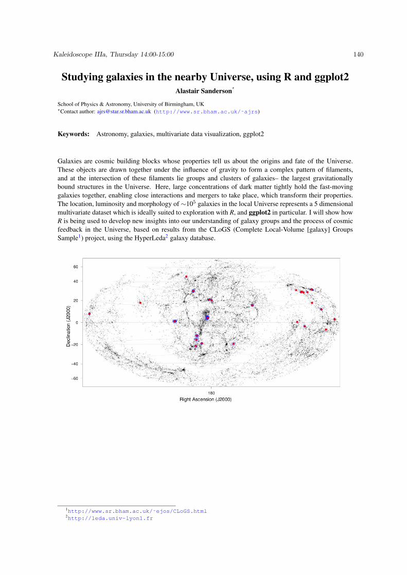
Studying galaxies in the nearby Universe, using R and ggplot2Alastair Sanderson?

School of Physics & Astronomy, University of Birmingham, UK?Contact author: [email protected] (http://www.sr.bham.ac.uk/˜ajrs)

Keywords: Astronomy, galaxies, multivariate data visualization, ggplot2

Galaxies are cosmic building blocks whose properties tell us about the origins and fate of the Universe.These objects are drawn together under the influence of gravity to form a complex pattern of filaments,and at the intersection of these filaments lie groups and clusters of galaxies– the largest gravitationallybound structures in the Universe. Here, large concentrations of dark matter tightly hold the fast-movinggalaxies together, enabling close interactions and mergers to take place, which transform their properties.The location, luminosity and morphology of ∼105 galaxies in the local Universe represents a 5 dimensionalmultivariate dataset which is ideally suited to exploration with R, and ggplot2 in particular. I will show howR is being used to develop new insights into our understanding of galaxy groups and the process of cosmicfeedback in the Universe, based on results from the CLoGS (Complete Local-Volume [galaxy] GroupsSample1) project, using the HyperLeda2 galaxy database.

1http://www.sr.bham.ac.uk/˜ejos/CLoGS.html2http://leda.univ-lyon1.fr


Panel discussion: Challenges Bringing R into Commercial

Environments Louis Bajuk-Yorgan

1,*

1. TIBCO Software Inc.


Keywords: Commercial, Applications, Panel

Champions of wider R usage within commercial environments often face multiple challenges, such as a

lack of IT knowledge or acceptance, concerns about technical support, questions around validation or

other regulatory compliance, difficulties in maintaining multiple versions of R, etc.

In this panel discussion, R champions and commercial vendors will share their views and experiences.

Questions from the audience are highly encouraged.

NOTE:

I organized a panel discussion on this topic for useR 2010. The discussion was well-attended, with lots

of questions from the audience, and several attendees approached me afterwards to suggest this be a

regular feature of useR conferences. The members of the panel from last year are listed below. If my

proposal is accepted, I would invite participation from Revolution and Mango again, and seek out new

R champions to broaden the discussion.

Panel composition last year:

- Revolution Analytics (Norman Nie, CEO)

- TIBCO (Lou Bajuk-Yorgan, Sr. Director Product Management)

- Bret Musser, Director, Clinical Biostatistics at Merck

- Mango Solutions (Richard Pugh, CTO)

- Jim Porzak, Senior Director of Marketing Analytics at Ancestry.com

- Thomas G Filloon, Principal Statistician, Procter & Gamble

Suggested logistics:

- Each speaker sends one slide to moderator (TBD), moderator controls the slides

- Each speaker has 3 minutes to talk

- Rest of the time is devoted to Q&A and discussion

Panel Discussion II, Thursday 14:00-15:00 141

microbenchmark: A package to accurately benchmark Rexpressions

Olaf Mersmann1? , Sebastian Krey1

1. TU Dortmund, Department of Statistics?Contact author: [email protected]

Keywords: Benchmarking, Timing, High Performance Computing

We present the R package microbenchmark. It provides functions to accurately measure the execution timeof R expressions. This enables the user to benchmark and compare different implementation strategies forperformance critical functions, whose execution time may be small, but which will be executed many timesin his program. In contrast to the often used system.time and replicate combination, our packageoffers the following advantages: firstly it attempts to use the most accurate method of measuring time madeavailable by the underlying operating system, secondly it estimates to overhead of the timing routines andsubtracts it from all measurements automatically and lastly it provides utility functions to quickly comparethe timing results for different expressions.

In our presentation we will first describe the implementation of the timing routines for each platform (Win-dows, MacOS X, Linux and Solaris) and highlight some of the difficulties and limitations when measuringsub-millisecond execution times. Topics covered include strategies for dealing with CPU frequency scalingand multi-core system, why elapsed time is measured and not CPU time, why time is measured and notclock cycles as well as ways to estimate the granularity of the underlying timing routine. We conclude witha practical guideline for benchmark experiments on each of the operating systems mentioned.

After the viability of timing very short running R expressions has been established, some examples areprovided to show why it is useful to study the performance characteristics of such expressions at all. Firstoff, a baseline for the “speed” of the R interpreter is established by measuring the time it takes to execute thesimplest possible function1. We consider this to be the equivalent of the cycle time of a microprocessor. Nextwe extend this idea to S3 and S4 methods to see how much overhead one incurs for the method dispatchin comparison to a simple function call. Afterwards we investigate the time it takes to generate a vectorcontaining the numbers from 1 to n (for different n) using the different methods available in base R. Timepermitting we conclude with a real world example where using high-level vectorized R functions actuallyhurt performance when compared to a naive implementation using low level operations.

1The simplest possible function being function() NULL.

Kaleidoscope IIIb, Thursday 14:00-15:00 142

Vector Image ProcessingPaul Murrell1?

1. Department of Statistics, The University of Auckland?Contact author: [email protected]

Keywords: image processing, vector graphics, importing graphics, SVG, javascript

This talk will describe a project to convert a static PDF map of a university campus into an interactive SVGmap, using R.

The conversion involves three steps: importing the original map into R, using the grImport package; pro-cessing the map contents to identify important features; and using the gridSVG package to add interactivityto the map and export it in an SVG format.

Both the import and export steps depend on some recent improvements in the handling of lines and text inthe grImport and gridSVG packages, plus the introduction of a new “path” primitive in the grid package.These new graphics features and enhancements will be described and demonstrated.

There will also be a discussion of the image processing step and the addition of interactivity to the map. Theformer will demonstrate the usefulness of treating an image as a source of data, which can be manipulatedusing the standard data processing tools in R, and the latter will demonstrate a way to add simple interactivityto the SVG output that is produced by the gridSVG package.

References

Murrell, P. gridSVG: Export grid graphics as SVG. R package version 0.6-0.

Murrell, P. (2009). Importing vector graphics: The grImport package for R. Journal of Statistical Soft-ware 30(4), 1–37.

R Development Core Team (2011). R: A Language and Environment for Statistical Computing. Vienna,Austria: R Foundation for Statistical Computing. ISBN 3-900051-07-0.

Kaleidoscope IIIb, Thursday 14:00-15:00 143

Adding direct labels to plotsToby Dylan Hocking1,2,?

1. INRIA Sierra team for machine learning research, 23 avenue d’Italie, Paris, France

2. Institut Curie/INSERM U900/Mines ParisTech cancer bioinformatics group, 26 rue d’Ulm, Paris, France?Contact author: [email protected]

Keywords: Visualization, graphics, legends, direct labels

High-level plotting systems such as lattice and ggplot2 provide automatic legends for decodingcolor labels in R plots (Sarkar, 2008; Wickham, 2009). However, with many colors, legends becomedifficult to read, and direct labels are a more suitable decoding method:

> library(lattice)

> data(mpg, package = "ggplot2")

> p <- xyplot(jitter(cty) ~ jitter(hwy), mpg, groups = class,

+ main = "City and highway fuel efficiency depends on car class")

> library(directlabels)

> print(direct.label(p))

City and highway fuel efficiency depends on car class

jitter(hwy)

jitte

r(ct

y)

10

15

20

25

30

35

20 30 40

2seater

compact

midsizeminivan

pickup

subcompact

suv

Direct labels are inherently more intuitive to decode than legends, since they are placed near therelated data. However, direct labels are not widely used because they are often much more difficultto implement than legends, and their implementation varies between plotting systems.

The directlabels package solves these problems by providing a simple, unified interface for directlabeling in R. Given a lattice or ggplot2 plot saved in the variable p, direct labels can be added bycalling direct.label(p,f) where f is a Positioning Method that describes where labels should beplaced as a function of the data. The power of this system lies in the fact that you can write yourown Positioning Methods, and that any Positioning Method can be used with any plot. So onceyou have a library of Positioning Methods, direct labeling becomes trivial and so can more easilyused as a visualization technique in everyday statistical practice.

References

Sarkar, D. (2008). Lattice: Multivariate Data Visualization with R. New York: Springer. ISBN978-0-387-75968-5.

Wickham, H. (2009). ggplot2: elegant graphics for data analysis. Springer New York.

Regular Posters 144

iRegression: a regression library to symbolic interval-valued

variables

Lima Neto Eufrásio1*, Souza Filho Cláudio1, Anjos Ulisses1

1. Departamento de Estatística, Universidade Federal da Paraíba, Cidade Universitária s/n, João Pessoa, PB, Brazil


Keywords: Regression, interval variable, symbolic data analysis.

Symbolic data analysis (SDA) has been introduced as a domain related to multivariate analysis, pattern

recognition and artificial intelligence in order to introduce new methods and to extend classical data

analysis techniques and statistical methods to symbolic data (Billard and Diday 2006). In SDA, a

variable can assume as a value an interval from, a set of real numbers, a set of categories, an ordered list

of categories or even a histogram. These new variables take into account the variability and/or

uncertainty presented in the data. Interval variables have been studied in the area of SDA, where very

often an object represents a group of individuals and the variables used to describe it need to assume a

value which express the variability inherent to the description of a group. Moreover, interval-valued

data arise in practical situations such as recording monthly interval temperatures in meteorological

stations, daily interval stock prices, among others. Nowadays, different approaches have been

introduced to analyze interval-valued variables. In the field of SDA, approaches to fit a regression

model to interval-valued data have been discussed in the literature. However, the access to such

methods still is restricted, being necessary to request to the authors. Billard and Diday (2000) were first

to propose an approach to fit a linear regression model to symbolic interval-valued data sets. Lima Neto

and De Carvalho (2008) improved the previous approach presenting a new method based on two linear

regression models, the first regression model over the midpoints of the intervals and the second one

over the ranges, which reconstruct the boundaries of the interval-values of the dependent variable in a

more efficient way when compared with the Billard and Diday's method. The aim of this work is to

development a R library, called iRegression, that includes some regression methods for interval-valued

variables. This new library will be the first one developed to treat symbolic data in the regression

context. Thus, some regression methods for symbolic interval-valued variables will be accessible to

students, teachers and professionals.

Acknowledgments : The authors would like to thank CNPq (Brazilian Agency) for their financial

support.

References Billard, L. and Diday, E. (2006). Symbolic Data Analysis: Conceptual Statistics and Data Mining, John

Wiley, New York.

Lima Neto, E.A. and De Carvalho, F.A.T.. (2008), Centre and range method to fitting a linear

regression model on symbolic interval data. Computational Statistics and Data Analysis 52, pp. 1500-

1515

Regular Posters 145

Mixtures of Unimodal DistributionsCarlos E. Rodrıguez1,2,? , Stephen G. Walker1

We present a new Bayesian mixture model. The main idea of our proposal is to change the componentsdistribution of the mixture. Whereas the normal distribution is typically used as the kernel distribution,it does have some serious issues for the modeling of clusters, see for example Escobar & West (1995) orRichardson & Green (1997). If a cluster is skewed or heavy tailed, then the normal will be inefficient andmany may be needed to model a single cluster. Our intention is to use as kernel a family of distributionfunctions for which the only constraint is that they are unimodal. Hence, we define a cluster as a set of datawhich can be adequately modeled via a unimodal distribution. To construct unimodal distributions we usea mixture of unform distributions with the Dirichlet Process, (Ferguson (1973) and Sethuraman (1994)), asthe mixing distribution. To sample from the correct posterior distribution we use the ideas of Kalli, Griffin& Walker (2009), and Damien & Walker (2001), Tierney (1994), Green (1995) and Godsill (2001).

Keywords: Unimodal Distribution, Dirichlet Process, Markov chain Monte Carlo and Slice Sampler

1. International Society for Bayesian Analysis (ISBA)2. Mexican Statistical Association (AME)?Contact author: [email protected]

References

[1] Ferguson, T. S. (1973). A Bayesian analysis of some nonparametric problems. Annals of Statistics, 1,209-230.

[2] Sethuraman, J. (1994). A constructive definition of Dirichlet priors. Statistica Sinica, 4, 639-650.

[3] Godsill, S. J. (2001). On the relationship between Markov chain Monte Carlo methods for modeluncertainty. J. Computational Graphical Statistics, 10, 230-248.

[4] Green, P. J. (1995). Reversible jump Markov chain Monte Carlo computation and Bayesian modeldetermination. Biometrika, 82, 711-732.

[5] Richardson, S. and Green, P. J. (1997). On Bayesian analysis of mixtures with an unknown number ofcomponents (with discussion). Journal of the Royal Statistical Society, Series B 59, 731-792.

[6] Escobar, M.D. and West, M. (1995) Bayesian density estimation and inference using mixtures. Journalof the American Statistical Association. 90, 577-588.

[7] Tierney, L. (1994). Markov chains for exploring posterior distributions (with discussion). Annals ofStatistics 22, 1701-1762.

[8] Damien, P. and Walker, S.G. (2001). Sampling truncated normal, beta and gamma densities. Journalof Computational and Graphical Statis- tics 10, 206-215.

[9] Kalli, M., Griffin, J.E. and Walker, S.G. (2009). Slice sampling mixture models. Statistics and Com-puting. 21, 93-105.

Regular Posters 146

Accelerating Simulations in R using Automatically Generated GPGPU-Code

Frank Kramer1*, Andreas Leha1, Tim Beissbarth1

1. Department of Medical Statistics, University Medical Center Göttingen, Göttingen, Germany*Contact author: [email protected]

Keywords: GPGPU, CUDA, Simulation, simR2CUDA

Newly developed classifiers, estimators, and other algorithms are often tested in simulations to assess power, control of alpha-level, accuracy and related quality criteria.

Depending on the required number of simulation runs and the complexity of algorithms, especially the estimation of parameters and the drawing of random numbers under certain distributions, these simulations can run for several hours or even days. Such simulations are embarrassingly parallel and, therefore, benefit massively from parallelization. Not everyone has access to clusters or grids, though, but highly parallel graphics cards suitable for general purpose computing are installed in many computers. While there is a distinct number of maintained R-packages available (Eddelbuettel2011) that are able to interface with GPUs and allow the user to speed up computations, integrating these methods in simulation runs is often complicated and mechanisms are not easily understood.

We present a new package that acts as a wrapper for CUDA-implementations and offers a systematic way for a statistician to accelerate simulations written in R. After including the package simR2CUDA the user defines the algorithm for a single simulation run in an R function and passes the function, other required parameters and the number of simulation runs to a compiler function. The allowed syntax concerning flow-control for the function defining a single simulation run is restricted to comply with GPU and implementation limitations. Given that a CUDA environment is correctly installed and configured, a wrapper function, representing the whole simulation, and a CUDA function, representing an individual simulation step, are generated and integrated into R using dyn.load. Upon calling the generated code the simulation wrapper, a simple C function, splits up the independent simulation runs for parallel execution on GPU threads and collects and returns the results, after execution of all n runs on the GPU has finished (see Figure 1).

References

Eddelbuettel (2011). CRAN Task View: High-Performance and Parallel Computing with R, http://cran.r-project.org/web/views/HighPerformanceComputing.html.

Figure 1: Illustration of generic process flow in generated code

Regular Posters 147

The State of StatETStephan Wahlbrink1, Tobias Verbeke2,?

1. WalWare / wahlbrink.eu2. OpenAnalytics BVBA?Contact author: [email protected]

Keywords: R, IDE, Eclipse, StatET, integrated development environment

The StatET plug-ins for Eclipse offer the professional R developer and statistician an integrated develop-ment environment since 2004. This presentation will look back on an interesting year of development anddemonstrate some of the hidden and less hidden new functionality that was introduced between UseR!2010and UseR!2011.

WalWare et al. (2004–2011). Eclipse Plug-In for R: StatET. http://www.walware.de/goto/statet.

Regular Posters 148

The R Service BusTobias Verbeke1,?


Keywords: R, SOA, ESB, enterprise service bus, software integration

R is a unique computational and visualization engine that can be useful to power data-driven decision makingin about any analytics problem. The complexity of many integration tasks, though, requires dedicated tools.The R Service Bus is a swiss army knife that allows you to plug R into your processes independently of thetechnology used by other software applications involved in the workflow. It has been in development forover two years and released under open source license to the R community in April 2011.

In this presentation we will provide an overview of the architecture of the R Service Bus and show how thearchitectural decisions guarantee reliability, flexibility, high availability and scalability of R-based analyticsapplications. Next we will demonstrate how applications can connect to RSB using RESTful and SOAP-based web services, e-mail protocols, messaging protocols (JMS, STOMP) etc. and which different payloadscan be used to unleash to power of R.

OpenAnalytics (2010–2011). The R Service Bus. http://www.openanalytics.eu/r-service-bus.

Regular Posters 149

Teaching Measurement Systems Analysis to Engineers Using RThomas Roth1?

The Department of Quality Science - Technical University of Berlin

?Contact author: Thomas Roth

Keywords: MSA, Capability, Gage R&R, ANOVA, DoE

Measurement Systems Analysis is an important aspect within the statistical education of engineers. Whileclassical design of experiments (DoE) is dealt with in statistical courses for engineers, more specific designsand their analysis to identify the components of variation of measurement systems are rarely discussed.These Gage Repeatability & Reproducibility studies as well as procedures relating to terms such as Bias,Linearity and Gage Capability are subject of national and international standards and obligatory within butnot restricted to automotive industry.

Methods utilizing the comprehensive qualityTools package, summaries and graphs as well as an example forteaching Measurement Systems Analysis to engineers as part of an obligatory statistics course for engineersare illustrated. The conceptual design of the methods and the relation to national and international standardsare presented.

References

A.I.A.G. (2010). Measurement systems analysis: Reference manual (4 ed.). Detroit, Mich: DaimlerChryslerand Ford Motor and General Motors.

Burdick, R. K., C. M. Borror, and D. C. Montgomery (2005). Design and analysis of gauge R&R studies:Making decisions with confidence intervals in random and mixed ANOVA models. Philadelphia, Pa,Alexandria, Va: Society for Industrial Applied Mathematics and American Statistical Association.

Herrmann, J. and T. Roth (2010). Qualitatsmanagement als Pflichtfach fur Bachelor an der TU-Berlin.In R. Schmitt (Ed.), GQW 2010 , (Aachen, Germany), // Unternehmerisches Qualitatsmanagement, pp.205–217. Aachen: Apprimus-Verl.

ISO (2008). Quality management systems – Requirements (ISO 9001:2008).

ISO (2010). Statistical methods in process management – Capability and performance – part 7: Capabilityof measurement processes (ISO 22514-7).

Roth, T. (2010). qualityTools: Statistical Methods for Quality Science.

Verband der Automobilindustrie e.V. (2010). Prufprozesseignung: Eignung von Messsystemen, Mess- undPrufprozessen, Erweiterte Messunsicherheit, Konformitatsbewertung.

Regular Posters 150

The cards PackageJason Waddell1,?


Keywords: R, cards, card games, teaching, probability

Many statistics courses use cards as examples for presenting probability theory. The cards package pro-vides tools for plotting of cards and card games, along with adaptable interactive examples for card-basedprobability exercises and games.

In this presentation we will demonstrate functions for generating randomized decks and graphically dis-playing cards. In addition we will demonstrate how the package can be used to create fully interactive cardgames (such as casino-solitaire) that record and report play statistics.

Regular Posters 151

Using R in Insurance: Examples from Lloyd’s

Markus Gesmann1,*, Viren Patel1, Gao Yu1

1. Lloyd’s, One Lime Street, London EC3M 7HA *Contact author: [email protected] Keywords: Statistical Modelling, Data Management, Financial Analysis, Graphics, R packages

We propose to present about how the Analysis team of Lloyd’s is using R in its operations. The poster focuses on 4 areas: statistical modelling, visualisation, usage of R and LaTeX to create management information, and collaboration via R packages.

Statistical modelling: Understanding the volatility of the risks insured at Lloyd’s is crucial for pricing, business planning and capital setting. The Analysis team uses R to fit loss distribution to the historical data and Monte Carlo simulation to review the performance of syndicates and the market.

Visualisation: Data visualisation can help to provide early insight into favourable or unfavourable development of the business environment. The Analysis team uses lattice and googleVis to visualize the results of our work in a form that is easy to disseminate. As an example, we introduce the Statistics Relating to Lloyd’s document, and how to use the googleVis package to display some of its information.

Using R and LaTeX to create management information: In a market with over 80 syndicates it is necessary to automatise the creation of performance reports for management information. Our team plays back Benchmarking reports which allows management and underwriters to view their own performance in the context of competitors. These reports are being produced using R and LaTex, among other software tools.

Creating internal R packages: For easier availability and dissemination teams in Lloyd’s create packages of their R functions. This includes both packages tailored to a specific task and general packages to be used to comply with internal branding guidelines.

References Lloyd’s (2010). Statistics Relating to Lloyd’s, http://www.lloyds.com/stats/.

Regular Posters 152

Solving Norm Constrained Portfolio Optimizations viaCoordinate-Wise Descent Algorithms

Yu-Min Yen1 and Tso-Jung Yen1

1. Department of Finance, LSE and Institute of Statistical Science, Academia Sinica?Contact author: [email protected]

Keywords: Portfolio optimization, norm constraint, coordinate-wise descent algorithm

In this paper we demonstrate that coordinate-wise descent algorithms can be used to solve portfolio selectionproblems in which asset weights are constrained by lq norms for 1 ≤ q ≤ 2. A special case of the suchproblems is when q = 1. The l1 norm constraint promotes zero values for the weight vector, leadingto an automatic asset selection for the portfolio. We first consider the case of minimum (global) varianceportfolio (mvp) in which the asset weights are constrained by weighted l1 and squared l2 norms. We use twobenchmark data sets to examine performances of the norm constrained portfolio. When the sample size isnot large in comparison with the number of assets, the norm constrained portfolio tends to have a lower out-of-sample portfolio variance, lower turnover rate, less numbers of active assets and short-sale positions, buthigher Sharpe ratio than the one without such norm constraints. We then show some extensions; particularlywe derive an efficient algorithm for solving an mvp problem in which assets are allowed to be chosengrouply. All of the program codes for the algorithms are written by R.

Regular Posters 153

Using R for air quality data analysis: A tool for designingimproved large-scale air pollution prevention programs

A. Alija1? , M. N. Gonzalez1, A. Junquera-Perez1, A. Ayesta1, E. Setien1, L. Garcia1 and J. Blanco1

1. Ingenieros Asesores S.A. Parque Tecnologico de Asturias. Parcela 39, 33428. Principado de Asturias


Keywords: Air quality, Air pollution, openair, data mining.

Emissions of air pollutants derive from almost all economic and societal activities. The majority of green-house gas emissions (GHG), acidifying substances, tropospheric ozone precursor emissions and materialinput caused by the life-cycles of activities related to consumption can be allocated to the main consumptionareas of eating and drinking, housing and infrastructures, and mobility [Age11].

In this work, we present an intensive use of R and more concretely package openair [CR11]. Packageopenair lead out to analyse long historical time series of air pollution data coming from a large urban regionsomewhere [pri]. Long historical series of data have the inconvenience of they are very difficult to analyzefor several reasons. Perhaps, some of these reasons are: first, air pollution data is a data extremely correlatedin time and second, air pollution data is a complex data which require a very optimized visualization toolsto carry out even the simplest analysis. Therefore, much of the data available is only briefly analysed;perhaps with the aim of comparing pollutant concentrations with national and international air quality limits.Package openair, thanks to the specific functions, helps us to overcome some of these barriers.

We would like to thanks PhD. Lucas Fernandez Seivane for our helpfull discussions.

References

[Age11] EEA (European Environment Agency). Soer2010. http://www.eea.europa.eu/soer,2011.

[CR11] David Carslaw and Karl Ropkins. openair: Open-source tools for the analysis of air pollutiondata, 2011. R package version 0.4-0.

[pri] private. To preserve the confindenciality of the data source we will keep the location anonymous.

Regular Posters 154

Invasions by polymorphic species

Elizabeth Elliott1,*

and Stephen Cornell1

1. University of Leeds


Keywords: Range-expansion; Evolution; Reaction-diffusion model; Numerical simulations

Two issues of current importance in ecology are the range expansion of species and invasion of exotic

organisms. Climate change is affecting the environments that species are currently adapted to, and to

survive species will either need to adapt to the new conditions or shift with their current environment.

Empirical observations and simulation models have shown that higher dispersal ability may lead to

increased rates of spread but little is known about the effect of having a community of dispersal

phenotypes on the rate of range expansion. We use a spatially explicit analytical model based on

partial-differential equations to investigate the invasion of a species with two dispersal phenotypes into

a previously unoccupied landscape. These phenotypes differ in both their dispersal and population

growth rate. Using analytical techniques and carrying out numerical simulations in R (R Development

Core Team, 2010) using the deSolve package (Soetaert et al., 2010), we find that the presence of both

phenotypes can result in faster range expansions than if only a single phenotype were present in the

landscape, and that typically the invasion can occur up to twice as fast as a result of this polymorphism.

This has implications for predicting species invasion speeds, suggesting that speeds cannot just be

predicted from looking at a single phenotype and that the presence of a community of phenotypes needs

to be taken into consideration.

References

R Development Core Team (2010). R: A language and environment for statistical computing. Vienna,

Austria, R Foundation for Statistical Computing.

Soetaert, K., Petzdolt, T. and Setzer, R. W (2010). Solving differential equations in R: Package

deSolve. Journal of Statistical Software 33, 1-25.

Regular Posters 155

Using R to Empower a New Plant Biology

Naim Matasci1,*, Matthew Vaughn2, Nirav Merchant1,3

1. The iPlant Collaborative, BIO5 Institute, University of Arizona 2. The iPlant Collaborative, Texas Advanced Computing Center, University of Texas at Austin. 3. Biotechnology Computing Facility, BIO5 Institute, University of Arizona *Contact author: [email protected] Keywords: cyberinfrastructure, plant sciences, bioinformatics, high performance computing The iPlant Collaborative is a U.S. National Science Foundation program to build a cyberinfrastructure for the plant sciences that will enable new conceptual advances through integrative, computational thinking. Teams composed of plant biologists and computer scientists work on grand challenges that address fundamental questions in plant biology, in particular focusing on elucidating the link between genotype and phenotype and on building a tree of life to represent the evolutionary history of all green plants. Countless computer programs address individual aspects of these grand challenges but the complexity and sheer magnitude of the problem makes it almost impossible for individual researchers or research groups to tackle such problems alone. iPlant provides a cyberinfrastructure that allows researchers in the plant science community to collaborate and share and integrate data and algorithms. Furthermore, by providing access to High Performance Computing resources it permits the generation and analysis of very large datasets as well as the usage of computationally intensive algorithms. Given the growing importance of R in virtually every field of biology and bioinformatics, iPlant’s cyberinfrastructure has been enriched by an interface to facilitate the development, execution and distribution of R scripts. Developers can work on constructing new tools in Atmosphere, iPlant’s virtual environment, through an IDE and access data and workspaces located in their iPlant home directory on in shared locations. All I/O operations are handled through iRODS, the Integrated Rule-Oriented Data System which permits the sharing of data and provides direct read access to plant genomes and other large files. The use of iRODS also ensures consistency of data across the different access point to iPlant’s cyberinfrastructure (Atmosphere, API, Discovery Environment). Through iPlant’s API users and developers can execute computationally intensive scripts on Texas Advanced Computing Center’s HPC resources. Finally, by providing a simple metadata description, developers can create GUIs for their applications and make them available to colleagues and collaborators only or to the community at large through iPlant’s Discovery Environment. References Atmosphere: http://atmo.iplantcollaborative.org/ iRODS: https://www.irods.org/ iPlant’s Discovery Environment: http://preview.iplantcollaborative.org/de/

Regular Posters 156

Rknots, an R package for the topological analysis of knottedbiological polymers

Federico Comoglio1? , Maurizio Rinaldi2

1. Department of Biosystems Science and Engineering, Swiss Federal Institute of Technology (ETH) Zurich, Basel, Switzerland2. Department of Chemical, Food, Pharmaceutical and Pharmacological Sciences (DiSCAFF), University of Piemonte Orientale

”A. Avogadro”, Novara, Italy?Contact author: [email protected]

Keywords: Rknots, knotted polymers, computational knot theory, topology, proteins

The topological study of biological polymers has led to important insights into their structural propertiesand evolution Virnau et al. (2006). From a topological point of view polymers can be naturally modeledas sequences of 3D points, i.e. open polygonal paths. Their closure generates classical objects in topologycalled knots. Boosted by Taylor’s work Taylor (2000), the characterization of knotted proteins is a subjectof increasing interest in both experimental and computational biology due to the close structure-functionrelationship and reproducible entangled folding. The exponential growth of the total number of structuresdeposited into the Protein Data Bank (PDB) requires dedicated computational high-throughput methods ableto deal with a large amount of data. These methods combine a structure reduction scheme of a protein back-bone model with the computation of a knot invariant. Being easy to compute, the Alexander polynomialrepresents the current default choice Kolesov et al. (2007). Although this choice is primarily supported bythe fact that the knots so far identified in proteins are of the simplest types, the Alexander polynomial isnot able to discern knots chirality and its limited power is not optimal to develop a generalized frameworkaiming to describe topological properties of 3D structures.Recently, we developed a topological framework for the computation of the HOMFLY polynomial Freydet al. (1985), a more powerful invariant able to define knots chirality. By screening the entire PDB, weobtained an up-to-date table of knotted proteins that also includes two newly detected right-handed trefoilknots in recently deposited protein structures Comoglio and Rinaldi (2011).However, the application of our framework is not limited to proteins and in order to provide an open-sourcepackage to the scientific community working in the field, we developed and here we present Rknots, anR package that includes functions and utilities to process and topologically explore polymers along withdedicated utilities for working with protein structures. Among the implemented functions, this first releaseincludes PDB entry import or fetching (exploiting the flexibility of the R package bio3d), structure reductionvia the Alexander-Briggs algorithm Alexander and Briggs (1926) and the MSR (Minimal Structure Reduc-tion algorithm) Comoglio and Rinaldi (2011), topological invariants and linking number computation, 3Dand knot diagram graphics function along with a knots and links dataset repository and utilities.We welcome external contributions to Rknots in order to further extend the package functionalities andprovide a general purpose tool to identify knots in three-dimensional structures.

References

Alexander, J.-W. and G.-B. Briggs (1926). On types of knotted curves. Ann of Math 28, 562–586.

Comoglio, F. and M. Rinaldi (2011). A topological framework for the computation of the homfly polynomialand its application to proteins. PLoS ONE in the press.

Freyd, P., D. Yetter, J. Hoste, W.-B.-R. Lickorish, K. Millett, and A. Ocneanu (1985). A new polynomialinvariant of knots and links. Bull Amer Math Soc (NS) 12, 239–246.

Kolesov, G., P. Virnau, M. Kardar, and L.-A. Mirny (2007). Protein knot server: detection of knots in proteinstructures. Nucleic Acid Res 35, W425–W428.

Regular Posters 157

A specialised software for statistical applications inmacromolecular crystallographyJames Foadi1,? , Gwyndaf Evans2, David Waterman3

1. MPL, Imperial College, London SW7 2AZ2. Diamond Light Source Ltd, Harwell Science and Innovation Campus, Didcot, Oxfordshire OX11 0DE3. CCP4 - Research Complex at Harwell (RCaH) - Harwell Science and Innovation Campus, Didcot, Oxfordshire OX11 0FA?Contact author: [email protected]

Keywords: Macromolecular crystallography

A new package for applications in macromolecular structural crystallography, cRy, has been developed inthe renowned R statistical platform. This is the first software of its kind and it is supposed to provide a bridgebetween the large communities of crystallographers and professional statisticians. At present macromolec-ular crystallographers make heavy use of large systems of programs, like CCP4 [1] or PHENIX [2], mainlywritten in Fortran, C/C++ or Python. These programs handle the several statistical operations, normallycarried out in crystallography, with ad hoc routines, usually developed by different authors, often not shar-ing a common statistical platform. Data and results are exchanged through files with well-defined formats.The cRy package reads and writes files in the most commonly used crystallographic formats, carries outall major crystallographic calculations and provides an interface between the crystallographic data structureand the statistical objects and tools offered by R. cRy provides, thus, that common statistical platform that,at present, is still lacking in structural crystallography. The code has been developed using S4 classes.

References

[1] Collaborative Computational Project 4 (1994). The CCP4 Suite of Programs for Protein Crystallography.Acta Cryst. D, 50, 760–763.

[2] P. D. Adams, P. V. Afonine, G. Bunkoczi, V. B. Chen, I. W. Davis, N. Echoo Is, J. J. Headd, L. -W.Hung, G. J. Kapral, R. W. Grosse-Kuntsleve, A. J. Terwilliger and P. H. Zwart (2010). PHENIX: acomprehensive Python-based system for macromolecular structure solution. Acta Cryst. D, 66, 213–221.

Regular Posters 158

EMA - A R package for Easy Microarray data AnalysisNicolas Servant1,2,3,?, Eleonore Gravier1,2,3,4,, Pierre Gestraud1,2,3, Cecile Laurent1,2,3,6,7,8, CarolinePaccard1,2,3, Anne Biton1,2,3,5, Isabel Brito1,2,3, Jonas Mandel1,2,3, Bernard Asselain1,2,3, Emmanuel

Barillot1,2,3, Philippe Hupe1,2,3,5

1. Institut Curie, Paris F-75248, France2. INSERM, U900, Paris F-75248, France3. Ecole des Mines ParisTech, Fontainebleau, F-77300 France4. Institut Curie, Departement de Transfert, Paris F-75248, France5. CNRS, UMR144, Paris F-75248, France6. CNRS, UMR3347, Orsay F-91405, France7. INSERM, U1021, Orsay F-91405, France8. Universite Paris-Sud 11, Orsay F-91405, France?Contact author: [email protected]

Keywords: Microarray analysis

The increasing number of methodologies and tools currently available to analyse gene expression microar-ray data can be confusing for non specialist users. Based on the experience of biostatisticians of InstitutCurie, we propose both a clear analysis strategy and a selection of tools to investigate microarray gene ex-pression data. The most usual and relevant existing R functions were discussed, validated and gathered inan easy-to-use R package (EMA) devoted to gene expression microarray analysis.Removing noise and systematic biases is performed using the most famous techniques for AffymetrixGeneChip normalisation. The data are then filtered to both reduce the noise and increase the statisticalpower of the subsequent analysis. Exploratory approaches based on R packages such as FactoMineR, ormostclust and classically used to find clusters of genes (or samples) with similar profiles are also offered.Supervised approaches, as Significance Analysis of Microarrays (siggenes package) approach or ANOVAfunctions, are proposed to identify differentially expressed genes (DEG) and functional enrichment of theDEG list is assessed based on GOstat package.The package includes a vignette which describes the detailed biological/clinical analysis strategy used atInstitut Curie. Most of the functions were improved for ease of use (fewer command lines, default parame-ters tested and chosen to be optimal). Relevant, enhanced and easy-to-interpret text and graphic outputs areoffered. The package is available on The Comprehensive R Archive Network repository.

References

Bertoni, A. and G. Valentini (2007). Model order selection for bio-molecular data clustering. BMC Bioin-formatics 8 Suppl 2, S7.

Falcon, S. and R. Gentleman (2007). Using GOstats to test gene lists for GO term association. Bioinformat-ics 23, 257–258.

Le, S., J. Josse, and F. Husson (2008). Factominer: an R package for multivariate analysis. Journal ofstatistical software 25, 1–18.

Servant, N., G. Eleonore, P. Gestraud, C. Laurent, C. Paccard, A. Biton, I. Brito, J. Mandel, B. Asselain,E. Barillot, and P. Hupe (2010). Ema - a R package for easy microarray data analysis. BMC ResearchNotes 3, 277.

Tusher, V. G., R. Tibshirani, and G. Chu (2001). Significance analysis of microarrays applied to the ionizingradiation response. Proc Natl Acad Sci U S A 98, 5116–21.

Regular Posters 159

Classification of Enzymes via Machine Learning Approaches

Neetika Nath*, John B. O. Mitchell

Biomedical Sciences Research Complex and School of Chemistry, University of St Andrews, KY16 9ST*[email protected]

Keywords: Enzyme Classification, Machine Learning, R, Protein Function Prediction.

Abstract: We compare enzyme mechanistic descriptors derived from the MACiE (Mechanism,

Annotation and Classification in Enzymes) database [Holliday et al., 2006] and use multivariate

statistical analysis for assessment of enzyme classification. Each enzyme has an Enzyme Commission

(EC) number, a numerical code designed to classify enzymes by describing the overall chemistry of

the enzymatic reaction. The EC number system was devised five decades ago, in a pre-bioinformatics

age. As the volume of available information is increasing, a large number of informatics groups have

tried to use protein sequence and structural information to understand and reproduce the classification,

some of which have been successful [Cai et al., 2004]. Other groups have effected automatic EC

classification using chemoinformatics descriptions of the underlying reactions. Our objective is to

develop a computational protocol using the R package CARET [Kuhun et al., 2007] to predict EC

number from MACiE-derived descriptors. We evaluate 260 well annotated chemical reaction

mechanisms of enzymes using machine learning methods, placing them into the six top level EC

classes. Moreover, we compare the classification performances of three supervised learning

techniques, Support Vector Machine (SVM) [Vapnik, 1998], Random Forest (RF) [Breiman, 2001]

and K Nearest Neighbour (kNN), for the reaction mechanism classification task using five different

descriptor sets from MACiE data. Results: We found that all classifiers performed similarly in terms

of overall accuracy with the exception of K Nearest Neighbour analysis, which has the lowest

performance. The best performance was achieved by the Random Forest classifier.

References

Holliday, G.L., et al.. (2006) MACiE (Mechanism, Annotation and Classification in Enzymes): noveltools for searching catalytic mechanisms http://www.ebi.ac.uk/thornton-srv/databases/MACiE/

Cai, C., L. Han, et al. (2004). "Enzyme family classification by support vector machines." Proteins55: 66 - 76.

Kuhn, M., Wing, J., Weston, S, Williams A., Keefer, C. & Engelhardt, A. (2007) caret: Classificationand Regression Training, http://cran.r-project.org/web/packages/caret/

Vapnik, V. N. (1998) Statistical Learning Theory. New York: John Wiley and Sons.

Breiman, L. (2001) “Random forests,” Machine Learning, vol. 45, no. 1, pp. 5– 32.

Regular Posters 160

BeadDataPackR: A Compression Tool For Raw IlluminaMicroarray Data

Mike L. Smith1,? , Andy G. Lynch1

1. Department of Oncology, University of Cambridge, Cancer Research UK Cambridge Research Institute, Robinson Way, Cam-

bridge CB2 0RE, UK?Contact author: [email protected]

Keywords: Bioinformatics, Microarray, Illumina, Compression

Microarray technologies have been an increasingly important tool in biological research in the last decade,and a number of initiatives have sought to stress the importance of the provision and sharing of raw microar-ray data. Illumina BeadArrays provide a particular problem in this regard, as their random construction andhigh number of replicate probes simultaneously adds value to analysis of the raw data and obstructs the shar-ing of those data, with many of the standard repositories having no facilities for storing the raw data. Thisleaves the burden of distributing such data with the individual researcher. The BeadDataPackR packageprovides an interface to a novel compression scheme for raw Illumina BeadArray data, designed to ease thestorage and bandwith concerns that providing access to such data brings. It offers two key advantages overoff-the-peg compression tools. First it uses knowledge of the data formats to achieve greater compressionthan other approaches, and second it does not need to be decompressed for analysis, but rather the valuesheld within can be directly accessed by existing tools, such as the popular beadarray package.

References

M.L.Smith and A.G.Lynch (2010). BeadDataPackR: A Tool to Facilitate the Sharing of Raw Data fromIllumina BeadArray Studies. Cancer Informatics 9, 217–227.

Regular Posters 161

GWAtoolbox: An R Package for Time Efficient Quality Controlof Multiple GWAS Data Files

Daniel Taliun1,2,? , Christian Fuchsberger3, Peter P. Pramstaller1, Cristian Pattaro1 on behalf of theCKDGen consortium

1. Institute of Genetic Medicine, European Academy Bozen-Bolzano (EURAC), Bolzano, Italy2. Free University of Bozen-Bolzano, Bolzano, Italy3. Department of Biostatistics, University of Michigan, Ann Arbor, MI?Contact author: [email protected]

Keywords: genome-wide association study, quality control, visualization

In the recent years, Genome-Wide Association Studies (GWASs) have been proven to be a very powerfulapproach to uncover common genetic variants affecting human disease risk and quantitative outcome levels.To date, 1212 genetic loci were reported to be significantly associated with at least one of 210 traits (Hin-dorff et al. (2011)). To allow sufficient power to identify variants with small effects, GWAS sample sizehas been augmented by pooling results from dozens of individual GWASs into large meta-analyses efforts.However, combining results from a large number of GWASs, which differ in terms of study design, popula-tion structure, data management, and statistical analysis, poses several challenges regarding the consistencyand quality of data which are usually difficult to be addressed systematically. This is mainly due to theGWAS file size, which typically includes 2.5 to 7 million rows (corresponding to genetic variants) and > 9columns (attributes). Consequently, the data harmonization across studies usually takes several weeks ormonths.

While working in the CKDGen Consortium, aim to detect renal function genes (Kottgen et al. (2010)), wehave been performing meta-analyses of several GWASs. To standardize and speed up the quality control(QC) process we developed the GWAtoolbox, an R package which lightens and accelerates the handling ofhuge amounts of data from GWASs. GWAtoolbox provides time efficient QC of data stored in dozens offiles. Based on a simple configuration script, GWAtoolbox can process any number of files and produceQC reports in a matter of minutes. QC reports consist of an extensive list of quality statistics and graphicaloutput presented using DHTML, which allow fast and easy inspection of individual data files. Additionalstatistics and graphs allow quick identification of studies that are systematically different from the other(outliers). The high time efficiency was achieved through the data reduction technique integrated into thevisualization pipeline. In particular, instead of passing all the million data points to the R plotting routines,only a small part of data points is selected in a such way that preserves the quality of the final graphicaloutput. Additionally, the implementation of all computationally intensive steps was transferred to C++.

Through its extensive use in several current GWAS meta-analyses, GWAtoolbox has been proven to sig-nificantly speed up the data management and to improve the overall meta-analysis quality. GWAtoolbox isopen source and available for MacOS, Linux, and Windows OS, at http://www.eurac.edu/gwatoolbox.

References

Hindorff, L. et al. (2011). A catalog of published genome-wide association studies. Available at:www.genome.gov/gwastudies. Accessed March 23, 2011.

Kottgen, A. et al. (2010). New loci associated with kidney function and chronic kidney disease. NatGenet 42(5), 376–84.

Regular Posters 162

Is the seasonal variation in hospitalisations rates of atrialfibrillation induced strokes in Denmark and New Zealand

dynamic?Anette Luther Christensen1,? , Simon Hales2, Sren Lundbye-Christensen1, Lars HVilsted

Rasmussen1, Kim Overvad1, Claus Dethlefsen1

1. Department of Cardiology, Center of Cardiovascular Research, Aalborg Hospital, Aarhus University Hospital, Aalborg, Denmark2. Department of Public Health, University of Otago, Wellington, New Zealand?Contact author: [email protected]

Keywords: State space model, Model selection, Seasonal variation, Atrial Fibrillation, Stroke

Atrial Fibrilation (AF) is the most common cardiac arrythmia Friberg et al. (2003) and the hospitalisationsrates of AF have increased during the last two decades; in fact AF is considered an epidemic. The frequencyof AF increases with age and considering the population demographic it is expected that the number ofpeople with AF will be increasing remarkably. Having AF often leads to palpitations, respiratory distress,and fatigue. Furthermore, AF is considered an independent risk factor for stroke Wolf et al. (1991). Theconsequences of stroke on patients are crucial and may be a considerable burden on society regarding reha-bilitation of stroke patients. It has been reported that hospitalisations with stroke exhibit seasonal variationduring the calendar year, however seasonal variations in AF induced strokes have not been investigated.Furthermore, it has not been investigated whether there has been changes in the seasonal variation of strokehospitalisations. Knowledge of the seasonal variation of AF induced stroke, and possible changes over time,may contribute to knowledge of the etiology of AF and may improve prophylaxis treatment in AF patients,which may lead to improved prognoses for AF patients.

Using a state space model to fit daily incidence rates of AF induced strokes, accounting for a secular trendand modelling the seasonal variation as a sum of sinusoids with different frequencies, it is possible to inves-tigate whether hospitalisations of AF induced strokes exhibit seasonal variation. Furthermore, performingmodel selection we may be able to investigate the dynamic nature of the seasonal variation over time. How-ever, modelling the daily incidence rates of AF induced strokes as being Poisson distributed using a statespace model, as proposed by Lundbye-Christensen et al. Lundbye-Christensen et al. (2009), is not trivial inregards to estimation algorithms and especially performing model selection.

We identified daily hospitalisations in Denmark using the Danish National Patients Registry, and in NewZealand using the National Minimum Data Set. Both registries hold records of all hospitalisations, eachrecord includes information on date of hospitalisation and primary diagnosis as well as secondary diagnoses.Analyses will be performed on data sets from each country separately, to make comparisons of seasonalvariation in incidence rates of AF induced strokes between the two countries. All analyses will be performedin R using the package sspir.

References

Friberg, J., P. Buch, H. Scharling, N. Gadsbll, and G. B. Jensen (2003). Rates of Hospital Admissions forAtrial Fibrillation. Epidemiology 13(6), 666–672.

Lundbye-Christensen, S., C. Dethlefsen, A. Gorst-Rasmussen, T. Fischer, H. C. Schønheyder, K. J. Roth-man, and H. T. Sørensen (2009). Examing Secular Trends and Seasonality in Count Data Using DynamicGeneralized Linear Models: a New Methodological Approach Illustrated with Hospital Discharge Dataon Myocardial Infarction. European Journal of Epidemiology 24(5), 225–230.

Wolf, P. A., R. D. Abbott, and W. B. Kannel (1991). Atrial Fibrillation as an Independent Risk Factor forStroke: the Framingham Study. Stroke 22(8), 983–988.

Regular Posters 163

Predictive Tool Development

A Time-to-event study of Diabetes Complications in Ontario

Kelvin Lam

1*, Douglas Manuel

1,2

1. Institute for Clinical Evaluative Sciences, Toronto, Ontario, Canada

2. The Ottawa Hospital Research Institute, Ottawa, Ontario, Canada

* Contact author : [email protected]

Keywords: Diabetes Complications, Competing Risk, Data Visualization, Administrative

Database, Diagnostic Tools

For physicians and people with diabetes, a simple and accurate predictive tool for

complications such as acute myocardial infarction (AMI) and cardiovascular disease (CVD)

will be invaluable for clinical decision making. Our study looked at how age and previous

medical history affects duration to these complications as well as death using the competing

risk methodology, where the latter served as the main competing event. R package cmprsk

was used to derive model parameters and baseline cumulative hazards. To determine the

model validity, diagnostics including c-index, deciles plots and quantile risk ratio plots will be

presented using ggplot2.

References

[1] Fine JP and Gray RJ (1999) A proportional hazards model for the subdistribution of a

competing risk. JASA 94:496-509.

[2] Putter H, Fiocco M, Geskus RB (2007). Tutorial in biostatistics: Competing risks and

multi-state models. Statistics in Medicine 26, 2389–2430.

[3] Bob Gray <[email protected]> (2010). cmprsk: Subdistribution Analysis of

Competing Risks. R package version 2.2-1. http://CRAN.R-project.org/package=cmprsk

Regular Posters 164

Analyzing the American Community Survey with R

Anthony Damico1,* , Rachel Licata1

1. Kaiser Family Foundation *Contact author: [email protected] Topic Area: Statistics in the Social and Political Sciences Keywords: American Community Survey, Health Policy, Big Data, SQL, County‐Level Data Research Objective: Designed to replace the information gathered by the decennial Census, the American

Community Survey (ACS) is likely to play an increasingly important role in the future of health policy research,

especially for regional and state‐level studies. Despite powerful statistical analysis, data manipulation, and

presentation capabilities, the open‐source R Statistical Software Package has not become widely adopted in the

fields of health economics, health policy, or healthcare management and evaluation. User guidelines and other

technical documents for government‐funded and publicly‐available data sets rarely provide appropriate syntax

examples to R users. The objective of this presentation will be to describe the steps required to import ACS data

into R, to prepare that data for analysis using the replicate weight variance and generalized variance formula

calculation techniques, and to produce the principal set of statistical estimates sought by health policy

researchers.

Study Design: This presentation reviews the step‐by‐step method explanations and syntax needed to analyze the

ACS with the R Statistical Software package. This includes importation instructions, estimate calculations,

variance and error term calculations, as well as linkages to other data sets. In order to equip healthcare

researchers with the tools needed to analyze this large dataset on their personal computers, each of these steps

include a brief discussion of absolute minimum computing requirements, as well as detailed workarounds and

shortcuts for the more memory‐intensive processes.

Population Studied: The ACS represents all civilian, noninstitutionalized Americans. The examples used in this

presentation include state and regional estimates; however, all instructions and syntax are presented with the

intention of allowing the researcher to re‐define a population of interest with minimal effort.

Principal Findings: Depending on research budget, computing resources, and level of programming skill,

conducting analyses of the ACS with R often presents a viable alternative to other statistical analysis packages.

Conclusions: Given the large file size of the ACS, interested health policy researchers may be limited in their

ability to analyze this survey with off‐the‐shelf statistical software packages due to memory overload issues.

Although R users often experience similar memory limits and problems, the flexibility of the core R programming

language and its integration with both parallel processing engines and Structured Query Language (SQL) allows

for the relatively straightforward analysis of large, complex‐sample survey data such as the ACS.

Implications for Policy, Practice or Delivery: Providing health policy researchers and statisticians with a strategy

to work with the American Community Survey using freely available software will increase their ability to

examine a variety of health and demographic indicators at the sub‐national level. By outlining the technical

steps to analyze this data, researchers could study topics such as regional characteristics of Health Professional

Shortage Areas, state demographic factors associated with Medicare Advantage plan premiums, or county‐level

demographics of uninsured populations. An understanding of the methods needed to work with the ACS will

open up the field of geographic region‐based analyses to health policy researchers.

Regular Posters 165

Nonparametric estimation of a heaping mechanism for preciseand heaped self-report data

Sandra D. Griffith1,? , Saul Shiffman2, Daniel F. Heitjan1

1. Department of Biostatistics & Epidemiology, University of Pennsylvania2. Department of Psychology, University of Pittsburgh?Contact author: [email protected]

Keywords: Digit preference, Coarse data, Rounded data, Smoking cessation, Measurement error

Open-ended numerical measures, often used in self-report to assess quantities or frequencies, exhibit a formof measurement error termed heaping. Heaping occurs when quantities are reported with varying levelsof precision. Digit preference is a special case of heaping where the preferred values are round numbers.Daily cigarette counts, for example, commonly exhibit heaps at multiples of 20, and to a lesser extent, 2, 5,and 10, when measured by retrospective recall methods. Because heaping can introduce substantial bias toestimates, conclusions drawn from data subject to heaping are suspect. Several methods have been proposedto estimate the true underlying distribution from heaped data, but all depend on unverifiable assumptionsabout the heaping mechanism. A data set in which subjects reported cigarette consumption by both a precisemethod (ecological momentary assessment as implemented with a hand-held electronic device) and a moretraditional, imprecise method (timeline followback, or periodic retrospective recall) motivates our method.We propose a nonparametric method to estimate the conditional distribution of the heaping mechanism giventhe precise measurement. We measure uncertainty in the heaping mechanism with a bootstrap approach. Wedescribe our implementation of the method using R and graphically illustrate our results with the ggplot2package. Application to our data suggests that recall errors are a more important source of bias than actualheaping.

References

Griffith, S. D., S. Shiffman, and D. F. Heitjan (2009, November). A method comparison study of timelinefollowback and ecological momentary assessment of daily cigarette consumption. Nicotine & tobaccoresearch 11(11), 1368–73.

Shiffman, S. (2009, September). How many cigarettes did you smoke? Assessing cigarette consumption byglobal report, Time-Line Follow-Back, and ecological momentary assessment. Health psychology 28(5),519–26.

Wang, H. and D. F. Heitjan (2008, August). Modeling heaping in self-reported cigarette counts. Statisticsin medicine 27(19), 3789–804.

Regular Posters 166

Forecasting multivariate time series using the DLM package:An application to road traffic networks

Osvaldo Anacleto-Junior

Dept. of Mathematics and Statistics, The Open University, Milton Keynes, UKContact author: [email protected]

Keywords: DLM package, traffic networks, time series, graphical models

Traffic data have some characteristics that can be quite challenging to deal with from a statistical modellingperspective. To have a broad view of the traffic network under analysis, information have to be collectedfrom a series of sites, which can generate a high-dimensional multivariate time series. Also, as managementdecisions have to be taken in real time during periods like rush hours, traffic systems require forecasts in aon-line environment.

Traffic flows in a road network can be modelled by a class of models known as graphical dynamic models.These models use a directed acyclic graph (DAG) in which the nodes represent the time series of trafficflows at the various data collection sites in a network, and the links between nodes represent the conditionalindependence and causal structure between flows at different sites. The DAG breaks the multivariate modelinto simpler univariate components, each one being a dynamic linear model (DLM). This makes the modelcomputationally simple, no matter how complex the traffic network is, and allows the forecasting model towork in real-time. Also, graphical dynamic models can accommodate changes that may happen in a networkdue to external events like traffic accidents and roadworks, which can heavily affect traffic flows and alsothe structure of the network, leading to sudden changes in the data being analysed.

This poster will report an application of this class of model using the DLM package in a busy motorwayjunction in the UK. It will be shown the advantage of some package features over standard DLM modelfitting approaches, focusing in particular on its numerically stable singular value decomposition-based al-gorithms implemented for filtering.

Regular Posters 167

Who’s in the Waiting Room? Modelling Multivariate TimeSeries of Counts of Patients to Hospital Emergency

DepartmentsSarah Bolt1,? , Ross Sparks1, James Lind2

1. CSIRO Mathematics, Informatics and Statistics, North Ryde, NSW, Australia2. Gold Coast Hospital, Southport, QLD, Australia?Contact author: [email protected]

Keywords: Multivariate, Times Series, Health Informatics.

While predictive tools are already being implemented to assist in forecasting the total volume of patients toEmergency Departments [Jessup et al. (2010)], early detection of any changes in the types of patients presentingwould help authorities to manage limited health resources and communicate effectively about risk, both ina timely fashion. But before we are able to detect changes we must understand and model the expectedcounts of presentations for all possible subgroups. For example, we need to forecast the expected numberof patients on a given day at a particular hospital, with a particular disease, of a particular age, sex, etc.

So our objective was to model this large collection of interdependent time series. This problem presenteda number of issues including the sheer number of them and the fact that many of these time series hadvery low counts and displayed overdispersion relative to a Poisson model. Furthermore, since the goal ofthese models was to model away known behaviours, we had to incorporate effects including significantseasonality, day of the week effects and some strongly interacting variables.

The method we present here divided the problem into two different components. The first used a regressionapproach to model time series of aggregated counts. The second allocated proportions of these counts tosubgroups using a binary regression tree analysis. This method thus drew together R functionality from twodifferent areas:

• Analysis of times series of counts using glm stats [R Development Core Team (2010)], glm.nb MASS[Venables and Ripley (2002)] and gamlss gamlss [Rigby and Stasinopoulos (2005)]. The latter function al-lowed us to model counts with a negative binomial distribution and a modelled dispersion parameter.

• Allocation of counts to subgroups using the poisson regression tree approach of rpart rpart[Therneau et al. (2010)].

References

Jessup, M., M. Wallis, J. Boyle, J. Crilly, J. Lind, D. Green, P. Miller, and G. Fitzgerald (2010). Imple-menting an emergency department patient admission predictive tool. Journal of Health Organization andManagement 24, 306–318.

R Development Core Team (2010). R: A Language and Environment for Statistical Computing. Vienna,Austria: R Foundation for Statistical Computing. ISBN 3-900051-07-0.

Rigby, R. A. and D. M. Stasinopoulos (2005). Generalized additive models for location, scale andshape,(with discussion). Applied Statistics 54, 507–554.

Therneau, T. M., B. Atkinson, and B. D. Ripley. (2010). rpart: Recursive Partitioning. R package version3.1-48.

Venables, W. N. and B. D. Ripley (2002). Modern Applied Statistics with S (Fourth ed.). New York:Springer. ISBN 0-387-95457-0.

Regular Posters 168

Algorithm for defining hospital stays

Katrine Damgaard1*

, Jon Helgeland1,

1. Norwegian Knowledge Centre for the Health Services


Keywords: Healthcare, hospitals, Multicore

Objective: The objective was to link hospital stays which constituted a complete chain of admissions

for patients transferred between wards/department within/between hospitals, in order to compare

mortality between hospitals

Material and methods: The Norwegian Knowledge Centre for the Health Services has developed a

system for retrieving data from the patient administrative systems (PAS) at all Norwegian hospitals.

By use of this system, we retrieved PAS data from each hospital for patients discharged during 2005-

2009.

Each record corresponds to one admission at one ward within a department in a hospital. To define a

complete patient stay, we have to aggregate the admissions; stays at one department, hospital stays and

stays involving more than one hospital. The latter is important for patients transferred between

hospitals to obtain their complete medical treatment history. All permanent residents in Norway have a

personal identification number (PIN) which enables linking between hospitals.

We have developed an algorithm that concatenates the ward admissions to a chain of admissions. The

function gives you all the levels of stays described above. The input to the function is a serial number,

PIN, date of admission, date of discharge, hospital, department and further optional parameters. The

function uses the package multicore in R, for the ability to use more than one processor for large

datasets. One of the properties of the algorithm is that you can choose different time windows, or

tolerances, for concatenating the ward admissions. We chose 24 hours as tolerance for our purpose.

Results: With the choice of 24 hours time window for difference between time of discharge and next

admission, we found 10 485 022 hospital stays involving one or more hospitals out of 16 370 163

ward admissions from 3 304 546 patients.

Conclusion: The algorithm can be used to aggregate large patient administrative data sets, with

acceptable running times. The tolerance limit can be adjusted to suit the purpose and the data at hand.

Regular Posters 169

Using merror 2.0 to Determine Measurement Bias and Imprecision

Richard A. Bilonick1,2,*

1. University of Pittsburgh School of Medicine, Dept. of Ophthalmology2. University of Pittsburgh Graduate School of Public Health, Dept. of Biostatistics*Contact author: [email protected]

Keywords: Measurement Error, Calibration, Bias, Imprecision, Grubbs' Estimator

Researchers often need to evaluate the agreement between n=2 or more devices (instruments, methods) based on measurements made jointly on N items (subjects). In the simplest case, each

measurement X ij for device i and item j is described as:

X ij=ii jij

where i and i describe how device i distorts (biases) the unknown true values j , and ij is a

Normally distributed random error with mean 0 and standard deviation (SD) i for device i. could

be distributed Normally with mean and SD in some applications. For uniqueness, the geometric

average of all of the i is constrained to equal one. Jaech (1985) describes many approaches to

estimating the parameters including method of moments (MOM) and maximum likelihood (ML). Estimates of these parameters will provide calibration curves relating any two devices, for example.

For simple cases of 3 or more devices and only one measurement from each device, the merror package provides several useful functions. ncb.od (non-constant bias - original data) computes ML

estimates of the bias and imprecision parameters based on the N×n rectangular array of measurements. You must have at least n=3 devices (or independently repeat at least 1 of two devices) because otherwise there is not enough information to compute all the parameter estimates uniquely (without making very strong assumptions about the parameters). Essentially, ncb.od fits a

measurement error structural equation model with just one latent variable (for ). ncb.od will

compute estimates of the i , i , i for each device, and (with confidence intervals for the i

and ). You should be aware, however, that only certain functions have meaning: 1) when the i do

not all equal 1, then you need the ratios of the i to check for scale bias (devices have different sized

measurement units, i.e., a non-constant bias or bias that changes with the level of the true value), 2)

when the i all equal 1, then differences among the i estimate constant relative biases, and 3) the

device imprecision i must be divided by the corresponding i in order to be compared (otherwise,

you are dealing with incomparable results from different measuring systems). Also included is the

function lrt to do likelihood ratio tests of the i . To visualize the data, use pairs.me to make

modified pairs plots where all the axis limits are the same for all plots with the line of equality (no

bias) indicated. Finally, precision.grubbs.cb.pd and precision.grubbs.ncb.od are

provided to compute estimates of the imprecision SD's based on, respectively, using paired data under the constant bias model, and using the original data under the non-constant bias model. To implement these functions, the Fortran code from Jaech (1985) was translated to R. Some minor computational mistakes in the Fortran code were fixed when re-writing in the R programming language.

References

Jaech, J. L. (1985). Statistical Analysis of Measurement Errors, John Wiley & Sons, New York.


Using Metabolomics to monitoring kidney transplanted patients: transplant from a living donor.

M. Calderisi1 , A. Vivi1 , M. Tassini1 , M. Carmellini2

1. NMR Centre University of Siena, Italy 2. Department of Surgery and Bioengineering, University of Siena, Italy *Contact author: [email protected] The work was partially supported by Consorzio Interuniversitario Trapianti d'Organo (www.consorziotrapianti.it) Keywords: metabolomics, chemometrics, transplant, living donor, NMR

NMR spectroscopy is a analytical platform for biological matrices, it enables the quick generation of spectral profiles of low molecular weights metabolites. Metabonomics is a system approach used also to investigate the metabolic profile by multivariate data analysis tools. The aim of the work is to control the kidney graft recovery process in an non-invasive way, estimating the process by 1H-NMR spectroscopy and chemometrics on urine samples as they contains metabolites concerning the pathological and clinical state of the patients. The goal of this statistical analysis is the identification of the dynamic biopatterns (individual patient recovery trajectories) related to the transplant. Samples have been collected every day, for both patients, along all the recovery period. The donor is a 60 years old healthy woman (6 samples), the recipient is his son, a 31 years old man (10 samples).

Data have been pre-processed (baseline correction, spectra alignment, water signal exclusion and normalization to unit length) and pre-treated (mean centering and log10 transformation). The log10 transformation has been especially useful to reduce the natural difference between high-intensity and low-intensity peaks, without boosting noise. Data have been analyzed by means of PCA and significant signal regions have been identified by selection of the highest loadings (in absolute value).

The scores plot in figure clearly shows the difference between the metabolic profile before (right side) and after (left side) the surgery (that happen during day 3) for recipient (ric) and his recovery trajectory occurring from day 5 to day 10. The metabolic profile of the donor (don) goes from a "normal" state (bottom right of the scores plot) to an altered state (top right) after the surgery day, then goes back to its original condition.

In conclusion, it is possible to state that NMR spectra plus chemometrics elaboration could be used to monitor a kidney graft recovery progress. Data elaboration has been carried out using FactoMiner and ptw and packages.

References Francois Husson, Julie Josse, Sebastien Le and Jeremy Mazet (2010). FactoMineR: Multivariate

Exploratory Data Analysis and Data Mining with R. R package version 1.14. http://CRAN.R-project.org/package=FactoMineR

Bloemberg, T. G. et al. (2010) "Improved Parametric Time Warping for Proteomics", Chemometrics

and Intelligent Laboratory Systems, 104 (1), 65-74


hyperSpecGUI:Graphical Interaction in Spectroscopic Data Analysis

Sebastian Mellor1, Claudia Beleites2,? , Colin Gillespie1, Christoph Krafft2, and Jurgen Popp2,3

1. School of Mathematics & Statistics, Newcastle University, Newcastle/UK.2. Institute of Photonic Technology, Jena/Germany.3. Institute of Physical Chemistry and Abbe Center of Photonics, University Jena/Germany.?Corresponding author: [email protected]

Keywords: spectroscopy; Google Summer of Code; GUI.

Spectroscopic data analysis includes highly visual tasks that need graphical user interaction. We presenthyperSpecGUI, a companion package enhancing hyperSpec. Both packages are hosted at hyperspec.r-forge.r-project.org.

The hyperSpecGUI packages follows the “specialise on a single thing” paradigm, as opposed to implement-ing an integrated development environment (IDE) or all-(spectroscopic)-purpose GUI. Visual interaction isprovided by small, specialised GUIs (applets, dialogs) that are called as functions. This allows full GUIinteraction with scripts and easy integration with IDEs. In particular, this allows:

Fast work-flow creation: rather than a single GUI, we use a combination of small, bespoke GUIs.

Flexibility: the package is extensible and easily adapted to new and unforeseen tasks.

Compatibility with batch processing: spectroscopic data sets are large with data analysis often includinghigh performance computations on remote servers that do not provide graphical interaction. Swappingbetween GUI-based and command line based work/batch processing are smooth and easy.

Reproducibility: interactive tasks can be recorded, allowing literate programming techniques to be used,e.g. Sweave.

Interactive spike correction of Raman spectra: when cosmic rays hit the detector, spikes are observed inthe Raman spectra. Several strategies to identify these artifacts exist and work well with high, sharp spikes.However, manual control and adjustment of the results is necessary as broader artifacts may be confusedwith sharp Raman bands and vice versa. Also the borders of broader artifacts are difficult to detect.

As an example, we present a GUI for spike filtering of Raman data, demonstrating the wrapping of this GUIwith existing IDEs/editors.

Acknowledgements. SM’s work is funded by the Google Summer of Code 2011. CB, CK, and JP acknowl-edge funding by the European Union via the Europaischer Fonds fur Regionale Entwicklung (EFRE) andthe “Thuringer Ministerium fur Bildung, Wissenschaft und Kultur” (Project: B714-07037).


Visualisation for three-dimensional shape dataStanislav Katina1,? and Adrian Bowman1

1. School of Mathematics and Statistics, The University of Glasgow, University Gardens, Glasgow G12 8QQ, Scotland, UK?Contact author:[email protected][Late Breaking Poster Abstract, topic: Visualization & Graphics ]

Keywords: Procrustes shape coordinates, thin-plate splines, 3D facial surfaces, shape index

In Late Breaking Poster we present visualisation of shape-space Principal Component Analysis (PCA)of (semi)landmarks from 3D facial surfaces. This multivariate model decomposes shape signal into low-dimensional linear combinations of high-dimensional measurements. Using Generalized Procrustes Analy-sis (Bookstein 1991), Procrustes Shape Coordinates (PSC) are calculated after suitable re-scaling, transla-tion, and rotation of the data and then decomposed to affine and non-affine components. PCA is performedby singular value decomposition of the covariance matrix of centered PSC.

The data consists of 3D coordinates of23 landmarks and1664 semilandmarks on curves and surface patchestaken from facial surfaces. Then, suitably scaled eigenvectors of the covariance matrix mentioned abovewere added to the symmetrised mean (reference shape) calculated by relabeling and reflecting the meanshape (semi)landmark coordinates. Using a carefully chosen mesh of59242 points triangulated by117386faces and derived1694 (semi)landmarks, we calculated standardized mesh points of the reference shape(called Thin-Plate Spline morph) by TPS interpolation model. This process is performed in an anatomicallyand geometrically meaningful manner, similar to the dense correspondence model of Mao et al. (2006)where the sum of principal curvatures is equivalent to bending energies. To explore the nature of particularPCs, we visualised 4D maps of signed pointwise Euclidean distances (in the sense of inwards/outwardsfacial direction) between shapes equivalent to extremes of the PC scores. Furthermore, these distanceswere decomposed tox, y, andz components of a suitably oriented face. Additionally, a shape index (SI)was calculated from principal curvatures derived from the Weingarten curvature matrix as a function ofcoefficients of a locally fitted parabolic regression model to facial coordinates (Goldfeather and Interrante2004). The differences in SI between shapes equivalent to both extremes of PC scores were visualised aswell.

The programs are written in R language (R Development Core Team 2011). The proposed visualisationis useful for interpretation of the effects of particular shape changes with direct practical implications inapplied craniometrics and in anthropometrics more generally.

Acknowledgement

The research was supported by Wellcome Trust grant WT086901MA.

References

Bookstein, F.L., 1991:Morphometric Tools for Landmark Data. New York, Cambridge University Press

Goldfeather, J., Interrante, V., 2004: A novel Cubic-Order Algorithm for Approximating Principal DirectionVectors.ACM Transactions on Graphics23, 1: 45-63

Mao, Z., Ju, X., Siebert, J.P., Cockshott, W.P., Ayoub, A., 2006: Constructing dense correspondences forthe analysis of 3D facial morphology.Pattern Recognition Letters27: 597–608

R Development Core Team, 2011:R: A language and environment for statistical computing. R Foundationfor Statistical Computing, Vienna, Austria


Bayesian Hierarchical Clustering for Microarray Time Series Data with Replicates and Outlier Measurements

Emma J Cooke1, Paul D W Kirk2, Richard S Savage2*, David L Wild2*

1. Department of Chemistry, University of Warwick, Coventry UK 2. Systems Biology Centre, University of Warwick, Coventry UK *Contact authors: [email protected], [email protected] Keywords: Systems biology, Bayesian hierarchical clustering

A key aim in systems biology is to link modelling of the interactions of system components with high throughput data. Time series experiments have become increasingly common, necessitating the development of novel analysis tools that capture the resulting data structure. R/BHC is a widely used package in R/Bioconductor for fast Bayesian hierarchical clustering of gene expression data (Savage et al, 2009). We present an extension to this package that enables time series data to be modelled and clustered, using Gaussian process regression to capture the structure of the data. Using a wide variety of experimental data sets, we show that our algorithm consistently yields higher quality and more biologically meaningful clusters than current state-of-the-art methodologies. Our approach permits a small proportion of the data to be modelled as outlier measurements, which allows noisy genes to be grouped with other genes of similar biological function. Our method exploits replicate observations to inform a prior distribution of the noise variance, which enables the discrimination of additional distinct expression profiles. These extensions will be included in the next release of R/BHC.

References Savage, R. S., Heller, K., Xu, Y., Ghahramani, Z., Truman, W. M., Grant, M., Denby, K. J., and Wild,

D. L. (2009). R/BHC: fast Bayesian hierarchical clustering for microarray data, BMC Bioinformatics 10, 242


Arbitrary Accurate Computation with R: Package’Rmpfr’

Martin Machler1,2,?

1. ETH Zurich (Seminar for Statistics), Switzerland

2. R Core Development Team?Contact author: [email protected]

Keywords: Arbitrary Precision, High Accuracy, Multiple Precision Floating-Point, Rmpfr

The R package Rmpfr allows to use arbitrary high precision numbers instead of R’s double precisionnumbers in many R computations and functions.

This is achieved by defining S4 classes of such numbers and vectors, matrices, and arrays thereof,where all arithmetic and mathematical functions work via the (GNU) MPFR C library, whereMPFR is acronym for “Multiple Precision Floating-Point Reliably”. MPFR is Free Software,available under the LGPL license, and itself is built on the free GNU Multiple Precision arithmeticlibrary (GMP).

Consequently, by using Rmpfr, you can often call your R function or numerical code with mpfr–numbers instead of simple numbers, and all results will automatically be much more accurate.

> options(digits = 17)# to print to full "standard R" precision

> .N <- function(.) mpfr(., precBits = 200)

> exp( 1 )

[1] 2.7182818284590451

> exp(.N(1))

1 'mpfr' number of precision 200 bits[1] 2.7182818284590452353602874713526624977572470936999595749669679

Applications by the package author include testing of Bessel or polylog functions and distributioncomputations, e.g. for stable distributions. In addition, the Rmpfr has been used on the R-help or R-devel mailing list for high-accuracy computations, e.g., in comparison with results fromcommercial software such as Maple, and in private communications with Petr Savicky about fixingR bug PR#14491.

We expect the package to be used in more situations for easy comparison studies about the accuracyof algorithms implemented in R, both for “standard R” and extension packages.

References

Fousse L, Hanrot G, Lefevre V, Pelissier P, Zimmermann P (2007). “MPFR: A multiple-precisionbinary floating-point library with correct rounding.” ACM Trans. Math. Softw., 33, 1–13. ISSN0098-3500. URL http://doi.acm.org/10.1145/1236463.1236468.

Fousse L, Hanrot G, Lefevre V, Pelissier P, Zimmermann P (2011). MPFR: A multiple-precisionbinary floating-point library with correct rounding. URL http://mpfr.org/.

Granlund T, the GMP development team (2011). GNU MP - The GNU Multiple Precision Arith-metic Library. URL http://gmplib.org/.

Maechler M (2011). Rmpfr: R MPFR - Multiple Precision Floating-Point Reliable. R packageversion 0.3-0, URL http://rmpfr.r-forge.r-project.org/.


A dissimilarity based on relevant statisticsAntonio Minarro1,⋆ , Marta Cubedo1, Josep M. Oller1

1. Department of Statistics. University of Barcelona⋆Contact author: [email protected]

Keywords: Information metric, Rao distance, Multivariate distances.

A dissimilarity index between statistical populations in the absence of model assumptions is constructed.The index is based on some properties of the information metric as can be seen in Cubedo et al. (2011).

We are interested to define a distance between p different statistical populations Ω1, . . . , Ωp, obtaining, forevery statistical population, a data matrix Xi of order ni ×m.

We shall assume that the statistical populations may differ in some vectorial parameter of interest ξ =(ξ1, . . . , ξk)t, although we shall not assume a particular parametric statistical model for the distribution ofX .

We define certain convenient statistics T = (T1, . . . , Tk)t, that we assume are unbiased and consistentestimators of the parameters of interest ξ for each population. The dissimilarity index δij , is defined by:

δij =√

1ni

(Tj − Ti)tΨ−1i (Tj − Ti)

where Ψi is an unbiased estimation of Ψi = cov(T |Ωi) i = 1, . . . , p, constructed by Bootstrap methodsby re-sampling the rows of the data matrix Xi.

∆ = (δij) is a p× p non symmetric dissimilarity matrix between the populations Ω1, . . . , Ωp. It is possibleto approach ∆ by a symmetric matrix D using the trace norm D = (∆ + ∆t)/2

We have used simulations to assess the performance of the dissimilarity defined above, which we calledRelevant Statistics Dissimilarity (RSD), in comparison to the usual Mahalanobis distance and to the Siegeldistance between multivariate normal populations, Calvo et al. (2002).

An R script has been developed to perform simulations, bootstrap and compute dissimilarity matrices. Inaddition, a Multidimensional Scaling has been realized to visualize and compare the differences betweenour dissimilarity and Mahalanobis and Siegel distances. Implementing the methodology in a R package willbe discussed.

References

Cubedo, M., Minarro, A., Oller, J.M. (2011). Some Geometrical Remarks in Statistics. In XIIIth SpanishBiometry Conference and 3rd Ibero-American Biometry Meeting, (Barcelona, Spain).

Calvo, M., Villarroya, A., Oller, J.M. (2002). A biplot method for multivariate normal populations withunequal covariance matrices. Test 11, 143–165.


BMEA: An R package for the analysis of Affymetrix® Exon Array Data

Stephen Pederson1*, Gary Glonek2, Simon Barry1

1. School of Paediatrics & Reproductive Health, University of Adelaide, SA, Australia 5005 2. School of Mathematical Sciences, University of Adelaide, SA, Australia 5005 *Contact author: [email protected] Keywords: Bayesian Statistics, Bioinformatics, Exon Array, Gene Expression, Alternate Splicing Microarrays have been shown to provide consistent & accurate estimates of comparative gene expression levels1. Early generations of Affymetrix® arrays use probes targeting the 3’ end of an mRNA transcript and were restricted to detection of changes in gene expression levels. The newer generation of arrays, such as Exon arrays, use probes which target the entire length of a transcript and are additionally capable of detecting changes in gene structure via alternate splicing. Building on the earlier probe-level modelling2 approach for 3’ Arrays, Bayesian Modelling for Exon Arrays as implemented in the BMEA package, has been developed using a hierarchical Bayesian model for detection of differentially expressed genes and alternate splicing events when applied to Exon Array data. Comparison of the BMEA approach with existing methods such as FIRMA3 shows a strong improvement in performance for detection of both differentially expressed genes & alternate splicing events, and through a lack of reliance on annotated transcripts, will serve to complement existing Bayesian approaches such as MMBGX4. References

1. Robinson, M. and Speed, T (2007) A comparison of Affymetrix gene expression arrays BMC Bioinformatics 8 (449)

2. Bolstad, BM (2004) Low Level Analysis of High-density Oligonucleotide Array Data: Background, Normalization and Summarization. PhD Dissertation. University of California, Berkeley.

3. Purdom, E., Simpson, K., Robinson, M., Conboy, J., Lapuk, A. and Speed, T (2008) FIRMA: a method for detection of alternative splicing from exon array data. BMC Bioinformatics 24(15):1707–1714

4. Turro, E., Lewin, A., Rose, A., Dallman, M. and Richardson, S (2009) MMBGX: a method for estimating expression at the isoform level and detecting differential splicing using whole-transcript Affymetrix arrays Nucleic Acids Research 38(1):e4


Interactive Applets for Teaching with R

Andrew Rich, Danny Kaplan, Randall Pruim, Nicholas J. Horton,Joseph J. Allaire

The perceived lack of “user friendliness” in R is sometimes cited as an ob-stacle to the adoption of R in teaching. Many teachers believe a mouse- andmenu-driven graphical interface is essential to success in the classroom, whileothers think that learning a notation of computer commands is an importantcomponent of a student’s education in the contemporary world shaped by pow-erful computation and ubiquitous data. There are elements of truth in bothviews, suggesting that a synthesis is appropriate: providing interactive graphi-cal “applets” within the context of a command-driven system.

In this poster, we describe an easy-to-program facility for making easy-to-use interactive “applets” in R using the manipulate package in the RStudiointerface for R. We have been developing a suite of such applets for teachingintroductory statistics, calculus, and epidemiology. Some examples: a graphicalsystem for selecting model terms in statistical models; a display of a mathe-matical function together with its derivatives and integrals to show the rela-tionship among them; an interface for exploring parameters in SIR models todemonstrate the different possible outcomes of in the spread of infectious dis-ease. Together with a set of command-line utilities for teaching statistics andcalculus provided through the mosaic package, the applets should increase theattractiveness of teaching with R, and the manipulate package can empowerinstructors, even those with modest programming abilities, to create their ownapplets.

1


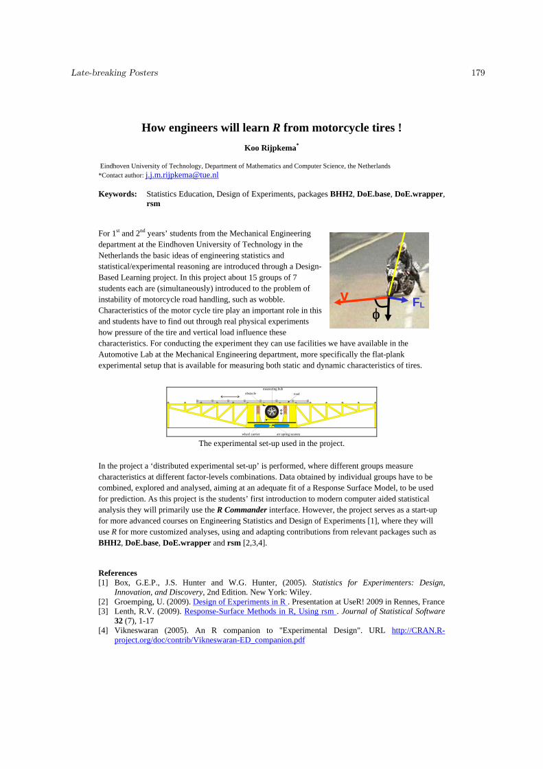
v FL

How engineers will learn R from motorcycle tires !

Koo Rijpkema*

Eindhoven University of Technology, Department of Mathematics and Computer Science, the Netherlands *Contact author: [email protected] Keywords: Statistics Education, Design of Experiments, packages BHH2, DoE.base, DoE.wrapper,

rsm

For 1st and 2nd years’ students from the Mechanical Engineering department at the Eindhoven University of Technology in the Netherlands the basic ideas of engineering statistics and statistical/experimental reasoning are introduced through a Design-Based Learning project. In this project about 15 groups of 7 students each are (simultaneously) introduced to the problem of instability of motorcycle road handling, such as wobble. Characteristics of the motor cycle tire play an important role in this and students have to find out through real physical experiments how pressure of the tire and vertical load influence these characteristics. For conducting the experiment they can use facilities we have available in the Automotive Lab at the Mechanical Engineering department, more specifically the flat-plank experimental setup that is available for measuring both static and dynamic characteristics of tires.

measuring hub

obstacle road

air spring systemwheel carrier The experimental set-up used in the project.

In the project a ‘distributed experimental set-up’ is performed, where different groups measure characteristics at different factor-levels combinations. Data obtained by individual groups have to be combined, explored and analysed, aiming at an adequate fit of a Response Surface Model, to be used for prediction. As this project is the students’ first introduction to modern computer aided statistical analysis they will primarily use the R Commander interface. However, the project serves as a start-up for more advanced courses on Engineering Statistics and Design of Experiments [1], where they will use R for more customized analyses, using and adapting contributions from relevant packages such as BHH2, DoE.base, DoE.wrapper and rsm [2,3,4].

References [1] Box, G.E.P., J.S. Hunter and W.G. Hunter, (2005). Statistics for Experimenters: Design,

Innovation, and Discovery, 2nd Edition. New York: Wiley. [2] Groemping, U. (2009). Design of Experiments in R . Presentation at UseR! 2009 in Rennes, France [3] Lenth, R.V. (2009). Response-Surface Methods in R, Using rsm . Journal of Statistical Software

32 (7), 1-17 [4] Vikneswaran (2005). An R companion to "Experimental Design". URL http://CRAN.R-

project.org/doc/contrib/Vikneswaran-ED_companion.pdf


plotKML: a framework for visualization of space-time data invirtual globes

Pierre Roudier1,? , Tomislav Hengl2, Dylan Beaudette3

1. Landcare Research, New Zealand2. ISRIC – World Soil Information, The Netherlands3. Natural Resources Conservation Service, USDA, USA?Contact author: [email protected]

Keywords: Spatial data, data visualisation

KML (formerly Keyhole Markup Language), an XML-based format, is an OGC (Open Geospatial Consor-tium) standard to represent spatial data. Use of KML has been popularized with the development of virtualglobe Google Earth (McGavra et al. 2009). Since it approval as an OGC standard, support for KML hasbeen introduced in other virtual globes and geographic information systems (Craglia et al. 2008).

KML support is already available in R through the GDAL external library, whose bindings are provided thergdal package, or directly implemented in R (packages maptools and raster). However, the support of theKML specifications is only partial. On the other hand, there is an increasing demand for tools to visuallyexplore spatio-temporal patterns in a variety of environmental data ( Andrienko & Andrienko, 2006).

The plotKML package provides the user with tools to plot spatial and spatio-temporal objects as describedby sp classes into a KML file, and proposes an easy syntax to make complete use of the KML specifications.It aims at bringing virtual globes as a full-featured plotting canvas for spatial data, and thus provide notonly methods to write various geometries in KML, but also plotting essentials, such as legend frames andmetadata subsets.

Three levels of functions are provided: (i) a general, user-friendly kml() method, (ii) a set of intermediaryfunctions to generate a KML file layer by layer, and (iii) and advanced templates for creating more advancedKML files.

(a) (b)

Figure 1: Examples of plotKML outputs. (a) Multi-layer visualisation of predictions and sampling loca-tions. (b) Soil profile plot showing changes of measured soil organic carbon with depth.

Andrienko, N., and Andrienko, G. (2006) Exploratory analysis of spatial and temporal data: a systematic approach. Springer, 703 p.

Craglia, M., Goodchild, M., Annoni, A., Camara, G., Gould, M., Kuhn, W., Mark, D., Masser, I., Maguire, D., Liang, S., and Par-sons, E. (2008). Next-Generation Digital Earth: A position paper from the Vespucci Initiative for the Advancement of GeographicInformation Science. International Journal of Spatial Data Infrastructures Research 3, 146–167.

McGavra, G., Morris, S., and Janee, G. (2009). Technology Watch Report: Preserving Geospatial Data. DPC Technology Watch

Series Report 09-01. Digital Preservation Coalition, York, UK.


1+1=3: Combining cross-sectional multiple test data to find the historic

shape of an epidemic

Gustaf Rydevik1, 2, 3*

, Mike Hutchings2, Giles Innocent

1, Glenn Marion

1, Piran White

3

1. Biomathematics and Statistics Scotland

2. Scottish Agricultural College

3. University of York


Keywords: Disease surveillance, Empirical Likelihood, EM, Bayesian Statistics, Biostatistics

We have written a set of R functions to simulate, estimate and visualize the historic incidence of pathogen infections,

given a cross-sectional sample where two or more tests with different characteristics have been taken of each subject.

We use the example of antibody and nucleic acid tests to illustrate this scenario.

In the surveillance of infectious diseases, it is often the case that resources and practical issues limit data collection to

a prevalence study at a single point in time. Previous studies have used antibody titers to calculate incidence rates for

various diseases, including Salmonella [Simonsen et al.], HIV [Heisterkamp SH et al.] and Pertussis[Hallander et al.].

However, to our knowledge, no published work has looked at combining antibody data with, for example, nucleic acid

or culture data when calculating incidence rates.

The effect of the time interval between infection and test is different for different diagnostic tests. For example,

antibodies tend to remain for a long time after infection, while tests designed to demonstrate the presence of a

pathogen such as cultures or nucleic acid tests are much more sensitive to time elapsed since infection. By exploiting

this difference, we can get an idea of whether the incidence is stable, on the increase, or decreasing, using only a

single prevalence study.

We have developed a model for this situation which combines five different components: the incidence distribution

over time, the distribution of antibodies over time after infection, the distribution of nucleic acid (or some other

indicator) over time after infection, and the observed distributions of antibodies/nucleic acid in the cross-sectional

sample.

Using a combined Bayesian/empirical likelihood approach, building on functions from the mclust package, we then

use the observed distribution of antibodies and nucleic acid together with a prior for the infection incidence, to

generate a shifted, posterior estimate of how the historical incidence behaved.

Because the results of these analyses differ depending on the specific relationship between antibodies and nucleic acid

in the studied pathogen, simulation tools built on the simecol package are used for generating data to test how our

approach works across various different antibody, nucleic acid and incidence distributions.

Acknowledgement: This work is being conducted within the FP7 WildTech Project (http://www.wildtechproject.com).

References

Simonsen, J., Mølbak, K., Falkenhorst, G., Krogfelt, K. A., & Linneberg, A. (2009). Estimation of incidences of infectious

diseases based on antibody measurements. Statistics in medicine, Volume 28, Issue 14, pages 1882–1895,

Heisterkamp SH, de Vries R, Sprenger HG, Hubben GAA, Postma MJ(2008). Estimation and prediction of the hiv- aids-

epidemic under conditions of Haart using mixtures of incubation time distributions. Statistics in Medicine 2008;

27:781–794.

Hallander, H. O., Andersson, M., Gustafsson, L., Ljungman, M. and Netterlid, E. (2009), Seroprevalence of pertussis

antitoxin (anti-PT) in Sweden before and 10 years after the introduction of a universal childhood pertussis

vaccination program. APMIS, 117: 912–922


A Package for Temporal Disaggregation of Time SeriesChristoph Sax1,2,? , Peter Steiner1,3

1. State Secretariat for Economic Affairs Seco, Switzerland2. University of Basel, Switzerland3. University of Bern, Switzerland?Contact author: [email protected]

Keywords: Econometrics, Time Series, Temporal Disaggregation, Chow-Lin

Temporal disaggregation methods are used to disaggregate and interpolate a low frequency time series intoa higher frequency series, while either the sum or the average of the resulting high-frequency series isconsistent with the low frequency series. Disaggregation can be performed with or without the help of oneor more indicator series; most indicator-based methods are variants of the method proposed by Chow andLin (1971). Currently, there is no package in R to perform these tasks. tempdisagg offers a solution for thegeneral task of temporally disaggregating a time series in R.

Use cases

Researchers in need of high frequency data can generate these data by themselves. For example, estimating aVAR (package vars) requires all variables to have the same frequency. tempdisagg allows the constructionof a missing series by the researcher. In many European countries, quarterly figures of Gross DomesticProduct (GDP) are estimated by statistical agencies using temporal disaggregation methods. Thanks totempdisagg, at the State Secretariat for Economic Affairs, we are able to estimate Switzerland’s officialquarterly GDP figures almost fully automated in R.

Implementation

tempdisagg implements the standard methods for temporal disaggregation: Denton, Chow-Lin, Fernandezand Litterman. Denton, in its most basic form, does not require additional information besides the low-frequency series, Chow-Lin, Fernandez and Litterman, on the other hand, are using one or more indicators.tempdisagg is not restricted to annual or quarterly data, it works as long as the ratio of high to low frequencyis an integer number (e.g. biannual to monthly data).

The selection of a temporal disaggregation model is similar to the selection of a linear regression model.Thus, td, the main function of tempdisagg, closely mirrors the working of the lm function (package stats),including taking advantage of the formula interface. Unlike lm, td can handle ts and mts time-seriesobjects, as a typical use-case involves these objects. Nevertheless, it also can handle vectors and matrices inthe same way as lm. td is a general function for temporally disaggregating time series and invokes particularmethods (Denton, Chow-Lin, . . . ) based on the method argument. Internally, td uses the optimizefunction (package stats) to solve the one-dimensional optimization problem, which is at the core of somevariants of the Chow-Lin procedure.

References

Chow, G. C. and A.-l. Lin (1971). Best linear unbiased interpolation, distribution, and extrapolation of timeseries by related series. The Review of Economics and Statistics 53(4), 372–375.


cloudnumbers.com - Your Calculation Cloud for R

Markus Schmidberger1,*, Moritz von Petersdorff-Campen1, Markus Fensterer1, Erik Muttersbach1

1. Cloudnumbers.com*Contact author: [email protected]

Keywords: R, cloud computing, computer cluster, high performance computing

Cloudnumbers.com provides scientists, as well as companies, with the resources to perform high performance calculations in the cloud. We help our customers to fight epidemics, develop highly advanced drugs and manage financial risk. Our aim is to change the way research collaboration is done today by bringing together scientists and businesses from all over the world on a single platform. Cloudnumbers.com is a Berlin, Germany based international high-tech startup striving for enabling everyone to benefit from the High Performance Computing (HPC) related advantages of the cloud. We regard reducing the difficulty of accessing the pooled computational power and abolishing the need for initial infrastructure investments as the key challenges in achieving our mission.

We pursue our goals by using the innovative potential of cloud computing. Leveraging the power of several pooled computer capacities and providing these on-demand via the Internet allows for a more efficient capacity utilization and highly elevated computational power. The cloud exhibits the possibility to speed up CPU and memory intensive calculations performed with applications like the well-known open-source statistics program R (www.r-project.org). Additionally, the cloud’s characteristics predestine it for being the optimal mean for collaborative data sharing. Cooperation of project members, academics or even business networks thus is facilitated in an unprecedented way with regard to HPC calculations. User created knowledge databases as well as access to the most prominent public data resources take the collaboration and cooperation potential to yet another level and scale. All these features are integrated into the safe and efficient platform solution available on a pay-as-you-go basis at cloudnumbers.com.

Currently we focus on R (CRAN and Bioconductor packages are available). Computer clusters running with the packages multicore, snow, Rmpi or snowfall are available out of the box. At this point our main goal is to get feedback and consumer insights. That is why we will provide you with some free credit in order to allow you to test our service :

http://www.cloudnumbers.com

References

M. Schmidberger, M. Morgan, D. Eddelbuettel, H. Yu, L. Tierney, U. Mansmann; State of the Art in Parallel Computing with R; Journal of Statistical Software 2009: Vol. 31, Issue 1, Page 1-27;


A tentative implementation of R for finding the non-dominated fronts in multi-objective optimization

Ching-Shih Tsou1,* , Bo-Han Wu1, Ying-Hao Lee1, Ya-Chu Chiang1

1. Institute of Information and Decision Sciences, National Taipei College of Business, Taipei 10051, Taiwan, R.O.C. *Contact author: [email protected] Keywords: multi-objective optimization, non-dominated solutions

Most decisions involve more than one conflicting objectives. This leads to the concept of non-dominance in multi-objective optimization that is different from the optimality concept of single objective one. Non-dominance means that the improvement of some objective could only be achieved at the expense of other objectives. Practically speaking, the effort on multi-objective optimization should be made in finding the non-dominated solutions archived as the non-dominated set by considering all objectives to be equally important. However, generating the non-dominated set could be computationally expensive and is often inefficient. This paper intends to implement three algorithms, the naive and slow, continuously updated, and an efficient method proposed by Kung et al., in R for finding the non-dominated fronts. Comparisons are made in order to highlight the applicability of R for building feasible multi-objective optimizers.

References Deb, K. (2001). Multi-objective Optimization Using Evolutionary Algorithms. John Wiley & Sons, pp.33-43.

Deb, K., Agrawal, S., Pratap, A., and Meyarivan, T. (2000). A fast elitist non-dominated sorting genetic algorithm for multi-objective optimization: NSGA-II. In Proceeding of the 6th International Conference on Parallel Problem Solving from Nature, Pages 849-858.

Kung, H., Luccio, F., and Preparata, F. (1975). On finding the maxima of a set of vectors. Journal of the Association Computing Machinery 22(4), 469- 476.


A hybrid machine learning algorithm for unlabeled gene expression data classification

Gokmen Zararsiz1,*, Ahmet Ozturk1, Erdem Karabulut2, Ferhan Elmalı1

1. Department of Biostatistics and Medical Informatics, Erciyes University, Kayseri, Turkey 2. Department of Biostatistics, Hacettepe University, Ankara, Turkey *Contact author: [email protected]

Keywords: unlabeled data, clustering, classification, gene expression datasets

In gene expression data analysis, classification algorithms are widely used to classify biological samples and to predict clinical or other outcomes. But, these algorithms can not be used directly, if the data is unlabeled. Ignoring unlabeled data leads information loss and labeling them manually is a very difficult and expensive process. There are semi-supervised algorithms which were produced to label the unlabeled data. However, these algorithms are impractical in wholly unlabeled datasets. Thus, it is very significant to generate the class label for this kind of wholly unlabeled datasets and clustering algorithms can be used to obtain such labels. We proposed a hybrid machine learning algorithm for gene expression datasets to determine the best clustering with an optimum cluster number, then classify the dataset using new generated class labels. In this project, we will present the applicability and effectiveness of this algorithm by using several R packages: clValid [Brock et al., 2011], RankAggreg [Pihur et al., 2009], e1071 [Dimitriadou et al., 2011].

Acknowledgement The project described is financially supported by Research Fund of the Erciyes University (Project Number: TSY-11-3587). References

D. Meyer (2001). Support Vector Machines The Interface to libsvm in package e1071. R News Volume 1/3, 23-26.

G. Brock, V. Pihur, S. Datta, and S. Datta (2008). clValid, an R package for cluster validation. Journal

of Statistical Software, 25(4). J. Xie, C. Wang, Y. Zhang, S. Jiang (2009). Clustering Support Vector Machines for Unlabeled Data

Classification. 2009 International Conference on Test and Measurement (Hong Kong, China), pp. 34-38.

V. Pihur, S. Datta, S. Datta (2009). RankAggreg, an R package for weighted rank aggregation. BMC

Bioinformatics, 10:62
