Embed Size (px)
Citation preview

ABSTRACT
Title of Dissertation: REFLECTIVE REASONING
Waiyian Chong, Doctor of Philosophy, 2006
Dissertation directed by: Professor Donald R. Perlis
Department of Computer Science
This dissertation studies the role of reflection in intelligent autonomous sys-
tems. A reflective system is one that has an internal representation of itself as
part of the system, so that it can introspect and make controlled and deliberated
changes to itself. It is postulated that a reflective capability is essential for a sys-
tem to expect the unexpected—to adapt to situations not forseen by the designer
of the system.
Two principal goals motivated this work: to explore the power of reflection
(1) in a practical setting, and (2) as a method for approaching bounded optimal
rationality via learning. Toward the first goal, a formal model of reflective agent
is proposed, based on the Beliefs, Desires and Intentions (BDI) architecture,
but free from the logical omniscience problem. This model is reflective in the
sense that aspects of its formal description, comprised of set of logical sentences,
will form part of its belief component, and hence be available for reasoning and
manipulation. As a practical application, this model is suggested as a foundation

for the construction of conversational agents capable of meta-conversation, i.e.,
agents that can reflect on the ongoing conversation. Toward the second goal, a
new reflective form of reinforcement learning is introduced and shown to have a
number of advantages over existing methods.
The main contributions of this thesis consist of the following: In Part II,
Chapter 2, the outline of a formal model of reflection based on the BDI agent
model; in Chapter 3, preliminary design and implementation of a conversational
agent based on this model; In Part III, Chapter 4, design and implementation
of a novel benchmark problem which arguably captures all the essential and
challenging features of an uncertain, dynamic, time sensitive environment, and
setting the stage for clarification of the relationship between bounded-optimal
rationality and computational reflection under the universal environment as de-
fined by Solomonoff’s universal prior; in Chapter 5, design and implementation
of a computational-reflection inspired reinforcement learning algorithm that can
successfully handle POMDPs and non-stationary environments, and studies of
the comparative performances of RRL and some existing algorithms.

REFLECTIVE REASONING
by
Waiyian Chong
Dissertation submitted to the Faculty of the Graduate School of theUniversity of Maryland, College Park in partial fulfillment
of the requirements for the degree ofDoctor of Philosophy
2006
Advisory Committee:
Professor Donald R. Perlis, ChairProfessor Tim OatesProfessor James A. ReggiaProfessor Dana S. NauProfessor Lindley Darden

c© Copyright by
Waiyian Chong
2006

TABLE OF CONTENTS
List of Tables vi
List of Figures vii
I 1
1 Introduction 2
1.1 Overview . . . . . . . . . . . . . . . . . . . . . . . . . . . . . . . . 2
1.2 Seven Days in the Life of a Robotic Agent . . . . . . . . . . . . . 5
1.3 Reflection . . . . . . . . . . . . . . . . . . . . . . . . . . . . . . . 8
1.4 Continual Computation . . . . . . . . . . . . . . . . . . . . . . . . 9
1.5 Bootstrapping Intelligence by Continual Reflection . . . . . . . . . 11
1.6 Towards Bounded Optimal Rationality . . . . . . . . . . . . . . . 13
1.7 Goals and Organization . . . . . . . . . . . . . . . . . . . . . . . 15
1.8 Thesis Outline . . . . . . . . . . . . . . . . . . . . . . . . . . . . . 16
II 18
2 Reflective Model of Agency 19
2.1 Overview . . . . . . . . . . . . . . . . . . . . . . . . . . . . . . . . 19
ii

2.2 Premises and Goals . . . . . . . . . . . . . . . . . . . . . . . . . . 20
2.3 Notations . . . . . . . . . . . . . . . . . . . . . . . . . . . . . . . 23
2.3.1 Basic syntax . . . . . . . . . . . . . . . . . . . . . . . . . . 23
2.3.2 Quote, Quasi-quote and Anti-quote . . . . . . . . . . . . . 25
2.3.3 Terminology . . . . . . . . . . . . . . . . . . . . . . . . . . 26
2.4 Architecture . . . . . . . . . . . . . . . . . . . . . . . . . . . . . . 28
2.5 Conclusions . . . . . . . . . . . . . . . . . . . . . . . . . . . . . . 31
3 Conversational Agent for Meta Dialog 32
3.1 Overview . . . . . . . . . . . . . . . . . . . . . . . . . . . . . . . . 32
3.2 Background . . . . . . . . . . . . . . . . . . . . . . . . . . . . . . 33
3.2.1 Dialogue Analysis Survey . . . . . . . . . . . . . . . . . . 34
3.3 Instructible Agent . . . . . . . . . . . . . . . . . . . . . . . . . . . 38
3.3.1 Design Goals . . . . . . . . . . . . . . . . . . . . . . . . . 38
3.3.2 Methodology . . . . . . . . . . . . . . . . . . . . . . . . . 39
3.3.3 Case Studies in Windows Management . . . . . . . . . . . 41
3.3.4 Implementation . . . . . . . . . . . . . . . . . . . . . . . . 41
3.3.5 Example . . . . . . . . . . . . . . . . . . . . . . . . . . . . 42
3.3.6 Future Work . . . . . . . . . . . . . . . . . . . . . . . . . . 43
3.4 Related Work . . . . . . . . . . . . . . . . . . . . . . . . . . . . . 45
3.4.1 SHRDLU . . . . . . . . . . . . . . . . . . . . . . . . . . . 45
III 48
4 Reinforcement Learning and Bounded Optimality 49
4.1 Overview . . . . . . . . . . . . . . . . . . . . . . . . . . . . . . . . 49
iii

4.2 Toroidal Grid World . . . . . . . . . . . . . . . . . . . . . . . . . 50
4.3 Markov Decision Process . . . . . . . . . . . . . . . . . . . . . . . 51
4.4 Knowledge Acquisition Modes . . . . . . . . . . . . . . . . . . . . 52
4.5 Reinforcement Learning . . . . . . . . . . . . . . . . . . . . . . . 53
4.6 Incomplete Information . . . . . . . . . . . . . . . . . . . . . . . . 56
4.7 Partially Observable Markov Decisions Processes . . . . . . . . . . 57
4.8 Bounded Optimal Rationality . . . . . . . . . . . . . . . . . . . . 59
4.9 Non-stationary Environment . . . . . . . . . . . . . . . . . . . . . 61
4.10 Intelligence in General . . . . . . . . . . . . . . . . . . . . . . . . 61
4.11 Discussion . . . . . . . . . . . . . . . . . . . . . . . . . . . . . . . 64
4.12 Conclusions . . . . . . . . . . . . . . . . . . . . . . . . . . . . . . 64
5 Reflective Reinforcement Learning 66
5.1 Overview . . . . . . . . . . . . . . . . . . . . . . . . . . . . . . . . 66
5.2 Problem Setting . . . . . . . . . . . . . . . . . . . . . . . . . . . . 68
5.3 Reflective Reinforcement . . . . . . . . . . . . . . . . . . . . . . . 68
5.3.1 Algorithm . . . . . . . . . . . . . . . . . . . . . . . . . . . 69
5.3.2 Remarks . . . . . . . . . . . . . . . . . . . . . . . . . . . . 70
5.4 Implementation . . . . . . . . . . . . . . . . . . . . . . . . . . . . 72
5.4.1 Protocol . . . . . . . . . . . . . . . . . . . . . . . . . . . . 72
5.5 Toroidal Grid World . . . . . . . . . . . . . . . . . . . . . . . . . 73
5.5.1 “Physics” of the World . . . . . . . . . . . . . . . . . . . . 73
5.5.2 Experiment Settings . . . . . . . . . . . . . . . . . . . . . 75
5.5.3 Deterministic Stationary Environment (k0) . . . . . . . . . 78
5.5.4 Non-deterministic Stationary Environment (k1) . . . . . . 79
5.5.5 Non-stationary Environment (k2) . . . . . . . . . . . . . . 89
iv

5.6 Other Experiments . . . . . . . . . . . . . . . . . . . . . . . . . . 93
5.6.1 John Muir Trail . . . . . . . . . . . . . . . . . . . . . . . . 93
5.6.2 Partially Observable Pole Balancing . . . . . . . . . . . . . 93
5.7 Summary . . . . . . . . . . . . . . . . . . . . . . . . . . . . . . . 95
5.8 Related Work . . . . . . . . . . . . . . . . . . . . . . . . . . . . . 96
5.9 Conclusions and Further Work . . . . . . . . . . . . . . . . . . . . 97
IV 99
6 Conclusions 100
6.1 Overview . . . . . . . . . . . . . . . . . . . . . . . . . . . . . . . . 100
6.2 To the Future . . . . . . . . . . . . . . . . . . . . . . . . . . . . . 101
v
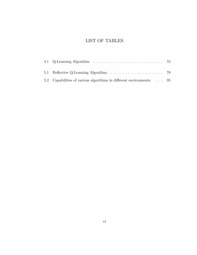
LIST OF TABLES
4.1 Q-Learning Algorithm . . . . . . . . . . . . . . . . . . . . . . . . 55
5.1 Reflective Q-Learning Algorithm . . . . . . . . . . . . . . . . . . . 70
5.2 Capabilities of various algorithms in different environments. . . . 95
vi

LIST OF FIGURES
4.1 A 12× 12 toroidal grid world, where there are two kinds of points,
either white or black; the double circle indicates the location of
the agent. . . . . . . . . . . . . . . . . . . . . . . . . . . . . . . . 50
4.2 A 12×12 toroidal grid world, where the black points are distributed
on the diagonal line. . . . . . . . . . . . . . . . . . . . . . . . . . 53
4.3 A 12× 12 toroidal grid world, where the world is not fully observ-
able by the agent: the perception of the agent is limited to its own
location and the four immediate neighbors (indicated in the figure
by points bounded by the box around the agent). The black points
are distributed according to the equations y = x, y mod 3 = 0,
where x, y ∈ Z. . . . . . . . . . . . . . . . . . . . . . . . . . . . . 57
4.4 A 12×12 toroidal grid world, where the black dots are distributed
indeterministically with probability 0.2 on the line specified by the
equations y = x, where x, y ∈ Z. . . . . . . . . . . . . . . . . . . . 59
4.5 A non-stationary toroidal grid world, where the positions of black
points move up a step for each time step. The two figures depict
snapshots of the world when t = 0 and t = 1, respectively. The
black points are distributed according to the equations (y−2x− t)
mod 12 = 0, where x, y, t ∈ Z, and t is the time step number. . . . 62
vii

5.1 Simplified k0 (interval of 2). . . . . . . . . . . . . . . . . . . . . . 77
5.2 Q-Learning in toroidal-grid-world with r = 10. In this (and subse-
quent) figure(s), the x-axis is the number of steps taken, and the
y-axis is the performance. The solid line shows the performance
average over a running window of the last 216 time steps, while the
dash-line is the life-time average. . . . . . . . . . . . . . . . . . . 80
5.3 RQL in toroidal-grid-world with r = 10. . . . . . . . . . . . . . . 80
5.4 Q-Learning in toroidal-grid-world with r = 3. . . . . . . . . . . . 81
5.5 RQL in toroidal-grid-world with r = 3, using 5 internal states. . . 81
5.6 Performance of RQL on an indeterministic toroidal grid world. . . 82
5.7 Static, nondeterministic, 48× 48 toroidal grid world. . . . . . . . 86
5.8 Static, nondeterministic, 240× 240 toroidal grid world. . . . . . . 87
5.9 Static, nondeterministic, 720× 720 toroidal grid world. . . . . . . 88
5.10 Performance of RQL on a non-stationary toroidal grid world. . . . 89
5.11 Dynamic 48× 48 toroidal grid world. . . . . . . . . . . . . . . . . 90
5.12 Dynamic 240× 240 toroidal grid world. . . . . . . . . . . . . . . . 91
5.13 Dynamic 720× 720 toroidal grid world. . . . . . . . . . . . . . . . 92
5.14 Performance of RQL on John Muir Trail. . . . . . . . . . . . . . . 93
5.15 Partially observable pole balancing. The x-axis represents the
number of trials (or episodes), and the y-axis the number of control
steps attained before failures. The pluses denote maximum values
of 200 trials, while the solid line is the average. . . . . . . . . . . . 95
viii

Part I
1
Chapter 1
Introduction
1.1 Overview
A unifying theme of AI research is the design of an architecture for allowing an
intelligent agent to operate in a common sense informatic situation [McCarthy,
1989], where the agent’s perception (hence its knowledge about the world) is
incomplete, uncertain and subject to change; and the effects of its actions are
indeterministic and unreliable. There are many reasons (e.g., scientific, philo-
sophical, practical) to study intelligent agent architecture; for our purposes, we
will define our goal as to improve the performance of the agent, where perfor-
mance is in turn defined as resources (time, energy, etc) spent in completing given
tasks. We are interested in the question “What is the best strategy to build an
agent which can perform competently in a common sense informatic situation?”
It is clear that it will be impractical for the designer of the agent to anticipate
everything it may encounter in such a situation; hence, it is essential that some
routes of self-improvement be provided for the agent if it is to attain a reasonable
level of autonomy. What should we provide to the architecture to open these
routes?
2

For an agent to function competently in commonsense world, we can ex-
pect the underlying architecture to be highly complex. Careful attention will
be needed for the design process, as well as the designed artifact, to ensure suc-
cess. We identify the following requirements: (i) In addition to fine-tuning of
specialized modules the agent might have, more fundamental aspects of the ar-
chitecture should be open to self-improvement. For example, an agent designed
to interact with people may have a face recognition module; a learning algorithm
to improve its face recognition accuracy is of course desirable, but it is not likely
to be helpful for the agent to cope with unexpected changes in the world—for
that, the agent may need to reorganize its modules, revise or even completely
replace its decision procedure, etc. (ii) Improvements need to be made reason-
ably efficiently. It’s said that a roomful of monkeys typing away diligently at
their keyboards will eventually produce the complete works of Shakespeare; in
the same vein, we can imagine a genetic algorithm, given enough time and input,
can evolve a sentient being, but the time it takes will likely be too long for us
to withstand. (iii) Somewhat related to the previous two points, it is important
to stress that the improvements made be transparent to us so that we can incre-
mentally provide more detailed knowledge and guidance when necessary to speed
up the improvements.
To build an intelligent agent, lessons learned by builders of other sophisticated
systems might be instructive: in particular, the technique of bootstrapping is of
relevance. The bootstrapping technique has been widely employed in the process
of building highly complex systems, such as microprocessors, language compilers,
and computer operating systems. It could play an even more prominent role
in the creation of computation systems capable of supporting intelligent agent
3

behaviors, because of the even higher level of complexity. Typically in a boot-
strapping process, a lower-level infrastructural system is first built “by hand”;
the complete system is then built, within the system itself, utilizing the more
powerful constructs provided by the infrastructure. Hence, it provides benefits
in the ways of saving effort as well as managing complexity.
Ideally, as designers of the agent, we’d like to push as much work as possible
to be automated and carried out by computer. There is no doubt that the study
of specialized algorithms has been making great contributions to the realization
of intelligent agency; however, we think that the study of bootstrapping behavior
may be a more economical way to achieve that goal. Instead of designing the
specialized modules ourselves, we should instead look for way to provide the
infrastructure on which agents can discover and devise the modules themselves.
A few questions need to be addressed before we can apply a bootstrapping
approach: What constructs are needed in the infrastructure to support the boot-
strapping of intelligence? How should they be combined? How should they
operate? More generally, if we leave alone a robot agent in a reasonably rich
environment for a long period of time, what will enable the robot to evolve it-
self into a more competitive agent? How do we provide a path for the agent to
improve itself? We think an example will help us to answer the questions! In
the next section, we will tell the story of a office robot to show the importance
and desirability of self-improving capability in an artificial agent. In light of the
typical problems that a robot may encounter in the real world, the following two
sections (Sec 1.3 and Sec 1.4) present a more detailed account of two key ideas:
reflection and continual computation, which we think are essential to the success
of the robot, and argue that the uniformity and expressiveness of a logic-based
4

system can facilitate the implementation of complex agency.
1.2 Seven Days in the Life of a Robotic Agent
Let us consider an imaginary “office robot”, who roams the Computer Science
office building delivering documents, coffee, etc. and was endowed at birth with
the desire to make people happy. We will see how it developed into an effective
robot through its first week of work.
1st day: The robot was first given a tour of the building. Among other things,
it was shown the power outlets scattered around the building so that it could
recharge itself.
2nd day: The morning went well: the robot delivered everything on target.
But during the afternoon it ran into a problem: it found itself unable to move!
The problem was soon diagnosed — it was simply a case of low battery. (Since
thinking draws less energy than moving, the robot could still think.) It turned
out that although it knew it needed power to operate and it could recharge itself
to restore its battery, it had never occurred to the robot that, it would need to
reach an outlet before the power went too low for it to move! 1 The movement
failure triggered the robot to derive the above conclusion, but it was too late;
the robot was stuck, and could not deliver coffee on request. Caffeine deprived
computer scientists are not happy human beings; the robot had a bad day.
3rd day: The robot was bailed out of the predicament by its supervisor in the
morning. Having learned its lesson, it decided to find an outlet a few minutes
before the battery got too low. Unfortunately, optimal route planning for robot
1Counter to traditional supposition that all derivable formulas are already present in the
system.
5

navigation is an NP-complete problem. When the robot finally found an optimal
path to the nearest power outlet, its battery level was well below what it needed
to move, and it was stuck again. Since there was nothing else it could do, the
robot decided to surf the web (through the wireless network!), and came upon an
interesting article titled “Deadline-Coupled Real-time Planning” [Nirkhe et al.,
1997].
4th day: After reading the paper, the robot understood that planning takes time,
and that it couldn’t afford to find an optimal plan when its action is time critical.
The robot decided to quickly pick the outlet in sight when its battery was low.
Unfortunately, the outlet happened to be too far away, and the robot ran out of
power again before reaching it. In fact, there was a closer outlet just around the
corner; but since a non-optimal algorithm was used, the robot missed it. Again,
stuck with nothing else to do, the robot kicked into the “meditation” mode where
it called the Automated Discovery (AD) module to draw new conclusions based
on the facts it accumulated these few days. The robot made some interesting
discoveries: upon inspecting the history of its observations and reasonings, the
robot found that there were only a few places it frequented; it could actually
precompute the optimal routes from those places to the nearest outlets. The
robot spent all night computing those routes.
5th day: This morning, The robot AD module derived an interesting theorem:
“if the battery power level is above 97% of capacity when the robot starts (and
nothing bad happened along the way), it can reach an outlet before the power
is exhausted.” It didn’t get stuck that day. But people found the robot to be
not very responsive. Later, it was found that the robot spent most of its time
around the outlets recharging itself — since the robot’s power level dropped 3%
6

for every 10 minutes, the theorem above led it to conclude that it needed to go
to the outlet every 10 minutes.
6th day: After the robot’s routine introspection before work, it was revealed that
the knowledge base was populated with millions of theorems similar to the one it
found the day before, but with the power level at 11%, 12%, ..., and so on. In fact,
the theorem is true when the power level is above 10% of capacity. Luckily, there
was a meta-rule in the robot’s knowledge base saying that “a theorem subsumed
by another is less interesting.” Thus all the theorems with parameter above 10%
were discarded. Equipped with this newer, more accurate information, the robot
concluded that it could get away with recharging itself every 5 hours.
7th day: That happened to be Sunday. Nobody was coming to the office. The
robot spent its day contemplating the meaning of life.
Analyzing the behavior of the robot, we can see a few mechanisms at play:
in addition to the basic deductive reasoning, goal directed behavior, etc., the
robot also demonstrates capabilities such as abductive reasoning (diagnoses of
failures), explanation-based learning (compilation of navigation rules, derivation
of recharging rules), reflection (examining and reasoning about its power reading,
revision of recharging rule), and time-sensitivity (understanding that delibera-
tions take time, people don’t like waiting, etc). Of course, none of these is new
in itself; however, the interactions among them has enabled the robot to demon-
strate remarkable flexibility and adaptivity in a ill-anticipated (by the designer
of the robot) and changing world. Below, we will elaborate on the reflective
capability and the continual aspect of the agent’s operations.
7

1.3 Reflection
As noted earlier, a computational system is said to be reflective when it is itself
part of its own domain (and in a causally connected way). More precisely, this
implies that (i) the system has an internal representation of itself, and (ii) the
system can engage in both “normal” computation about the external domain and
“reflective” computation about itself [Maes, 1988]. Hence, reflection can provide
a principled mechanism for the system to modify itself in a profound way.
We suggest that a useful strategy for a self-improving system is to use re-
flection in the service of self-training. Just as a human agent might deliberately
practice a useful task, increasing her efficiency until (as we say) it can be done
“unconsciously” or “automatically”, without explicit reasoning, we think that
once a reflective system identifies an algorithm or other method for solving a
frequently encountered problem, it should be able to create procedural modules
to implement the chosen strategy, so as to be able in the future to accomplish its
task(s) more efficiently, without fully engaging its (slow and expensive) common-
sense reasoning abilities.
Although reflection sounds attractive, it has largely been ignored by re-
searchers of agent architecture, mainly because of the high computation com-
plexity that can be involved in doing reflective reasoning [Anderson and Perlis,
2005]. However, we think the solution to the problem is not by avoiding reflection,
but looking at the larger picture and considering the environment and extent in
which an agent operates, and finding way to reap the benefits of reflection with-
out being bogged down by its cost. We think the notion of continual computation
is a promising venue for reflection to become useful.
8

1.4 Continual Computation
Any newcomer to the field of Artificial Intelligence (AI) will soon find out that,
almost without exception, all “interesting” problems are NP-hard. When a com-
puter scientist is confronted with a hard problem, there are several options to
deal with it. For example, one can simplify the problem by assuming it occurs
only under certain conditions (which are not always realistic) and hoping bad
cases don’t happen frequently. One can also identify a simpler subproblem so
that it can be solved algorithmically and automated, and leave the hard part for
the human. Another option is for the scientist to study the problem carefully,
derive some heuristics, and hope that they will be adequate most of the time.
But none of these is quite satisfying: ideally, we would like the computer to do as
much work for us as possible, and hopefully, be able to derive the heuristics by
itself. A promising approach toward realizing this ideal is the notion of continual
computation [Horvitz, 1997].
The main motivation behind continual computation is to exploit the idle
time of a computation system. As exemplified by usage patterns of desktop
computers, workstations, web-servers, etc. of today, most computer systems are
under utilized: in typical use of these systems, relatively long spans of inactivity
are interrupted with bursts of computationally intensive tasks, where the systems
are taxed to their limits. How can we make use of idle time to help improve
performance during critical time?
Continual computation generalizes the definition of a problem to encompass
the uncertain stream of challenges faced over time. One way to analyze this prob-
lem is to put it into the framework of probability and utility, or more generally,
rational decision making:
9

Policies for guiding the precomputation and caching of complete
or partial solutions of potential future problems are targeted at en-
hancing the expected value of future behavior. The policies can be
harnessed to allocate periods of time traditionally viewed as idle time
between problems, as well as to consider the value of redirecting re-
sources that might typically be allocated to solving a definite, current
problem to the precomputation of responses to potential future chal-
lenges under uncertainty[Horvitz, 2001].
An implicit assumption of the utility-based work in continual computation is that
the future is somehow predictable. But in many cases, this cannot be expected.
For example, for long term planning, most statistics will probably lose their
significance. Here is a place where logic-based systems with the capability to
derive or discover theorems on its own (e.g., Lenat’s AM system [Lenat, 1982])
can play a complementary role, similar to the way that mathematics plays a
complementary role to engineering. Just as mathematicians usually do not rely
on immediate reward to guide their research (yet discover theorems of utmost
utility), AM can function in a way independent of the immediate utility of its
work.
More precisely, if we adopt logic as our base for computation and look at
problem solving as theorem proving [Bibel, 1997], a system capable of discovering
new theorems can become a very attractive model of a continual computation
system. In such a system, every newly discovered theorem has the potential of
simplifying the proof of a future theorem; so in essence, theorems become our
universal format for caching the results of precomputation and partial solutions
to problems.
10

A simplistic embodiment of the model can just be a forward chaining system
capable of combining facts in its database to produce new theorems using modus
ponens, for instance. Such a system is not likely to be very useful, however,
because it will spend most of its time deriving uninteresting theorems. So the
success of this model of continual computation will hinge on whether we can
find meaningful criteria for the “interestingness” of a theorem. In the classical
AM [Lenat, 1982, 1983, Lenat and Brown, 1984], the system relies largely on
human judgment to determine interestingness. In a survey of several automated
discovery programs, Colton and Bundy [Colton and Bundy, 1999] identify several
properties of concepts which seem to be relevant to their interestingness, such as
novelty, surprisingness, understandability, existence of models and possibly true
conjectures about them. Although these properties seem plausible, it is not
obvious they are precise enough to be operational to guide automated discovery
programs toward significant results.
1.5 Bootstrapping Intelligence by Continual Reflection
Hence, on the one hand, we have these intervals of idleness in a long-running agent
process we don’t quite know how to make use of; on the other hand, we have this
notion of reflective computation which promises radical adaptivity, but has been
hampered by the excessive computation resource requirement. We think it would
be intriguing to combine the two concepts and arrive at an agent architecture
which will continually reflect on its own working and find ways to improve itself
when it is idle, or has nothing better to do.
It probably would not be too challenging a task to design a robot capable
of displaying the self-improving behaviors described above using conventional
11

machine learning methods, provided that the needs for, or directions of, improve-
ments are known at design time. But for truly complex and dynamic environ-
ments, it is seldom possible, nor desirable, to anticipate every need and exception
situation. The complexity of an agent which can perform well in such environ-
ment will be so high that most probably it will exceed the comprehension of
human mind; it will be an impossible task to devise and keep track of each detail
“manually”. To keep this complexity under control, it is critical that we muster
as much help as we can get from the computer, or the agent itself. Thus, we
think the right way to go in agent design is to identify a core infrastructure with
enough foundation mechanisms for seeding a self-bootstrapping process, so that
we can just say, “improve yourself”, and the agent will be able to “derive” a
method of improvement (which might well be one of the known machine learning
paradigms) for any deficiency it detects. We believe only an agent capable of
continual reflection will be able to make the radical adaptations needed for it to
address any unexpected shortcoming of its (original) design, and thus attain true
intelligence.
The so called No Free Lunch Theorem [Wolpert and Macready, 1997] states
that “all algorithms that search for an extremum of a cost function perform
exactly the same, when averaged over all possible cost functions.” In other words,
without domain specific structural assumptions of the problem, no algorithm can
be expected to perform better on average than simple blind search. This result
appears to be a cause for pessimism for researchers hoping to devise domain-
independent methods to improve problem solving performance. But on the other
hand, this theorem also provides a compelling reason for embracing the notion of
continual computation, which can be seen as a way to exploit domain dependent
12

information in a domain independent way.
1.6 Towards Bounded Optimal Rationality
The secret of survival is: Always expect the unexpected.
— Dr. Who
Is it possible to ask an agent, “improve thyself”, without giving it any further
direction on what to improve, what function to optimize, or any specific evalu-
ation function? In other words, can we design an agent that can adapt to new
environments and situations, not anticipated by us, the designers? A key to such
an agent is the identification of a general, abstract performance metric. Some
think “being rational” is such a metric.
An agent is rational if its behavior is consistent with its goal; more precisely,
the actions it takes maximize the probability of its goal being achieved. However,
the notion of rationality doesn’t directly provide guidance to implementation of
a rational agent, since it is computationally unrealizable: finding the best action
is usually very expensive, and in most circumstances, when the agent finally (if
at all) computes the “best” action, the environment will have changed so much
that the action becomes suboptimal.
The notion of bounded optimal rationality overcomes this problem by taking
the finiteness of computational resources (time, memory spaces, etc) into account.
Russell [Russell and Subramanian, 1995] provides the following definition:
Define f = Agent(l, M) to be an agent function implemented by the
program l running on machine M . Then the bounded optimal pro-
13

gram lopt is defined by
lopt = argmaxl∈LMV (Agent(l, M),E, U)
where LM is the finite set of all programs that can be run on M ;
E is the environment in which the agent is to operate, and U is the
performance measure which evaluates the sequence of states through
which the agent drives the actual environment; V (f,E, U) denotes
the expected value according to U obtained by agent function f in
environment class E, which is assumed to be a probability distribution
over elements of E.
As we can see, the bounded optimal agent is dependent on the machine,
the environment and the utility function. This is perhaps not surprising, since
intuitively, an agent specially trained to a specific environment will perform better
than others.
Consider the function
g(M, E, U) = argmaxl∈LMV (Agent(l, M),E, U)
This function, when given specifications of a machine, an environment and a
utility function, produces a program for the machine that is bounded optimal in
the environment. It is obvious this function will be very expensive to compute:
actually, the function can be considered the holy-grail of Artificial Intelligence,
or the ultimate programmer. An agent with access to this function will be able
to adapt to every environment — provided the adaptation can be made in time.
Our hypothesis is, the equivalence of telling an agent to improve itself will be
the encoding of some relaxation of this function into the belief-base of the agent.
14

The agent model developed in Chapter 2 was partly motivated by attempt at
this.
1.7 Goals and Organization
Two principal goals motivated this work when it was initiated several years ago: I
had the hope that a single reflection model of agency could be designed to serve as
foundation for (1) practical applications, e.g., in modeling a conversational agent,
and (2) theoretical investigation of methods to approximate bounded optimal
rationality [Russell, 1997].
In particular, I began this research in the hopes of proving a general conver-
gence theorem, along the lines of the convergence theorem for Q-learning, but for
a more ambitious Russellian-style bounded optimal rationality. The idea was to
show that an iterative process of fairly blind (ie, not based on a model of belief
and inference) bootstrapped self-improvement could, in the limit achieve a kind
of maximum possible degree of performance.
However, this theoretical attempt proved elusive, and so for a time I turned
to a more BDI-oriented approach, namely that of an intelligent agent reasoning
its way to improved behavior. This approach is outlined in Part II (Chapter 2
and 3).
Indeed, such an approach does seem to have some definite power, as evidenced
in related work [Joysula, 2005]; but it is difficult to assess the generality of that
approach with respect to the limits of learning, since it has a strong empirical
and domain-specific character.
Thus as a compromise between these two directions, I focussed most of my ef-
forts on an empirically-informed treatment of a very general (non-domain-specific,
15

model-free and non-BDI) incremental learning policy; instead of proving a con-
vergence theorem, I performed many experiments in order to better assess such
possible convergence. These methods and results are reported in Part III (Chap-
ter 4 and 5).
1.8 Thesis Outline
In this chapter2, we described a series of improvements a hypothetical office
robot had undergone, and speculated on possible mechanisms which can explain
these self-improving behaviors. We think these behaviors can serve as a useful
benchmark for agent architecture designers: can a proposed agent design display
these behaviors? What will be needed for an agent to do so? We also argued that
effective exploitation of two key concepts — reflective and continual computation
— will be essential to achieving these behaviors.
In Chapter 2, a reflective model of agency is presented as a foundation to a
theory that can explain, predict, and subsequently, be applied to generate the
behaviors depicted in the seven-days scenario in Section 1.2. The model, based
on the BDI architecture [Bratman, 1987] and formalized in a first order language
augmented with the meta-theoretic device of quotation, is constructed in such a
way that the theory describing it is also a component (as the belief subsystem) of
the agent embodying this model. We think this construction is essential for the
agent to acquire the abilities for introspection, self-evaluation, and ultimately,
self-improvement.
In Chapter 3, the model developed in Chapter 2 is applied to the domain of
natural language conversation. The model is extended with linguistic concepts
2Parts of this chapter appear in Chong et al. [2003].
16

such as communication acts to explain how a conversational agent can inspect
the ongoing conversation it is participating in, and engage in meta-conversation
when needed to correct misunderstanding and establish common ground. We
argue that for any conversational agent purporting to display any understanding
of the conversation it is engaging in, it will need to be an expert “specialized” in
the domain of linguistics, in addition to the domain that it is originally designed to
handle. We have a preliminary implementation illustrating how new terminology
can be acquired by the agent through conversation.
In Chapter 4, we introduce a series of increasingly general models of envi-
ronment where fewer and fewer assumptions are made, from Markov decision
processes (MDPs), partially observable Markov decision processes (POMDPs),
to non-stationary environments where it is no longer assumed that the environ-
ments are generated by fixed finite state machines, and the universal environment,
where no physical law is assumed. We discuss possible performance measures and
algorithms for solving them. We put forward a few conjectures about general in-
telligence.
In Chapter 5, we propose an algorithm (RQL) for a prototypical agent in uni-
versal environment, report on various empirical studies using RQL, and provide
comparisons with other approaches.
Finally, In Chapter 6, we offer some brief remarks on where this may lead.
17

Part II
18

Chapter 2
Reflective Model of Agency
2.1 Overview
There are two aspects to a theory of intelligent agency: from within, it can be a
prescriptive model of an agent serving as a blueprint for actual implementation
of the agent, engendering its behaviors; from without, it can be a descriptive
model of an agent for understanding, explaining, and predicting the behaviors
of other agents. Respective works have been done for the former (e.g., [Myers,
1997]) as well as the latter (e.g.,[Bratman et al., 1988, Rao and Georgeff, 1991]).
However, there is no reason we cannot develop a theory which can serve both
purposes. Actually, it is highly desirable, or even imperative, that this unified
theory be developed when the agent has to deal with other intelligent agents in
its environment — such as a conversational agent.
Below we propose a reflective model of agency, RMA, that views agents not
only as attempting to make sense of inanimate elements in their environment,
but also striving to understand themselves and other “cognitive” agents that
can be as complicated as themselves. RMA is based on the BDI architecture
[Bratman, 1987], which recognizes the primacy of the mental attitudes of belief,
19

desire and intention. Underlying this BDI model is a formal language L, a first
order language augmented with a quotation mechanism. The language L, in
addition to being language used to formalize our model of agency, is also the
language of knowledge representation for agents based on this model of agency.
The formal description of agents developed here will also become part of beliefs of
these agents, allowing them to reason about behaviors of other agents. Moreover,
since an agent embodying this theory of agency has the theory at its disposal,
open-ended introspection and enhancements to itself become possible, making
the agent “reflective”.
2.2 Premises and Goals
Background
Daniel Dennett [Dennett, 1987] coined the term intentional system to describe
entities “whose behaviour can be predicted by the method of attributing belief,
desires, and rational acumen”. Dennett identifies different ‘grades’ of intentional
system:
A first order intentional system has beliefs and desires (etc.) but
no beliefs and desires about beliefs and desires. [...] A second order
intentional system is more sophisticated; it has beliefs and desires
(and no doubt other intentional states) about beliefs and desires (and
other intentional states) — both those of others and its own.
Doyle [Doyle, 1983] was perhaps the first to proposed the design of rational
agents as the core of AI. Horvitz et al. [Horvitz et al., 1988] proposed the max-
imization of utility, in the sense established in [von Neumann and Morgenstern,
20

1944], as the interpretation of rationality.
Truth and Utility
According to this tradition, the ultimate criterion of success of an agent is its
performance, i.e., whether it is effective in achieving its goals. Most of the time,
agents that know the truth will outperform agents that do not, since they will
be able to predict the world more accurately and choose actions that are more
effective in affecting the world towards more desirable direction. However, ob-
session with truth could sometimes be detrimental to the effectiveness of agents.
For example, knowing the truth value of the liar sentence (e.g., “this sentence
is false”) may not be consequential to the agent, while insisting on pursuing it
might very well interfere with the immediate performance of the agents; hence
perhaps the pursuit of such truth can be deferred (until, for example, the agent
needs to take a philosophy exam).
As a consequence of this premise, we question the assumption that the value
of consistency always outweights the cost of maintaining it. In other words,
we believe it should be permissible for the agent to believe in falsehood, and
contradictive information to exist in agent’s beliefs when the cost incurred by the
maintainence of consistency is too high. An agent should be allowed to make the
tradeoff between expediency and consistency.
In particular, we are more liberal in adopting notions which might seem du-
bious to logicists. For example, our conceptualization will make extensive use of
reificiation — basically, we think everything that can be named (or described) can
be treated as an object in the world. Although reification simplifies the treatment
of mental attitudes such as beliefs, desire and intentions, it is typically shunned
21

because it can lead to the construction of the liar sentence, which nobody quite
knows how to deal with [Montague, 1963, Thomason, 1980]. However, since it
is, in most circumstances, inconsequential to the effectiveness of the agent in real
world, a utility based agent would not be paralyzed by it.
Ontological Assumptions
We assume the world can be understood as being comprised of entities and
relationships among entities. Unary relationships are usually called the properties
of entities. The set of all entities in the world we are modeling is called the
universe of discourse, or simply the universe. The universe can contain concrete
objects such as books, tables, people, etc, as well as abstract objects such as
numbers, sets, relationships, and things that designate the above entities, such
as names, pronouns, etc. In particular, we assume linguistic constructs of the
formal language we use to describe the world, L, such as sentences, variables,
constants, functions, terms, etc, can also be “reified” and become part of the
universe. Basically, we assume everything that can be names are objects in the
universe.
We subscribe to Smith’s knowledge representation hypothesis [Smith, 1982]:
Any mechanically embodied intelligent process will be comprised
of structural ingredients that (a) we as external observers naturally
take to represent a propositional account of the knowledge that the
overall process exhibits, and (b) independent of such external seman-
tical attribution, play a formal but causal and essential role in engen-
dering the behavior that manifests that knowledge.
as well as his reflection hypothesis [Smith, 1982]:
22

In as much as a computational process can be constructed to rea-
son about an external world in virtue of comprising an ingredient pro-
cess (interpreter) formally manipulating representations of that world,
so too a computational process could be made to reason about itself
in virtue of comprising an ingredient process (interpreter) formally
manipulating representations of its own operations and structures.
2.3 Notations
The language L used to formalize RMA is an instance of the first order predi-
cate calculus with equality, augmented with a quotation mechanism that will be
explained below.
2.3.1 Basic syntax
The language L is defined over a set of symbols, the alphabet. The alphabet is
divided into two disjoint subsets: logical symbols and non-logical symbols.
The set of logical symbols is a finite set
ΣlL = {=,¬,∨, ∀}
However, we use an extended set of logical symbols to allow shorter expression,
ΣelL = {=,¬,∨, ∀, ∃,∧,⇒,⇐,⇔}
It can be easily established that anything which can be expressed using the ex-
tended set can be rewritten into formula using the original set only.
The set of nonlogical symbols consists of two subclasses: constant symbols
and variable symbols. We will adopt the convention of using words starting with
23

capital letters to denote constant symbols (e.g, Alice, Square, Member), and
lowercase words to denote variable symbols (e.g., x, y, z, v0, v1, ...).
The syntax of L can be described using the following BNF rules:
<wff> := (∀[<variable>+] <wff>)
| (∨ <wff>*)
| <literal>
| (∃[<variable>+] <wff>)
| (∧ <wff>*)
| (⇔ <wff>*)
| (⇒ <wff>*)
| (⇐ <wff>*)
<literal> := <atom>
| (¬ <atom>)
<atom> := (<relconst> <term>*)
| (= <term>+)
<term> := <constant>
| <variable>
| <funexpr>
<funexpr> := (<funconst> <term>*)
With these established, we have enough to bootstrap a more formal defini-
tion of L, which is the set of all databases according to the following definitions
(adopted from [Genesereth and Nilsson, 1988]):
∀[x] (⇔ (Constant x)
(∨ (Objconst x) (Funconst x) (Relconst x)))
∀[x] (⇔ (Term x)
(∨ (Objconst x) (Variable x) (Funexpr x)))
∀[x l](⇔ (Termlist x)
(∀[x] (⇒ (Member x l) (Term x))))
∀[f l](⇔ (Funexpr (Concat f l))
(∧ (Funconst f) (Termlist l)))
∀[r l](⇔ (Atom (Concat r l))
(∧ (Relconst r) (Termlist l)))
∀[x] (⇔ (Literal x)
(∨ (Atom x)
(∃[z] (∧ (Atom z)
(= x (quote (¬ z)))))))
∀[c] (⇔ (Clause c)
(∀[x] (⇒ (Member x c) (Literal x))))
∀[d] (⇔ (Database d)
(∀[x] (⇒ (Member x d) (Clause x))))
24

2.3.2 Quote, Quasi-quote and Anti-quote
When discussing things that can refer to other things, care must be taken about
the use and mention distinction. For example, we use the name “Alice” to refer
to Alice, a person, in most usual circumstances. But sometimes we need to
refer to the name itself, rather than to Alice the person — for instance, the first
mention of “Alice” in the previous sentence. The usual convention in natural
language (such as English) is to use a quotation device to stop the “evaluation”
of a referring expression at itself, rather than to the referred object.
As the formal language L will be used to express facts about formal linguis-
tic constructs such as constants, variables and other terms which refer to other
objects in the world, it needs a similar quotation mechanism. For example, the
expression
(Pretty Alice)
states the fact that Alice the person is pretty, and
(Has-five-letters ’Alice)
states the fact that “Alice” the name has five letters.
We assume the existence of a function1,
Quote : ΣL∗ 7→ Objconst
which maps arbitrary expressions of L to unique names of the expressions. These
names are also objects in our universe of discourse, which have representations as
object constants in L. We can then see the expression ’Alice as an abbreviation
for (Quote Alice).
1Mathematically inclined people can think of it as Godel’s numbering, which he showed how
to effectively compute in the proof of the incompleteness theorem.
25

Quote also provides a way to represent facts which involve some other facts,
such as the mental attitudes of belief, knowledge, etc in first order language. We
can represent the fact that Alice believes that Bob is happy, using the following
expression in L:
(Belief Alice ’(Happy Bob))
Since ’(Happy Bob) (instead of (Happy Bob), which is a sentence) is just an
ordinary term in L, the above is a perfectly legal first order sentence.
Note that Quote is a meta-theoretic function2 w.r.t L. In our usage so far, it
can be seen simply as a convention for writing constant terms in L. The meanings
of terms involving Quote are “opaque” to L — as far as L is concerned, the only
relation between two terms it understands is whether they are equal to each other;
the term ’(Happy Bob) can just as well be represented as C17, and, for instance,
that the symbol Bob occurs in it is irrelevant to L.
Sometimes “finer grained” control over the substructures of expressions is
needed. For instance, when expressing the fact that Alice knows that Bob knows
the phone number of Charlie (without her knowing what the phone number itself
is). The following would not work:
(Belief Alice ’(∃[n] (Belief Bob ’(= n (Phone Charlie)))))
2.3.3 Terminology
The world changes. A state of the world is a discrete slice of the world, where the
aspects of interest of the world do not change. Note that this doesn’t mean the
world itself doesn’t change. For example, imagine a slice of the world (of nonzero
2However, if the needs arise (e.g., when we use L to describe other formal languages), it is
definable in first order language such as L.
26

duration) where an object is moving at constant speed. Although the position of
the object does change, the speed doesn’t; so when we are only interested in the
speed, we consider this slice a discrete state.
Fluents are atomic properties of states of the world, which may (or may not)
hold for particular states. Formally, fluents are reified and represented as terms.
We write (Holds f s) to denote the fact that fluent f holds in state s. For
example, (Holds (On Blue-box Red-box) S) can mean a blue box is on top of
a red box in state S.
Actions are what cause changes in the world. An action can be characterized
by the preconditions which must be satisfied to make the action possible, and
its effects on the world. For instance, the action of picking up a book from the
table by an agent is only possible if it has a picking device, which is not holding
anything at the moment; and there is nothing too heavy on top of the book,
etc; and will result in a state where the agent is holding the book. Formally,
actions are reified and represented as function terms whose arguments denote
parameters and objects participating the actions. We can relate an action with its
preconditions and effects using, for example, situation calculus or fluent calculus
[Thielscher, 1998].
(def (Do a s s’)
(∧ (Poss a s s)
(= s’ (do a s s))))
Actions are divided into two subclasses: primitive actions and compound ac-
tions. Primitive actions of an agent are actions which can be directly executed
by the agent. They have fixed, known runtime. One or more actions can be com-
bined to form compound actions using one of these operations: (1) sequencing;
(2) conditional; (3) looping.
27

2.4 Architecture
An agent P can be characterized by 〈B,D, I,M〉, a quadruple of belief-base,
desires, intentions and inference mechanism; where belief-base B ⊂ L is set of
sentences, desire D ∈ S × S is a partial order on possible states of the world,
intentions I ∈ P are partial plan of future actions, and the inference machine
M : 2L × L × R → {T, F, U} is a function from a set of premises sentences, a
query sentence, and amount of resource, and return a status indicating whether
the query sentence can be proved from the premises, or undecided given the
amount of resource.
The agent attains reflective capability when all the facts described in this
section are axiomatized and form part of the belief-base B.
Inference Machine
An inference machine is an abstraction of the underlying computation device of
the agent. It can be modeled as a function, M : 2L × L ×R → {T, F, U}. The
resource R reflects the reality that only finite amount of computational resource
is available to any agent. There are many options for instantiating a resource;
for example, we may choose to represent a resource as a realtime clock interval
that the inference machine is allowed to run.
As an abstraction of computational device, the instantiations of an inference
machine will have different characteristics depending on the actual computational
devices. For example, the inference machine of an instantiation of the agent on
a slow machine will return U most of the time, indicating it cannot decide the
provability of the query from the premise given the amount of resource.
28

Beliefs and Belief-base
Beliefs express an agent’s expectations of its environment. The beliefs of an
agent can be characterized by two components: the belief-base and the inference
machine. The belief-base is a set of sentences in L. Intuitively, these are beliefs
that the agent can decide immediately (or in constant time) since the decision
can be realized by simple table lookup.
However, statements in the belief-base are not the agent’s only beliefs. We
define the beliefs of the agent to be a function of resource:
B∗(B,M,R) = {σ|M(B, σ,R) = T}
Intuitively, what the agent believes are the set of sentences that its inference
machine M is able to prove given a fixed amount of resource R and the ini-
tial belief-base B. The resource consideration lets the agent avoid the logical
omniscience problem.
Desire and Preference
Desires express preference over future states of the environment. Formally, desires
can be formalized in terms of a partial order on the set of possible states of the
environment, or in terms of utilities.
Intention and Agenda
Intuitively, the intention of an agent is the set of actions that have been chosen
by the agent to achieve its goals, as determined by its preferences.
Formally, the intention of an agent is a partial plan, i.e., a set of actions with
ordering constraints among them.
29

Top Level Loop
So far, we have given the static characterization of an agent; at any time in-
stant, the state of an agent P is completely determined by the quadruple of
〈B,D, I,M〉. However, an agent needs to change in responding to changes in its
environment. Below we discuss the dynamic of the agent.
The operation of the agent can be understood as a loop: in each cycle of the
loop, the agent makes an observation (in the form of a factual statement about
the environment), does some calculation (a sequence of actions performed on the
internal structures of the agent), and generates an action description.
The behavior of an agent is decided by the actions it generates. Internally,
the actions are selected (using some rules which might be changeable) from the
intention structure I. The formation and update of the intention structure are
dependent on the desire D and belief base B of the agent; intuitively, actions are
selected to be added to the intention structure if they are decided to likely to
contribute to the achievement of the desires of the agent; the assessment of the
likelihood is based on the information contained in the belief base. In principle,
the rules used to select action, assess likelihood, etc. are part of the belief base
and subject to changes to adapt to different environments.
Formally, the operation of an agent can be described as a function
C : P ×F → P ×A
where P = 〈B,D, I,R〉 is the set of agent states; F is a new observation (of the
environment), and A is an action produced by the agent.
From the point of view of the agent, this operation described by C needs to
be implemented somehow, so that the agent actually behaves as described. The
30

computation involved in generating this behavior of the agent can be analysed
and understood as comprising of actions, and the “implementation” is nothing
but choices and sequencings of actions.
The function C is fixed and quite simple; the behavior of an agent is completely
specified by agent state quadruples.
2.5 Conclusions
In this chapter, we put forward a formal reflective model of agency. As a sci-
entific model, we can use it as a basis to analyze, predict, and affect (through
communication) the mental attitudes of other agents. As a mathematical model,
we use it as a guide to implement a reflective agent as a computer program who
can reason about its own behavior so that it can find ways to improve itself. The
next chapter will explore this possibility, in exploiting an inference machine and
a belief base, together with a natural language parser, toward the creation of a
conversational agent.
31

Chapter 3
Conversational Agent for Meta Dialog
3.1 Overview
In a typical conversational system, linguistic knowledge is a static and implicit
part of the implementation of the system. It does not have the facility to reflect
on, and revise this knowledge. When the anticipated mode of communication
breaks down, and mis-communications or other mistakes arise, it has limited op-
tions to deal with the problems, because of the lack of explicit linguistic knowledge
to help in analyzing the problems. An agent cannot receive help from its con-
versational partner if it does not have the necessary mechanism to interpret the
help.
To go beyond this limitation, an agent needs to reflect on what is going on
in the conversation, be aware of the words uttered, the sense they denote and
connote, the multitude of meanings of the sentences they composed, as well as the
changing context as the conversation is proceeding. In other words, linguistics is
not only a tool we use to analyze and construct a conversational agent; it also
needs to become part of the domain the agent can explicitly reason about and
dynamically change. When mistakes arise, the agent needs to be able to make
32

the conversation the very topic of discussion — to engage in meta-conversation.
One might argue that an agent needs not be an expert in linguistics to become
an effective user of a language, and it is possible to hard-code the necessary
error recovery mechanisms into the implementation of the agent. However, we
believe the ability for an agent to engage in meta-conversation is not just an
intellectual curiosity, but essential to any meaningful conversation (instead of
quasi-meaningful conversation exemplified by Eliza, which only dealt with very
superficial aspects of conversation). It provides a general framework for the agent
to detect and repair mistakes, establish common ground, learn to understand new
meanings of words and incorporate new knowledge acquired through the ongoing
conversation. It is conjectured that this is what is needed, and perhaps all it
needs, for an agent to converse meaningfully [Perlis et al., 1998].
In this chapter, we extend the model of agency we developed in Chapter 2
to incorporate speech acts, so that it can analyze and generate communicative
actions — in other words, engage in conversation. Conditions for successful
performance of speech acts, as well as other linguistic knowledge such as syntactic
and lexical rules, will be codified and added to the belief base. The goal is to
create a conversational agent capable of “meta-conversation”, where the topic of
discussion is the conversation itself. We will explain our theory in an example
setting where the agent needs to act as an intermediary between a human and a
computer, so that the human can communicate with the computer using natural
language conversation.
3.2 Background
Austin [1962] noted that natural language utterances could be understood as
33

actions that change the mental states of cognitive agents in the same way they
change other physical states. Searle [Searle, 1969] derived necessary and sufficient
conditions for the successful performance of speech acts, which distinguished five
types of speech acts. Cohen and Perrault [1979] analyze speech acts in terms of
AI planning problems. Cohen and Levesque [1995] developed a theory in which
rational agents perform speech acts to achieve their desires.
3.2.1 Dialogue Analysis Survey
One main strand of approaches to dialogue management builds on the view of
dialogue as a rational, cooperative form of interaction among agents.1 It is as-
sumed that the maintenance of correct interpretation context is a mutual goal of
the participants [Cohen and Levesque, 1991]. Building on this basic assumption,
some notion of coherence is defined to identify and explain misunderstanding
between the participants of a dialogue. Intention usually plays a major role in
reasoning about the expectations, as well as formulating repairs in the face of
misunderstandings.
Coherence
Central to the analysis of dialogue is the notion of coherence. Miscommunica-
tion is assumed when this notion of coherence is violated. Most people would
agree that coherence means the lack of contradiction. However, some more ag-
gressive models of dialogue have based their notion of coherence on the expected
behavior of agents in conversation. An action is explained as a manifestation
1See [Cohen, 1996, Sadek and De Mori, 1998] for comparisons between this and other ap-
proaches.
34

of misunderstanding if it is not “expected”, given the prior interaction [McRoy,
1998].
Sacks et al. [Sacks et al., 1974] introduce adjacency pairs to model the ex-
pected continuations of an interaction: adjacency pairs are sequences of speech
acts (e.g., question-answer pairs) such that, after the first element occurs, the
second one is expected. However, agent behavior cannot directly be explained by
means of such strict interactional rules [Levinson, 1981].
To relax such rigid restriction, more sophisticated models have been intro-
duced. In McRoy and Hirst [1995], Traum and Hinkelman [1992], Traum and
Allen [1994] the speech acts occurring in the last conversational turn, together
with the existing dialogue context, are used to predict which speech acts the
interlocutor should perform if the interaction goes well; a deviance from the ex-
pected behavior is taken as a sign that some interaction problem is occurring and
the presence of a misunderstanding is hypothesized.
Intention
Another powerful instrument in the analysis of dialogue is intention. Dialogue
can be analyzed from the intention recognition point of view [Cohen et al., 1981]:
when an agent acts, a relation of his action with the interaction context is con-
sulted to see whether the action represents an attempt to satisfy any intention
expressed by the partner, or can be inferred from the partner’s plans, or is a
further step in a plan that has already started.
The intention approach to dialogue interpretation enables a more flexible no-
tion of coherence: an utterance is considered coherent as long as certain relations
can be identified among its underlying intentions and those of the dialogue par-
35

ticipants. For instance, Ardissono et al. [Ardissono et al., 1998] consider an
utterance coherent with the previous context if and only if it can be interpreted
as a means for the speaker to achieve an unsatisfied goal which realizes one of
the pre-defined coherence relations.
Detection and Repair
Much work on analysis of dialogue is predominantly plan-based [Allen, 1983, Lit-
man and Allen, 1987, Carberry, 1990, Grosz and Sidner, 1990, Lochbaum, 1994].
Under the cooperative assumption, every turn in a dialogue is seen as an act
to jointly carry on some mutual goals of the participants. Interpretations are
recognized by identifying a plan-based relation (such as subgoal, precondition)
linking the utterance and the previous context. The absence of this relation is
taken as a sign of lack of coherence. In some cases, the notion of coherence is
based on the expectation formed by using the dialogue context and other infor-
mation such as the speech acts in the last utterance. McRoy and Hirst [McRoy
and Hirst, 1995] build on this approach and introduce metaplans to diagnose
misunderstandings and formulate repairs when the expected behavior is violated.
However, their metaplans only analyze the surface expectations introduced by
performing a speech act; the absence of a deeper intentional analysis limits their
approach to the treatment of misunderstandings on speech acts. Ardissono et
al.[Ardissono et al., 1998] extend the plan-recognition algorithm to deal with
misunderstandings on domain level actions also. In their model, when misunder-
standings are recognized, a meta-level action results in a subgoal being posted to
resolve the misunderstanding; repairs are actions that are performed to satisfy
these goals.
36

McRoy and Hirst [McRoy and Hirst, 1995] also provide a computational the-
ory of coherence in dialog that accounts for factors such as social expectations,
linguistic information and mental attitudes such as belief, desire, or intention.
According to this theory, an action is consistent with a discourse only if the be-
liefs that it expresses are consistent with the beliefs expressed by prior actions.
Together, these different factors enable a system to distinguish between actions
that are reasonable, although not fully expected (such as an incorrect answer or
a clarification question) from actions that are indications of misunderstanding.
In all the models described above, the more aggressive notion of coherence
based on expectation is adopted. Not coincidentally, these models usually break
down in the face of topic shift or change of subject. The existence of expectation
presupposes, explicitly or implicitly, some sort of schema on how the dialogue
would progress. For instance, in plan-based approaches, these schema are em-
bodied in the pre- and post- conditions of the action schema, while McRoy and
Hirst’s [McRoy and Hirst, 1995] model includes explicit schema to help the in-
terpretation of dialogue exchanges. Such knowledge is domain dependent, and it
poses a limit to the applicability of the model to general domains. Ardissono et al.
[Ardissono et al., 1998] argue that it is a basic component of any system aiming
at deep interpretation of dialogue, but the point is whether this information can
be incorporated conveniently and dynamically. With an eye to conversational
adequacy [Perlis et al., 1998], we need to let open the possibility of adding this
information dynamically during the conversation, with perhaps help from the
user. By adopting a logical framework and using metareasoning to perform the
recognition and repair dynamically, we keep hard-coded knowledge in our system
to a minimum, thus retaining maximal flexibility, while also allowing both real
37

corrections of intention, and incoherence-based system-initiated repair.
3.3 Instructible Agent
Robots or computer systems capable of communicating with humans in (seem-
ingly) natural language such as English are creeping into our everyday lives. For
instance, map navigation system that helps drivers find routes through speech
communication has become a consumer product. However, one major weakness
of these systems is their inflexibility. Once deployed, it is hard to change the
way they are working. As a consequence, the users have to adapt and learn the
quirks of these systems, while ideally, it should be the other way around. This
inflexibility sometimes leads to great frustration, and even fatal error, epitomized
by the tragic decision made by HAL in Arthur C. Clarke’s famous novel 2001: A
Space Odyssey.
In this section, we explore the issues of constructing an instructible agent:
What does it mean to be instructible? How can we make an agent instructible?
What kinds of changes are possible for an agent to make when instructed? More
precisely, to what extent can an agent be instructed given the current state of
the art of computational linguistics?
3.3.1 Design Goals
First, we need to make clear what exactly being instructible entails. In theory,
most if not all computational systems are “instructible”; we can simply shut down
the system, and “instruct” it by reprogramming and reconstructing the system
to make whatever changes are desired. To make the idea more interesting and
exclude such trivial cases, we think an instructible agent must meet at least two
38

criteria: the agent should be able to (1) receive instructions in natural language;
(2) make the change dynamically as instructed (i.e., without being shut down
and reprogrammed).
Given these requirements, the objective becomes quite clear: a system such
that the user who interacts with this system can affect its behavior with no more
effort than required for communicating with another human being — in other
words, without the need of long training, learning of a programming language
and all the internal details of the system.
3.3.2 Methodology
At first sight, constructing a natural language instructible agent may sound like
an unrealistically difficult problem, given that natural language understanding
(NLP) is an unsolved problem. However, the interactive nature of the problem
simplifies the task; for instance, in the face of ambiguity — one of the major
obstacles to NLP — the agent can simply resort to directly asking for clarification.
Hence, we think an instructible agent is an ideal midway point to the conquest
of NLP, while offering a lot of practical usefulness.
Using the model we built in Chapter 2 as reference, we see there are several
ways an agent can be changed, namely the changes of each of the component
structures of beliefs, desires and intentions. In this section, we will mainly focus
on the changes on the beliefs, and the consequent changes in behavior. In par-
ticular, we will see how we can extend the range of things the agent knows how
to perform.
One of the most basic extensions is to give a new name to or rename primi-
tive actions the agent knows how to perform, hence enhancing its “vocabulary”.
39

However, the increase in expressiveness and convenience offered by this kind of
extension is quite limited.
Analogous to a programming language, we think one of the key steps in in-
creasing the expressive power of the language the agent can understand is by
providing ways to compose multiple primitive actions into a single complex ac-
tion, that can later be referred to as a unit, possibly by an assigned name — in
other words, an abstraction mechanism. However, there are several challenges:
(1) The concatenation of two primitive actions may not always make sense, and
they may be conflicting with each other. (2) Although it is possible for the user
to instruct in step-by-step detailed instructions to form a complex action, this is
not much better off than programming; to approach naturalness, the user should
be allowed to talk in terms of goals and desired results, and the system should
figure out the necessary actions to fulfill the goals. Essentially, this involves a
planning problem, which can be solved using situation calculus provided we have
knowledge about the primitive actions available to the agent.
Usually, artificial agents are designed to work in a certain domain; and the
primitive actions are “commands” that can be performed on this domain. For
example, suppose we have an agent acting as a natural language capable inter-
mediary between a human and a desktop computer, the commands may include
“deletion of a file”, “closing a window on the computer screen”, etc. However,
by our construction of the reflective agent, the actions that can be performed to
manipulate the internal structures of the agent are available to the agent too;
thus, in principle, once we provide a way to accomplish the abstraction, we will
then be able to modify the agent in arbitrary (or Turing-complete) way.
Before we explore this possibility, we will first look at the more mundane task
40

of windows management.
3.3.3 Case Studies in Windows Management
The domain of windows management has many interesting characteristics that
we think make it ideal for exploring communication in natural language.
First of all, it is a real domain: instead of simulating, we will work directly with
“concrete” objects: data-structures reside in the computer operating system, such
as files, various kinds of computer resources—peripheral devices, allocated cpu
time, memory, etc. which we can manipulate directly. This allows us to bypass
the thorny symbol grounding issues faced by other embodied agent efforts. It
also provides a sanity check to prevent us from getting lost in abstraction; since
we deal with computers daily, we can get a lot of feedback from ourselves.
At the base line, we already know we can communicate with the computer,
albeit tediously—we give very specific, unambiguous commands, step by step,
to tell the computer what to do. The use of intelligent reasoning will enable a
computer to understand more and more with us telling it less and less.
There are already some projects and commercial products targeting hand-
free HCI, either to help the handicapped, or to make using a computer more
convenient and enjoyable; our error handling framework can be used to improve
such an interface.
3.3.4 Implementation
A proof-of-concept prototype consisting of individual stages has been imple-
mented. Here is a summary of the stages:
41
1. Definite Clause Grammar (DCG) to parse natural language input into log-
ical form based on thematic roles.
2. Implementation of a theorem prover in Common Lisp.
3. Commands in domain are represented as action objects in the domain the-
ory, and related with its preconditions and effects by axioms following sit-
uation calculus utilizing the theorem prover.
4. Novel, complex actions are formed by analyzing the desired effects expressed
by the user and knowledge about primitive actions available to the systems.
5. Part of the commands used in the implementation of the agent can also
be made available as actions and formalized in similar fashion as domain
actions, allowing the agent to program itself by following instructions from
a human.
Work remains to be done to combine the stages into a fully integrated system.
However, the above (implemented) stage already produced behavior indicated
below in Section 3.3.5.
3.3.5 Example
This section gives an example of how reflection can be used in the window-
management domain.
Composition
Illustration of the acquisition of the concept of “fullscreening a window”:
42

• “A window is fullscreened iff it’s located at the origin and its dimensions
equal those of the physical screen.”
∀(w s) (⇔ (Fullscreen w s)
(∧ (Pos w 0 0 s) (Dim w W H s)))
• Frame axioms: moving a window doesn’t affect its dimensions:
∀(w x y s u v) (⇒ (Dim w x y s)
(Dim w x y (Do (Move w u v) s)))
and similarly for resizing a window regarding its position.
• Effects axioms: moving a window to (x, y) will cause the window to be
located at (x, y):
∀ (w x y x) (Pos w x y (Do (Move w x y) s))
similarly for resizing a window.
With these axioms, we can derived how to perform a complex action by post-
ing the following goal:
∃ (s) (Fullscreen C s)
3.3.6 Future Work
Benchmarks
1. Contradiction handling: the user might instruct, “Don’t ever delete
file X;” and later, “Delete all the files with size larger than ten megabytes,”
where X is actually larger than ten mega bytes. How can these contradictory
instructions be detected and resolved in general? Satisfactory handling of
43
contradiction consists of two parts: first, the agent needs to be able to detect
the contradiction without being swamped by it (especially if the system
uses monotonic logical reasoning); and second, the contradiction needs to be
resolved intelligently—for example, a reasonable choice should be presented
as a default to the user, or even taken directly without bothering the user
if sufficient evidence exists (e.g., by looking for a pattern in the history of
interaction.)
2. reference resolution: since some operations (such as the deletion of files)
are irrevocable, a more cautious user might want to do it in several stages:
First the user might tell the computer, “list all the files with size larger
than ten mega bytes.” After inspecting the output of the computer, the
user issues the command: “delete all the files just listed.” The user also
might say, “retrieve the file which I changed five minutes ago.” A reference
resolution framework would be needed for accurate tracking of the indexical
or anaphoric expressions.
3. advice taking: the user might say, “read X,” while the system doesn’t
know what “read” means; so it responds, “what do you mean by ’read’?”
The user instructs, “‘Read’ means ‘open’.” As a first approximation, the
system might use some simple mechanism like alias to relate the two com-
mands. But more interesting adaptations such as aquisition of new concepts
will require modification to the grammar and semantic rules used by the
agent.
4. meta linguistics: consider the case of text-editing by voice. The computer
has to distinguish which part of the speech is to be taken as the text to
44

be entered, and which part is the command for manipulating the text. For
example, while dictating the user might say, “Delete the last sentence.”
The agent needs to figure out this is supposed to be a command, and won’t
enter the literal sentence into the editor.
3.4 Related Work
3.4.1 SHRDLU
SHRDLU[Winograd, 1973] was an early natural language understanding com-
puter program, developed by Terry Winograd at MIT. It allowed user interaction
using English terms. The user instructed SHRDLU to move various objects
around in a small “blocks world” containing various basic objects: blocks, cones,
balls, etc. What made SHRDLU unique was the combination of four simple ideas
that added up to make the simulation of “understanding” far more convincing.
1. One was that SHRDLU’s world was so simple that the entire set of objects
and locations could be described by including as few as perhaps 50 words,
nouns like “block” and “cone”, verbs like “place on” and “move to”, and
adjectives like “big” and “blue”. The possible combinations of these basic
language building blocks were quite simple, and the program was fairly
adept at figuring out what the user meant.
2. SHRDLU also included a basic memory to supply context. One could ask
SHRDLU to “put the green cone on the red block” and then “take the
cone off”; “the cone” would be taken to mean the cone one had just talked
about. SHRDLU could search back further to find the proper context in
most cases when additional adjectives were supplied. One could also ask
45

questions about the history, for instance one could ask “did you pick up
anything before the cone?”
3. A side effect of this memory, and the original rules SHRDLU was supplied
with, is that the program could answer questions about what was possible
in the world and what was not. For instance, SHRDLU would deduce that
blocks could be stacked by looking for examples, but would realize that
triangles couldn’t be stacked, after having tried it. The “world” contained
basic physics to make blocks fall over, independent of the language parser.
4. Finally, SHRDLU could also remember names given to objects, or arrange-
ments of them. For instance, one could say “a steeple is a small triangle
on top of a tall rectangle”; SHRDLU could then answer questions about
steeples in the blocks world, and build new ones.
Here is an extract from a famous demonstration of SHRDLU:
Person: PICK UP A BIG RED BLOCK.
Computer: OK.
Person: GRASP THE PYRAMID.
Computer: I DON’T UNDERSTAND WHICH PYRAMID YOU MEAN.
Person (changing their mind): FIND A BLOCK WHICH IS TALLER
THAN THE ONE YOU ARE HOLDING AND PUT IT INTO THE BOX.
Computer: BY "IT", I ASSUME YOU MEAN THE BLOCK WHICH IS
TALLER THAN THE ONE I AM HOLDING.
Computer: OK.
Person: WHAT DOES THE BOX CONTAIN?
Computer: THE BLUE PYRAMID AND THE BLUE BLOCK.
Person: WHAT IS THE PYRAMID SUPPORTED BY?
Computer: THE BOX.
Person: HOW MANY BLOCKS ARE NOT IN THE BOX?
Computer: FOUR OF THEM.
Person: IS AT LEAST ONE OF THEM NARROWER THAN THE ONE
WHICH I TOLD YOU TO PICK UP?
Computer: YES, THE RED CUBE.
etc.
The result was a tremendously successful demonstration of AI. This led other
AI researchers to excessive optimism which was soon lost when later systems
46

attempted to deal with more realistic situations with real-world ambiguity and
complexity. Continuing efforts in the original SHRDLU stream have tended to
focus on providing the program with considerably more information from which
it can draw conclusions, leading to efforts like Cyc [Guha and Lenat, 1990]. How-
ever, Winograd has since distanced himself from SHRDLU and the field of AI,
believing SHRDLU a research dead end.
47

Part III
48

Chapter 4
Reinforcement Learning and Bounded
Optimality
4.1 Overview
In its most general form, AI is concerned with designing an agent that performs
well in an environment. The degree of difficulty of the design task is dependent
on the complexity of the environment itself (how many states can it assume, or
even whether the number of states is finite; whether it is deterministic, stationary,
etc), as well as the accessibility of the environment to the agent (how fully can the
agent observe what is going on in the environment). Those are two separate, but
related issues: for example, a stationary, deterministic environment will appear
indeterministic when not fully observable by the agent. To avoid confusion, care
needs to be taken to distinguish between the perspective of the environments as
seen by the modeled agent and the modeler.
Below we will look at a series, from the simplest to increasingly more com-
plicated and realistic models of environments and possible algorithms for solving
them, using the grid-world for illustration. From this series of models, it will
49

ffffffffffff
ffffffffffff
ffffffffffff
ffffffffffff
ffffffffffff
ffffffffffff
ffffffffffff
ffffffffffff
ffffffffffff
ffffffffffff
ffffffffffff
ffffffffffff
v
v
j
Figure 4.1: A 12× 12 toroidal grid world, where
there are two kinds of points, either white or
black; the double circle indicates the location of
the agent.
become evident that in some especially complex and more realistic environments,
being rational necessitates adaptation. We will also look at the requirements for
algorithms that can be adopted by agent functioning in these environments; e.g.,
they will need to be closed-loop, taking raw data as input and choosing rational
actions, and capable of adaptation.
4.2 Toroidal Grid World
A toroidal grid world is a 2-dimensional discrete world consisting of m × n grid
points, where each point is connected to its four neighbors (points on the edges
are connected to corresponding points on the opposite edges, making the world
assume the topology of a torus, hence the name). A point can have a discrete
number of attributes. At each time step, an agent in this world may choose one
of five possible actions: it can either move in one of the four directions to reach
a neighboring point, or do nothing to stay at the same spot. For each action
taken, the agent will receive a reward, the amount of which depends on the state
of the world. For example, in the world depicted in Figure 4.1, the reward may
be 1000 (e.g., for a food item, energy source, etc, found) when the agent visits a
black point, and -1 (e.g., for energy spent) otherwise. The objective is to find a
50
policy for the agent to choose its action so that the long term expected cumulative
reward is maximized.
Suppose the attributes of all the points in the grid do not change with time,
then the state of the world is completely characterized by the location of the
agent. Since in the example above there are 12×12 = 144 possible locations, the
size of the state space would be 144.
Further suppose the agent can determine where it is exactly in the world, then
the world will be a Markov Decision Process (see Section 4.3) to the agent.
4.3 Markov Decision Process
In general, a fully observable environment with a Markovian transition model
and additive rewards can be modeled with a Markov decision process (MDP).
Formally, an MDP is defined by three components 〈S, τ,R〉, where
• S is the set of possible states of the environment,
• τ : S × C × S → [0, 1] is the transitional probabilistic distribution model,and
• R : S → ℜ is the reward function.
A solution of an MDP can take the form of a policy, formally a function
π : S → C, that specifies which action to perform for each state that the agent
might reach.
The performance of a policy π is measured by the expected sum of discounted
rewards:
Uπ(s) = E
[
∞∑
t=0
γtR(st)|π, s0 = s
]
(4.1)
When the underlying transition model τ that generates the environment is
known, the expected utility of all states can be obtained by solving the Bellman
51

equation [Bellman, 1957] (e.g., using dynamic programming):
U(s) = R(s) + γ maxa
∑
s′
τ(s, a, s′)U(s′) (4.2)
An optimal policy can then be constructed by choosing the action that max-
imizes the expected utility of the subsequent state:
π(s) = argmaxa
∑
s′
τ(s, a, s′)U(s′) (4.3)
4.4 Knowledge Acquisition Modes
When faced with the task of designing an agent, two approaches may be taken
by the designers: they can either learn the “physics” (i.e., the transition model)
of the world themselves, and use the knowledge to synthesize a fixed policy for
the agent to exploit the world; or they can synthesize an adaptive policy for the
agent that can then learn the physics of the world while exploiting the world.
The first approach is addressed by “classical AI” research such as planning and
automated theorem proving. Given that we have billions of years to acquire
knowledge about this world 1, through evolution, purposeful learning and other
means, it would seem unwise not to take as much advantage as we could of
this knowledge. However, the two approaches are not mutually exclusive, and
knowledge integration and transfer for learning in different domains has been
identified as one of the most important issues in future AI research [Russell and
Norvig, 2003, Solomonoff, 2003]. Moreover, as we shall see, as the worlds we study
become more complex, the emphasis on automatic acquisition of knowledge will
make increasing sense.
1According to current estimate, life began on earth 4.5 billion years ago.
52

ffffffffffff
ffffffffffff
ffffffffffff
ffffffffffff
ffffffffffff
ffffffffffff
ffffffffffff
ffffffffffff
ffffffffffff
ffffffffffff
ffffffffffff
ffffffffffff
v
v
v
v
v
v
j
Figure 4.2: A 12× 12 toroidal grid world, where
the black points are distributed on the diagonal
line.
As an illustration, consider the grid world depicted in Figure 4.2, where the
black points are distributed on the diagonal line. This world has the property
that, “when the agent is at a black point, it can reach the next black point by
executing the action sequence move-right, move-right, move-up, move-up.”
An agent designed with the knowledge of that property will perform much better
than one without and needs to learn it through exploration. However, when
the world changes and the black points assume another distribution, the agent
who relies on the special property will fail with little hope of recovery, while the
learning agent will regain its performance with time.
Below we will mostly concern ourselves with the case where the underlying
transition model is unavailable. The algorithms for solving tasks under such
conditions are the subject of reinforcement learning.
4.5 Reinforcement Learning
There are three key elements to a reinforcement learning agent: action, percep-
tion, and reward. The objective of the agent is to learn what to do: i.e., given
a sequence of perceptions, how to choose its actions to maximize its cumulative
rewards.
53

There are many reasons that the task is hard: (1) The agent may have no
knowledge at all about the world, or the effect of its actions; so the only way
it can learn is to try them and see what happens by analyzing the subsequent
perceptions. (2) In most more realistic and challenging cases, to attain a good
level of performance, it would be insufficient for the agent to look at the im-
mediate reward, for the action that brings the most immediate reward may not
be the one that best improves the prospect of future rewards. These two char-
acteristics, trial-and-error and delayed reward, are also the two most important
distinguishing features of reinforcement learning [Sutton and Barto, 1998].
It has been noted [Russell and Norvig, 2003] that reinforcement learning might
be considered to encompass all of AI, where an agent is placed in an environment
and must learn to behave successfully therein, with no guidance other than a
reward or punishment once in a while. Hence, reinforcement learning is more
a characterization of the problem setting, than any class of learning algorithms;
most algorithms that have been studied in AI and other areas would be useful in
some reinforcement learning settings, so they can be considered as reinforcement
learning algorithms. Conversely, most problems solved by these algorithms are
special cases of reinforcement learning. For example, typical supervised learning
problems that may be solved by pattern-recognition, neural networks, etc, can
be seen as reinforcement learning problems where the feedbacks the agent get are
“friendlier” and have more structure in them to facilitate learning.
It may be noted that, because of its generality, reinforcement learning is
closely related to rationality: a reinforcement learning agent that has found the
optimal policy for an environment would behave rationally in that environment;
so if we can find an algorithm for reinforcement learning that converges to the
54
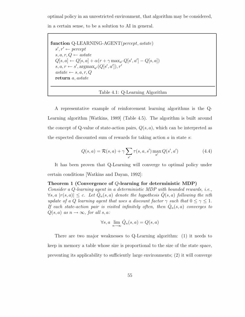
optimal policy in an unrestricted environment, that algorithm may be considered,
in a certain sense, to be a solution to AI in general.
function Q-LEARNING-AGENT(percept , astate)s′, r′ ← percepts, a, r, Q← astateQ[s, a]← Q[s, a] + α(r + γ maxa′ Q[s′, a′]−Q[s, a])s, a, r ← s′, argmaxa′(Q[s′, a′]), r′
astate ← s, a, r, Qreturn a, astate
Table 4.1: Q-Learning Algorithm
A representative example of reinforcement learning algorithms is the Q-
Learning algorithm [Watkins, 1989] (Table 4.5). The algorithm is built around
the concept of Q-value of state-action pairs, Q(s, a), which can be interpreted as
the expected discounted sum of rewards for taking action a in state s:
Q(s, a) = R(s, a) + γ∑
s′
τ(s, a, s′) maxa′
Q(s′, a′) (4.4)
It has been proven that Q-Learning will converge to optimal policy under
certain conditions [Watkins and Dayan, 1992]:
Theorem 1 (Convergence of Q-learning for deterministic MDP)Consider a Q-learning agent in a deterministic MDP with bounded rewards, i.e.,∀s, a |r(s, a)| ≤ c. Let Qn(s, a) denote the hypothesis Q(s, a) following the nthupdate of a Q learning agent that uses a discount factor γ such that 0 ≤ γ ≤ 1.If each state-action pair is visited infinitely often, then Qn(s, a) converges toQ(s, a) as n→∞, for all s, a:
∀s, a limn→∞
Qn(s, a) = Q(s, a)
There are two major weaknesses to Q-Learning algorithm: (1) it needs to
keep in memory a table whose size is proportional to the size of the state space,
preventing its applicability to sufficiently large environments; (2) it will converge
55

only for an environment that is fully observable, i.e., when it has complete in-
formation about the environment. Obviously, in the real world, these conditions
are rarely met.
4.6 Incomplete Information
There are compelling reasons that agents may not have complete information
about the environments:
1. The environments of interest are usually much larger, more complex thanthe agents in them, so it is not always possible to store all the information.
2. The environment may contain several agents, each of whose internal statesare not accessible by other agents.
3. Even in the cases where it is possible, it may not be desirable; e.g., storinginformation that is not critical to decision making may slow down accessto important information because of indexing overhead, resulting in lowerperformance.
4. In the physical world, information about the world can only be acquiredthrough sensors; and there are physical limits to how much information thesensors can sense.
5. The physical laws may be subtle or even intrinsically non-deterministic.
As a result, dealing with incomplete information is an issue inevitable to intelli-
gent agents.
Consider the grid world depicted in Figure 4.3, where, for the purpose of viv-
ifying the difficulties caused by incomplete information, we limit the perception
of the agent to its immediate surrounding. An optimal policy would follow the
diagonal line to visit the black dots. However, a Q-Learning algorithm will not
be able to learn the policy: to go from one black dot to another, the agent will
need go through a sequence of locations which are indistinguishable to its limited
56

ffffffffffff
ffffffffffff
ffffffffffff
ffffffffffff
ffffffffffff
ffffffffffff
ffffffffffff
ffffffffffff
ffffffffffff
ffffffffffff
ffffffffffff
ffffffffffff
v
v
v
v
j��
@@
@@
��
Figure 4.3: A 12× 12 toroidal grid world, wherethe world is not fully observable by the agent:the perception of the agent is limited to its ownlocation and the four immediate neighbors (in-dicated in the figure by points bounded by thebox around the agent). The black points aredistributed according to the equations y = x, ymod 3 = 0, where x, y ∈ Z.
perception, yet to implement the diagonal policy, it will need to perform different
actions in some of these indistinguishable states.
For example, let’s suppose the agent is moving from the second black dot to
the next one in the upper-right direction. One optimal policy is for it to move
three times to the right, and then three times up. When the agent is in the
location indicated in Figure 4.3, the policy dictates that it should move right;
after that, it should move up; but that is impossible for the Q-learning agent
since its percept is the only thing it uses to decide the next action, and the
percepts in those two location are the same.
4.7 Partially Observable Markov Decisions Processes
When the environment is only partially observable, the agent would not be able
to determine with certainty which state it is in; a policy that decides the next
action purely by looking at the current percept would clearly be inadequate.
When the designer of an agent can acquire sufficient knowledge about the
environment, consisting of knowledge about (1) the state transition model (in the
form of probability distribution when the environment is indeterministic); and
(2) the observation model specifying the probability of underlying environment
57

state given the observed state; then optimal decision making and acting in such
environment can be modeled as a Partially Observable Markov Decision Process
(POMDP) [Sondik, 1971, Lovejoy, 1991].
Formally, a POMDP consists of seven components, 〈S, C,O,R, β, φ, τ〉. They
are, respectively,
• States : a set S;
• Action: a set C;
• Observation: a set O;
• Reward function: a function R : S → ℜ;
• Initial state probability distribution: β : S → [0, 1];
• Observation probability distribution: φ : S × C × O → [0, 1];
• Transition probability distribution: τ : S × C × S → [0, 1].
It has been observed that POMDPs can be transformed into a regular MDP
(albeit over an infinite state space) by using the belief state [Astrom, 1965]. Based
on this observation, many algorithms have been proposed [Cassandra et al., 1994,
McCallum, 1995, Hansen, 1998, Pineau, 2004]. With the exception of the UTree
algorithm [McCallum, 1995], most algorithms for solving POMDPs require the
knowledge of the underlying environments. The UTree algorithm adopts the so-
called history-based approach, which use the history of action-perception pairs
to differentiate hidden states. For example, when faced with the scenario shown
in Figure 4.3 (discussed in Section 4.6), UTree algorithm would be able to use
the memory of how many steps the agent has taken after leaving one black dot
to choose appropriate actions during the sequence of perceptually identical states
between black dots. However, although the UTree algorithm has been empirically
shown to work well in certain cases, there is a deficiency. For example, consider
58

ffffffffffff
ffffffffffff
ffffffffffff
ffffffffffff
ffffffffffff
ffffffffffff
ffffffffffff
ffffffffffff
ffffffffffff
ffffffffffff
ffffffffffff
ffffffffffff
vv
v
j��
@@
@@
��
Figure 4.4: A 12× 12 toroidal grid world, wherethe black dots are distributed indeterministicallywith probability 0.2 on the line specified by theequations y = x, where x, y ∈ Z.
the instance of grid-world in Figure 4.4 where the black dots are scattered inde-
terministically according to some probability distribution. The distances between
two black dots can be arbitrary large, rendering the history-based approach in-
effective.
4.8 Bounded Optimal Rationality
For any fully observable MDP, a reactive control policy (i.e., one whose action
recommendation completely depends on the current percept) is sufficient for op-
timal behavior, so an optimal policy in such environment can be assumed to be
the “best possible” in practice: the policy can be implemented as simple table
lookup, which is practically a constant time operation, for example, by using a
hash table.
However, this is not the case for an POMDP, where, to estimate the best
action, an optimal policy would usually need to perform certain kind of search,
which takes an indefinite amount of time. Spending more time in searching may
find a better action, but would increase the risk of losing track of the changes
in world; so there is a fundamental trade-off involved here. What is the “best
possible” policy is less clear in this setting.
59

One good starting point for identifying a performance measure is the notion
of Bounded Optimality proposed by Russell et al. [Russell and Subramanian,
1995], which defines the optimality of the performance of a bounded agent with
respect to the physical characteristics (e.g., processor speed, memory space) of
the machine on which the agent is implemented) and a fixed environment:
Definition 1 (Russell’s Bounded Optimal Rationality) Definef = Agent(l, M) to be an agent function implemented by the program lrunning on machine M . Then the bounded optimal program lopt is defined by
lopt ≡ argmaxl∈LMV (Agent(l, M),E, U)
where LM is the finite set of all programs that can be run on M ; E is the en-vironment in which the agent is to operate, and U is the performance measurewhich evaluates the sequence of states through which the agent drives the actualenvironment; V (f,E, U) denotes the expected value according to U obtained byagent function f in environment class E, which is assumed to be a probabilitydistribution over elements of E.
A few remarks:
1. Observe that the bounded optimal agent is dependent on the environment;
intuitively, an agent specially trained to a specific environment will perform
better than others.
2. The design of an agent adapted to one environment will be quite different
from another (and the design process itself will likely take a lot of time
and resources); a design that can generalize and amortize the cost will be
desirable;
3. A BO agent is a function of the complete specification of a environment;
that is not likely to be available to the designer in most cases.
Because of the dependence on the fixed environment specification, Bounded
Optimality is not directly applicable to a non-stationary environment.
60

4.9 Non-stationary Environment
In every model or example environment we have discussed so far, the agent de-
signed is the only cause of changes in the world. More generally, we have been
assuming the rules governing the dynamics of the environment do not change.
The world we are living in obviously does not fit such an assumption.
A stationary process is a process of change that is governed by laws that
do not themselves change over time. Since the real world is non-stationary, it
would seem any agent that aspires to the claim of intelligence must be able to
deal with non-stationary environments adequately. However, it is much less clear
what would constitute a good performance measure in such environments. It is
not even clear learning would be possible (We will discuss this point further in
Section 4.10).
To develop an intuition of the difficulty, we again look at the grid-world. With
the stationary assumption, the distribution of the black dots in the world can be
specified by a characteristic function of two variables (namely the x, y coordinates
of the black dots), K : X × Y → {0, 1}; X, Y ⊆ Z, which returns 1 when the dot
corresponding to the pair of coordinates is black, and 0 otherwise. Without the
stationary assumption, the characteristic function will be of three parameters,
with the third parameter being the time (see Figure 4.5 for an example): K :
X × Y × T → {0, 1}
4.10 Intelligence in General
When an agent does not make any assumption about the “physics” of the envi-
ronment, then the agent can be seen as a universal agent, since it can then work
61

ffffffffffff
ffffffffffff
ffffffffffff
ffffffffffff
ffffffffffff
ffffffffffff
ffffffffffff
ffffffffffff
ffffffffffff
ffffffffffff
ffffffffffff
ffffffffffff
v v
v v
v v
v v
v v
v v
jffffffffffff
ffffffffffff
ffffffffffff
ffffffffffff
ffffffffffff
ffffffffffff
ffffffffffff
ffffffffffff
ffffffffffff
ffffffffffff
ffffffffffff
ffffffffffff
v v
v v
v v
v v
v v
v v
j
Figure 4.5: A non-stationary toroidal grid world, where the positions of blackpoints move up a step for each time step. The two figures depict snapshots ofthe world when t = 0 and t = 1, respectively. The black points are distributedaccording to the equations (y − 2x − t) mod 12 = 0, where x, y, t ∈ Z, and t isthe time step number.
equally well (or badly) in every environment. Does an optimal agent in such an
environment exist? To answer this question, we need to overcome at least two
problems: (1) What can we assume about the universal environment? (2) What
does optimal mean in such an environment?
Looking at the example in Section 4.9, when K is the random function, obvi-
ously no learning would be possible, and every agent would perform as well (or
as badly) as any other on average. Therefore it seems justified to hypothesize
that
Conjecture 1 Learning, hence intelligence, is not always possible in all envi-ronments.
and,
Conjecture 2 Intelligence is closely related, and relative, to environments.
Intuitively, the simpler K is, the faster should it be possible for an agent to
learn and converge to optimal behavior in that environment. The observation
leads to the following conjecture:
62

Conjecture 3 The most intelligent universal agent is the one whose rate oflearning is proportional to the algorithmic complexity of the environment.
Kolmogorov algorithmic complexity seems to be of particular relevance here:
Definition 2 (Kolmogorov’s Algorithmic Complexity) The conditionalprefix Kolmogorov complexity C of x given a sequence y is defined as the shortestprogram p, for which a universal Turing machine U outputs x given y:
C(x|y) ≡ minp{(l(p) : U(p, y) = x)}
If we regard the universal environment as the one such that all possible envi-
ronments may occur in time, we can make no assumption about the environment;
therefore we may also call it the null environment. However, even in such an envi-
ronment, there seems to be a natural structure imposed by algorithm complexity.
That is the basic intuition behind Solomonoff’s universal prior [Solomonoff, 1964,
1978]:
Definition 3 (Solomonoff’s Universal Prior) The universal prior M of asequence x is defined as the probability that the output of a universal Turingmachine starts with x:
M(x) ≡∑
p:U(p)=x∗
2−l(p)
The so-called “Universal AI” proposed by Hutter [Hutter, 2005] is based on
the universal prior, and he has proof showing that his “algorithm” is optimal
in the universal environment. Unfortunately, universal prior is undecidable, so
the “algorithm” has no practical application, and is not strictly an algorithm
according to the conventional definition of “effective procedure that terminates
in finite number of steps.” It remains to be seen if it is possible to “scale down”
his method to a practical algorithm for an agent with bounded resources while
retaining the property of optimality.
In this thesis, we are attacking the problem from the opposite direction: we
start from boundedness, and seek ways to approach optimality. We can at least
be ensured of retaining the boundedness.
63

4.11 Discussion
It has been a long debate among AI researchers on how much knowledge is needed
for the agent to be able to evolve in “interesting” environments. In general, the
less prior knowledge is assumed, to more environments will the agent be adapted;
however, the price of the generality will be the efficiency; the less is specified, the
more the agent has to figure out. In the case of a learning agent, the more time
will it take for the agent to adapt.
For example, an agent that has a statistical model of the world, by using
Bayesian reasoning, etc. will perform better than one without. However, this
doesn’t mean we need to specify the agent in these concepts directly; it is pos-
sible that we can get away with it by just specifying the axioms of probability.
The question is how to choose the appropriate level of details to make the boot-
strapping faster. To answer this question, perhaps we need to apply to ourselves
similar analysis that we are applying to the designing of the agent. This may
be seen as an optimization problem: obviously, some prior knowledge is needed;
but accumulating and encoding world knowledge for an agent’s consumption is
an expensive, difficult and tedious task for human being. How much knowledge
will be optimal in the sense of exploiting the different characteristics of a human
and a computer for processing knowledge?
4.12 Conclusions
This chapter is mainly to set the stage for the subsequent chapter, by introduc-
ing the necessary background. In particular, we described a series of increasingly
general (or less restrictive) models of environments, and discussed possible per-
64

formance measures and algorithms for solving them. We put forward a few con-
jectures on general intelligence, i.e., an optimal algorithm for agent in universal
environment. In future work, we intend to make the conjectures more formally
rigorous. To develop a better understanding of the issues involved in the con-
jectures, we will propose an algorithm for a prototypical agent in a universal
environment in the next chapter.
65

Chapter 5
Reflective Reinforcement Learning
5.1 Overview
An agent is said to be rational if the actions it takes maximize the expectation
of success, given what it knows about the environment. In most environments,
rationality is not realizable since the time it takes for computing the best action
usually far exceeds the time available to issue an action to meet the changes in
the environment. Bounded rationality refines the notion of rationality by taking
the availability of computational resources (including time) into consideration.
[Russell and Subramanian, 1995] gives a mathematically rigorous formulation of
bounded optimal rationality which is by construction realizable or “feasible”,
given a model of the environment and some specification of the physical charac-
teristic of computational devices available to the agent. However, even though
we know an agent satisfying bounded optimal rationality exists given the above
conditions, we don’t know (yet) how to find that feasible agent or if finding it
will ever become “feasible” in realistic environment.
If we rise to the meta level and look at the whole problem composed of (a)
finding the feasible agent, and (b) solving of the (object) problem of maximizing
66

utility in the environment by the agent, an intriguing question arises: Is this
process of solving a task environment by separating it into the (sub)processes
of (1) finding a feasible agent, and (2) making the agent solve the task, itself
bounded optimal?
On the other hand, conventional reinforcement learning algorithms for par-
tially observable Markov-Decision-Processes (POMDPs) are often subdivided (ei-
ther conceptually, or sometime implementationally) into two parts: (1) main-
tenance of belief states from observations and state estimation; (2) finding or
approaching the optimal policy in the belief space. However, this subdivision
of labor presents some problems: e.g., the maintenance of belief states requires
computational resources and takes time; furthermore, in most (all?) existing
algorithms, determining the next action requires forward search in infinite be-
lief spaces that have exponential runtime. We are faced with the (meta-)task of
deciding how much resources to be appropriated for each component of the task.
Based on these observations, we develop the reflective Q learning (RQL) al-
gorithm that will adapt and specialize itself to the changing environment, by not
only using reinforcement learning for learning policy to adjust the environment,
but also to adjust the agent itself. In effect, an RQL agent can be seen as hav-
ing a meta-agent as a component, which treats the object-level agent as part of
its environment, thus subjected to reinforcement-based adjustment. From this
perspective, the object-level agent is responsible for reactive control, while the
meta-level agent is responsible for long-term deliberation on how to prepare the
object-level agent for better adaptation, and the two processes execute concur-
rently.
We rely on the convergence of conventional reinforcement learning algorithm
67

to ensure that the adjustments made will cause the whole system to gradually
optimize itself to bounded-optimality.
5.2 Problem Setting
AI research is concerned with three kinds of entities: environment E , designer H,
programmable machineM. Typically, the designer has some goal, i.e., preference
U for the environment to be in certain states, and would be interested in finding
program P to control the machine to help achieve the goal. The combination of
the machine and the program together specifies an agent A.
The objective of an AI researcher Hu could be understood as finding a general,
effective methodology Pu for the designer to design a program to make the most
effective use of the machine. Complications can arise, e.g., from finding the
balance between the two kinds of effectiveness — a more effective program may
require a design method that takes a long time to finish, making it overall less
effective.
In general, the designer would not have full access to the environment; i.e., the
designer could be either (i) without full knowledge about the transition model,
(ii) without full knowledge about the possible states, (iii) uncertain about the
current state of the environment.
5.3 Reflective Reinforcement
The premises of reinforcement learning (RL) and a bounded-optimal-rational
agent are basically the same: there is an autonomous agent interacting with
an environment; the agent receives information about the environment through
68

certain channels of perception, and has a set of actions that it can perform to
affect the environment. Recurrently, based on the input from its sensor and its
internal state, the agent would select an action to affect the environment in some
desirable way.
As shown in the previous chapter, in its basic form, the Q-Learning algorithm
is unable to deal with an infinite state space, since an essential requirement for its
convergence is infinitely repeated visits to all states and infinite amount of mem-
ory to store information about them. Various techniques have been developed to
mitigate this weakness, basically by clustering similar states together. However,
the successful application of these techniques are usually “labor intensive”, since
the clustering methods are domain dependent.
Here we propose an “internal state” approach to deal with the infinite world:
instead of learning actions based on the actual states of the environment, the
internal state approach instead learns the internal states of an agent, as well as
the external states.
5.3.1 Algorithm
The proposed algorithm, which we will call Reflective Q-Learning (RQL), is based
on the Q-Learning (QL) algorithm, where both the states and actions are decom-
posed into two components. In RQL, a state S consists of two parts, S = 〈P, M〉,
where P is a projection of the external world, which may be intuitively under-
stood as the perception of the agent; and M is the memory state of the agent.
An action A also consists of two parts, A = 〈E, I〉, the external and internal
action. The external action serves a similar role to the action in traditional re-
inforcement learning algorithm, i.e., to cause change in the environment, while
69

the internal action is used to manipulate the memory state. The memory state
M and internal action I together define a finite state machine F . If we label the
elements of each of the set with integer, the transition rule can simply be defined
as τ(m, a) = (m+ i(a)) mod |M |, where i(a) = ⌊a/|I|⌋, and |.| is the cardinality
of a set.
function REFLECTIVE-Q-AGENT(percept , astate)p′, r′ ← perceptp, m, a, r, Q← astateQ[〈p, m〉, a]← Q[〈p, m〉, a] + α(r + γ maxa′ Q[〈p′, τ(m, a′)〉, a′]−Q[〈p, m〉, a])a← argmaxa′Q[〈p′, τ(m, a′)〉, a′]p, m, r ← p′, τ(m, a), r′
astate ← p, m, a, r, Qreturn ae, astate
Table 5.1: Reflective Q-Learning Algorithm
The algorithm is a strict generalization of the QL (which can be considered
as RQL with one internal state), and it retains much of the basic structure of
QL. Hence, it is rather straight forward to adapt most techniques for improving
QL, such as eligibility trace, prioritized sweeping, etc, to RQL.
5.3.2 Remarks
The internal state approach has the following potential advantages:
1. One obvious merit of our approach is, as mentioned above, the general-
ization of Q-Learning algorithm to a problem with an infinite number of
states. In this regard, our approach is not very different from other state
reduction techniques, and it remains to be seen whether this approach can
perform better than these known techniques. An immediate advantage is
70
we don’t have to devise a separate clustering method to classify the state,
since it is accomplished as part of the learning process.
2. Internal states provide a flexible medium for experimenting with varia-
tions of the Q-Learning algorithm. For example, one common theme in Q-
Learning research is the determination of an appropriate parameter value
for ǫ, the “exploration” factor for different domains. One trick we can play
with the internal state approach is we can attach a different set of parame-
ter values for different states of the agent, so that we can have a state with
very high exploration factor, whose main responsibility will be to cause un-
predictable behaviors. Again, the determination of these is “automatic” as
part of the learning process in our framework.
3. This framework allows the conflation of strategies for dealing with spatial
and temporal variations in the world. A big challenge for the Q-Learning
algorithm is dealing with changes in the world: for an agent residing in a
dynamic world, the policy it learns from one situation may not be effective
in another, and more significantly, the learnt policy may even be a hindrance
for the agent to adapt to the new situation. We conjecture that the internal
state approach to Q-Learning will be able to capture regularities in changes
over time, as well as those caused by the sequence of moves in physical
states. In other words, we think the internal states approach has a built in
mechanism to deal with perturbation, by its ability to accomodate multiple
policies and freely mix them together through internal transitions.
Because of these flexibilities, the convergence might be much slower than the
standard approach. Only empirical data can decide whether our approach is
71

sound.
5.4 Implementation
We have designed and implemented a general protocol for simulating agents-
world interaction which allows succinct specification of a reinforcement learning
agent and its environment. The protocol consists of (1) an agent specification
language, (2) an environment specification language, (3) an API (Application
Programming Interface) specification for the simulators where arbitrary agent
and environment behaviors may be specified. The framework is object-oriented,
based on CLOS, the Common Lisp Object System, enabling fine-grained control
and customization of a set of prototype agents and environments defined in the
protocol. In this section we will provide a documentation of the protocol and a
brief description of the prototype agents and environments.
5.4.1 Protocol
The agent and the world are CLOS classes; to add a new agent and environ-
ment, it would be sufficient to specialize the classes and implement the following
functions:
Generic function transition (world action)
"Return a new state of the world after taking action. Side-effect: the
world is destructively modified."
Generic function sensor (agent world)
"Return a perceived state; i.e., translate the state of the world into
percept of agent; in general, there are states that cannot be discerned
from each other wrt the agent. The purpose is to model the incomplete and
uncertain information that real agents will need to deal with."
Generic function utility (agent world)
"Return an estimate of the desirability of world wrt the agent."
Generic function policy (agent percept reward)
"Return an action, given the current perceived state of the world. Side
72

effect: the internal state of agent will be updated. In principle, policy
should not access the world directly, but call the sensor and utility
function."
5.5 Toroidal Grid World
There are several common benchmarks for POMDPs, e.g., the maze world and its
variations [McCallum, 1995], John Muir Trail [Angeline et al., 1994, Collins and
Jefferson, 1991], partially observable pole balancing [Meuleau et al., 1999], etc.
However, all of the these assume a stationary environment, i.e., a fixed transition
model. To test for the effectiveness of algorithms in non-stationary environments,
we need a benchmarking framework that includes dynamic elements. Ideally,
this framework should allow us to easily vary and control aspects of interest
of the world, such as observability, stationarity, determinism, etc, as well as
smooth transition from simple to more complex, realistic environments. For
these purposes, we devise the “toroidal grid world”.
5.5.1 “Physics” of the World
The toroidal grid world is a n× n, two dimensional grid world. Each grid point
may assume one of two possible values, empty or solid. At any given time, the
agent is located at one of the grid points, (x, y), where 0 ≤ x, y < n. At each time
step, the agent makes an perception (input) and produces an action (output).
The perception of the agent is controlled by a parameter, the range r, such
that the input to the agent consists of the configuration of the grid points within
the r × r square surrounding the agent. (The world will be fully observable by
the agent if we set r = n, and partially observable when r < n).
73

The action produced by the agent has five possible values:
{left, right, up, down, nil}.
The first four actions cause the agent to be in the immediate adjacent square to
the respective directions, while the fifth is a “no-op” that does not cause change
in position. Whenever the agent visits a solid point, it is rewarded with 1000
units; otherwise, -1 unit (e.g., to signify energy spent). To prevent the agent
from staying at (or repeatedly visiting) the same solid point, we keep a fixed-
length queue of q most recently visited solid points, so that no reward is given
for visiting points on the queue.
The “state of the world” can be completely identified by the conjunction of
the agent’s location and grid configuration. For an n × n world, the state size
is n2 · 2n2
. (When n = 48, the smallest grid size used in simulations that will
be described below, the state size is over 10600; hence, even if the world is fully
observable, conventional algorithms for solving MDP are out of the question in
this domain.)
The configuration of the solid points on the grid can be compactly represented
by a characteristic function k, whose range is {0, 1}, indicating whether a grid
point is empty (0) or not (1). In the case where the world is stationary, the
function would have two arguments, the x and y coordinates; for dynamic world,
it would have an additional third argument as the time index. A nondeterministic
world can be obtained by using a nondeterministic characteristic function.
Intuitively, the “complexity” of the characteristic function determines the
“complexity” of the world, which in turn determines how hard it will be to find
a “solution”, for some appropriate notions of “complexity” and “solution” (e.g.,
possible candidates for which are algorithm complexity and bounded-optimal
74

policy (suitably generalized to non-stationary environment), respectively). Since
the complexity of the characteristic function can be up to Turing-completeness, a
solution to the world will need to be Turing-complete as well. Hence, this bench-
mark seems adequate in providing a framework for us to study environments from
the very simple (fully observable, deterministic, stationary, Markovian, etc) to ar-
bitrarily complicated (including all combinations of observability, determinism,
stationarity and Markovian property).
5.5.2 Experiment Settings
Agent Parameters
The RQL algorithm, to a large extent, is domain independent: it assumes very
little knowledge about the environment. For example, compared with most al-
gorithms in the POMDP framework, RQL doesn’t assume a given world model
nor an observation model; in other words, we need to provide neither knowl-
edge about the preconditions, effects, etc of actions, nor characteristics such as
accuracy or reliability of sensors of the agent.
In theory, the only thing that needs to be changed in order to adapt the RQL
algorithm to a particular domain (environment) is the number of actions, |C|,
available to the agent. However, in practice, the time to convergence of RQL
will be affected by the choice of values for a few parameters. Since RQL can be
considered a generalization of Q-Learning (which is RQL with one internal state),
all Q-Learning parameters still apply here: learning rate (α), discount factor (γ),
exploration factor (ǫ), and eligibility trace (λ). Besides these, RQL also has
an additional parameter: the number of internal states, |I|, which constitutes a
kind of upper limit on the complexity of the agent. Intuitively, a larger number of
75

internal states would enable the algorithm to handle more complex, hence a larger
class of environments; however, it would also require a longer training period to
learn the appropriate internal structures. Our simulations below confirm this
intuition.
Environment Parameters
Since RQL, like most reinforcement learning algorithms, includes an “explo-
ration” factor which makes it stochastic, repeated trials using a variety of param-
eters are necessary for empirical verification of its performance and robustness.
This section gives details about the parameters used in our empirical study.
Within the toroidal grid world, the behavior of the environment can be fully
characterized by a quadruple 〈n, r, q, k〉, signifying the grid-size, perceptual range,
queue length and the characteristic function, respectively, of the environment as
detailed in the previous section. In our simulations, the typical values for the
grid-size n are 48, 120, 240, 480 and 720. In the rest of this chapter, unless
specified otherwise, the values of r and q will be 3 and 32, respectively.
As mentioned earlier, even for the smallest size of 48, the number of possible
states is in the order of 10600, making conventional Q-learning algorithms, which
require an entry in memory for each distinct state, unsuitable for fully-observable
variation of this domain. However, if we restrict the range of perception to only
part of the environment (e.g., to only the r × r points around the agent), Q-
learning can have some success in certain settings — depending on the values
of r and k. Intuitively, Q-learning would do well when the environment is such
that it is possible for the agent to follow an optimal policy without retaining any
information about the past. We will use an example to demonstrate this in the
76

ffffffffffff
ffffffffffff
ffffffffffff
ffffffffffff
ffffffffffff
ffffffffffff
ffffffffffff
ffffffffffff
ffffffffffff
ffffffffffff
ffffffffffff
ffffffffffff
v v
v v
v v
v v
v v
v v
j
Figure 5.1: Simplified k0 (interval of 2).
following subsection.
In the toroidal grid world, the most important factor in deciding the nature
of the environment is the characteristic function k. In our simulation, we mainly
used three instances of k: k0, k1 and k2 as defined by the equations below:
k0(x, y, t) =
1 if [(y + 2x) mod n = 0] ∧ [y mod 8 = 0]
0 otherwise
(5.1)
k1(x, y, t) =
1 if [(y + 2x) mod n = 0] ∧ [random(8) = 0]
0 otherwise
(5.2)
k2(x, y, t) =
1 if [(3y + (x mod 5)2 + t) mod n = 0] ∧ [y mod 2 = 0]
0 otherwise
(5.3)
where n is the grid-size, and random(i) is a non-deterministic function that re-
turns a number in 0, . . . , i− 1 with equal chance each time it is invoked. (Hence,
in Equation 5.2, the clause random(8) = 0 will be true, on average, once every 8
times the characteristic function k1 is called to determine the existence of reward
at a point.)
Among the three, k0 is the simplest one; it is deterministic and stationary. In
77
effect, the clause (y + 2x) mod n = 0 in Equation 5.1 causes the solid points to
be distributed on lines with a slope of −2 that intersect the origin (0, 0) and its
diagonally opposite corner (n, n), whilst the clause y mod 8 = 0 means the solid
points occur once every 8 consecutive points on the lines (See Figure 5.1 for a
simplified version of the world induced by k0, where the interval is 2 instead of 8).
With a large enough field of perception (r), a corresponding environment will be
a fully observable MDP, and can thus be solved using conventional reinforcement
learning algorithms, in theory. A larger grid-size will render these algorithms
impractical in most cases, however.
In Equation 5.2, an additional element of complication is introduced, in the
form of the random(.) function, making k1, and hence the resulting environments,
non-deterministic.
The definition of k2 in Equation 5.3 introduces another complication by mak-
ing use of the time index (t), which so far has been ignored in the previous two
characteristic functions. Because of the occurrences of t in the definition, a re-
sulting environment will no longer be stationary. In other words, “rules” that
hold for one instant may no longer be true in the next, making it seemingly the
most challenging.
5.5.3 Deterministic Stationary Environment (k0)
As hinted above, in an environment induced by k0, if we let the range of perception
r to be large enough (e.g., r = 10) such that the next solid point along the line
is “within sight” of the agent when it visits one, then traditional Q-learning can
still converge to an optimal policy, even though the environment is not a fully
observable MDP.
78

Figure 5.2 and 5.3, which show the performances of ordinary Q-Learning and
RQL respectively, confirm our observation:
The drops in QL performance can be explained by the exploration factor,
which sometimes makes the agent wander away from the lines until the solid dots
fall out from the field of perception. When no solid dot is in sight, Q-learning
can do no better than random walk, since all states would be indistinguishable
from the perspective of the agent.
RQL converges slower in comparison, because of the overhead in maintaining
and learning the internal memory states. However, the extra memory makes it
less susceptible to wandering, since it can wander farther before losing track of
where it is.
Figure 5.4 and 5.5 show the performances when the range of the field of
perception is set to r = 3. In this case, Q-Learning fails altogether to pick up the
right behavior (see Section 4.6 for explanation), while RQL learns the optimal
policy successfully.
It is well known that the condition entailed by fully observable MDP is suffi-
cient for Q-Learning to converge to optimal policy; this experiment provides an
example where full observability is not necessary.
5.5.4 Non-deterministic Stationary Environment (k1)
To test the performance of RQL in nondeterministic environments, we carried out
simulations in environments induced by the characteristic function k1 (as defined
in Equation 5.2), where the rewards (solid points) are distributed nondeterminis-
tically, with 1/8 probability, on lines intersecting the two diagonal corners of the
grid, with slope -2.
79
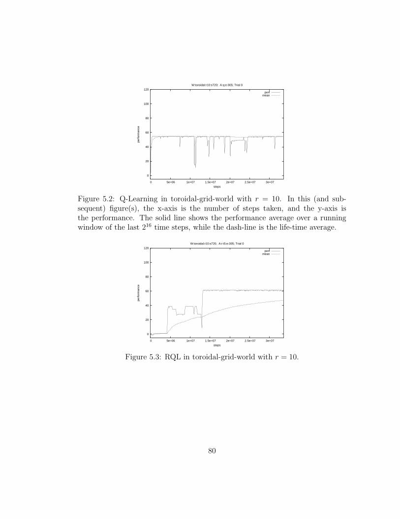
0
20
40
60
80
100
120
0 5e+06 1e+07 1.5e+07 2e+07 2.5e+07 3e+07
perf
orm
ance
steps
W:toroidal:r10:s720; A:q:e.005; Trial 0
perfmean
Figure 5.2: Q-Learning in toroidal-grid-world with r = 10. In this (and sub-sequent) figure(s), the x-axis is the number of steps taken, and the y-axis isthe performance. The solid line shows the performance average over a runningwindow of the last 216 time steps, while the dash-line is the life-time average.
0
20
40
60
80
100
120
0 5e+06 1e+07 1.5e+07 2e+07 2.5e+07 3e+07
perf
orm
ance
steps
W:toroidal:r10:s720; A:r:i5:e.005; Trial 0
perfmean
Figure 5.3: RQL in toroidal-grid-world with r = 10.
80

0
20
40
60
80
100
120
0 5e+06 1e+07 1.5e+07 2e+07 2.5e+07 3e+07
perf
orm
ance
steps
W:toroidal:r3:2x:s720; A:q:e.005; Trial 0
perfmean
Figure 5.4: Q-Learning in toroidal-grid-world with r = 3.
0
20
40
60
80
100
120
0 5e+06 1e+07 1.5e+07 2e+07 2.5e+07 3e+07
perf
orm
ance
steps
W:toroidal:r3:2x:s720; A:r:i5:e.005; Trial 0
perfmean
Figure 5.5: RQL in toroidal-grid-world with r = 3, using 5 internal states.
81

0
20
40
60
80
100
120
0 5e+06 1e+07 1.5e+07 2e+07 2.5e+07 3e+07
perf
orm
ance
steps
W:toroidal:r3:2x:chance:s720; A:r:i5:e.001; Trial 2
perfmean
Figure 5.6: Performance of RQL on an indeterministic toroidal grid world.
Clearly, for a large enough grid-size, the optimal policy would be for the agent
to follow the lines. Since it takes 3 steps at minimum to go from one point on the
line to the next (e.g., one step to the left and two steps down), thus the agent
needs to travel 3·8 = 24 steps on average to get one reward. Using a reward value
of 1000, this entails that the best average performance the agent can achieve is
(1000− 24)/24 ∼ 40.
To give a sense of the baseline performance to evaluate against, on a grid of
720 × 720 points, there is 1 reward per more than 5000 grid points — in other
words, a “brute-force” agent doing exhaustive search would get no better than
negative expected reward.
It is worth mentioning that in this setting, the distance between two rewards
can be arbitrarily large, making it hard for history-based or instance-based learn-
ing algorithms [McCallum, 1995].
Figure 5.6 shows the result of a trial on a 720× 720 grid. The figure shows,
in the form of the many “valleys” in the running window average performance
curve, similar periodic deterioration of performance due to the exploration factor,
which we also observed in the deterministic case (k0). The peaks do approach
82

the best possible performance of around 40, though; which means the optimal
policy had been attained, but then sometimes “forgotten”.
One obvious approach to diminish the forgetfulness, or the dips in perfor-
mance, is to employ simulated annealing technique to reduce the exploration
factor ǫ when sufficient performance is attained. However, we did not follow this
path for several reasons: first, even though in this particular case, we are able
to determine the optimal performance through analysis, in general, there has not
been known good way for the agent to assess its own performance and determine
whether it is close to optimum; second, even though it appears simulated an-
nealing would speed up convergence for stationary environment, we have reason
to believe it would hurt when the environment is non-stationary: The intuition
behind simulated annealing is to increase exploration, thereby learning, when not
much is known about the environment and hence performance is poor; but de-
crease exploration in order to increase exploitation of the learnt knowledge when
performance improves. However, in the case of a non-stationary environment, the
decrease in exploration would quite probably be detrimental to the adaptation of
the agent to the changed environment.
Instead of some ad hoc method for minor performance gain, we think these
simulation settings bring into focus much larger and interesting issues that call
for more systematic analysis and suggest many interesting questions: for exam-
ple, what are the meanings of the various parameters (such as ǫ, γ, etc that are
employed by various reinforcement learning algorithms) in non-stationary envi-
ronment? Would it be possible to find a universal, i.e., truly domain independent,
values for these parameters? Answering those questions will be a main part of
our future direction.
83

Average Performance over Repeated Trials
The nondeterminism in the environment, as well as the stochastic nature of the
algorithm, demand varied and repeated trials of the algorithm. Figure 5.7 to
5.9 show the results of simulations where we first varied the number of internal
states, and then the grid size. Each graph shows the average performance of 8
trials (see appendix for individual trials).
Figure 5.7 contains the outcome of the first batch of simulations, using a grid-
size of 48× 48, and k1 as the characteristic function. The six graphs are results
of the simulations where the numbers of internal states used are 1, 2, 3, 5, 10 and
20, respectively.
The first two graphs, where RQL is given 1 and 2 internal states respectively,
display little or no learning at all. This is not surprising: as mentioned earlier,
the optimal behavior in this environment is to follow certain lines with a slope of
-2. Because of the non-deterministic spacing between two consecutive rewards,
the agent needs to do this blindly, i.e., without relying on any distinction from
its perception while following the lines. Therefore, for the agent to realize the
behavior of going one step left and two steps down, it needs to keep track of
at least three states that correspond to the three steps routine. The rest of
the graphs confirm this observation: when RQL is provided with there or more
internal states, the required behavior is picked up somewhat successfully.
As noted earlier, the number of internal states represents a trade-off between
the capacity for complex behaviors and amount of training required for learning.
This is reflected in the slower learning rates shown in the last two graphs, where
10 and 20 internal states are used respectively.
The next two batches of simulations, whose outcomes are shown in Figure 5.8
84

and 5.9, where grid-sizes of 240 and 720 are used respectively, display similar
trend. (Closer examination of the first batch of graphs would reveal that the
performance of RQL in the 48×48 case appears to be inferior to the latter batches.
An explanation for that is local minimal: when the grid-size is comparatively
small, the agent may travel in direction perpendicular to the lines (i.e., with
slope 1/2) and still get above zero performance average.)
85

0
20
40
60
80
100
120
0 5e+06 1e+07 1.5e+07 2e+07 2.5e+07 3e+07
perf
orm
ance
steps
With 1 internal state
perfmean
0
20
40
60
80
100
120
0 5e+06 1e+07 1.5e+07 2e+07 2.5e+07 3e+07
perf
orm
ance
steps
With 2 internal states
perfmean
0
20
40
60
80
100
120
0 5e+06 1e+07 1.5e+07 2e+07 2.5e+07 3e+07
perf
orm
ance
steps
With 3 internal states
perfmean
0
20
40
60
80
100
120
0 5e+06 1e+07 1.5e+07 2e+07 2.5e+07 3e+07
perf
orm
ance
steps
With 5 internal states
perfmean
0
20
40
60
80
100
120
0 5e+06 1e+07 1.5e+07 2e+07 2.5e+07 3e+07
perf
orm
ance
steps
With 10 internal states
perfmean
0
20
40
60
80
100
120
0 5e+06 1e+07 1.5e+07 2e+07 2.5e+07 3e+07
perf
orm
ance
steps
With 20 internal states
perfmean
Figure 5.7: Static, nondeterministic, 48× 48 toroidal grid world.
86

0
20
40
60
80
100
120
0 5e+06 1e+07 1.5e+07 2e+07 2.5e+07 3e+07
perf
orm
ance
steps
With 1 internal state
perfmean
0
20
40
60
80
100
120
0 5e+06 1e+07 1.5e+07 2e+07 2.5e+07 3e+07
perf
orm
ance
steps
With 2 internal states
perfmean
0
20
40
60
80
100
120
0 5e+06 1e+07 1.5e+07 2e+07 2.5e+07 3e+07
perf
orm
ance
steps
With 3 internal states
perfmean
0
20
40
60
80
100
120
0 5e+06 1e+07 1.5e+07 2e+07 2.5e+07 3e+07
perf
orm
ance
steps
With 5 internal states
perfmean
0
20
40
60
80
100
120
0 5e+06 1e+07 1.5e+07 2e+07 2.5e+07 3e+07
perf
orm
ance
steps
With 10 internal states
perfmean
0
20
40
60
80
100
120
0 5e+06 1e+07 1.5e+07 2e+07 2.5e+07 3e+07
perf
orm
ance
steps
With 20 internal states
perfmean
Figure 5.8: Static, nondeterministic, 240× 240 toroidal grid world.
87

0
20
40
60
80
100
120
0 5e+06 1e+07 1.5e+07 2e+07 2.5e+07 3e+07
perf
orm
ance
steps
With 1 internal state
perfmean
0
20
40
60
80
100
120
0 5e+06 1e+07 1.5e+07 2e+07 2.5e+07 3e+07
perf
orm
ance
steps
With 2 internal states
perfmean
0
20
40
60
80
100
120
0 5e+06 1e+07 1.5e+07 2e+07 2.5e+07 3e+07
perf
orm
ance
steps
With 3 internal states
perfmean
0
20
40
60
80
100
120
0 5e+06 1e+07 1.5e+07 2e+07 2.5e+07 3e+07
perf
orm
ance
steps
With 5 internal states
perfmean
0
20
40
60
80
100
120
0 5e+06 1e+07 1.5e+07 2e+07 2.5e+07 3e+07
perf
orm
ance
steps
With 10 internal states
perfmean
0
20
40
60
80
100
120
0 5e+06 1e+07 1.5e+07 2e+07 2.5e+07 3e+07
perf
orm
ance
steps
With 20 internal states
perfmean
Figure 5.9: Static, nondeterministic, 720× 720 toroidal grid world.
88

0
20
40
60
80
100
120
0 5e+06 1e+07 1.5e+07 2e+07 2.5e+07 3e+07
perf
orm
ance
steps
W:toroidal:default:s720; A:r:i5:e.001; Trial 0
perfmean
Figure 5.10: Performance of RQL on a non-stationary toroidal grid world.
5.5.5 Non-stationary Environment (k2)
Figure 5.10 shows the result of a trial where the distribution of rewards is induced
by k2, which is non-stationary. In this case, there is one reward per 1450 grid
points on average.
Similar to the previous case, we ran multiple trials for each set of parameters
(Figure 5.11 to 5.13).
89

0
20
40
60
80
100
120
0 5e+06 1e+07 1.5e+07 2e+07 2.5e+07 3e+07
perf
orm
ance
steps
With 1 internal state
perfmean
0
20
40
60
80
100
120
0 5e+06 1e+07 1.5e+07 2e+07 2.5e+07 3e+07
perf
orm
ance
steps
With 2 internal states
perfmean
0
20
40
60
80
100
120
0 5e+06 1e+07 1.5e+07 2e+07 2.5e+07 3e+07
perf
orm
ance
steps
With 3 internal states
perfmean
0
20
40
60
80
100
120
0 5e+06 1e+07 1.5e+07 2e+07 2.5e+07 3e+07
perf
orm
ance
steps
With 5 internal states
perfmean
0
20
40
60
80
100
120
0 5e+06 1e+07 1.5e+07 2e+07 2.5e+07 3e+07
perf
orm
ance
steps
With 10 internal states
perfmean
0
20
40
60
80
100
120
0 5e+06 1e+07 1.5e+07 2e+07 2.5e+07 3e+07
perf
orm
ance
steps
With 20 internal states
perfmean
Figure 5.11: Dynamic 48× 48 toroidal grid world.
90

0
20
40
60
80
100
120
0 5e+06 1e+07 1.5e+07 2e+07 2.5e+07 3e+07
perf
orm
ance
steps
With 1 internal state
perfmean
0
20
40
60
80
100
120
0 5e+06 1e+07 1.5e+07 2e+07 2.5e+07 3e+07
perf
orm
ance
steps
With 2 internal states
perfmean
0
20
40
60
80
100
120
0 5e+06 1e+07 1.5e+07 2e+07 2.5e+07 3e+07
perf
orm
ance
steps
With 3 internal states
perfmean
0
20
40
60
80
100
120
0 5e+06 1e+07 1.5e+07 2e+07 2.5e+07 3e+07
perf
orm
ance
steps
With 5 internal states
perfmean
0
20
40
60
80
100
120
0 5e+06 1e+07 1.5e+07 2e+07 2.5e+07 3e+07
perf
orm
ance
steps
With 10 internal states
perfmean
0
20
40
60
80
100
120
0 5e+06 1e+07 1.5e+07 2e+07 2.5e+07 3e+07
perf
orm
ance
steps
With 20 internal states
perfmean
Figure 5.12: Dynamic 240× 240 toroidal grid world.
91

0
20
40
60
80
100
120
0 5e+06 1e+07 1.5e+07 2e+07 2.5e+07 3e+07
perf
orm
ance
steps
With 1 internal state
perfmean
0
20
40
60
80
100
120
0 5e+06 1e+07 1.5e+07 2e+07 2.5e+07 3e+07
perf
orm
ance
steps
With 2 internal states
perfmean
0
20
40
60
80
100
120
0 5e+06 1e+07 1.5e+07 2e+07 2.5e+07 3e+07
perf
orm
ance
steps
With 3 internal states
perfmean
0
20
40
60
80
100
120
0 5e+06 1e+07 1.5e+07 2e+07 2.5e+07 3e+07
perf
orm
ance
steps
With 5 internal states
perfmean
0
20
40
60
80
100
120
0 5e+06 1e+07 1.5e+07 2e+07 2.5e+07 3e+07
perf
orm
ance
steps
With 10 internal states
perfmean
0
20
40
60
80
100
120
0 5e+06 1e+07 1.5e+07 2e+07 2.5e+07 3e+07
perf
orm
ance
steps
With 20 internal states
perfmean
Figure 5.13: Dynamic 720× 720 toroidal grid world.
92

0
20
40
60
80
100
0 200000 400000 600000 800000 1e+06
mar
kers
foun
d
episodes
John Muir Trail
mean
Figure 5.14: Performance of RQL on John Muir Trail.
5.6 Other Experiments
5.6.1 John Muir Trail
John Muir Trail is a variation of the toroidal grid world, where a number of
markers are distributed on the grids according to a fixed scheme, forming a sort
of trail which might be broken, i.e., markers may be missing in some segments of
the trail. The task is to find as many marker as possible within a fixed number of
steps. Traditional studies of this problem use various techniques such as evolu-
tionary algorithm, neural networks, and sometimes the mix of the two [Angeline
et al., 1994]. In episodes of 512 maximal steps, the RQL algorithm is able to find
50 out of 89 of the markers after 40000 episodes, and all of them after around
750000 episodes (see Figure 5.14).
5.6.2 Partially Observable Pole Balancing
In the classical pole balancing task environment [Sutton and Barto, 1998], a pole
is hinged at one end to a cart that can move in both directions along a track of
93

some fixed length; the objective is to control the cart (by applying force in either
direction) to keep the pole from falling over while avoiding running off the track.
The relevant aspects of the environment can be represented as a four tuple
〈x, x, θ, θ〉, i.e., the position x and velocity x of the cart, and the angle θ and
angular velocity θ of the pole. Since the four components are continuous, this
environment has in theory an infinite number of states. A typical discretization
scheme is to divide each component into a small number of ranges; for example, a
program by Barto et al. [Barto et al., 1983] to simulate this environment divides
the four components into 3, 3, 6 and 3 discrete values respectively to obtain a total
of 163 (3× 3× 6× 3+1, where the 1 is the catch-all for all other possible values)
states. In such a setting, several well-known reinforcement learning algorithms
have been demonstrated to be able to ‘solve’ the task, i.e., to control the cart
successfully for over 100,000 steps after a number of trials.
The task becomes more challenging when some aspects of the state of the
environment are unobservable or suppressed, turning the task into a POMDP.
For example, Meuleau et al. [Meuleau et al., 1999] considers the pole balancing
task where only the position of the cart and the angle of the pole are observable,
while the knowledge of their velocities is missing.
Figure 5.15 shows the performance of our algorithm on the partially observable
pole balancing task. Meuleau et al. [Meuleau et al., 1999] indicated that they
subdivided the position and angle into finer discrete values (6 and 8 instead of
3 and 6 in Sutton’s original setting), but did not give detail on where they put
the cuts, so we are unable to reproduce the exact experiment. By inspecting the
figure in their paper, they attained an average performance of 600 steps in about
400000 trials. Even without the finer discretization, our algorithm attains 600
94

0
500
1000
1500
2000
2500
0 50000 100000 150000 200000 250000 300000 350000 400000
maxavg
Figure 5.15: Partially observable pole balancing. The x-axis represents the num-ber of trials (or episodes), and the y-axis the number of control steps attainedbefore failures. The pluses denote maximum values of 200 trials, while the solidline is the average.
steps of control in less than 250000 trials.
5.7 Summary
QL POMDP UTree RQL
FO Y Y Y Y
PO easy Y Y Y Y
PO hard N Y Y Y
PO rand N Y N Y
PO dyna N N ? Y
Table 5.2: Capabilities of various algorithms in different environments.
Table 5.2 is a summary of the capabilities of various algorithms. Below are
explanations of the labels:
FO: Fully observable.
95

PO easy: Partially observable, easy (e.g., where relevant features are within thefield of perception).
PO hard: Partially observable, hard (e.g., where relevant features are not withinthe field of perception).
PO rand: Partially observable, indeterministic.
PO dyna: Partially observable, non-stationary.
QL: Standard Q-Learning.
POMDP: The class of algorithms that require the knowledge of transition mod-els for the environments.
UTree: History (aka instance) based learning.
RQL: Reflective Q-Learning.
RQL seems to have a distinctive advantage in all the settings that have been
tried.
The one uncertainty is in the UTree case in the dynamic world. Ideally,
we should test it empirically using our setting, but we have not had success in
getting the McCallum’s UTree implementation [McCallum, 1995] to run. General
considerations of the nature of the algorithm suggest it might have trouble in a
dynamic setting. For instance, UTree will regard changes of positions of the solid
points as uncertainty in rewards that need to be resolved, and will split in an
effort to resolve it. One possibility is UTree will continue to split excessively
long as the rewards move around. A future work to consider is to empirically
investigate the performance of UTree in the dynamic setting.
5.8 Related Work
Designing agents in non-stationary environments has received little attention from
the AI community, where the “common wisdom” seems to be that, for an agent
96

to perform well in such an environment, it would need to solve many tasks that
have been proved computationally intractable, therefor impractical. The sub-
area that is closest to our work is research in POMDP. Among those, most
require the knowledge of the underlying transition models and observations of
the environment. The exceptions include the so-called history-based approaches.
History-based methods express policies conditioned on sequences of recent obser-
vations, instead of belief states. For example, the UTree algorithm [McCallum,
1995] offers an approach in which the observation histories are represented using
a suffix tree with variable depth leaves, and where branches are grown whenever a
new observation sequence is not Markovian with respect to the reward. The Pre-
dictive State Representation (PSR) approach [Littman et al., 2002, Singh et al.,
2003] is based on a similar premise, but instead of using history to condition
action-choices, the policy is conditioned on test predictions, where a test is a
sequence of future observations. In this approach, states are expressed in terms
of probabilities of observation sequences.
5.9 Conclusions and Further Work
It is generally believed that solving non-stationary environment is a difficult prob-
lem. Indeed, if “solving” means finding an optimal agent program, the problem is
intractable, and therefor impractical. However, being practical usually does not
require optimality; most of the time, it only needs to be good enough to survive,
or just a little bit better than the competition.
In this chapter, we introduced a new algorithm, RQL, for reinforcement learn-
ing in an unknown environment which may be time varying and non-stationary.
Experiments verified that the algorithm works well in situations not currently
97

known to be solvable or handled well by other existing algorithms.
One intriguing possibility is to see if it can be proved that RQL converges to
BOR for input sequence predictable by Solomonoff’s universal induction scheme.
RQL seems to have all the necessary ingredients of a bounded optimal agent:
the ability to acquire by learning an internal finite state machine, which is a
universal representation for any finite computing device. When put in a suitable
environment that can be marked by the agent, and hence serve as recording tape,
an RQL agent would be able in principle to learn the universal Turing machine;
so there is no lack of expressiveness in the representation. It has been discovered
that a POMDP can be reduced to an MDP over the infinite belief space. It seems
one possible direction to prove a convergence result is by identifying the internal
memory states learned by RQL with regions in the belief space. This will be one
important part of our future work.
98

Part IV
99

Chapter 6
Conclusions
6.1 Overview
Designing intelligent agents to perform well in realistic environment is an enor-
mously challenging task. Attempts at breaking down the problem may be put
into two categories: the top-down and the bottom-up approaches.
With the top-down approach, we model the problem by making some simpli-
fying assumptions and ignoring certain aspects of reality; e.g., we may advance
our understanding of computation by first constructing a model of computation
assuming the availability of infinite memory space, or infinite time. Examples of
this approach include the AIξ model of “Universal Artificial Intelligence” [Hutter,
2005], Universal Induction [Solomonoff, 1964, 1978], bounded optimality [Russell
and Subramanian, 1995], etc. Although the theories so constructed are general
and less susceptible to local minima than bottom-up bricks building, entities and
properties derived from them are usually non-constructively identified, rarely in-
forming procedural ways for achieving them. As a result, it is harder to design
concrete and practical algorithms from these theories.
With the bottom-up approach, we identify specific situations that agents may
100

encounter in the environment and design specific algorithms to deal with them;
the hope is that the more general situations can be solved by algorithms composed
of the various specific algorithm “bricks”. The majority of AI research such as
planning, automated theorem proving, machine learning, etc, may be put into
this category. This approach leads to sometimes practical algorithms but with
usually limited applicability. Moreover, it is non-obvious, or at least, not always
possible that there exists a composition of optimal algorithmic bricks that can
produce an optimal algorithm for more complicated situations.
The main goal of our research is to bridge this gap between theories and
practices. From one end, we start from POMDPs, one of the least restrictive
frameworks that has been more extensively studied, and seek to relax the few
requirements (e.g., the stationary constraint 1) assumed by existing algorithms.
From the other end, we use the notion of bounded-optimality as a guiding prin-
ciple for algorithm and agent design.
6.2 To the Future
Mathematicians stand on each other’s shoulders while computer
scientists stand on each other’s toes.
— Richard Hamming
We will see where we can go by first looking at what we have accomplished
so far (reproduced from Chapter 1):
1. The outline of a formal model of reflection based on the Belief, Desire,
1A stationary process is a process of change that is governed by laws that do not themselves
change over time.
101

Intention (BDI) agent model.
2. Preliminary design and implementation of a conversational agent based on
this model.
3. Design and implementation of computational-reflection inspired reinforce-
ment learning (RQL) algorithm that can successfully handle partially ob-
servable Markov decision processes (POMDPs) as well as non-stationary
environments.
4. Design and implementation of a novel benchmark problem which arguably
captures all the essential and challenging features of an uncertain, dynamic,
time sensitive environment.
5. Empirical studies of the comparative performances of RQL and some exist-
ing algorithms on the new and some well-known benchmark problems; this
includes the implementation of the RQL algorithm, benchmarks, and the
design and implementation of a general protocol for simulating agents-world
interaction.
6. Setting the stage for clarification of the relationship between bounded-
optimal rationality and computational reflection under the universal en-
vironment as defined by Solomonoff’s universal prior.
Among these, Reflective Q-Learning is the most intriguing. Experiments have
shown that it is rather competitive in well-known benchmark problems; however,
its more important role may be to serve as a prototype for investigation in possi-
ble ways to approach optimality in a general, unrestricted environment. An RQL
agent has the basic form (as a finite state machine) as well as the operation rule
102

(Bellman update) suggested by the definition of Bounded-Optimal-Rationality
(BOR), which, although not directly applicable to non-stationary environment,
should be a good starting point for a rigorous performance measure of an intel-
ligent agent. Even if we fail in our proof, the cause of failure should shed much
light on the nature of general intelligence.
103

BIBLIOGRAPHY
James [F.] Allen. Recognizing intentions from natural language utterances. In
Michael Brady and Robert C. Berwick, editors, Computational Models of Dis-
course. MIT Press, 1983.
Michael L. Anderson and Donald R. Perlis. Logic, self-awareness
and self-improvement: The metacognitive loop and the problem of
brittleness. Journal of Logic and Computation, 15(1):21–40, 2005.
http://logcom.oupjournals.org/cgi/content/abstract/15/1/21.
P. J. Angeline, G. M. Saunders, and J. B. Pollack. An evolutionary algorithm that
constructs recurrent neural networks. IEEE Transactions on Neural Networks,
5(1), 1994.
Lilian Ardissono, Guido Boella, and Rossana Damiano. A plan-based model of
misunderstandings in cooperative dialogue. International Journal of Human-
Computer Studies/Knowledge Acquisition, 1998.
K. J. Astrom. Optimal control of markov decision processes with incomplete
state estimation. J. Math. Anal. Applic., 10:174–205, 1965.
J. A. Austin. How to Do Things with Words. Harvard University Press, 1962.
A.G. Barto, R.S. Sutton, and C.W. Anderson. Neuron-like adaptive elements that
104
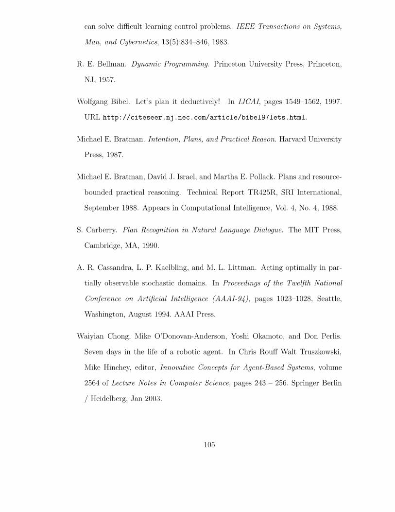
can solve difficult learning control problems. IEEE Transactions on Systems,
Man, and Cybernetics, 13(5):834–846, 1983.
R. E. Bellman. Dynamic Programming. Princeton University Press, Princeton,
NJ, 1957.
Wolfgang Bibel. Let’s plan it deductively! In IJCAI, pages 1549–1562, 1997.
URL http://citeseer.nj.nec.com/article/bibel97lets.html.
Michael E. Bratman. Intention, Plans, and Practical Reason. Harvard University
Press, 1987.
Michael E. Bratman, David J. Israel, and Martha E. Pollack. Plans and resource-
bounded practical reasoning. Technical Report TR425R, SRI International,
September 1988. Appears in Computational Intelligence, Vol. 4, No. 4, 1988.
S. Carberry. Plan Recognition in Natural Language Dialogue. The MIT Press,
Cambridge, MA, 1990.
A. R. Cassandra, L. P. Kaelbling, and M. L. Littman. Acting optimally in par-
tially observable stochastic domains. In Proceedings of the Twelfth National
Conference on Artificial Intelligence (AAAI-94), pages 1023–1028, Seattle,
Washington, August 1994. AAAI Press.
Waiyian Chong, Mike O’Donovan-Anderson, Yoshi Okamoto, and Don Perlis.
Seven days in the life of a robotic agent. In Chris Rouff Walt Truszkowski,
Mike Hinchey, editor, Innovative Concepts for Agent-Based Systems, volume
2564 of Lecture Notes in Computer Science, pages 243 – 256. Springer Berlin
/ Heidelberg, Jan 2003.
105

Phil Cohen. Dialogue modeling. In Ron Cole, Joseph Mariani, Hans Uszkoreit,
Annie Zaenen, and Victor Zue, editors, Survey of the State of the Art of Human
Language Technology, chapter 6.3. Cambridge University Press, Cambridge,
MA, 1996.
Philip R. Cohen and Hector J. Levesque. Communicative ac-
tions for artificial agents. In Proceedings of the First Interna-
tional Conference on Multi-Agent Systems, pages 65–72, San Fran-
cisco, CA, USA, 1995. The MIT PressCambridge, MA, USA. URL
http://citeseer.nj.nec.com/article/cohen95communicative.html.
Phillip R. Cohen and Hector J. Levesque. Confirmations and joint action. In
Proceedings IJCAI-91, pages 951–957, 1991.
Phillip R. Cohen and C. R. Perrault. Elements of a plan-based theory of speech
acts. Cognitive Science, 3(3):177–212, 1979.
P.R. Cohen, C.R. Perrault, and J.F. Allen. Beyond question answering. In
W. Lehnert and M. Ringle, editors, Strategies for Natural Language Processing,
pages 245–274. Lawrence Erlbaum, Hillsdale, 1981.
R. Collins and D. Jefferson. Artificial Life II, Santa Fe Institute Studies in
the Sciences of Complexity, volume X, chapter Antfarm: toward simulated
evolution. Addison Wesley, 1991.
S. Colton and A. Bundy. On the notion of interestingness in automated mathe-
matical discovery. In AISB Symposium on AI and Scientific Discovery, 1999.
D. Dennett. The Intentional Stance. MIT Press, Cambridge, MA, 1987.
106

J. Doyle. What is rational psychology, toward a modern mental philosophy. AI
Magazine, 4(3):50–3, 1983.
Michael R. Genesereth and Nils J. Nilsson. Logical foundations of artificial intel-
ligence. Morgan Kaufmann Publishers, Inc, 1988.
Barbara J. Grosz and Candace L. Sidner. Plans for discourse. In P. R. Cohen,
J. Morgan, and M. E. Pollack, editors, Intentions in Communication. MIT
Press, 1990.
R. Guha and Douglas Lenat. Cyc: a midterm report. AI Magazine, 11(3):32–59,
1990.
E. Hansen. Solving pomdps by searching in policy space. In Uncertainty in
Artificial Intelligence: Proceedings of the Fourteenth Conference, pages 211–
219, Madison, Wisconsin, 1998. Morgan Kaufmann.
E.J. Horvitz, J.S. Breese, and M. Henrion. Decision theory in expert systems
and artificial intelligence. International Journal of Approximate Reasoning, 2:
247–302, 1988.
Eric Horvitz. Models of continual computation. In Proceedings of the 14th Na-
tional Conference on Artificial Intelligence and 9th Innovative Applications of
Artificial Intelligence Conference (AAAI-97/IAAI-97), pages 286–293, Menlo
Park, July 1997. AAAI Press.
Eric Horvitz. Principles and applications of continual computation. Artificial
Intelligence, 126(1-2):159–196, March 2001.
Marcus Hutter. Universal Artificial Intelligence: Sequential Decisions Based on
Algorithmic Probability. Springer, Berlin, 2005. URL http://www.idsia.ch.
107

Darsana Joysula. A Unified Theory of Acting and Agency for a Universal Inter-
facing Agent. PhD thesis, University of Maryland, 2005.
Douglas B. Lenat. AM: Discovery in Mathematics as Heuristic Search, pages
1–225. McGraw-Hill, New York, NY, 1982.
Douglas B. Lenat. Theory Formation by Heuristic Search. Artificial Intelligence,
21:31–59, 1983.
Douglas B. Lenat and John Seely Brown. Why AM and EURISKO appear to
work. Artificial Intelligence, 23(3):269–294, 1984.
S.C. Levinson. The essential inadequacies of speech act models of dialogue. In
M. Parret, M. Sbisa, and J. Verschueren, editors, Possibilities and Limitations
of Pragmatics, pages 473–492. Benjamins, Amsterdam, 1981.
D. J. Litman and J. F. Allen. A plan recognition model for subdialogues in
conversation. Cognitive Science, 11:163–200, 1987.
M. L. Littman, R. S. Sutton, and S. Singh. Predictive representations of state. In
Advances in Neural Information Processing Systems (NIPS), volume 14, pages
1555–1561, Vancouver, 2002.
Karen E. Lochbaum. Using Collaborative Plans to Model the Intentional Struc-
ture of Discourse. Ph.d. dissertation, computer science department, Harvard
University, Cambridge, MA, 1994.
W. S. Lovejoy. A survey of algorithmic methods for partially observed markov
decision processes. Annals of Operations Research, 28(1-4):47–66, 1991.
108

Pattie Maes. Issues in computational reflection. In D. Nardi P. Maes, editor,
Meta-Level Architectures and Reflection, pages 21–35. Elsevier Science Pub-
lishers B.V. (North-Holland), 1988.
Andrew McCallum. Reinforcement Learning with Selective Perception and
Hidden State. PhD thesis, University of Rochester, 1995. URL
http://www.cs.rochester.edu/ mccallum/phd-thesis/.
John McCarthy. Artificial intelligence, logic and formalizing common sense. In
R. Thomason, editor, Philosophical Logic and Artificial Intelligence. Kluver
Academic, 1989.
Susan McRoy. Achieving robust human-computer communication. International
Journal of Human-Computer Studies, 48:681–704, 1998.
Susan W. McRoy and Graeme Hirst. The repair of speech act misunderstandings
by abductive inference. Computational Linguistics, 21(4):5–478, 1995.
Nicolas Meuleau, Leonid Peshkin, Kee-Eung Kim, and Leslie Kaelbling. Learning
finite-state controllers for partially observable environments. In Proceedings of
the 15th Annual Conference on Uncertainty in Artificial Intelligence (UAI-99),
pages 427–436, San Francisco, CA, 1999. Morgan Kaufmann Publishers.
R Montague. Syntactical treatments of modality, with corollaries on reflection
principles and finite axiomatizability. In Modal and Many-Valued Logics (Acta
Philosophica Fennica, vol. 16). Academic Bookstore, Helsinki, 1963. Reprinted
in R. Montague (1974). Formal Philosophy, New Haven, pp. 286-302.
K. L. Myers. User Guide for the Procedural Reasoning System. SRI International,,
Menlo Park, CA, 1997.
109

M. Nirkhe, S. Kraus, M. Miller, and D. Perlis. How to (plan to) meet a deadline
between now and then. Journal of logic computation, 7(1):109–156, 1997.
D. Perlis, K. Purang, and C. Andersen. Conversational adequacy: Mistakes are
the essense. International Journal of Human Computer Studies, pages 553–575,
1998.
Joelle Pineau. Tractable Planning under Uncertainty: Exploiting Structure. PhD
thesis, Robotics Institute, Carnegie Mellon University, Pittsburgh, PA 15213,
August 2004.
Anand S. Rao and Michael P. Georgeff. Modeling rational agents within a bdi-
architecture. In James Allen, Richard Fikes, and Eric Sandewall, editors, Pro-
ceedings of the Second International Conference on Principles of Knowledge
Representation and Reasoning (KR-91), pages 473–484, Cambridge, MA, May
1991.
Stuart Russell. Rationality and intelligence. Artificial Intelligence, 94(1-2):57–78,
July 1997.
Stuart Russell and Devika Subramanian. Provably bounded-optimal agents. Jour-
nal of Artificial Intelligence Research, 2, 1995.
Stuart J. Russell and Peter Norvig. Artificial Intelligence: A Modern Approach.
Prentice Hall, second edition edition, 2003.
H. Sacks, E. A. Schegloff, and G. Jefferson. A simplest systematics for the orga-
nization of turn-taking for conversation. Language, 50:696–735, 1974.
David Sadek and Renato De Mori. Dialogue systems. In R. De Mori, editor,
Spoken Dialogues with Computers. Academic Press, 1998.
110

John R. Searle. Speech Acts. Cambridge University Press, New York, 1969.
S. Singh, M. L. Littman, N. K. Jong, D. Pardoe, and P. Stone. Learning pre-
dictive state representations. In Machine Learning: Proceedings of the 2003
International Conference (ICML), pages 712–719, 2003.
Brian Cantwell Smith. Procedural Reflection in Programming Languages. PhD
thesis, Massachusetts Institute of Technology, 1982.
R. J. Solomonoff. Progress in incremental machine learning—preliminary report
for nips 2002 workshop on universal learners and optimal search. Technical
Report IDSIA-16-03, IDSIA, Lugano, 2003.
R.J. Solomonoff. A formal theory of inductive inference. Information and Control,
7:376–388, 1964.
R.J. Solomonoff. Complexity-based induction systems: comparisons and con-
vergence theorems. IEEE Transactions on Information Theory, 24:422–432,
1978.
E. J. Sondik. The Optimal Control of Partially Observable Markov Decision
Processes. PhD thesis, Stanford University, Stanford, California, 1971.
R.S. Sutton and A.G. Barto. Reinforcement Learning: An Introduction. MIT
Press, Cambridge, MA, 1998.
Michael Thielscher. Introduction to the fluent calculus. Linkoping Electronic
Articles in Computer and Information Science, 3(14), October 1998.
R Thomason. A note on syntactical treatments of modality. Synthese, 44:391–395,
1980.
111

D. Traum and E. Hinkelman. Conversation acts in task-oriented spoken dialogue.
Computational Intelligence, 8(3):575–599, 1992.
David R. Traum and James F. Allen. Discourse obligations in dialogue processing.
In Proceedings of the 32th Annual Meeting of the Association for Computational
Linguistics, pages 1–8, 1994.
J. von Neumann and O. Morgenstern. The Theory of Games and Economic
Behavior. Princeton Unversity Press, 1944.
C. J. C. H. Watkins. Learning from Delayed Rewards. PhD thesis, Cambridge
University, Cambridge, England, 1989.
C. J. C. H. Watkins and P. Dayan. Q-learning. Machine Learning, 8:279–292,
1992.
T. Winograd. Computer Models of Thought and Language, chapter A procedural
model of language understanding. Freeman, 1973.
David H. Wolpert and William G. Macready. No free lunch theorems for opti-
mization. IEEE Transactions on Evolutionary Computation, 1(1):67–82, April
1997.
112