Embed Size (px)
Citation preview
Abstract
PERRY, JOHN EDWARD. Combinatorial Criteria for Gröbner Bases. (Under
the direction of Hoon Hong.)
Both the computation and the detection of Gröbner bases require a criterion
that decides whether a set of polynomials is a Gröbner basis. The most funda-
mental decision criterion is the reduction of all S-polynomials to zero. However,
S-polynomial reduction is expensive in terms of time and storage, so a number
of researchers have investigated the question of when we can avoid S-polynomial
reduction. Certain results can be considered “combinatorial”, because they are cri-
teria on the leading terms, which are determined by integers. Our research builds
on these results; this thesis presents combinatorial criteria for Gröbner bases.
The first part of this thesis reviews the relevant literature on Gröbner bases and
skipping S-polynomial reduction. The second part considers criteria for skipping a
fixed number of S-polynomial reductions. The first two theorems of part two show
how to apply Buchberger’s criteria to obtain necessary and sufficient conditions for

skipping all S-polynomial reductions, and for skipping all but one S-polynomial
reductions. The third theorem considers the question of skipping all but two S-
polynomial reductions; we have found that this problem requires new criteria on
leading terms. We provide one new criterion that solves this problem for a set of
three polynomials; for larger sets, the problem remains open.
The final part of this thesis considers Gröbner basis detection. After a brief
review of a previous result that requires S-polynomial reduction, we provide a
new result which takes a completely different approach, avoiding S-polynomial
reduction completely.
Throughout the latter two parts, we provide some statistical analysis and ex-
perimental results.
8th April 2005
COMBINATORIAL CRITERIA FOR GRÖBNER BASES
BYJOHN EDWARD PERRY, III
A DISSERTATION SUBMITTED TO THE GRADUATE FACULTY OFNORTH CAROLINA STATE UNIVERSITY
IN PARTIAL FULFILLMENT OF THEREQUIREMENTS FOR THE DEGREE OF
DOCTOR OF PHILOSOPHY
DEPARTMENT OF MATHEMATICS
RALEIGH, NORTH CAROLINAAPRIL 2005
APPROVED BY:
H. HONGCHAIR OF ADVISORY COMMITTEE
E. KALTOFEN
A. SZANTO M. SINGER

Dedication
A Nonno Felice: guardando il nipote che leggeva, vide un professore.1
1Italian: To Nonno Felice: he looked at his grandson who was reading, and saw a professor.
ii

Biography
John Perry (III) was born in late 1971, in the city of Newport News, Virginia. His
parents are John Perry (Jr.), originally of Hampton, Virginia, and Maria Leboffe,
originally of Gaeta, Italy. Following graduation from Warwick high school, John
entered Marymount University. He graduated in 1993 with his B.S. in mathematics
and mathematics education. John subsequently earned an M.S. in mathematics
from Northern Arizona University. It was at this time that he began to experiment
with mathematics on the computer; one program that implemented the Runge-
Kutta interpolation to graph differential equations is available on-line for Amiga
computers: see [Per94].
After earning his master’s degree, John returned to Virginia and taught math-
ematics at Franklin County High School. Two years later, he volunteered for the
Catholic priesthood, but withdrew from seminary in December, 1998. He applied,
and was accepted, to North Carolina State University. He entered in the fall of 1999
and spent the next six years working on his doctorate.
iii

Acknowledgments
First, I must express my profound gratitude to the citizens of the state of North
Carolina, whose system of public universities is among the finest in the world. I
likewise thank the citizens of the United States, who supported my research in part
with NSF grant 53344.
I could never have hoped to be a doctoral student of mathematics at North
Carolina State University without both the inspiration and the instruction of past
teachers and professors. There is insufficient space to name them all, but I would
be remiss if I failed to name Neil Drummond, Vanessa Job, Judy Green, Adrian
Riskin (or Adrien Riskin, depending on his mood), Jonathan Hargis, and Lawrence
Perko.
I also thank the mathematics department at North Carolina State University, es-
pecially the computer algebra group, from whom I learned an immense amount. In
particular, my committee (Hoon Hong, Erich Kaltofen, Michael Singer, and Agnes
Szanto) taught excellent classes and looked at several incomplete drafts of this text.
iv
My advisor, Hoon Hong, spent countless hours guiding my research, teaching
me how to ask questions, how to answer them, and how to realize when the ques-
tion might be too hard. His advice and encouragement were invaluable. His wife
provided a number of delicious meals on many of the occasions that I passed the
hours with her husband hunched over a sheet of paper; on one occasion she drove
me to a car mechanic.
Erich Kaltofen provided a number of thoughtful conversations, not all about
mathematics. One of these conversations (on how mathematicians create ideas)
helped me realize that it was not yet time to abandon hope. He was always ready
with advice and information.
Bruno Buchberger suggested the statistical investigations of the results that ap-
pear at the end of chapter 6. Our discussions on the results of that chapter went a
long way towards deepening my understanding of them.
My officemates Chris Kuster, Alexey Ovchinnikov, Scott Pope, and George
Yuhasz were especially generous with their time and made a number of helpful
suggestions and contributions on papers, presentations, and this thesis.
Richard Schugart, my roommate of these past five years, has had to suffer my
quirky, a-social personality. He has put up with me much better than I proba-
bly would. His mother was very generous with cookies, for which I’m not sure
whether I owe her gratitude or grumbling – alas, my waistline has expanded.
v

My parents and my brothers have patiently endured my dissatisfaction with
personal and professional imperfections for thirty-three years now, and they have
never failed to challenge me to do my best. I come from a family privileged not
by wealth, but by the content of its character, to say nothing of the characters in its
contents. Ardisci e spera!2
Gal� nagradila ulybko$i na sem~ roz. 3
Finally: laus tibi, lucis largitor splendide.4
2A saying of my Italian grandfather and his brother: Dare and hope!3Galya rewarded seven roses with a smile.4Adapted from a medieval Latin hymn: Praise to you, O gleaming giver of light.
vi

Table of Contents
List of Figures ix
List of Tables xi
List of Symbols xiii
Part 1. Background Material 1
Chapter 1. An introduction to Gröbner bases 21.1. Gröbner bases: analogy 21.2. Gröbner bases: definition 71.3. Gröbner bases: decision 221.4. Some properties of representations of S-polynomials 48
Chapter 2. Skipping S-polynomial reductions 542.1. A Bottleneck 542.2. Skipping S-polynomial Reductions 552.3. Combinatorial Criteria on Leading Terms 582.4. The Buchberger Criteria 592.5. Term Diagrams 71
Part 2. New combinatorial criteria for skipping S-polynomial reduction 77
Chapter 3. Outline of part two 783.1. Buchberger’s criteria revisited 783.2. Formal statement of the problem considered in part two 803.3. Outline of the remainder of part two 823.4. An invaluable lemma 83
Chapter 4. Skipping all S-polynomial reductions 864.1. Problem 864.2. Result 874.3. Application of result 89
Chapter 5. Skipping all but one S-polynomial reductions 101vii
5.1. Problem 1015.2. Result 1025.3. Application of result 108
Chapter 6. Skipping all but two S-polynomial reductions (case for threepolynomials) 120
6.1. Problem 1206.2. Result 1236.3. Application of result 148
Part 3. A New Criterion for Gröbner Basis Detection of Two Polynomials 167
Chapter 7. Gröbner basis detection: introduction 1687.1. Introduction to the problem 1687.2. Matrix representations of term orderings 1717.3. Solving for admissible matrices 186
Chapter 8. Gröbner basis detection: general solution by polytopes 2008.1. Problem 2008.2. Polytopes, Polyhedra and Minkowski Sums 2018.3. Result 205
Chapter 9. Gröbner basis detection of two polynomials by factoring 2099.1. Problem 2099.2. Result 2099.3. Application of result 213
Conclusion 235
Bibliography 237
Index 241
viii

List of Figures
2.1 Term diagram of t1, t2, . . . , t6 722.2 Diagram of t1, t2, . . . , t6, with shading added for divisible terms. 732.3 Diagram of the greatest common divisor (lower left dot) and least common
multiple (upper right dot) of two terms. 742.4 Diagram of two relatively prime terms. 742.5 Diagram of the divisors (in grey box) that divide lcm (t4, t6). 752.6 No other monomial lies within the region of divisors of t1 and t2. 76
6.1 Diagram of proof strategy for section 6.2.3. 1276.2 Terms t1 and t3 have no indeterminates in common. 1526.3 Terms t1 and t3 have all their indeterminates in common. 1526.4 Terms t1 and t3 have one determinate in common. 1536.5 Theorem 6.3 allows a progression from Buchberger’s second criterion to
Buchberger’s first criterion. 1556.6 Ordering of critical pairs excludes most occurrences of the new criterion. 1616.7 Ordering of critical pairs excludes most occurrences of the new criterion. 1626.8 Ordering of critical pairs excludes most occurrences of the new criterion. 162
7.1 Diagram of vectors v1, v2 in example 7.8. 1817.2 How lemma 7.7 generates γ1, γ2 for example 7.8. 183
8.1 Newton polytope of f in example 8.2. 2028.2 Newton polyhedron of f in example 8.2 (first quadrant view only). 2028.3 The Minkowski sum of the Newton polytopes N (f) and N (g), from
example 8.5 2038.4 The Minkowski sum of the Newton polyhedra Naff (f) and Naff (g), from
example 8.5 2048.5 Normal cones of the Minkowski sum illustrated in figure 8.4. 205
ix

9.1 Summary of the number of detections of Gröbner bases for different casesof unstructured systems. 226
9.2 Summary of the number of detections of Gröbner bases for different casesof structured systems. 230
9.3 Detection compared to computation (chart of times): fixed number ofterms and fixed total degree. 231
9.4 Detection compared to computation (chart of times): 5% sparsity of termsand fixed total degree. 232
9.5 Detection compared to computation: fixed (chart of times): fixed numberof terms and increasing total degree. 233
x

List of Tables
4.1 Number of sets of polynomials where every pair of leading terms isrelatively prime, out of 100,000 sets. 95
4.2 Number of sets where every pair of leading terms is relatively prime, outof 100,000 sets. 95
4.3 Comparison of the number of Gröbner bases found by S-polynomialreduction, to the number found by applying theorem 4.1. 98
4.4 Comparison of the number of Gröbner bases found by S-polynomialreduction, to the number found by applying theorem 4.1. 99
5.1 Number of sets where we can skip all but one S-polynomial reduction, outof out of 100,000 sets. 115
5.2 Experimental results: number of sets, out of 100,000, where we can skip allS-polynomial reductions. 117
5.3 Comparison of the number of Gröbner bases found by S-polynomialreduction, to the number found by applying theorem 5.1. 118
6.1 Statistical analysis of new criterion on leading terms, assuming allS-polynomials reduce to zero. 158
6.2 Statistical analysis of new criterion on leading terms, assuming allS-polynomials reduce to zero. 158
6.3 Number of skips during the computation of a Gröbner basis for threerandomly-generated polynomials; total-degree term ordering. 160
6.4 Comparison of areas of regions: Buchberger criteria vs. new criterion(total-degree ordering). 164
6.5 Comparison of areas of regions: Buchberger criteria vs. new criterion(lexicographic ordering). 164
6.6 Which Si,j used r polynomials to reduce to zero (system 1). 1656.7 Which Si,j used r polynomials to reduce to zero (system 3). 1656.8 Which Si,j used r polynomials to reduce to zero (system 6). 165
xi

9.1 Number of times we detected a Gröbner basis for f1, f2 (six terms of totaldegree six). 224
9.2 Number of times we detected a Gröbner basis for f1, f2 (10% sparse, totaldegree 6). 225
9.3 Number of times we detected a Gröbner basis for f1, f2 (six terms of totaldegree 6×#vars). 226
9.4 Number of times we detected a Gröbner basis for gc1, gc2 (three terms ineach of g, c1, c2; maximum degree per term is 10). 227
9.5 Number of times we detected a Gröbner basis for gc1, gc2 (number ofterms in each of g, c1, c2 fixed at 5% sparsity, minimum two terms for c1, c2;maximum degree per term is 10). 228
9.6 Number of times we detected a Gröbner basis for gc1, gc2 (three terms ineach of g, c1, c2; maximum degree per term is 10×#vars). 229
9.7 Detection compared to computation: fixed number of terms and fixed totaldegree. 231
9.8 Detection compared to computation: fixed sparsity of terms and fixed totaldegree. 232
9.9 Detection compared to computation: fixed number of terms and increasingtotal degree. 232
xii

List of Symbols
Symbol page meaning
�,≺,�,� 9 term ordering
� 172 lexicographic ordering of a vector
−→,−→q·f
, 9 17 one-step reduction
∗−→(f1,...,fm)
,∗9
(f1,...,fm)17 complete reduction
55 can skip S-polynomial reduction
α(i) 172 row i of vector α
σij, σji 48 monomials used to construct Si,j
ω 187 weight vector
BC1 (t1, t3),BC2 (t1, t2, t3)
69 Buchberger’s first combinatorial criterion
CC 80 combinatorial criterion for skippingS-polynomial reductions
F 8 a field
F[x1, . . . , xn] the polynomial ring in x1, . . . , xn over F
GB� (f1, . . . , fm) 20 f1, . . . , fm are a Gröbner basis with respect to �
xiii

Symbol page meaning
I (f1, . . . , fm) 19 {h1f1 + · · ·+ hmfm : hk ∈ F[x1, . . . , xn]} (theideal of f1, . . . , fm)
M(i) 172 row i of matrixM
M(i,j) 189 row i, column j of matrixM
N (f) 201 the Newton polytope of f
Naff (f) 202 the Newton polyhedron of f
S� (fi, fj) 23 the S-polynomial of fi, fj with respect to �
Sfi,fj, Si,j 23 the S-polynomial of fi, fj with respect to a
given �
T (x1, . . . , xn) 9 the set of terms on x1, . . . , xn
VB1x (t1, t3),VB2x (t1, t2, t3)
123 variable-wise Buchberger criteria
xiv
Part 1
Background Material
Chapter 1
An introduction to Gröbner bases
1.1. GRÖBNER BASES: ANALOGY
This text studies certain properties of Gröbner bases. What are Gröbner bases?
We introduce them as an extension of a high-school topic.
1.1.1. A “NICE FORM”. Suppose we are given two polynomials f1, f2. We want to
know the following:1
• Do f1, f2 share any common roots?
• If so, is the solution set finite or infinite?
• If the solution set is finite, how many common roots are there?
• If the solution set is infinite, what is its dimension?
• Find or describe these common solutions.
1Although we raise these questions for the purpose of motivating the study of Gröbner bases, it isbeyond the scope of this text to answer them. The interested reader can find an excellent treatmentof these topics in [CLO97].
2

1.1. GRÖBNER BASES: ANALOGY 3
These are natural questions: systems of polynomials appear in numerous applica-
tions of mathematics, and the common roots of polynomial systems have impor-
tant real-world significance.
We would like a “nice form” that would help us answer these questions easily.
Such a “nice form” exists, and we call it a Gröbner basis.
The precise definition of a Gröbner basis will have to wait for section 1.2.4. For
now, we present an intuitive idea via two examples.
1.1.2. LINEAR POLYNOMIALS.
EXAMPLE 1.1. Consider the system
2x + 3y + 1 = 0
x + y = 0
Do the equations have common solutions?
High school students encounter this problems in Algebra I, and learn to solve
them by Gaussian elimination. They begin by writing the variables on one side, and
the constants on the opposite side:
2x + 3y = −1
x + y = 0
1.1. GRÖBNER BASES: ANALOGY 4
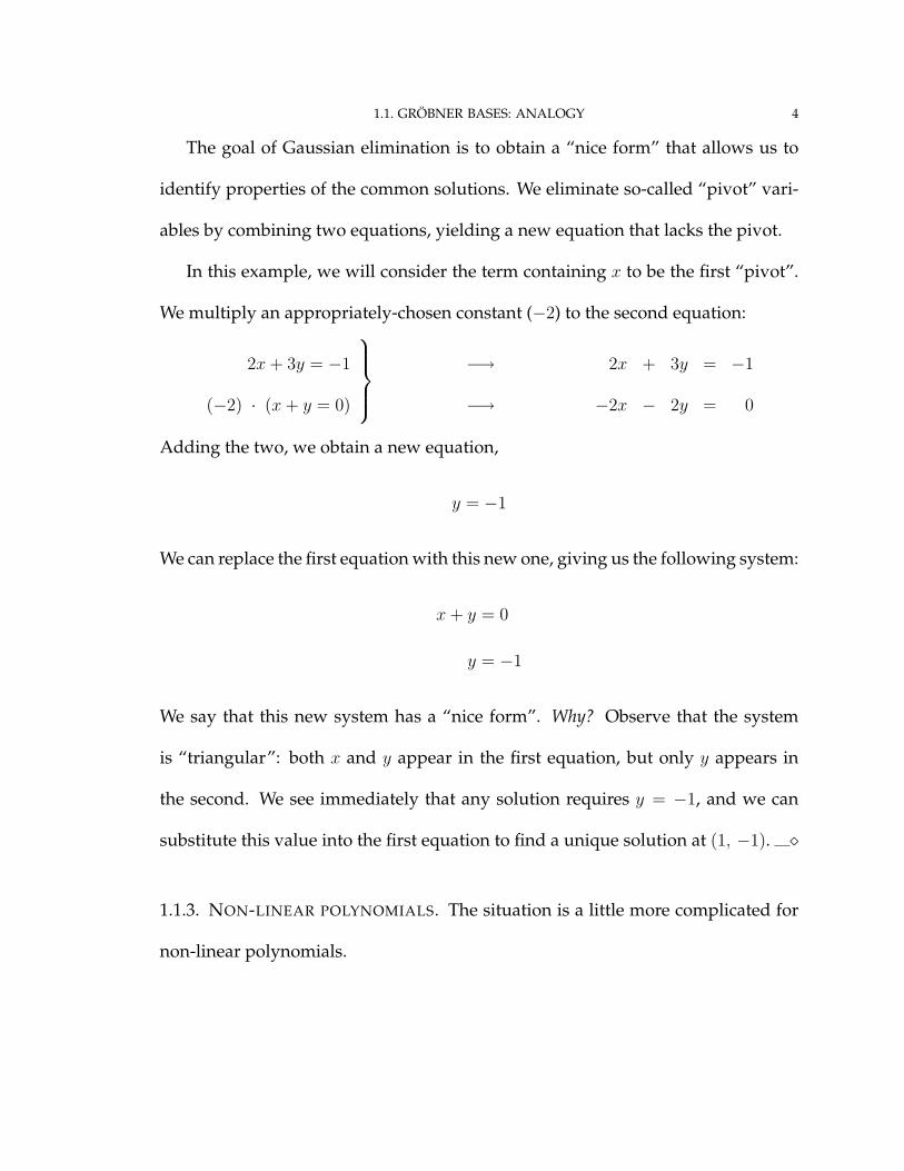
The goal of Gaussian elimination is to obtain a “nice form” that allows us to
identify properties of the common solutions. We eliminate so-called “pivot” vari-
ables by combining two equations, yielding a new equation that lacks the pivot.
In this example, we will consider the term containing x to be the first “pivot”.
We multiply an appropriately-chosen constant (−2) to the second equation:
2x + 3y = −1
(−2) · (x + y = 0)
−→
−→
2x + 3y = −1
−2x − 2y = 0
Adding the two, we obtain a new equation,
y = −1
We can replace the first equation with this new one, giving us the following system:
x + y = 0
y = −1
We say that this new system has a “nice form”. Why? Observe that the system
is “triangular”: both x and y appear in the first equation, but only y appears in
the second. We see immediately that any solution requires y = −1, and we can
substitute this value into the first equation to find a unique solution at (1, −1). �
1.1.3. NON-LINEAR POLYNOMIALS. The situation is a little more complicated for
non-linear polynomials.

1.1. GRÖBNER BASES: ANALOGY 5
EXAMPLE 1.2. Let
f1 = x2 + y2
f2 = xy
We want to know whether the system has a common root. This is equivalent to
saying that we want to know whether the equations
x2 + y2 = 0
xy = 0
have a common solution.
Perhaps we could generalize the method of example 1.1. Do these polynomials
have a “nice form”? If not, what must we do to find a similar ”nice form”?2
To answer the first question: no, this system is not a nice form.
So, we need to identify “pivots”. It doesn’t seem unreasonable to focus our
attention on the highest powers of x: so, we identify x2 and xy as “pivots” of
f1, f2.3
Now we want to eliminate the pivots. How? When the polynomials were linear,
the pivots were like terms, so we only needed to multiply by “magic constants.”
In this case, the pivots are not alike, so we need to multiply by monomials that give
2We do not yet have the machinery to provide the precise definition of this “nice form”; that willcome in definition 1.18 on page 19 of section 1.2.4.3There is a science of choosing pivots, and we provide a treatment of this science in section 1.2.2.
1.1. GRÖBNER BASES: ANALOGY 6
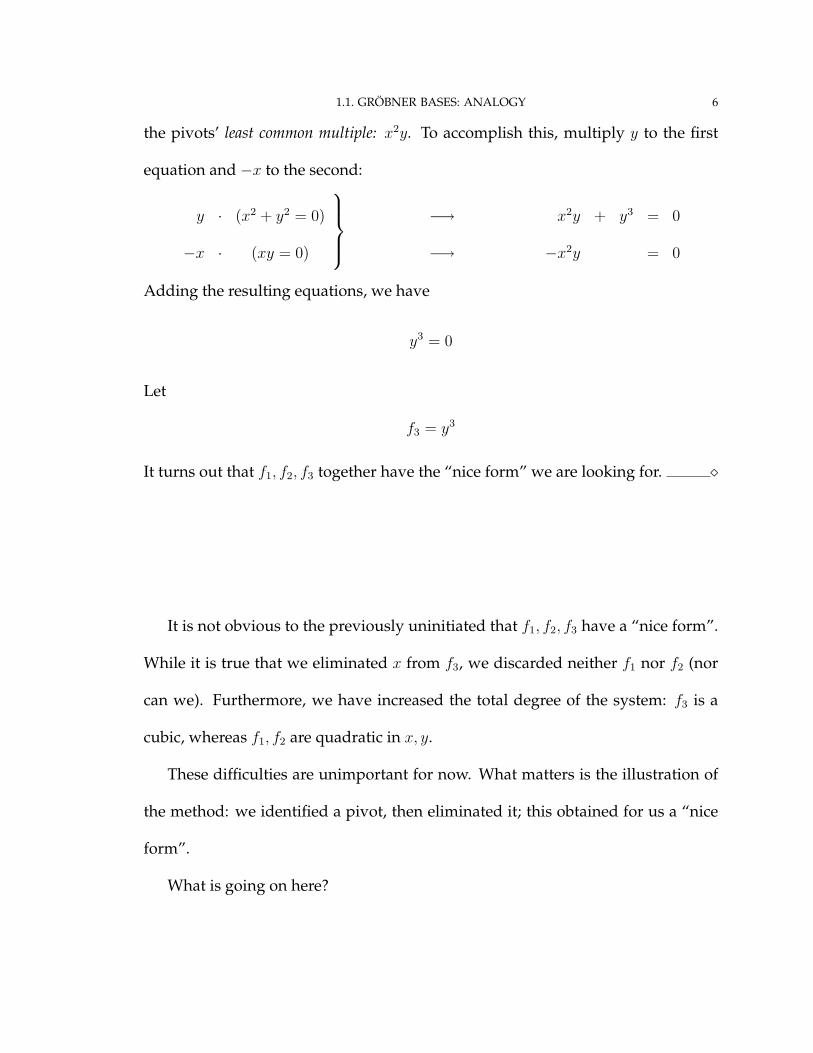
the pivots’ least common multiple: x2y. To accomplish this, multiply y to the first
equation and −x to the second:
y · (x2 + y2 = 0)
−x · (xy = 0)
−→
−→
x2y + y3 = 0
−x2y = 0
Adding the resulting equations, we have
y3 = 0
Let
f3 = y3
It turns out that f1, f2, f3 together have the “nice form” we are looking for. �
It is not obvious to the previously uninitiated that f1, f2, f3 have a “nice form”.
While it is true that we eliminated x from f3, we discarded neither f1 nor f2 (nor
can we). Furthermore, we have increased the total degree of the system: f3 is a
cubic, whereas f1, f2 are quadratic in x, y.
These difficulties are unimportant for now. What matters is the illustration of
the method: we identified a pivot, then eliminated it; this obtained for us a “nice
form”.
What is going on here?

1.2. GRÖBNER BASES: DEFINITION 7
1.2. GRÖBNER BASES: DEFINITION
In 1965 [Buc65] Bruno Buchberger invented an algorithm to compute such a
”nice form” for systems of polynomial equations. In honor of his advisor, Wolf-
gang Gröbner, he named this form Gröbner bases; the corresponding algorithm has
since become known as Buchberger’s algorithm. Gröbner bases are now recog-
nized as an important tool for describing solutions to systems of nonlinear equa-
tions. They form a part of all major computer algebra systems, and have found
their place as an important application to scientific research in fields such as physics
and engineering.4
A precise definition of a Gröbner basis appears in section 1.2.4; first, we must
establish some fundamental concepts.
1.2.1. TERMS, MONOMIALS, COEFFICIENTS. Different authors give incompatible
definitions to the notions of terms, monomials, and coefficients. We follow the
convention of the Maple computer algebra system.
4An on-line conversation with a cousin drove this point home to me. When he asked me what Iwas researching, I told him that I was working with Gröbner bases. To my surprise, my cousinreplied, “That sounds familiar... let me check.” I didn’t expect this, because he was a computerscience major, but a few moments later, he continued, “Yes, they’re in my astronomy book; they areused to compute singularities.”

1.2. GRÖBNER BASES: DEFINITION 8
DEFINITION 1.3. An indeterminate (also called a variable5) is an unspecified value.
A term is a product of indeterminates. A monomial is the product of a term and
a constant from the field F. We call this constant the coefficient. A polynomial is
the sum of a finite number of monomials.
EXAMPLE 1.4. Let
g = 5x2 − 3xy2 + y3
The monomials of f are
5x2 , −3xy2 , y3
The terms of f are
x2 , xy2 , y3
The coefficients of f are
5 , −3 , 1
�
1.2.2. TERM ORDERINGS (THE SCIENCE OF CHOOSING PIVOTS). Recall that in ex-
ample 1.2 we chose to eliminate the “pivots” x2 and xy. Why did we choose these
two monomials, rather than another pair, such as y2 and xy? We had chosen a term
ordering which identified x2 and xy as the “leading terms” of f1 and f2, respectively.
5Some authors distinguish between a variable and an indeterminate. For example, [Woo04] indi-cates that a variable has a solution, while an indeterminate does not. Other authors use the termsinterchangeably (for example, pg. 188 of [BWK93]). In any case, this distinction does not matterfor our purposes.
1.2. GRÖBNER BASES: DEFINITION 9
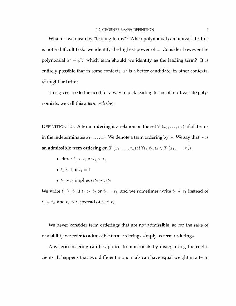
What do we mean by “leading terms”? When polynomials are univariate, this
is not a difficult task: we identify the highest power of x. Consider however the
polynomial x2 + y2: which term should we identify as the leading term? It is
entirely possible that in some contexts, x2 is a better candidate; in other contexts,
y2 might be better.
This gives rise to the need for a way to pick leading terms of multivariate poly-
nomials; we call this a term ordering.
DEFINITION 1.5. A term ordering is a relation on the set T (x1, . . . , xn) of all terms
in the indeterminates x1, . . . , xn. We denote a term ordering by �. We say that � is
an admissible term ordering on T (x1, . . . , xn) if ∀t1, t2, t3 ∈ T (x1, . . . , xn)
• either t1 � t2 or t2 � t1
• t1 � 1 or t1 = 1
• t1 � t2 implies t1t3 � t2t3
We write t1 � t2 if t1 � t2 or t1 = t2, and we sometimes write t2 ≺ t1 instead of
t1 � t2, and t2 � t1 instead of t1 � t2.
We never consider term orderings that are not admissible, so for the sake of
readability we refer to admissible term orderings simply as term orderings.
Any term ordering can be applied to monomials by disregarding the coeffi-
cients. It happens that two different monomials can have equal weight in a term

1.2. GRÖBNER BASES: DEFINITION 10
ordering, but this does not present a problem in practice; normally we combine
like monomials, and we will consider polynomials to be in this “simplified” form.
Let’s look at some common term orderings.
EXAMPLE 1.6. Let
g = 5x2 − 3xy2 + y3
One way to choose the leading terms would be by picking the higher power of x;
in case of a tie, we could fall back on the higher power of y. We can write this
formally as:
• lex (x, y): t1 �lex(x,y) t2 if
degx t1 > degx t2;
in the case that degx t1 = degx t2, if degy t1 > degy t2.
Another way to chose the leading terms would be by picking the higher power of
y; in case of a tie, we could fall back on the higher power of x. We can write this
formally as:
• lex (y, x): we say that t1 �lex(y,x) t2 if
degy t1 > degy t2;
in the case that degy t1 = degy t2, if degx t1 > degx t2.
We call�lex(x,y) and�lex(y,x) lexicographic term orderings (hence the label, lex). Con-
sider the terms x2, xy2, y3, 1; the former has
x2 �lex(x,y) xy2 �lex(x,y) y3 �lex(x,y) 1

1.2. GRÖBNER BASES: DEFINITION 11
and the latter has
y3 �lex(y,x) xy2 �lex(y,x) x2 �lex(y,x) 1
�
Of course, we need our term orderings to apply to terms in more than two in-
determinates. We can generalize the two term orderings of example 1.6 as follows:
DEFINITION 1.7. The lexicographic term ordering�= lex (x1, . . . , xn) gives t1 � t2
if
• degx1t1 > degx1
t2, or
• degx1t1 = degx1
t2 and
degx2t1 > degx2
t2, or
• . . .
• degx1t1 = degx1
t2 and
. . . and
degxn−1t1 = degxn−1
t2 and
degxnt1 > degxn
t2.
EXAMPLE 1.8. If �= lex (x, y, z), then
x2y2 � x2yz � xy2z � y3 � z5
As we noted above, we need term orderings to give us a precise manner of
choosing leading terms for multivariate polynomials.

1.2. GRÖBNER BASES: DEFINITION 12
DEFINITION 1.9. The leading term of a polynomial f = a1t1+· · ·+artr with respect
to a term ordering � is
max�{tk : k = 1, . . . , r}
that is, the term t such that t � u for every other term u of f . We write lt� (f) = t.
If the term ordering is understood from context, we write f = t.
The leading monomial of a polynomial f with respect to a term ordering � is
is the monomial containing f . We write m = lm� (f). If the term ordering is un-
derstood from context, we write f = m. The leading coefficient is the coefficient
of f in f , written c = lc� (f).
Note that
lm� (f) = lc� (f) · lt� (f)
or, if the term ordering is understood from context,
f = lc� (f) · f
Now let’s introduce a third term ordering, a total-degree term ordering. Here
we will pick the leading term not by favoring one variable over another, but by
favoring terms whose exponents have the highest sum. Before defining it precisely,
we’ll look first at an example in two variables.
1.2. GRÖBNER BASES: DEFINITION 13
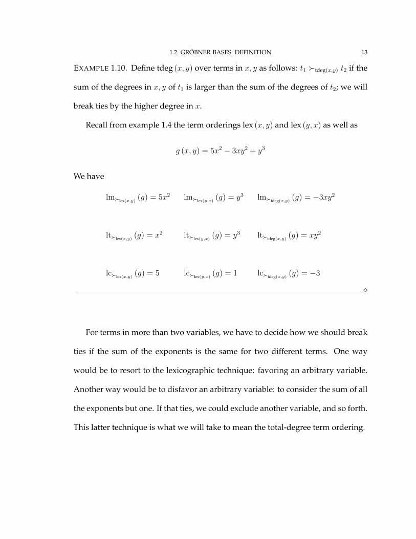
EXAMPLE 1.10. Define tdeg (x, y) over terms in x, y as follows: t1 �tdeg(x,y) t2 if the
sum of the degrees in x, y of t1 is larger than the sum of the degrees of t2; we will
break ties by the higher degree in x.
Recall from example 1.4 the term orderings lex (x, y) and lex (y, x) as well as
g (x, y) = 5x2 − 3xy2 + y3
We have
lm�lex(x,y)(g) = 5x2 lm�lex(y,x)
(g) = y3 lm�tdeg(x,y)(g) = −3xy2
lt�lex(x,y)(g) = x2 lt�lex(y,x)
(g) = y3 lt�tdeg(x,y)(g) = xy2
lc�lex(x,y)(g) = 5 lc�lex(y,x)
(g) = 1 lc�tdeg(x,y)(g) = −3
�
For terms in more than two variables, we have to decide how we should break
ties if the sum of the exponents is the same for two different terms. One way
would be to resort to the lexicographic technique: favoring an arbitrary variable.
Another way would be to disfavor an arbitrary variable: to consider the sum of all
the exponents but one. If that ties, we could exclude another variable, and so forth.
This latter technique is what we will take to mean the total-degree term ordering.

1.2. GRÖBNER BASES: DEFINITION 14
DEFINITION 1.11. The total-degree term ordering6 �= tdeg (x1, . . . , xn) gives t1 �
t2 if
• degx1t1 + · · ·+ degxn
t1 > degx1t2 + · · ·+ degxn
t2, or
• degx1t1 + · · ·+ degxn
t1 = degx1t2 + · · ·+ degxn
t2 and
degx1t1 + · · ·+ degxn−1
t1 > degx1t2 + · · ·+ degxn−1
t2, or
• . . .
• degx1t1 + · · ·+ degxn
t1 = degx1t2 + · · ·+ degxn
t2 and
degx1t1 + · · ·+ degxn−1
t1 = degx1t2 + · · · degxn−1
t2 and
. . . and
degx1t1 + degx2
t1 = degx1t2 + degx2
t2 and
degx1t1 > degx1
t2.
Let’s consider one last example to clarify how the total-degree term ordering
behaves with more than two indeterminates:
EXAMPLE 1.12. Let �= tdeg (x, y, z). Then
z5 � x2y2 � x2yz � xy2z � y3
Notice that in some cases, the ordering of the terms is the same as in example 1.8:
x2y2 � x2yz, for example. In this case, the sum of all the exponents is 4 for both
6This is also called the graded reverse lexicographic term ordering in some texts, for example definition6 on page 56 of [CLO97]: graded refers to the consideration of the sum of a term’s exponents, whilereverse lexicographic refers to the breaking of ties by excluding the exponent of xn, then the exponentof xn and xn−1, etc.
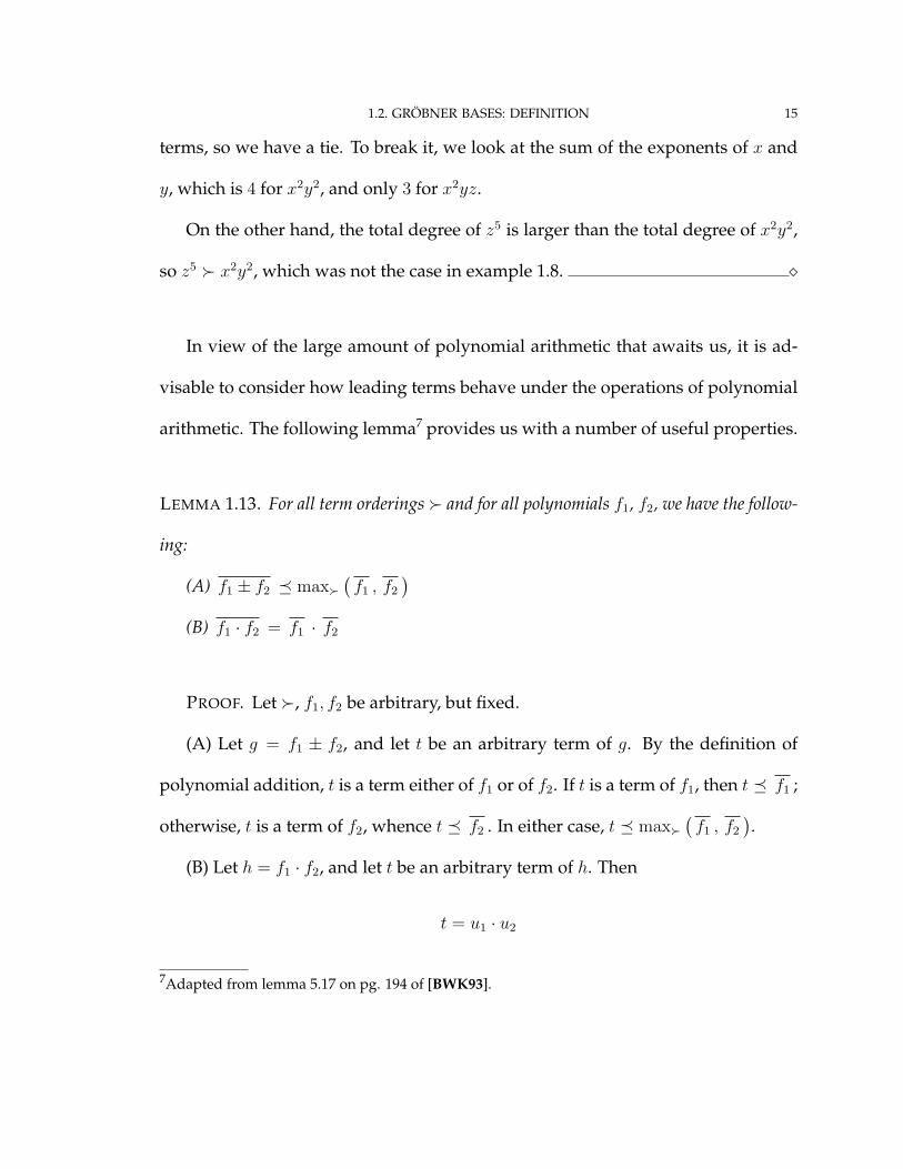
1.2. GRÖBNER BASES: DEFINITION 15
terms, so we have a tie. To break it, we look at the sum of the exponents of x and
y, which is 4 for x2y2, and only 3 for x2yz.
On the other hand, the total degree of z5 is larger than the total degree of x2y2,
so z5 � x2y2, which was not the case in example 1.8. �
In view of the large amount of polynomial arithmetic that awaits us, it is ad-
visable to consider how leading terms behave under the operations of polynomial
arithmetic. The following lemma7 provides us with a number of useful properties.
LEMMA 1.13. For all term orderings � and for all polynomials f1, f2, we have the follow-
ing:
(A) f1 ± f2 � max�(f1 , f2
)(B) f1 · f2 = f1 · f2
PROOF. Let �, f1, f2 be arbitrary, but fixed.
(A) Let g = f1 ± f2, and let t be an arbitrary term of g. By the definition of
polynomial addition, t is a term either of f1 or of f2. If t is a term of f1, then t � f1 ;
otherwise, t is a term of f2, whence t � f2 . In either case, t � max�(f1 , f2
).
(B) Let h = f1 · f2, and let t be an arbitrary term of h. Then
t = u1 · u2
7Adapted from lemma 5.17 on pg. 194 of [BWK93].

1.2. GRÖBNER BASES: DEFINITION 16
where u1 is a term of f1, and u2 is a term of f2. Clearly u1 � f1 and u2 � f2 . Thus
t = u1 · u2 � f1 · u2 � f1 · f2 �
COROLLARY 1.14. For all term orderings � and for all polynomials f1, f2, we have the
following:
(A) f1 ± f2 � max�
(f1 , f2
)(B) f1 · f2 = f1 · f2
(B) lc� (f1 · f2) = lc� (f1) · lc� (f2)
1.2.3. REDUCTION OF A POLYNOMIAL MODULO f1, . . . , fm. The essence of reduc-
tion is obtaining a remainder by division. This is comparable to Gaussian elimina-
tion in matrices, insofar as we reduce one row of a matrix by adding multiples of
other rows to it.
DEFINITION 1.15. Given polynomials p, f, f1, . . . , fm, r and a term ordering �, we
write:
• p −→f
r
if there exists a monomial q and a monomial d of p such that q ·
lm� (f) = d and r = p− qf
• p −→q·f
r
as an explicit synonym for the above
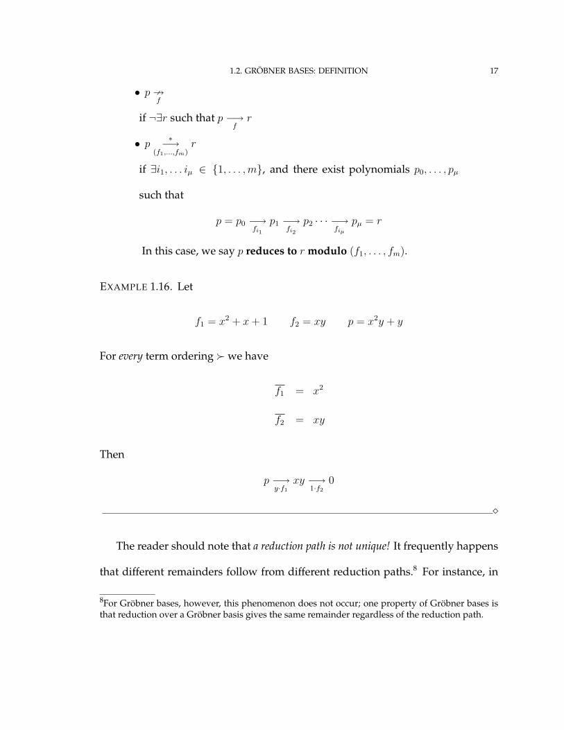
1.2. GRÖBNER BASES: DEFINITION 17
• p 9f
if ¬∃r such that p −→f
r
• p∗−→
(f1,...,fm)r
if ∃i1, . . . iµ ∈ {1, . . . ,m}, and there exist polynomials p0, . . . , pµ
such that
p = p0 −→fi1
p1 −→fi2
p2 · · · −→fiµ
pµ = r
In this case, we say p reduces to r modulo (f1, . . . , fm).
EXAMPLE 1.16. Let
f1 = x2 + x + 1 f2 = xy p = x2y + y
For every term ordering �we have
f1 = x2
f2 = xy
Then
p −→y·f1
xy −→1·f2
0
�
The reader should note that a reduction path is not unique! It frequently happens
that different remainders follow from different reduction paths.8 For instance, in
8For Gröbner bases, however, this phenomenon does not occur; one property of Gröbner bases isthat reduction over a Gröbner basis gives the same remainder regardless of the reduction path.

1.2. GRÖBNER BASES: DEFINITION 18
example 1.16, we could have reduced
p −→x·f2
y∗9
(f1,f2)
Hence
p∗−→
(f1,f2)0 and p
∗−→(f1,f2)
y
1.2.4. FORMAL DEFINITION OF A GRÖBNER BASIS. We introduced Gröbner bases
with an analogy from linear algebra; namely, comparing them to the “nice form”
provided by Gaussian elimination. In the case of linear polynomials, this “nice
form” is a basis of the vector space generated by f1, . . . , fm. We will define Gröbner
bases by drawing an analogy with a property of bases of vector spaces.
Recall from linear algebra that for polynomials f1, . . . , fm, if {b1, . . . , bM} is a
basis of the vector space
V = {c1f1 + · · ·+ cmfm : ck ∈ F}
then for all v ∈ V , Gaussian elimination of v over b1, . . . , bM compares to polyno-
mial reduction of v by b1, . . . , bM ; indeed
v = v0 −→(b1,...,bM )
v1 −→(b1,...,bM )
· · · −→(b1,...,bM )
vM = 0
In other words, v∗−→
(b1,...,bM )0. Note that the resulting quotients give co-ordinates of v
with respect to b1, . . . , bM . This follows from the fact that the bk generate the vector
space.

1.2. GRÖBNER BASES: DEFINITION 19
EXAMPLE 1.17. Let
f1 = x + y
f2 = y + 1
Note that x is a monomial of f1, but not of f2; hence the two polynomials are
linearly independent, thus a basis for
V = {c1f1 + c2f2 : c1, c2 ∈ Q}
Let g = 10f1 − 10f2. Clearly g ∈ V . Then
g = 10x− 10 −→10·f1
−10y − 10 −→−10·f2
0
Notice that the quotients give the co-ordinates of g with respect to f1, f2. �
Now define
I (f1, . . . , fm) = {h1f1 + · · ·+ hmfm : hk ∈ F[x1, . . . , xn]}
We define a Gröbner basis as if it gave a non-linear generalization of the above
property of the basis of a vector space.
DEFINITION 1.18. We say that f1, . . . , fm ∈ F[x1, . . . , xn] are a Gröbner basis with
respect to the term ordering � if for every p ∈ I we have p∗−→
(f1,··· ,fm)0.9
9This is not the only way to define a Gröbner basis. Our definition comes from [BWK93] (definition5.37 on page 207 and condition (v) of theorem 5.35 on page 206). The interested reader can findother definitions:
1.2. GRÖBNER BASES: DEFINITION 20
If f1, . . . , fm are a Gröbner basis, then we may write GB� (f1, . . . , fm) for short.
To familiarize ourselves with this definition, we reconsider the polynomials of
examples 1.1 and 1.2.
EXAMPLE 1.19. Let
f1 = 2x + 3y + 1
f2 = x + y
Notice that f1, f2 are derived from 1.1 on page 3.
To work in Gröbner bases, we need a term ordering, say �= lex (x, y). Thus
f1 = x f2 = x
We claim that f1, f2 are not a Gröbner basis with respect to �. Why not?
Let
p = 1 · f1 − 2 · f2
= (2x + 3y + 1)− 2 (x + y)
= y + 1
• [CLO98] (definition 3.1 on page 12), [Coh03] (definition 8.30 on page 324), andmore generally [Eis95] define a Gröbner basis so that for every p ∈ I, we havefi | g for some i = 1, . . . ,m;• [CLO97] (Definition 5 on page 74) and [vzGG99] (definition 21.25 on page 579)
use the definition that the ideal of the leading terms of f1, . . . , fm equals theideal of the leading terms of all p ∈ I.
Both these definitions also appear in [BWK93] (definition 5.37 on page 207 and condition (viii) oftheorem 5.35 on page 206). It should come as no surprise that these definitions are equivalent;proving this fact is the point of theorem 5.35 of [BWK93].

1.2. GRÖBNER BASES: DEFINITION 21
(Notice that p is the polynomial we obtained by Gaussian elimination in example
1.1.)
Certainly p ∈ I (f1, f2). However, neither f1 nor f2 divides any term of p.
Hence
p 9(f1,f2)
which implies that
p∗9
(f1,f2)0
Since f1, f2 do not satisfy definition 1.18, they are not a Gröbner basis. �
EXAMPLE 1.20. This time, let f1, f2 be as in example 1.2:
f1 = x2 + y2
f2 = xy
Again, let �= lex (x, y), so
f1 = x2 f2 = xy
We claim that f1, f2 are not a Gröbner basis. Let
p = y · f1 − x · f2
=(x2y + y3
)− x2y
= y3

1.3. GRÖBNER BASES: DECISION 22
(Notice that p is the polynomial f3 that we identified in example 1.2.)
Certainly p ∈ I (f1, f2). However, neither f1 nor f2 divides any term of p.
Hence
p 9(f1,f2)
which implies that
p∗9
(f1,f2)0
Since f1, f2 do not satisfy definition 1.18, they are not a Gröbner basis. �
At the end of example 1.2, we claimed that by appending f3, we did have the
“nice form.” In essence, we were claiming that f1, f2, f3 are a Gröbner basis with
respect to �. We would like to show this, but we cannot yet sit down and verify
that for all p ∈ I (f1, f2, f3), p∗−→
(f1,f2,f3)0.
How do we prove this claim?
1.3. GRÖBNER BASES: DECISION
Definition 1.18 does not suggest an algorithm that will decide whether the poly-
nomials f1, . . . , fm are a Gröbner basis. We cannot apply the definition directly,
since it is universally quantified over the p, and we would have to test infinitely
many p ∈ I (f1, . . . , fm).

1.3. GRÖBNER BASES: DECISION 23
In order to check whether some given polynomials are a Gröbner basis, we
need equivalent conditions that are not universally quantified over I. We present
these conditions as theorem 1.30 of section 1.3.3. Before we can present theorem
1.30, however, we have two more items of background material.10
1.3.1. S-POLYNOMIALS. For linear polynomials, we cancel the pivots by multiply-
ing appropriate scalar factors. For non-linear polynomials, we cancel the leading
terms by multiplying appropriate monomial factors. The construction that accom-
plishes this is the S-polynomial:
DEFINITION 1.21. For polynomials f1, f2 and for a term ordering �
S� (f1, f2) =lcm (lt� (f1) , lt� (f2))
lm� (f1)· f1 −
lcm (lt� (f1) , lt� (f2))
lm� (f2)· f2
We call S� (f1, f2) the S-polynomial of f1 and f2; the S stands for subtraction.11
When the term ordering � is understood from the context, we will write Sf1,f2 or
even S1,2.
10There is also the question of how to compute a Gröbner basis for f1, . . . , fm in the case wherethey are not a Gröbner basis themselves. There are several well-known algorithms for this: BrunoBuchberger’s algorithm of [Buc65] is the most famous, and more recently there are Faugère’s al-gorithms F4 [Fau99] and F5 [Fau02]. All these algorithms require a sub-algorithm that decideswhether a set of polynomials is a Gröbner basis; this is the focus of our particular research A dis-cussion of Gröbner basis computation lies beyond the scope of this thesis, and we refer the readerto the sources.11Buchberger refers to the S-polynomial as a subtraction polynomial in his thesis [Buc65], althoughCox, Little, and O’Shea refer to it as a syzygy polynomial in their text [CLO97]. The latter authorsare trying to place S-polynomials in this very important context of syzygies.
1.3. GRÖBNER BASES: DECISION 24
Note that Si,j = −Sj,i. As a result, we consider only the S-polynomials with
i < j.
The polynomials p of examples 1.19 on page 20 and 1.20 on page 21 were
formed by a construction very similar to that of S-polynomials. Compare their
results to examples 1.22 and 1.23.
EXAMPLE 1.22. Let
f1 = 2x + 3y + 1
f2 = x + y
We will use �= lex (x, y). Then
S1,2 =lcm (x, x)
2x· (2x + 3y + 1)− lcm (x, x)
x· (x + y)
=x
2x· (2x + 3y + 1)− x
x· (x + y)
=1
2· (2x + 3y + 1)− (x + y)
= x +3
2· y +
1
2− x− y
=1
2· y +
1
2
Notice that S1,2 is a constant multiple of p in example 1.19 on page 20, which, as
we noted, is the polynomial we found by Gaussian elimination in example 1.1 on
page 3. �
1.3. GRÖBNER BASES: DECISION 25
EXAMPLE 1.23. Let
f1 = x2 + y2
f2 = xy
Again, let �= lex (x, y). This gives us
f1 = x2
f2 = xy
Then
S1,2 =lcm (x2, xy)
x2·(x2 + y2
)− lcm (x2, xy)
xy· xy
=x2y
x2·(x2 + y2
)− x2y
xy· xy
= y ·(x2 + y2
)− x · xy
=(x2y + y3
)− x2y
= y3
Compare this to f3 and p in examples 1.2 on page 4 and 1.20 on page 21, respec-
tively. �
We leave it as an exercise for the reader to show that, for the polynomials given
in example 1.23,
S�lex(x,y)(f1, f2) = S�tdeg(x,y)
(f1, f2)

1.3. GRÖBNER BASES: DECISION 26
However, the S-polynomial can also change if we change the term ordering, as
illustrated by example 1.24.
EXAMPLE 1.24. Let f1, f2 be as in example 1.23. This time, let �= lex (y, x). Now
we have f1 = y2. Then
S1,2 =lcm (y2, xy)
y2·(x2 + y2
)− lcm (y2, xy)
xy· xy
=xy2
y2·(x2 + y2
)− xy2
xy· xy
= x ·(x2 + y2
)− y · xy
=(x3 + xy2
)− xy2
= x3
�
The following lemma formalizes the observation that S-polynomials eliminate
leading terms, and it provides an unreachable “upper bound” for the leading terms
of S-polynomials.
LEMMA 1.25. For all fi, fj ∈ F[x1, . . . , xn]
Si,j ≺ lcm(fi , fj
)PROOF. Let fi, fj ∈ F[x1, . . . , xn] be arbitrary, but fixed. Recall that
Si,j =lcm
(fi , fj
)fi
· fi −lcm
(fi , fj
)fi
· fi

1.3. GRÖBNER BASES: DECISION 27
Write fi = fi + Ri and fj = fj + Rj . Then
Si,j =lcm
(fi , fj
)fi
·(
fi + Ri
)−
lcm(fi , fj
)fi
·(
fj + Rj
)=lcm
(fi , fj
)+
lcm(fi , fj
)fi
·Ri − lcm(fi , fj
)−
lcm(fi , fj
)fi
·Rj
=lcm
(fi , fj
)fi
·Ri −lcm
(fi , fj
)fj
·Rj
Clearly,
Si,j = max�
(lcm
(fi , fj
)fi
·Ri ,lcm
(fi , fj
)fj
·Rj
)Observe that
lcm(fi , fj
)fi
·Ri =lcm
(fi , fj
)fi
· Ri
≺lcm
(fi , fj
)fi
· fi
= lcm(fi , fj
)Similarly,
lcm(fi , fj
)fi
·Ri ≺ lcm(fi , fj
)Thus
Si,j ≺ lcm(fi , fj
)�
1.3.2. REPRESENTATION OF AN S-POLYNOMIAL MODULO f1, . . . , fm. Suppose we
perform Gaussian elimination on the linear polynomials f1, . . . , fm and obtain the
1.3. GRÖBNER BASES: DECISION 28
linear basis b1, . . . , bM . We alluded in example 1.17 on page 18 to the fact that if
p = c1f1 + · · ·+ cmfm
where the ck are scalars in the base field, then we can represent p in terms of
b1, . . . , bM by its co-ordinates.
We extend this idea to the concept of the representation of an S-polynomial
modulo f1, . . . , fm:12
DEFINITION 1.26. We say that h1, . . . , hm give a representation of Si,j modulo
f1, . . . , fm if
Si,j = h1f1 + · · ·+ hmfm
and for every k = 1, . . . ,m hk 6= 0 implies
hk · fk ≺ lcm(fi , fj
)If ∃h1, . . . , hm such that h1, . . . , hm give a representation of Si,j modulo f1, . . . , fm,
we say that Si,j has a representation modulo f1, . . . , fm. We often omit the modu-
lus if it is obvious from context.
With linear polynomials, we can find a representation for a polynomial p by
performing row-reduction operations on p using the basis b1, . . . , bM . It turns out
12We could define this more generally; see the standard representation of a polynomial on page 218of [BWK93]. For our purposes, the notion of an S-polynomial representation (a special case of thet-representation on page 219 of [BWK93]) will suffice.

1.3. GRÖBNER BASES: DECISION 29
that we can do something similar in the non-linear case using reduction and repre-
sentation. If we collect the monomial quotients of a reduction path, we can obtain
sample hk by adding the all monomial quotients for fk. We illustrate this in exam-
ple 1.27.
EXAMPLE 1.27. Let
f1 = x2 + x + 1 f2 = y − 1
Let � be any term ordering. Then
f1 = x2 f2 = y
We have
S1,2 =lcm (x2, y)
x2·(x2 + x + 1
)− lcm (x2, y)
y· (y − 1)
=y ·(x2 + x + 1
)− x2 · (y − 1)
=x2 + xy + y
Then
S1,2 −→1·f1
xy + y − x− 1 −→x·f2
y − 1 −→1·f2
0
Collecting and negating the monomials of the reduction path, we see that
S1,2 = h1f1 + h2f2
where
h1 = 1 h2 = x + 1

1.3. GRÖBNER BASES: DECISION 30
We have
h1 · f1 = 1 · x2 ≺ x2y = lcm(f1 , f2
)h2 · f2 = x · y ≺ x2y = lcm
(f1 , f2
)So h1 and h2 give us a representation of S1,2. �
Generalizing the above, we have the following lemma:
LEMMA 1.28. Let f1, . . . , fm be polynomials. For all 1 ≤ i < j ≤ m we have (A)⇒(B)
where
(A) Si,j∗−→
(f1,··· ,fm)0
(B) Si,j has a representation modulo f1, . . . , fm
PROOF. Let i 6= j be arbitrary, but fixed.
We want to show (A)⇒(B), so assume (A).
Then
Si,j∗−→
(f1,...,fm)0
Write out an explicit reduction path
(1.1) Si,j = p0 −→q1·fi1
p1 −→q2·fi2
· · · −→qr·fir
pr = 0
Notice that by the definition of reduction and lemma 1.25 on page 26, we have
for all ` = 1, . . . , r
q` · fi` � p`−1 � · · · � p0 = Si,j ≺ lcm(fi , fj
)
1.3. GRÖBNER BASES: DECISION 31
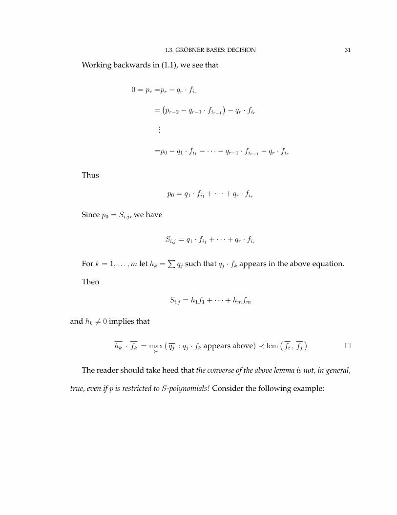
Working backwards in (1.1), we see that
0 = pr =pr − qr · fir
=(pr−2 − qr−1 · fir−1
)− qr · fir
...
=p0 − q1 · fi1 − · · · − qr−1 · fir−1 − qr · fir
Thus
p0 = q1 · fi1 + · · ·+ qr · fir
Since p0 = Si,j , we have
Si,j = q1 · fi1 + · · ·+ qr · fir
For k = 1, . . . ,m let hk =∑
qj such that qj · fk appears in the above equation.
Then
Si,j = h1f1 + · · ·+ hmfm
and hk 6= 0 implies that
hk · fk = max�
( qj : qj · fk appears above) ≺ lcm(fi , fj
)�
The reader should take heed that the converse of the above lemma is not, in general,
true, even if p is restricted to S-polynomials! Consider the following example:
1.3. GRÖBNER BASES: DECISION 32
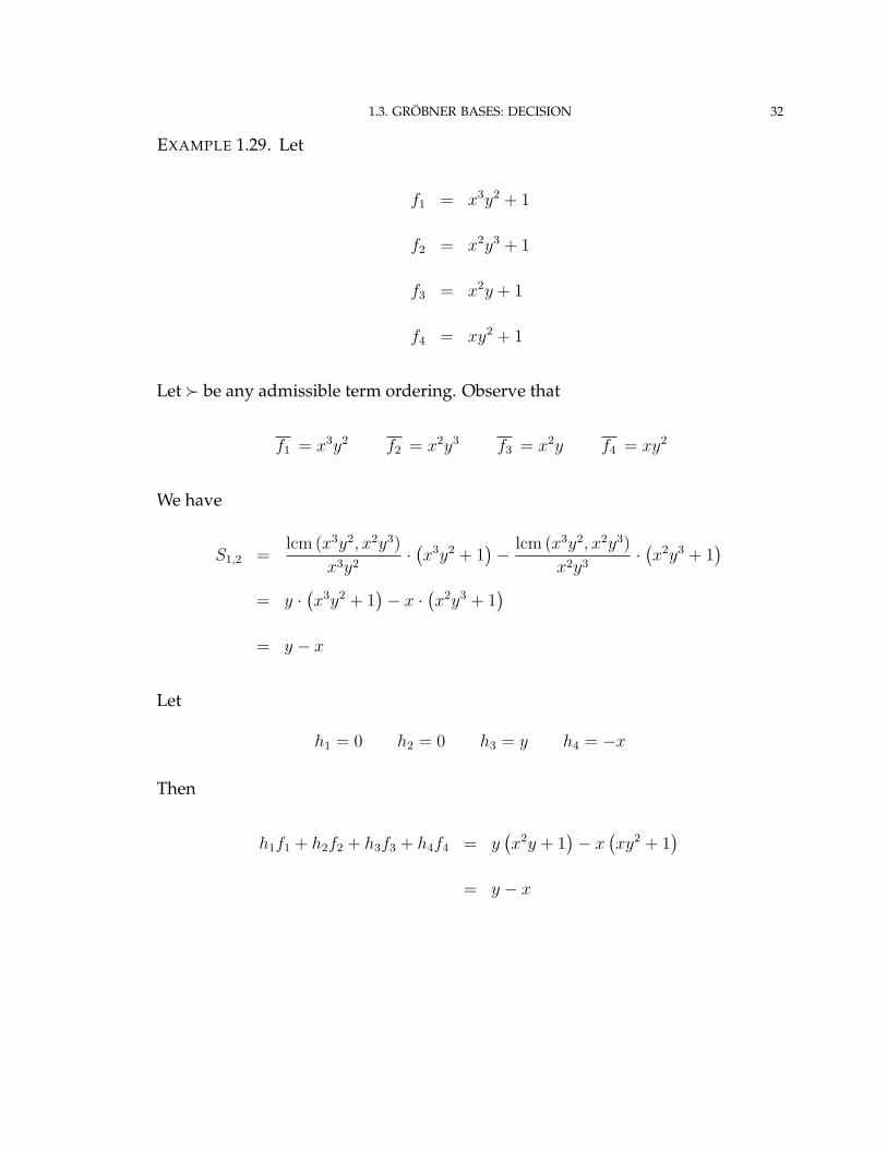
EXAMPLE 1.29. Let
f1 = x3y2 + 1
f2 = x2y3 + 1
f3 = x2y + 1
f4 = xy2 + 1
Let � be any admissible term ordering. Observe that
f1 = x3y2 f2 = x2y3 f3 = x2y f4 = xy2
We have
S1,2 =lcm (x3y2, x2y3)
x3y2·(x3y2 + 1
)− lcm (x3y2, x2y3)
x2y3·(x2y3 + 1
)= y ·
(x3y2 + 1
)− x ·
(x2y3 + 1
)= y − x
Let
h1 = 0 h2 = 0 h3 = y h4 = −x
Then
h1f1 + h2f2 + h3f3 + h4f4 = y(x2y + 1
)− x
(xy2 + 1
)= y − x
1.3. GRÖBNER BASES: DECISION 33
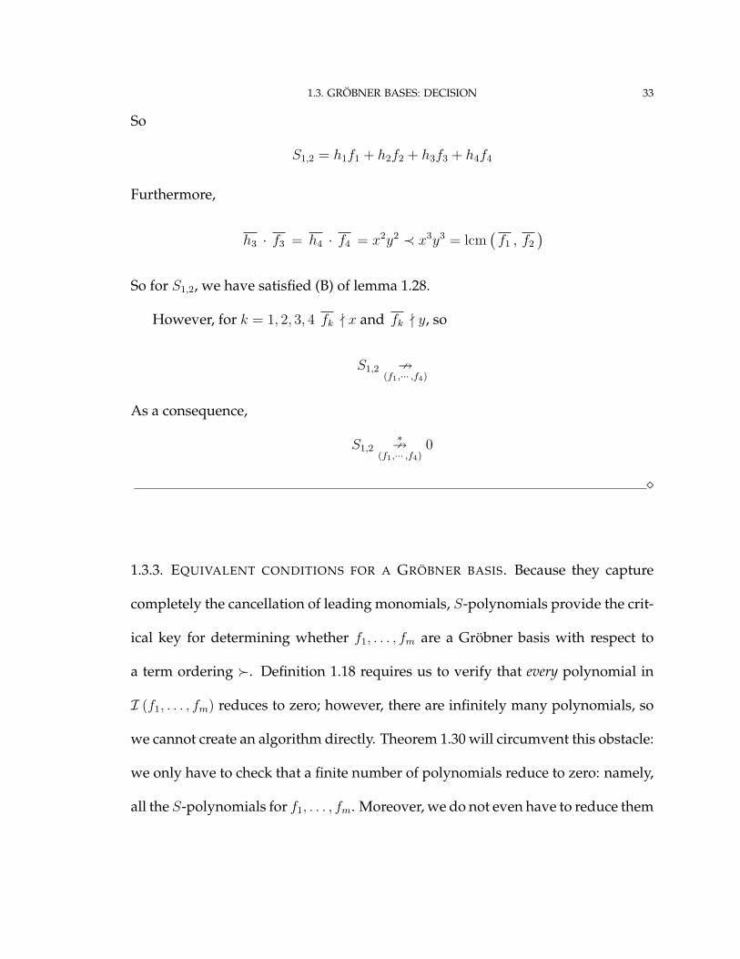
So
S1,2 = h1f1 + h2f2 + h3f3 + h4f4
Furthermore,
h3 · f3 = h4 · f4 = x2y2 ≺ x3y3 = lcm(f1 , f2
)So for S1,2, we have satisfied (B) of lemma 1.28.
However, for k = 1, 2, 3, 4 fk - x and fk - y, so
S1,2 9(f1,··· ,f4)
As a consequence,
S1,2∗9
(f1,··· ,f4)0
�
1.3.3. EQUIVALENT CONDITIONS FOR A GRÖBNER BASIS. Because they capture
completely the cancellation of leading monomials, S-polynomials provide the crit-
ical key for determining whether f1, . . . , fm are a Gröbner basis with respect to
a term ordering �. Definition 1.18 requires us to verify that every polynomial in
I (f1, . . . , fm) reduces to zero; however, there are infinitely many polynomials, so
we cannot create an algorithm directly. Theorem 1.30 will circumvent this obstacle:
we only have to check that a finite number of polynomials reduce to zero: namely,
all the S-polynomials for f1, . . . , fm. Moreover, we do not even have to reduce them
1.3. GRÖBNER BASES: DECISION 34
to zero; the theorem shows that having representations for all the S-polynomials
is also equivalent.
THEOREM 1.30. For all f1, . . . , fm and for all �, the following are equivalent.
(A) f1, . . . , fm are a Gröbner basis with respect to �.
(B) for all 1 ≤ i < j ≤ m, Si,j∗−→
(f1,...,fm)0.
(C) for all 1 ≤ i < j ≤ m, Si,j has a representation modulo f1, . . . , fm.
The proof is rather long, so we present it at the end of the section. We precede
the proof with an algorithm that follows naturally from clause (B), and with some
examples.
First, a caution on what the theorem does not say. The positions of the quanti-
fiers are essential; it is not the case that
∀1 ≤ i < j ≤ m
[Si,j
∗−→(f1,...,fm)
0 ⇔ Si,j has a representation modulo f1, . . . , fm
](Recall example 1.29 on page 31.)
AN ALGORITHM FOR THEOREM 1.30. Clause (B) of theorem 1.30 lends itself nat-
urally to an algorithm to decide whether a system of polynomials are a Gröbner
basis with respect to a given term ordering, and we present this as algorithm 1.1.
The algorithm is a straightforward implementation of theorem 1.30, so it clearly
terminates correctly.

1.3. GRÖBNER BASES: DECISION 35
Algorithm 1.1 Is_GBInputs: �, f1, . . . , fm
Output: YESif f1, . . . , fm are a Gröbner basis with respect to �; NOotherwise.
B ← {(i, j) : 1 ≤ i < j ≤ m}
For (i, j) ∈ B Do
If Si,j∗9
(f1,...,fm)0 Then
Return FALSE
Return TRUE
EXAMPLES OF THEOREM 1.30. Now for some examples. The first ones are those
that we could not verify previously. The first example is the linear system derived
from example 1.1 on page 3.
EXAMPLE 1.31. Recall from example 1.22 on page 24
f2 = x + y
Let
f3 = y + 1
Notice f3 = S1,2 (where f1 = 2x + 3y + 1 as in example 1.22).
We claim that f2, f3 are a Gröbner basis with respect to �. Observe that
S2,3 =lcm (x, y)
x· (x + y)− lcm (x, y)
y· (y + 1)
=(xy + y2
)− (xy + x)
=y2 − x

1.3. GRÖBNER BASES: DECISION 36
Then
S2,3 −→f2
y2 + y −→−2y·f3
0
By theorem 1.30, f2, f3 are a Gröbner basis with respect to �. �
We leave it as an exercise to the reader to show that f1, f2, f3 from example 1.22
on page 24 are also a Gröbner basis with respect to �. However, it is not necessary
to include f1 in the Gröbner basis, since f1 ∈ I (f2, f3):
f1 = 2f2 + f3
Recalling example 1.2 on page 4, we now show that the non-linear f1, f2, f3 do
have the “nice form”, and that we cannot drop any one of the three.
EXAMPLE 1.32. Let �= lex (x, y). Recall from examples 1.2 on page 4 and 1.23 on
page 25
f1 =x2 + y2
f2 =xy
f3 =y3
According to theorem 1.30, we need to verify that S1,2, S1,3, S2,3 all reduce to zero
over f1, f2, f3.
We saw in example 1.23 on page 25 that S1,2 = f3, so
S1,2∗−→
(f1,f2,f3)0

1.3. GRÖBNER BASES: DECISION 37
We also have
S1,3 =lcm (x2, y3)
x2·(x2 + y2
)− lcm (x2, y3)
y3· y3
=(x2y3 + y5
)− x2y3
=y5
Here
S1,3 −→y2·f3
0
so
S1,3∗−→
(f1,f2,f3)0
Finally, S2,3 = 0 so S2,3∗−→
(f1,f2,f3)0.
Since all of S1,2, S1,3, S2,3 reduce to zero over f1, f2, f3, theorem 1.30 informs us
that f1, f2, f3 are a Gröbner basis with respect to �. �
The reader should note that the steps we followed in example 1.32 are not only
the steps necessary to verify that clause (B) of theorem 1.30 holds, but they are also
the precise steps that we followed in example 1.2 on page 4, a generalization of
Gaussian elimination.
The choice of term ordering can affect whether a set of polynomials is a Gröb-
ner basis. This should make sense, since we have seen already that changing the
term ordering can change the leading terms, the S-polynomials, and the possible
reduction paths – in other words, everything can hinge on the term ordering.

1.3. GRÖBNER BASES: DECISION 38
Example 1.33 illustrates this fact. We reconsider the polynomials of example
1.32 using a different term ordering.
EXAMPLE 1.33. Let f1, f2, f3 be as in example 1.2; that is,
f1 =x2 + y2
f2 =xy
f3 =y3
We claim that f1, f2, f3 are not a Gröbner basis with respect to �= lex (y, x).
Notice first that one of the leading terms has changed! We now have
f1 = y2 f2 = xy f4 = y3
Then
S1,2 =lcm (y2, xy)
y2·(x2 + y2
)− lcm (y2, xy)
xy· xy
=(x3 + xy2
)− xy2
=x3
We cannot carry out a single reduction! Hence
S1,2∗9
(f1,f2,f3)0
We conclude that f1, f2, f3 are not a Gröbner basis with respect to �. �
1.3. GRÖBNER BASES: DECISION 39
PROOF OF THEOREM 1.30. We conclude section 1.3.3 with a proof of theorem 1.30.
First, we restate the theorem:
THEOREM. For all f1, . . . , fm and for all �, the following are equivalent.
(A) f1, . . . , fm are a Gröbner basis with respect to �.
(B) for all 1 ≤ i < j ≤ m, Si,j∗−→
(f1,...,fm)0.
(C) for all 1 ≤ i < j ≤ m, Si,j has a representation modulo f1, . . . , fm.
The proof has three major sections:
• (A)⇒(B) (short)
• (B)⇒(C) (very short)
• (C)⇒(A) (long: pages 40 – 48)
PROOF. (Of theorem 1.30)
Let f1, . . . , fm, and � be arbitrary, but fixed.
(A)⇒(B): Assume (A). So f1, . . . , fm are a Gröbner basis with respect to �.
Let i < j satisfy (B).
Recall that
Si,j =lcm
(fi , fj
)fi
· fi −lcm
(fi , fj
)fj
· fj
We have
Si,j = h1f1 + · · ·+ hmfm

1.3. GRÖBNER BASES: DECISION 40
where
hi =lcm
(fi , fj
)fi
· fi
hj =lcm
(fi , fj
)fj
· fj
hk =0 ∀k 6= i, j
Then
Si,j ∈ I (f1, . . . , fm)
Recall that f1, . . . , fm are a Gröbner basis. Hence, for every p ∈ I (f1, . . . , fm),
p∗−→
(f1,...,fm)0. In particular, Si,j
∗−→(f1,...,fm)
0.
But i, j were arbitrary. Hence (B).
(B)⇒(C): This is a consequence of lemma 1.28 on page 30.
(C)⇒(A): Assume (C).13
Abbreviate I (f1, . . . , fm) as I. We have to show that p∗−→
(f1,...,fm)0 for every p ∈ I.
We proceed in three steps, each of which is a claim. Claim 1 is by far the longest.
Claim 1. We claim that for every nonzero p ∈ I ∃h1, . . . , hm such that
(1.2) p = h1f1 + · · ·+ hmfm
and ∀k = 1, . . . ,m hk · fk � p .
Let p ∈ I be arbitrary, but fixed.
13The following is derived from the proofs of theorem 5.64, lemma 5.61, and theorem 5.35 of[BWK93].
1.3. GRÖBNER BASES: DECISION 41
Let
R = {(h1, . . . , hm) : p = h1f1 + · · ·+ hmf}
and
S ={max
(h1 · f1 , . . . , hm · fm
): (h1, . . . , hm) ∈ R
}Since S ⊂ T (x1, . . . , xn), S has a least element with respect to �; call it s.
Clearly s � p : we have s � p only if two terms on the right-hand side of (1.2)
cancel. We claim that by choosing h1, . . . , hm so that s is minimal, we have p = s.
Note that this would imply claim 1.
By way of contradiction, assume that s � p . Then the terms on the right-hand
side of (1.2) that contain s must cancel.
Let n be the number of leading terms of the hkfk such that hk · fk = s. Note
that n > 1.
We claim that if for some M ≤ n
s = hk1 · fk1 = · · · = hkM· fkM
and
hk1 · fk1 + · · ·+ hkM· fkM
= 0
then we can rewrite
(1.3) hk1fk1 + · · ·+ hkMfkM

1.3. GRÖBNER BASES: DECISION 42
such that
s′ = max�
{hk`· fk`
: ` = 1, . . . ,M}≺ s
We proceed by induction on M .
Inductive base: Assume that M = 2. Without loss of generality,
h1 · f1 = h2 · f2 = s
and
h1 · f1 + h2 · f2 = 0
Thus
lcm(f1 , f2
)| s
Let u be such that
u · lcm(f1 , f2
)= s
Let ak = lc� (hk) and bk = lc� (fk); then
a1b1 = −a2b2
Put
c = a1b1 = −a2b2
Then
h1 · f1 + h2 · f2 =a1 h1 · f1 + a2 h2 · f2
=a1 h1 · f1 ·f1
f1
+ a2 h2 · f2 ·f2
f2
1.3. GRÖBNER BASES: DECISION 43
=a1 h1 · b1 f1 ·f1
f1
+ a2 h2 · b2 f2 ·f2
f2
=c · h1 · f1 ·f1
f1
− c · h2 · f2 ·f2
f2
=cs · f1
f1
− cs · f2
f2
=cs ·(
f1
f1
− f2
f2
)=c · u · lcm
(f1 , f2
)·(
f1
f1
− f2
f2
)=cu ·
(lcm
(f1 , f2
)f1
· f1 −lcm
(f1 , f2
)f2
· f2
)
=cu · S1,2
We had assumed (C), so there exist H1, . . . , Hm such that
(1.4) S1,2 = H1f1 + · · ·+ Hmfm
and for k = 1, . . . ,m Hk 6= 0 implies
Hk · fk ≺ lcm(f1 , f2
)Thus
(1.5) u · Hk · fk ≺ u · lcm(f1 , f2
)= s
Recalling (1.2), we have
p =h1f1 + h2f2 + h3f3 + · · ·+ hmfm
=[h1 · f1 + h2 · f2
]+[(
h1 − h1
)· f1 +
(h2 − h2
)· f2 + h3f3 + · · ·+ hmfm
]

1.3. GRÖBNER BASES: DECISION 44
=cu · S1,2 +[(
h1 − h1
)· f1 +
(h2 − h2
)· f2 + h3f3 + · · ·+ hmfm
]=cu · (H1f1 + · · ·+ Hmfm)
= +[(
h1 − h1
)· f1 +
(h2 − h2
)· f2 + h3f3 + · · ·+ hmfm
]Collecting on f1, . . . , fm we have
p =(cu ·H1 + h1 − h1
)· f1 +
(cu ·H2 + h2 − h2
)· f2
+ (cu ·H3 + h3) f3 + · · ·+ (cu ·Hm + hm) fm(1.6)
Note that we have removed h1 · f1 and h2 · f2 from this last equation, so we
removed the two instances where s appeared in (1.2).
Recall from (1.5) that u · Hk · fk ≺ s for k = 1, . . . ,m.
Since M = 2, we know that hk · fk ≺ s for k = 3, . . . ,m.
Let
s′ = max{
u ·H1 + h1 − h1 · f1 ,
u ·H2 + h2 − h2 · f2 ,
u ·H3 + h3 · f3 ,
. . . ,
u ·Hm + hm · fm
}

1.3. GRÖBNER BASES: DECISION 45
Since s′ is from the leading terms of (1.6), we see that s′ 6= s. No term larger than s
was added during the construction of (1.6), and s was maximal among the hk · fk ,
so s′ ≺ s.
Inductive step: Assume that M > 2, and if
• hk1 · fk1 + hk2 · fk2 = 0
• . . .
• hk1 · fk1 + · · ·+ hkM−1· fkM−1
= 0
then we can rewrite (1.3) such that s′ = max�{
hk · fk
}≺ s. Since M > 2,
hk1 · fk1 + · · ·+ hkM· fkM
= 0
Without loss of generality, we may assume that
h1 · f1 = · · · = hM · fM = s
so that
h1 · f1 + · · ·+ hM · fM = 0
Write
lc� (hk) = ak lc� (fk) = bk
Certainly
(1.7) p = h1f1 −a1b1
a2b2
· h2 · f2 +
(h2 +
a1b1
a2b2
· h2
)· f2 + h3f3 · · ·+ hmfm

1.3. GRÖBNER BASES: DECISION 46
Notice that the leading monomials of the first two summands are constant multi-
ples of s, and they cancel:
h1 · f1 −a1b1
a2b2
· h2 · f2 = h1 · f1 − a1b1 · h2 · f2
= a1b1s− a1b1s
= 0
The inductive hypothesis applies here, so that we can rewrite
h1f1 −a1b1
a2b2
· h2 · f2 = H1f1 +H2f2
with
s′ = max�
{H1 · f1 , H2 · f2
}≺ s
In the last m − 1 summands of (1.7), s must cancel. There are exactly M − 2
occurrences of s in h3 · f3 , . . . , hM · fM . Further, there is only one occurrence of s
in
h2 +a1b1
a2b2
· h2 · f2
So s appears exactly M −1 times in the last m−1 summands of (1.7); the inductive
hypothesis applies to these summands as well.
Regardless of the value of M , we have found an expression
p = H1 · f1 + · · ·+Hm · fm

1.3. GRÖBNER BASES: DECISION 47
where
s′ = max�
{Hk · fk : k = 1, . . . ,m
}≺ s
This contradicts the choice of s, so our assumption that s � p was wrong. We have
shown that (C) implies that
∀p ∈ I ∃h1, . . . , hm ∈ F[x1, . . . , xn] p = h1f1 + · · ·+ hmfm ∧ hk · fk � p
Claim 2. For every nonzero p ∈ I, fk | p for some k = 1, . . . m.
Let p ∈ I be arbitrary, but fixed.
From claim 1, ∃h1, . . . , hm such that p = h1f1 + · · ·hmfm and hk · fk � p for
k = 1, . . . ,m.
Certainly hk · fk = p for some k = 1, . . . ,m (otherwise the equations cannot
be equal).
For this k, we have fk | p .
Claim 3. We claim that ∀p ∈ I p∗−→
(f1,...,fm)0.
Let p ∈ I be arbitrary, but fixed. Let r be such that
p∗−→
(f1,...,fm)r 9
(f1,...,fm)
If r 6= 0, then from claim 2 we know fk | r for some k = 1, . . . ,m.
This contradicts r 9(f1,...,fm)
.
Thus r = 0 and
p∗−→
(f1,...,fm)0 �

1.4. SOME PROPERTIES OF REPRESENTATIONS OF S-POLYNOMIALS 48
1.4. SOME PROPERTIES OF REPRESENTATIONS OF S-POLYNOMIALS
Although the climax of this chapter is theorem 1.30, we will need some ad-
ditional tools in subsequent chapters. These tools describe elementary properties
of representations of S-polynomials, and they pop up in multiple chapters, so we
present them here.
We begin by defining notation for the “magic monomials” used to create S-
polynomials.14
DEFINITION 1.34. For all polynomials fi, fj and term orderings �, we write
σij =lcm
(fi , fj
)fi
σji =lcm
(fi , fj
)fj
This gives us an abbreviated notation for S-polynomials:
Si,j = σij · fi − σji · fj
This abbreviated notation for S-polynomials is not the reason we introduce the
σ-notation. These “magic monomials” will prove very important to subsequent
results.
What relationship exists between σij and σji, the two monomials used to create
Si,j? It turns out that the two are relatively prime on their indeterminates.
14We are adapting this extremely useful notation from [Hon98].
1.4. SOME PROPERTIES OF REPRESENTATIONS OF S-POLYNOMIALS 49
LEMMA 1.35. For all i 6= j, gcd ( σij , σji ) = 1.
PROOF. Let i 6= j. Assume x | σij .
We have
degx σij = degx
(lcm
(fi , fj
)fi
)
= degx lcm(fi , fj
)− degx fi
= max(degx fi , degx fj
)− degx fi
= max(0, degx fj − degx fi
)Since x | σij , degx σij > 0. Thus
degx fj > degx fi
Now consider
degx σji = degx
(lcm
(fi , fj
)fj
)
= degx lcm(fi , fj
)− degx fj
= max(degx fi , degx fj
)− degx fj
= degx fj − degx fj
=0
Since x was an arbitrary indeterminate such that x | σij , we know that degx σji =
0 for any indeterminate x where x | σij .

1.4. SOME PROPERTIES OF REPRESENTATIONS OF S-POLYNOMIALS 50
A symmetric argument shows that degx σij = 0 for any indeterminate x where
x | σji.
Hence gcd ( σij , σji ) = 1 as claimed. �
The next result is a useful consequence of lemma 1.25 on page 26.
LEMMA 1.36. For all i 6= j (A)⇒(B) where
(A) h1, . . . , hm give a representation of Si,j modulo f1, . . . , fm
(B) (σij ± hi) = σij and (σji ± hj) = σji
PROOF. Let i 6= j be arbitrary, but fixed.
Assume (A).
The statement of (B) is equivalent to σij � hi and σji � hj .
By way of contradiction, assume
σij � hi
Using corollary 1.14 on page 16,
lcm(fi , fj
)fi
� hi
lcm(fi , fj
)� hi · fi
Recall (A). Since h1, . . . , hm give a representation of Si,j , we know
hi · fi ≺ lcm(fi , fj
)We have a contradiction.
1.4. SOME PROPERTIES OF REPRESENTATIONS OF S-POLYNOMIALS 51
Hence σij � hi . That σji � hj is proved similarly. �
We will see in later chapters that it is useful to remove a common divisor from
the polynomials to study the representations of their S-polynomials. That is, sup-
pose c1, . . . , cm, g are polynomials such that fk = ckg. We would like to know how
to “descend” from a representation of Sfi,fjto a representation of Sci,cj
and how
to ascend again. What relationship, if any, exists between a representation of the
S-polynomial of ci, cj and the S-polynomial of fi, fj? Lemma 1.37 provides the
answer.
LEMMA 1.37. For all f1, . . . , fm where fk = ckg for some c1, . . . , cm, g, the following are
equivalent:
(A) h1, . . . , hm give a representation of Sfi,fjmodulo f1, . . . , fm
(B)H1, . . . ,Hm give a representation of Sci,cjmodulo c1, . . . , cm, whereHk = lc� (g) ·
hk
PROOF. Let � and f1, . . . , fm be arbitrary, but fixed. Assume ∃c1, . . . , cm, g such
that fk = ckg. Let i 6= j be arbitrary, but fixed, and let h1, . . . , h3 be arbitrary, but
fixed.
Then
Sfi,fj=h1f1 + · · ·+ hmfm
m

1.4. SOME PROPERTIES OF REPRESENTATIONS OF S-POLYNOMIALS 52
lcm(fi , fj
)fi
· fi −lcm
(fi , fj
)fj
· fj =h1f1 + · · ·+ hmfm
m
g ·(
lcm ( gci , gcj )
cig· ci −
lcm ( gci , gcj )
cjgcj
)=g · (h1c1 + · · ·+ hmcm)
m
g · lcm ( ci , cj )
g · ci
· ci −g · lcm ( ci , cj )
g · cj
cj =h1c1 + · · ·+ hmcm
m
1
lc� (g)·(
lcm ( ci , cj )
ci
· ci −lcm ( ci , cj )
cj
cj
)=h1c1 + · · ·+ hmcm
m
Sci,cj=H1c1 + · · ·+Hmcm
Moreover, for any k, if hk 6= 0 then
fk · hk ≺lcm(fi , fj
)m
ckg · hk ≺lcm ( cig , cjg )
m
g · ck · hk ≺ g · lcm ( ci , cj )
m
ck · hk ≺lcm ( ci , cj )
1.4. SOME PROPERTIES OF REPRESENTATIONS OF S-POLYNOMIALS 53
SinceHk is a constant multiple of hk, hk = Hk . Thus
ck · Hk ≺ lcm ( ci , cj )
From the preceding, we have the equivalence
Sfi,fj= h1f1 + · · ·+ hmfm
m
Sci,cj=H1c1 + · · ·+Hmcm
and for each k = 1, 2, 3 we have the equivalence
fkhk ≺lcm(fi , fj
)m
ckHk ≺lcm ( ci , cj )
The statement of the lemma follows from these two equivalences. �

Chapter 2
Skipping S-polynomial reductions
2.1. A BOTTLENECK
The most time-consuming step in algorithm 1.1 on page 35 is the reduction of
S-polynomials. Reduction can introduce growth in two ways: the storage size of
the coefficients, and the number of monomials. This phenomenon, appropriately
called “blowup”, has proven a challenge for many applications of Gröbner bases.1
Examining the algorithm, we see that for a set of M polynomials, there are
M (M − 1) S-polynomials to check. If we know a priori that some S-polynomials
reduce to zero, then we can skip their reduction. For example:
LEMMA 2.1. If fi and fj are monomials, then Si,j∗−→
(fi,fj)0.
1I can illustrate the bad reputation this phenomenon has given Gröbner bases using the followinganecdote: during a conversation, a specialist in algebraic geometry told me that another algebraicgeometer had advised him to steer away from Gröbner bases since, in the latter’s opinion, they areunusable for systems of more than 5 or 6 polynomials in 5 or 6 variables.
54

2.2. SKIPPING S-POLYNOMIAL REDUCTIONS 55
PROOF. Regardless of the term ordering, we have
fi =fi
fj =fj
Thus
Si,j =lcm
(fi , fj
)fi
· fi −lcm
(fi , fj
)fj
· fj
= lcm(fi , fj
)− lcm
(fi , fj
)= 0
So we have trivially
Si,j∗−→
(fi,fj)0 �
2.2. SKIPPING S-POLYNOMIAL REDUCTIONS
We now formalize the notion of skipping an S-polynomial reduction.
DEFINITION 2.2. Suppose we are given f1, . . . , fm and a term ordering. We say
that condition C allows us to skip the reduction of Si,j modulo f1, . . . , fm (written
Si,j 0) if C implies that ∃P such that
(A) P ⊂ {(k, `) : 1 ≤ k < ` ≤ m} and (i, j) 6∈ P
(B) If Sk,`∗−→
(f1,...,fm)0 for every (k, `) ∈ P , then GB� (f1, . . . , fm).
In other words, algorithm Is_GB ( 1.1 on page 35) does not need to reduce Si,j
to decide whether f1, . . . , fm are a Gröbner basis.
2.2. SKIPPING S-POLYNOMIAL REDUCTIONS 56
Certainly, if we knew a priori that Si,j reduces to zero, then we could skip its
reduction, so this definition makes sense.
On the other hand, what if all we knew was that Si,j has a representation?
Algorithm Is_GB ( 1.1 on page 35) checks whether every S-polynomial reduces to
zero, and definition 2.2 says nothing about representations of S-polynomials, and
we know that representation does not necessarily imply reduction to zero.
This is not such an obstacle as it may first seem. It turns out that having a
representation is equivalent to being able to skip an S-polynomial reduction:
LEMMA 2.3. (A) and (B) are equivalent, where
(A) Si,j has a representation.
(B) Si,j 0.
PROOF. Let f1, . . . , fm and � be arbitrary, but fixed.
(A)⇒(B): Assume that Si,j has a representation. Let P = {(k, `) : (k, `) 6= (i, j)}.
Assume that Sk,` reduces to zero for every (k, `) ∈ P ; applying lemma 1.28, every
S-polynomial in P has a representation. We know that Si,j has a representation;
thus every S-polynomial has a representation, so f1, . . . , fm are a Gröbner basis.
Thus Si,j 0.
(A)⇐(B): We proceed by showing the contrapositive: assume that Si,j does not
have a representation. By theorem 1.30 on page 34, f1, . . . , fm cannot be a Gröbner
2.2. SKIPPING S-POLYNOMIAL REDUCTIONS 57
basis regardless of the choice ofP (keeping in mind that (i, j) 6∈ P). Since f1, . . . , fm
are not a Gröbner basis for any value of P , we cannot skip Si,j . �
This result gives us a way to use representation to skip an S-polynomial re-
duction. In fact, we will never prove directly in this text that if some condition
C is true, then Si,j reduces to zero. Rather, we will prove that if some condition
C is true, then Si,j has a representation. Why? Besides an aesthetic consistency,
it’s usually easier! I have no idea how to prove most of the results on skipping
S-polynomial reduction except by representation.
Notice the following: knowing that we can skip an S-polynomial reduction
is not equivalent to knowing that it reduces to zero! Why not? Assume that we
can skip Si,j . It follows from lemma 2.3 that Si,j has a representation. On the
other hand, suppose that we know a priori that Si,j does not reduce to zero. Then
f1, . . . , fm are certainly not a Gröbner basis. Since Si,j has a representation and
f1, . . . , fm are not a Gröbner basis, it follows from theorem 1.30 on page 34 that
some other S-polynomial does have a representation. By lemma 1.28, this second
S-polynomial neither reduces to zero: thus, it still makes sense to say that we can
skip Si,j . We will see a concrete example of this with example 2.7 on page 68 below.
We conclude by noting that definition 2.2 and lemma 2.3 give a revised algo-
rithm for deciding whether f1, . . . , fm are a Gröbner basis: algorithm Implied_GB
(2.1). An active area of research is determining what makes for a “minimal” B; al-
2.3. COMBINATORIAL CRITERIA ON LEADING TERMS 58
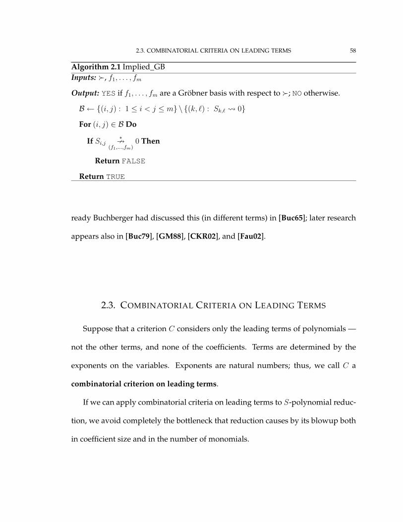
Algorithm 2.1 Implied_GBInputs: �, f1, . . . , fm
Output: YESif f1, . . . , fm are a Gröbner basis with respect to �; NOotherwise.
B ← {(i, j) : 1 ≤ i < j ≤ m} \ {(k, `) : Sk,` 0}
For (i, j) ∈ B Do
If Si,j∗9
(f1,...,fm)0 Then
Return FALSE
Return TRUE
ready Buchberger had discussed this (in different terms) in [Buc65]; later research
appears also in [Buc79], [GM88], [CKR02], and [Fau02].
2.3. COMBINATORIAL CRITERIA ON LEADING TERMS
Suppose that a criterion C considers only the leading terms of polynomials —
not the other terms, and none of the coefficients. Terms are determined by the
exponents on the variables. Exponents are natural numbers; thus, we call C a
combinatorial criterion on leading terms.
If we can apply combinatorial criteria on leading terms to S-polynomial reduc-
tion, we avoid completely the bottleneck that reduction causes by its blowup both
in coefficient size and in the number of monomials.

2.4. THE BUCHBERGER CRITERIA 59
2.4. THE BUCHBERGER CRITERIA
During and after his PhD thesis, Bruno Buchberger presented two combinato-
rial criteria on leading terms.2
BUCHBERGER’S FIRST CRITERION. In his PhD thesis [Buc65] Buchberger had al-
ready discovered the following criterion which allows one to skip some S-poly-
nomial reductions.
THEOREM 2.4. If lt� (fi) and lt� (fj) are relatively prime, then Si,j has a representation
modulo fi, fj .
Before presenting the proof, we encourage the reader to consider again the re-
duction of S1,3 in example 1.32 on page 36. Notice that the leading terms were
relatively prime. Upon careful examination, we see that the reduction took place
with the quotients being the non-leading monomial of f1; we can call such mono-
mials “trailing monomials”. By collecting the quotients into a representation (as in
the proof of lemma 1.28 on page 30), we discern that S1,3 has a form something like
(2.1) S1,3 = R1 · f3 −R3 · f1
2Because our research considers only “combinatorial criteria on the leading terms,” we will refer tothem simply as “combinatorial criteria”.
2.4. THE BUCHBERGER CRITERIA 60
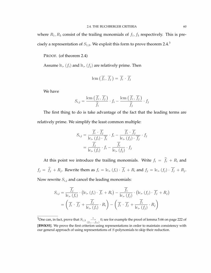
where R1, R3 consist of the trailing monomials of f1, f3 respectively. This is pre-
cisely a representation of S1,3. We exploit this form to prove theorem 2.4.3
PROOF. (of theorem 2.4)
Assume lt� (fi) and lt� (fj) are relatively prime. Then
lcm(fi , fj
)= fi · fj
We have
Si,j =lcm
(fi , fj
)fi
· fi −lcm
(fi , fj
)fj
· fj
The first thing to do is take advantage of the fact that the leading terms are
relatively prime. We simplify the least common multiple:
Si,j =fi · fj
lc� (fi) · fi
· fi −fi · fj
lc� (fj) · fj
· fj
=fj
lc� (fi)· fi −
fi
lc� (fj)· fj
At this point we introduce the trailing monomials. Write fi = fi + Ri and
fj = fj + Rj . Rewrite them as fi = lc� (fi) · fi + Ri and fj = lc� (fj) · fj + Rj .
Now rewrite Si,j and cancel the leading monomials:
Si,j =fj
lc� (fi)·(lc� (fi) · fi + Ri
)− fi
lc� (fj)·(lc� (fj) · fj + Rj
)=
(fi · fj +
fj
lc� (fi)·Ri
)−(
fi · fj +fi
lc� (fj)·Rj
)3One can, in fact, prove that S1,3
∗−→(f1,...,fm)
0; see for example the proof of lemma 5.66 on page 222 of
[BWK93]. We prove the first criterion using representations in order to maintain consistency withour general approach of using representations of S-polynomials to skip their reduction.

2.4. THE BUCHBERGER CRITERIA 61
=fj
lc� (fi)·Ri −
fi
lc� (fj)·Rj
Now we introduce additional polynomials that should help us obtain a repre-
sentation similar in form to (2.1):
Si,j =
(fj
lc� (fi)·Ri −
fi
lc� (fj)·Rj
)+
(Ri ·Rj
lc� (fi) · lc� (fj)− Ri ·Rj
lc� (fi) · lc� (fj)
)Some careful rewriting follows:
Si,j =
(fj
lc� (fi) · lc� (fj)·Ri −
fi
lc� (fi) · lc� (fj)·Rj
)
+
(Ri ·Rj
lc� (fi) · lc� (fj)− Ri ·Rj
lc� (fi) · lc� (fj)
)=
1
lc� (fi) · lc� (fj)·(
fj ·Ri + Ri ·Rj
)− 1
lc� (fi) · lc� (fj)·(
fi ·Rj + Ri ·Rj
)=
(1
lc� (fi) · lc� (fj)·Ri
)· fj −
(1
lc� (fi) · lc� (fj)·Rj
)· fi
We now have
Si,j = hifi + hjfj
where
hi = − 1
lc� (fi) · lc� (fj)·Rj
and
hj =1
lc� (fi) · lc� (fj)·Ri

2.4. THE BUCHBERGER CRITERIA 62
Do hi, hj give a representation of Si,j? They will if
hi · fi ≺ lcm(fi , fj
)and
hj · fj ≺ lcm(fi , fj
)Observe that
hi · fi = Rj · fi
≺ fj · fi
= lcm(fi , fj
)Similarly,
hj · fj ≺ lcm(fi , fj
)Hence hi, hj give a representation of Si,j modulo fi, fj . �
BUCHBERGER’S SECOND CRITERION. In [Buc79], Buchberger presented an addi-
tional criterion; this one allows one to skip an S-polynomial reduction based on
the knowledge that others reduce to zero. Buchberger calls this criterion a “chain
criterion,” and we can see why from the form of (A).
THEOREM 2.5. If lt� (fk) | lcm (lt� (fi) , lt� (fj)), then (A)⇒(B) where
(A) Si,k∗−→
(f1,...,fm)0 and Sk,j
∗−→(f1,...,fm)
0.
(B) Si,j has a representation modulo f1, . . . , fm.
2.4. THE BUCHBERGER CRITERIA 63
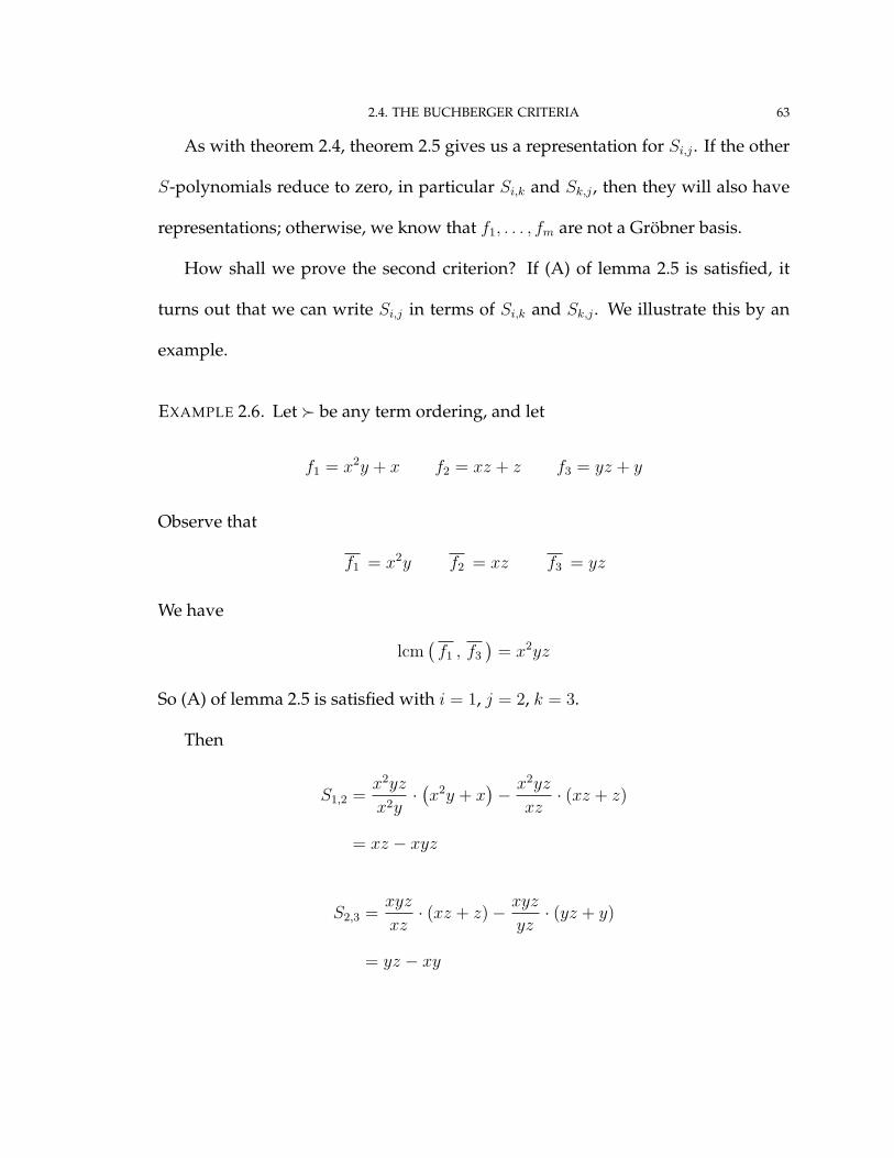
As with theorem 2.4, theorem 2.5 gives us a representation for Si,j . If the other
S-polynomials reduce to zero, in particular Si,k and Sk,j , then they will also have
representations; otherwise, we know that f1, . . . , fm are not a Gröbner basis.
How shall we prove the second criterion? If (A) of lemma 2.5 is satisfied, it
turns out that we can write Si,j in terms of Si,k and Sk,j . We illustrate this by an
example.
EXAMPLE 2.6. Let � be any term ordering, and let
f1 = x2y + x f2 = xz + z f3 = yz + y
Observe that
f1 = x2y f2 = xz f3 = yz
We have
lcm(f1 , f3
)= x2yz
So (A) of lemma 2.5 is satisfied with i = 1, j = 2, k = 3.
Then
S1,2 =x2yz
x2y·(x2y + x
)− x2yz
xz· (xz + z)
= xz − xyz
S2,3 =xyz
xz· (xz + z)− xyz
yz· (yz + y)
= yz − xy

2.4. THE BUCHBERGER CRITERIA 64
S1,3 =x2yz
x2y·(x2y + x
)− x2yz
yz· (yz + y)
= xz − x2y
We claim that we can write S1,3 in terms of S1,2 and S2,3. Notice that S1,2 and
S1,3 have a monomial in common, xz. While S2,3 and S1,3 do not have a monomial
in common, the monomial −xy can “multiply up” to −x2y. Let’s try combining
S1,2 with the appropriate multiple of S2,3:
S1,2 + x · S2,3 = (xz − xyz) + x · (yz − xy)
= xz − x2y
= S1,3
It worked! What we did was apply a monomial multiple to other S-poly-
nomials, and we could rewrite them to obtain the desired S-polynomial. If S1,2
and S1,3 have representations, then we should be able to combine those represen-
tations in the same way to obtain a representation of S1,3.
How do we find these monomials? This is where Buchberger’s second criterion
becomes necessary: the “magic monomials” derive from
lcm(f1 , f3
)lcm
(f1 , f2
) lcm(f1 , f3
)lcm
(f2 , f3
)Since f2 divides the least common multiple of f1 and f3 , the two quotients above
will be terms and not rational expressions. Inspection shows that in the case of

2.4. THE BUCHBERGER CRITERIA 65
this example, the first quotient is 1, and the second is x; these were the “magic
monomials” that gave us the right combination.
We note that f1, f2, f3 are not a Gröbner basis. There is no need to reduce S1,3 to
verify this, since S1,2 does not reduce to zero. �
We apply this insight to prove the theorem.
PROOF. Assume fk | lcm(fi , fj
).
Assume (A):
Si,k∗−→
(f1,...,fm)0 or Sk,j
∗−→(f1,...,fm)
0
Consider
Si,j =lcm
(fi , fj
)fi
· fi −lcm
(fi , fj
)fj
· fj
To obtain the S-polynomials involving fk, we have to introduce fk to the equa-
tion. We use a multiple of fk that may not remain polynomial if Buchberger’s
second criterion is not satisfied:
Si,j =
(lcm
(fi , fj
)fi
· fi −lcm
(fi , fj
)fj
· fj
)
+
(lcm
(fi , fj
)fk
· fk −lcm
(fi , fj
)fk
· fk
)
=
(lcm
(fi , fj
)fi
· fi −lcm
(fi , fj
)fk
· fk
)
+
(lcm
(fi , fj
)fk
· fk −lcm
(fi , fj
)fj
· fj
)

2.4. THE BUCHBERGER CRITERIA 66
At this point we need to massage the equation a little, introducing factors that
will lead us towards writing Si,j in terms of Si,k and Sk,j :
Si,j =lcm
(fi , fk
)lcm
(fi , fk
) ·( lcm(fi , fj
)fi
· fi −lcm
(fi , fj
)fk
· fk
)
+lcm
(fk , fj
)lcm
(fk , fj
) ·( lcm(fi , fj
)fk
· fk −lcm
(fi , fj
)fj
· fj
)
=lcm
(fi , fj
)lcm
(fi , fk
) ·( lcm(fi , fk
)fi
· fi −lcm
(fi , fk
)fk
· fk
)
+lcm
(fi , fj
)lcm
(fk , fj
) ·( lcm(fk , fj
)fk
· fk −lcm
(fk , fj
)fj
· fj
)
=lcm
(fi , fj
)lcm
(fi , fk
) · Si,k +lcm
(fi , fj
)lcm
(fk , fj
) · Sk,j
Recall that Si,k∗−→
(f1,...,fm)0 and Sk,j
∗−→(f1,...,fm)
0. By lemma 1.28, there exist h1 . . . , hm
such that h1, . . . , hm give a representation of Si,k. Also, there exist H1, . . . , Hm such
that H1, . . . , Hm give a representation of Sk,j . Then
Si,j =lcm
(fi , fj
)lcm
(fi , fk
) · Si,k +lcm
(fi , fj
)lcm
(fk , fj
) · Sk,j
=lcm
(fi , fj
)lcm
(fi , fk
) · (h1f1 + · · ·+ hmfm) +lcm
(fi , fj
)lcm
(fk , fj
) · (H1f1 + · · ·+ Hmfm)
Collecting along f1, . . . , fm, we have
Si,j =
(lcm
(fi , fj
)lcm
(fi , fk
) · h1 +lcm
(fi , fj
)lcm
(fk , fj
) ·H1
)· f1
+ · · ·+
(lcm
(fi , fj
)lcm
(fi , fk
) · hm +lcm
(fi , fj
)lcm
(fk , fj
) ·Hm
)· fm

2.4. THE BUCHBERGER CRITERIA 67
For ` = 1, . . . ,m let
H` =lcm
(fi , fj
)lcm
(fi , fk
) · h` +lcm
(fi , fj
)lcm
(fk , fj
) ·H`
Then
Si,j = H1 · f1 + · · ·+Hm · fm
For ` = 1, . . . ,m,H` 6= 0 implies
H` · f` =
(lcm
(fi , fj
)lcm
(fi , fk
) · h` +lcm
(fi , fj
)lcm
(fk , fj
) ·H`
)· f`
= max�
(lcm
(fi , fj
)lcm
(fi , fk
) · h` · f` ,lcm
(fi , fj
)lcm
(fk , fj
) · H` · f`
)
Recall that the hk are a representation for Si,k and the Hk are a representation for
Sk,j . Thus
H` · f` ≺ max
(lcm
(fi , fj
)lcm
(fi , fk
) · lcm ( fi , fk
),
lcm(fi , fj
)lcm
(fk , fj
) · lcm ( fk , fj
))
= lcm(fi , fj
)We see thatH1, . . . ,Hm give a representation of Si,j modulo f1, . . . , fm. �
We should issue a cautionary note. Unlike the footnote to theorem 2.4 on
page 59, Buchberger’s second criterion does not guarantee that Si,j reduces to zero;
it only guarantees that we do not need to check whether it does. It is entirely pos-
sible that Si,j does not reduce to zero! In this case, it is certain that one of Si,k or Sk,j
also does not reduce to zero. Since the computation of Si,k and Sk,j are already
necessary to Buchberger’s algorithm, there is no need to check Si,j .

2.4. THE BUCHBERGER CRITERIA 68
We illustrate this warning with example 2.7.
EXAMPLE 2.7. Let f1 = x2y +x, f2 = xy, and f3 = x3. Let� be any admissible term
ordering. Then
f1 = x2y f2 = xy f3 = x3
Observe that
f2 | lcm(f1 , f3
)So S1,3 0.
However,
S1,3 =lcm (x2y, x3)
x2y·(x2y + x
)− lcm (x2y, x3)
x3· x3
= x ·(x2y + x
)− y · x3
= x2
Clearly S1,3 9(f1,f2,f3)
, so
S1,3∗9
(f1,f2,f3)0
As expected, the chain that f2 should build does not hold at S1,2:
S1,2 =lcm (x2y, xy)
x2y·(x2y + x
)− lcm (x2y, xy)
xy· xy
= 1 ·(x2y + x
)− x · xy
= x

2.4. THE BUCHBERGER CRITERIA 69
and S1,2 9(f1,f2,f3)
, so
S1,2∗9
(f1,f2,f3)0
Since S1,2 does not reduce to zero, it should not surprise us that S1,3 does not reduce
to zero. �
SUMMARY. To summarize, we provide the following definition:
DEFINITION 2.8. Buchberger’s combinatorial criteria are
BC1 (t1, t3) ⇔ gcd (t1, t3) = 1
BC2 (t1, t2, t3) ⇔ t2 | lcm (t1, t3)
We now have the following corollary to theorems 2.4 and 2.5:
COROLLARY 2.9.
BC1 (t1, t3) or BC2 (t1, t2, t3) ⇒ S1,3 0
We conclude this section with an example illustrating the efficacy of Buch-
berger’s criteria.
EXAMPLE 2.10. Let �= lex (x, y, z) and4
f1 = x + y + z
4This system derives from Cyclic-3, a Gröbner basis benchmark related to the roots of the cyclicpolynomial X3 − 1 = 0.
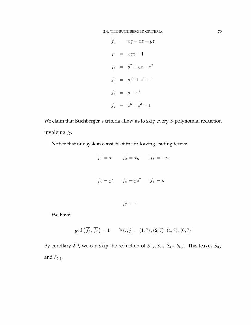
2.4. THE BUCHBERGER CRITERIA 70
f2 = xy + xz + yz
f3 = xyz − 1
f4 = y2 + yz + z2
f5 = yz2 + z3 + 1
f6 = y − z4
f7 = z6 + z3 + 1
We claim that Buchberger’s criteria allow us to skip every S-polynomial reduction
involving f7.
Notice that our system consists of the following leading terms:
f1 = x f2 = xy f3 = xyz
f4 = y2 f5 = yz2 f6 = y
f7 = z6
We have
gcd(fi , fj
)= 1 ∀ (i, j) = (1, 7) , (2, 7) , (4, 7) , (6, 7)
By corollary 2.9, we can skip the reduction of S1,7, S2,7, S4,7, S6,7. This leaves S3,7
and S5,7.
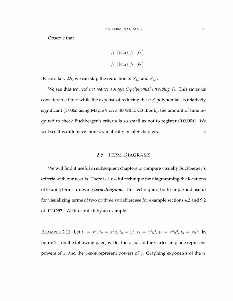
2.5. TERM DIAGRAMS 71
Observe that
f1 | lcm(f3 , f7
)f6 | lcm
(f5 , f7
)By corollary 2.9, we can skip the reduction of S3,7 and S5,7.
We see that we need not reduce a single S-polynomial involving f7. This saves us
considerable time: while the expense of reducing these S-polynomials is relatively
significant (1.080s using Maple 9 on a 400MHz G3 iBook), the amount of time re-
quired to check Buchberger’s criteria is so small as not to register (0.0000s). We
will see this difference more dramatically in later chapters. �
2.5. TERM DIAGRAMS
We will find it useful in subsequent chapters to compare visually Buchberger’s
criteria with our results. There is a useful technique for diagramming the locations
of leading terms: drawing term diagrams. This technique is both simple and useful
for visualizing terms of two or three variables; see for example sections 4.2 and 9.2
of [CLO97]. We illustrate it by an example.
EXAMPLE 2.11. Let t1 = x3, t2 = x2y, t3 = y5, t4 = x4y2, t5 = x2y2, t6 = xy4. In
figure 2.1 on the following page, we let the x-axis of the Cartesian plane represent
powers of x, and the y-axis represent powers of y. Graphing exponents of the tk

2.5. TERM DIAGRAMS 72
4
2
t4
64
t6
1
t10
6
0 3
3
x
2t5
1
y
t3
5
t2
5
Figure 2.1: Term diagram of t1, t2, . . . , t6
as though they were points, we can visualize where the terms appear in relation to
each other.
Obviously, if one term is further to the left of a second, and further below it,
then the first term divides the second. We see that illustrated with t1 and t4: t1
is both further left and below t4. Thus we have a visual clue that t1 | t4. We also
see this illustrated with t2 and t5. However, t6 is not divisible by another of the tk,
which we see in the diagram because it does not lie both further left and below any
of t1, . . . , t5.
Figure 2.2 on the next page illustrates this divisibility more clearly by shading
the northeast quadrant of each term. Any term in a shaded quadrant that lies away
from the southwest corner is divisible by the term that does lie in that southwest
corner. In figure 2.2, both t4 and t5 lie away from the southwest corner of a shaded
quadrant (in fact, t4 lies in a veritable sea of shading). Since the southwest corner
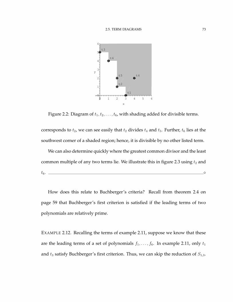
2.5. TERM DIAGRAMS 73
2
yt5
6
t3
3
2
6
5
0
4
5
t6
1
x
10
t2
4
t1
3
t4
Figure 2.2: Diagram of t1, t2, . . . , t6, with shading added for divisible terms.
corresponds to t2, we can see easily that t2 divides t4 and t5. Further, t6 lies at the
southwest corner of a shaded region; hence, it is divisible by no other listed term.
We can also determine quickly where the greatest common divisor and the least
common multiple of any two terms lie. We illustrate this in figure 2.3 using t2 and
t6. �
How does this relate to Buchberger’s criteria? Recall from theorem 2.4 on
page 59 that Buchberger’s first criterion is satisfied if the leading terms of two
polynomials are relatively prime.
EXAMPLE 2.12. Recalling the terms of example 2.11, suppose we know that these
are the leading terms of a set of polynomials f1, . . . , f6. In example 2.11, only t1
and t3 satisfy Buchberger’s first criterion. Thus, we can skip the reduction of S1,3.
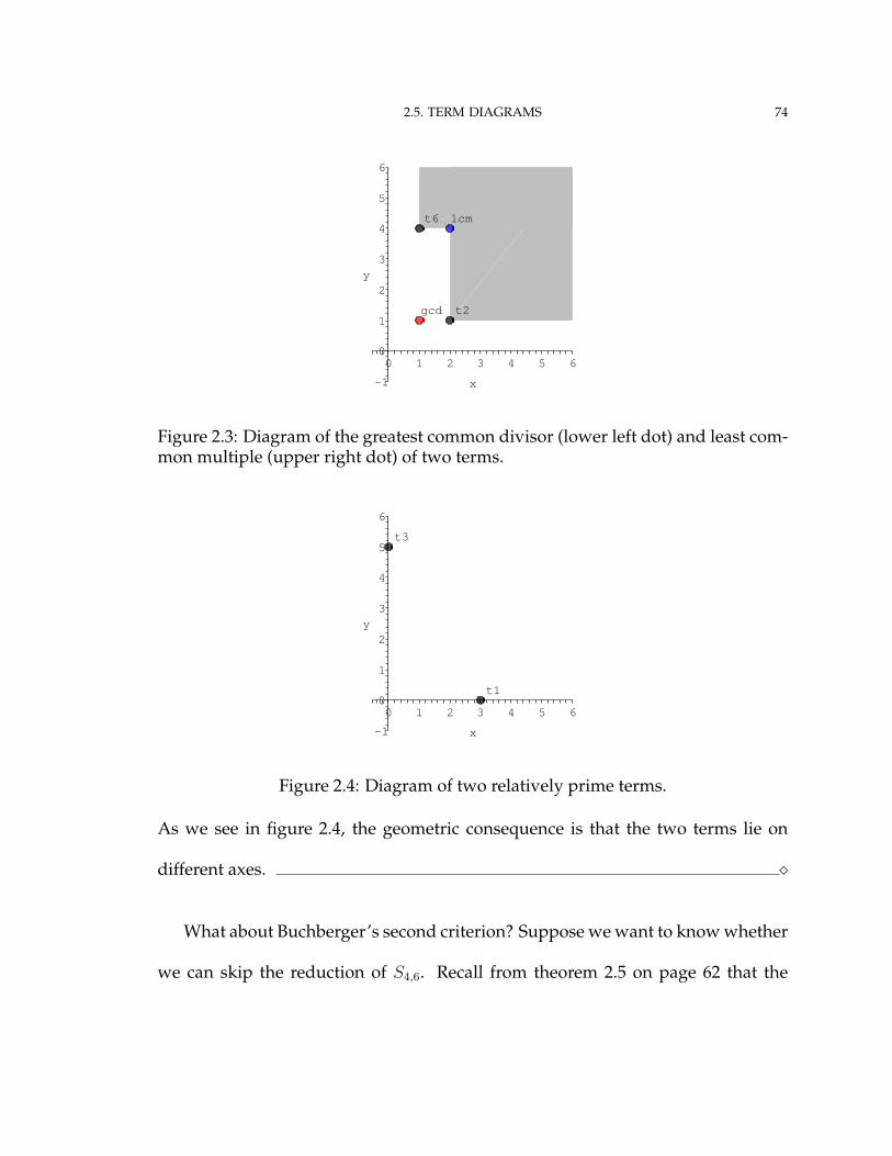
2.5. TERM DIAGRAMS 74
t21
3
60 4
2
5
gcd
4
6
x
5
lcmt6
210
-1
3
y
Figure 2.3: Diagram of the greatest common divisor (lower left dot) and least com-mon multiple (upper right dot) of two terms.
t1
x
05 62 4
y
6
5
4
3
2
1
-1
310
t3
Figure 2.4: Diagram of two relatively prime terms.
As we see in figure 2.4, the geometric consequence is that the two terms lie on
different axes. �
What about Buchberger’s second criterion? Suppose we want to know whether
we can skip the reduction of S4,6. Recall from theorem 2.5 on page 62 that the
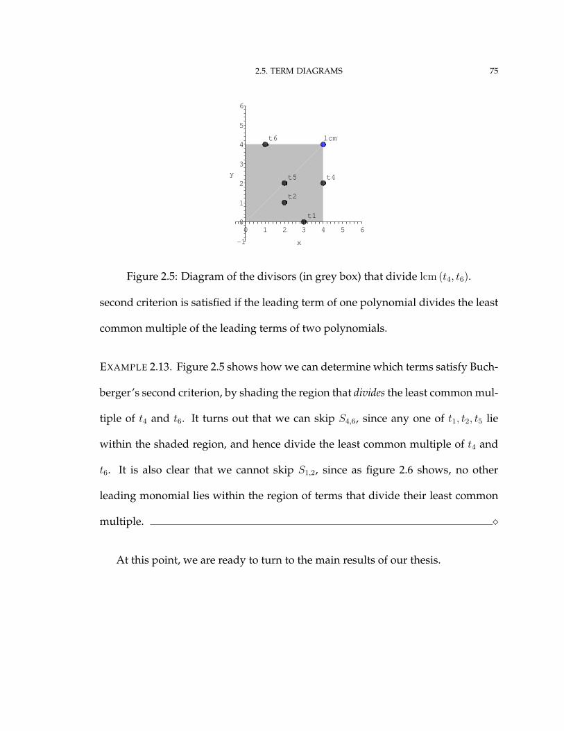
2.5. TERM DIAGRAMS 75
0
4
t1
y t5
x
2
lcm
1 3
5
3
t42
5
t2
6
0
-1
t6
4 6
1
Figure 2.5: Diagram of the divisors (in grey box) that divide lcm (t4, t6).
second criterion is satisfied if the leading term of one polynomial divides the least
common multiple of the leading terms of two polynomials.
EXAMPLE 2.13. Figure 2.5 shows how we can determine which terms satisfy Buch-
berger’s second criterion, by shading the region that divides the least common mul-
tiple of t4 and t6. It turns out that we can skip S4,6, since any one of t1, t2, t5 lie
within the shaded region, and hence divide the least common multiple of t4 and
t6. It is also clear that we cannot skip S1,2, since as figure 2.6 shows, no other
leading monomial lies within the region of terms that divide their least common
multiple. �
At this point, we are ready to turn to the main results of our thesis.

2.5. TERM DIAGRAMS 76
5
t5
20
6
5
y
4
t2
6
t1
2
1
1
x
04
-1
t4
t3
t6
3
3
Figure 2.6: No other monomial lies within the region of divisors of t1 and t2.

Part 2
New combinatorial criteria for skipping
S-polynomial reduction

Chapter 3
Outline of part two
3.1. BUCHBERGER’S CRITERIA REVISITED
Recall Buchberger’s criteria from definition 2.8 on page 69. We observed that
Buchberger’s criteria are both combinatorial and sufficient for skipping S-poly-
nomial reduction.
Two natural questions to ask are,
• How are Buchberger’s criteria sufficient?
• Are Buchberger’s criteria necessary?
Related to the second question is a third,
• If Buchberger’s criteria are not necessary, what are the complete combi-
natorial criteria that allow us to skip S-polynomial reductions?
78

3.1. BUCHBERGER’S CRITERIA REVISITED 79
The answers to these questions are not immediately obvious. As noted in section
2.2, there has been some research related to this question; [GM88] applies Buch-
berger’s criteria in a modified algorithm to compute Gröbner bases, and [CKR02]
shows that Buchberger’s criteria generate minimal bases of syzygy modules, which
have a parallel with representations of S-polynomials.1 Somewhat further afield is
the work of Jean-Charles Faugère [Fau02] who has found non-combinatorial crite-
ria that allow one to skip S-polynomial reduction.
We can add the following questions:
• How often do Buchberger’s criteria allow us to skip S-polynomial reduc-
tion?
• How many Gröbner bases do not satisfy Buchberger’s criteria?
We will not consider these latter questions rigorously, but we do have some in-
teresting experimental results. They suggest that Buchberger’s criteria arise quite
often. This corresponds with example 2.10 on page 69, where Buchberger’s crite-
ria allowed us to skip all six reductions involving an S-polynomial of f7. (They
would have allowed us to skip a great deal more, as well.) We present surveys of
randomly-generated polynomials in sections 4.3.3, 5.3.3, and 6.3.3.
1For example, [CLO97] proves Buchberger’s second criterion (our corollary 2.9 on page 69) usingsyzygies (their proposition 10 on page 106).

3.2. FORMAL STATEMENT OF THE PROBLEM IN PART TWO 80
3.2. FORMAL STATEMENT OF THE PROBLEM CONSIDERED IN PART
TWO
To answer the questions posed in section 3.1, we need to formalize the problem.
The following definition provides the structure that guides the remainder of part
2.
DEFINITION 3.1. We define CC, the “complete combinatorial criterion,” as follows:
Inputs: t1, . . . , tm,�,P ⊂ {(i, j) : 1 ≤ i < j ≤ m}
Output: the boolean value of[∀ (i, j) ∈ P Si,j
∗−→(f1,...,fm)
0
]⇓
GB� (f1, . . . , fm)
∀f1, . . . , fm such that fk = tk
What does this say?
First, CC is a test on leading terms, not on coefficients or on other terms. So one
of its proper inputs is a list of terms t1, . . . , tm, not a list of polynomials f1, . . . , fm.
In consequence, CC provides a guarantee about every set of polynomials f1, . . . , fm
with leading terms t1, . . . , tm.
3.2. FORMAL STATEMENT OF THE PROBLEM IN PART TWO 81
What is this guarantee? Criterion CC guarantees that if the S-polynomials listed
in P reduce to zero, then f1, . . . , fm are a Gröbner basis. In other words, we can skip
the reductions of those S-polynomials not indexed by P .
On the other hand, if CC is false, then we know that there exists some system
f1, . . . , fm with leading terms t1, . . . , tm, but f1, . . . , fm are not a Gröbner basis. In
other words, we would need more information than the leading terms alone to
decide whether polynomials with leading terms t1, . . . .tm are a Gröbner basis.
Notice that, given t1, . . . , tm, we cannot try a brute-force method of testing every
set of polynomials f1, . . . , fm with those leading terms; we cannot even make a list
of all such f1, . . . , fm: there are infinitely many!
How is CC related to the definition of skipping S-polynomial reduction (definition 2.2
on page 55)? It can substitute for C in the definition of skipping S-polynomial re-
duction. Because of this, CC does not guarantee that every S-polynomial reduces
to zero; so, it does not guarantee that f1, . . . , fm are a Gröbner basis; it merely guar-
antees that we need not include Si,j in the set P of S-polynomials whose reduction
we check. Using the notation of algorithm Implied_GB ( 2.1 on page 58), CC
guarantees only that (i, j) 6∈ B.
Of course, we might be able to skip S-polynomial reductions for some sys-
tems f1, . . . , fm where CC is not satisfied. This is because CC is a condition on the
leading terms only: in order to show that CC is not true, it suffices to find poly-
nomials f1, . . . , fm with the specified leading terms, one of whose S-polynomials
3.3. OUTLINE OF THE REMAINDER OF PART TWO 82
does not reduce to zero. However, because S-polynomial reduction depends also
on the trailing monomials, it may well be that we can skip the reduction of Si,j
even though it does not reduce to zero.
3.3. OUTLINE OF THE REMAINDER OF PART TWO
Now that we have defined the problem formally, we proceed in a systematic
manner by increasing the size of P :
• in chapter 4, we set P = ∅, and thus present criteria that decide
whether we can skip all S-polynomial reductions;
• in chapter 5, we set P = {(1, 2)}, and thus present criteria that
decide whether we can skip all but one S-polynomial reductions;
• in chapter 6, we set m = 3 and P = {(1, 2) , (2, 3)}, so that given
f1, f2, f3, we can use the criterion presented in that chapter to de-
cide whether we can skip all but one S-polynomial reductions.
Things become somewhat difficult when we consider skipping all but two S-poly-
nomial reductions. We provide a complete criterion for m = 3, where m is the
number of polynomials, but the more general question for m > 3 remains open.
The problem also remains open for any m when the size of P is larger than two.

3.4. AN INVALUABLE LEMMA 83
3.4. AN INVALUABLE LEMMA
We will find it necessary in chapters 4, 5, and 6 to construct sets of polynomials
f1, . . . , fm that serve as counterexamples in the following way: the leading terms
f1 , . . . , fm do not satisfy CC, and f1, . . . , fm are not a Gröbner basis. How do we
prove that f1, . . . , fm are not a Gröbner basis? By theorem 1.30, we need to find
i 6= j such that Si,j∗9
(f1,...,fm)0.
A great help towards this end would be a clear form for such a counterexample
f1, . . . , fm. Lemma 3.2 provides this form for chapters 4 and 5. In chapter 6 we ap-
ply this lemma for one counterexample (lemma 6.8 on page 131), but require a gen-
eralized form of the lemma for another group of counterexamples (lemma 6.9 on
page 134).
LEMMA 3.2. Let τ be a nonzero monomial, and F = (f1, . . . , fm) a system of polynomials.
Then (A)⇒(B) where
(A) ∃µ with 1 ≤ µ ≤ m such that [ (A1) and (A2) ] where
(A1) f` - τ ∀` = 1, . . . , µ
(A2) ∀` = µ + 1, . . . ,m
f` = t` + u` with t` 6= u`
u` | t`
(B) τ∗9F
0.
Before proving the lemma, we illustrate it with the following example.

3.4. AN INVALUABLE LEMMA 84
EXAMPLE 3.3. Let p1 = xy, f1 = y− 1, f2 = x2. Let� be an arbitrary term ordering.
We have
f1 = y f2 = x2
Clearly p1 9f2
, since degx f2 > degx p1. Observe that
p1 −→f1
x
Write p2 = x. We still have p2 9f2
.
Why? Since the leading monomial of f1 cancels the monomial p1, the remain-
der p2 is determined by the trailing term of f1. Comparing the two terms of the
binomial f1, we see degx y ≥ degx 1. As a consequence, degx p2 ≤ degx p1 < degx f2 .
Hence p2 9f2
; in fact, p2 9(f1,f2)
, and p2 is the only possible reduction of p1 over f1, f2.
Thus p1∗9
(f1,f2)0. �
The application of lemma 3.2 will occur after we construct fi, fj such that Si,j
is a monomial; then we set τ = Si,j . A permutation on the polynomial indices
1, . . . ,m will sometimes be required for a rigorous application of the lemma; we
indicate the necessary permutation in the text.
PROOF. Let τ0, . . . , τs be an arbitrary reduction chain of τ modulo F :
τ = τ0 −→F
τ1 −→F· · · −→
Fτs 9
F
We claim that ∀k = 0, . . . , s, τk is a nonzero monomial and f` - τk ∀` = 1, . . . , µ.
We proceed by induction.

3.4. AN INVALUABLE LEMMA 85
Inductive base: Observe that τ0 = τ , so τ0 is a nonzero monomial, and f` - τ0
∀` = 1, . . . , µ.
Inductive step: Assume that τk is a nonzero monomial, and f` - τk ∀` =
1, . . . , µ. We will show that τk+1 is a nonzero monomial, and f` - τk+1 for all ` =
1, . . . , µ.
We have f` - tk for ` = 1, . . . ,m.
Then τk −→fj
τk+1 implies µ + 1 ≤ j ≤ m.
Let ` ∈ {1, . . . ,m} be arbitrary, but fixed.
Since f` - τk, ∃λ such that degxλf` > degxλ
τk.
Since u` | t`, degxλu` ≤ degxλ
t`.
We have
degxλτk+1 = degxλ
(τk
tj· uj
)≤ degxλ
(τk
tj· tj)
= degxλτk
Hence f` - τk+1.
Since k was arbitrary, τk 6= 0 and f` - τk ∀` = 1, . . . , µ ∀k = 0, . . . , s.
Since the reduction chain was arbitrary, τ∗9F
0. �
Now we can address the first question: when can we skip all S-polynomial
reductions?

Chapter 4
Skipping all S-polynomial reductions
4.1. PROBLEM
It follows from Buchberger’s first criterion that if the leading terms of f1, . . . , fm
are all pairwise relatively prime, then we can skip the reduction of their S-poly-
nomials (see corollary 2.9 on page 69). Two questions arise:
• If the leading terms of two polynomials are not relatively prime,
can we use Buchberger’s second criterion to skip the correspond-
ing S-polynomial, and thus skip all S-polynomials reductions?
• Do there exist other combinatorial criteria that would allow us to
skip all S-polynomial reductions?
Stated formally, we are looking for an algorithm that decides
CC (t1, . . . , tm,�, ∅)
86

4.2. RESULT 87
By definition 3.1 on page 80, this would be equivalent to an algorithm that decides
GB� (f1, . . . , fm) ∀f1, . . . , fm such that f1 = t1, . . . , fm = tm
The answer is given by algorithm 4.1 on page 90, which follows from theorem 4.1.
4.2. RESULT
THEOREM 4.1. (A) is equivalent to (B) where
(A) GB� (f1, . . . , fm) for all f1, . . . , fm such that f1 = t1, . . ., fm = tm
(B) [ (B1) or (B2) ] where
(B1) gcd (ti, tj) = 1 ∀i 6= j
(B2) tk = 1 ∃k
A few observations before we prove theorem 4.1:
That (A)⇐(B) is obvious: clause (B1) is Buchberger’s first criterion, and we
apply corollary 2.9 on page 69; clause (B2) is a “trivial” combinatorial criterion: if
fk = 1, then fk is constant, so every S-polynomial will reduce to zero over fk.
It is not so obvious that (A)⇒(B). To begin with, Buchberger’s second criterion
makes only a trivial contribution to skipping every S-polynomial reduction. Fur-
ther, the theorem asserts that there are no other combinatorial criteria for skipping
every S-polynomial reduction, and this was not exactly clear to start with.
The proof that (A)⇒(B) is also not obvious. Our approach is to show the con-
trapositive: ¬(A)⇐¬(B). This means we have to find a system f1, . . . , fm such that
4.2. RESULT 88
¬GB� (f1, . . . , fm). If we picked a random system f1, . . . , fm, we could reason-
ably expect ¬GB� (f1, . . . , fm). However, this would be hard to prove, since we
would have to trace all possible reductions for a random, unstructured system of
polynomials. What we do, then, is provide a simple, structured counterexample.
Lemma 3.2 on page 83 becomes very useful at this point.
PROOF. (Of theorem 4.1, (A)⇒(B).)
We show the contrapositive: assume ¬(B). Then ¬(B1) and ¬(B2): there exist
i 6= j such that gcd (ti, tj) 6= 1, and ∀k tk 6= 1. We will show ¬(A).
Let
fi = ti
fk = tk + 1 ∀k 6= i
Observe
Si,j =lcm (ti, tj)
ti· ti −
lcm (ti, tj)
tj· (tj + 1)
= lcm (ti, tj)− lcm (ti, tj)−lcm (ti, tj)
tj
= − lcm (ti, tj)
tj
Since
lcm (ti, tj) =titj
gcd (ti, tj)
4.3. APPLICATION OF RESULT 89
we have
Sti,tj = − tigcd (ti, tj)
Since gcd (ti, tj) 6= 1, fi - Si,j .
Applying lemma 3.2, Si,j∗9
(f1,...,fm)0. (The permutation that we need to apply for
the lemma is (1 i) (2 j) – that is, exchange 1 with i and 2 with j, with µ = 1.)
Hence (A)⇒(B). �
4.3. APPLICATION OF RESULT
In this section we illustrate how to apply theorem 4.1 and how not to apply it;
then we consider some experimental results.
4.3.1. AN ALGORITHM FOR THEOREM 4.1. Algorithm 4.1 implements the result.
It checks whether any term is constant, then checks whether every pair of terms is
relatively prime. Since clause (B) considers only the leading terms – not the term
ordering, and not the trailing monomials – we only need to provide these leading
terms as the inputs of algorithm Can_Skip_All_SPolys . In an application, the
user would first calculate the leading terms t1, . . . , tm of f1, . . . , fm with respect to
�; then she would pass these leading terms to the implementation of algorithm
4.1.
4.3.2. EXAMPLES OF THEOREM 4.1.

4.3. APPLICATION OF RESULT 90
Algorithm 4.1 Can_Skip_All_SPolys
Inputs: t1, . . . , tm
Output: YES if we can skip all S-polynomial reductions for all polynomials withleading terms t1, . . . , tm; NOotherwise
For i = 1, . . . ,m
If ti = 1 Then
Return YES
B ← {(i, j) : 1 ≤ i < j ≤ m}
For (i, j) ∈ B
If gcd (ti, tj) 6= 1 Then
Return NO
Return YES
EXAMPLE 4.2. Let f1 = x + 2y + 3z − 1, f2 = y − z + 3, f3 = z + 4. The reader may
notice that f1, f2, f3 are linear, and in triangular form.
We consider two different term orderings. If �= lex (x, y, z), then
f1 = x f2 = y f3 = z
We see that all the leading terms are relatively prime; by theorem 4.1, we can con-
clude that f1, f2, f3 are a Gröbner basis with respect to �without checking a single
S-polynomial. This agrees with the triangular form of the linear system.
In the second case, let �= lex (x, z, y). At this point, the leading term of f2
changes to z, so that the leading terms of f2 and f3 are no longer relatively prime.

4.3. APPLICATION OF RESULT 91
None of the leading terms is 1. Applying theorem 4.1, we see that we cannot con-
clude that f1, f2, f3 are a Gröbner basis with respect to �. In fact,
S2,3 =lcm (z, z)
−z· (y − z + 3)− lcm (z, z)
z· (z + 4)
= −1 · (y − z + 3)− (z + 4)
= −y − 7
None of the monomials of S2,3 is divisible by the leading term of any of f1, f2, f3, so
that f1, f2, f3 are not a Gröbner basis with respect to �. In this case, the triangular
form of the linear system does not guarantee a Gröbner basis, because the second
term ordering prioritizes the pivots differently. The corresponding coefficient ma-
trix is clearly not upper triangular:1 3 2
0 −1 1
0 1 0
�
Since theorem 4.1 considers only the leading terms, we expect to find polyno-
mial systems whose leading terms do not satisfy its hypotheses even though the
polynomials are themselves a Gröbner basis. Our second example illustrates this.
EXAMPLE 4.3. Let f1 = xy + bx, f2 = x2 − bx. Let � be any term ordering on terms
in x and y. Notice that b is constant in this term ordering. The leading terms of the
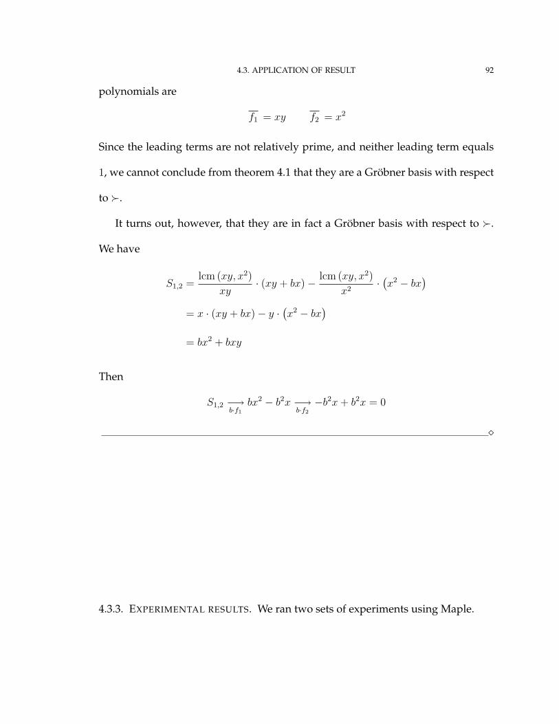
4.3. APPLICATION OF RESULT 92
polynomials are
f1 = xy f2 = x2
Since the leading terms are not relatively prime, and neither leading term equals
1, we cannot conclude from theorem 4.1 that they are a Gröbner basis with respect
to �.
It turns out, however, that they are in fact a Gröbner basis with respect to �.
We have
S1,2 =lcm (xy, x2)
xy· (xy + bx)− lcm (xy, x2)
x2·(x2 − bx
)= x · (xy + bx)− y ·
(x2 − bx
)= bx2 + bxy
Then
S1,2 −→b·f1
bx2 − b2x −→b·f2
−b2x + b2x = 0
�
4.3.3. EXPERIMENTAL RESULTS. We ran two sets of experiments using Maple.
4.3. APPLICATION OF RESULT 93
HOW DOES THEOREM 4.1 APPLY UNDER DIFFERENT CONDITIONS? In the first ex-
periment, we tested how often theorem 4.1 would allow us to skip every S-poly-
nomial reduction. Given a random set of polynomials, we expect that all the lead-
ing terms will be relatively prime only rarely, and the data did not provide any sur-
prises here! On the other hand, changing certain parameters (the term ordering,
the total degree, and the number of variables) provided some interesting insight.
The program we wrote chose polynomials using Maple’s randpoly() with
the following parameters:
we looped from n = 2 to n = 6 variables
for each n, we looped from d = 10 to d = 10n,
where d was the maximum degree of a term,
incrementing d by n with each iteration
for each value of d, we generated 100,000 sets of polynomials
each set consisted of at least 2, at most n sparse polynomials
number of terms per polynomial: rand(2..20)
coefficients: rand(-99..99)
exponents: rand(0..5)
For each set of at most n polynomials, we computed the leading terms with
respect to a fixed term ordering, either total-degree or lexicographic. If every pair
of leading terms was relatively prime, we knew from theorem 4.1 that the set was
a Gröbner basis.

4.3. APPLICATION OF RESULT 94
Why did we restrict each set of polynomials to at most n (the number of vari-
ables)? If there are n variables, then n + 1 polynomials cannot all be relatively
prime, so there is no point in testing the theorem there: for all systems with n + 1
or more polynomials, we will have to check at least one S-polynomial reduction.
We used Maple’s time() command to keep track of how much time we spent
evaluating whether the leading terms were relatively prime. In nearly all cases,
the sum of these times over all 100,000 sets of polynomials for each n and d was
reported as 0 seconds. The only exception was when n = 6 and d = 58; in this very
last case, the software spent 0.009 seconds in evaluation.1
It should come as no surprise that the leading terms of every pair of polynomials
are almost never relatively prime. We see this illustrated in tables 4.1 (when the
term ordering is total-degree) and 4.2 (when the term ordering is lexicographic).
For a total-degree term ordering and only two variables, we get a relatively
high frequency of success when the total degree is low: about 1.5% of the sets of
polynomials for total degree d = 10. Naturally, the frequency of success decreases
as we increase the total degree, since a higher total degree means that the terms
can contain more variables. We have less than 0.5% success when the total degree
is 20.
1Maple’s time() command only keeps track of the amount of time spent in evaluation, and not insimplification. It certainly took much more than zero seconds to run the program; in fact, it tookabout a day. However, whatever time that simplification would add is dwarfed by the amount ofsimplification in polynomial reduction: see for example table 4.4.

4.3. APPLICATION OF RESULT 95
Table 4.1: Number of sets of polynomials where every pair of leading terms isrelatively prime, out of 100,000 sets.
d = 10 d = 10 + n d = 10 + 2n d = 10 + 3n d = 10 + 4nn = 2 1507 1174 882 683 577n = 3 910 470 264 178 103n = 4 569 190 97 44 31n = 5 407 92 33 15 5n = 6 338 44 14 6 1
d = 10 + 5n d = 10 + 6n d = 10 + 7n d = 10 + 8nn = 2 486n = 3 67 49n = 4 13 8 12n = 5 0 3 3 2n = 6 0 0 0 0
(n variables; 2 . . . n polynomials per set; d the maximum degree of a term; expo-nents range from 0 to 5; total-degree term ordering with x1 � · · · � xn)
Table 4.2: Number of sets where every pair of leading terms is relatively prime,out of 100,000 sets.
d = 10 d = 10 + n d = 10 + 2n d = 10 + 3n d = 10 + 4nn = 2 145 86 54 42 30n = 3 67 31 18 8 2n = 4 65 14 9 3 1n = 5 30 5 1 1 1n = 6 29 8 1 0 0
d = 10 + 5n d = 10 + 6n d = 10 + 7n d = 10 + 8nn = 2 24n = 3 3 0n = 4 0 2 0n = 5 0 0 0 0n = 6 0 0 0 0
(n variables; 2 . . . n polynomials per set; d the maximum degree of a term; expo-nents range from 0 to 5; lexicographic term ordering with x1 � · · · � xn)
4.3. APPLICATION OF RESULT 96
The success rate also drops when we increase the pool of variables. Already
with three variables, the number of times we could skip every S-polynomial re-
duction has dipped below 0.9%, even when d = 10. This came as something of a
surprise to me; I expected that with more variables available per term and a fixed
total degree, the probability of single-variable terms would increase. Apparently
the addition of these single-variable terms is counterbalanced by the large number
of terms that are not single-variable, but have the same total degree. However, this
does not explain everything, as we will see in the following paragraph.
The general pattern of table 4.1 is repeated in table 4.2 where the term ordering
is lexicographic. However, the totals for each case are drastically smaller than
they were in table 4.1. This would seem to be because single-variable terms occur
with high degree. Consider x1x2 + x32: a total-degree term ordering would return
x32 as the leading term, while a lexicographic term ordering would return x1x2 as
the leading term. This latter term, which has more variables, is less likely to be
relatively prime with the leading terms of other polynomials.
My explanations for the observed phenomena may appear inconsistent. In the
first, I argued that although we should have a higher probability of single-variable
terms as we increase n, these do not increase the overall success rate because they
are outweighed by other terms in a total-degree term ordering. In the second,
I argued that, single-variable terms are more likely to be the leading terms of a
polynomial in a total-degree term ordering than in a lexicographic term ordering.

4.3. APPLICATION OF RESULT 97
These two arguments are not, however, inconsistent, because I’m arguing in
two different contexts. For a fixed number of variables n, single-variable terms
of high degree will be favored by the total-degree term ordering, while the given
lexicographic term ordering will favor any term with x1 regardless of the total
degree.
For increasing n, however, the number single-variable terms may increase, but
the test program ordered the indeterminates as
x1 � x2 � · · · � xn
The additional single-variable terms are powers of “less privileged” indetermi-
nates, so that x1x2 � x22 for both term orderings.
WHAT IS THE PROBABILITY OF ENCOUNTERING A GRÖBNER BASIS THAT IS NOT
SKIPPED? The second experiment was designed to get an idea of the probability
that a random set of at most n polynomials will be a Gröbner basis. We also used
the opportunity to compare the timings for checking theorem 4.1 and for reducing
all S-polynomials. The results are given in tables 4.3 and 4.4.
In table 4.3, we computed 1,000 systems of random polynomials with at least
two, at most n polynomials per system, where n is the number of variables. Using
a total-degree term order, we checked combinatorially whether we could skip all
S-polynomial reductions; then we checked by S-polynomial reduction whether
the system was a Gröbner basis. We timed each of these computations.

4.3. APPLICATION OF RESULT 98
Table 4.3: Comparison of the number of Gröbner bases found by S-polynomialreduction, to the number found by applying theorem 4.1.
# vars Skips other GBs time to check skip time to check reduction2 5 3 .70s 165s3 0 0 145.91s* 12015s4 0 0 1.01s 4092s5 0 0 .67s 115s6 0 0 .63s 103s
(1000 total polynomials; n the number of variables; 2 . . . n polynomials per set,where n =#vars; 10×n the maximum degree of a term; exponents range from 0 to5; total-degree term ordering with x1 � · · · � xn)*This number must be a fluke; see the discussion in the text.
Again, almost none of the random polynomials that we generated were Gröb-
ner bases. In fact, the only time we found any Gröbner bases at all was for n = 2
variables. Out of a total of 1,000 polynomials for each value of n, this is not sur-
prising. Why did we keep the total so small? Reduction takes too much time.
Interestingly, theorem 4.1 detected most of the Gröbner bases that we did find
(5 out of 8). Keep in mind that these are unstructured polynomials, so we naturally
do not expect to find many Gröbner bases. In a structured set of polynomials, we
would expect more Gröbner bases to be detected by S-polynomial reduction, and
very few of them to be detected by theorem 4.1.
As expected, the total time to check the conditions of theorem 4.1 was very
small, whereas the time to reduce all S-polynomials to zero was larger by several
orders of magnitude. There was one strange result: for n = 3 variables, we had the
strange result that it took nearly 146 seconds to check the leading terms. I am not

4.3. APPLICATION OF RESULT 99
Table 4.4: Comparison of the number of Gröbner bases found by S-polynomialreduction, to the number found by applying theorem 4.1.
# vars Skips total GBs time to check skip time to check reduction2 17453 25502 .02s 19885.71s3 5952 11005 .03s 37295.14s4 1726 3878 .03s 92538.03s5 416 1237 .03s 252596.89s
(1,000,000 total systems of two polynomials; n the number of variables; 10×#varsthe maximum degree of a term; exponents range from 0 to 5; total-degree termordering with x1 � · · · � xn)
sure why this happened. We ran the tests in sets of 100, and one of the sets took
144.58 seconds. Take that one away, and we have a far more reasonable result:
1.33 seconds. By contrast, the corresponding set of S-polynomial reductions was
not abnormally higher than normal; there were other reductions that were much
higher. We are not sure what caused this; later tests did not show a recurrence.
We do notice that the total time increases from n = 2 through n = 3, then
declines, both for checking theorem 4.1 and for checking the S-polynomial reduc-
tions. This could be due to a larger number of occasions for n = 3 where the
first pair of the leading terms are relatively prime, or where the first computed S-
polynomial reduces to zero; with a higher number of variables, that could be less
likely.
In the second experiment, we held the number of polynomials fixed at m = 2.
This gave us some confidence that the computed Gröbner bases would not take

4.3. APPLICATION OF RESULT 100
too long to compute, so we could use a larger sample size of polynomials.2 The
results are given in table 4.4; clearly, the fixed number of polynomials helped keep
the time to check the combinatorial criteria nearly constant. Again, almost none
of the random polynomial systems were Gröbner bases: at most 2.5% for n = 2.
Again, theorem 4.1 detected most of the Gröbner bases that we found: starting
above 66%, and decreasing to around 33%.
As expected, the total time to check the conditions of theorem 4.1 remains very
small, whereas the time to reduce all S-polynomials to zero grew by several orders
of magnitude.
2As the reader sees from table 4.4, however, we gave up after n = 5.
Chapter 5
Skipping all but one S-polynomial
reductions
5.1. PROBLEM
In chapter 4 we characterized completely the combinatorial criteria that allow
us to skip every S-polynomial reduction. In this chapter, we turn our attention to
the question of skipping all but one S-polynomial reduction: given polynomials
f1, . . . , fm, we want to know if they are a Gröbner basis, but we will only check
one S-polynomial reduction. Without loss of generality, we can assume that the
S-polynomial we do reduce is S1,2. We are looking for an algorithm that decides
CC (t1, . . . , tm,�, {(1, 2)})
101
5.2. RESULT 102
By definition 3.1 on page 80, this is equivalent to[S1,2
∗−→(f1,...,fm)
0 ⇒ GB� (f1, . . . , fm)
]∀f1, . . . , fm such that fk = tk
As in chapter 4, it is fairly clear that satisfying some formulation of Buch-
berger’s first criterion would allow us to skip all but one S-polynomial reduction.
We would also like to know whether Buchberger’s second criterion will help us
to skip all but one S-polynomial reduction, or whether additional criteria on the
leading terms will prove useful.
The answer is given by algorithm 5.1 on page 110, which follows from theorem
5.1.
5.2. RESULT
THEOREM 5.1. (A) is equivalent to (B) where:
(A) S1,2∗−→
(f1,...,fm)0 ⇒ GB� (f1, . . . , fm)
∀f1, . . . fm such that f1 = t1, . . ., fm = tm
(B) (B1) ∨ (B2) ∨ (B3) ∨ (B4) where
(B1) gcd (ti, tj) = 1 ∀ (i, j) 6= (1, 2)
(B2) t1 | t2 and gcd (ti, tj) = 1 ∀i 6= j, i 6= 2, j 6= 2
(B3) t2 | t1 and gcd (ti, tj) = 1 ∀i 6= j, i 6= 1, j 6= 1
(B4) tk = 1 ∃k
A few comments before the proof.

5.2. RESULT 103
As with theorem 4.1 on page 87, we see that no additional combinatorial criteria
figure into theorem 5.1: (B) is a formulation of Buchberger’s two criteria, and the
trivial criterion that some polynomial be constant. Note in particular that clauses
(B2) and (B3) are applications of the first and the second criteria: if t1 | t2, then
certainly t1 | lcm (t2, tk) for all k > 2. As a result, it is fairly obvious that (A)⇐(B).
However, proving (A)⇒(B) is more difficult than it was for theorem 4.1. Again,
we approach via the contrapositive and employ lemma 3.2 on page 83; this time,
however, we need more than one counterexample, because the negation of (B) ex-
pands to several cases. It may be possible to resolve all these cases using only one
counterexample, but if so, we have not found it.
PROOF. (Of theorem 5.1, (A)⇒(B).)
We show the contrapositive: namely, ¬(A)⇐¬(B). So assume ¬(B). Then ¬(B1)
and ¬(B2) and ¬(B3) and ¬(B4).
We will show ¬(A).
From ¬(B1), we know that ∃ (i, j) 6= (1, 2) such that gcd (ti, tj) 6= 1.
From ¬(B4), we know that ∀k tk 6= 1.
By distribution and De Morgan, we know that ¬(B2) ∧ ¬(B3) is logically equiv-
alent to (D1) ∨ (D2) ∨ (D3) ∨ (D4) where
(D1) t1 - t2 and t2 - t1
(D2) t1 - t2 and gcd (ti, tj) 6= 1 ∃i 6= j, i 6= 1, j 6= 1
(D3) t2 - t1 and gcd (ti, tj) 6= 1 ∃i 6= j, i 6= 2, j 6= 2
5.2. RESULT 104
(D4) gcd (ti, tj) 6= 1 ∃i 6= j, i 6= 1, j 6= 1
and gcd (ti, tj) 6= 1 ∃i 6= j, i 6= 2, j 6= 2
We consider each case in turn.
Case 1: (D1) t1 - t2 and t2 - t1
Recall ∃ (i, j) 6= (1, 2) such that gcd (ti, tj) 6= 1. Without loss of generality, j > 2.
We have two subcases.
Case 1a: t1 - tj and t2 - tj .
Let F = (f1, . . . , fm) where
f1 = t1
f2 = t2
fj = tj
fk = tk + 1 for k 6= 1, 2, j
Observe that S1,2∗−→F
0 trivially.
Then
Si,j =lcm (ti, tj)
ti· (ti + 1)− lcm (ti, tj)
tj· tj
= lcm (ti, tj) +lcm (ti, tj)
ti− lcm (ti, tj)
=lcm (ti, tj)
ti
5.2. RESULT 105
Since
lcm (ti, tj) =titj
gcd (ti, tj)
we have
Si,j =tj
gcd (ti, fj)
Obviously Si,j | tj .
Since t1 - tj and Si,j | tj , f1 - Si,j .
Since t2 - tj and Si,j | tj , f2 - Si,j .
Since gcd (ti, tj) 6= 1, fj - Si,j .
By lemma 3.2, Si,j∗9F
0. (Use the permutation (3 j) with µ = 3.)
Case 1b: t1 | tj or t2 | tj
Let F = (f1, . . . , fm) where
f1 = t1
f2 = t2
fk = tk + 1 for k 6= 1, 2
Observe that S1,2∗−→F
0 trivially.
If t1 | tj , then S1,j = −1. Recall tk 6= 1 for k = 1, . . . ,m. So S1,j∗9F
0.
Otherwise, t2 | tj , whence S2,j = −1∗9F
0.
Case 2: (D2) t1 - t2andgcd (ti, tj) 6= 1 ∃i 6= j, i 6= 1, j 6= 1
Without loss of generality, j 6= 2.

5.2. RESULT 106
We have three subcases.
Case 2a: t1 - ti and t2 - ti
This case is proved using a proof similar to that of case 1a, exchanging i and j.
Case 2b: t1 | ti
We note that since t1 - t2 for case 2, i 6= 2.
Let F = (f1, . . . , fm) where
f1 = t1
f2 = t2
fk = tk + 1 for k 6= 1, 2
Observe that S1,2∗−→F
0 trivially.
We have S1,i = −1∗9F
0.
Case 2c: t2 | ti
Let F = (f1, . . . , fm) where
f1 = t1
f2 = t2
fk = tk + 1 for k 6= 1, 2
Observe that S1,2∗−→F
0 trivially.
If i 6= 2, then S2,i = −1. Recall tk 6= 1 for k = 1, . . . ,m; thus S2,i∗9F
0.
5.2. RESULT 107
Otherwise i = 2; consider
S2,j =lcm (t2, tj)
t2· t2 −
lcm (t2, tj)
tj· (tj + 1)
= lcm (t2, tj)− lcm (t2, tj)−lcm (t2, tj)
tj
= − lcm (t2, tj)
tj
Since
lcm (t2, tj) =t2tj
gcd (t2, tj)
we have
S2,j = − t2gcd (t2, tj)
Obviously S2j | t2.
Recall t1 - t2; hence f1 - S2j .
Recall gcd (t2, tj) = gcd (ti, tj) 6= 1; then f2 - S2j .
By lemma 3.2, S2j∗9F
0. (Use µ = 2; no permutation is necessary.)
Case 3: (D3) t2 - t1and gcd (ti, tj) 6= 1 ∃i 6= j, i 6= 2, j 6= 2
This case is symmetric to case 2, so we can prove it symmetrically.
Case 4: (D4) gcd (ti, tj) 6= 1 ∃i 6= j, i 6= 1, j 6= 1
and gcd (ti, tj) 6= 1 ∃i 6= j, i 6= 2, j 6= 2
For the sake of clarity, we rewrite this case as
gcd (ti, tj) 6= 1 ∃i 6= j, i 6= 1, j 6= 1 and gcd (tk, t`) 6= 1 ∃k 6= `, k 6= 2, ` 6= 2

5.3. APPLICATION OF RESULT 108
We have already considered the subcase t1 - t2 in case 2, and the subcase t2 - t1
in case 3. We may assume therefore that t1 | t2 and t2 | t1, or t1 = t2.
We have two subcases.
Case 4a: t1 - ti
This case is proved using a proof similar to that of case 1a, exchanging i and j.
Case 4b: t1 | ti
This case is proved using a proof similar to that of case 1b, exchanging i and j.
For all four cases:
In each case, ∃F such that S12∗−→F
0 but ∃k, ` such that Sk`∗9F
0.
Hence ¬(A). �
5.3. APPLICATION OF RESULT
We present examples of theorem 5.1, then consider some experimental results.
5.3.1. AN ALGORITHM FOR THEOREM 5.1. Implementing an algorithm that de-
cides clause (B) of theorem 5.1 is still rather straightforward, although not so much
as for theorem 4.1; see algorithm 5.1. The extra complication comes from clauses
(B2) and (B3): on the first occasion that we encounter terms t1 and t2 that are not
relatively prime, we need to search for a third term term t3 that divides either t1
or t2. If we cannot find such a term, then (presuming we’ve checked for a constant
polynomial) we can skip all but one S-polynomial reductions only if no other pair

5.3. APPLICATION OF RESULT 109
of terms is relatively prime. The one S-polynomial reduction that we have to check
is S1,2.
If we do find a third term t3 that divides t1 (say), then two things follow imme-
diately: (a) S1,3 is the only S-polynomial that we can skip (since t1 and t3 are clearly
not relatively prime) and (b) we no longer worry whether t1 is relatively prime to
the remaining terms. We do have to worry whether t2 and t3 are relatively prime to
all other terms: if not, then we cannot skip the remaining S-polynomial reductions,
since clause (B) of theorem 5.1 is not satisfied.
As with algorithm 4.1, we only need to pass the leading terms as inputs to our
implementation of theorem 5.1, since clause (B) does not use the term ordering or
any other part of the polynomials.
5.3.2. EXAMPLES OF THEOREM 5.1. We begin with a straightforward example of
when the theorem allows us to skip all but one S-polynomial reductions.
EXAMPLE 5.2. Let
f1 = y2 + 1 f2 = xy3 + 1 f3 = x4 − x2 + 1
Let � be any admissible term ordering. Observe that
f1 = y2 f2 = xy3 f3 = x4
The theorem allows us to skip every S-polynomial reduction except S1,2. Why? We
have

5.3. APPLICATION OF RESULT 110
Algorithm 5.1 Can_Skip_All_But_One_SPolys
Inputs: t1, . . . , tm
Output: YESif we can skip all but one S-polynomial reductions for all polynomialswith leading terms t1, . . . , tm; NOotherwise
Local
number_spolys_cannot_skip← 0
skipped_term← 0
For i = 1, . . . ,m
If ti = 1 Then
Return YES
B ← {(i, j) : 1 ≤ i < j ≤ m}
For (i, j) ∈ B
If gcd (ti, tj) 6= 1 Then
Increment number_spolys_cannot_skip
If number_spolys_cannot_skip > 1 and skipped_term 6= i, j Then
Return NO
Elseif number_spolys_cannot_skip = 1 Then
If Exists k: tk | ti Then
skipped_term← i
B ← B\{(i, `) : ` = 1, . . . ,m}
Elseif Exists k: tk | tj Then
skipped_term← j
B ← B\{(j, `) : ` = 1, . . . ,m}
Return YES

5.3. APPLICATION OF RESULT 111
• f1 | f2
• gcd(f1 , f3
)= 1
This satisfies (B2) of theorem 5.1. Hence, if S1,2∗−→
(f1,f2,f3)0, we have GB� (f1, f2, f3).
As it turns out, S1,2∗9
(f1,f2,f3)0, so f1, f2, f3 are not a Gröbner basis. �
Now we consider two more examples, both featuring the same set of polyno-
mials. We will see how the choice of term ordering, as well as the ordering of the
polynomials, helps determine whether the theorem applies.
EXAMPLE 5.3. Let
f1 = x3y3 + 1 f2 = x5y3z2 − z6 − 1 f3 = z7 + w8 + 1 f4 = z6 + x2z2 + 1
In this example, let �= tdeg (x, y, z, w). We have
f1 = x3y3 f2 = x5y3z2 f3 = w8 f4 = z6
Can we skip every S-polynomial except S1,2?
Under the given term ordering, the leading terms satisfy (B2) of theorem 5.1:
we have
• f1 | f2
• gcd(f1 , f3
)= gcd
(f1 , f4
)= gcd
(f3 , f4
)= 1

5.3. APPLICATION OF RESULT 112
Hence, if S1,2∗−→
(f1,...,f4)0, we know that GB� (f1, . . . , fm). It turns out that we do in
fact have a Gröbner basis here:
S1,2 =lcm (x3y3, x5y3z2)
x3y3·(x3y3 + 1
)− lcm (x3y3, x5y3z2)
x5y3z2·(x5y3z2 − z6 − 1
)= x2z2 ·
(x3y3 + 1
)−(x5y3z2 − z6 − 1
)= z6 + x2z2 + 1
Then
S1,2 −→1·f4
0
�
As noted above, the same polynomials give a different result if we change the
term ordering:
EXAMPLE 5.4. Recall the polynomials of the previous example:
f1 = x3y3 + 1 f2 = x5y3z2 − z6 − 1 f3 = z7 + w8 + 1 f4 = z6 + x2z2 + 1
This time, use �= lex (x, y, z, w). We have
f1 = x3y3 f2 = x5y3z2 f3 = z7 f4 = x2z2
The leading terms of f3 and f4 have changed from the previous example.
To approach this example systematically, let’s trace through algorithm 5.1:
number_spolys_cannot_skip← 0
skipped_term← 0

5.3. APPLICATION OF RESULT 113
B ← {(1, 2) , (1, 3) , (1, 4) , (2, 3) , (2, 4) , (3, 4)}
(i, j) = (1, 2):
Since ti, tj are not relatively prime,
number_spolys_cannot_skip← 1
Since t4 | t1,
skipped_term← 1
B ← {(2, 3) , (2, 4) , (3, 4)}
(i, j) = (2, 3)
Since t2, t3 are not relatively prime,
number_spolys_cannot_skip← 2
Since number_spolys_cannot_skip > 1 and skipped_term 6= 2, 3
Return NO
Under this term ordering, the algorithm finds that we cannot skip all S-poly-
nomials reductions but one.
It remains the case that S1,2 reduces to zero despite the new term ordering.
However, S2,3 does not:
S2,3 =lcm (x5y3z2, z7)
x5y3z2·(x5y3z2 − z6 − 1
)− lcm (x5y3z2, z7)
z7·(z7 + w8 + 1
)= z5 ·
(x5y3z2 − z6 − 1
)− x5y3 ·
(z7 + w8 + 1
)= −z11 − z5 − x5y3w8 − x5y3

5.3. APPLICATION OF RESULT 114
Before showing a reduction path of S2,3, we remind the reader of the leading terms:
f1 = x3y3 f2 = x5y3z2 f3 = z7 f4 = x2z2
Thus
S2,3 −→−x2w8·f1
−z11 − z5 − x5y3 + x2w8
−→−x2·f1
−z11 − z5 + x2w8 + x2
−→−z4·f3
x2w8 + x2 − z5 + z4w8 + z4
9(f1,...,f4)
The remaining reduction paths are nearly identical, although too numerous to list
here. Hence S2,3 9(f1,...,f4)
0. �
5.3.3. EXPERIMENTAL RESULTS. Again, we ran two kinds of experiments: one to
see how often the criteria applied, and one to compare the number of skipped
systems to the number of Gröbner bases.
HOW OFTEN DOES THEOREM 5.1 APPLY? The first thing I noticed when running
experimental results is that the minimum number of polynomials we test should
be three. In my first, naïve attempt to repeat the experiments of section 4.3.3, I ran
a slight modification of the first experiment for theorem 4.1 (see page 93). I did
not change the number of polynomials generated for each turn. Examining the

5.3. APPLICATION OF RESULT 115
Table 5.1: Number of sets where we can skip all but one S-polynomial reduction,out of out of 100,000 sets.
d = 10 d = 10 + n d = 10 + 2n d = 10 + 3n d = 10 + 4nn = 3 314 138 67 44 24n = 4 220 41 15 2 1n = 5 130 24 4 1 1n = 6 86 10 0 0 0
d = 10 + 5n d = 10 + 6n d = 10 + 7n d = 10 + 8nn = 3 16 9n = 4 1 1 0n = 5 0 0 0 0n = 6 0 0 1 0
(n variables; 3 . . . n + 1 polynomials per set; d the maximum degree of a term;exponents range from 0 to 5; total-degree term ordering with x1 � · · · � xn)
preliminary results, I noticed with creeping horror that, for two variables, I was
obtaining “a 100% success rate”, and I began to panic!
I spent a few minutes in frantic debugging before realizing how foolish I had
been: for n = 2 variables, the first program would only test two polynomials. With
a set of two polynomials, there is only one S-polynomial to reduce: S1,2. It comes
as no surprise, then, that for the set f1, f2, we can always skip “every S-polynomial
reduction but one”: S1,2.
A revised program produced more reasonable results; see table 5.1. We gener-
ated the data in the following manner:
we looped from n = 2 to n = 6 variables
for each n, we looped from d = 10 to d = 10n stepping by n
for each value of d, we generated 100,000 sets of polynomials
5.3. APPLICATION OF RESULT 116
each set consisted of at least 3, at most n + 1 sparse polynomials
number of terms per polynomial: rand(2..20)
each term had maximum degree d
coefficients: rand(-99..99)
exponents: rand(0..5)
At this point, I made another mistake: I began comparing the data in table
5.1 with that of table 4.1. Again, I began to panic: one would expect that there
would be more sets of polynomials where we can skip all but one S-polynomial
reduction, than when we can skip all reductions, since fewer leading terms have
to be relatively prime. A naïve comparison of table 5.1 with table 4.1 suggests that
there are fewer sets where we skip all but one S-polynomial reduction.
The reality is that the tables are incomparable due to the number of polyno-
mials in each set. Table 5.1 allows 3 . . . n + 1 polynomials per set, while table 4.1
allows only 2 . . . n. To find data for comparison, we modified the program that
generated table 4.1 so that it would test 2 . . . n + 1 polynomials per set for n > 3
indeterminates, and ran it to see how often all leading terms would be relatively
prime. This gave us table 5.2.
The resulting difference is staggering, although hardly surprising: a larger set
of polynomials has a drastically lower probability that all the leading terms will
be relatively prime. The program that generated table 4.1 had 2 . . . n polynomials,
where n is the number of variables; thus, every set enjoyed some chance that the

5.3. APPLICATION OF RESULT 117
Table 5.2: Experimental results: number of sets, out of 100,000, where we can skipall S-polynomial reductions.
d = 10 d = 10 + n d = 10 + 2n d = 10 + 3n d = 10 + 4nn = 3 1 0 0 0 0n = 4 1 0 0 0 0n = 5 2 0 0 0 0n = 6 0 0 0 0 0
d = 10 + 5n d = 10 + 6n d = 10 + 7n d = 10 + 8nn = 3 0 0n = 4 0 0 0n = 5 0 0 0 0n = 6 0 0 0 0
(n variables; 2 . . . n + 1 polynomials per set; d the maximum degree of a term;exponents range from 0 to 5; total-degree term ordering with x1 � · · · � xn)
leading terms would be relatively prime. The program that generated table 5.2,
on the other hand, has 2 . . . n + 1 polynomials, so that some sets would have more
polynomials than variables. In these sets, there is no chance the leading terms will
be relatively prime.
We can make another observation by comparing tables 4.1 and 5.2: nearly all
the successful skips of table 4.1 appear to have come from sets of two polynomials.
This would explain why table 5.2 generated effectively no sets where we could
skip S-polynomial reduction, whereas table 4.1 had a rather high number.
We return to the data of table 5.1. As we see, there are a number of systems
where we can skip all but one S-polynomial reductions. Unlike tables 4.1-4.3, how-
ever, these systems are not necessarily a Gröbner basis! That depends on whether
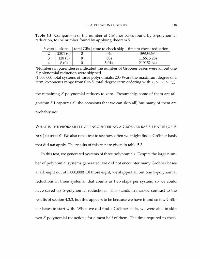
5.3. APPLICATION OF RESULT 118
Table 5.3: Comparison of the number of Gröbner bases found by S-polynomialreduction, to the number found by applying theorem 5.1.
# vars skips total GBs time to check skip time to check reduction2 2301 (0) 0 .04s 39803.68s3 128 (3) 8 .08s 116615.28s4 8 (0) 0 5.01s 219152.64s
*Numbers in parentheses indicated the number of Gröbner bases were all but oneS-polynomial reduction were skipped.(1,000,000 total systems of three polynomials; 20×#vars the maximum degree of aterm; exponents range from 0 to 5; total-degree term ordering with x1 � · · · � xn)
the remaining S-polynomial reduces to zero. Presumably, some of them are (al-
gorithm 5.1 captures all the occasions that we can skip all) but many of them are
probably not.
WHAT IS THE PROBABILITY OF ENCOUNTERING A GRÖBNER BASIS THAT IS (OR IS
NOT) SKIPPED? We also ran a test to see how often we might find a Gröbner basis
that did not apply. The results of this test are given in table 5.3.
In this test, we generated systems of three polynomials. Despite the large num-
ber of polynomial systems generated, we did not encounter many Gröbner bases
at all: eight out of 3,000,000! Of those eight, we skipped all but one S-polynomial
reductions in three systems: that counts as two skips per system, so we could
have saved six S-polynomial reductions. This stands in marked contrast to the
results of section 4.3.3, but this appears to be because we have found so few Gröb-
ner bases to start with. When we did find a Gröbner basis, we were able to skip
two S-polynomial reductions for almost half of them. The time required to check

5.3. APPLICATION OF RESULT 119
whether we can skip all but one S-polynomial remains quite small in comparison
to the time required to check the system by S-polynomial reduction.
Chapter 6
Skipping all but two S-polynomial
reductions (case for three polynomials)
6.1. PROBLEM
After chapters 4 and 5, the next logical step is to find a criterion for skipping all
but two S-polynomial reductions. Formally, we want an algorithm that decides
CC (t1, . . . , tm,�, {(1, 2) , (2, 3)})
We first approached this problem in the same manner as in the previous two chap-
ters: we tried to build counterexamples to show that Buchberger’s two criteria
were the best that we could do, as in theorems 4.1 on page 87 and 5.1 on page 102.
This turned out to be much more difficult than we anticipated. We have yet to find
the solution to this general form for m terms.
120

6.1. PROBLEM 121
We decided to restrict the problem to a more specific form:
CC (t1, t2, t3,�, {(1, 2) , (2, 3)})
By definition 3.1 on page 80, this is equivalent to[S1,2
∗−→(f1,f2,f3)
0 and S2,3∗−→
(f1,f2,f3)0 ⇒ S1,3
∗−→(f1,f2,f3)
0
]∀f1, f2, f3 such that fk = tk
At first, this also turned out to be too difficult (but we will return to it before long).
At this point, we restricted term ordering:
CC (t1, t2, t3, lex (x0, x1, x2, x3) , {(1, 2) , (2, 3)})
Again, the problem turned out to be too difficult. We were able to show that Buch-
berger’s criteria were necessary for most cases, but the last case resisted solution.
In this case, the leading terms satisfied
(6.1) gcd (t1, t3) | t2
One day, we sat down at the computer and used Maple to trace through all possible
reductions for all polynomials with these leading terms:
t1 = x0x1 t2 = x0x2 t3 = x0x3

6.1. PROBLEM 122
Notice that gcd (t1, t3) = x0 and t2 = x0x2, so these leading terms satisfy (6.1).
On the other hand, no permutation of the terms gives either gcd (t1, t3) = 1 or
t2 | lcm (t1, t3), so Buchberger’s criteria do not apply to these terms.
When we say that we used Maple to trace through “all polynomials with these
leading terms,” we mean with respect to lex (x0, x1, x2, x3), as indicated above. This
gives the form
fk = t0tk + t0 · A + B
where, for all monomials m in A or in B, t0 - m.
To our amazement, we learned that in this restricted situation,
S1,2∗−→
(f1,f2,f3)0 and S2,3
∗−→(f1,f2,f3)
0 ⇒ S1,3∗−→
(f1,f2,f3)0
This means that Buchberger’s criteria are not the only combinatorial criteria that
allow us to skip S-polynomial reduction.
After writing, correcting, and revising the proof, we generalized it to the form
t1 = x0xα11 t2 = x0x
α22 t3 = x0x
α33
The restriction that �= lex (x0, x1, x2, x3) remained. We tried to remove this condi-
tion, but we hit another brick wall; several months would pass before we finally
found a criterion independent of the term ordering. We present it in theorem 6.3.
6.2. RESULT 123
6.2. RESULT
We need to define two new combinatorial criteria.
DEFINITION 6.1. For all indeterminates x, we write
VB1x (t1, t3)⇔ min (degx t1, degx t3) = 0
VB2x (t1, t2, t3)⇔ degx t2 ≤ max (degx t1, degx t3)
We can consider these two criteria “variable-wise Buchberger criteria”: the first
is satisfied if t1 and t3 are relatively prime with respect to x (but not necessarily
with respect to all variables); the second is satisfied if t2 divides the least common
multiple of t1 and t3 on x (but not necessarily on all variables).
The following example will help familiarize us with the criteria.
EXAMPLE 6.2. Let
t1 = x0x1 t2 = x0x2 t3 = x0x3
Observe that degx0t2 = degx0
t1, so
VB2x0 (t1, t2, t3)
Also, for k = 1, 2, 3 we have at least one of degxkt1 = 0 or degxk
t3 = 0, so
VB1xk(t1, t3)
Hence one of the “variable-wise” criteria applies to each indeterminate. �

6.2. RESULT 124
Our main theorem is
THEOREM 6.3. (A)⇔ (B) where
(A) [ S1,2∗−→
(f1,f2,f3)0 and S2,3
∗−→(f1,f2,f3)
0 ] implies S1,3 0
∀f1, f2, f3 such that fk = tk
(B) (B1) or (B2) where
(B1) gcd (t1, t3) | t2 or BC2 (t1, t2, t3)
(B2) VB1x (t1, t3) or VB2x (t1, t2, t3) ∀x ∈ {x1, . . . , xm}
We can consider (B) to have two parts: a divisibility criterion (B1), and a variable-
wise Buchberger criterion (B2). Notice that theorem 6.3 provides criteria for the
second complete criterion mentioned in the introduction, not the first. We repeat
that the first complete criterion remains open for m > 3.
Observe that if Buchberger’s criteria are satisfied, then (B) is also satisfied.
Why? Assume first that BC1 (t1, t3). Then gcd (t1, t3) = 1; (B1) is satisfied by
gcd (t1, t3) | t2, and (B2) is satisfied by ∀x VB1x (t1, t3). On the other hand, sup-
pose that we have instead BC2 (t1, t2, t3). Then t2 | lcm (t1, t3); (B1) is satisfied by
BC2 (t1, t2, t3), and (B2) is satisfied by ∀x VB2x (t1, t2, t3). (See also lemma 6.19 on
page 166 below.)
Note also that if some tk = 1, (B) is also satisfied: one of the divisibility condi-
tions of (B1) is trivial; as is one of the variable-wise Buchberger criteria of (B2).
The proof of theorem 6.3 is long; we present it in three sections:

6.2. RESULT 125
• useful facts (section 6.2.1)
• proof that (B) is necessary to (A) (section 6.2.2)
• proof that (B) is sufficient for (A) (section 6.2.3)
Let’s consider one last example that will show how we discovered the criterion
and its proof.
EXAMPLE 6.4. Let �= lex (x, y, z) and
f1 = y6z2 + z4 + xz3 f2 = x2z6 + xy6z5 + x4y4z f3 = z3 + y6z
We have
f1 = xz3 f2 = x4y4z f3 = y6z
The criteria of theorem 6.3 are satisfied; the divisibility criterion because
gcd(f1 , f3
)= z f2 = x4y4z
and the variable-wise Buchberger criteria because
VB1x (t1, t3)
VB1y (t1, t3)
VB2z (t1, t2, t3)
We want to see why we can skip the reduction of S1,3. First we compute it:
S1,3 =xy6z3
xz3·(y6z2 + z4 + xz3
)− xy6z3
y6z·(z3 + y6z
)

6.2. RESULT 126
= y12z2 + y6z4 − xz5
How does this reduce?
S1,3 −→−z2·f1
y12z2 + 2y6z4 + z6
−→y6z·f3
y6z4 + z6
−→z3·f3
0
Collecting the quotients, we have the representation
S1,3 = h1f1 + h3f3
where
h1 = −z2 h3 = y6z + z3
Where do these polynomials come from? Look again at f1, f3. They have a greatest
common divisor. Separating it from its cofactors, we have
f1 = z(y6z + z3 + xz2
)f2 = z
(z2 + y6
)The non-leading monomials of the cofactors are
y6z + z3 z2
These cofactors look suspiciously similar to h1, h3! �
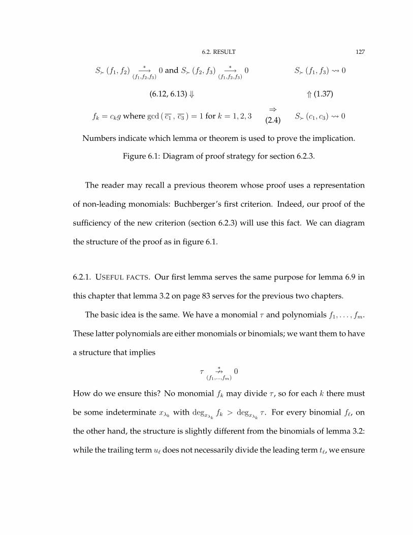
6.2. RESULT 127
S� (f1, f2)∗−→
(f1,f2,f3)0 and S� (f2, f3)
∗−→(f1,f2,f3)
0 S� (f1, f3) 0
(6.12, 6.13) ⇓ ⇑ (1.37)
fk = ckg where gcd ( c1 , c3 ) = 1 for k = 1, 2, 3⇒
(2.4) S� (c1, c3) 0
Numbers indicate which lemma or theorem is used to prove the implication.
Figure 6.1: Diagram of proof strategy for section 6.2.3.
The reader may recall a previous theorem whose proof uses a representation
of non-leading monomials: Buchberger’s first criterion. Indeed, our proof of the
sufficiency of the new criterion (section 6.2.3) will use this fact. We can diagram
the structure of the proof as in figure 6.1.
6.2.1. USEFUL FACTS. Our first lemma serves the same purpose for lemma 6.9 in
this chapter that lemma 3.2 on page 83 serves for the previous two chapters.
The basic idea is the same. We have a monomial τ and polynomials f1, . . . , fm.
These latter polynomials are either monomials or binomials; we want them to have
a structure that implies
τ∗9
(f1,...,fm)0
How do we ensure this? No monomial fk may divide τ , so for each k there must
be some indeterminate xλkwith degxλk
fk > degxλkτ . For every binomial f`, on
the other hand, the structure is slightly different from the binomials of lemma 3.2:
while the trailing term u` does not necessarily divide the leading term t`, we ensure

6.2. RESULT 128
that for each xλknoted for the monomials fk, degxλk
u` < degxλkt`. That way, τ −→
fk
τ ′ preserves degxλkfk > degxλk
τ ′.
LEMMA 6.5. Let τ be a nonzero monomial, and F = (f1, . . . , fm) a system of polynomials.
Then (A)⇒(B) where
(A) ∃µ with 1 ≤ µ ≤ m and ∃λ1, . . . , λµ such that [ (A1) and (A2) ] where
(A1) ∀` = 1, . . . , µ such that
degxλ`f` > degxλ`
τ
(A2) ∀` = µ + 1, . . . ,m
f` = t` + u`
t` � u`
degxλit` ≥ degxλi
u` ∀i = 1, . . . , µ
(B) τ∗9F
0.
PROOF. Assume (A). We want to show (B).
Consider an arbitrary reduction path of τ over F :
τ = τ0 −→fk1
τ1 −→fk2
· · · −→fkr
τr 9F
We want to show τr 6= 0. We show this by proving that τi and f1, . . . , fm satisfy
(A) for i = 1, . . . , r − 1; since τi can reduce only over a binomial, τi+1 6= 0. We
proceed by induction on i.
Inductive base: i = 0

6.2. RESULT 129
Since τ0 = τ , we know by hypothesis that τ0 and f1, . . . , fm satisfy (A).
Inductive step:
Assume that τi 6= 0, and that τi and f1, . . . , fm satisfy (A).
We show that τi+1 6= 0, and that τi+1 and f1, . . . , fm also satisfy (A).
Let ` be such that τi −→f`
τi+1.
Since τi satisfies (A1), we know that fk - τi for k = 1, . . . , µ.
Thus ` > µ, so τi+1 6= 0.
Let k ∈ {1, . . . , µ} be arbitrary, but fixed.
Again, τi satisfies (A1), so ∃λk such that
degxλkfk > degxλk
τi
Then
degxλkτi+1 = degxλk
(τi
t`· u`
)≤ degxλk
(τi
t`· t`)
= degxλkτi
Hence
degxλkfk > degxλk
τi+1
Since k was arbitrary, τi+1 and f1, . . . , fM satisfy (A).
Thus every monomial τi in the reduction path is nonzero; in particular, τr 6= 0
and τ∗9F
0. �

6.2. RESULT 130
The second lemma will also be useful for constructing a counterexample in
lemma 6.9.
LEMMA 6.6. The following are equivalent for all terms t1, t2, t3:
(A) gcd (t1, t3) | t2
(B) gcd (t1, t3) | gcd (t1, t2)
(C) gcd (t1, t3) | gcd (t2, t3)
PROOF. Let t1, t2, t3 be arbitrary, but fixed.
(A)⇒(B): Assume gcd (t1, t3) | t2. Equivalently,
∀x min (degx t1, degx t3) ≤ degx t2.
If degx t1 > degx t2, then degx t3 ≤ degx t2; hence gcd (t1, t3) | gcd (t1, t2).
(A)⇐(B): Assume gcd (t1, t3) | gcd (t1, t2). Equivalently,
∀x min (degx t1, degx t3) ≤ min (degx t1, degx t2) .
If degx t1 > degx t2, then degx t3 ≤ degx t2. Thus gcd (t1, t3) | t2.
(A)⇒(C) is symmetric to (A)⇒(B), exchanging t1 and t3.
(A)⇐(C) is symmetric to (A)⇐(B), exchanging t1 and t3. �
REMARK 6.7. For any term ordering � and for any two polynomials fi, fj , if g | fi
and g | fj , it follows from lemma 1.13 on page 15 that g | fi and g | fj . So if fi
and fj are relatively prime, fi and fj have no nontrivial common factors.
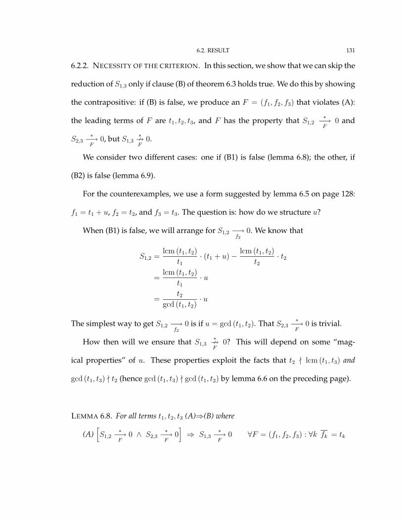
6.2. RESULT 131
6.2.2. NECESSITY OF THE CRITERION. In this section, we show that we can skip the
reduction of S1,3 only if clause (B) of theorem 6.3 holds true. We do this by showing
the contrapositive: if (B) is false, we produce an F = (f1, f2, f3) that violates (A):
the leading terms of F are t1, t2, t3, and F has the property that S1,2∗−→F
0 and
S2,3∗−→F
0, but S1,3∗9F
0.
We consider two different cases: one if (B1) is false (lemma 6.8); the other, if
(B2) is false (lemma 6.9).
For the counterexamples, we use a form suggested by lemma 6.5 on page 128:
f1 = t1 + u, f2 = t2, and f3 = t3. The question is: how do we structure u?
When (B1) is false, we will arrange for S1,2 −→f2
0. We know that
S1,2 =lcm (t1, t2)
t1· (t1 + u)− lcm (t1, t2)
t2· t2
=lcm (t1, t2)
t1· u
=t2
gcd (t1, t2)· u
The simplest way to get S1,2 −→f2
0 is if u = gcd (t1, t2). That S2,3∗−→F
0 is trivial.
How then will we ensure that S1,3∗9F
0? This will depend on some “mag-
ical properties” of u. These properties exploit the facts that t2 - lcm (t1, t3) and
gcd (t1, t3) - t2 (hence gcd (t1, t3) - gcd (t1, t2) by lemma 6.6 on the preceding page).
LEMMA 6.8. For all terms t1, t2, t3 (A)⇒(B) where
(A)[S1,2
∗−→F
0 ∧ S2,3∗−→F
0]⇒ S1,3
∗−→F
0 ∀F = (f1, f2, f3) : ∀k fk = tk

6.2. RESULT 132
(B) gcd (t1, t3) | t2 or BC2 (t1, t2, t3)
In the proof of lemma 6.8, we do not need the general machinery of lemma 6.5,
so we use the simpler form of lemma 3.2 on page 83.
PROOF. We show (A)⇒(B) by proving its contrapositive.
Assume ¬(B): gcd (t1, t3) - t2 and ¬BC2 (t1, t2, t3). We construct F to show ¬(A):
let F = (f1, f2, f3) be such that
f1 = t1 + gcd (t1, t2)
f2 = t2
f3 = t3
We need to show that f1 is a binomial, and f1 = t1.
Since gcd (t1, t2) | t1, we have gcd (t1, t2) � t1.
It remains to show that gcd (t1, t2) 6= t1. By way of contradiction:
gcd (t1, t2) = t1 ⇒ t1 | t2 ⇒ gcd (t1, t3) | t2
But ¬(A) has gcd (t1, t3) - t2.
So gcd (t1, t2) 6= t1.
Hence gcd (t1, t2) ≺ t1.
Hence f1 is a binomial, and f1 = t1.
We claim S1,2∗−→F
0 and S2,3∗−→F
0 but S1,3∗9F
0.

6.2. RESULT 133
From the construction of F
S2,3 = 0
Also
S1,2 =lcm (t1, t2)
t1· (t1 + u)− lcm (t1, t2)
t2· t2
=t2
gcd (t1, t2)· gcd (t1, t2)
= f2
So S1,2∗−→F
0 and S2,3∗−→F
0.
Consider
S1,3 =lcm (t1, t3)
t1· (t1 + u)− lcm (t1, t3)
t3· t3
=t3
gcd (t1, t3)· u
We claim that t2 - S1,3.
Assume by way of contradiction that t2 | S13.
Then
t2 |t3
gcd (t1, t3)· gcd (t1, t2)
This implies that
t2 |t3
gcd (t1, t3)· t1
Then t2 | lcm (t1, t3).
This contradicts t2 - lcm (t1, t3).

6.2. RESULT 134
Hence t2 - S1,3.
We further claim that t3 - S1,3.
Assume by way of contradiction that t3 | S1,3.
Then gcd (t1, t3) | u.
Since u = gcd (t1, t2), we have gcd (t1, t3) | gcd (t1, t2).
By lemma 6.6 on page 130, gcd (t1, t3) | t2.
This contradicts gcd (t1, t3) - t2.
Hence t3 - S1,3.
By lemma 3.2, S1,3∗9F
0. (Use the permutation (1 3 2) with µ = 1.) �
For clause (B2) in theorem 6.3, we employ a similar approach. As before, we
build F = (f1, f2, f3) “as simple as possible”: f2 and f3 will be monomials, and
f1 = t1 + u where u will have the “magical properties” that S1,2 −→F
0 but S1,3∗9F
0.
We find the “magical properties” by exploiting the failure of the criterion: in this
case, the existence of an indeterminate y ∈ {x1, . . . , xm} such that ¬VB1y (t1, t3)
and ¬VB2y (t1, t2, t3). More precisely, we exploit degy σ12 > degy σ13: a sufficiently
small choice for degy u gives S1,2∗−→f3
0 while S1,3∗9F
0, since
degy S1,2 = degy (σ12u) > degy (σ13u) = degy S1,3
In this proof, we use the full generality of lemma 6.5 on page 128.
LEMMA 6.9. For all terms t1, t2, t3, (A)⇒(B) where

6.2. RESULT 135
(A)[S1,2
∗−→F
0 ∧ S2,3∗−→F
0]⇒ S1,3
∗−→F
0 ∀F = (f1, f2, f3) : ∀k fk = tk
(B) VB1x (t1, t3) or VB2x (t1, t2, t3) ∀x ∈ {x1, . . . , xn}
PROOF. We show (A)⇒(B) by proving its contrapositive.
Assume ¬(B); then ∃y ∈ {x1, . . . , xn} such that
¬VB1y (t1, t3) and ¬VB2y (t1, t2, t3)
Equivalently, ∃y such that
0 < degy t1, degy t3 < degy t2
We need to find F such that S1,2∗−→F
0 and S2,3∗−→F
0 but S1,3∗9F
0.
Without loss of generality, we may assume degy t1 ≤ degy t3. If not, swap t1 and
t3 for the remainder of the proof.
Case 1: t1 � t3
Define u as
∀x ∈ {x1, . . . , xn} degx u =
degx t3 x 6= y
max(0, degy t1 + degy t3 − degy t2
)x = y
Let F = (f1, f2, f3) be such that
f1 = t1 + u
f2 = t2
f3 = t3

6.2. RESULT 136
Note that u | t3 and u 6= t3; hence u ≺ t3 � t1. Hence f1 is a binomial with
f1 = t1.
We claim that S1,2∗−→F
0 and S2,3∗−→F
0 but S1,3∗9F
0.
Immediately we have S2,3 = 0, so S2,3∗−→
(f1,f2,f3)0 trivially.
Next,
S1,2 =lcm (t1, t2)
t1· (t1 + u)− lcm (t1, t2)
t2· t2
= lcm (t1, t2) +lcm (t1, t2)
t1· u− lcm (t1, t2)
=lcm (t1, t2)
t1· u
We see that for x 6= y
degx S1,2 = max (degx t1, degx t2)− degx t1 + degx u
≥ degx u
= degx t3
whereas
degy S1,2 = max(degy t1, degy t2
)− degy t1 + max
(0, degy t1 + degy t3 − degy t2
)Recall degy t2 > degy t1. Then
degy S1,2 = degy t2 − degy t1 + max(0, degy t1 + degy t3 − degy t2
)= max
(degy t2 − degy t1, degy t3
)

6.2. RESULT 137
≥ degy t3
So S1,2∗−→f3
0, as desired.
Now we turn to S1,3. By reasoning similar to that for S1,2, we have
S1,3 =lcm (t1, t3)
t1· u
We claim degy S1,3 < degy t3 < degy t2.
We have
degy S1,3 = max(degy t1, degy t3
)− degy t1 + max
(0, degy t1 + degy t3 − degy t2
)Recall degy t1 ≤ degy t3.
Then
degy S1,3 = degy t3 − degy t1 + max(0, degy t1 + degy t3 − degy t2
)= max
(degy t3 − degy t1, 2 degy t3 − degy t2
)Recall degy t3 < degy t2 and 0 < degy t1.
Then
degy S1,3 < degy t3 < degy t2
Recall degy t1 ≥ degy t3 > degy u.
By lemma 6.5, S1,3∗9F
0.
Case 2: t1 ≺ t3
We sketch the proof; it is similar to that for case 1.
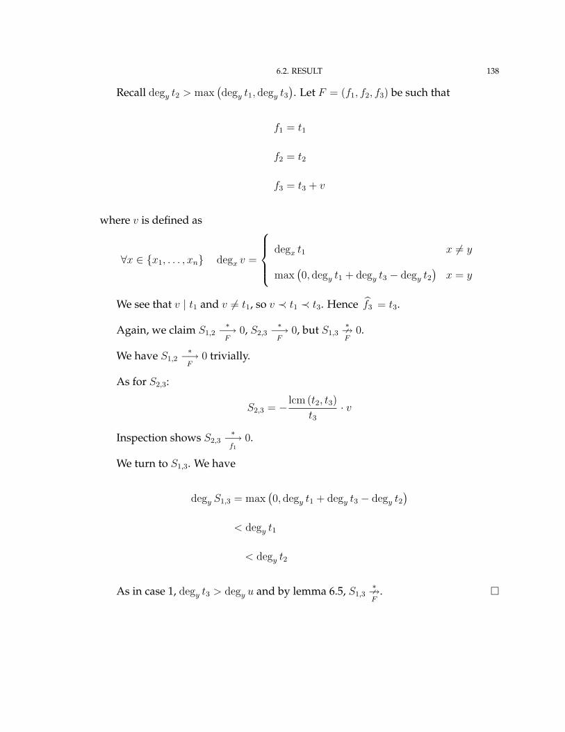
6.2. RESULT 138
Recall degy t2 > max(degy t1, degy t3
). Let F = (f1, f2, f3) be such that
f1 = t1
f2 = t2
f3 = t3 + v
where v is defined as
∀x ∈ {x1, . . . , xn} degx v =
degx t1 x 6= y
max(0, degy t1 + degy t3 − degy t2
)x = y
We see that v | t1 and v 6= t1, so v ≺ t1 ≺ t3. Hence f3 = t3.
Again, we claim S1,2∗−→F
0, S2,3∗−→F
0, but S1,3∗9F
0.
We have S1,2∗−→F
0 trivially.
As for S2,3:
S2,3 = − lcm (t2, t3)
t3· v
Inspection shows S2,3∗−→f1
0.
We turn to S1,3. We have
degy S1,3 = max(0, degy t1 + degy t3 − degy t2
)< degy t1
< degy t2
As in case 1, degy t3 > degy u and by lemma 6.5, S1,3∗9F
. �

6.2. RESULT 139
In lemmas 6.8 and 6.9, we have proven the following strict boundary on triplets
of terms that guarantee S13 0.
COROLLARY 6.10. For all terms t1, t2, t3 (A)⇒(B) where
(A)[S12
∗−→F
0 ∧ S23∗−→F
0]⇒ S13
∗−→F
0 ∀F = (f1, f2, f3) : ∀k fk = tk
(B) clause (B) of theorem 6.3
6.2.3. SUFFICIENCY OF THE CRITERION. We turn our attention to proving that the
new combinatorial criterion of theorem 6.3 eliminates the need to check the reduc-
tion of an S-polynomial. This is the more complicated part of the proof of theorem
6.3; the reader may wish to review figure 6.1 on page 127.
We need the following observation. Note the subtle difference between remark
6.11, which is true only if gcd (t1, t3) | t2, and remark 1.35 on page 49, which is true
in all cases.
LEMMA 6.11. If gcd (t1, t3) | t2, then gcd ( σ21 , σ23 ) = 1 for all fk = tk.
PROOF. Let t1, t2, t3 be arbitrary, but fixed. Assume gcd (t1, t3) | t2. Then ∀x
min (degx t1, degx t3) ≤ degx t2
Assume ∃y such that y | σ23 . We have
degy σ23 = degy
lcm(f2 , f3
)f2
= max(degy t2, degy t3
)− degy t2

6.2. RESULT 140
= max(0, degy t3 − degy t2
)Since y | σ23 , degy t3 > degy t2.
Recall min(degy t1, degy t3
)≤ degy t2; with the above, this implies degy t1 ≤
degy t2. Hence
degy σ21 = degy
lcm(f1 , f2
)f2
= max(degy t1, degy t2
)− degy t2 = 0 �
We come to the meat of the proof. We proceed by factoring the common divisor
of f1, f3. Lemma 6.12 shows that when the new criterion is satisfied and the two
“chain” S-polynomials reduce, we have a surprising result: gcd (f1, f3) | f2.
LEMMA 6.12. (A)⇐(B) where
(A) S1,2∗−→F
0 and S2,3∗−→F
0 implies g13 | f2 where g13 = gcd (f1, f3),
(B) gcd(f1 , f3
)| f2
PROOF. Assume (B). Then gcd(f1 , f3
)| f2 .
Assume S1,2∗−→F
0 and S2,3∗−→F
0. We need to show g13 | f2.
Apply S1,2∗−→F
0 and lemma 1.28 on page 30 to obtain a representation h1, h2, h3
of S1,2. So
(6.2) S1,2 = h1f1 + h2f2 + h3f3
and ∀k = 1, 2, 3, hk 6= 0 implies hkfk ≺ lcm(f1 , f2
).

6.2. RESULT 141
Likewise, from S2,3∗−→F
0 obtain a representation H1, H2, H3, so that
(6.3) S2,3 = H1f1 + H2f2 + H3f3
and ∀k = 1, 2, 3, Hk 6= 0 implies Hkfk ≺ lcm(f2 , f3
).
Consider (6.2). We have
σ12f1 − σ21f2 = h1f1 + h2f2 + h3f3
(σ12 − h1) f1 − h3f3 = (σ21 + h2) f2(6.4)
Likewise (6.3) gives us
(6.5) H1f1 + (σ32 + H3) f3 = (σ23 −H2) f2
Let g13 = gcd (f1, f3).
Let c1, c3 be such that f1 = c1g13 and f3 = c3g13.
From (6.4), we have
(6.6) g13 [(σ12 − h1) c1 − h3c3] = (σ21 + h2) f2
From (6.5), we have
(6.7) g13 [H1c1 + (σ32 −H3) c3] = (σ23 −H2) f2
Note g13 | (σ21 + h2) f2 and g13 | (σ23 −H2) f2.
So g13 divides the greatest common divisor of (σ21 + h2) f2 and (σ23 −H2) f2.
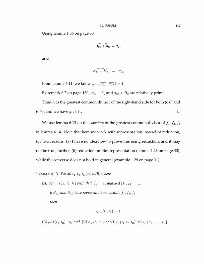
6.2. RESULT 142
Using lemma 1.36 on page 50,
σ21 + h2 = σ21
and
σ23 −H2 = σ23
From lemma 6.11, we know gcd ( σ21 , σ23 ) = 1.
By remark 6.7 on page 130 , σ21 + h2 and σ23 + H2 are relatively prime.
Thus f2 is the greatest common divisor of the right-hand side for both (6.6) and
(6.7), and we have g13 | f2. �
We use lemma 6.13 on the cofactors of the greatest common divisor of f1, f2, f3
in lemma 6.14. Note that here we work with representation instead of reduction,
for two reasons: (a) I have no idea how to prove this using reduction, and it may
not be true; further, (b) reduction implies representation (lemma 1.28 on page 30),
while the converse does not hold in general (example 1.29 on page 31).
LEMMA 6.13. For all t1, t2, t3 (A)⇐(B) where
(A) ∀F = (f1, f2, f3) such that fk = tk and gcd (f1, f3) = 1,
if S1,2 and S2,3 have representations modulo f1, f2, f3
then
gcd (t1, t3) = 1
(B) gcd (t1, t3) | t2 and [VB1x (t1, t3) or VB2x (t1, t2, t3)] ∀x ∈ {x1, . . . , xn}

6.2. RESULT 143
PROOF. Assume (B).
Let F be arbitrary but fixed.
Assume S1,2 and S2,3 have representations modulo f1, f2, f3. Choose h1, h2, h3
such that
(6.8) S1,2 = h1f1 + h2f2 + h3f3 and ∀k hk 6= 0⇒ hk · fk ≺ lcm(f1 , f2
)and H1, H2, H3 such that
(6.9) S2,3 = H1f1 + H2f2 + H3f3 and ∀k Hk 6= 0⇒ Hk · fk ≺ lcm(f2 , f3
)From (6.8),
σ12f1 − σ21f2 = h1f1 + h2f2 + h3f3
(σ12 − h1) f1 − h3f3 = (σ21 + h2) f2
(σ12 − h1) f1 − h3f3
σ21 + h2
= f2(6.10)
Likewise from (6.9),
(6.11)H1f1 + (σ32 + H3) f3
σ23 −H2
= f2
From (6.10) and (6.11),
(σ12 − h1) f1 − h3f3
σ21 + h2
=H1f1 + (σ32 + H3) f3
σ23 −H2
(σ23 −H2) [(σ12 − h1) f1 − h3f3] = (σ21 + h2) [H1f1 + (σ32 + H3) f3]
6.2. RESULT 144
Collect expressions with f1 and f3 on opposite sides:
(6.12)
[(σ23 −H2) (σ12 − h1)−H1 (σ21 + h2)] f1 = [h3 (σ23 −H2) + (σ21 + h2) (σ32 + H3)] f3
Let
P = h3 (σ23 −H2) + (σ21 + h2) (σ32 + H3)
Note that P is the cofactor of f1 in (6.12).
We claim P = σ21 · σ32.
As per lemma 1.36,
• σ23 � H2
• σ21 � h2
• σ32 � H3
So the only possible leading monomials of P are σ21 · σ32 and σ23 · h3 .
Assume by way of contradiction that
σ23 · h3 � σ21 · σ32
Then
lcm(f2 , f3
)f2
· h3 �lcm
(f1 , f2
)f2
·lcm
(f2 , f3
)f3
Canceling, we find that this implies
h3 �lcm
(f1 , f2
)f3
6.2. RESULT 145
f3 · h3 � lcm(f1 , f2
)This clearly contradicts (6.8).
Hence P = σ21 · σ32.
Observe that f1 divides the left-hand side of (6.12). So f1 must also divide the
right-hand side of (6.12).
Recall that f1 and f3 are relatively prime. Thus
f1 | P
Then f1 | P . That is,
t1 | σ21 · σ32
t1 |lcm
(f1 , f2
)f2
·lcm
(f2 , f3
)f3
t1 |lcm (t1, t2)
t2· lcm (t2, t3)
t3
t1 |t1t2
gcd (t1, t2) · t2· t2t3gcd (t2, t3) · t3
gcd (t1, t2) · gcd (t2, t3) | t2(6.13)
We claim this proves gcd (t1, t3) = 1. Why?
Let x be an arbitrary, but fixed indeterminate.
Recall from (B) that:
gcd (t1, t3) | t2, and
for all x VB1x (t1, t3) or VB2x (t1, t2, t3).

6.2. RESULT 146
It will suffice to show that VB2x (t1, t2, t3) and (6.13) imply VB1x (t1, t3).
Assume VB2x (t1, t2, t3).
Suppose degx t1 ≤ degx t3
From (B), degx t1 ≤ degx t2 ≤ degx t3.
From (6.13),
degx t1 + degx t2 ≤ degx t2
So degx t1 = 0.
Hence VB1x (t1, t3).
If instead degx t1 > degx t3, a similar argument gives VB1x (t1, t3).
Hence VB2x (t1, t2, t3) and (6.13) imply VB1x (t1, t3).
Since x was arbitrary, degx t1 = 0 or degx t3 = 0, for all indeterminates x.
Thus gcd (t1, t3) = 1. �
Lemma 6.14 completes the proof of the main theorem, by showing that the new
criterion suffices to skip the reduction of one S-polynomial. Because we switch
between two sets of polynomials (fk and ck), we maintain the long notation for
S-polynomials (S� (fi, fj) instead of Si,j).
LEMMA 6.14. For all terms t1, t2, t3 (A)⇐(B) where
(A)[S� (f1, f2)
∗−→F
0 and S� (f2, f3)∗−→F
0]⇒ S� (f1, f3) 0
∀F = (f1, f2, f3) such that fk = tk.
(B) clause (B) of theorem 6.3.

6.2. RESULT 147
PROOF. Assume (B). Thus we have (B1) and (B2) of theorem 6.3.
Let F be arbitrary, but fixed. Assume S1,2∗−→F
0 and S2,3∗−→F
0. We consider
two cases.
Case 1: BC2 (t1, t2, t3)
(A) follows from corollary 2.9 on page 69.
Case 2: ¬BC2 (t1, t2, t3)
From (B), we have
(6.14) gcd (t1, t3) | t2 and [VB1x (t1, t3) or VB2x (t1, t2, t3) ∀x ∈ {x1, . . . , xn}]
Let g = gcd (f1, f3). Let c1, c3 be such that fk = ckg. Then c1 and c3 are relatively
prime.
Recall S� (f1, f2)∗−→F
0 and S� (f2, f3)∗−→F
0. From lemma 6.12, g | f2.
Let c2 be such that f2 = c2g.
Since tk = fk = ckg = ck · g , (6.14) implies
gcd ( c1 , c3 ) | c2 ∧ ∀x [VB1x ( c1 , c3 ) ∨ VB2x ( c1 , c2 , c3 )]
Recall again S� (f1, f3) and S� (f2, f3)∗−→F
0. It follows from lemma 1.28 on
page 30 that S� (f1, f2) and S� (f2, f3) have representations modulo F . By lemma
1.37 on page 51, we know that S� (c1, c2) and S� (c2, c3) have representations mod-
ulo c1, c2, c3. By lemma 6.13, c1 and c3 are relatively prime.
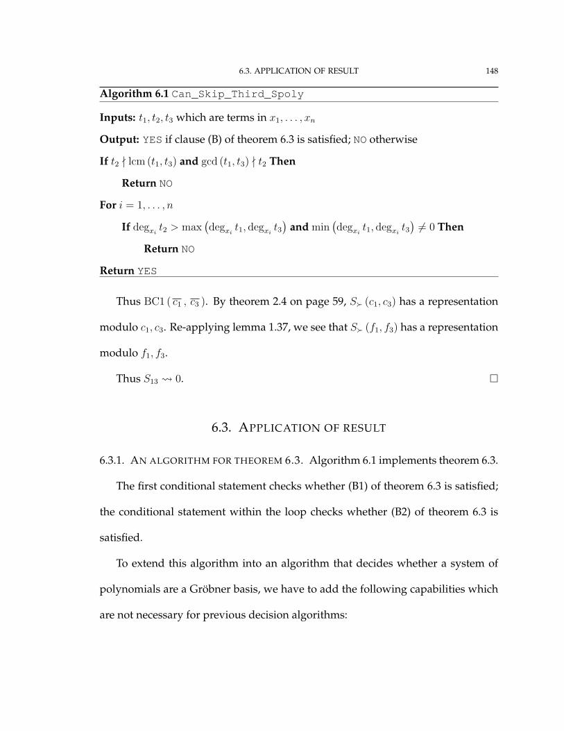
6.3. APPLICATION OF RESULT 148
Algorithm 6.1 Can_Skip_Third_Spoly
Inputs: t1, t2, t3 which are terms in x1, . . . , xn
Output: YESif clause (B) of theorem 6.3 is satisfied; NOotherwise
If t2 - lcm (t1, t3) and gcd (t1, t3) - t2 Then
Return NO
For i = 1, . . . , n
If degxit2 > max
(degxi
t1, degxit3)
and min(degxi
t1, degxit3)6= 0 Then
Return NO
Return YES
Thus BC1 ( c1 , c3 ). By theorem 2.4 on page 59, S� (c1, c3) has a representation
modulo c1, c3. Re-applying lemma 1.37, we see that S� (f1, f3) has a representation
modulo f1, f3.
Thus S13 0. �
6.3. APPLICATION OF RESULT
6.3.1. AN ALGORITHM FOR THEOREM 6.3. Algorithm 6.1 implements theorem 6.3.
The first conditional statement checks whether (B1) of theorem 6.3 is satisfied;
the conditional statement within the loop checks whether (B2) of theorem 6.3 is
satisfied.
To extend this algorithm into an algorithm that decides whether a system of
polynomials are a Gröbner basis, we have to add the following capabilities which
are not necessary for previous decision algorithms:

6.3. APPLICATION OF RESULT 149
• Remember the representation of each Si,j
• If Can_Skip_Third_SPoly returns YES for terms ti, tj, tk, en-
sure that the representations of Si,j and Sj,k are modulo fi, fj, fk
only
If Si,j or Sj,k reduces only over fi, fj, fk, then theorem 6.3 guarantees that we can
skip Si,k. Otherwise, we may not be able to skip Si,k: see example 6.18 below.
6.3.2. EXAMPLES OF THEOREM 6.3. Our first example will answer the question, Is
theorem 6.3 merely a rearrangement of Buchberger’s criteria, or does it contribute some-
thing new?
The theorem does contribute something new. We illustrate this with two exam-
ples. The first comes from our discussion at the beginning of this chapter.
EXAMPLE 6.15. Let t1 = x0x1, t2 = x0x2, and t3 = x0x3. Let � be any term ordering
whatsoever.
Observe that no arrangement of Buchberger’s criteria allows us to skip an S-
polynomial reduction:
• no pair ti, tj is relatively prime;
• no term tk can serve as a bridge, because no permutation of the
indices allows for tk | lcm (ti, tj)
6.3. APPLICATION OF RESULT 150
On the other hand, t1, t2, t3 do satisfy the combinatorial criterion of theorem 6.3.
Why? Clause (B1) is satisfied by gcd (t1, t3) = x0, and x0 | t2. Clause (B2) is satisfied
by
• VB2x0 (t1, t2, t3)
• VB1xk(t1, t3) for k = 1, 2, 3
Thus, we have a set of terms so that Buchberger’s criteria do not allow us to skip
an S-polynomial reduction, but theorem 6.3 does. In other words, theorem 6.3
provides a new combinatorial criterion for skipping S-polynomial reduction.
What is this new criterion? If we assume that both of Buchberger’s criteria fail,
then to skip an S-polynomial reduction, we must retain the following:
gcd (t1, t3) | t2
and
∀x VB1x (t1, t3) or VB2x (t1, t2, t3)
The next two examples use the term diagrams of section 2.5 to give us two-
dimensional and three-dimensional visualizations of what is new in the new cri-
terion. In each case, we pose the question: Given t1 and t3, what values of t2 give
S1,3 0, where the leading term of fk is tk? The reader may want to take a moment
to review term diagrams.
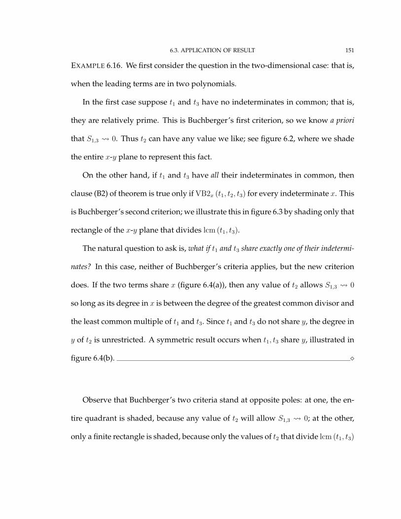
6.3. APPLICATION OF RESULT 151
EXAMPLE 6.16. We first consider the question in the two-dimensional case: that is,
when the leading terms are in two polynomials.
In the first case suppose t1 and t3 have no indeterminates in common; that is,
they are relatively prime. This is Buchberger’s first criterion, so we know a priori
that S1,3 0. Thus t2 can have any value we like; see figure 6.2, where we shade
the entire x-y plane to represent this fact.
On the other hand, if t1 and t3 have all their indeterminates in common, then
clause (B2) of theorem is true only if VB2x (t1, t2, t3) for every indeterminate x. This
is Buchberger’s second criterion; we illustrate this in figure 6.3 by shading only that
rectangle of the x-y plane that divides lcm (t1, t3).
The natural question to ask is, what if t1 and t3 share exactly one of their indetermi-
nates? In this case, neither of Buchberger’s criteria applies, but the new criterion
does. If the two terms share x (figure 6.4(a)), then any value of t2 allows S1,3 0
so long as its degree in x is between the degree of the greatest common divisor and
the least common multiple of t1 and t3. Since t1 and t3 do not share y, the degree in
y of t2 is unrestricted. A symmetric result occurs when t1, t3 share y, illustrated in
figure 6.4(b). �
Observe that Buchberger’s two criteria stand at opposite poles: at one, the en-
tire quadrant is shaded, because any value of t2 will allow S1,3 0; at the other,
only a finite rectangle is shaded, because only the values of t2 that divide lcm (t1, t3)

6.3. APPLICATION OF RESULT 152
0 3 521
y
5
4
x
3
2
1
04
-1
Term t2 can lie anywhere and S1,3 0.
Figure 6.2: Terms t1 and t3 have no indeterminates in common.
0
x-1
3
1
2
4
1
y
3
5
2
50
4
To guarantee S1,3 0, t2 can only lie in that region of the plane that divideslcm (t1, t3) (marked in blue).
Figure 6.3: Terms t1 and t3 have all their indeterminates in common.
allow S1,3 0. Between these two extremes, we have the case where the new cri-
terion applies, but neither of Buchberger’s criteria apply: t2 can lie anywhere in an
infinite region of the plane, but this region does not cover the entire plane.
We can observe this in the three-dimensional case as well.
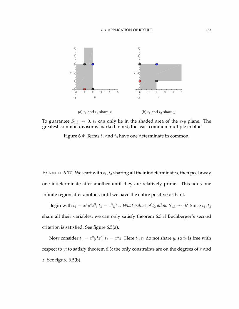
6.3. APPLICATION OF RESULT 153
54
1
2
4
-1
2
3100
3
5
x
y
(a) t1 and t3 share x
54
1
2
4
-1
2
3100
3
5
x
y
(b) t1 and t3 share y
To guarantee S1,3 0, t2 can only lie in the shaded area of the x-y plane. Thegreatest common divisor is marked in red; the least common multiple in blue.
Figure 6.4: Terms t1 and t3 have one determinate in common.
EXAMPLE 6.17. We start with t1, t3 sharing all their indeterminates, then peel away
one indeterminate after another until they are relatively prime. This adds one
infinite region after another, until we have the entire positive orthant.
Begin with t1 = x2y4z3, t3 = x5y2z. What values of t2 allow S1,3 0? Since t1, t3
share all their variables, we can only satisfy theorem 6.3 if Buchberger’s second
criterion is satisfied. See figure 6.5(a).
Now consider t1 = x2y4z3, t3 = x5z. Here t1, t3 do not share y, so t2 is free with
respect to y; to satisfy theorem 6.3; the only constraints are on the degrees of x and
z. See figure 6.5(b).
6.3. APPLICATION OF RESULT 154
In the next step, consider t1 = y4z3, t3 = x5z. In this case, t1, t3 only share z, so
t2 is free with respect to x and y; the only constraints are on the degree of z. See
figure 6.5(c).
Finally, let t1 = y4z3, t3 = x5. Now the two terms are relatively prime, so t2 is
free with respect to all indeterminates; we always have S1,3 0. We have arrived
at the pole of Buchberger’s first criterion; see figure 6.5(d). �
We close this section with an example that serves as a warning: the new crite-
rion does not extend in an obvious way to m > 3 leading terms. This is more subtle
than might first seem.
EXAMPLE 6.18. Let F = (f1, f2, f3, f4) where
f1 = x0x1 + x2 f2 = x0x2 f3 = x0x3 f4 = x22
Let � be any term ordering such that f1 = x0x1; for example, a total-degree
term ordering. Observe that f1 , f2 , f3 are the same as those of example 6.15;
hence, they satisfy (B) of theorem 6.3. However,
S1,2 = x22 −→
F0
S2,3 = 0
S1,3 = x2x3 9F
�
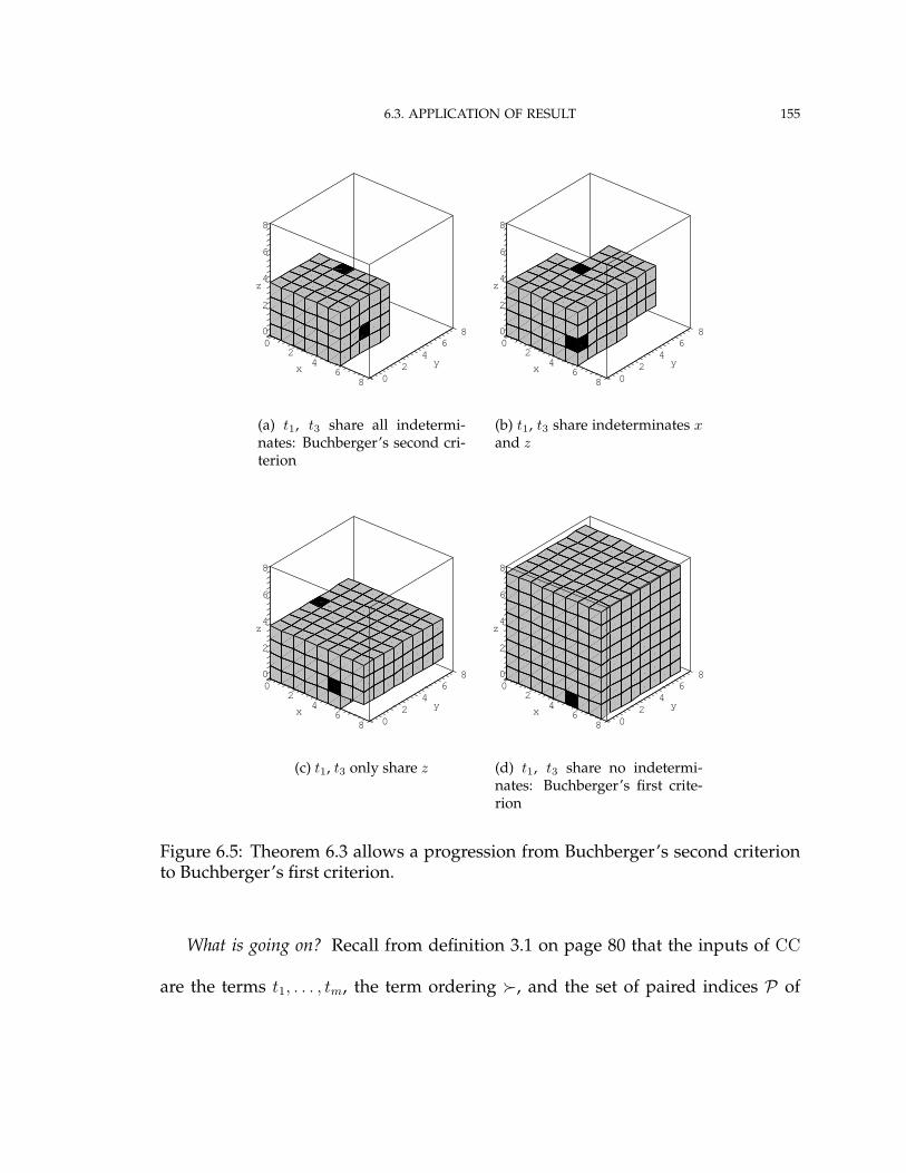
6.3. APPLICATION OF RESULT 155
800 6
2
2 4
4z
4 y2
6
x 6
8
08
(a) t1, t3 share all indetermi-nates: Buchberger’s second cri-terion
800 6
2
2 4
4z
4 y2
6
x 6
8
08
(b) t1, t3 share indeterminates xand z
800 6
2
2 4
4z
4 y2
6
x 6
8
08
(c) t1, t3 only share z
800 6
2
2 4
4z
4 y2
6
x 6
8
08
(d) t1, t3 share no indetermi-nates: Buchberger’s first crite-rion
Figure 6.5: Theorem 6.3 allows a progression from Buchberger’s second criterionto Buchberger’s first criterion.
What is going on? Recall from definition 3.1 on page 80 that the inputs of CC
are the terms t1, . . . , tm, the term ordering �, and the set of paired indices P of
6.3. APPLICATION OF RESULT 156
S-polynomials that are assumed to reduce to zero. The algorithm must decide[∀f1, . . . , fm such that fk = tk ∀ (i, j) ∈ P Si,j
∗−→(f1,...,fm)
0
]⇓
GB� (f1, . . . , fm)
Clause (A) of theorem 6.3 gives the inputs t1, t2, t3. This means that clause (B) is
necessary and sufficient for (A) only if
S1,2∗−→
(f1,f2,f3)0 and S2,3
∗−→(f1,f2,f3)
0
In other words, the S-polynomials must reduce only over the triplet f1, f2, f3 for the
new criterion to give us a valid skip. In example 6.18, the S-polynomial reduces
over a fourth polynomial; hence CC cannot guarantee that S1,3 will reduce to zero.
6.3.3. EXPERIMENTAL RESULTS. We ran experiments to answer two questions re-
garding these results:
• How often can we expect the new criterion to apply in real-life
situations?
• How often do S-polynomials reduce over r polynomials?
It should be obvious why we would pose the first question: although the restriction
on the number of polynomials means that the theorem is not “complete” enough
to expect very many occasions when we can skip one S-polynomial reduction, we
would still like an idea of how often the criterion might appear.
6.3. APPLICATION OF RESULT 157
The second question also tries to see how often the new criterion could appear,
but also whether further research would be useful. If we know how the majority of
S-polynomials reduce to zero during a Gröbner basis computation, and over what
number of polynomials they reduce to zero, this can help us design strategies for
faster Gröbner basis computation.
HOW OFTEN CAN WE EXPECT THE NEW CRITERION TO APPLY IN “REAL-LIFE” SIT-
UATIONS? In a first experiment suggested by Bruno Buchberger, we generated
three random terms t1, t2, t3, which we assumed to be the leading terms of un-
specified polynomials f1, f2, f3.
In a typical Buchberger algorithm for computing (or even deciding) Gröbner
bases, the critical pairs are ordered in some manner. For example, if t1 = x2y,
t2 = x3, and t3 = yz, using �= lex (x, y, z) we could order the critical pairs by
increasing least common multiple. Since
lcm (t2, t3) � lcm (t1, t2) � lcm (t1, t3)
the algorithm would first reduce S1,3, then S1,2, and finally S2,3.
After ordering the critical pairs, we assumed that the first two S-polynomials
reduce to zero. At this point, we checked which combinatorial criteria applied to
the leading terms. Since the terms that satisfy Buchberger’s criteria are a subset of
the terms that satisfy the new criterion, we checked them first. This gives us an
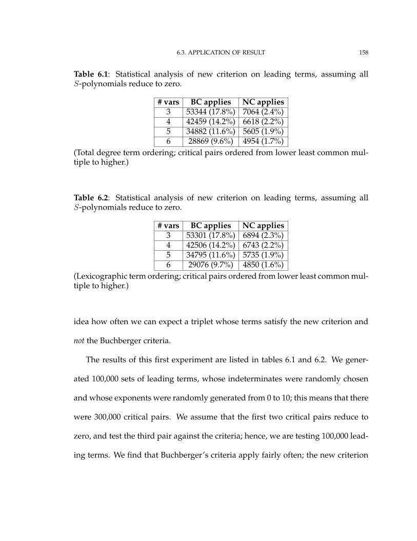
6.3. APPLICATION OF RESULT 158
Table 6.1: Statistical analysis of new criterion on leading terms, assuming allS-polynomials reduce to zero.
# vars BC applies NC applies3 53344 (17.8%) 7064 (2.4%)4 42459 (14.2%) 6618 (2.2%)5 34882 (11.6%) 5605 (1.9%)6 28869 (9.6%) 4954 (1.7%)
(Total degree term ordering; critical pairs ordered from lower least common mul-tiple to higher.)
Table 6.2: Statistical analysis of new criterion on leading terms, assuming allS-polynomials reduce to zero.
# vars BC applies NC applies3 53301 (17.8%) 6894 (2.3%)4 42506 (14.2%) 6743 (2.2%)5 34795 (11.6%) 5735 (1.9%)6 29076 (9.7%) 4850 (1.6%)
(Lexicographic term ordering; critical pairs ordered from lower least common mul-tiple to higher.)
idea how often we can expect a triplet whose terms satisfy the new criterion and
not the Buchberger criteria.
The results of this first experiment are listed in tables 6.1 and 6.2. We gener-
ated 100,000 sets of leading terms, whose indeterminates were randomly chosen
and whose exponents were randomly generated from 0 to 10; this means that there
were 300,000 critical pairs. We assume that the first two critical pairs reduce to
zero, and test the third pair against the criteria; hence, we are testing 100,000 lead-
ing terms. We find that Buchberger’s criteria apply fairly often; the new criterion

6.3. APPLICATION OF RESULT 159
appears rarely. The choice of term ordering does not appear to have a significant
effect on the results.
In another experiment suggested by Erich Kaltofen, we modified an algorithm
that computed Gröbner bases and ran it on randomly-generated polynomials as
well as some benchmark sets of polynomials. (See the footnote contrasting decid-
ing a Gröbner basis and computing a Gröbner basis on page 23.) The benchmarks
used were:
• Cyclic-3
• Cyclic-4
• Cyclic-5
• Katsura-5
The modifications were to keep detailed records of S-polynomial reduction. These
records are necessary for the correct implementation of the new criterion (which
requires that the S-polynomials reduce only over three polynomials). Both to en-
courage reduction to zero and to avoid expression swell and rational coefficients,
we carried out these computations over a field of characteristic two.
While Buchberger’s criteria occurred very frequently in the computation of
Gröbner bases for these benchmarks, the new criterion never appeared. In fact,
Buchberger’s criteria allow us to skip the majority of S-polynomial reductions.

6.3. APPLICATION OF RESULT 160
Table 6.3: Number of skips during the computation of a Gröbner basis for threerandomly-generated polynomials; total-degree term ordering.
Buchberger skips New skips Reductions Polys in GB1 16 1 (empty) 11 83 22 0 14 95 113 0 77 206 13 0 23 98 244 1 (empty) 133 28
10 22 4 (empty) 29 11
For randomly-generated polynomials, the results were a little more “positive”
(as in, non-zero). We give the results in table 6.3. Observe that with the excep-
tion of systems 6 and 10, Buchberger’s criteria allow us to skip the majority of S-
polynomial reductions. As for skips that are genuinely new criteria, we do see six to-
tal. However, they were all “empty” S-polynomials; that is, while the new criteria
would allow us to skip an S-polynomial reduction, the corresponding polynomi-
als were in fact monomials, so that no reduction would have taken place anyway.
(We note that these polynomials were generated with at least 2, at most 5 vari-
ables; at least 2, at most 5 terms; exponents ranged from 0 to 10, with total degree
5; coefficients ranged from -99 to 99.)
WHY SO RARE? The results of tables 6.1, 6.2 and 6.3 seem counter-intuitive to the
infinite regions of additional bridge terms afforded by the new criterion, as illus-
trated by figures 6.4 and 6.5. The question arises: why does the new criterion
appear so rarely? We can think of three reasons.
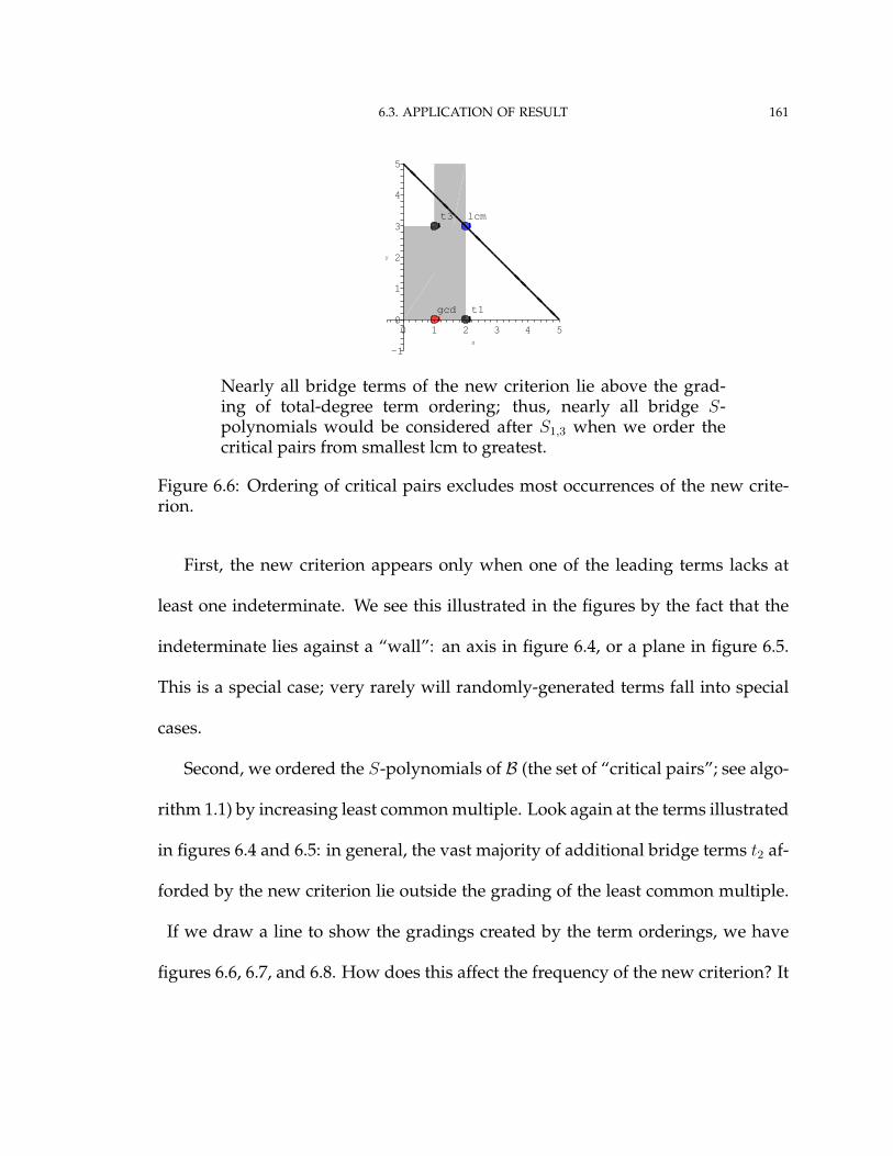
6.3. APPLICATION OF RESULT 161
0
t1
5
gcd
-1
y
5
x
4
2
0
1
3
t3
2
lcm3
1 4
Nearly all bridge terms of the new criterion lie above the grad-ing of total-degree term ordering; thus, nearly all bridge S-polynomials would be considered after S1,3 when we order thecritical pairs from smallest lcm to greatest.
Figure 6.6: Ordering of critical pairs excludes most occurrences of the new crite-rion.
First, the new criterion appears only when one of the leading terms lacks at
least one indeterminate. We see this illustrated in the figures by the fact that the
indeterminate lies against a “wall”: an axis in figure 6.4, or a plane in figure 6.5.
This is a special case; very rarely will randomly-generated terms fall into special
cases.
Second, we ordered the S-polynomials of B (the set of “critical pairs”; see algo-
rithm 1.1) by increasing least common multiple. Look again at the terms illustrated
in figures 6.4 and 6.5: in general, the vast majority of additional bridge terms t2 af-
forded by the new criterion lie outside the grading of the least common multiple.
If we draw a line to show the gradings created by the term orderings, we have
figures 6.6, 6.7, and 6.8. How does this affect the frequency of the new criterion? It

6.3. APPLICATION OF RESULT 162
0
t1
5
gcd
-1
y
5
x
4
2
0
1
3
t3
2
lcm3
1 4
All bridge terms of the new criterion lie above the grading of thislexicographic term ordering (x � y); thus, bridge S-polynomialswould be considered after S1,3 when we order the critical pairsfrom smallest lcm to largest. In this case, the selection of bridgeterms is reduced to Buchberger’s second criterion.
Figure 6.7: Ordering of critical pairs excludes most occurrences of the new crite-rion.
0
t1
4
-1
5
2
1
gcd
x
y
4
03
t3
2
lcm
51
3
"Most" bridge terms of the new criterion lie within the grad-ing of this lexicographic term ordering (y � x); thus, bridge S-polynomials would be considered before S1,3 when we order thecritical pairs from smallest lcm to largest.
Figure 6.8: Ordering of critical pairs excludes most occurrences of the new crite-rion.
6.3. APPLICATION OF RESULT 163
means that often we have a triplet that may satisfy the new criterion, but the algo-
rithm will almost always evaluate S1,3 before S1,2 and S2,3, the reverse of the order
needed for the new criterion to apply!
To test this latter hypothesis, we ran an experiment to estimate the area of re-
gions where one can find possible bridge terms. Increasing from two to six vari-
ables, we generated for each turn 1,000 random pairs of terms t1, t2. For each pair
of terms, we first calculated the area of the region from which Buchberger’s criteria
would give us a bridge term; since this region is a hypercube, it is immediate to de-
duce the area from the exponents. Then we calculated the area of the region from
which the new criterion would give us a bridge term. To avoid having to aver-
age the occasional “infinite” region, we restricted this region so that the maximum
degree of a bridge term could be no larger than that of the two endpoints. This
is a reasonable restriction, since the random terms we generated for tables were
also restricted in their maximum degree. Then we removed from the region any
bridge terms t3 that were larger than lcm (t1, t2) with respect to the term ordering.
To calculate the area, then, we simply counted the number of terms remaining in
the set.
Tables 6.4 and 6.5 show the results. As we see, the area of the regions also sug-
gest that the new criterion provides few additional possibilities for bridge terms.
We would caution the reader agaisnt comparing the data too closely to those of
tables 6.1 and 6.2; although we kept some conditions similar, we are comparing
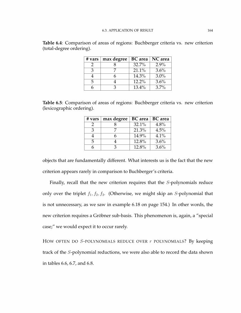
6.3. APPLICATION OF RESULT 164
Table 6.4: Comparison of areas of regions: Buchberger criteria vs. new criterion(total-degree ordering).
# vars max degree BC area NC area2 8 32.7% 2.9%3 7 21.1% 3.6%4 6 14.3% 3.0%5 4 12.2% 3.6%6 3 13.4% 3.7%
Table 6.5: Comparison of areas of regions: Buchberger criteria vs. new criterion(lexicographic ordering).
# vars max degree BC area BC area2 8 32.1% 4.8%3 7 21.3% 4.5%4 6 14.9% 4.1%5 4 12.8% 3.6%6 3 12.8% 3.6%
objects that are fundamentally different. What interests us is the fact that the new
criterion appears rarely in comparison to Buchberger’s criteria.
Finally, recall that the new criterion requires that the S-polynomials reduce
only over the triplet f1, f2, f3. (Otherwise, we might skip an S-polynomial that
is not unnecessary, as we saw in example 6.18 on page 154.) In other words, the
new criterion requires a Gröbner sub-basis. This phenomenon is, again, a ”special
case;” we would expect it to occur rarely.
HOW OFTEN DO S-POLYNOMIALS REDUCE OVER r POLYNOMIALS? By keeping
track of the S-polynomial reductions, we were also able to record the data shown
in tables 6.6, 6.7, and 6.8.
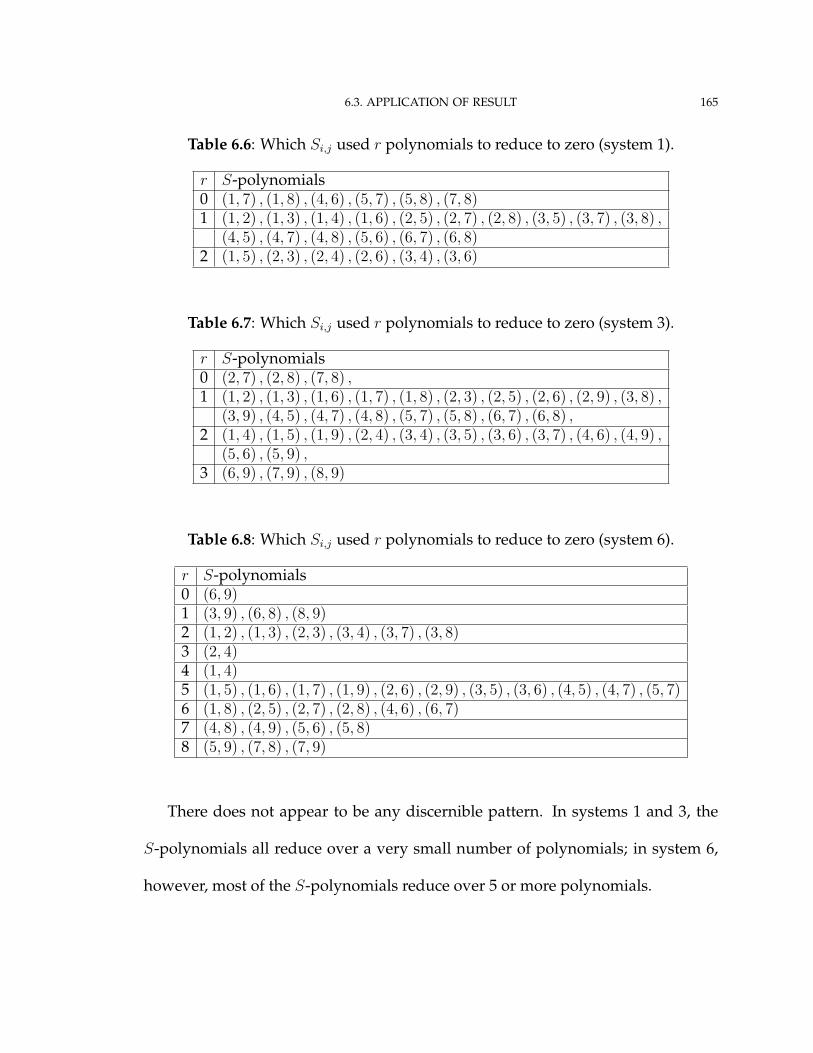
6.3. APPLICATION OF RESULT 165
Table 6.6: Which Si,j used r polynomials to reduce to zero (system 1).
r S-polynomials0 (1, 7) , (1, 8) , (4, 6) , (5, 7) , (5, 8) , (7, 8)1 (1, 2) , (1, 3) , (1, 4) , (1, 6) , (2, 5) , (2, 7) , (2, 8) , (3, 5) , (3, 7) , (3, 8) ,
(4, 5) , (4, 7) , (4, 8) , (5, 6) , (6, 7) , (6, 8)2 (1, 5) , (2, 3) , (2, 4) , (2, 6) , (3, 4) , (3, 6)
Table 6.7: Which Si,j used r polynomials to reduce to zero (system 3).
r S-polynomials0 (2, 7) , (2, 8) , (7, 8) ,1 (1, 2) , (1, 3) , (1, 6) , (1, 7) , (1, 8) , (2, 3) , (2, 5) , (2, 6) , (2, 9) , (3, 8) ,
(3, 9) , (4, 5) , (4, 7) , (4, 8) , (5, 7) , (5, 8) , (6, 7) , (6, 8) ,2 (1, 4) , (1, 5) , (1, 9) , (2, 4) , (3, 4) , (3, 5) , (3, 6) , (3, 7) , (4, 6) , (4, 9) ,
(5, 6) , (5, 9) ,3 (6, 9) , (7, 9) , (8, 9)
Table 6.8: Which Si,j used r polynomials to reduce to zero (system 6).
r S-polynomials0 (6, 9)1 (3, 9) , (6, 8) , (8, 9)2 (1, 2) , (1, 3) , (2, 3) , (3, 4) , (3, 7) , (3, 8)3 (2, 4)4 (1, 4)5 (1, 5) , (1, 6) , (1, 7) , (1, 9) , (2, 6) , (2, 9) , (3, 5) , (3, 6) , (4, 5) , (4, 7) , (5, 7)6 (1, 8) , (2, 5) , (2, 7) , (2, 8) , (4, 6) , (6, 7)7 (4, 8) , (4, 9) , (5, 6) , (5, 8)8 (5, 9) , (7, 8) , (7, 9)
There does not appear to be any discernible pattern. In systems 1 and 3, the
S-polynomials all reduce over a very small number of polynomials; in system 6,
however, most of the S-polynomials reduce over 5 or more polynomials.

6.3. APPLICATION OF RESULT 166
6.3.4. FINAL REMARK. The following “cute” fact provides an “alternate defini-
tion” of Buchberger’s criteria:
LEMMA 6.19. (A) and (B) where
(A) ∀x VB1xk(t1, t3) if and only if BC1 (t1, t3)
(B) ∀x VB2xk(t1, t2, t3) if and only if BC2 (t1, t2, t3)
PROOF. Immediate from the definitions of the criteria. �
Part 3
A New Criterion for Gröbner Basis Detection
of Two Polynomials

Chapter 7
Gröbner basis detection: introduction
7.1. INTRODUCTION TO THE PROBLEM
In previous chapters, we were given a term ordering� and the leading terms of
a set of polynomials with respect to �. We looked for criteria on the leading terms
that would guarantee that the polynomials were a Gröbner basis with respect to
�, so long as a certain number of S-polynomials reduced to zero.
Suppose instead that we only have a set of polynomials. Rather than picking
a term ordering and deciding whether the polynomials were a Gröbner basis with
respect to that term ordering, what if we searched for a term ordering that would
guarantee the polynomials were already a Gröbner basis? We are asking for criteria
that decide for given f1, . . . , fm
∃ � GB� (f1, . . . , fm)
168

7.1. INTRODUCTION TO THE PROBLEM 169
We illustrate the idea with example 7.1.
EXAMPLE 7.1. Let f1 = x + y, f2 = y + 1. We know from corollary 2.9 on page 69
that if their leading terms are
f1 = x f2 = y
then we can skip the reduction of their S-polynomial. Hence f1, f2 are a Gröbner
basis with respect to �= lex (x, y).
However, if �= lex (y, x), we have
f1 = y f2 = y
Then
S1,2 =lcm (y, y)
y· (x + y)− lcm (y, y)
y· (y + 1)
= (x + y)− (y + 1)
= x− 1
Observe that neither f1 nor f2 divides any term of S1,2. Hence
S1,2∗9
(f1,f2)0
and f1, f2 are not a Gröbner basis with respect to �= lex (x, y). �
7.1. INTRODUCTION TO THE PROBLEM 170
We do not expect to encounter many sets of polynomials where there exists
some term ordering such that the leading terms are all relatively prime. We shall
see that we may be able to detect a Gröbner basis nevertheless.
Why would we want to do this? For many Gröbner basis applications, any term
ordering will suffice: we don’t care if we have a total-degree term ordering, a lexi-
cographic term ordering, or some other term ordering altogether – all that matters
is the existence of a Gröbner basis with respect to some term ordering. One example
application would be the problem we used to introduce Gröbner bases: deciding
the existence and cardinality of common roots.
On the other hand, if a specific term ordering is needed – as in the case of
finding the common roots, where one typically uses a lexicographic ordering to
compute a Gröbner basis – it may still be useful to try detecting a Gröbner ba-
sis beforehand. Why? To pursue the example: a lexicographic term ordering is
generally agreed to give some of the least efficient performance from any algo-
rithm used to compute Gröbner bases, while a total-degree term ordering is more
efficient.1 In most of the cutting-edge work done with Gröbner bases, one com-
putes the Gröbner basis with respect to a “probably efficient” term ordering, then
employs a second algorithm that converts to the desired term ordering. Such algo-
rithms exist and are in use; see for example [FGLM93] and [CKM97]. Thus, if we
can detect that a system of polynomials is already a Gröbner basis with respect to
1See the remark on page 109 of [CLO97], who reference [BS87]; see also [CKM97] and [Tra05].

7.2. MATRIX REPRESENTATIONS OF TERM ORDERINGS 171
some term ordering, we could use that as a starting point to convert to the desired
term ordering.
A general solution for Gröbner basis detection already exists: Peter Gritzmann
and Bernd Sturmfels give it in [GS93]; we discuss this solution in chapter 8.
If there is already a general solution, why pursue more research in this area? The
general solution is not easily implemented. To our knowledge, there is no current
implementation. Indeed, Bernd Sturmfels and Markus Wiegelman followed the
first paper with a second that considered the special case of finding a term ordering
where all the leading terms are relatively prime; see [SW97].
We stumbled on our solution by accident. While conducting the research that
led to the results in chapter 6, we observed that Gröbner bases of two polynomials
had a special form. This led to a theorem; in turn, this theorem suggested an
algorithm for Gröbner basis detection that is easy to implement. How easy? The
author implemented the algorithm in two days (see [HP04]), most of which he
spent persuading Maple that it really could find solutions to strict inequalities. We
demonstrated this implementation at the 2004 Applications of Computer Algebra
conference at Lamar University in Beaumont, Texas.
7.2. MATRIX REPRESENTATIONS OF TERM ORDERINGS
Since “Gröbner basis detection” considers the question of whether a special
term ordering exists, we need a way to solve for term orderings. For this, we

7.2. MATRIX REPRESENTATIONS OF TERM ORDERINGS 172
need a convenient algebraic representation of term orderings. A well-established
technique allows us to represent any admissible term ordering as one of the most
familiar of mathematical objects: a matrix.
To treat the theory in full detail is beyond the scope of this thesis; the interested
reader should refer to [Rob86], [Wei87], and [HW99]. We give the results necessary
to understand our results and those of [GS93].
We adopt the following notational conventions:
• α, β represent column vectors;
• M, N represent matrices;
• α(i) represents row i of vector α, andM(i) represents row i of vec-
torM.
7.2.1. ADMISSIBLE MATRICES.
DEFINITION 7.2. For vectors α, β ∈ Rn we say α� β if
• α(1) > β(1), or
• α(1) = β(1) and α(2) > β(2), or
• . . .
• α(1) = β(1) and . . . and α(n−1) = β(n−1) and α(n) > β(n).
We say that α, β are exponent vectors if α, β ∈ Qn. A matrix M ∈ Rm×n is ad-
missible if it has full rank over Q (that is, its column rank over Q equals n) and if
M · α� 0 for all nonzero vectors α ∈ Zn≥0.

7.2. MATRIX REPRESENTATIONS OF TERM ORDERINGS 173
EXAMPLE 7.3. Let
M =
1 1 1
0 1 1
0 0 1
N =
1 −1 −1
0 2 2
0 0 1
We claim thatM is admissible, while N is not.
Proof thatM is admissible: Since detM 6= 0, it has full rank. Let α be a nonzero
vector in Z3≥0; then
M · α =
1 1 1
0 1 1
0 0 1
·
α(1)
α(2)
α(3)
=
α(1) + α(2) + α(3)
α(2) + α(3)
α(3)
Since α ∈ Z3
≥0 and α is nonzero, α(1), α(2), α(3) ≥ 0 and α(1) + α(2) + α(3) > 0. Hence
M · α� 0, as desired.
Proof thatN is not admissible: Let α =
(0 1 0
)T
. Clearly α ∈ Z3≥0. However,
N · α =
1 −1 −1
0 2 2
0 0 1
·
0
1
0

7.2. MATRIX REPRESENTATIONS OF TERM ORDERINGS 174
=
−1
2
0
� 0
�
Admissible matrices will prove useful because we can represent terms as expo-
nent vectors with integer entries. For an admissible matrixM, the product ofM(i)
with an exponent vector α represents a weight w for α. The product ofM with α
is a vector of weights w1, . . . , wm ∈ R. Theorem 7.5 will use these weight vectors to
show howM corresponds to a term ordering on the terms in x1, . . . , xn.
DEFINITION 7.4. Let M be an admissible matrix, and � be an admissible term
ordering. We say thatM is an admissible matrix representation of � if for every
pair of terms t, u, whose exponent vectors we denote as α, β,
t � u ⇔ M · α�M · β
In general, we will say thatM is a representation of �, or thatM induces �, or
that � inducesM.
It turns out that every admissible matrix induces a term ordering, and vice-
versa. This result is due to [Rob86, Wei87, HW99].

7.2. MATRIX REPRESENTATIONS OF TERM ORDERINGS 175
THEOREM 7.5. (A) and (B) where
(A) Every term ordering on terms in x1, . . . , xn is induced by an admissible matrix
M∈ Rm×n.
(B) Every admissible matrix M ∈ Rm×n induces a term ordering on T (x1, . . . , xn)
(the set of terms in x1, . . . , xn).
Before proving the theorem, we require some background material.
7.2.2. EXTENDING � FROM T (x1, . . . , xn) TO Qn. One thing we will need to do, is
extend a term ordering from an ordering on terms to an ordering on Qn. How do
we do this?2
Let � be an admissible term ordering. We can extend � to an ordering �Zn≥0
on
Zn≥0 directly: for α, β ∈ Zn
≥0
α �Zn≥0
β ⇔ xα(1)
1 · · ·xα(n)n � x
β(1)
1 · · ·xβ(n)n
Recall that, for terms, t, u, v, we know that
t � u ⇔ tv � uv
It follows that for all α, β, γ ∈ Zn≥0
(7.1) α �Zn≥0
β ⇔ α + γ �Zn≥0
β + γ
2The following argument appears in numerous sources before this one; for example, proposition1.4.14 and exercise 8 in chapter 1, section 4 of [KR00].

7.2. MATRIX REPRESENTATIONS OF TERM ORDERINGS 176
Now that we have �Zn≥0
, we can extend it immediately to an ordering on all of
Zn. For γ ∈ Zn, find α, β ∈ Zn≥0 such that γ = α− β. Begin by defining
γ �Zn 0 ⇔ α �Zn≥0
β
We have to check that the ordering is well defined here. Suppose γ = α−β = ζ−ϑ
for γ ∈ Zn, α, β, ζ, ϑ ∈ Zn≥0. Assume that α �Zn
≥0β; by (7.1), α + ϑ �Zn
≥0β + ϑ. Since
α = β + ζ − ϑ,
α + ϑ �Zn≥0
β + ϑ
(β + ζ − ϑ) + ϑ �Zn≥0
β + ϑ
β + ζ �Zn≥0
β + ϑ
Again by (7.1), we have ζ �Zn≥0
ϑ. Hence γ �Zn≥0
0 is well-defined. We complete
the definition by
γ �Zn≥0
ζ ⇔ γ − ζ �Zn≥0
0
How shall we extend the ordering to �Qn? We teach grade-school students to
compare rational numbers by finding a common denominator; the same technique
extends naturally to Qn. Proceed in the following way: for α, β ∈ Qn in sim-
plest form, let γ be the least common multiple of the denominators of α(1), . . . , α(n),
β(1), . . . , β(n). Notice that γ is a natural number, and hence a scalar with respect to
α, β. Then
α �Qn β ⇔ γ · α �Zn≥0
γ · β

7.2. MATRIX REPRESENTATIONS OF TERM ORDERINGS 177
The following example illustrates each of these techniques.
EXAMPLE 7.6. Let � represent the lexicographic ordering on x1, x2 with x1 � x2.
Consider α =
(1 3
)T
, β =
(0 2
)T
. Note that α, β ∈ Z2≥0. We have
x1x32 � x2
2 ⇒ α �Zn≥0
β
Thus
α− β �Zn 0
Continuing the extension,
α− β �Zn 0 ⇒ 0 �Zn β − α
(Put 0 = γ, ζ = β − α and use the definition for γ �Zn ζ .)
Let γ =
(−1 −1
)T
. Note that γ ∈ Z2 and γ = β − α. Hence 0 �Zn γ.
Finally, let ζ =
(1 −2
3
)T
and ϑ =
(34−2
)T
. The least common multiple
of the denominators is 12; since(
12 −8
)T
�Zn
(9 −24
)T
, we have ζ �Qn ϑ.
�
7.2.3. WEIGHT VECTORS FOR A SUBSPACE OF Qn. If we could assemble different
“weight vectors” that order different subspaces of Qn in accordance with �Qn , we
could construct a matrix that satisfies the requirements of theorem 7.5. How would
these weight vectors behave? Suppose ω was one such weight vector; we would
7.2. MATRIX REPRESENTATIONS OF TERM ORDERINGS 178
need
ω · α > ω · β ⇒ α �Qn β
Moreover, for the matrix to be admissible, we would also need the weight vectors
to be linearly independent over Q, and
ω · α > 0 ∀α ∈ Nn≥0
The following lemma, adapted with minor cosmetic changes from [HW99], pro-
vides a constructive proof that such weight vectors exist for any term ordering �.
It is an explicit construction that corresponds to a similar lemma in [Wei87].
LEMMA 7.7. Let �Qn be the extension to Qn of an admissible term ordering �. For any
non-trivial, Q-linear subspace U of Qn, ∃m ∈ Rn such that:
• m is in the R-linear extension of U
• m · x > 0 implies x �Qn 0
• x ∈ Zn≥0 implies m · x ≥ 0
PROOF. Let U be a non-trivial Q-linear subspace of Qn. We prove the lemma by
construction of m.
Let {v1, . . . , vs} be an arbitrary orthogonal Q-basis of U with v1, . . . , vs �Qn 0.
Let k be such that vk �Qn v1, . . . , vs.
For j = 1, . . . , s, let
γj = inf {q ∈ Q : qvk �Qn vj}
7.2. MATRIX REPRESENTATIONS OF TERM ORDERINGS 179
Let
m =s∑
i=1
γi ·vT
i
vTi · vi
We claim that m satisfies the requirements of the lemma.
Let x ∈ U be arbitrary, but fixed. Let x′1, . . . , x′s be the co-ordinates of x with
respect to v1, . . . , vs. Then
m · x =
(s∑
i=1
γi ·vT
i
vTi · vi
)·
(s∑
j=1
x′jvj
)
=s∑
i=1
s∑j=1
γix′j ·
vTi · vj
vTi · vi
For i 6= j, vi and vj are orthogonal, so vTi · vj = 0. Thus
m · x =s∑
i=1
γix′i
= γ · x′
Assume m · x > 0; then γ · x′ > 0. We want to show that x �Qn 0. Using the
continuity of the real line, choose γ′ ∈ Qn such that γ′ · x′ > 0 and
γ′j > γj if x′j < 0
γ′j < γj if x′j > 0
γ′j = 0 if x′j = 0
We claim that
0 ≺Qn (γ′ · x′) vk ≺Qn x
7.2. MATRIX REPRESENTATIONS OF TERM ORDERINGS 180
We have
0 ≺Qn (γ′ · x′) vk =
(s∑
j=1
γ′jx′j
)vk =
s∑j=1
γ′j(x′jvk
)Let j ∈ {1, . . . , s} be arbitrary, but fixed.
Case 1: x′j < 0
Then γ′j > γj . Recall that γj = inf {q ∈ Q : qvk �Qn vj}, so
γ′jvk �Qn vj
Multiplying both sides by the scalar x′j , we have
x′j ·(γ′jvk
)≺Qn x′k · vj
Case 2: x′j > 0
Then γ′j < γj . Recall again that γj = inf {q ∈ Q : qvk �Qn vj}. Then
γ′jvk ≺Qn γjvk �Qn vj
Multiplying both sides by the scalar x′j ,
x′j(γ′jvk
)≺Qn x′jvj
From cases 1 and 2,
0 ≺Qn (γ′ · x′) vk =
(s∑
j=1
γ′j · x′j
)vk =
s∑j=1
(x′j(γ′jvk
))≺
s∑j=1
x′jvj = x
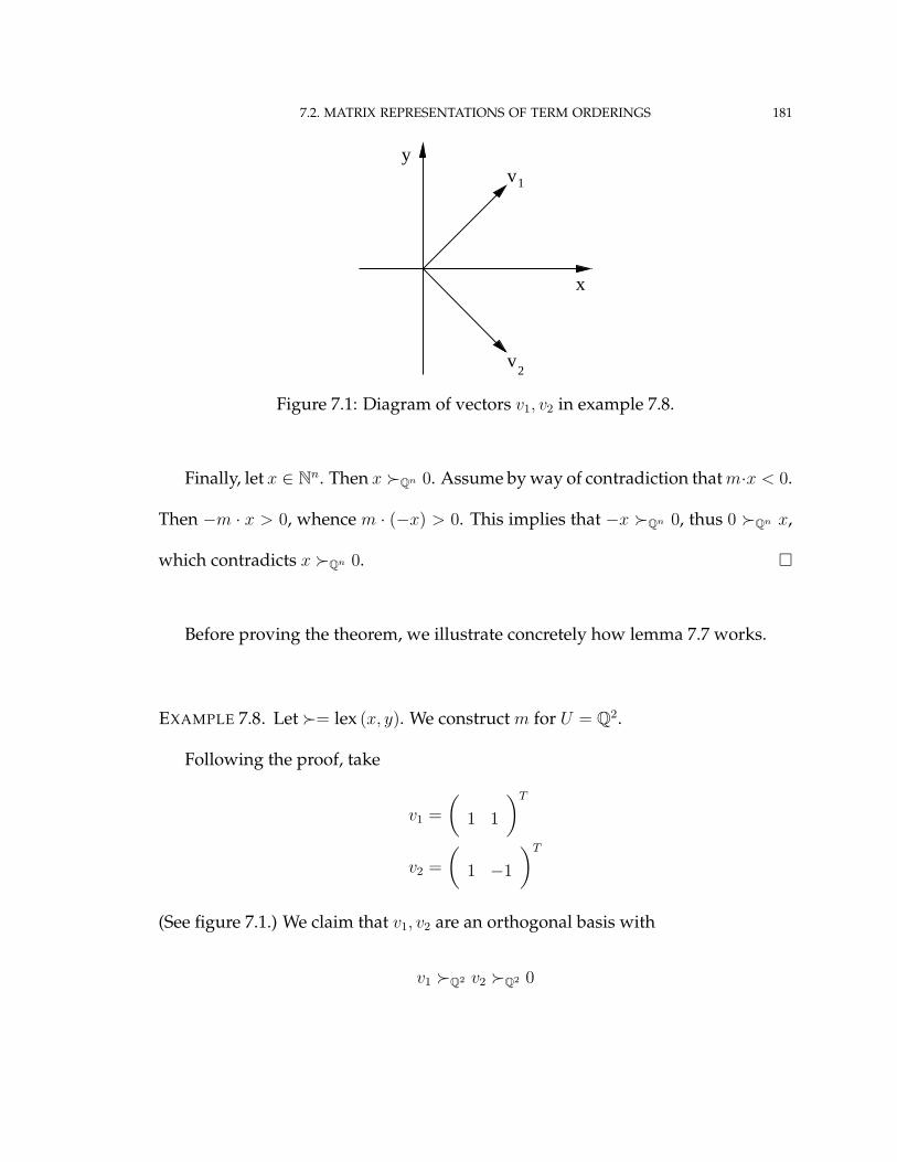
7.2. MATRIX REPRESENTATIONS OF TERM ORDERINGS 181
y1
v2
x
v
Figure 7.1: Diagram of vectors v1, v2 in example 7.8.
Finally, let x ∈ Nn. Then x �Qn 0. Assume by way of contradiction that m·x < 0.
Then −m · x > 0, whence m · (−x) > 0. This implies that −x �Qn 0, thus 0 �Qn x,
which contradicts x �Qn 0. �
Before proving the theorem, we illustrate concretely how lemma 7.7 works.
EXAMPLE 7.8. Let �= lex (x, y). We construct m for U = Q2.
Following the proof, take
v1 =
(1 1
)T
v2 =
(1 −1
)T
(See figure 7.1.) We claim that v1, v2 are an orthogonal basis with
v1 �Q2 v2 �Q2 0

7.2. MATRIX REPRESENTATIONS OF TERM ORDERINGS 182
For the orthogonality (which is geometrically clear),
v1 · v2 = 1− 1 = 0
We can see that the two vectors are linearly independent from∣∣∣∣∣∣∣∣1 1
1 −1
∣∣∣∣∣∣∣∣ = −2 6= 0
As for the ordering, it is intuitively clear from the geometry: compare how far right
the vectors lie, in case of a tie, how far up. Algebraically,
y2 � 1 ⇒(
0 2
)T
�Z2≥0
0 ⇒(
1 1
)T
−(
1 −1
)T
�Z2 0
and by extension (1 1
)T
�Q2
(1 −1
)T
A similar argument will show that(
1 −1
)T
�Q2 0.
Following the proof, we set
γ1 = inf {q ∈ Q : qv1 �Q2 v1}
Geometrically, this says that γ1 is the maximum scaling of v1 that is no larger than
itself with respect to �Q2 ; this is obviously 1. Similarly, set
γ1 = inf {q ∈ Q : qv1 �Q2 v2}

7.2. MATRIX REPRESENTATIONS OF TERM ORDERINGS 183
y
2
kv1
x
v
(a) kv1 for k < 1
y
2
kv1
x
v
(b) kv1 for k > 1
Figure 7.2: How lemma 7.7 generates γ1, γ2 for example 7.8.
Geometrically, this says that γ2 is the maximum scaling of v1 that is no larger than
v2 with respect to �Q2 : that is, the scaling of v1 whose rightmost entry is less than
or equal to the rightmost entry of v2. Again, this is 1; see figure 7.2.
Then
m = γ1 ·vT
1
vT1 v1
+ γ2 ·vT
2
vT2 v2
=
(1 1
)(
1 1
)·(
1 1
)T+
(1 −1
)(
1 −1
)·(
1 −1
)T
=
(1 1
)2
+
(1 −1
)2
=
(1 0
)
7.2. MATRIX REPRESENTATIONS OF TERM ORDERINGS 184
Not surprisingly, if we take
m · α
for any exponent vector α, m selects the first co-ordinate as the weight. This is
precisely the first test of the lexicographic ordering. �
7.2.4. PROOF OF THEOREM 7.5. Now we can prove theorem 7.5. We restate it and
present the proof:
THEOREM. (A) and (B) where
(A) Every term ordering on terms in x1, . . . , xn is induced by an admissible matrix
M∈ Rm×n.
(B) Every admissible matrix M ∈ Rm×n induces a term ordering on T (x1, . . . , xn)
(the set of terms in x1, . . . , xn).
PROOF. We prove (A) by construction.
Using lemma 7.7, findM(1) on Qn.
For i > 1, let Vj ={x ∈ Qn :M(j) · x = 0
}for j = 1, . . . , i − 1, and Ui = V1 ∩
· · · ∩ Vi−1. Using lemma 7.7, findM(i) for the non-trivial subspaces Ui of Qn.
Since dim Ui−1 > dim Ui and dim U1 < n, this process must terminate at some
trivial subspace Um = {0}. It is clear from the construction in the proof of lemma
7.7 thatM has full rank; we further haveM · x � 0 for x ∈ Nn\ {0}. HenceM is
admissible; also from the lemma,M induces �.

7.2. MATRIX REPRESENTATIONS OF TERM ORDERINGS 185
To prove (B), letM be arbitrary, but fixed. Define in the following way a rela-
tion �M on T (x1, . . . , xn), the set of terms in x1, . . . , xn: for all t, u ∈ T (x1, . . . , xn),
whose exponent vectors we denote as α, β,
t �M u ⇔ M · α�M · β
We claim that �M is an admissible term ordering. We verify that �M satisfies the
three parts of the definition.
First claim: ∀t 6= u ∈ T (x1, . . . , xn), t �M u or u �M t.
Let t, u ∈ T (x1, . . . , xn). Let α, β be the exponent vectors of t, u, respectively.
We approach by the contrapositive: assume neither t �M u nor u �M t. Then
M · α =M · β.
CertainlyM · α =M · β iffM · (α− β) = 0. SinceM has full rank, α = β.
Hence t = u.
So, t 6= u implies t �M u or u �M t.
Second claim: ∀t ∈ T (x1, . . . , xn), t 6= 1 implies t �M 1.
Let t ∈ T (x1, . . . , xn), and write α for the exponent vector of t. Observe that 0
is the exponent vector of 1.
Assume t 6= 1. We have α ∈ Zn≥0, and α 6= 0. By definition of an admissible
matrix,M · α� 0. ThusM · α�M · 0.
Hence t �M 1.
Third claim: ∀t, u, v ∈ T (x1, . . . , xn), t �M u implies tv �M uv.
7.3. SOLVING FOR ADMISSIBLE MATRICES 186
Let t, u, v ∈ T (x1, . . . , xn), and write α, β, γ for their exponent vectors, respec-
tively.
Assume t �M u. Then
M · α�M · β
M · α +M · γ �M · β +M · γ
M · (α + γ)�M · (β + γ)
It follows that tv �M uv.
We have shown that �M satisfies the three criteria for an admissible term or-
dering. SinceM was an arbitrary admissible matrix, we conclude that every ad-
missible matrix induces a term ordering on T (x1, . . . , xn). �
7.3. SOLVING FOR ADMISSIBLE MATRICES
Suppose we want a term ordering that satisfies a finite number of constraints.
The following theorem shows that we can construct an admissible matrix that in-
duces such a term ordering.
THEOREM 7.9. Let t1, . . . , t2r be terms with exponent vectors α1, . . . , α2r. We have
(A)⇔(B) where
(A) There exists an admissible term ordering � such that
t1 � t2 · · · t2r−1 � t2r
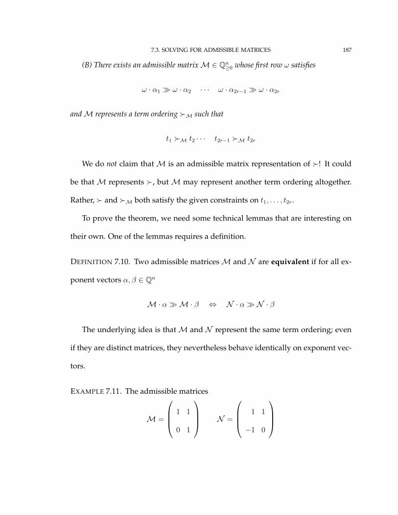
7.3. SOLVING FOR ADMISSIBLE MATRICES 187
(B) There exists an admissible matrixM∈ Qn≥0 whose first row ω satisfies
ω · α1 � ω · α2 · · · ω · α2r−1 � ω · α2r
andM represents a term ordering �M such that
t1 �M t2 · · · t2r−1 �M t2r
We do not claim thatM is an admissible matrix representation of �! It could
be that M represents �, but M may represent another term ordering altogether.
Rather, � and �M both satisfy the given constraints on t1, . . . , t2r.
To prove the theorem, we need some technical lemmas that are interesting on
their own. One of the lemmas requires a definition.
DEFINITION 7.10. Two admissible matricesM and N are equivalent if for all ex-
ponent vectors α, β ∈ Qn
M · α�M · β ⇔ N · α� N · β
The underlying idea is thatM and N represent the same term ordering; even
if they are distinct matrices, they nevertheless behave identically on exponent vec-
tors.
EXAMPLE 7.11. The admissible matrices
M =
1 1
0 1
N =
1 1
−1 0
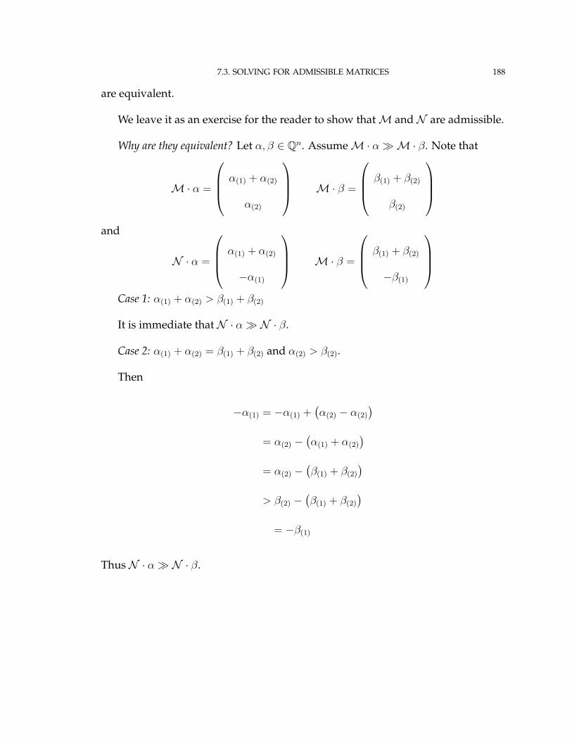
7.3. SOLVING FOR ADMISSIBLE MATRICES 188
are equivalent.
We leave it as an exercise for the reader to show thatM and N are admissible.
Why are they equivalent? Let α, β ∈ Qn. AssumeM · α�M · β. Note that
M · α =
α(1) + α(2)
α(2)
M · β =
β(1) + β(2)
β(2)
and
N · α =
α(1) + α(2)
−α(1)
M · β =
β(1) + β(2)
−β(1)
Case 1: α(1) + α(2) > β(1) + β(2)
It is immediate that N · α� N · β.
Case 2: α(1) + α(2) = β(1) + β(2) and α(2) > β(2).
Then
−α(1) = −α(1) +(α(2) − α(2)
)= α(2) −
(α(1) + α(2)
)= α(2) −
(β(1) + β(2)
)> β(2) −
(β(1) + β(2)
)= −β(1)
Thus N · α� N · β.

7.3. SOLVING FOR ADMISSIBLE MATRICES 189
We have shown that
M · α�M · β ⇒ N · α� N · β
A similar argument shows the converse.
Thus,M and N are equivalent. �
Now we present the lemmas. We use the notationM(i,j) to represent the entry
in row i, column j ofM.
The first lemma is proposition 1.4.12 on page 53 of [KR00].
LEMMA 7.12. For any admissible matrixM, the first non-zero entry in every column is
positive.
PROOF. We show the contrapositive. Suppose that entry j is the first nonzero
entry of column i ofM; suppose further thatM(i,j) < 0. Let α be the elementary
column vector ej ; that is, let α have one in the jth entry, and zeros elsewhere. Then
M · α =
0
...
0
M(i,j)
...
M(m,j)
Recall thatM(i,j) is negative. Then 0�M · α, soM is not admissible.
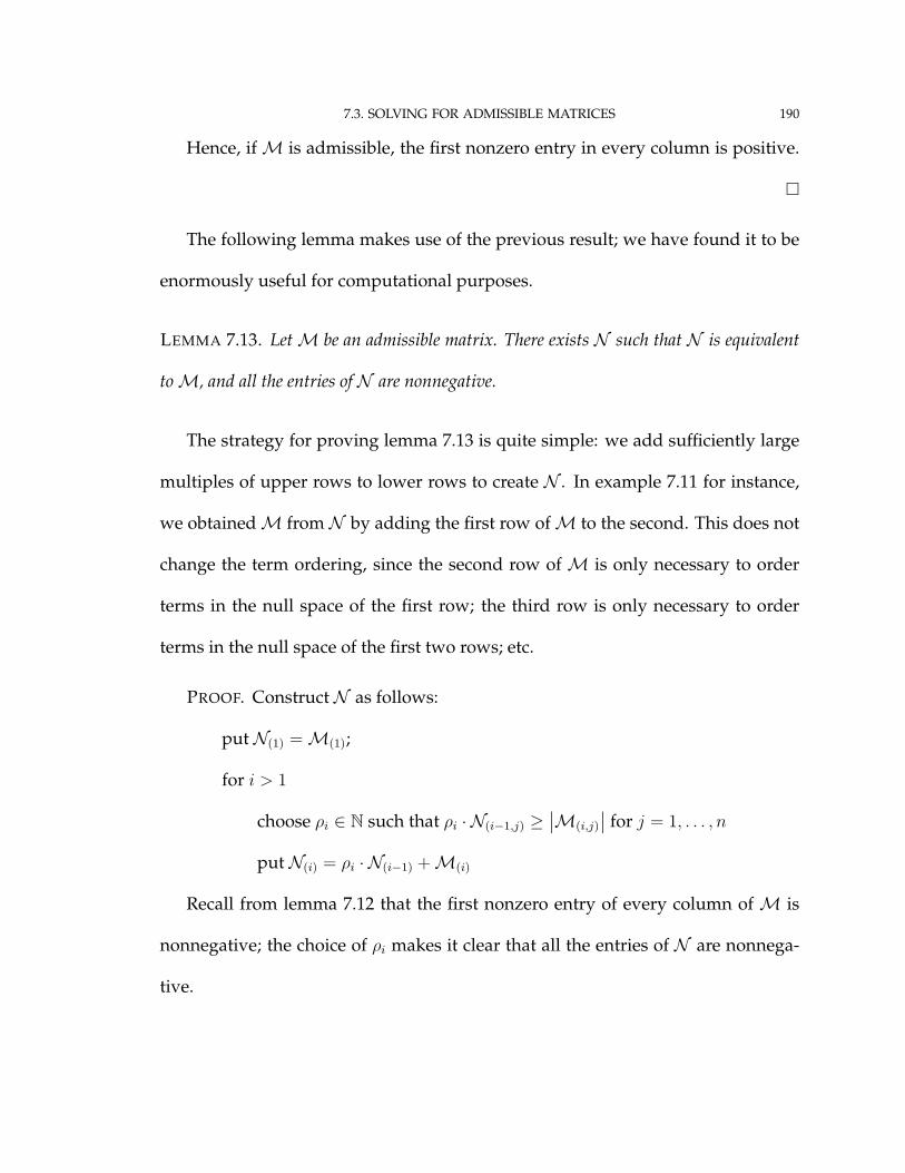
7.3. SOLVING FOR ADMISSIBLE MATRICES 190
Hence, ifM is admissible, the first nonzero entry in every column is positive.
�
The following lemma makes use of the previous result; we have found it to be
enormously useful for computational purposes.
LEMMA 7.13. LetM be an admissible matrix. There exists N such that N is equivalent
toM, and all the entries of N are nonnegative.
The strategy for proving lemma 7.13 is quite simple: we add sufficiently large
multiples of upper rows to lower rows to create N . In example 7.11 for instance,
we obtainedM from N by adding the first row ofM to the second. This does not
change the term ordering, since the second row of M is only necessary to order
terms in the null space of the first row; the third row is only necessary to order
terms in the null space of the first two rows; etc.
PROOF. Construct N as follows:
put N(1) =M(1);
for i > 1
choose ρi ∈ N such that ρi · N(i−1,j) ≥∣∣M(i,j)
∣∣ for j = 1, . . . , n
put N(i) = ρi · N(i−1) +M(i)
Recall from lemma 7.12 that the first nonzero entry of every column of M is
nonnegative; the choice of ρi makes it clear that all the entries of N are nonnega-
tive.

7.3. SOLVING FOR ADMISSIBLE MATRICES 191
Now we claim that, for all exponent vectors α, β ∈ Qn,M · α � M · β if and
only if N · α� N · β.
Let α, β ∈ Qn. AssumeM · α�M · β. Thus
M · (α− β)� 0
Hence, ∃R ∈ N such that
M(`) · (α− β)� 0 for ` = 1, . . . , R− 1
M(R) · (α− β) = 0
We claim that N(`) · (α− β) = 0 for ` = 1, . . . , R − 1 and N(R) · (α− β) > 0. We
proceed by induction on `.
Inductive base: SinceN(1) =M(1), it follows thatN(1)·(α− β) ≥ 0. The inequality
is strict only ifM(1) · (α− β) > 0; that is, if R = 1.
Inductive step: Let 1 < ` ≤ R, and assumeN(k) · (α− β) = 0 for 1 ≤ k < `. Recall
N(`) = ρ` · N(`−1) +M(`)
Then
N(`) · (α− β) =(ρ` · N(`−1) +M(`)
)· (α− β)
= ρ` · N(`−1) · (α− β) +M(`) · (α− β)
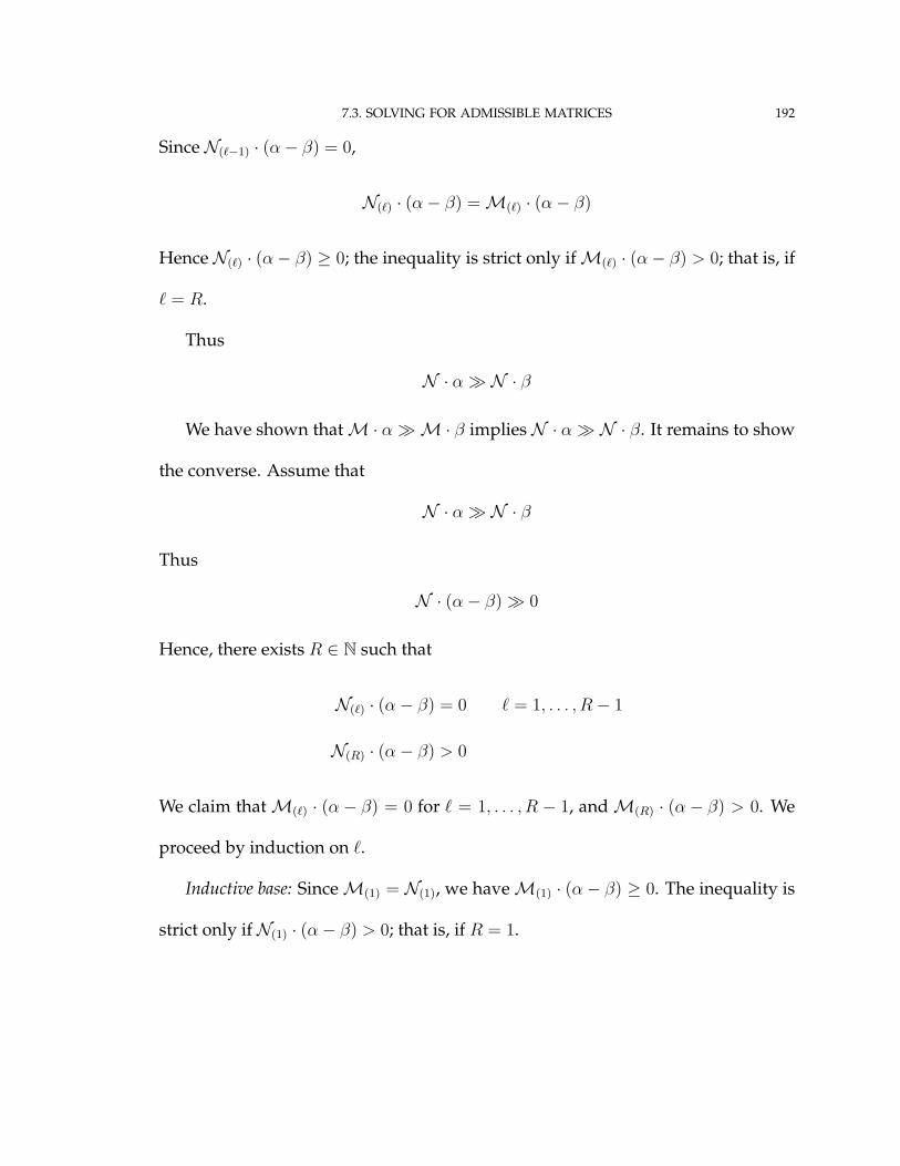
7.3. SOLVING FOR ADMISSIBLE MATRICES 192
Since N(`−1) · (α− β) = 0,
N(`) · (α− β) =M(`) · (α− β)
Hence N(`) · (α− β) ≥ 0; the inequality is strict only ifM(`) · (α− β) > 0; that is, if
` = R.
Thus
N · α� N · β
We have shown thatM · α�M · β implies N · α� N · β. It remains to show
the converse. Assume that
N · α� N · β
Thus
N · (α− β)� 0
Hence, there exists R ∈ N such that
N(`) · (α− β) = 0 ` = 1, . . . , R− 1
N(R) · (α− β) > 0
We claim thatM(`) · (α− β) = 0 for ` = 1, . . . , R − 1, andM(R) · (α− β) > 0. We
proceed by induction on `.
Inductive base: SinceM(1) = N(1), we haveM(1) · (α− β) ≥ 0. The inequality is
strict only if N(1) · (α− β) > 0; that is, if R = 1.

7.3. SOLVING FOR ADMISSIBLE MATRICES 193
Inductive step: For 1 < ` ≤ R, assume N(k) · (α− β) = 0 for 1 ≤ k < `. Recall
N(`) = ρ` · N(`−1) +M(`)
Then
N(`) · (α− β) =(ρ` · N(`−1) +M(`)
)· (α− β)
= ρ` · N(`−1) · (α− β) +M(`) · (α− β)
Since N(`−1) · (α− β) = 0, we have
M(`) · (α− β) = N(`) · (α− β) ≥ 0
The inequality is strict only if N(`) · (α− β) > 0; that is, if ` = R. Thus
M · α�M · β
We have shown that for arbitrary α, β ∈ Qn,
M · α�M · β ⇔ N · α� N · β
It follows that N has full column rank over Qn, and that N · α� 0 for all nonzero
α ∈ Qn. Hence N is admissible; it is equivalent toM; and all its entries are non-
negative. �
Now we prove theorem 7.9. At the end of the section, we discuss how the proof
suggests a way to construct a term ordering satisfying the requirements of clause
(A) of the theorem, assuming such a term ordering exists. First we restate the theorem:

7.3. SOLVING FOR ADMISSIBLE MATRICES 194
THEOREM. Let t1, . . . , t2r be terms with exponent vectors α1, . . . , α2r. We have (A)⇔(B)
where
(A) There exists an admissible term ordering � such that
t1 � t2 · · · t2r−1 � t2r
(B) There exists an admissible matrixM∈ Qn×n≥0 whose first row ω satisfies
ω · α1 � ω · α2 · · · ω · α2r−1 � ω · α2r
andM represents a term ordering �M such that
t1 �M t2 · · · t2r−1 �M t2r
PROOF. That (A)⇐(B) is immediate, sinceM induces a term ordering that sat-
isfies (A). It remains to show that (A)⇒(B).
Assume (A). We have an admissible term ordering � such that
τ1 � τ2 τ3 � τ4 · · · τ2r−1 � τ2r
Claim 1: We claim that ∃ω ∈ Rn≥0 satisfying
ω · α1 > ω · α2 · · · ω · α2r−1 > ω · α2r
LetM be an admissible matrix representation of �. Certainly
M · α1 �M · α2 · · · M · α2r−1 �M · α2r

7.3. SOLVING FOR ADMISSIBLE MATRICES 195
(If M · α2i−1 6� M · α2i, then τ2i−1 � τ2i, which contradicts the hypothesis.) By
lemma 7.13, we may assume that the entries ofM are nonnegative. Thus we can
put ω ∈ Rn≥0 such that
ω = ρ1M(1) + ρ2M(2) + · · ·+ ρmM(m)
where ρm = 1 and for k = 1, . . . ,m − 1 ρk ∈ N is sufficiently large that for every
` = 1, . . . , r
ρk
∣∣M(k) · (α2`−1 − α2`)∣∣ > ρk+1
∣∣M(k+1) · (α2`−1 − α2`)∣∣
+ · · ·
+ ρm
∣∣M(m) · (α2`−1 − α2`)∣∣
We claim that for ` = 1, . . . , r we have
ω · (α2`−1 − α2`) > 0
Let j ∈ {1, . . . , r}. UsingM · α2j−1 �M · α2j , choose R such that such that
M(`) · (α2j−1 − α2j) = 0 ∀` = 1, . . . , R− 1
M(R) · (α2j−1 − α2j) > 0
Then
ω · (α2j−1 − α2j) =(ρ1M(1) + · · ·+ ρmM(m)
)· (α2j−1 − α2j)
= ρ1M(1) · (α2j−1 − α2j) + · · ·+ ρmM(m) · (α2j−1 − α2j)
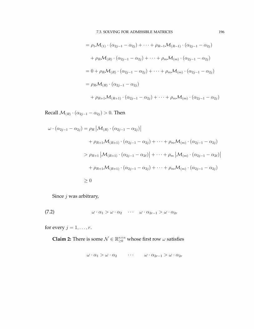
7.3. SOLVING FOR ADMISSIBLE MATRICES 196
= ρ1M(1) · (α2j−1 − α2j) + · · ·+ ρR−1M(R−1) · (α2j−1 − α2j)
+ ρRM(R) · (α2j−1 − α2j) + · · ·+ ρmM(m) · (α2j−1 − α2j)
= 0 + ρRM(R) · (α2j−1 − α2j) + · · ·+ ρmM(m) · (α2j−1 − α2j)
= ρRM(R) · (α2j−1 − α2j)
+ ρR+1M(R+1) · (α2j−1 − α2j) + · · ·+ ρmM(m) · (α2j−1 − α2j)
RecallM(R) · (α2j−1 − α2j) > 0. Then
ω · (α2j−1 − α2j) = ρR
∣∣M(R) · (α2j−1 − α2j)∣∣
+ ρR+1M(R+1) · (α2j−1 − α2j) + · · ·+ ρmM(m) · (α2j−1 − α2j)
> ρR+1
∣∣M(R+1) · (α2j−1 − α2`)∣∣+ · · ·+ ρm
∣∣M(m) · (α2j−1 − α2`)∣∣
+ ρR+1M(R+1) · (α2j−1 − α2j) + · · ·+ ρmM(m) · (α2j−1 − α2j)
≥ 0
Since j was arbitrary,
(7.2) ω · α1 > ω · α2 · · · ω · α2r−1 > ω · α2r
for every j = 1, . . . , r.
Claim 2: There is some N ∈ Rn×n≥0 whose first row ω satisfies
ω · α1 > ω · α2 · · · ω · α2r−1 > ω · α2r
7.3. SOLVING FOR ADMISSIBLE MATRICES 197
and N represents a term ordering �N such that
t1 �N t2 · · · t2r−1 �N t2r
Define N as follows:
• Let N(1) = ω, where ω is constructed to satisfy claim 1.
• Let
E = {e1, . . . , en} ⊂ N1×n where ei = (δik)nk=1
(By δik, we mean the Kronecker delta.)
• Fill the remaining n − 1 rows of N with E\ej where j is the first
nonzero element of u.
Observe that N has rank n, since the permutation(
1 j j − 1 · · · 3 2
)on
the rows of N gives an upper-triangular matrix. Furthermore, all the entries of N
are nonnegative, so N · α � 0 for all vectors α ∈ Zn≥0. Hence N is an admissible
matrix.
Let �N be the term ordering induced by N . Since ω is the first row of N and ω
was constructed as in claim 1, it follows from (7.2) that
τ1 �N τ2 · · · τ2r−1 �N τ2r
Thus N satisfies (B).
Claim 3: There is some N ′ ∈ Qn×n≥0 that satisfies (B).

7.3. SOLVING FOR ADMISSIBLE MATRICES 198
Let N be constructed as in claim 2, with first row ω. If ω ∈ Qn, then we are
done, for N ∈ Qn×n≥0 . Otherwise, let R be the number of irrational elements of
ω. We claim that we can construct v ∈ Rn≥0 with R − 1 irrational elements, and v
satisfies
v · α1 > v · α2 · · · v · α2r−1 > v · α2r
We prove this claim by applying the following algorithm:
Step 1: Let i be such that ω(i) is irrational.
Step 2: For unknown zi define
z =
(ω(1) · · · ω(i−1) zi ω(i+1) · · · ω(n)
)Step 3: Let
ε = infzi∈R
∃j z·α2j≤z·α2j+1
{∣∣zi − ω(i)
∣∣} ∈ R
Clearly ε > 0, since ω · α2j > ω · α2j+1 for every j = 1, . . . , r.
Step 4: Use the density of the rationals in the reals to choose vi ∈ Q≥0 such that
∣∣vi − ω(i)
∣∣ < ε
Step 5: Put
v =
(ω(1) · · · ω(i−1) vi ω(i+1) · · · ω(n)
)Since
∣∣vi − ω(i)
∣∣ < ε,
v · α1 > v · α2 · · · v · α2r−1 > v · α2r

7.3. SOLVING FOR ADMISSIBLE MATRICES 199
Step 6: If v ∈ Qn≥0, we are done; otherwise, repeat steps 1–6 with v in place of ω.
Each iteration finds a vector with R − 1 irrational elements, so this algorithm
terminates in at most n iterations with v ∈ Qn≥0 satisfying
(7.3) v · α1 > v · α2 · · · v · α2r−1 > v · α2r
Construct N ′ from N by replacing N(1) with v. Since we have replaced ω by v,
N ′ ∈ Qn×n≥0 . Since v satisfies (7.3), N ′ satisfies (B). �
We conclude with a brief discussion on how to construct a term ordering to
satisfy clause (A) of theorem 7.9.
First, we determine constraints on the exponent vectors of the terms in (A);
these constraints are as given for ω in (B). By the theorem, a term ordering satisfy-
ing (A) exists only if there exists a row vector ω ∈ Qn≥0 that satisfies (B). Further-
more, the proof of claim 2 shows how to construct a matrix M satisfying (B) by
adjoining elementary row vectors to ω: if j is the first non-zero entry of ω, adjoin
E\ej , where ej are the elementary row vectors described.
Thus, for given t1, . . . , t2r−1, the problem reduces to solving the inequalities
in (B) for ω(1), . . . , ω(n): that is, finding a rational solution to a system of integer
inequalities. The solution to this latter problem is well-established in the literature.

Chapter 8
Gröbner basis detection: general solution by
polytopes
8.1. PROBLEM
In 1993, Peter Gritzmann and Bernd Sturmfels [GS93] used Minkowski sums
of Newton polyhedra to find an algorithm for Gröbner basis detection. That is,
they found an algorithm that solves
∃ � GB� (f1, . . . , fm)
This chapter serves as a review of their result; we contribute nothing new to
their research. Readers familiar with Newton polyhedra and Minkowski sums
may choose to skip to section 8.3.
200

8.2. POLYTOPES, POLYHEDRA AND MINKOWSKI SUMS 201
8.2. POLYTOPES, POLYHEDRA AND MINKOWSKI SUMS
The reader may need to review the background material on term diagrams; see
section 2.5 on page 71.
A two-dimensional Newton polytope is similar to a term diagram, in that we
plot terms in the positive quadrant of an x-y axis. However, rather than represent
the leading terms of several polynomials, a Newton polytope encloses all the terms
of one polynomial in the smallest possible convex polygon.
The following definition is adapted from those found on pages 290 and 291 of
[CLO98] and page 247 of [GS93].
DEFINITION 8.1. For any finite set A = {m1, . . . ,mr} ⊂ Rn, its polytope is{λ1m1 + · · ·+ λrmr : λi ≥ 0,
r∑i=1
λi = 1
}
The Newton polytope N (f) of the polynomial f is the polytope enclosing the
points corresponding to the exponent vectors of the terms of f .
EXAMPLE 8.2. Let
f = x2y + 3xy − x + 7y3
The Newton polytope of f is given in figure 8.1.1 �
We can manipulate the Newton polytope to obtain a so-called Newton polyhe-
dron. The following definition comes from page 250 of [GS93]:
1Images of the convex polytopes in figures 8.1–8.4 were generated using [Fra04].

8.2. POLYTOPES, POLYHEDRA AND MINKOWSKI SUMS 202
4
4
3
3
2
1
20
10
Figure 8.1: Newton polytope of f in example 8.2.
2
3
1
0210 5
5
4
4
3
Figure 8.2: Newton polyhedron of f in example 8.2 (first quadrant view only).
DEFINITION 8.3. The Newton polyhedron of the polynomial f is the set
Naff (f) ={a + b : a ∈ N (f) , b ∈ Rn
≤0
}Visually, a polynomial’s polyhedron looks as if the corresponding polytope is
casting its shadow onto the axes; see figure 8.2.
Next we introduce the Minkowski sum of polytopes and polyhedra, taken from
pg. 246 of [GS93].
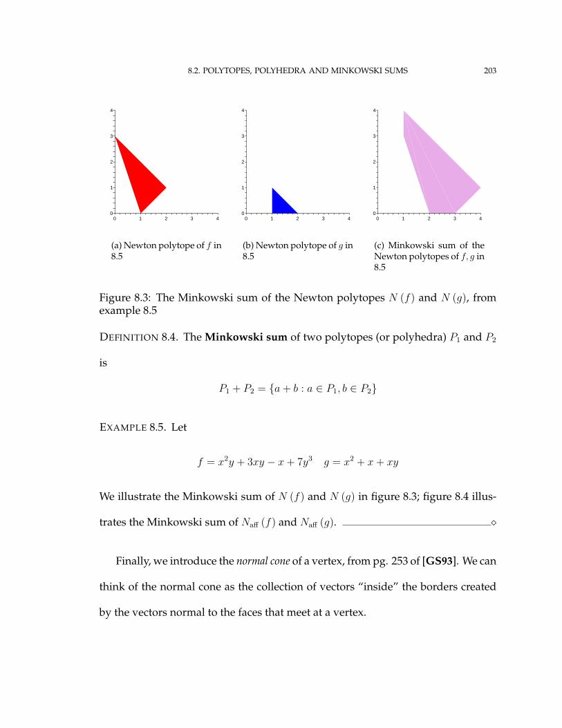
8.2. POLYTOPES, POLYHEDRA AND MINKOWSKI SUMS 203
4
4
3
3
2
1
20
10
(a) Newton polytope of f in8.5
4
4
3
3
2
1
20
10
(b) Newton polytope of g in8.5
4
4
3
3
2
1
20
10
(c) Minkowski sum of theNewton polytopes of f, g in8.5
Figure 8.3: The Minkowski sum of the Newton polytopes N (f) and N (g), fromexample 8.5
DEFINITION 8.4. The Minkowski sum of two polytopes (or polyhedra) P1 and P2
is
P1 + P2 = {a + b : a ∈ P1, b ∈ P2}
EXAMPLE 8.5. Let
f = x2y + 3xy − x + 7y3 g = x2 + x + xy
We illustrate the Minkowski sum of N (f) and N (g) in figure 8.3; figure 8.4 illus-
trates the Minkowski sum of Naff (f) and Naff (g). �
Finally, we introduce the normal cone of a vertex, from pg. 253 of [GS93]. We can
think of the normal cone as the collection of vectors “inside” the borders created
by the vectors normal to the faces that meet at a vertex.

8.2. POLYTOPES, POLYHEDRA AND MINKOWSKI SUMS 204
2
3
1
0210 5
5
4
4
3
(a) Newton polyhedron off in 8.5
2
3
1
0210 5
5
4
4
3
(b) Newton polyhedron ofg in 8.5
2
3
1
0210 5
5
4
4
3
(c) Minkowski sum ofNewton polyhedra of f, gin 8.5
Figure 8.4: The Minkowski sum of the Newton polyhedra Naff (f) and Naff (g), fromexample 8.5
DEFINITION 8.6. Let P be a Newton polytope (or polyhedron); let F be a face of P ,
and let v be a vertex of P . The normal cone of F is the relatively open collection of
outer normal vectors of P on the interior of F ; the normal cone of v is the collection
of vectors lying within the limiting faces of the normal cones of each face that meets
at v.
EXAMPLE 8.7. Let P be the Minkowski sum of the Newton polyhedra of
f = x2y + 3xy − x + 7y3 g = x2 + x + xy
(see figure 8.4). The normal cones of P are illustrated in figure 8.5; they lie within
the dotted lines. �
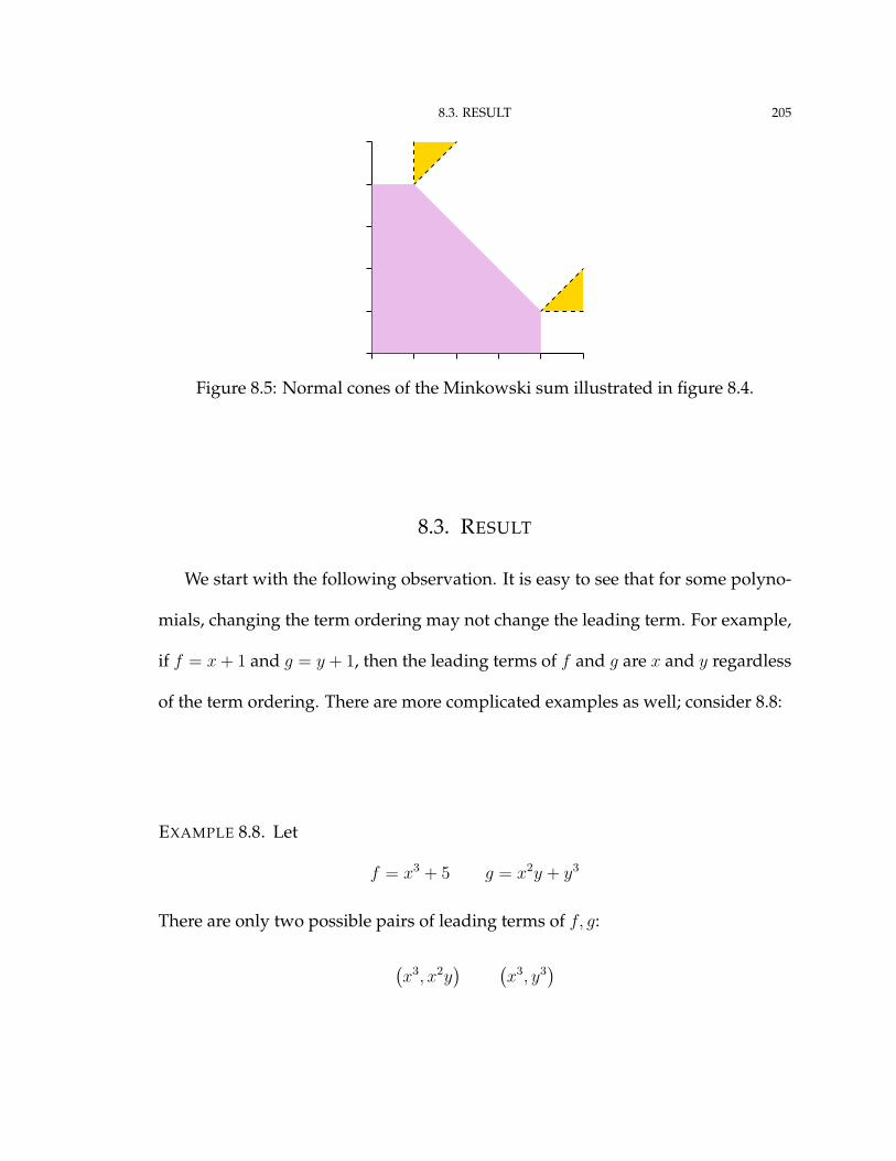
8.3. RESULT 205
Figure 8.5: Normal cones of the Minkowski sum illustrated in figure 8.4.
8.3. RESULT
We start with the following observation. It is easy to see that for some polyno-
mials, changing the term ordering may not change the leading term. For example,
if f = x + 1 and g = y + 1, then the leading terms of f and g are x and y regardless
of the term ordering. There are more complicated examples as well; consider 8.8:
EXAMPLE 8.8. Let
f = x3 + 5 g = x2y + y3
There are only two possible pairs of leading terms of f, g:
(x3, x2y
) (x3, y3
)
8.3. RESULT 206
Let �1= lex (x, y), �2= lex (y, x), and �3= tdeg (x, y). We have
lt�1 (f) = x3 lt�1 (g) = x2y
lt�2 (f) = x3 lt�2 (g) = y3
lt�3 (f) = x3 lt�3 (g) = x2y
We see that �1 and �3 have the same leading terms; we might say that they are
equivalent with respect to {f, g}. On the other hand, �2 has different leading
terms, so it is not equivalent to �1 and �3. �
We can generalize this observation with the following definition:
DEFINITION 8.9. Two term orderings �1 and �2 are said to be equivalent with
respect to F = {f1, . . . , fm} if
lt�1 (f1) = lt�2 (f1) · · · lt�1 (fm) = lt�2 (fm)
It is obvious that this relation satisfies the axioms of an equivalent relation: it is
reflexive, symmetric, and transitive.
A result of Teo Mora and Lorenzo Robbiano [MR88] is that given any set of
polynomials F = {f1, . . . , fm}, there are finitely many equivalence classes of term
orderings with respect to F . The consequence is that we can collect all terms or-
derings into a finite number of equivalence classes with respect to F .
Gritzmann and Sturmfels point out that, since there are finitely many equiva-
lence classes of term orderings, we can solve Gröbner basis detection by choosing

8.3. RESULT 207
a representative � from each class, then reducing the S-polynomials with respect
to �. If all of them reduce to zero for a given representative �, then we know that
f1, . . . , fm are a Gröbner basis with respect to �.
The question becomes, how do we find the equivalence classes, then a representa-
tive term orderings of each equivalence class? The answer is found in the following
theorem, which is proposition 3.2.1 of [GS93].
THEOREM 8.10. Let f1, . . . , fm ∈ F[x1, . . . , xn], and let M be the Minkowski sum of
Naff (f1) , . . . , Naff (fm). The vertices of M are in a one-to-one correspondence with the
equivalence classes of term orderings with respect to {f1, . . . , fm}.
Using this fact, one can fashion an algorithm for Gröbner basis detection; see
algorithm 8.1. The algorithm works in the following manner: from the normal
cone of each vertex of M , choose an integer vector ω. The product of ω and the
exponent vectors of f1, . . . , fm gives greatest weight to those terms whose exponent
vectors sum to the given vertex of M . We then extend ω to a term ordering� using
theorem 7.9 on page 186. We calculate the S-polynomials with respect to �. If all
the S-polynomials reduce to zero, we can report success with �; otherwise, we
proceed to the next normal cone. If none of the normal cones produces a term
ordering that gives us a Gröbner basis for f1, . . . , fm, we can report that no such
term ordering exists. We know that the algorithm terminates correctly, because
there are finitely many vertices, hence finitely many normal cones from which to

8.3. RESULT 208
Algorithm 8.1 GB_Detection_by_Minkowski_Sums
Inputs: f1, . . . , fm ∈ F[x1, . . . , xn]
Outputs: � such that GB� (f1, . . . , fm) if such � exists; NULLotherwise
M ← N (Naff (f1) + · · ·+ Naff (fm))
Compute v1, . . . , vr, the vertices of M
Loop k = 1, . . . , r
Pick ck from the normal cone of vk
Extend ck to an admissible matrixM
If GB�M (f1, . . . , fm) Then
Return �M
Return NULL
pick a representative, and because the weight vectors from these normal cones
characterize the equivalence classes of term orderings completely.

Chapter 9
Gröbner basis detection of two polynomials
by factoring
9.1. PROBLEM
We consider the following special case of the general Gröbner basis detection
problem: an algorithm for
∃ � GB� (f1, f2)
We present a new solution to this problem in section 9.3.1; it follows from theorem
9.1.
9.2. RESULT
THEOREM 9.1. For all f1, f2 ∈ F[x1, . . . , xn], for all term orderings �, the following are
equivalent:
(A) GB� (f1, f2)
209
9.2. RESULT 210
(B) gcd ( c1 , c2 ) = 1 where f1 = c1g, f2 = c2g ∃c1, c2, g ∈ F[x1, . . . , xn]
A brief example before we prove the theorem.
EXAMPLE 9.2. Let �1= lex (x, y), �2= lex (b, x, y),and
f1 = xy + bx f2 = x2 − bx
Note that
f1 = x (y + b) f2 = x (x− b)
The greatest common divisor of f1, f2 is g = x; its cofactors are
c1 = y + b c2 = x− b
Then
lt�1 (c1) = y lt�1 (c2) = x
while
lt�1 (c1) = b lt� (c2) = b
By theorem 9.1, f1, f2 are a Gröbner basis with respect to �1, because the leading
terms of c1 and c2 are relatively prime. Since the leading terms of c1, c2 are not
relatively prime with respect to �2, f1, f2 are not a Gröbner basis with respect to
�2. �
The proof of the theorem is short, because we unload the details into .
PROOF. (of theorem 9.1) Let f1, f2,� be arbitrary, but fixed.

9.2. RESULT 211
(B)⇒(A) is a consequence of lemma 1.37 on page 51; the requirement that
Sf1,f2 have a representation modulo f1, f2 is satisfied by the assumption of (B) that
gcd ( c1 , c2 ) = 1 and theorem 2.4 on page 59.
(A)⇒(B): Let f1, f2, � be arbitrary but fixed. Assume GB� (f1, f2). Then ∃h1, h2
such that h1, h2 give a representation of S� (f1, f2) modulo f1, f2. Recall σ12 and σ21
from definition 1.34 on page 48.
We have
S� (f1, f2) = h1f1 + h2f2
σ12f1 − σ21f2 = h1f1 + h2f2
(σ12 − h1) f1 = (σ21 + h2) f2(9.1)
From lemma 1.36 on page 50,
σ12 − h1 = σ12σ21 + h2 = σ21
Write
c1 = σ21 + h2 c2 = σ12 − h1
From (9.1),
(9.2) c2f1 = c1f2
Observe that c2 divides the left-hand side of (9.2), so it must divide the right-hand
side. By 1.35 on page 49, their leading monomials σ12 and σ21 are relatively prime

9.2. RESULT 212
on their indeterminates. So c1 and c2 have no common factors. Hence
c1 | f1 and c2 | f2
Let g1, g2 be such that
f1 = c1g1 and f2 = c2g2
Recall (9.2):
c2f1 = c1f2
c2 (c1g1) = c1 (c2g2)
g1 = g2
Let g = g1; it is clear that
f1 = c1g and f2 = c2g
and
gcd ( c1 , c2 ) = gcd ( σ21 , σ12 ) = 1
as claimed. �
The proof of (A)⇒(B) has the following interesting corollary:
COROLLARY 9.3. For all f1, f2 ∈ F [x1, . . . , xn] and for all term orderings �, if h1, h2
give a representation of Sf1,f2 modulo f1, f2, then
gcd (f1, f2) =f1
σ21 + h2
=f2
σ12 − h1

9.3. APPLICATION OF RESULT 213
PROOF. Let f1, f2,� be arbitrary, but fixed. We saw above that for some g,
f1 = (σ21 + h2) · g
f2 = (σ12 − h1) · g
We also observed that σ21 + h2 and σ12 − h1 were relatively prime. Thus g is the
greatest common divisor of f1, f2. Dividing each equation by the cofactor of g gives
corollary. �
9.3. APPLICATION OF RESULT
9.3.1. AN ALGORITHM FOR THEOREM 9.1. Theorem 9.1 tells us that two polyno-
mials are a Gröbner basis with respect to a term ordering if and only if the leading
terms of the cofactors of their greatest common divisor are relatively prime. For
any pair of relatively prime terms taken from each cofactor, theorem 9.1 provides
us with constraints like those of theorem 7.9 on page 186.
From theorem 7.9 we can find a matrix representationM∈ Qn of a term order-
ing that satisfies the constraints – assuming such a term ordering exists. We rewrite
the constraints as linear inequalities on the first row ofM (called u in the theorem)
and solve the inequalities. We fill the remaining rows of M with appropriately-
chosen elementary row vectors.
We have outlined this as algorithm 9.1.

9.3. APPLICATION OF RESULT 214
Algorithm 9.1 TO_for_GB
Inputs: f1, f2 ∈ F[x1, . . . , xn]
Output: � such that GB� (f1, f2) if such � exists; NULLotherwise
c1 ← cofactor of gcd (f1, f2) in f1
c2 ← cofactor of gcd (f1, f2) in f2
P = {(t1, t2) : tk is a term of ck}
— remove pairs that are not relatively prime
For p ∈ P
If gcd (t1, t2) 6= 1 Then
P ← P\p
— search for the desired term ordering �
For p ∈ P
�← Exists_tord_with_given_leadterms(t1, t2, f1, f2)
If � 6= NULLThen
Return �
— if we get this far, no term ordering exists
Return NULL
Algorithm 9.1 requires an additional algorithm, which we present as algorithm
9.2. Given t1, t2, f1, f2, this latter algorithm finds a term ordering such that f1 = t1
and f2 = t2, assuming such a term ordering exists. Note that the inequalities of
algorithm 9.2 solve for a weight vector ω; to extend this to a full term ordering, we
need to employ the technique indicated in the discussion at the end of section 7.3.

9.3. APPLICATION OF RESULT 215
Algorithm 9.2 Exists_Tord_with_given_leadterms
Inputs: terms t1, t2, polynomials f1, f2 ∈ F[x1, . . . , xn]
Output: � such that t1 = lt� (f1), t2 = lt� (f2) if such � exists; NULLotherwise
For i = 1, . . . , n
αi ← degxit1
βi ← degxit2
F1 ← {u : u is a trailing term of f1}
F2 ← {v : v is a trailing term of f2}
inequalities ← {}
For u ∈ F1
For i = 1, . . . , n
γi ← degxiu
inequalities ← inequalities
∪{ω1α1 + · · ·+ ωnαn > ω1γ1 + · · ·+ ωnγn}
For v ∈ F2
For i = 1, . . . , n
γi ← degxiv
inequalities ← inequalities
∪{ω1β1 + · · ·+ ωnβn > ω1γ1 + · · ·+ ωnγn}
If inequalities are feasible Then
Return solution of inequalities
Else
Return NULL

9.3. APPLICATION OF RESULT 216
Algorithms 9.1 and 9.2 are unoptimized beyond the requirements of theorem
9.1. There is one obvious optimization: terms that divide other terms cannot pos-
sibly be leading terms. Hence they can be left out of the construction of P in al-
gorithm 9.1 and of F1 and F2 in algorithm 9.2. Our Maple implementation [HP04]
includes these optimizations.
9.3.2. EXAMPLES OF THEOREM 9.1.
EXAMPLE 9.4. Let
f1 = x2 + xy
f2 = xy2 + x
Is there a term ordering such that f1, f2 are a Gröbner basis? According to theorem
9.1, they are a Gröbner basis only if the cofactors of the greatest common divi-
sor have relatively prime leading terms. Without going into too many details, we
apply algorithm 9.1.
First we need the cofactors of the greatest common divisor of f1 and f2. In-
spection shows that the greatest common divisor of f1, f2 is x; the cofactors are
thus
c1 = x + y
c2 = y2 + 1
9.3. APPLICATION OF RESULT 217
Construct
P ={(
x, y2), (x, 1) ,
(y, y2
), (y, 1)
}One pair is not relatively prime, so we can remove it:
P ={(
x, y2), (x, 1) , (y, 1)
}Now we want a term ordering such that one of these pairs contains the leading
terms of c1, c2. We know this is impossible for the last two pairs, since 1 cannot
be the leading term of a non-constant polynomial. Thus, the question rests on
whether there exists a term ordering � such that
lt� (c1) = x lt� (c2) = y2
Clearly lex (x, y) is one such term ordering. �
In example 9.4, computing a Gröbner basis with one of the “routine” term or-
derings with x � y (say a lexicographic or a total-degree term ordering) would
have returned f1, f2. Even if we had tried computing a Gröbner basis with y � x,
the resulting basis would have had only three elements.
The next example, by contrast, is a Gröbner basis with respect to ”non-obvious”
term orderings; a “bad” guess leads to a significant increase in the size of the Gröb-
ner basis.

9.3. APPLICATION OF RESULT 218
EXAMPLE 9.5. Let
f1 = x22y8 + x20y8z − x22 − x20z − x2y8 − y8z + x2 + z
f2 = x10y16w + x11y16z + y16w + xy16z − x10w − x11z − w − xz
Again, we ask ourselves: is there a term ordering such that f1, f2 are a Gröbner
basis? Again, we apply algorithm 9.1, but this time we will need the details.
First we need the cofactors of the greatest common divisor of f1 and f2. Since
f1 =(x10 − 1
) (x2 + z
) (x10 + 1
) (y8 − 1
)f2 =
(y8 + 1
)(xz + w)
(x10 + 1
) (y8 − 1
)the cofactors of the greatest common divisor are
c1 =(x10 − 1
) (x2 + z
)c2 =
(y8 + 1
)(xz + w)
Construct
P ={(
x12, xy8z),(x12, y8w
),(x10z, xy8z
),(x10z, y8w
)}(Recall that 1 ≺ x10 and 1 ≺ y8 for every term ordering �.) We eliminate the two
that are not relatively prime; this leaves
P ={(
x12, y8w),(x10z, y8w
)}
9.3. APPLICATION OF RESULT 219
Now we turn to algorithm 9.2 to determine whether there is a term ordering
such that either of these pairs contains the leading terms of c1, c2. Consider the
expansions of c1, c2:
c1 = x12 + x10z − x2 − z
c2 = xy8z + y8w + xz + w
The first pair to try is (x12, y8w). We need
x12 � x10z and x12 � x2 and x12 � z
and
y8w � xy8z and y8w � xz and y8w � w
Recall that for any two terms t1, t2 we know t1 | t2 implies t1 � t2. That means we
can disregard four of the constraints on �, reducing the problem to:
x12 � x10z
and
y8w � xy8z
By theorem 7.9 on page 186, such a term ordering exists if and only if we can find
a weight vector ω that satisfies
ω ·(
12 0 0 0
)T
> ω ·(
10 0 1 0
)T
and
9.3. APPLICATION OF RESULT 220
ω ·(
0 8 0 1
)T
> ω ·(
1 8 1 0
)T
That is,
12ω(1) > 10ω(1) + ω(3) and 8ω(2) + ω(4) > ω(1) + 8ω(2) + ω(3)
By lemma 7.12 on page 189, we can restrict our search to nonnegative values.
So we want a solution to
2ω(1) − ω(3) > 0
−ω(1) − ω(3) + ω(4) > 0
ω(i) ≥ 0 for i = 1, 2, 3, 4
We can solve this using the Fourier-Motzkin method. Eliminating m11, we ob-
tain
−3ω(3) + 2ω(4) > 0
−ω(3) + ω(4) > 0
ω(i) ≥ 0 for i = 2, 3, 4
Eliminating ω(3), we have
ω(4) > 0
We will take ω(4) = 1.
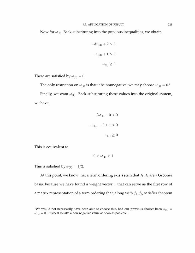
9.3. APPLICATION OF RESULT 221
Now for ω(3). Back-substituting into the previous inequalities, we obtain
−3ω(3) + 2 > 0
−ω(3) + 1 > 0
ω(3) ≥ 0
These are satisfied by ω(3) = 0.
The only restriction on ω(2) is that it be nonnegative; we may choose ω(1) = 0.1
Finally, we want ω(1). Back-substituting these values into the original system,
we have
2ω(1) − 0 > 0
−ω(1) − 0 + 1 > 0
ω(1) ≥ 0
This is equivalent to
0 < ω(1) < 1
This is satisfied by ω(1) = 1/2.
At this point, we know that a term ordering exists such that f1, f2 are a Gröbner
basis, because we have found a weight vector ω that can serve as the first row of
a matrix representation of a term ordering that, along with f1, f2, satisfies theorem
1We would not necessarily have been able to choose this, had our previous choices been ω(3) =ω(4) = 0. It is best to take a non-negative value as soon as possible.
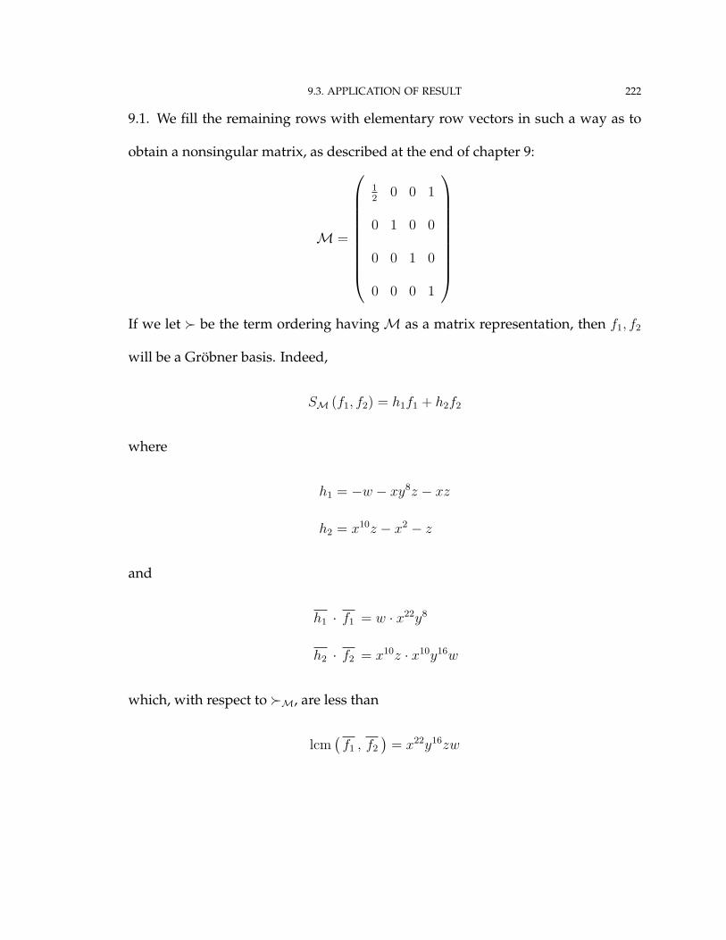
9.3. APPLICATION OF RESULT 222
9.1. We fill the remaining rows with elementary row vectors in such a way as to
obtain a nonsingular matrix, as described at the end of chapter 9:
M =
12
0 0 1
0 1 0 0
0 0 1 0
0 0 0 1
If we let � be the term ordering havingM as a matrix representation, then f1, f2
will be a Gröbner basis. Indeed,
SM (f1, f2) = h1f1 + h2f2
where
h1 = −w − xy8z − xz
h2 = x10z − x2 − z
and
h1 · f1 = w · x22y8
h2 · f2 = x10z · x10y16w
which, with respect to �M, are less than
lcm(f1 , f2
)= x22y16zw
9.3. APPLICATION OF RESULT 223
(This becomes clear from comparing their weights with respect to the first row of
M.) Notice that the representation corresponds to the trailing terms of c1, c2, which
is consistent with the proof of 2.4. (The reader will recall that theorem 2.4 is used
in the proof of theorem 9.1.) �
Computing a Gröbner basis for f1, f2 of example 9.5 with Maple using either
the term orderings tdeg (x, y, z, w) or plex (x, y, z, w) gives us a set of 13 or 14 poly-
nomials (it depends on the polynomial). Different permutations of the variables
gives us smaller sets; some give a set of only 2 polynomials. However, there is no
clear way to guess which permutation of the variables gives us a “small” Gröbner
basis, apart from the algorithm that we have described.
9.3.3. EXPERIMENTAL RESULTS. We conducted two kinds of tests: unstructured
and structured.
UNSTRUCTURED TESTS. For these tests we ran the algorithm on randomly-gene-
rated polynomials. We timed the algorithm and kept track of how many times we
detected a Gröbner basis. We ran three different tests, varying both the number of
terms, the total degree of each term, and the number of indeterminates.
All the random polynomials had the following features in common:
• coefficients were random, over −99 . . . 99
• exponents for indeterminates were random, over 0 . . . 5

9.3. APPLICATION OF RESULT 224
Table 9.1: Number of times we detected a Gröbner basis for f1, f2 (six terms of totaldegree six).
# vars # pairs # detections time per test2 1000 80 .10s3 1000 275 .23s4 1000 489 .48s5 1000 670 .76s6 1000 800 0.98s7 1000 889 1.43s
This leaves it to the experiment to specify the number of indeterminates, the num-
ber of terms, and their total degree, and we experimented with each of these val-
ues.
For the data in table 9.1, we kept the number of terms and the total degree
fixed, varying only the number of indeterminates. As the number increases, the
number of detections skyrocket. By the time we reach n = 7 indeterminates, we are
detecting a Gröbner basis for the vast majority of the generated polynomials. Why?
Maple’s randpoly() appears to generate terms in such a way as to favor single-
indeterminate terms when the total degree is not much higher than the maximum
power of an indeterminate. The resulting polynomials have a large number of
terms in only one indeterminate, so that the polynomials are prime. It is unlikely
that a corresponding percentage of real-world polynomial systems would look like
this, since most real-world problems have some sort of structure; nevertheless, the
data give us some idea about the possibility for success in these cases.

9.3. APPLICATION OF RESULT 225
Table 9.2: Number of times we detected a Gröbner basis for f1, f2 (10% sparse,total degree 6).
# vars # pairs # detections time per test2 1000 159 .05s3 1000 296 .41s4 1000 569 7.50s5 1000 855 94.83s
The data of table 9.2 varied the number of terms, while keeping the total degree
constant. The number of terms was kept at 10% sparsity, by which we mean
(9.3) .1×
# vars + degree
degree
With the total degree fixed at six, this gives us three terms for n = 2 variables, nine
terms for n = 3, twenty-one terms for n = 4, and forty-six terms for n = 5. We did
not proceed beyond n = 5 since at that point it was taking a long time to complete
the tests (94.83 seconds on average).
Despite the increased number of terms, the number of detections continues to
skyrocket; in fact, we find even more detections for a given n than in table 9.1. We
believe that this is due to the fixed low total degree of each polynomial (later data
will bear this out). It is useful to observe how the time per test also skyrocketed.
Since most randomly-generated polynomials will be relatively prime, we believe
that this increase in time is due to the increased complexity of solving the associ-
ated system of linear inequalities (there are more than 80 inequalities for n = 5).

9.3. APPLICATION OF RESULT 226
Table 9.3: Number of times we detected a Gröbner basis for f1, f2 (six terms of totaldegree 6×#vars).
# vars # pairs # detections avg time per test (s)2 1000 45 .063 1000 56 .094 1000 32 .095 1000 21 .086 1000 3 .097 1000 0 .11
Figure 9.1: Summary of the number of detections of Gröbner bases for differentcases of unstructured systems.
For the data in table 9.3, we fixed the number of terms again, but varied their
total degree. Without the low value for the total degree, the number of detected
Gröbner bases plummets not merely from the heights of tables 9.1 and 9.2, but to
the point where we no longer detect any Gröbner bases for n = 7. This is because
Maple’s randpoly() function is much less likely to generate terms of one variable

9.3. APPLICATION OF RESULT 227
Table 9.4: Number of times we detected a Gröbner basis for gc1, gc2 (three terms ineach of g, c1, c2; maximum degree per term is 10).
# vars # pairs # detections average time per test2 1000 127 0.0004183 1000 189 0.0100914 1000 269 0.0238305 1000 265 0.0489706 1000 251 0.1005457 1000 239 0.158870
with the increased total degree. Correspondingly, the average time per test grows
very slowly.
STRUCTURED TESTS. Erich Kaltofen suggested the following tests. Since we know
that the algorithm works for pairs of polynomials that have a common divisor,
and since it is unlikely that we will generate many such polynomials using the
randpoly() function, we can generate three random polynomials g, c1, c2, then
expand f1 = c1g, f2 = c2g, and try the algorithm on these. All the polynomials had
these features in common:
• random coefficients, range −99 . . . 99
• random power on each variable, range 0 . . . 5
This leaves the number of indeterminates, the number of terms, and the maximum
degree per term free for the experiment.
For the data in table 9.4, we kept the number of terms of g, c1, c2 fixed at three,
and the maximum degree per term fixed at ten. Once again we find the number
of detections increasing as we increase the number of variables. Again, we expect

9.3. APPLICATION OF RESULT 228
Table 9.5: Number of times we detected a Gröbner basis for gc1, gc2 (number ofterms in each of g, c1, c2 fixed at 5% sparsity, minimum two terms for c1, c2; maxi-mum degree per term is 10).
# vars # pairs # detections average time per test2 1000 237 0.0285503 1000 344 0.0411504 1000 350 0.0501205 1000 340 0.0774906 1000 331 0.0710007 1000 283 0.075450
that this is due to the fixed total degree. We find that the number of detections
does not vary so much as for the unstructured polynomials: from a low of 13%, we
reach a plateau of 30%, compared to a low of 8% and a high of 89% in table 9.4.
Of course, the data of table 9.4 are not entirely comparable to previous tests.
This is due to differences in the polynomials generated; for example, the polyno-
mials in the unstructured case were almost always relatively prime, whereas the
polynomials in the structured case are never relatively prime. Also, we might not
always have six terms in each of f1, f2; we would expect fewer terms on occasion,
due to simplification.
For table 9.5, we kept the maximum degree of the polynomials fixed, while
increasing the number of terms of g, c1, c2 to reflect a sparsity of 5%. We used the
formula of equation (9.3) on page 225. For a low number of variables, however,
this meant that f1, f2 were always monomials; to avoid that, we restricted c1, c2 to
a minimum of two terms.
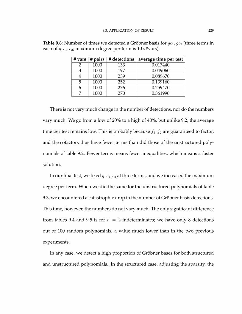
9.3. APPLICATION OF RESULT 229
Table 9.6: Number of times we detected a Gröbner basis for gc1, gc2 (three terms ineach of g, c1, c2; maximum degree per term is 10×#vars).
# vars # pairs # detections average time per test2 1000 133 0.0174403 1000 197 0.0490604 1000 239 0.0896705 1000 252 0.1391606 1000 276 0.2594707 1000 270 0.361990
There is not very much change in the number of detections, nor do the numbers
vary much. We go from a low of 20% to a high of 40%, but unlike 9.2, the average
time per test remains low. This is probably because f1, f2 are guaranteed to factor,
and the cofactors thus have fewer terms than did those of the unstructured poly-
nomials of table 9.2. Fewer terms means fewer inequalities, which means a faster
solution.
In our final test, we fixed g, c1, c2 at three terms, and we increased the maximum
degree per term. When we did the same for the unstructured polynomials of table
9.3, we encountered a catastrophic drop in the number of Gröbner basis detections.
This time, however, the numbers do not vary much. The only significant difference
from tables 9.4 and 9.5 is for n = 2 indeterminates; we have only 8 detections
out of 100 random polynomials, a value much lower than in the two previous
experiments.
In any case, we detect a high proportion of Gröbner bases for both structured
and unstructured polynomials. In the structured case, adjusting the sparsity, the
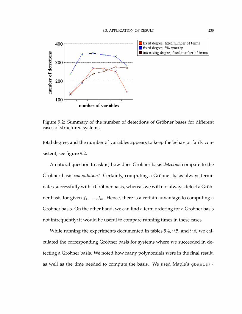
9.3. APPLICATION OF RESULT 230
Figure 9.2: Summary of the number of detections of Gröbner bases for differentcases of structured systems.
total degree, and the number of variables appears to keep the behavior fairly con-
sistent; see figure 9.2.
A natural question to ask is, how does Gröbner basis detection compare to the
Gröbner basis computation? Certainly, computing a Gröbner basis always termi-
nates successfully with a Gröbner basis, whereas we will not always detect a Gröb-
ner basis for given f1, . . . , fm. Hence, there is a certain advantage to computing a
Gröbner basis. On the other hand, we can find a term ordering for a Gröbner basis
not infrequently; it would be useful to compare running times in these cases.
While running the experiments documented in tables 9.4, 9.5, and 9.6, we cal-
culated the corresponding Gröbner basis for systems where we succeeded in de-
tecting a Gröbner basis. We noted how many polynomials were in the final result,
as well as the time needed to compute the basis. We used Maple’s gbasis()

9.3. APPLICATION OF RESULT 231
Table 9.7: Detection compared to computation: fixed number of terms and fixedtotal degree.
# vars time to detect time to compute size of GB avg size of GB2 0.000418 .025260 2..9 2.83 0.010091 3.329418 2..21 5.24 0.023830 5.494907 2..40 5.95 0.048970 5.565019 2..48 6.06 0.100545 .612988 2..41 6.67 0.158870 .515607 2..28 5.9
Figure 9.3: Detection compared to computation (chart of times): fixed number ofterms and fixed total degree.
command to compute the basis with respect to the total degree term ordering; the
general opinion of most researchers is that this ordering gives very good perfor-
mance when computing a Gröbner basis (see also [Tra05]). We present the data in
tables 9.7, 9.8, and 9.9. With only one exception, it always takes longer – and
usually much longer – to compute the Gröbner basis than to detect it. The average

9.3. APPLICATION OF RESULT 232
Table 9.8: Detection compared to computation: fixed sparsity of terms and fixedtotal degree.
# vars time to detect time to compute size of GB avg size of GB2 0.028550 .024430 1..5 2.53 0.041150 .058634 2..14 3.84 0.050120 .105714 2..18 4.35 0.077490 .086529 2..23 4.76 0.071000 .134230 1..26 4.57 0.075450 .121625 2..23 4.5
Figure 9.4: Detection compared to computation (chart of times): 5% sparsity ofterms and fixed total degree.
Table 9.9: Detection compared to computation: fixed number of terms and increas-ing total degree.
# vars time to detect time to compute size of GB avg size of GB2 0.017440 .186617 2..9 2.93 0.049060 15.701117 2..25 4.84 0.089670 20.773808 2..59 6.25 0.139160 1.420317 2..43 6.86 0.259470 31.433587 2..37 6.57 0.361990 16.906481 2..34 6.1
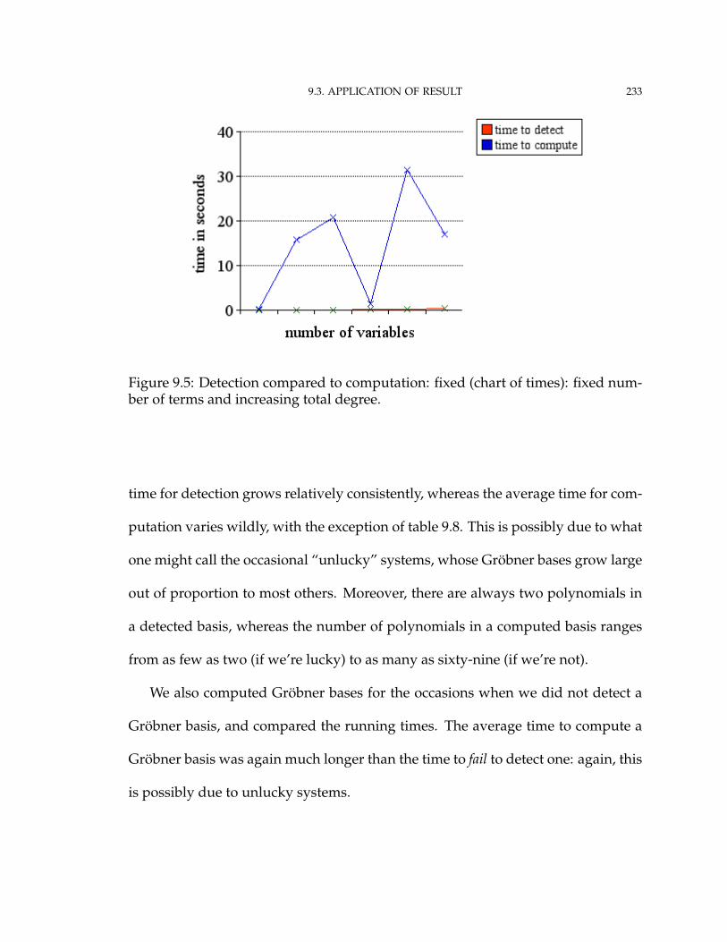
9.3. APPLICATION OF RESULT 233
Figure 9.5: Detection compared to computation: fixed (chart of times): fixed num-ber of terms and increasing total degree.
time for detection grows relatively consistently, whereas the average time for com-
putation varies wildly, with the exception of table 9.8. This is possibly due to what
one might call the occasional “unlucky” systems, whose Gröbner bases grow large
out of proportion to most others. Moreover, there are always two polynomials in
a detected basis, whereas the number of polynomials in a computed basis ranges
from as few as two (if we’re lucky) to as many as sixty-nine (if we’re not).
We also computed Gröbner bases for the occasions when we did not detect a
Gröbner basis, and compared the running times. The average time to compute a
Gröbner basis was again much longer than the time to fail to detect one: again, this
is possibly due to unlucky systems.

9.3. APPLICATION OF RESULT 234
The data suggest that Gröbner basis detection could be a viable starting point
for future optimization of Gröbner basis algorithms. Further research to generalize
the algorithms to a larger number of polynomials could be worthwhile.
Conclusion
We have presented combinatorial criteria that allow us to skip:
• all S-polynomial reductions;
• all but one S-polynomial reductions;
• all but two S-polynomial reductions, for a set of three polynomials
f1, f2, f3.
We also presented a new method for Gröbner basis detection for a set of two poly-
nomials f1, f2.
Directions for future research are clear. First, we have the opportunity to gen-
eralize the combinatorial criteria that allow us to skip all but two S-polynomial
reductions. There are two possible paths:
• for m > 3, find criteria that allow us to skip all but two S-poly-
nomial reductions;
• for m > 3, find criteria that allow us to skip exactly one S-poly-
nomial reduction.
235

CONCLUSION 236
These two paths coincide when m = 3.
I have carried out some research on skipping all but two S-polynomial reduc-
tions for m > 3, but so far I cannot even hazard a guess as to what the solution
might be.
Second, we have the opportunity to generalize the method of Gröbner basis re-
duction to m > 2 polynomials. Originally, I believed that this would be based on
combinatorial criteria, just as theorem 9.1 on page 209 depends on Buchberger’s
first criterion. For a while, I believed that the solution embodied in theorem 6.3 on
page 124 (the new combinatorial criterion) would help formulate a characteriza-
tion of Gröbner bases consisting of three polynomials. Subsequent research has
revealed that this is not the case, so we are back at square one.
Third, we have the opportunity to implement the method of Gritzmann and
Sturmfels, and compare its performance on sets of two polynomials to the method
we lay out in chapter 9. This will require the use of a computational package that
can efficiently compute Minkowski sums of polytopes and their polyhedra, as well
as pick representative weight vectors from the normal cones of the vertices of a
polyhedron. The Convex package [Fra04] is a possible candidate; however, the
documentation indicates that its implementation of Minkowski sums is “trivial,
hence slow.” I expect that I will have to spend some time researching ways to
optimize this code and contribute to this project – or else, find a different package.
Bibliography
[BS87] Dave Bayer and Mike Stillman, A criterion for detecting m-regularity, Inventiones Mathe-
maticae 87 (1987), no. 1, 1–11.
[Buc65] Bruno Buchberger, Ein Algorithmus zum Auffinden der Basiselemente des Restklassenringes
nach einem nulldimensionalem Polynomideal (an algorithm for finding the basis elements in the
residue class ring modulo a zero dimensional polynomial ideal), Ph.D. thesis, Mathematical
Insitute, University of Innsbruck, Austria, 1965, English translation to appear in the
Journal of Symbolic Computation.
[Buc79] , A criterion for detecting unnecessary reductions in the construction of Gröbner bases,
Proceedings of the EUROSAM 79 Symposium on Symbolic and Algebraic Manipula-
tion, Marseille, June 26-28, 1979 (Berlin - Heidelberg - New York) (E. W. Ng, ed.), Lecture
Notes in Computer Science, vol. 72, Springer, 1979, pp. 3–21.
[BWK93] Thomas Becker, Volker Weispfenning, and Hans Kredel, Gröbner bases: a computational
approach to commutative algebra, Springer-Verlag New York, Inc., New York, 1993.
[CKM97] Stéphane Collart, Michael Kalkbrenner, and Daniel Mall, Converting bases with the Gröb-
ner walk, Journal of Symbolic Computation 24 (1997), no. 3–4, 465–469.
237
BIBLIOGRAPHY 238
[CKR02] Massimo Caboara, Martin Kreuzer, and Lorenzo Robbiano, Minimal sets of critical pairs,
Proceedings of the First Congress of Mathematical Software (B. Cohen, X. Gao, and
N. Takayama, eds.), World Scientific, 2002, pp. 390–404.
[CLO97] David Cox, John Little, and Donal O’Shea, Ideals, varieties, and algorithms, second ed.,
Springer-Verlag New York, Inc., New York, 1997.
[CLO98] , Using algebraic geometry, Springer-Verlag New York, Inc., New York, 1998.
[Coh03] Joel Cohen, Computer algebra and symbolic computation: Mathematical methods, A K Peters,
Ltd., Natick, MA, 2003.
[Eis95] David Eisenbud, Commutative algebra with a view toward algebraic geometry, Springer-
Verlag New York, Inc., New York, 1995.
[Fau99] Jean-Charles Faugère, A new efficient algorithm for computing Gröbner bases (F4), Journal
of Pure and Applied Algebra 139 (1999), no. 1-3, 61–88.
[Fau02] , A new efficient algorithm for computing Gröbner bases without reduction to zero F5,
International Symposium on Symbolic and Algebraic Computation Symposium - IS-
SAC 2002, Villeneuve d’Ascq, France, Jul 2002.
[FGLM93] Jean-Charles Faugère, Patrizia Gianni, Daniel Lazard, and Teo Mora, Efficient computa-
tion of zero-dimensional Gröbner bases by change of ordering, Journal of Symbolic Computa-
tion 16 (1993), no. 4, 329–344.
[Fra04] Matthias Franz, Convex: a Maple package for convex ge-
ometry, version 1.1, 2004, Maple worksheet available at
http://www-fourier.ujf-grenoble.fr/~franz/convex/ .
[GM88] Rudiger Gebauer and Hans Möller, On an installation of Buchberger’s algorithm, Journal
of Symbolic Computation 6 (1988), 275–286.

BIBLIOGRAPHY 239
[GS93] Peter Gritzmann and Bernd Sturmfels, Minkowski addition of polytopes: Computational
complexity and applications to Gröbner bases, SIAM J. Disc. Math 6 (1993), no. 2, 246–269.
[Hon98] Hoon Hong, Gröbner basis under composition I, Journal of Symbolic Computation 25
(1998), 643–663.
[HP04] Hoon Hong and John Perry, Gröbner basis detection, 2004, Maple worksheet available at
http://www4.ncsu.edu/~jeperry/Research/GBDetection.mw .
[HW99] Hoon Hong and Volker Weispfenning, Algorithmic theory of admissible term orders, avail-
able at http://www.math.ncsu.edu/~hong/ , 1999.
[KR00] Martin Kreuzer and Lorenzo Robbiano, Computational commutative algebra I, Springer-
Verlag, Heidelberg, 2000.
[MR88] Teo Mora and Lorenzo Robbiano, The Gröbner fan of an ideal, Journal of Symbolic Com-
putation 6 (1988), 183–208.
[Per94] John Perry, GraphDQ, 1994, binary code (AmigaOS) available at
http://wuarchive.wustl.edu/aminet/misc/math/graphdq.lha .
[Rob86] Lorenzo Robbiano, On the theory of graded structures, Journal of Symbolic Computation
2 (1986), 139–170.
[SW97] Bernd Sturmfels and Markus Wiegelmann, Structural Gröbner basis detection, Applicable
Algebra in Engineering, Communication and Computing 8 (1997), 257–263.
[Tra05] Quoc-Nam Tran, Ideal-specified term orders for elimination and applications in implicitiza-
tion, Proceedings of the Tenth International Conference on Applications of Computer
Algebra (Beaumont, TX), International Scientific Committee for Applications of Com-
puter Algebra, 2005, Selected papers to appear in a forthcoming issue of the Journal of
Symbolic Computation, pp. 15–24.
BIBLIOGRAPHY 240
[vzGG99] Joachim von zur Gathen and Jurgen Gerhard, Modern computer algebra, Cambridge Uni-
versity Press, Cambridge, 1999.
[Wei87] Volker Weispfenning, Admissible orderings and linear forms, ACM SIGSAM Bulletin 21
(1987), no. 2, 16–18.
[Woo04] Chi Woo, Planetmath.org, 2004, online encyclopedia article available at
http://planetmath.org/encyclopedia/Indeterminate.html .
Index
admissible matrix, 172
equivalence, 187
of �, 174
algorithms
Can_Skip_All_But_One_SPolys, 110
Can_Skip_All_SPolys, 90
Can_Skip_Third_Spoly, 148
Exists_Tord_with_given_leadterms, 215
GB_Detection_by_Minkowski_Sums, 208
Implied_GB, 58
Is_GB, 35
Tord_for_GB, 214
Buchberger’s criteria
allow us to skip S-polynomial reduction,
59
first criterion, 59, 69
term diagram, 74
second criterion, 62, 69
does not guarantee reduction to zero, 68
term diagram, 75
variablewise, 123
coefficient, 8
leading coefficient, 12
combinatorial criterion, 58
Buchberger’s criteria, see Buchberger’s
criteria
complete, 80
existence of non-Buchberger criteria, 149
exponent vectors, 172
Gröbner basis, 19
equivalent conditions, 34
Gröbner basis detection, 168
241
INDEX 242
indeterminate, 8
leading coefficient, 12
leading monomial, 12
leading term, 12
lex term ordering, 11
Minkowski sum, 203
monomial, 8
leading monomial, 12
Newton polyhedron, 202
Newton polytope, 201
normal cone, 204
reduction, 16
implies representation, 30
relationship with representation, 29–31
representation
does not imply reduction, 31
relationship with reduction, 29–31
representation of an S-polynomial, 28
S-polynomial
parallel with Gaussian elimination, 24
Skipping S-polynomial reduction
not equivalent to reduction to zero, 57
skipping S-polynomial reduction, 55
allowed by Buchberger’s criteria, 59
experimental results, 117
theorems, 87, 102, 124
tdeg term ordering, 14
term, 8
leading term, 12
term diagrams, 71, 75
Buchberger’s first criterion, 74
locating greatest common divisor and least
common multiple, 73
shading for divisible terms, 73
term ordering, 9
admissible, 9
as shorthand for admissible term ordering,
9
equivalence, 206
lexicographic, 11
properties, 15
total-degree, 14

INDEX 243
variable, 8
weight, 174


![[ ABSTRACT ]](https://img.dokumen.tips/doc/110x75/56814589550346895db26fcc/-abstract--56956c8cc7359.jpg)
