Abstract

This work presents an improved variant of the Direct Torque Control (DTC) for aPermanent Magnet Synchronous Motor (PMSM). The improved DTC use a highernumber of voltage space vectors by introducing a kind of Space Vector Modulationtechnique. The higher number of space vectors are tabulated in more precise switch tableswhich also take the emf induced in the stator windings into account. The emf voltagesignificantly affect the motor behavior from a given space vector. It is discussed how theswitch tables are constructed. Experiments from the classical and improved DTC arecompared and show that the torque, flux linkage and stator current ripples aresignificantly decreased with the improved DTC.

1

Acknowledgment

I have worked on this thesis at the Universitat Politècnica de Catalunya in Terrassa in theMotion Control and Industrial Applications Group from October 2004 until March 2005.I would like to say thanks to my supervisor in Barcelona, Dr. Luis Romeral and otherpeople in the UPC who helped me during this work. Also I would like to thank KarlHenrik Johansson at S3, KTH.

Stockholm, May 2005David Ocen

2

Contents

I Introduction 5

Chapter 1 Permanent Magnet Synchronous Motor 61.1 Derivation of motor equations, abc-frame 61.2 Transformation to qdØ-frame 14

Chapter 2 Some common control schemes for PM motors 202.1. Scalar control 202.2. Vector control 21

Chapter 3 Direct Torque Control 253.1 The Direct Torque Control system 263.2 Torque and Flux equations 313.3 System analysis 373.4 Some problems with the DTC system 41

Chapter 4 Discrete Space Vector Modulation 444.1 Introduction to the DSVM – DTC system 444.2 Space vector selection 47

Chapter 5 Simulation and experimental results 50

Chapter 6 Conclusion 55

References 58

Appendix 61I. Motor parameters

3

Notations

δ load angleid d-axis currentiq q-axis currentis current vector value, ║iqd║Ks Park Transformλd d-axis fluxλq q-axis fluxλs flux vector value, ║Λqd║Ld d-axis inductanceLq q-axis inductanceLM q and d-axis inductance, used when Lq = Ld = LM

Ls stator windings self and mutual inductance matrixθm rotor position, mechanical angleθr rotor position, electrical angleωm angular velocity, mechanical angleωr angular velocity, electrical angleP number of magnetic poles, two for each magnetℜ magnetic reluctanceRs, rs stator winding resistancevabc stator winding voltage vectorvd d-axis voltagevq q-axis voltagevs emf/speed-voltage, ωrλs

CSI Current Source InverterDTC Direct Torque ControlFOC Field Oriented ControlSVM Space Vector ModulationVSI Voltage Source InverterPMSM Permanent Magnet Synchronous Motor

4

I. Introduction

Direct Torque Control was introduced in the 1980´s for Induction Motors as a newapproach for torque and flux control. Direct Torque Control (DTC) directly controls theinverter states based on the errors between the reference and estimated values of torqueand flux. It selects one of six voltage vectors generated by a Voltage Source Inverter tokeep torque and flux within the limits of two hysteresis bands.Characteristics of DTC are:

• good dynamic torque response• robustness• low complexity

The main drawback of the DTC is its relatively high torque and flux ripple.In this work a background is presented in chapter 1 and 2. Chapter 1 derives the motormodel equations used for simulations with Simulink. Chapter 2 presents some commoncontrol techniques used for control of Permanent Magnet Synchronous Motors (PMSM).The classical DTC scheme is presented and analyzed in chapter 3. In chapter 4 one of theimproved DTC schemes proposed in the research literature is presented and comparedwith the classical. The improved scheme is called Discrete Space Vector Modulation(DSVM) – DTC, and address the problem with torque ripple in the basic DTC system.In chapter 5 simulation and experimental results are presented and compared. Bothsystems are modeled in Simulink and then tested on a dSPACE platform for theexperimental results.

5

Chapter 1 Permanent Magnet Synchronous Motor

In this chapter the motor model used for simulations is derived. The model focuses on thefundamental frequency component. The magnetic circuits are assumed linear, statorwindings are considered sinusoidally distributed and the magnetic fields are assumedequal along the rotor axis, so no end fringing effects are taken into account.The model can be found in [4,8], but is also found in most papers and books treating thePM synchronous motor.

1.1 Derivation of motor equations, abc-frame

The Permanent Magnet Synchronous Motor is a three-phase AC machine. The windingsare Y-connected and displaced 120 electrical degrees in space.

Figure 1.1, A simplified sketch of a PM motor showing stator windings, rotor magnet and their magnetic axes

The stator windings consists of individual coils connected and wound in different slotsso as to approximate a sinusoidal distribution, to minimize the space harmonics [5]. InFigure 1.1 the stator windings are depicted as single coils together with their resultantmagnetic axes.

The material of which the rotor and stator are made of has a lower reluctance than the air-gap between them, and therefore almost all the magnetic fields are concentrated to the air-gap. Hence, one can ignore the magnetic reluctance in the stator and rotor and assume allmagnetic energy is in the air-gap. Also, because the air-gap is short in comparison to theradius of the rotor, one can assume the fields are constant across the air-gap. The fieldsare supposed radially directed because they tend to choose the lowest reluctance path.

Figure 1.2 shows the magnetic field of a concentrated winding.

6

Figure 1.2, B-field of a concentrated winding that spans π radians

When a stator winding is distributed over several slots the resultant field more resemblesa sine wave. Figure 1.3 shows a distributed winding and the fundamental component ofthe magnetic field.

Figure 1.3, Magnetic field of a distributed windingand its fundamental frequency component

Magneto Motive Force

Consider the integral mmf = ∫H·dl [A], where the integral path is across one air-gap. If weevaluate Vm = ∮H⋅dl along the integral path shown in figure 1.4 and keep in mind thatthe magnetic field was confined to the air-gap gives, Vm = 2∫H·dl, since both air-gapscontribute equally to the integral.

Figure 1.4, Integral path for Vm = ∮H⋅dl

If the winding is sinusoidally distributed then Vm = NIcos(φ), so that mmf = NI/2 cos(φ).

7

φ is measured from winding a's magnetic axis.Mmf for windings b and c are similar, the difference is a space-phase delay by 2π/3 and4π/3 radians respectively,

mmf a=N I2

cosφ (1.1)

mmf b=N I2

cosφ−2/3 (1.2)

mmf c=N I2

cosφ2/3 (1.3)

Rotating mmf wave

When the three stator windings are displaced in space by 2π/3 electrical radians and fedby a balanced set of sinusoidal voltages the result is a single rotating mmf wave with thesame frequency and with amplitude 3/2 times that of each winding.For phase a the time dependent mmf wave can be written

F a=F max cos θ cosωt , (1.4)

where θ is measured from a's magnetic axis.Using the equality

cos acos b=12

cosa−b12

cosab , (1.5)

one may rewrite Fa as

F a=F max 12

cosθ−ωt 12

cosθωt . (1.6)

This is the superposition of two rotating waves; Fa+ = ½ Fmax cos(θ – ωt) in the positive

or counterclockwise direction and Fa- = ½ Fmax cos(θ + ωt) in the negative direction.

Windings b and c are phase delayed 2π/3 and 4π/3 respectively both in space and timephase which results in the following expressions,

F b=F b+F b

-=F max 12

cosθ−ωt 12

cosθωt2/3 (1.7)

F c=F c+F c

-=F max 12

cosθ−ωt 12

cos θωt−2/3 . (1.8)

Summing the positive and negative mmf waves individually gives

8

F a+F b

+F c+=3

2F max cosθ−ωt (1.9)

andF a

-F b-F c

-=0 . (1.10)

Hence the resultant wave, F, is

F=32

F max cosθ – ωt . (1.11)

PMSM motor equations

In a motor with more than one magnet the electrical angular velocity differ from themechanical. Their relationship is

θ r=P2

θm , (1.12)

where θr is the rotor position measured in electrical degrees, θm in mechanical degrees andP is the number of poles (two for each magnet).

The voltage, v, over each stator winding is the sum of the resistive voltage drop, ri, andthe voltage induced from the time varying flux linkage, dλ/dt,

va=ra iaddt

λa

vb=rb ibddt

λb (1.13)

vc=rc icddt

λc .

The stator windings are wound with the same number of turns so the resistance is equal inall three windings, ra = rb = rc = rs.In matrix form these voltage equations (1.13) becomes,

V abc=Rs iabcddtΛabc=[r s 0 0

0 r s 00 0 r s

][ia

ib

ic] d

dt [a

b

c] (1.14)

Flux linkage in a linear magnetic circuit is the product of inductance and current. Themotor model was assumed linear, which is a fairly accurate approximation if saturation

9

does not occur.Hence,

Λabc=Ls iabcλm , (1.15)

where Ls contains self and mutual inductances and λm is the flux through the statorwindings due to the permanent magnet.

Inductance matrix Ls

Ls=[Laa Lab Lac

Lab Lbb Lbc

Lac Lbc Lcc] (1.16)

The diagonal elements in the inductance matrix Ls are self inductances and the offdiagonal elements are mutual inductances. The matrix is symmetric because the fluxcoupling between two windings is equal in both directions.A current in a stator winding gives rise to a leakage flux and a magnetizing flux. Themagnetizing flux is confined to the air-gap and give rise to the rotating mmf wave.Leakage flux is assumed to only affect its own winding. In a magnetically linear circuitself inductance is the ratio of the flux flowing through the winding to the current flowingin the winding with all other currents set to zero.Let the self inductance be Laa = Lls + Lm, where Lls is the leakage inductance and Lm themagnetizing inductance. Now the magnetizing inductance is generally not constant; reluctance may depend onrotor position. For example the, unrealistic, rotor depicted in Figure 1.1 would have had alower reluctance path along its d-axis because iron has lower reluctance than air.This phenomenon is called saliency and is present in some permanent magnet motors,especially those with a high number of pole pairs.

Let Laa = Lls + Lmq when the rotor quadrature axis is parallel with magnetic axis a, and Laa = Lls + Lmd when the direct axis is.

The magnetic field from the rotor magnet has a preferred direction along the direct axis.Reluctance is therefore lower along the d-axis, ℜd < ℜq. An inductance may be expressedas L = N2/ℜ, which implies that

LmqLmd . (1.17)

Thus,

LlsLmq ≤ Laa ≤ LlsLmd (1.18)

10

Laa varies periodically with twice the speed of the rotor since when the rotor has rotated πradians the same magnetic characteristics are restored. (It is only the varying reluctancepath which is considered here, the PM flux is considered later).The min values of Laa occurs at

θ r=0, , 2 , ...

and maximum values at

θ r=2

,32

, ...

Assume Laa(θr) varies sinusoidally, then

Laa=LlsL−LΔ cos2θ r , (1.19)

where L is the average value of the magnetizing inductance and LΔ half the amplitude ofthe sinusoidal varying magnetizing inductance.

The Lbb and Lcc self inductances can be found from eq. (1.19) by introducing a 2π/3 and4π/3 radians space-phase lag respectively

Lbb=LlsL−LΔ cos 2θ r−2/3=LlsL−LΔ cos 2θ r2/3 (1.20)

Lcc=LlsL−LΔ cos 2θ r−4/3=LlsL−LΔ cos2θ r−2/3 (1.21)

Mutual inductance

Assume the mutual inductance is only due to the space mmf wave. Inductance wasassumed to vary sinusoidally around a constant value,

Laa=LlsL−LΔ cos2θ r . (1.22)

Since an inductance may be expressed as L = N2/ℜ, the reluctance for Laa (without theleakage inductance) may be written

ℜ−1=α1−α2 cos 2θ r (1.23)

or by making use of ℜ = l/(μA) the equivalent air-gap length is

l−1θ r=β1−β2 cos2θ r . (1.24)

11

When measured an angle φ from a's magnetic axis

l−1φ−θ r=β1−β2 cos 2φ−2θ r . (1.25)

The flux density with all currents set to zero except ia is

Br=μ mmf a φ l−1φ−θ r=μ

N ia

2cosφ β1−β2 cos 2φ−2θ r . (1.26)

The flux through a winding turn with its magnetic axis at an angle φ from winding a,

ψa=∫−

2

2 Br ,rrl d

=r l μ N ia β1 cosφ−β2/2cos φ−2θ r−cos3φ−2θ r/3(1.27)

To obtain the flux coupling from winding a through winding b, the flux linked from eachturn must be summed over the whole winding,

λab=∫N ba ,rd . (1.28)

b's winding distribution is

N b=N2

cos −23

(1.29)

which after some calculation leads to

λab=∫b−

2

b2 N ba ,rd

=rl N2

2

ia−1

2−2

2cos2r−

23

(1.30)

The mutual inductance Lab is obtained by dividing by ia. To express this equation in thesame form as the other inductances, compare it with the self inductance for winding a

Laa=Llsrl N2

2

1−2

2cos 2r (1.31)

which gives

12

Lab=−L /2−LΔ cos 2θ r−2/3 . (1.32)

The mutual inductances Lac and Lbc are calculated in a similar way.

Lac=−L /2−LΔ cos2θ r2/3 (1.33)

Lbc=−L /2−LΔ cos2θ r (1.34)

The above derivations lead to the following inductance matrix,

Lsθ r=[ LlsL−Lcos2r − L2−Lcos2r−

23

− L2−Lcos 2r

23

− L2−Lcos 2r−

23

LlsL−Lcos 2r23

− L2−Lcos2r

− L2−Lcos 2r

23

− L2−Lcos2r LlsL−Lcos2r−

23

] .

(1.35)

With this inductance matrix the machine flux originating from the stator currents is, Lsiabc.

Permanent Magnet

The flux linkage from the permanent magnet is

λm=m[sin r

sin r−23

sin r23

] . (1.36)

Mechanical equation

Both the inductance matrix and the permanent magnet flux linkage depend on rotorposition. Therefore, the mechanical equations of the rotor must be included in the motormodel to have a complete description of the motor.

Using Newton's law

Jd ωm

dt=T e−T L , (1.37)

where J is the inertia of the rotor plus load, Te the motor torque, TL load torque and

13

ωm = dθm/dt. Torque is change in energy per change in angle, thus, using the coenergy [8]

W c=12iabc

T Ls iabciabcT λmW pm , (1.38)

the torque produced by the machine is

T e=dW c

dθm. (1.39)

The evaluation will be postponed.

1.2 Transformation to qdØ-frame

Now there is a set of equations which describe the motor. These equations though,depend on rotor position and make the equation system quite involved to solve.If the variables are transformed into a reference frame rotating with the rotor, inductancewill no longer depend on rotor position. This is because in a reference frame attached tothe rotor, reluctance which, in the abc-frame, depends on rotor position will be constant.The transformation used is called the Park Transform.

Let Ks be the Park transform.

[ S q

S d

S∅]=K s[S a

S b

S c] , (1.40)

where S represents voltage, current, etc. in the respective domains. q, d and Ø, stands forquadrature, direct and zero-sequence variables, respectively.

Ks is defined as

K s ≡ 23[cos cos−

23

cos23

sin sin −23

sin 23

12

12

12

] , (1.41)

and its inverse as

14

K s−1=[ cos sin 1

cos −23

sin −23

1

cos 23

sin −23

1] . (1.42)

In Ks there is a factor of 2/3 in front of the matrix. This factor can be understood by thediscussion about the mmf-wave. For a balanced set of, say, voltages, the resultant voltagevector has amplitude 3/2 times that of the individual amplitudes. The factor 2/3 makes theamplitude of quantities expressed in the qd-frame correspond to that of each individualphase in the stator abc-frame.The last row in Ks is the zero sequence. If we consider current and the neutral point of themotor is grounded, then iØ is the current flowing from neutral to ground. Normally motorsare operated with the neutral point floating and so, there is no need to consider the zerosequence.Another feature that may be noted with the above definition of the Park Transform, it isnot power invariant. This is because det(Ks) ≠ 1.

Let

PqdØ=⟨vqdØ , iqdØ⟩=w1 vq iqw2 vd idw3 vØ iØ (1.43)

The input power in the abc-frame is

Pabc=vabc⋅iabc=vabcT iabc . (1.44)

Transform the abc-variables to the qdØ-frame and use the fact that power must be equalin both reference frames,

Pabc=vabcT iabc=K s

−1vqdØT K s

−1 iqdØ=vqdØ K s−T K s

−1 iqdØ

=vqdØ[ 32

0 0

0 32

0

0 0 3]iqdØ=

32 vq iqvd id2 vØ iØ =PqdØ

. (1.45)

⇒

PqdØ=⟨vqdØ , iqdØ⟩=32

vq iq32

vd id3 vØ iØ (1.46)

We are now going to transform Vabc, first to an arbitrary qdØ reference frame, and then letthis transformation be attached to the rotor.

Express vabc in qdØ-variables,

15

vabc=Rs iabcddtΛabc=RsK s

−1 iqdØddt

K s−1 ΛqdØ , (1.47)

and transform vabc into vqdØ,

vqdØ=K s RsK s−1 iqdØK s

ddt

K s−1 ΛqdØ . (1.48)

The resistance does not change when transformed since,

K sRsK s−1=K s r s I K s

−1=r sK s K s−1=Rs . (1.49)

The second term

K sddt

K s−1 ΛqdØ =K s d

dtK s θT ΛqdØK s

−1 ddtΛqdØ θT ,θ r (1.50)

K s θT ddtK sθT =ωT[ 0 1 0

−1 0 00 0 0] (1.51)

K sddt

K s−1 ΛqdØ=ωT[ d

−q

0 ] ddtΛqdØ (1.52)

Voltage equations in the arbitrary frame

vqdØ=Rs iqdØωT[ d

−q

0 ] ddtΛqdØ (1.53)

Now we want to express flux, ΛqdØ, in component form.First expand Λabc,

Λabc=Ls iabcλm=LsK s−1 iqdØλm (1.54)

⇒ΛqdØ=K s LsK s

−1 iqdØK s λm (1.55)

16

K s Lsθ rK s−1=[Lls

32 L−Lcos 2T−2r −3

2Lsin 2T−2r 0

−32

Lsin 2T−2r Lls32 LLcos2T−2r 0

0 0 Lls]

(1.56)

K sθT λmθ r=λm[−sin T−rcos T−r

0 ] (1.57)

For a single phase machine

Lmq=L−LΔ and Lmd=LLΔ .

For a three phase machine the space mmf wave has amplitude 3/2 times that of eachindividual phase which gives,

Lmq=32L−LΔ and Lmd=

32LLΔ (1.58)

⇒

L=13LmdLmq and LΔ=

13Lmd−Lmq . (1.59)

Flux linkage in qdØ coordinates may therefore be expressed as

ΛqdØ=[LdLq

2−

Ld−Lq

2cos2T−2r −

Ld−Lq

2sin 2T−2r 0

−Ld−Lq

2sin 2T−2r

LdLq

2

Ld−Lq

2cos 2T−2r 0

0 0 Lls

][ iq

id

i∅]m[−sin T−rcosT−r

0 ] ,

(1.60)

where Lq = Lls + Lmq and Ld = Lls + Lmd. θT is the angle which rotates the transformedreference frame and θr the rotor position in electrical radians. This is the flux expressed inthe arbitrary reference frame.

If the reference frame rotates in synchronism with the rotor and both angles have the sameinitial conditions then θT = θr, and total flux in the rotor reference frame becomes,

ΛqdØr =[Lq 0 0

0 Ld 00 0 Lls

][ iqr

idr

i∅r ][ 0

m

0 ] . (1.61)

17

Stator voltage expressed in the rotor qdØ-frame then is,

vqdØr =Rs iqdØ

r ωr[ d

−q

0 ] ddtΛqdØ

r , (1.62)

and in expanded form

vqr

vdr

vØr

=r s pLqiqrωr Ld id

rωr λm

=r s pLd idr −ωr Lq iq

r

=r s pLlsiØr

(1.63)

where p = d/dt.

Now let's return to the torque equation.

W c=12iabc

T Ls iabciabcT λmW pm . (1.64)

T e=dW c

dθm= P

2dWcdθ r

= P2 1

2iabc

T ddθ r

Ls iabciabcT d

dθ rλm (1.65)

making a change of variables, iabc = K-1s iqdØ,

T e=

P2 1

2K s

−1 iqdØT d

dθ rLsK s

−1 iqdØK s−1 iqdØ

T ddθ r

λm= P

2 12iqdØ

T K s−T d

dθ rLs K s

−1 iqdØiqdØT K s

−T ddθ r

λm(1.66)

K s−T θT

ddθ r

Lsθ rK s−1θT =

92[−sin 2T−2r cos 2T−2r 0

cos 2T−2r sin 2T−2r 00 0 0] (1.67)

K s−T θT

ddrλmθ r=

32m[cos T−r

sin T−r0 ] (1.68)

⇒

18

T e=P2 9

4L iqdØ

T [−sin 2T−2r cos 2T−2r 0cos 2T−2r sin 2T−2r 0

0 0 0]iqdØ32m iqdØ

T [cos T−rsin T−r

0 ](1.69)

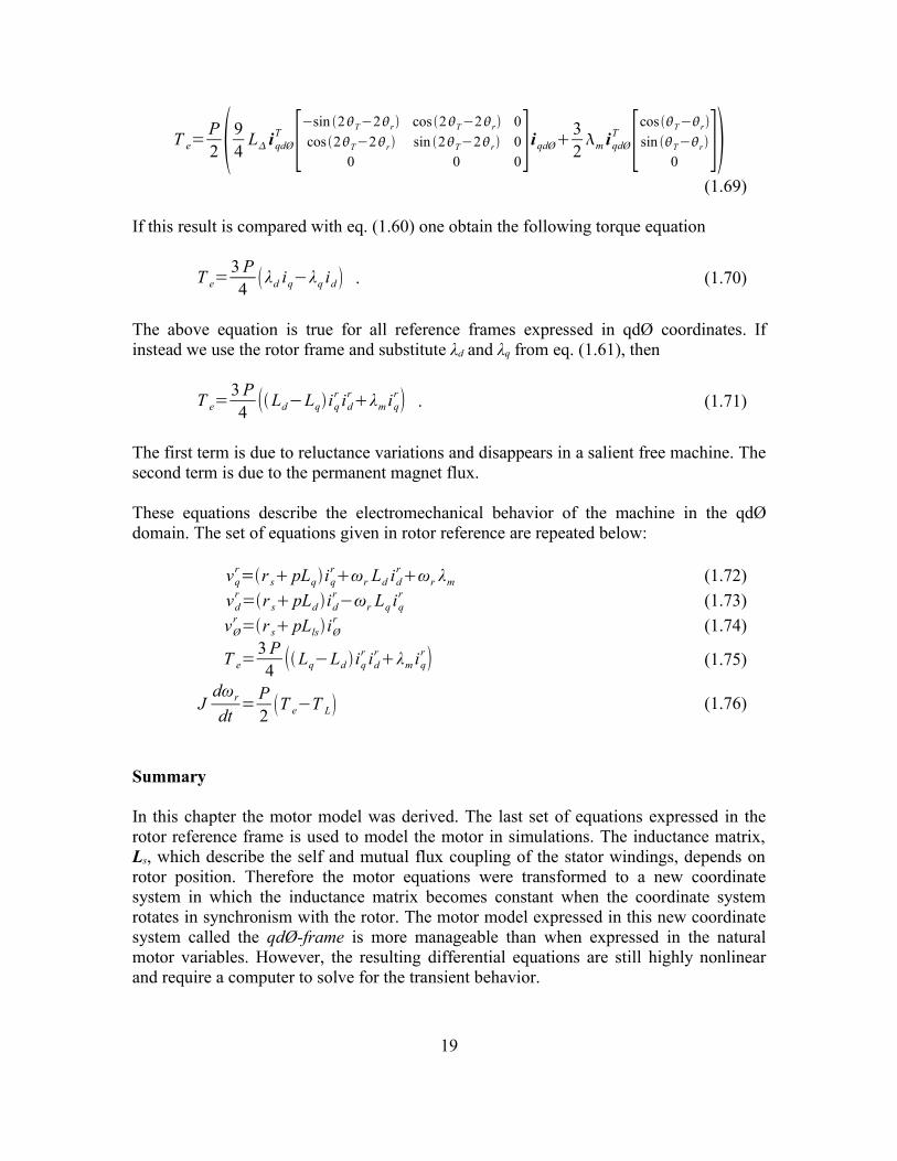
If this result is compared with eq. (1.60) one obtain the following torque equation

T e=3 P4 λd iq−λq id . (1.70)

The above equation is true for all reference frames expressed in qdØ coordinates. Ifinstead we use the rotor frame and substitute λd and λq from eq. (1.61), then

T e=3 P4 Ld−Lqiq

r idrλm iq

r . (1.71)

The first term is due to reluctance variations and disappears in a salient free machine. Thesecond term is due to the permanent magnet flux.

These equations describe the electromechanical behavior of the machine in the qdØdomain. The set of equations given in rotor reference are repeated below:

vqr=r s pLqiq

rωr Ld idrωr λm (1.72)

vdr=r s pLd id

r−ωr Lq iqr (1.73)

vØr =r s pLlsiØ

r (1.74)

T e=3 P4 Lq−Ld iq

r idrλm iq

r (1.75)

Jdωr

dt= P

2 T e−T L (1.76)

Summary

In this chapter the motor model was derived. The last set of equations expressed in therotor reference frame is used to model the motor in simulations. The inductance matrix,Ls, which describe the self and mutual flux coupling of the stator windings, depends onrotor position. Therefore the motor equations were transformed to a new coordinatesystem in which the inductance matrix becomes constant when the coordinate systemrotates in synchronism with the rotor. The motor model expressed in this new coordinatesystem called the qdØ-frame is more manageable than when expressed in the naturalmotor variables. However, the resulting differential equations are still highly nonlinearand require a computer to solve for the transient behavior.

19

Chapter 2 Some common control schemes for PM motors

In this chapter a short summary of some common control techniques used for PM motorcontrol are presented [22]. PMSM control techniques can be divided into scalar andvector control. Scalar control is based on relationships valid in steady-state. Amplitudeand frequency of the controlled variables are considered. In vector control amplitude andposition of a controlled space vector is considered. These relationships are valid evenduring transients which is essential for precise torque and speed control.

Figure 2.1, Some common control techniques used for PMSM.Control methods in the dashed box belong to the DTC family.

2.1 Scalar control

Scalar control is based on relationships valid in steady state. Only magnitude andfrequency of voltage, current, etc. are controlled. Scalar control is used e.g. where severalmotors are driven in parallel by the same inverter.

2.1.1 Volts/Hertz control

Volts/Hertz control is among the simplest control schemes for motor control. The controlis an open-loop scheme and does not use any feedback loops.The idea is to keep stator flux constant at rated value so that the motor develops ratedtorque/ampere ratio over its entire speed range.

The voltage equations for a permanent magnet motor were derived in chapter 1. In qd-coordinates these equations are

vq=r s iqωλdddt

λq (2.1)

20

vd=r s id – ωλqddt

λd (2.2)

where vq and vd are stator voltage, rs stator resistance, i stator current, ω angular velocityand λ is the flux linkage.In stationarity the derivative terms disappears, furthermore, if speed is high the emfvoltage, ωλ, is relatively high and the resistive voltage drop may be ignored.In this case, if stator flux is to be kept constant, the voltage applied should be directlyproportional to the rotor angular frequency.At lower speeds an extra boost voltage is applied to compensate for the resistive drop.The principle is valid only for stationarity when the derivative terms vanish.

2.2 Vector control

The problem with scalar control is that motor flux and torque in general are coupled. Thisinherent coupling affects the response and makes the system prone to instability if it is notconsidered. In vector control, not only the magnitude of the stator and rotor flux isconsidered but also their mutual angle.

2.2.1 Field Oriented Control

The vector control of currents and voltages results in control of the spatial orientation ofthe electromagnetic fields in the machine and has led to the name field orientation.Field Oriented Control usually refers to controllers which maintain a 90º electrical anglebetween rotor and stator field components. Systems which depart from the 90º orientationare referred to as field angle control or angle control [3].

In a DC motor the field flux, which in this case is the stator flux, and the armature flux(rotor) are held orthogonal mechanically by the commutator. When the fields areorthogonal, armature flux does not affect the field flux and the motor torque respondsimmediately to a change in armature flux or equivalently, armature current. In an ACmotor the field flux (which now is in the rotor) rotates, but in a FOC the controller rotatesthe armature (stator) flux so that armature and field flux are kept orthogonal, and hence,the AC motor behaves as a DC motor. The requirements are,

1. Independently controlled armature current to overcome the effects of windingresistance, leakage inductance and induced voltage.

2. Independently controlled or constant field flux.3. Independently controlled orthogonal spatial angle (electrical) between stator and rotor

flux.

A vector controlled PM motor is also known as a brushless DC-machine.

21

To see how the principle works, observe that the currents in the qd rotor reference framemay be written as

iqr=i s cos φ , id

r=i s sin – φ=– i s sin φ ,

where is is the absolute value of the current vector iqd.

Figure 2.2

The current and torque equations in the rotor reference frame are,

– Lqddt

iqr=r s iq

rωr Ld idr ωr λm – vq

r (2.3)

– Ldddt

idr =r s id

r – ωr Lq iqr – vd

r (2.4)

T e=3 P4 Ld – Lqiq

r idr λm iq

r (2.5)

where vrq and vr

d are considered inputs.According to requirement 3, the angle between stator and rotor field flux should be keptat 90º, i.e. φ = 0, which leads to

iqr=i s , id

r=0and

– Lqddt

iqr=r s iq

rωr λm – vqr (2.6)

idr=0∣vd

r=– ωr Lq iqr (2.7)

T e=3 P4

λm iqr (2.8)

Hence the torque is directly proportional to irq = is, which in turn is controlled as fast as

equation (2.6) allows.

22

2.2.2 Direct Torque Control

The principle of Direct Torque Control (DTC) is to directly select voltage vectorsaccording to the difference between reference and actual value of torque and flux linkage.Torque and flux errors are compared in hysteresis comparators. Depending on thecomparators a voltage vector is selected from a table.Advantages of the DTC are low complexity and that it only need to use of one motorparameter, the stator resistance. No pulse width modulation is needed; instead one of thesix VSI voltage vectors is applied during the whole sample period. All calculations aredone in a stationary reference frame which does not involve the explicit knowledge ofrotor position. Still, for a synchronous motor, rotor position must be known at start-up.The DTC hence require low computational power when implemented digitally.The system possess good dynamic performance but shows quite poor performance insteady-state since the crude voltage selection criteria give rise to high ripple levels instator current, flux linkage and torque.Its simplicity makes it possible to execute every computational cycle in a short timeperiod and use a high sample frequency. For every doubling in sample frequency, theripple will approximately halve. The problem is that the power switches used in theinverter impose a limit for the maximum sample frequency.

Figure 2.3, DTC block diagram

In the next chapter a more detailed description the DTC is presented and some problemsare illuminated, some of which are treated further in chapter 4 where an improved variantof the DTC scheme is presented.

2.2.3 Direct Self Control

Direct Self Control (DSC) is very similar to the DTC scheme presented above. It can beshown that the DSC can be considered a special case of the DTC [13,22].

Some of the characteristics of DSC are:1. Inverter switching frequency is lower than in the DTC scheme.2. Excellent torque dynamics both in constant flux and in field weakening regions.

23

Low switching frequency and fast torque control over the whole operating range makesDSC preferable over DTC in high power traction systems.

2.2.4 DTC – Space Vector Modulation

In the DTC system the same active voltage vector is applied during the whole sampleperiod, and possibly several consecutive sample intervals which give rise to relativelyhigh ripple levels in stator current, flux linkage and torque.One of the proposals to minimize these problems is to introduce Space VectorModulation. SVM is a pulse width modulation technique able to synthesize any voltagevector lying inside the sextant spanned by the six VSI voltage vectors.

In the DTC – SVM scheme the hysteresis comparators are replaced by an estimator whichcalculates an appropriate voltage vector to compensate for torque and flux errors. Thismethod has proved to generate very low torque and flux ripple while showing almost asgood dynamic performance as the DTC system. The DTC-SVM system, though being agood performer, introduces more complexity and lose an essential feature of the DTC, itssimplicity.

Summary

This chapter presents some of the control techniques used for PM motor control. A scalarcontrol technique called Volts/Hertz control being among the simplest control methods. Itis used where exact torque and flux control is not essential but where speed control isdesirable, like when several motors are driven in parallel by a single inverter.Vector control is used where high performance torque and flux control is needed. Thereare different ways to implement vector control. FOC, DTC, DSC and DTC with spacevector modulation are some of the techniques. DTC and DSC are simple, robust and offergood dynamic performance. FOC and DTC-SVM gives the best performance in terms ofripple levels but requires more processor power and are more complicated to implement.

24

Chapter 3 Direct Torque Control

In most control systems as in Field Oriented Control, the control algorithm calculates acontrol signal whose amplitude depends on the difference between desired and actualvalue. This control signal can assume any value in a given interval.In Direct Torque Control the control algorithm chose a control signal that increases thequantity in question if actual value is lower than desired and vice versa. Whether thedifference is big or small the same control signal is chosen.

There are three signals which affect the control action in a DTC system; torque, fluxlinkage and the angle of the resultant flux linkage vector.One revolution is divided into six sectors. In each sector the DTC chose between 4voltage vectors. Both flux and torque errors are compared in 2-level hysteresiscomparators.Two of the vectors increase and the other two decrease torque. Another pair of vectorsincrease and decrease flux. For each combination of the torque and flux hysteresiscomparator states there is only one of the four voltage vectors which at the same timecompensate torque and flux as desired.

The chapter first presents the different blocks in a DTC system. In section 3.2 and 3.3 theeffects of a voltage vector on torque and flux is analyzed based on [11,12,13]. In section3.4 some of the problems encountered in a DTC system are mentioned [23].

25

3.1 The Direct Torque Control system

The DTC system was first mentioned in chapter 2 in connection with some other controlstrategies. In this section the DTC control system is presented in detail and the functionsof all system blocks are explained.

Figure 3.1 show the block diagram of the DTC. Each block is described in detail below.

Figure 3.1, The different blocks in a DTC system

Let's start with the motor currents and follow the signals around the system to the VoltageSource Inverters output.

Current Transform

As seen in the figure only two of the input currents are sensed. The motor in a drivesystem is normally operated with its neutral point floating, in this case ia + ib + ic = 0 sothe current not sensed is given of them other two. The iabc current is then transformed toits quadrature and direct axes components according to the Park Transformationpresented in chapter one.In chapter one the qd-components were transformed into the rotor reference frame andabsolute rotor position was supposed to be known. In reality there is a desire of not usingrotor position explicitly because this implies the use of angular encoders. In the DTCsystem, variables are transformed into the qd stator reference frame, which does not makeuse of any angular information.

26

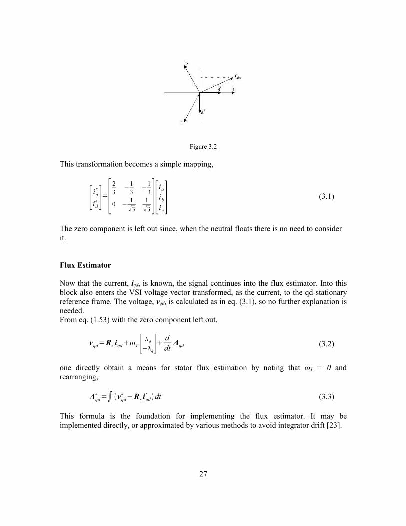
Figure 3.2

This transformation becomes a simple mapping,

[iqs

ids ]=[ 2

3−1

3−1

3

0 − 13

13 ][ia

ib

ic] (3.1)

The zero component is left out since, when the neutral floats there is no need to considerit.

Flux Estimator

Now that the current, iqd, is known, the signal continues into the flux estimator. Into thisblock also enters the VSI voltage vector transformed, as the current, to the qd-stationaryreference frame. The voltage, vqd, is calculated as in eq. (3.1), so no further explanation isneeded.From eq. (1.53) with the zero component left out,

vqd=Rs iqdωT[ d

−q] ddtΛqd (3.2)

one directly obtain a means for stator flux estimation by noting that ωT = 0 andrearranging,

Λqds =∫vqd

s −Rs iqds dt (3.3)

This formula is the foundation for implementing the flux estimator. It may beimplemented directly, or approximated by various methods to avoid integrator drift [23].

27

Sector Calculation

The control action taken by the DTC control is based on the states of the flux and torquehysteresis comparators. Flux is increased by applying a vector pointing in the flux Λs

qd-direction and torque is increased by applying a vector pointing in the rotational direction.In order to do this, the angular position of the stator flux vector must be known so that theDTC can chose between an appropriate set of vectors depending on the flux position.

Figure 3.3, DTC sectors and reference axes

Each sector spans 60º degrees; the sectors are numbered as in fig. 3.3.As seen from the picture the angle θλs can be found from

tan θ λs=−λd

s

λqs (3.4)

If λqd belongs to sector 1, switch vectors, u2, u3, u5 and u6 are used.

Figure 3.4, VSI vectors used when λqd is in sector 1

The block under Sector Calculation computes the vector norm before estimated flux, λs, ispassed on and compared with the command value, λ*

s.

28

Torque Calculation

From eq. (1.70),

T e=3 P4 λd iq−λq id (3.5)

which is true for all qd-reference frames. To calculate torque one only has to substitutethe corresponding, already, calculated fluxes and currents. Torque calculation is thus asimple operation.

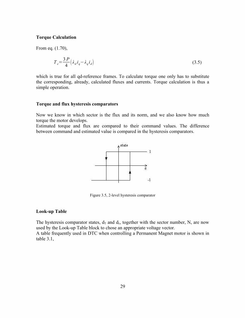
Torque and flux hysteresis comparators

Now we know in which sector is the flux and its norm, and we also know how muchtorque the motor develops.Estimated torque and flux are compared to their command values. The differencebetween command and estimated value is compared in the hysteresis comparators.

Figure 3.5, 2-level hysteresis comparator

Look-up Table

The hysteresis comparator states, dT and dλ, together with the sector number, N, are nowused by the Look-up Table block to chose an appropriate voltage vector.A table frequently used in DTC when controlling a Permanent Magnet motor is shown intable 3.1,

29

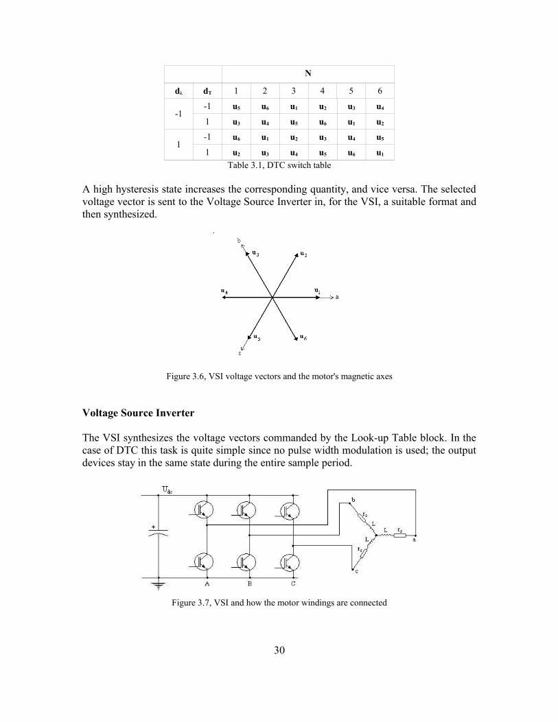
N

dλ dT 1 2 3 4 5 6

-1-1 u5 u6 u1 u2 u3 u4

1 u3 u4 u5 u6 u1 u2

1-1 u6 u1 u2 u3 u4 u5

1 u2 u3 u4 u5 u6 u1

Table 3.1, DTC switch table

A high hysteresis state increases the corresponding quantity, and vice versa. The selectedvoltage vector is sent to the Voltage Source Inverter in, for the VSI, a suitable format andthen synthesized.

Figure 3.6, VSI voltage vectors and the motor's magnetic axes

Voltage Source Inverter

The VSI synthesizes the voltage vectors commanded by the Look-up Table block. In thecase of DTC this task is quite simple since no pulse width modulation is used; the outputdevices stay in the same state during the entire sample period.

Figure 3.7, VSI and how the motor windings are connected

30

Figure 3.7 shows a simplified sketch of the VSI output stage, and how the motorwindings are connected.The output-signals from the Look-up Table block in Fig. 3.1 are named Sa, Sb and Sc.These are boolean variables indicating the switch state in the inverter output-branches.

Let Si = 1 when the high or upper switch is on and the lower is off, and Si = 0 when thelower is on and the upper off. The inverter states, (Sa Sb Sc), generating each voltagevector, then, are

u1 = (1 0 0), u2 = (1 1 0), u3 = (0 1 0), u4 = (0 1 1), u5 = (0 0 1), u6 = (1 0 1)

3.2. Torque and Flux equations

This chapter is intended to show how applied voltage vectors affect flux and torque. Theresults will lead to a better understanding of how the switch table is constructed. Alsosome problems encountered with the DTC control are illuminated. First some additionalresults to chapter 1 are presented.

In chapter 1 electromagnetic torque was given as

T e=3 P4 λd iq – λq id (3.6)

Let torque be a vector defined by the cross-product between two vectors and following aleft/right-hand rule depending on the coordinate system.As the motors neutral point is floating one does not need to care about the zero-component, hence the motor is modeled in two dimensions, q and d.Let's consider the qd coordinate system lying in the abc-plane. This plane is a crosssection of the motor.We now introduce a new coordinate, z, pointing as figure 3.8 along the rotor axis.This new coordinate system, (q,d,z), is a left hand system.

31

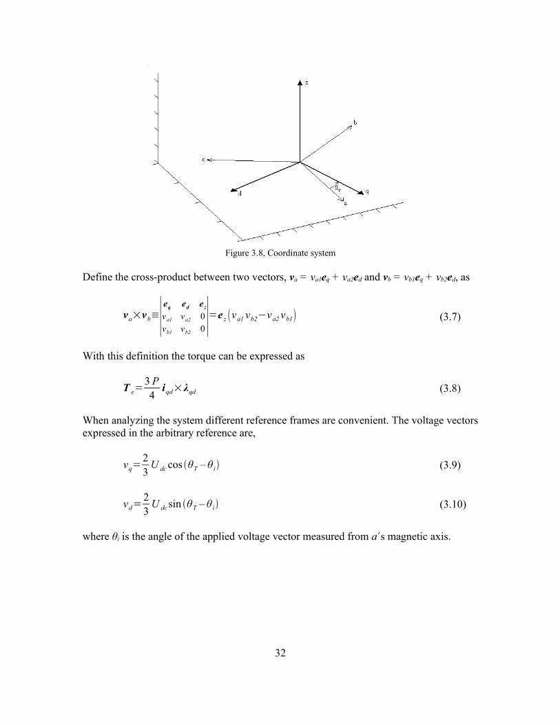
Figure 3.8, Coordinate system

Define the cross-product between two vectors, va = va1eq + va2ed and vb = vb1eq + vb2ed, as

va×vb≡∣eq ed e zva1 va2 0vb1 vb2 0∣=e z va1 vb2−va2 vb1 (3.7)

With this definition the torque can be expressed as

T e=3 P4iqd×λqd (3.8)

When analyzing the system different reference frames are convenient. The voltage vectorsexpressed in the arbitrary reference are,

vq=23

U dc cos θT – θ i (3.9)

vd=23

U dc sin θT – θ i (3.10)

where θi is the angle of the applied voltage vector measured from a´s magnetic axis.

32

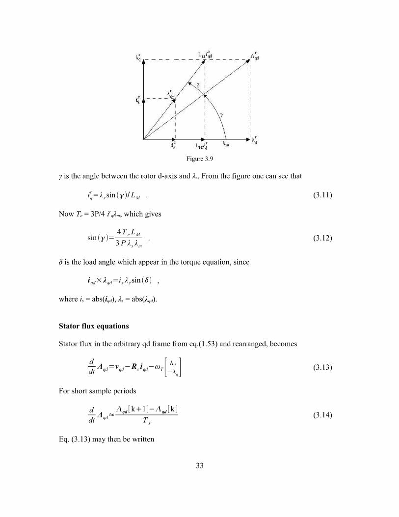
Figure 3.9

γ is the angle between the rotor d-axis and λs. From the figure one can see that

iqr=λs sin /LM . (3.11)

Now Te = 3P/4 irqλm, which gives

sin =4T e LM

3 P λs λm. (3.12)

δ is the load angle which appear in the torque equation, since

iqd×λqd=i s λs sin ,

where is = abs(iqd), λs = abs(λqd).

Stator flux equations

Stator flux in the arbitrary qd frame from eq.(1.53) and rearranged, becomes

ddtΛqd=vqd−Rs i qd−ωT[ d

−q] (3.13)

For short sample periods

ddtΛqd≈

qd [k1]−qd [k ]T s

(3.14)

Eq. (3.13) may then be written

33

λq [k1]=T s vq [k ]– r s iq [k ]– ωT λd [k ]λq [k ] (3.15)

λd [k1]=T s vd [k ]– r s id [k ]ωT λq [k ]λd [k ] (3.16)

or alternatively eq. (3.13) is rewritten,

λqt =∫vq−r s iq−ωT λd dt (3.17)

λd t =∫vd−r sidωT λqdt (3.18)

During a sufficiently short time interval, all variables on the right hand side may beapproximated constant. Thus,

λq [k ]=T s vq [k ]– r s iq[k ]– ωT λd [k ] (3.19)

λd [k ]=T s vd [k ]– r s id [k ]ωT λq [k ] (3.20)

Rotor reference

In the rotor reference the equations that describe how flux changes during the next sampleperiod becomes

λqr [k ]=T s vq

r [k ]– r s iqr [k ]– ωr λd

r [k ] (3.21)

λdr [k ]=T s vd

r [k ]– r s idr [k ]ωr λq

r [k ] (3.22)

Figure 3.10, Rotor reference flux

Here an interesting property can be seen.If torque requirement is high ir

q must be high since this is the variable causing torque in asalient free motor (see eq. 1.71), hence λr

q is high. This in turn induces a high positivevoltage in the dr-direction (along the permanent magnet). This voltage increase ir

d and

34

hence λrd. A high λr

d counteract vrq and, when velocity and/or flux are sufficiently high,

makes the resultant voltage in the qr-direction negative which lower λrq or equivalently ir

q

which produced torque.This short discussion shows that a motor has to be demagnetized when speed is high, inorder to work properly. That is, ir

d must be negative so as to counteract the permanentmagnet flux. This operational mode is often referred to as the flux weakening region.

λs – reference

Assume the qd coordinates rotate in synchronism with the stator flux, and the d-axis isaligned with the flux vector. Then,

λqλs [k ]=T s vq

λs[k ]– r s iqλs [k ]– ωr λs [k ] (3.23)

λdλs [k ]=T svd

λs[k ]– r s idλs [k ] (3.24)

Figure 3.11, λs - reference

Stator reference

In the stationary reference frame eq. (3.13) becomes

ddtΛqd

s =vqds −Rs iqd

s (3.25)

⇔Λqd

s =∫vqds −Rs iqd

s dt (3.26)

The change in flux during one switching period is obtained if the integral is evaluatedfrom t: t → t + Ts.Observe that applied voltage is constant during the switching period ⇒

35

Λqds =T s vqd

s −∫Rs iqds dt (3.27)

If the current variation is small between two consecutive samples and furthermore if rsiqd

is small compared to vqd, which is normally the case, then

Λqds =T s vqd

s −T sRs iqds (3.28)

When the resistive voltage drop is low, the last term can be left out. In this case thechange in stator flux is directly proportional to amplitude and direction of the appliedvoltage vector.

Λqds =T s vqd

s (3.29)

Here another feature of the PM motor may be noted.Since the permanent magnet always produce a flux linkage through the stator windings,flux moves even if a zero voltage vector is applied whenever the rotor evolves [16,17].This is contrary to an induction motor where stator flux is kept almost fixed in amplitudeand space when a zero voltage vector is applied.For very short time periods, though, the permanent magnet is almost fixed in space.

Torque equations

From eq. (3.8) torque can be expressed as

T e=3 P4i qd× λqd . (3.30)

Differentiate eq. (3.30),

ddt

T e=3 P4 d

dti qd×λqdiqd×

ddtλqd (3.31)

From eqs. (1.61) and (1.62) for a non-salient motor

ddtiqd

r = 1LM vqd

r −Rs iqdr – ωr[ d

r

−qr] (3.32)

If we now substitute eqs. (3.13) and (3.32) into eq.(3.31) and making use of the cross-product and torque equation (3.30), one obtains

36

ddt

T e=3 P

4 LMvq

r – ωr λdr λm –

4 r s

3 PT ee z . (3.33)

For small Ts

ddt

T e≈T e [k1]−T e [k ]

T s(3.34)

which gives

T e [k ]=3 PT s

4 LMvq

r [k ]−ωr λdr [k ] λm−

4 r s

3 PT e [k ] (3.35)

From the above expressions it can be seen how torque is affected depending on workingconditions. As can be seen, the last term, -4rs/(3P)Te, always tries to counteract the torqueand make it approach the origin.

Assume motor operation and positive rotational direction. Then the average vrq is

positive, speed induced voltage, -ωr λrd, negative, and an asymmetry becomes clear.

If torque is too low and need to be increased a positive vrq is chosen, but because of -ωrλr

d

is suppressed and increasing torque becomes more difficult at high velocities. On theother hand, if torque is too high, a negative vr

q is chosen but is now boosted which maketorque decreases more at high velocities.

It is always reasonable to assume λrd > 0. If λr

d should be negative the demagnetizing fluxmust be greater than the flux produced by the permanent magnet which may demagnetizethe magnet permanently.

3.3. System analysis

Now when all results needed for analysis purposes are obtained we can start looking atthe results.

To see how the voltage selection criterion is made it is good to know how the voltagevectors influence flux and torque over a sector.From the orientation of the λs-reference one can see that vd

λs is the component controllingthe flux, because vd

λs is aligned with the flux vector. It seems reasonable to assume thenthat vq

λs is responsible for the torque control.

37

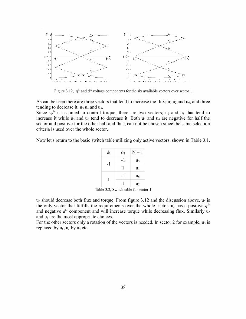
Figure 3.12, qλs and dλs voltage components for the six available vectors over sector 1

As can be seen there are three vectors that tend to increase the flux; u1 u2 and u6, and threetending to decrease it; u3 u4 and u5.Since vq

λs is assumed to control torque, there are two vectors; u2 and u3 that tend toincrease it while u5 and u6 tend to decrease it. Both u1 and u4 are negative for half thesector and positive for the other half and thus, can not be chosen since the same selectioncriteria is used over the whole sector.

Now let's return to the basic switch table utilizing only active vectors, shown in Table 3.1.

dλ dT N = 1

-1-1 u5

1 u3

1-1 u6

1 u2

Table 3.2, Switch table for sector 1

u5 should decrease both flux and torque. From figure 3.12 and the discussion above, u5 isthe only vector that fulfills the requirements over the whole sector. u3 has a positive qλs

and negative dλs component and will increase torque while decreasing flux. Similarly u2

and u6 are the most appropriate choices.For the other sectors only a rotation of the vectors is needed. In sector 2 for example, u5 isreplaced by u6, u3 by u4 etc.

38

Figure 3.13, How DTC chose switch vectors depending on torque and flux

Figure 3.13 shows the DTC voltage vector selection in sector 1. The dashed lines arecommand values and solid lines hysteresis thresholds.

Eq. (3.35),

T e [k ]=3 PT s

4 LMvq

r [k ]−ωr λdr [k ] λm−

4 r s

3 PT e [k ] . (3.36)

Divide this equation into two contributions,

T e=T 2T 1 . (3.37)

The first contribution

T 1=– T sr s

LMT e (3.38)

always tries to lower the torque value. The second contribution,

T 2=3 PT s

4 LMvq

r−ωr λdr λm , (3.39)

is the component controlled by the applied voltage vector. The voltage vector controllingtorque and the flux component giving rise to the emf are both expressed in the rotorreference. From figure 3.9 and 3.11

vqr=vq

λs cos (3.40)

39

andλd

r=λs cos . (3.41)

Thus, when ΔT2 is expressed in the λs-reference it becomes

T 2=3 PT s

4 LMvq

λs−ωr λs λm cos . (3.42)

The relation between applied vector and emf is maintained. The difference is that when γgrows the effect of vq

λs on ΔT2 is weaker.In the extreme case, when γ = +/- 90º, vq

λs no longer affects torque but is insteadcontrolled by vd

λs. This happens if the demagnetizing flux, LMird, exactly cancels the

magnet flux. Hence, if γ becomes too big, decoupled flux and torque control is no longerpossible, and the control strategy used in DTC does not work.

But because γ is normally quite small this is seldom a problem. For example the motorused in the experiments has a nominal current of 5A, a q-axis inductance of 0.043H and aPM flux of 0.49Wb. That is, when the nominal current is directed along the qr-axis, toobtain maximum torque per ampere ratio, cos(γ) ≈ 0.9, which is close to one.

Only when the motor is hardly demagnetized, as may be the case in the flux weakeningregion, the difference becomes important.

Figure 3.14, How torque producing component vrq depends on flux angle and γ

The above figure shows how the torque producing component, vrq, depends on the flux

and γ when u2 is applied and λs is in sector 1.

Depending on the operating conditions a given voltage vector may affect torque quitedifferently. When the rotor evolves an emf is induced in the stator windings. This voltage,ωrλd, has the same direction as vq in motor operation.

40

Figure 3.15, Induced emf change the effect of a voltagevector on torque

This emf makes an increase of torque value more difficult when speed is high while adecrease is more significant. Another effect is that if speed is low and torque is close tothe desired value a zero vector may be applied. A zero vector “locks” the stator current atits actual value and position and hence, if rotor movement may be neglected (which is thecase for short Ts and low speed), maintains torque at the same value.For high speeds a zero vector will decrease torque because of ωrλd, as seen in the figure.This problem is dealt with in the DSVM scheme, where more voltage vectors areavailable.

3.4. Some problems with the basic DTC system

Torque ripple

A mayor disadvantage with the DTC control is its high torque ripple. In someapplications this may not be a problem, rotor and load inertia filters the ripple, while insome applications low torque ripple is essential.A Field Oriented Controller produce less ripple but has the drawback of being morecomplex and less robust than a DTC controller.

Drift in Flux Estimator

Direct Torque Control is very robust because it only uses one system parameter, statorwinding resistance. This parameter, however, affects the stator flux estimation which isthe heart of a DTC.A deviance in stator resistance cause an under or over estimation of stator flux, if theestimator is implemented as an integrator, even the smallest discrepancy will eventuallymake the integrator drift away.Since a DTC control system normally is implemented in discrete time and nomeasurement can ever be perfect, a pure integrator is prone to drift.

41

Stator resistance has a high influence on flux estimation, especially at low speed whereresistive voltage drop is comparable with the speed voltage.During operation stator resistance will change due to temperature changes caused bycopper losses in stator windings, heating in nonlinear magnetic materials, etc. The statorresistance may change by about 1.5 – 1.7 times of its nominal value [23].When the difference between actual resistance and the value used in flux estimationbecomes sufficiently large, the control system may become unstable.A solution to minimize this problem is to use an online resistance estimator.If actual resistance is larger than that used in the flux estimation, an overestimation offlux will result. The flux then gives an overestimation of calculated torque.If the resistance were not different, current had to differ from its measured value. Thisdifference in measured and a hypothetical current can drive a PI-estimator that tracks theresistance. The integral part force estimated resistance to converge to its real value untilthere is no difference between the hypothetical and measured current.

The problem with integrator drift may be solved by using n cascaded low-pass filters.If n 1:st order filters are connected in series the total phase shift and gain become

T=n arctan (3.43)

K T=12−n2 . (3.44)

For the cascaded filters to work as an integrator their total phase shift should be 90º andcompensation gain must be used so that the overall gain is 1/ω. From these conditions onecalculates the time constant and compensating gain,

= 1

tan 2 n

(3.45)

G= 112

n2 . (3.46)

The LPFs cannot operate as an integrator for zero frequency because time constant andgain becomes infinite. The method has the drawback of requiring more computations butdoes not drift and therefore significantly improves drive performance.

Summary

Chapter 3 begun with an explanation of the DTC scheme's different blocks. Section 3.2express the flux vector in different reference frames and derive an equation for the torque.From these expressions one can see how the DTC voltage vector selection strategy ismade.

42

Different working conditions influence how a given voltage vector affect flux and torque.Torque ripple will be symmetrical around its reference value at low speed while at higherspeeds the emf voltage tries to decrease torque and eventually makes it impossible toincrease. For high velocities the rotor flux must be weakened in order for the machine tobe able to produce torque.An advantage of DTC is the possibility of not requiring a position decoder duringoperation. The flux vector estimator, which is the heart of a DTC, only needs to know thestator winding resistance and initial rotor position. If care is not taken when operating aDTC system sensor-less the drive system will be prone to instability. On-line estimationof stator resistance and the use of cascaded low-pass filters to perform the requiredintegration are two viable solutions to minimize the problems and enhance driveperformance.

43

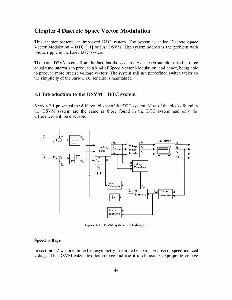
Chapter 4 Discrete Space Vector Modulation

This chapter presents an improved DTC system. The system is called Discrete SpaceVector Modulation – DTC [11] or just DSVM. The system addresses the problem withtorque ripple in the basic DTC system.

The name DSVM stems from the fact that the system divides each sample period in threeequal time intervals to produce a kind of Space Vector Modulation, and hence, being ableto produce more precise voltage vectors. The system still use predefined switch tables sothe simplicity of the basic DTC scheme is maintained.

4.1 Introduction to the DSVM – DTC system

Section 3.1 presented the different blocks of the DTC system. Most of the blocks found inthe DSVM system are the same as those found in the DTC system and only thedifferences will be discussed.

Figure 4.1, DSVM system block diagram

Speed voltage

In section 3.2 was mentioned an asymmetry in torque behavior because of speed inducedvoltage. The DSVM calculates this voltage and use it to choose an appropriate voltage

44

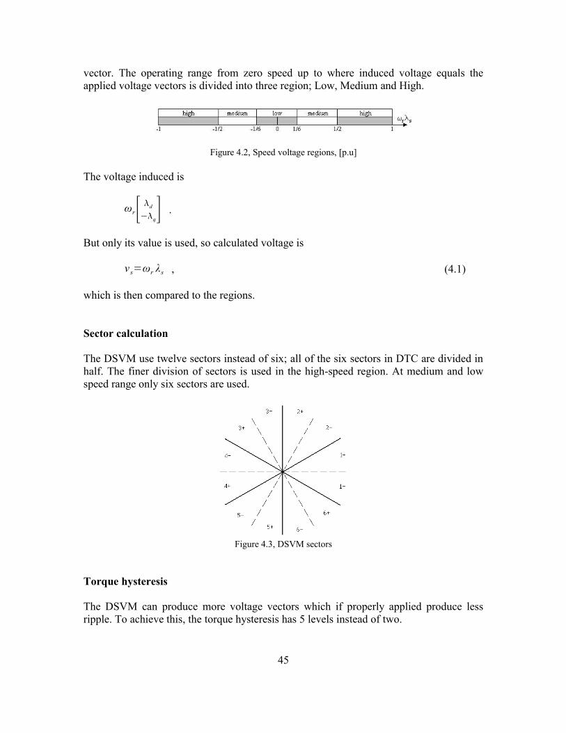
vector. The operating range from zero speed up to where induced voltage equals theapplied voltage vectors is divided into three region; Low, Medium and High.

Figure 4.2, Speed voltage regions, [p.u]

The voltage induced is

ωr[ d

−q] .

But only its value is used, so calculated voltage is

v s=ωr λs , (4.1)

which is then compared to the regions.

Sector calculation

The DSVM use twelve sectors instead of six; all of the six sectors in DTC are divided inhalf. The finer division of sectors is used in the high-speed region. At medium and lowspeed range only six sectors are used.

Figure 4.3, DSVM sectors

Torque hysteresis

The DSVM can produce more voltage vectors which if properly applied produce lessripple. To achieve this, the torque hysteresis has 5 levels instead of two.

45

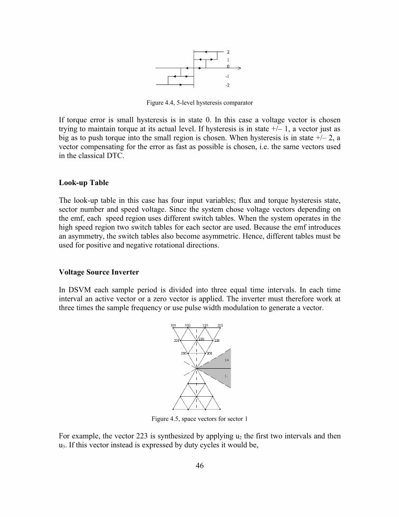
Figure 4.4, 5-level hysteresis comparator

If torque error is small hysteresis is in state 0. In this case a voltage vector is chosentrying to maintain torque at its actual level. If hysteresis is in state +/– 1, a vector just asbig as to push torque into the small region is chosen. When hysteresis is in state +/– 2, avector compensating for the error as fast as possible is chosen, i.e. the same vectors usedin the classical DTC.

Look-up Table

The look-up table in this case has four input variables; flux and torque hysteresis state,sector number and speed voltage. Since the system chose voltage vectors depending onthe emf, each speed region uses different switch tables. When the system operates in thehigh speed region two switch tables for each sector are used. Because the emf introducesan asymmetry, the switch tables also become asymmetric. Hence, different tables must beused for positive and negative rotational directions.

Voltage Source Inverter

In DSVM each sample period is divided into three equal time intervals. In each timeinterval an active vector or a zero vector is applied. The inverter must therefore work atthree times the sample frequency or use pulse width modulation to generate a vector.

Figure 4.5, space vectors for sector 1

For example, the vector 223 is synthesized by applying u2 the first two intervals and thenu3. If this vector instead is expressed by duty cycles it would be,

46

vector

223

duty cycleA

0.67

B

1

C

0

This is how the inverter operated during the experiments.

4.2 Space vector selection

In chapter 3 the problems with torque ripple and the asymmetric torque behavior at highvelocities were discussed. In this section will be discussed how the higher number ofavailable voltage vectors can be utilized to reduce these problems.

When speed increase the induced emf, vs, also increase. The voltage vector vs leads λs by90º and lies along the qλs-axis. The resultant vector that affects torque is the vq

λs

component of the applied VSI vector minus vs. Therefore, the voltage selection criteriashould use vs as a reference; if vq

λs ≈ vs torque is kept at the same level, vqλs > vs increase

torque and vqλs < vs decrease it.

Low-speed region

When vs is in the low-speed region, vs is close to zero. The switch vectors are selectedsymmetrically around zero, which also connects the gap between positive and negativespeed switch tables.If estimated torque is close to its reference value and torque hysteresis is in state zero, thezero vector is chosen. If torque hysteresis is in state +1 or -1, a moderate increase ordecrease, respectively, is wanted. Selection is made between u200, u300, u500 and u600. u200

and u600 is the choice if flux is to be increased while u300 and u500 decrease flux. When thedifference is big between estimated and reference torque, i.e. dT = +/-2, DSVM choosesswitch vectors as the DTC. Here vectors u222, u333, u555, and u666 are selected in order tocompensate for the deviation as fast as possible.

dT

-2 -1 0 1 2

dλ-1 555 500 000 300 3331 666 600 000 200 222

Table 4.1, Switch table for positive low-speed region, sector 1

47

Medium-speed region

In the medium-speed region, vN/6 < |vs| < vN/2, the emf voltage starts to introduce anasymmetry of the switch vectors on torque behavior. For positive vs and dT = 0, DSVMchose between u200 and u300, since these vectors makes vq

λs approximately equal to vs andhence maintains torque at its actual level. u200 is the choice if flux should be increased andu300 if decreased. For dT = -1 a moderate torque decrease is wanted. Now the closestvector decreasing torque is u000, and since this is the only vector at this level it is chosenweather flux is lower or higher than its reference value. For dT = +1, u220 is selected whenflux should be raised and u330 when lowered. As in the low speed region, DSVM operatesas the DTC when dT = +/- 2.

dT

-2 -1 0 1 2

dλ-1 555 000 300 330 3331 666 000 200 220 222

Table 4.2, Switch table for positive medium-speed region, sector 1

High-speed region

In the high-speed region, |vs| > vN/2. To make use of all vectors available each sector isdivided in half.Assume λs is in sector 1- . Then if torque is to be kept at the same level, vectors u220 andu230 are selected depending on the flux comparator. For dT = -1, the nearest lower vq

λs

voltage is obtained by choosing u200 or u300. For dT = +1, u222 and u223 will increase fluxwhile u332 and u333 will decrease flux. To make full use of all switch vectors and to keepflux ripple at a low level, u222 and u332 are chosen for λs lying in sector 1-. When λs is insector 1+, u230 and u330 is the choice for dT = 0, while u223 and u333 are chosen for dT = +1.In the high speed region as in the low and medium, the maximal vectors available areselected for dT = +/- 2.

dT

-2 -1 0 1 2

dλ-1 555 300 230 332 3331 666 200 220 222 222

Table 4.3, Switch table for positive high-speed region, sector 1-

48

dT

-2 -1 0 1 2

dλ-1 555 300 330 333 3331 666 200 230 223 222

Table 4.4, Switch table for positive high-speed region, sector 1+

Summary

The DSVM system divides each sample period in three equal time intervals to produce akind of Space Vector Modulation. The system calculates the emf voltage which is used inthe voltage selection procedure. If torque is close to its reference value a voltage spacevector lying approximately on the emf voltage line is chosen. The space vectors next tothe emf voltage levels are used for small torque corrections. For large torque errorsDSVM operates as the basic DTC system. Torque ripple is reduced to approximately onethird with respect to the basic DTC control. The system maintains a good dynamic torqueresponse, which is characteristic for DTC, while still having a relatively low complexity;DSVM select a voltage space vector from predefined switch tables.A comparison with the basic DTC can be seen in the next chapter where results fromsimulations and experiment are presented.

49

Chapter 5 Simulation and experimental results

In chapter 3 and 4 the DTC and DSVM systems were explained in detail. Here simulationand experimental results of the two systems are presented.

Simulation models are programmed in Matlab/Simulink, operating at a sample frequencyof 10 kHz. Experimental arrangement consist of a dSPACE DS1103 board, connected toa Danfoss VLT5003 inverter. The PM motor is a Siemens 1FT6062-6AC7. To control thebreaking torque another Siemens 1FT6084 motor is used connected to a SiemensSIMOVERT MC inverter which is controlled by the dSPACE environment.The experiments were executed with a sample frequency of 20 kHz. Increased ripple,measure noise and conservative protections would otherwise obscure the interesting partsof the experiments.

Simulation results

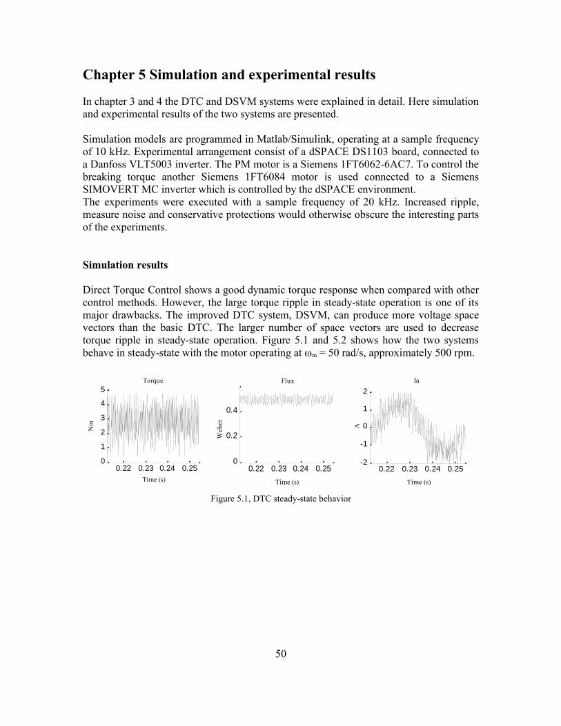
Direct Torque Control shows a good dynamic torque response when compared with othercontrol methods. However, the large torque ripple in steady-state operation is one of itsmajor drawbacks. The improved DTC system, DSVM, can produce more voltage spacevectors than the basic DTC. The larger number of space vectors are used to decreasetorque ripple in steady-state operation. Figure 5.1 and 5.2 shows how the two systemsbehave in steady-state with the motor operating at ωm = 50 rad/s, approximately 500 rpm.

Figure 5.1, DTC steady-state behavior

50

0.22 0.23 0.24 0.250

1

2

3

4

5Torque

Time (s)

Nm

0.22 0.23 0.24 0.25-2

-1

0

1

2

Ia

Time (s)

A

0.22 0.23 0.24 0.250

0.2

0.4

Flux

Time (s)

Web

er

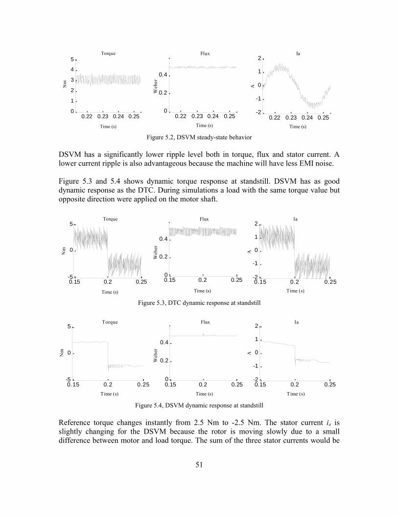
Figure 5.2, DSVM steady-state behavior

DSVM has a significantly lower ripple level both in torque, flux and stator current. Alower current ripple is also advantageous because the machine will have less EMI noise.

Figure 5.3 and 5.4 shows dynamic torque response at standstill. DSVM has as gooddynamic response as the DTC. During simulations a load with the same torque value butopposite direction were applied on the motor shaft.

Figure 5.3, DTC dynamic response at standstill

Figure 5.4, DSVM dynamic response at standstill

Reference torque changes instantly from 2.5 Nm to -2.5 Nm. The stator current ia isslightly changing for the DSVM because the rotor is moving slowly due to a smalldifference between motor and load torque. The sum of the three stator currents would be

51

0.22 0.23 0.24 0.250

1

2

3

4

5Torque

Time (s)

Nm

0.22 0.23 0.24 0.250

0.2

0.4

Flux

Time (s)

Web

er

0.22 0.23 0.24 0.25-2

-1

0

1

2Ia

Time (s)

A

0.15 0.2 0.25-5

0

5Torque

Time (s)

Nm

0.15 0.2 0.250

0.2

0.4

Flux

Time (s)

Web

er

0.15 0.2 0.25-2

-1

0

1

2Ia

Time (s)

A

0.15 0.2 0.25-5

0

5Torque

Time (s)

Nm

0.15 0.2 0.250

0.2

0.4

Flux

Time (s)

Web

er

0.15 0.2 0.25-2

-1

0

1

2Ia

Time (s)

A

a slowly moving vector with constant amplitude.

Experimental results

Both systems have been tested experimentally in order to verify the improvements of theproposed method. Steady-state and dynamic response results were obtained under thesame conditions as in simulations with the exception of a higher sample frequency.

Figure 5.5 and 5.6 shows steady-state behavior for the DTC and DSVM, respectively.The motor operates at ωm = 50 rad/s, approximately 500 rpm. The relative decrease inripple levels in the DSVM is similar to simulations.

Figure 5.5, DTC steady-state behavior

Figure 5.6, DSVM steady-state behavior

Dynamic response measurements were taken with the rotor at approx. standstill, wherethe load was a motor giving the same torque but in the opposite direction. Torque isgreatly reduced with the DSVM scheme. Ripple reduction complies well with eq. (3.35)predicting a torque ripple reduction to 1/3 compared with the basic DTC scheme, sinceeach sample interval is divided into three equal parts.

52

0 0.01 0.02 0.03 0.04-3

-2

-1

0

1

2

3

A

Ia

Time (s)

0 0.01 0.02 0.03 0.040

2

4

6

Nm

Torque

Time (s)

0 0.01 0.02 0.03 0.040

0.2

0.4

Wb

Flux

Time (s)

Web

er

0 0.02 0.040

2

4

6Torque

Time (s)

Nm

0 0.02 0.040

0.2

0.4

Flux

Time (s)

Web

er

0 0.02 0.04

-2

0

2

Ia

Time (s)

A

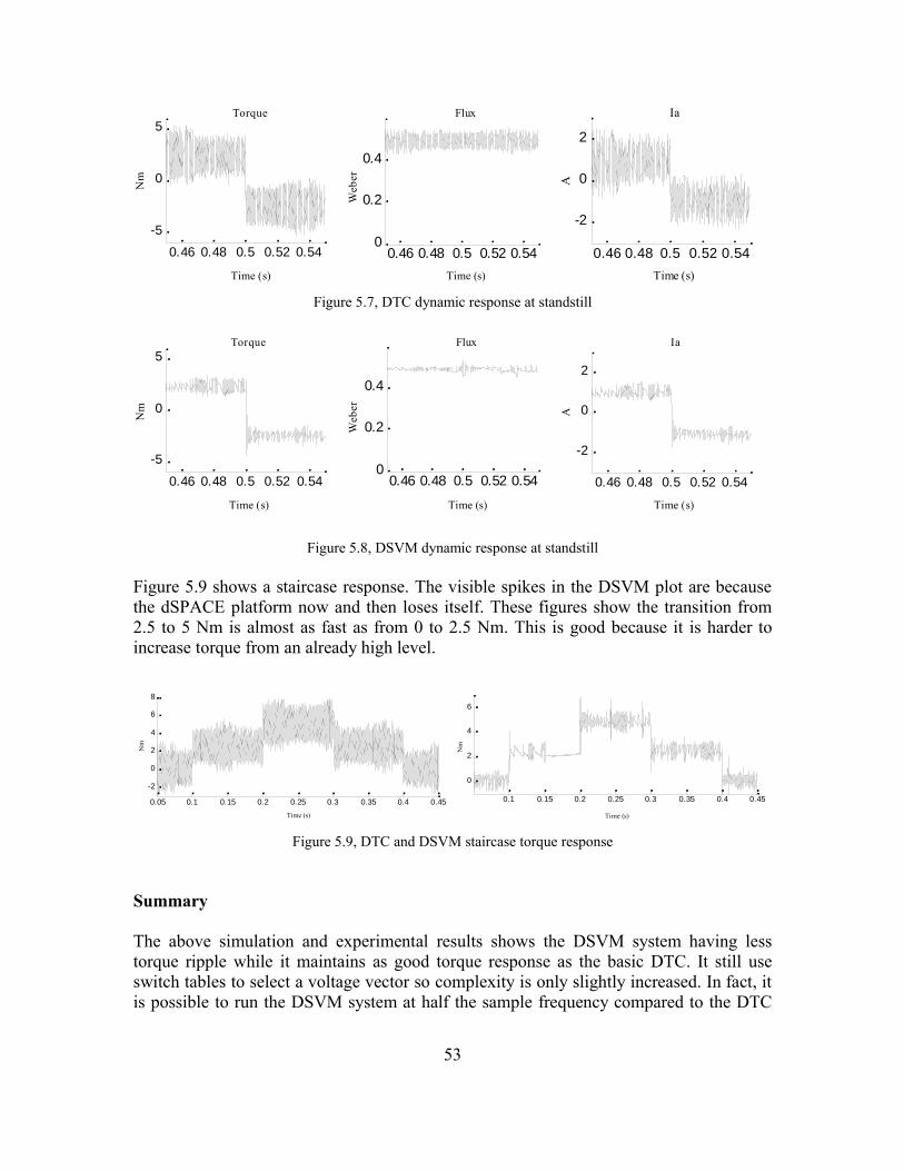
Figure 5.7, DTC dynamic response at standstill

Figure 5.8, DSVM dynamic response at standstill

Figure 5.9 shows a staircase response. The visible spikes in the DSVM plot are becausethe dSPACE platform now and then loses itself. These figures show the transition from2.5 to 5 Nm is almost as fast as from 0 to 2.5 Nm. This is good because it is harder toincrease torque from an already high level.

Figure 5.9, DTC and DSVM staircase torque response

Summary

The above simulation and experimental results shows the DSVM system having lesstorque ripple while it maintains as good torque response as the basic DTC. It still useswitch tables to select a voltage vector so complexity is only slightly increased. In fact, itis possible to run the DSVM system at half the sample frequency compared to the DTC

53

0.46 0.48 0.5 0.52 0.54

-5

0

5Torque

Time (s)

Nm

0.46 0.48 0.5 0.52 0.540

0.2

0.4

Flux

Time (s)

Web

er

0.46 0.48 0.5 0.52 0.54

-2

0

2

Ia

Time (s)

A

0.46 0.48 0.5 0.52 0.54

-5

0

5Torque

Time (s)

Nm

0.46 0.48 0.5 0.52 0.540

0.2

0.4

Flux

Time (s)

Web

er

0.46 0.48 0.5 0.52 0.54

-2

0

2

Ia

Time (s)

A

0.05 0.1 0.15 0.2 0.25 0.3 0.35 0.4 0.45

-2

0

2

4

6

8

Nm Nm

Time (s)

0.1 0.15 0.2 0.25 0.3 0.35 0.4 0.45

0

2

4

6

Nm

Nm

Time (s)

and still obtain equal or lower ripple levels. DSVM would in this case require less of theprocessor.

54

Chapter 6 Conclusion

This work has dealt with the Direct Torque Control and one of its improved variantsproposed in the research literature. DTC was introduced in the 1980´s by I. Takahashi, T.Noguchi and M. Depenbrock (DSC) and was a novel control technique for InductionMotor vector control. Vector control was introduced in 1972 by F. Blaschke which wasthe technique since known as Field Oriented Control.In vector control both amplitude and position of the field flux is known, so the controllercan control the armature flux amplitude and angle relative the field flux. In a DC motorthe field flux, which in this case is the stator flux, and the armature flux (rotor) are heldorthogonal mechanically by the commutator. When the fields are orthogonal, armatureflux does not affect the field flux and the motor torque responds immediately to a changein armature flux or equivalently, armature current. In an AC motor the field flux (whichnow is in the rotor) rotates, but in a FOC the controller rotates the armature (stator) fluxso that armature and field flux are kept orthogonal, and hence, the motor-controllersystem behaves as a DC motor system.The principle behind Direct Torque Control is quite the same, with the difference thecontrol action is tabulated instead of being calculated online. DTC being more crude hasthe advantage of not having to compute applied current/voltage vectors, whichsignificantly lowers the computational burden. This allows for a pretty simple, and cheap,processor to perform the task. Another feature of not computing the CSI or VSI vectorsonline is that fewer motor parameters are involved in the control, which improvesrobustness.The decreased performance of DTC drives in terms of torque, flux and current ripple,with respect to FOC, is partly compensated for by its simplicity since this allows forhigher sample frequencies. The problem is that the inverter sets an upper limit for itsswitching frequency.Since the introduction of DTC a lot of research has been done to improve performance ofDTC drives while maintaining the good properties, such as

• low complexity• good dynamic response• high robustness.

In this work one of the many improved DTC systems proposed is presented. Simulationand experimental results confirms its validity.The new DTC system called Discrete Space Vector Modulation – DTC or just DSVM,use a kind of space vector modulation to produce more voltage vectors than are availablewith the classical DTC. DSVM use different look-up tables depending on the value of theemf voltage induced in the stator windings.Both the classical and improved DTC systems are simulated using Simulink and then ranon a dSPACE platform to evaluate real life behavior from the experiments. The systemsshow a higher ripple level for torque, flux and stator currents in the experiments than inthe simulations. Though, the relative decrease in ripple levels of the DSVM system

55

compared to the DTC system are equal both in experiments and simulations.

Figure 6.1, Above simulation results; left DTC, right DSVM.Below experimental results; left DTC, right DSVM.

The DSVM is a compromise between performance and low complexity because the useof look-up tables. While a large number of voltage vectors would improve performance interms of low ripple, they would require large and complex look-up tables. The benefits ofthe proposed method is that while complexity is still low, ripple levels are decreased andthe good dynamic response is maintained, which the experimental results in figure 6.2shows.

Figure 6.2, Dynamic response DTC and DSVM

There are other methods performing better than the one presented, but at the expense ofhigher complexity and computational burden.

56

0.498 0.499 0.5 0.501 0.502 0.503-5

-4

-3

-2

-1

0

1

2

3

4

5

Nm

Time (s)

DTC

0.498 0.499 0.5 0.501 0.502 0.503-5

-4

-3

-2

-1

0

1

2

3

4

5

Nm

Time (s)

DSVM

0.22 0.23 0.24 0.250

1

2

3

4

5Torque

Time (s)

Nm

0.22 0.23 0.24 0.250

1

2

3

4

5Torque

Time (s)

Nm

0 0.01 0.02 0.03 0.040

2

4

6

Nm

Torque

Time (s)

0 0.02 0.040

2

4

6Torque

Time (s)

Nm

With the introduction of Field Oriented Control, AC motors have in many applicationsreplaced DC motors where good torque control and fast dynamic response is required.The AC motor being more reliable, requiring less maintenance and being the preferredchoice in hazardous environments, e.g. if explosive gas is present, where sparks from thecommutator in a DC motor is a problem.With the commercialization of DTC, the first commercial products introduced by ABB,the technique is now being employed where before FOC drives were used.

57

References

1. Modern Power Electronics and AC DrivesBimal K.Bose2002 Prentice Hall, ISBN 0-13-016743-6

2. Dynamic simulation of Electric Machinery using Matlab/SimulinkChee-Mun Ong1998 Prentice Hall, ISBN 0-13-723785-5

3. Vector Control and Dynamics of AC DrivesD.W. Novotny, T.A. Lipo1996 Oxford University Press, ISBN 0-19-856439-2

4. Analysis of Electric Machinery and Drive Systems, Second EditionPaul C. Krause, Oleg Wasynczuk, Scott D. Sudhoff2002 IEEE Press, Wiley Interscience, ISBN 0-471-14326-X

5. Electric Machinery, fourth editionA.E. Fitzgerald, Charles Kingsley Jr., Stephen D. Umans1983 McGraw-Hill, ISBN 0-07-021145-0

6. Advanced Control System DesignBernard Friedland1996 Prentice Hall, ISBN 0-13-010653-4

7. Feedback Control of Dynamic Systems, third editionGene F. Franklin, J. David Powell, Abbas Emami-Naeini1994 Addison-Wesley, ISBN 0-201-52747-2

8. Electromechanical Systems, Electric Machines and Applied MechatronicsSergey E. LyshevskiCRC Press 2000, ISBN 0-8493-2275-8

9. Field and Wave Electromagnetics, Second EditionDavid K. Cheng1989 Addison – Wesley, ISBN 0-201-52820-7

10. Elementary Linear Algebra, 7th EditionHoward Anton, Chris Rorres1994 Wiley, ISBN 0-471-58741-9

11. Improvement of Direct Torque Control by Using a Discrete SVM TechniqueDomenico Casadei, Giovanni Serra, Angelo TaniIEEE 1998

12. Torque dynamic behavior of Induction machine DTC in 4 quadrant operationI. El Hassan, X. Roboam, B. de Fornel, E.V. WesterholtIEEE 1997

58

13. Analytical Formulation of the Direct Control of Induction Motor DrivesM. Bertoluzzo, G. Buja, R. Menis1999 IEEE

14. Direct Torque Control of Permanent Magnet Synchronous Motor (PMSM) Using Space Vector Modulation (DTC-SVM) – Simulation and Experimental ResultsDariusz Swierczynski, Mariam P. Kazmierkowski2002 IEEE

15. A New Direct Torque Control Strategy for Flux and Torque Ripple Reduction for Induction Motors Drive – A Matlab/Simulink ModelLixin Tang, M.F. Rahman2001 IEEE

16. A Direct Torque Controller for Permanent Magnet Synchronous motor drives.Zheng, M.F. Rhaman, W.Y. Hu, K.W. Lim.IEEE transactions on energy conversion, Vol. 14, No. 3, September 1999.

17. Study on the Direct Torque Control of Permanent Magnet Synchronous Motor Drives.Sun Dan, Fang Weizhong, He Yikang.Electrical Machines and Systems, IEEE 2001

18. Implementation Strategies for Concurrent Flux Weakening and Torque Control of the PM synchronous Motor.Ramin Monajemy, Ramu Krishnan.IEEE, Industry Applications Conference, 1995.

19. FOC and DTC: two viable schemes for induction motors torque control.Domenico Casadei, Fransesco Profumo, Giovanni Serra, Angelo Tani.IEEE Transactions on Power Electronics, 2001.

20. Direct torque control of induction motors: stability analysis and performance improvement.Romeo Ortega, Nikita Barabanov, Gerardo Escobar Valderrama.IEEE Transactions on Automatic Control, Vol. 46, No. 8, 2001.

21. Direct stator flux linkage control technique for a permanent magnet synchronous machine.A.M. Llor, J.M. Rétif, X. Lin-Shi, S. ArnalteIEEE 2003

22. Direct Torque Control of PWM Inverter-Fed AC Motors – A SurveyGiuseppe S. Buja, Marian P. KazmierkowskiIEEE Trans. On Industrial Electronics, Vol. 51, No. 4, August 2004

23. Problems Associated With the Direct Torque Control of an Interior Permanent-Magnet Synchronous Motor Drive and Their RemediesMuhammed Fazlur Rahman, Enamul Haque, Lixin Tang, Limin ZhongIEEE Trans. On Industrial Electronics, Vol. 51, No. 4, August 2004

59

24. A Space Vector Modulation Direct Torque Control for Permanent Magnet Synchronous Motor Drive SystemsD. Sun, J.G. Zhu, Y.K. HePower Electronics and Drive Systems, IEEE 2003

25. Study of Direct Torque Control (DTC) System of Permanent Magnet Synchronous Motor Based on DSPDai Wenjin, Li HuilingElectrical Machines and Systems, IEEE 2001

60

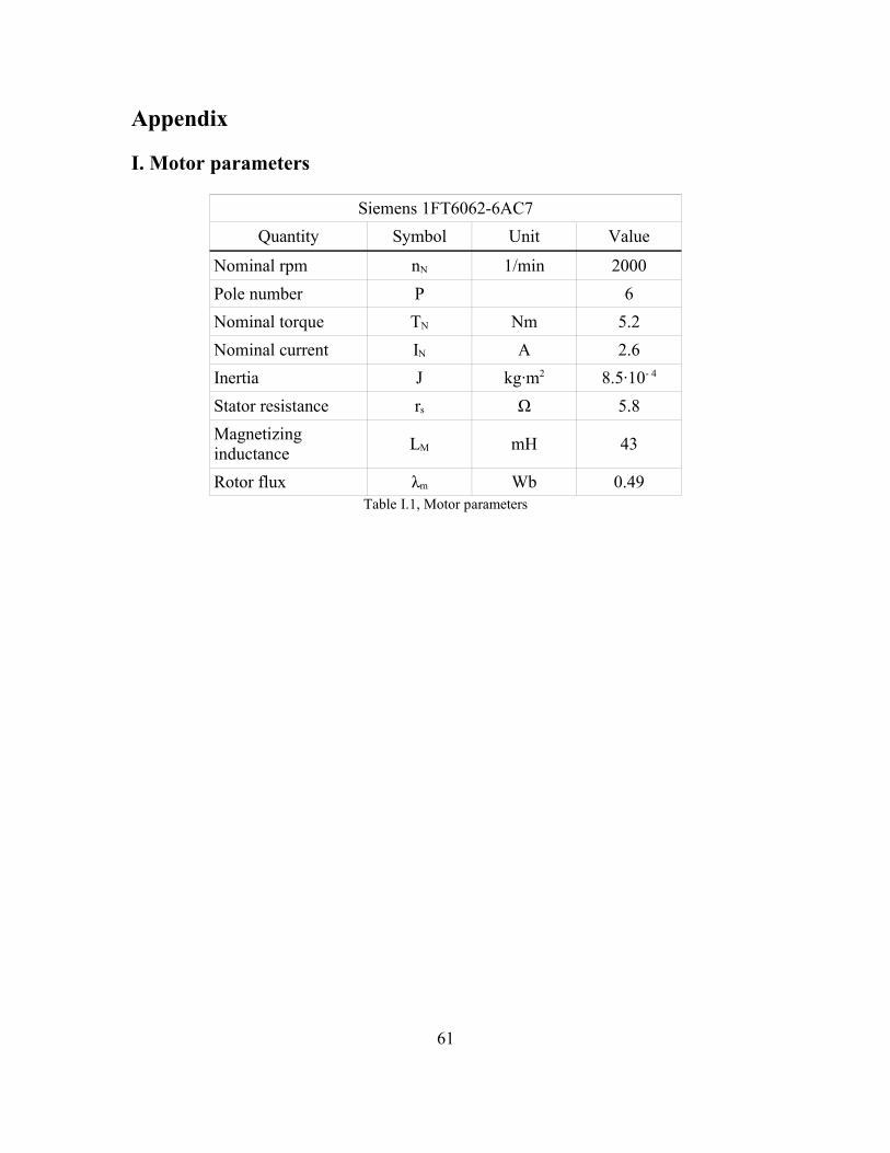
Appendix

I. Motor parameters

Siemens 1FT6062-6AC7Quantity Symbol Unit Value

Nominal rpm nN 1/min 2000Pole number P 6Nominal torque TN Nm 5.2Nominal current IN A 2.6Inertia J kg·m2 8.5·10- 4

Stator resistance rs Ω 5.8Magnetizinginductance LM mH 43

Rotor flux λm Wb 0.49Table I.1, Motor parameters

61