Embed Size (px)
Citation preview
ABSTRACT
Title of dissertation: IMPROVING THE USABILITY OF STATICANALYSIS TOOLS USING MACHINELEARNING
Ugur KocDoctor of Philosophy, 2019
Dissertation directed by: Professor Dr. Adam A. PorterDepartment of Computer ScienceProfessor Dr. Jeffrey S. FosterDepartment of Computer Science
Static analysis can be useful for developers to detect critical security flaws and
bugs in software. However, due to challenges such as scalability and undecidabil-
ity, static analysis tools often have performance and precision issues that reduce
their usability and thus limit their wide adoption. In this dissertation, we present
machine learning-based approaches to improve the adoption of static analysis tools
by addressing two usability challenges: false positive error reports and proper tool
configuration.
First, false positives are one of the main reasons developers give for not using
static analysis tools. To address this issue, we developed a novel machine learning
approach for learning directly from program code to classify the analysis results as
true or false positives. The approach has two steps: (1) data preparation that trans-
forms source code into certain input formats for processing by sophisticated machine
learning techniques; and (2) using the sophisticated machine learning techniques to

discover code structures that cause false positive error reports and to learn false
positive classification models. To evaluate the effectiveness and efficiency of this
approach, we conducted a systematic, comparative empirical study of four families
of machine learning algorithms, namely hand-engineered features, bag of words, re-
current neural networks, and graph neural networks, for classifying false positives.
In this study, we considered two application scenarios using multiple ground-truth
program sets. Overall, the results suggest that recurrent neural networks outper-
formed the other algorithms, although interesting tradeoffs are present among all
techniques. Our observations also provide insight into the future research needed to
speed the adoption of machine learning approaches in practice.
Second, many static program verification tools come with configuration op-
tions that present tradeoffs between performance, precision, and soundness to allow
users to customize the tools for their needs. However, understanding the impact of
these options and correctly tuning the configurations is a challenging task, requiring
domain expertise and extensive experimentation. To address this issue, we devel-
oped an automatic approach, auto-tune, to configure verification tools for given
target programs. The key idea of auto-tune is to leverage a meta-heuristic search
algorithm to probabilistically scan the configuration space using machine learning
models both as a fitness function and as an incorrect result filter. auto-tune is
tool- and language-agnostic, making it applicable to any off-the-shelf configurable
verification tool. To evaluate the effectiveness and efficiency of auto-tune, we ap-
plied it to four popular program verification tools for C and Java and conducted
experiments under two use-case scenarios. Overall, the results suggest that running

verification tools using auto-tune produces results that are comparable to config-
urations manually-tuned by experts, and in some cases improve upon them with
reasonable precision.

IMPROVING THE USABILITY OF STATIC ANALYSIS TOOLSUSING MACHINE LEARNING
by
Ugur Koc
Dissertation submitted to the Faculty of the Graduate School of theUniversity of Maryland, College Park in partial fulfillment
of the requirements for the degree ofDoctor of Philosophy
2019
Advisory Committee:Professor Dr. Adam A. Porter, Co-chairProfessor Dr. Jeffrey S. Foster, Co-chairProfessor Dr. Jeffrey W. Herrmann, Dean’s RepresentativeProfessor Dr. Marine CarpuatProfessor Dr. Mayur Naik

c© Copyright byUgur Koc
2019


Acknowledgments
I owe my gratitude to all the people who have made this dissertation thesis
possible. Because of them, my graduate experience has been the one I will cherish
forever.
First, I’d like to thank my academic advisors Professor Dr. Adam A. Porter
and Professor Dr. Jeffrey S. Foster, for giving me a unique opportunity to work
on inspiring and challenging research projects over the five and half years of my
doctoral study. They have always made themselves available for help and advice.
Special thanks to Dr. Shiyi Wei for his invaluable advice and outstanding
contributions to the research projects we worked on together that became the main
parts of this thesis. Many thanks to Dr. ThanhVu H. Nguyen for the phenomenal
tutoring he provided during the first two years of my study. Special thanks to my
academic advisor in my master’s study, Professor Dr. Cemal Yilmaz, for helping
me set the foundations of my academic life.
I’d also like to thank my other research collaborators Parsa Saadatpanat,
Austin Mordahl, Dr. Marine Carpuat, Dr. James Hill, Dr. Rajeev R. Raje, Zachary
P. Reynolds, and Abhinandan B. Jayanth for the expertise they brought into our
projects and all of the contributions that made this dissertation possible.
I want to acknowledge the financial support from the Science and Research
Council of Turkey (TUBITAK), National Science Foundation of United States, De-
partment of Homeland Security for all the projects discussed herein.
Nobody has been more supportive of me in the pursuit of this study than the
ii

members of my family. I want to thank my parents, whose love and guidance are
always with me in whatever I pursue.
In addition, I’d like to express my gratitude to my partner Veronika for the
support and care she provided for me. She was always ready to listen to me and
motivate me to push further.
Last but not least, I would like to thank my friends Leonard, Cabir, Juan, and
Dr. Musa, for always being positive and supportive. Thank you for believing in me.
iii

Table of Contents
Acknowledgements ii
Table of Contents iv
List of Tables vii
List of Figures viii
List of Abbreviations ix
1 Introduction 11.1 Addressing False Positives of Static Bug Finders . . . . . . . . . . . . 21.2 Configurability of Program Verification Tools . . . . . . . . . . . . . . 6
2 Background Information 102.1 Program Analysis . . . . . . . . . . . . . . . . . . . . . . . . . . . . . 102.2 Supervised Classification for False Positive Detection . . . . . . . . . 11
2.2.1 Hand-engineered Features . . . . . . . . . . . . . . . . . . . . 122.2.2 Bag of Words . . . . . . . . . . . . . . . . . . . . . . . . . . . 132.2.3 Recurrent Neural Networks . . . . . . . . . . . . . . . . . . . 132.2.4 Graph Neural Networks . . . . . . . . . . . . . . . . . . . . . 16
3 Learning a Classifier for False Positive Error Reports Emitted by Static Anal-ysis Tools 183.1 Code Preprocessing . . . . . . . . . . . . . . . . . . . . . . . . . . . . 193.2 Learning . . . . . . . . . . . . . . . . . . . . . . . . . . . . . . . . . . 203.3 Case Study . . . . . . . . . . . . . . . . . . . . . . . . . . . . . . . . 24
3.3.1 Subject Static Analysis Tool and Warning Type . . . . . . . . 243.3.2 Data . . . . . . . . . . . . . . . . . . . . . . . . . . . . . . . . 263.3.3 Preprocessing . . . . . . . . . . . . . . . . . . . . . . . . . . . 27
3.4 Results and Analysis . . . . . . . . . . . . . . . . . . . . . . . . . . . 303.4.1 Naive Bayes Classifier Analysis . . . . . . . . . . . . . . . . . 313.4.2 LSTM Classifier Analysis . . . . . . . . . . . . . . . . . . . . . 343.4.3 Threats to Validity . . . . . . . . . . . . . . . . . . . . . . . . 38
3.5 Attributions and Acknowledgments . . . . . . . . . . . . . . . . . . . 38
iv

4 An Empirical Assessment of Machine Learning Approaches for Triaging Re-ports of a Java Static Analysis Tool 404.1 Adapting Machine Learning Techniques to Classify False Positives . . 42
4.1.1 Hand-engineered Features . . . . . . . . . . . . . . . . . . . . 424.1.2 Program Slicing for Summarization . . . . . . . . . . . . . . . 434.1.3 Bag of Words . . . . . . . . . . . . . . . . . . . . . . . . . . . 454.1.4 Recurrent Neural Networks . . . . . . . . . . . . . . . . . . . 46
4.1.4.1 Data Cleansing and Tokenization (Tcln) . . . . . . . 464.1.4.2 Abstracting Numbers and String Literals (Tans) . . . 474.1.4.3 Abstracting Program-specific Words (Taps) . . . . . . 484.1.4.4 Extracting English Words From Identifiers (Text) . . 48
4.1.5 Graph Neural Networks . . . . . . . . . . . . . . . . . . . . . 494.1.5.1 Using Kind, Operation, and Type Fields (KOT) . . . 504.1.5.2 Extracting a Single Item in Addition to KOT (KOTI) 504.1.5.3 Node Encoding Using Embeddings (Enc) . . . . . . . 50
4.2 Tool and Benchmarks . . . . . . . . . . . . . . . . . . . . . . . . . . . 514.3 Experimental Setup . . . . . . . . . . . . . . . . . . . . . . . . . . . . 544.4 Analysis of Results . . . . . . . . . . . . . . . . . . . . . . . . . . . . 58
4.4.1 RQ1: Overall Performance Comparison . . . . . . . . . . . . . 594.4.2 RQ2: Effect of Data Preparation . . . . . . . . . . . . . . . . 634.4.3 RQ3: Variability Analysis . . . . . . . . . . . . . . . . . . . . 654.4.4 RQ4: Further Interpreting the Results . . . . . . . . . . . . . 664.4.5 Threats To Validity . . . . . . . . . . . . . . . . . . . . . . . . 71
4.5 Attributions and Acknowledgments . . . . . . . . . . . . . . . . . . . 71
5 Auto-tuning Configurable Program Verification Tools 735.1 Motivating Examples . . . . . . . . . . . . . . . . . . . . . . . . . . . 795.2 Our Auto-tuning Approach . . . . . . . . . . . . . . . . . . . . . . . 81
5.2.1 Meta-heuristic Configuration Search . . . . . . . . . . . . . . . 835.2.2 Learning the Fitness Function and Filter . . . . . . . . . . . . 865.2.3 Neighboring Configuration Generation . . . . . . . . . . . . . 89
5.3 Implementation . . . . . . . . . . . . . . . . . . . . . . . . . . . . . . 915.4 Datasets . . . . . . . . . . . . . . . . . . . . . . . . . . . . . . . . . . 92
5.4.1 Subject Tools . . . . . . . . . . . . . . . . . . . . . . . . . . . 925.4.2 Benchmark Programs . . . . . . . . . . . . . . . . . . . . . . . 935.4.3 Ground-truth Datasets . . . . . . . . . . . . . . . . . . . . . . 94
5.5 Evaluation . . . . . . . . . . . . . . . . . . . . . . . . . . . . . . . . . 975.5.1 Experimental Setup . . . . . . . . . . . . . . . . . . . . . . . . 975.5.2 RQ1: How close can auto-tune get to the expert knowledge? 995.5.3 RQ2: Can auto-tune improve on top of expert knowledge? . . 1015.5.4 RQ3: How do different neighbor generation strategies affect
auto-tune’s performance? . . . . . . . . . . . . . . . . . . . . 1045.5.5 RQ4: How do different machine learning techniques (i.e., clas-
sification and regression) affect auto-tune’s performance? . . 1075.5.6 Threats to Validity . . . . . . . . . . . . . . . . . . . . . . . . 108
v

5.6 Attributions and Acknowledgments . . . . . . . . . . . . . . . . . . . 109
6 Related Work 1106.1 Related Work for Automatic False Positive Classification . . . . . . . 1106.2 Natural Language Processing (NLP) Techniques Applied to Code . . 1126.3 Selection and Ranking of Static Analyses . . . . . . . . . . . . . . . . 1136.4 Adaptive Sensitivity Static Analysis . . . . . . . . . . . . . . . . . . . 115
7 Conclusion 118
8 Future Work 1248.1 Future Work for False Positive Detection . . . . . . . . . . . . . . . . 1248.2 Future Work for auto-tune . . . . . . . . . . . . . . . . . . . . . . . 125
A Program Analysis Techniques 127A.1 Taint Analysis . . . . . . . . . . . . . . . . . . . . . . . . . . . . . . . 127A.2 Model-checking . . . . . . . . . . . . . . . . . . . . . . . . . . . . . . 128A.3 Symbolic Execution . . . . . . . . . . . . . . . . . . . . . . . . . . . . 129
Bibliography 130
vi

List of Tables
3.1 Performance results for Naive Bayes and LSTM. . . . . . . . . . . . . 303.2 Important instructions for classification . . . . . . . . . . . . . . . . . 323.3 Precision improvements that can be achieved by using the LSTM
models as a false positive filter. . . . . . . . . . . . . . . . . . . . . . 34
4.1 Programs in the real-world benchmark. . . . . . . . . . . . . . . . . . 534.2 BoW, LSTM, and GGNN approaches . . . . . . . . . . . . . . . . . . 544.3 Recall, precision and accuracy results for the approaches in Table 4.2
and four most accurate algorithms for HEF, sorted by accuracy. Thenumbers in normal font are median of 25 runs, and numbers in smallerfont semi-interquartile range (SIQR). The dashed-lines separate theapproaches that have high accuracy from others at a point wherethere is a relatively large gap. . . . . . . . . . . . . . . . . . . . . . . 60
4.4 Number of epochs and training times for the LSTM and GGNN ap-proaches. Median and SQIR values as in Table 4.3 . . . . . . . . . . . 61
4.5 Dataset stats for the LSTM approaches. For the sample length, num-bers in the normal font are the maximum and in the smaller font arethe mean. . . . . . . . . . . . . . . . . . . . . . . . . . . . . . . . . . 63
5.1 Subject verification tools. . . . . . . . . . . . . . . . . . . . . . . . . . 925.2 Data distribution in the ground-truth datasets (aggregated) . . . . . 945.3 The number of correct and incorrect results and the computed pre-
cision for two auto-tune settings, named as S1 and S2, with baseneighbor generation strategy and classification model, θ = 0.1 for S1,and θ = 0.4 for S2. . . . . . . . . . . . . . . . . . . . . . . . . . . . . 100
5.4 The number of configurations generated (c′), accepted (c), improvedthe best so far (c∗), and used for running tool. . . . . . . . . . . . . . 107
5.5 Training performance. . . . . . . . . . . . . . . . . . . . . . . . . . . 107
vii
List of Figures
2.1 Structure of a standard recurrent neural network (RNN) . . . . . . . 142.2 Structure of a standard LSTM . . . . . . . . . . . . . . . . . . . . . . 15
3.1 Learning approach overview. . . . . . . . . . . . . . . . . . . . . . . . 183.2 The LSTM model unrolled over time. . . . . . . . . . . . . . . . . . . 243.3 An example Owasp program that FindSecBugs generates a false pos-
itive error report for (simplified for presentation). . . . . . . . . . . . 263.4 LSTM color map for two correctly classified backward slices. . . . . . 37
4.1 Sample PDG Node created with Joana program analysis framework(simplified for presentation) . . . . . . . . . . . . . . . . . . . . . . . 45
4.2 Venn diagrams of the number of correctly classified examples forHEF-J48, BoW-Freq, LSTM-Ext, and GGNN-KOT approaches, av-erage for 5 models trained. . . . . . . . . . . . . . . . . . . . . . . . . 67
4.3 An example program (simplified) from the OWASP benchmark thatwas correctly classified only by LSTM-Ext (A) and the sequentialrepresentation used for LSTM-Ext (B) . . . . . . . . . . . . . . . . . 69
5.1 Code examples from the SV-COMP 2018. . . . . . . . . . . . . . . . 785.2 Workflow of our auto-tuning approach. . . . . . . . . . . . . . . . . . 815.3 Distribution of analysis results for each sample configuration . . . . . 955.4 auto-tune improvements with classification models as the number
of conclusive analysis tasks for varying threshold values. The searchruns only-if comp-default can not complete. Each stacked bar showsthe distribution of results for each neighbor generation strategy. Thenumber on top of each bar is difference between auto-tune’s scoreand the comp-default configuration score. . . . . . . . . . . . . . . . 102
5.5 auto-tune improvements with regression models. . . . . . . . . . . . 103
A.1 An example code vulnerable for SQL injection. . . . . . . . . . . . . . 127
viii

List of Abbreviations
API Application Programming InterfaceSA Static AnalysisPA Program AnalysisSV Software VerificationPV Program VerificationSV-COMP Software Verification Competition
BMC Bounded Model Checking
ML Machine LearningNLP Natural Language ProcessingRNN Recurrent Neural NetworksLSTM Long Short-Term MemoriesGNN Graph Neural NetworksGGNN Gated Graph Neural Networks
AST Abstract Syntax TreeCFG Control Flow GraphPDG Program Dependency GraphSDG System Dependency Graph
CA Covering ArraySQL Structured Query Language
ix

Chapter 1: Introduction
Static analysis (SA) is the process of analyzing a software program’s code to
find facts about the security and quality of the program without executing it. There
are many static analysis tools –e.g., security checkers, bug detectors, and program
verifiers– that automatically perform this process to identify and report weaknesses
and flaws in a software program that might jeopardize its integrity. In this respect,
static analysis tools can aid developers in detecting and fixing problems in their
software early in the development process, when it is usually the cheapest to do
so. However, several usability issues affect their performance and precision and thus
limit their wide adoption in software development practice.
First, they are known to generate large numbers of spurious reports, i.e., false
positives. Simplifying greatly, this happens because the tools rely on approxima-
tions and assumptions that help their analyses scale to large and complex software
systems. The tradeoff is that while analyses can become faster, they also become
more imprecise, leading to more and more false positives. As a result, developers
often find themselves sifting through many false positives to find and solve a small
number of real flaws. Inevitably, developers often stop inspecting the tool’s output
altogether, and the real bugs found by the tool go undetected [1].
1

Second, many static program verification tools come with analysis options that
allow their users to customize their operation and control the simplifications to the
task to be completed. These options often present tradeoffs between performance,
precision, and soundness. Understanding these tradeoffs is, however, a challenging
task very often, requiring domain expertise and extensive experiments. In practice,
users, especially non-experts, often run verifiers on the target program with a
provided “default” configuration to see if it produces desirable outputs. If it does
not, the user often does not know how to modify the analysis options to produce
better results.
We believe the challenges above have prevented many program verification
tools from being used to their full potential. As software programs spread to every
area of our lives and take over many critical jobs like performing surgery and driving
cars, solving these challenges becomes more and more essential to assure correctness,
quality, and performance at lower costs.
1.1 Addressing False Positives of Static Bug Finders
There have been decades of research efforts attempting to improve the precision
of static bug finders, i.e., reducing the spurious results. One line of research aims at
developing better program analysis algorithms and techniques [2, 3, 4, 5]. Although,
in theory, these techniques are smarter and more precise, in practice, their realistic
implementations have over-approximations in modeling the most common language
features [6]. Consequently, false positives persist. Another line of research aims at
2

taking a data-driven approach, relying on machine learning techniques to classify
and remove false positive error reports after the analysis completed. At a high level,
these work extract set of features from analysis reports and the programs being
analyzed (e.g., kind of the problem being reported, lines of code in the program,
the location of the warning, etc.) and train classification (or ranking) models with
labeled datasets (i.e., supervised classification) to identify and filter false positive
analysis reports [7, 8, 9, 10].
Although these supervised classification techniques have proven themselves to
be an excellent complement to the algorithmic static analysis as they take a data-
centric approach and learn from past mistakes, manually extracted feature-based
approaches have some limitations. First, manual feature extraction can be costly,
as it requires domain expertise to select the relevant features for a given language,
analysis algorithm, and problem. Second, the set of features used for learning clas-
sification models for specific settings (i.e., programming language, analysis problem,
and algorithm) are not necessarily useful for other settings –i.e., they are not gen-
eralizable. Third, such features are often inadequate for capturing the root causes
of false positives. When dealing with an analysis report, developers review their
code with data and control dependencies in focus. Such dependency insights are
not likely to be covered by a fixed set of features.
We hypothesize that adding detailed knowledge of a program’s source
code and structure to the classification process can lead to more effective
classifiers. Therefore, we developed a novel learning approach for learning a clas-
sifier from the codebases of the analyzed programs [11] (Chapter 3). The approach
3

has two steps. The first step is data preparation that attempts to remove extraneous
details to reduce the code to a smaller form of itself that contains only the relevant
parts for the analysis finding (i.e., error report). Then, using the reduced code, the
second step is to learn a false positive classifier.
To evaluate this approach, we conducted a case study of a highly used Java
security bug finder (FindSecBugs [12]) using the OWASP web vulnerabilities bench-
mark suite [13] as the dataset for learning. In particular, we experimented with two
code reduction techniques, which we called method body and backward slice (see
Section 3.1) and two machine learning algorithms: Naive Bayesian inference and
long short-term memories (LSTM) [14, 15, 16, 17]. Our experimental results were
positive. In the best case with the LSTM models, the proposed approach correctly
detected 81% of false positives while misclassifying only 2.7% of real problems (Chap-
ter 3). In other words, we could significantly improve the precision of the subject
tool from 49.6% to 90.5% by using this classification model as a post-analysis filter.
Next, we extended the false positive classification approach with more precise
data preparation techniques. We also conducted a systematic empirical assessment
of four different machine learning techniques for supervised false positive classifi-
cation; hand-engineered features (state-of-the-art), bag of words, recurrent neural
networks, and graph neural networks [18] (Chapter 4). Our initial hypothesis is that
data preparation will have a significant effect on learning and the gener-
alizability of learned classifiers. We designed and developed three sets of code
transformations. The first set of transformations extract the subset of program’s
codebase that is relevant for a given analysis report. These transformations have
4
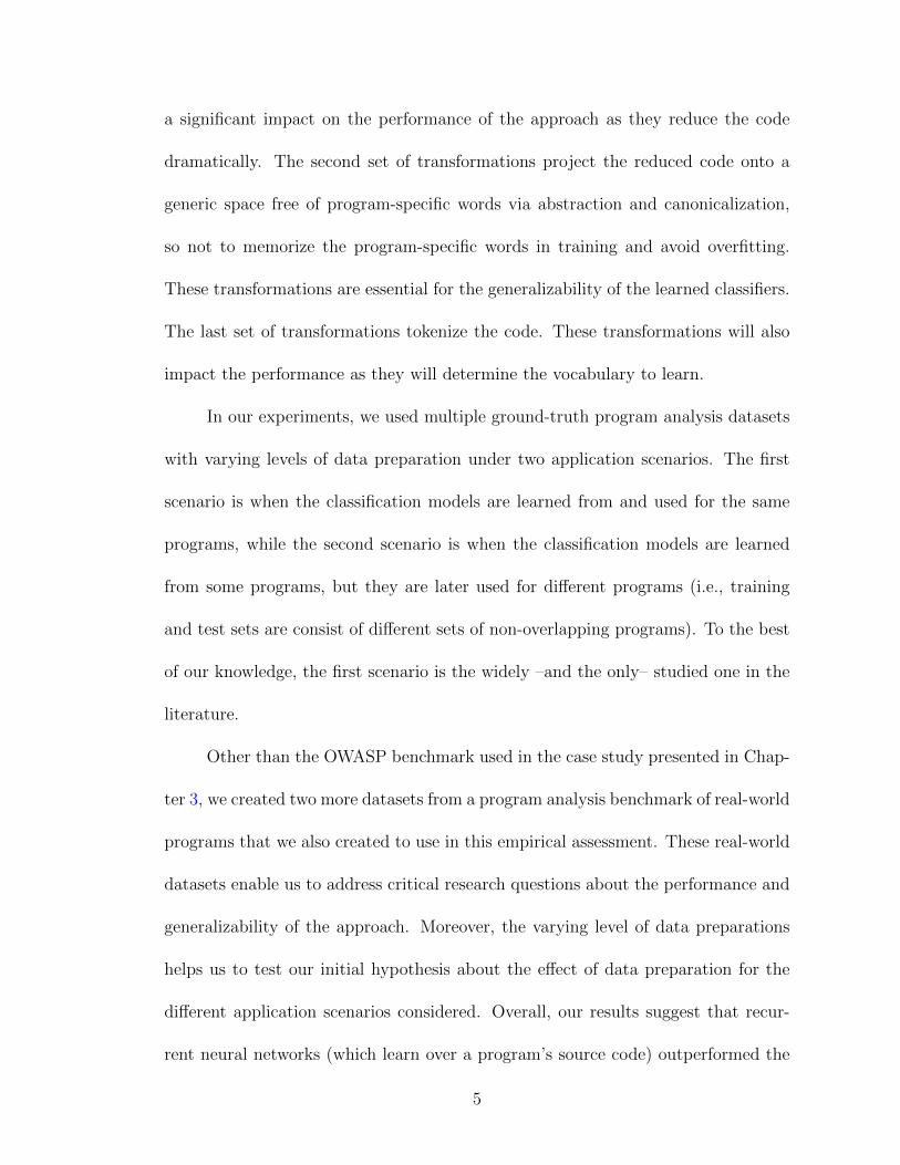
a significant impact on the performance of the approach as they reduce the code
dramatically. The second set of transformations project the reduced code onto a
generic space free of program-specific words via abstraction and canonicalization,
so not to memorize the program-specific words in training and avoid overfitting.
These transformations are essential for the generalizability of the learned classifiers.
The last set of transformations tokenize the code. These transformations will also
impact the performance as they will determine the vocabulary to learn.
In our experiments, we used multiple ground-truth program analysis datasets
with varying levels of data preparation under two application scenarios. The first
scenario is when the classification models are learned from and used for the same
programs, while the second scenario is when the classification models are learned
from some programs, but they are later used for different programs (i.e., training
and test sets are consist of different sets of non-overlapping programs). To the best
of our knowledge, the first scenario is the widely –and the only– studied one in the
literature.
Other than the OWASP benchmark used in the case study presented in Chap-
ter 3, we created two more datasets from a program analysis benchmark of real-world
programs that we also created to use in this empirical assessment. These real-world
datasets enable us to address critical research questions about the performance and
generalizability of the approach. Moreover, the varying level of data preparations
helps us to test our initial hypothesis about the effect of data preparation for the
different application scenarios considered. Overall, our results suggest that recur-
rent neural networks (which learn over a program’s source code) outperformed the
5

other learning techniques, although interesting tradeoffs are present among all tech-
niques, more precise data preparation improves the generalizability of the learned
classifiers. Our results also suggest that the second application scenario presents
interesting challenges for the research field. Our observations provide insight into
the future research needed to speed the adoption of machine learning approaches in
practice (Chapter 4).
1.2 Configurability of Program Verification Tools
Recent studies have shown that configuration options indeed present tradeoffs
[19], especially when different program features are present [20, 21, 22]. Researchers
have proposed various techniques that selectively apply a configuration option to
certain programs or parts of a program (i.e., adaptive analysis), using heuristics de-
fined manually or learned with machine learning techniques [20, 23, 21, 24, 22, 25].
Although a promising research direction, these techniques are currently focused
on tuning limited kinds of analysis options (e.g., context-sensitivity). In addition,
supervised machine learning techniques have recently been used to improve the us-
ability of static analysis tools. The applications include classifying, ranking, or
prioritizing analysis results [9, 10, 26, 27, 7, 28, 29], and ranking program verifica-
tion tools based on their likelihood of completing a given task [30, 31]. However,
the configurability of program verification tools has not been considered in these
applications. We believe that focusing on automatically selecting configurations will
make verification tools more usable and allow them to better fulfill their potential.
6

Therefore, we designed and developed a meta-reasoning approach, auto-tune,
to automatically configure program verification tools for given target programs
(Chapter 5). We aim to develop a generalizable approach that can be applied for
various tools that are implemented in and targeted at different programming lan-
guages. We also aim to develop an efficient approach that can effectively search
for a desirable configuration in large spaces of configurations. Our approach lever-
ages two main ideas to achieve these goals. First, we use prediction models both
as fitness functions and incorrect result filters. Our prediction models are trained
with language-independent features of the target programs and the configuration
options of the subject verification tools. Second, we use a meta-heuristic search al-
gorithm that searches the configuration spaces of verification tools using the models
mentioned above.
Overall, auto-tune works as follows: we first train two prediction models
for use in the meta-heuristic search algorithm. We use a ground-truth program
analysis dataset that consists of correct, incorrect, and inconclusive1 analysis runs.
The first model, the fitness function, is trained on the entire dataset; the second
model, the incorrect result filter (or, for short, filter), is trained on the conclusive part
of the dataset–i.e., excluding the inconclusive analysis runs. Our search algorithm
starts with a default configuration of the tool if available; otherwise, it starts with a
random configuration. The algorithm then systematically, but non-deterministically,
alters this configuration to generate a new configuration. Throughout the search,
1An inconclusive analysis run means the tool fails to come to a judgment due to a timeout,crash, or a similar reason.
7

the fitness function and filter are used to decide whether a configuration is a good
candidate to run the tool with. The algorithm continues to scan the search space by
generating new configurations until it locates one that both meets the thresholds in
the fitness and filter functions and leads to a conclusive analysis result when run.
We consider auto-tune as a meta-reasoning approach [32, 33] because it aims
to reason about how verification tools should reason about a given verification task.
In this setting, the reasoning of a given verification tool is controlled by configura-
tion options that enable/disable certain simplifications or assumptions throughout
the analysis tasks. The ultimate goal of meta-reasoning is to identify a reasoning
strategy, i.e., a configuration, that is likely to lead to the desired verification result.
We applied auto-tune to four popular software verification tools. CBMC and
Symbiotic [34, 35] verify C/C++ programs, while JBMC [36] and JayHorn [37] verify
Java programs. We generated program analysis datasets with the ground truths
from the SV-COMP2, an annual competition of software verification that includes
a large set of both Java and C programs. We used these datasets, which contain
between 55K and 300K data points, to train prediction models (i.e., fitness functions
and false result filters) for each tool.
To evaluate the effectiveness of auto-tune, we considered two use cases. First,
to simulate the scenario when a non-expert uses a tool without a reliable default
configuration, we start auto-tune with a random configuration. Our experiments
suggest that auto-tune produces results comparable to configurations manually and
2https://sv-comp.sosy-lab.org/2019
8

painstakingly selected by program analysis experts, i.e., comp-default3. Second,
to simulate the scenario in which a tool comes with a reliable default configuration,
or is used by an expert, we start auto-tune with the comp-default configura-
tion. Our results suggest that, with regard to the competition’s scoring system,
auto-tune improves the SV-COMP performance for three out of four program ver-
ification tools we studied Symbiotic, JayHorn, and JBMC. For CBMC, auto-tune
also significantly increases the number of correct analysis runs. However, it did not
improve the competition score due to the substantial penalty for the few incorrect
results it generated (Chapter 5).
The remainder of this document is organized as follows: Chapter 2 provides
background information; Chapter 3 presents the learning approach for classify-
ing false positive analysis results with a case study; Chapter 4 presents an empirical
assessment of different machine learning techniques for classifying false positive anal-
ysis results; Chapter 5 presents the auto-tune approach with empirical evaluations;
Chapter 6 surveys the related work; Chapter 7 summarizes the conclusions; and
Chapter 8 discusses potential directions for future work.
3These are the configurations the tools used when participating the competition.
9
Chapter 2: Background Information
In this chapter we provide high-level background information on static analysis
and the machine learning algorithms we studied.
2.1 Program Analysis
Program analysis techniques aim at analyzing software programs to find useful
facts about the programs’ properties like correctness and safety. These techniques
can be divided in two categories: dynamic analysis and static analysis. Dynamic
analysis techniques execute programs to discover these facts, while static analysis
techniques use sophisticated algorithms and formal methods to analyze the code of
the programs without executing them.
Dynamic analyses, software testing techniques specifically, are widely adopted
in software development, i.e., software development companies and individual soft-
ware developers routinely perform certain kinds of testing to check properties of
their programs that are vital for security and integrity [38, 39, 40]. The situation,
however, is not the same for static analysis. Many software companies and develop-
ers have abandoned the use of static analysis tools [41, 1, 42]. The usability concerns
we highlighted in our introduction, i.e., false positives and properly configuring the
10

tools, are two of the leading causes of this situation. Although the prior research
addressing these usability concerns has had some success, the proposed approaches
themselves had limitations about generalizability and usability. Thus they have not
created a significant impact on the adoption of static analysis in industry.
The main motivation behind the approaches we present in this dissertation is
to change the situation in favor of static analysis tools by solving the mentioned
usability issues in generalizable ways. Therefore, we used sophisticated machine
learning techniques to automate key steps in our approaches.
2.2 Supervised Classification for False Positive Detection
In this section, we provide brief background information on four machine
learning approaches we studied for supervised false positive classification: hand-
engineered features (HEF), bag of words (BoW), recurrent neural networks (RNN),
and graph neural networks (GNN).
HEF approaches can be regarded as the state-of-the-art classification applica-
tion for the false positive detection problem [43]. However, by design, they cannot
include the deep structure of the source code being analyzed. The other three ap-
proaches add an increasing amount of structural information as we move from BoW,
to RNN, and to GNN. To the best of our knowledge, BoW, RNN, and GNN have
not been used to solve this problem before.
In this dissertation, we frame the false positive detection as a standard bi-
nary classification problem [44]. Given an input vector ~x, e.g., a point in a high
11

dimensional space RD, the classifier produces an output y = fθ(~x), where y = 1
for false positives, y = 0 otherwise. Constructing such a classifier requires defining
an input vector ~x that captures features of programs that might help in detecting
false positives. We also need to select a function fθ, as different families of functions
encode different inductive biases and assumptions about how to predict outputs for
new inputs. Once these two decisions have been made, we can train the classifier
by estimating its parameters θ from a large set of known false positives and true
positives; i.e., {(x1, y1) . . . (xN , yN)}.
2.2.1 Hand-engineered Features
A feature vector ~x can be constructed by asking experts to identify measur-
able properties of the program and analysis report that might be indicative of true
positives or false positives. Each property can then be represented numerically by
one or more elements in ~x. Hand-engineered features have been defined to classify
false positive static analysis reports in existing work [45, 46, 9, 10].
Tripp et al. [10] identified lexical, quantitative, and security-specific features to
filter false cross-site scripting (XSS) vulnerability reports for JavaScript programs.
Note that identifying these features requires expertise in web application security
and JavaScript programming language. Later in Chapter 4.1.1, we describe our
adaptation of this work.
12

2.2.2 Bag of Words
How can we represent a program as a feature vector that contains useful infor-
mation to detect false positives? We take inspiration from text classification prob-
lems, where classifier inputs are natural language documents, and “Bag of Words”
(BoW) features provide simple yet effective representations [47]. BoW represents a
document as a multiset of the words found in the document, ignoring their order.
The resulting feature vector ~x for a document has as many entries as words in the
dictionary, and each entry indicates whether a specific word exists in the document.
BoW has been used in software engineering research as an information re-
trieval technique to solve problems such as duplicate report detection [48], bug
localization [49], and code search [50]. Such applications often use natural language
descriptions provided by humans (developers or users). To our knowledge, BoW has
not been used to classify analysis reports.
2.2.3 Recurrent Neural Networks
BoW features ignore the order. For text classification, recurrent neural net-
works [51, 52] have emerged as a powerful alternative approach that views the text
as an (arbitrary-length) sequence of words and automatically learns vector repre-
sentations for each word in the sequence [47].
RNNs process a sequence of words with arbitrary-lengthX = 〈x0, x1, . . . , xt, . . . , xn〉
from left to right, one position at a time. In contrast to standard feedforward neu-
ral networks, RNNs have looping connections to themselves. For each position t,
13

RNNs compute a feature vector ht as a function of the observed input xt, and the
representation learned for the previous position ht−1, i.e., ht = RNN(xt, ht−1). Once
the sequence has been read, the output vectors 〈h0, h1, . . . , hn〉 can be combined in
certain ways (e.g., mean pooling) to create a vector representation to be used for
supervised classification with a standard machine learning algorithm.
During training, the parameters of the classifier and the parameters of the
RNN function are estimated jointly. As a result, the vectors ht can be viewed as
feature representations for xt that are learned from data, implicitly capturing rele-
vant context knowledge about the sequence prefix 〈x0, . . . xt−1〉 due to the structure
of the RNN. Unlike HEF or BoW, the feature vectors ht are directly optimized for
the classification task. This advantage comes at the cost of reduced interpretability
since the values of ht are much harder for humans to interpret than the BoW or
HEF.
Figure 2.1: Structure of a standard recurrent neural network (RNN)
Figure 2.1 shows a standard RNN unit. The blue circle is the input token
xt, the yellow box is the tanh activation function, and the purple circle is the
output value ht for xt. However, researchers have noted that this RNN structure
suffers from the vanishing and exploiting gradient problems [53]. Very simply, these
problems occur during the error back-propagation, specifically with RNNs because
14
of the recurrent connection (how fθ uses ht−1).
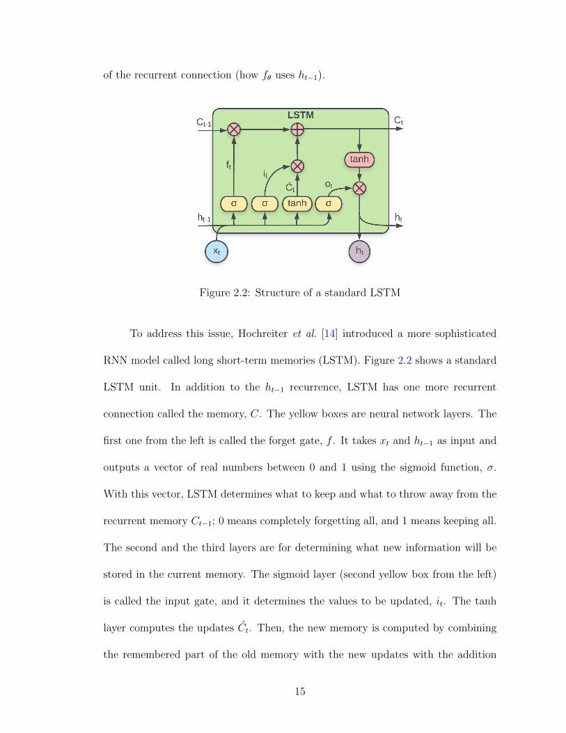
Figure 2.2: Structure of a standard LSTM
To address this issue, Hochreiter et al. [14] introduced a more sophisticated
RNN model called long short-term memories (LSTM). Figure 2.2 shows a standard
LSTM unit. In addition to the ht−1 recurrence, LSTM has one more recurrent
connection called the memory, C. The yellow boxes are neural network layers. The
first one from the left is called the forget gate, f . It takes xt and ht−1 as input and
outputs a vector of real numbers between 0 and 1 using the sigmoid function, σ.
With this vector, LSTM determines what to keep and what to throw away from the
recurrent memory Ct−1; 0 means completely forgetting all, and 1 means keeping all.
The second and the third layers are for determining what new information will be
stored in the current memory. The sigmoid layer (second yellow box from the left)
is called the input gate, and it determines the values to be updated, it. The tanh
layer computes the updates Ct. Then, the new memory is computed by combining
the remembered part of the old memory with the new updates with the addition
15

operation following the tanh. The last σ layer computes the output value, which
will be merged with the updated memory with a tanh function as the final output
value ht. Thanks to the forget gate and memory components, LSTM is capable
of capturing long-term dependencies in sequential data, and it does not have the
vanishing and exploiting gradients problem.
Various versions of RNNs, including the LSTM, are commonly used in natural
language processing (NLP) tasks such as predicting the upcoming word in typed
text [54, 55] and machine translation [56], where feature vectors ht capture syntax
and semantic information about words based on their usage in context [14, 52].
Recently, researchers have begun to use LSTMs to solve software engineering tasks
such as code completion [57], and code synthesis [58, 59]. To our knowledge, RNNS
have not been used to classify analysis reports.
2.2.4 Graph Neural Networks
With RNNs, we can represent programs as a sequence of tokens. However,
programs actually have a more complex structure that might be better represented
with a graph. To better represent structure, we explore graph neural networks
which compute vector representations for nodes in a graph using information from
neighboring nodes [60, 61]. The graphs are of the form G = 〈N,E〉, where N =
n0, n1, . . . , ni is the set of nodes, and E = e1, e2, . . . , ej is the set of edges. Each
node ni is represented with a vector hi which captures learned features of the node
in the context of the graph.
16

The edges are of the form e = 〈type, source, dest〉, where type is the type
of the edge; and source and dest are the IDs of the source and destination nodes,
respectively. The vectors hi are computed iteratively, starting with arbitrary values
at time t = 0, and incorporating information from neighboring nodes NBR(ni) at
each time step t, i.e., h(t)i = f(ni, h
(t−1)NBR(ni)
).
17
Chapter 3: Learning a Classifier for False Positive Error Reports
Emitted by Static Analysis Tools
Static Code Analyzer
Source Code
Bug Reports
Reduced Code
Learning from Code
Preprocessing
FalsePositiveReportFilter
Code Patterns
Labeling Reports
Code Reduction
In
Out
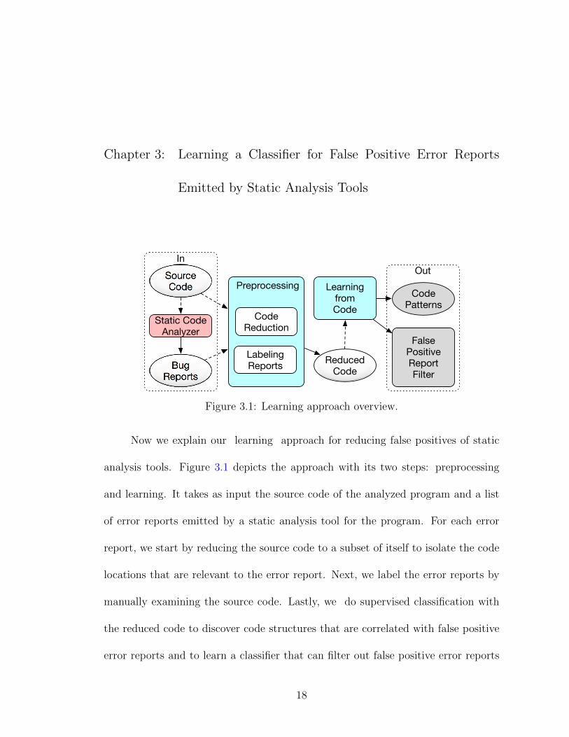
Figure 3.1: Learning approach overview.
Now we explain our learning approach for reducing false positives of static
analysis tools. Figure 3.1 depicts the approach with its two steps: preprocessing
and learning. It takes as input the source code of the analyzed program and a list
of error reports emitted by a static analysis tool for the program. For each error
report, we start by reducing the source code to a subset of itself to isolate the code
locations that are relevant to the error report. Next, we label the error reports by
manually examining the source code. Lastly, we do supervised classification with
the reduced code to discover code structures that are correlated with false positive
error reports and to learn a classifier that can filter out false positive error reports
18

emitted by the static analysis tool in the future.
3.1 Code Preprocessing
In initial work [62], we manually identified 14 core code patterns that lead to
false positive error reports. We observed that in all code patterns, the root cause
of the false error report often spans over a small number of program locations. To
better document these patterns, we performed manual code reduction to remove the
parts of the code that are not relevant for the error report, i.e., the parts that do
not affect the analysis result. After this manual reduction, the resulting program is
effectively the smallest code snippet that still leads to the same false positive error
report from the subject static analysis tool.
In this work, we develop approaches to automate the code reduction step.
Such reduction is crucial because code segments that are not relevant to the error
report may introduce noise, causing spurious correlations and over-fitting. Now, we
explain the reduction techniques we apply in the case study described in Section 3.3:
method body and program slicing.
Method body. As a naive approach, we simply took the body of the method that
contains the warning line in it (referred to as “warning method” later in the text).
Note that, many of the code locations relevant for the error report are not inside the
body of the warning method. In many cases, the causes of the report span multiple
methods and classes. Hence, this reduction is not a perfect way of isolating relevant
code locations. However, if we can detect patterns in such sparse data, our models
19

are likely to be on the right track.
Program slicing. Given a certain point in a program, program slicing is a tech-
nique that reduces that program to its minimal form, called a slice, whose execution
still has the same behavior at that point [63]. The reduction is made by remov-
ing the code that does not affect the behavior at the given point. Computing the
program slice from the warning line up to the entry point of a program would give
us a backward slice which covers all code locations that are relevant for the error
report (in theory). In practice, slicing can be expensive. We will explain how we
configured an industrial scale framework, WALA [64], for computing the backward
slice later in Section 3.3 with more detail.
3.2 Learning
Filtering false positive error reports can be viewed as a binary classification
problem with the classes True Positive and False Positive. In this binary classifi-
cation problem, we have two primary goals; 1) discovering code structures that are
correlated with these classes, and 2) learning a classifier to detect false positive er-
ror reports (see Figure 3.1). Towards achieving these goals, we explore two different
learning approaches. First, we use a simple Naive Bayes inference-based learning
model. Second, we use a neural network-based language model called LSTM [14].
The first approach is simple and interpretable. The second approach is more sophis-
ticated and it can learn more complex patterns in the data.
Naive Bayesian Inference. We formulate the problem as calculating the probabil-
20

ity that an error report is either a true positive or a false positive, given the analyzed
code. So, the probability of the error report being a false positive is P (e=0|code)
where e=0 means there is no error in the code, i.e., the error report is a false pos-
itive. Since there are only two classes, the probability of being a true positive can
be computed as P (e=1|code) = 1− P (e=0|code).
To calculate the probability P (e=0|code), we use a simple Bayesian inference:
P (e = 0|code) =P (code|e = 0)P (e = 0)
P (code)
=P (code|e = 0)P (e = 0)
P (code|e = 0)P (e = 0) + P (code|e = 1)P (e = 1)
Where P (e=0) and P (e=1) are respectively the percentages of false positive and true
positive populations in the dataset, and P (code) is the probability of getting this
specific code from the unknown distribution of all codes. To calculate P (code|e=0)
and P (code|e=1), we formulate the code as a sequence of instructions (bytecodes),
i.e., code=< I1, I2, I3, ..., In >. So we rewrite P (code|e=0) as,
P (code|e = 0) = P (I1, I2, ..., In|e = 0)
= P (I1|e = 0)P (I2, ..., In|I1, e = 0)
= P (I1|e = 0)P (I2|I1, e = 0)P (I3, ...In|I1, I2, e = 0)
...
= P (I1|e = 0)P (I2|I1, e = 0)...P (In|I1, I2, ..., e = 0)
21

Algorithm 1 Computing Probabilities
1: for each code C in Dataset do2: for each instruction I in C do3: count[C.isTruePositive][I]++4: total[C.isTruePositive]++
5: for each instruction I do6: P (I|e = 1)← count[True][I]/total[True]7: P (I|e = 0)← count[False][I]/total[False]
To calculate each probability, we need to count the number of times each combina-
tion occurs in the dataset. However, for a complicated probability like
P (In|I1, I2, ..., e = 0),
we need to have a huge dataset to be able to estimate it accurately. To avoid
this issue, we simplify this probability by assuming a Markov property. For this
analysis, the Markov property means that the probability of seeing each instruction
is conditionally independent (i.e., conditioned on e) of any other instruction in the
code. Although this assumption is not likely to be true for flow-sensitive properties of
code, it still helps us build an initial model to have an intuition of what is happening
in the dataset (our second model does not need this assumption). With the Markov
property, the underlying probability becomes:
P (code|e = 0) = P (I1|e = 0)P (I2|e = 0)...P (In|e = 0)
Calculating each of the P (Ii|e=0) is very straightforward. We count the num-
ber of times instruction Ii appears in any false positive example, and we divide it by
22

the total number of instructions in all of the false positive examples. Algorithm 1
shows how to calculate these probabilities. Line 3 counts the number of times each
instruction appears in true positive and false positive examples. Then, line 4 counts
the total number of instructions in each class. Finally, lines 8 and 9 compute the
probabilities for instructions.
Long Short Term Memory (LSTM). Here, we took inspiration from the senti-
ment analysis problem in natural language processing. Sentiment analysis is com-
monly framed as a binary classification problem with classes positive and negative,
like we did for our problem in this study. To benefit from neural network models
that a proven to be effective for the sentiment analysis problem, we convert pro-
grams into sequence of tokens. Then for a given sequence, that is the reduced code
version of a program, we want to predict a label. We think LSTM is a good fit for
this task because programs have long-term dependencies. For examples, variable
def-use pairs, method calls with arguments, and accessing class fields are some of
the program structures which would form long-term dependencies in code. These
dependencies are often relevant in deciding whether or not an error report is a false
positive.
Carrier et al.[65] designed a single layer LSTM model for the sentiment anal-
ysis problem. In this work, we adopt this simple LSTM model using the adadelta
optimization algorithm [66]. To be able to make some observations by visualizing
the inner workings of the model, we prefer having fewer (four) cells, each of which is
an LSTM (see Figure 3.4). Finding the optimum number of cells is not in the scope
of this work. Following the LSTM layer, there is a mean pooling layer to compute
23

Figure 3.2: The LSTM model unrolled over time.
a general representation of the input sequence. Finally, we do logistic regression to
classify the data into one of the two classes. Figure 3.2 shows the structure of the
LSTM unrolled over time, with n being the length of the longest sequence.
3.3 Case Study
This section presents the case study we conducted to evaluate the effectiveness
of the proposed approach.
3.3.1 Subject Static Analysis Tool and Warning Type
In this case study, we focus on the SQL (Structured Query Language) injection
flaw type. As the subject static analysis tool, we use the FindSecBugs plug-in of
FindBugs [12, 67] (a widely-used security checker for Java). This plug-in performs
taint analysis to find SQL injection flaws. Very simply, taint analysis checks for
data-flow from untrusted sources to safety-critical sink points (see Appendix A for
24

more detailed description of taint analysis). For example, one safety-critical sink
point for SQL injection is the Connection.execute(String) Java statement. A
string parameter passed to this method is considered as tainted if it comes from
an untrusted source such as an HTTP cookie or a user input (both are untrusted
sources because malicious users can leverage them to attack a system). FindSecBugs
emits an SQL injection report in such cases to warn the user of a potential security
problem.
However, for complex source code, it may be challenging to determine whether
or not a given parameter is tainted. For example, programs may receive user input
that becomes a part of an SQL query string (see Appendix A for an example). In
such cases, the best practice is to perform security checks against an injection threat
in the code. Such checks are often called sanitization or neutralization. When the
chain of information flow becomes too complicated, the static analysis tool may not
be able to track the sanitization correctly and might, therefore, emit a false positive
error report.
Note that, the proposed approach is not restricted to SQL injection flaws,
FindSecBugs, or taint analysis. They are just the focus of this case study. Our
learners do not make use of any information that is specific to these factors. Fur-
thermore, in the next chapter, we will show that it can be possible to train a model
that works for multiple flaw types or static analysis tools (see Chapter 4).
25

1 public class BenchmarkTest16536 extends HttpServlet {
2 @Override
3 public void doPost(HttpServletRequest request){
4 String param = "";
5 Enumeration<String> headers = request.getHeaders("foo");
6 if (headers.hasMoreElements()) {
7 param = headers.nextElement();
8 }
9 String bar = doSomething(param);
10 String sql = "{call verifyUserPassword(‘foo’,‘" + bar + "’)}";
11 Connection con = DatabaseHelper.getConnection();
12 con.prepareCall(sql).execute(); // A false positive SQLi warning
13 } // end doPost
14 private static String doSomething(String param){
15 String bar = "safe!";
16 HashMap<String,Object> map = new HashMap();
17 map.put("keyA", "a_Value");
18 map.put("keyB", param.toString());
19 map.put("keyC", "another_Value");
20 bar = (String) map.get("keyB");
21 bar = (String) map.get("keyA");
22 return bar;
23 } /* end doSomething*/
24 } /* end class*/
Figure 3.3: An example Owasp program that FindSecBugs generates a false positiveerror report for (simplified for presentation).
3.3.2 Data
One of the biggest challenges for our problem is to find a sufficient dataset on
which to train. We know of no publicly available benchmark datasets containing real-
world programs with labeled error reports emitted by static analysis tools. However,
there are at least two benchmark suites developed to evaluate the performance
of static analysis tools; Juliet [68] and Owasp benchmark [13]. These benchmark
suites consist of programs that exercise common weaknesses [69]. Note that not all
programs in the benchmark suites really have an actual weakness. Roughly half of
26

the programs are designed in certain ways that may trick static analysis tools into
emitting false reports. For this case study, we focused on the Owasp benchmark
suite as it has a bigger dataset for the SQL injection flaw type. This dataset has
2371 data points; 1193 false positive and 1178 true positive error reports.
Figure 3.3 shows an example Owasp program for which FindSecBugs generates
an error report. At line 7, the param variable gets a value from an HTTP header
element, which is considered to be a tainted source. The param variable is then
passed to the doSomething method as an argument. In the doSomething method,
starting at line 14, the tainted param argument is put into a HashMap object (line
18). Next, it is read back from the map into the bar variable at line 20. At this
point, the bar variable has a tainted value. However, the program then gets a new
value from the map, which is this time a hard-coded string, i.e., a trusted source.
Finally, doSomething returns this hard-coded string, which gets concatenated into
the sql variable at line 10. Then a callable statement is created and executed (lines
11 and 12). To summarize, the string concatenated with the SQL is hard-coded and
thus does not represent an injection threat. Therefore, the error report is a false
positive.
3.3.3 Preprocessing
For simplicity, we focus on the bytecode representation of the programs. With
bytecode, there are fewer program-specific tokens and syntactic components than
that found in source code, making it much easier to work on for a classification
27

model. In contrast, in the source code, there might be multiple instructions in a
single line, and what each instruction is doing is, therefore, less easy to understand.
For the SQL injection dataset, we applied the two code reduction techniques
(described in Section 3.1), leading to two different reduced datasets called “method
body” and “backward slice” respectively. Application of method body reduction is
straightforward; we simply take the bytecode for the body of the warning method.
Next, we describe the implementation details of the backward slice technique.
Tuning WALA. We use the WALA [64] program analysis framework for computing
the backward slice with respect to a warning line. In theory, this slice should cover
all code locations related to the error report. However, program slicing is unsolvable
in general and not scalable most of the time [63]. In fact, we experienced excessive
execution times when computing backward slices even for the simple short Owasp
programs. To avoid this problem, we configured the WALA program slicer to narrow
the scope and limit the amount of analysis it does for computing the slice.
First, we restricted the set of data dependencies by ignoring exception objects,
base pointers, and heap components. We assume that exception objects are not
relevant to the error report. Base pointers and heap variables, on the other hand, are
just represented as indexes in the bytecode, over which our models cannot adequately
handle, so we discarded them.
Second, we set the entry points as close to the warning method as possible. An
entry point is usually where a program starts to execute. Therefore it is the place
where the backward slice should end. By default, this point would be the main
method of the program. For the Owasp suite, however, there is a large amount of
28

code in the main method that is common for all programs. Since this shared code
is unlikely to be relevant to any error reports, we rule it out by setting the warning
method as the entry point for Owasp.
Third, we exclude Owasp utility classes, Java classes, and all classes of third
party libraries as none of them are relevant to the error report for this case study.
With this exclusion, we are not removing the references to these classes. Instead, we
are treating them as a black box. With the WALA tuning mentioned here, we are
now able to compute a modified backward slice for Owasp programs in reasonable
times.
Note that, although WALA analyzes bytecode, the slice it outputs differs
from bytecode with a few points. For presentation purposes, WALA uses some
additional instructions like new, branch, return, which do not belong to Java byte-
code1. Therefore, the dictionaries of the method body dataset and the backward
slice dataset are not the same.
Now, we explain the further changes we performed for both datasets. First of
all, we removed program-specific tokens and literal expressions because they may
give away whether the error report is a true positive or a false positive. For the
LSTM Classifier, we do this by deleting literal expressions and replacing program-
specific objects with UNK OBJ and method calls with UNK CALL. For the Naive Bayes
Classifier, we do so by simply removing them all. Note that, this step is also neces-
sary to be able to generalize the classifier across programs. If we let the model learn
from program-specific components, then it will not be able to do a good job on the
1These instructions appear in WALA IR (intermediate representation)
29

code that does not share the same ingredients.
Lastly, for the Naive Bayes Classifier, we remove all arguments to instructions
except the invoke instructions (invokeinterface, invokevirtual, etc.). With the
invoke instructions, we also keep the names of invoked classes. This is done to further
simplify the dataset. Furthermore, we treat all kinds of invoke instructions as the
same by simply replacing them with invoke. For the LSTM Classifier, we tokenized
the data by whitespace, e.g., with the invoke instructions, the instruction itself is one
token and the class being invoked is one token. Therefore, when analyzing results,
we use the word ‘token’ for LSTM and ‘instruction’ for Naive Bayes.
3.4 Results and Analysis
For all experiments, we randomly split the dataset into an 80% training set
and a 20% test set. Table 3.1 summarizes the results. Accuracy is the percentage
of correctly classified samples. Recall is the percentage of correctly classified false
positive samples in all false positive samples, and the precision is the percentage of
samples classified as false positive. All three of the metrics are computed using the
test portion of the datasets.
Training (%)Classifier dataset Time (m) Recall Precision Accuracy
Naive Bayesmethod body 0.02 60 64 63backward slice 0.03 66 75 72
LSTMmethod body 17 81.3 97.3 89.6backward slice 18 97 78.2 85
Table 3.1: Performance results for Naive Bayes and LSTM.
30

3.4.1 Naive Bayes Classifier Analysis
For the analysis of results, we consider any instruction I to be independent of
SQL injection flaw if the value
[P (I|e = 0)
P (I|e = 0) + P (I|e = 1)− 0.5
]
is smaller than 0.1 in magnitude. We call this value “False Positive Dependence”,
and it ranges from −0.5 to 0.5 inclusive, where large positive values mean the in-
struction is correlated with the false positive class. Large negative values mean it
is correlated with the true positive class. Values around zero mean the instruc-
tion is equally likely to appear in both true positive and false positive classes (i.e.,
P (I|e=0) ' P (I|e=1)) and therefore is independent of SQL injection flaw.
We started the experiment by running the Naive Bayes Classifier on the
method body dataset. Although the accuracy result is not very high for this ex-
periment (63%, in Table 3.1), it confirmed that the bytecode contains recognizable
signals indicating false positive error reports.
The Naive Bayes Classifier learns the conditional property of each instruction,
given that an error exists. We observed that instructions like iload, ifne, etc.,
are equally likely to appear in both true and false positive samples. Therefore,
their “False Positive Dependence” value is below the threshold (0.1), and these
instructions are independent of SQL injection flaws.
Next, the only instruction we found to be correlated with the false positive class
31

is invoke java.util.HashMap (Table 3.2). By manually examining the Owasp suit,
we see that, it is a common pattern to insert a tainted string and also a safe string
into a HashMap, and then extract the safe string from the HashMap to become a
part of an SQL statement (see Figure 3.3 for an example). This is done to “trick”
static analysis tools into emitting incorrect reports, and the Naive Bayes Classifier
correctly identifies this situation.
For the second experiment, we did the same analysis for the backward slices
dataset. We hypothesize that analyzing the code outside the method body improves
the effectiveness of learning. Therefore, we need to consider all relevant instructions,
even if they are outside the method body. Backward slices provide this information
by including all instructions in the program that may be relevant to the error report.
InstructionsFalse Positive Dependence
Method body Backward sliceinvoke esapi.Encoder −0.09 −0.36invoke java.util.ArrayList 0.04 0.18invoke java.util.HashMap 0.18 0.25
Table 3.2: Important instructions for classification
Running the Naive Bayes model on the backward slice dataset confirms our
findings in the method body dataset. In addition to HashMap, this model also
learns from the backward slices that ArrayList invocation is highly correlated with
false positives, and Encoder invocation is highly correlated with true positives. The
False Positive Dependence for significant classes invoked is shown in Table 3.2. These
correlations can easily be justified by examining the code.
In Owasp, ArrayList is used to trick the analyzer, much like HashMap did in
32

the previous discussion. Furthermore, Encoder is mainly used in the dataset for
things like HTML encoding but not for SQL escaping. This pattern is used to trick
the analyzer into missing some true positive samples, which our model identifies as
well.
The main reason for improved results in the backward slice dataset is that
the data points in it include all relevant instructions and the irrelevant instructions,
which might act as noise, have been removed. This increases the confidence of the
classifier. Table 3.2 shows that dependence values have increased in magnitude for
backward slices, which means the classifier is more confident about the effect of
these instructions in the code.
Weaknesses. To better understand the limitations of the Bayes model, we exam-
ined some of the incorrectly classified examples. We observed that the model can
still identify the influence of each instruction correctly. However, in those examples,
multiple instructions are correlated with true positives while a single (or very few)
instruction makes the string safe. By its nature, the Naive Bayes model cannot
take into account that a single instruction is enough to make the string untainted.
The instructions are correlated with true positive class weight more when comput-
ing the overall probability and the Naive Bayes model ends up classifying the code
incorrectly.
33

Training Analysis precision (%)dataset initial after filteringmethod body 49.6 90.5backward slice 49.6 98.0
Table 3.3: Precision improvements that can be achieved by using the LSTM modelsas a false positive filter.
3.4.2 LSTM Classifier Analysis
With the LSTM classifier, we achieved 89.6% and 85% accuracy for the method
body and backward slice datasets, respectively (Table 3.1). The classifier trained on
the method body dataset is very precise, i.e., 97.3% of the error reports classified as
false positive are indeed false positives. However, it misses 18.7% of false positives,
i.e., classifying them as true positives. Using this classifier as a false positive report
filter would significantly improve the tools precision from 49.6% to 90.5% (the first
row if Table 3.3). The situation is reversed for the classifier trained on the backward
slice dataset. It catches 97% of the false positives but also filters out many true
positive reports, i.e., 21.8% of the samples classified as false positive are indeed true
positive. This translates to a greater improvement in the tools precision from 49.6%
to 98% (the second row if Table 3.3).
We examined a sample program which was correctly classified by the classi-
fier trained on the method body dataset, but incorrectly classified by the classifier
trained on the backward slice dataset. We observed that many instructions that
only exist in the method body dataset, like aload 0, i const 0, dup, etc., are found
to be important by the classifier. There may be two reasons why these instructions
are not in the backward slice dataset: either because they do not have any effect on
34

the warning line, or because of the tuning we did for WALA. The first case, learning
the instructions that are not related to the warning line, would be over-fitting the
noise. The second case, however, requires a more in-depth examination that we
defer to the future work (see Chapter 4). Just relying on the first case, we think
that the classifier trained on the backward slice dataset is more generalizable as this
dataset has lesser noise and more report relevant components. Hence, in the rest of
this section, we will only analyze the classifier trained on the backward slice dataset.
Understanding the source of the LSTM’s high performance is very challeng-
ing as we cannot fully unfold its inner workings. Nevertheless, we can visualize
the output values of some cells, as suggested by Karpathy et al. [70]. Figure 3.4
illustrates the output values of four cells for two correctly classified backward slices
by coloring the background. The latter is the slice computed for the false positive
sample in Figure 3.3. The former is the slice computed for a true positive, which is
structurally similar to the latter with two critical differences; 1) the doSomething
method is defined in an inner class, and 2) in the doSomething method HTML
encoder API methods are called instead of the HashMap operations.
If the LSTM model finds an input token important for the classification task
it will produce an output (i.e., the ht vector) that is large in magnitude. The cyan,
yellow, and white background colors in Figure 3.3 mean positive, negative, and
under threshold (±0.35) output values, respectively. There is only one shade white,
but for cyan and yellow, the darker the background, the larger the LSTM output
(ht) is (in magnitude). Note that, last tokens are the labels; “truepositive” and
“falsepositive”.
35

Now, we discuss some interesting observations from Figure 3.4. First, due to
the memory component of the LSTM, the background color of a token (output for
that token) does not solely depend on that token but is affected by the history.
For example, looking at Cell 1, the first invokeinterface token has a yellow back-
ground color in both samples. Since there is no history before the first token, this
yellowness is solely due to that token. On the other hand, looking at Cell 4, the first
lines of both samples mostly the same except that there is one token with cyan back-
ground color in the true positive sample; eq. The only difference in the first lines
is the tainted sources invoked, which are HttpServletRequest.getHeaderNames
and HttpServletRequest.getHeaders String in true positive and false positive,
respectively. Therefore, the only reason why eq token is interesting only in the true
positive sample must be the invocation of the tainted source HttpServletRequest.getHeaderNames.
This demonstrates a good example of a long-term dependency, as there are six other
tokens in between.
Second, in both samples, all cells have a high output for the Enumeration.nextElement
token, which is highly relevant for the error report as it is the tainted source. Note
that, all cells treat this token the same way in both samples. Similarly, all cells have
a very high output for the last return instructions in both samples. However, this
time, the output is negative in the true positive sample and positive in the false
positive sample (in the first three cells and vice versa for in the last cell), which
happens due to the history of tokens. This situation illustrates the LSTM’s ability
to infer the context in which these tokens appear.
Next, looking at the false positive sample in Figure 3.3, we see that the core
36

Figure 3.4: LSTM color map for two correctly classified backward slices.
reason for being a false positive resides in the body of the doSomething method.
In particular, HashMap put and get instructions are very critical. All cells have
a very high output for a subset of the tokens that correspond to that instruc-
tions. These high output values for HashMap put and get instructions match
the findings of the Bayesian model. Furthermore, all cells go very yellow for the
Encoder.encodeForHTML method call in the true positive sample. These high re-
sults for Encoder tokens are also consistent with the findings of the Bayesian model.
Lastly, Figure 3.4 shows that although most of the high output values are
reasonable and interpretable, there are still many that we cannot explain. This
situation is common with neural networks, and we will continue to explore it in
future work.
37
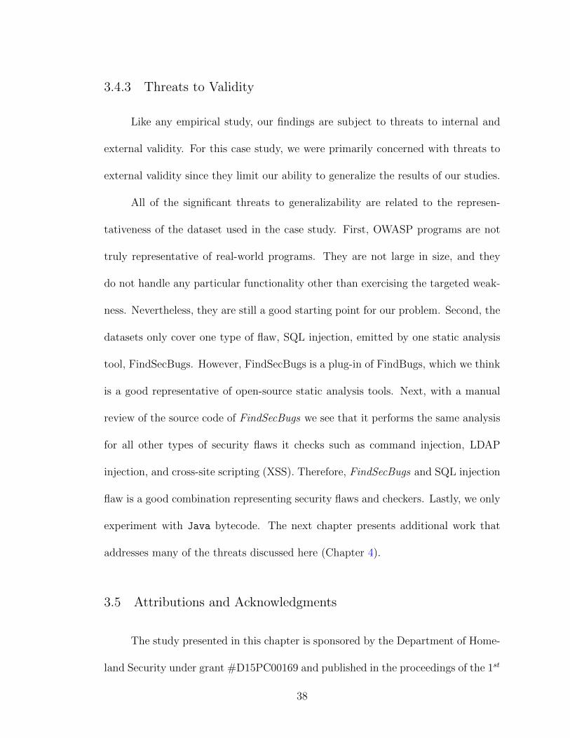
3.4.3 Threats to Validity
Like any empirical study, our findings are subject to threats to internal and
external validity. For this case study, we were primarily concerned with threats to
external validity since they limit our ability to generalize the results of our studies.
All of the significant threats to generalizability are related to the represen-
tativeness of the dataset used in the case study. First, OWASP programs are not
truly representative of real-world programs. They are not large in size, and they
do not handle any particular functionality other than exercising the targeted weak-
ness. Nevertheless, they are still a good starting point for our problem. Second, the
datasets only cover one type of flaw, SQL injection, emitted by one static analysis
tool, FindSecBugs. However, FindSecBugs is a plug-in of FindBugs, which we think
is a good representative of open-source static analysis tools. Next, with a manual
review of the source code of FindSecBugs we see that it performs the same analysis
for all other types of security flaws it checks such as command injection, LDAP
injection, and cross-site scripting (XSS). Therefore, FindSecBugs and SQL injection
flaw is a good combination representing security flaws and checkers. Lastly, we only
experiment with Java bytecode. The next chapter presents additional work that
addresses many of the threats discussed here (Chapter 4).
3.5 Attributions and Acknowledgments
The study presented in this chapter is sponsored by the Department of Home-
land Security under grant #D15PC00169 and published in the proceedings of the 1st
38

ACM SIGPLAN International Workshop on Machine Learning and Programming
Languages [71]. I, Ugur Koc, came up with the idea of learning from source code
and designed the neural network-based learning approach to realize the idea. I also
designed and conducted the LSTM experiments and analyzed the results. The devel-
opment, experimentation, and analysis tasks of the Naive Bayesian inference-based
learning approach are carried out by the collaborator Parsa Saadatpanah.
39
Chapter 4: An Empirical Assessment of Machine Learning Approaches
for Triaging Reports of a Java Static Analysis Tool
In the previous chapter, we introduced a learning approach for classifying false
positive error reports and evaluated its effectiveness with a case study of a static
analysis tool. In this case study, we experimented with a Naive Bayesian inference
model and a LSTM model, which could capture source code-level characteristics
that may have led to false positives. This evaluation showed that LSTM significantly
improved classification accuracy, compared to a Bayesian inference-based approach.
Given the limited data set involved in the case study, however, further research is
called for.
Overall, while existing research suggests that there are benefits to applying
machine learning algorithms to classify analysis results, there are important open
research questions to be addressed before these techniques are likely to be routinely
applied to this use case. First and foremost, there has been relatively little exten-
sive empirical evaluation of different machine learning algorithms for false positive
detection. Such empirical evaluation is of great practical importance for under-
standing the tradeoffs and requirements of classification techniques. Second, the
effectiveness and generalizability of the features used and data preparation tech-
40
niques needed for different classification techniques have not been well-investigated
for actual usage scenarios. Third, there is also a need for more extensive, real-world
program datasets to better validate the findings of prior work, which was primarily
conducted on synthetic benchmarks. These open problems leave uncertainty as to
which approaches to use and when to use them in practice.
To partially address these limitations, in this chapter, we describe a system-
atic, comparative study of multiple machine learning approaches for classifying static
analysis results1. Our research makes several key contributions. First, we create a
real-world, ground-truth program analysis benchmark for the experiments, consist-
ing of 14 Java programs covering a wide range of application domains and 400
vulnerability reports from a widely used static analysis tool for Java (Section 4.2).
Second, we introduce key data preparation routines for applying neural networks
to this problem (Section 4.1). Third, we compare the effectiveness of four families
of machine learning approaches: hand-engineered features, bag of words, recurrent
neural networks, and graph neural networks, with different combinations of data
preparation routines (Section 4.3).
Our experimental results provide significant insights into the performance and
applicability of the classification and data preparation techniques in two different
real-world application scenarios we studied. First, we observe that the recurrent
neural networks perform better compared to the other approaches. Second, with
more precise data preparation, we achieved significant performance improvements
1The experimental infrastructure of this study (including all raw data) is available at: https:
//bitbucket.org/ugur_koc/mangrove
41

over the state-of-the-art [71]. Furthermore, with the two application scenarios we
studied, we demonstrated that the data preparation for neural networks has a signif-
icant impact on the performance and generalizability of the approaches, and differ-
ent data preparation techniques should be applied in different application scenarios
(Section 4.4).
4.1 Adapting Machine Learning Techniques to Classify False Posi-
tives
In this section, we discuss our adaptations of the four machine learning ap-
proaches (discussed in Chapter 2) for false positive classification: hand-engineered
features (HEF), bag of words (BoW), recurrent neural networks (RNN), and graph
neural networks (GNN).
4.1.1 Hand-engineered Features
In this work, we adapted the original feature set from Tripp et al. [10]. These
features are: (1) source identifier (e.g., document.location), (2) sink identifier
(e.g., window.open), (3) source line number, (4) sink line number, (5) source URL,
(6) sink URL, (7) external objects (e.g., flash), (8) total results, (9) number of steps
(flow milestones comprising the witness path), (10) analysis time, (11) number of
path conditions, (12) number of functions, (13) rule name, (14) severity. From this
list, we dropped source URL, sink URL, and external objects as they do not ap-
pear in Java applications (our datasets consist of Java programs, Section 4.2). We
42

also extended it with two features extracted from static analysis reports that might
improve the detection of false positives: confidence of the analyzer, and number of
classes referred in the error trace (only relevant in object-oriented programming).
We conjecture that longer error traces with references to many classes might indi-
cate imprecision in the analysis, thus suggesting a higher chance of false positives.
The confidence is nominal numeric value determined by the static analysis tool rep-
resenting the internal robustness of the analysis conducted to generate the error
report.
Once the feature representations are defined, a wealth of classifiers fθ and
training algorithms can be used to learn how to make predictions. Since feature
vectors ~x encode rich knowledge about the task, classifiers fθ that compute sim-
ple combinations of these features can be sufficient to train good models quickly.
However, defining diverse features that capture all variations that might occur in
different datasets is challenging and requires human expertise.
Next, we explore how to represent program source code for more sophisti-
cated machine learning approaches that can implicitly learn feature representations,
starting with explaining how we summarized programs as a preprocessing step for
them.
4.1.2 Program Slicing for Summarization
BoW, LSTM, and GNN approaches work directly on the content of programs
being analyzed, i.e. source code. Real-world programs are large (see Table 4.1),
43

and learning directly from such data is challenging since many sections of the code
are unlikely to pertain to false positives and are likely to introduce noise for certain
classification techniques. To address this difficulty, we computed the backward slice
in the case study as shown in Chapter 3 [71]. The rationale for this choice is that
the backward slice is a good summary of programs for the static analysis report
classification task as it includes all the statements that may affect the behavior at
the reported line.
We use backward slice as well, as a pre-summarization step for BoW, RNN,
and GNN approaches. In contrast to the case study in Chapter 3, in this work, we
used Joana [72], a program analysis framework for Java, for computing backward
slices. The first step is determining the entry points from which the program starts
to run. For our problem, we first find the call hierarchy of the method containing
the error line, then in this hierarchy, identify the methods that can be invoked by
the user to set as the entry points. Such methods can be APIs if the program is a
library, or the main method (which is the default entry point), or test cases. Next,
we compute the program dependency graph (PDG), which consists of PDG nodes
denoting the program locations that are reachable from the entry points. Then,
we identify the PDG node(s) that appear in the reported source line. Finally, we
compute the backward slice as a subgraph of the PDG by finding all the paths from
the PDG nodes at the reported line to the entry point(s).
Figure 4.1 shows an example PDG node. Line 1 shows the kind and ID of the
node, which are EXPR and 164, respectively. At line 2, we see that the operation is a
44
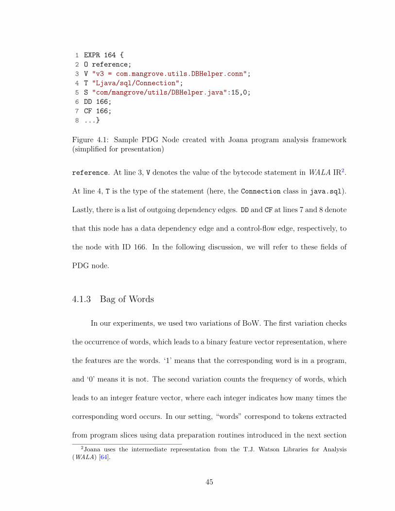
1 EXPR 164 {
2 O reference;
3 V "v3 = com.mangrove.utils.DBHelper.conn";
4 T "Ljava/sql/Connection";
5 S "com/mangrove/utils/DBHelper.java":15,0;
6 DD 166;
7 CF 166;
8 ...}
Figure 4.1: Sample PDG Node created with Joana program analysis framework(simplified for presentation)
reference. At line 3, V denotes the value of the bytecode statement in WALA IR2.
At line 4, T is the type of the statement (here, the Connection class in java.sql).
Lastly, there is a list of outgoing dependency edges. DD and CF at lines 7 and 8 denote
that this node has a data dependency edge and a control-flow edge, respectively, to
the node with ID 166. In the following discussion, we will refer to these fields of
PDG node.
4.1.3 Bag of Words
In our experiments, we used two variations of BoW. The first variation checks
the occurrence of words, which leads to a binary feature vector representation, where
the features are the words. ‘1’ means that the corresponding word is in a program,
and ‘0’ means it is not. The second variation counts the frequency of words, which
leads to an integer feature vector, where each integer indicates how many times the
corresponding word occurs. In our setting, “words” correspond to tokens extracted
from program slices using data preparation routines introduced in the next section
2Joana uses the intermediate representation from the T.J. Watson Libraries for Analysis(WALA) [64].
45
(Section 4.1.4).
Similar to the HEF approach, once the feature vector representations are cre-
ated, any classification algorithm can be used for training. For a fixed classifier,
training with BoW often takes longer than learning with HEF because the feature
space (i.e., the dictionary) is usually significantly larger.
4.1.4 Recurrent Neural Networks
In this study, we use the same LSTMs architecture that we used in the case
study (see Figure 3.2) [71]. However, this time, we perform more precise data
preparation with four sets of transformations. We denote each transformation as
Tx for some x so we can refer to it later. We list the transformations in order of
complexity, and a given transformation is applied only after applying all of the other,
less sophisticated transformations.
4.1.4.1 Data Cleansing and Tokenization (Tcln)
This set of transformations remove specific PDG nodes and perform basic to-
kenization. First, they remove nodes of certain kinds (i.e., formal in, formal out,
actual in, actual out), or whose value fields contain any of the phrases: many2many,
UNIQ, 〈init〉, immutable, fake, exception , or whose class loader is Primordial,
which means this class is not part of program’s source code. These nodes are re-
moved because they do not provide useful information for learning. Some of them
do not even inhibit anything from the actual content of programs, but instead they
46

are in the PDG to satisfy the static single assignment form3. For instance, the nodes
with type NORM and operation compound do not have bytecode instructions from the
program in their value field. Instead, their values contain the phrase many2many (en-
coding many-to-many connections in the PDG), which is not useful for our learning
task. Second, Tcln transformations extract tokens from paths of classes and methods
by splitting them by delimiters like ‘.’, ‘,’, ‘:’, and ‘/’.
4.1.4.2 Abstracting Numbers and String Literals (Tans)
These transformations replace numbers and string literals that appear in a
program slice with abstract values. We hypothesize that these transformations will
make learning more efficient by reducing the vocabulary of a given dataset and will
help us to train more generalizable models.
First, two-digit numbers are replaced with N2, three-digit numbers are with
N3, and numbers with four or more digit are with N4+. We apply similar transfor-
mations for negative numbers and numbers in scientific notation. Next, we extract
the list of string literals and replace each of them with the token STR followed by a
unique number. For example, the first string literal in the list will be replaced with
STR 1.
3A property of the representation which requires that each variable is assigned exactly once,and every variable is defined before it is used [73].
47

4.1.4.3 Abstracting Program-specific Words (Taps)
Many programmers use a common, small set of words as identifiers, e.g., i,
j, and counter are often used as integer variable identifiers. We expect that such
commonplace identifiers are also helpful for our learning task. On the other hand,
programmers might use identifiers that are program or domain-specific, and hence
do not commonly appear in other programs. Learning these identifiers may not be
useful for classifying static analysis reports in other programs.
Therefore, Taps abstracts away certain words from the dataset that occur less
than a certain amount of time, or that only occur in a single program, by replacing
them with phrase UNK. Similar to Tans, these transformations are expected to
improve the effectiveness and generalizability by reducing the vocabulary size via
abstractions.
4.1.4.4 Extracting English Words From Identifiers (Text)
Many identifiers are composed of multiple English words. For example, the
getFilePath method from the Java standard library consists of three English words:
get, File, and Path. To make our models more generalizable and to reduce the
vocabulary size, we split any camelCase or snake case identifiers into their con-
stituent words. Doing so, we increase the shared components of different programs
as many of the extracted words are very commonplace in programming, like ‘get’ in
the example above. Reducing rather less commonplace identifiers to such basic and
common tokens will also help us learn more generalizable models.
48

Although in our case study [71], we have used transformations similar to Tcln,
Tans, and Taps, to the best of our knowledge, the effects of these transformations
have not been thoroughly studied before. This study partially addresses this knowl-
edge gap with the systematic experiments we conducted with varying levels of data
preparation (Section 4.3). Moreover, in this study, we further improved and ex-
tended the transformations for mapping string literals and numbers with generic
placeholders (e.g., STR 1, N1), splitting paths of classes and methods, and removing
certain PDG nodes to improve the effectiveness and generalizability.
4.1.5 Graph Neural Networks
In our study, we focus on a variation of GNNs called Gated Graph Neural
Networks (GGNN) [74]. GGNNs have gated recurrent units and enable the initial-
ization of the node representation. GGNNs have been used to learn properties about
programs [74, 75], but have not been applied to classify static analysis reports or to
learn from program slices.
GGNNs require a fixed length vector to represent the graph nodes, i.e., the
PDG node in our problem. PDG nodes, however, have arbitrary length informa-
tion, mostly due to their ‘Value’ field, which holds the actual bytecode instruction.
Therefore, creating a fixed length vector that captures all information available in
the PDG node is a challenge. To adapt GGNNs to our problem, we introduce three
approaches for initializing the input node representations ni.
49
4.1.5.1 Using Kind, Operation, and Type Fields (KOT)
As the first representation, we only use the Kind, Operation, and Type fields of
the PDG nodes. For the example node in Figure 4.1, the KOT node representation
is Vrep =[EXPR, reference, Ljava/sql/Connection].
4.1.5.2 Extracting a Single Item in Addition to KOT (KOTI)
In the second representation, in addition to KOT, we include one more item
that usually comes from the Value field of the PDG node depending on the Operation
field. For example, if the operation is call, or entry, or exit, we extract the iden-
tifier of the method that appears in the statement. The KOTI representation for
the PDG node in Figure 4.1 is Vrep =[EXPR, reference, Ljava/sql/Connection,
object] (object is the extracted item, meaning that the reference is for an object).
4.1.5.3 Node Encoding Using Embeddings (Enc)
In the third representation, we use word embeddings to compute a vector
representation that accounts for the entire bytecode in the Value field (which has
an arbitrary number of words). To achieve this, we first perform pre-training using
a bigger, unlabeled dataset to learn embedding vectors that capture more generic
aspects of the words in the dictionary using the word2vec model [76, 77]. Then we
take the average of the embedding vectors of the words that appear in the Value
field as its representation, EV . Finally, we create a node vector by concatenating
50

EV with the embedding vectors of Kind, Operation, and type, i.e.,
Vrep = EK ++ EO ++ ET ++ EV
where ++ is the concatenation operation.
4.2 Tool and Benchmarks
Here, we explain the static analysis tool and corresponding ground-truth bench-
marks we collected to empirically compare the effectiveness of the machine learning
approaches.
The static analysis tool we study is FindSecBugs [12] (version 1.4.6), a popular
security checker for Java web applications. We configured FindSecBugs to detect
cross-site scripting (XSS), path traversal (XPATH), and SQL, command, CRLF,
and LDAP injections. We selected this subset of vulnerabilities because they share
similarities in performing suspicious operations on safety-critical resources. Such
operations are detected by the taint analysis implemented in FindSecBugs.
We used two benchmarks in our evaluation. The first is the OWASP Bench-
mark [13], which has been used to evaluate various static analysis tools in the liter-
ature [78, 79]. In particular, we used the same programs that we used in our initial
case study so that we could compare results; i.e., 2371 SQL injection vulnerability
reports, 1193 of which are false positives; the remaining reports are true positives.
We constructed the second benchmark, consisting of 14 real-world programs.
We ran FindSecBugs on these programs, and then manually labeled the resulting
51

vulnerability reports as true or false positives. We chose these programs using the
following criteria:
• We selected programs for which FindSecBugs generates vulnerability reports.
To have the kinds of vulnerabilities we study, we observe that programs should
perform database and LDAP queries, use network connections, read/write
files, or execute commands.
• We chose programs that are open source because we need access to source code
to apply our classification algorithms.
• We chose programs that are under active development and are highly used.
• Finally, we chose programs that are small to medium size, ranging from 5K
to 1M lines of code (LoC). Restricting code size was necessary to successfully
create the PDG, which is used for program slicing [72].
Table 4.1 shows the details of the programs we collected. Several programs
have been used in past research: H2-DB and Hsqldb are from the Dacapo Bench-
mark [94] (the other Dacapo programs did not satisfy our selection criteria), and
FreeCS and UPM were used by Johnson et al. [95]. These 14 programs range from 6K
to 916K LoC and cover a wide range of functionality (see the description column).
In total, the 12 programs on GitHub have a large user base with 5363 watchers,
24 723 stars, and 10 561 forks on GitHub. The other two, Freecs and HSQDB, have
41K+ and 1M+ downloads, respectively, on sourceforge.net as of October 2018.
52

# ofreports
Program Description LoC TP FPApollo-0.9.1 distributed config. management system [80] 915 602 4 6BioJava-4.2.8 computational genomics framework[81] 184 040 26 32FreeCS-1.2 chat server [82] 27 252 10 0Giraph-1.1.0 graph processing system [83] 120 017 1 8H2-DB-1.4.196 database engine [84] 235 522 17 30HSQLDB-2.4.0 database engine [85] 366 902 43 15Jackrabbit-2.15.7 content repository [86] 416 961 1 6Jetty-9.4.8 web server with servlets [87] 650 663 12 4Joda-Time-2.9.9 date and time framework [88] 277 230 2 3JPF-8.0 symbolic execution tool [89] 119 186 15 27MyBatis-3.4.5 persistence framework [90] 133 600 3 15OkHttp-3.10.0 Android HTTP client [91] 60 774 10 2UPM-1.14 password management [92] 6358 2 13Susi.AI-07260c1 artificial intellegence API [93] 65 388 47 46Total - 194 206
Table 4.1: Programs in the real-world benchmark.
Running FindSecBugs on these programs resulted in more than 400 vulnerabil-
ity reports. We then labeled the reports by manually reviewing the code4, resulting
in 194 true and 206 false positives as ground-truth. To label a static analysis report,
we first compute the backward call tree from the method that has the reported error
line. Then we inspect the code in all callers until either we find a data-flow from
an untrusted source (e.g., user input, HTTP request) without any sanity check—
indicating a true positive—or we exhaust the call tree without identifying any tainted
or unchecked data-flow—indicating a false positive.
Through this review process, we observed that the false positives we found
in the real-world benchmark were significantly different from those in the OWASP
benchmark programs. The false positives of FindSecBugs usually happen due to
4Ugur Koc performed all of the labeling work, while other collaborators verified a randomselection of labels [96].
53

one of three scenarios:
1. the tool over-approximates and incorrectly finds an unrealizable flow;
2. the tool fails to recognize that a tainted value becomes untainted along a path,
e.g., due to a sanitization routine; or
3. the source that the tool regards as tainted is actually not tainted.
In the OWASP benchmark, false positives mostly stem from the first scenario.
In our real-world benchmark, we mostly see only the second and third scenarios.
This demonstrates that the OWASP programs do not represent the diversity in the
real-world programs well enough. Therefore, creating a real-world benchmark for
our study is essential to demonstrate the generalizability of our approaches.
4.3 Experimental Setup
Applied preparations Approach nameOccurrence feature vec. BoW-OccFrequency feature vec. BoW-FreqTcln LSTM-RawTcln + Tans LSTM-ANSTcln + Tans + Taps LSTM-APSTcln + Tans + Taps + Text LSTM-ExtKind, operation, and type node vec. GGNN-KOTKOT + an extracted item GGNN-KOTINode Encoding GGNN-Enc
Table 4.2: BoW, LSTM, and GGNN approaches
In this section, we discuss our experimental setup, including the variations of
machine learning algorithms we compared, and how we divide datasets into training
and test sets to mimic two different usage scenarios.
54

Variations of Machine Learning Algorithms. We compared the four
families of machine learning approaches described in Section 4.1. For learning with
HEF, we experimented with nine classification algorithms: Naive Bayes, Bayesian-
Net, DecisionTree (J48), Random Forest, MultiLayerPerceptron (MLP), K*, OneR,
ZeroR, and support vector machines, with the 15 features described in Section 4.1.1.
We used the WEKA [97] implementations of these algorithms.
For the other three families of approaches, we experimented with the variations
described in Sections 4.1.3, 4.1.4, and 4.1.5. Table 4.2 lists these variations with their
names and data preparation applied for them. For example, the approach LSTM-
Raw uses Tcln transformations alone, while LSTM-Ext uses all four transformations.
For BoW, we only used DecisionTree (J48) based on its good performance on HEF
approaches. We adapted the LSTM implementation designed by Carrier et al. [65]
and extended a GGNN implementation from Microsoft Research [98].
Application Scenarios. In practice, we envision two scenarios for using
machine learning to classify false positives. First, developers might continuously
run static analysis tools on the same set of programs as those programs evolve over
time. For example, a group of developers might use static analysis as they develop
their code. In this scenario, the models might learn signals that specifically appear
in those programs, certain identifiers, API usage, etc. To mimic this scenario, we
divide the OWASP and real-world benchmark randomly into training and test sets.
In doing so, both training and test sets will have samples from each program in the
dataset. We refer to the real-world random split dataset as RW-Rand for short.
Second, developers might want to deploy the static analysis tool on a new
55

subject program. In this scenario, the training would be performed on one set
of programs, and the learned model would be applied to another. To mimic this
scenario, we divide the programs randomly so that a collection of programs forms
the training set and the remaining ones form the test set. To our knowledge, this
scenario has not been studied in the literature for the static analysis report classifi-
cation problem. Note that the OWASP benchmark is not appropriate for the second
scenario as all the programs in the benchmark were developed by same people and
hence share many common properties like variable names, length, API usage, etc.
We refer to the real-world program-wise split dataset as RW-PW for short.
Training Configuration. Evaluating classification techniques requires sep-
arating data points into a training set, that is used to estimate model parameters,
and a test set, that is used to evaluate classifier performance. For both scenarios, we
performed 5-fold cross-validation, i.e., five random splits for the first scenario and 5
program-wise splits for the second scenario, by dividing the dataset into five subsets
and using four subsets for training and one subset for testing, for each 4-way com-
binations. Furthermore, we repeat each execution five times with different random
seeds. The purpose of these many repetitions (5-fold cross-validation × 5 random
seeds = 25 runs) is to evaluate whether the results are consistent (see RQ3).
LSTM and GGNN are trained using an iterative algorithm that requires users
to provide a stopping criterion. We set a timeout of five hours, and we ended
training if there was no accuracy improvement for 20 and 100 epochs, respectively.
We made this choice because an LSTM epoch takes about five times longer to run
than a GGNN epoch, making this threshold approximately the same in terms of
56

clock time.
For the LSTM, we conducted small-scale experiments of 15 epochs with the
RW-Rand dataset and LSTM-Ext to determine the word embedding dimension for
tokens and batch size. We tested 4, 8, 12, 16, 20, and 50 for the word embeddings and
1, 2, 4, 8, 16, and 32 for the batch size. We observed that word embedding dimension
8 and batch size 8 led to the highest test accuracy on average, and thus we use these
values in the remaining experiments. We also used this embedding dimension for
the pre-training of GGNN-Enc.
Metrics. To evaluate the efficiency of the machine learning algorithms in
terms of time, we use the training time and the number of epochs. After loading a
learned model to the memory, the time to test a data point is negligible (around a
second) for all algorithms. To evaluate effectiveness, we use recall, precision, and
accuracy as follows:
Precision(P ) =# of correctly classified true positives
# of samples classified as true positive
Recall(R) =# of correctly classified true positives
all true positives
Accuracy(A) =# of correctly classified samples
# of all samples, i.e., size of test set
Accuracy is a good indicator of effectiveness for our study because there is no
trivial way to achieve high accuracy having an even distribution of samples for each
class. Recall can be more useful when missing a true positive report is unacceptable
(e.g., when analyzing safety-critical systems). Precision can be more useful when
the cost of reviewing false positive report is unacceptable. All three metrics are
57

computed using the test portion of the datasets.
Research questions. With the above experimental setup, we conducted our
study to answer the following research questions (RQ).
• RQ1 (overall performance comparison): Which family of approaches
perform better overall?
• RQ2 (effect of data preparation): What is the effect of data preparation
on performance?
• RQ3 (variability analysis): What is the variability in the results?
• RQ4 (further interpreting the results): How do the approaches differ
in what they learn?
All experiments were carried on a 64-bit Linux (version 3.10.0-693.17.1.el7)
VM running on 12-core Intel Xeon E312xx 2.4GHz (Sandy Bridge) processor and
262GB RAM.
4.4 Analysis of Results
In total, we trained 1350 static analysis report classification models: 3 datasets
× 5 splits × 5 random seeds × (9 algorithms for HEF + 2 BoW variations + 4 data
preparation routines for LSTM + 3 node representations for GGNN). The summary
of the results can be found in Tables 4.3 and 4.4, as the median and semi-interquartile
range (SIQR) of 25 runs. We report the median and SIQR because we do not have
any hypothesis about the underlying distribution of the data. Note that, for HEF,
58

we list the four algorithms that had the best accuracy: K*, J48, RandomForest, and
MLP. We now answer each RQ.
4.4.1 RQ1: Overall Performance Comparison
In this section, we analyze the overall performance of four main learning ap-
proaches using the accuracy metric and we observe that the trends we mention
here also hold for the recall and precision metrics. In Table 4.3, we separated high
performing approaches from others with a dashed-line at points where there is a
large gap in accuracy. Overall, LSTM-based approaches outperform other learning
approaches in accuracy. The deep learning approaches (LSTM and GGNN) classify
false positives more accurately than HEF and BoW, at the cost of longer training
times. The gap between LSTM and GGNN and other approaches is larger in the
second application scenario suggesting that the hidden representations learned gen-
eralize across programs better than HEF and BoW features. Next, we analyze the
results for each dataset.
For the OWASP dataset, all LSTM approaches achieve above 98% for recall,
precision, and accuracy metrics. BoW approaches are close, achieving about 97%
accuracy. The HEF approaches, however, are all below the dashed-line with below
80% accuracy. We conjecture that the features used by HEF do not adequately
capture the symptoms of false (or true) positive reports (see Section 4.4.4). The
GGNN variations have a big difference in accuracy. The GGNN-Enc achieves 94%,
while the other two variations achieve around 80% accuracy. This suggests that for
59
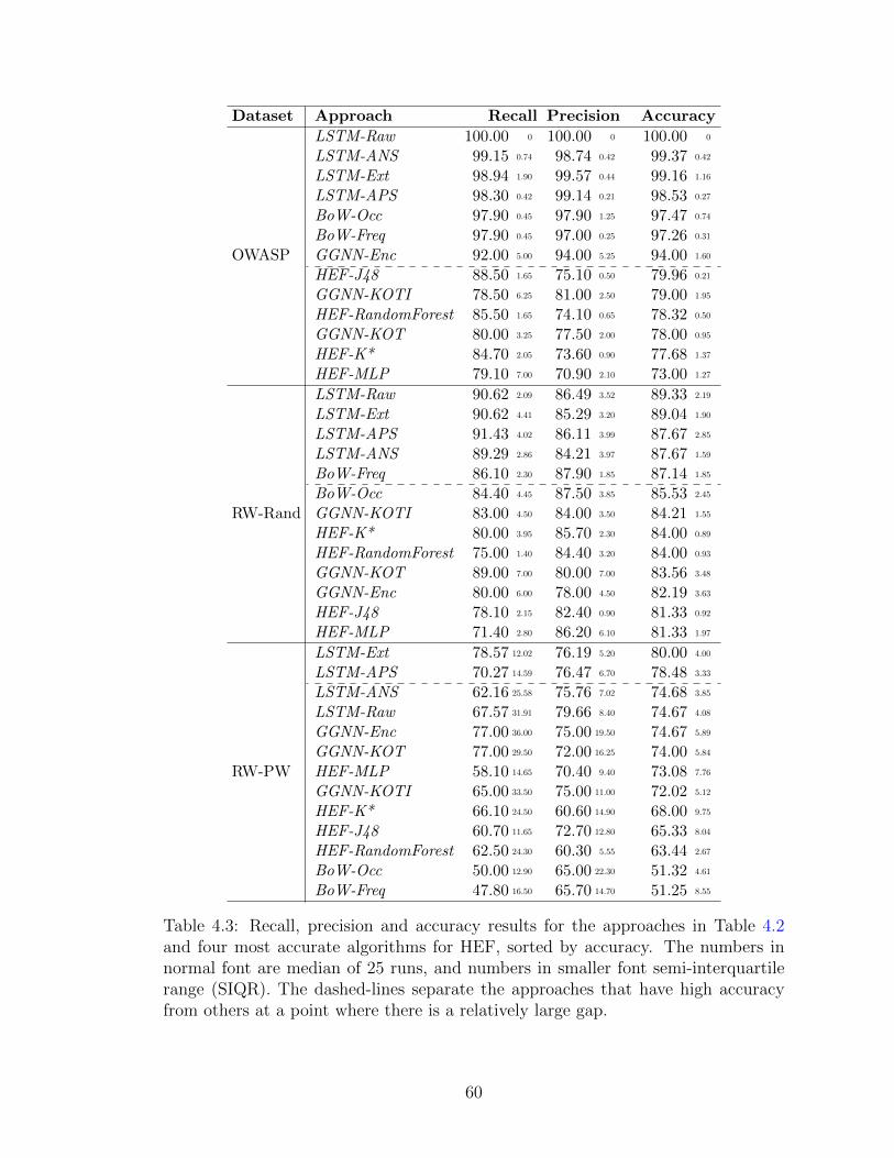
Dataset Approach Recall Precision Accuracy
OWASP
LSTM-Raw 100.00 0 100.00 0 100.00 0
LSTM-ANS 99.15 0.74 98.74 0.42 99.37 0.42
LSTM-Ext 98.94 1.90 99.57 0.44 99.16 1.16
LSTM-APS 98.30 0.42 99.14 0.21 98.53 0.27
BoW-Occ 97.90 0.45 97.90 1.25 97.47 0.74
BoW-Freq 97.90 0.45 97.00 0.25 97.26 0.31
GGNN-Enc 92.00 5.00 94.00 5.25 94.00 1.60
HEF-J48 88.50 1.65 75.10 0.50 79.96 0.21
GGNN-KOTI 78.50 6.25 81.00 2.50 79.00 1.95
HEF-RandomForest 85.50 1.65 74.10 0.65 78.32 0.50
GGNN-KOT 80.00 3.25 77.50 2.00 78.00 0.95
HEF-K* 84.70 2.05 73.60 0.90 77.68 1.37
HEF-MLP 79.10 7.00 70.90 2.10 73.00 1.27
RW-Rand
LSTM-Raw 90.62 2.09 86.49 3.52 89.33 2.19
LSTM-Ext 90.62 4.41 85.29 3.20 89.04 1.90
LSTM-APS 91.43 4.02 86.11 3.99 87.67 2.85
LSTM-ANS 89.29 2.86 84.21 3.97 87.67 1.59
BoW-Freq 86.10 2.30 87.90 1.85 87.14 1.85
BoW-Occ 84.40 4.45 87.50 3.85 85.53 2.45
GGNN-KOTI 83.00 4.50 84.00 3.50 84.21 1.55
HEF-K* 80.00 3.95 85.70 2.30 84.00 0.89
HEF-RandomForest 75.00 1.40 84.40 3.20 84.00 0.93
GGNN-KOT 89.00 7.00 80.00 7.00 83.56 3.48
GGNN-Enc 80.00 6.00 78.00 4.50 82.19 3.63
HEF-J48 78.10 2.15 82.40 0.90 81.33 0.92
HEF-MLP 71.40 2.80 86.20 6.10 81.33 1.97
RW-PW
LSTM-Ext 78.57 12.02 76.19 5.20 80.00 4.00
LSTM-APS 70.27 14.59 76.47 6.70 78.48 3.33
LSTM-ANS 62.16 25.58 75.76 7.02 74.68 3.85
LSTM-Raw 67.57 31.91 79.66 8.40 74.67 4.08
GGNN-Enc 77.00 36.00 75.00 19.50 74.67 5.89
GGNN-KOT 77.00 29.50 72.00 16.25 74.00 5.84
HEF-MLP 58.10 14.65 70.40 9.40 73.08 7.76
GGNN-KOTI 65.00 33.50 75.00 11.00 72.02 5.12
HEF-K* 66.10 24.50 60.60 14.90 68.00 9.75
HEF-J48 60.70 11.65 72.70 12.80 65.33 8.04
HEF-RandomForest 62.50 24.30 60.30 5.55 63.44 2.67
BoW-Occ 50.00 12.90 65.00 22.30 51.32 4.61
BoW-Freq 47.80 16.50 65.70 14.70 51.25 8.55
Table 4.3: Recall, precision and accuracy results for the approaches in Table 4.2and four most accurate algorithms for HEF, sorted by accuracy. The numbers innormal font are median of 25 runs, and numbers in smaller font semi-interquartilerange (SIQR). The dashed-lines separate the approaches that have high accuracyfrom others at a point where there is a relatively large gap.
60

# of epochs Training time(min)
OWASP
LSTM-Raw 170 48 23 11
LSTM-ANS 221 47 32 4
LSTM-APS 237 35 31 4
LSTM-Ext 197 79 37 20
GGNN-KOT 303 113 28 10
GGNN-KOTI 218 62 20 6
GGNN-Enc 587 182 54 17
RW-Rand
LSTM-Raw 62 1 303 1
LSTM-ANS 64 1 303 1
LSTM-APS 63 1 303 1
LSTM-Ext 50 0 304 2
GGNN-KOT 325 6 301 0
GGNN-KOTI 325 6 300 0
GGNN-Enc 326 4 300 0
RW-PW
LSTM-Raw 63 2 301 2
LSTM-ANS 65 2 301 6
LSTM-APS 65 2 302 2
LSTM-Ext 52 2 303 2
GGNN-KOT 284 54 250 47
GGNN-KOTI 215 21 194 17
GGNN-Enc 245 50 211 58
Table 4.4: Number of epochs and training times for the LSTM and GGNN ap-proaches. Median and SQIR values as in Table 4.3
the OWASP dataset, the value of the PDG nodes, i.e., the textual content of the
programs, carry useful signals to be learned during training. This also explains the
outstanding performance of the BoW and LSTM approaches, as they mainly use
this textual content in training.
For the RW-Rand dataset, two LSTM approaches achieve close to 90% accu-
racy, followed by BoW approaches at around 86%. GGNN and HEF approaches
achieve around 80% accuracy. This result suggests that the RW-Rand dataset con-
tains more relevant features the HEF approaches can take advantage of, and we
conjecture that the overall accuracy of the other three algorithms dropped because
61

of the larger programs and vocabulary in this dataset. Table 4.5 shows the number
of the words and length of samples for the LSTM approaches (the normal font is
the maximum while the smaller font is the mean). As expected, the dictionary gets
smaller while the samples get larger as we apply more data preparation. For GGNN,
the number of nodes is 24 on average and 82 at most, the number of edges is 47 on
average and 174 at most in the OWASP dataset. The real-world dataset has 1880
average to 16 479 maximum nodes, and 6411 average to 146 444 maximum edges.
The real-world programs are significantly larger than the OWASP programs, both
in dictionary sizes and sample lengths.
For the RW-PW dataset, all the accuracy results except LSTM-Ext are below
80%. Recall that this split was created for the second application scenario where the
training is performed using one set of programs, and testing is done using others.
We observe the neural networks (i.e., LSTM and GGNN) still produce reasonable
results, while the results of HEF and BoW dropped significantly. This suggests
that neither the hand-engineered features nor the textual content of the programs
are adequate for the second application scenario, without learning any structural
information from the programs.
Next, Both HEF and BoW approaches are very efficient. All their variations
completed training in less than a minute for all datasets, while the LSTM and GGNN
approaches run for hours for the RW-Rand and RW-PW datasets (Table 4.4). This
is mainly due to the large number of parameters being optimized in the LSTM and
GGNN.
Lastly, note that the results on the OWASP dataset (Table 4.3) are directly
62

comparable with the results we achieved in the case study presented in the preivous
chapter [71], which report 85% and 90% accuracy for program slice and control-flow
graph representations, respectively. In this paper, we only experimented with pro-
gram slices as they are a more precise summarization of the programs. With the
same dataset, our LSTM-Ext approach, which does not learn from any program-
specific tokens, achieves 99.57% accuracy. Therefore, we conjecture these improve-
ments are due to the better and more precise data preparation routines we perform.
4.4.2 RQ2: Effect of Data Preparation
Dictionary size Sample lengthApproach OWASP real-world OWASP real-worldLSTM-Raw 333 13 237 735 224 156 393 18524
LSTM-ANS 284 9724 706 212 149 886 18104
LSTM-APS 284 9666 706 212 150 755 18378
LSTM-Ext 251 4730 925 277 190 950 23031
Table 4.5: Dataset stats for the LSTM approaches. For the sample length, numbersin the normal font are the maximum and in the smaller font are the mean.
We now analyze the effect of different data preparation techniques for the
machine learning approaches. Recall the goal of data preparation is to provide
the most effective use of information that is available in the program context. We
found that LSTM-Ext produced the overall best accuracy results across the three
datasets. The different node representations of GGNN present tradeoffs, while the
BoW variations produced similar results.
Four code transformation routines were introduced for LSTM. LSTM-Raw
achieves 100% accuracy on the OWASP dataset. This is because LSTM-Raw per-
63

forms only basic data cleansing and tokenization, with no abstraction for the vari-
able, method, and class identifiers. Many programs in the OWASP benchmark
have variables named “safe,” “unsafe,” “tainted,” etc., giving away the answer to
the classification task and causing memorizing the program-specific and concrete
information from this dataset. Therefore, LSTM-Raw can be suitable for the first
application scenario in which learning program-specific and concrete things can help
learning. On the other hand, the RW-PW dataset benefits from more transformation
routines that perform abstraction and word extraction. LSTM-Ext outperformed
LSTM-Raw by 5.33% in accuracy for the RW-PW dataset.
We presented three node representation techniques for GGNN. For the OWASP
dataset, we observe a significant improvement in accuracy from 78% with GGNN-
KOT to 94% with GGNN-Enc. This suggests that very basic structural informa-
tion from the OWASP programs (i.e., the kind, operation, and type information
included in GGNN-KOT ) carries limited signal about true and false positives, while
the textual information included in GGNN-Enc carries more signal, leading to a
large improvement. This trend, however, is not preserved on the real-world datasets.
All GGNN variations, i.e., GGNN-KOT, GGNN-KOTI, and GGNN-Enc, performed
similarly with 83.56%, 84.21%, and 82.19% accuracy, respectively, on the RW-Rand,
and 74%, 72%, and 74.67% accuracy on the RW-PW datasets. Overall, we think
the GGNN trends are not clear partly because of the nature of data such as sample
lengths, dictionary, and dataset sizes (Tables 4.1 and 4.5). Moreover, the infor-
mation encoded in the GGNN-KOT and GGNN-KOTI approaches is very limited,
whereas the information encoded in GGNN-Enc might be too much (taking the av-
64
erage over the embeddings of all tokens that appear in the statement), making the
signals harder to learn.
BoW-Occ and BoW-Freq had similar accuracy in general. The largest differ-
ence is 85.53% and 87.14% accuracy for BoW-Occ and BoW-Freq, respectively, on
the RW-Rand dataset. This result suggests that checking the presence of a word is
almost as useful as counting its occurrences.
4.4.3 RQ3: Variability Analysis
In this section, we analyze the variance in the recall, precision, and accuracy
results using the semi-interquartile range (SIQR) value given in the smaller font in
Table 4.3.
Note that, unlike other algorithms, J48 and K* deterministically produce the
same models when trained on the same training set. The variance observed for J48
and K* is only due to the different splits of the same dataset.
On the OWASP dataset, all approaches have little variance, except for a 7%
SIQR for the recall value of HEF-MLP.
On the RW-Rand dataset, SIQR values are relatively higher for all approaches
but still under 4% for many of the high performing approaches. The BoW-Freq
approach has the minimum variance for recall, precision, and accuracy. The LSTM-
ANS and LSTM-Ext follow this minimum variance result. Last, the HEF-based
approaches lead to the highest variance overall.
On the RW-PW dataset, the variance is even bigger. For recall, in particular,
65

we observe SIQR values around 30% with some of the HEF, LSTM, and GGNN
approaches. The best performing two LSTM approaches, LSTM-Ext and LSTM-
APS, have less than 4% difference between quartiles in accuracy. We conjecture this
is because the accuracy value directly relates to the loss function being optimized
(minimized), while recall and precision are indirectly related. Lastly, applying more
data preparation for LSTM leads to a smaller variance for all the three metrics for
the PW-RW dataset.
4.4.4 RQ4: Further Interpreting the Results
To draw more insights on the above results, we further analyze four represen-
tative variations, one in each family of approaches. We chose HEF-J48, BoW-Freq,
LSTM-Ext, and GGNN-KOT because these instances generally produce the best
results in their family. Figure 4.2 shows Venn diagrams that illustrate the distri-
bution of the correctly classified reports, for these approaches with their overlaps
(intersections) and differences (as the mean for 5 models). For example, in Figure
4.2-A, the value 294 in the region covered by all four colors means these reports
were correctly classified by all four approaches, while the value 1.8 in the blue only
region mean these reports were correctly classified only by LSTM.
The RW-Rand results in Figure 4.2-B show that 43 reports were correctly
classified by all four approaches, meaning these reports have symptoms that are
detectable by all approaches. On the other hand, 30.6 (41%) of the reports were
misclassified by at least one approach.
66

A - The OWASP benchmark dataset:
B - RW-Rand dataset:
C - RW-PW dataset:
Figure 4.2: Venn diagrams of the number of correctly classified examples for HEF-J48, BoW-Freq, LSTM-Ext, and GGNN-KOT approaches, average for 5 modelstrained.
67
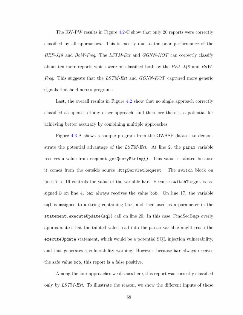
The RW-PW results in Figure 4.2-C show that only 20 reports were correctly
classified by all approaches. This is mostly due to the poor performance of the
HEF-J48 and BoW-Freq. The LSTM-Ext and GGNN-KOT can correctly classify
about ten more reports which were misclassified both by the HEF-J48 and BoW-
Freq. This suggests that the LSTM-Ext and GGNN-KOT captured more generic
signals that hold across programs.
Last, the overall results in Figure 4.2 show that no single approach correctly
classified a superset of any other approach, and therefore there is a potential for
achieving better accuracy by combining multiple approaches.
Figure 4.3-A shows a sample program from the OWASP dataset to demon-
strate the potential advantage of the LSTM-Ext. At line 2, the param variable
receives a value from request.getQueryString(). This value is tainted because
it comes from the outside source HttpServletRequest. The switch block on
lines 7 to 16 controls the value of the variable bar. Because switchTarget is as-
signed B on line 4, bar always receives the value bob. On line 17, the variable
sql is assigned to a string containing bar, and then used as a parameter in the
statement.executeUpdate(sql) call on line 20. In this case, FindSecBugs overly
approximates that the tainted value read into the param variable might reach the
executeUpdate statement, which would be a potential SQL injection vulnerability,
and thus generates a vulnerability warning. However, because bar always receives
the safe value bob, this report is a false positive.
Among the four approaches we discuss here, this report was correctly classified
only by LSTM-Ext. To illustrate the reason, we show the different inputs of these
68

1 public void doPost(HttpServletRequest request...){
2 String param = request.getQueryString();
3 String sql, bar, guess = "ABC";
4 char switchTarget = guess.charAt(1); // ’B’
5 // Assigns param to bar on conditions ’A’ or ’C’
6 switch (switchTarget) {
7 case ’A’:
8 bar = param; break;
9 case ’B’: // always holds
10 bar = "bob"; break;
11 case ’C’:
12 bar = param; break;
13 default:
14 bar = "bob’s your uncle"; break;
15 }
16 sql = "UPDATE USERS SET PASSWORD=’" + bar + "’ WHERE USERNAME=’foo’";
17 try {
18 java.sql.Statement statement = DatabaseHelper.getSqlStatement();
19 int count = statement.executeUpdate(sql);
20 } catch (java.sql.SQLException e) {
21 throw new ServletException(e);
22 }
23 }
(A)
1 org owasp benchmark UNK UNK do Post ( Http Servlet Request Http
Servlet Response ) :
2 String VAR 6 = p 1 request get Query String ( ) :
3 C VAR 10 = STR 1 char At ( 1 ) :
4 switch VAR 10 : String Builder VAR 14 = new String Builder :
5 String Builder VAR 18 = VAR 14 append ( STR 0 ) :
6 String Builder VAR 20 = VAR 18 append ( VAR 13 ) :
7 String Builder VAR 23 = VAR 20 append ( STR 3) :
8 String VAR 25 = VAR 23 to String ( ) :
9 java sql Statement VAR 27 = get Sql Statement ( ) :
10 I VAR 29 = VAR 27 execute Update ( VAR 25 ) :
11 PHI VAR 13 = VAR 6 STR 4 VAR 6 STR 2
(B)
Figure 4.3: An example program (simplified) from the OWASP benchmark that wascorrectly classified only by LSTM-Ext (A) and the sequential representation usedfor LSTM-Ext (B)
approaches. Figure 4.3-B shows the sequential representation used by LSTM-Ext.
69

HEF-J48 used the following feature vector:
[[[rule namerule namerule name : SQL INJECTION,
sink linesink linesink line : 19, sink identifiersink identifiersink identifier : Statement.executeUpdate,
source linesource linesource line : 2, source identifiersource identifiersource identifier : request.getQueryString,
functionsfunctionsfunctions : 4,
witness lengthwitness lengthwitness length : 2,
number bugsnumber bugsnumber bugs : 1,
conditionsconditionsconditions : 1, severityseverityseverity : 5, confidenceconfidenceconfidence : High,
timetimetime : 2,
classes involvedclasses involvedclasses involved : 1]]]
Notice that this feature vector does not include any information about the
string variable guess, the switch block, or overall logic that exists in the program.
Instead, it relies on correlations that might exist for the features above. For this
example, such correlations weight more for the true positive decision, thus lead to
misclassification.
On the other hand, the LSTM-Ext representation includes the program infor-
mation. For example, VAR 6 gets assigned to the return value of the request.get
QueryString method and VAR 10 is defined as STR 1 . char At (1). Note that
STR 1 refers to the first string that appears in this program, i.e., ‘‘ABC’’). We see
the tokens switch VAR 10 at line 5 corresponding to the switch statement. Then,
we see string and SQL operations through lines 7 to 12, followed by a PHI instruction
at line 13. This sequential representation helps LSTM-Ext to correctly classify the
example as a false positive.
70
Last, BoW-Freq misclassified this example using the tokens in Figure 4.3-B
without their order. This suggests that the overall correlation of the tokens that
appear in this slice does not favor the false positive class. We argue that the correct
classification by LSTM-Ext was not due to the presence of certain tokens, but rather
due to the sequential structure.
4.4.5 Threats To Validity
There are several threats to the validity of our study. First, the benchmarks
may not be representative. Like we mentioned earlier, the OWASP benchmark is
synthetic. Therefore, we collected the first real-world benchmark for classifying
static analysis results, consisting of 14 programs to increase the generalizability
of our results. In addition, our real-world benchmark consists of 400 data points,
which may not be large enough to train neural networks with high confidence. We
repeated the experiments using different random seeds and data splittings to ana-
lyze the variability that might be caused by having limited data. Second, we ran
our experiments on a virtual machine, which may affect the training times. How-
ever, since these models would be trained offline and very rarely, we are primarily
interested in the effectiveness of the approaches in this study.
4.5 Attributions and Acknowledgments
The study presented in this chapter is supported by the Department of Home-
land Security under the grant #D15PC00169 and published in the proceedings
71

of 2019 12th IEEE Conference on Software Testing, Validation and Verification
(ICST’19) [18]. All development and experimentation tasks are carried out by me,
Ugur Koc, with the guidance and supervision of other collaborators.
72

Chapter 5: Auto-tuning Configurable Program Verification Tools
Many static program verification tools can be customized by setting runtime
configuration options. For example, CBMC [99], a popular verification tool for
C/C++ programs, has 98 configuration options, such as --unwind which specifies
the number of times to unwind loops when computing the model of the program.
Most of these options present tradeoffs between performance, precision, and sound-
ness. Although these options allow users to customize the tools for their own needs,
choosing the best options for a specific task is challenging, requiring domain exper-
tise and extensive experimentation [19]. In addition, the effectiveness of an setting
an option (or a combination of options) can depend on the features present in the
target program [24, 100], making it difficult to find a single configuration that pro-
duces desirable results (e.g., fast and precise) for differing programs. In practice,
users, especially a non-experts, often run a static bug detector on target programs
with a provided “default” configuration to see if it produces desirable outputs. If
not, these users often do not know how to effectively modify the analysis options to
produce better results. We believe this challenge has prevented many verification
tools from being used to their full potential.
Recent studies have shown that configuration options indeed present tradeoffs
73

[19], especially when different program features are present [20, 21, 22]. Various
techniques have been proposed that selectively apply a configuration option to cer-
tain programs or parts of a program (i.e., adaptive analysis), using heuristics defined
manually or learned with machine learning techniques [20, 23, 21, 24, 22, 25]. Al-
though a promising research direction, these techniques are currently focused on
tuning limited kinds of analysis options (e.g., context-sensitivity). In addition, ma-
chine learning techniques have recently been used to improve the usability of static
analysis tools. The applications include classifying, ranking, or prioritizing analy-
sis results (like the learning approach we introduced and evaluated in Chapters 3
and 4) [9, 10, 26, 27, 7, 28, 29], and ranking program verification tools based on
their likelihood of completing a given task [30, 31]. However, the configurability of
static analysis tools, verification tools specifically, has not been considered in these
applications. We believe that automatic configuration selection will make pro-
gram verification tools more usable and enable their wide adoption in the software
engineering practice.
In this chapter, we present auto-tune to automatically configure program
verification tools for given target programs. We aim to develop a generalizable ap-
proach that can be used for various tools that are implemented in and targeted
at different programming languages. We also aim to develop an efficient approach
that can effectively search for desirable configurations in large spaces of configura-
tions. To achieve these goals, our approach leverages two main ideas. First, we use
prediction models using supervised machine learning as both fitness functions and
incorrect result filters. Our prediction models are trained on language-independent
74

features in target programs and configuration options of the subject verification
tools. Second, we use a meta-heuristic search algorithm that probabilistically scans
the configuration spaces of verification tools using the aforementioned prediction
models.
Overall, auto-tune works as follows: we first train two prediction models to
be used in the meta-heuristic search algorithm using a ground-truth dataset that
consists of correct, incorrect, and inconclusive1 program analysis runs. The first
model, the fitness function, is trained on the entire dataset; the second model, the
incorrect result filter (or, for short, filter), is trained only on the conclusive part of
the dataset –i.e., we exclude the inconclusive analysis runs. Our search algorithm
starts with a default configuration of the tool if available; otherwise, it starts with a
random configuration. The algorithm then systematically, but non-deterministically,
alters this configuration to generate a new configuration. Throughout the search,
the fitness function is used to decide whether a configuration is good enough to
accept as the current candidate solution, and the filter is used to decide whether
to run the tool with this configuration or not. The algorithm continues to scan the
search space by generating new configurations until it locates one that meets the
thresholds in the fitness and filter functions and that leads to a conclusive result
when run.
auto-tune is a meta-reasoning approach [32, 33] because it aims to reason
about how verification tools should reason about a given verification task. In this
1An inconclusive analysis run means the tool fails to come to a judgement due to a timeout,crash, or a similar reason.
75
setting, the reasoning of a given verification tool is controlled by configuration op-
tions that enable/disable certain simplifications or assumptions throughout the anal-
ysis tasks. The ultimate goal of meta-reasoning is to identify a reasoning strategy,
i.e., a configuration, that is likely to lead to the desired verification result.
We applied auto-tune to four popular program verification tools. CBMC and
Symbiotic [34, 35] verify C/C++ programs, while JBMC [36] and JayHorn [37] verify
Java programs. We generated program analysis datasets with the ground truths
from the SV-COMP2, an annual competition of software verification that includes
a large set of both Java and C programs. We used our datasets, which contain
between 55K and 300K data points, to train prediction models for each tool.
To evaluate the effectiveness of auto-tune, we consider two use cases. First,
to simulate the scenario in which a non-expert uses a tool without a reliable de-
fault configuration, we start auto-tune with a random configuration. Our experi-
ments suggest that auto-tune could produce results comparable to configurations
manually and painstakingly selected by program analysis experts (referred to as
comp-default3 in the remainder of this chapter). Second, to simulate the scenario
in which a tool comes with a reliable default configuration, or is used by an expert,
we start auto-tune with the comp-default configuration. Our results suggest that,
with regard to the competition’s scoring system, auto-tune could improve the SV-
COMP performance for three out of four program verification tools we studied:
Symbiotic, JayHorn, and JBMC . For CBMC , auto-tune also increased the num-
2https://sv-comp.sosy-lab.org/20193These are the configurations the tools used when participating the competition.
76

ber of correct analysis runs significantly, but it did not improve the competition
score due to the large penalty for incorrect results. We also studied the effects of
different choices in our algorithm, including two supervised machine learning ap-
proaches (i.e., classification and regression) and three strategies for creating a new
configuration in the search.
In summary, the contributions of our work are:
• A novel meta-heuristic search approach to automatically configure program
verification tools, using machine learning models both as a fitness function
and as a false result filter
• Successful applications of the approach to four state-of-the-art verification
tools for C and Java (Section 5.4).
• The collection and analysis of ground-truth datasets, showing the distribution
of results across different analysis configurations (Section 5.4).
• Empirical evaluations of different use-case scenarios that demonstrate the ef-
fectiveness of auto-tune and an in-depth study of the choices in the algo-
rithm (Section 5.5).
We have made the implementation, datasets and evaluation results publicly
available: https://bitbucket.org/ugur_koc/auto-tune
77

1 extern void __VERIFIER_error() __attribute__ ((__noreturn__));
2 void __VERIFIER_assert(int cond) {
3 if(!(cond)) { ERROR: __VERIFIER_error(); }
4 }
5
6 #define N 100000
7
8 int main( ) {
9 int min = 0, i = 0, a[N];
10 while ( i < N ) {
11 if ( a[i] < min )
12 min = a[i];
13 i++;
14 }
15 for (int x = 0 ; x < N ; x++ ) {
16 __VERIFIER_assert( a[x] >= min );
17 }
18 return 0;
19 }
A - Program P1
1 extern void __VERIFIER_error() __attribute__ ((__noreturn__));
2 void __VERIFIER_assert(int cond) {
3 if(!(cond)) { ERROR: __VERIFIER_error(); }
4 }
5
6 #define N 100000
7
8 int main( ) {
9 int src[N], dst[N], i = 0;
10 while ( src[i] != 0 ){
11 dst[i] = src[i++];
12 }
13 for (int x = 0 ; x < i ; x++ ) {
14 __VERIFIER_assert( dst[x] == src[x] );
15 }
16 return 0;
17 }
B - Program P2
Figure 5.1: Code examples from the SV-COMP 2018.
78

5.1 Motivating Examples
We now demonstrate the challenges involved in configuring verification tools
using the two motivating examples in Figure 5.1. These two example programs are
extracted from SV-COMP 2018 [101]. Both popular C verification tools we studied,
CBMC and Symbiotic, produce inconclusive analysis results (i.e., timeout in 15 min-
utes or crash with out of memory error) using their developer-tuned comp-default
configurations on these programs. This leaves the tool users uncertain about whether
they can successfully analyze these programs with other configurations.
Figure 5.1-A presents a safe program, P1. Its main functionality is to find
the minimum value in the integer array a (lines 10-14). Line 16 uses an assertion
to check if all the elements are greater than or equal to the computed minimum
value. If the assertion fails, it triggers the ERROR on line 3. While, in fact, the ERROR
cannot be reached in any execution of this program, CBMC ’s comp-default led
to inconclusive results. To understand the difficulty of successfully analyzing this
program, we manually investigated 402 configurations of CBMC. Only 48 (12%) of
them lead to the correct analysis result, while others were inconclusive. We identified
that --depth=100, which limits the number of program steps, is the only option
value that is common in successful configurations and different from its value (no
depth limit) in comp-default. Using this option value is critical when analyzing P1
because it improves the scalability of CBMC so that it finishes within the time limit.
We made similar observations on the configurations of Symbiotic. Investigating the
configurations that led to the correct result, 81 out of 222, we found that it is critical
79

to turn the --explicit-symbolic4 option on for Symbiotic to scale on P1 rather
than using comp-default which turns it off. This example demonstrates that some
options may be important for improving the performance of certain verification
tools on certain programs and that altering them from the default configurations
may yield better analysis results.
Figure 5.1-B shows an unsafe program, P2, with an array-out-of-bounds error.
At lines 10-11, the program copies elements from src array to dest array in a loop
until it reaches 0 in src. At lines 13-14, the assertion checks if src and dest have
the same elements up to index i. The problem with this program is that if src does
not contain 0, the array accesses at line 10 will exceed the bounds of the arrays. Re-
call that Symbiotic’s comp-default also led to an inconclusive result on P2. From a
manual investigation of P1, we know that turning on option --explicit-symbolic
may be critical to the performance of the tool. However, doing this leads to incorrect
results on P2 due to unsoundness, because the random values used for initialization
may actually contain 0. Out of the 137 Symbiotic configurations we manually in-
vestigated for P2, only 3 of them led to the correct analysis result, while 123 were
inconclusive, and 12 were incorrect. In the 12 configurations leading to the incorrect
result, --explicit-symbolic was always on.
The above motivating examples show that there may not exist a single config-
uration under which a tool performs well across all programs, because the options
interact differently with programs depending on the programs’ features. However,
4Setting --explicit-symbolic:on in Symbiotic results in initializing parts of memory withnon-deterministic values. Otherwise, evaluation is done with symbolic values which leads trackingmore executions paths (costly).
80

such manual investigation is costly and requires domain expertise, demonstrating
the need for auto-tune, whose goal is to automatically locate tool configurations
that are likely to produce desired analysis results for a given program.
5.2 Our Auto-tuning Approach
Figure 5.2: Workflow of our auto-tuning approach.
One way to perform auto-tuning is to train classifiers to predict the appropriate
settings for all configuration options (a configuration consisting of many analysis
options), given a target program to analyze. This can be achieved with multi-target
classification [102] by treating each configuration option as a label. However, as
our motivating examples show, only a few options may be strongly associated with
certain program features. This means that in order to achieve high accuracy in
a multi-target learning model, the ground-truth dataset should have many data
points for these options while the replications of the other options represent noise.
Without knowing in advance which analysis options are important, prohibitively
81

large datasets would be required in order to contain the necessary replications of each
configuration option. Alternatively, the amount of data needed sharply decreases if
one is able to frame the problem as a single target problem, instead of a multi-target
problem. Our idea for auto-tune is to formulate the problem as a search problem
that uses models trained from single target classification/regression.
Figure 5.2 shows the workflow of auto-tune. The key component is a meta-
heuristic configuration search that navigates through a tool’s configuration space
and makes predictions about candidate configurations using machine learning mod-
els trained offline. To use auto-tune, a user provides a target program and an
optional initial configuration. auto-tune runs the tool with the initial configura-
tion if provided. If the initial configuration leads to an inconclusive result or if the
user does not provide an initial configuration (e.g., a good default configuration
of a tool is not available), auto-tune explores the configuration space to locate a
configuration likely to produce conclusive and correct analysis results for the tar-
get program (using thresholds and prediction models). The located configuration
is then used to run the verification tool. The search algorithm is iteratively ap-
plied until a conclusive analysis result is produced, or the search terminates after
being unable to find a conclusive result. This workflow applies to automatically
configuring many configurable program verification tools.
82

Algorithm 2 Meta-heuristic configuration search algorithm
1: function ConfigSearch(CS= 〈O,D〉, P , M , F , θ)2: T ← 1;Ts ← 10−5;R← 10−4 . hyper parameters3: analysisResult← −999 . analysis exit code4: V ← getProgramRepresentation(P )5: c∗ ← c← getInitialConfig(CS)6: Ec∗ ← Ec ← query(M, 〈V ++ c〉) . cost for 〈V ++ c〉7: while Ts < T ∧¬isComplete(analysisResult) do8: repeat9: c′ ← generateNeighboringConfig(CS, c)
10: Ec′ ← query(M, 〈V ++ c′〉)11: ∆E ← Ec′ − Ec12: T ← T − (T ×R)13: until ∆E < 0 ∨ rand(0, 1) < e−k∆E/T
14: c, Ec ← c′, Ec′15: if Ec < Ec∗ then16: c∗, Ec∗ ← c, Ec . best config so far17: Sc←query(F, 〈V++c〉) . incorrectness score for 〈V++c〉18: if Sc≤θ then
19: analysisResult← runSA(P, c)
20: return 〈analysisResult, c∗〉
5.2.1 Meta-heuristic Configuration Search
We now present our meta-heuristic configuration search algorithm, which ef-
fectively explores and predicts configurations from a subset of a tool’s configurations.
Our algorithm is inspired by simulated annealing [103, 104, 105]. Simulated
annealing is a meta-heuristic search algorithm that mimics the metallurgical process
of annealing. It probabilistically scans the search space to approximate the globally
optimal solution). Generally, simulated annealing starts from an initial state and
iteratively searches for a good solution by applying alterations to the current state.
This generates a new candidate state (i.e., neighboring state). If the generated
83

neighboring state is better than the current state, it is “accepted” as the current
state for the next search iteration. Otherwise, to avoid getting stuck in local optima,
“inferior” neighboring states are probabilistically accepted. There are three control
parameters in simulated annealing: the initial temperature T0, the cooling rate R by
which the temperature T is reduced every iteration, and the stopping temperature
Ts. At any given iteration t, the temperature Tt determines the probability that an
inferior neighbor state is accepted as the new current state. This has the effect of
reducing the probability that inferior neighboring states are accepted as the search
progresses; i.e., inferior neighboring states are more likely to be accepted at early
iterations. The search ends either when a good solution is found, or when the
temperature reaches Ts.
Algorithm 2 shows our meta-heuristic configuration search. The inputs to this
algorithm are:
1. the tool’s configuration space CS = 〈O,D〉 where O is the set of configuration
options and D is their domains,
2. the target program P ,
3. the fitness function model M ,
4. the filter model F , and
5. the threshold value θ for the incorrectness score computed by the filter.
Lines 2-6 perform the initializations. First, we initialize the hyper-parameters
as follows: T = 1, Ts = 10−5, and R = 10−4 (empirically determined). The variable
84

analysisResult is set to −999, referring to an inconclusive analysis result. Line 4
extracts the program features of P and assigns them to V . At line 5, the current
configuration (c) and the best configuration (c∗) are both initialized with either a
default configuration provided by the user or a randomly generated configuration.
At line 6, M is used to compute Ec, which is the predicted cost of this configuration
running on a program with features V . Depending on whether M is configured as a
classification or regression model (see Section 5.2.2), this cost can be a continuous
score (regression) or the probability that c will produce either an inconclusive or
incorrect result).
Lines 7 to 19 are the search iterations. Line 7 has two guards: Ts < T , to
check that the temperature has not decreased below the stopping temperature, and
isComplete(analysisResult), which stops the search when a conclusive result has
been produced (since our goal is only to find a “good” rather than “the optimal”
solution). The inner loop at lines 8-13 generates the neighboring configuration c′
(line 9), predicts its cost using M (line 10), and repeats until one of the acceptance
conditions on line 13 is met. There are two reasons a c′ can be accepted as the cur-
rent configuration c: either it is better than c (∆E < 0), or because the probabilistic
condition indicating whether to accept an inferior state, rand(0, 1) < e−k∆E/T , holds
(line 13). The current solution c and current cost Ec are then updated, according
to the generated configuration at line 14. If the fitness model predicts the current
configuration is the best so far (Ec < Ec∗), C∗ and Ec∗ are also updated accordingly
(lines 15-16). When a new configuration is determined to be the best, we want to
run the analysis tool and update analysisResult accordingly. However, running the
85

analysis tool is an expensive operation. We thus use a second prediction model F
on line 17, the filter, to predict an “incorrectness score;” in other words, the likeli-
hood that running the tool with the configuration will return an incorrect analysis
result. We predict this score Sc, and only run the analysis tool if Sc is less than
the parameter θ (lines 18-19). If the analysis produces conclusive results, the search
ends, and we return the analysis results (line 20). Otherwise, the search continues.
To summarize, our search algorithm adapts simulated annealing with three
key enhancements specific to our application:
1. The algorithm does not require finding the optimal solution but rather, a good
solution, which is implemented through the additional stopping condition,
isComplete(analysisResult).
2. The cost estimated by the fitness function model, Ec, is not just the cost of
a configuration c, but the cost of the configuration and program pair 〈V ++ c〉
3. The filter model and the control mechanism that uses this model to decide
whether to run the analysis tool or not (lines 17-19).
5.2.2 Learning the Fitness Function and Filter
Data Structure. A data point in our dataset is precisely what is used to query the
fitness function in the search process; i.e.,
V ++ c = X
where V is the program feature vector, ++ is the concatenation operator, c is the
configuration, and X is the analysis result (i.e., correct, incorrect, and inconclusive).
86

This way, when predicting an analysis result for a new program and configuration
pair, the machine learning algorithms will not just use program features or config-
uration options, but also their interactions.
Feature Extraction. Recall that one of our goals is to be able to apply our ap-
proach to tools targeted at analyzing programs in different languages. Therefore,
we extract generic program features that are available in most (if not all) program-
ming languages. We use a simple bag of words technique that has been used in the
analysis report classification study (presented in Chapter 4) [18]. We only count
the number of each kind of intermediate level instructions in three-address code and
loops. In particular, we use 56 LLVM IR [106] instructions for C and 33 WALA
IR [64] instructions for Java.
Prediction Models. To navigate in the search space, we need a way to measure the
cost/fitness of each candidate solution. We achieve this through a fitness function.
The fitness function should output continuous numerical cost values for candidates.
In this problem, we do not know what the exact costs of configurations are; therefore,
we approximate this cost by using a prediction model as a fitness function. We
achieve this in two alternative ways. One way is to train classifiers and use them to
compute the probability that a data point (V ++ c) results in either an inconclusive
or incorrect analysis result. This probability is used as the cost/fitness of the data
point.
Alternatively, we can map classes of analysis results to certain numeric values
87

and train regression models. Now, the regression models’ output is used as the cost.
In this case, since our search is designed as a minimization problem, i.e., aiming
to reduce the cost, the desired analysis results should be mapped to values smaller
than the values of undesired (i.e., incorrect and inconclusive) analysis results. One
advantage of the regression approach is customizability; i.e., the distance between
the correct and incorrect classes can be adjusted for different scenarios. In certain
application domains, missing a buggy program (i.e., false negative, FN) is not ac-
ceptable. To account for that, we can assign a very high-cost value to FN class
while a relatively low-cost value to FP class. This way, our approach can tolerate
FP results, but the goal is to avoid missing any buggy/defective in programs. In
other application domains, FN results might be acceptable, while wasting develop-
ers’ time and other resources on FP results are not. Accordingly, the cost value for
FP can be set high, and the cost value for FN relatively low.
We explore both of these approaches, i.e., classification and regression, in our
study. We provide and discuss the cost values we used in our evaluations with
regression models in Section 5.5.1.
Once we have candidate configurations, our next goal is to reduce the likelihood
of selecting a final configuration that produces an incorrect result. We thus utilize
a second prediction model–the incorrect result filter–that is used in the search to
compute the likelihood of a data point (V ++c) corresponding to an incorrect analysis
result. We call the output of this filter an incorrectness score. We train the filter in
the same way as the fitness function, using classification or regression. In fact, the
only difference between the fitness function and the filter is the dataset they trained
88

on. The fitness function is trained on the entire dataset, so, ideally, it can learn
the relations between the data and analysis results, including the inconclusive ones.
The filter, however, is trained on the conclusive analysis runs only in order to make
the filter more specialized for learning program features, configuration options, and
their potential interactions that might lead to incorrect analysis results.
To obtain the ground-truth datasets for a given verification tool, we system-
atically select sample configurations from its configuration space and run it with
each selected configuration on a set of benchmark programs with known correctness
properties (i.e., unsafe or safe). After generating the labeled dataset, we train two
models to be used in the configuration search, as described in Section 5.2.1.
5.2.3 Neighboring Configuration Generation
The neighbor generation strategy of any search algorithm is an essential com-
ponent that can significantly affect performance. A good neighbor generation strat-
egy should select good candidates to direct the search for scanning the entire space
in a cost-effective manner. One common way to generate neighboring states is to
alter the current state randomly.
We have three different neighbor generation strategies. First, as the baseline,
we generate a neighboring configuration by altering the current configuration at a
maximum of three random points with no restrictions. These alterations take place
randomly within the domain of each option, which is defined manually. We call this
strategy the base strategy.
89

In order to come up with more sophisticated strategies, we performed a main
effect screening study [107] on the ground-truth datasets. We observed that there
are configuration option values that have statistically significant effects on the num-
ber of correct, incorrect, and/or inconclusive analysis results. We implement two
alternative neighbor generation strategies that make use of these findings.
The second strategy is the greedy strategy. For this strategy, when the current
configuration is altered to produce the neighboring configuration, we forbid any
values of an option oi,j (referring to the jth value of option i) that increases the
number of incorrect results by significantly more than it increases the number of
correct results. However, if an option value is contributing to both the correct and
incorrect classes equally, we do not forbid it. We expect the fitness function to learn
the interactions between such option settings and program features and favor the
setting that is likely to lead to the correct analysis result for a given program.
The third strategy is the conservative strategy. In this strategy, any oi,j that
increases the number of incorrect results is forbidden, regardless of whether it also
increased the number of correct results.
To identify the forbidden option values for the greedy and conservative strate-
gies, we performed main effect screening studies on the ground-truth datasets using
JMP [108]. Any option value that increases incorrect results and has a statisti-
cally significant effect p < 0.05 according to the screening study is forbidden during
neighbor generation if the appropriate rule applies.
90

5.3 Implementation
We implemented the proposed approach in 600 lines of Java code5. Specifically,
we used the random forest algorithm6 for classification [110] and the REP (stands
for Reduced-Error Pruning) tree algorithm7 for regression [111] (both with default
parameters). In this implementation, supervised training of the predictive models
and search are automated.
It takes as input:
1. the training and testing dataset files;
2. an executable script to run the verification tool;
3. the choice of starting point (default or random config);
4. choice of neighbor generation strategy (base, greedy, or conservative);
5. choice of learning model (regression or classification); and
6. threshold value (there are other optional inputs we do not list here, see --help
option of the tool).
First note, if the starting point is chosen as the default config (the default
config file must be present), the search will start only if the default config fails to
return a conclusive analysis result. Second note, the threshold values are at different
scale for classification and regression. For classification, it should be between 0-1,
5Weka Dev 3.9.3 [109] is the only framework that we have as a dependency for the machinelearning algorithms.
6Implementation: weka.classifiers.trees.RandomForest7Implementation: weka.classifiers.trees.REPTree
91

where 0 will lead to very conservative runs that will filter any configuration that
is not guaranteed to complete with a correct result, while 1 means no threshold.
For regression, this value will depend on the numeric value mappings the classes
have. For example, if the correct classes are mapped to 0, and incorrect classes are
mapped to 100, a threshold value of 10 will cause filtering any configurations that
lead to a falseness score grader than 10.
5.4 Datasets
In this section, we describe the subject analysis tools we used in our evaluation,
benchmark programs, and the ground-truth dataset we created for each subject tool.
5.4.1 Subject Tools
Target # of Config Sample DatasetTool lang options space size size sizeCBMC 5.11 C 21 2.9 × 10⁹ 295 295 000Symbiotic 6.1.0 C 16 9.8 × 10⁵ 82 54 940JayHorn 0.6-a Java 12 7.5 × 10⁶ 256 94 208JBMC 5.10 Java 27 7.2 × 10¹⁰ 200 73 600
Table 5.1: Subject verification tools.
Table 5.1 lists the subject verification tools that we used in our study. We
chose these tools because they all participated in SV-COMP 2019. Therefore, we
can collect the ground-truth performance using the scripts provided with the infras-
tructure. To demonstrate the generality of our approach, we chose two tools that
verify C programs: CBMC and Symbiotic), and two tools that verify Java programs:
JBMC and JayHorn. All four tools have configuration options for customization. In
92

our evaluation, we focus on the options that affect the analysis performance, sound-
ness, and/or precision, instead of the ones for formatting output and turning on/off
specific checkers. The third and fourth columns in Table 5.1 show the number of
options we use and the number of possible configurations than can be created with
them, respectively.
5.4.2 Benchmark Programs
All of our benchmark programs are from the SV-COMP. For Java tools, we
used all 368 benchmark programs from SV-COMP 2019. All of the Java benchmarks
are written with assertions, and the verification tools check if these assertions always
hold. Among the 368 programs, 204 (55.4%) are unsafe.
For C tools, we randomly selected 1000 out of 9523 programs from SV-COMP
2018.8 For C programs, there are five different properties to check: concurrency
safety, memory safety, overflow, reachability, termination. In our sample set, there
are 335 programs for concurrency safety9, 51 for memory safety, 65 for overflow, 485
for reachability, and 130 for termination. Among the 1000 programs, 517 (51.7%)
are unsafe.
8SV-COMP 2019 data were not available when we started this research. The benchmark setfor C is mostly the same between SV-COMP 2018 and 2019.
9Symbiotic is opted out the concurrency safety category in SV-COMP. Accordingly we did notrun the tool for these tasks.
93

Dataset # of samples for each classTool size UNK TN TP FN FPCBMC 295 000 171 913 25 556 56 310 21 882 19 339Symbiotic 54 940 36 551 5099 11 300 1966 24JayHorn 94 208 62 383 17 435 9916 166 4308JBMC 73 600 45 866 12 117 5399 9138 1080
Table 5.2: Data distribution in the ground-truth datasets (aggregated)
5.4.3 Ground-truth Datasets
Because it is infeasible to test the tools’ performance using all configurations,
we use sample sets of the configurations to collect the ground-truth datasets. Exist-
ing research has shown that combinational testing using covering arrays results in
representative sample sets with good coverage of the configuration space [112, 113].
We, therefore, create a 3-way covering array for each tool which is a list of configu-
rations that include all 3-way combinations of configuration options [112]. The fifth
column in Table 5.1 shows the number of configurations we used as a sample for
generating ground truths of each tool. We run each configuration of a tool with a
60-second timeout on each benchmark program to create the ground-truth datasets.
We used a shorter timeout than the competition due to the limited resources we
have. Also, preliminary experiments with one tool, CBMC , showed that the distri-
bution of correct, incorrect, and inconclusive analysis results did not change much
with 300 seconds timeout and the tasks that complete usually get completed in the
first minute. The sizes of the datasets range from 54 900 (Symbiotic) to 295,000
(CBMC ) (last column in Table 5.1).
Figure 5.3 and Table 5.2 show the distribution of analysis results in each
94
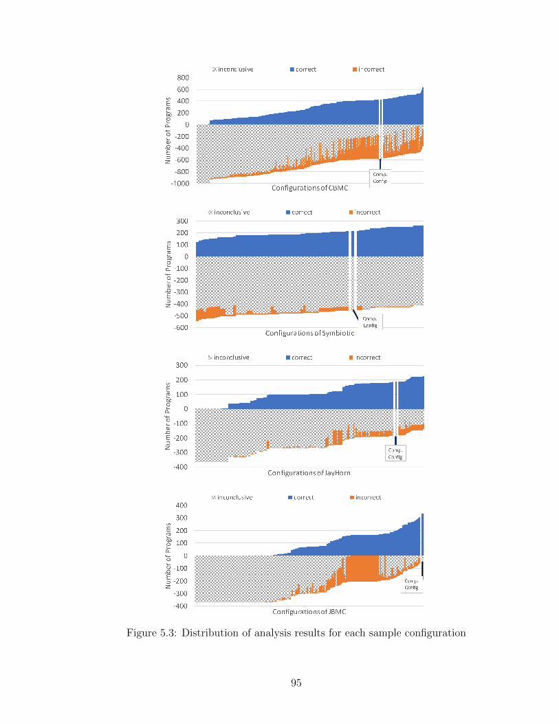
Figure 5.3: Distribution of analysis results for each sample configuration
95

dataset. Each stacked bar in Figure 5.3 corresponds to the number of verification
correct, incorrect, or incomplete analysis results with a configuration. More, the con-
figurations are ordered by the number of verification tasks they completed with the
correct result. Note that, there are many inconclusive verification runs (patterned
grey bars) for all tools. Respectively, 58%, 67%, 66%, and 62% of the verification
runs are inconclusive for CBMC , Symbiotic, JayHorn, and JBMC (third column of
Table 5.2). Maybe surprisingly, incorrect results (orange bars) are common in these
verification tools too. Respectively, 33%, 11%, 14%, and 37% of the verification
runs are incorrect for CBMC , Symbiotic, JayHorn, and JBMC (sixth and seventh
columns of Table 5.2).
In Figure 5.3, we observe large variances in the behaviors of different config-
urations. CBMC, JayHorn, and JBMC all have a number of configurations that
do not produce any conclusive results, while there exist some configurations in each
tool that can produce a few hundred correct results. The Symbiotic results have
lower variance compared to the others, but its most effective configuration (right-
most bar in the Symbiotic plot in Figure 5.3) still produces 136 more correct results
than the least effective one. Considering precision, CBMC, JayHorn, and JBMC
also have configurations that produce conclusive results for almost all the programs
at the cost of many incorrect results, demonstrating significant soundness and per-
formance tradeoffs that configuration options of these tools control.
Figure 5.3 also shows the comp-default configuration results of each tool as
the thicker bar with an arrow pointing to it. We observe that all the comp-default
configurations lead to few incorrect results, while the comp-default of CBMC, Sym-
96

biotic, and JayHorn do not lead to the largest number of correct results. Specifically,
only 1, 2, 2, and 0 incorrect results but 573, 446, 180, and 37 inconclusive results
were produced by the comp-default configurations of CBMC, Symbiotic, JayHorn,
and JBMC, respectively. This result shows that even though the comp-default
configurations have been manually tuned to reduce the number of incorrect results,
there still is room for big improvements for correctly verifying more programs.
5.5 Evaluation
5.5.1 Experimental Setup
Research Questions: We experiment with two use-case scenarios. The first sce-
nario is when a non-expert user does not know a reliable default configuration
with which to start. To simulate this scenario, we start our search with a ran-
dom configuration (with replications). We compare our search results with each
tool’s comp-default results. Recall that the comp-default of each tool was man-
ually tuned by program analysis experts for the verification tasks; therefore, this
experiment answers the following research question:
• RQ1: How close can auto-tune get to the expert knowledge starting from
random configurations?
The second scenario is when there is a reliable default configuration provided
to the user. Although often precise, the default configuration may not be conclu-
sive on many verification tasks. To simulate this scenario, we start our search with
97

each tool’s comp-default only when the configuration is inconclusive. We evalu-
ate auto-tune’s results using the scoring schema from the SV-COMP [101]. This
experiment answers the following research question:
• RQ2: Can auto-tune improve on top of expert knowledge?
Next, we conduct an in-depth investigation to explore how our approach per-
forms using the different neighbor generation strategies described in Section 5.2.3
and the different machine learning approaches described in Section 5.2.2 to answer
the following research questions:
• RQ3: How do different neighbor generation strategies affect auto-tune’s
performance?
• RQ4: How do different machine learning techniques (i.e., classification and
regression) affect auto-tune’s performance?
Numerical Value Mapping for Analysis Results: For the regression ap-
proach, we map the analysis results to the following numeric values; true negative:0,
true positive:1, inconclusive:50, false positive:99, and false negative:100. This map-
ping will also enable us to compare the training performance of both approaches
(Section 5.5.5).
Metrics: We used three metrics in our evaluation: (i) the number of correct anal-
ysis results, (ii) precision as the percentage of correct results among all conclusive
results), and (iii) the SV-COMP score.
98

Cross-validation: We perform 5-fold cross-validation by splitting the benchmark
programs into five sets and using four sets for training and one set for testing,
rotating the testing set so that each set is used for testing once.
Threshold: We experimented with five threshold values: θ = {0.1, 0.2, 0.3, 0.4, 0.5}
for classification and θ = {5, 10, 15, 20, 40} for regression.
Environment: All of our experiments were conducted on two servers. One server
has 24 Intel Xeon Silver 4116 CPUs @ 2.10GHz and 144GiB RAM, and the other
has 48 Intel Xeon Silver 4116 CPUs @ 2.10GHz and 192GiB RAM. Both servers run
Ubuntu 16.04 LTS.
Search Runs: In total, we run auto-tune for 72030 verification tasks; that is, 3
neighbor generation strategies × 2 machine learning techniques × 5 threshold values
× a total of 2401 programs (1000 and 665 C programs for CBMC and Symbiotic,
respectively, 368 programs for JayHorn and JBMC ).
5.5.2 RQ1: How close can auto-tune get to the expert knowledge?
Table 5.3 compares the auto-tune results for the first use-case scenario with
comp-default results. In this scenario, the search starts with a random configura-
tion, which can potentially have very bad performance (see Figure 5.3). Recall that
we presented multiple auto-tune settings for neighbor generation and predictive
model training that may present precision, soundness, and performance tradeoffs.
Here we analyze results and make observations about two settings: S1:base-classification
99
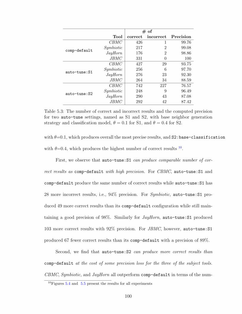
# ofTool correct incorrect Precision
comp-default
CBMC 426 1 99.76Symbiotic 217 2 99.08JayHorn 176 2 98.86JBMC 331 0 100
auto-tune:S1
CBMC 427 29 93.75Symbiotic 256 6 97.70JayHorn 276 23 92.30JBMC 264 34 88.59
auto-tune:S2
CBMC 742 227 76.57Symbiotic 248 9 96.49JayHorn 290 43 87.08JBMC 292 42 87.42
Table 5.3: The number of correct and incorrect results and the computed precisionfor two auto-tune settings, named as S1 and S2, with base neighbor generationstrategy and classification model, θ = 0.1 for S1, and θ = 0.4 for S2.
with θ=0.1, which produces overall the most precise results, and S2:base-classification
with θ=0.4, which produces the highest number of correct results 10.
First, we observe that auto-tune:S1 can produce comparable number of cor-
rect results as comp-default with high precision. For CBMC, auto-tune:S1 and
comp-default produce the same number of correct results while auto-tune:S1 has
28 more incorrect results, i.e., 94% precision. For Symbiotic, auto-tune:S1 pro-
duced 49 more correct results than its comp-default configuration while still main-
taining a good precision of 98%. Similarly for JayHorn, auto-tune:S1 produced
103 more correct results with 92% precision. For JBMC, however, auto-tune:S1
produced 67 fewer correct results than its comp-default with a precision of 89%.
Second, we find that auto-tune:S2 can produce more correct results than
comp-default at the cost of some precision loss for the three of the subject tools.
CBMC, Symbiotic, and JayHorn all outperform comp-default in terms of the num-
10Figures 5.4 and 5.5 present the results for all experiments
100

ber of correct results with 316, 38, and 114 additions; 76.57%, 96.49%, and 87.42%
precisions respectively.
We acknowledge that JBMC comp-default, as the first place winner of SV-
COMP’19, already has good performance with only 37 inconclusive results and
no incorrect results. Figure 5.3 shows that, in contrast to the other tools, JBMC
comp-default is actually the best performing configuration among the ones we used
in our experiments.
Finally, we show that auto-tune significantly outperforms the median results
of configurations in the datasets. auto-tune:S1 outperforms the dataset median
by 153, 61, 176, and 194 more correct results for CBMC, Symbiotic JayHorn, and
JBMC, respectively. The dataset median precision for these tools is 70.54, 94.76,
92.25, and 47.64 (respectively). auto-tune:S1 also outperforms these median values
with 93.75%, 97.70%, 92.30%, and 88.59% precision. This result suggests that
auto-tune can potentially improve over many configurations in the configuration
space.
Overall, we believe auto-tune can significantly improve the analysis outcomes
over many initial configurations, producing similar or more correct results than
comp-default at the cost of some precision.
5.5.3 RQ2: Can auto-tune improve on top of expert knowledge?
Figures 5.4 and 5.5 show the number of completed tasks (y-axis) for varying
threshold θ values (x-axis), for the second use-case scenario; i.e., the search runs
101
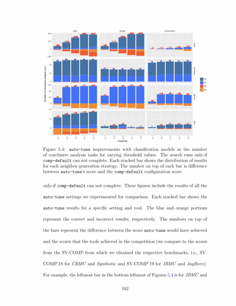
−398−398−398−398
−1218−1218−1218−1218
−2498−2498−2498−2498
−3947−3947−3947−3947 −4227−4227−4227−4227
494949555555 242424 565656 252525
−91−91−91
−230−230−230 −387−387−387 −351−351 −429−429−429
−107−107−107−107
−133−133−133−133−131−131−131−131
−113−113−113−113−80−80−80−80
−388−388−388−388
−1172−1172−1172−1172
−2553−2553−2553−2553
−3837−3837−3837−3837 −3909−3909−3909−3909
4747 4545 4545 4545 4545
−93−93
−196−196 −305−305−305 −350−350 −464−464−464
4−26−26
−26−26−26
2 −14−14
−45−45 −117−117 −171−171 −300−300 −733−733
7676 7878 7979 7878 7979
−83−83−83−83
−115−115−115−115 −98−98−98 −132−132−132−132 −281−281−281
2−26−26
−24−24 −24−24 −24−24
base greedy conservative
cbm
csym
bio
ticja
yhorn
jbm
c
0.1
0.2
0.3
0.4
0.5
0.1
0.2
0.3
0.4
0.5
0.1
0.2
0.3
0.4
0.5
−200
0
200
400
0
20
40
−40
0
40
80
120
0
10
threshold
Nu
mb
er
of
co
nclu
siv
e a
na
lysis
ru
ns
TN
TP
FN
FP
Figure 5.4: auto-tune improvements with classification models as the numberof conclusive analysis tasks for varying threshold values. The search runs only-ifcomp-default can not complete. Each stacked bar shows the distribution of resultsfor each neighbor generation strategy. The number on top of each bar is differencebetween auto-tune’s score and the comp-default configuration score.
only-if comp-default can not complete. These figures include the results of all the
auto-tune settings we experimented for comparison. Each stacked bar shows the
auto-tune results for a specific setting and tool. The blue and orange portions
represent the correct and incorrect results, respectively. The numbers on top of
the bars represent the difference between the score auto-tune would have achieved
and the scores that the tools achieved in the competition (we compare to the scores
from the SV-COMP from which we obtained the respective benchmarks, i.e., SV-
COMP’18 for CBMC and Symbiotic and SV-COMP’19 for JBMC and JayHorn).
For example, the leftmost bar in the bottom leftmost of Figures 5.4 is for JBMC and
102

−67−67−67−67−251−251−251−251
−436−436−436−436
−956−956−956−956
−2514−2514−2514−2514
3434
41413737
4343 4343
−72−72 −103−103 −136−136 −118−118
−173−173−173
−76−76−76−76 −123−123−123−123
−105−105−105−105
−91−91−91 −90−90
−36−36−36−36−150−150−150−150
−445−445−445−445
−1120−1120−1120−1120
−2392−2392−2392−2392
−42−42 −26−26−26−21−21−21 −21−21−21 −39−39
44
33 33
55 −10−10
−72−72 −32−32 −78−78 −64−64 −90−90
1717 1717 1717 1717 1717
−15−15−11−11
−14−14 −12−12 3
−29−29−29
55 6
8
−7−7−7
base greedy conservative
cbm
csym
bio
ticja
yhorn
jbm
c
5
10
15
20
40 5
10
15
20
40 5
10
15
20
40
−100
0
100
200
300
0
5
10
15
20
0
20
40
−5.0
−2.5
0.0
2.5
5.0
threshold
Nu
mb
er
of
co
nclu
siv
e a
na
lysis
ru
ns
TN
TP
FN
FP
Figure 5.5: auto-tune improvements with regression models.
auto-tune:base-classification with θ = 0.1. This run has 12 correct results,
and 8 incorrect results leading to 107 points decrease in SV-COMP’19 score over
comp-default.
For three out of four verification tools, i.e., Symbiotic, JayHorn, and JBMC,
auto-tune led to improvements in the competition score in some settings with no
additional incorrect results. The competition is scored as follows: 2 points for verifi-
cation of a safe program (i.e., a true negative or TN), 1 point for finding a bug in an
unsafe program (i.e., a true positive or TP), 0 points for an inconclusive analysis run
(i.e., unknown or UNK), -16 points for finding a non-existing bug in a safe program
(i.e., false positive or FP), and -32 for verification of an unsafe program (i.e., false
negative or FN).
103

auto-tune improves upon the scores in all Symbiotic runs from SV-COMP
with a maximum improvement of 79 points, in one JayHorn run with an improve-
ment of 3 points, and in ten JBMC runs with a maximum improvement of 8 points.
Recall that all of these improvements are significant as they improve on top of al-
ready expert-tuned configurations. Specifically, auto-tune results on JBMC mean
that we can improve upon the first place winner of SV-COMP’19, which can already
produce correct results on 90% of the programs. For CBMC, however, there was
no auto-tune run with a score improvement due to the big penalty for incorrect
results.
We also observe that auto-tune increases the number of correct results in all
runs (with the exception of the greedy-regression setting for Symbiotic). This,
however, does not mean improved competition score as auto-tune pays the large
penalty for the incorrect results in general. Last, all auto-tune settings that do not
improve the competition score have lower precision compared to their performance
in the first use-case scenario (RQ2) –including S1 and S2. This result suggests
that the tasks that comp-default configurations could not complete are harder to
analyze, and the verification tools are less likely to produce correct results for them.
5.5.4 RQ3: How do different neighbor generation strategies affect
auto-tune’s performance?
We use Figures 5.4 and 5.5 to investigate how the neighbor generation strate-
gies affect auto-tune’s performance. On the overall, the conservative strategy leads
104
to more precise analysis runs with fewer conclusive results, while the base strategy
leads to a higher number of conclusive results at the expense of lowered precision.
We now present observations about each of the individual strategies.
Base: Although the numbers of correct results are consistently high using the base
strategy, the precision is dependent on the tools. This is mostly due to the nature of
the configuration options that the tools have; i.e., some tools’ configurations are more
likely to lead to incorrect results than others (Figure 5.3). For CBMC, JayHorn, and
JBMC, all base runs had incorrect results, causing no improvement. For Symbiotic,
however, there were very few incorrect results that the score improvement stayed
positive.
Conservative: We observe that the runs using the conservative strategy achieve
high precision but produce fewer conclusive results compared to the base strategy.
All conservative runs achieve 100% precision (regression only) for Symbiotic and an
average of 94% precision for other tools. For JBMC , the conservative strategy led to
fewer conclusive results when combined with the classification approach (discussed
in Section 5.5.5).
Greedy: In greedy runs, we observe that the behavior varies. The results are
similar to the base for CBMC and JayHorn, while they are similar to conservative
for JBMC. This is attributable to the options we decide to forbid (or allow) using
the screening study findings. CBMC and JayHorn each have two option values
forbidden with the greedy strategy; therefore, the results are closer to base. While
105

for JBMC, the forbidden option value set of greedy is similar to that of conservative.
To further investigate how these strategies affect our search algorithm, Ta-
ble 5.4 shows the median number (and SIQR, in smaller font) of configurations
generated c′, accepted c, determined to be the best so far c∗, and used to run the
analysis tool (line 19 of Algorithm 2) only for the conclusive regression runs to bet-
ter isolate the effect of the strategies. When auto-tune cannot find a configuration
that leads to a conclusive result, it generates 115 124 configurations (always the
same), accepts 57 537 of them, but none of them gets used to run the analysis tool
(median). As a general trend, we observe that the search completes very quickly.
The median number of configurations generated across all search runs is 16. The
overall acceptance rate is 88%, and there is only one analysis run (last column)
per auto-tune run. These results suggest that 1) all neighbor generation strategies
could generate a new configuration that is potentially superior to the current, and
2) auto-tune can quickly locate a configuration that leads to a conclusive analysis
result.
Last, we observe no trends in the number of configurations generated, ex-
cepted, and run with each neighbor generation strategy that apply for all tools.
Therefore, we conclude by saying that the effect of the neighbor generation strategy
depends on the behavior of the configuration options the analysis tools have.
106

Neighbor # of configurationsTool strategy generated accepted best run
CBMCbase 25 28 21 21 3 2 1 0
greedy 28 28 23 22 3 2 1 0
conservative 18 25 15 20 2 1 1 0
Symbiotic
base 13 12 12 10 1 0 1 0
greedy 9 3 9 3 1 0 1 0
conservative 13 9 13 9 1 0 1 0
JayHornbase 8 10 7 8 1 0 1 0
greedy 7 7 6 5 1 0 1 0
conservative 14 18 12 15 1 0 1 0
JBMCbase 90 109 79 95 1 0 1 0
greedy 100 152 88 132 1 0 1 0
conservative 72 83 64 70 1 0 1 0
Table 5.4: The number of configurations generated (c′), accepted (c), improved thebest so far (c∗), and used for running tool.
Classification Regressioninaccuracy(%) mean abs. error
Tool fitness filter fitness filterCBMC 11.95 0.89 18.11 0.17 11.62 0.48 18.89 0.45
Symbiotic 23.39 2.42 21.09 4.60 12.70 1.23 5.24 0.82
JayHorn 24.15 1.48 32.47 1.35 13.19 0.40 17.04 1.64
JBMC 18.51 1.00 32.97 2.74 13.95 0.40 26.00 1.11
Table 5.5: Training performance.
5.5.5 RQ4: How do different machine learning techniques (i.e., clas-
sification and regression) affect auto-tune’s performance?
Now, we discuss how the two different machine learning techniques compare
using Figures 5.4 and 5.5. We observed that, overall, classification runs led to more
complete results but with less precision compared to the regression runs, while many
of the improvements we discussed in RQ2 are achieved with regression.
To better understand these results, Table 5.5 shows the inaccuracy of classifica-
107
tion and the mean absolute error of regression training, using the median and SIQR
values (in smaller font) for 25 training runs (5-fold cross-validation × 5 random
seeds). First, we see that for CBMC, JayHorn, and JBMC runs, fitness function
training has better performance than filter training. Since the fitness function model
M is trained on the entire ground truth dataset, while the filter F is trained only on
the conclusive parts of the dataset, these results suggest that the extra data avail-
able in the fitness function training have additional learnable patterns compared to
the conclusive subset for these tools. For Symbiotic, however, the trend is reversed.
The filter training has better performance than fitness function, suggesting that the
fitness function model was unable to learn any additional patterns in the conclusive
part of the datasets.
Last, although we cannot precisely compare the training performance of re-
gression and classification, we observe that for three tools, Symbiotic, JayHorn, and
JBMC, the regression error is significantly lower than the inaccuracy of classification.
5.5.6 Threats to Validity
There are several threats to the validity of our study. First, the benchmarks
may not be representative of the programs that naturally occur. They, however,
provide good coverage of program verifications scenarios by exercising a lot of intri-
cate code patterns. Also, they have been used in the annual SV-COMP for many
years to assess the performance of 30+ program verification tools.
Another threat about the size of the datasets. Our ground-truth datasets
108

consist of 55K to 295K data points, which may not be large enough to cover many
potential interactions between analysis options and program features. We plan to
address this threat by incorporating more benchmark programs into our dataset in
future work.
Next, we applied auto-tune only to four program verification tools for veri-
fying two programming languages. In the future work chapter we will discuss some
potential directions to create more ground-truth datasets cover more programming
languages. The tools we studied, however, are good representative of the state-
of-the-art in the research field implementing fundamental program analysis and
verification techniques. CBMC and JBMC implement bounded model-checking
technique for C and Java programs, respectively. JayHorn also implements a model-
checking technique using Horn clauses for Java programs. Symbiotic implements
symbolic execution11.
5.6 Attributions and Acknowledgments
The work presented in this chapter is done with collaborators Austin Mordalh,
a Ph.D. student at The University if Texas at Dallas (UTD), Dr. Shiyi Wei, and the
academic advisors of Ugur Koc. I, Ugur Koc, designed and developed the auto-tune
approach. I also designed the experimental setup and evaluation framework with
the guadiance other collaborators.
11See Appendix A for more details on the program analysis techniques
109

Chapter 6: Related Work
In this chapter, we discuss work related to the approaches we described in
Chapters 3, 4, and 5. First, we discuss research that uses machine learning to classify
false positive static analysis reports. Then, we discuss the broader application of
machine learning techniques, specifically, natural language processing (NLP), to the
source code to solve a variety of software engineering problems.
6.1 Related Work for Automatic False Positive Classification
Z-ranking by Kremenek and Engler [7] is one of the earliest approaches ad-
dressing false positive static analysis reports. The z-ranking technique ranks analysis
reports, using the frequency counts of successful and failed checks. The observations
underlying the design of the approach are that; bugs are rare, and bad analysis de-
cisions can lead to explosions of spurious false positive bug reports. Therefore, false
positive bug reports are likely to refer to more failed checks than successful ones.
Although this work provides interesting insights, it requires altering a static analy-
sis tool to gather the successful and failed checks. Furthermore, the successful and
failed checks are not well defined for all static analysis algorithms and problems.
More recent work aims to filter false positive analysis reports using machine
110

learning based on hand-engineered features [45, 46, 9, 10]. Yuksel and Sozer used
ten features, extracted from bug reports and analyzed programs, to classify static
analysis alerts for C++ programs [9]. They experiment with 34 different machine
learning algorithms and report 86% accuracy in classification. Tripp et al. simi-
larly identify 14 features for false positive XSS reports generated for JavaScript
programs. They report significant improvements in precision of the static analy-
sis using the classifiers as a post-analysis filter [10]. In our empirical assessment
(Chapter 4), we evaluated this approach by adopting these 14 features for Java pro-
grams, attempting to hew closely to the type of features used in the original work.
Our approach differs from these work in that, we do not manually extract features.
Instead, we use sophisticated machine learning techniques that can automatically
capture important signals in programs.
In a more recent study, Raghothaman et al. introduce a user-guided Bayesian
inference approach to filter false positive reports from deductive rule-based static
analysis algorithms [114]. We did not include this work in our evaluation because it
works on a per-program basis, requires user input, and is designed for certain static
analysis techniques.
To the best of our knowledge, there are no prior empirical studies of machine
learning approaches for false positive static analysis report classification. Further-
more, none of the existing work in this line of research has studied our second
application scenario, which focuses on demonstrating the generalizability of the ma-
chine learning models. Next, we discuss the broader application of natural language
processing techniques to software engineering problems.
111

6.2 Natural Language Processing (NLP) Techniques Applied to Code
NLP techniques achieved a great level of success for the tasks involving daily
life language because it is repetitive and predictable. Hindle et al. [115] used NLP
techniques on source code, arguing that source code written by human developers is
similarly repetitive and predictable as well. Therefore, NLP techniques can poten-
tially be very successful in learning properties from code. Expending on this work,
multiple researchers have successfully applied NLP techniques to programs to tackle
a wide range of software engineering problems such as clone detection [116], API
mining [117, 118], variable naming and renaming [119, 120], code suggestion and
completion [121, 122, 123], bug detection [75].
Nguyen et al. [122] introduce a new statistical semantic language modeling for
source code to handle some development tasks like code suggestion and completion.
Tu et al. [121] add a cache component into the n-gram model to exploit local prop-
erties in the code. Raychev et al. [123] use n-gram and neural network language
models for code completion for API calls. Allamanis et al. [120] propose a new
neural network-based model with word embeddings to suggest meaningful method
and class names for Java code. In another related work, Allamanis et al. [124] use
a deep convolutional neural network for source code summarization (a sort natural
language summary for a method/function). Fowkes et al. [118] learn API usage
patterns using probabilistic modeling. Gu et al. [125] solve the same problem using
a deep recurrent neural network. White et al. [116] use recurrent neural networks
(i.e., like our work) to detect code clones.
112

Above, we listed some sample work that demonstrated the successful appli-
cation of NLP techniques for source code processing to solve software engineering
problems. This list, however, is not meant to be comprehensive. For more compre-
hensive coverage of the literature, we refer the readers to the recent survey of such
research efforts by Allamanis et al. [126]. Note that none of the mentioned work
solves the false error report classification problem.
6.3 Selection and Ranking of Static Analyses
Next, we discuss the related work for the auto-tune approach. To the best
of our knowledge, ours is the first work to use machine learning to select a good
configuration of a tool that is likely to lead to the desired analysis result for a
given verification task. However, we find two lines of research closely related to our
approach: (i) selection and ranking of static analyses; (ii) adaptive static analysis
techniques.
The applications most relevant to our work are the papers that select strategies
within a static analysis tool [100, 127], and those that rank static analysis tools based
on their likelihood of producing the desirable analysis result for a given task [30,
31, 128]. Beyer and Dangl presented a feature-based approach to select from three
manually-defined verification strategies for CPAchecker [129, 100]. A strategy
is a sequence of verifiers defined within CPAchecker. Their approach uses four
boolean program features to define the selection heuristic. Richter and Wehrheim
presented PeSCo, an approach that uses a machine learning model to predict the
113

best ordering of five CPAchecker strategies [127]. Although these two studies
are addressing a related problem, our approach differs from them in two aspects.
First, our meta-heuristic search algorithm leverages machine learning models that
are applicable to different static analysis tools. Second, the large configuration space
of static analysis tools presents a challenge that drives us to design an efficient
search-based algorithm.
Tulsian et al. presented Mux to select the optimal verification tools to run on
Windows device drivers [30]. Their learning-based approach trains Support Vector
Machine (SVM) and regression models on a verification repository to generate an
algorithm selector. Then Mux extracts features from the device driver to be verified
and uses an algorithm selector that predicts the optimal tool to run on it. The focus
of the prediction is running time. In our work, we focus on the large configuration
space of static analysis tools and predict the configuration that is likely to lead to
conclusive and correct results.
Czech et al. presented a method to predict the rankings of SV-COMP tools
using a machine learning approach [31]. They use kernel methods to predict rank-
ings based on a graph representation of verification tasks. Similarly, Demyanova
et al. presented a feature-based machine learning method to construct a portfolio
solver [128]. The portfolio solver uses heuristic preprocessing to select one of the
existing tools and demonstrates that their approach would hypothetically win both
SV-COMP 2014 and 2015. The above approaches focus on selecting from a list
of available tools, while our research complements these work by considering the
configurability of each static analysis tool.
114

6.4 Adaptive Sensitivity Static Analysis
Several recent research studies have focused on predicting sensitivity of an
analysis algorithm to be selectively applied on the target program. Context-sensitivity
is the mostly studied analysis option [21, 22, 24, 25]. Very simply, context-sensitivity
is about how to analyze each method in a program. Analyzing the method only once,
independent of the context it is called with would be context-insensitive but fast,
while analyzing a method separately for each context it is called with would be
context-sensitive but very expensive.
Jeong et al. presented an approach to automatically determine which parts
of a program to apply context-sensitivity [24]. They hand-engineered low-level,
easy-to-obtain features in Java methods and statements. They then developed a
learning model that synthesized high-level features by combining low-level features
with boolean formulae, and then returned a parameterized heuristic function that
indicates the level of context-sensitivity necessary for each method. Similarly, Li
et al. presented Scaler, a scalable pointer analysis framework with self-tuning
context-sensitivity [22]. Scaler allows the user to specify a maximum size of the
points-to information generated, and then performs the most precise analysis within
that memory bound. It achieves this by running an inexpensive pre-analysis that
extracts information sufficient to make an estimate of how expensive various context-
sensitivities would be on different program methods. Scaler then selects a context-
sensitivity level such that a precise analysis is yielded while still falling within the
specified memory bound. Li et al. also presented a method to automatically intro-
115

duce context-sensitivity as needed on parts of programs into an otherwise context-
insensitive analysis [25]. The authors manually identified three value-flow patterns,
then constructed Zipper, which recognizes these patterns in Java code and guides
analysis by identifying methods that would benefit from context-sensitivity. Wei
and Ryder presented an adaptive context-sensitive analysis for JavaScript [21].
They extracted eight features of JavaScript functions from the points-to graph
and call graph and then developed learning-based heuristics informing how those
eight features should affect the choice of context-sensitivity. Their adaptive analysis
then uses these heuristics and the extracted features to choose a context-sensitive
analysis for each function. Other analysis options, such as flow-sensitivity, have also
been used to develop selective static analysis (e.g., [23]). Our work similarly stud-
ies the relationship between program features and analysis algorithms to achieve a
good balance between performance, precision, and soundness. But we consider a
wide range of configuration options, while all the work mentioned above focuses on
certain analysis algorithms and configuration options. In addition, instead of de-
veloping a selective analysis, our approach aims to help the users of existing static
analysis tools by automatically configuring the tools.
Another research area combining machine learning and program analysis is
using machine learning to learn a static analysis. Oh, Yang, and Yi presented a
strategy for using Bayesian optimization to learn the parts of a program to which
one should apply precision-improving techniques when performing static analysis
[23]. Their approach extracts features from variables in the program to determine
which of those variables would benefit the most from higher-precision analyses and
116

then applies those analyses to some number of those features.
Smaragdakis et al. observed that unsoundness is necessary in order to scale
static analyses [20]. Heo, Oh, and Yi observed that this unsoundness is uniform in
modern bug-detecting static analyses, causing a high number of false alarms. They
presented a method to use machine learning to selectively make a static analysis
unsound over certain loops in a program [130]. They trained classifiers to identify
harmless loops (i.e., loops that, when analyzed unsoundly, reduce false positives and
introduce no false negatives) in the programs under analysis. The classifier then
identifies harmless loops in programs, which the analyzer unrolls once and replaces
with an if-statement. Instead of modifying an existing static analysis algorithm or
designing new analysis algorithms, our approaches focus on improving the usability
of existing static analysis tools.
117

Chapter 7: Conclusion
In this dissertation, we presented machine learning-based approaches to ad-
dress two critical usability issues that static analysis tools face: false positive results
and proper tool configuration.
False positive reports are one of the major reasons developers give for not using
them in their software development practice [1]. To address this issue, we presented
a learning approach to find program structures that cause the state-of-the-art static
analysis tools to emit false error reports, and to filter out such false error reports
with a classifier trained on the code (Chapter 3) [71]. In particular, we designed
and developed two machine learning models: a Bayesian inference-based model and
an LSTM model; and two code reduction techniques: method body and backward
slice.
To evaluate the effectiveness of the approach, we conducted a case study of a
widely-used static analysis tool for Java web security checks, i.e., FindSecBugs. In
the case study, we discovered interesting signals involving Java collection objects
with the Naive Bayes model. Investigating these signals, we found that FindSecBugs
cannot successfully reason about very simple usage scenarios of Java collection
objects like HashMap and ArrayList. FindSecBugs likely considers the entire data
118

collection as tainted if there are any tainted objects put into the collection. This
over-approximation results in many false positive reports, which can be avoided if
static analysis developers improve their analysis of collection classes in the future.
With the LSTM model, we achieved 89.6% and 85% accuracy in classification for
the method body and the backward slice datasets, respectively. In fact, using the
LSTM model trained on the backward slice dataset as a false positive result filter, we
removed 81% of the false positives from the developers’ view, while only mistakenly
removing 2.7% of real bug reports, which improved the tool’s overall precision from
49.6% to 90.5%.
Furthermore, we analyzed the output LSTM produced for the tokens of two
input programs. With this analysis, we (i) showed that long-term dependencies
exist in the data, (ii) demonstrated LSTMs’ capability of inferring the context in
which the tokens appear, and (iii) showed how LSTMs output values agree with the
findings of Naive Bayes model.
We believed the results of this case study suggested that the approach was
promising. Therefore, we extended the approach and the empirical evaluations in
several ways (Chapter 4) [18]. We presented the first empirical study that evaluates
four families of machine learning approaches, i.e., HEF, BoW, LSTM, and GGNN,
for classifying static analysis reports to filter false positives from true positives.
Moreover, we introduced new code transformation routines for preparing programs
as inputs to these machine learning approaches.
We used three datasets in our experiments. The first dataset is built from the
OWASP benchmark using the SQL injection vulnerabilities only (the same dataset
119

we used in the case study in Section 3.3). The other two datasets are built from
the real-world benchmark programs we collected for this study. To create these
datasets, we manually reviewed 400 analysis reports to label them as true or false
positive. In this manual review process, we made two critical observations about the
scenarios in which false positives occur. These observations suggest that it is crucial
to create more real-world benchmarks to assess static analysis tools and machine
learning-based approaches like ours.
We compared 13 machine learning approaches from four families using the
OWASP and real-world datasets under two application scenarios. The results of our
experiments suggest that the LSTM approach generally achieves better accuracy.
We also observed that, across all approaches, the second application scenario in
which the training is done with one set of programs, and the models are tested on
other programs is more challenging. It requires learning the symptoms of true/false
positive reports that hold across programs. All of the learning approaches performed
significantly lower in this application scenario compared to the first application sce-
nario in which training and test samples coming from the same programs. Particu-
larly in this application scenario, we observed that more detailed data preparation
with abstraction and word extraction leads to significant increases in accuracy while
not causing any significant drops in the first application scenario. LSTM, the best
performing model, achieved slightly above 80% accuracy in classification with very
precise data preparation in this application scenario. We also showed that there
could be a higher variance in recall and precision than in accuracy. We conjecture
this is because the recall and precision are not directly related to the loss function
120

being optimized in training.
Overall, the results of our empirical evaluations suggest that we can effectively
distinguish and filter out a majority of false positive bug reports without drastically
affecting the number of true bug reports.
Next, we addressed the configurability challenge of static analysis tools (Chap-
ter 5). We presented auto-tune, a meta-heuristic search approach to automatically
configure static analysis tools. This approach is novel in that it uses machine learn-
ing models both as fitness functions to explore large configuration spaces and as
filters to avoid selecting expensive analysis runs that will likely produce false results.
Note that these filters are very much like the false positive classification models we
learned in Chapters 3 and 4. There are two key differences, however; (i) in addition
to the program representations, they also learn about the tool configurations and
(ii) instead of just a classification result, they output a continues numeric score.
We applied auto-tune to four popular verification tools: CBMC and Symbi-
otic for C programs; JayHorn and JBMC Java programs, and evaluated its per-
formance compared to how these tools did in the software verification competition
SV-COMP in two scenarios. In the first scenario, starting the search with a ran-
dom configuration, we examined how close auto-tune’s performance can get to the
expert knowledge by taking the competition configurations of these subject tools,
i.e., comp-default, as the reference point for the expert knowledge. We found that
auto-tune was able to select configurations comparable to comp-default. For three
out of the four subjects, auto-tune could increase the number of correct analysis
results with a reasonably small loss in precision. The other subject, JBMC , had
121

already completed 94% tasks correctly, which is a very high percentage.
In the second scenario, we run the search only if the comp-default configu-
ration fails to produce a conclusive analysis result. In this case, auto-tune could
increase the number of correct analysis results for all subjects. For three subjects,
these improvements also translated into SV-COMP score improvements in some set-
tings of auto-tune. For one subject, CBMC , however, there was no auto-tune run
with SC-COMP score improvement due to the substantial penalty for the few false
results auto-tune generated.
We further investigated the impact of two design choices of the auto-tune
approach: neighbor generation strategy, and machine learning model (for varying
threshold values). For neighbor generation, we observe that the conservative strat-
egy leads to more precise analysis runs with fewer conclusive results, while the base
strategy leads to a higher number of conclusive results at the expense of drops in
precision. For the machine learning models, the classification runs led to more com-
plete results but with less precision compared to the regression runs, while many
of the improvements we discussed in RQ2 are achieved with regression. Overall,
the results of the empirical evaluations suggest that the auto-tune approach can
improve the performance of program verification tools by automatically configuring
them for given verification tasks.
We believe that the approaches we proposed, developed, and empirically eval-
uated will help software developers to incorporate static tools into their development
practice, i.e., improving the adoption of the verification tools. Furthermore, the in-
sights we gathered through dataset creation and empirical evaluations will also help
122

static analysis developers to enhance the performance of their tools.
123

Chapter 8: Future Work
In the chapter we discuss potential directions for future work to extend the
approaches we presented. We start with false positive detection.
8.1 Future Work for False Positive Detection
The major limitation for extending the research in this direction is the avail-
ability of ground-truth datasets. The research community needs, but currently lacks,
an extensive repository of real-word datasets to enable new research into machine
learning-based approaches to program analysis and understanding. We created an
example dataset of this kind and used it in our systematic assessment study [18]. The
results of this study and further observations we made underlined the significance
of having real-world examples. However, this dataset was a somewhat ad-hoc at-
tempt, and no individual effort will be sufficient to create such a repository datasets
at scale. The research community needs to pay attention to this shortcoming.
An exciting research direction to create such datasets is to study crowdsourc-
ing techniques. Crowdsourcing has already been well-studied and used for many
software engineering problems [131]. There are vast online communities formed
124

around crowdsourcing platforms like Topcoder1 and bugcrowd2. Similar platforms
can be promising for creating these datasets.
Once the datasets are created, further machine learning studies can be done.
For instance, we believe recursive neural networks [132] can be useful for learning
on abstract syntax tree (AST) representation of the code. Also, although we experi-
mented with GNNs, their complexity might require learning with larger datasets for
tuning the hyper-parameters effectively. Therefore, further investigation of GNNs
with more data is necessary.
Moreover, as we discussed in Chapter 2, different machine learning algorithms
have different biases and therefore their performance can be dependent on the nature
of data. Another potential direction is to explore these biases and the nature of the
data for combining different machine learning approaches with a voting scheme.
Last, the approaches we presented can be extended to become a semi-supervised
incremental online service that static analysis developers and users can use to im-
prove the tools quality, performance, and thereby practicality.
8.2 Future Work for auto-tune
The availability of real-world datasets is a limitation also for this work. Other
than crowdsourcing direction, program analysis competitions like SV-COMP [101]
present an excellent opportunity to extend the datasets to cover more kinds of
software bugs and programming languages.
1https://www.topcoder.com2https://www.bugcrowd.com
125
With the availability of more datasets, we think of two potential directions to
extend the auto-tune approach. The first direction involves designing and develop-
ing more sophisticated machine learning architectures that can learn more structural
information from programs’ code, along with the configuration options of the anal-
ysis tools. The second direction involves integrating more search algorithms into
auto-tune, such as A* search, genetic algorithms, and tabu search [133], to see
whether the configuration space can be explored more efficiently and effectively. To
adopt simulated annealing, we incorporated two machine learning models both as
fitness functions and false result filters. Other search algorithms might, however,
require designing other machine learning-based components.
126

Appendix A: Program Analysis Techniques
This appendix provides brief background information on the program anal-
ysis techniques implemented or used the static analysis tools we have studied in
Chapters 3, 4, and 5.
A.1 Taint Analysis
1 public class MyServlet extends HttpServlet {
2 public void doPost(HttpServletRequest request){
3 String param = "";
4 Enumeration<String> headers = request.getHeaders("OFFSET");
5 if (headers.hasMoreElements()) {
6 param = headers.nextElement(); // tainted data
7 }
8 String sql = "SELECT id, name FROM products ORDER BY name
LIMIT 20 OFFSET " + param;
9 Connection con = DatabaseHelper.getConnection();
10 con.prepareCall(sql).execute(); // security-critical
operation on database
11 } // end doPost
12 } /* end class*/
Figure A.1: An example code vulnerable for SQL injection.
Taint analysis can be seen as a form of information flow analysis. Information
flow can happen with any operation (or series of operations) that uses the value of
an object to derive a value for another. In this flow, if the source of the flow is
127

untrustworthy, we call the value coming from that source “tainted”. Taint analysis
aims at tracking the propagation of such tainted values in a program.
A highly popular application of this technique is to perform security checks
against injection attacks. With taint analysis, static analysis tools can check If
tainted values can reach to security-critical operations in a program. For example,
running an SQL query on the database is usually a security-critical operation, and
data received from untrustworthy resources should not be used to create SQL state-
ments without proper sanitization. Consider the short program in Figure A.1. This
program is vulnerable to SQL injection attacks. The tainted value received from an
HTTP request object has been used to create an SQL statement that gets executed
on the database (respectively, at lines 7, 10, and 12). FndSecBugs, the subject static
analysis tool in Chapters 3 and 4, can effectively find such security vulnerabilities
with taint analysis.
A.2 Model-checking
Model-checking [134] is a program analysis (a formal method more specifi-
cally) technique that uses finite-state models (FSM) of software programs to check
the correctness properties for given specifications written in propositional temporal
logic [135]. Model-checking tools exhaustively search the state space to find paths
from start states to invalid states. If such paths exist, the tool can also provide a
counter-example that shows how to reach to the invalid state.
However, model-checking tools face a combinatorial blow-up of the state space
128

as the programs get bigger. One common approach to address this issue is to bound
the number of steps taken on the FSM. This approach is called bounded model-
checking (BMC). CBMC [99] and JBMC [36] implement this approach to verify (or
to find bugs in) C and Java programs.
JayHorn also implements model-checking for specification violations in Java
programs. JayHorn generates constrained Horn clauses (CHC) [136] as verification
conditions and passes them to a Horn engine that checks their satisfiability. CHCs
are rule-like logic formulae specifying the pre-conditions on the parameters of meth-
ods, post-conditions on return values of methods, and list of variables in the scope
for each program location.
A.3 Symbolic Execution
Symbolic execution is a technique for analyzing a program to determine what
inputs cause each part of a program to execute. Symbiotic implements the symbolic
execution technique to verify (or to find bugs in) C programs. Symbiotic interprets a
given program by assuming symbolic values for inputs rather than obtaining concrete
inputs as normal program execution would (like running a test case). Symbiotic
computes expressions of the inputs in terms of those symbols for the expressions
and variables in the program. These expressions are called path-conditions, and
they denote the possible outcomes of each conditional branch in the program.
129

Bibliography
[1] Brittany Johnson, Yoonki Song, Emerson Murphy-Hill, and Robert Bowdidge.Why Don’T Software Developers Use Static Analysis Tools to Find Bugs? InProceedings of the 2013 International Conference on Software Engineering,ICSE ’13, pages 672–681, Piscataway, NJ, USA, 2013. IEEE Press.
[2] Guy Erez, Eran Yahav, and Mooly Sagiv. Generating concrete counterexam-ples for sound abstract interpretation. Citeseer, 2004.
[3] Xavier Rival. Understanding the Origin of Alarms in Astree. In Static Anal-ysis, Lecture Notes in Computer Science, pages 303–319. Springer, Berlin,Heidelberg, September 2005.
[4] Bhargav S. Gulavani and Sriram K. Rajamani. Counterexample Driven Re-finement for Abstract Interpretation. In Tools and Algorithms for the Con-struction and Analysis of Systems, Lecture Notes in Computer Science, pages474–488. Springer, Berlin, Heidelberg, March 2006.
[5] Youil Kim, Jooyong Lee, Hwansoo Han, and Kwang-Moo Choe. Filteringfalse alarms of buffer overflow analysis using SMT solvers. Information andSoftware Technology, 52(2):210–219, February 2010.
[6] Benjamin Livshits, Manu Sridharan, Yannis Smaragdakis, Ondrej Lhotak,J Nelson Amaral, Bor-Yuh Evan Chang, Samuel Z Guyer, Uday P Khedker,Anders Møller, and Dimitrios Vardoulakis. In Defense of Soundiness: A Man-ifesto. Communications of the ACM, 58(2):44–46, 2015.
[7] Ted Kremenek and Dawson Engler. Z-ranking: Using Statistical Analysisto Counter the Impact of Static Analysis Approximations. In Proceedings ofthe 10th International Conference on Static Analysis, SAS’03, pages 295–315,Berlin, Heidelberg, 2003. Springer-Verlag.
[8] Yungbum Jung, Jaehwang Kim, Jaeho Shin, and Kwangkeun Yi. TamingFalse Alarms from a Domain-Unaware C Analyzer by a Bayesian StatisticalPost Analysis. In Static Analysis, Lecture Notes in Computer Science, pages203–217. Springer, Berlin, Heidelberg, September 2005.
130

[9] U. Yuksel and H. Sozer. Automated Classification of Static Code AnalysisAlerts: A Case Study. In 2013 IEEE International Conference on SoftwareMaintenance, pages 532–535, September 2013.
[10] Omer Tripp, Salvatore Guarnieri, Marco Pistoia, and Aleksandr Aravkin.ALETHEIA: Improving the Usability of Static Security Analysis. In Proceed-ings of the 2014 ACM SIGSAC Conference on Computer and CommunicationsSecurity, CCS ’14, pages 762–774, New York, NY, USA, 2014. ACM.
[11] Ugur Koc, Parsa Saadatpanah, Jeffrey S. Foster, and Adam A. Porter. Learn-ing a Classifier for False Positive Error Reports Emitted by Static Code Anal-ysis Tools. In Proceedings of the 1st ACM SIGPLAN International Workshopon Machine Learning and Programming Languages, MAPL 2017, pages 35–42,New York, NY, USA, 2017. ACM.
[12] Philippe Arteau. Find Security Bugs, version 1.4.6, 2015. http://find-sec-bugs.
github.io, Accessed on 2018-01-04.
[13] The OWASP Foundation. The OWASP Benchmark for Security Automation,version 1.1, 2014. https://www.owasp.org/index.php/Benchmark, Accessed on 2018-01-04.
[14] Sepp Hochreiter and Jurgen Schmidhuber. Long short-term memory. NeuralComputation, 9(8):1735, November 1997.
[15] Felix A. Gers, JAŒrgen Schmidhuber, and Fred Cummins. Learning to Forget:Continual Prediction with LSTM. Neural Computation, 12(10):2451–2471,October 2000.
[16] Alex Graves. Supervised Sequence Labelling. In Supervised Sequence Labellingwith Recurrent Neural Networks, Studies in Computational Intelligence, pages5–13. Springer, Berlin, Heidelberg, 2012.
[17] James Bergstra, Olivier Breuleux, Frederic Bastien, Pascal Lamblin, Raz-van Pascanu, Guillaume Desjardins, Joseph Turian, David Warde-Farley, andYoshua Bengio. Theano: A cpu and gpu math compiler in python. In Proc.9th Python in Science Conf, volume 1, pages 3–10, 2010.
[18] Ugur Koc, Shiyi Wei, Jeffrey S Foster, Marine Carpuat, and Adam A Porter.An empirical assessment of machine learning approaches for triaging reports ofa java static analysis tool. In 2019 12th IEEE Conference on Software Testing,Validation and Verification (ICST), pages 288–299. IEEE, 2019.
[19] Shiyi Wei, Piotr Mardziel, Andrew Ruef, Jeffrey S. Foster, and Michael Hicks.Evaluating design tradeoffs in numeric static analysis for java. In Program-ming Languages and Systems - 27th European Symposium on Programming,ESOP 2018, Held as Part of the European Joint Conferences on Theory andPractice of Software, ETAPS 2018, Thessaloniki, Greece, April 14-20, 2018,Proceedings, pages 653–682, 2018.
131
[20] Yannis Smaragdakis, George Kastrinis, and George Balatsouras. Introspec-tive analysis: Context-sensitivity, across the board. In Proceedings of the 35thACM SIGPLAN Conference on Programming Language Design and Imple-mentation, PLDI ’14, pages 485–495, New York, NY, USA, 2014. ACM.
[21] Shiyi Wei and Barbara G. Ryder. Adaptive context-sensitive analysis forjavascript. In 29th European Conference on Object-Oriented Programming,ECOOP 2015, July 5-10, 2015, Prague, Czech Republic, pages 712–734, 2015.
[22] Yue Li, Tian Tan, Anders Møller, and Yannis Smaragdakis. Scalability-firstpointer analysis with self-tuning context-sensitivity. In Proceedings of the 201826th ACM Joint Meeting on European Software Engineering Conference andSymposium on the Foundations of Software Engineering, ESEC/FSE 2018,pages 129–140, New York, NY, USA, 2018. ACM.
[23] Hakjoo Oh, Hongseok Yang, and Kwangkeun Yi. Learning a strategy foradapting a program analysis via bayesian optimisation. In Proceedings of the2015 ACM SIGPLAN International Conference on Object-Oriented Program-ming, Systems, Languages, and Applications, OOPSLA 2015, pages 572–588,New York, NY, USA, 2015. ACM.
[24] Sehun Jeong, Minseok Jeon, Sungdeok Cha, and Hakjoo Oh. Data-driven context-sensitivity for points-to analysis. Proc. ACM Program. Lang.,1(OOPSLA):100:1–100:28, October 2017.
[25] Yue Li, Tian Tan, Anders Møller, and Yannis Smaragdakis. Precision-guided context sensitivity for pointer analysis. Proc. ACM Program. Lang.,2(OOPSLA):141:1–141:29, October 2018.
[26] Ugur Koc, Shiyi Wei, Jeffrey S. Foster, Marine Carpuat, and Adam A. Porter.An empirical assessment of machine learning approaches for triaging reportsof a java static analysis tool. In 12th IEEE Conference on Software Testing,Validation and Verification, ICST 2019, Xi’an, China, April 22-27, 2019,pages 288–299, 2019.
[27] Enas A Alikhashashneh, Rajeev R Raje, and James H Hill. Using machinelearning techniques to classify and predict static code analysis tool warnings.In 2018 IEEE/ACS 15th International Conference on Computer Systems andApplications (AICCSA), pages 1–8. IEEE, 2018.
[28] Sunghun Kim and Michael D Ernst. Which warnings should i fix first? InProceedings of the the 6th joint meeting of the European software engineeringconference and the ACM SIGSOFT symposium on The foundations of softwareengineering, pages 45–54. ACM, 2007.
[29] Sarah Heckman and Laurie Williams. On establishing a benchmark for evalu-ating static analysis alert prioritization and classification techniques. In Pro-ceedings of the Second ACM-IEEE international symposium on Empirical soft-ware engineering and measurement, pages 41–50. ACM, 2008.
132

[30] Varun Tulsian, Aditya Kanade, Rahul Kumar, Akash Lal, and Aditya V Nori.Mux: algorithm selection for software model checkers. In Proceedings of the11th Working Conference on Mining Software Repositories, pages 132–141.ACM, 2014.
[31] Mike Czech, Eyke Hullermeier, Marie-Christine Jakobs, and Heike Wehrheim.Predicting Rankings of Software Verification Tools. In Proceedings of the 3rdACM SIGSOFT International Workshop on Software Analytics, SWAN 2017,pages 23–26, New York, NY, USA, 2017. ACM.
[32] Rakefet Ackerman and Valerie A Thompson. Meta-reasoning. Reasoning asmemory, pages 164–182, 2015.
[33] Stefania Costantini. Meta-reasoning: a survey. In Computational Logic: LogicProgramming and Beyond, pages 253–288. Springer, 2002.
[34] Jirı Slaby, Jan Strejcek, and Marek Trtık. Checking properties described bystate machines: On synergy of instrumentation, slicing, and symbolic execu-tion. In International Workshop on Formal Methods for Industrial CriticalSystems, pages 207–221. Springer, 2012.
[35] Jiri Slaby, Jan Strejcek, and Marek Trtık. Symbiotic: synergy of instrumen-tation, slicing, and symbolic execution. In International Conference on Toolsand Algorithms for the Construction and Analysis of Systems, pages 630–632.Springer, 2013.
[36] Lucas Cordeiro, Pascal Kesseli, Daniel Kroening, Peter Schrammel, and MarekTrtik. JBMC: A bounded model checking tool for verifying Java bytecode. InComputer Aided Verification (CAV), volume 10981 of LNCS, pages 183–190.Springer, 2018.
[37] Temesghen Kahsai, Philipp Rummer, Huascar Sanchez, and Martin Schaf.Jayhorn: A framework for verifying java programs. In International Confer-ence on Computer Aided Verification, pages 352–358. Springer, 2016.
[38] Mohamad Kassab, Joanna F DeFranco, and Phillip A Laplante. Softwaretesting: The state of the practice. IEEE Software, 34(5):46–52, 2017.
[39] Kshirasagar Naik and Priyadarshi Tripathy. Software testing and quality as-surance: theory and practice. John Wiley & Sons, 2011.
[40] Srinivasan Desikan and Gopalaswamy Ramesh. Software testing: principlesand practice. Pearson Education India, 2006.
[41] Caitlin Sadowski, Edward Aftandilian, Alex Eagle, Liam Miller-Cushon, andCiera Jaspan. Lessons from building static analysis tools at google. Commu-nications of the ACM (CACM), 61 Issue 4:58–66, 2018.
133

[42] Caitlin Sadowski, Jeffrey Van Gogh, Ciera Jaspan, Emma Soderberg, andCollin Winter. Tricorder: Building a program analysis ecosystem. In Proceed-ings of the 37th International Conference on Software Engineering-Volume 1,pages 598–608. IEEE Press, 2015.
[43] Junjie Wang, Song Wang, and Qing Wang. Is there a ”golden” feature set forstatic warning identification?: An experimental evaluation. In Proceedings ofthe 12th ACM/IEEE International Symposium on Empirical Software Engi-neering and Measurement, ESEM ’18, pages 17:1–17:10, New York, NY, USA,2018. ACM.
[44] Stuart J Russell and Peter Norvig. Artificial intelligence: a modern approach.Malaysia; Pearson Education Limited,, 2016.
[45] S. S. Heckman. Adaptive probabilistic model for ranking code-based staticanalysis alerts. In Software Engineering - Companion, 2007. ICSE 2007 Com-panion. 29th International Conference on, pages 89–90, May 2007.
[46] Sarah Smith Heckman. A systematic model building process for predictingactionable static analysis alerts. North Carolina State University, 2009.
[47] Yoav Goldberg. Neural network methods for natural language processing.Synthesis Lectures on Human Language Technologies, 10(1):1–309, 2017.
[48] A. Sureka and P. Jalote. Detecting Duplicate Bug Report Using Character N-Gram-Based Features. In 2010 Asia Pacific Software Engineering Conference,pages 366–374, November 2010.
[49] Stacy K. Lukins, Nicholas A. Kraft, and Letha H. Etzkorn. Bug localiza-tion using latent Dirichlet allocation. Information and Software Technology,52(9):972 – 990, 2010.
[50] Xin Ye, Hui Shen, Xiao Ma, Razvan Bunescu, and Chang Liu. From WordEmbeddings to Document Similarities for Improved Information Retrieval inSoftware Engineering. In Proceedings of the 38th International Conference onSoftware Engineering, ICSE ’16, pages 404–415, New York, NY, USA, 2016.ACM.
[51] Danilo P Mandic and Jonathon Chambers. Recurrent neural networks forprediction: learning algorithms, architectures and stability. John Wiley &Sons, Inc., 2001.
[52] Felix A GERS, Jurgen SCHMIDHUBER, and Fred CUMMINS. Learning toforget: Continual prediction with lstm. Neural computation, 12(10):2451–2471,2000.
[53] Razvan Pascanu, Tomas Mikolov, and Yoshua Bengio. Understanding theexploding gradient problem. CoRR, abs/1211.5063, 2, 2012.
134

[54] Tomas Mikolov, Martin Karafiat, Lukas Burget, Jan Cernocky, and SanjeevKhudanpur. Recurrent neural network based language model. In EleventhAnnual Conference of the International Speech Communication Association,2010.
[55] Tomas Mikolov and Geoffrey Zweig. Context dependent recurrent neural net-work language model. SLT, 12(234-239):8, 2012.
[56] Kyunghyun Cho, Bart Van Merrienboer, Caglar Gulcehre, Dzmitry Bahdanau,Fethi Bougares, Holger Schwenk, and Yoshua Bengio. Learning phrase rep-resentations using rnn encoder-decoder for statistical machine translation.arXiv:1406.1078, 2014.
[57] Hoa Khanh Dam, Truyen Tran, and Trang Thi Minh Pham. A deep lan-guage model for software code. In FSE 2016: Proceedings of the FoundationsSoftware Engineering International Symposium, pages 1–4, 2016.
[58] Nate Kushman and Regina Barzilay. Using semantic unification to generateregular expressions from natural language. In Proceedings of the 2013 Con-ference of the North American Chapter of the Association for ComputationalLinguistics: Human Language Technologies, pages 826–836, 2013.
[59] Wang Ling, Phil Blunsom, Edward Grefenstette, Karl Moritz Hermann,Tomas Kocisky, Fumin Wang, and Andrew Senior. Latent predictor networksfor code generation. In Proceedings of the 54th Annual Meeting of the As-sociation for Computational Linguistics (Volume 1: Long Papers), volume 1,pages 599–609, 2016.
[60] Marco Gori, Gabriele Monfardini, and Franco Scarselli. A new model forlearning in graph domains. In Neural Networks, 2005. IJCNN’05. Proceed-ings. 2005 IEEE International Joint Conference on, volume 2, pages 729–734.IEEE, 2005.
[61] F. Scarselli, M. Gori, A. C. Tsoi, M. Hagenbuchner, and G. Monfardini.The Graph Neural Network Model. IEEE Transactions on Neural Networks,20(1):61–80, January 2009.
[62] Zachary Reynolds, Abhinandan Jayanth, Ugur Koc, Adam Porter, RajeevRaje, and James Hill. Identifying and documenting false positive patternsgenerated by static code analysis tools. In 4th International Workshop OnSoftware Engineering Research And Industrial Practice, 2017.
[63] Mark Weiser. Program slicing. In Proceedings of the 5th international confer-ence on Software engineering, pages 439–449. IEEE Press, 1981.
[64] IBM. The T.J.Watson Libraries for Analysis (WALA), 2006. http://wala.
sourceforge.net/wiki/index.php, Accessed on 2018-01-04.
135

[65] Pierre-Luc Carrier and Kyunghyun Cho. Lstm Networks for Sentiment Anal-ysis, 2016. http://deeplearning.net/tutorial/lstm.html, Accessed on 2018-01-04.
[66] Matthew D. Zeiler. ADADELTA: An Adaptive Learning Rate Method.arXiv:1212.5701 [cs], December 2012.
[67] Nathaniel Ayewah and William Pugh. Using Checklists to Review Static Anal-ysis Warnings. In Proceedings of the 2Nd International Workshop on Defectsin Large Software Systems: Held in Conjunction with the ACM SIGSOFTInternational Symposium on Software Testing and Analysis (ISSTA 2009),DEFECTS ’09, pages 11–15, New York, NY, USA, 2009. ACM.
[68] Tim Boland and Paul E Black. Juliet 1.1 c/c++ and java test suite. Computer,45(10):0088–90, 2012.
[69] Robert A Martin. Common weakness enumeration. Mitre Corporation, 2007.https://cwe.mitre.org, Accessed on 2018-01-04.
[70] Andrej Karpathy, Justin Johnson, and Li Fei-Fei. Visualizing and Understand-ing Recurrent Networks. arXiv:1506.02078, June 2015.
[71] Ugur Koc, Parsa Saadatpanah, Jeffrey S. Foster, and Adam A. Porter. Learn-ing a classifier for false positive error reports emitted by static code analysistools. In Proceedings of the 1st ACM SIGPLAN International Workshop onMachine Learning and Programming Languages, MAPL 2017, pages 35–42,New York, NY, USA, 2017. ACM.
[72] Joana (java object-sensitive analysis) - information flow control framework forjava. https://pp.ipd.kit.edu/projects/joana.
[73] B. K. Rosen, M. N. Wegman, and F. K. Zadeck. Global value numbers andredundant computations. In Proceedings of the 15th ACM SIGPLAN-SIGACTSymposium on Principles of Programming Languages, POPL ’88, pages 12–27,New York, NY, USA, 1988. ACM.
[74] Yujia Li, Daniel Tarlow, Marc Brockschmidt, and Richard Zemel. GatedGraph Sequence Neural Networks. arXiv:1511.05493 [cs, stat], November2015. arXiv: 1511.05493.
[75] Miltiadis Allamanis, Marc Brockschmidt, and Mahmoud Khademi. Learningto Represent Programs with Graphs. arXiv:1711.00740 [cs], November 2017.arXiv: 1711.00740.
[76] Tomas Mikolov, Kai Chen, Greg Corrado, Jeffrey Dean, L Sutskever, andG Zweig. word2vec. https://code.google.com/p/word2vec, 2013.
[77] Yoav Goldberg and Omer Levy. word2vec explained: deriving mikolov et al.’snegative-sampling word-embedding method. arXiv:1402.3722, 2014.
136

[78] Elisa Burato, Pietro Ferrara, and Fausto Spoto. Security analysis of the owaspbenchmark with julia. In Proc. of ITASEC17, the rst Italian Conference onSecurity, Venice, Italy, 2017.
[79] Achilleas Xypolytos, Haiyun Xu, Barbara Vieira, and Amr MT Ali-Eldin.A framework for combining and ranking static analysis tool findings basedon tool performance statistics. In Software Quality, Reliability and SecurityCompanion (QRS-C), 2017 IEEE International Conference on, pages 595–596.IEEE, 2017.
[80] Apollo: a distributed configuration center, 2018. https://github.com/ctripcorp/
apollo, Accessed on 2019-06-02.
[81] Andreas Prlic, Andrew Yates, Spencer E Bliven, Peter W Rose, Julius Ja-cobsen, Peter V Troshin, Mark Chapman, Jianjiong Gao, Chuan Hock Koh,Sylvain Foisy, et al. Biojava: an open-source framework for bioinformatics in2012. Bioinformatics, 28(20):2693–2695, 2012.
[82] Free chat-server: A chatserver written in java. https://sourceforge.net/projects/
freecs, Accessed on 2019-09-10.
[83] Giraph : Large-scale graph processing on hadoop. http://giraph.apache.org.
[84] H2 database engine. http://www.h2database.com, Accessed on 2019-06-02.
[85] Apache jackrabbit is a fully conforming implementation of the content reposi-tory for java technology api. http://jackrabbit.apache.org, Accessed on 2019-06-02.
[86] Hypersql database. http://hsqldb.org, Accessed on 2019-06-02.
[87] Jetty: lightweight highly scalable java based web server and servlet engine,2018. https://www.eclipse.org/jetty, Accessed on 2019-06-02.
[88] Joda-time a quality replacement for the java date and time classes. http:
//www.joda.org/joda-time, Accessed on 2019-06-02.
[89] Java pathfinder. https://github.com/javapathfinder, Accessed on 2019-06-02.
[90] Mybatis: Sql mapper framework for java. http://www.mybatis.org/mybatis-3, Ac-cessed on 2019-06-02.
[91] Okhttp: An http & http/2 client for android and java applications. http:
//square.github.io/okhttp, Accessed on 2019-06-02.
[92] Adrian Smith. Universal password manager. http://upm.sourceforge.net, Accessedon 2019-06-02.
[93] Susi.ai - Software and Rules for Personal Assistants. http://susi.ai, Accessed on2019-06-02.
137

[94] Stephen M. Blackburn, Robin Garner, Chris Hoffmann, Asjad M. Khang,Kathryn S. McKinley, Rotem Bentzur, Amer Diwan, Daniel Feinberg, DanielFrampton, Samuel Z. Guyer, Martin Hirzel, Antony Hosking, Maria Jump,Han Lee, J. Eliot B. Moss, Aashish Phansalkar, Darko Stefanovic, ThomasVanDrunen, Daniel von Dincklage, and Ben Wiedermann. The DaCapoBenchmarks: Java Benchmarking Development and Analysis. In Proceedingsof the 21st Annual ACM SIGPLAN Conference on Object-oriented Program-ming Systems, Languages, and Applications, OOPSLA ’06, pages 169–190,New York, NY, USA, 2006. ACM.
[95] Andrew Johnson, Lucas Waye, Scott Moore, and Stephen Chong. Exploringand Enforcing Security Guarantees via Program Dependence Graphs. In Pro-ceedings of the 36th ACM SIGPLAN Conference on Programming LanguageDesign and Implementation, PLDI ’15, pages 291–302, New York, NY, USA,2015. ACM.
[96] Ugur Koc and Cemal Yilmaz. Approaches for computing test-case-aware cov-ering arrays. Software Testing, Verification and Reliability, 28(7):e1689, 2018.
[97] Frank Eibe, MA Hall, and IH Witten. The weka workbench. Morgan Kauf-mann, 2016.
[98] Microsoft gated graph neural networks. https://github.com/Microsoft/
gated-graph-neural-network-samples, Accessed on 2018-09-02.
[99] Daniel Kroening and Michael Tautschnig. Cbmc–c bounded model checker. InInternational Conference on Tools and Algorithms for the Construction andAnalysis of Systems, pages 389–391. Springer, 2014.
[100] Dirk Beyer and Matthias Dangl. Strategy Selection for Software VerificationBased on Boolean Features. In Tiziana Margaria and Bernhard Steffen, edi-tors, Leveraging Applications of Formal Methods, Verification and Validation.Verification, Lecture Notes in Computer Science, pages 144–159. Springer In-ternational Publishing, 2018.
[101] Dirk Beyer. Software verification with validation of results. In InternationalConference on Tools and Algorithms for the Construction and Analysis ofSystems, pages 331–349. Springer, 2017.
[102] Grigorios Tsoumakas and Ioannis Katakis. Multi-label classification: Anoverview. International Journal of Data Warehousing and Mining (IJDWM),3(3):1–13, 2007.
[103] Scott Kirkpatrick, C Daniel Gelatt, and Mario P Vecchi. Optimization bysimulated annealing. science, 220(4598):671–680, 1983.
[104] Peter JM Van Laarhoven and Emile HL Aarts. Simulated annealing. Springer,1987.
138

[105] Vincent Granville, Mirko Krivanek, and J-P Rasson. Simulated annealing:A proof of convergence. Pattern Analysis and Machine Intelligence, IEEETransactions on, 16(6):652–656, 1994.
[106] The llvm compiler infrastructure. https://llvm.org, Accessed on 2019-10-02.
[107] Ronald Aylmer Fisher. Design of experiments. Br Med J, 1(3923):554–554,1936.
[108] John Sall, Mia L Stephens, Ann Lehman, and Sheila Loring. JMP start statis-tics: a guide to statistics and data analysis using JMP. Sas Institute, 2017.
[109] Mark Hall, Eibe Frank, Geoffrey Holmes, Bernhard Pfahringer, Peter Reute-mann, and Ian H Witten. The weka data mining software: an update. ACMSIGKDD explorations newsletter, 11(1):10–18, 2009.
[110] Leo Breiman. Random forests. Machine learning, 45(1):5–32, 2001.
[111] MBA Snousy, HM El-Deeb, K Badran, and IAA Khlil. Suite of decisiontree-based classification algorithms on cancer gene expression data. egyptianinformatics journal 12 (2): 73–82, 2011.
[112] Changhai Nie and Hareton Leung. A survey of combinatorial testing. ACMComputing Surveys, 43:11:1–11:29, February 2011.
[113] C. Yilmaz, S. Fouche, M. B. Cohen, A. Porter, G. Demiroz, and U. Koc.Moving Forward with Combinatorial Interaction Testing. Computer, 47(2):37–45, February 2014.
[114] Mukund Raghothaman, Sulekha Kulkarni, Kihong Heo, and Mayur Naik.User-guided program reasoning using bayesian inference. In Proceedings ofthe 39th ACM SIGPLAN Conference on Programming Language Design andImplementation, PLDI 2018, pages 722–735, New York, NY, USA, 2018. ACM.
[115] Abram Hindle, Earl T. Barr, Zhendong Su, Mark Gabel, and PremkumarDevanbu. On the Naturalness of Software. In Proceedings of the 34th Inter-national Conference on Software Engineering, pages 837–847, Piscataway, NJ,USA, 2012. IEEE Press.
[116] Martin White, Michele Tufano, Christopher Vendome, and Denys Poshyvanyk.Deep Learning Code Fragments for Code Clone Detection. In Proceedings ofthe 31st IEEE/ACM International Conference on Automated Software Engi-neering, ASE 2016, pages 87–98, New York, NY, USA, 2016. ACM.
[117] Xiaodong Gu, Hongyu Zhang, Dongmei Zhang, and Sunghun Kim. Deepapi learning. In Proceedings of the 2016 24th ACM SIGSOFT InternationalSymposium on Foundations of Software Engineering, pages 631–642. ACM,2016.
139

[118] Jaroslav Fowkes and Charles Sutton. Parameter-free Probabilistic API MiningAcross GitHub. In Proceedings of the 2016 24th ACM SIGSOFT InternationalSymposium on Foundations of Software Engineering, FSE 2016, pages 254–265, New York, NY, USA, 2016. ACM.
[119] Veselin Raychev, Martin Vechev, and Andreas Krause. Predicting ProgramProperties from ”Big Code”. In Proceedings of the 42Nd Annual ACMSIGPLAN-SIGACT Symposium on Principles of Programming Languages,POPL ’15, pages 111–124, New York, NY, USA, 2015. ACM.
[120] Miltiadis Allamanis, Earl T. Barr, Christian Bird, and Charles Sutton. Sug-gesting Accurate Method and Class Names. In Proceedings of the 2015 10thJoint Meeting on Foundations of Software Engineering, ESEC/FSE 2015,pages 38–49, New York, NY, USA, 2015. ACM.
[121] Zhaopeng Tu, Zhendong Su, and Premkumar Devanbu. On the Localness ofSoftware. In Proceedings of the 22Nd ACM SIGSOFT International Sympo-sium on Foundations of Software Engineering, FSE 2014, pages 269–280, NewYork, NY, USA, 2014. ACM.
[122] Tung Thanh Nguyen, Anh Tuan Nguyen, Hoan Anh Nguyen, and Tien N.Nguyen. A Statistical Semantic Language Model for Source Code. In Proceed-ings of the 2013 9th Joint Meeting on Foundations of Software Engineering,ESEC/FSE 2013, pages 532–542, New York, NY, USA, 2013. ACM.
[123] Veselin Raychev, Martin Vechev, and Eran Yahav. Code Completion with Sta-tistical Language Models. In Proceedings of the 35th ACM SIGPLAN Confer-ence on Programming Language Design and Implementation, PLDI ’14, pages419–428, New York, NY, USA, 2014. ACM.
[124] Miltiadis Allamanis, Hao Peng, and Charles Sutton. A Convolutional Atten-tion Network for Extreme Summarization of Source Code. arXiv:1602.03001[cs], February 2016.
[125] Xiaodong Gu, Hongyu Zhang, Dongmei Zhang, and Sunghun Kim. Deep APILearning. arXiv:1605.08535 [cs], May 2016.
[126] Miltiadis Allamanis, Earl T. Barr, Premkumar Devanbu, and Charles Sutton.A survey of machine learning for big code and naturalness. ACM Comput.Surv., 51(4):81:1–81:37, July 2018.
[127] Cedric Richter and Heike Wehrheim. Pesco: Predicting sequential combina-tions of verifiers. In International Conference on Tools and Algorithms for theConstruction and Analysis of Systems, pages 229–233. Springer, 2019.
[128] Yulia Demyanova, Thomas Pani, Helmut Veith, and Florian Zuleger. Empir-ical software metrics for benchmarking of verification tools. Formal Methodsin System Design, 50(2):289–316, June 2017.
140

[129] Dirk Beyer and M Erkan Keremoglu. Cpachecker: A tool for configurablesoftware verification. In International Conference on Computer Aided Verifi-cation, pages 184–190. Springer, 2011.
[130] Kihong Heo, Hakjoo Oh, and Kwangkeun Yi. Machine-learning-guided Se-lectively Unsound Static Analysis. In Proceedings of the 39th InternationalConference on Software Engineering, ICSE ’17, pages 519–529, Piscataway,NJ, USA, 2017. IEEE Press.
[131] T. D. LaToza and A. van der Hoek. Crowdsourcing in Software Engineering:Models, Motivations, and Challenges. IEEE Software, 33(1):74–80, January2016.
[132] Richard Socher, Cliff C Lin, Chris Manning, and Andrew Y Ng. Parsingnatural scenes and natural language with recursive neural networks. In Pro-ceedings of the 28th international conference on machine learning (ICML-11),pages 129–136, 2011.
[133] Duc Pham and Dervis Karaboga. Intelligent optimisation techniques: geneticalgorithms, tabu search, simulated annealing and neural networks. SpringerScience & Business Media, 2012.
[134] Edmund M Clarke Jr, Orna Grumberg, Daniel Kroening, Doron Peled, andHelmut Veith. Model checking. MIT press, 2018.
[135] Pierre Wolper. Expressing interesting properties of programs in propositionaltemporal logic. In POPL, volume 86, pages 184–193, 1986.
[136] Peter Padawitz. Computing in Horn clause theories, volume 16. SpringerScience & Business Media, 2012.
141