Embed Size (px)
Citation preview

ABSTRACT
Title of dissertation: Fully Anisotropic Solution of the Three DimensionalBoltzmann Transport Equation
Francis G. VanGessel, Masters of Science, 2016
Thesis directed by: Professor Peter W. ChungDepartment of Mechanical Engineering
The development of accurate modeling techniques for nanoscale thermal trans-
port is an active area of research. Modern day nanoscale devices have length scales
of tens of nanometers and are prone to overheating, which reduces device perfor-
mance and lifetime. Therefore, accurate temperature profiles are needed to predict
the reliability of nanoscale devices. The majority of models that appear in the liter-
ature obtain temperature profiles through the solution of the Boltzmann transport
equation (BTE). These models often make simplifying assumptions about the nature
of the quantized energy carriers (phonons). Additionally, most previous work has
focused on simulation of planar two dimensional structures. This thesis presents
a method which captures the full anisotropy of the Brillouin zone within a three
dimensional solution to the BTE. The anisotropy of the Brillouin zone is captured
by solving the BTE for all vibrational modes allowed by the Born Von-Karman
boundary conditions.

Table of Contents
List of Tables iv
List of Figures v
1 Introduction 11.1 Perspective and Motivation . . . . . . . . . . . . . . . . . . . . . . . 11.2 Scope of Thesis . . . . . . . . . . . . . . . . . . . . . . . . . . . . . . 5
2 Literature Review 82.1 First Principles Calculations . . . . . . . . . . . . . . . . . . . . . . . 92.2 Molecular Dynamics . . . . . . . . . . . . . . . . . . . . . . . . . . . 102.3 Boltzmann Transport Equation . . . . . . . . . . . . . . . . . . . . . 13
2.3.1 Monte Carlo Method . . . . . . . . . . . . . . . . . . . . . . . 142.3.2 Equation of Phonon Radiative Transfer . . . . . . . . . . . . . 162.3.3 Lattice Boltzmann Method . . . . . . . . . . . . . . . . . . . . 17
3 Theory 193.1 Direct Space Lattice . . . . . . . . . . . . . . . . . . . . . . . . . . . 193.2 Reciprocal Space Lattice and Brillouin Zone . . . . . . . . . . . . . . 223.3 Lattice Dynamics . . . . . . . . . . . . . . . . . . . . . . . . . . . . . 23
3.3.1 1-D Example . . . . . . . . . . . . . . . . . . . . . . . . . . . 273.3.2 Vibrational Properties . . . . . . . . . . . . . . . . . . . . . . 31
3.4 Quantum Nature of Phonons . . . . . . . . . . . . . . . . . . . . . . . 353.5 Determination of Allowed Wavevectors . . . . . . . . . . . . . . . . . 38
4 Boltzmann Transport Solver Algorithm 454.1 Boltzmann Solver Inputs . . . . . . . . . . . . . . . . . . . . . . . . . 45
4.1.1 Frequencies and Group Velocities . . . . . . . . . . . . . . . . 464.1.2 Relaxation Times . . . . . . . . . . . . . . . . . . . . . . . . . 49
4.2 Discretization . . . . . . . . . . . . . . . . . . . . . . . . . . . . . . . 534.2.1 Specific Heat . . . . . . . . . . . . . . . . . . . . . . . . . . . 594.2.2 Boundary Conditions . . . . . . . . . . . . . . . . . . . . . . . 61
4.2.2.1 Fourier Interface Condition . . . . . . . . . . . . . . 62
ii

4.2.2.2 Specular Scattering Condition . . . . . . . . . . . . . 634.2.2.3 Diffuse Scattering Condition . . . . . . . . . . . . . . 63
4.2.3 Computational Implementation . . . . . . . . . . . . . . . . . 65
5 Simulations and Results 725.1 Semi-Ballistic Transport . . . . . . . . . . . . . . . . . . . . . . . . . 72
5.1.1 Verification Problem Set-Up . . . . . . . . . . . . . . . . . . . 735.1.2 Verification Results . . . . . . . . . . . . . . . . . . . . . . . . 78
5.2 Effect of Anisotropy . . . . . . . . . . . . . . . . . . . . . . . . . . . 825.3 FinFET Design and Self-Heating . . . . . . . . . . . . . . . . . . . . 94
5.3.1 Problem Set-Up . . . . . . . . . . . . . . . . . . . . . . . . . . 955.3.2 Device Simulation Results . . . . . . . . . . . . . . . . . . . . 103
6 Conclusion 1126.1 Closure . . . . . . . . . . . . . . . . . . . . . . . . . . . . . . . . . . . 1126.2 Future Work . . . . . . . . . . . . . . . . . . . . . . . . . . . . . . . . 114
Bibliography 116
iii

List of Tables
4.1 Relaxation time parameters . . . . . . . . . . . . . . . . . . . . . . . 53
5.1 Gray phonon properties . . . . . . . . . . . . . . . . . . . . . . . . . 785.2 Lennard Jones parameters . . . . . . . . . . . . . . . . . . . . . . . . 975.3 Scattering rates ( [1]) . . . . . . . . . . . . . . . . . . . . . . . . . . . 995.4 Scattering rate parameters ( [1]) . . . . . . . . . . . . . . . . . . . . . 995.5 Maximum temperature rise . . . . . . . . . . . . . . . . . . . . . . . . 1075.6 Phonon mode properties . . . . . . . . . . . . . . . . . . . . . . . . . 109
iv

List of Figures
1.1 FinFET schematic . . . . . . . . . . . . . . . . . . . . . . . . . . . . 7
3.1 Two dimensional crystal . . . . . . . . . . . . . . . . . . . . . . . . . 203.2 Cubic lattice structures . . . . . . . . . . . . . . . . . . . . . . . . . . 213.3 First Brillouin zone of a FCC lattice . . . . . . . . . . . . . . . . . . 243.4 Visual description of dynamical matrix . . . . . . . . . . . . . . . . . 273.5 One dimensional chain with two atom basis . . . . . . . . . . . . . . 283.6 Dispersion relations of linear chain . . . . . . . . . . . . . . . . . . . 333.7 Group velocities of linear chain . . . . . . . . . . . . . . . . . . . . . 353.8 Wave and particle representations of phonons . . . . . . . . . . . . . 383.9 Periodic boundary conditions . . . . . . . . . . . . . . . . . . . . . . 39
4.1 RDX unit cell . . . . . . . . . . . . . . . . . . . . . . . . . . . . . . . 474.2 Three phonon interactions . . . . . . . . . . . . . . . . . . . . . . . . 524.3 Simulation domain . . . . . . . . . . . . . . . . . . . . . . . . . . . . 554.4 Upwinding . . . . . . . . . . . . . . . . . . . . . . . . . . . . . . . . . 584.5 Specular reflection . . . . . . . . . . . . . . . . . . . . . . . . . . . . 644.6 Diffuse reflection . . . . . . . . . . . . . . . . . . . . . . . . . . . . . 644.7 Parallelization process . . . . . . . . . . . . . . . . . . . . . . . . . . 684.8 Boltzmann transport solver flow chart . . . . . . . . . . . . . . . . . . 70
5.1 Plane parallel dimensions and temperature profile . . . . . . . . . . . 745.2 Method of succesive approximations flow chart . . . . . . . . . . . . . 765.3 Spherical Brillouin zone . . . . . . . . . . . . . . . . . . . . . . . . . 775.4 Temperature profile for Kn = 10 . . . . . . . . . . . . . . . . . . . . . 795.5 Temperature profile for Kn = 2 . . . . . . . . . . . . . . . . . . . . . 795.6 Temperature profile for Kn = 1 . . . . . . . . . . . . . . . . . . . . . 805.7 Temperature profile for Kn = 1/2 . . . . . . . . . . . . . . . . . . . . 805.8 Mesh convergence study . . . . . . . . . . . . . . . . . . . . . . . . . 815.9 Silicon dispersion along Γ−X . . . . . . . . . . . . . . . . . . . . . . 835.10 Frequency contours of the kz = 0 plane of the Brillouin zone . . . . . 845.11 Iso-frequency surface of TA branch in Brillouin zone . . . . . . . . . . 855.12 Group velocities of iso-frequency contours in kz = 0 plane . . . . . . . 87
v

5.13 Simulation domain for anisotropy study . . . . . . . . . . . . . . . . . 885.14 Temperature contours for isotropic simulation . . . . . . . . . . . . . 905.15 Temperature contours for anisotropic simulation . . . . . . . . . . . . 915.16 Difference between isotropic and anisotropic simulations . . . . . . . 925.17 Percent difference between isotropic and anisotropic simulations . . . 935.18 Idealized Simple Cubic Lattice . . . . . . . . . . . . . . . . . . . . . . 965.19 Dispersion curves for LJ solid . . . . . . . . . . . . . . . . . . . . . . 985.20 Evolution of carrier concentration with applied gate voltage ( [3]) . . 1005.21 Three channel geometries simulated in FinFET device . . . . . . . . . 1015.22 Thin Fin . . . . . . . . . . . . . . . . . . . . . . . . . . . . . . . . . . 1025.23 Medium Fin . . . . . . . . . . . . . . . . . . . . . . . . . . . . . . . . 1025.24 Thick Fin . . . . . . . . . . . . . . . . . . . . . . . . . . . . . . . . . 1025.25 Boundary conditions applied to the simulation domain . . . . . . . . 1035.26 Temperature profiles for channel 1 . . . . . . . . . . . . . . . . . . . . 1055.27 Temperature profiles for channel 2 . . . . . . . . . . . . . . . . . . . . 1065.28 Temperature profiles for channel 1 . . . . . . . . . . . . . . . . . . . . 1085.29 Energy profiles of mode 1 and mode 2 . . . . . . . . . . . . . . . . . . 110
vi

Chapter 1: Introduction
1.1 Perspective and Motivation
Moore’s Law states that the number of transistors on an integrated circuit
doubles roughly every two years. This qualitative law has been the driving force
behind the rapid increase in processor speeds over the past few decades. One result
of the increase in transistor density is an increase in the power generated on an
integrated circuit. Although in general the power generated per transistor shrinks
as the transistor characteristic dimensions are reduced, this effect is counterbalanced
by the increase of the overall number of transistors on an integrated circuit, leading
to an overall power generation increase. Furthermore, in order to double the number
of transistors on an integrated circuit, the size of a transistor must be reduced. The
most recent generation of transistors have gate lengths of 14 nanometers [4] with
the next generation reaching even smaller lengths. This size reduction results in
hotspot creation within the transistor where heat is trapped and cannot be efficiently
removed [5–9]. These self heating effects are exacerbated in devices with non-planar
three dimensional geometries. The combined effects of increasing power density
coupled with shrinking feature size leads to inefficient heat removal, resulting in
large increases in temperature which negatively effects device performance. Among
1

these negative effects are reductions in saturation currents and maximum allowable
frequencies which reduce the transistors operating performance [10]. Furthermore,
the strain caused by overheating reduces the transistor lifetime [11]. Therefore,
accurate thermal modeling is critical for determining device reliability in existing
devices as well as designing transistors which minimize hotspot temperatures.
Continuum laws, such as Fourier’s Law of heat conduction, rely on the assump-
tion that a material may be assumed homogeneous on the length scale of interest.
In addition, these laws assume that local equilibrium is assumed to prevail through-
out the material. When devices, such as transistors, have characteristic dimensions
within the nanometer regime, sub-continuum effects begin to dominate and the as-
sumptions underlying continuum laws are no longer valid. Therefore modeling tech-
niques that are capable of capturing subcontinuum effects are required for accurate
prediction of temperature profiles within such nanoscale devices. One such mod-
eling technique is the solution of the Boltzmann transport equation which may be
numerically solved to determine a wide range of thermodynamic properties, includ-
ing temperature profiles, in devices with dimensions ranging from a few nanometers
up through the macroscale. The Boltzmann transport equation is an appealing
technique as it is capable of capturing ballistic transport effects that emerge on
the atomistic scale, while also accurately modeling regions where diffusive transport
dominates. Thus the Boltzmann transport equation is a widely used method for
simulation of nanoscale devices and thin crystalline films.
Despite gaining widespread use for nanoscale thermal modeling, methods for
the numerical solution of the Boltzmann transport equation detailed in the liter-
2

ature often have a variety of simplifying assumptions that limit the accuracy of
the solutions obtained. Chief amongst these are the gray and semi-gray approxi-
mation which assume that the energy carriers, henceforth referred to as phonons,
within a crystalline material may be approximated by a few averaged phonon prop-
erties [12–18]. More recently, work done in the area of nanoscale thermal modeling
has replaced the gray approximation with a Boltzmann transport equation formula-
tion that accounts for variation in the phonon properties, however this variation is
considered along only a single high symmetry direction in the Brillouin Zone (region
of reciprocal space containing all unique vibrational modes that exist within a mate-
rial) [19–25]. Therefore, energy transport is assumed to be isotropic, an assumption
that has been shown to be inaccurate in the literature [26]. Other assumptions
made in the literature assume that temperature varies in only one or two dimen-
sions, leading to Boltzmann transport solution methods that are unable to model
new device geometries that are intrinsically three dimensional. Examples of such
devices are new transistor designs such as the Fin field effect transistor (FinFET)
first developed at Berkeley [27] and gaining adoption in present day commercial
integrated circuits [4]. Additionally, few published methods for solving the Boltz-
mann transport equation rigorously account for the effect of material geometry on
the allowed vibrational modes. Those that do, do not consider temperature varia-
tion in three dimensions [26, 28]. While the simplifications and assumptions listed
here do not apply to all of the Boltzmann transport solution methods appearing
in the literature, no method has appeared in the literature which has completely
eliminated all of the simplifications documented above.
3

In this thesis an algorithm for solving the Boltzmann transport equation is
presented. This approach is then implemented into a numerical Boltzmann trans-
port equation code capable of three dimensional device simulation. The algorithm
presented in this thesis avoids simplifying assumptions, which appear in approaches
detailed in the literature, in order to fully capture the wide array of phonon physics.
Full Brillouin zone anisotropy is accounted for by determining phonon properties
throughout the Brillouin zone, not just along one high symmetry directions. To
this end, phonon properties are determined via a molecular dynamics approach for
obtaining lattice vibrational properties which are then used as inputs to the Boltz-
mann transport code. Secondly, the Boltzmann transport equation is discretized in
a manner allowing for three dimensional temperature gradients. This is important
as recent nanoscale devices are no longer planar, i.e. approximately two dimensional,
and therefore require three dimensional modeling. Finally the algorithm solves the
Boltzmann transport equation for all available vibrational modes within a material
by considering the device geometry. Therefore, the approach detailed in this work
is capable of capturing effects such as the reduction in thermal conductivity which
is known to occur in devices with very thin dimensions [26].
By eliminating the various simplifications and assumptions that appear in
much of the modeling methods utilizing the Boltzmann transport equation, a Boltz-
mann transport code is formulated that is capable of accurately modeling heat flow
in nanoscale crystalline devices. The scope and structure of this thesis is now pre-
sented.
4

1.2 Scope of Thesis
The remainder of this work is organized as follows. First, current computa-
tional modeling techniques for nanoscale thermal transport are reviewed in Ch. 2.
These techniques can be roughly categorized as first principles methods, molecular
dynamics methods, and Boltzmann transport simulations. The strengths, weak-
nesses, and regime of applicability for each technique is covered. Boltzmann trans-
port equation algorithms that appear in literature are discussed in more detail in
order to distinguish how the method presented in this thesis differs from existing
methodologies.
Following the literature review, the fundamentals of lattice dynamics and
phonon physics theory are presented in Ch. 3. Important concepts related to vibra-
tional modes in crystalline materials as well as nanoscale energy transport are dis-
cussed. Examples of several key concepts are presented via simple one-dimensional
examples, which avoids obfuscating the underlying physics. The concepts covered
in the theoretical section, though not complete, form the basis for understanding
the algorithm presented in later sections.
Chapter 4 details the Boltzmann transport equation algorithm as it has been
implemented into a FORTRAN90 code. First the molecular dynamics simula-
tions used for generating phonon inputs are discussed as well as the basis for the
form of the phonon relaxation times. Subsequently, the numerical discretization of
the Boltzmann transport equation is presented. The control volume discretization
scheme is briefly discussed as well as the upwinding approximation for discretizing
5

the spatial operator. The computational implementation of various boundary con-
ditions are detailed and supported through physical arguments. Finally, specifics
to the computational implementation, such as parallelization techniques and the
iterative solver, are discussed.
A variety of simulation results are presented in Ch. 5. First a simulation of
semi-ballistic transport is performed via the plane parallel problem borrowed from
the field of radiation transport physics. The simulation results are then compared
to known semi-analytical solutions in order to verify the BTE code. Once the
mathematical accuracy of the algorithm has been verified, the improvement over
existing computational techniques is demonstrated. This is shown through simple
transport problem highlighting the result of accounting for Brillouin zone anisotropy.
The final set of simulations is a parameter study of a nanoscale transistor device
known as a FinFET, a schematic of a FinFET is presented in Fig. 1.1. This device
is gaining adoption in top of the line integrated circuits, and due to the nanometer
dimensions and non-planar geometry requires modeling which accounts for three
dimensional temperature gradients as well as anisotropy in the heat flow.
The final section reiterates the main points of the thesis. The improvements
demonstrated by the algorithm are restated. In addition a path forward is detailed
for improving the method through inclusion of material interfaces, time stepping,
and OpenMPI parallelization.
6

Figure 1.1: Schematic of a typical FinFET device. The dimensions are in units ofnanometers and are obtained from [29].
7

Chapter 2: Literature Review
Modeling of subcontinuum effects is important for predicting thermal behavior
of nanoscale devices, the length and time scales of interest render experimental
techniques difficult or infeasible for many cases. Rapid increase in computing power
over the past few decades has allowed for increasingly complex computational models
of nanoscale heat transport. Computational models are not hindered by the practical
restrictions of experimental techniques attempting to probe nanometer length scales
or picosecond time scales and thus present an attractive alternative to experiment.
In addition computational techniques are inexpensive as computing time is cheaper
and often faster than experimental alternatives, albeit with reduced accuracy.
There exist a wide range of computational methods for modeling thermal be-
havior at the nanoscale. Within the next section these various computational meth-
ods will be detailed; with special attention paid to methods similar to the one utilized
in this work so that differences may be clearly stated. Each method has inherent
strengths and weaknesses as well as different length scales at which the method is
applicable. The three main computational methods that will be discussed are: first-
principles calculations, Molecular Dynamics simulations, the Boltzmann transport
equation.
8

2.1 First Principles Calculations
First principles or Ab-Initio methods seek to directly apply physical equations
and concepts to systems of interest. One manner in which Ab-Initio methods are
used in the context of determining vibrational and heat transport properties at
the nanoscale, is through determination of the exact response of electrons in the
crystal to displacements of atomic nuclei. The electronic response yields parameter
free force constants, which in turn allows for the determination of vibrational and
transport properties [30]. Alternatively if the system is sufficiently one dimensional
and without impurities, Landauer Formalism may be used to calculate heat flow.
The most prevalent computational methods for determining electronic re-
sponse for use in the first principles framework is Density Functional Theory (DFT),
and the closely related Density Functional Perturbation Theory (DFPT) [31–35].
DFT allows for calculation of the ground state electronic structure for a many body
system, which allows for direct calculation of phonon properties such as phonon
frequencies, heat capacity, and harmonic force constants [33]. DFPT extends this
approach to calculate higher order perturbations to the system in order to extract
anharmonic force constants as well as phonon lifetimes [36]. Phonon properties ob-
tained from DFT and DFPT are most often used as inputs for the determination of
thermal conductivity within the first principles framework [37]. Furthermore, these
properties may be used as inputs to the Boltzmann transport equation for accurate
device modeling. DFT/DFPT calculations may be performed using open source
computer codes such as Quantum Espresso [38], however calculation is restricted to
9

structures with a small number of atoms and becomes prohibitively computationally
expensive for large systems.
Another first principles technique that is prevalent for the prediction of nanoscale
thermal transport is the Landauer formula. The Landauer formula allows for the pre-
diction of the heat current in nanojunctions. This has application to one-dimensional
systems such as nanowires and nanotubes [39]. The fundamental quantity of im-
portance in determining the thermal current is determination of the transmission
coefficient which describes how efficiently thermal energy is transported through a
junction connected to two thermal leads. The transmission coefficient is dependent
on the thermal properties of the material of interest [40]. One method of calculating
the transmission coefficient is through non-equilibrium Green’s function. Landauer
formalism, as this approach is called, is valid when there are hundreds of atoms,
or fewer, between the two leads. At this length scale energy is transported via
waves and the phonon particle viewpoint is not necessarily valid. However, use of
the Landauer formula is restricted to small system sizes that are predominantly
one-dimensional [39].
2.2 Molecular Dynamics
Molecular dynamics is another commonly used method for nanoscale heat
transport. The molecular dynamics method uses an analytic equation describing the
interatomic potential of a material to integrate the Newtonian equations of motion,
allowing for the evolution of atomic nuclei in time and space. By treating the atomic
10

nuclei as hard spheres, which evolve according to Newtonian equations of motion,
molecular dynamics is a classical method and therefore one must exercise caution
as to the regime it is applied. In the case of lattice thermal conductivity it has been
found that molecular dynamics simulations compare well with experiment down
to one-tenth of the Debye temperature of a material [41]. Molecular dynamics by
design models the dynamics of individual atoms and has a wide range of applications
such as thermal transport, molecular assembly, chemical reactions, and material
fracture [42–47].
An important consideration when performing a molecular dynamics simulation
of thermal transport is in selecting the appropriate interatomic potential. Empirical
potentials often include fitting parameters which are fitted through comparison of
quantities such as melting temperature, lattice constant, or liquid structure to known
experimental data. However, an empirical potential which accurately predicts the
melting point of a crystal may not accurately predict the same crystal’s phonon
transport properties. Therefore, recent work has focused on fitting existing empirical
potentials to certain properties that better predict transport characteristics. One
example of this type of research is fitting the Stillinger-Weber potential, initially
developed to describe the liquid phase of silicon, to inter-atomic force constants
in silicon derived from DFT simulations [48]. The resulting phonon frequencies
predicted through the modified empirical potential give much closer agreement to
experiment than the original model. Thus DFT simulations may be used to modify
the parameters of an interatomic potential so that molecular dynamics simulations
yield more accurate predictions of thermal transport properties.
11

Molecular dynamics simulations are used to determine a wide variety of phonon
properties for use as inputs to thermal transport simulations. Examples of these
properties include: frequencies, group velocities, phonon lifetimes, density of phonon
states, and specific heats. One benefit of using molecular dynamics to extract these
properties is that assumptions inherent in other methods of obtaining vibrational
properties (see lattice dynamics in Ch. 3) are avoided in molecular dynamics [49].
Furthermore, molecular dynamics methods are often less computationally expensive
than DFT methods. Phonon properties extracted from molecular dynamics have
been used for the determination of thermal conductivities through the Green-Kubo
method [50], as well as for inputs to Boltzmann Transport simulations [51].
In addition to accurate determination of phonon properties, molecular dynam-
ics has been used to study the transmission and reflection of phonon wave-packets
at interfaces of dissimilar materials as well as grain boundaries [52]. Previous mod-
els for predicting how phonon are transmitted and reflected at material boundaries,
such as the acoustic mismatch model and the diffuse mismatch model, failed to ac-
curately capture transmission and reflection. The technique detailed in [52] specifies
the initial position and momenta of the atoms within a material in order to form a
phonon wavepacket of defined wavevector and polarization. The wavepacket is then
launched toward an interface where transmission and reflection are observed. This
technique allows for the determination of wavevector and polarization specific trans-
mission and reflection coefficients. Furthermore, mode conversion due to interface
scattering may also be studied using this technique.
12

Molecular dynamics has proven to be an extremely useful tool for the modeling
of nanoscale thermal transport. It is orders of magnitude less computationally
demanding than DFT calculations while still capturing effects on the length scale
of individual atoms. In addition, by its very nature molecular dynamics is able
to capture the full anharmonicity of the interatomic potential (unlike harmonic
lattice dynamics) which allows for more accurate predictions of phonon properties.
However, molecular dynamics is still restricted to system sizes with less than a billion
atoms due to its computational expense. In addition the classical nature of the
method means the ensemble is governed by Boltzmann statistics rather than Bose-
Einstein statistics meaning accuracy is lost when quantum effects become important
[53]. Therefore, alternative techniques are required for larger systems as well as
simulations at low temperature. One such technique is the Boltzmann transport
equation.
2.3 Boltzmann Transport Equation
The Boltzmann equation was first formulated by Ludwig Boltzmann to de-
scribe the statistical distribution of a dilute gas system. However, the theory was
expanded to describe any system with an equilibrium statistical distribution, such
as electrons, phonons, or photons [54]. Rudolf Peierls first derived the phonon form
of the Boltzmann Transport Equation (BTE), which in its most general form is
13

written as [55]:
∂f
∂t+ vg · ∇rf =
(∂f
∂t
)
collision
f = f(r,k, p, t) ,
(2.1)
where f represents the phonon distribution function, i.e. the number of phonons
within the infinitesimal spatial region (r, r+ dr) with a wavevector in the infinites-
imal region of momentum space (k,k + dk) of polarization p at time t. Inspecting
Eq. 2.1 reveals that the phonon ensembles time rate of change is affected through
both advection as well as a collisional term accounting for carrier interactions, iso-
tope scattering, as well as boundary scattering. It is this equation that modeling
techniques using Boltzmann transport theory seek to solve through a wide range of
methodologies.
2.3.1 Monte Carlo Method
Monte Carlo simulation is a particle based method with applications to sev-
eral physical phenomenon, including neutron, radiative, electron, and thermal trans-
port [23, 56–58]. As applied to nanoscale heat transport the Monte Carlo method
utilizes random sampling to trace the path of particles, representing phonons, within
a domain. The random sampling process determines how long the particles travel
before scattering, the type of scattering the particles undergo, and the frequency of
the newly created particle. By simulating a large number of particles for a suffi-
ciently long length of time, relevant statistics may be extracted to give the phonon
distribution within the domain. Despite the probabilistic nature of the Monte Carlo
14

method, an accurate solution to the governing equation is obtained in the limit of
sampling an infinite number of particles [23]. The Monte Carlo method is amenable
to solution of the BTE as it is well suited to obtaining the solution to a differential
equation for a function of many variables such as the distribution function (f in Eq.
2.1) in the Boltzmann transport equation. The basic algorithm of any Monte Carlo
implementation involves a drift step in which particles are advected through space,
using the left hand side of Eq. 2.1, followed by a collisional where scattering occurs,
modeled by the right hand side of Eq. 2.1.
One of the earliest works which used Monte Carlo techniques to solve the BTE
was performed by Mazumder and Majumdar (2001). They simulated phonons by
tracing representative particles in a spatial domain, explicitly accounting for phonon
dispersion. The scattering events were drawn from probability distribution functions
constructed from Normal and Umklapp process relaxation times. This technique was
used to predict in plane thermal conductivity of thin silicon films. Conductivities
predicted through this method were in excellent agreement with experimental values
[24].
A major drawback of the Monte Carlo method is its unfavorable scaling char-
acteristics with regards to reducing the statistical uncertainty of the numerical so-
lution. This means that in order to obtain a solution with half the variance in the
temperature and heat flux fields, four times the particles must be simulated [59].
Recent work in the area of Monte Carlo simulation method for solving the phonon
BTE have utilized a variance reduction technique referred to as the deviational for-
mulation [59]. This technique only simulates the particles which deviate from the
15

known analytical form of the equilibrium distribution. As a result very ”small”
signals may be resolved with over four orders of magnitude computational speed up
versus traditional methods. Monte Carlo methods utilizing this variance reduction
approach have been used for the simulation of three dimensional nanoscale devices
under the isotropic assumption [59].
2.3.2 Equation of Phonon Radiative Transfer
The equation of phonon radiative transfer (EPRT) was first developed by
Majumdar [60]. This method exploits the similarity between photons and phonons
to express the phonon BTE in terms of a phonon intensity, Iω(s, r, t) where Iω
represents the phonon energy flux in the direction s within the frequency interval
(ω, ω + dω). The appeal of the EPRT representation rests in the wide range of
numerical methods that already exist in the radiation transport literature which
may be easily adopted for solving the EPRT. Numerical solution techniques for the
EPRT include the control angle discrete ordinates method (CADOM) [25] and the
finite difference method [61].
The EPRT has been used for simulations involving transport in thin film as
well as device modeling. It is capable of capturing transport on several different
length scales ranging from a few nanometers where transport is completely ballistic,
to micrometers where transport is diffusive in nature. In addition the EPRT is a
starting point for the derivation of continuum heat transport equations including
Fourier equation and the hyperbolic heat equation. One severe drawback of the
16

EPRT is that by its formulation it is an isotropic method and therefore does not
account for anisotropy of phonon properties within the Brillouin zone. Therefore,
the EPRT is only strictly valid for simulations where isotropic transport is a valid
assumption.
2.3.3 Lattice Boltzmann Method
The lattice Boltzmann method is a deterministic particle based method first
formulated for fluid mechanics simulations. It has since been developed into a form
for solving the BTE, called the Lattice Boltzmann Kinetic Equation (LBKE) [62].
The lattice Boltzmann method discretizes the spatial domain into discrete nodes and
then solves the BTE by approximating the derivatives through finite differencing.
One of the drawbacks of the lattice Boltzmann method is the finite travel directions
that result from discretizing the spatial domain. This can lead to non-physical be-
haviors where phonons propagate faster than their group velocity in some directions.
Additionally, in ballistic transport regimes the lack of available transport directions
can manifest itself in ”ray effects” where energy is never allowed to reach certain
regions of the domain [63].
The lattice Boltzmann method has been used to determine both cross plane,
as well as in plane thermal conductivity of a silicon thin film, [26] and [28]. Due to
the difficulty in probing thermal conductivity experimentally on this scale, no exper-
imental results exist for comparison. However, results from the lattice Boltzmann
method used in [26,28] may be compared to thermal conductivity values obtained un-
17

der a wide range of simplifying assumptions such as the gray approximation and the
isotropic assumption. It was discovered that the isotropic assumption can produce
thermal conductivity values with up to 25 percent error, highlighting the impor-
tance of accounting for Brillouin Zone anisotropy [26]. However, despite accounting
for anisotropy the results in this study were obtained only for one-dimensional heat
transport.
A variety of solution techniques to the Boltzmann transport equation have
been presented in this section. These modeling techniques have grown more sophisti-
cated over the years in an effort to capture the wide array of phonon physics that are
present within crystalline materials. In addition three dimensional simulations have
begun to appear in order to model devices with more complex geometries [25,59,64].
However despite the sophistication of the modeling methods detailed in this section,
the literature does not contain a modeling method which captures the anisotropy of
the Brillouin Zone within the framework of solving the Boltzmann transport equa-
tion in a three dimensional nanoscale device. In this thesis such a technique will be
presented. The next section covers the fundamental physics of phonon transport in
crystalline materials, this physics is then implemented into a Boltzmann transport
solver.
18

Chapter 3: Theory
3.1 Direct Space Lattice
The defining feature of a crystalline material is the periodic array of atoms of
which it is composed. The spatial locations of these atoms are completely defined
by a crystal lattice along with an associated basis. The crystal lattice is a regular
array of points in one, two, or three dimensional space. The basis refers to a group
of atoms attached to each lattice point, where the group may consist of one atom, a
few atoms, or even entire molecules. Encapsulating the atoms which form a single
basis is a unit cell. The crystalline material is constructed through a tiling of these
unit cell with each unit cells containing the exact same basis of atoms. Fig. 3.1
contains a diagram of a two dimensional crystal. There are many types of crystal
lattice systems [30], however this work deals primarily with materials that exhibit
cubic crystal lattices. There are three types of cubic crystal lattices: simple cubic
(SC), body-centered cubic (BCC), and face-centered cubic (FCC), a diagram of all
three lattice types is given in Fig. 3.2. Common semiconductor materials such as
silicon and germanium exhibit an FCC structure.
A crystal lattice may be completely defined through primitive lattice vectors
(a1,a2,a3), where the location of any point in the lattice is given by a lattice vector
19

a1
a2
Figure 3.1: A two dimensional crystalline material with a three atom basis. a1 anda2 are the direct lattice vectors. The dotted region denotes a single unit cell, eachunit cell is associated with a lattice point and contains a three atom basis (denotedblack, red, and green)
T ,
T = n1a1 + n2a2 + n3a3 n1, n1, n1 ∈ Z . (3.1)
The crystal lattice is invariant under any translation by a lattice vector, meaning
that all points in a lattice are equivalent. The primitive lattice vectors for the three
types of cubic lattices are as follows:
SC
a1 = ax
a2 = ay
a3 = az
BCC
a1 =a
2(−x+ y + z)
a2 =a
2(x− y + z)
a3 =a
2(x+ y − z)
FCC
a1 =a
2(y + z)
a2 =a
2(x+ z)
a3 =a
2(x+ y)
20

(a) (b)
(c)
Figure 3.2: Cubic lattice structures: (a) simple cubic lattice where atoms lie at thevertices only, (b) body-centered cubic (BCC) where atoms lie at the vertices as wellas the cell centroid, (c) face-centered cubic (FCC) where atoms lie at the verticesas well as the face centers.
21

The direct lattice in conjunction with the basis completely describe the equi-
librium positions of all atoms within a material. However, in reality atoms do not
lie stationary at their equilibrium positions, but rather oscillate about their equi-
librium positions with some finite displacement. The mathematical apparatus for
describing these lattice vibrations is called lattice dynamics and will be the focus of
the Sec. 3.3.
3.2 Reciprocal Space Lattice and Brillouin Zone
In addition to a direct space lattice, the concept of a reciprocal space lattice
proves extremely useful towards understanding the physics underlying phonon trans-
port. The reciprocal lattice is completely defined by the reciprocal lattice vectors
(b1, b2, b3), where all points in the reciprocal space lattice may be written in the
form,
G = k1b1 + k2b2 + k3b3 k1, k2, k3 ∈ Z . (3.2)
The reciprocal space lattice vectors are related to the real space lattice vectors
through:
bi = 2πaj · ak
|ai · (aj × ak)|. (3.3)
22

The reciprocal lattice vectors for each cubic type are:
SC
b1 =2π
ax
b2 =2π
ay
b3 =2π
az
BCC
b1 =2π
a(y + z)
b2 =2π
a(x+ z)
b3 =2π
a(x+ y)
FCC
b1 =2π
a(−x+ y + z)
b2 =2π
a(x− y + z)
b3 =2π
a(x+ y − z)
Reciprocal space may be conceptualized as the space of vibrational modes in
a material. A point in reciprocal space is mapped by a wavevector k, analogously
to a point in real space being mapped by a position vector r. The wavevector k
corresponds to a certain vibrational mode, i.e. simple harmonic motion of all the
atoms in a material at some characteristic frequency ω. It can be shown that all
physically distinct vibrational modes correspond to a wavevector within the first
Brillouin zone. The first Brillouin zone for a given crystal structure is constructed
by connecting the origin in reciprocal space to all lattice points in reciprocal space
by a line and then bisecting these lines with perpendicular planes. In doing so, the
zone created about the origin is called the first Brillouin Zone, see Fig. 3.3 for the
first Brillouin zone of the FCC crystal lattice.
3.3 Lattice Dynamics
Lattice dynamics describes the dynamical motion of the atoms within a crys-
talline material. To determine the dynamics of all atoms within a crystal, the
potential energy function of the entire crystal is differentiated to give the forces on
23

Figure 3.3: First Brillouin zone of a Face Centered Cubic crystal lattice
each atom, leading to equations of motion. Solving these equations of motion leads
to the atomic displacements being governed by waves of vibrational motion, where
each wave is characterized by wavevector, k, and branch, λ.
Consider the potential energy V of a crystal. V is assumed to be a function of
the instantaneous positions of each atom within the crystal and is minimized when
all atoms occupy their equilibrium positions. Expanding V in a Taylor series about
the equilibrium positions of the atoms leads to,
V = V0+∑
ip
∑
α
∂V∂rα(ip)
∣∣∣∣0
uα(ip, t)+1
2
∑
i i′
p p′
∑
αβ
∂2V∂rα(ip)∂rβ(i′p′)
∣∣∣∣0
uα(ip, t)uβ(i′p′, t)+· · · .
(3.4)
24

In the above equation rα(ip) is the α Cartesian component of the position vector of
the p-th atom in the basis attached to the lattice point labeled by i, while uα(ip, t)
is the time dependent displacement of the Cartesian component α of atom (ip)
from equilibrium. The first term of Eq. 3.4, V0, refers to the potential energy
of the crystal when all atoms are in their equilibrium position and is a constant
representing the energy of the lattice once all vibrations have been frozen out. This
term does not affect the dynamical motion of the lattice as it adds nothing to the
force experienced by each atom. The second term corresponds to the force felt by
the atoms at equilibrium, and is trivially zero since the Taylor expansion is taken
about each atom’s equilibrium positions. Thus the third, or harmonic, term in the
expansion is the first to contribute a force on the atoms. Furthermore, if the atomic
displacements are small then higher order terms in the potential expansion may be
neglected in what is referred to as the harmonic approximation.
The forces on each atom are found by taking the negative gradient of the
harmonic portion of the potential energy, leading to the following equation of motion
for an atom:
mpuα(ip, t) = −∑
i′
p′
∑
β
Φα,β(ip; i′p′) uβ(i
′p′, t)
Φα,β(ip; i′p′) =
∂2V∂rα(ip)∂rβ(i′p′)
∣∣∣∣0
(3.5)
where the force constant matrix Φ(ip; i′p′), characterizing the forces between atoms
(ip) and (i′p′), has been introduced. This is a differential equation which is com-
25

monly solved through an ansatz, such as the one introduced in [30],
uα(ip, t) =∑
k
Uα(kp)ei(k·Ri−ωt) , (3.6)
here Ri is the spatial location of the lattice point i. Note that the form of the
displacement vector is a linear combination of plane waves. In addition the plane
wave polarization vector U is in general complex and thus by convention the real
space displacement corresponds to the real part only.
Inserting Eq. 3.6 into Eq. 3.5 and performing algebraic manipulation yields
the eigenvalue equation:
∑
i′p′
∑
β
[Φα,β(ip; i
′p′)eik(Ri′−Ri) − ω2δp,p′δα,β]Uβ(k, p
′) = 0 . (3.7)
Therefore the determination of the frequency and mode shape of the vibration asso-
ciated with wavevector k is determined by solving the eigensystem of the dynamical
matrix defined as,
Dp,p′(k) =∑
i′
Φ(1p; i′p′)eik·Ri′ . (3.8)
It is important to understand that due to the invariance of V under uniform trans-
lation by any lattice vector T , only the relative difference (|Ri −Ri′|) of two points
in the lattice affect the dynamical matrix. Therefore the lattice point denoted by
i may be arbitrarily set to i = 1 where Ri=1 = 0, this has been done in Eq. 3.8.
Note that the dynamical matrix is a continuous tensor function of the wavevector
k and accounts for all interactions of atom (1p) with the rest of the crystal. The
26

D =
Force on atom
p = 1 due
displacement of
atom p′ = 1
Force on atom
p = 1 due
displacement of
atom p′ = 2
Force on atom
p = 2 due
displacement of
atom p′ = 1
Force on atom
p = 2 due
displacement of
atom p′ = 2
Figure 3.4: Visual depiction of what the blocks of the dynamical matrix representin terms of forces and displacements.
dynamical matrix can be interpreted as being composed of blocks which represent
the force felt by the p−th atom in the unit cell due to displacements by the p′-th
atom in the unit cell, where each block is modulated by some phase factor. A single
block of the dynamical matrix is a: 3 × 3 matrix for a three dimensional crystal,
2× 2 matrix for a two dimensional crystal, scalar for a one dimensional crystal (see
Fig. 3.4 for a visual representation).
3.3.1 1-D Example
To demonstrate how the dynamical matrix is constructed and used to obtain
the vibrational properties of the lattice, consider the simple case of a one dimensional
lattice with a two atom basis, the system is depicted in Fig. 3.5.
27

0
i = 1
p = 1 p′ = 2
m2 m1 m2 m1 m2
Figure 3.5: A one dimensional lattice with a two atom basis is depicted. The unitcell, labeled by i = 1 is denoted by dashed lines. Within this unit cell, the basisatoms have been labeled. For convenience the lattice vector of cell i = 1 is centeredon the origin.
In the one dimensional case the dynamical matrix defined in Eq. 3.8 reduces
to the simplified form:
Dpp′(k) =∑
i′
Φ(1p; i′p′)eikRi′ ,
Φ(1p; i′p′) =∂2V
∂r(1p)∂r(i′p′)
∣∣∣∣0
,
(3.9)
note that in one dimension the Cartesian component subscripts may be dropped.
To proceed an interatomic potential is required to describe the interaction between
atoms, for ease of presentation assume that each atom interacts only with it’s nearest
neighbors via a linear spring-like force, where the potential energy of each spring is
given by:
φ(r) =A
2(r − x0)
2 , (3.10)
here A is the strength of the interatomic bond and x0 is the equilibrium separation.
Note that with this potential form the harmonic approximation is exact.
Once an analytical form for the interatomic potential has been chosen the
potential energy of the entire crystal may be written in the harmonic approximation
28

leading to the expression,
V =1
2
∑
i,i′
p,p′
φ (|r(i, p)− r(i′, p′)|) ,
=A
4
∑
i,i′
p,p′
(|r(i, p)− r(i′, p′)| − x0)2 .
(3.11)
From this expression the force constants are extracted by differentiating twice. Tak-
ing the first derivative with respect to an arbitrary atoms (js) yields:
∂V
∂r(js)=
A
4
∑
i,i′
p,p′
2(|r(ip)− r(i′p′)| − x0)
(r(ip)− r(i′p′)
|r(ip)− r(i′p′)| [δijδps − δi′jδp′s]
)
= A∑
i′
p′
(|r(js)− r(i′p′)| − x0)r(js)− r(i′p′)
|r(js)− r(i′p′)| .
(3.12)
Differentiating a second time with respect to an arbitrary atoms (j′s′) gives the
expression:
∂2V
∂r(js)∂r(j′s′)=
A∑
i′p′
(r(js)− r(i′p′)
|r(js)− r(i′p′)| [δjj′δss′ − δi′j′δs′p′]
)r(js)− r(i′p′)
|r(js)− r(i′p′)|+
(|r(js)− r(i′p′)| − x0)×(
δjj′δss′ − δi′j′δs′p′
|r(js)− r(i′p′)| − (r(j, s)− r(i′p′))2
|r(js)− r(i′p′)|3 [δjj′δss′ − δi′j′δs′p′]
)
(3.13)
29

Evaluating eq. 3.13 at equilibrium, and taking i to be the unit cell attached to the
lattice vector which coincides with the origin, i.e. i = 1 and Ri=1 = 0, reduces the
force constant expression to:
Φ(1p; i′p′) =∂2V
∂r(1p)∂r(i′p′)
∣∣∣∣0
= A∑
js
[δ1i′δpp′ − δi′jδp′s] . (3.14)
Once the force constants have been extracted from the chosen interatomic
potential the dynamical matrix is formed. Inserting Eq. 3.14 into Eq. 3.9 gives the
expression,
Dpp′(k) =∑
i′
Φ(1, p; i′, p′)eikRi′
=A∑
i′
∑
js
δ1i′δpp′ − δi′jδp′s
eikRi′
=A∑
js
δpp′eikR1 − A
∑
i′
eikRi′ ; R1 = 0
=A∑
js
δpp′
︸ ︷︷ ︸
Term 1
−A∑
i′
eikRi′
︸ ︷︷ ︸
Term 2
.
(3.15)
Note in the the final expression the summation indices, j, s, i′, range only over atoms
that interact with the atom under consideration, i.e. the nearest neighbor.
It is instructive to assemble the dynamical matrix term by term to gain intu-
ition with how atoms interact with one another. When considering the dynamical
matrix one may think of term Dpp′ as a measure of the force felt by atom p due to
displacement of atom p′ with a phase modulation (the cells in the lattice and atoms
30

in the basis are labeled in Fig. 3.5). Assembling the dynamical matrix gives the
following terms:
D11 =
Term 1︷ ︸︸ ︷
A︸︷︷︸j=1s=2
+ A︸︷︷︸j=0s=2
−Term 2︷︸︸︷
0
D22 =
Term 1︷ ︸︸ ︷
A︸︷︷︸j=1s=1
+ A︸︷︷︸j=2s=1
−Term 2︷︸︸︷
0
D12 =
Term 1︷︸︸︷
0 −Term 2
︷ ︸︸ ︷
Aeik0︸ ︷︷ ︸
interactionof atom 1w/ atom2in cell 1
− Ae−ik︸ ︷︷ ︸
interactionof atom 1w/ atom 2in cell 0
D21 =
Term 1︷︸︸︷
0 −Term 2
︷ ︸︸ ︷
Aeik0︸ ︷︷ ︸
interactionof atom 2w/ atom1in cell 1
− Ae−ik︸ ︷︷ ︸
interactionof atom 2w/ atom 1in cell 2
.
(3.16)
Thus the fully assembled dynamical matrix has the form:
D(k) =
2A −A(1 + e−ik
)
−A(1 + eik
)2A
. (3.17)
3.3.2 Vibrational Properties
The dynamical matrix contains information about several fundamental vi-
brational properties of the lattice including: mode shapes, vibrational frequencies,
and group velocities. The wavevector k may be thought of as enumerating the vi-
brational modes of the material, for each k there are n unique vibrational modes
corresponding to the n eigenvector/eigenvalue pairs of the dynamical matrix, where:
n = number of dimensions× number of atoms in basis .
31

The n values of the vibrational properties at each wavevector are referred to as
branches, where each branch may be labeled as λ. Therefore a vibrational mode is
uniquely defined by a wavevector and branch, i.e. (k, λ)
Obtaining the mode shapes and frequencies of each vibrational mode reduces
to solving the generalized eigensystem:
DU − ω2MU = 0, (3.18)
where M is the diagonal mass matrix. Solving for the frequencies in the one dimen-
sional example presented in Sec. 3.3.1 yields:
ωac(k) =√
A/(m1m2)
√
m1 +m2 −√
m21 +m2
2 + 2m1m2 cos(k)
ωop(k) =√
A/(m1m2)
√
m1 +m2 +√
m21 +m2
2 + 2m1m2 cos(k) ,
(3.19)
for a plot of these values, see Fig. 3.6. The two distinct frequencies per wavevector,
a result of the two atom basis, are said to belong to either the acoustic or opti-
cal branches. The naming convention stems from the fact that sound waves in a
material correspond to the acoustic branch, while the high energy optical branch
may be excited by photons in certain ionic crystals [65]. The dispersion curves, i.e.
the wavevector-frequency relations, for the linear chain display qualitative behavior
which extend to more general three dimensional lattices. One such behavior is that
at the center of the Brillouin zone there will always be certain branches that tend to
32

wavevector (k)-π 0 π
freq
uenc
y (ω
)
√
2A
m1
+2A
m2
√
2A
m1
√
2A
m2
Dispersion Plot for Two-Atom Linear Chain
Figure 3.6: Frequencies of the acoustic (yellow line) and optical (blue line) modes.
0, i.e. the acoustic modes, while the other branches will tend towards a maximum
frequency, i.e. the optical modes. Conversely, all branches level out at the Brillouin
zone edge and their slopes approach 0.
In addition to vibrational frequency, group velocity vg is an inherent property
of a vibrational mode. The group velocity characterizes the speed at which energy
within a vibrational mode travels, and defined as:
vg = ∇k ω (3.20)
33

Applying this to our one dimensional example yields the following group velocity
equations for the linear chain:
vg,ac(k) = −√A m1 m2 sin(k)
2√
m21 +m2
2 + 2m1m2 cos(k)√
m1 +m2 −√
m21 +m2
2 + 2m1m2 cos(k)
vg,op(k) = −√A m1 m2 sin(k)
2√
m21 +m2
2 + 2m1m2 cos(k)√
m1 +m2 +√
m21 +m2
2 + 2m1m2 cos(k),
(3.21)
for a plot of these values, see Fig. 3.7. The group velocities of the linear chain also
display behavior that is common to general three dimensional lattices. Namely the
velocity of the acoustic modes is maximum at the Brillouin zone center, while the
optical mode’s group velocity becomes zero. In addition the group velocity of both
modes decrease towards the Brillouin zone edge, although in real crystals the group
velocity does not always vanish at the Brillouin zone boundary as it does here.
34

-π 0 π
vg
0
1√
2
√
A
m1 +m2
−
1√
2
√
A
m1 +m2
Group Velocity Plot for Two-Atom Linear Chain
Figure 3.7: Group velocity of the acoustic (yellow line) and optical (blue line)branches.
3.4 Quantum Nature of Phonons
Individual vibrational modes, characterized by a wavevector k and branch in-
dex λ, represent a collective motion of lattice ions where the vibrational modes are
decoupled from one another within the harmonic approximations. Therefore, each
mode may be described quantum mechanically by the harmonic oscillator Hamilto-
nian:
Hk,λ = ~ωk,λ
(
Nk,λ +1
2
)
, (3.22)
35

where Nk,λ is the number operator that gives the quanta of energy, or number of
phonons, in the mode (k, λ), for a derivation of this expression see [65]. A well known
property of a harmonic oscillator is that the the energy levels are quantized [66] and
may be written in the form:
Ek,λ =
(
Nk,λ +1
2
)
~ωk,λ , (3.23)
where Nk,λ represents the number of phonons of the quantum state (k, λ).
Interpreting phonons as a quantum of energy for de-localized lattice vibration
is referred to as the wave description of phonons, this is because a phonon wavefunc-
tion is of the form of a plane wave. However, there exists an alternative interpreta-
tion known as the particle description of phonons [67]. The particle description seeks
to localize phonons both in real space, as well as in wavevector space. In order to
localize a phonon for a given quantum state (k, λ), a phonon wave-packet is formed
through a superposition of phonon wavefunctions. Each wavefunction forming the
superposition has a wavevector contained in a small region of reciprocal space, ∆k,
centered on the wavevector of interest k [68]. The resulting wavepacket is localized
in both real and reciprocal space with a small uncertainty in both, see Fig. 3.8. It
is important to note that an implicit assumption of the particle viewpoint is that
enough waves exist in a lattice to form a wavepacket. It will be shown in Sec. 3.5
that this amounts to the crystal having a sufficient number of unit cells. In this work
all crystals studied will be sufficiently large enough to be modeled in the particle
description.
36

The phonon wavepacket centered at (k, λ) possesses the same properties as
the quantum state, namely the same frequency and group velocity. Therefore, the
energy of a phonon wavepacket is given by Eq. 3.23. Furthermore, the energy
propagates at the group velocity vg(k, λ).
The occupation of a given mode is the quanta of energy within that mode,
with respect to the particle description the occupation number is the number of
wavepackets corresponding to a given mode that exist within a region of space. The
differential equation governing the occupation of various phonon states was first
detailed by Robert E. Peierls [55]. The time evolution of the occupation for a given
phonon state is governed by the differential equation:
∂Nk,λ
∂t+ vg(k, λ) ·
∂Nk,λ
∂r=
(∂Nk,λ
∂t
)
collision
. (3.24)
This expression is the phonon Boltzmann Transport Equation (BTE). It describes
the time rate of change of a phonon state through advection as well as collisional
terms. The collisional terms are a result of isotope scattering, boundary scattering,
as well as phonon-phonon interactions. Physical justification for Eq. 3.24 is given
in [67] and [55].
Once phonon properties such as vibrational frequency and group velocity have
been determined, the phonon Boltzmann transport equation gives a complete de-
scription of the spatial distribution of all allowed phonon modes within the material.
Therefore, the problem of phonon transport is reduced to the solution of a differen-
tial equation, or rather a set of coupled differential equations, one for each phonon
37

delocalized wave
localized wavepacket
unit cellwidth
Figure 3.8: Phonon representation in the wave representation (delocalized wave),and the particle representation (localized wave packet)
mode. Once the spatial distribution of phonons is known, the temperature and en-
ergy fields within the domain are easily obtained. In the final section of this chapter
the determination of the allowed phonon modes within a material are discussed.
3.5 Determination of Allowed Wavevectors
The numerical procedure detailed in Ch. 4, relies on the knowledge of phonon
properties for all vibrational states available to the crystalline material being mod-
eled in order to solve the Boltzmann transport equation for these states. In this
section the process for determining the allowed vibrational states, denoted by (k, λ),
is discussed. Furthermore, it is shown that not only are allowed wavevectors discrete
in reciprocal space, but there are also a finite number of wavevectors corresponding
to physically unique vibrational modes. Therefore, the continuous representation of
wavevectors that is used in the vast majority of Boltzmann solvers is a simplifying
assumption. For crystals of dimensions on the nanoscale it has been shown that
the reduction in allowed vibrational modes do affect thermal properties [26, 28, 69]
and therefore considering wavevectors as discrete is a fundamentally more accurate
38

M − 1
M
1,M + 12
3
4
5
11
10
98
7
6
Figure 3.9: Periodic boundary conditions for a one dimensional chain with a periodof M unit cells
treatment that better captures phonon physics. In the remainder of this section
physical arguments are laid out, which restrict the allowed wavevectors within the
first Brillouin Zone. Additionally, a more subtle point regarding the wavevectors is
proven, notably that for a crystal of finite size, only a finite number of physically
allowed wavevectors exist within the first Brillouin Zone.
The theory developed in Sec. 3.3 relied on the assumption that every atom
experiences the same analytical form of the potential energy and therefore is in the
bulk of the crystal far removed from any surfaces. However, this assumption relies
on the crystal being infinite in extent which is non-physical as this work deals with
crystals with length scales on the nanoscale. In order to reconcile these contradictory
assumptions, Born Von-Karman boundary conditions are applied.
Born/Von-Karman, boundary conditions state that the crystal is periodic in
M unit cells in one dimension or more generally periodic in (M1,M2,M3) unit cells
in three dimensions, see Fig. 3.9.
39

To see how the assumption of periodic boundary conditions restricts the al-
lowed wavevectors within the Brillouin Zone, consider the ionic displacement result-
ing from a single vibrational mode given by Eq. 3.6,
uα(ip, t) = Uα(k, p)ei(k·Ri−ωt) . (3.25)
Note that a traveling wave in the crystal lattice is completely characterized by a
wavevector and a polarization, (k, λ), the latter has been omitted in the above
equation but is implied.
Let the direct lattice of the crystalline material be defined by the lattice vectors
a1,a2,a3. Assuming the crystal has M1 unit cells in the a1 direction, M2 unit
cells in the a2 direction, and M3 unit cells in the a3 direction, then the atoms in the
basis attached to lattice site Ri are equivalent to the corresponding atoms in the
basis attached to the lattice site Ri +M1a1 +M2a2 +M3a3 by periodic boundary
conditions.
Defining G = M1a1 +M2a2 +M3a3, Eq. 3.25 implies:
uα(ip, t) = uα(jp, t) , (3.26)
40

where j indexes the lattice point Ri +G. Combining Eq. 3.26 and Eq. 3.25 leads
to the relation:
eik·Ri =eik·(Ri+G)
eik·G =1
k ·G =2πr ; r ∈ Z
(3.27)
Therefore all admissible wavevectors must obey this relation. The form of k that
satisfy the relation were given in Eq. 3.3. Note the property of real space and
reciprocal lattice vectors that ai · bj = 2πδij. Finally, consider a general wavevector
written as k = r1M1
b1 +r2M2
b2 +r1M1
b3 in the context of Eq. 3.27,
G · k =(M1a1 +M2a2 +M3a3) · (r1M1
b1 +r2M2
b2 +r3M3
b3)
=2πr1 + 2πr2 + 2πr3
=2πr
(3.28)
Therefore it is clear that the wavevectors k = r1M1
b1+r2M2
b2+r1M1
b3 do satisfy periodic
boundary conditions, and furthermore only wavevectors of this form correspond to
physically realizable vibrational modes. Furthermore, because ri ∈ Z the wavevec-
tors that are allowed to exist in the crystal are discrete within reciprocal space.
These wavevectors are often referred to colloquially as k-points.
To show that there are a finite number of these wavevectors, consider the
atomic displacements that arise from the wavevectors:
41

k =r1M1
b1 +r2M2
b2 +r3M3
b3
k′ =r1 +M1
M1b1 +
r2 +M2
M2b2 +
r3 +M3
M3b3
Inserting the second of these wavevector into the exponential term of Eq. 3.25
yields:
eik′·Ri =e
i[
r1+M1M1
b1+r2+M2
M2b2+
r3+M3M3
b3
]
·Ri
=ei[
r1M1
b1+r2M2
b2+r3M3
b3
]
·Riei[b1+b2+b3]·Ri
=ei[
r1M1
b1+r2M2
b2+r3M3
b3
]
·Riei[2π(r1+r2+r3)]
=ei[
r1M1
b1+r2M2
b2+r3M3
b3
]
·Ri
=eik·Ri ,
where we have used Ri = M1a1+M2a2+M3a3. Therefore the two wavevectors cor-
respond to the exact same ionic displacement and are therefore equivalent. Thus all
unique wavevectors are contained in the range ri ∈ 1, 2, . . . ,Mi or any contiguous
range of integers of length Ni. It is convention to choose this range to be (almost)
symmetric about 0 so that ri ∈ −Mi
2+ 1,−Mi
2+ 2, . . . ,−1, 0, 1, . . . , Mi
2− 1, Mi
2.
This convention restricts the wavevectors to lie within the first Brillouin zone. It
has been shown that the allowed wavevectors within the Brillouin Zone are of the
42

form:
k =r1M1
b1 +r2M2
b2 +r3M3
b3
ri ∈(
−Mi
2+ 1,−Mi
2+ 2, . . . ,−1, 0, 1, . . . ,
Mi
2− 1,
Mi
2
)
.
(3.29)
These wavevectors may be determined solely from the crystal dimensions. For each
of these allowed wavevectors and for all branches the phonon properties are deter-
mined and supplied as inputs to the solution of the BTE.
One final note of importance is that in addition to Born Von-Karman boundary
conditions there do exist other conditions that may be imposed on the crystalline
system, one example being fixed end boundary conditions. These various boundary
conditions will alter the allowed vibrational modes within the system, however the
wavevectors will always remain discrete as well as finite for any other condition
imposed. Furthermore there will always be the same number of allowed wavevectors,
or stated differently the number of degrees of freedom is unaffected by the choice
of boundary conditions as it should be. Throughout the rest of this work periodic
boundary conditions are assumed as it has been shown that Born Von-Karman
boundary conditions are suitable for application to crystals considered in this work
[70].
In this section the relevant physics governing phonons has been introduced.
In order to model phonon transport in a finite system one only needs information
regarding the system size, or specifically the number of unit cells in the system,
as well as the empirical potential governing interatomic interactions. Knowledge of
43

the number of unit cells allows extraction of the allowed wavevectors as detailed
in Sec. 3.5. Once wavevectors are known the dynamical matrix may be formed
and the eigensystem solved for every allowable wavevector and branch, providing
all necessary phonon inputs for the simulation, this process was detailed in 3.3.
With the phonon properties in hand one may use the phonon BTE to simulate
phonon transport for the system of interest. Though the form of the BTE is known,
analytical solutions exist only for a small set of simple situations. In the next
section, a general numerical approach for solving the phonon BTE is introduced
which explicitly accounts for the allowed wavevectors within the anisotropic Brillouin
Zone. The BTE is discretized and solved via a numerical algorithm yielding the
the spatial energy density for all phonon modes. From the known phonon energy
densities, energy and temperature profiles then determined.
44

Chapter 4: Boltzmann Transport Solver Algorithm
This chapter presents the details for implementing a method for the simulation
of phonon transport via the Boltzmann transport equation. The method solves the
BTE for all allowed wavevectors within the anisotropic Brillouin zone. Section 4.1
details how inputs to the BTE code are obtained. Inputs to the Boltzmann transport
code include phonon frequency, group velocity, and relaxation time. In Sec. 4.2 the
governing differential equation is discretized for numerical solution via the control
volume method. Section 4.2.2 deals with the implemented boundary conditions
and their physical basis. Finally, in Sec. 4.2.3 the specifics of the computational
implementation are discussed, such as: parallelization, linear solver, and convergence
criterion.
4.1 Boltzmann Solver Inputs
The Boltzmann transport solver detailed in this thesis has been written in
such a manner that given a set of phonon properties, boundary conditions, and a
spatial grid, the Boltzmann transport equation is solved iteratively for each allowed
wavevector and all branches to obtain the steady state temperature and energy
profiles within the domain of interest. While, this procedure allows the solver to
45

be applied to a wide range of geometries and crystalline material structures, it does
require the user to determine the phonon properties and supply these as inputs.
The manner in which these properties are determined is now detailed.
4.1.1 Frequencies and Group Velocities
In Ch. 3, the theoretical basis for obtaining phonon properties was presented.
There, the functional expression for an interatomic potential was differentiated to
obtain the dynamical matrix, along with the associated eigensystem which yields
the desired phonon properties. This process while conceptually straightforward and
thus useful for pedagogical purposes is difficult to implement in practicality. Often
materials of interest will have complex crystalline structure with several atoms in the
basis rendering the straightforward treatment exceedingly difficult as the interatomic
potential will, in general, be of a very complex form. An example of such a material
is the Hexahydro-1,3,5-trinitro-1,3,5-s-triazine crystal (RDX) pictured in Fig. 4.1.
As a result it is much more practical to use a molecular dynamics simulator to obtain
phonon inputs.
The General Utility Lattice Program (GULP) [71] is used to generate the
phonon properties for every allowed wavevector and all branches within the first
Brillouin zone. While GULP is capable of directly calculating the frequencies of all
phonon branches corresponding to a given wavevector, the full dynamical matrix is
obtained instead. The reason for obtaining the full dynamical matrix stems from
46

Figure 4.1: RDX unit cell (figure from [2])
the definition of the group velocity:
vg = ∇kω . (4.1)
The group velocity may be numerically evaluated from through a central differenc-
ing scheme. However, this process may result in errors in regions of the Brillouin
zone where frequency values of different branches intersect. Degeneracies in the fre-
quencies may occur at points or lines within the Brillouin zone and are an inherent
feature of the point operation symmetry of the lattice [72].
In regions where degeneracy occurs, it may become difficult to discern which
frequency values corresponds to which phonon state (k, λ). Inability to discern
which branch a frequency corresponds to poses challenges to the central differencing
approach for obtaining the group velocity. This obstacle may be circumvented by
47

instead using an alternative definition of the group velocity, which involves differen-
tiating the entire dynamical matrix. In doing so the issue of assigning frequencies
to the appropriate branches is circumvented as all the branch information is implic-
itly handled by numerically differentiating a single dynamical matrix as opposed to
differentiating multiple frequencies. The alternative definition for group velocity is:
∂ω
kα=
1
2ωe† ∂D
∂kαe , (4.2)
where kα is the α-th component of the wavevector under consideration and e
and e† are the dynamical matrix eigenvector and its associated adjoint.
The derivation for this expression is as follows. Consider the eigensystem of
the dynamical matrix,
De− ω2e = 0 , (4.3)
and its Hermitian adjoint
e†D − e†ω2 = 0 , (4.4)
where the hermiticity of the dynamical matrix has been invoked. Taking the
derivative of Eq. 4.3 yields the expression:
∂D
∂kαe +D
∂e
∂kα− 2ω
∂ω
∂kαe− ω2 ∂e
∂kα= 0 . (4.5)
Rearranging this expression and left multiplying by e† yields:
48

e† ∂D
∂kαe− 2ω
∂ω
∂kαe†e+
(e†D − e†ω2
) ∂e
∂kα= 0 . (4.6)
Utilizing the orthonormality of eigenvectors of the dynamical matrix as well
as Eq. 4.4 reduces our expression to:
e† ∂D
∂kαe− 2ω
∂ω
∂kα= 0 . (4.7)
Rearrangement of this expression yields Eq. 4.2. The benefit of this method
is that the group velocity and frequency for each branch of a given wavevector has
no ambiguity.
Therefore, to perform a simulation, the allowed wavevectors, k, are first deter-
mined from the system geometry. Next, for each wavevector the dynamical matrix
is determined via GULP, and in addition six other dynamical matrices are deter-
mined at the wavevectors kx ± dk, ky ± dk, kz ± dk and the central differencing is
performed. The eigensystem, for each allowed wavevector, is then solved yielding
the phonon frequencies and eigenvectors. Finally the frequencies and eigenvectors
are used to evaluate Eq. 4.2, where by virtue of the method each phonon state (k, λ)
maps to a unique frequency, eigenvector, group velocity triplet. The only remaining
phonon input required is the relaxation time.
4.1.2 Relaxation Times
The right hand side collisional term of the phonon Boltzmann transport equa-
tion represents phonon-phonon, phonon-electron, phonon-impurity, and phonon-
49

boundary scattering. For a pristine infinite semiconducting crystal only phonon-
phonon interactions occur, as these arise naturally from the anharmonicity of the
interatomic potential. The complete mathematical description of three phonon in-
teractions was first derived by Peierls [55], where the time rate of change of the
occupation, N , of the phonon mode (k, λ) due to three phonon interactions is given
by:
(∂N(k, λ)
∂t
)
collision
=
~
32π2ρ
∫
d3k′
[∑
λ′λ′′
|b(k, λ;k′, λ′;k′′, λ′′)|2 × ωω′ω′′δ(ω + ω′ − ω′′)×
(N0 + 1)(N ′0 + 1)N ′′
0 (g′′ − g − g′)+
1
2
∑
λ′λ′′
|b(k, λ;k′, λ′;k′′, λ′′)|2 ωω′ω′′δ(ω − ω′ − ω′′)
(N0 + 1)N ′0N
′′0 (g
′ + g′′ − g)
]
,
(4.8)
here ~ is Planck’s constant divided by 2π, ρ is the material density, the in-
tegration ranges over the entire first Brillouin zone where the sum and integration
only includes phonon modes that satisfy pseudo-momentum conservation as well as
energy conservation, i.e.
k ± k′ =k +G
ωλ(k)± ωλ′(k′) =ωλ′′(k′′) ,
(4.9)
50

,where G is any reciprocal lattice vector. Additionally, N0 is the equilibrium popula-
tion of a phonon mode as given by Bose-Einstein statistics, |b(k, λ;k′, λ′;k′′, λ′′)| rep-
resents the strength of the three phonon process (i.e. the coupling between modes),
and finally g represents how strongly the phonon mode occupation deviates from
the equilibrium value N0(k, λ). The physical basis of this expression, within the
particle description, may be understood as follows. The integration ranges over the
frequency surface within the first Brillouin zone defined through the delta functions
in Eq. 4.8. Points on the constant frequency surface where the pseudo-momentum
conservation rules are satisfied correspond to either a creation or an annihilation
event for mode (k, λ). The first term in the summation of Eq. 4.8 corresponds to a
creation event, while the second corresponds to an annihilation event (the factor of
1/2 accounts for double counting physically indistinguishable processes). See Fig. 4.2
for an illustration of the two types of three phonon scattering. By integrating over
the whole Brillouin zone in Eq. 4.8 and summing over all branches, the effect of all
possible annihilation and creation processes, on the occupancy of mode (k, λ), are
accounted for. Further information on phonon-phonon interactions may be found
in [55].
The Boltzmann transport equation has been solved exactly by retaining this
full scattering term [73–76], however this method is restricted to one-dimensional
systems under the assumption of small temperature deviation. Even with these
simplifications implementation of the iterative solution procedure proves to be com-
putationally demanding as it requires a double integral over a sufficiently fine grid of
51

(k, λ)
(k′, λ′)
(k′′, λ′′) (k, λ)
(k′, λ′)
(k′′, λ′′)
(a) (b)
Figure 4.2: Three phonon interactions within the particle viewpoints, annihilation(a) or creation (b) events
wavevectors within the first Brillouin Zone [77]. Therefore, Eq. 4.8 is often replaced
with the relaxation time approximation:
(∂N(k, λ)
∂t
)
collision
=N0(k, λ)−N(k, λ)
τ(k, λ). (4.10)
The relaxation time τ represents the average time a phonon travels before
colliding with a boundary, impurity, or other energy carriers. These collisions serve
to relax the phonon mode occupation back to equilibrium Bose-Einstein statistics,
N0(k, λ) A wide range of relaxation time values appear in the literature. Early
expressions for τ were derived from theory using simplifications such as the as-
sumption of low temperature [78, 79], or were fit to experimental data for bulk
crystals [80]. However, advances in ab-initio calculations have allowed for phonon
relaxation times to be fitted to results from first principles DFPT calculations [34].
These relaxation times have been found to accurately predict the thermal conduc-
tivity of common semiconductor materials silicon and germanium. Furthermore,
52

these relaxation times have been been previously used in computational studies of
thin silicon films and therefore are applicable to length scales of interest within this
work. Thus for studies of silicon the following form of the relaxation times will be
used:
τ(N)j (ω, T ) =
1
A(N)j ω2T
[
1− exp(− 3TΘD
)]
τ(U)j (ω, T ) =
1
A(U)j ω4T
[
1− exp(− 3TΘD
)]
j = TA, LA (4.11)
A(N)TA
(meV2K s)−1
A(N)LA
(meV2K s)−1
A(U)TA
(meV2K s)−1
A(U)LA
(meV2K s)−1
253322 163921 2012 507
Table 4.1: Constants for evaluation of silicon phonon relaxation times, all valuesobtained from [34]
4.2 Discretization
Obtaining the the energy and temperature profiles of a nanoscale device re-
quires the solution of the Boltzmann transport equation for every phonon state
that exists within the material. The Boltzmann transport equation for a general
wavevector and polarization (k, λ) under the relaxation time approximation is:
53

∂Nk,λ
∂t+ vg(k, λ) · ∇Nk,λ =
N0k,λ −Nk,λ
τk,λ. (4.12)
This expression cannot, in general, be solved analytically and therefore must
be discretized and solved using a numerical method. The numerical procedure used
is the control volume method which has long been applied to heat transfer and
fluid mechanics simulations [81]. The control volume method is straightforward to
implement, and by its very nature ensures energy conservation regardless of the
refinement level of the spatial grid [81]. The basic concept of the control volume
method is to partition the solution domain into non-overlapping control volumes
and integrate the differential equation of interest over each volume. Assuming the
solution variable is constant over each volume yields a system of linear equations of
size equal to the number of control volumes. This linear system is then solved to
obtain the solution variables of interest.
Consider a finite domain in real space denoted by Ω. Associated with this
domain is a discrete set of allowed vibrational modes which may exist within the
material that constitutes Ω, a single mode is uniquely defined through a wavevector
and branch index (k, λ). The spatial domain may now be discretized into NCV
volume elements or control volumes, where the ith generic control volume is denoted
by ∆Ωi. The domain with single control volume and the associated Brillouin zone
are depicted in Fig. 4.3, although the figure shows a two dimensional rectangular
domain and control volume the numerical discretization presented in this section is
applicable to a general three dimensional domain with polyhedral control volumes.
54

Ω ∆Ωi BZ
Figure 4.3: Spatial domain Ω with control volume ∆Ωi and the associated Brillouinzone with discrete kpoints.
In this work steady state solution are desired, where the general form of the steady
state Boltzmann transport equation within the relaxation time approximation for a
phonon state (k, λ) is written as:
vg · ∇Nk(r) =1
τk
[N0
k(r)−Nk(r)
], (4.13)
where the branch index λ is implied on every term. vg represents the phonon group
velocity, τk is the relaxation time, N0kis the equilibrium occupation of the phonon
state, and Nk is the unknown occupation of the phonon state. The occupation of
a phonon state represent the number of energy quanta, or phonons, in that state.
The equilibrium occupation is determined through Bose-Einstein statistics, which
has the functional form:
N0k=
[
e~ωk
kbT (r) − 1
]−1
(4.14)
where kb is the Boltzmann constant and T the temperature. Note that the equi-
librium distribution is independent of wavevector and depends only on the phonon
state frequency ωk.
55

Next the Boltzmann transport equation is converted into its energy density
form. The energy density of the phonon mode is given by ek = (Nk +12)~ωk, where
within the particle description Nk describes the number of phonons in the spatial
region (r, r+dr), i.e. it is the phonon number density. The simulations in this work
are for temperatures that are sufficiently large such that the zero point energy, 12~ωk,
may be neglected. Thus multiplying Eq. 4.13 by ~ωk yields the energy density form
of the BTE:
vg · ∇ek(r) =1
τk
[e0k(r)− ek(r)
]. (4.15)
Device simulations often incorporate the effect of electron-phonon interactions.
When a transistor is turned on electrons are accelerated towards the drain, these
high-energy electrons interact with the crystalline lattice transferring energy and cre-
ating phonons. This phonon creation, known as Joule heating, is modeled through
a source term added to the RHS of Eq. 4.15:
vg · ∇ek(r) =1
τk
[e0k(r)− ek(r)
]+ Sk , (4.16)
note that despite motivating the source term through the Joule heating analogy, it
is a general term which models any process that generates phonons.
Eq. 4.16 is now integrated over a polyhedral control volume ∆Ωi,
∫
∆Ωi
vg · ∇ek(r)dr =
∫
∆Ωi
1
τk
[e0k(r)− ek(r)
]dr +
∫
∆Ωi
Skdr . (4.17)
56

In the control volume method it is assumed that the spatial discretization is suffi-
ciently fine that the variation of ek and e0kover a single control volume is very small.
Therefore ek and e0kare taken to be constant within each control volume,
∫
∆Ωi
vg · ∇ek(r)dr =1
τk
[e0k,i(r)− ek,i(r)
]∆Ωi + Sk,i∆Ωi . (4.18)
The LHS of Eq. 4.18 still requires discretization of the spatial operator.
Consider only the LHS of Eq. 4.18 and apply the Gauss divergence principle,
∫
∆Γi
vg · ek(r)n dS , (4.19)
where now integration ranges over the surface of cell ∆Ωi, denoted ∆Γi, and n is
the outward facing normal. The cell boundary may be divided into facets, where
over each facet n and ek is constant. Under this assumption Eq. 4.19 becomes
# offacets∑
m=1
Amek,mvg · nm , (4.20)
where m is an arbitrary facet of the control volume surface, ∆Γi, and Am is the
area of that facet. In order to resolve the value of ek,m, the first order upwinding
approximation is applied. The upwinding approximation states that the value of an
advected quantity at a facet between two control volumes is that of the cell center
of the upwind control volume, where the upwind direction is uniquely determined
by vg. The upwinding approximation is represented visually for two dimensions in
Fig. 4.4, and may be written mathematically for a general facet m as
57

A i C
B
D
w
e
s
n
Figure 4.4: Examples of the upwind direction at all four facets of cell i for fourdifferent phonon propagation directions (red, yellow, blue, and green). At face e, theupwind direction corresponds to cell i. At face n, the upwind direction correspondsto cell B. At face w, the upwind direction corresponds to cell A. At face s, theupwind direction corresponds to cell i.
ek,m =max(vg · nm, 0)
|vg · nm|ek,i +
max(−vg · nm, 0)
|vg · nm|ek,j , (4.21)
here j refers to the control volume that shares facet m with control volume i.
Once the spatial operator has been discretized, Eqs. 4.18, 4.20, and 4.21 may
be combined to yield
# offacets∑
m=1
Am
[max(vg · nm, 0)
|vg · nm|ek,i +
max(−vg · nm, 0)
|vg · nm|ek,j
]
vg · nm
=1
τk
[e0k,i(r)− ek,i(r)
]∆Ωi + Sk,i∆Ωi .
(4.22)
Eq. 4.22 represents a single linear equation within the system of equations corre-
sponding to the phonon mode (k, λ). The final step in the discretization procedure
58

is to recast the linear system into matrix form, Kkuk = fk. The elements of the
matrix equations are:
(Kk)ij =
1τk∆Ωi +
∑# offacetsm=1 Am
max(vg·nm,0)|vg ·nm|
vg · nm , i = j
Ammax(−vg·nm,0)
|vg ·nm|vg · nm , i 6= j
(4.23)
and
(fk)i =1
τk∆Ωie
0k,i + Sk,i∆Ωi (4.24)
The linear system may be solved for the unknown cell centered phonon state
energy densities, ek,i. This process is then repeated for all allowed wavevectors and
branches. Upon completion the total cell centered energy density may be computed
via the summation,
ei =∑
k
ek,i . (4.25)
Often in addition to obtaining the energy field the temperature is also sought, there-
fore once the energy field has been obtained the temperature field is determined
through thermodynamic relations involving the specific heat.
4.2.1 Specific Heat
The volumetric specific heat is a thermodynamic quantity relating a materials
energy to its temperature, and is defined as
CV =
(∂U
∂T
)
V
, (4.26)
59

where U is the internal energy density and the derivative is taking at constant
volume. Using this definition the mode-wise volumetric specific heat may be defined
as:
CV,k =∂ek∂T
, (4.27)
where it is assumed the material is stationary (once again the branch index is implied
for all terms indexed by the wavevector k). As temperature is a thermodynamic
quantity defined only in equilibrium, the phonon mode energy density in Eq. 4.27
may be replaced by the equilibrium value, e0k. Since the temperature dependence of
the phonon mode energy at equilibrium is known to be e0k= ~ωk
[
exp(~ωk
kbT)− 1
]−1
the analytical form of the mode-wise specific heat,
CV,k =1
V
(~ωk)2
kbT 2
e~ωk
kbT
[
e~ωk
kbT − 1
]2 , (4.28)
where V is the volume of the crystal. Equation 4.28 is a fully quantum mechanical
expression in that it is a result of Bose-Einstein statistics and has been shown to be
in excellent agreement with experimental data [82].
The total specific heat of the crystalline material is determined by summing
all mode contributions,
CV =∑
k
CV,k . (4.29)
Equation 4.28 shows that the specific heat is a function of temperature, however
for temperature ranges of interest in this work the specific heat will be assumed to
take on a constant value at some reference temperature Tref . The choice of Tref is
60

not unique and for simplicity will be assumed to be that of the lowest prescribed
temperature boundary condition (see Sec. 4.2.2), therefore CV (T ) = CV (Tref).
The assumption of constant specific heat allows for a simple relationship be-
tween energy and temperature to be established, specifically:
e = CV × (T − Tref) , (4.30)
note that the energy density obtained in this manner corresponds to the difference
between the system energy density at temperature T and the system energy density
at temperature Tref . Finally, it is important to recall that the energy-temperature
relations obtained here are strictly only valid in an equilibrium system, where tem-
perature is defined. However, it is customary in Boltzmann transport simulations
to retain a pseudo-temperature, as defined by Eq. 4.30, even when the system is
out of equilibrium and refer to this quantity as the temperature.
Finally, note that the force vector of the linear system given in Eq. 4.24 may be
rewritten using the specific heat expression, and corresponding energy-temperature
relations, defined in Eq’s 4.30, 4.29, and 4.28. The updated force vector is,
(fk)i =1
τk∆ΩiCk(Ti − Tref) + Sk,i∆Ωi . (4.31)
4.2.2 Boundary Conditions
Phonons, which are quantized lattice vibrations, are confined to a material and
therefore scatter at material boundaries. Many works which appear in the literature
61

that solve the Boltzmann transport equation quantify this scattering through the
inclusion of a boundary scattering relaxation time τb [28, 83–85]. However such a
relaxation time is insufficient for the description of boundary scattering in materials
with complex geometries and at material interfaces. Therefore, the work in this
thesis implements a more fundamental approach whereby the surface conditions are
applied as boundary conditions to the differential equation. In this manner, each
facet of a control volume may be assigned different types of boundary scattering,
boundary scattering can also vary for each allowed wavevector and branch. The three
types of boundary conditions implemented in the Boltzmann transport equation
solver are: Fourier interface condition, specular scattering, and diffuse scattering.
4.2.2.1 Fourier Interface Condition
Often a crystalline material may be grown on an amorphous substrate. One
example of this is in a FinFET device where the silicon fin is deposited on silicon
dioxide which is a disordered amorphous material. At such an interface, blackbody
behavior may be assumed whereby phonons propagating out of the crystalline mate-
rial and into the amorphous material are perfectly absorbed. Alternatively, phonon
modes entering the crystalline material may be assumed to be occupied at equilib-
rium Bose-Einstein statistics. The mathematical expression for a Fourier interface
condition is
ek,bound = CV,k (Tbound − Tref) ; vg(k) · n < 0 (4.32)
62
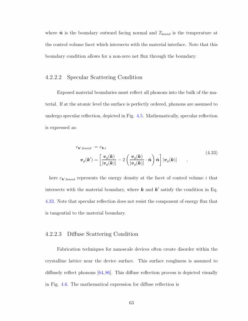
where n is the boundary outward facing normal and Tbound is the temperature at
the control volume facet which intersects with the material interface. Note that this
boundary condition allows for a non-zero net flux through the boundary.
4.2.2.2 Specular Scattering Condition
Exposed material boundaries must reflect all phonons into the bulk of the ma-
terial. If at the atomic level the surface is perfectly ordered, phonons are assumed to
undergo specular reflection, depicted in Fig. 4.5. Mathematically, specular reflection
is expressed as:
ek′,bound = ek,i
vg(k′) =
[vg(k)
|vg(k)|− 2
(vg(k)
|vg(k)|· n)
n
]
|vg(k)| ,
(4.33)
here ek′,bound represents the energy density at the facet of control volume i that
intersects with the material boundary, where k and k′ satisfy the condition in Eq.
4.33. Note that specular reflection does not resist the component of energy flux that
is tangential to the material boundary.
4.2.2.3 Diffuse Scattering Condition
Fabrication techniques for nanoscale devices often create disorder within the
crystalline lattice near the device surface. This surface roughness is assumed to
diffusely reflect phonons [64, 86]. This diffuse reflection process is depicted visually
in Fig. 4.6. The mathematical expression for diffuse reflection is
63

vg,i
n
vg,r = vg,i − 2(vg,i · n)
: Bulk Material: Material Boundary
Figure 4.5: Phonon wavepacket undergoing specular reflection
vg,i
n : Bulk Material: Material Boundary
Figure 4.6: Phonon wavepacket undergoing diffuse reflection
ek,bound =1
N
∑
k′
ek′,i ; vg(k′) · n > 0
N =∑
k′
1 such that vg(k′) · n < 0 ,
(4.34)
64

here ek,bound is the same expression as in Sec. 4.2.2.2. Diffuse scattering serves to
redistribute energy incident on the boundary isotropically. Note that diffuse scat-
tering does resist the component of energy flux tangential to the material boundary,
thus diffuse scattering engenders thermal resistance.
All three types of boundary conditions amount to specifying the solution vari-
able ek,i and are therefore essential or Dirichlet boundary conditions. Additionally,
diffuse and specular boundary conditions are dependent upon the prevailing en-
ergy field and will therefore require iteration to obtain the appropriate steady state
solution.
4.2.3 Computational Implementation
The final portion of this section covers the specifics of implementing the nu-
merical algorithm detailed in this chapter into a Boltzmann transport equation
code. A primary function of the code is to assemble and solve the linear system
(terms given by Eqs. 4.23 and 4.24) for each allowed wavevector and branch. There
exist a wide array of linear solver packages capable of solving the linear system.
In choosing which linear solver package to implement three criterion were consid-
ered. First the linear solver needed to use condensed row storage (CRS) in order
to avoid unnecessary floating point operations that grow costly for simulation of
large systems. Additionally, the solver must be capable of inverting non-symmetric
matrices, such as those that arise through application of the upwinding condition.
65

Finally the solver must be iterative in nature as direct methods would again prove
too computationally expensive for large systems.
A generalized minimum residual (GMRES) iterative solver satisfying the three
criterion was chosen as it provided a combination of speed and accuracy. Specifics of
the solver implementation are as follows: the matrices are preconditioned through
an incomplete LU preconditioning step, twenty Krylov subspaces were used in the
inversion, and eight orders of magnitude reduction in the residual was enforced as a
convergence criterion. The GMRES solver as well as the preconditioner routine are
provided through the open source sparse matrix computation tool kit, SPARSKIT
[87]. Implementation of this linear solver gave a 40 times speed up for a problem size
of 1000 control volumes when compared to a direct solver which stores the entire
linear system.
In Sec. 4.2.2 it was mentioned that due to the nature of specular and diffuse
boundary conditions, the steady state solution must be computed iteratively. As
a result a condition must be established to determine when the numerical solution
e(k)i : i ∈ (1, · · · , NCV ) is sufficiently ”close” to the exact solution e(exact)
i : i ∈
(1, · · · , NCV ). Since the exact solution is in general not known, an alternative
metric for determining convergence is required. This is done by taking the l2 norm
of the difference of the total system energy vector for consecutive iterations and
requiring that it be sufficiently small with respect to the initial difference between
iterations one and two. Mathematically this condition is stated as,
‖e(k) − e(k−1)‖2 < ǫ ‖e(2) − e(1)‖2 (4.35)
66

where the l2 norm has the traditional definition:
‖v‖2 =[
N∑
i
v2i
]1/2
v ∈ RN . (4.36)
The value of ǫ is dependent on the desired accuracy of the final solution and is
generally in the range 10−4 to 10−10.
The algorithm detailed in this section involves solution of the Boltzmann trans-
port equation for all allowable wavelengths and branches within the anisotropic first
Brillouin Zone. While this approach is more rigorous than gray or isotropic assump-
tions, it becomes computationally expensive for large system sizes. In Sec. 3.5 it
was shown that the finite size of a system restricts the allowed wavevectors within
the Brillouin zone. In addition the number of these allowed wavevectors increases
proportional to the volume of the crystal. Therefore within this algorithm, a lin-
ear system must be constructed and inverted for every allowed wavevector and all
branches, which is a computationally demanding procedure. However, for a given
iteration n, the assembly and solution of the linear system for a wavevector k is
dependent only on prevailing values of the temperature and energy field, geometric
quantities specific to the mesh, and phonon properties calculated a priori to the
simulation. Thus the energy values for each wavevector may be solved for indepen-
dently, allowing for parallelization of the algorithm.
The core concept of parallelization is that certain portions of a computer code
may be shared between separate computing threads. These threads then perform
operations simultaneously before returning control to a master thread which then
67

moves on to the next portion of the computer code, this process is depicted in
Fig. 4.7. Parallelization is implemented within the Boltzmann transport equation
Serial Region
Parallel Region
Serial Region
Thread
0
Thread
0
Thread
1
Thread
2
Thread
3
Thread
n
Thread
0
Figure 4.7: A computer code with serial and parallel regions. A master thread(Thread 0) controls program flow within a serial region. When a parallel regionis encountered work is distributed to n threads. Upon completion of the parallelregion control is returned to the master thread.
code via OpenMP directives. OpenMP is a computing tool comprised of compiler
directives, library routines, and environment variables for use on shared-memory
68

machines [88]. By assembling and solving linear systems in parallel a 20 times speed
up is achieved when using 40 threads with a system size of 1000 control volumes.
A flow chart detailing the numerical algorithm outlined in this chapter for
solving the Boltzmann transport equation is given in Fig. 4.8. Thus determination of
the temperature profile through the Boltzmann algorithm may now be summarized:
69

Determine phonon inputs:
• frequencies (ω)
• group velocity (vg)
• specific heat (CV )
• relaxation time (τ)
Define problem set up:
• material dimensions
• spatial mesh
Initialize Temperature
• Ti = Tinit
Initialize Energy (Eq. 4.35)
• ek,i = CV,k × (Ti − Tref)
Calculate boundary conditions from prevailingenergy and temperature field (Eqs. 4.32, 4.33, 4.34)
Assemble linear system Kkek = fkfor phonon mode (k, λ)(Eqs. 4.23 and 4.24)
Solve for solution variable ek
Have all wavevectors k and branches been solved for?
Select newphonon mode
(k, λ)
Sum all wavevectors to get energy field (Eq. 4.25)
Update temperature field (Eq. 4.30)
Has the solution solution varibale converged? (Eq. 4.35)
Proceed tonext iterationselect phononmode (k, λ)
Print energy and temperature fields
no
yes
no
yes
Solver Region
Iterative Region
Figure 4.8: Control flow within Boltzmann transport code.
70

The fundamental difference between the algorithm presented in this chapter
and those presented in the literature is the solution of the Boltzmann transport
equation for all allowed wavevectors and branches within the anisotropic Brillouin
Zone. By solving the Boltzmann transport equation for every allowed wavevec-
tors and branches, anisotropy in the phonon transport may be captured in three
dimensional nanoscale simulations.
In this section a method of solving the Boltzmann transport equations has
been presented. The algorithm requires phonon properties as well as material di-
mensions as inputs and then solves the Boltzmann transport equation for all allowed
wavevectors and all branches in a three-dimensional domain. It is this solution tech-
nique which accounts for all vibrational modes, and thus all energy carriers, that
leads to a more fundamental model than what has previously been presented in the
literature. This capability coupled with the multi-dimensionality of the numerical
procedure generates a Boltzmann transport code capable of capturing the wide ar-
ray of phonon physics that occur within a nanoscale device. In the next section the
code’s capabilities are demonstrated. First a simulation of semi-ballistic transport
is performed and results obtained from the BTE code are compared to the semi-
analytical solutions to verify the mathematical accuracy of the code. Next a study is
performed to compare BTE solutions obtained under the isotropic solution to BTE
solutions which account for full Brillouin zone anisotropy. Finally a FinFET device
parameter study is performed to showcase the three-dimensional capability of the
solver.
71

Chapter 5: Simulations and Results
5.1 Semi-Ballistic Transport
The Boltzmann transport equation is capable of accurate thermal modeling
in regimes where phonon transport is dominated by boundary scattering, such as
on the nanoscale. Accurate thermal modeling at the nanoscale requires capturing
transport from the ballistic regime, where phonons propagate without scattering
with other carriers, to the diffusive regime, where phonon-phonon scattering dom-
inates, this range of transport is referred to as semi-ballistic transport. Methods
such the Fourier equation of heat transfer assume that transport is completely dif-
fusive and are therefore only valid within the diffusive regime. Thus a simulation
of semi-ballistic transport may serve as a verification problem, testing the capabil-
ity of the BTE code to accurately model transport spanning diffusive to ballistic
regimes. Semi-analytical solutions of semi-ballistic transport are available within
the radiative transport literature, one such example is the plane-parallel problem.
The plane-parallel problem determines the radiation intensity field in a one dimen-
sional domain with absorbing and emitting gray media. Solutions to such a problem
have long been studied in the radiation transport literature [89–91]. The physics of
radiative transport are very similar to phonon transport, where instead of quantized
72

lattice vibrations, quantized electromagnetic waves carry energy. In this section, the
problem set up for the plane-parallel problem is detailed, the analytical expression
for the exact solution is given along with the solution method, finally the results ob-
tained from the Boltzmann transport equation solver are verified against the exact
solution.
5.1.1 Verification Problem Set-Up
The physical setup of the plane-parallel problem is depicted in Fig. 5.1, note
that the wall temperature slip is characteristic of semi-ballistic transport, where the
temperature slip, ∆T , becomes zero in the diffuse transport limit. The governing
differential equation for the radiative intensity field in such a problem may be written
as [90]:
s · ∇I = β (Ib − I) , I = I(r, s)
I(0, s) = Ib(T1) ; s · x > 0
I(τL, s) = Ib(T2) ; s · x < 0
(5.1)
where s represents the propagation direction, I the radiative intensity, and Ib the
blackbody equilibrium intensity. The quantity τL is the optical thickness of the
problem and is a measure of how strongly the radiative field interacts with the
medium. The analogous quantity, to τL in phonon physics is the Knudsen number
(Kn) which is defined as Kn = Λ/L, where Λ is the mean free path (MFP) and L
is the length of the domain. The MFP for a given wavevector k is Λk = |vg(k)|τk,
therefore each phonon mode will have its own Kn. For the remainder of of the
73

T1
T2
T
x
∆T
: Temperature Profile
Figure 5.1: Temperature profile of a gray absorbing-emitting medium between twoinfinite parallel plates at temperature T1 (red) and T2 (blue). The temperatureprofile displays a temperature slip ∆T at the boundaries, a characteristic of semi-ballistic transport
section we will work with a single averaged phonon mode and thus Kn will have
a single unique value. A Kn ≪ 1 correspond to diffusive transport, while a Kn
≫ 1 corresponds to the ballistic regime. It is important not to confuse the τk, the
phonon relaxation time, with τL, the optical thickness for radiation transport.
74

The general solution for the non-dimensional temperature field in an absorbing-
emitting gray medium is given by [90]:
Φb(τ) =1
2
[
E2(τ) +
∫ τL
0
Φb(τ′)E1 (|τ − τ ′|) dτ ′
]
Φb(τ) =T 4(τ)− T 4
2
T 41 − T 4
2
,
(5.2)
where the elliptic integral is defined as:
En(x) =
∫ 1
0
µn−2e− x/µdµ . (5.3)
Integral Equations of this form may be solved through the method of successive
approximations, where an initial guess of the desired function, Φkb is substituted into
the RHS of Eq. 5.2, the RHS of Eq. 5.2 is then computed yielding an updated,
Φk+1b , the resulting function is then used as the guess in the k + 1 iteration. This
procedure is outlined in Fig. 5.2. Using the method of successive approximations
in conjunction with numerical quadrature, Φb was computed numerically for use in
verification of the Boltzmann algorithm.
To compare to the numerical solution, the inputs to the BTE code must be
altered to simulate gray photon transport. To that end a spherical Brillouin zone
is created to simulate the isotropic continuum of propagation directions allowed for
photons in radiative transport, see Fig. 5.3. As the the system being modeled
is gray, i.e. frequency independent, all phonon properties are assumed constant
75

Rewrite Integral Equation in iterative form :
Φb(τ) =12E2(τ) +
12
∫ τL0
Φb(τ′)E1(|τ − τ ′|)dτ ′
↓
Φn+1b (τ) = 1
2E2(τ) +
12
∫ τL0
Φnb (τ
′)E1(|τ − τ ′|)dτ ′
Make initial guess for Φn=0b :
Φ0b(τ) =
12E2(τ)
Calculate Φn+1b from Φn
b :
Φn+1b (τ) = 1
2E2(τ) +
12
∫ τL0
Φnb (τ
′)E1(|τ − τ ′|)dτ ′
Compare change, δ in Φb from succesive iterations :
δ = ||Φn+1b − Φn
b ||2
Is δ less thansome predetermined
tolerance, i.eδ < ǫ ?
Set Φnb = Φn+1
b
and performanother iteration
Convergence reached :
Φnb = Φb
yes
no
Figure 5.2: Method of successive approximations approach to solving the integralequation for the exact solution to the plane parallel problem
76

Figure 5.3: Schematic of a spherical Brillouin Zone.
except for the group velocity which was assumed to be constant in magnitude, and
collinear with the wavevector. The gray phonon properties are given in Table 5.1.
The simulation domain geometry replicates infinite parallel plates by specifying the y
and z dimensions to be many orders of magnitude larger than the x dimensions. The
plate at the x = 0 boundary was specified to be a Fourier interface condition with
T1 = 301 K and the high x boundary was specified to be a Fourier interface condition
T2 = 300 K. These conditions are analogous to the blackbody emitter-absorbers
from the plane parallel problem. The distance between the plates was varied to
investigate several Knudsen numbers (i.e. transport regimes). The transport regime
is quantified by the Knudsen number where as the separation goes to zero (Kn ≫ 1)
77

Specific Heat 1.631× 10⁶ Jm3·sec
Group Velocity Magnitude 6400 msec
Relaxation Time 7.2× 10⁻¹² sec
Frequency 16.0 THz
Mean Free Path 4.608× 10⁻⁸ m
Table 5.1: Gray phonon properties
transport becomes ballistic, and as the separation reaches several mean free paths
(Kn < 1) the transport becomes more diffusive.
5.1.2 Verification Results
The results of the simulations for a range of Knudsen numbers are plotted in
Figs. 5.4, 5.5, 5.6, and 5.7.
78

0 0.05Λ 0.1Λ300
300.2
300.4
300.6
300.8
301
x
T
Temperature vs. Distance (Kn = 10)
Numerical SolutionBTE Algorithm Solution
Figure 5.4: Temperature profile for domain length of 110
Λ
0 0.25Λ 0.5Λ300
300.2
300.4
300.6
300.8
301
x
T
Temperature vs. Distance (Kn = 2)
Numerical SolutionBTE Algorithm Solution
Figure 5.5: Temperature profile for domain length of 12Λ
79

0 0.5Λ 1.0Λ300
300.2
300.4
300.6
300.8
301
x
T
Temperature vs. Distance (Kn = 1)
Numerical SolutionBTE Algorithm Solution
Figure 5.6: Temperature profile for domain length of 1 Λ
0 1.0Λ 2.0Λ300
300.2
300.4
300.6
300.8
301
x
T
Temperature vs. Distance (Kn = 1/2)
Numerical SolutionBTE Algorithm Solution
Figure 5.7: Temperature profile for domain length of 2 Λ
For all transport regimes the agreement is excellent between the numerical
algorithm and the exact solution.
80

In addition to verifying the Boltzmann algorithm over a range of transport
regimes, a mesh convergence study was performed to ensure that the algorithm
converges to the exact solution as the mesh is refined. The results of the mesh con-
vergence study, Fig. 5.8, give confidence that the algorithm has been implemented
into the BTE code in a manner which reproduces exact numerical solutions.
101 102
10−4
10−3
10−2
Error =.014N−1.06
Number Control Volumes(N)
RMSError
Root Mean Square Error in Disrete Brillouin Zone Algorithm
Line of Best FitRMS Error
Figure 5.8: Logarithmic plot of root mean square (RMS) error between the Boltz-mann algorithm and the exact numerical solution from [90]. Kn = 10.
81

The BTE code results for the semi-ballistic transport simulations have been
compared to semi-analytical solutions from radiation transport. The excellent agree-
ment verifies that the BTE algorithm has been correctly implemented into a BTE
code. In the following section the code is used to investigate the effect of Bril-
louin zone anisotropy. Finally the code is used to perform a parameter study of a
nanoscale device.
5.2 Effect of Anisotropy
The vast majority of studies which use the Boltzmann transport equation
to model nanoscale heat transport assume that high symmetry phonon properties
prevail in all directions within the Brillouin zone. This assumption is equivalent to
obtaining the dispersion curves of some material along a single high symmetry line,
most often along the Γ−X high symmetry line for the case of silicon( see Fig. 5.9),
and assuming those frequency values are isotropic throughout a spherical Brillouin
zone. Therefore, at any point in the Brillouin zone the frequency at that location is
a function of |k| only, as the frequency is assumed spherically symmetric.
The consequence of these assumptions is twofold. First, the assumption effec-
tively reduces the Brillouin zone shape to that of a sphere, as opposed to its true
shape of a truncated octahedron for an FCC crystal (inset of Fig. 5.9). Within this
sphere the frequencies, and all frequency dependent properties such as specific heat,
are assumed to be distributed isotropically. Secondly, the group velocities become
collinear with the wavevector and are therefore always directed radially outward.
82

Γ X
ω
Dispersion Curve in Silicon along [100] Direction
Figure 5.9: Vibrational frequencies in silicon along the high symmetry line Γ − Xcorresponding to the [100] direction. The inset depicts the Γ−X line (thick blackline connecting the blue dots) within the first Brillouin zone of silicon
The true behavior of phonons within the anisotropic Brillouin zone is in fact-
more complex. Consider the constant frequency contours of various branches within
the kz = 0 plane of the true anisotropic Brillouin zone given in Fig. 5.10. If the
the Brillouin zone plane were isotropic these contours should be circular. However,
only in certain regions can the contours be approximated as circles. The top row
of Fig. 5.10 corresponds to the acoustic modes which are believed to dominate
heat transport. The longitudinal acoustic mode (top right) is roughly circular near
the Brillouin zone plane center, however the contours deviate strongly away from
83

Figure 5.10: Frequency contours within the kz = 0 first Brillouin zone for the firsttransverse acoustic branch (top left), the longitudinal acoustic branch (top right),the first transverse optical branch (bottom left), and the longitudinal optical branch(bottom right).
circular near the Brillouin zone edge, becoming more square-like. The transverse
acoustic mode (top left) remains roughly square throughout the Brillouin zone plane
suggesting that the assumption of an isotropic Brillouin zone could lead to errors
in the phonon properties supplied to the Boltzmann transport equation. To verify
whether frequency values are truly anisotropic in three dimensions a fine grid of
wavevectors was created and the frequency values were determined via molecular
84

dynamics. The resulting frequency space was then discretized and all wavevectors
corresponding to a frequency falling within a certain interval of frequency space were
plotted. It was found that the constant frequency surface of the transverse acoustic
mode is in fact a cube in three dimensions, see Fig. 5.11, further disproving the
isotropic assumption.
Figure 5.11: Constant frequency wavevectors of the transverse acoustic branch. Theblue edges of the constant frequency square are visual guides
.
85

The anisotropy of frequencies within the Brillouin zone affects the phonon
group velocities. In the isotropic assumption the group velocities, defined as vg =
∇k ω, are directed radially away from the Brillouin zone origin. However, it is shown
in Fig. 5.12 that this simplification is not realistic. Figure 5.12 shows that away from
the Brillouin zone center, frequencies become more anisotropic and the direction of
phonon propagation deviates strongly from the radial direction. Additionally, for
the transverse acoustic mode the majority of phonon propagation directions align
along the x, y, z Cartesian directions, while a smaller percentage lie along the
diagonal directions. Since the phonon group velocity is the speed and direction
in which energy of a given mode is carried, therefore advection of a phonon mode
will strongly depend on group velocity. Therefore, Fig. 5.12 would suggest that
advection will be largest along the x and y directions and reach a minimal value
along the diagonal directions.
The anisotropic distribution of frequency in the Brillouin zone, along with
phonon mode group velocities which deviate from the radially outward direction,
indicate that temperature profiles obtained using the isotropic assumption may incur
some error. A two dimensional simulation of a thin silicon film with a heat source
was performed to study what effect, if any, anisotropy has on phonon transport and
the resulting temperature profile. The dimensions of the heat transport problem are
given in Fig. 5.13, in addition the thickness of the film was set to 17.4 nanometers
with diffusely reflecting boundary conditions.
Note that in general, different forms of the Boltzmann transport equation
(i.e. gray, frequency dependent with isotropic assumption, or fully anisotropic)
86

Figure 5.12: Constant frequency wavevectors of the transverse acoustic branch. Thearrows protruding from each wavevector indicate the direction of phonon propaga-tion in the kz = 0 plane
.
will predict different peak temperatures in the simulation of a heated domain [19].
Therefore comparison of the absolute temperature profiles of two different models
may not reveal the variation in heat conduction along different directions in the
plane. However, this study focuses on whether or not phonon properties, and group
velocities, obtained along a single high-symmetry line, are a valid description of heat
87

heated region
100K Fourier boundary
100K Fourier boundary
100 nm
100 nm
20 nm
S = 1016 J/m3s
Figure 5.13: Simulation domain for the study of anisotropic effects in a thin siliconfilm.
transport along all directions. In order to study this assumption, the temperature
profiles of two different Boltzmann transport models should be normalized so that
the maximum temperature for each model is equal. For simplicity the following
normalization is used,
Tnormalized =T − Tmin
Tmax − TminTmin = 100K . (5.4)
The effect of this normalization is to restrict the temperatures within the domain to
be between 0 and 1. Throughout the rest of this section any reference to temperature
will implicitly be referring to the normalized temperature.
88

A reference isotropic solution was required for comparison to the anisotropic
result. Therefore, a gray isotropic phonon simulation was performed to discretize
and solve the Boltzmann transport equation. The spatial domain was discretized
into a 71 × 71 grid of control volumes. The source term in the heated region is
distributed equally into all phonon modes. The phonon properties for this simulation
are identical to those used in the verification problem, which were given in Table
5.1. Due to the symmetry of the problem only a quarter of the plate was actually
simulated, the constant temperature contours of the isotropic simulation are given
in Fig. 5.14.
An anisotropic simulation was subsequently performed. All material and
phonon properties of silicon were obtained from the molecular dynamics approach
detailed in Sec. 4.1. The relaxation time model used was detailed in Sec. 4.1.2.
Since the purpose of this study is to investigate the directional dependence of heat
transport, only acoustic phonon modes were included in the simulation. The same
spatial mesh that was used in the isotropic simulation is used in the anisotropic
case. The source term was again equally distributed amongst all phonon modes.
The constant temperature contours for the anisotropic simulation are given in Fig.
5.15. Note the flattening of the temperature contours along the diagonal direction,
this flattening is most evident for the .3 temperature contours.
In order to directly compare the isotropic simulation to the anisotropic sim-
ulation, the difference between the two temperature profiles was taken. To obtain
the difference in the temperature profiles, the cell centered temperature values of
the anisotropic simulation were subtracted from the cell centered temperatures of
89

.9
.8
.7
.6
.5
.4
.3
.2
.1
x (nm)
y(nm)
Figure 5.14: Constant temperature contours obtained through solving the grayisotropic Boltzmann transport equation
the isotropic simulation,
Tdiff = Tisotropic − Tanisotropic . (5.5)
The contours of the temperature difference of the two simulations are given in Fig.
5.16, in addition the percent differences between the two simulations are given in
5.17.
90

.9
.8
.7
.6.5
.4
.3
.2
.1
x (nm)
y(nm)
Figure 5.15: Constant temperature contours obtained through solving the fullyanisotropic Boltzmann transport equation
The difference in the two solutions reveals that the isotropic assumption does
lead to error in determining the temperature profiles. Furthermore this error is
largest along the diagonal direction. This can be explained by considering the
frequency and group velocity behavior within the Brillouin zone (Figures 5.10, 5.11,
and 5.12). These figures demonstrate that the transverse acoustic modes preferably
transport energy along the ±x or ±y directions as opposed to along any direction.
91

.04436
.03791
.03147
.02502
.01857
.012122
x (nm)
y(nm)
Tdiff =
Tiso−Taniso
Figure 5.16: Constant temperature difference contours obtained by subtracting theanisotropic cell centered temperatures from the isotropic cell centered temperatures.
Therefore, by assuming that transport along the ±x or ±y direction is the same as
along the plate diagonal, as is done within the isotropic assumption, the advection
along the diagonal is exaggerated. This leads to an over prediction of temperatures
along this diagonal line as seen in the temperature difference contours.
Note that the largest temperature difference occurs at 40.833 nanometers from
the origin and 20.833 nanometers from the source term boundary. The majority of
92

2%
4%
6%
8%
10%
12%
14%
16%
x (nm)
y(nm)
Tdiff =
Tiso−TanisoTaniso
Figure 5.17: Percent difference contours between the isotropic and anisotropic sim-ulations.
longitudinal and transverse acoustic phonons will traverse this distance ballistically
without experiencing phonon-phonon scattering. Therefore the isotropic assumption
introduces artificial advection in certain directions. The difference between the two
models is least along the ±x or ±y direction as these directions correspond to the
direction in which the majority of transverse acoustic phonon modes propagate, see
Fig. 5.12. Finally note that at distances far from the source the two models agree
93

closely. This is a result of transport transitioning from ballistic to more diffusive
at these distances. At large distance, transport is dominated by diffusion, resulting
from the relaxation time term, as opposed to advection which is not accurately
modeled through the isotropic model. Therefore the isotropic assumption differs
the most from a fully anisotropic solution in regions where transport is dominated
by advection.
From the results presented in this section it appears that use of the isotropic
assumption may not be valid for two dimensional phonon transport simulations. The
cause for the inaccuracy, which arises from the isotropic assumption, stems from the
anisotropy of frequencies within the Brillouin zone. As a result of this anisotropy, the
group velocities, determined by the frequency values, advect phonons preferentially
along certain directions, leading to an anisotropy in phonon transport.
5.3 FinFET Design and Self-Heating
The Boltzmann transport equation algorithm presented in this work, is ca-
pable of modeling nanoscale heat flow in three dimensions. This capability has
application in the simulation of field effect transistors with a three dimensional fin
geometry (FinFET). The benefit of modeling the temperature profile in a transistor
is two fold. First it is important to determine the maximum temperature within a
transistor as critical electronic properties of the transistor are negatively affected by
temperature. These electronic properties include the drain saturation current and
the threshold voltage [11]. Sufficiently large temperatures reduce saturation current
94

and threshold voltage, effectively reducing the transistor lifetime [11]. Therefore
thermal profile information is critical in determining possible failure in such devices
as well as predicting the long term reliability of the transistor device. The useful-
ness of the simulation is enhanced by the fact that experimental measurements of
transistors are difficult to perform due to the nanometer length scales of current
transistor designs. The second benefit of nanoscale modeling lies in the profiling of
new transistor designs. A wide array of device geometry parameters may be varied
and the temperature profile within the device may be modeled using the presented
algorithm to determine the design which most efficiently dissipates heat. The set
of geometric parameters which yield the lowest peak hotspot temperature should
maximize device performance and lifetime.
5.3.1 Problem Set-Up
A parameter study of a silicon on insulator (SOI) fin field effect transistor
(FinFET) was performed with the goal of analyzing the effect of fin width, and
source region geometry, on the peak temperature obtained within the fin. Three fin
widths were chosen as well as three source region geometries. In order to allow for
comparison between the various parameter combinations the overall energy sourced
into each FinFET is maintained at a constant value. The parameter values for
the FinFET and source region were drawn from the literature to ensure that the
simulations reflect realistic physical conditions of FinFET transistor devices. The
FinFET device has a characteristic length scale of ten nanometers, reducing the
95

ΓX
M R
(a) (b)
Figure 5.18: Idealized Simple Cubic Lattice: (a) Brillouin Zone including high sym-metry points (Γ, X , M , and R) and lines (dotted), (b) real space lattice primitiveunit cell with atoms at vertices.
number of allowed vibrational modes as compared to a bulk device. In addition the
FinFET length scales are on the same order of magnitude as the phonon MFP’s
placing transport within the fin in the semi-ballistic regime. The device geometry,
source terms, and boundary conditions all vary in three dimensions, resulting in
three dimensional temperature profiles. Therefore, the wide array of features within
the presented Boltzmann algorithm are required for accurate modeling of the SOI
FinFET device.
For simplicity, it was assumed that the FinFET is composed of an idealized
Lennard-Jones solid with a simple cubic crystal lattice, the real space unit cell as
well as the associated Brillouin zone of the material are depicted in Fig. 5.18. The
chosen interatomic potential is the Lennard-Jones potential which has the form:
VLJ,n(rij) = 4Bn
(A12
n
r12ij− A6
n
r6ij
)
; n = NN or NNN ,
96

here rij is the distance between atom i and atoms j, An and Bn are constants chosen
to reproduce the lattice constant and frequency spectrum displayed by common
semiconductor materials, and NN and NNN represent the interactions between
nearest neighbor and next-nearest neighbor respectively. The constants appearing
in the interatomic potential are given in Table 5.2.
Empirical Potential Constants
Ann 4.4545× 10⁻¹⁰ meters
Bnn 2.7× 10⁻²⁰ Joules
Annn 6.2996× 10⁻¹⁰ meters
Bnnn 1.9× 10⁻²⁰ Joules
Table 5.2: Lennard Jones parameters
The phonon properties are determined from the analytical form of the inter-
atomic potential, using the methods detailed in Sec. 3.3 and 4.1. The resulting
dispersion along the high symmetry lines of the cubic Brillouin zone are given in
Fig. 5.19. From the dispersion relations, the phonon group velocities are obtained
through the central differencing procedure outlined in Sec. 4.1.
The phonon relaxation times are obtained from literature values given in
ref. [1]. This relaxation time model was chosen as it accounts for the temperature
and frequency dependence of relaxation times. In addition the model differentiates
between both longitudinal and transverse modes as well as between normal and
97

Γ X M Γ R
·104
ω
Dispersion Relations in High-Symmetry Directions
Figure 5.19: Frequency - wavevector relations for a series of high-symmetry lineswithin the first Brillouin zone
Umklapp scattering processes. Finally, the functional forms have been fit to exper-
imental data and accurately reproduce the thermal conductivity values in semicon-
ducting materials [1]. The functional forms of the various phonon scattering rates,
along with the parameter values, are reproduced from [1] in Tables 5.3 and 5.4.
A source term is incorporated into the appropriate BTE’s in order to model
electron - phonon interactions or Joule heating. Joule heating occurs when high
energy electrons interact with the lattice, transferring their energy to the lattice and
creating phonons. The vast majority of electron-phonon interaction occurs within
a region of the transistor known as the channel [9]. The location of this channel
region is assumed to coincide with the fin region of highest electron density. Due
to the high energy of electrons within the channel, the majority of energy is known
to be transferred to high frequency phonons [9]. In order to capture this effect, a
98

Phonon Branch UmklappScatteringRate (τ−1
U )
NormalScatteringRate (τ−1
L )
Transverse BTUω2Te−CT/T BTωT
4
Longitudinal BLUω2Te−CL/T BLω
2T 3
Table 5.3: Functional form of the phonon scatter-ing rates from [1]
Scattering Rate Parameters
BT (K−4) 2× 10⁻¹³
BTL (s/K−3) 2× 10⁻²¹
BTU (s) 1× 10⁻¹⁹
BLU (s) 5× 10⁻¹⁹
CT (K) 55
CL (K) 180
Table 5.4: Parameter values for phonon scatteringrates in Table 5.3 given by [1]
source term is included in the BTE’s (i.e. Sk 6= 0 in Eq. 4.31) corresponding to
phonon states which have a frequency ω(k) ≥ ωmax/2 where ωmax is the maximum
vibrational frequency of the material. As a result of this assumption, energy is
injected into high frequency modes which tend to have lower group velocity and are
thus inefficient at transporting thermal energy. Therefore the removal of heat will
require energy to decay from high frequency modes to lower frequency modes which
then carry the heat away from the heated region.
Joule heating occurs in the regions of the transistor with high electron density,
i.e. the channel. Electron density may be determined through solving the problem of
electron transport, this is typically done using the Monte Carlo method to solve the
99

Boltzmann transport equation for electrons [56]. The electron density for the device
considered in this study is found to vary with the applied gate voltage [3], where as
the gate voltage is increased, electrons are pulled toward the gate interface at the
corners of the device, see Fig. 5.20. To capture this variation, the parameter study
Figure 5.20: Evolution of carrier concentration with applied gate voltage, figureobtained from [3]
considers three different configurations of the source region. These configurations
are meant to reflect the location and size of the channel for a range of applied
voltages, these regions are depicted in Fig. 5.21. The source is applied in such a
manner that the energy injected into the channel is constant for all fin widths and
for all channel geometries (the three regions are henceforth referred to as channel
100

25 nm
8 nm
8.33nm
2.66nm
8.33nm
2nm
0.66nm
4.16nm
Channel 1 Channel 2 Channel 3x
y
Figure 5.21: Three channel geometries simulated in FinFET device. Channel Icorresponds to low applied gate voltage, channel II corresponds to medium appliedgate voltage, and channel III corresponds to high applied gate voltage.
I, channel II, and channel III). The depth (in the x-direction, i.e. into the page)
of all channels is set to 10 nanometers, this value was found to be the length of
the channel from Monte Carlo simulations of electron-phonon coupling [8]. The
simulation domain dimensions are varied to investigate the effect of fin width on the
temperature profile within a FinFET. Three simulation domains were considered,
depicted in Fig. 5.3.1. The geometries of the devices being simulated are drawn
from [3] and reflect current FinFET transistor device design.
Due to symmetry in the x and y directions only a quarter of the FinFET need
be simulated, however the allowed wavevectors must reflect the dimensions of the
full crystal. The quarter domain to be simulated is depicted in Fig. 5.25 along
with the associated boundary conditions. Specular boundary conditions are applied
101

25
8
40
Figure 5.22: Thin Fin
25
40
12
Figure 5.23: Medium Fin
25
40
16
Figure 5.24: Thick Fin
to the symmetry surfaces. Diffuse boundary conditions are applied to the exposed
surfaces of the FinFET as fabrication techniques for these devices cause disorder in
atoms near the surface [92], this disorder results in diffuse phonon scattering at these
boundaries. Finally, Fourier boundary conditions are applied to the silicon/silicon
dioxide interfaces. It is assumed that the majority of heat generated within the
FinFET is removed through these surfaces. All Fourier boundary conditions are set
102

Figure 5.25: Boundary conditions applied to the simulation domain.
to 300 K, where it is the maximum rise in temperature over 300 K that is of the
most importance to the performance of the FinFET.
5.3.2 Device Simulation Results
With the phonon inputs, and physical properties defined, device simulations
were performed for all three channels and all three fin widths, resulting in a total of
nine simulations. The temperature contours of each simulation are grouped based
on the channel region in order to illuminate the effect of fin width (Figs 5.26, 5.27,
and 5.28).
Consider channel I whose temperature contours are given in Fig. 5.26. Be-
gin by noting that the region of maximum temperature occurs in the center of the
103

channel region. Furthermore, the temperatures are highest within the channel and
decrease sharply outside the channel. Both of these effects are a result of energy
being distributed to high frequency modes with low group velocity due to electron-
phonon interactions within the channel. As a result energy is confined to the channel
region before decaying into lower frequency modes with higher group velocity which
are capable of transporting energy out of the domain. Note also the slight temper-
ature rise which occurs in the (+x,+y,+z) region. This is a result of the adiabatic
boundary conditions trapping phonons in the domain, all energy must leave via the
(−y) plane or through the (−z) plane. Finally, it is important to consider the trend
in maximum channel temperature as this will have the largest effect on the electri-
cal performance of the FinFET. The trend observed here is that as the fin width
decreases, the peak temperature increases.
Consider now channel II temperature contours, which are given in Fig. 5.27.
The temperature profile for this channel region is spread over a larger portion of
the domain as a result of spreading of the source term. Recall that this spreading
effect comes from an increase in the applied gate voltage which reduces the spatial
electron density. The temperature profile inside the domain is observed to be less
than for channel I. This reduction is a result of shifting the channel region closer
to the Fourier interface boundary. By moving the channel closer to the Fourier
boundary which allows phonons to flow out of the domain, heat generated in the
high frequency modes with low group velocity can be transported out of the domain
directly. Therefore, the process in which energy must be transferred to lower group
velocity modes (a process which is limited by the mode relaxation times), before
104

X
Y
Z
Temperature
311310309308307306305304303302301
X
Y
Z
Temperature
309308.5308307.5307306.5306305.5305304.5304303.5303302.5302301.5301300.5
X
Y
Z
Temperature
307.5307306.5306305.5305304.5304303.5303302.5302301.5301300.5
Figure 5.26: Temperature profiles for channel 1. All temperatures are reported inunits of Kelvin.
being transported out of the system, is partially circumvented. This more efficient
process of heat removal results in the lower overall temperatures observed in channel
II. Again, note the trapping of energy along the (+x,+z) boundary edge, resulting
from adiabatic boundary conditions. As with channel I, an decrease in fin width
corresponds to an increase in maximum temperature for channel II.
105

X
Y
Z
Temperature
303.6303.4303.2303302.8302.6302.4302.2302301.8301.6301.4301.2301300.8300.6
X
Y
Z
Temperature
302.8302.6302.4302.2302301.8301.6301.4301.2301300.8300.6300.4
X
Y
Z
Temperature
302.4302.2302301.8301.6301.4301.2301300.8300.6300.4
Figure 5.27: Temperature profiles for channel 2. All temperatures are reported inunits of Kelvin.
Finally, consider the channel III temperature contours given in Fig. 5.28.
This channel configuration produces the highest temperatures. These temperature
contours strongly mirror the channel region itself. Channel III lies along a Fourier
interface boundary as does channel II. However, as opposed to channel II, the large
energy generation which exists in channel III cannot be efficiently dissipated by high
frequency phonon modes. This results in channel III displaying the largest overall
106

temperature profiles with respect to the 300 K. Also note the sharp temperature
gradients in regions near the channel. This effect is characteristic of non-equilibrium
ballistic transport at the nanoscale and has been observed in similar device simu-
lations [64]. These sharp temperature gradients are qualitatively different than
those that would be obtained through a classical simulation using Fourier’s equa-
tion of heat transfer. Such a simulation assumes diffusive transport and would yield
smoother temperature gradients. Finally the trend in maximum hotspot tempera-
ture is again that decreasing fin width increases the peak channel temperature.
The central quantity of interest is the maximum temperature rise within the
domain with respect to 300 K. The maximum temperature for all fin widths and
channels is given in Table 5.5. Several conclusions may be drawn from these results.
Thin Fin Medium Fin Thick Fin
Channel 1 312.245 K 309.735 K 308.276 K
Channel 2 303.823 K 303.024 K 302.535 K
Channel 3 324.966 K 319.044 K 316.048 K
Table 5.5: Maximum temperature rise in each simulation.
First, as the channel becomes smaller, corresponding to larger applied gate voltages,
the maximum temperature rise increases. This is to be expected as channel III
corresponds the to the highest electron densities within any channel and therefore
the largest source term. The high source term, in addition to the low group velocity
107

XY
Z
Temperature
324322320318316314312310308306304302
XY
Z
Temperature
318317316315314313312311310309308307306305304303302301
XY
Z
Temperature
315314313312311310309308307306305304303302301
Figure 5.28: Temperature profiles for channel 3. All temperatures are reported inunits of Kelvin.
of phonon modes receiving the energy, lead to large temperature rise of the channel.
Furthermore, a clear trend emerges, for all channels, when considering the variation
of fin width. Namely as the fin width decreases, so does the maximum temperature
achieved in the channel. This effect results from introducing the same amount of
energy into a smaller volume leading to an overall temperature rise.
108

In the final portion of this section the energy density of two particular phonon
modes are visualized, henceforth referred to as mode 1 and mode 2. Tracking the
energy flow within an individual phonon mode represents a capability unique to the
Boltzmann transport equation algorithm presented in this work, whereby individual
mode occupancies may be be examined since the BTE is solved for all allowed
wavevectors and branches within the Brillouin zone. Consider the phonon properties
of mode 1 and mode 2 which are detailed in Table 5.6. The energy density profiles
Mode 1 Mode 2
Frequency (THz) 117.20 7.89
Group Velocity (meters/sec) 0x+ 0y + 0xz −4882.8x+ 1656.37y + 973.58z
Source Term (ω > ωmax/2) Yes No
Relaxation Time (picoseconds) 69.74 28.37
Table 5.6: Phonon properties of two vibrational modes.
of these two modes for channel II in the 8 nm wide fin are detailed in Fig. 5.29.
These modes are chosen to highlight the wide array of phonon physics that manifest
within nanoscale devices for two different modes within the first Brillouin zone.
Analyzing the energy profiles of the two modes, it is clear that the individual
phonon modes may behave in a manner quite different from one another as well as
from the total energy density profile, which is given in Fig. 5.27 (recall that energy
and temperature are proportionally related through the specific heat, this relation
109

X
Y
Z
Phonon Energy Density
100908070605040302010
X
Y
Z
Phonon Energy Density
2.82.62.42.221.81.61.41.210.80.60.40.2
Mode 1 Mode 2
Jm3
Jm3
Figure 5.29: Energy profiles of mode 1 and mode 2. The parameters correspond tothe 8 nm fin width and channel 1 geometry
is given in Eq. 4.30). Considering mode 1 first, note that the shape is identical
to the channel geometry. This is a result of mode 1 having zero group velocity,
therefore none of the energy deposited into this mode can be directly transported.
Rather, energy must decay into other phonon modes through scattering processes,
modeled through the relaxation time term, before being transported. Therefore it
is capacitative modes such as mode 1 that are responsible for the self heating effects
in nanoscale devices.
Mode 2 has an energy profile which is much different from that of the overall
energy density profile, this departure arises from a multitude of factors. First,
mode 2 is of low enough frequency that it does not directly receive energy from
the source term, rather any energy injected into this mode is through phonon-
110

phonon scattering modeled by the relaxation time term or through in-scattering
from boundaries. Furthermore, the region of the material in which the mode is
excited is far removed from the hotspot region, see Fig. 5.27. This separation
arises from energy decaying from capacitative modes, such as mode 1, into lower
frequency (and higher group velocity) modes which then transport energy away from
the domain. When these modes reach the far end of the domain, i.e. the surface
normal to the +x direction, they scatter and diffusely redistribute their energy into
mode 2. Finally it is important to note that mode 2 has a much lower energy
density than mode 1, indicating dominance of the source term over phonon-phonon
scattering when increasing the occupancy of the mode. The dominance of phonon
generation by the source term results in the overall energy density profile more
closely mirroring mode 1, whose BTE contains a source term, over mode 2, whose
BTE does not.
In this section a study of a FinFET device has been performed with the goal
of characterizing the effect of fin geometry as well as source term geometry on the
temperature profiles within the fin. Of specific interest is the peak temperature
achieved, as this has the largest effect on the electronic performance of the FinFET.
It is found that decreasing fin width corresponds to an increase in peak temperature
of the hotspot. Furthermore, the capability of visualizing individual mode occu-
pations was demonstrated by considering two phonon modes with different phonon
properties. Capturing phonon physics of individual phonon modes is an inherent
capability of the presented algorithm, a capability not available the majority of BTE
solvers which appear in the literature.
111

Chapter 6: Conclusion
6.1 Closure
The main goal of this thesis was to solve the fully anisotropic Boltzmann
transport equation for all allowed wavevectors and branches in the first Brillouin zone
and apply this method to nanoscale device simulation. To this end the challenges
inherent in nanoscale thermal modeling were introduced, and a literature review
was presented of previous work that had been performed in the area of nanoscale
thermal modeling. Work done on nanoscale thermal modeling within the framework
of solving the Boltzmann transport equation was highlighted to demonstrate that
the BTE provided accurate description of thermal transport in nanoscale devices.
However, it was noted that many of these works employed simplifying assumptions
which did not fully account for the variation of phonon properties throughout the
anisotropic Brillouin zone.
Following the literature review, the theory behind the physics of phonons was
reviewed. The lattice dynamical approach to obtaining phonon properties was cov-
ered, and the difficulties in accurately described phonon-phonon collisions was dis-
cussed. A relaxation time model was chosen which accurately captured scattering in
thin films. Additionally, the quantum mechanical basis for the particle viewpoint of
112

phonons was introduced to motivate the use of the Boltzmann transport equation.
Finally the notion of discrete allowed wavevectors within the Brillouin zone was
presented. By solving the Boltzmann transport equation for each of these allowed
wavevectors, the anisotropy of phonon properties within the Brillouin zone may be
accounted for.
The algorithm for solving the BTE was given in Sec. 4. The algorithm employs
a control volume discretization to solve the system of differential equations. Phonon
boundary scattering is incorporated by applying specular, diffuse, or Fourier bound-
ary conditions directly to the individual differential equations. Finally, specifics re-
garding the computational implementation were discussed, including parallelization
of the algorithm.
In the results section, the code implementing the BTE algorithm was verified
to ensure mathematical accuracy. The verification problem was borrowed from
radiative transport and described transport in regimes ranging from fully ballistic to
diffusive. Next the validity of the isotropic assumption, which is used in many BTE
models, was tested. Comparison between the anisotropic model used in this work
and the gray isotropic model revealed that the isotropic model may overestimate
advection along certain direction. As a result the temperature profiles obtained from
the two models differ by up to 16 %. Finally a device simulation was performed to
investigate the effects of channel geometry and fin width on the peak temperatures
inside a FinFET transistor. It was found that smaller channels and thicker fins
tended to increase the maximum temperature, while spreading of the channel and
narrowing the fin reduced peak temperatures.
113

6.2 Future Work
The work presented in this thesis represents the first steps towards modeling
phonon transport in three dimensions for a wide variety of devices. Future work, as
well as improvements to the BTE code, include:
(i) Further investigate and quantify the effect of anisotropy. This includes inves-
tigating the effects of anisotropy in all three dimensions as opposed to just two
dimensions. In addition explore materials which display stronger anisotropy
than silicon.
(ii) Implement the time dependent form of the Boltzmann transport equation. The
unsteady form of the BTE will allow for the modeling of transient phenomena
at the nanoscale which cannot be captured in the current BTE code.
(iii) Incorporate the effect of material interfaces into the framework of the BTE
code. In its current state the BTE code is capable of handling only a single
homogeneous material. However modern day nanoscale devices are often het-
erostructures with material interfaces. At such interfaces the effects of phonon
scattering, absorption, and transmission need to be accounted for. Thus simu-
lation of more complex structures will require incorporating material interfaces
into the framework of the existing BTE code.
(iv) The current OpenMP implementation for parallelizing the code should be ex-
tended to MPI parallelization. While the OpenMP parallelization provides a
large reduction in computing time, it is restricted to use on shared memory
114

platforms. Solving the Boltzmann transport equation for all allowed wavevec-
tors, as done in this thesis, is very computationally expensive. Therefore
parallelization through MPI will allow for further performance improvements
that are needed for investigating larger problems.
115

Bibliography
[1] M Asen-Palmer, K Bartkowski, E Gmelin, M Cardona, AP Zhernov, AV In-yushkin, A Taldenkov, VI Ozhogin, Kohei M Itoh, and EE Haller. Thermalconductivity of germanium crystals with different isotopic compositions. Phys-ical review B, 56(15):9431, 1997.
[2] MMKuklja and AB Kunz. Ab initio simulation of defects in energetic materials.part i. molecular vacancy structure in rdx crystal. Journal of Physics andChemistry of Solids, 61(1):35–44, 2000.
[3] Andrew R Brown, Nicolas Daval, Konstantin K Bourdelle, B-Y Nguyen, andAsen Asenov. Comparative simulation analysis of process-induced variabilityin nanoscale soi and bulk trigate finfets. Electron Devices, IEEE Transactionson, 60(11):3611–3617, 2013.
[4] More moore roadmap - itrs 2.0 white paper. Technical report, InternationalTechnology Roadmap for Semiconductors, 2014.
[5] Jeremy Rowlette, Eric Pop, Sanjiv Sinha, Mathew Panzer, and Kenneth Good-son. Thermal phenomena in deeply scaled mosfets. IEDM Tech. Dig, 2005:984–987, 2005.
[6] Eric Pop, Robert Dutton, and Kenneth Goodson. Detailed heat generationsimulations via the monte carlo method. In Simulation of Semiconductor Pro-cesses and Devices, 2003. SISPAD 2003. International Conference on, pages121–124. IEEE, 2003.
[7] Mohamed Mohamed, Zlatan Aksamija, Wolfgang Vitale, Foyzul Hassan,Kyeong-Hyun Park, and Umberto Ravaioli. A conjoined electron and thermaltransport study of thermal degradation induced during normal operation ofmultigate transistors. Electron Devices, IEEE Transactions on, 61(4):976–983,2014.
[8] Eric Pop, Sanjiv Sinha, and Kenneth E Goodson. Heat generation and transportin nanometer-scale transistors. Proceedings of the IEEE, 94(8):1587–1601, 2006.
116

[9] Eric Pop, Robert W Dutton, and Kenneth E Goodson. Monte carlo simu-lation of joule heating in bulk and strained silicon. Applied Physics Letters,86(8):082101, 2005.
[10] Mayank Shrivastava, Manish Agrawal, Sunny Mahajan, Harald Gossner,Thomas Schulz, Dinesh Kumar Sharma, and V Ramgopal Rao. Physical insighttoward heat transport and an improved electrothermal modeling framework forfinfet architectures. Electron Devices, IEEE Transactions on, 59(5):1353–1363,2012.
[11] Yang-Kyu Choi, Daewon Ha, Eric Snow, Jeffrey Bokor, and Tsu-Jae King.Reliability study of cmos finfets. In Electron Devices Meeting, 2003. IEDM’03Technical Digest. IEEE International, pages 7–6. IEEE, 2003.
[12] Per G Sverdrup, Y Sungtaek Ju, and Kenneth E Goodson. Sub-continuumsimulations of heat conduction in silicon-on-insulator transistors. Journal ofHeat Transfer, 123(1):130–137, 2001.
[13] YS Ju and KE Goodson. Phonon scattering in silicon films with thickness oforder 100 nm. Applied Physics Letters, 74(20):3005–3007, 1999.
[14] Baxter H Armstrong. Two-fluid theory of thermal conductivity of dielectriccrystals. Physical Review B, 23(2):883, 1981.
[15] Adam Christensen and Samuel Graham. Multiscale lattice boltzmann modelingof phonon transport in crystalline semiconductor materials. Numerical HeatTransfer, Part B: Fundamentals, 57(2):89–109, 2010.
[16] PG Sverdrup, S Sinha, M Asheghi, S Uma, and KE Goodson. Measurement ofballistic phonon conduction near hotspots in silicon. Applied Physics Letters,78(21):3331–3333, 2001.
[17] Rodrigo A Escobar, Sartaj S Ghai, Myung S Jhon, and Cristina H Amon. Multi-length and time scale thermal transport using the lattice boltzmann methodwith application to electronics cooling. International Journal of Heat and MassTransfer, 49(1):97–107, 2006.
[18] JY Murthy and SR Mathur. An improved computational procedure for sub-micron heat conduction. In ASME 2002 International Mechanical EngineeringCongress and Exposition, pages 75–84. American Society of Mechanical Engi-neers, 2002.
[19] Sreekant V Narumanchi, Jayathi Y Murthy, and Cristina H Amon. Comparisonof different phonon transport models for predicting heat conduction in silicon-on-insulator transistors. Journal of Heat Transfer, 127(7):713–723, 2005.
[20] Sreekant VJ Narumanchi, Jayathi Y Murthy, and Cristina H Amon. Boltz-mann transport equation-based thermal modeling approaches for hotspots inmicroelectronics. Heat and mass transfer, 42(6):478–491, 2006.
117

[21] Eric Pop, Robert W Dutton, and Kenneth E Goodson. Analytic band montecarlo model for electron transport in si including acoustic and optical phonondispersion. Journal of Applied Physics, 96(9):4998–5005, 2004.
[22] David Lacroix, Karl Joulain, and Denis Lemonnier. Monte carlo transientphonon transport in silicon and germanium at nanoscales. Physical Review B,72(6):064305, 2005.
[23] Jean-Philippe M Peraud, Colin D Landon, and Nicolas G Hadjiconstantinou.Monte carlo methods for solving the boltzmann transport equation. AnnualReview of Heat Transfer, 17:205–265, 2014.
[24] Sandip Mazumder and Arunava Majumdar. Monte carlo study of phonon trans-port in solid thin films including dispersion and polarization. Journal of HeatTransfer, 123(4):749–759, 2001.
[25] Syed Ashraf Ali, Gautham Kollu, Sandip Mazumder, P Sadayappan, and ArpitMittal. Large-scale parallel computation of the phonon boltzmann transportequation. International Journal of Thermal Sciences, 86:341–351, 2014.
[26] Daniel P Sellan, JE Turney, Alan JH McGaughey, and Cristina H Amon.Cross-plane phonon transport in thin films. Journal of Applied Physics,108(11):113524, 2010.
[27] X. Huang et al. Sub 50-nm finfet: Pmos. pages 67–70, 445 Hoes Lane, Pis-cataway, NJ 08855, 12 1999. Institute of Electrical and Electronics Engineers,Institute of Electrical and Electronics Engineers.
[28] Joseph E Turney, Alan JH McGaughey, and Cristina H Amon. In-plane phonontransport in thin films. Journal of Applied Physics, 107(2):024317, 2010.
[29] A. R. Brown et al. Comparitive simulation analysis of process-induced vari-ability in nanoscale soi and bulk trigate finfets. IEEE Transactions on ElectronDevices, 60(11):3611–3617, 11 2013.
[30] G.P. Srivastava. The Physics of Phonons. Taylor and Francis Group, 270Madison Avenue New York, NY 10016, 1990.
[31] P Pavone, K Karch, O Schutt, D Strauch, WWindl, P Giannozzi, and S Baroni.Ab initio lattice dynamics of diamond. Physical Review B, 48(5):3156, 1993.
[32] Alistair Ward, DA Broido, Derek A Stewart, and Gernot Deinzer. Ab initiotheory of the lattice thermal conductivity in diamond. Physical Review B,80(12):125203, 2009.
[33] Nicolas Mounet and Nicola Marzari. First-principles determination of the struc-tural, vibrational and thermodynamic properties of diamond, graphite, andderivatives. Physical Review B, 71(20):205214, 2005.
118

[34] A Ward and DA Broido. Intrinsic phonon relaxation times from first-principlesstudies of the thermal conductivities of si and ge. Physical Review B,81(8):085205, 2010.
[35] Stefano Baroni, Stefano De Gironcoli, Andrea Dal Corso, and Paolo Giannozzi.Phonons and related crystal properties from density-functional perturbationtheory. Reviews of Modern Physics, 73(2):515, 2001.
[36] E. Molinari A. Debernardi, S. Baroni. Anharmonic phonon lifetimes in semicon-ductors from density-functional perturbation theory. Physical Review Letters,75(9):1819–1822, 8 1995.
[37] A. Ward and D. A. Broido. Intrinsic phonon relaxation times from first-principles studies of the thermal conductivities of si and ge. Physical ReviewB, 81(8):1–5, 2 2010.
[38] Paolo Giannozzi, Stefano Baroni, Nicola Bonini, Matteo Calandra, RobertoCar, Carlo Cavazzoni, Davide Ceresoli, Guido L Chiarotti, Matteo Cococcioni,Ismaila Dabo, Andrea Dal Corso, Stefano de Gironcoli, Stefano Fabris, GuidoFratesi, Ralph Gebauer, Uwe Gerstmann, Christos Gougoussis, Anton Kokalj,Michele Lazzeri, Layla Martin-Samos, Nicola Marzari, Francesco Mauri, Ric-cardo Mazzarello, Stefano Paolini, Alfredo Pasquarello, Lorenzo Paulatto, CarloSbraccia, Sandro Scandolo, Gabriele Sclauzero, Ari P Seitsonen, AlexanderSmogunov, Paolo Umari, and Renata M Wentzcovitch. Quantum espresso: amodular and open-source software project for quantum simulations of materi-als. Journal of Physics: Condensed Matter, 21(39):395502, 2009.
[39] J-S Wang, Jian Wang, and JT Lu. Quantum thermal transport in nanostruc-tures. The European Physical Journal B, 62(4):381–404, 2008.
[40] Gang Chen. Nanoscale energy transport and conversion. 2005.
[41] JE Turney, ES Landry, AJH McGaughey, and CH Amon. Predicting phononproperties and thermal conductivity from anharmonic lattice dynamics calcu-lations and molecular dynamics simulations. Physical Review B, 79(6):064301,2009.
[42] AJH McGaughey and M Kaviany. Thermal conductivity decomposition andanalysis using molecular dynamics simulations. part i. lennard-jones argon. In-ternational Journal of Heat and Mass Transfer, 47(8):1783–1798, 2004.
[43] Shuze Zhu and Teng Li. Hydrogenation-assisted graphene origami and its ap-plication in programmable molecular mass uptake, storage, and release. ACSnano, 8(3):2864–2872, 2014.
[44] Frank H Stillinger and Thomas A Weber. Computer simulation of local orderin condensed phases of silicon. Physical review B, 31(8):5262, 1985.
119

[45] JG Swadener, MI Baskes, and M Nastasi. Molecular dynamics simulation ofbrittle fracture in silicon. Physical review letters, 89(8):085503, 2002.
[46] Jing Xu, Signe Kjelstrup, and Dick Bedeaux. Molecular dynamics simulations ofa chemical reaction; conditions for local equilibrium in a temperature gradient.Physical Chemistry Chemical Physics, 8(17):2017–2027, 2006.
[47] Peter L Freddolino, Anton S Arkhipov, Steven B Larson, Alexander McPherson,and Klaus Schulten. Molecular dynamics simulations of the complete satellitetobacco mosaic virus. Structure, 14(3):437–449, 2006.
[48] Yongjin Lee and Gyeong S Hwang. Force-matching-based parameterization ofthe stillinger-weber potential for thermal conduction in silicon. Physical ReviewB, 85(12):125204, 2012.
[49] Alan JH McGaughey and Jason M Larkin. Predicting phonon properties fromequilibrium molecular dynamics simulations. Ann. Rev. Heat Transfer, 17:49–87, 2014.
[50] A. J. H McGaughey and M. Kaviany. Phonon transport in molecular dynamicssimulations: Formulation and thermal conductivity prediction.
[51] Alan JH McGaughey and M Kaviany. Quantitative validation of the boltzmanntransport equation phonon thermal conductivity model under the single-moderelaxation time approximation. Physical Review B, 69(9):094303, 2004.
[52] PK Schelling, SR Phillpot, and P Keblinski. Phonon wave-packet dynamics atsemiconductor interfaces by molecular-dynamics simulation. Applied PhysicsLetters, 80(14):2484–2486, 2002.
[53] JE Turney, AJH McGaughey, and CH Amon. Assessing the applicability ofquantum corrections to classical thermal conductivity predictions. PhysicalReview B, 79(22):224305, 2009.
[54] Mehran Kardar. Statistical Physics of Particles, volume 1 of 1, chapter 3, pages57–84. Cambridge University Press, University Printing House, Cambridge CB28BS, United Kingdom, 6 edition, 2007. ””.
[55] Robert E. Peierls. Quantum Theory of Solids. Oxford University Press, AmenHouse, London E.C.4, 1 edition, 1955.
[56] Carlo Jacoboni and Lino Reggiani. The monte carlo method for the solutionof charge transport in semiconductors with applications to covalent materials.Reviews of Modern Physics, 55(3):645, 1983.
[57] JA Fleck and JD Cummings. An implicit monte carlo scheme for calculat-ing time and frequency dependent nonlinear radiation transport. Journal ofComputational Physics, 8(3):313–342, 1971.
120

[58] Ivan Lux and Laszlo Koblinger. Monte Carlo particle transport methods: neu-tron and photon calculations, volume 102. Citeseer, 1991.
[59] Jean-Philippe M Peraud and Nicolas G Hadjiconstantinou. Efficient simula-tion of multidimensional phonon transport using energy-based variance-reducedmonte carlo formulations. Physical Review B, 84(20):205331, 2011.
[60] ASME Majumdar. Microscale heat conduction in dielectric thin films. Journalof Heat Transfer, 115(1):7–16, 1993.
[61] AA Joshi and A Majumdar. Transient ballistic and diffusive phonon heattransport in thin films. Journal of Applied Physics, 74(1):31–39, 1993.
[62] Rodrigo Escobar. Lattice Boltzmann Modeling of Phonon Transport in SiliconFilms. PhD thesis, Carnegie Mellon University, Pittsburgh Pennsylvania, 72005. ””.
[63] Aydin Nabovati, Daniel P Sellan, and Cristina H Amon. On the latticeboltzmann method for phonon transport. Journal of Computational Physics,230(15):5864–5876, 2011.
[64] Syed Ashraf Ali and Sandip Mazumder. Phonon heat conduction in multidi-mensional heterostructures: predictions using the boltzmann transport equa-tion. Journal of Heat Transfer, 137(10):102401, 2015.
[65] C. Kittle. Introduction to Solid State Physics. John Wiley & Sons, Inc., NewYork, 1996.
[66] David J. Griffiths. Introduction to Quantum Mechanics. Pearson Prentice Hall,Upper Saddle River, NJ 07458, 2005.
[67] V. L. Gurevich. Transport in Phonon Systems. North-Holland Physics Pub-lishing, 1000 AC Amsterdam, Netherlands, 1986.
[68] N. W. Ashcroft and N. D Mermin. Solid State Physics. Saunders CollegePublishers, 1976.
[69] Xinjiang Wang and Baoling Huang. Computational study of in-plane phonontransport in si thin films. Scientific reports, 4, 2014.
[70] Max Born and Kun Huang. Dynamical theory of crystal lattices. ClarendonPress, 1954.
[71] Julian D Gale and Andrew L Rohl. The general utility lattice program (gulp).Molecular Simulation, 29(5):291–341, 2003.
[72] Louis P Bouckaert, Roman Smoluchowski, and Eo Wigner. Theory of brillouinzones and symmetry properties of wave functions in crystals. Physical Review,50(1):58, 1936.
121

[73] DA Broido, A Ward, and N Mingo. Lattice thermal conductivity of silicon fromempirical interatomic potentials. Physical Review B, 72(1):014308, 2005.
[74] M Omini and A Sparavigna. Beyond the isotropic-model approximation in thetheory of thermal conductivity. Physical Review B, 53(14):9064, 1996.
[75] A Sparavigna. Role of nonpairwise interactions on phonon thermal transport.Physical Review B, 67(14):144305, 2003.
[76] L Lindsay, DA Broido, and Natalio Mingo. Lattice thermal conductivity ofsingle-walled carbon nanotubes: Beyond the relaxation time approximation andphonon-phonon scattering selection rules. Physical Review B, 80(12):125407,2009.
[77] Aleksandr Chernatynskiy and Simon R Phillpot. Evaluation of computationaltechniques for solving the boltzmann transport equation for lattice thermalconductivity calculations. Physical Review B, 82(13):134301, 2010.
[78] Joseph Callaway. Model for lattice thermal conductivity at low temperatures.Physical Review, 113(4):1046, 1959.
[79] PG Klemens. The thermal conductivity of dielectric solids at low temperatures(theoretical). In Proceedings of the Royal Society of London A: Mathemati-cal, Physical and Engineering Sciences, volume 208, pages 108–133. The RoyalSociety, 1951.
[80] MG Holland. Analysis of lattice thermal conductivity. Physical Review,132(6):2461, 1963.
[81] Suhas Patankar. Numerical heat transfer and fluid flow. CRC press, 1980.
[82] Lisa J Porter, Sidney Yip, Masatake Yamaguchi, Hideo Kaburaki, and MeijieTang. Empirical bond-order potential description of thermodynamic propertiesof crystalline silicon. Journal of applied physics, 81(1):96–106, 1997.
[83] John M Ziman. Electrons and phonons: the theory of transport phenomena insolids. Oxford University Press, 1960.
[84] Austin J Minnich. Thermal phonon boundary scattering in anisotropic thinfilms. Applied Physics Letters, 107(18):183106, 2015.
[85] Jie Zou and Alexander Balandin. Phonon heat conduction in a semiconductornanowire. Journal of Applied Physics, 89(5):2932–2938, 2001.
[86] Arpit Mittal and Sandip Mazumder. Hybrid discrete ordinatesspherical har-monics solution to the boltzmann transport equation for phonons for non-equilibrium heat conduction. Journal of Computational Physics, 230(18):6977–7001, 2011.
122

[87] Youcef Saad SPARSKIT. a basic tool kit for sparse matrix computations-version 2. Technical report, Tech. Rep. Computer Science Department, Univ.of Minnesota, Minneapolis, MN, 1994.
[88] Miguel Hermanns. Parallel programming in fortran 95 using openmp.
[89] Max A Heaslet and Robert F Warming. Radiative transport and wall temper-ature slip in an absorbing planar medium. International Journal of Heat andMass Transfer, 8(7):979–994, 1965.
[90] Michael F Modest. Radiative heat transfer. Academic press, 2013.
[91] M Necati Ozısık. Radiative transfer and interactions with conduction and con-vection. Werbel & Peck, 1973.
[92] Yang-Kyu Choi, Leland Chang, Pushkar Ranade, Jeong-Soo Lee, Daewon Ha,Sriram Balasubramanian, Aditya Agarwal, Mike Ameen, Tsu-Jae King, andJeffrey Bokor. Finfet process refinements for improved mobility and gate workfunction engineering. In Electron Devices Meeting, 2002. IEDM’02. Interna-tional, pages 259–262. IEEE, 2002.
123