Embed Size (px)
Citation preview

ABSTRACT
Title of dissertation: EVOLUTIONARY SPACECRAFTDESIGN USING A GENERALIZEDCOMPONENT-RESOURCE MODEL
Matthew Leo MarcusDoctor of Philosophy, 2019
Dissertation directed by: Professor Raymond SedwickDepartment of Aerospace Engineering
A new framework is proposed for modeling complex multidisciplinary systems
as a collection of components and resource flows between them. The framework is
developed for modeling and optimizing conceptual spacecraft designs. Its goal is
to remain sufficiently general to address any space mission without modification of
the developed model or code. Spacecraft are modeled as a collection of components
and the resources that flow between them. New missions can be considered and
capabilities added by simply adding components and resources. Constraints can be
imposed on a component basis or system-wide, and are based on the flow of the
resources within the system. Additionally, the proposed component-resource model
and framework can address many complex systems engineering problems beyond
spacecraft design by a similar implementation.
Design optimization is performed by a genetic algorithm utilizing a variable
length genome. This allows the algorithm to represent the variable number of com-
ponents that could be present in a system design, enabling a more open-ended design

capability than previous frameworks of this nature. Systems are evaluated through
a user-defined simulation, and results can be presented in any trade space of interest
based on the designs’ performance in the simulation. We apply the framework to the
design of a simple Earth orbiting, data gathering mission, as well as to the design
of low Earth orbit active debris removal spacecraft constellations.

EVOLUTIONARY SPACECRAFT DESIGN USINGA GENERALIZED COMPONENT-RESOURCE MODEL
by
Matthew Leo Marcus
Dissertation submitted to the Faculty of the Graduate School of theUniversity of Maryland, College Park in partial fulfillment
of the requirements for the degree ofDoctor of Philosophy
2019
Advisory Committee:Professor Raymond Sedwick, Chair/AdvisorProfessor David AkinProfessor Shapour AzarmProfessor Christine HartzellProfessor Marshall KaplanProfessor Linda Schmidt

c© Copyright byMatthew Leo Marcus
2019

Acknowledgments
The proceeding chapters of this dissertation document work that I have done.
That information is more or less already documented in one location or another,
so the task is merely one of compilation. In this section, however, I must attempt
to capture all the work that others have done on my behalf, making it possible for
me to complete this work. Inevitably I will leave something and someone (or many
somethings and someones) out, so if that is you, I apologize, and assure you it was
merely an oversight resulting from my overworked, overtired state.
First and foremost I’d like to thank my advisor, Professor Raymond Sedwick
for the opportunity to work on this project over the past four to six years, depending
on how you count it, as well as supporting me in my many parallel endeavors over
the same time period.
I must also thank the other members of my committee, Professors David Akin,
Sharpour Azarm, Christine Hartzell, and Marshall Kaplan for agreeing to serve on
my committee and for sparing their invaluable time reviewing the manuscript. A
particular thanks to Professors Akin and Azarm for their invaluable advice and guid-
ance throughout my studies, with their particular expertise on the subject matter.
Thanks to my colleagues in the Space Power and Propulsion Laboratory and
the Center for Orbital Debris Education and Research for their friendship and sup-
port throughout my graduate tenure.
ii

Of course I must thank my parents Helene and Jeffrey, and my brother Mitchell,
for their support and understanding throughout my time in graduate school. I don’t
know how I could have done this without your support.
I would like to acknowledge financial support from the Department of Aerospace
Engineering, as well as the National Science Foundation Graduate Research Fellow-
ship Program under Grant No. DGE 1322106, for supporting the research detailed
in this dissertation.
Thanks to the members of the Integrated Design Center and Navigation and
Mission Design branches at NASA Goddard Space Flight Center, as well as the
members of Team X and organizers of the Planetary Science Summer Seminar Pro-
gram at the Jet Propulsion Laboratory. You have all provided me with insight into
the needs and consideration of concurrent design in industry. This knowledge guided
and inspired much of the work presented in the latter chapters of this dissertation.
I hope you find this work as helpful to you as you were to it.
Last but not least, thanks to my colleagues at the Satellite Servicing Projects
Division (SSPD) at Goddard. I have had the honor to work part time with SSPD
almost since the division’s inception following Hubble Servicing Mission 5 ten years
ago.
iii

Table of Contents
Preface ii
Acknowledgements ii
List of Tables ix
List of Figures xii
List of Abbreviations xiv
1 Introduction 11.1 Motivation . . . . . . . . . . . . . . . . . . . . . . . . . . . . . . . . . 11.2 The Orbital Debris Problem . . . . . . . . . . . . . . . . . . . . . . . 31.3 Metaheuristic Multiobjective Optimization . . . . . . . . . . . . . . . 41.4 Integrated Space Mission Design . . . . . . . . . . . . . . . . . . . . . 7
1.4.1 The Current State of Integrated Mission Design . . . . . . . . 71.4.2 Prior Attempts to Automate Vehicle Design . . . . . . . . . . 101.4.3 Generalized Spacecraft Design . . . . . . . . . . . . . . . . . . 12
1.5 Variable Length Genome GAs . . . . . . . . . . . . . . . . . . . . . . 141.6 The Present Work . . . . . . . . . . . . . . . . . . . . . . . . . . . . . 16
1.6.1 The Problem Statement . . . . . . . . . . . . . . . . . . . . . 171.6.2 Contributions of the Present Work . . . . . . . . . . . . . . . 18
1.6.2.1 A Technology Comparison for Low Earth Orbit Ac-tive Debris Removal . . . . . . . . . . . . . . . . . . 20
1.6.2.2 The Component-Resource Model . . . . . . . . . . . 201.6.2.3 The Vehicle Encoding Genetic Algorithm . . . . . . 221.6.2.4 A Generalized Evolutionary Spacecraft Design Ar-
chitecture . . . . . . . . . . . . . . . . . . . . . . . . 231.7 Content of the Document . . . . . . . . . . . . . . . . . . . . . . . . 23
iv

2 LEO Active Debris Removal Technology Assessment 262.1 Overview . . . . . . . . . . . . . . . . . . . . . . . . . . . . . . . . . . 262.2 Theory and Approach . . . . . . . . . . . . . . . . . . . . . . . . . . 27
2.2.1 Deorbit Packages Included in Analysis . . . . . . . . . . . . . 282.2.1.1 KnightSat II (KSII) . . . . . . . . . . . . . . . . . . 302.2.1.2 L’Garde Towed Rigidizable Inflatable Structure (TRIS) 302.2.1.3 Gossamer Orbit Lowering Device (GOLD) . . . . . 302.2.1.4 Terminator Tether . . . . . . . . . . . . . . . . . . . 31
2.2.2 Orbital Tug ADR Systems Included in Analysis . . . . . . . . 312.2.2.1 Electro-Dynamic Debris Eliminator (EDDE) . . . . . 312.2.2.2 Laser Ablation Tug (LAT) . . . . . . . . . . . . . . . 322.2.2.3 Conventional Tug . . . . . . . . . . . . . . . . . . . . 32
2.2.3 ADR Vehicle Design Optimizer . . . . . . . . . . . . . . . . . 332.2.3.1 Vehicle Designer . . . . . . . . . . . . . . . . . . . . 342.2.3.2 Risk Factors . . . . . . . . . . . . . . . . . . . . . . . 40
2.2.4 Genetic Algorithm . . . . . . . . . . . . . . . . . . . . . . . . 512.2.5 DO Population Selection . . . . . . . . . . . . . . . . . . . . . 53
2.3 Results and Analysis . . . . . . . . . . . . . . . . . . . . . . . . . . . 542.3.1 Baseline and Solar Max Scenarios . . . . . . . . . . . . . . . . 552.3.2 Orbital Scrapyard Scenario . . . . . . . . . . . . . . . . . . . . 662.3.3 Additional Options . . . . . . . . . . . . . . . . . . . . . . . . 692.3.4 1D Cost Function Evaluations . . . . . . . . . . . . . . . . . . 71
2.4 Summary . . . . . . . . . . . . . . . . . . . . . . . . . . . . . . . . . 77
3 The General Static CR Model 803.1 Overview . . . . . . . . . . . . . . . . . . . . . . . . . . . . . . . . . . 803.2 Component Definition . . . . . . . . . . . . . . . . . . . . . . . . . . 803.3 Resource Analysis . . . . . . . . . . . . . . . . . . . . . . . . . . . . . 853.4 The Quasi-Static CR Model . . . . . . . . . . . . . . . . . . . . . . . 89
4 Optimization with the CR Model 914.1 Overview . . . . . . . . . . . . . . . . . . . . . . . . . . . . . . . . . . 914.2 The VEGA Genome . . . . . . . . . . . . . . . . . . . . . . . . . . . 934.3 The Variable Length Crossover Operator . . . . . . . . . . . . . . . . 984.4 VEGA Operation . . . . . . . . . . . . . . . . . . . . . . . . . . . . . 104
4.4.1 Initialization . . . . . . . . . . . . . . . . . . . . . . . . . . . . 1054.4.2 Fitness Function Evaluation . . . . . . . . . . . . . . . . . . . 1064.4.3 Selection . . . . . . . . . . . . . . . . . . . . . . . . . . . . . . 1114.4.4 Recombination . . . . . . . . . . . . . . . . . . . . . . . . . . 1124.4.5 Stopping Conditions . . . . . . . . . . . . . . . . . . . . . . . 113
5 The General Static CR Model: An Example 1155.1 Overview . . . . . . . . . . . . . . . . . . . . . . . . . . . . . . . . . . 1155.2 The Table Problem . . . . . . . . . . . . . . . . . . . . . . . . . . . . 1165.3 The CR Model . . . . . . . . . . . . . . . . . . . . . . . . . . . . . . 117
v

5.4 Component Classes . . . . . . . . . . . . . . . . . . . . . . . . . . . . 1175.4.1 Payload . . . . . . . . . . . . . . . . . . . . . . . . . . . . . . 1185.4.2 Surfaces . . . . . . . . . . . . . . . . . . . . . . . . . . . . . . 1195.4.3 Supports . . . . . . . . . . . . . . . . . . . . . . . . . . . . . . 120
5.4.3.1 Fixed Geometry (Real) Supports . . . . . . . . . . . 1215.4.3.2 Notional Supports . . . . . . . . . . . . . . . . . . . 122
5.5 Constraints . . . . . . . . . . . . . . . . . . . . . . . . . . . . . . . . 1255.5.1 Resource Relations . . . . . . . . . . . . . . . . . . . . . . . . 1255.5.2 Component Quantity Constraints . . . . . . . . . . . . . . . . 126
5.6 The Table Optimization Problem . . . . . . . . . . . . . . . . . . . . 1265.7 Results . . . . . . . . . . . . . . . . . . . . . . . . . . . . . . . . . . . 127
5.7.1 Theoretical Optimum . . . . . . . . . . . . . . . . . . . . . . . 1275.7.2 CR Framework Optimal Result . . . . . . . . . . . . . . . . . 130
6 The General Dynamic CR Model 1346.1 Overview . . . . . . . . . . . . . . . . . . . . . . . . . . . . . . . . . . 1346.2 The Environment Object . . . . . . . . . . . . . . . . . . . . . . . . . 1376.3 Dynamic Resource Flows . . . . . . . . . . . . . . . . . . . . . . . . . 1396.4 Stores in dynamic simulations . . . . . . . . . . . . . . . . . . . . . . 1436.5 Module Components . . . . . . . . . . . . . . . . . . . . . . . . . . . 1456.6 Summary . . . . . . . . . . . . . . . . . . . . . . . . . . . . . . . . . 147
7 The Dynamic CR Spacecraft Design Framework 1497.1 Overview . . . . . . . . . . . . . . . . . . . . . . . . . . . . . . . . . . 1497.2 Resource Flow for Spacecraft Design . . . . . . . . . . . . . . . . . . 1507.3 The GESDA Environment . . . . . . . . . . . . . . . . . . . . . . . . 156
7.3.1 The Passive Satellite Environment . . . . . . . . . . . . . . . 1577.3.2 The Active Satellite Environment . . . . . . . . . . . . . . . . 161
7.4 Spacecraft Component Classes . . . . . . . . . . . . . . . . . . . . . . 1717.4.1 Payloads . . . . . . . . . . . . . . . . . . . . . . . . . . . . . . 1727.4.2 Data Recorders . . . . . . . . . . . . . . . . . . . . . . . . . . 1737.4.3 RF Modules . . . . . . . . . . . . . . . . . . . . . . . . . . . . 178
7.4.3.1 Amplifiers . . . . . . . . . . . . . . . . . . . . . . . . 1837.4.3.2 Antennas . . . . . . . . . . . . . . . . . . . . . . . . 184
7.4.4 Power Generation . . . . . . . . . . . . . . . . . . . . . . . . . 1867.4.5 Power Storage (Batteries) . . . . . . . . . . . . . . . . . . . . 1877.4.6 Thrusters . . . . . . . . . . . . . . . . . . . . . . . . . . . . . 1917.4.7 Propellant Tanks . . . . . . . . . . . . . . . . . . . . . . . . . 198
7.5 Summary . . . . . . . . . . . . . . . . . . . . . . . . . . . . . . . . . 200
8 A Passive Spacecraft Case Study: Earth Observing Cubesat 2018.1 Overview . . . . . . . . . . . . . . . . . . . . . . . . . . . . . . . . . . 2018.2 The Dove Spacecraft and Payload . . . . . . . . . . . . . . . . . . . . 2028.3 GESDA Setup . . . . . . . . . . . . . . . . . . . . . . . . . . . . . . . 205
8.3.1 L1 Genome . . . . . . . . . . . . . . . . . . . . . . . . . . . . 205
vi

8.3.2 Environment . . . . . . . . . . . . . . . . . . . . . . . . . . . 2068.3.3 Components Used . . . . . . . . . . . . . . . . . . . . . . . . . 2088.3.4 Objective Functions . . . . . . . . . . . . . . . . . . . . . . . 209
8.4 Results and Comparison to Dove 3 . . . . . . . . . . . . . . . . . . . 2108.5 Summary . . . . . . . . . . . . . . . . . . . . . . . . . . . . . . . . . 215
9 Revisiting LEO ADR: An Active Spacecraft Case Study 2169.1 Overview . . . . . . . . . . . . . . . . . . . . . . . . . . . . . . . . . . 2169.2 LEO ADR Payloads Considered . . . . . . . . . . . . . . . . . . . . . 2179.3 GESDA Setup . . . . . . . . . . . . . . . . . . . . . . . . . . . . . . . 220
9.3.1 L1 Genome . . . . . . . . . . . . . . . . . . . . . . . . . . . . 2209.3.2 Environment . . . . . . . . . . . . . . . . . . . . . . . . . . . 222
9.3.2.1 LEO ADR Maneuvers . . . . . . . . . . . . . . . . . 2239.3.2.2 Propulsive Multistep . . . . . . . . . . . . . . . . . . 229
9.3.3 Components Used . . . . . . . . . . . . . . . . . . . . . . . . . 2309.3.4 Objective Functions . . . . . . . . . . . . . . . . . . . . . . . 231
9.4 Results and Comparison to Original LEO ADR Study . . . . . . . . . 2319.5 Summary . . . . . . . . . . . . . . . . . . . . . . . . . . . . . . . . . 246
10 Conclusions and Final Thoughts for Derived Works 24910.1 Summary and Conclusions . . . . . . . . . . . . . . . . . . . . . . . . 24910.2 Recommended Future Work . . . . . . . . . . . . . . . . . . . . . . . 256
10.2.1 Future Investigations Regarding Active Debris Removal . . . . 25710.2.2 Improvements to Component Libraries . . . . . . . . . . . . . 25810.2.3 Enhanced Component-Level Models . . . . . . . . . . . . . . . 25910.2.4 Extended Simulation for Different Mission Types . . . . . . . 25910.2.5 Additional Capabilities and Performance Improvements for
GESDA . . . . . . . . . . . . . . . . . . . . . . . . . . . . . . 260
A Original LEO ADR Genome 263
B Table Design Example Component Libraries 267B.1 Payload . . . . . . . . . . . . . . . . . . . . . . . . . . . . . . . . . . 267B.2 Surfaces . . . . . . . . . . . . . . . . . . . . . . . . . . . . . . . . . . 267B.3 Real Supports . . . . . . . . . . . . . . . . . . . . . . . . . . . . . . . 268B.4 Real Supports . . . . . . . . . . . . . . . . . . . . . . . . . . . . . . . 268
C GESDA Component Libraries 269C.1 Data Recorders . . . . . . . . . . . . . . . . . . . . . . . . . . . . . . 269C.2 RF Modules . . . . . . . . . . . . . . . . . . . . . . . . . . . . . . . . 271
C.2.1 Traveling Wave Tube Amplifiers (TWTAs) . . . . . . . . . . . 271C.2.2 Solid State Amplifiers . . . . . . . . . . . . . . . . . . . . . . 274C.2.3 Low Gain Antennas (LGAs) . . . . . . . . . . . . . . . . . . . 277C.2.4 High Gain Antennas (HGAs) . . . . . . . . . . . . . . . . . . 280
C.3 Solar Panels (PVAs) . . . . . . . . . . . . . . . . . . . . . . . . . . . 280
vii

C.4 Batteries . . . . . . . . . . . . . . . . . . . . . . . . . . . . . . . . . . 280C.5 Thrusters . . . . . . . . . . . . . . . . . . . . . . . . . . . . . . . . . 281C.6 Propellant Tanks . . . . . . . . . . . . . . . . . . . . . . . . . . . . . 281
D DOVE Simulation Data 291D.1 SG1 (Svalbard) . . . . . . . . . . . . . . . . . . . . . . . . . . . . . . 292D.2 TrollSat (Troll) . . . . . . . . . . . . . . . . . . . . . . . . . . . . . . 293D.3 TDRS-3 . . . . . . . . . . . . . . . . . . . . . . . . . . . . . . . . . . 293
Bibliography 295
viii

List of Tables
2.1 Deorbit Package Parameters . . . . . . . . . . . . . . . . . . . . . . . 292.2 Orbital Tug Payload Parameters . . . . . . . . . . . . . . . . . . . . . 312.3 ADR System Parameters . . . . . . . . . . . . . . . . . . . . . . . . . 332.4 ADR Genome Input Parameters . . . . . . . . . . . . . . . . . . . . . 352.5 Input parameter key for IP1 and IP2 . . . . . . . . . . . . . . . . . . 362.6 Destructive collision cross sections . . . . . . . . . . . . . . . . . . . . 482.7 ADR System TRLs . . . . . . . . . . . . . . . . . . . . . . . . . . . . 492.8 Leading Vehicle Designs - Baseline . . . . . . . . . . . . . . . . . . . 562.9 Leading Vehicle Designs - Solar Max . . . . . . . . . . . . . . . . . . 572.10 Trajectory risk parameters for leading designs. . . . . . . . . . . . . . 612.11 Technology development risk parameters for leading designs. . . . . . 612.12 Objective values for leading designs. . . . . . . . . . . . . . . . . . . . 612.13 Cost breakdown for Pareto front designs. . . . . . . . . . . . . . . . . 652.14 Cost breakdown for Pareto front designs, Orbital Scrapyard Scenario. 682.15 DP development and first unit costs. . . . . . . . . . . . . . . . . . . 712.16 Leading vehicle designs based on adjusted cost. . . . . . . . . . . . . 76
4.1 Genome Levels . . . . . . . . . . . . . . . . . . . . . . . . . . . . . . 93
5.1 Surface Parameters . . . . . . . . . . . . . . . . . . . . . . . . . . . . 1195.2 Fixed Geometry Support Parameters . . . . . . . . . . . . . . . . . . 1215.3 Notional support material parameters . . . . . . . . . . . . . . . . . . 1225.4 Notional support genetic parameters . . . . . . . . . . . . . . . . . . 1225.5 Minimum Mass Table . . . . . . . . . . . . . . . . . . . . . . . . . . . 1305.6 Table Problem Tuning Parameters . . . . . . . . . . . . . . . . . . . . 130
7.1 Propellant Parameters . . . . . . . . . . . . . . . . . . . . . . . . . . 1547.2 External Simulation Data Format . . . . . . . . . . . . . . . . . . . . 1587.3 Example Access Data . . . . . . . . . . . . . . . . . . . . . . . . . . . 1597.4 Common Link Parameters . . . . . . . . . . . . . . . . . . . . . . . . 1597.5 ∆V table format. . . . . . . . . . . . . . . . . . . . . . . . . . . . . . 1627.6 Data recorder properties. . . . . . . . . . . . . . . . . . . . . . . . . . 1747.7 RF module properties. . . . . . . . . . . . . . . . . . . . . . . . . . . 180
ix

7.8 TWTA input parameters. . . . . . . . . . . . . . . . . . . . . . . . . 1837.9 Solid state amplifier input parameters. . . . . . . . . . . . . . . . . . 1847.10 LGA input parameters. . . . . . . . . . . . . . . . . . . . . . . . . . . 1847.11 HGA input parameters. . . . . . . . . . . . . . . . . . . . . . . . . . 1857.12 PVA input parameters. . . . . . . . . . . . . . . . . . . . . . . . . . . 1867.13 Battery input parameters. . . . . . . . . . . . . . . . . . . . . . . . . 1887.14 Thruster input parameters. . . . . . . . . . . . . . . . . . . . . . . . . 1927.15 Propellant tank input parameters. . . . . . . . . . . . . . . . . . . . . 199
8.1 PS2 component parameters. . . . . . . . . . . . . . . . . . . . . . . . 2048.2 Dove 3 simulated orbital parameters. . . . . . . . . . . . . . . . . . . 2068.3 Downlink station parameters. . . . . . . . . . . . . . . . . . . . . . . 2088.4 Seed ranges for unconstrained component classes. . . . . . . . . . . . 2098.5 Comparison of Dove 3 to Pareto-Optimal design. . . . . . . . . . . . . 2128.6 Electrical power system comparison. . . . . . . . . . . . . . . . . . . 2138.7 Comparison of Dove 3 to Pareto-Optimal design. . . . . . . . . . . . . 215
9.1 ADR System Mass and Power. . . . . . . . . . . . . . . . . . . . . . . 2179.2 Grapple arm Mass and Power. . . . . . . . . . . . . . . . . . . . . . . 2179.3 LEO ADR payload input parameters. . . . . . . . . . . . . . . . . . . 2199.4 ADR specific risk key. . . . . . . . . . . . . . . . . . . . . . . . . . . 2199.5 LEO ADR orbital parameters . . . . . . . . . . . . . . . . . . . . . . 2229.6 ∆V table format for orbital tender vehicles. . . . . . . . . . . . . . . 2249.7 Initial ∆V table for orbital tugs. . . . . . . . . . . . . . . . . . . . . . 2279.8 Impulsive ∆V table increment . . . . . . . . . . . . . . . . . . . . . . 2289.9 Initial ∆V table for orbital tugs with orbit raising and plane change
combined. . . . . . . . . . . . . . . . . . . . . . . . . . . . . . . . . . 2289.10 Impulsive ∆V table increment . . . . . . . . . . . . . . . . . . . . . . 2289.11 Seed ranges for unconstrained component classes. . . . . . . . . . . . 2319.12 Parameter comparison for old and new LEO ADR LAT results. . . . 2369.13 Cost comparison for old and new LEO ADR LAT results . . . . . . . 2399.14 Parameter comparison for old and new LEO ADR EDDE results. . . 2409.15 Cost comparison for old and new LEO ADR EDDE results . . . . . . 2409.16 Summary of Pareto-optimal design families. . . . . . . . . . . . . . . 242
A.1 Main thrusters considered. . . . . . . . . . . . . . . . . . . . . . . . . 263A.2 IP1 Value Key. . . . . . . . . . . . . . . . . . . . . . . . . . . . . . . 266
B.1 Real surface properties. . . . . . . . . . . . . . . . . . . . . . . . . . . 267B.2 Real support properties. . . . . . . . . . . . . . . . . . . . . . . . . . 268B.3 Notional support material properties. . . . . . . . . . . . . . . . . . . 268
C.1 Data Recorder Properties. . . . . . . . . . . . . . . . . . . . . . . . . 270C.2 TWTA Properties. . . . . . . . . . . . . . . . . . . . . . . . . . . . . 272C.3 Solid State Amplifier Properties. . . . . . . . . . . . . . . . . . . . . . 275C.4 LGAs from SPOON. . . . . . . . . . . . . . . . . . . . . . . . . . . . 278
x
C.5 LGAs from other sources. . . . . . . . . . . . . . . . . . . . . . . . . 279C.6 HGAs considered. . . . . . . . . . . . . . . . . . . . . . . . . . . . . . 280C.7 PVAs considered in Chap. 8. . . . . . . . . . . . . . . . . . . . . . . . 281C.8 Additional PVAs considered for LEO ADR. . . . . . . . . . . . . . . 282C.9 Batteries considered. . . . . . . . . . . . . . . . . . . . . . . . . . . . 283C.10 Thrusters considered. . . . . . . . . . . . . . . . . . . . . . . . . . . . 286C.11 Liquid propellant tanks considered. . . . . . . . . . . . . . . . . . . . 287C.12 Gaseous tanks considered. . . . . . . . . . . . . . . . . . . . . . . . . 289
xi

List of Figures
1.1 GA Top Leval Process Diagram . . . . . . . . . . . . . . . . . . . . . 61.2 n-point crossover example . . . . . . . . . . . . . . . . . . . . . . . . 81.3 uniform crossover example . . . . . . . . . . . . . . . . . . . . . . . . 81.4 Basic Resource Flow Diagram . . . . . . . . . . . . . . . . . . . . . . 21
2.1 Orbital tender vehicle conops . . . . . . . . . . . . . . . . . . . . . . 282.2 Orbital tug conops . . . . . . . . . . . . . . . . . . . . . . . . . . . . 292.3 ADR Design Optimizer Algorithm . . . . . . . . . . . . . . . . . . . . 342.4 Example input parameter array . . . . . . . . . . . . . . . . . . . . . 352.5 Individual vehicle design process . . . . . . . . . . . . . . . . . . . . . 382.6 Propulsion system design process . . . . . . . . . . . . . . . . . . . . 392.7 Example deorbit profile . . . . . . . . . . . . . . . . . . . . . . . . . . 422.8 Entry profiles for ADR systems considered . . . . . . . . . . . . . . . 432.9 LEO ADR Genetic Algorithm Process . . . . . . . . . . . . . . . . . 522.10 Leading Vehicle Designs . . . . . . . . . . . . . . . . . . . . . . . . . 592.11 Leading Vehicle Designs - Solar Max . . . . . . . . . . . . . . . . . . 602.12 Leading Vehicle Designs - Orbital Scrapyard Scenario . . . . . . . . . 702.13 Leading Vehicle Designs - Baseline Scenario - Adjusted Cost . . . . . 722.14 Leading Vehicle Designs - Solar Max Scenario - Adjusted Cost . . . . 732.15 Leading Vehicle Designs - Orbital Scrapyard - Adjusted Cost . . . . . 74
3.1 Example component resource flow diagram . . . . . . . . . . . . . . . 813.2 Example system flow diagram . . . . . . . . . . . . . . . . . . . . . . 82
4.1 Example Genome . . . . . . . . . . . . . . . . . . . . . . . . . . . . . 944.2 L2 Genome . . . . . . . . . . . . . . . . . . . . . . . . . . . . . . . . 964.3 Cut and Splice Example . . . . . . . . . . . . . . . . . . . . . . . . . 994.4 Desk Cut and Splice Sample Performance . . . . . . . . . . . . . . . . 1034.5 SCC Performance . . . . . . . . . . . . . . . . . . . . . . . . . . . . . 1044.6 GA Top Leval Process Diagram . . . . . . . . . . . . . . . . . . . . . 105
5.1 Table system flow diagram . . . . . . . . . . . . . . . . . . . . . . . . 1185.2 Table fitness convergence . . . . . . . . . . . . . . . . . . . . . . . . . 131
xii
6.1 Example dynamic system flow diagram . . . . . . . . . . . . . . . . . 1396.2 Most simplistic spacecraft design . . . . . . . . . . . . . . . . . . . . 140
7.1 CR flow diagram for spacecraft design . . . . . . . . . . . . . . . . . 1517.2 CR flow diagram for spacecraft design . . . . . . . . . . . . . . . . . 1667.3 Payload resource flow diagram. . . . . . . . . . . . . . . . . . . . . . 1737.4 Data recorder resource flow diagram. . . . . . . . . . . . . . . . . . . 1737.5 Data recorder store update process for data surplus. . . . . . . . . . . 1757.6 Data recorder store update process for data deficit. . . . . . . . . . . 1777.7 RF module resource flow diagram. . . . . . . . . . . . . . . . . . . . . 1797.8 RF module subcomponent and subclass hierarchy. . . . . . . . . . . . 1797.9 RF module update process=. . . . . . . . . . . . . . . . . . . . . . . 1817.10 PVA resource flow diagram. . . . . . . . . . . . . . . . . . . . . . . . 1867.11 Battery resource flow diagram. . . . . . . . . . . . . . . . . . . . . . . 1877.12 Thruster resource flow diagram. . . . . . . . . . . . . . . . . . . . . . 1917.13 Thruster update process. . . . . . . . . . . . . . . . . . . . . . . . . . 1977.14 Propellant tank resource flow diagram. . . . . . . . . . . . . . . . . . 198
8.1 PS2 resource flow diagram. . . . . . . . . . . . . . . . . . . . . . . . . 2048.2 CR flow diagram for the Earth observing cubesat. . . . . . . . . . . . 2058.3 Compound Pareto front for Earth observing cubesats. . . . . . . . . . 211
9.1 ADR payload flow diagram. . . . . . . . . . . . . . . . . . . . . . . . 2189.2 CR flow diagram for the ADR vehicle. . . . . . . . . . . . . . . . . . 2219.3 Comparison of original and new LEO ADR Pareto Front . . . . . . . 2329.4 GESDA-based compound Pareto front of LEO ADR vehicles. . . . . . 2339.5 Corrected compound Pareto front. . . . . . . . . . . . . . . . . . . . . 235
xiii
List of Abbreviations
ADR Active Debris Removal
COTS Commercial Off-The-ShelfCR Component-Resource
DO Debris ObjectDP Deorbit PackageDPS Dedicated Propulsion SystemDSS Distributed Satellite System
EDL Entry, Descent, and LandingEELV Evolved Expendable Launch VehicleEIRP Effective Isentropic Radiated PowerESPA EELV Secondary Payload Adapter
GA Genetic AlgorithmGESDA Generalized Evolutionary Spacecraft Design ArchitectureGINA Generalized Information Network Analysis
HGA High Gain Antenna
ISS International Space Station
L1 Level 1 (genome)L2 Level 2 (genome)L3 Level 3 (genome)LAT Laser Ablation TugLEO Low Earth OrbitLGA Low Gain Antenna
MBSE Model Based Systems EngineeringMMH Monomethyl HydrazineMP MegaPixels
NEAR Near Earth Asteroid RendezvousNSGA-II Non-Dominated Sorting Genetic Algorithm IINTO Nitrogen Tetroxide
ODAR Orbital Debris Assessment Report
xiv

OEDMS Orbital Express Demonstration Manipulator System
PS2 PlanetScope 2PVA Photovoltaic Array
RTG Radioisotope Thermoelectric Generator
SA Simulated AnnealingSCC Similar Component CrossoverSMA S-band Multiple Access
TASC Triangular Advanced Solar CellsTDRS Tracking and Data Relay SatelliteTDRSS Tracking and Data Relay Satellite SystemTLE Two-Line ElementTRL Technology Readiness LevelTWTA Traveling Wave Tube Amplifier
VEGA Vehicle Encoding Genetic Algorithm
WTRL Weighted Technology Readiness Level
EDDE Electro-Dynamic Debris EliminatorGMAT General Mission Analysis ToolGOLD Gossamer Orbit Lowering DeviceKSII KnightSat IINASA National Aeronautics and Space AdministrationSTK Systems ToolkitSMAP Soil Moisture Active Passive SpacecraftSPOON Satellite Parts On Orbit Now databaseTRIS Towed Rigidizable Inflatable Structure
xv

Chapter 1: Introduction
1.1 Motivation
Space mission design and selection occurs in a competitive, resource con-
strained environment. Current practice is struggling to keep up with increasing
demands. There are limited resources available not only for developing and flying
missions, but also for producing the proposals for these missions. Demands are
growing on the concurrent design teams that develop these proposals. They are
being asked to work on more design proposals than ever before, each of which is in-
creasingly complex. Mission managers and principal investigators bring forth many
questions about the designs produced. They wonder how the overall trade space is
affected by seemingly specific decisions in one part of the design.
Additionally, there is an ongoing proliferation of small satellites and cubesats
[1–6], and launch costs for such spacecraft have fallen rapidly in the previous decade
[7]. These factors have fostered a growing interest in the design, fabrication, and
flight of spacecraft and payloads at a university and small business level, without
access to concurrent design teams. In fact, the work of this dissertation includes such
a design problem, detailed in Chap. 2, investigating the removal of debris objects
from Low Earth Orbit (LEO). This design problem is particularly timely. The same
1

factors mentioned above have combined, dramatically accelerating the rate at which
new objects are placed in orbit. This rate is expected to further accelerate in the
coming decade, with the advent of “megaconstellations” and further reductions in
launch cost.
The work detailed in Chap. 2 motivates the remainder of this dissertation.
The proceeding chapters present a new model-based framework for complex system
design, with a focus on spacecraft design, to meet these needs. The tools and
models presented in this dissertation share a philosophy with model-based systems
engineering (MBSE), an emerging systems engineering technique [8]. MBSE seeks
to manage complex multidisciplinary systems with a unified digital model, tracking
decision variables and other properties of the system. This model then provides
this information as necessary to discipline-specific submodels and tracks them for
systems engineering purposes.
The Component-Resource (CR) model and framework proposed in this disser-
tation has arrived at a similar design philosophy in parallel. The CR model analyzes
a complex system by reducing it to a collection of components and resources that
flow between them. This may also include resources flowing between the system
and the external environment. The ultimate goal is to implement this model in an
automated design framework, pairing it with a multiobjective optimization scheme.
This combined framework would perform multidisciplinary, multiobjective optimiza-
tion in a rapid, automated manner, augmenting existing design teams, working to
solve the emerging issues outlined above. Such a model would additionally allow a
2

systems engineer to make changes to a specific area of a complex system design and
observe how those changes affect the system as a whole.
1.2 The Orbital Debris Problem
Over the last decade or so, there has been a growing interest in the reduction of
inactive mass in orbit, composed of defunct satellites, spent upper stages of launch
vehicles, and smaller fragments of hardware placed in orbit. Additionally, as stated
above, the proliferation of smallsats and cubesats, combined with a drop in launch
costs, has led to acceleration of the increase of the on-orbit population. Further
acceleration is anticipated in the near future with megaconstellations expected to
increase the number of active objects on orbit by an order of magnitude.
The majority of these new objects are and will be placed in LEO, where relative
velocities during a conjunction can be several km/s. As a result, any collision
in this region between two intact debris objects, or a debris object and a large
fragment will likely be catastrophic, fragmenting the intact objects and creating
thousands of additional pieces of debris [9]. This, along with a handful of explosions
and intentional fragmentation actions by major spacefaring nations has lead to a
growing concern in the population of debris objects in LEO [10]. Kessler and Cour-
Palais theorized as early as 1978 that such growth in the orbital population, if left
unchecked, could lead to a cascade of fragmentation collisions [11]. They predicted
that such an “ablation cascade” could lead to the formation of debris belts around
the Earth, following processes similar to the formation of the asteroid belt.
3

As shown by Liou [9], the debris population is already unstable, and will
continue to grow even with no new launches. Liou went on to simulate the debris
evolution over the next two hundred years and found that, assuming a repeating
launch cadence matching that between 2002 and 2010, the removal of 5-10 large,
intact objects per year was required to stabilize the debris population. In reality,
the worldwide launch cadence has accelerated by 35% in the eight years since Liou’s
study was published, and it is now common for multiple spacecraft to be deployed
from each launch. As a result, 5-10 objects per year should be considered a bare
minimum. As will be discussed further in Chap. 2, this was used as a baseline,
developing a program to actively remove 100 objects from LEO over ten years.
These objects were drawn from Liou’s list of objects with the highest mass collision
probability products.
1.3 Metaheuristic Multiobjective Optimization
On its own, the CR model is capable of modeling complex systems such as a
spacecraft. It provides a similar capability to MBSE, ensuring that at a high level
a design closes. However, this capability alone is not the true purpose of the model.
The model is not necessarily the best option for that task alone. The CR model
enables design space exploration in open-ended component selection problems like
spacecraft design. In this class of problems, exhaustive design space searches are
not possible due to an ambiguous number of components [12].
4

Austin and others [13,14] have proposed graph-based methods for MBSE-based
down-selection processes for similar types of component selection problems. Their
scheme involves loading complete component libraries and predetermining feasible
combinations of components given inter-component dependencies, thus limiting the
size of the design space before beginning any optimization.
As these authors indicate, their scheme works for a relatively small number
of components and design solutions, and when the topology between component
classes is well defined. However, as the complexity of the design space and the
possible interactions between components grows, one must be careful to not inad-
vertently eliminate feasible yet nonintuitive combinations of components. As the size
of a complex design space grows, it becomes labor intensive to define the topology
and interoperability between components in the general case. The down selection
procedure must also be repeated for each design problem, even if they use the same
component libraries. The authors note this, particularly in [13], concluding the work
with a call for a smaller number of more general inference rules.
Complex interactions between different disciplines involved in the problem, as
well as the discrete design space, make it difficult to address the problem using ana-
lytic design space exploration tools. Therefore, metaheuristic optimization options
were considered, with a particular focus on genetic algorithms (GAs), which have
seen extensive use in other Aerospace design problems [15].
Metaheuristics are stochastic search methods that employ a general strategy,
often nature inspired, to find sufficiently good solutions to complex optimization
problems [16]. For GAs, the strategy is to mimic the processes of biological evolution,
5

Generate initial random population
Selection (select two parents)
Recombination
New generation filled?
No
Yes
YesNew Generation No
Figure 1.1: Genetic algorithm process. The algorithm is initialized witha population of random individuals. For each generation, the fitness isevaluated, and parents are selected from the population. Recombinationproduces child genomes from the parent genomes, populating the nextgeneration. This process iterates over successive generations until somestopping condition is reached.
as outlined in Fig. 1.1. The design variables for the problem are considered “genes”,
and are concatenated into a “genome” array. An initial population of designs is
created with random genomes. All members of the population are assigned a fitness
score, which is a function of the user’s objectives. Pairs of parents are selected from
the population based on their fitness scores. The parent genomes are then mixed
and matched to create child designs through a processes known as recombination.
Crossover swaps genes between the two parent genomes (design vectors), producing
two child designs. Mutation then changes a small number of randomly chosen genes
to some random value. The mutation operator prevents the GA from becoming
trapped in a local minimum by introducing genes not present in the population.
Recombination is repeated with different pairs of parents until a new gener-
ation of designs is filled. In some implementations, an additional step known as
6

elitism is added, where the most fit portion of the current generation is “cloned”
directly into the new generation. Successive generations are iterated until some stop-
ping condition is reached, often either convergence or sufficient performance with
respect to all objective functions.
The design vector for an individual may be expressed through the genome in
a number of ways. Each gene may be expressed as a binary value (a binary-coded
genome), a real number (real-coded), or an integer (integer-coded). Two common
types of crossover operators exist; n-point crossover, and uniform crossover. In n-
point crossover, illustrated in Fig. 1.2, a number n of crossover points are placed at
random locations in each of the parent genomes. Each child inherits genes from a
given parent until it reaches a crossover point, at which it flips, inheriting genes from
the other parent. In uniform crossover, illustrated in Fig. 1.3, a child inherits each
individual gene randomly from one parent or the other. Each gene in a child genome
then has some random probability of mutation pm. Operating variables such as n,
pm, the population size, and the elitism fraction, are specified by the user, tuning
the algorithm. This tuning is critical for ensuring good performance of the GA.
1.4 Integrated Space Mission Design
1.4.1 The Current State of Integrated Mission Design
The primary intent of this work is addressing the increasing demands on the
the concurrent space mission design process. It therefore seems warranted to briefly
discuss current practice in that field. Proposal-level design efforts are performed by
7

A B C D E F G
a b c d e f g
Parent 1
Parent 2
A B c d e f G
a b C D E F g
Child 1
Child 2
Figure 1.2: n-point crossover, with n = 2. Crossover points are randomlychosen for each pairing of parents, when performing recombination.
A B C D E F G
a b c d e f g
Parent 1
Parent 2
A b C d e f G
a B c D E F g
Child 1
Child 2
Figure 1.3: Uniform crossover. Each gene is randomly inherited fromone parent or the other.
8
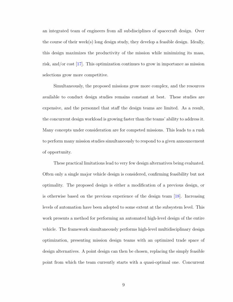
an integrated team of engineers from all subdisciplines of spacecraft design. Over
the course of their week(s) long design study, they develop a feasible design. Ideally,
this design maximizes the productivity of the mission while minimizing its mass,
risk, and/or cost [17]. This optimization continues to grow in importance as mission
selections grow more competitive.
Simultaneously, the proposed missions grow more complex, and the resources
available to conduct design studies remains constant at best. These studies are
expensive, and the personnel that staff the design teams are limited. As a result,
the concurrent design workload is growing faster than the teams’ ability to address it.
Many concepts under consideration are for competed missions. This leads to a rush
to perform many mission studies simultaneously to respond to a given announcement
of opportunity.
These practical limitations lead to very few design alternatives being evaluated.
Often only a single major vehicle design is considered, confirming feasibility but not
optimality. The proposed design is either a modification of a previous design, or
is otherwise based on the previous experience of the design team [18]. Increasing
levels of automation have been adopted to some extent at the subsystem level. This
work presents a method for performing an automated high-level design of the entire
vehicle. The framework simultaneously performs high-level multidisciplinary design
optimization, presenting mission design teams with an optimized trade space of
design alternatives. A point design can then be chosen, replacing the simply feasible
point from which the team currently starts with a quasi-optimal one. Concurrent
9

design teams would then conduct their full design study using the chosen design as
a starting point.
1.4.2 Prior Attempts to Automate Vehicle Design
The concept of employing automation to solve complex systems design prob-
lems is not novel. Several schemes have been developed which utilize GAs to perform
design optimization, dating back to at least the 1990s. Mosher created a basic GA
package for spacecraft design which could explore a large portion of a satellite de-
sign space, considering a large number of dissimilar spacecraft designs [19] (far more
than the less than ten designs usually considered by conventional mission design
teams). This allowed for a more complete exploration of the design space, unbiased
by previous experience of the design engineer.
Mosher used his framework to compare a complete enumeration approach and
a GA-based approach for a case study replicating the mission requirements for the
Near Earth Asteroid Rendezvous (NEAR) Shoemaker mission. Even with the enu-
meration approach, only one design was found that met all constraints. Interestingly,
the actual NEAR Shoemaker mission also failed to meet all specified constraints,
requiring a rocket modification. Several designs were found that were close to com-
pliance with the constraints. This indicates that there is an important value to
simply imposing a penalty function on designs that violate some constraints, rather
than immediately eliminating them.
10
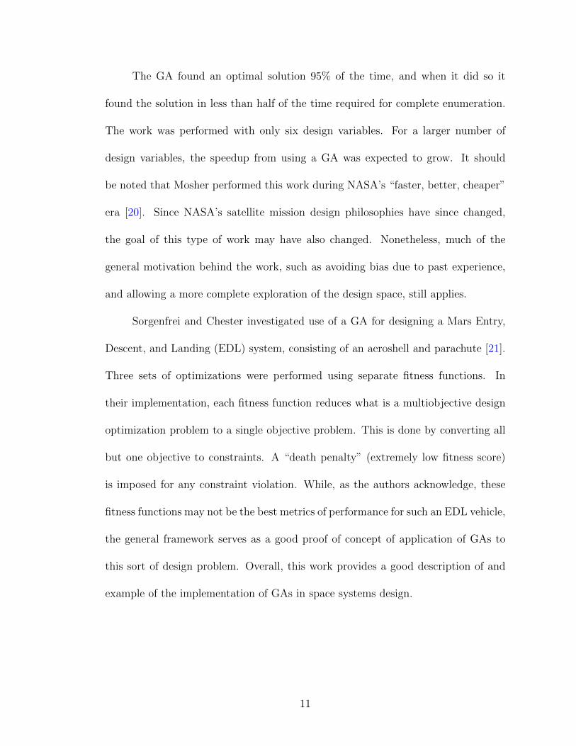
The GA found an optimal solution 95% of the time, and when it did so it
found the solution in less than half of the time required for complete enumeration.
The work was performed with only six design variables. For a larger number of
design variables, the speedup from using a GA was expected to grow. It should
be noted that Mosher performed this work during NASA’s “faster, better, cheaper”
era [20]. Since NASA’s satellite mission design philosophies have since changed,
the goal of this type of work may have also changed. Nonetheless, much of the
general motivation behind the work, such as avoiding bias due to past experience,
and allowing a more complete exploration of the design space, still applies.
Sorgenfrei and Chester investigated use of a GA for designing a Mars Entry,
Descent, and Landing (EDL) system, consisting of an aeroshell and parachute [21].
Three sets of optimizations were performed using separate fitness functions. In
their implementation, each fitness function reduces what is a multiobjective design
optimization problem to a single objective problem. This is done by converting all
but one objective to constraints. A “death penalty” (extremely low fitness score)
is imposed for any constraint violation. While, as the authors acknowledge, these
fitness functions may not be the best metrics of performance for such an EDL vehicle,
the general framework serves as a good proof of concept of application of GAs to
this sort of design problem. Overall, this work provides a good description of and
example of the implementation of GAs in space systems design.
11

1.4.3 Generalized Spacecraft Design
The above case studies in automated spacecraft design share a major draw-
back; they all utilize specialized schemes unique to their specific design problem.
Modification of any to address additional design problems would, optimistically,
require substantial modification of their existing problem framework. There have
been some prior investigations into possibilities for generalized spacecraft design. It
is largely this idea that is driving the adoption of MBSE.
One academic example of such an attempt is the work by Shaw to develop
a Generalized Information Network Analysis (GINA) methodology and model for
analyzing designs of any spacecraft or constellation of spacecraft [22]. The GINA
methodology treats any satellite system as an information transfer network. The
idea is that any space-based system (that is, a system involving a spacecraft or
collection of spacecraft) can be modeled as collecting information from some source,
processing that information, and transmitting it to some customer.
Shaw considered satellite navigation systems such as GPS, global communi-
cations networks such as Iridium, information transfer systems such as the many
proposed and operational satellite internet services, and global reconnaissance ser-
vices. While Shaw did not consider scientific space missions, it is clear that most
Earth science, planetary science, and astrophysics missions have analogues to the
mission types considered, with the caveat that substantial additional considerations
may be required for non-Earth-orbiting missions.
12
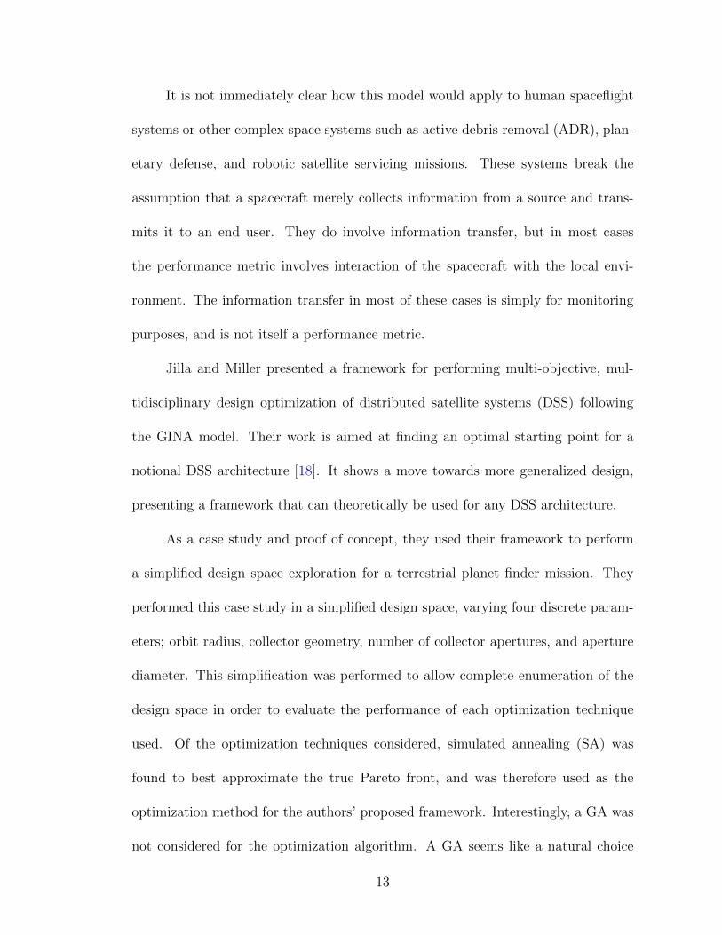
It is not immediately clear how this model would apply to human spaceflight
systems or other complex space systems such as active debris removal (ADR), plan-
etary defense, and robotic satellite servicing missions. These systems break the
assumption that a spacecraft merely collects information from a source and trans-
mits it to an end user. They do involve information transfer, but in most cases
the performance metric involves interaction of the spacecraft with the local envi-
ronment. The information transfer in most of these cases is simply for monitoring
purposes, and is not itself a performance metric.
Jilla and Miller presented a framework for performing multi-objective, mul-
tidisciplinary design optimization of distributed satellite systems (DSS) following
the GINA model. Their work is aimed at finding an optimal starting point for a
notional DSS architecture [18]. It shows a move towards more generalized design,
presenting a framework that can theoretically be used for any DSS architecture.
As a case study and proof of concept, they used their framework to perform
a simplified design space exploration for a terrestrial planet finder mission. They
performed this case study in a simplified design space, varying four discrete param-
eters; orbit radius, collector geometry, number of collector apertures, and aperture
diameter. This simplification was performed to allow complete enumeration of the
design space in order to evaluate the performance of each optimization technique
used. Of the optimization techniques considered, simulated annealing (SA) was
found to best approximate the true Pareto front, and was therefore used as the
optimization method for the authors’ proposed framework. Interestingly, a GA was
not considered for the optimization algorithm. A GA seems like a natural choice
13

for Pareto front identification. It naturally determines a Pareto front from an entire
“population” of designs, with well known multi-objective GAs such as NSGA-II well
documented in literature [23].
GINA is a powerful framework for evaluating design options, but does not
in-and-of itself perform design optimization. The goal of GINA is trade analysis
of systems that have already been designed. It provides a model through which
any architecture option can be interpreted, allowing a fair comparison to be made
between different architectures. GINA does not perform design of the spacecraft
itself. It models each satellite, subsystem, and ground station as a node of the
overall system. As will be detailed in this dissertation, the CR model and the
Generalized Evolutionary Spacecraft Design Architecture (GESDA), focus on the
space segment, and modeling the flow of multiple resources through the spacecraft
in a similar manner to which GINA models information flow.
1.5 Variable Length Genome GAs
Variable length genome GAs are useful for optimizing systems with a variable
number of design parameters. This naturally lends itself to CR problems, where the
optimal number of components may not be known a priori.
Previous investigations have considered the use of variable length genome GAs.
Lee and Antonsson proposed exG, a framework for managing a genome of varying
length [24]. In exG, a traditional single string genome is augmented with an index
string, each gene of which acts as an index for a corresponding data gene. Design
14

traits are assigned to ranges of the index string rather than to specific values of
the original encoding string. This allows genomes with a variable number of genes
describing each trait to be decoded assuming constant range bounds for the index
string.
Variable length crossover is achieved by picking a sub-range of the value bounds
for the index string, and exchanging genes within this range between the two parent
designs. The authors argue that this variable length genome (VLG) crossover oper-
ator eliminates the need for a VLG mutation operator that can change the genome
length. A dedicated mutation operator is not needed to change the length of a
genome. However, including a traditional mutation operator still seems necessary
to preserve the GA’s ability to add options not present in the population to the
encoding string, in order to avoid local minima.
Ting et al. [25] proposed use of a multiobjective variable-length genetic algo-
rithm to solve a heterogeneous transmitter placement problem. NSGA II is used for
genetic selection to handle the multiobjective nature of this design problem. The
algorithm used a variable length chromosome representation, due to the variable
number of components in potential design solutions. The authors proposed a novel
hybrid crossover, which uses varying combinations of uniform crossover between in-
dividual components and single point crossover of the entire parent chromosomes
by components. The latter allows the variable length chromosome GA to find the
optimal number of components, without the need for any length mutation operator.
More recently, Ryerkerk et al. investigated the performance of several variable-
size genetic algorithm implementations [15]. Their implementation involves a vari-
15

able length genome, and special recombination and mutation operators to handle
them. The variable-length cut-and-splice (based on the work of [25]), spatial re-
combination, and synapsing variable length crossover (SVLC) were evaluated. Ad-
ditionally, a new crossover operator, similar component crossover, was proposed.
This method attempts to perform respectful recombination by pairing similar com-
ponents, ensuring that a component of each pair will be inherited by each child
design.
All variable length operators with the exception of cut and splice performed
somewhat better than the fixed length representation, while cut and splice per-
formed far worse than the fixed length representation. When the optimal number
of components is not known a priori, use of a variable length crossover, proved de-
sirable. This is because it will optimize the number of components as well as the
configuration thereof.
The authors do note that in later generations, these schemes seem to become
stuck in sub-optimal solutions, which would require multiple concurrent mutations
to reach a better optimum. It may therefore be of interest to consider an algo-
rithm where the mutation rate increases in later generations, as improvement from
generation to generation slows.
1.6 The Present Work
Jilla and Miller’s work provides an interesting parallel to the work of this
dissertation. The motivation of their work is essentially identical. It served as a proof
16

of concept for the application of automated, metaheuristic design optimization in the
conceptional design phase. However, much like the body of work in the field, their
work was tailored to a specific problem. Nonetheless, the general DSS architecture
which they address is a broad design problem. Their work is therefore a substantial
step in the direction of generalized spacecraft design.
GINA is described by Shaw as being reduced to how to “move some entity from
one point to another in an underlying network...as effectively as possible, both to
provide good service to the users...and to use the underlying transmission facilities
effectively”. The goal of the CR model detailed in this dissertation can be similarly
described as analyzing the flow of multiple entities (resources) from sources to sinks.
These sources and sinks can be components within the system (spacecraft, in our
case), or exist outside of it (the Sun, for one example, being a radiation source in
our case).
1.6.1 The Problem Statement
The overarching purpose of this work is to develop a generalized framework
that can, with little to no modification, address any spacecraft design problem. The
framework must understand the objectives, constraints, and operating properties of
any spacecraft. For any payload and any relevant objectives, it must be able to
perform trade space exploration and multiobjective design optimization, producing
feasible, Pareto-optimal vehicle designs for the given mission.
17

1.6.2 Contributions of the Present Work
The first contribution of this work is somewhat standalone compared to the
others, though it does originally motivate them, and, ultimately, serve to validate
them. That contribution is an attempt at an objective comparison of proposed LEO
ADR payloads. The work of Chap. 2 in this dissertation presents the first attempt
at this. This work, along with parallel research being carried out by the author at
the time, motivated the generalized CR model that comprises the remainder of this
dissertation.
As has been alluded to, this work is not the first attempt to automate vehicle
design optimization, or even specifically spacecraft design optimization. Nor is it the
first attempt to create a generalized scheme for spacecraft trade space analysis. The
most significant contribution of this work is the CR model, which can be applied to
any spacecraft design. In fact, the CR model is generalizable to a much wider range
of systems engineering problems. Any system that can be modeled as a collection of
components and resources that flow between them can likely be addressed by this
model.
The goal of the CR model is to describe a complex system such as a spacecraft
in a way that the system and its operational constraints can be easily understood by
an algorithm, including metaheuristic optimization algorithms. The model provides
a uniform method of handling constraints of the whole system as well as of individual
components that comprise it.
18

This work presents a design optimization and trade space exploration frame-
work based around the CR model. This model allows generalized simulation and
optimization of a large class of complex systems including spacecraft design. It al-
lows such systems to be easily understood and processed by computer algorithms.
This facilitates automated optimization of complex multidisciplinary, multiobjective
problems. The CR model allows a computer to interpret complex systems, facili-
tating simulation, automated optimization, and trade space exploration. The latter
two are accomplished through a specialized variable length genome GA. The novel
genome encoding scheme and crossover operator developed for this GA comprise the
second contribution of the present work.
In the context of this work, the optimization problem is essentially a com-
ponent selection problem. Since the intended application of the work is spacecraft
design optimization, this component selection problem requires a library of space-
craft components. Aggregating proposed and historical spacecraft components is
a non-trivial task. Additionally, while the core CR model is applicable to a wide
range of problems, it must be combined with problem specific simulations and con-
siderations to create an optimization framework which allows the CR model to be
used for satellite design optimization. The third major contribution of this work is
therefore the spacecraft environment and component-level simulations required to
apply the CR model to spacecraft design optimization.
19

1.6.2.1 A Technology Comparison for Low Earth Orbit Active Debris
Removal
The first contribution of this work entails a GA-based vehicle designer which
takes the different ADR payloads as input, produces spacecraft around each of them,
and evaluates their performance conducting an active debris removal program. The
first attempt at this, for which the model was very problem-specific is presented in
Chap. 2. This problem is revisited with the generalized framework presented later
in this dissertation. This second analysis of the LEO ADR problem offers the ADR
vehicles in additional detail, with the problem setup and final results presented in
Chap. 9.
1.6.2.2 The Component-Resource Model
The most significant contribution of this work is the component-resource (CR)
model it proposes. Many complex systems, including all spacecraft, can be modeled
as a collection of components and resources that flow between them. Each compo-
nent can be a source, sink, or store (referred to in general as nodes) for each resource
within the system. Sources produce a resource, sinks consume a resource, and stores
contain an internal reservoir for a resource, operating as a source or sink depending
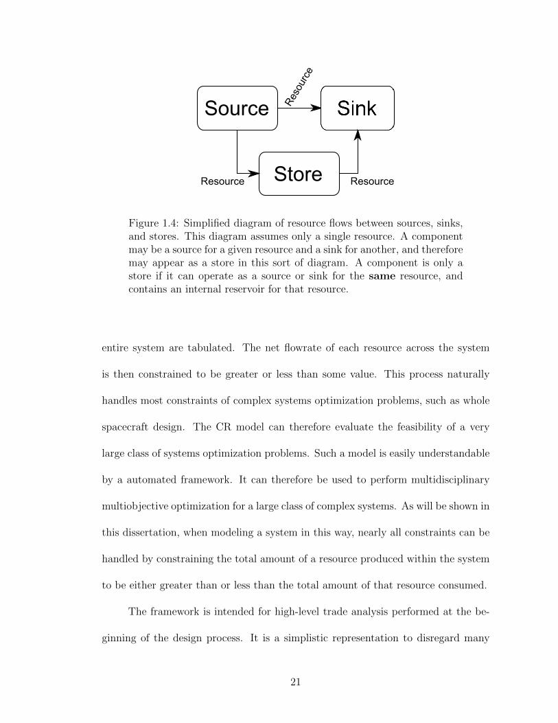
on the state of the rest of the system, as indicated by Fig. 1.4. A given component
may be a source, sink, and/or store simultaneously for different resources or differ-
ent states of the system. Flowrates of resources produced and consumed across the
20
Source
Resource
StoreResource Resource
Figure 1.4: Simplified diagram of resource flows between sources, sinks,and stores. This diagram assumes only a single resource. A componentmay be a source for a given resource and a sink for another, and thereforemay appear as a store in this sort of diagram. A component is only astore if it can operate as a source or sink for the same resource, andcontains an internal reservoir for that resource.
entire system are tabulated. The net flowrate of each resource across the system
is then constrained to be greater or less than some value. This process naturally
handles most constraints of complex systems optimization problems, such as whole
spacecraft design. The CR model can therefore evaluate the feasibility of a very
large class of systems optimization problems. Such a model is easily understandable
by a automated framework. It can therefore be used to perform multidisciplinary
multiobjective optimization for a large class of complex systems. As will be shown in
this dissertation, when modeling a system in this way, nearly all constraints can be
handled by constraining the total amount of a resource produced within the system
to be either greater than or less than the total amount of that resource consumed.
The framework is intended for high-level trade analysis performed at the be-
ginning of the design process. It is a simplistic representation to disregard many
21

holistic system aspects and decisions, such as, in the case of satellite design, the me-
chanical configuration of the spacecraft. However, even with these simplifications,
quality trade analysis is possible as long as these simplifications are made uniformly
among all design options considered.
As has been stated, the underlying principles of the framework are easily
transferable to a large class of systems engineering problems. Any system that
can be defined as a collection of components and resources that flow between them
can be analyzed using the CR model. Therefore, an attempt will be made when
describing the framework to speak generally about systems, rather than specifically
about spacecraft.
1.6.2.3 The Vehicle Encoding Genetic Algorithm
The third major contribution is the specialized genetic algorithm developed
for optimization. The CR model frames problems of interest as component selection
problems. The Vehicle Encoding Genetic Algorithm (VEGA) provides an encoding
mechanism for defining system designs as an organized collection of components, as
well as a GA for optimizing designs using this encoding scheme. Each gene in an in-
dividual genome corresponds to a single component in the system. A variable length
GA is therefore utilized to optimize the number of components as well as the specific
combination of components. This includes a variable length crossover operator and
a division of the genome into individual “chromosomes” for each component class.
22

1.6.2.4 A Generalized Evolutionary Spacecraft Design Architecture
The final contribution is the specific spacecraft design architecture, built around
the CR model. This entails the definition and initial population of a spacecraft
component library and the associated simulations, both at a system or environment
level, and at an individual spacecraft component level. In practice, the component
libraries are largely drawn from NASA’s Satellite Parts On-Orbit Now (SPOON)
database [26]. It is therefore acknowledged that the component libraries presented
here do not themselves constitute a contribution.
The remainder of this contribution is the associated spacecraft and component-
level simulations. Great effort was made throughout the development of this space-
craft design analysis framework to preserve generality across different space missions,
allowing the framework to be applied to a wide range of missions with little to no
modification.
1.7 Content of the Document
The remainder of this dissertation is outlined as follows. Chap. 2 presents
a conventional spacecraft design optimization problem; the design of active debris
removal spacecraft to operate in LEO. This problem motivates the development of
the CR model in the remaining chapters of this dissertation.
Chap. 3 presents the simplest form of the CR model; the general static CR
model. In the static model, all resource flows are steady state. Tabulating resource
relations once for a given system snapshot is sufficient to fully understand the be-
23

havior and feasibility of the system. The basic functioning of components as sources,
sinks, and stores is discussed in detail. Resource flow in this case is also described,
and an example is detailed to make clear how this most basic form of the model
functions.
Chap. 4 describes the optimization model and GA developed for this disser-
tation. It details the different levels of the genome, describing the collection of
components present, properties of an individual component, and system-level prop-
erties. It also describes the form of the GA itself. A particular focus is given to
the selection and crossover operators developed, and genome structure. The chapter
demonstrates how the framework handles single objective and multiobjective prob-
lems. It discusses the internal constraint handling process, particularly how resource
relations implicitly handle most component and system level constraints.
Chap. 5 provides a simple example of a Static CR design problem, working
through setting up the design problem in the context of the CR model. It compares
optimization results obtained with the theoretical optimum for that design problem.
Chap. 6 extends the CR model to dynamic problems, where the system be-
havior changes over time. This is important for the spacecraft design problem, since
spacecraft behavior changes over the course of an orbit or interplanetary trajectory,
as well as between the multiple operating modes a spacecraft may have. Dynamic
resource availability over time within a given mode will be discussed, in particular
focusing on edge resources, which flow between the system and the environment.
Chap. 7 uses the framework developed in Chaps. 3-6, presenting the satellite
framework based on the CR model and VEGA. It covers the specific resources
24
included for this set of design problems, the spacecraft component classes developed,
and simulation and fitness score evaluation for space missions.
Chap. 8 presents a mission concept for a Earth imaging satellite used to develop
and verify the framework. The LEO ADR design problem of Chap. 2 is revisited
with the framework in Chap. 9, serving as an ultimate benchmark of the framework.
Finally, Chap. 10 presents some conclusions and areas identified for further
future investigation.
25

Chapter 2: LEO Active Debris Removal Technology Assessment
2.1 Overview
On-orbit satellite debris is a growing problem, particularly in LEO [9]. The
continuous growth in the number of objects on orbit increases the likelihood of an
ablation cascade, a catastrophic series of collisions initiated by the destruction of a
small number of large objects on orbit [11]. Such an event would result in debris
clouds that could render many common orbits unusable. Several technologies have
been proposed to address the growing debris problem using airborne, ground-based,
and space-based systems. The work detailed in this chapter evaluates and compares
proposed orbital technologies for removing debris objects (DOs) from LEO. The fo-
cus was placed on large intact debris objects, since a collision with one of these could
produce many small fragments, each of which could lead to additional collisions.
To perform this comparison, spacecraft were designed around several proposed
active debris removal payloads. A genetic algorithm was employed to find the most
efficient designs for orbital debris removal, with special attention given to minimizing
the financial cost of such systems, and the risk they pose to infrastructure and human
life in orbit and on the ground. Listings of the Pareto-optimal designs are presented
at the end of the chapter.
26
The work detailed in this chapter is intended to provide an objective compar-
ison of proposed orbital solutions that remove large, intact objects from low Earth
orbit. To accomplish this, a satellite design software package was developed to pro-
duce spacecraft that utilize the proposed active debris removal (ADR) technologies.
Designs were selected for further investigation based on financial cost per object
removed and risk to infrastructure and human life, both in orbit and on the ground.
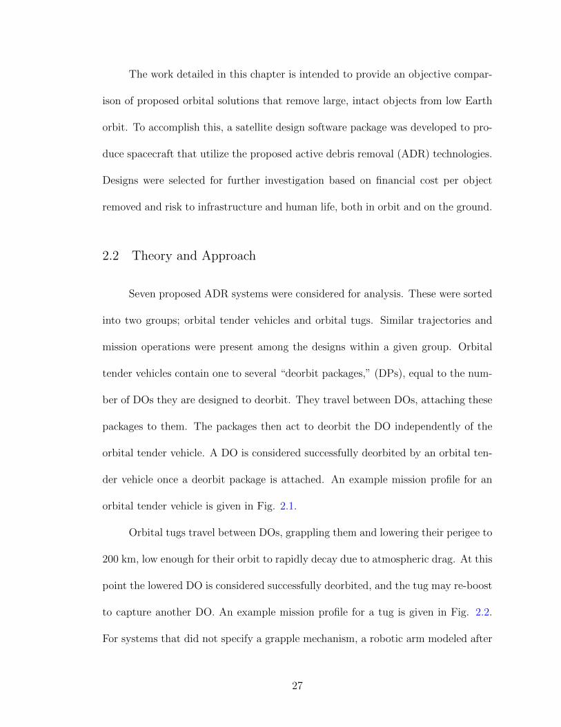
2.2 Theory and Approach
Seven proposed ADR systems were considered for analysis. These were sorted
into two groups; orbital tender vehicles and orbital tugs. Similar trajectories and
mission operations were present among the designs within a given group. Orbital
tender vehicles contain one to several “deorbit packages,” (DPs), equal to the num-
ber of DOs they are designed to deorbit. They travel between DOs, attaching these
packages to them. The packages then act to deorbit the DO independently of the
orbital tender vehicle. A DO is considered successfully deorbited by an orbital ten-
der vehicle once a deorbit package is attached. An example mission profile for an
orbital tender vehicle is given in Fig. 2.1.
Orbital tugs travel between DOs, grappling them and lowering their perigee to
200 km, low enough for their orbit to rapidly decay due to atmospheric drag. At this
point the lowered DO is considered successfully deorbited, and the tug may re-boost
to capture another DO. An example mission profile for a tug is given in Fig. 2.2.
For systems that did not specify a grapple mechanism, a robotic arm modeled after
27

Figure 2.1: Orbital tender vehicle mission profile, shown here with agossamer sail deorbit package as an example.
the Orbital Express Demonstration Manipulator System (OEDMS) [27] was used.
This arm was assumed to have a mass of 71 kg, require 131 W while operating, and
to be currently developed to Technology Readiness Level (TRL) 7, for the purpose
of this debris removal mission. The next two sections provide details of the proposed
ADR systems, suggested by previous work, that were considered in this analysis.
2.2.1 Deorbit Packages Included in Analysis
All DPs considered here were assumed to require no power draw from the
tender vehicle except in some cases during initial deployment, once the DP has
been attached to the DO. With the exception of Terminator Tether, all DPs listed
here worked by increasing the surface area, and therefore decreasing the ballistic
coefficient of the DO, increasing drag to shorten its lifetime on orbit. For the
purposes of this analysis, it was assumed that once a DP is attached to a DO and
28

Figure 2.2: Tug mission profile, shown here with a laser ablation tug(LAT) as an example.
released by the tender vehicle, the mass of that DP can be completely subtracted
from the total mass of the tender vehicle. Furthermore, it was assumed that the
attachment of DPs to the DOs requires no additional hardware beyond that stated
below, with the exception of a robotic arm for initial attachment. It is assumed
that the manipulator described above can perform this task itself without additional
hardware.
Table 2.1: Deorbit Package Parameters.
ADR system Mass (kg) Power (W)
KSII 74 10TRIS 106 1
GOLD 70 0Terminator Tether 28 0
29

2.2.1.1 KnightSat II (KSII)
KSII was a self-contained Gossamer Sail (aerodynamic decelerator) proposed
by the University of Central Florida [28]. It utilizes magnetic torque rods for attitude
control. The mass and power consumption assumed for KSII are given in Table 2.1.
2.2.1.2 L’Garde Towed Rigidizable Inflatable Structure (TRIS)
The TRIS is a self-contained aerodynamic decelerator based on a device tested
on STS-77 [29]. TRIS includes a dish-like decelerator deployed and supported by
inflatable, rigidizable booms. The mass and power consumption assumed for the
TRIS are given in Table 2.1.
2.2.1.3 Gossamer Orbit Lowering Device (GOLD)
GOLD is a self-contained DP developed by Global Aerospace Corporation and
ILC Dover [30]. It comprises an inflatable Gossamer sphere that can be attached
to a DO and then remotely or autonomously inflated at a later point. The device
has the ability to modulate the extent to which it is inflated at lower altitudes to
facilitate targeted reentry. The GOLD package contains its own solar power system,
so it does not impose a power requirement on the DO or tender vehicle. The mass
assumed for GOLD is given in Table 2.1.
30

2.2.1.4 Terminator Tether
Terminator Tether was a self-contained DP developed by Tethers Unlimited
[31]. Terminator Tether comprises a several kilometer long electrodynamic drag
tether that deorbits the DO and provides electrical power to the system. Terminator
tether is stated as having a mass of 1-2% of the DO, so a worst case 28 kg was
assumed for the DO population described above.
2.2.2 Orbital Tug ADR Systems Included in Analysis
The following ADR technologies, suggested by previous work, were considered
for this analysis. The mass and power requirements for each tug ADR system are
provided in Table 2.2.
Table 2.2: Orbital Tug Payload Parameters.
ADR system Mass (kg) Power (W)
EDDE 80 0LAT 42 250
Conventional Tug 0 0
2.2.2.1 Electro-Dynamic Debris Eliminator (EDDE)
EDDE [32] is a several kilometer long conducting tether, with solar panels
spaced periodically along its length, and with avionics and capture nets at either
end. It uses electric current through and around the tether to produce a force
perpendicular to the Earth’s magnetic field, enabling it to maneuver throughout
31

low Earth orbit. Upon arriving at a DO, EDDE rotates perpendicular to the tether
axis with a net deployed at one end to capture the DO. The DO is then maneuvered
to a 330 km disposal orbit, where it is released.
For the purpose of this analysis, based on published proposals for EDDE, the
system was assumed to be self-contained. That is, no external support hardware was
required, and the quoted size and mass included all required subsystems, including
ADR, propulsion, and DO capture mechanism. It is of note that EDDE is the only
self-contained technology considered in this analysis. The fundamentally unique
nature of EDDE makes it unrealistic to simply model it as a payload on an otherwise
conventional spacecraft, as was done with the other technologies.
2.2.2.2 Laser Ablation Tug (LAT)
The LAT [33] features a pulsed laser that repeatedly ablates small portions
of surface material from the DO, producing net thrust in a desired direction. Since
this ADR technology ablates the surface of an attached DO, there is no need to
carry a dedicated onboard propellant supply. Upon detaching from a DO, the LAT
separates a small portion of the DO, which it keeps to use as propellant to reach its
next target.
2.2.2.3 Conventional Tug
A conventional tug was also included in this analysis as a baseline ADR vehicle,
against which to compare the other proposed ADR technologies. The conventional
32

tug is simply a spacecraft with a manipulator to grapple a DO, and a flight proven
propulsion system to maneuver the DO into a disposal orbit. No additional ADR
system is present, so the ADR system for a conventional tug is modeled as having
no mass and requiring no power.
2.2.3 ADR Vehicle Design Optimizer
Vehicle design optimization software was developed to generate vehicles, each
based upon a proposed ADR technology. A genetic algorithm was used to optimize
vehicle designs, minimizing the financial cost per DO removed and the risk posed
by debris removal. The properties listed in Table 2.3 were assumed for each ADR
system. In the case of EDDE, actual thrust values were not available, so rated
altitude and plane change rates were used instead, as listed in Table 2.3.
Table 2.3: ADR System Parameters.
ADRsystem
CircularizingThrust
∆ΩThrust
DeorbitThrust
Self-Propelling?
Self-Contained?
Self-Grappling?
KSII - - - No No NoTRIS - - - No No No
GOLD - - - No No NoT. Tether - - - No No No
EDDE 4.4 m/s 1.4/day 4.4 m/s Yes Yes YesLAT 0.035 N 0.035 N 0.035 N Yes No No
Conv. Tug - - - No No No
33

Figure 2.3: Top-level ADR design optimizer algorithm.
2.2.3.1 Vehicle Designer
Vehicle designs were generated as described below, with the top-level design
optimization process as depicted in Fig. 2.3. The design of each vehicle was based
on an input parameter array that serves as the genome for the genetic algorithm,
described below. Each genome is composed of several input parameters (IP i, where
i is the input parameter in question). An example genome is shown in Fig. 2.4, and
a brief description of each input parameter is given in Table 2.4. A listing of the
potential values for each input parameter is given in Appendix A. IP1 designates
the ADR system a vehicle carries, and IP2 designates the thruster to be used as
the dedicated propulsion system (DPS). A key of potential options for IP1 and IP2
is given in Table 2.5. In some cases, multiple thrusters of a single type (e.g. ion
34
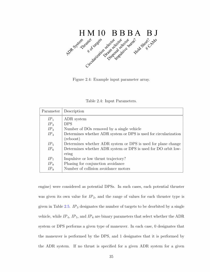
Figure 2.4: Example input parameter array.
Table 2.4: Input Parameters.
Parameter Description
IP1 ADR systemIP2 DPSIP3 Number of DOs removed by a single vehicleIP4 Determines whether ADR system or DPS is used for circularization
(reboost)IP5 Determines whether ADR system or DPS is used for plane changeIP6 Determines whether ADR system or DPS is used for DO orbit low-
eringIP7 Impulsive or low thrust trajectory?IP8 Phasing for conjunction avoidanceIP9 Number of collision avoidance motors
engine) were considered as potential DPSs. In such cases, each potential thruster
was given its own value for IP2, and the range of values for each thruster type is
given in Table 2.5. IP3 designates the number of targets to be deorbited by a single
vehicle, while IP4, IP5, and IP6 are binary parameters that select whether the ADR
system or DPS performs a given type of maneuver. In each case, 0 designates that
the maneuver is performed by the DPS, and 1 designates that it is performed by
the ADR system. If no thrust is specified for a given ADR system for a given
35

Table 2.5: Input parameter key for IP1 and IP2.
IP1 Value ADR system IP2 Value Thruster Type
B KSII B-H BipropellantC Conventional
TugI-O Monopropellant
D TRIS P ResistojetE EDDE Q-R ArcjetF GOLD S Pulsed Plasma
ThrusterG Terminator
TetherT-Z Hall Effect
ThrusterH LAT a-e Ion Engine
f-i No DPS
maneuver type, the input parameter for that maneuver type will be forced to 0.
IP4 selects for circularization or orbit raising (depending on whether impulsive or
low thrust) maneuvers, which return the vehicle to the orbit occupied by the DOs.
IP5 selects for plane change maneuvers. In the case of low thrust maneuvers, plane
change is performed as part of the orbit raising and disposal maneuvers, so the
parameter is ignored. IP6 selects for disposal maneuvers, which lower the DOs
perigee altitude to 200 km. A DO being removed by an orbital tender vehicle was
considered removed upon attachment of the DP to the DO, so this parameter was
ignored for orbital tender vehicles. IP7 dictates whether maneuvers performed by
the vehicle are impulsive or low thrust, IP8 designates whether a vehicle should
perform phasing conjunction avoidance while crossing high priority orbits (see risk
factors section below), and IP9 designates how many collision avoidance motors
should be added to the vehicle.
36

An overall risk factor ORF was assigned to each vehicle produced. This was
used to quantify the risk posed by each design to people and property in orbit
and on the ground. r was determined through the combination of several factors
influencing the risk of a given design. An in-depth discussion is provided in the risk
factors section below.
Based on a given genome, individual vehicles were designed following the pro-
cess shown in Fig. 2.5. A maneuver table was produced, detailing the ∆V required,
the propulsion system used, and the mass of any object attached to (or removed
from) the vehicle for each maneuver, from the last maneuver the vehicle produced to
the first. The maneuver table produced was based on the mission profiles described
in Fig. 2.1 and Fig. 2.2. For the purposes of this simulation, vehicle life was limited
to fifteen years. A manipulator was added to vehicles for which the ADR system
did not have self-grappling capability for grappling DOs. The payload mass for the
vehicle was assumed to be the combined mass of the ADR system and manipulator,
if present.
With the exception of self-contained ADR systems, the mass of the spacecraft
excluding the mass of the DPS and electrical power system (EPS) was assumed
to be 2.33 times the payload mass, based on historical data [34]. The total power
requirement was defined as the greatest maximum power requirement among the
ADR system, manipulator, or DPS. Note that this implies that the ADR system,
manipulator, and DPS never operate at the same time. An additional load was
added to this value for command and data handling and communications. This
requirement was multiplied by a factor of 1.31 to account for losses within the
37

Figure 2.5: Individual vehicle design process.
EPS [17]. Based on this power requirement and the given DO orbit, an EPS was
produced for the vehicle that included triple junction GaAs photovoltaic arrays for
power generation.
A propulsion system was then produced based on the vehicle mass thus far and
the vehicles maneuver table, following the process shown in Fig. 2.6. This included
the mass of the DPS, propellant, and propellant tank. Collision avoidance motors
were attached as dictated by the genome. The motors were designed to provide a
∆V of 0.3 m/s each, enough to lower the perigee of the orbit by 1 km. The vehicle
designer was iterated until the total vehicle mass converged, or the mass exceeded
existing or near future launch capability, assumed to be 70 metric tons to low Earth
orbit [35]. Once the mass converged, a mission timeline was calculated based on
38

Figure 2.6: Propulsion system design process.
the maneuver times, with three days added per DO, dedicated to rendezvous and
grappling. The required fleet size was then determined, ensuring enough vehicles to
remove 100 DOs, at a rate of at least 10 DOs per year.
Development and production costs were determined in 2014 USD using the
Spacecraft/Vehicle Level Cost Model [36]. Launch costs were determined based on
published prices of actual launches on commercially available launch vehicles. Based
on these, a linear fit of CLV = 0.0094mtot + 18 was developed to determine launch
cost, where CLV is the launch cost in millions of 2014 USD, and mtot is the vehicle
total mass in kg. For payloads that were known to be small enough and light enough
to fit into a single slot on an EELV Secondary Payload Adapter (ESPA) ring [37],
it was determined whether doing so would decrease the launch cost, assuming $3M
39

per ESPA slot. The ADR vehicle was assumed to be launched on an ESPA ring
when doing so was less expensive than the launch cost given by the function for
CLV above, and vehicles launched on an ESPA ring were assumed to be delivered
directly to the orbit of the first DO to be removed.
2.2.3.2 Risk Factors
Each vehicle design was assessed to determine the overall risk it would pose to
active hardware and human life, in orbit and on the ground. This risk factor roughly
represents the expected value lost inadvertently as a result of a given ADR program,
with units of active scientific spacecraft. For example, a system with ORF = 0.5
roughly corresponds to a loss of value equal to half the cost of a single scientific
satellite mission over the course of the ADR program. While this comparison was
used to develop much of the logic of the risk evaluation, it should only be considered
valid for determining trends for comparing proposed ADR vehicles. It should not be
assumed without future work that these numbers accurately denote the actual loss
of value from execution of these programs. The remainder of this subsection details
the basis for the formulation of ORF , the overall risk factor. ORF is the sum of
two partial risk factors; the trajectory risk RT and the technology development risk
RTRL.
RT quantifies risk due to the trajectory of the ADR vehicles and DOs take in
Earth orbit and during reentry. Specifically, it addresses how these trajectories cross
the orbits of operational satellites as well as the uncertainty in potential ground
40

impact locations of the DOs. RT represents value lost directly through damage
caused by the debris removal program. A system was considered high risk if it could
not perform a reentry targeting a safe drop zone on the surface of the Earth. It was
considered medium risk if it was not high risk but could cross the orbit of a high
priority spacecraft, such as a manned spacecraft, and low risk if it was neither high
nor medium risk. An entry was considered targeted if it could be conducted within
three orbits from a low (disposal) orbit, after holding in a higher orbit for a period
of at least a week. It was assumed that variations in the atmosphere below 200 km
make orbital decay unpredictable once an object reaches this region.
An entry simulation including an atmospheric model was implemented to de-
termine whether or not a given ADR system was high risk or medium risk. An
example entry profile is shown in Fig. 2.7. In the figure, each of the horizontal bars
indicates a simulated high priority orbit. The beginning of targeted reentry opera-
tions is indicated where the rate of altitude loss decreases substantially, around 334
days in Fig. 2.7, indicating that the vehicle has halted orbit lowering operations.
After the Earth has rotated such that the DO orbit passes over an acceptable drop
zone, the ADR system is re-activated for a rapid reentry. Entry plots for each ADR
system are given in Fig. 2.8, with the exception of Terminator Tether. This excep-
tion is due to Terminator Tether’s ability to retract for phasing, collision avoidance,
and targeted reentry. Such an ability removes the need and benefit from performing
such an atmospheric simulation at this design phase. In the simulations performed
for this work, the orbits of the NASA A-Train, the Hubble Space Telescope, and
the International Space Station (ISS) were included as high-priority orbits, repre-
41
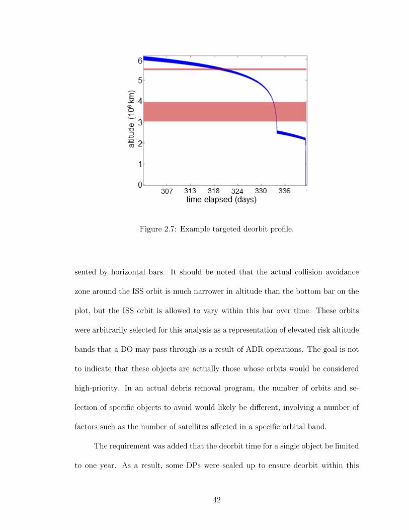
Figure 2.7: Example targeted deorbit profile.
sented by horizontal bars. It should be noted that the actual collision avoidance
zone around the ISS orbit is much narrower in altitude than the bottom bar on the
plot, but the ISS orbit is allowed to vary within this bar over time. These orbits
were arbitrarily selected for this analysis as a representation of elevated risk altitude
bands that a DO may pass through as a result of ADR operations. The goal is not
to indicate that these objects are actually those whose orbits would be considered
high-priority. In an actual debris removal program, the number of orbits and se-
lection of specific objects to avoid would likely be different, involving a number of
factors such as the number of satellites affected in a specific orbital band.
The requirement was added that the deorbit time for a single object be limited
to one year. As a result, some DPs were scaled up to ensure deorbit within this
42

Figure 2.8: Entry profiles based on ADR system and atmospheric simulation.
43
time frame. The values provided in Table 2.1 take this scaling into account. As
an example, KSII was scaled up from 9 m2 to 1000 m2 in order to meet the one
year deorbit requirement, increasing the systems mass from 15 kg to 74 kg. This
is a highly optimistic scaling, ignoring many of the complexities associated with a
device of the required size for the intended debris removal. However, as will be
shown below, even these scaled versions of DPs do not appear on the Pareto front,
so the oversimplifications made do not have a meaningful impact.
KSII can perform active attitude control using magnetic torque rods. It was
therefore assumed that its gossamer sail can be turned edge on to the direction of
travel, reducing the aerodynamic cross section to that of the DO. This ability could
be used to dramatically slow the DOs descent, allowing it to be parked in a low
orbit (200-300 km). The sail can later be returned to its original attitude, allowing
for targeted reentry. For KSII, crossing the A-train will require one to two months,
creating a risk of a conjunction between a DO being deorbited and a high-value
observatory. Therefore, KSII is assessed as medium risk. GOLD has the ability to
partially deflate its spherical envelope at lower altitudes. This causes the envelope to
assume an ellipsoidal shape, decreasing its aerodynamic cross section, and slowing
orbital decay. The envelope can then be re-inflated to the original cross section,
which allows for targeted reentry. GOLD is therefore assessed as medium risk.
TRIS is assumed to have no actuation capability after deployment. It is therefore
unable to perform targeted reentry, and assessed as high risk.
For conventional tugs, the ADR specific risk is a function of the propulsive
capability of the DPS. This splits these vehicles into two categories: those that
44

perform impulsive maneuvers for deorbit, and those that perform non-impulsive low
thrust maneuvers for deorbit. In the former case, it is assumed that the vehicle
performs a 175 m/s braking maneuver while grappling the DO, releases the DO,
and immediately performs a 175 m/s recircularization maneuver. This V places
the debris on a trajectory where it will be deorbited within three orbits, allowing
for targeted reentry and avoidance of high value orbital objects. Therefore, the
impulsive conventional tug is assessed as low risk. The low thrust conventional tug
applies a continuous retrograde thrust to the DO until it reaches a 200 km orbit,
at which point it disengages and raises its own orbit, and the DO is deorbited by
aerodynamic drag within a month. Since the time of terminal entry cannot be
predicted within a resolution of a few orbits, targeted reentry is not possible, and
therefore a low thrust conventional tug is assessed as high risk.
The LAT is stated as capable of performing a ∆V of 306 m/s, over 30 days
while attached to a 300 kg DO [33], reducing its orbital altitude below the ISS.
It was assumed that this was accomplished through constant low thrust, resulting
in a thrust of 0.035 N. The LAT can also halt orbit lowering to avoid high value
spacecraft while passing through their orbit.
Given EDDEs maneuvering capability of 380 km per day in the orbit of the
DOs while not carrying a DO [32], it is expected that EDDE can lower the orbit of
a 1400 kg DO by approximately 20.5 km per day. However, neither EDDE nor the
LAT can perform a targeted reentry without themselves entering the atmosphere.
Therefore, both are assessed as high risk.
45

Trajectory risk was defined as
RT = (N − nCAMNF )aRM +NRH (2.1)
where N is the total number of DOs that an ADR program is to deorbit, and nCAM
is the number of collision avoidance motors attached to each vehicle, detailed below.
NF is the number of ADR vehicles involved in the debris removal program. For any
medium or high risk ADR system, RM , representing the risk of collision with an
active spacecraft, was set to 10−3. This is derived from the fact that 1 in 1000 is
considered the threshold of acceptable risk of collision for a conjunction involving
an active satellite. That is, any higher risk of collision would warrant performing a
collision avoidance maneuver [38]. It was therefore concluded that a loss of value of
one thousandth the cost of a NASA robotic spacecraft is considered acceptable, per
conjunction. It is required that the risk of human casualty from any deorbit activities
be no greater than 1 in 10,000 [39]. Due to the size and structure of the DOs to
be deorbited, any high trajectory risk system, which does not possess the ability to
perform controlled entry of DOs, is assigned a value of 10−2 for RH , the lost value
associated with harm to people and objects on the ground. This is based on the
fact that acceptable risk of collision with a robotic spacecraft is ten times as great
as acceptable risk for collision with ground objects. For medium and low trajectory
risk systems, RH was set to 0, indicating that targeted DO reentry assumes no risk
to people or property on the ground. For low trajectory risk systems, RM was also
46
set to 0, indicating that the ADR system includes the capability to avoid collisions
with high priority objects on orbit.
A parameter (a) was included to account for the risk that debris removal poses
to any active satellite or other large DO crossing or nearing the orbit of the object
being removed. A destructive collision was assumed if this object came within a
keep-out zone extending 200 m in every direction from the structure of the ADR
system, ADR vehicle, or DO being deorbited, based on the keep-out sphere enforced
for the ISS [40]. (a) was defined as
a =AADRADO
(2.2)
where AADR is the destructive collision cross section of the mated stack, and ADO is
the destructive collision cross section of the DO alone. For tugs, AADR includes the
body of the tug and the geometry of the DO. For tender vehicles, AADR includes
the geometry of the deployed DP and DO. Destructive collision cross sections are
listed for each ADR system and for an unmitigated DO in Table 2.6, along with the
corresponding values for (a). It should be noted that GOLD and Terminator Tether
do in fact produce an increased cross section when deployed. However, GOLD claims
that an impact would not be destructive for the impacting object, and Terminator
Tether can be rapidly retracted to avoid a collision. Therefore, these systems are
assessed as having the same destructive collision cross section as the unmitigated
DO.
47

Table 2.6: Destructive collision cross sections.
ADR system Cross Section a
Unmitigated DO 129,000 m2 1Conventional Tug 129,000 m2 1
KSII 151,000 m2 1.17TRIS 156,000 m2 1.21EDDE 1.76 x 10⁶ m2 13.6GOLD 129,000 m2 1
Terminator Tether 129,000 m2 1LAT 129,000 m2 1
In order to avoid an impending (within a few orbits) conjunction with another
orbiting object, the vehicle designer contains the option for an ADR vehicle to carry
one or more collision avoidance motors. These are sized by the vehicle designer to
provide enough impulse to lower the perigee of the vehicle by 1 km. Adding these
motors mitigates the effect of RM by eliminating the risk of collision with some
number of active spacecraft. Each motor is assumed to eliminate the risk that a
single DO will collide with an active satellite. Therefore, the maximum number of
collision avoidance motors for a spacecraft was set as the number of DOs that a
single vehicle in the program is designed to remove.
The total trajectory risk for a given ADR system was determined as the sum
of the total risk to objects on the ground and the total risk to satellites of interest
in orbit. Total risk to objects on the ground is determined by multiplying RH by
N . Total risk to orbits of interest is similarly determined by multiplying RM by
the number of DOs deorbited without some collision avoidance mechanism. In the
current iteration, the only collision avoidance mechanisms are the collision avoidance
48
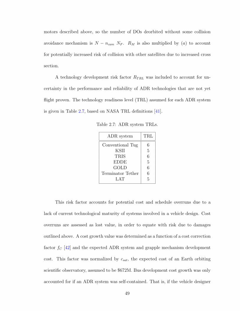
motors described above, so the number of DOs deorbited without some collision
avoidance mechanism is N − ncam NF . RM is also multiplied by (a) to account
for potentially increased risk of collision with other satellites due to increased cross
section.
A technology development risk factor RTRL was included to account for un-
certainty in the performance and reliability of ADR technologies that are not yet
flight proven. The technology readiness level (TRL) assumed for each ADR system
is given in Table 2.7, based on NASA TRL definitions [41].
Table 2.7: ADR system TRLs.
ADR system TRL
Conventional Tug 6KSII 5TRIS 6EDDE 5GOLD 6
Terminator Tether 6LAT 5
This risk factor accounts for potential cost and schedule overruns due to a
lack of current technological maturity of systems involved in a vehicle design. Cost
overruns are assessed as lost value, in order to equate with risk due to damages
outlined above. A cost growth value was determined as a function of a cost correction
factor fC [42] and the expected ADR system and grapple mechanism development
cost. This factor was normalized by csat, the expected cost of an Earth orbiting
scientific observatory, assumed to be $672M. Bus development cost growth was only
accounted for if an ADR system was self-contained. That is, if the vehicle designer
49

was designing a bus for the ADR system, was assumed that the bus was developed
with flight-proven technologies. For self-contained ADR systems, the TRL of the
bus was determined based on the spacecraft design details given by the author for
that ADR system. A risk factor was also added to account for the expected schedule
slippage based on TRL. A relative schedule slippage
RSS = 8.29e−0.56(WTRL) (2.3)
was assessed based on the work of Dubos, Saleh, and Braun [43], where WTRL is
the weighted sum of the TRL and development cost of each subsystem, divided by
the total development cost. To determine WTRL, the entirety of the spacecraft,
with the exception of the grapple mechanism and ADR system, was considered
to be a single subsystem with a TRL of 9 for non-self-contained systems. For
self-contained systems, a TRL was determined based on provided details, with the
relative schedule slippage being based on the lowest TRL subsystem. To determine
the total schedule slippage, this relative schedule slippage was multiplied by an
assumed development time of five years. The main risk associated with schedule
slippage is that additional catastrophic collisions will occur in low Earth orbit due
to the unmitigated debris during the schedule delay. This risk is assumed to result
in an additional seven collisions over the next two hundred years per forty years
of schedule slippage [9]. A nominal five year development schedule is assumed
for a given vehicle. Therefore, the absolute schedule slippage for this program
is determined by multiplying the relative schedule slippage by five. Multiplying
50
the above collision rate by the absolute schedule slippage results in a number of
additional collisions equal to 7/8 times the relative schedule slippage. Therefore,
the total risk factor from technology readiness is
RTRL =[Σ(fc − 1)cdev]
csat+
7
8RSS =
covcsat
+7
8RSS (2.4)
The final overall risk factor is then
ORF = RT +RTRL (2.5)
2.2.4 Genetic Algorithm
An initial generation of vehicles was produced based on random genomes. A
genetic algorithm was implemented to produce successive generations of designs.
The process followed by the genetic algorithm is shown in Fig. 2.9. To produce a
new generation, a fitness score is assigned to each member of the current generation.
The fitness function, determined heuristically, is given in Eq. 2.6:
fr = [10cDO(tPO)(ORF 3)]−1 (2.6)
Vehicle fitness is based primarily on the cost per DO removed, CDO, and the overall
risk of the ADR program, ORF . There is also some dependence on the time per
DO removed per ADR vehicle, tPO, added to prevent designs with unrealistically
high times per DO from achieving a high fitness score. Any genomes that produce
51

Figure 2.9: Genetic Algorithm Process.
more massive vehicles than can be launched are eliminated, regardless of their fr, as
well as any genomes for which the designs cost per target is more than two standard
deviations above zero. Fitness scores are then normalized, such that the sum of all
fitness scores is one. These normalized fitness scores (fN) are then used to determine
the parent designs for the new generation.
The 1/3 of designs with the highest fitness scores in the current generation
are added to the next generation without modification. This ensures that the top
performing designs are preserved for the next generation, even if by chance they are
not selected as parents for the new generation, or do not produce as high performing
child designs in the new generation. The remaining 2/3 of the new generation are
produced through combinations of two parents from the current generation. Parents
are randomly selected, with selection weighted in favor of designs with higher fN .
For each input parameter for the child genome, one of the two parent genomes is
52

chosen at random, and that input parameter is inherited from the chosen parent.
There is also a 3% chance that a given input parameter will be mutated for the child
genome. In such a case, the childs input parameter is not based on either parent, but
is randomly assigned, and as a result can be any valid value. This genetic algorithm
is utilized to produce ten successive generations, with the goal of a more fit set of
designs in each successive generation. Ten generations were used, as this proved
sufficient for Pareto-optimal designs to converge and improvement to cease.
2.2.5 DO Population Selection
Liou [9] categorized the 500 objects in LEO with the highest mass-collision
probability products by their inclination and orbital altitudes. The majority of these
objects fall into about eight inclination belts, and include both defunct satellites
and spent launch vehicle upper stages. Each accounts for approximately half of
the 500 objects, with the highest mass and collision probability products in LEO
[44]. Defunct satellites present unique challenges to remove. The original owner or
operator of the satellite may have reservations about it being visited and removed
from orbit by another vehicle, even if it is defunct. By contrast, spent upper stages
usually do not have the same level of restriction placed on their removal by the
original owner. From a rendezvous and capture point of view, it is far more likely to
find nearly identical upper stages in similar orbits within LEO than to find nearly
identical satellite vehicles. Therefore, it is desirable to focus on deorbiting launch
vehicle upper stages rather than spacecraft.
53
Several of the inclination belts described by Liou are composed almost exclu-
sively of expended SL-8 rocket bodies, so the debris population considered in this
study was modeled on this group of DOs. Based on this object group, the model
debris population was assumed to comprise 1400 kg objects in 750 km circular or-
bits, each with a 74 degree inclination. The objects were assumed to be cylinders
2.4 m in diameter and 6 m in length [45]. The distribution of right ascensions of the
model DOs was taken from two-line element (TLE) data for SL-8 rocket bodies at
74 degrees inclination and with semi-major axes of approximately 750 km altitude.
For a given number of targets visited by a single vehicle, the total ∆Ω for a set of
targets was determined by finding the group of that number of targets within the
smallest ∆Ω band. The ∆Ω between two consecutive targets was then assumed to
be the average ∆Ω between targets within the band.
2.3 Results and Analysis
The vehicle design optimizer was run for three test scenarios; a primary sce-
nario, a solar max scenario, and an orbital scrap yard scenario. In the solar max
scenario, debris removal is assumed to occur at solar max, enhancing the effect of
aerodynamic drag, and therefore lowering the required size of any aerodynamic de-
celerator device. For this scenario, the mass of these systems was scaled by a factor
of approximately 0.8 to account for the reduced surface area necessary to complete
deorbit within one year of device activation. Placing debris in a scrapyard rather
than deorbiting it allows the material to potentially be re-used in orbit, or to be
54
deorbited in a target manner at a later date. This consolidates multiple DOs in one
place, reducing the overall risk of collision in a manner similar to deorbit. It also
allows low thrust tugs to carry the DOs all the way to their final orbit, compared
to the primary scenario, where they must separate from the DOs in a low orbit,
allowing atmospheric drag to perform the final deorbit.
2.3.1 Baseline and Solar Max Scenarios
The results for the baseline and solar max scenarios are plotted to in Fig. 2.10
and Fig. 2.11 respectively, based on cost per DO removed and overall risk factor.
The resulting Pareto front, the curve containing the leading non-dominated designs,
is given in each of these figures. Approximate details of a design from each of the
leading groups on the front are given in Table 2.8 and Table 2.9, respectively, for
each scenario. The listed DPS mass includes all thrusters and propellant tanks,
but not propellant itself. The listed EPS mass includes the mass of solar arrays,
batteries, and power regulation and distribution systems. Available information for
EDDE is for a self-contained spacecraft, rather than simply for the ADR system,
and so the EDDE ADR system was assumed to be self-powering, as well as having
built-in capability for DO grappling. The ADR system, structure, and avionics mass
accounts for all vehicle systems not included in another group in this table.
55

Tab
le2.
8:L
eadin
gV
ehic
leD
esig
ns
-B
asel
ine
Cas
e.
AD
Rsy
stem
genom
eD
PS
mas
sP
rop
ella
nt
Mas
sE
PS
mas
sA
DR
syst
em,
stru
cture
,an
dav
ionic
sm
ass
Tot
alm
ass
Tim
ep
erD
Ore
mov
ed
ED
DE
ES41
BB
BA
Bp
--
-80
kg
87kg
33day
sL
AT
HW
14B
BB
AA
L-
-20
0kg
285
kg
490
kg
360
day
sT
.T
ether
GF
20A
AA
BA
C10
0kg
3200
kg
370
kg
1500
kg
5200
kg
4day
sC
onv.
Tug
BF
7A
AA
BA
A90
kg
3000
kg
340
kg
190
kg
3600
kg
4day
s
56

Tab
le2.
9:L
eadin
gV
ehic
leD
esig
ns
-Sol
arM
axC
ase.
AD
Rsy
stem
genom
eD
PS
mas
sP
rop
ella
nt
Mas
sE
PS
mas
sA
DR
syst
em,
stru
cture
,an
dav
ionic
sm
ass
Tot
alm
ass
Tim
ep
erD
Ore
mov
ed
ED
DE
EF
39B
BB
AA
j-
--
80kg
86kg
32day
sL
AT
Hi1
3B
BB
AB
l-
-20
0kg
290
kg
490
kg
350
day
sT
.T
ether
GE
13A
AB
BA
J40
kg
1400
kg
360
kg
1000
kg
2800
kg
4day
sC
onv.
Tug
BG
6A
AA
BA
A80
kg
2700
kg
340
kg
190
kg
3300
kg
4day
s
57
The Pareto front is divided into three distinct groupings in the baseline sce-
nario, each comprising a single ADR system. No conventional tugs exist on the
front, indicating that all other designs presented in Table 2.8 and all designs in Fig.
2.10 achieve better performance than a baseline conventional tug using all proven
technology. EDDE was the lowest cost design by an order of magnitude, but also
had the highest risk among all groups on the front, with an r ≈ 3. The LAT carried
approximately 40% the risk of EDDE in this case, but had a financial cost nearly
an order of magnitude higher than EDDE per DO removed. Terminator tether had
substantially lower overall risk factor than the LAT and EDDE, at a cost of approx-
imately twice that of the LAT per DO. The conventional tug presented in Table
2.8 had comparable risk to the Terminator Tether based vehicle on the front, but
carried a cost per DO removed that was approximately 30% higher than that of
Terminator Tether. Risk parameters of the designs described in Table 2.8 are given
in Table 2.10 and Table 2.11. Note that a negative cost overrun in Table 2.11 cor-
responds to an anticipated savings compared to the calculated system development
cost. The LAT and EDDE were both considered high risk with regard to the ADR
system specific risk multipliers, and the Terminator Tether on the front, as well as
the conventional tug were both considered low risk. The inability of EDDE and the
LAT to send a DO on a targeted reentry is a substantial risk, and is the primary
reason for the large difference in the value of r for EDDE and the LAT, and for
that of Terminator Tether and the conventional tug. In order for these systems to
be considered for flight, the risk of an untargeted reentry must be accepted, or fur-
58

Figure 2.10: Leading vehicle designs based on risk factor and cost per object.
59

Figure 2.11: Leading vehicle designs assuming deorbit at solar max.
60

ther risk mitigation measures must be developed. The alternative orbital scrapyard
scenario is considered below as a potential method of avoiding this risk.
Table 2.10: Trajectory risk parameters for leading designs.
ADR system RH RM ncam NF a RT
EDDE 10−2 10−3 42 4 13.64 1.0LAT 10−2 10−3 11 10 1 0.9
T. Tether 0 0 2 5 1 0Conv. Tug 0 0 0 15 1 0
Table 2.11: Technology development risk parameters for leading designs.
ADR system cov RSS RTRL
EDDE $14.7M 2.7 2.4LAT -$1.04M 0.50 0.44
T. Tether -$4.51M 0.28 0.25Conv. Tug -$4.51M 0.28 0.25
Table 2.12: Objective values for leading designs.
ADR system r Cost per DO removed
EDDE 3.4 $0.73MLAT 1.3 $6.2M
T. Tether 0.25 $13MConv. Tug 0.25 $14M
The difference in ORF between the LAT and EDDE is primarily a result
of EDDE’s low technological maturity compared to the LAT. While both debris
removal methods are considered TRL 5, EDDE is designed with other subsystems,
such as proposed terrestrial solar panels. Such subsystems are of lower TRL than
61

the other vehicles on the front, which use more conventional spacecraft busses with
existing technologies. As a result, the EDDE vehicles on the Pareto front have
a WTRL of 5, while all other vehicles on the front have a WTRL of 7. This
difference results in a threefold increase in schedule slippage, increasing RTRL by
approximately 2.4. As a result, EDDE has the highest overall risk factor of any
design evaluated, due to its low thrust nature and low technical maturity of many
subsystems required. However, its lightweight, propellantless design also enables it
to remove DOs at around 10% the financial cost per object of any other vehicle
on the front. This is possible since EDDE has a much lower dry mass than any
other design on the front, due largely to its use of many technologies that are far
lower mass than their current state of the art space-grade counterparts. Using
these advanced technologies affords EDDE a far lower mass than any other vehicle
considered, leading to both a lower development cost and lower launch cost.
The LAT also benefits from a reduced launch mass, due to its essentially
propellantless design. However, the LAT is built on otherwise existing satellite
technology. As a result of these two factors, the estimated cost per DO of the LAT
is substantially lower than the other vehicle designs on the front, but is closer to
them than to EDDE.
It is of note that no aerodynamic decelerators appeared on the Pareto front,
even in the solar max scenario. The only DP-based vehicle to appear on the front was
a single Terminator Tether design, propelled by a high-thrust bipropellant rocket
engine. Upon further investigation it became clear that this was the result of a
limitation in the number of DOs reachable by a single spacecraft due to additional
62

mass required to reach each DO. All DP-based designs (as well as the conventional
tug) utilize a propulsion system for which all propellant must be carried at launch.
This leads to an exponential relationship between DOs per vehicle and vehicle mass,
resulting in vehicles with prohibitively high mass for more than approximately 7 DOs
per vehicle. In each of these cases, the majority of this mass results from propellant
required for plane change. The remaining mass increase per DO is due to additional
propellant for orbit lowering for the conventional tug, or the mass of DPs for DP-
based vehicles. As a result of these factors, only a single design from this group
appeared on each Pareto front. In all scenarios this design was the most expensive,
but also lowest risk design on the front.
It should also be noted that of vehicles produced for the final generation of
each ADR system, almost no low thrust, high Isp DPSs were used, and none were
present on the vehicles on the Pareto front. At first glance it may seem that a
high Isp electric propulsion system could help mitigate the prohibitive propellant
requirements to visit a large number of DOs with a single vehicle. However, the
low thrust nature of such propulsion systems imposes its own limit on the rate at
which an ADR vehicle can visit DOs. As a result, much larger fleets of vehicles are
required to maintain the required removal rate of 10 DOs per year, resulting in a
somewhat lower optimal number of DOs per vehicle than a chemical thruster based
vehicle. This primarily acts to drive up the total production cost for these programs,
resulting in a higher cost per DO than those programs utilizing high thrust chemical
thrusters.
63
The cost breakdown for each of the designs listed in Table 2.8 is given in Table
2.13. Note that the total development cost listed includes overhead costs in addition
to the ADR system and bus development costs. The development and production
costs are fairly similar for the LAT, Terminator Tether, and conventional tug. The
ADR system development costs are similar among all designs on the front. However,
since the entire spacecraft for EDDE is contained within the ADR system, the mass
used for ADR system costing relations was the total mass of the vehicle. Therefore,
the actual ADR system production and development costs for EDDE are assumed
to be lower. The launch cost for EDDE is also an order of magnitude lower than
other systems on the front, due in large part to the fact that EDDE is small and
light enough to launch in an ESPA slot. This decreased mass is also responsible
for a dramatic reduction in development and production costs, as the entire EDDE
vehicle is similar in mass to the ADR system alone on the other vehicles. The cost
and risk of each of the designs in Table 2.8 is shown in Table 2.12.
64
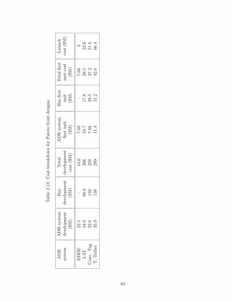
Tab
le2.
13:
Cos
tbre
akdow
nfo
rP
aret
ofr
ont
des
igns.
AD
Rsy
stem
AD
Rsy
stem
dev
elop
men
t($
M)
Bus
dev
elop
men
t($
M)
Tot
aldev
elop
men
tco
st($
M)
AD
Rsy
stem
firs
tunit
($M
)
Bus
firs
tunit
($M
)
Tot
alfirs
tunit
cost
($M
)
Lau
nch
cost
($M
)
ED
DE
22.5
-44
.67.
68-
7.68
3L
AT
34.0
86.8
206
10.7
17.8
28.5
22.6
Con
v.
Tug
22.6
132
258
7.68
29.5
37.2
51.8
T.
Tet
her
35.9
138
289
11.4
31.2
42.6
66.4
65
2.3.2 Orbital Scrapyard Scenario
An alternative orbital scrapyard scenario was considered in an attempt to
mitigate the risk posed by uncontrolled reentry of debris removed by the orbital
tugs. In this scenario, each orbital tug moves all DOs to a single orbital scrapyard.
This scrapyard was positioned in a circular orbit at an altitude of 600 km and with
an inclination of 74deg, with its right ascension centered within the band of orbits
of the target DOs for that vehicle. Relative nodal precession between this scrapyard
and the DOs was not considered. It was assumed that the orbit for the scrapyard
was selected to minimize the risk of collision with other spacecraft and debris, while
remaining easily accessible from the simulated debris belt. Use of this alternative
methodology was assumed to reduce the trajectory risk of low thrust orbital tugs
from high risk to medium risk, since an uncontrolled reentry no longer occurs. RL
and RH were therefore set to 0 for low thrust tugs. Orbital scrapyards are an
untested mission architecture, with no known proof of concept having flown at the
time of this writing. Therefore, in this scenario, the ADR system of any low-thrust
tug is assumed to be TRL 2.
The results of this scrapyard scenario are given in Table 2.14 and Fig. 12. In
this scenario, EDDE appears to have increased in cost, while decreasing in ORF .
The plane change required for EDDE to move DOs to the plane of the scrapyard
now dominates time per object required. As a result, a larger fleet of vehicles is
required to meet the required removal rate of 10 objects per year, raising the cost
per DO removed for EDDE. The decrease in EDDEs overall risk factor is due to the
66

elimination of uncontrolled reentries for DOs, as well as crossings of high priority
orbits. As a result, EDDE now has an expected cost overrun of $34M and schedule
slippage of 13.5 years. While the overall TRL of EDDE has decreased, substantially
increasing RTRL, ORF has decreased due to a near elimination of the RT in this
scenario. The LAT has increased in cost in this scenario, though not profoundly.
Unlike EDDE, ORF has actually increased for the LAT in this scenario. The LAT
spacecraft utilizes conventional subsystems with the exception of the ADR system.
As a result, it suffers from a greater change in TRL between scenarios than EDDE,
leading to ORF increasing. Like EDDE, the LAT now requires a larger fleet size
to meet the DO removal rate requirement due to the large plane change required.
This is almost exclusively responsible for the cost increase of the LAT. Terminator
Tether was unaffected, since as a DP, its concept of operations was unchanged in
this scenario.
67

Tab
le2.
14:
Cos
tbre
akdow
nfo
rP
aret
ofr
ont
des
igns,
Orb
ital
Scr
apya
rdSce
nar
io.
AD
Rsy
stem
AD
Rsy
stem
dev
elop
men
t($
M)
Bus
dev
elop
men
t($
M)
Tot
aldev
elop
men
tco
st($
M)
AD
Rsy
stem
firs
tunit
($M
)
Bus
firs
tunit
($M
)
Tot
alfirs
tunit
cost
($M
)
Lau
nch
cost
($M
)
ED
DE
EB
14B
BB
AA
O-
--
80kg
82kg
191
day
sL
AT
HB
7A
BB
AB
E10
0kg
115
kg
200
kg
290
kg
710
kg
580
day
sT
.T
ether
GF
20A
AA
BB
P10
0kg
3200
kg
370
kg
1500
kg
5200
kg
4day
sC
onv.
Tug
BE
4A
AA
BB
C80
kg
2800
kg
340
kg
190
kg
3400
kg
4day
s
68
2.3.3 Additional Options
No aerodynamic drag based designs appeared on the Pareto front, even in
the case where deorbit is performed at solar max. These designs did appear in the
results, however both r and financial cost were higher than that of the conventional
tug. It is possible that the cost of these systems as well as that of Terminator Tether
could be lowered such that they are competitive with the remaining designs on the
front by attaching their DPs to launch vehicle upper stages and spacecraft prior to
launch. The DP could then be used as a simple, propellantless deorbit device at end
of life for a spacecraft or after completing orbital delivery for spent upper stages.
Treating a DP as a scientific instrument and applying the Spacecraft/Vehicle Level
Cost Model, the development and first unit production costs are given in Table 2.15.
Assuming a Terminator Tether design as described in this paper is used for 100 deor-
bits, with the development cost spread evenly across all DOs deorbited, and applying
an 80 percent learning curve, on average such a device will cost $1.4M per launch.
Assuming $8,000 per kg for launch on a Kosmos 3M [46], the rocket whose upper
stages are used as model DOs in this analysis, the portion of the rockets payload
lost to the DP would be approximately $225,000 in value. Therefore, this method of
DO deorbit can be assessed at a cost of approximately $1.6M per DO. As discussed
earlier, the ADR specific risk and destructive collision cross section ratio are both
minimized for Terminator Tether. Since the device would only have to remain on
orbit for the duration required to deorbit a single DO, the required lifetime would
not be a concern with regard to risk factors, as defined here. Therefore, attaching
69

Figure 2.12: Leading vehicle designs assuming use of orbital scrapyards.
70

a DP prior to launch would provide an ADR method with costs competitive with
EDDE, at substantially lower risk.
Table 2.15: DP development and first unit costs.
ADRsystem
Developmentcost ($M)
First unitcost ($M)
KSII 22 7.3TRIS 26 9.3
GOLD 21 7.0Terminator Tether 13 3.7
2.3.4 1D Cost Function Evaluations
In an attempt to achieve a clear ranking of Pareto-optimal vehicle designs, a
comparison was performed by using a cost adjusted by r as a single, one-dimensional
figure of merit. This adjusted cost per object ca was determined as indicated in Eq.
2.7:
ca = CDO +r
Ncsat (2.7)
In essence this adjusted cost assumes that a debris removal program, if implemented,
must pay for any damages resulting from debris removal operations in addition to
other program costs. The fitness function was changed to
fr =1
ca(2.8)
and all scenarios were re-evaluated using this new fitness function. The results of
these runs are given in Fig. 2.13, Fig. 2.14, and Fig. 2.15.
71

Figure 2.13: Leading Vehicle Designs - Baseline Scenario - Adjusted Cost
72

Figure 2.14: Leading Vehicle Designs - Solar Max Scenario - Adjusted Cost
73

Figure 2.15: Leading vehicle designs assuming use of orbital scrapyards(adjusted cost).
74

The designs listed in these figures bear a strong resemblance to those in Fig. 2.10,
Fig. 2.11, and Fig. 2.12. A list was produced, ranking designs byca. The lists for
all three scenarios were combined, with the results presented in Table 2.16. Designs
that are in the same group of the Pareto front, such as all of the LAT designs in Fig.
2.13, are assumed to be variations of the same vehicle design, and therefore only
the design with the lowest adjusted cost in each group is presented in Table 2.16.
Groups of designs have also been combined from Fig. 2.13 and Fig. 2.14, since, as
with the original cost function, no aerodynamic decelerators appeared on the front
in either scenario, and therefore the difference in the two scenarios is not expected
to have an influence on vehicle designs.
All designs listed in Table 2.16 have an adjusted cost within a factor of no
more than 1.75 of each other. Due to the uncertainty in the exact relationship
of risk and cost, all of the designs presented in the table should be considered of
equal merit. All warrant further investigation moving forward, likely making a final
decision using additional criteria not considered in this work.
75

Tab
le2.
16:
Lea
din
gve
hic
ledes
igns
bas
edon
adju
sted
cost
.
Gen
ome
AD
Rsy
stem
Sce
nar
ioT
otal
mas
sT
ime
per
DO
rem
oved
ORF
Cos
tp
erD
Ore
mov
ed
Adju
sted
cost
per
DO
rem
oved
GF
20A
AA
BB
KT
.T
ether
Scr
apya
rd52
00kg
4day
s0.
25$1
2.5M
$14.
1MH
S17
BB
BA
AC
LA
TSta
ndar
d/S
olar
Max
490
kg
419
day
s1.
4$7
.0M
$16.
3ME
Y13
BB
BA
BD
ED
DE
Scr
apya
rd81
kg
173
day
s2.
4$1
.1M
$17.
4ME
Q1
BB
BB
Ae
ED
DE
Sta
ndar
d/S
olar
Max
85kg
4day
s2.
4$6
.4M
$22.
4ME
i28
BB
BA
Aq
ED
DE
Sta
ndar
d/S
olar
Max
87kg
32day
s3.
3$0
.82M
$23.
3MH
E7
AB
BA
BB
LA
TScr
apya
rd59
0kg
533
day
s2.
4$8
.3M
$24.
4M
76

2.4 Summary
The current debris population in low Earth orbit has reached a point where,
even with no new satellite launches, it will grow due to collisions between existing
on orbit objects. The present work detailed an investigation of leading designs un-
der consideration for orbit based removal of low Earth orbit debris. Designs were
evaluated in three scenarios; a standard scenario, where all DOs are deorbited, a
solar max scenario, where aerodynamic decelerators are reduced in mass under the
assumption that debris removal occurs at solar max, and an orbital scrapyard sce-
nario, where low thrust tugs gather all DOs in a scrapyard rather than directly
deorbiting them. Designs in each scenario were evaluated based on their financial
cost per object removed and a programmatic risk factor. In each scenario, Termi-
nator Tether, LAT, and EDDE designs appeared on the final Pareto front, with
each grouping of Pareto-optimal designs within the design space based around one
of these technologies. The conventional tug exhibited very similar performance to
Terminator Tether, although it did not actually appear on the front. However, due
to the conventional tugs proximity to the front, its performance is considered es-
sentially equal to Terminator Tether within the scope of this study, and therefore it
warrants further investigation.
The benefit of propellantless vehicle designs (the LAT and EDDE) is evident
from this study, with all but the most expensive Pareto-optimal programs being
designed around such technologies. The fact that these vehicles need not carry all
propellant for their mission at launch allows them to remove a large number of DOs
77

without becoming prohibitively massive. Additionally, of the designs on the front
that utilized a dedicated propulsion system, none used a high Isp electric propulsion
system. This is due to the larger fleet size that would be required as a result of the
large time per DO resulting from the low thrust nature of these systems.
The absence of aerodynamic decelerator based designs on the Pareto front
indicates that these devices are currently of too great of a mass to achieve comparable
performance to the Pareto-optimal designs. Not only must these vehicles carry all
mission required propellant at launch, but they must also carry a number of DPs
equal to the number of DOs they are to remove. In all aerodynamic decelerator
cases, this mass, combined with the production costs of the DPs, raised the cost per
DO for each of these systems substantially beyond that of Terminator Tether and
the conventional tug. These methods of debris removal may still prove beneficial if
attached to satellites and launch vehicle upper stages prior to launch. The system
could then passively deorbit an upper stage without the expense and complication
of sending a dedicated ADR vehicle. Further investigation should be performed to
refine this option, and to determine under what conditions it may be the preferred
method of debris removal.
Based on the above work, the Electro-Dynamic Debris Eliminator, the Laser
Ablation Tug, a passive electrodynamic drag tether such as Terminator Tether,
and a conventional tug utilizing an impulsive chemical propulsion system should be
considered for further analysis. Additionally, other passive decelerator technologies,
while not as high performance as the aforementioned systems when delivered by
space based systems, may be useful for deorbiting future orbital objects (satellites
78
and launch vehicle upper stages) if attached before launch. The final design that
should be developed for debris removal will depend on the results of this future
analysis. In addition, the risks to people and infrastructure, both on orbit and on
the Earth, must be weighed with the added financial burden of a lower risk system,
and a decision made as to what level of risk is acceptable to avert the impending
risk of an ablation cascade.
79
Chapter 3: The General Static CR Model
3.1 Overview
This chapter lays out the basic form of the CR model, around which remain-
der the framework is built. This form of the model addresses systems where all
components are assumed to be in a steady state. In these systems resource flows
are constant. It is therefore sufficient to analyze such a system at a single point in
time.
The static CR model is not sufficient to model most spacecraft, where com-
ponent behavior changes over time. However, it is beneficial to introduce as many
concepts of the CR model and framework as possible in the context of a static design
problem. The design of a lighting system is used as an example in this chapter to
help describe the static CR model. Later chapters will detail the necessary additions
to extend the framework to dynamic problems like spacecraft design.
3.2 Component Definition
As has been stated, the CR model takes a complex system and models it as a
collection of components and resources flowing between them. Each component may
80
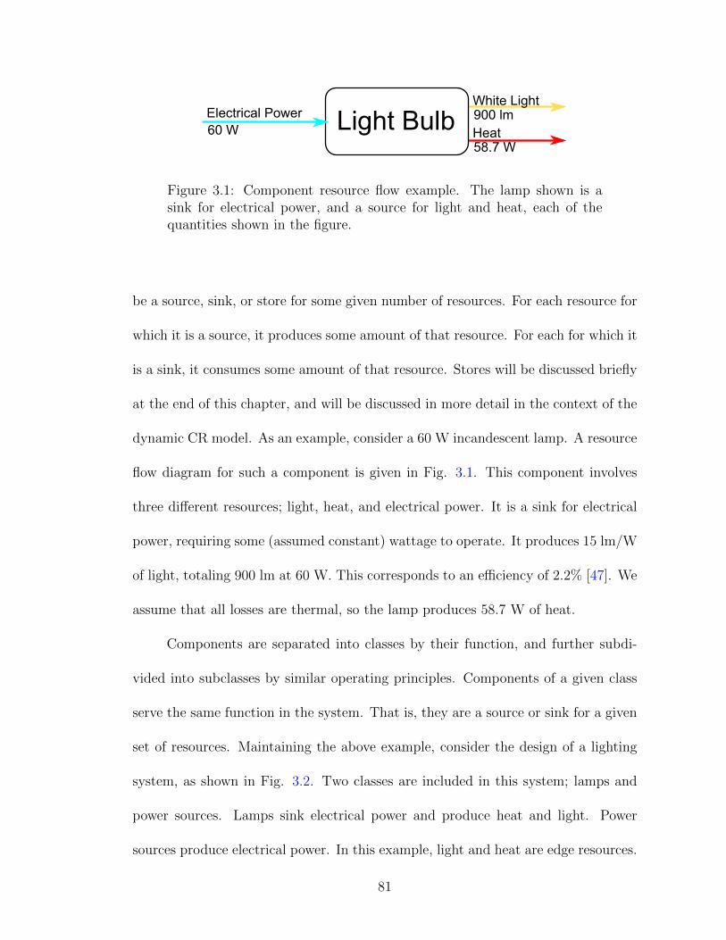
Light BulbElectrical Power
60 W
White Light900 lm
Heat58.7 W
Figure 3.1: Component resource flow example. The lamp shown is asink for electrical power, and a source for light and heat, each of thequantities shown in the figure.
be a source, sink, or store for some given number of resources. For each resource for
which it is a source, it produces some amount of that resource. For each for which it
is a sink, it consumes some amount of that resource. Stores will be discussed briefly
at the end of this chapter, and will be discussed in more detail in the context of the
dynamic CR model. As an example, consider a 60 W incandescent lamp. A resource
flow diagram for such a component is given in Fig. 3.1. This component involves
three different resources; light, heat, and electrical power. It is a sink for electrical
power, requiring some (assumed constant) wattage to operate. It produces 15 lm/W
of light, totaling 900 lm at 60 W. This corresponds to an efficiency of 2.2% [47]. We
assume that all losses are thermal, so the lamp produces 58.7 W of heat.
Components are separated into classes by their function, and further subdi-
vided into subclasses by similar operating principles. Components of a given class
serve the same function in the system. That is, they are a source or sink for a given
set of resources. Maintaining the above example, consider the design of a lighting
system, as shown in Fig. 3.2. Two classes are included in this system; lamps and
power sources. Lamps sink electrical power and produce heat and light. Power
sources produce electrical power. In this example, light and heat are edge resources.
81

Lamp
Electrical Power
LightHeat
System
Environment
Figure 3.2: Lighting system example. This simple example contains twotop-level component classes; lamps and power sources.
Each component class can contain multiple subclasses. Components within a
given class are grouped into subclasses by similar manner of operation. Doing so
allows a similar component-level model to be used for all components of a subclass,
only changing the values of variables in the model. In this example, incandescent
lamps, fluorescent lamps, and LED lamps may each be their own subclass of the
lamp class.
The resource flow for the incandescent lamp subclass would then be defined
in equations 3.1, 3.2, and 3.3:
Pin = Pop[W] (3.1)
Lout = λlmPin[lm] (3.2)
Hout = (1− ηlamp)Pin[W] (3.3)
82

where Pin is the power consumed, Pop is the required operating power of the com-
ponent in W, Lout is the light produced, λlm is a conversion factor from electrical
power to light, Hout is the heat produced, and ηlamp is the efficiency of the lamp.
Maintaining the assumption that all energy entering the lamp is converted to either
light or heat, it is possible to equate λlm and ηlamp, but they will both be kept as sep-
arate properties for simplicity of the example. Pin, Lout, and Hout are the resource
flows to and from the component. The goal of the component class (and subclasses,
where applicable) is to determine the resource flows of the component as functions
of the remaining properties. The values of these component parameters are defined
for each specific component. The component parameters for all components of a
given subclass are compiled into a component library for that subclass.
Component parameters can either be fixed, appearing as a constant for each
entry in the library, or genetically determined, in which case the range of possible
values is described in the component library. Allowing for components with geneti-
cally determined parameters gives the framework the ability to handle some design
aspects of individual components. This distinction enables the framework to propose
and optimize its own components for subclasses in which component behavior can
be analytically described. It is envisioned (and is certainly the case in the spacecraft
design problems of interest to the author) that systems may exist that contain “off
the shelf” components, which will henceforth be referred to as “real” components.
However, the ability to propose new or custom components may be desirable. These
will henceforth be referred to as “notional” components.
83

This is indeed the situation in current practice integrated space mission design.
Previously flown components are used where possible, and where they efficiently ful-
fill a given role, but new components are also developed for a new spacecraft. At this
proposal-level mission design, novel components are often modeled by interpolation
and regression of data from existing components, as well as with analytical models.
The goal of variable component parameters is to allow the CR model to handle and
replicate this capability.
As an example, consider a high gain parabolic antenna (HGA) for a spacecraft.
The gain of the antenna is defined as
G = 10Log10
(4πeAA
λ2
)[dBi] (3.4)
where eA is the antenna efficiency, A is the aperture area of the antenna in m2, and
λ is the wavelength of the transmitted signal in m. The mass of the antenna is
defined as
m = ρA[kg] (3.5)
where ρ is the areal density of the antenna, in kg/m2. The values of eA and ρ will
be a function of the antenna material and construction, accounting for factors that
cannot be modeled analytically in a simple way. λ is determined by the incoming
signal from the spacecraft’s transmitter, which would be considered a resource for
which an antenna of this class is a sink. A is defined by the designer, and drives the
gain and mass properties given eqs. 3.4 and 3.5. An entry in the component library
84
for notional parabolic antennas would then contain constant component parameters
for eA and ρ, and the range of reasonable values for A, or more likely, r, defining
A = πr2. r would then be determined by a component genome, discussed in more
detail in Chap. 4.
To summarize, all components within a given class or subclass exist as a list-
ing of parameters in the component library for that class or subclass. The class
or subclass then models the resource flows of the component as a function of its
component parameters. These resource flows then describe the interactions of the
component with the rest of the system. Fig. 3.1 illustrates the calculated resource
flows for a component with Pop = 60 W, λlm = 15 lm/W, and ηlamp = 0.022, based
on [47]. By constructing a system from combinations of components and analyzing
the resource flows between them, the CR model is able to determine the behavior,
performance, and feasibility of the system as a whole.
3.3 Resource Analysis
Following the procedure from the previous section, one is left with a series of
components, each producing and consuming known quantities of given resources.
Analysis of these resource flows between components serves as the system-level sim-
ulation for the CR model. This ultimately leads to an ability to assess the per-
formance and feasibility of whole systems, allowing generalized analysis of multiple
design options for a given design problem.
85

Two types of resources exist within the CR model; internal resources and edge
resources. Internal resources flow between components of the system, and must
be balanced, as described below. Edge resources flow between the system and its
external environment. In the static CR model, edge sources can supply a resource
flow into the system at a constant rate, and edge sinks can consume some flow
produced by the system at a constant rate. Either of these rates may be finite or
infinite by convention. In the case of infinite edge resources, the amount of a given
resource flowing to or from the environment is tracked. These tracked values may
then serve as figures of merit for determining the performance of the system. In
our lighting system example, objectives may be to maximize the amount of light
produced and minimize the heat produced by the system. Light and heat are edge
sinks, produced within the system and sunk to the external environment. It is
not a requirement that edge resources are the only figures of merit in the design
problem. Additional objectives in this design problem may be to minimize the mass
or minimize the financial cost of the system.
The power of the CR model is that constraints can be naturally handled
through resource flows. The net flow of each resource is constrained to be greater or
less than some constant value. In most cases this constant ends up being zero. That
is, a resource is constrained simply to have a surplus or deficit across the system.
For the lighting system, the driving feasibility constraint is that the power sources
produce at least as much electrical power as the lamps consume.
Usually an objective value is determined by summing the value of a given
property across the system. For non-resource figures of merit such as mass and
86

cost, this is straightforward. Property values are directly summed across all system
components. For resource tabulation, the process is a little more involved. For a
given design problem, a resource relation
δi = Σi,source − Σi,sink (3.6)
is defined for each resource i, where Σi,source is the total amount of resource i pro-
duced across all components of the system, and Σi,sink is the total amount of resource
i consumed across all components of the system. For each resource, δi is constrained
to be greater than or less than some constant, often zero. This implies a desired
surplus (for δi > 0), or deficit (for δi < 0) of a given resource. This concept is then
the heart of the CR model.
A complex system can be decomposed into a series of components, each of
which produce and consume certain resources at a given rate. Most constraints on
the system can be handled by balancing this resource flow across the system. In the
lighting system example there is only a single internal resource - electrical power. As
discussed above, we wish to constrain the problem, ensuring that at least as much
electrical power is available as is consumed within the system. Therefore,
δP > 0, (3.7)
where δP is the resource relation for electrical power within our system.
87
The final topic to discuss regarding resources in the static CR model is the
concept of resource conditioning. A resource may have properties associated with it
besides its flow rate. As a result, multiple versions of the same resource may exist
within the system. In our example problem, voltage may serve as a condition on
electrical power flow. It is possible to have a power source that produces power
at one voltage, and a lamp that requires power to be supplied at another voltage.
For all intents and purposes, flows of the same resource with different conditioning
function as separate resources altogether. Resource conditioning serves as an added
layer of complexity that may or may not be necessary for analysis, depending on
the problem at hand.
The main purpose in organizing resources in this way is to facilitate compat-
ibility checking between sources and sinks of a given resource within the system.
Versions of the same resource with different conditioning can simply be summed
to a single value, ignoring any compatibility issues at this stage of analysis. Alter-
natively, they can be treated as completely separate resources, or some conversion
penalty can be imposed to convert from one conditioning to another. In the case of
the former, additional components could be added to the system that perform con-
version. For example, a transformer can be added to convert from power produced
at one voltage to power consumed at another voltage.
88

3.4 The Quasi-Static CR Model
One extension to make to the static CR model is to introduce components
with stores, as alluded to earlier, to the model. A store is a type of component that
contains a finite internal reservoir to cache a particular resource. A store operates
as either a source or sink, depending on other resource flows within the system.
In the lighting system problem, a possible example would be to express batteries
as a subclass of power sources. A battery starts fully charged (that is, with its
electrical power reservoir full). It operates as a source, providing electrical power
to other components within the system. One common use of stores is to handle
component lifetime constraints, especially when those lifetimes may be tied to some
other resource flow. For example, a lamp may only be able to produce some amount
of light before it is expended. In this case, the lamp can be considered a store for
component lifetime, which depletes at some rate per light produced.
The model is no longer truly static, since resource relation violations may
occur when stores are depleted. The model is still quasi-static, with the system
still operating in steady state until a store is depleted or filled. This implies the
resource flow of the system does not change during operation, so stores operate as
either a source or a sink, but never both in the same simulation. Assuming stores
are utilized, they will at some point be either expended (if operating as a source) or
completely filled. At this point, they no longer function as a store for that resource
in the system. The elapsed time at which this happens is tracked, and the resource
flow of the system subsequently changes. If any resource relations are violated as
89
a result, the simulation ceases, with the total simulation time elapsed noted. This
simulation time then becomes a figure of merit, which may be used as an objective,
or as an input to some more complicated objective function.
It may be evident at this point that there is a potential for modeling more
complicated systems with time varying resource flow, due to operational changes or
environmental changes external to the system. In such cases, stores may operate
as either sources or sinks at different points in time depending on the state of the
rest of the system. In the lighting system example, a battery may provide power
from its internal reservoir until power is expended, but may then be recharged by
an external power source, which, if necessary, may power other components of the
system simultaneously. Most of the problems of interest to the author are of this
more complex, dynamic nature. They will be addressed in full detail in the following
sections on the General Dynamic CR model.
90

Chapter 4: Optimization with the CR Model
4.1 Overview
The motivation behind the CR model is to facilitate automated design opti-
mization of a wide class of complex systems built from discrete components in a
very uniform manner. The CR optimization problem can be generally stated as
min F (C,x)
s.t. δi ≥ ki
δj ≤ lj
∀i ∈ 1, ...,M,
j ∈ 1, ..., N
(4.1)
where each δi is a surplus constraint and each δj is a deficit constraint, and ki and lj
are a series of constants. For surplus constraints, the requirement is that more of the
resource associated with that relation is produced than consumed across the system.
For deficit constraints, the opposite is true. M and N are the total number of surplus
and deficit constraints, respectively. C is the set of all components comprising an
individual design, and x is the vector of system-level variables beyond component
91

selection. F (C,x) is the objective function, which varies with the specific design
problem. In words, the problem can be stated as follows: find the combination
of allowable components and system-level design variables that optimize objective
performance while meeting all required resource flows, ensuring proper functioning
of the system.
A specialized GA detailed in this chapter, was developed to perform this op-
timization. A GA was selected for its ability to perform more complete design
space exploration simultaneously compared to other metaheuristic optimization al-
gorithms. This is due to the way it produces entire generations of design options
spanning a trade space. The penalties for increasingly large numbers of variables
are also much lower for GAs than many other optimization techniques. This makes
them well-suited for problems with a large or variable number of design parame-
ters. As was discussed in the introduction, substantial literature already exists for
handling variable-size problems with GAs.
Metaheuristic algorithms do not rely on any analytical knowledge of the prob-
lem for optimization. This makes them well suited for multidisciplinary problems.
In these problems, the relationship between the design variables and objective func-
tions is complex, and may be iterative or even transcendental. GAs in particular
are well-suited for combinatorial problems with discrete variables, like component
selection problems [19]. Furthermore, there is an extensive history of applications
of GAs for multiobjective design space exploration problems [19,21,48,49], the role
this work seeks to fill.
92

An overview of GAs in general can be found in Chap. 1. The remainder of this
section will focus on the particulars of the GA implementation developed for this
dissertation. Unlike most other GAs, this implementation utilizes a variable length
genome. Each gene of the primary genome corresponds to a component present
in the system. Enabling the genome length to vary across population members
and from parent to child allows the algorithm to naturally vary the number of
components in a design.
4.2 The VEGA Genome
A variable length chromosome is utilized to maintain the greatest generality
possible. It naturally allows the number of components present in a system design
to vary within a given design problem. The VEGA genome is separated into three
levels, summarized in Table 4.1, with a simplified satellite genome example given in
Fig. 4.1:
Table 4.1: Various levels of the VEGA genome.
Genome level Description
0 System-level genes1 Primary genome/component selection genome2 Component-level genome
The Level 1 (L1) genome, or system-level genome, accounts for problem-
specific design parameters. These parameters cannot be tied to a given component.
They drive the behavior of the system as a whole. For example, consider a spacecraft
93

Thrusters 3 10 2 9 6
Level 2 Genome
Level 1 Genome
19.0 139.96731 0 51.6
a e i
Electrical
Power 1 8 9 9 1 4 3 9 5 10
C&DH 2 3 2
Notional
HGA 3 6
Real
Omni 3 7 3 4
...
r = 0.6
Level 3 Genome
Figure 4.1: Simplified genome for a spacecraft design. The L1 genomespecifies the orbit in which the spacecraft will operate. The L2 genomespecifies the components that comprise the spacecraft, and is separatedinto chromosomes based on component class. The final chromosomedisplayed is for notional HGAs, described to some extent in Chap. 2.For one of these, the L3 genome is displayed, specifying the radius of theantenna.
94

design. The orbit in which a spacecraft is operating has a strong influence on its
performance and requirements. Several orbit options may be available for a given
mission. This may consist of a number of discrete orbits. Alternatively, the orbital
parameters may exist as continuous variables to be optimized in the design problem.
In both cases, the orbit would be determined using genes in the L1 genome.
The goal of VEGA is to support a system design optimization framework
that is as general as possible. Contrary to this, the L1 genome is very problem
specific. Much of the purpose of the L1 genome is to encapsulate any necessary
design variables specific to the problem at hand, passing them to the simulation.
Therefore, for a specific design problem, the user must specify the sequence of L1
genes. Some additional information about each gene, based on whether it is discrete,
or continuous is also required. For discrete genes, the user can either specify a list
of all possible values, or a range within which any integer value is acceptable. For
continuous genes, the user simply specifies the bounds for possible values. Then, for
a given individual, the L1 genome will then be passed with the system object to the
system-level simulation.
The Level 2 (L2) genome is the most critical portion of the genome, and is
always included. It dictates which components are present for a given individual.
The L2 genome is segmented into “chromosomes” by component class and subclass.
Crossover is then performed separately between corresponding chromosomes. The
reason for this segmentation is related to how the variable length crossover operator
functions. Its purpose will become evident in that section. Within each chromosome,
the value of each individual gene references a component in the component library
95
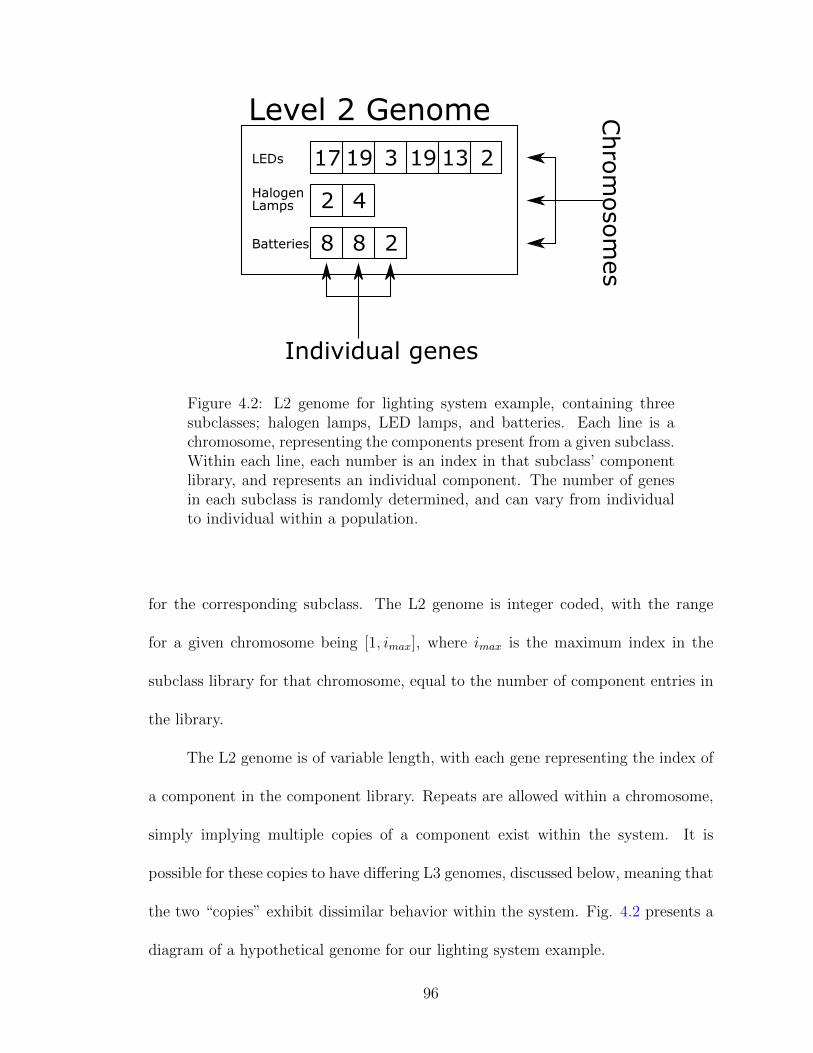
LEDs 17 19 3 19 13 2
HalogenLamps 2 4
Batteries 8 8 2
Level 2 Genome Chro
mosom
es
Individual genes
Figure 4.2: L2 genome for lighting system example, containing threesubclasses; halogen lamps, LED lamps, and batteries. Each line is achromosome, representing the components present from a given subclass.Within each line, each number is an index in that subclass’ componentlibrary, and represents an individual component. The number of genesin each subclass is randomly determined, and can vary from individualto individual within a population.
for the corresponding subclass. The L2 genome is integer coded, with the range
for a given chromosome being [1, imax], where imax is the maximum index in the
subclass library for that chromosome, equal to the number of component entries in
the library.
The L2 genome is of variable length, with each gene representing the index of
a component in the component library. Repeats are allowed within a chromosome,
simply implying multiple copies of a component exist within the system. It is
possible for these copies to have differing L3 genomes, discussed below, meaning that
the two “copies” exhibit dissimilar behavior within the system. Fig. 4.2 presents a
diagram of a hypothetical genome for our lighting system example.
96

In order to initialize the first generation of designs for an optimization run, it is
necessary to randomly determine all chromosomes of the L2 genome. This involves
randomly determining both the number of components and selection of components
present. The latter is straightforward once the former is accomplished. For the
former, a set range on the number of components in each class is used to generate
the initial population. By default, the range on number of components for a given
subclass is [0, 10], but this starting range can be user defined as well. As will be
discussed, this is simply used to bound the genome size of the initial population,
and has little bearing on the final chromosome length to which the GA converges.
The final remaining portion of the genome is the Level 3 (L3) or component-
specific genome. The L3 genome exists to support notional component subclasses,
where component behavior is a function of some number of selectable options for
a given component. For notional components, analytic relations exist for defining
components as a function of some number of parameters. The encoding of L3 genes
is therefore specific to each component class which utilizes them. It is implicitly
defined through the component class model on a case-by-case basis.
L3 genes are created when a component is first initialized. This usually occurs
when randomly generating the first generation of designs. The values of the L3
genes for the given component are randomly determined as well. The component is
essentially “fixed” at this point, maintaining the same L3 genome as it is inherited
from generation to generation. There is still the potential for the L3 genes to
mutate each time the component is inherited. Therefore, it is still possible that an
L3 genome may vary over the multiple generations of an optimization run.
97

4.3 The Variable Length Crossover Operator
Considerable effort in the development of this GA entailed the design of the
variable length crossover operator, which allows the GA to vary and optimize the
number of components included in a system as part of its regular iteration. This
section is therefore included, and focuses solely on the discussion of that effort. The
overall operation of our GA implementation will be detailed in the following section.
In order to utilize a GA with a variable length genome, special considerations
must be made in the algorithm’s crossover operator. The crossover operator devel-
oped for this work draws heavily from that proposed by Ting et al. [25]. It is largely
what Ryerkerk et al. refer to as a cut and splice crossover [15], but includes some
design philosophies of their synapsing variable length crossover. In the latter, the
genome is grouped or “synapsed” by identifying common substrings in both parents,
aligning those, and then performing n-point crossover, with the crossovers inserted
within the synapsed portions of the genomes.
The encoding scheme for VEGA presents a straightforward method for a pro-
cess similar to synapsing the genome - grouping it by chromosomes. The genome is
in fact already grouped into chromosomes in this way. VEGA matches correspond-
ing chromosomes of the L2 genome from each parent, then performs a cut and splice
crossover for each chromosome. The cut and splice crossover operates in essentially
the same way as an n-point crossover. The difference is that, rather than inserting
the crossover points at the same random location in both parent genomes, they are
inserted at different random locations in each parent genome. This is illustrated in
98

A B C D E F G
a b c d e f g
Parent 1
Parent 2
A
B C D E F G
d e
ba c
fChild 1
Child 2 g
Figure 4.3: Cut and splice crossover. The example provided here is fora two-point cut and splice crossover. Note how this operator varies thechromosome length.
Fig. 4.3. Each child inherits genes from the corresponding parent (Child 1 from
Parent 1, Child 2 from Parent 2) until a crossover point is reached on each parent
genome. Both children then flip, inheriting genes from the other parent, continu-
ing this process, flipping between parents at each crossover point until all genes in
both parent chromosomes has been assigned to the child genomes. For VEGA, a
single-point cut and splice crossover is used for each chromosome.
A similar component crossover (SCC), also proposed by Ryerkerk et al. [15],
was considered. The concept of SCC is to find pairs of similar components between
the parent genomes. That is, components which serve the same role in their respec-
tive designs. Each component in one parent genome is compared to each component
in the other parent genome. Each pair is assigned a similarity, or, in the case of [15],
a dissimilarity. Ryerkerk et al. defined this dissimilarity as
D =1
n
n∑i=1
|C1i − C2i|σi
(4.2)
99
where C1i and C2i are the values of the ith parameter of the two components being
compared, σi is the standard deviation in the ith parameter over the entire popula-
tion, and n is the number of parameters. Some threshold of dissimilarity is defined,
0.5 in the case of [15]. Any component pairs with a dissimilarity less than this value
are considered similar. Once the dissimilarity between all components has been
calculated, the most similar pair is placed in the genome. The next most similar
pair of the remaining components is then placed in the genome, and this process
repeats until the threshold of dissimilarity is reached. The genome up to this point
is of fixed length, since only pairs of components from each parent have been added.
The remaining components (the dissimilar components) are added to the genomes
of their respective parents as is. A standard n-point crossover is then performed on
the similar portions of the genomes, and a cut and splice crossover is performed on
the dissimilar portions of the genomes.
The similar component crossover developed for VEGA was inspired by this one,
but operates somewhat differently. The similarity evaluation is somewhat more in-
volved than that outlined above. This was necessary due to differences in the genome
encoding scheme. Usually (except in the case of notional components), there is only
a single parameter in the genome for each component. That parameter is simply a
reference to an index in a component library. The measure of functional similarity
in the CR model is the extent to which two components’ resource flows are the same.
For VEGA, a value for similarity was determined, rather than dissimilarity. This
similarity was defined through the following derivation. Let the resource similarity
100

be defined as
Sji = min
[rjiArjiB
,rjiBrjiA
](4.3)
where Sji is the similarity of the ith resource present in the two components, with
either j = I, implying this is a resource flowing into the component (a resource for
which the component is a sink), or j = O, implying this is a resource flowing out of
the component (a resource for which the component is a source). rjiA and rjiB are the
corresponding resource flows of the components being compared. Expressing Sji in
this way means that its value will always be between 0 and 1, with 0 implying the
resource flow is only present on one of the two components (completely dissimilar)
and 1 implying the same flow of that resource on both components (completely
similar). The similarity of all resource flows present in the components is then
averaged to determine the overall source and sink similarities for the pairs:
Sj =n∑i=1
Sjin
(4.4)
Finally, the overall similarity is defined as the average of the overall source similarity
and overall sink similarity:
S =SO + SI
2(4.5)
S is determined for each pair of components within a given chromosome of the
two parent designs. The threshold of similarity was defined as 0.5. Any components
with similarity greater than this threshold that are considered similar. As in [15],
pairs of components are added to the similar portion of the genome until the highest
101

similarity of remaining possible pairs is less than the threshold value. Crossover is
then performed in the same manner as in [15].
Ultimately, SCC was not adopted for VEGA, which continued to use the simple
cut and splice crossover, based on performance with a preliminary test scenario.
The design problem of this test case was to design a table to hold a given payload
mass. This problem will be discussed in full detail in the next chapter. The specific
reason for this abandonment is that SCC and cut and splice were found to produce
comparable results, but SCC required much higher computation time to achieve
these results. This additional computation time was required to calculate S for
each pair of components for each pair of parents during recombination, a problem
which is O(mn2n) (this is actually slightly pessimistic, due to similarities only having
to be calculated by chromosome, but is still of the right order). In the table test
problem, designs in the initial generation had an average of 16-18 components, with
an average of two resources per component, requiring approximately 600 resource
similarity evaluations per set of parents. The problem used a generation population
size of 500. 30% elitism was used, “cloning” the 150 most fit population members to
the next generation. The remaining genomes for each new generation were produced
through genetic crossover, requiring 175 pairs of parents to produce 175 pairs of
children. As a result, approximately 150,000 resource similarity evaluations were
required for each new generation.
After substantial optimization of the SCC, the GA still took three times as long
to run as when using the cut and splice crossover. Fig. 4.4 shows the performance
of the GA using the cut and splice crossover. Fig. 4.5 shows the performance of the
102

Figure 4.4: VEGA performance using cut and splice crossover.
GA using the SCC, which has been superimposed on the results from Fig. 4.4. As
can be seen, the cut and splice operator did not produce substantially better results.
Additionally, this was for a fairly simple test case, with most designs in the initial
population containing less than twenty components. For a more complex problem
like spacecraft design, the number of components per design would be expected to
be substantially larger. An increase in the number of components corresponds to
a quadratic increase in the number of resource similarity evaluations. For these
reasons, similar component crossover was not developed beyond this point, and
the cut and splice crossover has been used for all following VEGA optimizations
presented in this work. Sometimes the simplest solution is the correct one.
103

Figure 4.5: VEGA performance using similar component crossover. Forcomparison, the results from Fig. 4.4 are superimposed, faded, on thisplot.
4.4 VEGA Operation
The general operating process of VEGA is the same as that of a traditional
GA, as depicted in Fig. 1.1, repeated here as Fig. 4.6 for reference. The algorithm
begins by randomly generating the initial population. The fitness of each individual
in the population is evaluated as a combination of user-specified objectives. A
new generation is produced from the current one through genetic selection variable
length crossover, and possible mutation. The process then repeats starting again
with fitness evaluation for the entire generation, iterating successive generations
until some stopping condition is reached. The remainder of this section will discuss
each of these steps in detail.
104

Generate initial random population
Selection (select two parents)
Recombination
New generation filled?
No
Yes
YesNew Generation No
Figure 4.6: Genetic algorithm process. The algorithm is initialized witha population of random individuals. For each generation, the fitness isevaluated, and parents are selected from the population. Recombinationproduces child genomes from the parent genomes, populating the nextgeneration. This process iterates over successive generations until somestopping condition is reached.
4.4.1 Initialization
The first step of any genetic algorithm is generating the starting population
of designs. In VEGA, this involves randomly generating all levels of each individual
in the population. Randomization of the L1 genome is straightforward; each gene
is either a random discrete value, or a uniform random integer or real number
within a given range. For the L2 genome, a chromosome is generated for each
component sub-class included in the simulation. The number of components is
randomly chosen within a given seed range specified by the user, with a minimum
number of components ni,min, and a maximum number of components ni,max in the
class. Default values are ni,min = 1 and ni,max = 10.
The CR model is then created for each individual in the initial population.
Each gene value references an entry in the component library for the corresponding
105

class. The component properties are supplied from the library, and the component
is created following the class model which describes the class. If the class uses an
L3 genome, it is randomly generated following the encoding scheme for the class,
and embedded in the component object. Based on the component properties and
a potential L3 genome, the class model simulates the component, returning the
resource flows into and out of the component.
4.4.2 Fitness Function Evaluation
A genetic algorithm like VEGA works to maximize the value of the fitness
function, which must incorporate all objectives and constraints. Constraints are
represented by three penalty functions. Qr corresponds to resource constraints, Qq
to component quantity constraints, and Qu to user-specified constraints, which can
be further subdivided into problem constraints and component level constraints.
The intent behind the CR model is that resource constraints can implicitly
handle nearly all constraints in the addressed class of design problem. As a result,
they are expected to form the bulk of constraints for most design problems. Resource
constraints are defined based on the resource relations δi, as defined in Eq. 3.6. For
each resource i present in the system, there exists a resource constraint
δi ≥ Ki (4.6)
or
δi ≤ Ki (4.7)
106
where Ki is some non-negative constant value. Whether Eq. 4.6 or 4.7 is used, as
well as the value of Ki, are specific to the design problem. Usually, Ki is zero. In
this case, Eq. 4.6, which we call a surplus constraint, simply states that the system
must produce at least as much of that resource as it consumes. Eq. 4.7, which we
call a deficit constraint, conversely states that the system must consume at least as
much of that resource as it produces.
A linear penalty is imposed for any resource constraints violated, defined as
qr,i =
max
[( δi−Ki
Σi,sink), 0]
if surplus constraint
max[( Ki−δi
Σi,source), 0]
if deficit constraint
(4.8)
Note that for any constraints not violated, the nonzero term in the maximization
will be negative, so qr,i will equal 0 for any constraints not violated. Qr is then
defined as
Qr =N∑i=1
qr,i (4.9)
where N is the total number of resource constraints.
While it is not anticipated to see heavy use, functionality is included for com-
ponent quantity constraints, allowing the user to specify a range of the acceptable
number components for each sub-class. This does have some specific uses for space-
craft design. The most common is in the problem statement of spacecraft design
itself, which can be stated as follows. Some number of payloads have been developed
(scientific instruments, transponders for communications satellites, imagers for mili-
tary surveillance, etc.), and have associated with them an environment in which they
107
are intended to fly. The goal of the design problem is to design a spacecraft which
always includes the payloads, and returns some amount of scientific data (modeled
as a resource or series of resources). In many cases, the instruments will have been
predetermined, so the same instruments should be included in all designs. Within
the CR model, each instrument is represented as a component, all feasible designs
must contain a given quantity of all instruments (usually one of each).
Consider another very specific spacecraft design example: the use of a radioiso-
tope thermoelectric generator (RTG) to provide electrical power. The production
rate for the nuclear fuel required for RTGs is very low [50]. As a result, only a
small number of RTGs (often only one) are available for use on specific classes of
missions [51,52]. As should be evident, there is a desire in this case to constrain the
design optimization problem to using no more than the available quantity of RTGs
in any given design.
Component quantity constraints are indicated at class level. If the quantity
of components from a given class is constrained, it is constrained to the seed range
for that class used for initialization. The constraints
ni,min −Ni ≤ 0 (4.10)
Ni − ni,max ≤ 0 (4.11)
are imposed, where Ni is the number of components from class i included in the
design at hand, ni,min is the minimum number of components included from class
108

i, and ni,max is the maximum number of components included from class i. The
penalty
qq,i = max
[0,
(1− Ni
ni,min
),
(Ni
ni,max− 1
)]2
(4.12)
is imposed, producing a nonzero penalty if either (4.10) or (4.11) is violated. Note
that (4.10) and (4.11) are mutually exclusive, never being active simultaneously. Qq
is then defined as
Qq =N∑i=1
qq,i (4.13)
where N is the total number of component classes included in the design problem.
Qu remains as a catch-all for any user-specified constraints. Component level
constraints are included in the appropriate component class, and inherited by any
design which contains components from that class. System level constraints are
specific to the design problem at hand. As such, the form of any such constraints is
not discussed further here. The final total penalty value is then defined as
Qtot = prQr + pqQq +Qu (4.14)
where pr and pq are penalty weight values.
The fitness of a given design for single objective problems is defined as
F =
f −Qtot if maximization problem
−f −Qtot if minimization problem
(4.15)
109
where F is the fitness of the design, and f is the value of the objective function. For
multiobjective design problems, a non-dominated sorting scheme similar to NSGA-II
[23] is used. The population of feasible designs is ranked by their level of domination,
that is, how far a given design is from Pareto-optimality in the population. All
designs on the Pareto front are assigned rank 1. The Pareto front is then removed
from the population and all designs on the new Pareto front are assigned rank 2, and
so on, until all designs have been ranked. Within a given rank, a crowding distance
is calculated between each design and its neighbors. Designs within a rank are then
sorted from lowest to highest crowding distance. That is, designs are considered
more fit the further they are from all other designs. In this way the GA favors
uniqueness within a Pareto front. This encourages an even spread of designs along
the Pareto front, more completely exploring the design space. Finally, all infeasible
designs are ranked from smallest Qtot to largest, and are placed on the list of designs
after all feasible designs.
The result is a ranked list, representing the fitness of each design. The higher
on the list a design appears, the more fit is. The form of this list means that the
following statements are true, giving some insight into the goals of the GA. Any
designs of a given Pareto rank will be higher than any design of a lower rank (the
less dominated design will have a greater fitness). Within a given rank, the most
unique designs will have the greatest fitness, encouraging the algorithm to explore
along the Pareto front. A feasible design will always be of greater fitness than an
infeasible design. Finally, for any two infeasible designs, the more feasible one will
have the greater fitness.
110

4.4.3 Selection
The first step in the VEGA selection is the process of elitism. The idea behind
elitism is to select the most fit designs, and ”clone” them unmodified to the next
generation. This is to ensure that the best performing designs are not inadvertently
discarded through random chance during the remainder of selection, outlined below,
and crossover. An elite cutoff value is selected - in the case of VEGA a value of 0.3
is used - and that portion of the current generation with the highest fitness values
is cloned into the next generation.
Tournament selection is used for selecting parent designs. This selection oper-
ator was chosen as it naturally facilitates use of NSGA-II as a multiobjective fitness
function, and has similar performance on single objective problems to roulette wheel
selection [53, 54]. With tournament selection, some number of individuals equal to
the tournament size are chosen at random from the population for each parent, and
grouped together into a tournament. The individual with the highest fitness value
within each tournament is chosen as a parent.
Tournament selection avoids a trap that other selection operators such as
roulette wheel selection are often prone to too strongly favoring the most fit designs
in the population. This can occur when a small number of individuals in a new
generation exhibit some new improvement, causing a substantially superior objective
performance. In these situations, selection operators like roulette wheel selection can
too strongly favor these designs with much higher fitness. As a result, the genetic
diversity of the population diminishes.
111

4.4.4 Recombination
Once two parents have been selected, recombination, including crossover and
mutation, is performed between them to produce two child designs for the next gen-
eration. Recombination is repeated with pairs of parents until the next generation
is full. The mutation probability PM of any gene was set to 1% across all levels of
the genome. Recombination is performed separately on each level of the genome.
For the L1 genome, uniform crossover is performed, with a crossover rate of
50% (equal likelihood of inheritance of each gene from each parent). In the case of
a mutation, a random value is selected for the gene following the same process used
for initialization of the L1 genome, described above.
For the L2 and L3 genomes, the variable length crossover described earlier in
this chapter is performed. The crossover is essentially a cut-and-splice crossover [15].
If an L2 gene mutates, a new gene is selected following the same procedure used
for initialization of the L2 and L3 genomes, described above. When a component
with L3 genes is inherited from a parent, each L3 gene may also mutate. If this
occurs, new values are selected for that gene following the same procedure used for
initialization.
Finally, once the child genomes have been defined, new CR models are created
using the child genomes, which are added to the population for the new generation.
112

4.4.5 Stopping Conditions
The selection and recombination processes outlined above are repeated until
the new generation is full (i.e. of the defined generation size). The fitness of all indi-
viduals in the new population is then evaluated. At this point, stopping conditions
are checked. For a single objective problem, the primary stopping condition is a lack
of improvement in objective value for a given number (ten by default) of concur-
rent generations. As a secondary stopping condition, the algorithm will terminate
after some maximum total number of generations. For multiobjective problems, the
stopping conditions are convergence of the maximum niche count across the Pareto
front [55] and that the utopia point has not moved, both over the last ten genera-
tions. The first check is an indicator that the GA has finished exploring along the
Pareto front. The second one is a backup check that the Pareto front as a whole
has stopped improving. This is particularly relevant when, due to the nature of the
design space, the Pareto front is sparse, and crowding is immeasurably low amongst
Pareto-optimal designs.
This compound Pareto front is determined by taking the union of the Pareto
front of each generation, and then taking the Pareto front of that set. In practice,
this is achieved by maintaining a persistent, overall Pareto front. This compound
front is initialized as the Pareto front of the first generation. The Pareto front of
each subsequent generation is then combined with the compound Pareto front. The
Pareto front of that compound set is adopted as the new compound Pareto front.
113

If the stopping conditions are met, VEGA returns the final results. In the
case of a single objective problem, the final results consist of the final generation
of designs, as well as the most fit design for each generation. For multiobjective
problems, the final results contain the entire final population of designs, as well as
the compound Pareto front.
114

Chapter 5: The General Static CR Model: An Example
5.1 Overview
This chapter considers an example use case of the static CR model and asso-
ciated framework. The problem considered is one of the simplest possible while still
describing and demonstrating this framework. Specifically, the problem is to design
a table to hold a fixed payload. This table problem was used for testing and evalu-
ation of the CR model and framework due to its simplicity. Only a small number of
component classes are required, and an analytical solution for the global optimum
is fairly straightforward. This is true for both the single objective of mass mini-
mization and the multiobjective problem of minimizing both mass and the number
of components.
This discussion includes problem setup, the overall layout of the CR model
used, and the specific details of that model. These include definitions of the compo-
nent classes used, and discussion of the objectives and constraints of the problem.
Finally, we derive the theoretical optimal solution, and compare this to the results
obtained with VEGA. A listing of component parameters for this example can be
found in Appendix B.
115

5.2 The Table Problem
The problem detailed here is the design of a structure to hold a fixed payload of
100 kg at a fixed height of 0.75 m above the ground. A table is composed of surfaces
and supports (i.e. legs). A surface carries the weight of the payload, transferring it to
the supports. The supports are of a fixed height defined by the problem statement
and transmit the load to the ground. The failure mode considered for the table
surface is simply failure to support more than a manufacturer supplied maximum
weight. The failure mode considered for the supports is Euler buckling [56]. The
general single-objective problem statement is then:
minG
m(G)
s.t. Fmax ≥ 981N
N∑i=1
Pcr,i ≥ 981N +m(Gsurf )g
(5.1)
where G is the genome, and m(G) is the total mass of the system. m(G) is cal-
culated by summing the mass of all components which comprise the system. It is
therefore a function of the genome. Similarly, Gsurf is the surface chromosome of
the genome. m(Gsurf ) is therefore the combined mass of all surfaces included in
the individual. Fmax is the maximum weight that can be supported by the table
surface, and Pcr,i is the critical load for Euler bending of the ith support of N total
supports.
116

In other words, the problem is to determine the genome (and therefore system
design) that minimizes the total mass of the system, while ensuring that no failure
modes of individual components are reached. These constraints will be detailed in
the description of the component classes below. Hopefully this helps demonstrate
some of the power of the CR model, allowing open-ended multiobjective design
optimization when even the constraints are not fixed, but may change depending on
the number and configuration of components. We will now discuss the conversion of
this somewhat conventional minimization problem formulation to a CR optimization
problem.
5.3 The CR Model
This problem contains three component classes; payloads, table surfaces, and
supports. The resource flow diagram for the system is as shown in Fig. 5.1. The
payload “produces” its weight as a resource. This payload weight is then sunk by
the surface components, which convert it to internal load. They source this internal
load, adding their own weight. This internal load is then sunk by the supports,
converting it to reacted load and adding their own weight. Reacted load is an edge
resource, dissipated out of the system through reaction forces with the ground.
5.4 Component Classes
All components considered fall under one of three classes; payloads, surfaces,
or supports. All components have some mass m as a property, which will be used
117
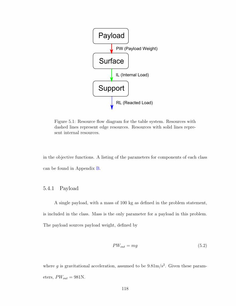
Surface
Payload
IL (Internal Load)
Support
PW (Payload Weight)
RL (Reacted Load)
Figure 5.1: Resource flow diagram for the table system. Resources withdashed lines represent edge resources. Resources with solid lines repre-sent internal resources.
in the objective functions. A listing of the parameters for components of each class
can be found in Appendix B.
5.4.1 Payload
A single payload, with a mass of 100 kg as defined in the problem statement,
is included in the class. Mass is the only parameter for a payload in this problem.
The payload sources payload weight, defined by
PWout = mg (5.2)
where g is gravitational acceleration, assumed to be 9.81m/s2. Given these param-
eters, PWout = 981N.
118

5.4.2 Surfaces
Surfaces transfer the load to the supports. They sink payload weight and
source internal load. The sourced internal load includes the sunk load as well as the
weight of the surface itself. The maximum payload weight Lmax a surface can sink
is assumed to be provided by the manufacturer. It is therefore considered to be a
component parameter. The list of all component parameters for surfaces is given in
Table 5.1. Note that not all parameters are used for determining resource flows.
Table 5.1: Component parameters for surfaces.
Parameter Description
Lmax Maximum payload weight that can be sunkm Component massl length of surfacew width of surfacet thickness of surface
Some are tracked solely for possible use in objective functions and constraints. The
resource flows of surfaces are defined by Eqs. 5.3 and 5.4.
PWin = Lmax (5.3)
ILout = PWin +mg (5.4)
A surface consumes an amount of as much payload weight as remains, up to its
maximum rated weight. It passes this weight to the supports along with its own
weight, producing an amount of internal load equal to the consumed payload weight
plus its own weight. Note how the flow of a given resource to or from a component
119

can be a function of other resource flows to or from a component. For this problem,
the resulting behavior is straightforward and trivial. However, this will lead to some
interesting implications later for more complicated problems, particularly dynamic
problems like spacecraft design.
5.4.3 Supports
The support class contains two subclasses; one containing real support cross
sections and one containing notional cross sections. For real cross sections, all
parameters are defined in the component library. For notional cross sections, some
parameters are genetically determined with an L3 genome. Both subclasses describe
supports of a constant cross section, extruded for a length of L. For this problem,
L is set to 0.75 m.
Real supports have a known cross section and material, allowing their behavior
to be determined in a simple fashion with a small number of parameters. Notional
supports, on the other hand, have their cross section defined individually using L3
genes. As a result, many mechanical properties that can be simply specified for a
real support must be calculated for each notional support in a design.
All supports sink some amount of internal load determined by their physical
properties and source some amount of reacted load, an edge resource which is trans-
mitted out of the system. The amount of internal load sunk by a support is the
maximum possible without causing Euler buckling [56]. The amount of reacted load
sourced is equal to the amount of internal load sunk plus the weight of the support
120
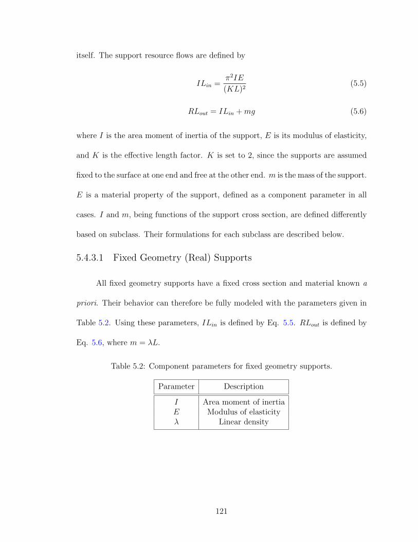
itself. The support resource flows are defined by
ILin =π2IE
(KL)2(5.5)
RLout = ILin +mg (5.6)
where I is the area moment of inertia of the support, E is its modulus of elasticity,
and K is the effective length factor. K is set to 2, since the supports are assumed
fixed to the surface at one end and free at the other end. m is the mass of the support.
E is a material property of the support, defined as a component parameter in all
cases. I and m, being functions of the support cross section, are defined differently
based on subclass. Their formulations for each subclass are described below.
5.4.3.1 Fixed Geometry (Real) Supports
All fixed geometry supports have a fixed cross section and material known a
priori. Their behavior can therefore be fully modeled with the parameters given in
Table 5.2. Using these parameters, ILin is defined by Eq. 5.5. RLout is defined by
Eq. 5.6, where m = λL.
Table 5.2: Component parameters for fixed geometry supports.
Parameter Description
I Area moment of inertiaE Modulus of elasticityλ Linear density
121
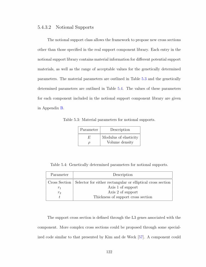
5.4.3.2 Notional Supports
The notional support class allows the framework to propose new cross sections
other than those specified in the real support component library. Each entry in the
notional support library contains material information for different potential support
materials, as well as the range of acceptable values for the genetically determined
parameters. The material parameters are outlined in Table 5.3 and the genetically
determined parameters are outlined in Table 5.4. The values of these parameters
for each component included in the notional support component library are given
in Appendix B.
Table 5.3: Material parameters for notional supports.
Parameter Description
E Modulus of elasticityρ Volume density
Table 5.4: Genetically determined parameters for notional supports.
Parameter Description
Cross Section Selector for either rectangular or elliptical cross sectionr1 Axis 1 of supportr2 Axis 2 of supportt Thickness of support cross section
The support cross section is defined through the L3 genes associated with the
component. More complex cross sections could be proposed through some special-
ized code similar to that presented by Kim and de Weck [57]. A component could
122

then be produced matching the prototype for a real support. I and λ would be
numerically determined based on the cross section developed. Due to the complex-
ity involved with generating these, they should not be modeled as having L3 genes
except under very specific circumstances. Specifically, unless the exact cross section
created can be easily reproduced with meaningful input variables which could be
optimized by the GA (something directly guiding the cross section, as opposed to a
random seed value). In such a case, this complex analysis would have to be repeated
for each crossover involving a component from this class. As may be evident, this
process would likely introduce substantial upfront computational cost to randomly
generate cross sections and determine their structural properties. This would likely
involve a separate inner optimization problem for more complex geometries.
To maintain the simplicity of this case study, the geometries possible with
notional supports were limited to simple rectangular and elliptical tubes. These
geometries are simple enough to warrant optimization within VEGA through the
use of L3 genomes. For rectangular cross sections, the outer base and height lengths
are defined by Eqs. 5.7 and 5.8, respectively:
b = 2 min(r1, r2) (5.7)
h = 2 max(r1, r2) (5.8)
The cross-sectional area is then defined as
A = bh− (b− 2t)(h− 2t) (5.9)
123

which can be simplified to
A = 2t(b+ h)− 4t2 (5.10)
and I is defined as
I =hb3
12− (h− 2t)(b− 2t)3
12(5.11)
For elliptical cross sections, the semimajor and semiminor axes are defined by
Eqs. 5.12 and 5.13, respectively:
a = max(r1, r2) (5.12)
b = min(r1, r2) (5.13)
The cross sectional area is then defined as
A = π(ab− (a− t)(b− t)) (5.14)
which can be simplified to
A = πt(a+ b− t) (5.15)
and I is defined as
I =π
4
(ab3 − (a− t)(b− t)3
)(5.16)
In either case, the support’s mechanical properties can now be defined as
functions of above properties. The linear density is defined as
λ = ρA (5.17)
and the resource flows are determined in the same way as for real supports.
124

5.5 Constraints
5.5.1 Resource Relations
For this case study, the two internal resource relations should be negative:
δPW < 0 (5.18)
δIL < 0 (5.19)
When these circumstances are met, the system has adequate capability to handle
the full payload weight, and the supports have adequate capability to handle all
load being transmitted from the surfaces. The resource relation is also negative for
reacted load, the sole edge resource in this problem:
δRL < 0 (5.20)
This implies that all load can be transmitted to the ground (out of the system).
However, the ground is assumed to sink an infinite amount of reacted load, with the
total amount of reacted load (the weight of the table plus payload) being tracked.
This is, by intention, an extremely simplistic design problem, allowing the
reader to focus their attention on the framework developed, without having any
intricacies of the specific problem to worry about (that will come later with the
spacecraft design problem). For a more complex design problem like spacecraft
design, resources may not flow directly from one class to another. Based on this
problem, it is easy to assume that all resources flow in a single line from one class to
another. In general, however, resources do not flow linearly, and do not necessarily
125
all “flow down” from “left to right” from some initial set of classes to successively
downstream sets of classes. Much of the power in the CR model arises from its ability
to decompose a system in a way where individual components can be separately
analyzed, and sources and sinks can be simply tallied and compared among all
relevant system components.
5.5.2 Component Quantity Constraints
The sole component quantity constraint in this problem is that there is a single
payload:
npayload = 1 (5.21)
This is a common situation across many design problems, certainly the spacecraft
design problem. Some “payload” component exists, and the rest of the system exists
to support that component or group of components. For a scientific spacecraft
design, for example, often a principal investigator proposing a mission has a specific
instrument or set of instruments they want to fly, and know a specific quantity
(usually one) of each that they wish to fly. In other cases, the principal investigator
may be satisfied with different combinations of instruments, as long as certain science
data return requirements are met. This will be discussed more in later chapters.
5.6 The Table Optimization Problem
We have now established the CR model for this design problem and added all
of our constraints. Our objective is to minimize the total mass of the system. A
mass has been defined for components of each class. Our objective is therefore to
126

minimize the sum of all of these defined masses, with the exception of the mass of
the payload itself:
M(C) =
system∑i=1
mi (5.22)
We can now define the CR optimization problem for this design scenario:
min M(C)
s.t. δPW ≤ 0
δIL ≤ 0
δRL ≤ 0
npayload = 1
(5.23)
5.7 Results
5.7.1 Theoretical Optimum
A single 100 kg payload is included, as dictated by the problem statement.
For all surfaces included in the surface library, Lmax is 500 N, and therefore so is
PWin. For the specified payload, PWout = 981 N, so two surfaces must be present to
fulfill the resource relation δPW ≤ 0. All surfaces considered sink the same payload
weight, so two copies of the lowest mass option must lead to the optimal solution.
They both contribute the least mass to the system, and, as a result, produce the
least amount of internal load. The lowest mass surface available, Surface1, has a
mass of 5.92 kg. With our surfaces selected, we can now determine the total amount
of internal load produced. Following Eq. 5.4, each surface produces an internal load
of 558 N. The total internal load is therefore ΣIL,source = 1116 N.
127

Determining the optimal number of supports analytically is slightly trickier.
Of the real supports considered, the RealSupoprt6, the option with the lowest λ, had
ILin = 765 N. Therefore, a single RealSupport6 is insufficient to sink the internal
load produced across the system. Two would be sufficient, however their combined
mass would be greater than a single RealSupport4, the next lowest λ real support.
For a single RealSupoprt4, with a mass of 0.56 kg, ILin = 5460 N, more than
sufficient to ensure compliance with the Eq. 5.19.
For a notional support, two factors drive the optimal support; minimization
of the support’s own mass, and maximization of its buckling load. Given Eq. 5.17,
mass of the support is minimized when the cross sectional area of the support is
minimized. ILin is maximized when I and E are maximized. E is a material
property, and is independent of cross sectional area. I, on the other hand, is a
function of the cross section. For a given cross sectional area, where the support
can buckle along the weakest axis in the plane of its cross section, the strongest
cross section is an infinitely thin circular tube [56]. For practical purposes, we limit
the minimum thickness of notional supports to 1 mm. Given this, the fact that the
cross section is circular, implying r1 = r2 = a = b = r, and assuming thin walled
tubes, Eq. 5.15 reduces to
A = 2πrt (5.24)
and Eq. 5.16 reduces to
I = πr3t (5.25)
128

Combining the objective to minimize mass with the objective to maximize strength,
we wish to maximize I/A, as a sort of strength to weight ratio:
I/A =r2
2(5.26)
It can be seen that this quantity is maximized when r is as great as possible. For
practical purposes, r was limited to be no greater than 1m, ensuring that no supports
were substantially larger than the table surface. This gives an optimal cross section
with A = 0.0063m2 and I = 0.0031m4. The optimal support, assuming a single
support is sufficient in some case, is the one with the lowest mass (which will be
implied for a fixed cross section by lowest ρ) which can sink an internal load of 1116
N. The lowest density support material considered is 6061 aluminum, with a support
mass of 12.7 kg at the specified dimensions. For 6061 aluminum, E = 6.9(1010)Pa.
This leads to the specified support having a capability to sink 9.5(108)N, far beyond
the internal load produced in the system. Due to the finite minimum thickness of
the support, it is possible to decrease the radius of the support, decreasing I/A, but
simultaneously decreasing the cross sectional area. Rearranging Eq. 5.5 to solve for
I,
I =ILin(KL)2
π2E(5.27)
which, for 6061 aluminum, leads to a required I = 3.69(10−9)m4. Using Eq. 5.25,
this results in r = 1.1cm, which in turn leads to an area of 6.6(10−5)cm2, and a mass
of 0.13kg. This is less than the mass of a single RealSupport4, and is therefore the
minimum mass support.
129

This solution produces the bill of materials outlined in Table 5.5, leading to a
theoretical minimum mass of 11.97 kg.
Table 5.5: Bill of materials for the theoretical minimum mass table.
Component Quantity Mass (kg)
Payload 1 0Surface1 2 5.92
6061 AL support 1 0.13
Total - 11.97
5.7.2 CR Framework Optimal Result
The table optimization problem was set up using the CR model and frame-
work, and optimized with the parameters listed in Table 5.6. Any parameters not
listed have their default values discussed above. Over ten trials, the CR framework
Table 5.6: Tuning parameters used for the table problem in VEGA.
Parameter Value
Population Size 500Elite Fraction 30%Mutation Rate 1%
converged in eight cases to an optimal design with a mass of 12.4 kg, coming within
4% of the theoretical optimum. In the remaining two cases an optimal design with
a mass of 12.9 kg was achieved, within 8% of the theoretical optimum. The conver-
gence of the fitness values are given in Fig. 5.2. For each design, the fitness score
is expressed in this figure as -1 times the combined mass of the payload and table.
The difference between the 12.4 kg tables and the theoretical optimum was in the
130

5 10 15 20 25 30
−126
−124
−122
−120
−118
−116
−114
−112
Generation
Fitn
ess
scor
e (−
kg)
Figure 5.2: Fitness evolution for the table design problem. Ten trials areshown. A solid line represents the fitness score of the most fit individ-ual in each generation, and a dashed line represents the average fitnessof the whole generation, with solid and dashed lines of the same colorcorresponding to the same trial.
supports used. While the theoretical optimum utilized an optimal notional support,
as discussed above, the genetically determined optimum in each case utilized Real-
Support4, the optimal real support. The design achieved in the 12.4 kg cases is in
fact the optimal design, should the notional support subclass be removed from the
problem.
The framework therefore seems to show a behavior of favoring “real” compo-
nents over notional ones when both serve the same role. This is likely due to the
131

fact that the available real components have already been independently optimized.
Conversely, the notional components start with random internal design parameters,
and must be optimized by VEGA over the course of the overarching design opti-
mization. However, in the presence of better performing real components, VEGA
will quickly eliminate the yet-to-be-optimized real components.
This demonstrates a need for some important considerations. VEGA is de-
signed to address a component selection problem. It is not intended to perform
“local” optimization within a single component or subsystem. It may be possible to
pair it with an additional, dedicated component optimization step, but this must be
weighed against the increased computational cost. When a real and notional class
exist that serve the same purpose, the design optimizer will often favor real compo-
nents. Usually this occurs when a very specific combination of L3 genes is required
for component optimality. Therefore, the number of variables in any component’s
L3 genome should be limited to the minimum, and the components “pre-optimized”
with reasonable simplifying assumptions. In this table design problem, for exam-
ple, the assumption could be made that thin walled tubes are used, perhaps setting
t = max[r1,r2]10
. Further, it has been analytically shown that optimal supports will be
those with r1 = r2, since buckling will occur along the lowest I axis. These consid-
erations reduce the number of L3 genes from four to two, increasing the probability
that random combinations of genes will lead to more optimal supports than the real
supports.
Additionally, increasing the mutation rate of L3 genes could favor more rapid
identification of viable notional components, although this comes at a cost in other
132

performance areas. What is better is to consider the notional components essentially
fixed when they are created. It should not be assumed that VEGA will optimize in-
dividual notional components. Their genetic parameters should be carefully chosen
to encourage viability with this consideration in mind.
Conversely, this behavior of favoring “off the shelf” components may actually
be desirable, particularly in the realm of spacecraft design. There is often a lower
cost, financially and in other ways, in using off the shelf components.
This behavior illustrates an important aspect of automated design optimiza-
tion. Such tools are useful for trade space exploration in general, allowing one to
compare a number of design options. However, they do not necessarily produce
a truly optimal design or make all necessary considerations for a design proposal.
For the foreseeable future, it will be necessary to perform human-based tuning and
refinement of the design options chosen from the trade space.
133
Chapter 6: The General Dynamic CR Model
6.1 Overview
This chapter extends the CR model developed thus far to handle systems whose
behavior varies with time. This is important, since the vast majority of spacecraft
design problems do have a changing behavior with time. In orbit of any planetary
body, the resource flows of the spacecraft will change over the course of an orbit.
Even for missions which do not orbit a planetary body, there will generally be a
number of mission phases, each with their own spacecraft behavior.
In the dynamic model, we must account for a system which must respond to an
external environment which changes over time. This will be accomplished by eval-
uating the state of the system at a number of discreet timesteps. The environment
will be expanded in scope, with edge flows, as well as other environmental properties,
taking on given values for each timestep. Then, within each timestep, the system
can be viewed as static (or at least quasi-static), and can be evaluated following the
logic already outlined, with a few additional considerations which will be detailed
in this chapter. After the simulation (iteration of evaluation through all timesteps)
is complete, we can assess penalties and determine objective values for a given de-
134

sign, for use in optimization. Penalty values are determined for each timestep, with
penalties across all timesteps summed to determine the entire penalty.
There are a few key differences from the static CR model. For the dynamic
model, the environment has been developed into its own component-like object.
The environment is modeled as a sort of quasi-component, with its own sources and
sinks, whose properties are allowed to change over time. A more involved simulation
of the system over the period of evaluation/interest (henceforth referred to as the
simulation window) is now required. Within this simulation, each timestep has a set
duration. Each timestep is evaluated essentially using the static CR model. Rather
than having a fixed amount of flow for each relevant resource, each component
now has a flow rate for each relevant resource. As a result, all net flows, which
were total flows in the static CR model, are now flow rates, assumed constant
over the duration of each individual timestep. Therefore, the total net flow over a
given timestep is determined by multiplying the net flow rate by the duration of
the timestep. Additionally, the environment is now referenced by all components,
containing properties in addition to edge flows that can change over time. All actual
system components (not including the environment) must then obey the following
rules:
1. A component’s external behavior is entirely captured by the resources flowing
to and from it.
135

2. If a component is not a store, its behavior within a given timestep is dependent
solely on the environment. It does not depend on any internal net flows or on
the state of any other components.
3. If a component is a store, its state may additionally be a function of the
net flow of that resource, with the order of flow with stores determined by a
priority for each reservoir. Otherwise it must follow the above rules.
The simulation proceeds following the general algorithm outlined below:
while !simComplete
step environment forward
timestep++
if timestep > final timestep
simComplete = true;
else
simulation time += duration(timestep)
update all edge nodes
if simulation time > maximum simulation time
simComplete = true;
else
simComplete = false;
end
end
end
if !simComplete
update resource flows for sources and sinks
tabulate net flows
update resource flows for stores
calculate resource relations for this timestep
end
end
apply constraints to design
determine fitness of design
There may be additional steps, particularly within the operation of the environ-
ment, depending on the problem at hand. Later chapters, will outline the specific
136

environment used for spacecraft design for this work. A complete source code for the
framework, including this simulation, will be published upon completion of scouring
of proprietary and privileged data.
6.2 The Environment Object
The behavior of the environment is largely dependent on the design problem
at hand. Just as the resource flows of a component are driven by the internal
models specific to that component class, the edge flows of the environment are
driven by time-varying models of the environment specific to the design problem.
These models set fixed values for each resource flow at each timestep. The system
can therefore be analyzed at a single snapshot in time to determine its feasibility
and performance. Analysis that is essentially identical to that of the static CR
model is performed at each timestep. The biggest differences are that all component
behaviors may be a function of a number of environment parameters, and that the
state of reservoirs carries over from one timestep to the next. After the simulation
is complete, the penalty values from each timestep are summed, providing a total
penalty value for any infeasible design. Objective functions are then evaluated
following the same scheme as in the static CR model.
The biggest difference between the static and dynamic CR models is the treat-
ment of the environment external to the system. In the static CR model, the en-
vironment was treated simply as a set of steady state edge nodes. In the more
general dynamic CR model, the system may not be in steady state throughout the
137

simulation window. Thus, in the static CR model, the environment contains its own
models and additional properties which may act as inputs to the component level
simulations. In general, an environment object must include three sets of informa-
tion at any given timestep; nodes for all edge flows, at the current timestep i, and
the duration of the current timestep ∆ti.
Just as the component classes will be different for each design problem, so too
is the structure of the environment different for each design problem. The level of
complexity is similarly variable, as chosen by the user. Consider an extension of
the lighting system design problem from Chap. 3. Let us say that this is a solar
powered lighting system, designed to collect and store energy while illuminated, and
then supply power to the lamp when the system is unlit. The CR diagram for the
system, originally presented as Fig. 3.2, is shown here in Fig. 6.1, modified for
treatment as a dynamic system. As before, boxes in the diagram within the system
represent components, and the “environment” box outside the system represents
the environment object.
Lines connecting components to the environment are not the only information
about the environment available to a given component. For example, within a given
timestep, the lamp’s mode is determined by the state of the sunlight resource, even
though sunlight does not flow directly to the lamp. One may intuitively draw the
conclusion that the power source could supply power to the lamp when unlit, and
based on this electrical power flow the lamp could turn on. This is the straight-
forward description of what is physically happening in the system. However, this
would require that the lamp’s behavior be dependent on the state of other compo-
138

Environment
Lamp
Electrical Power
LightHeat
System
Environment
Sunlight
Figure 6.1: Revised, dynamic lighting system example. The environmentis now a standalone object, with three edge flows with the system.
nents within the system, indirectly, through resource flows. For reasons that will be
discussed in section 6.3, the rules listed in section 6.1 must be imposed. As a result
(and to preserve generality), the state of the lamp cannot depend on the power
generation state of the power source. Instead, the lamp will be in an “off” state
whenever the flowrate of sunlight from the environment is above some critical level,
and will in an “on” state at all other times.
6.3 Dynamic Resource Flows
In dynamic CR problems, having a component’s behavior be a function of
it’s resource flows leads to two coupled issues; it can lead to transcendental loops,
and the flow state of the system becomes ambiguous, potentially dependent on the
139

Solar Array
BatteryAll other
components
Radiator
Environment
System
Solar Flux Radiated heat
HeatElectrical
Power
Figure 6.2: An extremely simplistic spacecraft system. All componentsother than solar arrays, radiators, and batteries are lumped together.They are assumed to simply consume electrical power and produce heat.
order in which components are updated. Consider, as an example, a most sim-
plistic spacecraft design, shown in Fig. 6.2. Solar arrays produce electrical power
and heat, both linearly proportional to the flow of solar flux from the environment.
Radiators consume heat produced within the system and radiate it to the environ-
ment. They are assumed to require an amount of electrical power proportional to
the heat rejected to operate. Batteries are a store, consuming any excess electrical
power surplus to fill their electrical power reservoirs, and supplying electrical power
from their reservoirs to close any deficit. In either mode, batteries produce heat
proportional to their electrical power flow rate. All other components are lumped
together, and assumed to consume electrical power and produce heat. Other aspects
of their behavior are not relevant to this example. At this point, a few of issues
140
may be apparent. The order in which components update now matters. The mode
in which batteries operate, and the flow rate of heat from them, is a function of the
net electrical power flow. The amount of electrical power consumed by the radiator
is dependent on the heat it is rejecting. The state of each battery and radiator is
dependent of the net resource flows through the system. The relevant net flows for
each component cannot be known until the other is fully simulated. Thus a sort of
”transcendental loop” forms, where the state of multiple components are dependent
on each other. None can be simulated until they are all simulated.
A few potential solutions exist to solve this problem. Timesteps can be held
to sufficiently short duration that each component’s state can be solved using the
net flows from the previous timestep, without a significant accumulation of error.
Alternatively, the states of any components in transcendental loops can be iteratively
solved, continuing to update the state of all components in the loop until each of their
states is stable. Both of these options were avoided, as, depending on the particular
design problem, they have the potential to become very computationally intensive.
In the dynamic CR model, the problem is solved by imposing rules two and three
listed in section 6.1. Applying rule #2 to radiators, radiators will be assumed to
operate at a set power level, consuming heat from the system at a given time. The
net flow of heat can then be constrained to be less than 0 within the system. That
is, those components which consume heat must always have the capacity to consume
at least as much heat as is being produced for the system to be considered feasible.
The state of radiators are now only dependent on the environment (through their
141

internal models, which account for the background temperature of the environment
to which they are radiating).
Applying rule #3 to stores, we see that their state is still dependent on internal
net flows. Therefore, their behavior (at least the portion involving their reservoirs)
must be determined after the state of the rest of the system is determined. Once
the rest of the system has been simulated, we can determine if we have an electrical
power surplus or deficit, and update the state of the batteries accordingly. There
is still the possibility that the state of some store may rely on the state of another
store. When a reservoir updates, it may change the state of its component, altering
additional net flows within the system. Since all non-reservoir components in the
system adhere to rule #2, this only affects other stores. Therefore, a priority must
be assigned to each reservoir, used to determine the order in which they update.
Priority may need to be carefully chosen by the user to ensure realistic simulation.
Ultimately, an end user should be able to use a design tool powered by this
framework without intimate understanding of the framework itself. As will be de-
tailed below, reasonable options for spacecraft design are chosen for many properties
of the dynamic CR framework. Other values for these properties may be better
suited for other design problems. It is also of note that adherence to the rules
discussed here does mean that the dynamic CR model may be conservative, not ac-
curately predicting the optimal behavior of the system throughout the simulation.
The dynamic CR model can confirm feasibility of a given design, but as a result of
conservatism, under the right circumstances a design found to be infeasible by the
dynamic CR model may in fact be feasible.
142
6.4 Stores in dynamic simulations
In the quasi-static CR model, net flows were still of a constant amount of
each resource. If, before considering stores, any resource relations were violated, it
was sufficient simply to check if stores had the capacity to, based on their initial
state, consume any undesired surplus or supplement a flow to close any undesired
deficit for a given resource. In the dynamic CR model, resource flows are really flow
rates. Additionally, stores contain some internal reservoir, which can be drained
and replenished over time. We must do two things when evaluating resource flows
with stores. first, we must take the net flow rate, and factor in the duration of the
timestep to determine the total resource deficit and surplus. Second, if the state of
a store’s reservoir has been updated by a deficit or surplus, that state must persist
from one timestep to the next.
Consider the second consideration first. For each resource j for which a com-
ponent is a store, it contains a reservoir with, at any point in time, a current fill level
fcj. The fill level is bounded by a maximum fill level fmax,j and minimum fill level
fmin,j. All stores are initialized as either full fcj = fmax,j or empty fcj = fmin,j. The
fill level of the reservoir can then vary between fmin,j and fmax,j over the duration
of the simulation.
The general logic for stores within a given timestep is as follows. It is assumed,
as described in section 6.1, that initial net flows δj0 have already been tabulated
based on all sources and sinks in the system. For each δj0 there is an associated
143
resource relation of the form of either Eq. 4.6 or 4.7. With stores, the desire is to
drive this net flow rate towards the “ideal” value, Kj, i.e.,
δj = Kj (6.1)
The remaining question is, if multiple stores exist for a given resource, in what
order should they be updated? It is possible to have multiple component classes
in a design which contain a reservoir for the same resource. The rate at which
resources flow to or from a reservoir could affect the overall state, and therefore
other flows of the component. Without knowing specific details of the component
classes involved, it cannot be known what these ripple effects may be. To solve this
issue, each component class containing a store was assigned a priority. Within a
given class, priority order is determined by the order in which components appear
in the chromosome for that component class. Stores are then evaluated in order of
descending priority (from highest priority to lowest priority).
Within a given timestep, flow into or out of any store is as follows. For a given
resource i, define the resource flow gap γj as
γj = δj0 −Kj (6.2)
such that γj > 0 implies a surplus, and γj < 0 implies a deficit. γj should be driven
towards 0 through the use of stores. For a given store for resource j, the total
resource gap over the timestep j, Γj = γj∆ti, is calculated. The fill is then updated
based on Γj:
144
fcj = fcj + Γj (6.3)
If, after doing this, fcj is beyond the bounds fmin,j and fmax,j, it is set to the closer
bound, and Γj is set to the remainder between fcj and that bound. If fcj is within
bounds, Γj is set to 0. As long as Γj is nonzero, the framework continues moving
through the list of available stores. Finally, the remaining net flow after considering
all stores is averaged over the duration of the timestep. That is, after achieving
Γj = 0 or exhausting all available stores, γj is set to Γj/∆t. From the change in fcj
over ∆t, a flow rate into the store can be determined. It is then possible for this flow
with the store to modify the state of the component. For example, considering a
battery as a store, charging or discharging a battery will generate heat proportional
to the power level at which the battery is charging or discharging.
6.5 Module Components
In certain complex cases, including satellite design, it becomes necessary to
consider interoperation between what would otherwise be considered separate com-
ponents. For example, consider a spacecraft transmitter and antenna. Physically,
they are separate components. Within the CR model, an antenna would sink a sig-
nal, radiating it as a telemetry stream to the environment. The transmitter would
sink data, and source a signal (modulating the data onto a signal to be transmitted).
However, the properties of the signal radiated by the antenna will be a function of
the input signal from the transmitter, depending on the power level and frequency
145

of the signal to determine the radiated power and gain of the antenna. Thus their
behavior cannot be independently modeled. The state of the antenna depends on
the properties of the internal signal flow. This violates rule #2 of the dynamic CR
model.
The solution adopted is the introduction of a new concept to the CR model: the
module component. Modules function externally as a single component. A module
as a whole must follow the same rules as any other component class. Internally,
they appear as their own quasi-systems. They behave in a similar manner to a CR-
modeled system. They are similarly organized, constructed out of subcomponents
of varying classes. When present in CR optimization problems, modules feature
an L3 genome which resembles a CR system’s L2 genome, defining their internal
subcomponents. It contains a chromosome for each subclass of the module, and
contains all subcomponents as child objects. The module initializes in a similar
way to a proper system, populating components class by class based on its genome.
Specific module classes may define additional properties. For modules in general,
the only additional property is mass, which, unless otherwise noted, is assumed to
be the sum of the mass of its subcomponents. For an example of a module and its
subclasses, see section 7.4.3 for a full discussion of an RF subsystem modeled as a
module.
146
6.6 Summary
This chapter has extended the static CR model to handle the design of systems
whose behavior changes over time, creating a dynamic CR model and simulation
framework. In the static CR model, the environment was merely a set of sources
and sinks (nodes) for edge resources. In the dynamic CR model, the environment
has been extended into a component-like object which not only contains edge nodes,
which now may change over time, but also contains additional properties specific to
the problem at hand. Resource flows have changed from fixed quantities of resources
produced and consumed by components to flow rates, over a variable timestep, with
time dictated by the environment object. In the static CR model, system objectives
and constraints could be evaluated merely considering fixed properties of the system
components, and by balancing the resource flows at a fixed point in time. In the
dynamic CR model, this resource balance still occurs, and components still have
the same sort of additional properties for objective function evaluation. However,
the resource balance must now be performed at each timestep of the simulation,
with considerations made to avoid ambiguous flow behavior, such as resource flow
loops. With this more complex treatment of resource flows, we have extended stores
from their rudimentary existence in quasi-static CR problems. Stores now track
their internal state from one timestep to the next, and use a somewhat modified
component update logic from the quasi-static case.
Unfortunately, with this added complexity, a significant amount of problem
specific work must be performed to craft an environment for each design problem.
147

The following chapter presents a general form of an environment object which may
be applied to a wide range of spacecraft design problems. While specialized portions
of the model are now required which specific to the design problem, A dynamic
model that is still general enough to, without modification, address a wide range of
spacecraft design problems may be developed.
148
Chapter 7: The Dynamic CR Spacecraft Design Framework
7.1 Overview
The discussion of the CR model thus far is generally applicable to any system
that can be modeled as a collection of components and resources flowing between
them. However, the goal of this dissertation is to develop a framework for to facilitate
satellite design and trade space exploration. Chap. 2 discussed one case study, LEO
ADR. An additional, somewhat simpler problem is the design of an Earth observing
cubesat on a fixed orbit. Addressing these design problems through application of
the CR model will serve as a proof of concept and validation of the model.
This chapter discusses the specifics of spacecraft design using the dynamic
CR model. The discussion will remain as general as possible. The specifics of the
General Evolutionary Spacecraft Design Analyzer (GESDA) described here, powered
by VEGA and the CR model, are therefore applicable to a wide range of spacecraft
design problems. For this dissertation, the scope was limited to Earth orbiting
satellites, and separated into two cases. The first models a ”simple passive” satellite
that is assumed to be on a fixed orbit. In this context, ”passive” means that the
spacecraft does not interact with its environment (except in the context of edge
flows and reading the state of environment properties). This includes those mission
149

types within the range of applicability of the GINA model, such as communications
satellites, Earth observation satellites, and scientific missions in a fixed orbit.
The second model is an extension of the first, capable of modeling an “active”
satellite, where the satellite is expected to maneuver and/or interact with its envi-
ronment. Even if the spacecraft is “active” (e.g. with a radiating antenna or laser
altimeter) these spacecraft do not change the state of the environment, or their own
structure over the simulation window. By contrast, active satellites either maneuver
or physically interact with their environment. Examples of such missions include
ADR missions, interplanetary sample return and surface missions, robotic satellite
servicing.
Specific examples of applications of the simple and complex satellite models
will be presented in Chap. 8 and 9, respectively. Chap. 8 will validate the simple
satellite model, comparing a design for an Earth imaging cubesat to a Dove cube-
sat developed by Planet Labs [58]. Ultimately, Chap. 9 will validate the GESDA
and the complex satellite model by revisiting the LEO ADR study of Chap. 2, this
time performing the vehicle design using GESDA. In both cases the results ob-
tained with GESDA are validated through comparison to previous data from the
missions/studies they are replicating.
7.2 Resource Flow for Spacecraft Design
The general CR model for spacecraft design is as shown Fig. 7.1.
150

Pow
er
Genera
tion
Pow
er
Sto
rage
Thru
ste
r
C&
DH
/Data
Sto
rage
Paylo
ad
Pro
pellant
Tank
RF M
odule
electrical power
pro
pellant
Spacecraft
Envrionment
thru
st
data
telemetry
sola
r flux
Fig
ure
7.1:
The
CR
flow
dia
gram
for
gener
aliz
edsp
acec
raft
des
ign.
151

The topology shown is for an active spacecraft. The topology is essentially the
same for a passive spacecraft, with the exception that the thruster and propellant
tank classes may not be present. They may be required for a passive spacecraft if
attitude control requirements are under consideration (they were not in the scope of
this work), in which case they could be re-added to the CR model. Three internal
resources, data, electrical power, and propellant, and three edge resources, solar
flux, telemetry, and thrust, are present in this problem. Their resource relations are
as given below, respectively:
δdata < 0 (7.1)
δpower > 0 (7.2)
δprop > 0 (7.3)
δsolflux ≥ 0 (7.4)
δtlm < 0 (7.5)
δthrust < 0 (7.6)
The payload produces some amount of data throughout the simulation, and Eq. 7.1
results from the constraint that the spacecraft must be able to handle all data
produced by the payload. Eq. 7.2 results from the constraint that the spacecraft
must be able to supply at least as much power as it is consuming at any given point.
Eq. 7.3 results similarly that the spacecraft must be able to supply propellant at a
152
rate sufficient to feed any active thrusters. Data flow is measured in bits per second,
power flow is measured in W, and propellant flow is measured in kg/s.
The issue of interoperability arises with the flow of power and propellant
throughout the system. A power source will supply power within a certain volt-
age range, and all power sinks will require power within a certain voltage range.
Thrusters are designed to use a given mix of propellants, and any tanks onboard
must supply the proper propellant to a given thruster. For electrical power, a survey
of spacecraft components, conducted to populate the GESDA component libraries,
revealed that voltages of spacecraft components are largely standardized to a small
number of voltage ranges. Additionally, the voltage of power sources considered can
be easily reconfigured through the wiring of battery and photovoltaic cells, changing
the voltage and current output of the component without changing the power out-
put. Therefore, it was assumed that the voltage ranges of individual components is
beyond the scope of necessary considerations at this high level of spacecraft design,
so interoperability of electrical power was not considered.
On the other hand, it is not uncommon for spacecraft to have multiple propel-
lants onboard to support dissimilar thrusters with different propellant requirements.
Therefore, the propellants shown in Table 7.1 were considered, each modeled as a
separate resource. Table 7.1 also lists the density of all liquid propellants considered,
and the molar mass of all gaseous propellants considered. Additional interoperability
considerations beyond resource flows are required for certain components. These are
covered by the inclusion of module components, which are discussed in section 7.4.
153
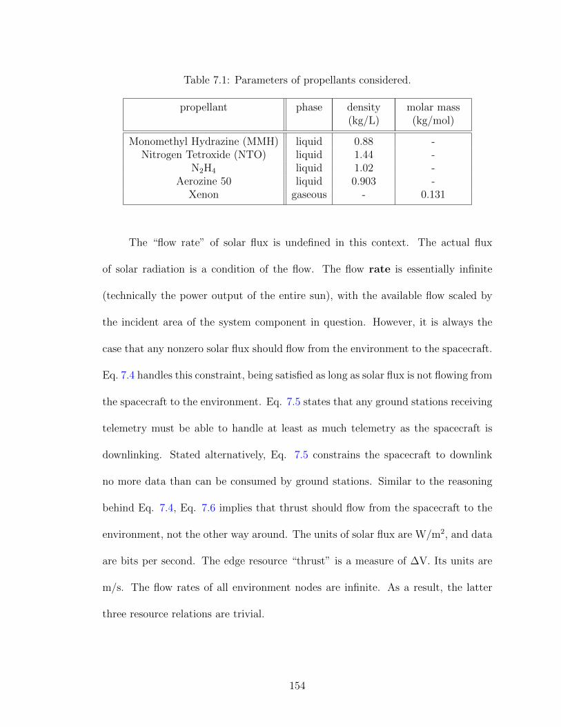
Table 7.1: Parameters of propellants considered.
propellant phase density(kg/L)
molar mass(kg/mol)
Monomethyl Hydrazine (MMH) liquid 0.88 -Nitrogen Tetroxide (NTO) liquid 1.44 -
N2H4 liquid 1.02 -Aerozine 50 liquid 0.903 -
Xenon gaseous - 0.131
The “flow rate” of solar flux is undefined in this context. The actual flux
of solar radiation is a condition of the flow. The flow rate is essentially infinite
(technically the power output of the entire sun), with the available flow scaled by
the incident area of the system component in question. However, it is always the
case that any nonzero solar flux should flow from the environment to the spacecraft.
Eq. 7.4 handles this constraint, being satisfied as long as solar flux is not flowing from
the spacecraft to the environment. Eq. 7.5 states that any ground stations receiving
telemetry must be able to handle at least as much telemetry as the spacecraft is
downlinking. Stated alternatively, Eq. 7.5 constrains the spacecraft to downlink
no more data than can be consumed by ground stations. Similar to the reasoning
behind Eq. 7.4, Eq. 7.6 implies that thrust should flow from the spacecraft to the
environment, not the other way around. The units of solar flux are W/m2, and data
are bits per second. The edge resource “thrust” is a measure of ∆V. Its units are
m/s. The flow rates of all environment nodes are infinite. As a result, the latter
three resource relations are trivial.
154

The model topology presented here should be considered a general template
for a spacecraft design, which can be used for a wide range of missions. However,
the capability of the framework is not limited to this specific topology. Neither
satellite design problem studied in this work uses all component classes defined in
Fig. 7.1. Additional satellite design problems may require additional component
classes and resources. These can be easily added for the problem at hand. To
do so, the user must only specify the internal model for new component classes
for determining their resource flows, and a resource relation for any new resources.
For example, consider a trade study investigating how the use of a thermodynamic
power generation subsystem (such as a space-based nuclear reactor, or sterling engine
based solar concentrator), compared to conventional space-based power generation,
such as photovolatic arrays (conventional solar panels). The design of the thermal
management subsystem has a significant effect in overall system performance in the
design space. One would introduce heat as an additional resource. For thermal
stability, the spacecraft must be balanced such that it can always reject at least as
much heat as it is producing. Therefore, the resource relation for heat would be
δheat < 0 (7.7)
In addition to being electrical power sources, these new power generation subsystems
would also be heat sources. A new component class is then required that can act
as a heat sink. One could introduce a “radiator” class, which would sink heat
and electrical power at given rates. The electrical power sink rate would likely be
155

constant. Depending on the fidelity of the radiator class’s internal model and of the
environment, the heat sink rate may also be constant, or may be a function of the
environment at the current timestep.
As can be seen in this example, no modification of the overall framework is
required to introduce a whole new class of components. Resource flows are pooled
between all components. This adds a layer of abstraction between all component
classes, so the existing topology is essentially agnostic to the addition or removal of
component classes. The only new information that is required is the internal model
for the new component class and the resulting resource nodes.
7.3 The GESDA Environment
Typically, the environment must be purpose-built for the design problem at
hand using the dynamic CR model. A generalized environment object was devel-
oped which could be used for any spacecraft design problem. For reasons that will
be discussed in greater depth below, the nature of the environment is more com-
plex for spacecraft which maneuver. This is because the simulation contained in
the environment is of variable time, depending on how long it takes the spacecraft
to complete each maneuver. For passive spacecraft, a much simplified environment
can be used, which handles a simulation over a fixed time period, such as an inte-
ger number of orbits. The remainder of this section is therefore divided into two
subsections, each covering a different spacecraft environment. The first is a passive
environment, which has a much smaller, fixed size simulation window, but simulates
156

the environment at a higher fidelity. The second, based upon the first, simulates
an active environment. It has additional functionality to handle a variable simula-
tion window and maneuvers, but is lower fidelity to keep runtimes manageable for
GA-based optimization. It is hoped that future computational advancements, along
with a re-write of the simulation in a faster language than Matlab, will facilitate
high fidelity active simulations. Section 7.3.1 lays the groundwork for the satellite
environment in general, describing it up to the point necessary to simulate a passive
spacecraft. Section 7.3.2 then discusses the changes and extensions necessary to the
passive environment to simulate active spacecraft.
7.3.1 The Passive Satellite Environment
In general, the environment object is built around a simulated orbit or trajec-
tory. External simulation or analysis is used to, determine the values of the param-
eters that drive environmental behavior at each timestep. For the work presented in
this dissertation, external simulation was performed in the General Mission Analysis
Tool (GMAT) to determine simulation step sizes, and available solar flux at each
timestep. AGI’s Systems Toolkit (STK) was used for communications access calcu-
lations. An additional, user defined dataset determines the observation windows in
which the payload is active. In the case of multiple payloads, this dataset takes the
form of a table with a column for each payload. The timestep and solar flux data
from GMAT are concatenated with this payload scheduling data to create an input
data file for environment creation. Table 7.2 gives the format of this simulation
157

data. The first column gives ti, the elapsed time at which the timestep begins in
Table 7.2: Simulation data format.
ti (s) φsol payload1 payload2 ...
51.65 1.03 1 0 ...
seconds. The second column gives φsol, the solar flux, normalized by the solar flux
at Earth, which is assumed to be 1367 W/m2. The remaining columns are binary,
with 1 indicating a given payload is active, and 0 indicating it is not. A separate
file contains the access information from STK. This file lists communications passes
with user-selected ground stations.
At a given timestep i, the duration of the timestep ∆ti is determined as
∆ti = ti − ti−1 (7.8)
therefore, the duration of the 0th timestep is undefined. Φsol,i, the actual solar flux
at ti is defined as
Φsol = ΦEarthφsol = 1367 W/m2φsol (7.9)
For downlink access, a list of terminals is supplied, along with the compatible
downlink bands, and G/T of each station in each band. An example communications
pass is given in Table 7.3: Terminals can either be ground terminals, such as SG1
at Svalbard [59], shown in Table 7.3, or space terminals, that is, relay spacecraft,
such as one of NASA’s Tracking and Data Relay Satellites (TDRSS). If a given
timestep falls within a communications pass, the environment’s link parameters will
158

Table 7.3: Example communications pass.
Ground Terminal - SG1
ti (s) range (km) elevation (deg)
897.855 2548.776 -21.746957 2154.629 -22.095
1017.000 1769.16 23.361077.000 1412.368 26.0351137.000 1114.424 30.5261197.000 935.2109 35.2711257.000 945.6845 34.9661317.000 1140.528 30.0891377.000 1446.413 25.7931437.000 1806.806 23.291497.000 2193.794 22.1321552.685 2565.077 21.843
be interpreted by linearly interpolating the range and elevation of the spacecraft.
Unless otherwise noted, the following parameters are used for link calculation across
all designs and possible orbits: the 6 dB Eb/No assumes Reed-Solomon(255,223)
Table 7.4: Link parameters assumed across all designs and orbits.
Bit Error Rate (BER) 10−5
Eb/No 6 dB
encoding. For the purposes this work, this value was hard coded into the design
problems addressed. Future extensions of this work could consider the encoding
used as a design parameter, with multiple possible encoding schemes selected from
using an L1 gene. If multiple orbits are under consideration, a separate input data
file is created for each of them. If optimization is being performed, an L1 gene is
159

used to specify the orbit chosen for a given design, such that the selection amongst
orbits under consideration can factor into the global optimization.
Since passive spacecraft do not maneuver, this covers the only two edge re-
sources, solar flux and telemetry, as well as the additional environmental parameters
for which payloads are currently operating. The flow rate of solar flux is infinite.
The environment is assumed to provide an infinite flow of solar radiation over an
infinite area, with the actual amount captured by a component determined by that
component’s area. The actual flux Φsol in W/m2 is captured in the conditioning of
the environment’s solar flux source. Similarly, the flow rate of telemetry is negatively
infinite. That is, the environment has an infinite capacity to sink telemetry from the
spacecraft. However, similarly, the conditioning of the environment’s telemetry sink
provides the limiting factor on the actual rate at which telemetry is “dissipated”
from the spacecraft. This is accomplished through link budged analysis, as will be
discussed in section 7.4, using the range and G/T of the ground station being used
and the transmitter properties of the RF module onboard the spacecraft. Binary
properties exist within the environment object which update at each timestep with
edge nodes, dictating whether or not each payload is active. In the next subsection,
we will extend and modify this environment object to handle active spacecraft, with
particular attention paid to LEO ADR spacecraft.
160

7.3.2 The Active Satellite Environment
The active satellite environment is fairly similar to the passive environment
with two key differences; complex interactions with the environment, and a proce-
durally generated simulation. In terms of edge resource flows, the active satellite
environment is similar to the passive satellite environment. The only change is the
addition of a ∆V store. The simulation is procedurally generated, as discussed be-
low, based on the completion of scheduled maneuvers. This ∆V store contains the
remaining ∆V that must be completed for a given maneuver. Once the store is “de-
pleted”, the simulation can move on to the next maneuver at the next procedural
update.
More complex interactions between the spacecraft and the environment are
required than for a passive satellite, largely tied to performing maneuvers. For
example, an ADR spacecraft must rendezvous with, capture, and potentially repo-
sition a debris object. These complex interactions have complex (and coupled)
implications on the behavior of the spacecraft. A spacecraft’s mission, generally
speaking, can be considered to start from an initial orbit, and maneuver in such a
way to arrive at a number of waypoints, potentially with different operating modes
driven by the payload and mission at and around each waypoint. The logistics of
travel between these waypoints is dependent on the capabilities of the spacecraft,
which will vary based on the configuration of onboard components. Especially when
this framework is being used for optimization, multiple spacecraft may be under
evaluation with no a priori knowledge of spacecraft configuration. In particular,
161
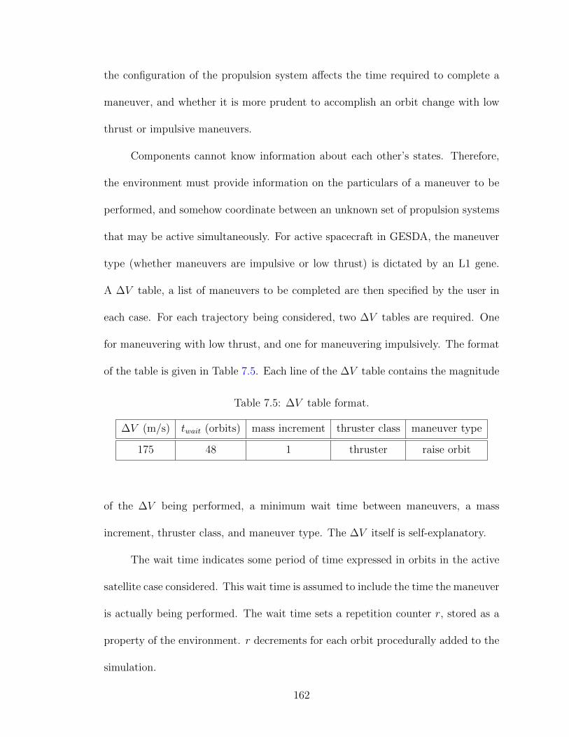
the configuration of the propulsion system affects the time required to complete a
maneuver, and whether it is more prudent to accomplish an orbit change with low
thrust or impulsive maneuvers.
Components cannot know information about each other’s states. Therefore,
the environment must provide information on the particulars of a maneuver to be
performed, and somehow coordinate between an unknown set of propulsion systems
that may be active simultaneously. For active spacecraft in GESDA, the maneuver
type (whether maneuvers are impulsive or low thrust) is dictated by an L1 gene.
A ∆V table, a list of maneuvers to be completed are then specified by the user in
each case. For each trajectory being considered, two ∆V tables are required. One
for maneuvering with low thrust, and one for maneuvering impulsively. The format
of the table is given in Table 7.5. Each line of the ∆V table contains the magnitude
Table 7.5: ∆V table format.
∆V (m/s) twait (orbits) mass increment thruster class maneuver type
175 48 1 thruster raise orbit
of the ∆V being performed, a minimum wait time between maneuvers, a mass
increment, thruster class, and maneuver type. The ∆V itself is self-explanatory.
The wait time indicates some period of time expressed in orbits in the active
satellite case considered. This wait time is assumed to include the time the maneuver
is actually being performed. The wait time sets a repetition counter r, stored as a
property of the environment. r decrements for each orbit procedurally added to the
simulation.
162

The mass increment indicates that some mass should be added or subtracted
from the spacecraft at the end of the maneuver. For orbital debris removal, for
example, this could be the addition of a debris mass after completing rendezvous,
or, in the event of a negative increment the jettisoning of a debris object, spent
stage, or some other mass from the spacecraft. The units and amount of mass
that comprises a mass increment is specific to the design problem, so a property
exists within the payload component class to set it. For example, if a spacecraft
is grappling a 1000 kg mass at the end of a maneuver, a mass increment of 1 in
the ∆V table means that the spacecraft’s mass would be increased by 1000 kg in
the simulation. A mass increment of -1 means that the spacecraft’s mass would be
decreased by 1000 kg in the simulation.
The thruster class indicates what component class performs the maneuver.
For example, a mission may perform large maneuvers with a low thrust electric
propulsion system, while performing proximity operations or terminal guidance with
impulsive thrusters. In the LEO ADR case considered in this work, electric and
chemical thrusters were all placed in a single thruster class, but some of the payloads
could perform maneuvering. In this case the possible values for the thruster class
were “thruster” and “payload”, with selection for each maneuver type performed
through L1 genes.
The maneuver type indicates what type of maneuver is being performed. This
may place restrictions on some components in the system, or, in the case of very
advanced design problems, indicate the operating mode of the spacecraft (e.g. com-
missioning, cruise, science flyby, etc. for a planetary science mission). It is redundant
163

in the LEO ADR problem with information already provided by the thruster class,
but is included to preserve generality.
Active spacecraft simulations are by necessity much lower fidelity than passive
spacecraft simulations. As will be discussed in the following chapters, the passive
satellite design problem contained on the order of 100 timesteps, over a period of
approximately two orbits, with each timestep on the order of minutes. By contrast,
each timestep for the active satellite design problem considered (LEO ADR) covered
half an orbit. Despite this, many of the dynamic simulations contained thousands of
timesteps, spanning weeks, months, or in some cases years. For a passive satellite,
it is likely sufficient to study a small number of orbits to gage the performance
of a given design. For active spacecraft, especially simulations where spacecraft
maneuvering is a substantial part of the mission, a much larger portion of the mission
must be considered. For the case of LEO ADR, for example, the assumption was
made for simulation purposes that the spacecraft remained on a closed orbit of fixed
radius and inclination. More specifics on that will be discussed in Chap. 9.
Using the ∆V table, the environment procedurally generates a simulation from
a set of templates for each maneuver, continuing to append future timesteps as the
simulation progresses. Each template is a set of simulation timesteps, specifying
all pertinent environmental parameters, which may be repeated until a maneuver is
complete. Due to this repetition, it is useful to consider the template as, for example,
containing simulation information for a single orbit. If additional orbits are needed
to complete a maneuver, they can be procedurally added to the simulation with
164

these templates (hereafter simply referred to as orbits). The process repeats with
the next maneuver following the logic outlined in Fig. 7.2.
The environment, as constructed, could potentially utilize a separate orbit
template associated with each maneuver. However, within the scope of the active
mission considered in this work, it was deemed reasonable to assume an unchanging
environmental conditions from one orbit to the next, unless otherwise noted. Thus,
in Chap. 9, a single orbit template was used for the entire simulation.
165

Sta
rt
end o
f
sim
list?
spacecra
ft
life
tim
e
exceeded?
Ste
p forw
ard
sim
ula
tion
no
sim
ula
tion fails,
term
inate
with
curr
ent
qsim
yes
yes
V =
0?
V c
hanged
over
last
orb
it?n
o
no
add a
n o
rbit t
o
sim
list,
decre
ment
r
yes
all m
aneuvers
com
ple
te?
no
yes
r
1?
multis
tep
apply
mass
incre
ment
to
spacecra
ft
no
yes
add n
ext
maneuver
to
V s
tore
add a
n o
rbit t
o
sim
list,
set
r t
o
wait t
ime for
next
maneuver
apply
fin
al
mass
incre
ment
yes
sim
ula
tion
successfu
l,
EXIT
Fig
ure
7.2:
The
CR
flow
dia
gram
for
gener
aliz
edsp
acec
raft
des
ign.
166

The simulation list (or simlist for short) is the list of timesteps in the simu-
lation. It is the simlist that is procedurally updated with new timesteps based on
the logic in Fig. 7.2. Each line of the simlist corresponds to a single timestep in the
simulation.
The simulation is initialized with one orbit in the simlist, during which no
maneuvering occurs. The process detailed in Fig. 7.2 is then executed every time
the environment steps forward to the next timestep. Simulation time is limited
to a maximum set in the environment, corresponding to the design lifetime of a
spacecraft. If, at any time, the spacecraft lifetime is exceeded, the simulation fails,
terminates, and a constraint violation is marked for the spacecraft failing to complete
the mission. The penalty for constraint violation is weighted by the portion of the
simulation completed, defined as
qsim =Ncomplete + ∆Vi,complete/∆Vi,tot
Ntot
(7.10)
where Ncomplete is the total number of maneuvers (lines of the ∆V table) that have
been completed, ∆Vi,complete is the amount of ∆V completed of the maneuver where
the simulation failed, ∆Vi,tot is the total ∆V for the maneuver where the simulation
failed, and Ntot is the total number of maneuvers. In other words, the penalty is the
fraction of maneuvers that have been completed, including the partial completion
of the maneuver being performed when the simulation failed. This is considered a
user defined penalty function to fit within the existing CR framework.
167

The first check on an environment update is whether or not the simulation
has reached the end of the simlist. If it has not, and the spacecraft lifetime has not
been exceeded, the simulation steps forward to the next timestep, and proceeds to
update the state of all system components. If the simulation has reached the end of
the simlist, more orbits may need to be added to the simlist if the current maneuver
is incomplete, or if it is complete but there are additional maneuvers to perform.
If the current maneuver is not complete, the environment checks whether or
not the fill level of the environment’s ∆V store has changed over the last orbit.
Essentially, this is a check to determine if the spacecraft’s propulsion system is
functioning. If the ∆V remaining in the current maneuver does not change over an
entire orbit, then it can be assumed the spacecraft cannot proceed any further in
the mission, since orbits are repeated until the maneuver is complete. This triggers
a simulation failure, terminating the simulation with a penalty value qsim, as given
by Eq. 7.10.
If the ∆V has changed over the last orbit, then the propulsion system is still
functioning, and an additional orbit is added to the simlist to continue performing
the maneuver. If the repetition counter r is nonzero, it is decremented, counting
the new orbit as part of the wait time for the current maneuver.
If the current maneuver is complete, the environment checks whether or not
there are remaining orbits as dictated by r. If r is nonzero, the environment performs
a “multistep.” If performed, a multistep, detailed below, simulates a single orbit,
then multiplies the results by r to achieve the change in the system over multiple
timesteps. Use of multisteps, as opposed to simulating multiple concurrent orbits
168

when the spacecraft is in steady state, avoids essentially re-solving the same static
CR problem multiple times. For missions where maneuvers are separated by long
wait periods, such as a spacecraft coasting on a phasing orbit, this reduces the
computation time substantially.
A multistep starts by performing a single orbit of the template to be repeated.
The total simulation time of this orbit tr, as well as the total net flows of each
resource over the entire orbit, is recorded. The individual states of non-store com-
ponents need not be recorded outside the simulation. This is because those com-
ponents’ behavior is only a function of the current state of the environment. As a
result, their state within a given timestep is (at least directly) agnostic to all past
and future timesteps. Their behavior may be indirectly influenced by past timesteps
if any parameters within the environment convey information from past timesteps.
Once this single orbit has been simulated, the total simulation time elapsed
over the multistep
∆t = trr (7.11)
is determined, and added to the elapsed simulation time. Similarly, the fill level of
each store is updated by multiplying the net flows of each resource by r:
δi,tot = δir (7.12)
and negotiating these net flows to the stores following the same logic described in
section 6.4. Penalties are then determined for any resource relation violations, again
169

multiplied by r:
qr,multi = qr,orbitr (7.13)
Finally, the current timestep of the simulation is incremented by the number of
timesteps per orbit times the number of repetitions:
i = i+ ∆iorbit (7.14)
r is then set to 0 and the multistep is complete. For a full implementation of
this multistep procedure, as well as the active environment update process, see the
multistep and stepForward methods of the environment object in the LEO_ADR_Base_Final
project in [PUBLISHED CODE].
Additionally, a special propulsive multistep can be inserted in the middle of
a maneuver, achieving similar benefits for low thrust maneuvers which occur over
many orbits. However, validity of the propulsive multistep depends on the nature
of the problem at hand, so it is not included in the standard active satellite envi-
ronment. It will be discussed further in the context of the LEO ADR problem, for
which it was implemented.
Regardless of whether or not a multistep is performed, a maneuver is consid-
ered complete when the environment’s ∆V reservoir becomes empty and r = 0. At
the end of the maneuver, any mass increment for that maneuver is applied to the
spacecraft. The next maneuver is then added to the environment’s ∆V reservoir, an
orbit is added to the simlist, r is reset to the wait time for the next maneuver, and
170

the simulation proceeds. Once all maneuvers are complete, the simulation performs
any final mass increment, and exits successfully.
7.4 Spacecraft Component Classes
All component classes utilized within this framework, along with their sub-
classes, are detailed in this section. Payloads, while discussed in general here, are
more mission-specific (in fact, one could say that they are fundamentally what dif-
ferentiates different missions). Therefore, general aspects true of payloads across
missions are discussed here, with a more detailed discussion of the mission-specific
aspects each payload described in the chapters for their missions.
As discussed above, additional component classes can be added for enhanced
fidelity, and to model more complex mission types. Additionally, the internal mod-
els for the spacecraft described here should be considered rudimentary, to allow a
proof of concept of the CR model and framework. This may be sufficient for many
analyses, while being simplistic for others. The scope of this work is system-level
evaluation, and proof-of-concept of the framework. As will be demonstrated in later
chapters, the fidelity of these component-level models proved sufficient to validate
the framework in the design problems considered.
All spacecraft components are assumed to have a TRL. If TRL is not specified
for a component, the component is assumed to have a TRL of 6. Additionally, all
components are expected to have an associated mass.
171
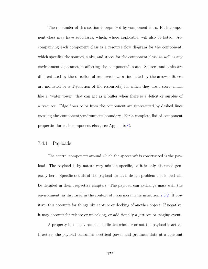
The remainder of this section is organized by component class. Each compo-
nent class may have subclasses, which, where applicable, will also be listed. Ac-
companying each component class is a resource flow diagram for the component,
which specifies the sources, sinks, and stores for the component class, as well as any
environmental parameters affecting the component’s state. Sources and sinks are
differentiated by the direction of resource flow, as indicated by the arrows. Stores
are indicated by a T-junction of the resource(s) for which they are a store, much
like a “water tower” that can act as a buffer when there is a deficit or surplus of
a resource. Edge flows to or from the component are represented by dashed lines
crossing the component/environment boundary. For a complete list of component
properties for each component class, see Appendix C.
7.4.1 Payloads
The central component around which the spacecraft is constructed is the pay-
load. The payload is by nature very mission specific, so it is only discussed gen-
erally here. Specific details of the payload for each design problem considered will
be detailed in their respective chapters. The payload can exchange mass with the
environment, as discussed in the context of mass increments in section 7.3.2. If pos-
itive, this accounts for things like capture or docking of another object. If negative,
it may account for release or unlocking, or additionally a jettison or staging event.
A property in the environment indicates whether or not the payload is active.
If active, the payload consumes electrical power and produces data at a constant
172
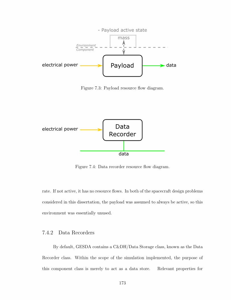
Payload
- Payload active state
dataelectrical power
Envrionment
Component
mass
Figure 7.3: Payload resource flow diagram.
Data
Recorder
data
electrical power
Figure 7.4: Data recorder resource flow diagram.
rate. If not active, it has no resource flows. In both of the spacecraft design problems
considered in this dissertation, the payload was assumed to always be active, so this
environment was essentially unused.
7.4.2 Data Recorders
By default, GESDA contains a C&DH/Data Storage class, known as the Data
Recorder class. Within the scope of the simulation implemented, the purpose of
this component class is merely to act as a data store. Relevant properties for
173

the simulation of this component class are as detailed in Table 7.6. All properties
listed in the table are properties of components of the class. For data recorders,
Table 7.6: Data recorder properties.
property description units
Preq operating power WCdata data capacity bRread data read rate bpsRwrite data write rate bps
fmin,data = 0 (the minimum fill level of a data store is 0 b), and the fmax,data = Cdata
(the maximum fill level of the data store is the component’s data capacity). Within
GESDA, data recorders are assumed to only consume power when reading or writing
data. Therefore their state does not change during the regular component update.
Only on the store update step.
When, δdata > 0, there is a surplus of data, the data recorder sinks data,
assuming its data reservoir is not full. The component level simulation for a data
recorder sinking data follows the process shown in Fig. 7.5. The update returns
r, the remaining portion of δdata that could not be consumed by the component,
and the time tactive it spent during the timestep sinking data up to a maximum of
∆ti, the length of the current timestep. A check is first performed to ensure the
component’s data reservoir is not already full (fc,data = fmax,data = Cdata). If it is,
null outputs indicated in Fig. 7.5 are returned. tactive = 0 indicates the component
was not active during the timestep, and r = δdata indicates no change in the net
flow performed by the component. If the reservoir is not full, the data flowrate rb
174

Start
reservoir
full?
return t = 0,
r = data
yes
no
rb = Rwrite?yes
all data
surplus sunk?
(r=0?)
rb = min(data, Rwrite)tactive= t i
r = data - Rwrite
yes
rb = data
no
tactive= t i
r = 0 data
Rwrite
rb = Rwrite? rb = data
no
tactive= t i
r = rdata - r
Rwrite
r = data - (Rwrite - r)
tactive= t i r
Rwrite
no
yes
Figure 7.5: Data recorder store update process for data surplus.
175

into the component is set to the minimum of δdata and Rwrite. In the case of the
former, the maximum write rate to the component is greater than the net flow rate
of data, so all data surplus can be captured by this component. In the case of the
latter, the data flow into the component is write-limited, so the component alone
will not be sufficient to sink the net data flow. The remainder r of the net flow will
be returned, potentially to be sunk by other stores.
The above is true assuming fc,data < Cdata. This may be true at the beginning
of the timestep, but the component’s data may still become full before the end of
timestep. If this occurs, an additional remainder ∆r must be added to r from above.
For the purpose of calculating remaining r, the remainder of δdata is averaged over
the entire timestep. However, for the purpose of calculating power consumption of
the component while writing, it is assumed to write at a rate Rwrite, for only a time
tactive, which is some fraction of ∆ti.
The combination of rb being set to either Rwrite or δdata and whether or not
the data reservoir becomes full during the current timestep produces four cases, all
with different potential values for r and tactive. Fig. 7.5 gives the logic for selecting
the proper case, and the values of r and tactive in each case.
When δdata < 0, there is a “deficit” of data. Physically, observing our general
spacecraft topology in Fig. 7.1, this means that the spacecraft is transmitting data
out of the system, and there is excess capacity to send any data in recorders. The
recorder sources data from its reservoir until the deficit is eliminated or the reservoir
is empty. The update returns r, the remaining capacity in δdata after sourcing the
component’s data to the system, and the time t it spent during the timestep sourcing
176
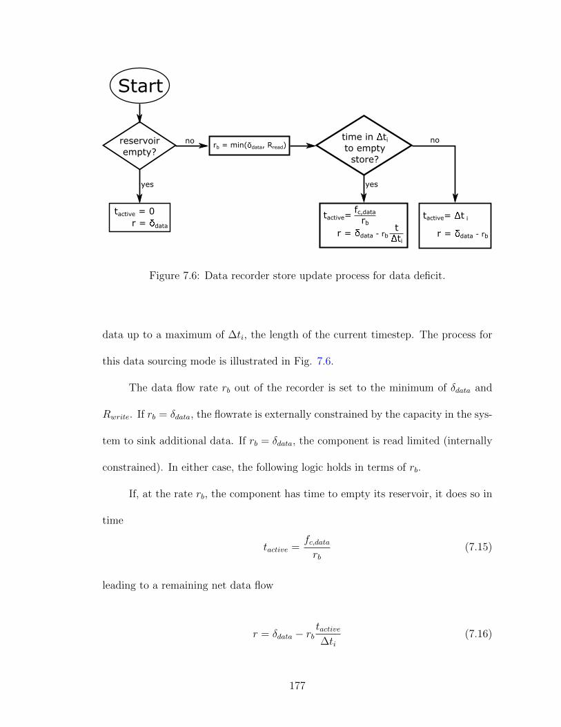
Start
reservoir
empty?
tactive = 0
yes
no time in ti
to empty
store?
rb = min(data, Rread)
r = data
yes
tactive= fc,data
rbtti
r = data - rb
tactive= t i
r = data - rb
no
Figure 7.6: Data recorder store update process for data deficit.
data up to a maximum of ∆ti, the length of the current timestep. The process for
this data sourcing mode is illustrated in Fig. 7.6.
The data flow rate rb out of the recorder is set to the minimum of δdata and
Rwrite. If rb = δdata, the flowrate is externally constrained by the capacity in the sys-
tem to sink additional data. If rb = δdata, the component is read limited (internally
constrained). In either case, the following logic holds in terms of rb.
If, at the rate rb, the component has time to empty its reservoir, it does so in
time
tactive =fc,datarb
(7.15)
leading to a remaining net data flow
r = δdata − rbtactive∆ti
(7.16)
177

In case where tactive = ∆ti, the component uses the full capacity δdata, so r =
δdata − rb. The component will not be able to source all data stored data, only the
portion ∆fc,data = rb∆ti.
A data recorder requires electrical power as long as it is sourcing or sinking
data, at the constant rate Preq. With this in mind, the rate at which a recorder
sinks electrical power is
Pin = Preqtactive (7.17)
Given the appropriate definition of tactive for the current state of the data recorder,
determined following the logic of this subsection, Eq. 7.17 holds regardless of the
state of the component.
7.4.3 RF Modules
RF modules are the sole implementation of a module class within the design
problems considered in this dissertation. The general resource flow of an RF module,
as well as its interaction with the environment, is outlined in Fig. 7.7. RF
modules contain two subcomponent classes; amplifiers and antennas. Amplifiers
and antennas can themselves be broken down into subclasses which function the
same externally, but are modeled differently internally. Amplifier subclasses include
traveling wave tube amplifiers (TWTAs) and solid state transmitters. Antenna
subclasses include low gain antennas (LGAs) and high gain antennas (HGAs). The
hierarchy of RF modules, subcomponent classes, and subcomponent subclasses, is
given in Fig. 7.8.
178

RF Module
- Available terminals - G/T
- distance
- elevation
data
electrical power
Envrionment
Component
telemetry
Figure 7.7: RF module resource flow diagram.
RF Moduleamplifiers antennas
LGAs
HGAssolid state
transmitters
TWTAs
subcla
ss
subcom
ponent c
lass
module
Figure 7.8: RF module subcomponent and subclass hierarchy.
179
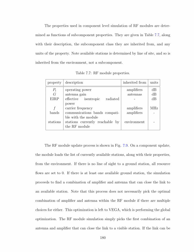
The properties used in component level simulation of RF modules are deter-
mined as functions of subcomponent properties. They are given in Table 7.7, along
with their description, the subcomponent class they are inherited from, and any
units of the property. Note available stations is determined by line of site, and so is
inherited from the environment, not a subcomponent.
Table 7.7: RF module properties.
property description inherited from units
Pt operating power amplifiers dBG antenna gain antennas dB
EIRP effective isentropic radiatedpower
- dB
f carrier frequency amplifiers MHzbands communications bands compati-
ble with the moduleamplifiers -
stations stations currently reachable bythe RF module
environment -
The RF module update process is shown in Fig. 7.9. On a component update,
the module loads the list of currently available stations, along with their properties,
from the environment. If there is no line of sight to a ground station, all resource
flows are set to 0. If there is at least one available ground station, the simulation
proceeds to find a combination of amplifier and antenna that can close the link to
an available station. Note that this process does not necessarily pick the optimal
combination of amplifier and antenna within the RF module if there are multiple
choices for either. This optimization is left to VEGA, which is performing the global
optimization. The RF module simulation simply picks the first combination of an
antenna and amplifier that can close the link to a visible station. If the link can be
180
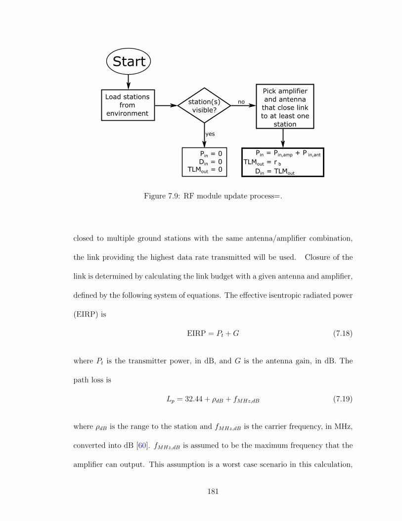
Start
station(s)
visible?
Pin = 0
yes
noLoad stations
from
environment
Din = 0TLMout = 0
Pick amplifier
and antenna
that close link
to at least one
station
Pin = Pin,amp + P in,ant
Din = TLMout
TLMout = r b
Figure 7.9: RF module update process=.
closed to multiple ground stations with the same antenna/amplifier combination,
the link providing the highest data rate transmitted will be used. Closure of the
link is determined by calculating the link budget with a given antenna and amplifier,
defined by the following system of equations. The effective isentropic radiated power
(EIRP) is
EIRP = Pt +G (7.18)
where Pt is the transmitter power, in dB, and G is the antenna gain, in dB. The
path loss is
Lp = 32.44 + ρdB + fMHz,dB (7.19)
where ρdB is the range to the station and fMHz,dB is the carrier frequency, in MHz,
converted into dB [60]. fMHz,dB is assumed to be the maximum frequency that the
amplifier can output. This assumption is a worst case scenario in this calculation,
181

maximizing path loss. The final bitrate transmitted, in dB, is then
rb = EIRP +G/T − kb − Lp − Eb/No (7.20)
where G/T is the gain-to-noise-temperature of the receiving station antenna, kb is
the Boltzmann constant, expressed in dB, assumed to have a value of -228.599 dB,
and Eb/No is the energy per bit to noise power ratio.
Eq. 7.20 gives rb, the rate at which data is transmitted to the environment.
It therefore defines the telemetry flowrate out of the RF module:
TLMout = rb (7.21)
The RF module consumes data as fast as it can modulate it for transmission as
telemetry. Therefore the sink rate of data is equal to the source rate of telemetry:
Din = TLMout (7.22)
Finally, the operating power for the RF module is the sum of the operating power
of the active antenna and amplifier:
Pin = Pin,ant + Pin,amp (7.23)
The remainder of this subsection details the inner workings of the antenna and
amplifier subcomponent classes, giving insight into how Pt and G are determined.
182

7.4.3.1 Amplifiers
Each amplifier has a minimum and maximum output frequency for its carrier
signal, fmin and fmax respectively. These can be user specified in the component
data. Alternatively, a number of compatible IEEE radio frequency bands may be
specified [61]. If bands are specified, fmin and fmax are set to the outer bounds of
the union of the compatible bands.
For TWTAs, the input parameters given in 7.8 were specified for each compo-
nent in the TWTA component library. For a full list of components considered, see
Appendix C. ηT then defines the amplifier’s output power:
Table 7.8: TWTA input parameters.
property description units
fmin minimum carrier frequency Hzfmax maximum carrier frequency HzPin,amp amplifier input power WηT amplifier efficiency -
Pt = ηTPin,amp (7.24)
Solid state transmitters may have fmin and fmax directly specified, or may use
IEEE bands. Within the scope of this dissertation, a solid state amplifier module was
considered synonymous with a solid state amplifier. Table 7.9. The key difference
between the treatment of TWTAs and solid state amplifiers is that Pt is directly
specified as an input parameter for solid state amplifiers rather than being calculated
183

with a specified efficiency. Additionally, solid state amplifiers specify a maximum
data rate, which cannot be exceeded even if link budget analysis would allow it.
Table 7.9: Solid state amplifier input parameters.
property description units
fmin minimum carrier frequency Hzfmax maximum carrier frequency Hz
bands compatible IEEE radio bands -Pin,amp amplifier input power WPt amplifier output power W
rb,max max data throughput rate bps
7.4.3.2 Antennas
Table 7.10 gives the input parameters for LGAs. The only real internal logic
rather than encapsulating these parameters, accessible to the RF module, is that a
check is performed to ensure that there is a range of interoperability between carrier
wavelength of the amplifier and antenna. If there is not a range of interoperability,
a component level constraint violation is noted, to be used in feasibility analysis and
penalty calculation on the spacecraft level.
Table 7.10: LGA input parameters.
property description units
fmin minimum carrier frequency Hzfmax maximum carrier frequency HzG antenna gain dB
Pin,ant antenna input power W
Table 7.11 gives the input parameters for HGAs. In comparison to LGAs, the
184

Table 7.11: HGA input parameters.
property description units
Gnom nominal antenna gain dBλnom nominal wavelength md antenna diameter m
Pin,ant antenna input power WBW half power beamwidth deg
gain now becomes a nominal gain Gnom, with G being sensitive to the wavelength of
the carrier. fmin and fmax are set to ±5% of the nominal carrier wavelength λnom:
fmin = 0.95c
λnom(7.25)
fmin = 1.05c
λnom(7.26)
where c is the speed of light, assumed to be 3 × 10⁸ m/s. While the actual gain
G is not necessarily equal to Gnom, it is assumed to be so. This is because the
frequency range has been bounded based on the nominal wavelength of the antenna,
so component level constraints on the carrier frequency should ensure that λ ≈ λnom.
Pointing requirements were considered beyond the scope of this work, since attitude
control is not modeled. However, for future use, beam width was allowed as an
input parameter, and, if unspecified, was calculated for HGAs:
BW = 70λ
d(7.27)
where λ is the actual wavelength of the carrier.
185

PVA electrical power
Envrionment
Component
solar flux
Figure 7.10: PVA resource flow diagram.
7.4.4 Power Generation
The only power generation type considered was photovoltaic arrays (PVAs).
Future work can investigate use of alternative power generation, including other
forms of solar power, radioisotope power sources, and fusion and fission reactors.
The resource flow for a PVA is given in Fig. 7.10, and their input parameters are
given in Table 7.12. PVAs are perhaps the simplest component class considered.
Table 7.12: PVA input parameters.
property description units
A solar array area m2
ηPV A effective efficiency -
They sink solar flux Φsol from the environment at a fixed rate per unit area, and
have some total solar flux consumed over a set area. Their output power is then
186
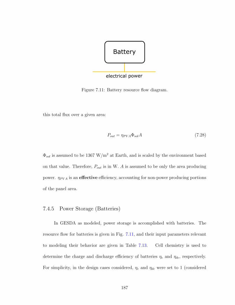
Battery
electrical power
Figure 7.11: Battery resource flow diagram.
this total flux over a given area:
Pout = ηPV AΦsolA (7.28)
Φsol is assumed to be 1367 W/m2 at Earth, and is scaled by the environment based
on that value. Therefore, Pout is in W. A is assumed to be only the area producing
power. ηPV A is an effective efficiency, accounting for non-power producing portions
of the panel area.
7.4.5 Power Storage (Batteries)
In GESDA as modeled, power storage is accomplished with batteries. The
resource flow for batteries is given in Fig. 7.11, and their input parameters relevant
to modeling their behavior are given in Table 7.13. Cell chemistry is used to
determine the charge and discharge efficiency of batteries ηc and ηdc, respectively.
For simplicity, in the design cases considered, ηc and ηdc were set to 1 (considered
187

Table 7.13: Battery input parameters.
property description units
cell chemistry battery cell chemistry -Qmax capacity Whrsd self-discharge rate %/dayηc battery charging efficiency -ηdc battery discharge efficiency -
a reasonable approximation at this design stage, assuming a lithium ion or lithium
polymer cell chemistry, which all batteries considered were). Consideration of non-
unity values for ηc and ηdc is included in the model for generality. A nominal depth
of discharge of 20% was set for batteries. On the regular component update, self-
discharge is applied to the battery:
fc,i = fc,i−1(1− rsd)∆ti/86400 s (7.29)
where fc,i is the fill level of the battery’s electrical power reservoir at the current
timestep (after applying self-discharge), fc,i−1 is the fill level before applying self
discharge, and ∆ti is the duration of the timestep. Eq. 7.29 takes the self discharge
rate in %/day, converts it to percent over the duration ∆ti, and applies it to the
battery fur the current timestep. The remainder of battery functionality occurs
during the store update step of the simulation.
When δpower > 0, there is a surplus of electrical power in the system, and the
battery will charge. Some power will be lost during charging for ηc < 1. To increase
the energy stored in the battery by ∆fc, the battery must actually sink amount of
188

energy equal to ∆fcηc
. To account for this, when sinking power to the battery, the
power available to the reservoir is considered to actually be ηcδpower. The remainder
r of δc not sinked by the battery is then calculated as follows. Consider ηc to be due
to the internal resistance of the battery. The total energy consumed by the battery
over time t is
Etot,sink = ∆fc +Qh (7.30)
where ∆fc is the change in energy level of the battery’s power reservoir (i.e. energy
that becomes stored in the battery), and Qh, the energy that is dissipated as heat.
Following the same logic as discussed for data recorders, t is defined as the time
during the timestep ∆ti during which the battery is charging. Dividing then by t,
the power sinked to the battery can be similarly defined as a change in the net flow
of electrical power:
∆δpower =∆fct
+ Qh (7.31)
ηc defines the ratio of ∆δpower that actually makes it into the battery. Since, by
definition,
∆fct
= ∆δpowerηc, (7.32)
it follows that
∆δpower =∆fctηc
(7.33)
189

The maximum charge of the battery is fmax = Qmax, defined as a parameter of each
battery. The maximum amount by which the battery can then be charged is then
∆fmax = fmax − fc (7.34)
For δpowerηc∆ti < ∆fmax, the battery consumes the entire net flow, returning a
remainder of r = 0. The actual change in the charge in the reservoir is
∆f = δpowerηc∆ti (7.35)
For δpowerηc∆ti > ∆fmax, the battery becomes fully charged during this timestep
without consuming the full power surplus. In this case, from Eq. 7.33, the decrease
portion of the power surplus consumed is
∆δpower =∆fmax∆tiηc
(7.36)
The remainder of the power surplus, available to charge other power stores, is then
r = δpower −∆δpower (7.37)
When δpower < 0, there is a power deficit within the system. The battery will
supplement power generation in the system by sourcing power from its reservoir.
Like charging the battery, some power drawn from the battery will be lost for ηdc < 1.
Over ∆ti, the energy that must be drained from the battery to compensate a power
190
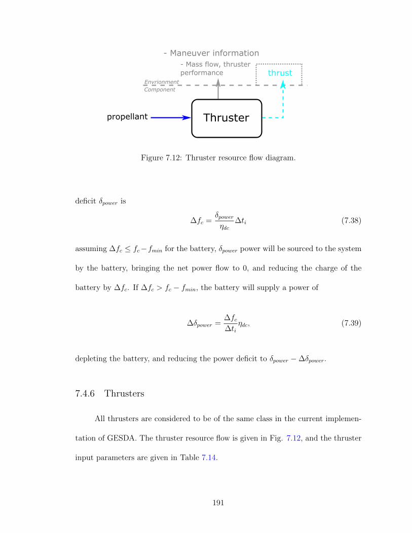
Thruster
- Maneuver information
propellant
Envrionment
Component
thrust- Mass flow, thruster
performance
Figure 7.12: Thruster resource flow diagram.
deficit δpower is
∆fc =δpowerηdc
∆ti (7.38)
assuming ∆fc ≤ fc−fmin for the battery, δpower power will be sourced to the system
by the battery, bringing the net power flow to 0, and reducing the charge of the
battery by ∆fc. If ∆fc > fc − fmin, the battery will supply a power of
∆δpower =∆fc∆ti
ηdc, (7.39)
depleting the battery, and reducing the power deficit to δpower −∆δpower.
7.4.6 Thrusters
All thrusters are considered to be of the same class in the current implemen-
tation of GESDA. The thruster resource flow is given in Fig. 7.12, and the thruster
input parameters are given in Table 7.14.
191

Table 7.14: Thruster input parameters.
property description units
Isp specific impulse sFt thrust nPon operating power WPoff standby power Wprop1 propellant #1 type -prop2 propellant #2 type -f1 mass fraction of propellant 1 -f2 mass fraction of propellant 2 -
Each thruster has an associated specific impulse and thrust, supplied as input
parameters. From these, the mass flowrate is defined as
m =FtIspg
(7.40)
where g is the gravitational acceleration at the surface of the Earth, assumed to be
9.81 m/s2. For any bipropellant thrusters, (those for which prop2 is defined), this
mass flowrate is divided into a mass flowrate for each propellant by the ratio of the
propellant mass fractions:
m1 = mf1
f1 + f2
(7.41)
m2 = mf2
f1 + f2
(7.42)
Thrusters are perhaps the most complex component class included. In simu-
lation, at any given timestep, there is a desired ∆V to perform. ∆V will be some
portion of the current maneuver set in the environment. Specifically, it will be the
portion of the current maneuver that is still to be completed at the beginning of the
192
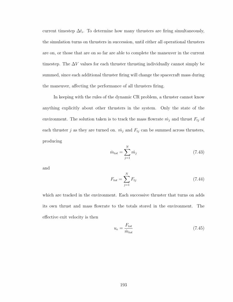
current timestep ∆ti. To determine how many thrusters are firing simultaneously,
the simulation turns on thrusters in succession, until either all operational thrusters
are on, or those that are on so far are able to complete the maneuver in the current
timestep. The ∆V values for each thruster thrusting individually cannot simply be
summed, since each additional thruster firing will change the spacecraft mass during
the maneuver, affecting the performance of all thrusters firing.
In keeping with the rules of the dynamic CR problem, a thruster cannot know
anything explicitly about other thrusters in the system. Only the state of the
environment. The solution taken is to track the mass flowrate mj and thrust Ftj of
each thruster j as they are turned on. mj and Ftj can be summed across thrusters,
producing
mtot =N∑j=1
mj (7.43)
and
Ftot =N∑j=1
Ftj (7.44)
which are tracked in the environment. Each successive thruster that turns on adds
its own thrust and mass flowrate to the totals stored in the environment. The
effective exit velocity is then
ue =Ftotmtot
(7.45)
193
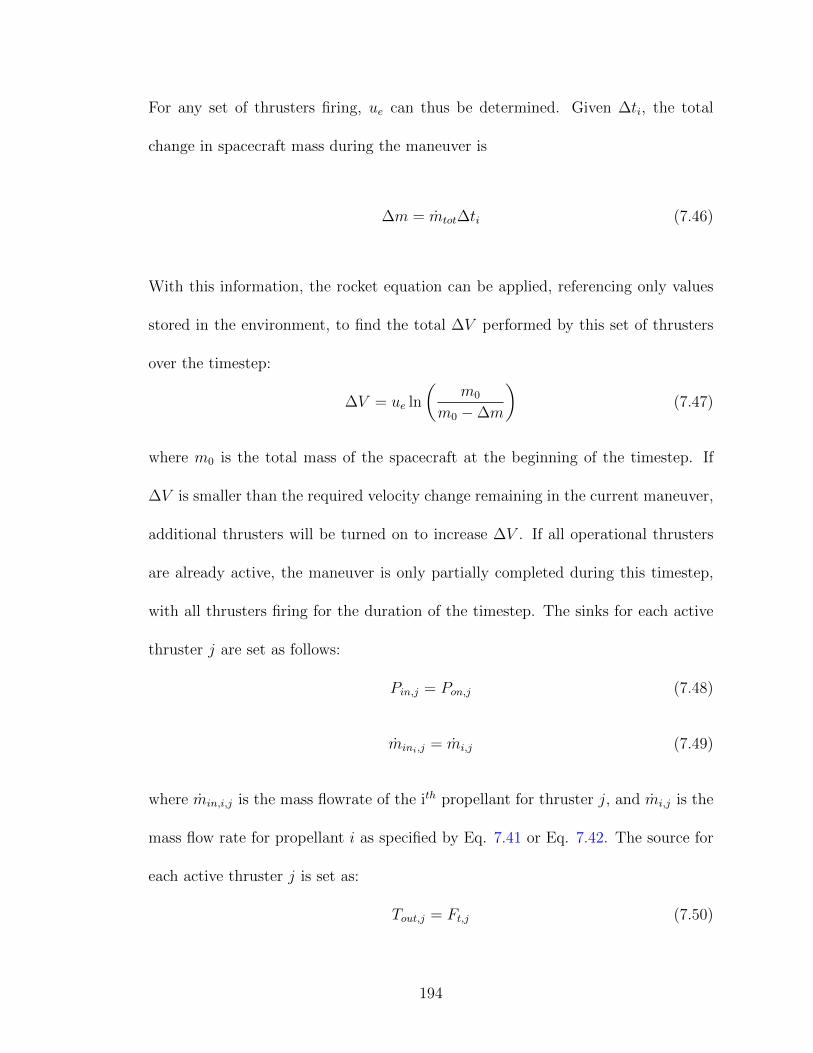
For any set of thrusters firing, ue can thus be determined. Given ∆ti, the total
change in spacecraft mass during the maneuver is
∆m = mtot∆ti (7.46)
With this information, the rocket equation can be applied, referencing only values
stored in the environment, to find the total ∆V performed by this set of thrusters
over the timestep:
∆V = ue ln
(m0
m0 −∆m
)(7.47)
where m0 is the total mass of the spacecraft at the beginning of the timestep. If
∆V is smaller than the required velocity change remaining in the current maneuver,
additional thrusters will be turned on to increase ∆V . If all operational thrusters
are already active, the maneuver is only partially completed during this timestep,
with all thrusters firing for the duration of the timestep. The sinks for each active
thruster j are set as follows:
Pin,j = Pon,j (7.48)
mini,j = mi,j (7.49)
where min,i,j is the mass flowrate of the ith propellant for thruster j, and mi,j is the
mass flow rate for propellant i as specified by Eq. 7.41 or Eq. 7.42. The source for
each active thruster j is set as:
Tout,j = Ft,j (7.50)
194

If ∆V exceeds the required velocity change remaining for the current maneu-
ver, the required change in mass to complete the maneuver is calculated:
∆mreq = m0
(e−∆V/ue − 1
)(7.51)
The portion of ∆ti required to complete the maneuver is then calculated as
t =∆mreq
mtot
(7.52)
and the above sources and sinks for each thruster are scaled by the portion of ∆ti
required:
Pin,j = Pon,jt
∆ti(7.53)
mini,j = mi,jt
∆ti(7.54)
Tout,j = Ft,jt
∆ti(7.55)
The logic stated above is for nonimpulsive maneuvers, where it is expected
that the entire duration of each orbit may be used for maneuvering. For impulsive
maneuvers, it is assumed that only 10% of each orbit may be used for maneuvering.
As a result, the same ∆V will take longer to perform, but for any given timestep, the
above equations hold by replacing ∆ti with 0.1∆ti. Note that no explicit check is
performed to determine if impulsive or low thrust maneuvers are more appropriate
for a given thruster. That selection is made for the entire spacecraft by the L1
genome, and thus is part of the global optimization. There is therefore an implicit
195

relationship between the types of thrusters used by the spacecraft and the maneuver
regime. Impulsive maneuvers are preferable, but the time required to complete them
will become prohibitively long for low thrust systems.
Fig. 7.13 details the update process for thrusters, as currently implemented.
It is hoped that this illustration of the logic described above may make the textual
description itself be more clear. There are some algebraic differences between the
above explanation and the figure. These are simplifications in the text for clarity,
and the end results are the same. Where there is a discrepancy, the figure describes
the process as implemented in GESDA.
Within Fig. 7.13, ∆V represents the ∆V remaining in the environment’s ∆V
store at the beginning of the timestep. ∆Vp represents the ∆V performed over
∆ti by the currently active thrusters. Assuming the maneuver has not already
been completed with earlier thrusters, and that some amount of all propellant types
required for this thruster is present on the spacecraft, the thruster is activated. Its
mass flowrate and thrust are added to the totals, stored in the environment. ue
and t are calculated based on Eq. 7.45 and Eq. 7.52, respectively. If the maneuver
is impulsive, ∆t is set 10% of ∆ti, the timestep duration. If it is not impulsive,
∆t = ∆ti. The thruster is then activated, and a check is performed to determine
if the maneuver can now be completed on this timestep. If so, ∆Vp is set to ∆V ,
and the resource flows are set for each active thruster following Eqs. 7.53, 7.54, and
7.55.
If the maneuver cannot be completed on this timestep, the resource flows are
set following Eqs. 7.48, 7.49, and 7.50. If the maneuvers are impulsive, each of
196
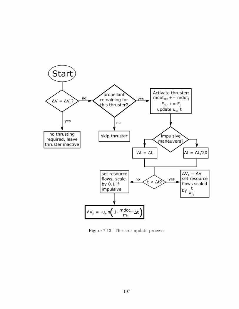
Start
propellant
remaining for
this thruster?
no
yes
V = Vp?
no
impulsive
maneuvers?
no thrusting
required, leave
thruster inactive
skip thruster
Activate thruster:mdottot += mdotj
Ftot += Fj
update ue, t
yes
t = ti t = ti/20
t < t?
Vp = V
set resource
flows scaled t
ti
by
yes
set resource
flows, scale
by 0.1 if
impulsive
no
Vp = -ueln mdottot
m0
t)(1-
Figure 7.13: Thruster update process.
197
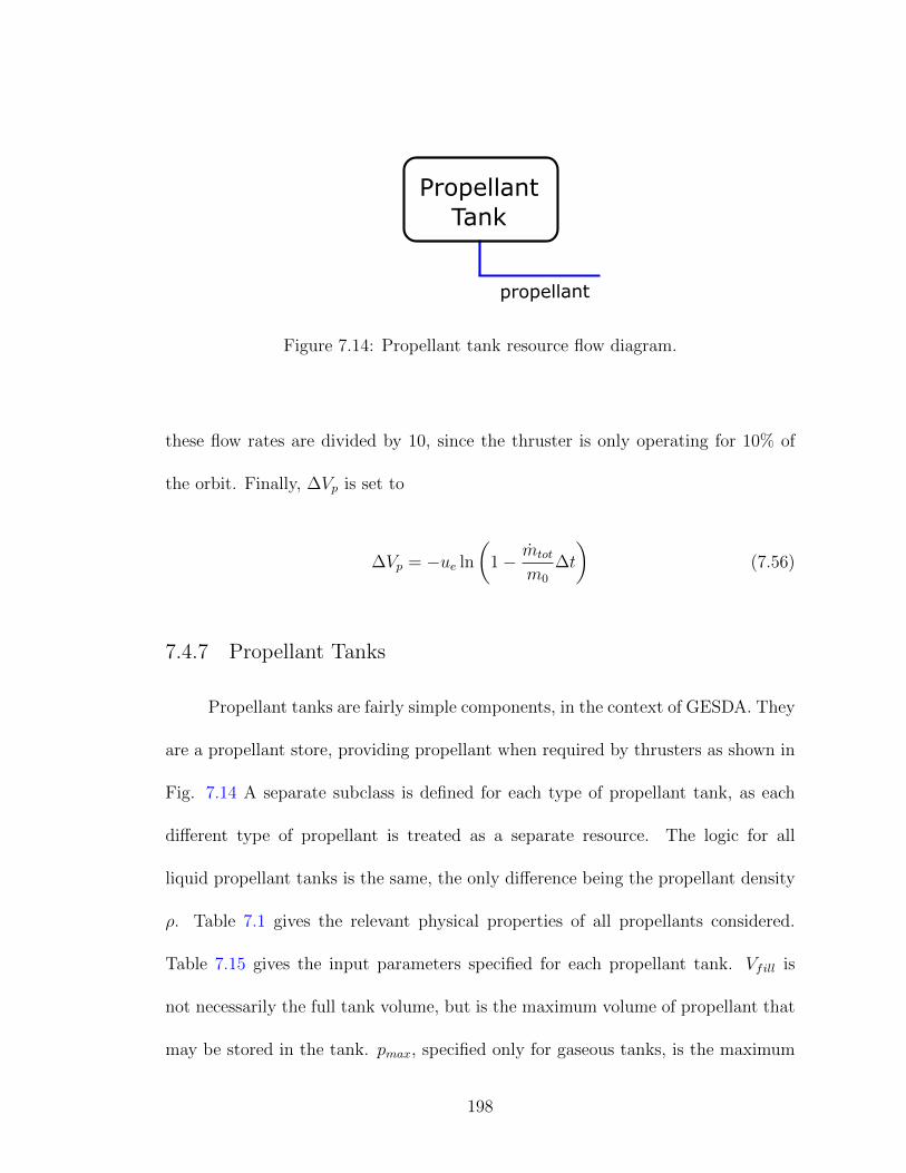
Propellant
Tank
propellant
Figure 7.14: Propellant tank resource flow diagram.
these flow rates are divided by 10, since the thruster is only operating for 10% of
the orbit. Finally, ∆Vp is set to
∆Vp = −ue ln
(1− mtot
m0
∆t
)(7.56)
7.4.7 Propellant Tanks
Propellant tanks are fairly simple components, in the context of GESDA. They
are a propellant store, providing propellant when required by thrusters as shown in
Fig. 7.14 A separate subclass is defined for each type of propellant tank, as each
different type of propellant is treated as a separate resource. The logic for all
liquid propellant tanks is the same, the only difference being the propellant density
ρ. Table 7.1 gives the relevant physical properties of all propellants considered.
Table 7.15 gives the input parameters specified for each propellant tank. Vfill is
not necessarily the full tank volume, but is the maximum volume of propellant that
may be stored in the tank. pmax, specified only for gaseous tanks, is the maximum
198

Table 7.15: Propellant tank input parameters.
property description units
Vfill fill volume m3
pmax maximum pressure (gaseous tanks only) Pa
pressure of propellant in the tank. All tanks are initialized at their maximum fill
level. Propellant fill level is measured in propellant mass in the tank. For liquid
tanks,
fmax = ρVfill (7.57)
where ρ is the density of the propellant. For gaseous tanks, the density is defined
from the ideal gas law [62]:
ρ =MpmaxRT
× 10−3 (7.58)
where M is the molar mass of the propellant, R is the universal gas constant,
assumed to be 8.314 JmolK
, and T is the tank temperature, assumed to be 300 K.
The factor of 10−3 is a conversion from kg/m3 to kg/L. With ρ in kg/L, we can
calculate the mass of gaseous propellant by Eq. 7.57.
Unlike other component classes, the mass of propellant tanks can change as
they are depleted. At any given time, the mass of a propellant tank is
m = mdry + fc (7.59)
where mdry is the dry mass of the tank, specified as a component parameter as for
all other components, and fc is the current fill level of the tank. Propellant tanks
199
have no behavior during the regular component update. During the store update
step, they source propellant as required for thrusters of their propellant type.
7.5 Summary
In this chapter we have set up the general satellite design problem. The
dynamic CR has been extended with a specific eye on spacecraft design, defining
a general spacecraft topology, as well as an environment for modeling spacecraft
on closed orbits. Additionally, this chapter has defined a set of general component
classes whose applicability spans a wide range of missions. One particular exception
is the design of payloads, which, while spoken about generally here, are by necessity
mission specific. In practice, a tool like GESDA does not design a payload, but
takes one produced by an external design campaign and trades spacecraft designs
around it. The remaining chapters will apply the framework developed thus far
to two actual spacecraft design problems, comparing the results with existing data
from other studies or final flight vehicles, followed by conclusions of this work and
general avenues for future follow-on work.
200

Chapter 8: A Passive Spacecraft Case Study: Earth Observing Cube-
sat
8.1 Overview
In previous chapters, a dynamic CR model and associated multiobjective opti-
mization framework have been developed. These have then been applied to develop
GESDA, a framework for facilitating spacecraft-level trade space analysis. In this
chapter, an example and validation of GESDA is provided for a passive spacecraft
design.
This chapter investigates the design of a spacecraft to perform the Earth ob-
serving mission currently carried out by the Dove spacecraft produced by Planet
Labs [58]. A payload is developed based on what is publicly known about Planet’s
Dove spacecraft. A trade study is then performed using GESDA to maximize the
data returned by a single spacecraft supporting the Dove payload while minimizing
the spacecraft mass. Finally, the results are compared with the details known of
actual flown Dove cubesats.
201
8.2 The Dove Spacecraft and Payload
The Dove is a class of Earth imaging 3U cubesats under development by and
flown by Planet, Inc [63]. Planet has been a strong proponent of “agile aerospace,”
applying the principles of agile software development [64] to spacecraft design. In
this context agile aerospace stresses a focus on rapid turnaround and incremental
improvement through continuous tweaking of a design, and getting by with “min-
imal documentation.” The use of agile development by Planet has been facilitated
by the advent of capable, inexpensive cubesats, and a dramatic reduction in the
cost to launch them [65, 66]. Unfortunately, the lack of focus on documentation
associated with agile aerospace, combined with the proprietary and incrementally
changing nature of the Dove payload, makes it hard to fully pin down payload spec-
ifications. The payload design used for this case study, as detailed below, is an
attempt to reverse engineer PlanetScope 2 (PS2), the Dove 3 payload, from what
data is available, based primarily on the Planet Labs Specifications document [63].
The payload resource flow is the same as specified by Fig. 7.3, with the
exception that this is a passive spacecraft. As a result, no mass is exchanged with
the environment. The payload is assumed to continuously operate, so the active
state information from the orbit is not used. Therefore, the payload simply sources
data and sinks electrical power, both at a constant rate.
Each Dove spacecraft is assumed to be in a 475 km circular sun-synchronous
orbit, as specified for future Dove launches [63]. The orbit crosses the equator at
10:30 am local time, defining the right ascension Ω of the orbit to be 250.6. At this
202
altitude, the spacecraft is assumed to have a ground sampling distance (resolution) of
3.7 m, and the imager has a field of view of 24.6×16.4 km. Combining these leads to
an image size of approximately 6650×4440 pixels, or 30 megapixels (MP) per image.
Images are captured in 12 bits per pixel onboard the spacecraft. According to [63],
they are compressed for transmission, but for the purposes of payload development,
12 bits per pixel was assumed since this is the relevant number for the data flow
from the payload. This leads to an image size of 360 Mb per image.
Planet downlinks 1.3 million images per day from 160 satellites [67]. This leads
to a downlink of 8125 images per day per satellite. Assuming continuous imaging,
this corresponds to one image every ten seconds. Taking this imaging rate, and the
360 Mb image size, the payload considered here is assumed to produce data at a
rate of 36 Mbps.
No power consumption or strict mass data for the imager itself was found in
existing literature. It is known that all non-in-house components that Planet uses
are commercial off-the-shelf (COTS) components [68]. Specifically, the detector is
an industrial, 29 MP COTS CCD detector. This matches the description of the
Imperx B6640 [69], which also has approximately the same frame image dimensions
(6600 x 4400 pixels). The detector has a power draw of 7.5 W, so Pin for the payload
was assumed to be 7.5 W. Its mass of 0.37 kg is also very close to the mass of the
PS2 camera as stated in the Dove 3 Orbital Debris Assessment Report (ODAR) [70].
The B6640 also features an internal 2 Gb of data storage, so a data store was added
to the payload.
203

PS2 36 Mbps7.5 W
Figure 8.1: PS2 resource flow diagram.
While it was assumed that the B6640 detector and other electronics were used,
it is known that the optics were different. The PS2 uses a five element optical system,
which consumes most of the internal volume of the 3U x 1U Dove cubesat. Previous
Dove payloads used a Maksutov Cassegrain optical system. From [70], it is known
that the optical tube, assumed to approximate the mass of the optical system, was
2.08 kg. Therefore, the total payload mass is assumed to be 2.45 kg. To summarize,
the payload for this design problem is as shown in Fig. 8.1, and has the parameters
given in Table 8.1. Note that the payload is both a data source and a data store.
As indicated, it produces data at a rate of 36 Mbps, but also has an internal data
reservoir, which is empty at the beginning of the simulation.
Table 8.1: PS2 component parameters.
property description value units
Pin input power 7.5 Wm mass 2.45 kgrb data rate 36× 106 bpsfmax data capacity 2× 10⁹ bps
204
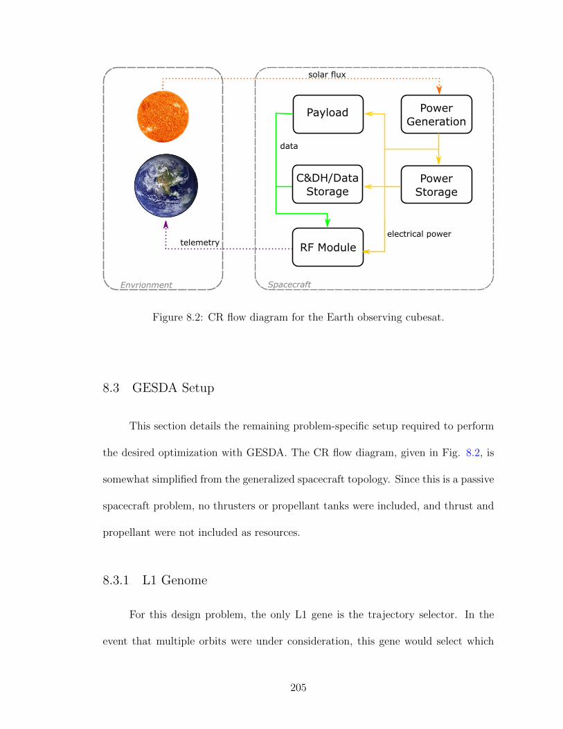
Power
Generation
Power
Storage
C&DH/Data
Storage
Payload
RF Module
SpacecraftEnvrionment
data
telemetry
solar flux
electrical power
Figure 8.2: CR flow diagram for the Earth observing cubesat.
8.3 GESDA Setup
This section details the remaining problem-specific setup required to perform
the desired optimization with GESDA. The CR flow diagram, given in Fig. 8.2, is
somewhat simplified from the generalized spacecraft topology. Since this is a passive
spacecraft problem, no thrusters or propellant tanks were included, and thrust and
propellant were not included as resources.
8.3.1 L1 Genome
For this design problem, the only L1 gene is the trajectory selector. In the
event that multiple orbits were under consideration, this gene would select which
205
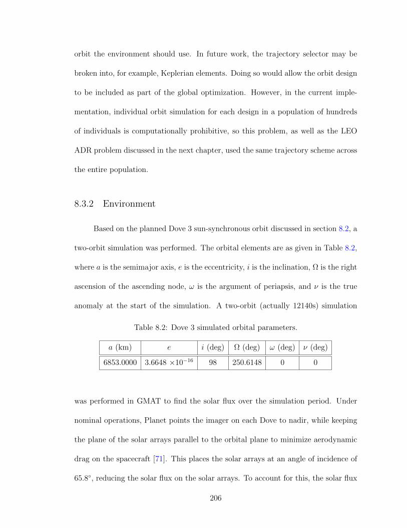
orbit the environment should use. In future work, the trajectory selector may be
broken into, for example, Keplerian elements. Doing so would allow the orbit design
to be included as part of the global optimization. However, in the current imple-
mentation, individual orbit simulation for each design in a population of hundreds
of individuals is computationally prohibitive, so this problem, as well as the LEO
ADR problem discussed in the next chapter, used the same trajectory scheme across
the entire population.
8.3.2 Environment
Based on the planned Dove 3 sun-synchronous orbit discussed in section 8.2, a
two-orbit simulation was performed. The orbital elements are as given in Table 8.2,
where a is the semimajor axis, e is the eccentricity, i is the inclination, Ω is the right
ascension of the ascending node, ω is the argument of periapsis, and ν is the true
anomaly at the start of the simulation. A two-orbit (actually 12140s) simulation
Table 8.2: Dove 3 simulated orbital parameters.
a (km) e i (deg) Ω (deg) ω (deg) ν (deg)
6853.0000 3.6648 ×10⁻¹⁶ 98 250.6148 0 0
was performed in GMAT to find the solar flux over the simulation period. Under
nominal operations, Planet points the imager on each Dove to nadir, while keeping
the plane of the solar arrays parallel to the orbital plane to minimize aerodynamic
drag on the spacecraft [71]. This places the solar arrays at an angle of incidence of
65.8, reducing the solar flux on the solar arrays. To account for this, the solar flux
206

in the simulation was multiplied by a cosine loss factor of 0.41. In other words, in
direct sunlight in Earth orbit, where the incident solar flux would otherwise be 1367
W/m2, the solar flux would instead be 560.5 W/m2.
The same orbit was simulated in STK for communications access calculations,
from 12:00 UTC to 15:00 UTC on January 1, 2000. Planet uses 22 private X-band
ground stations located at eight sites around the world, all providing at least 29
dB/K G/T [67]. Like the case with the payload, many of the details of these ground
stations were unknown, so an attempt was made to develop a comparable setup
in simulation. Additionally, the goal of the simulation and optimization is not to
necessarily provide an identical simulation to the setup that Planet arrived at. It was
to provide a notional simulation of the spacecraft environment for design purposes.
Then, given the PS2 payload a Dove-like design could arise, but the scenario was
not set up to favor it outright.
In the simulation for this design problem, two Near Earth Network ground
stations were available, Troll Satellite Station in Antarctica, and Svalbard Satellite
Station in Svalbard, Norway [59]. By observation of the ground site map in [67],
both appear to actually host Planet ground stations as well. These ground stations,
along with one in northern North America, appear to be strategically placed close
enough to the poles as to have a line of sight to sun synchronous spacecraft on most
orbits, ensuring an abundance of downlink opportunities.
In addition to Troll and Svalbard, one TDRSS satellite, TDRS-3 was included
as a space station (i.e., a “ground station” in space). For TDRS-3, it was assumed for
the scenario that coverage was only available from the start of the simulation, when
207

the spacecraft is already in TDRS-3’s line of sight, until the spacecraft passes beyond
TDRS-3’s line of sight for the first time. This mimics the limited availability of
TDRSS’s S-Band Multiple Access (SMA) service, which is shared among numerous
customers [72]. Table 8.3 gives the available bands and assumed G/T for each
station. For a complete list of access data during the simulation, see Appendix D.
Table 8.3: Downlink station parameters.
station name band G/T (dB/K)
TDRS-3 S 4.5
SvalbardS 20.5X 35.4
TrollS 19.4X 32
8.3.3 Components Used
For this design problem, the payload detailed in section 8.2 was used. Other
component classes used were data recorders, PVAs, batteries, and RF modules,
comprising TWTAs, solid state amplifiers, LGAs, and HGAs. The internal models
for each of these are as described in section 7.4. Since this is a passive satellite
design problem, thrusters and propellant tanks were not included.
For optimization, a constraint of one payload per spacecraft was added as a
component quantity constraint. All other component quantities were unconstrained,
but seed ranges were specified for each class. These are used when initializing the
first generation of designs, but do not constrain the number of components in each
208
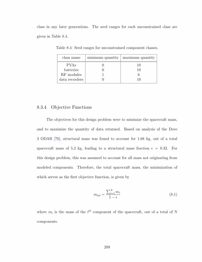
class in any later generations. The seed ranges for each unconstrained class are
given in Table 8.4.
Table 8.4: Seed ranges for unconstrained component classes.
class name minimum quantity maximum quantity
PVAs 0 10batteries 0 10
RF modules 1 6data recorders 0 10
8.3.4 Objective Functions
The objectives for this design problem were to minimize the spacecraft mass,
and to maximize the quantity of data returned. Based on analysis of the Dove
3 ODAR [70], structural mass was found to account for 1.68 kg, out of a total
spacecraft mass of 5.2 kg, leading to a structural mass fraction ε = 0.32. For
this design problem, this was assumed to account for all mass not originating from
modeled components. Therefore, the total spacecraft mass, the minimization of
which serves as the first objective function, is given by
mtot =
∑Ni=1mi
1− ε(8.1)
where mi is the mass of the ith component of the spacecraft, out of a total of N
components.
209
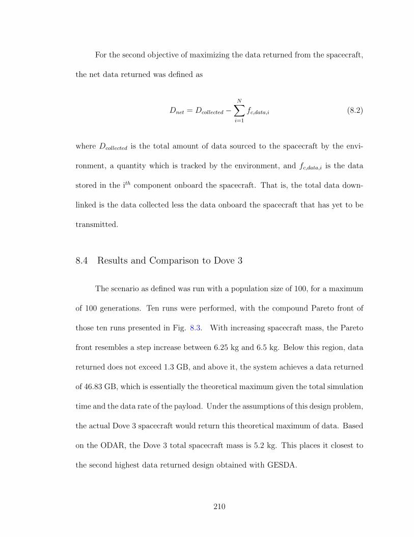
For the second objective of maximizing the data returned from the spacecraft,
the net data returned was defined as
Dnet = Dcollected −N∑i=1
fc,data,i (8.2)
where Dcollected is the total amount of data sourced to the spacecraft by the envi-
ronment, a quantity which is tracked by the environment, and fc,data,i is the data
stored in the ith component onboard the spacecraft. That is, the total data down-
linked is the data collected less the data onboard the spacecraft that has yet to be
transmitted.
8.4 Results and Comparison to Dove 3
The scenario as defined was run with a population size of 100, for a maximum
of 100 generations. Ten runs were performed, with the compound Pareto front of
those ten runs presented in Fig. 8.3. With increasing spacecraft mass, the Pareto
front resembles a step increase between 6.25 kg and 6.5 kg. Below this region, data
returned does not exceed 1.3 GB, and above it, the system achieves a data returned
of 46.83 GB, which is essentially the theoretical maximum given the total simulation
time and the data rate of the payload. Under the assumptions of this design problem,
the actual Dove 3 spacecraft would return this theoretical maximum of data. Based
on the ODAR, the Dove 3 total spacecraft mass is 5.2 kg. This places it closest to
the second highest data returned design obtained with GESDA.
210
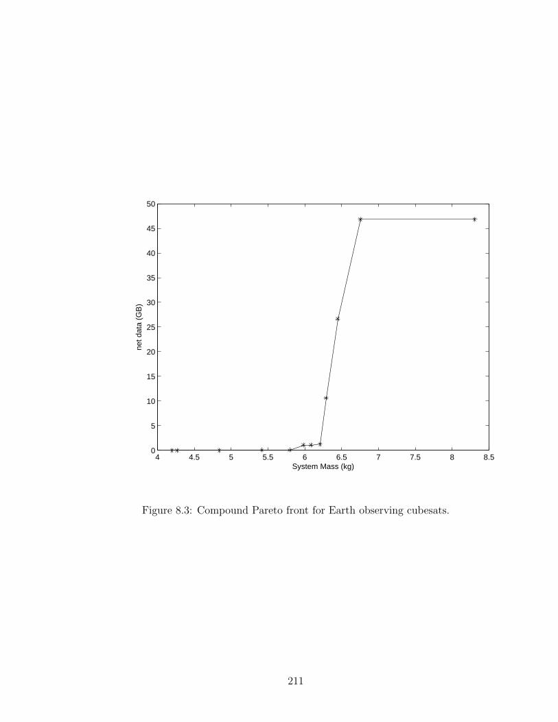
4 4.5 5 5.5 6 6.5 7 7.5 8 8.50
5
10
15
20
25
30
35
40
45
50
System Mass (kg)
net d
ata
(GB
)
Figure 8.3: Compound Pareto front for Earth observing cubesats.
211
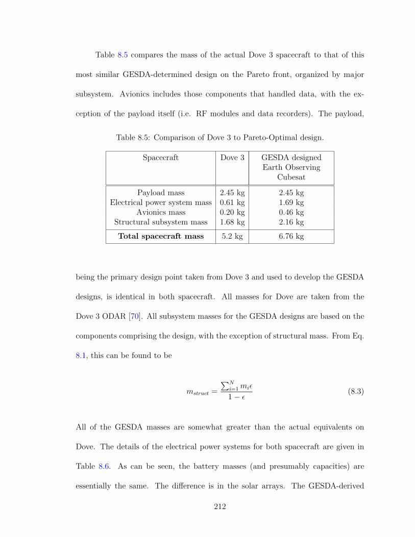
Table 8.5 compares the mass of the actual Dove 3 spacecraft to that of this
most similar GESDA-determined design on the Pareto front, organized by major
subsystem. Avionics includes those components that handled data, with the ex-
ception of the payload itself (i.e. RF modules and data recorders). The payload,
Table 8.5: Comparison of Dove 3 to Pareto-Optimal design.
Spacecraft Dove 3 GESDA designedEarth Observing
Cubesat
Payload mass 2.45 kg 2.45 kgElectrical power system mass 0.61 kg 1.69 kg
Avionics mass 0.20 kg 0.46 kgStructural subsystem mass 1.68 kg 2.16 kg
Total spacecraft mass 5.2 kg 6.76 kg
being the primary design point taken from Dove 3 and used to develop the GESDA
designs, is identical in both spacecraft. All masses for Dove are taken from the
Dove 3 ODAR [70]. All subsystem masses for the GESDA designs are based on the
components comprising the design, with the exception of structural mass. From Eq.
8.1, this can be found to be
mstruct =
∑Ni=1 miε
1− ε(8.3)
All of the GESDA masses are somewhat greater than the actual equivalents on
Dove. The details of the electrical power systems for both spacecraft are given in
Table 8.6. As can be seen, the battery masses (and presumably capacities) are
essentially the same. The difference is in the solar arrays. The GESDA-derived
212

Table 8.6: Electrical power system comparison.
Spacecraft Dove 3 GESDA designedEarth Observing
Cubesat
PVA mass (kg) 0.40 1.09PVA area (cm2) 210 230
Battery mass 0.61 0.60
design has roughly the same solar array area but three times the solar array mass.
A further investigation into the solar arrays used for Dove reveals the likely cause
for the discrepancy. In GESDA’s component library for this design problem, only
space-rated cubesat solar panels were considered. However, Planet uses Triangular
Advanced Solar Cells (TASC) [73, 74]. TASC are intended as terrestrial solar cells,
and, at least in Planet’s implementation, do not have coverglass to protect from the
radiation environment. Studies into the performance of TASCs in the space radiation
environment suggest a degradation to 66% of beginning of life power output after
two years [75]. However, it does mean that they achieve a greater efficiency at the
beginning of their life.
According to [74], a typical TASC cell produces 0.027 W/cm2 in the Dove 3
orbital environment (i.e. 1 Sun). Typically, two TASC cells are arranged into a
rectangle, with each rectangle measuring 4.93 cm2. By observation of pre-launch
imagery, Dove 3 does indeed use TASC, arranged in 3U arrays, with each array
measuring 5 x 8 rectangles. This equates to 40 rectangles per array, which equates
to 197 cm2 per array. Given the rated power per unit area for TASC, this gives a
power of 5.32 W per Dove array at beginning of life. Given that each Dove 3 has 7
213
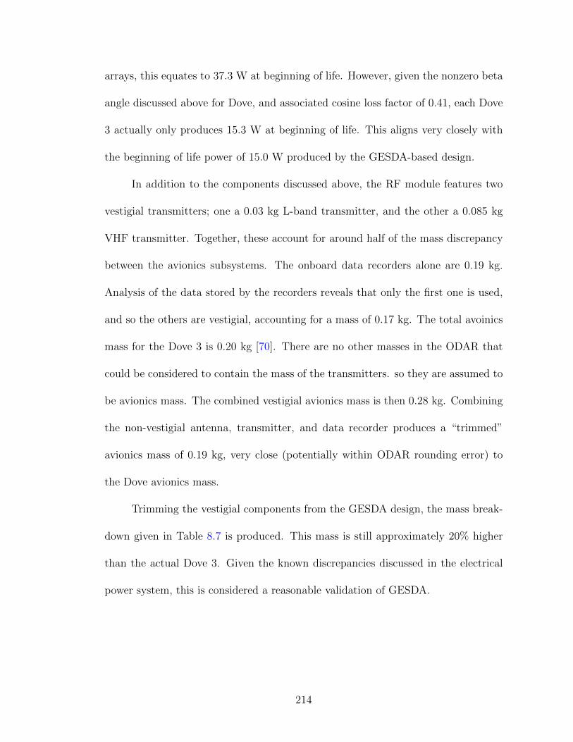
arrays, this equates to 37.3 W at beginning of life. However, given the nonzero beta
angle discussed above for Dove, and associated cosine loss factor of 0.41, each Dove
3 actually only produces 15.3 W at beginning of life. This aligns very closely with
the beginning of life power of 15.0 W produced by the GESDA-based design.
In addition to the components discussed above, the RF module features two
vestigial transmitters; one a 0.03 kg L-band transmitter, and the other a 0.085 kg
VHF transmitter. Together, these account for around half of the mass discrepancy
between the avionics subsystems. The onboard data recorders alone are 0.19 kg.
Analysis of the data stored by the recorders reveals that only the first one is used,
and so the others are vestigial, accounting for a mass of 0.17 kg. The total avoinics
mass for the Dove 3 is 0.20 kg [70]. There are no other masses in the ODAR that
could be considered to contain the mass of the transmitters. so they are assumed to
be avionics mass. The combined vestigial avionics mass is then 0.28 kg. Combining
the non-vestigial antenna, transmitter, and data recorder produces a “trimmed”
avionics mass of 0.19 kg, very close (potentially within ODAR rounding error) to
the Dove avionics mass.
Trimming the vestigial components from the GESDA design, the mass break-
down given in Table 8.7 is produced. This mass is still approximately 20% higher
than the actual Dove 3. Given the known discrepancies discussed in the electrical
power system, this is considered a reasonable validation of GESDA.
214
Table 8.7: Comparison of Dove 3 to Pareto-Optimal design.
Spacecraft Dove 3 GESDA designedEarth Observing
Cubesat
Payload mass 2.45 kg 2.45 kgElectrical power system mass 0.61 kg 1.69 kg
Avionics mass 0.20 kg 0.17 kgStructural subsystem mass 1.68 kg 2.03 kg
Total spacecraft mass 5.2 kg 6.3 kg
8.5 Summary
In this chapter we have demonstrated the use of GESDA for passive spacecraft
trade space exploration. In comparing the results obtained to an actual flown mis-
sion carrying the same payload, this chapter serves as a validation of the CR model
and GESDA. It is likely that further analysis and refinement of the simulation could
produce closer results to the actual Dove 3 spacecraft. However, the results obtained
do validate the framework, and further refinement would come with an increase in
complexity, and likely computational requirements. It is therefore left for future
work in some later revision of GESDA.
215
Chapter 9: Revisiting LEO ADR: An Active Spacecraft Case Study
9.1 Overview
Ultimately, we have arrived back at the original LEO active debris removal
(ADR) design problem which was originally considered in Chap. 2, and which largely
motivated the development of GESDA, detailed throughout this dissertation up to
this point. As a final validation, GESDA is now used to repeat the design study
of Chap. 2. As such, many of the implementation decisions for this design case
were made to match the assumptions of Chap. 2, even in situations where a more
accurate treatment is facilitated by GESDA, or by enhanced knowledge since the
original publication of [76]. LEO ADR spacecraft are an active spacecraft in the
context of GESDA. The same trade study as in Chap. 2 is performed, minimizing
the cost per debris object (DO) removed, and minimizing the overall risk factor of
the debris removal program. Finally, the results are compared and contrasted with
the results from Chap. 2.
216

9.2 LEO ADR Payloads Considered
All seven ADR systems considered in Chap. 2 were considered here as payloads.
Unlike in Chap. 2 where the ADR system and grapple arm were considered separate
payloads, they are combined here where both are present. For reference, the mass
and power requirements for each ADR system, taken from Tables 2.2 and 2.1 is
repeated here in Table 9.1, and the mass and power requirements for the OEDMS-
based grapple arm is given in 9.2. As was the case in the original LEO ADR study,
Table 9.1: ADR System Mass and Power.
ADR system Mass (kg) Power (W)
Conventional Tug 0 0EDDE 80 0LAT 42 250KSII 74 10TRIS 106 1
GOLD 70 0Terminator Tether 28 0
Table 9.2: Grapple arm Mass and Power.
Manipulator Mass (kg) Power (W)
OEDMS-based arm 80 131
the payload is assumed to sink power at a constant rate Pin, the maximum of the
power requirement for the manipulator and ADR system. As a result, the payload
active state from the environment is again unused. Since this case study sought
to replicate the design problem of Chap. 2, no data sourced from the payload was
217
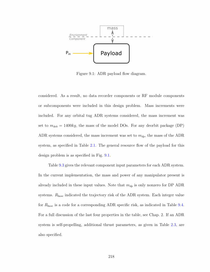
PayloadPin
Envrionment
Component
mass
Figure 9.1: ADR payload flow diagram.
considered. As a result, no data recorder components or RF module components
or subcomponents were included in this design problem. Mass increments were
included. For any orbital tug ADR systems considered, the mass increment was
set to mdeb = 1400kg, the mass of the model DOs. For any deorbit package (DP)
ADR systems considered, the mass increment was set to mdp, the mass of the ADR
system, as specified in Table 2.1. The general resource flow of the payload for this
design problem is as specified in Fig. 9.1.
Table 9.3 gives the relevant component input parameters for each ADR system.
In the current implementation, the mass and power of any manipulator present is
already included in these input values. Note that mdp is only nonzero for DP ADR
systems. Rbase indicated the trajectory risk of the ADR system. Each integer value
for Rbase is a code for a corresponding ADR specific risk, as indicated in Table 9.4.
For a full discussion of the last four properties in the table, see Chap. 2. If an ADR
system is self-propelling, additional thrust parameters, as given in Table 2.3, are
also specified.
218
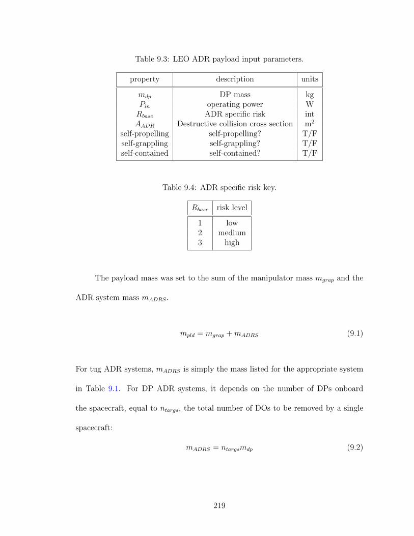
Table 9.3: LEO ADR payload input parameters.
property description units
mdp DP mass kgPin operating power WRbase ADR specific risk intAADR Destructive collision cross section m2
self-propelling self-propelling? T/Fself-grappling self-grappling? T/Fself-contained self-contained? T/F
Table 9.4: ADR specific risk key.
Rbase risk level
1 low2 medium3 high
The payload mass was set to the sum of the manipulator mass mgrap and the
ADR system mass mADRS.
mpld = mgrap +mADRS (9.1)
For tug ADR systems, mADRS is simply the mass listed for the appropriate system
in Table 9.1. For DP ADR systems, it depends on the number of DPs onboard
the spacecraft, equal to ntargs, the total number of DOs to be removed by a single
spacecraft:
mADRS = ntargsmdp (9.2)
219

For this design problem, the mass increment is managed by the payload. That
is, it is the payload that exchanges mass with the environment. For tug ADR
systems, the mass increment is set to 1400 kg, the mass of a DO. For DPs, it is
set to the mass of a single DP. This is because those are the increments by which
the spacecraft mass changes for the respective mission types. A tug grapples a DO,
increasing its mass by that of the DO. It then performs a series of maneuvers to
place the DO on a disposal orbit, subsequently releasing it, decreasing the spacecraft
mass by the mass of the DO. Conversely, an orbital tender vehicle performs plane
change between each DO, attaching an onboard DP to it. In doing so, it decreases
the spacecraft mass by the mass of a DP with each DO it visits.
9.3 GESDA Setup
As with the previous satellite design case, the CR flow diagram, given in
Fig. 9.2, is somewhat simplified from the generalized spacecraft topology. In this
case, thrusters and propellant tanks are present, as this is an active spacecraft
problem. However, RF modules, their subcomponents, and data recorders (those
component classes that deal only with data) are not. Data and telemetry from the
generalized spacecraft topology are omitted as resources.
9.3.1 L1 Genome
The L1 genome for this design problem contains six genes, which will be desig-
nated here L1i for the ith L1 gene. They are all drawn from the genome from Chap. 2,
220

Envrionment
Power
Generation
Power
Storage
Thruster
Payload
Propellant
Tank
ele
ctric
al p
ow
er
propellant
Spacecraft
thrust
solar flux
mass
Figure 9.2: CR flow diagram for the ADR vehicle.
221

capturing aspects of the design that are not accounted for in other portions of the
genome. L11 is ntargs, the number of DOs removed by each ADR vehicle. Accord-
ingly, it can have any integer value between 1 and 55, matching the conditions from
Chap. 2. L12 is a binary parameter, designating whether the spacecraft performs
impulsive maneuvers, or if maneuvers are considered low thrust. This is required for
any active spacecraft design problem, particularly those where the spacecraft ma-
neuvers in the simulation, as discussed in section 7.3.2. L13, L14, and L15 are binary
genes, indicating whether thrusters or payloads perform each maneuver type (orbit
raising, plane change, and orbit lowering, respectively). If the ADR system cannot
maneuver, these genes are ignored, and all maneuvers are performed by thrusters.
Finally, L16 is a binary gene that designates whether or not an ADR vehicle holds
short of high priority orbits, as discussed in Chap. 2.
9.3.2 Environment
The same model debris orbit outlined in Chap. 2 was used for this design prob-
lem. As this is a dynamic satellite design problem, with a maneuvering spacecraft,
the orbit simulation was procedurally generated. The orbital elements used are
given in Table 9.5. For this design problem, a heavily simplified orbital simulation
Table 9.5: LEO ADR orbital parameters, based on in Chap. 2.
a (km) e i (deg)
7128 0 74
was performed. The elements ω, ν, and Ω were not explicitly tracked, although ∆Ω,
222

the change in Ω between each DO orbit, as defined in Chap. 2, was. No simula-
tion was performed in GMAT or STK. Instead, a low fidelity simulation, with only
two timesteps per orbit, was performed. Matching the conditions of the original
LEO ADR work, direct sunlight was assumed for half of each orbit, constituting
one timestep, and complete darkness was assumed for the other half of each orbit,
constituting another timestep. Given the semimajor axis of the orbit, the orbital
period is 5989 seconds, or 1.66 hours. The duration ∆t of each timestep was there-
fore set to 2995 seconds. These two-timestep orbits were procedurally added to the
simulation, as dictated by section 7.3.2.
This decrease in fidelity was necessary to achieve reasonable runtimes. There
was never a plan to consider data downlink from the spacecraft for this design
problem. However, doing so would not even be possible with the current level of
reduced fidelity. See the final chapter of this dissertation for thoughts on addressing
this, should this work be extended in the future.
9.3.2.1 LEO ADR Maneuvers
This section details the logic behind the maneuver tables used for this design
problem. The formulation of each ∆V given here was taken directly from the original
LEO ADR work of Chap. 2. It is acknowledged that more accurate and efficient
formulations exist, especially for nonimpulsive maneuvers. However, effort was made
to accurately replicate the maneuver assumptions of the original LEO ADR work
to allow for a fair comparison of the results. Therefore, the work presented here is
223

really a more in-depth derivation of the maneuvers used for the original LEO ADR
work, which were preserved for the work of this chapter.
The ∆V tables for this mission take different forms depending on whether
the payload is a tug or orbital tender vehicle. For an orbital tender vehicle, the
spacecraft is assumed to be launched directly into the orbit of its first DO. The
∆V , therefore, only contains plane change maneuvers between each DO. As in the
original LEO ADR study, nodal regression is not considered, so it is assumed that
all plane change between DOs must be accomplished propulsively. As a result, each
line of the ∆V table is identical, taking the form given in Table 9.6. where ∆VΩ is
Table 9.6: ∆V table format for orbital tender vehicles.
∆V (m/s) twait (orbits) mass increment thruster class maneuver type
∆VΩ 48 -1 L14 plane change
the plane change ∆V , the form of which depends on multiple L1 genes, as discussed
below. A 48 orbit ( 3 day) wait after the completion of each maneuver is included, as
was the case in the original LEO ADR study, to account for phasing and rendezvous
with the next DO. The mass increment of -1 accounts for the loss of mass as each DP
is removed from the spacecraft and attached to the DO. As discussed above, L14
indicates whether the ADR system or thrusters perform plane change maneuvers
(the only maneuver type conducted for orbital tender vehicles). Note, however, that
no DPs considered are self-propelling, so in this design study, all maneuvers for
tender vehicles, including plane change maneuvers, were performed by thrusters.
224

The form of ∆VΩ depends on ntargs, the number of DOs removed per ADR
vehicle, and on whether or not the ADR vehicle performs impulsive maneuvers.
Both are specified by L1 genes. ntargs determines ∆Ω. Taking the distribution in
Ω of the model DO population, the total plane change Ωtot,min of the most tightly
bound group of ntargs DOs in the population is found. ∆Ω is then
∆Ω =Ωtot,min
ntargs, (9.3)
the average plane change between successive DOs. ∆VΩ is then a function of ∆Ω,
with its form depending on whether or not maneuvers are impulsive. For impulsive
maneuvers,
∆VΩ = 2
õ
asin
(∆Ω
2
)(9.4)
Nonimpulsive maneuvers were adapted from the work of Stansbury [77], which
was in turn adapted from [78]. The initial yaw angle β0 is first found from Eq. 14.38
in [78]:
β0 = tan−1
(sin(π2∆Ω)
V 0Vf− cos
(π2∆Ω)) (9.5)
Where V0 is the spacecraft velocity on the initial circular orbit, and Vf the velocity
on the final circular orbit. For orbital tender vehicles, the orbital altitude does not
change, so V0 = Vf . With β0, the total ∆V for the plane change maneuver is, as
given in Eq. 14.73 in [78]:
∆VΩ = V0
(cos β0 −
sin β0
tan(π2∆Ω + β0
)) (9.6)
225

Due to nodal regression, this is considered a worst case ∆V . Finally, then, the ∆V
table for orbital tender vehicles is ntargs repetitions of Table 9.6.
For orbital tugs, the form of the maneuver table depends on whether or not
maneuvers are impulsive, as well as whether or not the same thruster class is used
for each maneuver type. If maneuvers are not impulsive, and the thruster class is
the same for orbit raising and plane change maneuvers, these two maneuvers can be
combined. Eqs. 9.5 and 9.6 can be used to calculate ∆Vc, the combined ∆V to raise
the orbit and perform the necessary plane change. In this case, V0 is the velocity of
a 200 km circular orbit (the debris disposal orbit, which is also the orbit into which
nonimpulsive orbital tugs are initially launched), and V1 is the velocity in the debris
orbit. If maneuvers are not impulsive and orbit raising and plane change cannot be
combined, then the ∆VΩ is computed with Eq. 9.6, and ∆Vup, the ∆V required for
plane change, is assumed to be the difference of the velocities of the two circular
orbits:
∆Vup = V0 − V1 (9.7)
Since the nonimpulsive tug is always maneuvering between two set orbital altitudes,
the debris altitude of 750 km, and the disposal altitude of 200 km, orbit raising and
lowering maneuvers are of the same magnitude (though the total impulse is not,
given the additional DO mass on the way down). Therefore,
∆Vdown = ∆Vup (9.8)
226

For impulsive maneuvers, orbit raising and plane change are not combined.
The ADR vehicle is assumed to start in a 750 km × 200 km orbit. For orbit raising,
the vehicle circularizes itself at apogee into the debris orbit. It then performs any
necessary plane change, rendezvouses with and captures the DO. For lowering the
DO, a Hohmann transfer is performed, lowering the debris perigee to 200 km as
specified in Chap. 2. Again, due to the symmetry of orbit raising and orbit lowering,
both require the same ∆V :
∆Vup = ∆Vdown = 175 m/s (9.9)
Impulsive plane change is performed in the same manner as for tender vehicles, and
is therefore given by Eq. 9.4, with a being the semimajor axis of the debris orbit.
For impulsive maneuvers, and nonimpulsive maneuvers where plane change
and orbit raising are not combined, the ∆V table starts with the initial orbit raising
after launch, and the subsequent orbit lowering after capturing the first DO, as
shown in Table 9.7 For all remaining maneuvers a block of the form given in Table 9.8
Table 9.7: Initial ∆V table for orbital tugs.
∆V (m/s) twait (orbits) mass increment thruster class maneuver type
∆Vup 1 1 L13 orbit raising∆Vdown 1 -1 L15 orbit lowering
is appended to the ∆V table ntargs − 1 times, to account for all DOs removed after
the first.
227
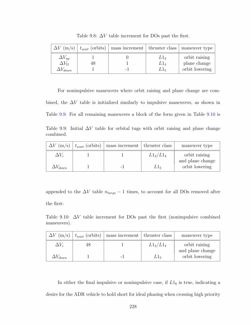
Table 9.8: ∆V table increment for DOs past the first.
∆V (m/s) twait (orbits) mass increment thruster class maneuver type
∆Vup 1 0 L13 orbit raising∆VΩ 48 1 L14 plane change
∆Vdown 1 -1 L15 orbit lowering
For nonimpulsive maneuvers where orbit raising and plane change are com-
bined, the ∆V table is initialized similarly to impulsive maneuvers, as shown in
Table 9.9: For all remaining maneuvers a block of the form given in Table 9.10 is
Table 9.9: Initial ∆V table for orbital tugs with orbit raising and plane changecombined.
∆V (m/s) twait (orbits) mass increment thruster class maneuver type
∆Vc 1 1 L13/L14 orbit raisingand plane change
∆Vdown 1 -1 L15 orbit lowering
appended to the ∆V table ntargs − 1 times, to account for all DOs removed after
the first:
Table 9.10: ∆V table increment for DOs past the first (nonimpulsive combinedmaneuvers).
∆V (m/s) twait (orbits) mass increment thruster class maneuver type
∆Vc 48 1 L13/L14 orbit raisingand plane change
∆Vdown 1 -1 L15 orbit lowering
In either the final impulsive or nonimpulsive case, if L16 is true, indicating a
desire for the ADR vehicle to hold short for ideal phasing when crossing high priority
228
orbits, a pause duration of one orbit was added to each orbit lowering maneuver in
the ∆V table.
9.3.2.2 Propulsive Multistep
Based on the procedural nature of the simulation, low thrust maneuvers that
take many orbits to perform necessitate very large simulation files, with 2No timesteps,
where No is the number of orbits in the simulation. For low thrust propulsion sys-
tems, which including all electric propulsion thrusters considered, as well as the LAT
and EDDE payloads, No can be on the order of 100ntargs or greater. As a result, for
practical computational reasons, it was necessary to reduce the number of timesteps
actually simulated. This was accomplished with a special propulsive multistep. The
propulsive multistep is, in most ways, identical to the regular multistep, discussed
in section 7.3.2. While the regular multistep is only performed once a maneuver
has been completed, a propulsive multistep is performed if more than ten timesteps
are required to complete the current maneuver. The propulsive multistep, operates
under the implicit assumption that any low thrust propulsion systems do not sig-
nificantly change the mass of the spacecraft over a single maneuver. This proved to
provide comparable results for this design problem, but may not be applicable in
general.
If used, the propulsive multistep simulates a single orbit and performs a regular
multistep internally with a number of repetitions
r = floor(∆Vi/∆Vp), (9.10)
229

where ∆Vi is the ∆V remaining in the current maneuver, and ∆Vp is the ∆V
performed over a single orbit. It then additionally calculates the total ∆V performed
over the multistep
∆Vtot = r∆Vp (9.11)
and subtracts this from the ∆V remaining in the current maneuver.
9.3.3 Components Used
The components used in this design problem correspond to the original mod-
eled subsystems from Chap. 2. This comprises PVAs, batteries, thrusters, and pro-
pellant tanks from the general CR model for spacecraft design, as shown in Fig. 7.1,
as well as payloads, as detailed in this chapter. For propellant tanks, a separate class
was specified for each type of propellant included, as discussed in Chap. 7. A single
list of tanks was used to populate the component library for all liquid propellant
tank classes. A separate list was used to populate the component library for gaseous
tank classes, of which Xenon was the only one in this design problem. Addition-
ally, collision avoidance motors were included as a component class. They are not
included in Fig. 9.2, as they do not feature any resource flow. For the purposes of
the simulation, they are an additional inert mass, which influences the overall risk
factor, modifying the objective functions as discussed in Chap. 2. For a complete
list of components used for this design problem, see Appendix C.
For optimization, a constraint of one payload per spacecraft was added as a
component quantity constraint. All other component quantities were unconstrained,
230

but seed ranges were specified for each class. These are used when initializing the
first generation of designs, but do not constrain the number of components in each
class in any later generations. The seed ranges for each unconstrained class are
given in Table 9.11.
Table 9.11: Seed ranges for unconstrained component classes.
class name minimum quantity maximum quantity
PVAs 0 10batteries 0 10thrusters 1 10
collision avoidance motors 0 55MMH tanks 1 10NTO tanks 1 10
Aerozine 50 tanks 1 10N2H4 tanks 1 10Xenon tank 1 10
9.3.4 Objective Functions
The objectives for this design problem were to minimize cDO, the cost per DO
removed, and to minimize the overall risk factor ORF . The total spacecraft mass
mtot, and, subsequently, cDO, which is a function of mtot were defined as discussed
in section 2.2.3.1. ORF was defined by Eq. 2.5.
9.4 Results and Comparison to Original LEO ADR Study
The baseline scenario from the original LEO ADR study was replicated with
GESDA, as outlined in this chapter. Separate runs of GESDA were performed for
231
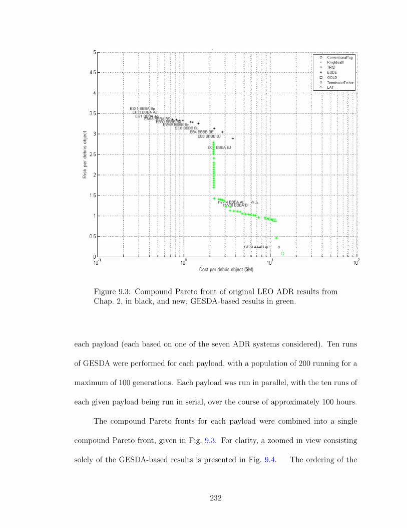
Figure 9.3: Compound Pareto front of original LEO ADR results fromChap. 2, in black, and new, GESDA-based results in green.
each payload (each based on one of the seven ADR systems considered). Ten runs
of GESDA were performed for each payload, with a population of 200 running for a
maximum of 100 generations. Each payload was run in parallel, with the ten runs of
each given payload being run in serial, over the course of approximately 100 hours.
The compound Pareto fronts for each payload were combined into a single
compound Pareto front, given in Fig. 9.3. For clarity, a zoomed in view consisting
solely of the GESDA-based results is presented in Fig. 9.4. The ordering of the
232

100
101
0
0.5
1
1.5
2
2.5
3
Cost per debris object ($M)
Ris
k pe
r de
bris
obj
ect
Compound Pareto Front
Figure 9.4: GESDA-based compound Pareto front of LEO ADR vehicles.
233

designs, and their share of the Pareto front, is relatively unchanged from the original
LEO ADR work. The majority of the front is EDDE-based designs, which represent
the highest risk/lowest cost. In the middle of the front are a relatively small number
of LAT-based designs, followed by a single other design, either a conventional tug
in the new results or Terminator Tether in the original results.
At first glance, the results appear complementary - filling in different portions
of the same Pareto front. This is more or less true for three points on the lower right
edge of the Pareto front. However, the middle “flat” portion of the new Pareto front,
from a cost per DO of $2M to $11M, consists of similar designs to the remainder
of the original Pareto front. Comparable designs on the new front are somewhat
more expensive, while at the same time substantially lower risk than their original
counterparts.
This is, regrettably, due to a bug found in the original risk calculation code,
which inaccurately modified the weighted technology readiness level (WTRL) all
orbital tug designs. Specifically, the error forces all orbital tug payloads to TRL
2. In the original LEO ADR work, all EDDE designs were self-contained. These
designs contained no components other than the EDDE payload itself, and possibly
collision avoidance motors, whose mass was insignificant to EDDE. As a result the
WTRL of those spacecraft was 2 or very close to 2, compared to the WTRL of
5 it should have been. Given Eq. 2.3, this produces an RSS of 2.7 for WTRL 2
compared to 0.5 for TRL 5. Given [42], a WTRL of 5 produces a value of 1.3 for
fC , as opposed to 3 for a WTRL of 2. Since EDDE was the only self-contained
ADR system, it was dramatically impacted by this error, while the Pareto-optimal
234

Figure 9.5: Corrected compound Pareto front.
designs utilizing other payloads were not. Fig. 9.5 presents the same data as Fig. 9.3,
shifting the self-contained EDDE designs to correct for this error. As can be seen,
this brings ORF values for EDDE into line with the corresponding portions of the
new Pareto front.
Investigating the lowest risk LAT from both the original and new study, the
risk is approximately 1.0 in the GESDA-based results, whereas it was originally 1.3.
The number of DOs removed per spacecraft, as well as the respective components of
ORF for these two designs is given in Table 9.12. where TPO is the time per object
per ADR vehicle. Note this does not necessarily directly result from ntargs and the
requisite 100 total DOs removed. TPO also takes into account the requirement that
10 DOs be removed per year, and given the average time per DO removed per ADR
vehicle, increases the fleet size as necessary.
235

Table 9.12: Parameter comparison for old and new LEO ADR LAT results.
parameter original value GESDA value
mtot (kg) 487 475TPO (days) 357 662ntargs 14 6NF 10 19
WTRL 5.0 7.99RT 0.90 0.83RTRL 0.44 0.14
At a glance, the two spacecraft are physically fairly similar. Both have the
same payload and very similar mtot. The difference in ntargs directly leads to the dif-
ference in fleet size NF required to remove the 100 objects specified for the program.
This difference in NF entirely accounts for the difference in RT . The difference in
RTRL results from a difference in how WTRL is calculated between the old design
optimizer and GESDA. Originally, due to the limited knowledge of individual space-
craft components, WTRL was calculated as discussed in section 2.2.3.2. In GESDA,
where the individual TRL of each component is tracked, it is possible to calculate
WTRL on a component-by-component basis:
WTRL =∑
spacecraft
mdry,i
mdry
TRLi (9.12)
where mdry,i is the dry mass of component i, TRLi is the TRL of component i,
and mdry is the dry mass of the entire spacecraft. As opposed to in [43] where
WTRL was weighted by the cost of each component, it is instead weighted here by
component mass, which is used as a rough stand in for cost, since component costs
236

were not available. As was the case for EDDE, this difference in WTRL entirely
accounts for the change in RTRL.
Perhaps the two most striking differences in the Pareto front are the presence
of an EDDE-based design in the lower right portion of the front, and the nearly
vertical column of low cost EDDE-based designs comprising the leftmost portion of
the front. The single “low risk EDDE” design is a self contained EDDE spacecraft
that only removes a single debris object. In doing so, it completely eliminates its
trajectory risk, but substantially increases program cost, with a separate vehicle now
required for each DO. It is likely that a similar design could have been present in the
original results, but due to the TRL error for EDDE, would have been dominated
by other designs, and therefore not appear on the Pareto front.
All designs in the near vertical column on the far left are EDDE-based, and
have 27 ≤ ntargs ≤ 29. The difference between the designs in this “tail” is the
number of collision avoidance motors attached. Based on Eq. 2.1, holding all other
variables constant, each addition or removal of a collision avoidance motor causes a
constant change in RT . The addition of the mass of each motor slightly increases
the spacecraft mass. As one travels up the tail, removing motors, the mass of the
spacecraft decreases accordingly. If the spacecraft is otherwise identical, this will
lead to a slight decrease in the cost per DO removed. An exhaustive exploration
of the design space would produce similar tails, rising vertically from each Pareto-
optimal design for which RM > 0. However, all other tails will be dominated by the
tail of lower cost designs, except for the lowest cost design, so they do not appear
on the Pareto front.
237
It is suspected that no such tails appeared in the original LEO ADR design
study due to use of single fitness function given by Eq. 2.6. This did produce a single
fitness value for the multiple objectives, but likely introduced a bias towards lower
risk, producing a more even spread across cost, but not fully capturing the Pareto
front. Conversely, a form of NSGA-II [23], which by design favors even spread across
the Pareto front, was used for GESDA.
An additional notable change is that the conventional tug is on the Pareto
front, taking the approximate place of Terminator Tether from the original study.
Though the conventional tug was not on the Pareto front in the original study, it
was observed to be close to it. It is likely that the correction of the TRL bug for
orbital tugs, discussed above, lowered the risk of the conventional tug, improving its
performance. The performance of Terminator Tether is comparable to the conven-
tional tug throughout, with both achieving an ORF of 0.0755, and with Terminator
Tether achieving a cost of $19.7M per DO. It is possible, though considered unlikely
with ten trials of each payload, that random chance associated with use of a GA
determines which of these two systems dominates the other.
One observation that is clear from Fig. 9.5 is a substantial increase in cost per
DO across the Pareto front. Consider again the LATs investigated in Table 9.12.
Their cost breakdown is given in Table 9.13. The majority of these costs are fairly
comparable, with the exception of the bus development and first unit production
costs, and in particular the total production cost. The bus-related costs were ap-
proximately 50% higher cost than in the original study. The differences in the bus
of the two designs, leading to this discrepancy, will be discussed below. The total
238

Table 9.13: Cost comparison for old and new LEO ADR LAT results, with all costsin $M.
cost category original value GESDA value
ADR system development cost 34.1 38.9Bus development cost 86.8 128ADR system first unit cost 10.7 12.6Bus first unit cost 17.8 28.5
Total production cost 191 451Launch cost 22.6 22.5
Cost per DO removed 6.2 11.6
production cost is 2.4 times as great than in the original study. Due to the sub-
stantial difference in ntargs (the difference in TPO also plays a role, but ntargs is the
dominant factor), nearly double the fleet size is required to remove the requisite 100
DOs.
The difference in cost per DO between the old and new results is even more
pronounced for EDDE. Compare the GESDA-based EDDE design in the lower left
corner of the Pareto front (the one at the “head” of the vertical tail on the left), and
the second EDDE design from the left in the original ADR study. These two are
chosen for comparison as they have similar values for ntargs. A comparison of their
parameters is given in Table 9.14. As can be seen, the risk factors are essentially
identical. All parameters in the table are essentially the same, with the exception
of TPO. Upon further investigation of the original LEO ADR work, the original
value used for the maneuvering performance of EDDE conflicts with the source
used for the GESDA-based design study, both from the same author, who is the
PI for EDDE. However, the time per DO removed was not an active constraint, as
239

Table 9.14: Parameter comparison for old and new LEO ADR EDDE results.
parameter original value GESDA value
mtot (kg) 85 80TPO (days) 32 116ntargs 32 29NF 4 4
WTRL 5 5RT 0.96 0.96RTRL 0.45 0.46
noted by the fact that NF is the same for both, and therefore this discrepancy is
not considered to have a substantial effect on the design space.
Table 9.15 gives the cost breakdown for the same two designs. Note that,
unlike for the LAT example above, both EDDE vehicles were assumed totally self-
contained in the original study. Therefore, development and production costs were
not separated by bus and payload. In the work of this chapter, a lump mass 7/3 of
Table 9.15: Cost comparison for old and new LEO ADR EDDE results, with allcosts in $M.
cost category original value GESDA value
ADR system development cost 22.5 22.5Bus development cost - 62.8ADR system first unit cost 7.68 7.68Bus first unit cost - 12.1
Total production cost 25 64.1Launch cost 3 3
Cost per DO removed 0.815 2.25
the mass of the ADR system is added for EDDE (as it is for all non-self spacecraft) to
account for unmodeled masses, such as structural mass, communications subsystems,
240

and attitude control. As a result, there are nonzero bus development and production
costs, resulting in the threefold increase in EDDE production costs seen in the new
results compared to the original ones. Since, even with this threefold increase,
EDDE still comprises the upper left portion of the Pareto front, this discrepancy
does not change the relative ordering of results on the Pareto front. Nonetheless,
more thought may be warranted on what the proper treatment of EDDE compared
to the other designs on the Pareto front. It is in many ways an unconventional
spacecraft, and special considerations in the objective functions may be warranted
to handle this. However, these considerations must be weighed against the loss
of generality, and unintended consequences for introducing a different treatment of
ADR systems under consideration.
This concludes the comparison of the LEO ADR vehicles designed here to
those from Chap. 2. The remainder of this section provides a comparison of designs
from the different “families” on the Pareto front. This is done in the same spirit
as, for example, Table 2.8, though the differentiation between families of designs
is far less pronounced than in the original study. This is suspected to be due to
the use of an NSGA-II derived sorting algorithm, which performs more complete,
continuous exploration along the Pareto front than the original fitness function used
in Chap. 2. Even so, the designs can still be grouped by payload, with each payload
occupying a particular portion of the Pareto front. Table 9.16 provides high-level
details on the lowest cost per DO design of each family on the Pareto front. An
exception is made for EDDE, where the lowest cost per DO design would be the
end of the tail, which has nearly the same cost per DO as the “head” of the tail,
241
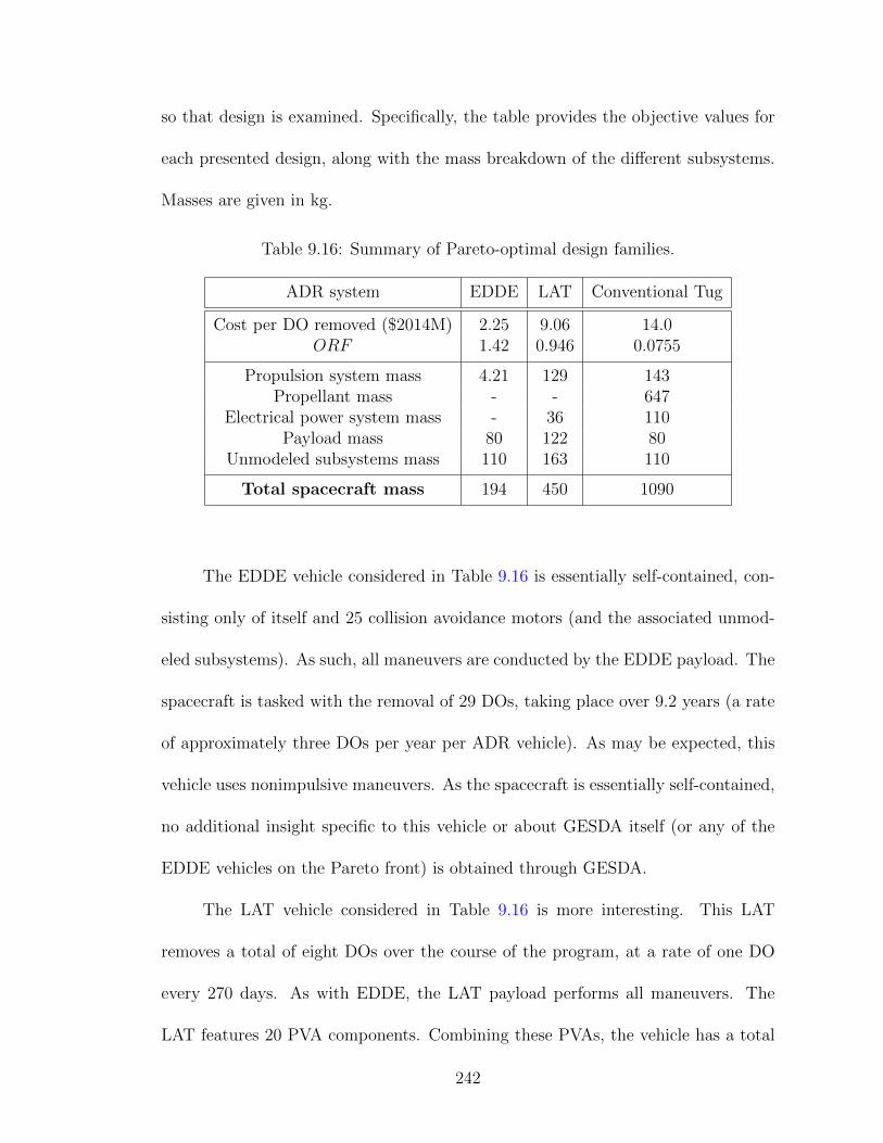
so that design is examined. Specifically, the table provides the objective values for
each presented design, along with the mass breakdown of the different subsystems.
Masses are given in kg.
Table 9.16: Summary of Pareto-optimal design families.
ADR system EDDE LAT Conventional Tug
Cost per DO removed ($2014M) 2.25 9.06 14.0ORF 1.42 0.946 0.0755
Propulsion system mass 4.21 129 143Propellant mass - - 647
Electrical power system mass - 36 110Payload mass 80 122 80
Unmodeled subsystems mass 110 163 110
Total spacecraft mass 194 450 1090
The EDDE vehicle considered in Table 9.16 is essentially self-contained, con-
sisting only of itself and 25 collision avoidance motors (and the associated unmod-
eled subsystems). As such, all maneuvers are conducted by the EDDE payload. The
spacecraft is tasked with the removal of 29 DOs, taking place over 9.2 years (a rate
of approximately three DOs per year per ADR vehicle). As may be expected, this
vehicle uses nonimpulsive maneuvers. As the spacecraft is essentially self-contained,
no additional insight specific to this vehicle or about GESDA itself (or any of the
EDDE vehicles on the Pareto front) is obtained through GESDA.
The LAT vehicle considered in Table 9.16 is more interesting. This LAT
removes a total of eight DOs over the course of the program, at a rate of one DO
every 270 days. As with EDDE, the LAT payload performs all maneuvers. The
LAT features 20 PVA components. Combining these PVAs, the vehicle has a total
242

solar array area of 145 m2, producing a total of 5.8 kW of power. This is far more
than the 250 W required to power the spacecraft at any given time. Understanding
the nature of this discrepancy requires a brief discussion of the state of the GESDA
component libraries.
The PVA component library for this design problem included a number of
simulated components. Data was only available for individual solar cells and small
arrays, with component suppliers indicating that panels are built to order depending
on the requirements at hand. Since GESDA relies on fixed components to operate, a
workaround was implemented to add “macrocomponents” that were the equivalent
of 3, 10, 30, 100, 300, and 1000 copies of the XTJ 5965 solar panel by Spectrolab,
combined into a single panel. The goal of adding these components of varying sizes
is to allow GESDA to build up large enough components to achieve feasibility in a
small number of generations.
Of the 58.4 kW of power produced by the spacecraft while in sunlight, 48 kW
resulted from two of the largest of these macrocomponents, the “1000x XTJ 5965,”
and an additional 9.6 kW resulted from four of the “100x XTJ 5965” macrocom-
ponents. Each of the 1000x XTJ 5965 panels had a mass of approximately 5 kg,
and each 100x XTJ 5965 panel had a mass of approximately 0.5 kg. This leaves 800
W of electrical power coming from the remaining solar arrays. Assuming perfectly
efficient batteries, 500 W is required from the PVAs when in sunlight to power the
spacecraft. Therefore, all of these panels are unnecessary for feasibility. However,
their combined mass is only 12 kg, comprising less than 3% of the total spacecraft
mass. Removing these components from the design and re-running the objective
243
functions, one finds that their removal has only reduced the cost per DO removed
from $9.06M to $8.96M, a change of approximately 1.1%. This is definitely a real
effect, but the change in objective performance of the overall design is not signifi-
cant. Additionally, it does not affect the relative performance of the different designs
present on the Pareto front.
Throughout analysis of the GESDA results, multiple cases of such “vestigial
components” (to borrow a term from biological evolution) were present. That is,
additional components that may have been required for feasibility or had a signifi-
cant effect on performance of some ancestor of the final design. Through the GA,
these components were inherited, but are not required for the feasibility of perfor-
mance of final design itself. They do not adversely affect the overall performance
of the final design, so they persist. Additional generations of the GA may even-
tually lead to their removal. However, if the design space has converged, this is
not necessarily computationally efficient. If the design space has been sufficiently
explored, such “trimming” may not be necessary. Perhaps a better option is, at
this point, to transfer some set of Pareto-optimal designs to a human designer or
concurrent design team, who would perform any final trimming before or as part of
their concurrent design campaign.
A single battery is present in this LAT design, drawn from the Soil Moisture
Active Passive (SMAP) spacecraft. Four thrusters are present, all assumed vestigial,
since no propellant tanks are present, and all maneuvers, based on the L1 genome,
are performed by the LAT payload. Thirteen collision avoidance motors are present.
Removing the vestigial thrusters and PVAs lowers the mass of the spacecraft to 311
244

kg and lowers the cost per DO removed to $7.9M. Interestingly, it does slightly
increase the ORF to 1.01. This is a result of removing components whose TRL was
actually above the WTRL of the spacecraft. Since, by Eq. 9.12, WTRL is weighted
by mass, their removal lowers the WTRL of the spacecraft from 8 to 7, leading to
this slight increase in risk. Interestingly, this slight increase in risk means that the
design is now dominated by an EDDE-based design on the Pareto front, though the
objective performance of this design is still extremely close to the Pareto front.
Finally, we arrive at the conventional tug on the Pareto front. It only removes
four DOs per vehicle, limited by the propellant it must carry to reach each DO.
Each ADR vehicle performs impulsive maneuvers, and as a result removes a DO
approximately once every three days, deorbiting itself with the last DO at the end
of a two week mission. As was the case in the original work of Chap. 2, the impulsive
conventional tug minimized RT , maneuvering each DO directly from their original
orbit onto a targeted reentry trajectory. Due to the large amount of propellant
required for impulsive thrusters, the spacecraft mass is large compared to the other
designs on the Pareto front.
Investigating the electrical power subsystem for the conventional tug, a similar
situation appears to that of the LAT, with PVAs producing a total of 29.0 kW of
power. Indeed, investigation of the component structure reveals that the majority
of the electrical power (23.9 kW) comes from a single vestigial 1000x XTJ 5965.
The design also contains a number of vestigial thrusters. An investigation of the fill
levels of onboard propellant tanks reveals that only a single R-4D thruster is used
to perform all maneuvers. The design features two batteries, with a total capacity
245

of 756 W-h (one a 504 W-h battery, and one a 252 W-h battery). With an orbital
night duration of approximately 50 minutes, and a power draw of 131 W during
orbit night, this leads to a 14% depth of discharge. Therefore, both batteries are
required to meet spacecraft requirements.
Removing the vestigial thrusters, propellant tanks, and PVAs, a slightly lighter
spacecraft at 1015 kg is achieved. The cost per DO has decreased accordingly, to
$13.8M, an approximately 1.5% decrease. The ORF of the spacecraft is unchanged.
Again we see that the removal of vestigial components causes a marginal improve-
ment, but does not significantly affect the objective performance of the design.
9.5 Summary
In this chapter we have demonstrated the use of GESDA for active spacecraft
trade space exploration. The chapter has readdressed the design problem originally
addressed in Chap. 2, active debris removal in Low Earth Orbit. In doing so, it
provides an additional level of detail over the original study, simulating the ADR
vehicle designs to a component level. The results of this chapter, while producing
different numerical results, have essentially confirmed the conclusions of the primary
trade study performed in Chap. 2, for the nominal scenario of that chapter. While
the overall conclusions are the same, there are some notable differences. The highest
cost per DO removed, lowest risk designs on the Pareto front have changed, with
the single orbital tender vehicle being traded for a impulsive conventional tug.
246

The overall conclusions are very similar to those of Chap. 2. This agreement
acts to verify the performance of GESDA for trade space exploration with active
spacecraft missions. One can see that propellantless tugs dominate the Pareto front,
and orbital tender vehicles are not present. The performance of propellantless tugs
is, as before, due to the decoupling of their mass from the number of DOs they
remove (though, to maintain the requisite removal rate, there is still an implicit
relation between the two). Their resulting ability to deorbit a relatively large number
of DOs with a single vehicle drives down the cost per DO. As before, this does carry
the drawback of higher risk. The propellantless tugs considered have relatively
limited maneuvering ability, so they must spiral down to a disposal orbit, detach
the DO, and then spiral back up to the next DO. The disposal orbit altitude is
limited to one where their limited maneuvering ability is still able to overcome
atmospheric drag. As a result, the reentry of the DOs from this disposal orbit is
guaranteed in a relatively short timeframe, but still long enough that the impact
location is unknown.
As was originally the case, no electric propulsion systems are present in any of
the designs on the Pareto front (not counting the payloads of the LAT and EDDE,
which could be construed as electric propulsion systems). Investigation of dominated
designs in the original study which did use electric propulsion suggests that the time
per DO removed using these systems is too great to be feasible with a reasonable
fleet size.
The key difference from the results of Chap. 2 is that conventional tugs have
replaced Terminator Tether on the Pareto front. During the original LEO ADR
247

study, Terminator Tether-based designs and impulsive conventional tugs continu-
ally traded places on the Pareto front, each dominating the other in some cases.
Their performance was so similar that, as indicated in Chap. 2, both were consid-
ered worthy of further study. The impulsive conventional tugs in particular are the
minimum risk system on the Pareto front, but are only able to deorbit a small num-
ber of DOs per vehicle before required propellant makes their mass prohibitive. The
one considered here, for example, deorbits after only removing 4 DOs. This small
ntargs for conventional tugs makes one consider if they may be able to perform at a
much reduced cost per DO removed if they were somehow reusable, able to conduct
multiple 4 DO missions. Potential options include reusable spacecraft somehow ca-
pable of controlled reentry and landing, or the use of orbital fuel depots to allow
the conventional tug to refuel between DOs.
248
Chapter 10: Conclusions and Final Thoughts for Derived Works
At this point, this work, at least in the context of a PhD study, is consid-
ered complete. The orbital debris problem has been addressed with two different
methods, producing similar results for the lowest risk and lowest cost per DO re-
moved options. The CR model, applicable to a wide class of complex systems, has
been developed. An architecture has been constructed around it, allowing auto-
mated optimization routines to understand the general spacecraft design problem
from a high-level systems aspect. The framework has been applied to two space-
craft design problems, and has produced results within the range of flown vehicles
and other studies. The remainder of this chapter summarizes the conclusions of the
entire work, and provides some insight from the work performed to guide anyone
interested in conducting follow-on work.
10.1 Summary and Conclusions
This work initially started as an attempt to provide an objective comparison
of proposed systems for removing large, intact debris objects from low Earth orbit
(LEO). Several payloads have been proposed, and the goal was to develop a simu-
lated scenario that evaluates the performance of each. A framework was developed
249

that could take the mass, power, and maneuvering requirements properties of any
such active debris removal (ADR) payloads, design spacecraft around them, and
determine the risk and cost per object removed of each. The final results, which
would later be largely confirmed by the final form of this work, were fairly clear.
There is a clear financial advantage to the use of “propellantless” tugs, which need
not carry a set mass onboard for each debris object (DO) removed. However, doing
so, at least with currently available technology, does carry a substantially increased
risk. As a result of this risk, a low risk, more conventional spacecraft design always
accompanies these designs in the trade space.
Two propellantless systems were evaluated. The first was an electrodynamic
tether propelled orbital tug (EDDE), which captures DOs in a net and maneuvers
through interactions with Earth’s magnetic field. The second was a laser ablation
tug (LAT), which captures DOs with a robotic arm, and ablates material from
the DO to provide thrust, using the DO itself as propellant. In doing so, the
LAT is not propellantless in the truest sense of the word. In fact, in the case of
EDDE, the Earth itself could be considered the propellant, making neither system
propellantless. The key aspect is that these designs need not carry all propellant
mass for their mission from one DO to the next. Investigations into other concepts
which follow this same principle with more conventional spacecraft are suggested in
the recommended future work below.
The elevated risk of the propellantless systems stems from two sources. One
is their low technological maturity, calling into question when and if they would be
ready to enter service as the debris environment continues to worsen. The other risk
250

is associated with the fact that both propellantless systems considered are of such
low thrust that they cannot place DOs tugged onto a targeted reentry trajectory.
They must, with DO in tow, spiral down to a disposal orbit low enough that the DOs
will reenter in a relatively short timeframe, but high enough that, after releasing
the DO, the vehicle itself is capable of escaping the thin atmosphere to capture the
next DO.
The lower risk system appearing on the Pareto front was always a conventional
orbital tug, or a low risk orbital tender vehicle. The conventional orbital tug consists
of a robotic arm and conventional impulsive propulsion system for moving the DO
in orbit. It can be assembled entirely out of currently flight proven components,
with the exception of hardware for grappling an uncooperative DO, and associated
sensor systems. Both of these technologies are on track for flight validation in
the immediate future [79–81]. The other low risk system appearing on the Pareto
front is an orbital tender vehicle delivering Terminator Tether [31] to a number
of DOs. Terminator Tether was a package that could be attached to a DO, and
could extend or retract a drag tether to lower the DO’s orbit. Due to its ability to
retract, it was capable of targeted reentry, eliminating the biggest source of risk of
the propellantless tugs.
The key takeaway is that, from an engineering standpoint, active debris re-
moval in LEO is viable with current technologies. Depending on the level of risk
that society deems acceptable, this debris removal can be accomplished with current
technologies for approximately $10M, and with technologies under active develop-
ment for single millions of dollars. The work detailed in this section was originally
251

conducted from 2013 to 2016. Trends in the space industry since that time have
intensified the need for this sort of debris removal program. At the same time,
many of these same trends (the move towards smallsats and large constellations of
cubesats) will likely help facilitate such a program.
The work of Chapter 2, as well as associated small bodies mission and robotic
satellite servicing work being conducted simultaneously by the author, led to the
idea of creating a generalized framework that, with little to no modification, could
perform systems-level analysis of a wide range of space missions. This concept
motivated the remainder of the dissertation. Chapters 3 through 6 presented the
Component-Resource (CR) model and associated Vehicle Encoding Genetic Algo-
rithm (VEGA). The CR model presents a uniform method of analyzing any complex
system that comprises discrete components and resources flowing among them. It
facilitates feasibility analysis of such a system in a uniform way, based on the re-
source flows. VEGA then performs optimization of such systems, using the CR
model to evaluate constraints in a uniform way, facilitating optimization of a wide
range of complex systems.
Chapter 7 presented a VEGA-based Generalized Evolutionary Spacecraft De-
sign Architecture (GESDA) to perform spacecraft design optimization. GESDA
maintains the driving philosophy of generality, while acknowledging that certain
design problem-specific considerations are unavoidable. It attempts to present a
general framework that is at least capable of addressing a wide range of spacecraft
design problems. In doing so it separated spacecraft into two general categories;
passive and active spacecraft.
252
Passive spacecraft are assumed to be on a fixed orbit trajectory, and as such are
evaluated in a fixed simulation. They do not manipulate or physically interact with
their environment (that is, the environment is unaffected by what the spacecraft is
doing). This covers any mission types that could be analyzed with the GINA model
[22]. Active spacecraft can maneuver and manipulate portions of their environment.
As a result, they introduce additional complexity into the simulation, requiring a
lower fidelity simulation to maintain computational feasibility.
Finally, Chapters 8 and 9 presented active and passive use cases of GESDA,
respectively. Chapter 8 sought to evaluate designs for an Earth observing cubesat. It
did so by developing spacecraft to support the PlanetScope 2 (PS2) payload carried
by the Dove spacecraft produced by Planet Labs. In doing so it explored a relevant
trade space to the Dove spacecraft; the trade between spacecraft mass, assumed to
correlate with program cost, and imaging data returned. The results were a Pareto
front containing designs which came relatively close to the performance of the Dove
spacecraft (around 120% of the mass for the same data returned). Given the step
function-like nature of the Pareto front, it is likely that there are other trade spaces
of interest to this mission.
Some difference is acknowledged between the simulated mission profile imple-
mented in Chapter 8 and the actual Dove 3 mission profile. This is partially due
to simplifying assumptions made to streamline the simulation, and partially due to
the limited data available on the Dove mission design. Nonetheless, the results of
Chapter 8, which did come reasonably close to the actual Dove spacecraft design,
are considered informative in selecting a spacecraft design for further evaluation.
253

Interestingly, the “agile aerospace” design philosophy behind the Dove space-
craft is simultaneously very similar to and at odds with the design philosophy as-
sumed by this work. It rejects the aerospace industry convention of detailed con-
current design of monolithic, high reliability, risk averse spacecraft comprising all or
nearly all flight proven, space grade hardware. Instead, Planet operates with a large
quantity of small, expendable spacecraft with terrestrial commercial off-the-shelf
(COTS) components. This facilitates design iteration, incremental improvement,
and experimentation in flight. They launch tens of Dove spacecraft at a time, with
a total on-orbit constellation of hundreds at any given time. This paradigm may
seem at odds with the structured concurrent design that the work of this dissertation
is intended to supplement.
At the same time, Planet’s philosophy can be viewed as something resembling
a population-based metaheuristic (which is at the heart of GESDA’s optimization)
with a high level of elitism, manifested in reality. Planet launches an entire “pop-
ulation” of Dove spacecraft at a time. Most are proven designs from the previous
generations. However, a small subset of the population contains perturbations in
their design. All are evaluated in the same objective space, with their relative per-
formance informing the design of the next generation.
Finally, Chapter 9 provided a validation of the active satellite design capabil-
ities of GESDA, revisiting the active debris removal design problem of Chapter 2.
The trends found strongly resembled those of Chapter 2, with the few discrepan-
cies discussed in the chapter. In most cases, these discrepancies resulted from the
greater level of detail included in the GESDA-based designs, and general simulation
254

improvements resulting from the structure of GESDA’s general simulation environ-
ment. An effort was made to replicate the assumptions of the original study over
increased fidelity and accuracy, in order to facilitate as accurate of a validation as
possible. This was balanced against a desire to not modify the generalized aspects
of GESDA.
In general, the results obtained with GESDA were similar to the designs ob-
tained from the points of comparison (i.e., the actual Dove 3 design details, and the
work of Chapter 2). Chapters 8 and 9 are therefore considered to validate GESDA
as a method of performing the spacecraft design for which it is intended. One
interesting note is that nearly all designs obtained by GESDA did contain “ves-
tigial” components. That is, components which do not contribute to the overall
performance of the design, but do not significantly diminish it. As a result, they
are inherited from previous generations where they may have served an important
purpose. Performance of the spacecraft will likely be improved by “trimming” and
further optimization of designs provided by GESDA.
This illustrates an important point. GESDA should not be used alone for
conducting concurrent spacecraft design. It is is a powerful tool for identifying
trends and gaining insight in a trade space of interest, and suggesting point designs
that may serve as the starting point for a concurrent design campaign. However, the
results of a GESDA run must undergo verification, which would be accomplished
by existing concurrent design teams. Additionally, there is likely the potential for
further optimization through application of human intuition and prior experience,
255
as well as general tweaking to address certain behaviors of the framework, such as
the presence of vestigial components.
The work conducted up to this point is considered a validation of the general
architecture of the CR model and GESDA. However, practical improvements are
required for GESDA to be a useful tool to concurrent design groups. Runtime of
the implemented framework is on the order of days, comparable to a concurrent
design campaign. With performance improvements outlined in the next section, the
same analysis should be possible on the order of hours. Access to proprietary cost
models and other objective functions, as well as component libraries, would allow
more accurate results from GESDA.
As may be evident, these performance improvements are important to make
the framework useful, but are not fundamentally novel or practical in the context
of a PhD study. Therefore, it seems logical to conclude the present work here, with
an outline of further development needed to bring GESDA’s use to fruition. Once
the outlined improvements are realized, GESDA has the potential to become a vital
tool for groups conducting concurrent spacecraft design.
10.2 Recommended Future Work
While the work of this dissertation is considered complete, there are clearly
several new topics stemming from it that warrant further study. They have not been
pursued as part of this work either because they are beyond the scope of the work, or
256

because practical considerations and the availability of information has made their
pursuit infeasible in the current context.
10.2.1 Future Investigations Regarding Active Debris Removal
As stated, it is the opinion of the author that this work has confirmed the
feasibility of active debris removal in LEO with technologies currently existing or
well into development. In fact, one could consider the deorbit of the space station
Mir in 2001 to be the first active debris removal operation, with a targeted reentry
conducted by a “conventional” tug [82]. What task remains, from an engineering
standpoint, is to confirm the economic viability of a debris removal program. With
some level of technological investment, propellantless tugs may lead to costs per DO
removed in the single digits millions of dollars.
With conventional tugs using the concept of operations proposed in Chapter
2, a cost per DO removed of ∼$14M could be achieved. As was mentioned briefly
in Chapter 9, a conventional tug could in principle make use of on-orbit refueling
to gain the primary advantage of propellantless tugs - removal of the need to carry
mass for the removal of any but the current target DO. This concept would use an
orbital fuel depot, which the ADR vehicle would visit between removal of each DO.
Doing so would free the tug to only carry the propellant required to reach a single
DO, place it on a disposal trajectory, and then transit back to the fuel depot. Such a
mission carries its own complications, with many technologies for orbital fuel depots
yet to be proven.
257

Additional attention should be paid to improvements to the concept of opera-
tions for orbital tender vehicles as well. Specifically, investigation into use of nodal
regression for plane change, and the introduction of “propellantless” maneuvering
technologies used by the orbital tugs evaluated. Finally, it may be worth repeating
the study described in chapters 2 and 9 with additional candidate populations of
DOs to determine if there is any sensitivity in the trends found connected to the
difference in the orbits of the debris clusters identified by Liou [9].
10.2.2 Improvements to Component Libraries
One of the larger (and certainly more time consuming) challenges of this work
was obtaining spacecraft component data to populate component libraries. Much
of this data is proprietary or export controlled, making organizations hesitant to
provide it at all, and especially for research intended to be published. Therefore, all
components considered in the design problems addressed here are those obtainable
from public supplier websites, as well as NASA databases and publications. For
GESDA to be useful to existing concurrent design teams, its component libraries
must contain at least the same breadth of components as those teams’ libraries.
Conversely, it became evident towards the end of this work - particularly with
the introduction of macrocomponents and inspection of resulting design - that an
exhaustive listing of real components is not necessary. What is important is that the
libraries are representative of available components. Therefore, a future iteration of
the GESDA component libraries need not necessarily contain a full list of existing
258

components. An item of future work is to identify a minimum subset of components
of each class that constitute a fully representative sample of available components.
10.2.3 Enhanced Component-Level Models
The present work has been conducted with fairly simplistic component-level
models. The goal of this work is not to develop a high-fidelity component simu-
lation. It is to validate the system-level model and spacecraft design framework.
It is considered to have done so, even with the simplistic component-level models,
given the results of Chapters 8 and 9. However, it is acknowledged that actual con-
current design teams will likely desire some higher fidelity component-level models
and simulation. Many such models already exist, used by the discipline engineers
on concurrent design teams. Therefore, an item of future work by any concurrent
design team implementing a framework based on GESDA is to integrate component
and subsystem level simulations as they find necessary to provide the desired level
of fidelity.
10.2.4 Extended Simulation for Different Mission Types
The passive and active spacecraft schemes, as presented in the present work,
are capable of addressing a wide range of space missions in Earth orbit. However,
work remains to truly address any space mission, with varying levels of work required
for varying mission types. Robotic satellite servicing is, in principal, fairly close to
active debris removal, and so the work needed to address it should be minimal.
259

Different operating modes would likely be required to address the differing payload
requirements over the many mission phases. This functionality could be captured
in the framework as defined by simply modifying the payload active state, from a
binary to integer value that can specify different modes for each payload.
The framework as written should be able to handle interplanetary missions
with little to no change. If an interplanetary mission under consideration is an active
mission, consideration would have to be given to how to procedurally generate the
trajectory. In all other aspects, no changes to the framework are anticipated to
handle interplanetary missions. In principle, the framework could be extended to
handle crewed space missions as well. Presumably, any habitat could be considered
a very specialized payload, and the same sort of analysis could be performed.
10.2.5 Additional Capabilities and Performance Improvements for
GESDA
Several performance improvements and additional capabilities to the GESDA
core are desirable, but are beyond the scope of validation of this work. First and
foremost is the inclusion of robustness in the environment simulation. This was
not included in the present work partially due to the nontrivial task of defining
reasonable probability distributions for any varied parameters, and partially due
to concerns over increased computational time. To implement robustness, environ-
mental parameters could be varied based on some probability distribution for each.
Additionally, the potential for failure of individual components at each timestep
260

could be considered, as a function of mean time between failures defined for each
component. Unfortunately, these data were not available from the repositories used.
If this sort of robustness is implemented, those components currently viewed as ves-
tigial may actually prove advantageous, incorporating redundancy into a design,
making it more robust.
A major limiting factor to the current implementation of the framework is
the simulation runtime required. That runtime is currently on the order of days.
Focus throughout this work was given to prototyping a proof of concept version of
GESDA for validation purposes. Computational improvements are therefore neces-
sary to make use of GESDA practical. The entire framework has been written in
MATLAB due to the author’s familiarity with the MATLAB environment, and due
to MATLAB’s wealth of built in functionality and handling of overhead, allowing
a more complete focus on prototyping the novel aspects of the framework. The
component level simulations, which take the vast majority of runtime, should be re-
coded in a faster language, such as C. Additionally, the population-based nature of
VEGA lends itself naturally to parallelization, which has not been utilized to date.
Parallelizing, even on a standard desktop, would likely lead to an order of magnitude
decrease in runtime. Far greater gains are possible if executed on a larger cluster.
In addition to enhancing the viability of the current framework, these per-
formance improvements can extend the quality of the results found by GESDA.
Greatly reduced computation time allow GESDA to determine the robustness of
designs obtained. This could be accomplished through multiple simulations for each
individual in the population. For example, for any feasible designs in the baseline
261
scenario in a given generation, a Monte Carlo analysis could be performed, varying
the environment properties within each individual simulation based on some prob-
ability distribution function of potential values. The robustness of a design could
then be quantified by the portion of these runs for which it remains feasible.
262
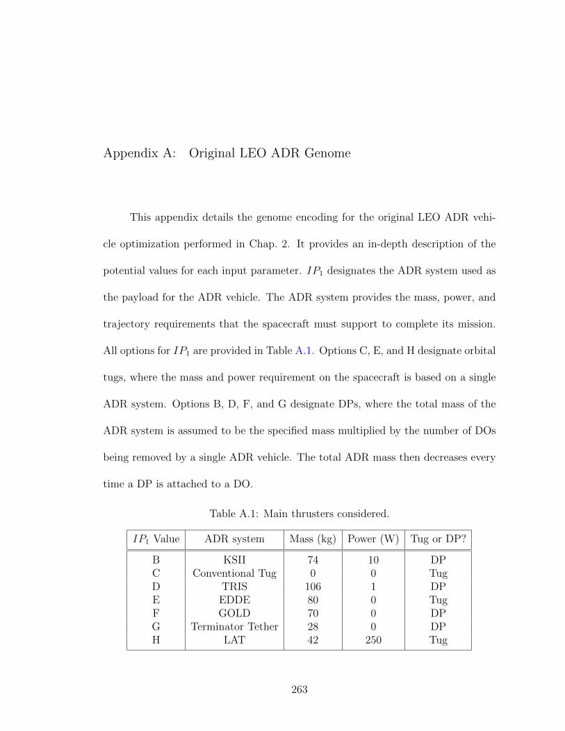
Appendix A: Original LEO ADR Genome
This appendix details the genome encoding for the original LEO ADR vehi-
cle optimization performed in Chap. 2. It provides an in-depth description of the
potential values for each input parameter. IP1 designates the ADR system used as
the payload for the ADR vehicle. The ADR system provides the mass, power, and
trajectory requirements that the spacecraft must support to complete its mission.
All options for IP1 are provided in Table A.1. Options C, E, and H designate orbital
tugs, where the mass and power requirement on the spacecraft is based on a single
ADR system. Options B, D, F, and G designate DPs, where the total mass of the
ADR system is assumed to be the specified mass multiplied by the number of DOs
being removed by a single ADR vehicle. The total ADR mass then decreases every
time a DP is attached to a DO.
Table A.1: Main thrusters considered.
IP1 Value ADR system Mass (kg) Power (W) Tug or DP?
B KSII 74 10 DPC Conventional Tug 0 0 TugD TRIS 106 1 DPE EDDE 80 0 TugF GOLD 70 0 DPG Terminator Tether 28 0 DPH LAT 42 250 Tug
263

IP2 specifies the thruster used as the main propulsion system by the ADR
vehicle. A listing of all thrusters considered is provided below in Table A.2. Bipro-
pellant thrusters are assumed to consume N2H4 and N2O4 as fuel. Monopropellant
thrusters, the resistojet, and arcjets considered use N2H4 as fuel. The resistojet
considered has an Isp of 300s, consumes 900 W of electrical power while running,
produces 0.8145 N of thrust, uses N2H4 as propellant, and has a mass of 0.9 kg. The
PPT considered uses Teflon as propellant, and all Ion engines and Hall thrusters
considered use Xenon.
IP3 designates the number of DOs to be removed by a single ADR vehicle. This
can range anywhere from 1, designating removal of a single DO, to 55, designating
removal of all DOs in the simulated debris belt considered. Some of the ADR
systems considered are capable of propelling the spacecraft independent of the main
thruster.
IP4, IP5, and IP6 designate whether a given maneuver type is performed by
the spacecraft’s ADR system, or by the main thruster. IP4 selects which system
performs maneuvers to raise the ADR vehicles orbit. IP5 selects which system
performs plane change maneuvers. IP6 selects which system performs orbit lowering
maneuvers, performed by tugs with a DO attached. IP4 is only used once by
tender vehicles, and IP6 is unused, since these vehicles do not normally perform
these maneuver types. For each of these input parameters, a value of A indicates
the maneuver is performed by the ADR system, and B indicates the maneuver is
performed by the dedicated propulsion system.
264

IP7 indicates whether a maneuver is considered impulsive or low thrust. Im-
pulsive maneuvers are restricted to 10% of the spacecraft’s orbital period, but require
less ∆V than low thrust maneuvers. For most chemical thrusters, maneuvers are
naturally less than 10% of the spacecraft’s orbital period, so impulsive maneuvers
are naturally superior. For most electrical thrusters, maneuver times are usually
substantially longer than 10% or the spacecraft’s orbital period. As a result, the
necessary ∆V must be broken up into multiple maneuvers, increasing the total
maneuver time by a factor of ten.
IP8 determines whether or not the ADR vehicle takes actions to hold short
of active spacecraft. Much like performing non-impulsive maneuvers, this option
comes with the tradeoff of time spent removing each DO. For orbital tugs, this
action involves holding position above a high priority orbit for some number of days
before crossing it. This allows for safe separation between the ADR spacecraft and
other active spacecraft by waiting for favorable phasing.
IP9 specifies some number of collision avoidance motors to be added to the
ADR vehicle, with the letter value specifying the number of motors. For example,
A designates 0 motors, B designates 1 motor, and so on. The motors are sized so
that they each provide sufficient ∆V to lower the ADR vehicles periapsis by 1 km,
while attached to a DO. These motors allow the ADR vehicle to avoid a short-notice
collision with an active spacecraft.
265
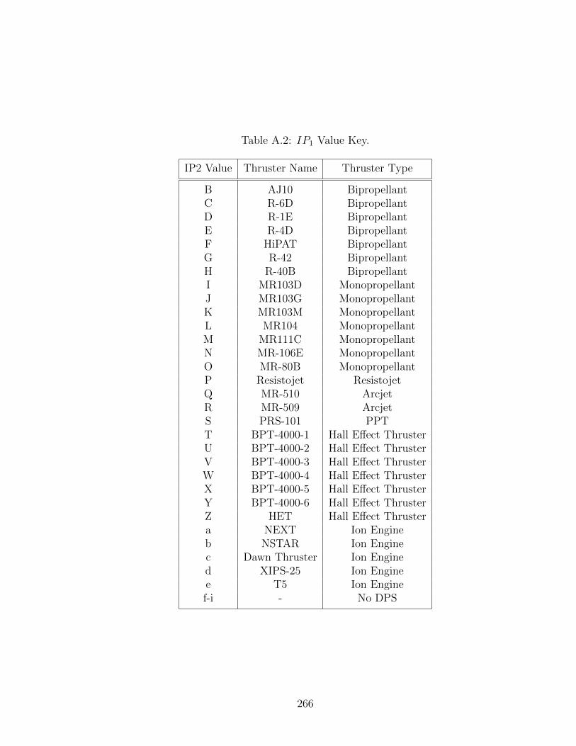
Table A.2: IP1 Value Key.
IP2 Value Thruster Name Thruster Type
B AJ10 BipropellantC R-6D BipropellantD R-1E BipropellantE R-4D BipropellantF HiPAT BipropellantG R-42 BipropellantH R-40B BipropellantI MR103D MonopropellantJ MR103G MonopropellantK MR103M MonopropellantL MR104 MonopropellantM MR111C MonopropellantN MR-106E MonopropellantO MR-80B MonopropellantP Resistojet ResistojetQ MR-510 ArcjetR MR-509 ArcjetS PRS-101 PPTT BPT-4000-1 Hall Effect ThrusterU BPT-4000-2 Hall Effect ThrusterV BPT-4000-3 Hall Effect ThrusterW BPT-4000-4 Hall Effect ThrusterX BPT-4000-5 Hall Effect ThrusterY BPT-4000-6 Hall Effect ThrusterZ HET Hall Effect Thrustera NEXT Ion Engineb NSTAR Ion Enginec Dawn Thruster Ion Engined XIPS-25 Ion Enginee T5 Ion Enginef-i - No DPS
266

Appendix B: Table Design Example Component Libraries
This appendix lists all components, by class, that comprised the component
libraries for the worked example presented in Chap. 5.
B.1 Payload
Only a single payload component was included in this design problem. Its only
property was its mass, which was 100 kg.
B.2 Surfaces
The component properties for all surfaces considered in Chap. 5 are listed in
Table B.1. Surface properties were drawn from the Ikea Table Top Catalog [83].
Table B.1: Real surface properties.
ID model number l (m) w (m) t (m) m (kg) Lmax (N)
1 002.511.35 1 0.6 0.034 5.92 5002 002.513.43 1.2 0.6 0.034 6.4 5003 102.513.52 1.5 0.75 0.034 9.6 5004 501.067.73 1.55 0.75 0.03 26.4 5005 202.406.26 1.2 0.6 0.05 11 500
267

B.3 Real Supports
The component properties for all real supports considered in Chap. 5 are listed
in Table B.2. Properties were drawn from the McMaster-Carr catalog of 80/20
beams and solid 6060 Aluminum rods.
Table B.2: Real support properties.
ID name I (m4) E (Pa) λ (kg/m)
1 8020-30-6060 3.66E-07 7.03E+10 2.572 8020-30-3060 5.55E-08 7.03E+10 1.643 8020-40-4040 1.38E-07 7.03E+10 2.364 8020-25-2525 1.77E-08 7.03E+10 0.745 8020-20-4040 7.84E-08 7.03E+10 1.676 6060 Rod-15mm 7.95E-08 7.00E+10 0.477 6060 Rod-30mm 1.27E-06 7.00E+10 1.91
B.4 Real Supports
The full set of properties for notional support are computed as a function of
material parameters, specified in Table B.3, and level 3 genes, as specified in section
5.4.3.2.
Table B.3: Notional support material properties.
material E (Pa) ρ (kg/m3)
2024 Aluminum 7.30E+10 27804130 Steel 2.05E+11 78506061 Aluminum 6.90E+10 2700Cast Iron – Ductile 1.65E+11 7300Cast Iron – Gray 1.00E+08 7200Stainless Steel 2.00E+11 7950Wood 1.10E+10 750
268
Appendix C: GESDA Component Libraries
This appendix lists all components, by class, that comprised the component
libraries for the implementation of GESDA presented in this dissertation, and used
to produce the results of Chap. 8 and Chap. 9. Payloads are specific to each design
problem, and are fully detailed in their respective chapters, so they are omitted here.
For components with a known flight heritage, a current or previous mission on which
the component was used is prepended to the component name for reference. Unless
otherwise noted, all components are drawn from the NASA SPOON database.
C.1 Data Recorders
The component properties for all data recorders considered in GESDA are
listed in Table C.1. Where no read or write rate is specified, the rate in question is
assumed infinite. That is, it is never limited by the component, only by the net data
flows of the system. In some cases, for the current GESDA implementation, some
complete onboard computers in SPOON whose capabilities include storing science
data were listed here as data recorders.
269

Tab
leC
.1:
Dat
aR
ecor
der
Pro
per
ties
.
nam
em
ass
(kg)
oper
atin
gp
ower
(W)
dat
aca
pac
ity
(bit
s)re
adra
te(b
ps)
wri
tera
te(b
ps)
TR
L
Tac
Sat
3A
iTec
hS99
03.
00E
-01
48.
00E
+09
2.00
E+
082.
00E
+08
9L
AD
EE
Moog
BR
EC
ASI
0.28
4.5
5.12
E+
089
TE
SS
FM
CG
en3
0.68
51.
54E
+12
5.80
E+
086.
15E
+08
9IS
ISiO
BC
0.07
60.
42.
56E
+11
2.40
E+
122.
40E
+12
9Spac
eMic
roF
lash
SSB
0.15
3.5
1.02
E+
129
Xip
hos
Q6
0.01
71
3200
0000
000
2.40
E+
122.
40E
+12
7X
iphos
Q7
0.02
41
2.56
E+
112.
40E
+12
2.40
E+
129
CA
SSIO
PE
Hon
eyw
ell
Dat
aSto
rage
Unit
1256
1.00
E+
123.
50E
+08
4.00
E+
086
Sw
RI
Nex
tgen
Max
wel
l750
7.5
397.
68E
+11
2.00
E+
088.
00E
+07
6L
AD
EE
MO
OG
BR
EM
OA
B0.
356
6.14
E+
095.
00E
+07
5.00
E+
079
MD
AC
DH
1138
1.60
E+
102.
00E
+08
2.00
E+
089
Nig
eria
Sat
2SST
LH
SD
R1
151.
28E
+11
5.00
E+
095.
00E
+09
9Spac
eDynam
ics
PE
AR
L0.
352
9.60
E+
107
SW
RI
PP
CIn
tegr
ated
Avio
nic
s0.
59
1.60
E+
108
AIT
ech
S95
00.
451.
55.
12E
+11
1.04
E+
091.
04E
+09
8G
enes
atA
tmel
AT
45D
B16
1D0.
0002
275
0.02
521.
60E
+07
9SD
LM
OD
AS
320
8.00
E+
092.
00E
+08
2.00
E+
087
Sw
RI
SC
9V
ME
1110
361.
60E
+10
3.00
E+
083.
00E
+08
8W
ISE
FM
CG
en2
0.77
65.
80E
+08
6.15
E+
089
270
C.2 RF Modules
For RF modules, there is a separate component library for each subcomponent
class. Each are listed here in their respective subsections.
C.2.1 Traveling Wave Tube Amplifiers (TWTAs)
All TWTAs used in this work are listed in Table C.2. Properties listed in
include both the TWTA itself and the associated electrical power conditioner. As
modeled, TWTAs do not consider warmup. They are either fully off or fully on in
RF transmit mode. For TWTAs with a range of operating powers, separate versions
of the component operating at maximum and minimum output power were defined.
271
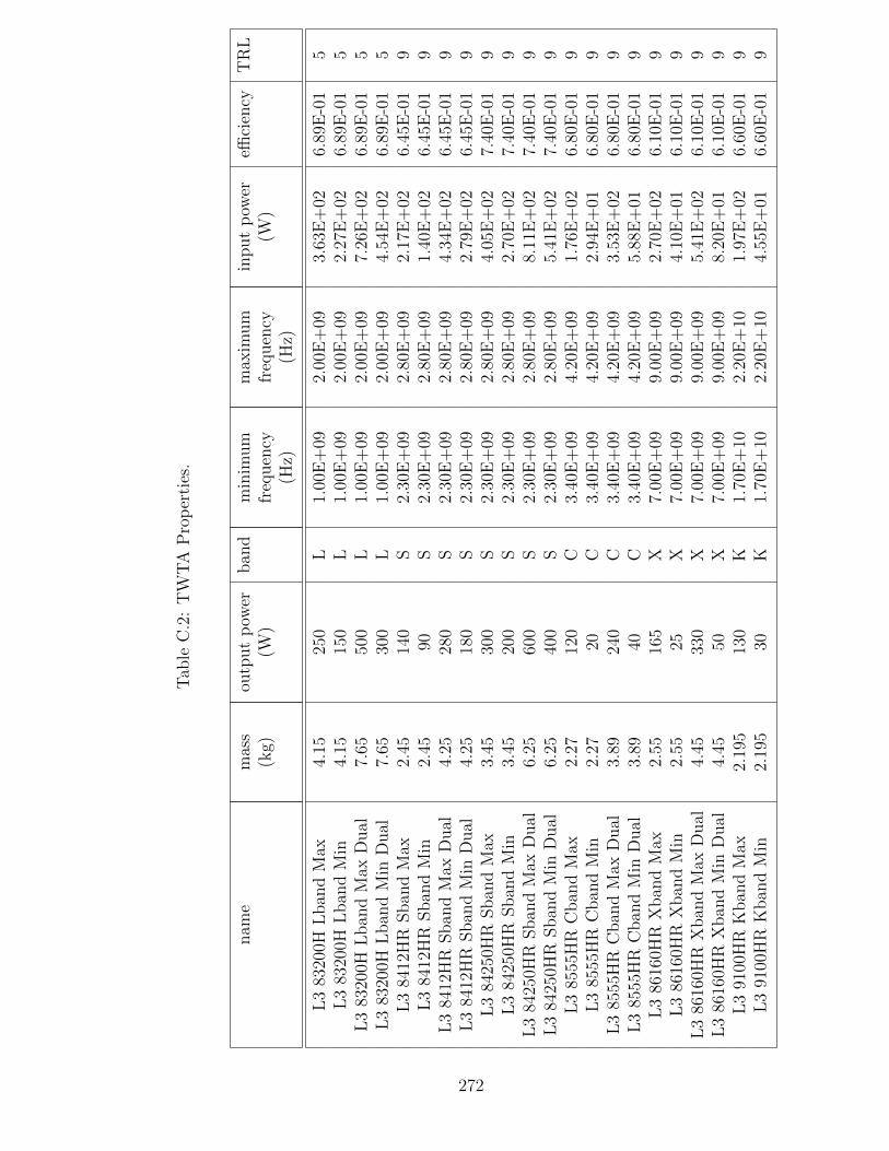
Tab
leC
.2:
TW
TA
Pro
per
ties
.
nam
em
ass
(kg)
outp
ut
pow
er(W
)ban
dm
inim
um
freq
uen
cy(H
z)
max
imum
freq
uen
cy(H
z)
input
pow
er(W
)effi
cien
cyT
RL
L3
8320
0HL
ban
dM
ax4.
1525
0L
1.00
E+
092.
00E
+09
3.63
E+
026.
89E
-01
5L
383
200H
Lban
dM
in4.
1515
0L
1.00
E+
092.
00E
+09
2.27
E+
026.
89E
-01
5L
383
200H
Lban
dM
axD
ual
7.65
500
L1.
00E
+09
2.00
E+
097.
26E
+02
6.89
E-0
15
L3
8320
0HL
ban
dM
inD
ual
7.65
300
L1.
00E
+09
2.00
E+
094.
54E
+02
6.89
E-0
15
L3
8412
HR
Sban
dM
ax2.
4514
0S
2.30
E+
092.
80E
+09
2.17
E+
026.
45E
-01
9L
384
12H
RSban
dM
in2.
4590
S2.
30E
+09
2.80
E+
091.
40E
+02
6.45
E-0
19
L3
8412
HR
Sban
dM
axD
ual
4.25
280
S2.
30E
+09
2.80
E+
094.
34E
+02
6.45
E-0
19
L3
8412
HR
Sban
dM
inD
ual
4.25
180
S2.
30E
+09
2.80
E+
092.
79E
+02
6.45
E-0
19
L3
8425
0HR
Sban
dM
ax3.
4530
0S
2.30
E+
092.
80E
+09
4.05
E+
027.
40E
-01
9L
384
250H
RSban
dM
in3.
4520
0S
2.30
E+
092.
80E
+09
2.70
E+
027.
40E
-01
9L
384
250H
RSban
dM
axD
ual
6.25
600
S2.
30E
+09
2.80
E+
098.
11E
+02
7.40
E-0
19
L3
8425
0HR
Sban
dM
inD
ual
6.25
400
S2.
30E
+09
2.80
E+
095.
41E
+02
7.40
E-0
19
L3
8555
HR
Cban
dM
ax2.
2712
0C
3.40
E+
094.
20E
+09
1.76
E+
026.
80E
-01
9L
385
55H
RC
ban
dM
in2.
2720
C3.
40E
+09
4.20
E+
092.
94E
+01
6.80
E-0
19
L3
8555
HR
Cban
dM
axD
ual
3.89
240
C3.
40E
+09
4.20
E+
093.
53E
+02
6.80
E-0
19
L3
8555
HR
Cban
dM
inD
ual
3.89
40C
3.40
E+
094.
20E
+09
5.88
E+
016.
80E
-01
9L
386
160H
RX
ban
dM
ax2.
5516
5X
7.00
E+
099.
00E
+09
2.70
E+
026.
10E
-01
9L
386
160H
RX
ban
dM
in2.
5525
X7.
00E
+09
9.00
E+
094.
10E
+01
6.10
E-0
19
L3
8616
0HR
Xban
dM
axD
ual
4.45
330
X7.
00E
+09
9.00
E+
095.
41E
+02
6.10
E-0
19
L3
8616
0HR
Xban
dM
inD
ual
4.45
50X
7.00
E+
099.
00E
+09
8.20
E+
016.
10E
-01
9L
391
00H
RK
ban
dM
ax2.
195
130
K1.
70E
+10
2.20
E+
101.
97E
+02
6.60
E-0
19
L3
9100
HR
Kban
dM
in2.
195
30K
1.70
E+
102.
20E
+10
4.55
E+
016.
60E
-01
9
272

nam
em
ass
(kg)
outp
ut
pow
er(W
)ban
dm
inim
um
freq
uen
cy(H
z)
max
imum
freq
uen
cy(H
z)
input
pow
er(W
)effi
cien
cyT
RL
L3
9100
HR
Kban
dM
axD
ual
3.74
260
K1.
70E
+10
2.20
E+
103.
94E
+02
6.60
E-0
19
L3
9100
HR
Kban
dM
inD
ual
3.74
60K
1.70
E+
102.
20E
+10
9.09
E+
016.
60E
-01
9L
399
9HK
ban
dM
ax2.
695
200
Ka
2.20
E+
104.
00E
+10
3.64
E+
025.
50E
-01
9L
399
9HK
aban
dM
in2.
695
20K
a2.
20E
+10
4.00
E+
103.
64E
+01
5.50
E-0
19
L3
999H
Kab
and
Max
Dual
4.74
400
Ka
2.20
E+
104.
00E
+10
7.27
E+
025.
50E
-01
9L
399
9HK
aban
dM
inD
ual
4.74
40K
a2.
20E
+10
4.00
E+
107.
27E
+01
5.50
E-0
19
273

C.2.2 Solid State Amplifiers
All TWTAs used in this work are listed in Table C.3. For any amplifiers for
which no frequency range was specified, it is assumed that their frequency range is
the entire range of their operational bands. For any components without a maxi-
mum data rate specified, their data rate was assumed unlimited (by the component
itself).
274
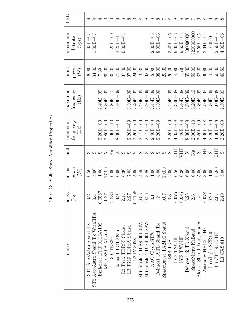
Tab
leC
.3:
Sol
idSta
teA
mplifier
Pro
per
ties
.
nam
em
ass
(kg)
outp
ut
pow
er(W
)
ban
dm
inim
um
freq
uen
cy(H
z)
max
imum
freq
uen
cy(H
z)
input
pow
er(W
)
max
imum
bit
rate
(bps)
TR
L
ST
5A
eroA
stro
Sban
dT
x0.
20.
50S
8.00
1.00
E+
079
ST
5A
eroA
stro
Sban
dT
xW
ithH
PA
0.4
5.00
S34
.00
1.00
E+
079
Em
hei
ser
ET
T01
EB
A10
20.
0567
1.00
S2.
20E
+09
2.40
E+
097.
804
ME
RSSP
AX
ban
d1.
3717
.00
X7.
80E
+09
8.80
E+
0960
.00
9L
3C
TK
830
2.83
40.
00K
a1.
90E
+10
2.80
E+
1030
.00
1.20
E+
099
Ikon
osL
3C
TX
886
3.9
6.00
X8.
00E
+09
8.40
E+
0975
.00
3.20
E+
119
L3
T71
5T
DR
SS
Sban
d2.
176.
30S
37.0
06.
00E
+04
8L
3T
719
TD
RSS
Sban
d2.
277.
08S
2.20
E+
092.
30E
+09
37.0
08
L3
PA
805S
0.11
065.
00S
2.20
E+
092.
40E
+09
24.0
09
Mit
subis
hi
TD
-SS-0
0144
W0.
564.
40S
2.17
E+
092.
20E
+09
16.3
08
Mit
subis
hi
TD
-SS-0
0188
W0.
568.
80S
2.17
E+
092.
20E
+09
32.6
08
AA
CC
lyde
ST
X0.
11.
00S
2.40
E+
092.
45E
+09
5.00
2.00
E+
069
Dei
mos
1SST
LSban
dT
x2
4.00
S2.
20E
+09
2.30
E+
0938
.00
8.00
E+
068
Spac
eQues
tT
X24
00Sban
d0.
0710
.00
S20
.00
7IS
IST
XS
0.3
2.00
S2.
20E
+09
2.29
E+
099.
203.
40E
+06
8IS
IST
XU
HF
0.07
50.
50U
HF
4.35
E+
084.
38E
+08
4.00
9.60
E+
038
ISIS
TX
VH
F0.
085
0.20
VH
F1.
46E
+08
1.46
E+
081.
709.
60E
+03
8D
eim
os1
SST
LX
ban
d3.
256.
00X
8.00
E+
098.
50E
+09
55.0
030
0000
000
8Spac
eMic
roK
aBan
d2.
30.
00K
a2.
00E
+10
3.20
E+
1050
.00
3200
0000
007
Alc
atel
Sban
dT
ransp
onder
45.
00S
2.20
E+
092.
30E
+09
32.0
02.
56E
+05
9A
stro
dev
HE
100
UH
F0.
078
3.00
UH
F4.
00E
+08
4.50
E+
086.
003.
64E
+04
8In
nofl
ight
SC
R10
00.
291.
00S
2.20
E+
092.
30E
+09
10.0
010
0000
9L
3C
TT
505
UH
F2.
0713
.80
UH
F4.
00E
+08
5.00
E+
0860
.00
2.56
E+
058
L3
CX
S61
02.
495.
00S
2.20
E+
092.
30E
+09
40.5
04.
00E
+06
8
275
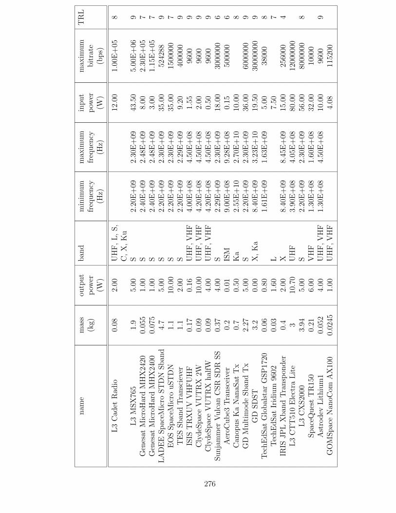
nam
em
ass
(kg)
outp
ut
pow
er(W
)
ban
dm
inim
um
freq
uen
cy(H
z)
max
imum
freq
uen
cy(H
z)
input
pow
er(W
)
max
imum
bit
rate
(bps)
TR
L
L3
Cad
etR
adio
0.08
2.00
UH
F,
L,
S,
C,
X,
Ku
12.0
01.
00E
+05
8
L3
MSX
765
1.9
5.00
S2.
20E
+09
2.30
E+
0943
.50
5.00
E+
069
Gen
esat
Mic
roH
ard
MH
X24
200.
055
1.00
S2.
40E
+09
2.48
E+
098.
002.
30E
+05
7G
enes
atM
icro
Har
dM
HX
2400
0.07
51.
00S
2.40
E+
092.
48E
+09
3.00
1.15
E+
057
LA
DE
ESpac
eMic
roST
DN
Sban
d4.
75.
00S
2.20
E+
092.
30E
+09
35.0
052
4288
9E
OS
Spac
eMic
rouST
DN
1.1
10.0
0S
2.20
E+
092.
30E
+09
35.0
015
0000
07
TE
SSban
dT
ransc
ieve
r1.
12.
00S
2.20
E+
092.
29E
+09
9.20
4000
009
ISIS
TR
XU
VV
HF
UH
F0.
170.
16U
HF
,V
HF
4.00
E+
084.
50E
+08
1.55
9600
9C
lydeS
pac
eV
UT
RX
2W0.
0910
.00
UH
F,V
HF
4.20
E+
084.
50E
+08
2.00
9600
9C
lydeS
pac
eV
UT
RX
hal
fW0.
094.
00U
HF
,V
HF
4.20
E+
084.
50E
+08
0.50
9600
9Sunja
mm
erV
ulc
anC
SR
SD
RSS
0.37
4.00
S2.
29E
+09
2.30
E+
0918
.00
3000
000
6A
eroC
ub
e3T
ransc
eive
r0.
20.
01IS
M9.
00E
+08
9.28
E+
080.
1550
0000
6C
anop
us
Ka
Nan
aSat
Tx
0.7
0.50
Ka
2.55
E+
102.
70E
+10
10.0
08
GD
Mult
imode
Sban
dT
x2.
275.
00S
2.20
E+
092.
30E
+09
36.0
060
0000
09
GD
SD
ST
3.2
0.00
X,
Ka
8.40
E+
093.
23E
+10
19.5
030
0000
009
Tec
hE
dSat
Glo
bal
star
GSP
1720
0.06
0.80
1.61
E+
091.
63E
+09
5.00
3800
08
Tec
hE
dSat
Irid
ium
9602
0.03
1.60
L7.
507
IRIS
JP
LX
ban
dT
ransp
onder
0.4
2.00
X8.
40E
+09
8.45
E+
0915
.00
2560
004
L3
CT
T51
0E
lect
raL
ite
310
.70
UH
F3.
90E
+08
4.05
E+
0880
.00
1200
0000
L3
CX
S20
003.
945.
00S
2.20
E+
092.
30E
+09
56.0
080
0000
08
Spac
eQues
tT
R15
00.
216.
00V
HF
1.30
E+
081.
60E
+08
32.0
010
000
Ast
rodev
Lit
hiu
m1
0.05
24.
00U
HF
,V
HF
1.30
E+
084.
50E
+08
10.0
096
009
GO
MSpac
eN
anoC
omA
X10
00.
0245
1.00
UH
F,V
HF
4.08
1152
00
276
C.2.3 Low Gain Antennas (LGAs)
Approximately half of the LGA data was drawn from SPOON. Of the other
half, much was drawn from JPL’s Deep Space Communications and Navigation
Systems Center, DESCANSO, with some components drawn from a number of other
technical sources. Components drawn from SPOON are listed in Table C.4. Those
from other sources are listed in Table C.5, along with the source documents for
each. No TRL was assigned for non-SPOON LGAs. For these, a default TRL of 6
was assumed. Additionally, bands were not specified for these components. As a
result, compatible bands were determined based on the frequency ranges for each
component.
277

Tab
leC
.4:
LG
As
from
SP
OO
N.
nam
em
ass
(kg)
dow
nlink
gain
(dB
)
uplink
gain
(dB
)
ban
db
eam
wid
th(d
eg)
max
imum
input
pow
er(d
B)
TR
L
AD
CM
icro
stri
pST
DN
sban
dsi
ngl
ef0.
1611
.811
.8S
408
MO
ST
AD
CX
ban
dQ
uad
Hel
ixL
EO
0.22
22
X16
012
8Sta
rdust
AD
Cxban
dhor
n0.
821
21X
1410
9A
DC
MG
AP
atch
linea
r0.
155
10.5
10.5
L,
S,
C,
X45
147
AD
CM
GA
Pat
chci
rcula
r0.
155
10.5
10.5
L,
S,
C,
X45
147
Gen
esis
AD
CM
icro
stri
pP
atch
xban
dlinea
r0.
086
6X
7010
8G
enes
isA
DC
Mic
rost
rip
Pat
chxban
dci
rcula
r0.
086
6X
7010
8G
enes
isA
DC
Mic
rost
rip
Pat
chsb
and
linea
r0.
086
6S
8010
8G
enes
isA
DC
Mic
rost
rip
Pat
chsb
and
circ
ula
r0.
086
6S
8010
8A
stro
Dev
Sban
dP
atch
0.00
43
2S
120
4.77
8IS
ISD
eplo
yable
UH
F0.
010
0U
HF
,V
HF
453
8R
UA
GK
aP
ipe
0.01
98
8K
a80
10M
aruw
aSL
3101
0.02
92
2L
120
37
Phon
eSat
Mon
opol
eU
HF
0.01
50
0U
HF
903
7R
UA
GSban
dH
elix
0.28
4S
5510
RU
AG
Sban
dT
TC
Hel
ix0.
253
3S
40R
UA
GSban
dO
mni
0.75
33
S18
0Surr
eyX
ban
dH
orn
2.7
1515
X20
209
ST
5E
AA
nte
nna
0.16
53
X7
Tao
glas
WL
P.2
450.
25.4
.A0.
055
5S
609
6R
UA
GX
ban
dp
ec0.
016
77
X90
10ST
5A
DC
Quad
Hel
ixX
ban
d0.
222
2X
107
278

Tab
leC
.5:
LG
As
from
other
sourc
es.
nam
em
ass
gain
(dB
)m
inim
um
freq
uen
cy(H
z)
max
imum
freq
uen
cy(H
z)
bea
mw
idth
(deg
)
max
imum
input
pow
er(W
)
sourc
e
Cas
sini
LG
A1
0.5
8.94
8.43
E+
098.
43E
+09
24[8
4]C
assi
ni
LG
A2
0.5
98.
43E
+09
8.43
E+
0940
[84]
DA
WN
LG
A0.
56
7.17
E+
098.
45E
+09
90[8
5]D
eepIm
pac
tL
GA
10.
063
8.44
E+
098.
44E
+09
90[8
6]IS
EE
-C0.
957
2.22
E+
092.
27E
+09
1213
[87]
Om
ni
AS-4
8915
0.31
24
1.75
E+
092.
30E
+09
4510
[88]
ISE
E-A
0.95
32.
22E
+09
2.26
E+
0960
13[8
7]IS
EE
-C0.
957
2.22
E+
092.
27E
+09
1213
[87]
Juno
MG
A0.
518
.87.
15E
+09
8.40
E+
0918
.6[8
6]Juno
TL
GA
1.9
6.5
7.15
E+
098.
40E
+09
20[8
6]M
arsO
dyss
eyL
GA
0.04
77.
16E
+09
7.16
E+
0982
[86]
MR
OE
lect
raA
nte
nna
1.4
54.
37E
+08
4.37
E+
0870
[86]
MR
OL
GA
0.8
8.8
7.15
E+
098.
44E
+09
80[8
6]Shap
edO
mni
(NA
SA
-TR
-100
680)
2.27
02.
09E
+09
2.31
E+
0917
010
[87]
SA
AB
LC
RO
SS
PE
C0.
325
12.5
1.98
E+
092.
20E
+09
50[8
9]SA
AB
XH
elix
60E
OC
0.4
27.
25E
+09
8.40
E+
0916
0[8
9]SM
AP
SL
GA
0.25
02.
00E
+09
2.30
E+
0919
010
[86]
SM
AP
XL
GA
0.4
1.5
8.03
E+
098.
33E
+09
160
10[8
6]
279

C.2.4 High Gain Antennas (HGAs)
HGAs were drawn primarily from DESCANSO. Their properties are listed in
Table C.6. All are assumed to be parabolic reflectors. Like with the LGAs drawn
from non-SPOON sources, no TRL was assigned for non-SPOON LGAs. TRL and
communications bands were assigned as specified for LGAs.
Table C.6: HGAs considered.
name mass(kg)
nominalgain(dB)
nominalwavelength
(m)
diameter(m)
source
Cassini HGAS 100.6 46.6 0.035583675 4 [90]Dawn HGA 7 39.6 0.035539928 1.524 [85]
Deep Impact HGA 2.8 35.6 0.035541489 1 [91]Juno HGA 21.3 44.5 0.035672015 2.5 [92]LRO HGAS 50.1 44 0.011687815 0.75 [93]
Mars Odyssey HGAS 3.15 38.3 0.03566049 1.3 [84]MRO HGAS 65.7 56.4 0.009368514 3 [94]
Voyager HGAS 53 48 0.035602978 3.66 [95]
C.3 Solar Panels (PVAs)
A subset of PVAs, given in Table C.7, was used in Chap. 8. In Chap. 9, the
additional PVAs in Table C.8 were considered as well. The final six components in
Table C.8 are artificially created macrocomponents.
C.4 Batteries
All batteries considered are listed in Table C.9. Data is drawn primarily from
SPOON. For EnerSys batteries, additional data was drawn from [96].
280

Table C.7: PVAs considered in Chap. 8.
name mass (kg) efficiency area (m2) TRL
DHV CS 10 0.05 2.19E-01 8.09E-03 7EXA DSA 1A 1panel NEMEA highpower 0.067 6.48E-01 8.13E-03 9
EXA DSA 1A 1panel NEMEA lowcost 0.067 2.47E-01 8.13E-03 9EXA DSA 1A 1panel noNEMEA highpower 0.057 6.48E-01 8.13E-03 9
EXA DSA 1A 1panel noNEMEA lowcost 0.057 2.47E-01 8.13E-03 9EXA DSA 1A 2panels NEMEA highpower 0.115 5.93E-01 1.48E-02 9
EXA DSA 1A 2panels NEMEA lowcost 0.115 2.12E-01 1.48E-02 9EXA DSA 1A 2panels noNEMEA highpower 0.087 5.93E-01 1.48E-02 9
EXA DSA 1A 2panels noNEMEA lowcost 0.087 2.12E-01 1.48E-02 9EXA DSA 1A 3panels NEMEA highpower 0.135 5.72E-01 2.15E-02 9
EXA DSA 1A 3panels NEMEA lowcost 0.135 2.13E-01 2.15E-02 9EXA DSA 1A 3panels noNEMEA highpower 0.107 5.72E-01 2.15E-02 9
EXA DSA 1A 3panels noNEMEA lowcost 0.107 2.13E-01 2.15E-02 9ISIS 1U PVA 0.05 0.208 0.00809 9ISIS 2U PVA 0.1 0.208 0.0162 9ISIS 3U PVA 0.15 0.208 0.0243 9ISIS 6U PVA 0.3 0.256 0.0485 9
C.5 Thrusters
All thrusters used were drawn from the original component library from the
work of [76]. Where available, this data was supplemented with data from SPOON.
C.6 Propellant Tanks
All liquid propellant types had component libraries based on the same set of
tank components, given in Table C.11. Xenon tanks were based on a separate list of
gaseous tank components, given in Table C.12. All tanks were drawn from SPOON.
281
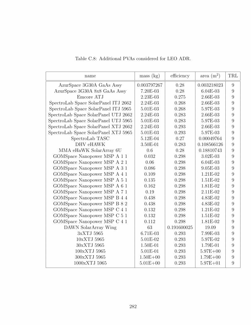
Table C.8: Additional PVAs considered for LEO ADR.
name mass (kg) efficiency area (m2) TRL
AzurSpace 3G30A GaAs Assy 0.003797267 0.28 0.003218023 9AzurSpace 3G30A 8x8 GaAs Assy 7.20E-03 0.28 6.04E-03 9
Emcore ATJ 2.23E-03 0.275 2.66E-03 9SpectroLab Space SolarPanel ITJ 2662 2.24E-03 0.268 2.66E-03 9SpectroLab Space SolarPanel ITJ 5965 5.01E-03 0.268 5.97E-03 9SpectroLab Space SolarPanel UTJ 2662 2.24E-03 0.283 2.66E-03 9SpectroLab Space SolarPanel UTJ 5965 5.01E-03 0.283 5.97E-03 9SpectroLab Space SolarPanel XTJ 2662 2.24E-03 0.293 2.66E-03 9SpectroLab Space SolarPanel XTJ 5965 5.01E-03 0.293 5.97E-03 9
SpectroLab TASC 5.12E-04 0.27 0.00049764 9DHV eHAWK 3.50E-01 0.283 0.108566126 9
MMA eHaWK SolarArray 6U 0.6 0.28 0.18810743 9GOMSpace Nanopower MSP A 1 1 0.032 0.298 3.02E-03 9GOMSpace Nanopower MSP A 2 1 0.06 0.298 6.04E-03 9GOMSpace Nanopower MSP A 3 1 0.086 0.298 9.05E-03 9GOMSpace Nanopower MSP A 4 1 0.109 0.298 1.21E-02 9GOMSpace Nanopower MSP A 5 1 0.135 0.298 1.51E-02 9GOMSpace Nanopower MSP A 6 1 0.162 0.298 1.81E-02 9GOMSpace Nanopower MSP A 7 1 0.19 0.298 2.11E-02 9GOMSpace Nanopower MSP B 4 4 0.438 0.298 4.83E-02 9GOMSpace Nanopower MSP B 8 2 0.438 0.298 4.83E-02 9GOMSpace Nanopower MSP C 4 1 0.132 0.298 1.21E-02 9GOMSpace Nanopower MSP C 5 1 0.132 0.298 1.51E-02 9GOMSpace Nanopower MSP C 4 1 0.112 0.298 1.81E-02 9
DAWN SolarArray Wing 63 0.191600025 19.09 93xXTJ 5965 6.71E-03 0.293 7.99E-03 910xXTJ 5965 5.01E-02 0.293 5.97E-02 930xXTJ 5965 1.50E-01 0.293 1.79E-01 9100xXTJ 5965 5.01E-01 0.293 5.97E+00 9300xXTJ 5965 1.50E+00 0.293 1.79E+00 91000xXTJ 5965 5.01E+00 0.293 5.97E+01 9
282
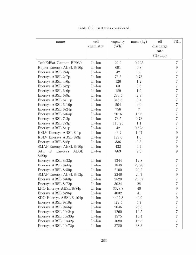
Table C.9: Batteries considered.
name cellchemistry
capacity(Wh)
mass (kg) self-discharge
rate(%/day)
TRL
TechEdSat Cannon BP930 Li-Ion 22.2 0.225 7Kepler Enersys ABSL 8s16p Li-Ion 691 6.8 9Enersys ABSL 2s4p Li-Ion 42 0.6 7Enersys ABSL 2s7p Li-Ion 73.5 0.73 7Enersys ABSL 4s6p Li-Ion 126 1.2 7Enersys ABSL 6s2p Li-Ion 63 0.6 7Enersys ABSL 6s6p Li-Ion 189 1.9 7Enersys ABSL 6s9p Li-Ion 283.5 2.8 7Enersys ABSL 6s11p Li-Ion 346.5 3.4 7Enersys ABSL 6s16p Li-Ion 504 4.9 7Enersys ABSL 6s24p Li-Ion 756 7 7Enersys ABSL 6s64p Li-Ion 2016 18.6 7Enersys ABSL 7s2p Li-Ion 73.5 0.73 7Enersys ABSL 7s3p Li-Ion 110.25 1.1 7Enersys ABSL 8s1p Li-Ion 42 0.625 7KSLV Enersys ABSL 8s1p Li-Ion 43.2 1.07 9KSLV Enersys ABSL 8s3p Li-Ion 129.6 1.6 9Enersys ABSL 8s8p Li-Ion 336 3.3 7SMAP Enersys ABSL 8s10p Li-Ion 432 4.4 9SAC D Enersys ABSL8s20p
Li-Ion 863 9.3 9
Enersys ABSL 8s32p Li-Ion 1344 12.8 7Enersys ABSL 8s44p Li-Ion 1848 20.98 7Enersys ABSL 8s50p Li-Ion 2100 20.2 7SMAP Enersys ABSL 8s52p Li-Ion 2246 20.7 9Enersys ABSL 8s60p Li-Ion 2520 28.37 7Enersys ABSL 8s72p Li-Ion 3024 28 7LRO Enersys ABSL 8s84p Li-Ion 3628.8 40 9Enersys ABSL 8s96p Li-Ion 4032 41 7SDO Enersys ABSL 8s104p Li-Ion 4492.8 49.9 9Enersys ABSL 9s10p Li-Ion 472.5 4.7 7Enersys ABSL 9s56p Li-Ion 2646 25.5 7Enersys ABSL 10s24p Li-Ion 1260 12.5 7Enersys ABSL 10s30p Li-Ion 1575 16.4 7Enersys ABSL 10s32p Li-Ion 1680 16.8 7Enersys ABSL 10s72p Li-Ion 3780 38.3 7
283

name cellchemistry
capacity(Wh)
mass (kg) self-discharge
rate(%/day)
TRL
Enersys ABSL 12s24p Li-Ion 518.4 14.4 7Enersys ABSL 12s28p Li-Ion 697.2 16.6 7Enersys ABSL 16s16p Li-Ion 1344 14.5 7Enersys ABSL 84s2p Li-Ion 882 11.5 7Enersys ABSL 3s4p Li-Ion 125 0.98 7CS 1U LiPo 10 0.062GomSpace 1800mAh bat-tery
Li-Ion 13.32 0.095 0.00001 9
GomSpace BP4 2p2s Li-Ion 38.5 0.258 8GomSpace BP4 1p4s Li-Ion 38.5 0.258 8Mitsubishi 5kW LI battery Li-Ion 8620 81 0.001 8Genesat Rose LiIon2200mAh
Li-Ion 16.2 0.098 9
Saft 60145B 8s LD25P Li-Ion 162 2.2 0.0024161GIOVEB Saft VES 100 Li-Ion 95.6 0.81 9Saft VL48E Li-Ion 172.5 1.15Sony 18650 Li-Ion 5.4 0.042 9SpaceQuest BAT 4 Li-Ion 4.9 0.16 7X37B Yardney Lithion9553HV
Li-Ion 1814 26.3 6
MarsLander YardneyLithion LP3028
Li-Ion 950.4 17.8 7
X37 Yardney LP30950 Li-Ion 1238.4 13.5MER Yardney LP30990 Li-Ion 604.8 7.9 9Yardney LP31685 Li-Ion 1238.4 12.62Yardney NCP05 Li-Ion 0.24 0.004Yardney NCP25 1 Li-Ion 129 0.89Yardney NCP25 2 Li-Ion 95 0.908Yardney NCP3501 Li-Ion 1414 6.67 0.0001Yardney NCP431 Li-Ion 180 1.27 0.0001Yardney NCP552 Li-Ion 198 1.582 0.0001NASA CBSF B79010 10 Li-S 900 3.8555 5.50E-05 5CS Standalone 30Whr LiPo 30 0.26 0.005 8GOMSpace NanopowerP31u s2p
Li-Ion 20 0.2 9
LG ICR18650 Li-Ion 10.5 0.047 0.003 7CS LiPo 6 25 Ah LiPo 150 1 8Mitsubishi 4.4kw LIB0003a Li-Ion 7560 67.2 0.001 8Orbtronic 18650 Li-Ion 12.2 0.046
284

name cellchemistry
capacity(Wh)
mass (kg) self-discharge
rate(%/day)
TRL
Genesat Rose LiIon4400mAh
Li-Ion 32.4 0.19 9
Saft 15s3p MPS176065 Li-Ion 1125 9.9 7Saft VES140 Li-Ion 142.38 1.13 9Saft VES180 Li-Ion 194.25 1.11 9Samsung 18650 Li-Ion 9.33 0.048 9XSS11 Yardney LithionLP31105
Li-Ion 864 9.18 9
SpectrumAstro YardneyLithion LP31280
Li-Ion 1728 20.32
NextSat Yardney LithionLP31500
Li-Ion 864 11.35
Yardney LP30588 Li-Ion 43 0.422 0.0001Yardney NCP7 Li-Ion 27 0.245 0.0001
285

Table C.10: Thrusters considered.
name mass Isp Ft Pon (W) prop1 f1 prop2 f2 TRL
R-4D 4.31 316 489 46 MMH 1 NTO 1.73 9AJ10 100 320 44000 0 Aerozine50 1 NTO 1.9 9R-6D 0.454 294 22 5 MMH 1 NTO 1.65 9R-1E 2 280 111 36 MMH 1 NTO 0.85 9
HiPAT 5.44 323 445 46 MMH 1 NTO 0.85 9R-42 4.53 303 890 46 MMH 1 NTO 1.73 9
R-40B 6.8 293 4000 70 MMH 0.52 NTO 0.838 9MR103D 0.33 217 1.02 8.25 N2H4 1 9MR103G 0.33 213 1.13 8.25 N2H4 1 9MR103M 0.16 213 0.99 7.1 N2H4 1 9MR104 1.86 240 440 30 N2H4 1 9
MR111C 0.33 222 4 8.25 N2H4 1 9MR-106E 0.635 232 22 25.3 N2H4 1 9MR-80B 8.51 200 3100 168 N2H4 1 9MR-502 0.9 300 0.8145 900 N2H4 1 9MR-510 5.5 585 0.23 2200 N2H4 1 9MR-509 5.5 502 0.23 1800 N2H4 1 8PRS-101 4.75 1350 0.0125 1350 Teflon 1 9
BPT-4000-1 25 1676 1.32E-01 2000 Xenon 1 9BPT-4000-2 25 1700 0.195 3000 Xenon 1 9BPT-4000-3 25 1790 0.29 4500 Xenon 1 9BPT-4000-4 25 1858 0.117 2000 Xenon 1 9BPT-4000-5 25 1920 0.17 3000 Xenon 1 9BPT-4000-6 25 2020 0.254 4500 Xenon 1 9
NEXT 47.2 4190 0.236 7200 Xenon 1 6NSTAR 25.5 3200 0.08 1950 Xenon 1 9
DawnThruster 23.34 3100 0.092 2500 Xenon 1 9XIPS-25 37 3400 0.165 4500 Xenon 1 9
T5 20 3200 0.018 476 Xenon 1 9
286

Table C.11: Liquid propellant tanks considered.
name mass (kg) fill volume (L) TRL
ATK PSI 80225-1 3.701 22.532 9ATK PSI 80228-1 19.958 132.079 9ATK PSI 80276-1 4.309 30.152 9ATK PSI 80285-1 6.985 33.577 9ATK PSI 80290-1 2.54 12.454 9ATK PSI 80315-1 44.452 458.837 9ATK PSI 80323-1 14.288 113.398 9ATK PSI 80348-1 19.504 167.393 9ATK PSI 80362-1 7.348 72.574 9ATK PSI 80373-1 13.834 337.229 9ATK PSI 80388-1 7.03 72.574 9ATK PSI 80389-1 3.719 22.532 9ATK PSI 80453-1 7.03 72.27 9ATK PSI 80512-1 6.01 45.03 9ATK PSI 80156-1 1.319 4.752 9ATK PSI 80222-1 1.292 4.752 9ATK PSI 80275-1 5.76 32.036 9ATK PSI 80339-1 13.653 249.022 9ATK PSI 80356-1 27.215 438.353 9ATK PSI 80364-1 5.669 68.038 9ATK PSI 80376-1 34.473 345.898 9Ariane5 BT01 0 8.5 39 9
Globalstar OST31 1 6.4 78 9MicroAerospaceSolutions Tank 0.11 0.03 6
ATK PSI 80216-1 2.721 12.454 9ATK PSI 80263-201 34.473 345.898 9ATK PSI 80266-1 2.222 12.454 9ATK PSI 80287-1 19.05 157.512 9ATK PSI 80303-1 5.896 32.167 9
Skynet ATK PSI 80308-101 5.624 37.648 9ATK PSI 80319-101 5.987 28.267 9ATK PSI 80342-1 2.721 14.453 9ATK PSI 80358-1 5.896 32.2 9ATK PSI 80360-1 5.669 65.77 9ATK PSI 80370-1 34.473 345.898 9ATK PSI 80375-1 8.618 114.758 9ATK PSI 80392-1 5.624 37.648 9ATK PSI 81214-1 3.583 24.826 9ATK PSI 80271-3 5.17 24.908 9ATK PSI 80273-3 12.246 55.224 9
287

name mass (kg) fill volume (L) TRL
ATK PSI 80274-1 6.01 45.031 9ATK PSI 80281-3 9.071 101.567 9ATK PSI 80297-1 19.504 141.715 9ATK PSI 80304-1 3.515 38.493 9ATK PSI 80325-1 19.958 132.079 9ATK PSI 80337-1 6.35 28.267 9ATK PSI 80359-1 6.985 25.973 9ATK PSI 80359-1 34.518 345.898 9ATK PSI 80359-1 7.03 72.574 9
ATK PSI 80263-101 34.473 345.898 9ATK PSI 80280-103 10.659 73.886 9ATK PSI 80298-1 9.525 8.178 9ATK PSI 80309-1 8.073 149.415 9ATK PSI 80353-1 3.855 58.583 9ATK PSI 80384-1 5.896 32.2 9
288

Table C.12: Gaseous tanks considered.
name mass (kg) fill volume (L) max pressure (Pa) TRL
ATK PSI 80186-1 10.569 28.86 2.50E+07 9ATK PSI 80198-1 7.666 18.8 2.50E+07 9ATK PSI 80374-1 9.979 67.27 3.10E+07 9Aerojet Plenum 0.072 0.033 8.96E+06 9
Shuttle Arde C4284-2 0.517 0.983 2.07E+07 9X33 C4683 4.309 13.32 2.21E+07 6
Shuttle Arde D4051 0.916 2.933 7.24E+06 9Shuttle Arde D4554 30.391 132.08 3.10E+07 9
Arde D4607 24.948 85.29 2.76E+07 6Arde D4619 18.28 96.96 3.10E+07 9
ATK PSI 80119-105 0.839 7.489 4.14E+06 9ATK PSI 80194-1 5.375 15.65 2.48E+07 9
ATK PSI 80314-201 16.012 36.05 2.48E+07 9Cassini Arde D4575 3.357 6.55 2.48E+07 9
ISS Arde D4636 7.711 27.53 2.07E+07 9SAFER Arde D4639 1.769 2.79 6.89E+07 9Olympus Arde E4070 10.206 30.81 2.76E+07 9
GOES Arde E4256 19.731 75.34 2.76E+07 9Eurostar EADS LV 35 5L 7.8 35.5 2.76E+07 9
ATK PSI 80221-1 24.857 87.31 2.07E+06 9ATK PSI 80295-1 1.451 1.639 5.52E+07 9ATK PSI 80326-1 1.533 3.851 2.48E+07 9ATK PSI 80383-1 16.012 36.05 2.48E+07 9
Arde D3961 0.807 0.9 4.14E+07 9UoSat Arde D4598 4.899 9.996 2.07E+07 9
UoSat Arde D4600-1 0.916 1.311 4.14E+06 9ISS Arde D4708 1.5 2.868 2.07E+07 9EADS LV110L 23 110 3.10E+07 8
ATK PSI 80202-1 7.167 14.519 3.10E+07 9ATK PSI 80333-1 36.242 105.7 2.80E+07 9
ATK PSI 80458-101 19.05 119.63 1.86E+07 9
289

name mass (kg) fill volume (L) max pressure (Pa) TRL
Shuttle Arde C4285-1 0.517 1.311 2.07E+07 9IABS Arde D4307 10.659 51.73 3.10E+07 9
Arde D4678 2.268 1.88 2.21E+07 9Shuttle Arde D4097 2.903 14.257 4.24E+06 9
ISS Arde D4406 3.538 13.88 8.27E+06 9Dawn Carleton 7169 22.2 268 8.62E+06 9
EADS LV18 3L 4.3 18.3 2.65E+07 9EADS LV300L 81 300 4.00E+07 9EADS LV51L 11.5 51 2.95E+07 9EADS LV80L 17.7 80 3.10E+07 9
ATK PSI 80195-1 5.443 9.373 1.84E+07 9ATK PSI 80345-1 3.357 6.555 3.10E+07 9
Arde D4600-3 0.816 0.869 4.14E+06 9Rosetta EADS LV68L 15.6 68 3.10E+07 9
290
Appendix D: DOVE Simulation Data
This appendix lists all access data used during the simulation described in
Chap. 8. Each section below contains data from a given station. Each table within
a section gives data on a given pass for that station. In each table, time is measured
in elapsed seconds since the beginning of the simulation. Properties at a given
simulation timestep during an access window are linearly interpolated between the
nearest points given in the appropriate table. Elevation angles are measured from
the spacecraft to the station. As a result, all elevation angles are negative for ground
stations.
291

D.1 SG1 (Svalbard)
elapsed time(s)
range(km)
elevation(degrees)
897.855 2548.775 -21.746957 2154.629 -22.0951017 1769.159 -23.361077 1412.368 -26.0351137 1114.423 -30.5261197 935.210 -35.2711257 945.684 -34.9661317 1140.528 -30.0891377 1446.412 -25.7931437 1806.806 -23.291497 2193.793 -22.132
1552.685 2565.077 -21.843
elapsed time(s)
range(km)
elevation(degrees)
6580.262 2551.140 -21.7586640 2206.744 -22.0236700 1894.455 -22.8396760 1636.911 -24.1646820 1464.616 -25.5626880 1409.965 -26.1376940 1486.160 -25.4027000 1675.095 -23.9917060 1943.442 -22.757120 2262.136 -22.034
7172.303 2565.562 -21.847
292
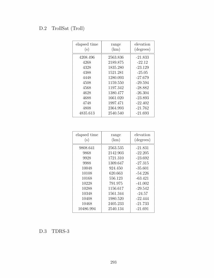
D.2 TrollSat (Troll)
elapsed time(s)
range(km)
elevation(degrees)
4208.496 2563.836 -21.8334268 2189.875 -22.124328 1835.280 -23.1294388 1521.281 -25.054448 1280.093 -27.6794508 1159.550 -29.5944568 1197.342 -28.8824628 1380.477 -26.3044688 1661.020 -23.8934748 1997.471 -22.4024808 2364.993 -21.762
4835.613 2540.540 -21.693
elapsed time(s)
range(km)
elevation(degrees)
9808.641 2563.535 -21.8319868 2142.903 -22.2059928 1721.310 -23.6929988 1309.647 -27.31510048 924.450 -35.60110108 620.663 -54.22610168 556.123 -63.42110228 791.975 -41.00210288 1156.617 -29.54210348 1561.344 -24.5710408 1980.520 -22.44410468 2405.233 -21.733
10486.994 2540.134 -21.691
D.3 TDRS-3
293

elapsed time(s)
range(km)
elevation(degrees)
0 35282.231 -86.960 35279.220 -86.915120 35303.669 -86.798180 35355.433 -86.566240 35434.217 -86.244300 35539.576 -85.859360 35670.924 -85.434420 35827.536 -84.987480 36008.566 -84.532540 36213.046 -84.079600 36439.908 -83.635660 36687.990 -83.207720 36956.047 -82.799780 37242.768 -82.414840 37546.784 -82.056900 37866.682 -81.726960 38201.016 -81.4261020 38548.316 -81.1581080 38907.098 -80.9221140 39275.875 -80.7181200 39653.164 -80.5471260 40037.493 -80.411320 40427.404 -80.3041380 40821.466 -80.2311440 41218.274 -80.191500 41616.454 -80.181560 42014.669 -80.21620 42411.618 -80.251680 42806.040 -80.3281740 43196.719 -80.4341800 43582.479 -80.5651860 43962.190 -80.7231920 44334.770 -80.9041980 44699.178 -81.108
2031.39 45004.045 -81.3
294
Bibliography
[1] B. Randolph, W. Hreha, and A. Q. Rogers, “Key technology, programmaticdrivers, and lessons learned for production of proliferated small satellite con-stellations,”
[2] B. Doncaster, J. Shulman, J. Bradford, and J. Olds, “Spaceworks’ 2016nano/microsatellite market forcast,” in Proceedings of the 30th annualAIAA/USU Conference on Small Satellites, vol. 30, 2016.
[3] V. L. Foreman, A. Siddiqi, and O. De Weck, “Large satellite constellationorbital debris impacts: Case studies of oneweb and spacex proposals,” in AIAASPACE and Astronautics Forum and Exposition, p. 5200, 2017.
[4] J. Radtke, E. Stoll, H. Lewis, and B. B. Virgili, “The impact of the increasein small satellite launch traffic on the long-term evolution of the space debrisenvironment,” in Proc. 7th European Conference on Space Debris, 2017.
[5] Space Exploration Holdings, LLC, “Spacex non-geostationary satellite system- technical attachment,” November 2016.
[6] Space Exploration Holdings, LLC, “Request for modification of the authoriza-tion for the spacex ngso satellite system,” April 2019.
[7] H. Jones, “The recent large reduction in space launch cost,” 48th InternationalConference on Environmental Systems, 2018.
[8] H. Crisp, “Incose systems engineering vision 2020,” tech. rep., INCOSE-TP-2004-004-02, September, 2007.
[9] J.-C. Liou, “An active debris removal parametric study for leo environmentremediation,” Advances in Space Research, vol. 47, no. 11, pp. 1865–1876, 2011.
[10] P. D. Anz-Meador, J. N. Opiela, D. Shoots, and J.-C. Liou, “History of on-orbitsatellite fragmentations,”
295
[11] D. J. Kessler and B. G. Cour-Palais, “Collision frequency of artificial satellites:The creation of a debris belt,” Journal of Geophysical Research: Space Physics,vol. 83, no. A6, pp. 2637–2646, 1978.
[12] B. Wielinga and G. Schreiber, “Configuration-design problem solving,” IEEEExpert, vol. 12, no. 2, pp. 49–56, 1997.
[13] N. Nassar and M. Austin, “Model-based systems engineering design and trade-off analysis with rdf graphs,” Procedia Computer Science, vol. 16, pp. 216–225,2013.
[14] J. Knizhnik, M. Austin, and C. Carignan, “Robotic satellite servicing tradespace down-selection,” in INCOSE International Symposium, vol. 27, pp. 1491–1505, Wiley Online Library, 2017.
[15] M. Ryerkerk, R. Averill, K. Deb, and E. Goodman, “Optimization for variable-size problems using genetic algorithms,” in 12th AIAA Aviation Technology,Integration, and Operations (ATIO) Conference and 14th AIAA/ISSMO Mul-tidisciplinary Analysis and Optimization Conference, p. 5569, 2012.
[16] L. Bianchi, M. Dorigo, L. M. Gambardella, and W. J. Gutjahr, “A survey onmetaheuristics for stochastic combinatorial optimization,” Natural Computing,vol. 8, no. 2, pp. 239–287, 2009.
[17] J. Wertz and W. J. Larson, Space Mission Analysis and Design, Third Edition.Microcosm Press and Kluwer Academic Publishers, El Segundo, CA, USA,,1999.
[18] C. D. Jilla and D. W. Miller, “Multi-Objective, Multidisciplinary Design Opti-mization Methodology for Distributed Satellite Systems,” Journal of Spacecraftand Rockets, vol. 41, pp. 39–50, Jan. 2004.
[19] T. Mosher, “Conceptual Spacecraft Design Using a Genetic Algorithm TradeSelection Process,” Journal of Aircraft, vol. 36, Jan. 1999.
[20] L. J. Paxton, “faster, better, and cheaper at nasa: Lessons learned in managingand accepting risk,” Acta Astronautica, vol. 61, no. 10, pp. 954–963, 2007.
[21] M. Sorgenfrei and E. Chester, “Exploration of the Mars entry, descent,and landing design space by means of a genetic algorithm,” in AIAA In-fotech@Aerospace Conference (A. I. of Aeronautics and Astronautics, eds.),no. 2013-4569, 2013.
[22] G. B. Shaw, The Generalized Information Network Analaysis Methodology forDistributed Satellite Systems. PhD thesis, Massachusetts Institute of Technol-ogy, Oct. 1998.
296

[23] K. Deb, A. Pratap, S. Agarwal, and T. Meyarivan, “A fast and elitist mul-tiobjective genetic algorithm: NSGA-II,” IEEE Transactions on EvolutionaryComputation, vol. 6, pp. 182–197, Apr 2002.
[24] C. Lee and E. Antonsson, “Variable length genomes for evolutionary algo-rithms.,” in GECCO, vol. 2000, p. 806, 2000.
[25] C.-K. Ting, C.-N. Lee, H.-C. Chang, and J.-S. Wu, “Wireless heterogeneoustransmitter placement using multiobjective variable-length genetic algorithm,”IEEE Transactions on Systems, Man, and Cybernetics, Part B (Cybernetics),vol. 39, no. 4, pp. 945–958, 2009.
[26] B. D. Yost, D. J. Mayer, C. D. Burkhard, S. V. Weston, and J. L. Fishman,“Small spacecraft systems virtual institute’s federated databases and state ofthe art of small spacecraft technology report,” 2018.
[27] T. M. Espero, “Orbital express: A new chapter in space.”
[28] M. Pfisterer, K. Schillo, C. Valle, K.-C. Lin, and C. Ham, “The development of apropellantless space debris mitigation drag sail for leo satellites,” in Proceedingsof the 15th World Multi-Conference on Systemics, Cybernetics and Informatics,WMSCI, pp. 19–22, 2011.
[29] D. Beckett, B. Carpenter, and C. Cassapakis, “Rapid de-orbit of leo spacevehicles using towed rigidizable inflatable structure (tris) technology: conceptand feasibility assessment,” 2004.
[30] K. Nock, K. Gates, K. Aaron, and A. McRonald, “Gossamer orbit loweringdevice (gold) for safe and efficient de-orbit,” in AIAA/AAS Astrodynamicsspecialist conference, p. 7824, 2010.
[31] R. L. Forward, R. P. Hoyt, and C. W. Uphoff, “Terminator tether: a spacecraftdeorbit device,” Journal of spacecraft and rockets, vol. 37, no. 2, pp. 187–196,2000.
[32] J. Pearson, J. Carroll, E. Levin, and J. Oldson, “Edde: Electrodynamic debriseliminator for active debris removal,” in NASA-DARPA International Confer-ence on Orbital Debris Removal, Chantilly, VA, vol. 8, 2009.
[33] E. S. Smith, R. J. Sedwick, J. F. Merk, and J. McClellan, “Assessing the po-tential of a laser-ablation-propelled tug to remove large space debris,” Journalof Spacecraft and Rockets, vol. 50, no. 6, pp. 1268–1276, 2013.
[34] W. J. Larson, ed., Smace Misison Analysis and Design, 2nd ed. Microcosm.
[35] “Space launch system (sls) program misison planner’s guide (mpg) executiveoverview.”
[36] D. Akin, “Cost estimation and engineering economics.”.
297

[37] J. Goodwin and P. Wegner, “Evolved expendable launch vehicle secondary pay-load adapter-helping technology get to space,” in AIAA Space 2001 Conferenceand Exposition, p. 4701, 2001.
[38] S. Dodge, “Orbital debris management & risk mitigation,” , Sept, 2015.
[39] “U.s. government orbital debris mitigation standard practices.”
[40] M. Sampson and V. Derevenko, “Interface definition document (idd) for inter-national space station (iss) visiting vehicles (vvs),” NASA Technical Report,2000.
[41] J. C. Mankins, “Technology readiness levels: A white paper,” http://www. hq.nasa. gov/office/codeq/trl/trl. pdf, 1995.
[42] P. Malone, R. Smoker, H. Apgar, and L. Wolfarth, “The application of trl met-rics to existing cost prediction models,” in 2011 Aerospace Conference, pp. 1–12,IEEE, 2011.
[43] G. F. Dubos, J. H. Saleh, and R. Braun, “Technology readiness level, schedulerisk, and slippage in spacecraft design,” Journal of Spacecraft and Rockets,vol. 45, no. 4, pp. 836–842, 2008.
[44] J.-C. Liou, “Active debris removal-a grand engineering challenge for the twenty-first century,” 2011.
[45] I. S. J., H. J. P., and H. J., International Reference Guide to Space LaunchVehicles. 3rd Ed.
[46] J. J. Young, A value proposition for lunar architectures utilizing on-orbit pro-pellant refueling. PhD thesis, Georgia Institute of Technology, 2009.
[47] N. Armaroli and V. Balzani, “Towards an electricity-powered world,” EnergyEnviron. Sci., vol. 4, pp. 3193–3222, 2011.
[48] D. J. Bayley, R. J. Hartfield, J. E. Burkhalter, and R. M. Jenkins, “Designoptimization of a space launch vehicle using a genetic algorithm,” Journal ofSpacecraft and Rockets, vol. 45, no. 4, pp. 733–740, 2008.
[49] D. B. Riddle, R. J. Hartfield, J. E. Burkhalter, and R. M. Jenkins, “Genetic-algorithm optimization of liquid-propellant missile systems,” Journal of Space-craft and Rockets, vol. 46, no. 1, pp. 151–159, 2009.
[50] L. Dudzinski, “Rps mission planning considering the us pu-238 supply.”
[51] “Announcement of opportunity - discovery 2019.”
[52] “Announcement of opportunity - new frontiers 4.”
298
[53] D. E. Goldberg and K. Deb, “A comparative analysis of selection schemes usedin genetic algorithms,” in Foundations of genetic algorithms, vol. 1, pp. 69–93,Elsevier, 1991.
[54] J. Zhong, X. Hu, J. Zhang, and M. Gu, “Comparison of performance betweendifferent selection strategies on simple genetic algorithms,” in InternationalConference on Computational Intelligence for Modelling, Control and Automa-tion and International Conference on Intelligent Agents, Web Technologies andInternet Commerce (CIMCA-IAWTIC’06), vol. 2, pp. 1115–1121, IEEE, 2005.
[55] O. Rudenko and M. Schoenauer, “A steady performance stopping criterion forpareto-based evolutionary algorithms,” in Proceedings of the 6th InternationalMulti-Objective Programming and Goal Programming Conference, 2004.
[56] J. W. Dally and R. J. Bonenberger, Mechanics II: Mechanics of Materials.College House Enterprises, LLC., 2010.
[57] I. Y. Kim and O. De Weck, “Variable chromosome length genetic algorithmfor progressive refinement in topology optimization,” Structural and Multidis-ciplinary Optimization, vol. 29, no. 6, pp. 445–456, 2005.
[58] D. Doan, R. Zimmerman, L. Leung, J. Mason, N. Parsons, and K. Shahid,“Commissioning the worlds largest satellite constellation,” in Proceedings ofthe 31st annual AIAA/USU Conference on Small Satellites, vol. 31, 2017.
[59] National Aeronautics and Space Administration, Near Earth Network User’sGuide, February 2016.
[60] D. Israel, “Enae 693: Spacecraft communications: Transmitter power, pathloss, and receiver gain.”.
[61] J. Bruder, J. Carlo, J. Gurney, and J. Gorman, “Ieee standard for letter des-ignations for radar-frequency bands,” IEEE Aerospace & Electronic SystemsSociety, pp. 1–3, 2003.
[62] L. Brown, L. S. Brown, and T. Holme, Chemistry for engineering students.Nelson Education, 2014.
[63] “Planet labs technical specifications: Spacecraft operations & ground systems,”June 2015.
[64] K. Beck, M. Beedle, A. van Bennekum, A. Cockburn, W. Cunningham,M. Fowler, J. Grenning, J. Highsmith, A. Hunt, R. Jeffries, J. Kern, B. Mar-ick, R. C. Martin, S. Mellor, K. Schwaber, J. Sutherland, and D. Thomas,“Manifesto for agile software development,” 2001.
[65] A. Chin, R. Coelho, L. Brooks, R. Nugent, and J. Puig-Suari, “Standardizationpromotes flexibility: A review of cubesats success,” Aerospace Engineering,vol. 805, pp. 756–5087, 2008.
299

[66] K. Woellert, P. Ehrenfreund, A. J. Ricco, and H. Hertzfeld, “Cubesats: Cost-effective science and technology platforms for emerging and developing na-tions,” Advances in Space Research, vol. 47, no. 4, pp. 663–684, 2011.
[67] K. Devaraj, R. Kingsbury, M. Ligon, J. Breu, V. Vittaldev, B. Klofas, P. Yeon,and K. Colton, “Dove high speed downlink system,” 2017.
[68] C. Boshuizen, J. Mason, P. Klupar, and S. Spanhake, “Results from the planetlabs flock constellation,” in Proceedings of the 28th annual AIAA/USU Con-ference on Small Satellites, vol. 28, 2014.
[69] IMPERX, “Bobcat b6640 specifications.” https://www.imperx.com/
wp-content/uploads/2017/11/bobcat_B6640.pdf, 2014. (Accessed on09/17/2019).
[70] Cosmologia (now Planet), “Dove 3 orbital debris assessment report (ODAR),”October 2012.
[71] C. Foster, J. Mason, V. Vittaldev, L. Leung, V. Beukelaers, L. Stepan, andR. Zimmerman, “Constellation phasing with differential drag on planet labssatellites,” Journal of Spacecraft and Rockets, vol. 55, no. 2, pp. 473–483, 2018.
[72] National Aeronautics and Space Administration, Space Network User’s Guide,August 2012.
[73] Cosmologia (now Planet), “Dove 1 technical description.”
[74] Spectrolab, Triangular Advanced Solar Cells, April 2002.
[75] C. Schaffer, “A study on the usage of tasc and utj solar cells in the design ofa magnetically clean cubesat,” in Proceedings of the 27th annual AIAA/USUConference on Small Satellites, vol. 27, 2013.
[76] M. L. Marcus and R. J. Sedwick, “Low earth orbit debris removal technol-ogy assessment using genetic algorithms,” Journal of Spacecraft and Rockets,vol. 54, no. 5, pp. 1110–1126, 2017.
[77] S. Stansbury, “Low thrust transfer to geo: Comparison of electric and chemicalpropulsion.”
[78] V. A. Chobotov, Orbital mechanics. American Institute of Aeronautics andAstronautics, 2002.
[79] W. J. Gallagher, K. Solberg, G. G. Gefke, and B. Roberts, “A survey of enablingtechnologies for in-space assembly and servicing,” in 2018 AIAA SPACE andAstronautics Forum and Exposition, p. 5116, 2018.
[80] B. R. Sullivan, J. Parrish, and G. Roesler, “Upgrading in-service spacecraftwith on-orbit attachable capabilities,” in 2018 AIAA SPACE and AstronauticsForum and Exposition, p. 5223, 2018.
300

[81] W.-J. Li, D.-Y. Cheng, X.-G. Liu, Y.-B. Wang, W.-H. Shi, Z.-X. Tang, F. Gao,F.-M. Zeng, H.-Y. Chai, W.-B. Luo, et al., “On-orbit service (oos) of spacecraft:A review of engineering developments,” Progress in Aerospace Sciences, 2019.
[82] V. Luchinski, R. Murtazin, O. Sytin, and Y. Ulybyshev, “Mission profile oftargeted splashdown for space station mir,” Journal of spacecraft and rockets,vol. 40, no. 5, pp. 665–671, 2003.
[83] “Ikea table tops.”
[84] J. Taylor, K.-M. Cheung, and C.-J. Wong, “Mars global surveyor telecommuni-cations,” NASA DESCANSO Design and Performance Summary Series, 2001.
[85] J. Taylor, “Dawn telecommunications,” NASA DESCANSO Design and Per-formance Summary Series, vol. 13, 2009.
[86] A. Makovsky, A. Barbieri, and R. Tung, “Odyssey telecommunications,” JPL,Descanso Series on Design & Performance Summary, 2002.
[87] L. M. Hilliard, “Performance characteristics of omnidirectional antennas forspacecraft using nasa networks,” no. NASA-TR-100680, 1987.
[88] Harris Corporation, AS-48915 Series Omnidirectional Conical Spiral Antenna,October 2010.
[89] J. Zackrisson, “Wide coverage antennas,” in Proceedings of the 21st annualAIAA/USU Conference on Small Satellites, vol. 21, 2007.
[90] J. Taylor, L. Sakamoto, and C.-J. Wong, “Cassini orbiter/huygens probetelecommunications,” JPL, Descanso Series on Design & Performance Sum-mary, 2002.
[91] J. Taylor and D. Hansen, “Deep impact flyby and impactor telecommunica-tions,” NASA DESCANSO Design and Performance Summary Series, 2005.
[92] R. Mukai, D. Hansen, A. Mittskus, J. Taylor, and M. Danos, “Juno telecom-munications,” NASA DESCANSO Design and Performance Summary Series,2012.
[93] “Lunar reconnaissance orbiter project technical resource allocations specifica-tion,” no. NASA 431-SPEC-000112, 2007.
[94] J. Taylor, D. K. Lee, and S. Shambayati, “Mars reconnaissance orbiter telecom-munications,” DESCANSO Design and Performance Summary Series, vol. 12,2006.
[95] R. Ludwig and J. Taylor, “Descanso design and performance summary seriesarticle 4: Voyager telecommunications,” Washington: NASA, pp. 1–6, 2002.
[96] EnerSys, “Enersys absl longmont brochure.”
301