Embed Size (px)
Citation preview

ABSTRACT
MAHADIK, VINAY ASHOK. Detection of Denial of QoS Attacks on DiffServ Networks.(Under the direction of Dr. Douglas S. Reeves.)
In this work, we describe a method of detecting denial of Quality of Service (QoS)
attacks on Differentiated Services (DiffServ) networks. Our approach focusses on real time
and quick detection, scalability to large networks, and a negligible false alarm generation
rate. This is the first comprehensive study on DiffServ monitoring. Our contributions
to this research area are 1. We identify several potential attacks, develop/use research
implementations of each on our testbed and investigate their effects on the QoS sensitive
network flows. 2. We study the effectiveness of several anomaly detection approaches;
select and adapt SRI’s NIDES statistical inference algorithm and EWMA Statistical Process
Control technique for use in our anomaly detection engine. 3. We then emulate a Wide Area
Network on our testbed. We measure the effectiveness of our anomaly detection system in
detecting the attacks and present the results obtained as a justification of our work. 4. We
verify our findings through simulation of the network and the attacks on NS2 (the Network
Simulator, version 2). We believe that given the results of the tests with our implementation
of the attacks and the detection system, further validated by the simulations, the method
is a strong candidate for QoS-intrusion detection for a low-cost commercial deployment.

Report Documentation Page Form ApprovedOMB No. 0704-0188
Public reporting burden for the collection of information is estimated to average 1 hour per response, including the time for reviewing instructions, searching existing data sources, gathering andmaintaining the data needed, and completing and reviewing the collection of information. Send comments regarding this burden estimate or any other aspect of this collection of information,including suggestions for reducing this burden, to Washington Headquarters Services, Directorate for Information Operations and Reports, 1215 Jefferson Davis Highway, Suite 1204, ArlingtonVA 22202-4302. Respondents should be aware that notwithstanding any other provision of law, no person shall be subject to a penalty for failing to comply with a collection of information if itdoes not display a currently valid OMB control number.
1. REPORT DATE 2002 2. REPORT TYPE
3. DATES COVERED 00-00-2002 to 00-00-2002
4. TITLE AND SUBTITLE Detection of Denial of QoS Attacks on Diffserv Networks
5a. CONTRACT NUMBER
5b. GRANT NUMBER
5c. PROGRAM ELEMENT NUMBER
6. AUTHOR(S) 5d. PROJECT NUMBER
5e. TASK NUMBER
5f. WORK UNIT NUMBER
7. PERFORMING ORGANIZATION NAME(S) AND ADDRESS(ES) North Carolina State University,Department of Computer Networking,Raleigh,NC,27695
8. PERFORMING ORGANIZATIONREPORT NUMBER
9. SPONSORING/MONITORING AGENCY NAME(S) AND ADDRESS(ES) 10. SPONSOR/MONITOR’S ACRONYM(S)
11. SPONSOR/MONITOR’S REPORT NUMBER(S)
12. DISTRIBUTION/AVAILABILITY STATEMENT Approved for public release; distribution unlimited
13. SUPPLEMENTARY NOTES The original document contains color images.
14. ABSTRACT
15. SUBJECT TERMS
16. SECURITY CLASSIFICATION OF: 17. LIMITATION OF ABSTRACT
18. NUMBEROF PAGES
94
19a. NAME OFRESPONSIBLE PERSON
a. REPORT unclassified
b. ABSTRACT unclassified
c. THIS PAGE unclassified
Standard Form 298 (Rev. 8-98) Prescribed by ANSI Std Z39-18

DETECTION OF DENIAL OF QoS ATTACKS ON
DIFFSERV NETWORKS
by
VINAY ASHOK MAHADIK
A thesis submitted to the Graduate Faculty ofNorth Carolina State Universityin partial fulfillment of therequirements for the Degree of
Master of Science
Computer Networking
Raleigh
2002
APPROVED BY:
Chair of Advisory Committee

ii
To Alice, Bob, and Trudy.

iii
BIOGRAPHY
Vinay A. Mahadik received his Bachelor of Engineering Degree in Electronics and
Telecommunications in 2000 from the University of Mumbai (Bombay), India. Presently,
he is pursuing a Master of Science degree in Computer Networking at the North Carolina
State University, Raleigh.

iv
ACKNOWLEDGEMENTS
The official name for this project is ArQoS. It is a collaboration between the North Car-
olina State University (Raleigh), the University of California at Davis and MCNC (RTP).
This work is funded by a grant from the Defense Advanced Research Projects Agency, ad-
ministered by the Air Force Rome Labs under contract F30602-99-1-0540. We gratefully
acknowledge this support.
I would like to sincerely thank our co-researchers Dr. Fengmin Gong with Intruvert
Networks, Dan Stevenson and Xiaoyong Wu with the Advanced Networking Research group
at MCNC, and Dr. Shyhtsun Felix Wu with the University of California at Davis. Special
thanks to Dr. Gong for allowing me to work on ArQoS with ANR, and to Xiaoyong, whom
I worked closely with and tried hard, and failed, to compete technically with; nevertheless,
it has been a highly rewarding experience.
I would also like to thank my friends Akshay Adhikari who provided significant
technical help with this work, and Jim Yuill for his immensely influential and practical
philosophies on information security, particularly on deception and uncertainty; I am sure
these will influence my security research approach in the future.
My sincerest thanks to Dr. Douglas S. Reeves for his infinitely useful advice and
guidance throughout my work; it has been a pleasure to have him as my thesis advisor.
Thanks are also due to Dr. Gregory Byrd, Dr. Jon Doyle and Dr. Peng Ning for agreeing
to be on my thesis research committee and providing valuable input.
Thank you, all.

v
Contents
List of Figures vii
List of Tables viii
List of Symbols ix
1 Introduction 11.1 Differentiated Services . . . . . . . . . . . . . . . . . . . . . . . . . . . . . . 11.2 DiffServ Vulnerabilities . . . . . . . . . . . . . . . . . . . . . . . . . . . . . . 41.3 QoS Intrusion Detection Challenges . . . . . . . . . . . . . . . . . . . . . . 61.4 Contribution of the Thesis . . . . . . . . . . . . . . . . . . . . . . . . . . . . 81.5 Thesis Organization . . . . . . . . . . . . . . . . . . . . . . . . . . . . . . . 9
2 QoS, Attack and Detection System Framework 102.1 Motivation and Goals . . . . . . . . . . . . . . . . . . . . . . . . . . . . . . 102.2 Framework Assumptions . . . . . . . . . . . . . . . . . . . . . . . . . . . . . 122.3 Detection System and Component Architecture . . . . . . . . . . . . . . . . 13
3 Statistical Anomaly Detection 213.1 The Concept . . . . . . . . . . . . . . . . . . . . . . . . . . . . . . . . . . . 213.2 Justification for using the NIDES . . . . . . . . . . . . . . . . . . . . . . . . 223.3 Mathematical Background of NIDES/STAT . . . . . . . . . . . . . . . . . . 25
3.3.1 The χ2 Test . . . . . . . . . . . . . . . . . . . . . . . . . . . . . . . . 253.3.2 χ2 Test applied to NIDES/STAT . . . . . . . . . . . . . . . . . . . . 273.3.3 Obtaining Long Term Profile pi . . . . . . . . . . . . . . . . . . . . . 293.3.4 Obtaining Short Term Profile p′i . . . . . . . . . . . . . . . . . . . . 303.3.5 Generate Q Distribution . . . . . . . . . . . . . . . . . . . . . . . . . 303.3.6 Calculate Anomaly Score and Alert Level . . . . . . . . . . . . . . . 31
4 EWMA Statistical Process Control 344.1 Statistical Process/Quality Control . . . . . . . . . . . . . . . . . . . . . . . 354.2 Application to Network Flows . . . . . . . . . . . . . . . . . . . . . . . . . . 37

vi
5 Experiments with Attacks and Detection 395.1 Tests to Validate Algorithms . . . . . . . . . . . . . . . . . . . . . . . . . . 405.2 DiffServ Domain and Attacks : Emulation Experiments . . . . . . . . . . . 41
5.2.1 DiffServ Network Topology Setup . . . . . . . . . . . . . . . . . . . . 415.2.2 QoS-Application Traffic Setup . . . . . . . . . . . . . . . . . . . . . 415.2.3 Background Traffic Setup . . . . . . . . . . . . . . . . . . . . . . . . 415.2.4 Sensors Setup . . . . . . . . . . . . . . . . . . . . . . . . . . . . . . . 425.2.5 Attacks Setup . . . . . . . . . . . . . . . . . . . . . . . . . . . . . . . 42
5.3 DiffServ Domain and Attacks : NS2 Simulation Experiments . . . . . . . . 435.3.1 DiffServ Network Topology Setup . . . . . . . . . . . . . . . . . . . . 435.3.2 QoS-Application Traffic Setup . . . . . . . . . . . . . . . . . . . . . 455.3.3 Background Traffic Setup . . . . . . . . . . . . . . . . . . . . . . . . 455.3.4 Sensors Setup . . . . . . . . . . . . . . . . . . . . . . . . . . . . . . . 455.3.5 Attacks Setup . . . . . . . . . . . . . . . . . . . . . . . . . . . . . . . 46
6 Test Results and Discussion 476.1 Validation of DiffServ and Traffic Simulations . . . . . . . . . . . . . . . . . 476.2 Discussion on Qualitative and Quantitative Measurement of Detection Ca-
pabilities . . . . . . . . . . . . . . . . . . . . . . . . . . . . . . . . . . . . . . 486.2.1 Persistent Attacks Model . . . . . . . . . . . . . . . . . . . . . . . . 516.2.2 Intermittent Attacks Model . . . . . . . . . . . . . . . . . . . . . . . 516.2.3 Minimum Attack Intensities Tested . . . . . . . . . . . . . . . . . . . 526.2.4 Maximum Detection Response Time to Count as a Detect . . . . . . 526.2.5 Eliminating False Positives by Inspection . . . . . . . . . . . . . . . 53
6.3 A Discussion on Selection of Parameters . . . . . . . . . . . . . . . . . . . . 546.4 A Discussion on False Positives . . . . . . . . . . . . . . . . . . . . . . . . . 566.5 Results from Emulation Experiments . . . . . . . . . . . . . . . . . . . . . . 586.6 Results from Simulations Experiments . . . . . . . . . . . . . . . . . . . . . 62
7 Conclusions and Future Research Directions 667.1 Summary of Results . . . . . . . . . . . . . . . . . . . . . . . . . . . . . . . 667.2 Open Problems and Future Directions . . . . . . . . . . . . . . . . . . . . . 67
Bibliography 70
A NS2 Script for DiffServ Network and Attack Simulations 75
B The MPEG4 NS2 Trace : Generation and Capture Details 82

vii
List of Figures
1.1 A Simplified DiffServ Architecture . . . . . . . . . . . . . . . . . . . . . . . 21.2 DiffServ Classification and Conditioning/Policing at Ingress . . . . . . . . . 21.3 Differentially Serving Scheduler . . . . . . . . . . . . . . . . . . . . . . . . . 3
2.1 A typical DiffServ cloud between QoS customer networks . . . . . . . . . . 112.2 How the ArQoS components are placed about a VLL . . . . . . . . . . . . 142.3 DSMon : DiffServ Aggregate-Flows Monitor . . . . . . . . . . . . . . . . . . 152.4 Pgen : Probes Generation Module . . . . . . . . . . . . . . . . . . . . . . . 172.5 Pgen mon and Traf mon : Probe and Micro-Flow Monitor . . . . . . . . . . 19
3.1 χ2 Statistical Inference Test . . . . . . . . . . . . . . . . . . . . . . . . . . . 26
4.1 EWMA SQC chart for a Normal process . . . . . . . . . . . . . . . . . . . . 36
5.1 Network Setup for Tests . . . . . . . . . . . . . . . . . . . . . . . . . . . . . 415.2 Network Topology for the Simulations . . . . . . . . . . . . . . . . . . . . . 44
6.1 BE Background Traffic with 1, 10 and 100 Second Time Scales. . . . . . . . 496.2 CBR Traffic with 1, 10 and 100 Second Time Scales. . . . . . . . . . . . . . 506.3 Screen capture of an Alerts Summary generated for over an hour. Shows an
attack detection Red ”alert-cluster”. . . . . . . . . . . . . . . . . . . . . . . 546.4 Curves illustrating the tradeoff between Detection Rate (from STPeriod)
and False Positive Rate (from Ns) . . . . . . . . . . . . . . . . . . . . . . . 566.5 Screen capture of the long term distribution for the self-similar traffic’s byte
rate statistic . . . . . . . . . . . . . . . . . . . . . . . . . . . . . . . . . . . . 586.6 Screen capture of the Q distributions of the self-similar background traffic’s
byte rate and the jitter of BE probes . . . . . . . . . . . . . . . . . . . . . . 596.7 Screen capture of the Q and long term distributions for the MPEG4 QoS
flow’s byte rate statistic . . . . . . . . . . . . . . . . . . . . . . . . . . . . . 646.8 Screen capture of the EWMA SPC Charts for the MPEG4 QoS flow’s and
the self-similar background traffic’s byte rate statistics . . . . . . . . . . . . 65

viii
List of Tables
1.1 Likelihood, Impact and Difficulty-of-detection for Attacks . . . . . . . . . . 7
6.1 NS2 Traffic Service Differentiation . . . . . . . . . . . . . . . . . . . . . . . 486.2 Results of Emulation Tests on Anomaly Detection . . . . . . . . . . . . . 606.3 Results of Simulation Tests on Anomaly Detection . . . . . . . . . . . . . 63

ix
List of Symbols
α NIDES/STAT’s False Positive Rate Specification Parameter
AF, BE, EF Assured Forwarding, Best Effort, Expedited Forwarding
CBS Committed Burst Size in bytes
CIR Committed Information Rate in bytes per second
DiffServ Differentiated Services
DSCP Differentiated Service Code Point
EWMA Exponentially Weighted Moving Average/-based SPC Chart
FPR False Positive Rate
IDS Intrusion Detection System
ILPeriod NIDES/STAT’s Inter-Log (Sampling) Period
LCL EWMA’s Lower Control Limit
LTE EWMA’s Long Term Estimate
LTPeriod NIDES/STAT’s Long Term Profile Period
PGen Probes Generator
PgenMon Probes Monitor
Q NIDES/STAT’s Q Anomaly Measure
QoS Quality of Service
RED Random Early Dropping Congestion Avoidance Algorithm
RULE Rule-based Detection Engine
S NIDES/STAT’s Normalized Anomaly Detection Score
SLA Service-Level Agreement
SPC Statistical Process Control
STAT Statistical Anomaly Detection Engine
STE EWMA’s Short Term Estimate

x
STPeriod NIDES/STAT’s Short Term Profile Period
TBF Token Bucket Filter
TCA Traffic Conditioning Agreement
TrafMon Traffic Monitor
UCL EWMA’s Upper Control Limit
VLL Virtual Leased Line
WRR Weighted Round Robin Scheduling Algorithm

1
Chapter 1
Introduction
As Quality of Service (QoS) capabilities are added to the Internet, our nation’s
business and research infrastructure will increasingly depend on their fault tolerance and
survivability. Current frameworks and protocols, such as Resource ReSerVation Proto-
col (RSVP)[10] / Integrated Services (IntServ)[46] and Differentiated Services (DiffServ)
[26, 3], that provide quality of service to networks are vulnerable to attacks of abuse and
denial[3, 41, 10]. To date, no public reports have been made of any denial of QoS attack
incidents. However, this absence of attacks on QoS is an indication of the lack of a large
scale deployment of QoS networks on the Internet. Once, QoS deployments become com-
monplace, the potential for such attacks to maximize damages will increase and so would
an adversary’s malicious intent behind launching them. It is necessary both to make the
mechanisms that provide QoS to networks, intrusion tolerant and detect any attacks on
them as efficiently as possible.
This work describes a real-time, scalable denial of QoS attack detection system
with a low false alarm generation rate that can be deployed to protect DiffServ based QoS
domains from potential attacks. We believe our detection system is the first and the only
public research attempt at detecting intrusions on network QoS.
1.1 Differentiated Services
DiffServ[3] is an architecture for implementing scalable service differentiation in
the Internet. A DiffServ domain is a contiguous set of DiffServ nodes (routers) which
operate with a common service provisioning policy and a common set of Per Hop Behavior

2
(PHB) groups implemented on each node. The domain consists of DiffServ boundary nodes
and DiffServ interior nodes.
Ingress Router Egress RouterCore Routers
Classification
Conditioning {Metering, Marking, Shaping}
SchedulingScheduling
Scheduling
������������
��������������
���������������
������
��������������
� � �
������
������������������
���������
������
����������������
������������
������������������
�����
!!!!!
"""""
#####
$$$$$
%%%%%
&&&&&
'''''
Figure 1.1: A Simplified DiffServ Architecture
Classifier Marker Shaper/Dropper
Meter
Figure 1.2: DiffServ Classification and Conditioning/Policing at Ingress
Figure 1.1, in combination with Figures 1.2 and 1.3, illustrates the various DiffServ
mechanisms in a simplified configuration (single DiffServ domain with exactly one pair of
ingress and egress routers, looking at only one-way traffic from the ingress to the egress).
The reader is referred to RFC 2475[3] for more complex configurations, exceptions, multi-
domain environments, and definition of terms.
The traffic entering the domain is classified and possibly conditioned at the ingress
boundary nodes, and assigned to different behavior aggregates. Each behavior aggregate is

3
EF
AF
BE
Scheduler (e.g. WRR)
DiffServ−ed Flow
Figure 1.3: Differentially Serving Scheduler
mapped into a single DiffServ Code Point (DSCP), a value for a field in the IP protocol
header, through a one-one or many-one mapping. Each behavior aggregate then receives a
different Per-Hop Behavior (PHB), which is defined as the externally observable forwarding
behavior applied at a DS-compliant node to a DiffServ behavior aggregate. The ingress
boundary nodes’ key functions include traffic classification and/or traffic conditioning (also
commonly referred to as policing).
• The packet classification identifies the QoS flow, that is, a subset of network trafficwhich may receive a differentiated service by being conditioned and/or mapped to
one or more behavior aggregates within the DiffServ domain. Typical examples would
be, using a DSCP mark provided by an upstream DiffServ domain, or using a source-
destination IP address pair, or using the type of traffic as indicated by the service/port
numbers during classification.
• Conditioning involves some combination of metering, shaping, DSCP re-marking toensure that the traffic entering the domain conforms to the rules specified in the
Traffic Conditioning Agreement (TCA). The TCA is established in accordance with
the domain’s forwarding service provisioning policy for the specific customer (group).
This policy is specified through a Service Level Agreement (SLA) between the ISP
and the QoS Customer(s).
This conditioning is of particular importance to us from an anomaly detection point of

4
view. As mentioned above, this is done to make the traffic conform with the SLA/TCA
specifications, so that QoS is easier to provide. Conformance with a typical SLA/TCA
makes the flow statistics reasonably predictable. This incidentally, then, helps with
anomaly detection applied to those statistics.
At the interior nodes, packets are simply forwarded/scheduled according to the
Per-Hop Behavior (PHB) associated with their DSCPs. Thus, this architecture achieves
scalability by aggregating the traffic classification state, performed by the ingress routers,
into the DSCPs; the DiffServ interior nodes do not have to maintain per-flow states as is the
case with, say, IntServ. In other words, in a DiffServ domain, the maintenance of per-flow
states is limited to the DiffServ cloud boundary, that is, the boundary (ingress) nodes.
The DiffServ Working Group defines a DiffServ uncompliant node as any node
which does not interpret the DSCP and/or does not implement the common PHBs.
DiffServ are extended across a DiffServ domain boundary by establishing a SLA
between an upstream DiffServ domain and a downstream DiffServ domain, which may
specify packet classification and re-marking rules and may also specify traffic profiles and
actions to traffic streams which are in- or out-of-profile.
PHBs that the architecture recommends are Assured Forwarding (AF)[14], Ex-
pedited Forwarding (EF)[18] and Best Effort (BE, zero priority) service classes. Briefly,
an AF class has multiple subclasses with different dropping priorities marked into their
DSCPs. Thus these classes receive varying levels of forwarding assurances/services from
DS-compliant nodes. The intent of the EF PHB/class is to provide a service category in
which suitably marked packets usually encounter short or empty queues to achieve expe-
dited forwarding, that is, relatively minimal delay and jitter. Furthermore, if queues remain
short relative to the buffer space available, packet loss is also kept to a minimum. A BE
class provides no relatively prioritized service to packets that are marked accordingly.
1.2 DiffServ Vulnerabilities
Since the DiffServ architecture is based on the Internet Protocols, in general, the
DSCPs are not encrypted. In other words, the DSCP marking process does not require
the node to authenticate itself, and therefore, all nodes have full authority to remark the
DSCPs downstream of the ingress routers. A vulnerability then is that the architecture

5
leaves scope for attackers who can modify or use these service class code points to effect
either a denial or a theft of QoS which is an expensive and critical network resource. With
these attacks and other non QoS-specific ones (that do not make use of DSCPs), there is
the possibility of disrupting the entire QoS provisioning infrastructure of a company, or a
nation. The DiffServ Working Group designed and expect the architecture to withstand
random network fluctuations; however, the architecture does not address QoS disruptions
due to malicious and intelligent adversaries.
Following are the attacks we identified, all of which, we believe, can be detected
or defended against by a DiffServ network in combination with our detection system. A
malicious external host could flood a boundary router congesting it. A DiffServ core router
itself can be compromised. It can then be made to remark, drop, delay QoS flows. It could
also flood the network with extraneous traffic.
We focus only on attacks and anomalies that affect the QoS parameters typically
specified in SLAs such as packet dropping rates, bit rates, end-to-end one-way or two-way
delays, and jitter. For example, an EF service class SLA typically specifies low latency/delay
and low jitter. An EF flow sensor then monitors attacks on delay and jitter only. Attacks
that lead to information disclosure, for example, are irrelevant to QoS provisioning, and
thus to this work. Potential attacks we study are as follows.
• Packet Dropping Attacks. A compromised router can be forced to drop packets em-ulating network congestion. Some QoS flows may require exceptionally high packet
delivery assurances. For example, for Voice-over-IP flows, typical SLAs guarantee sub
1% packet drop rates. Network-aware flows, such as those based on the TCP protocol,
may switch to lower bit rates, perceiving the packet dropping as a sign of unavoidable
network congestion.
• DSCP Remarking Attacks. Remarking out-of-profile packets to lower QoS DSCPmarks is normal and suggested in the standard. A malicious exploit might deceptively
remark even in-profile packets to a lower QoS or could remark a lower QoS flow’s
packets to higher QoS marks, thus enabling them to compete with the higher QoS
flow.
• Increase or Add Jitter. A more advanced (implementation wise) attack targetingjitter-sensitive flows might, with the use of kernel network packet buffers and a fairly

6
heavy book keeping, schedule a QoS flow’s packets such that some are forwarded
expeditiously while others are delayed. The effect is to introduce extra jitter in the
QoS flow that is sensitive to it.
• Flooding. A compromised router can generate extraneous traffic from within the
DiffServ network or without. Furthermore, the generated flood of traffic could be just
a best-effort or no-priority traffic or a high-QoS one for greater impact.
• Increase End-to-end Delay. Network propagation times can be increased by a mali-cious router code by delaying the QoS flow’s packets with the use of kernel buffers and
timers. This will be perceived by end processes as a fairly loaded or large network.
Consider the Table 1.1 which gives the simplicity, the impact and the expected
difficulty of detection for each attack that we investigate.
• Simplicity, and thus the expected likelihood of an attack, is low when a significanteffort or skill is required from the attacker or his/her malicious module on a compro-
mised DiffServ router. For example, to be able to increase jitter and/or delay of a
flow while not effecting (an easily detectable) dropping on it, the malicious code has
to manage the packets within the kernel’s memory and it involves significant book-
keeping; whereas, dropping packets only requires interception and a given dropping
rate.
• Attacks are easier to detect (statistically) if the original profile/distribution of theQoS parameter they target is well suited for anomaly detection (strictly or weakly
stationary mean etc). Jitter is thus, typically, not a good subject for this, while the
bit rate for a close-to-constant bit rate flow with a low and bounded variability about
the constant mean is.
1.3 QoS Intrusion Detection Challenges
QoS monitoring and anomaly detection on a domain wide level is a non-trivial task
and faces certain serious challenges. The specifics of how each of the following are defended
against in the present thesis are deferred to the chapters ahead :

7
Attack Type Simplicity Impact Detection Difficulty
Persistent Dropping High High Low-AvgIntermittent Dropping High Avg Avg-High
Persistently RemarkingBE to QoS
High High Low-Avg
Intermittently RemarkingBE to QoS
High Avg Avg-High
Persistently RemarkingQoS to BE
High High Low-Avg
Intermittently RemarkingQoS to BE
High Avg Avg-High
Persistently Jitter+ Low Avg AvgIntermittently Jitter+ Low Low High
Internally Flooding QoS High High Low-AvgExternally Flooding QoS High Low Low-Avg
Internally Flooding BE High Low Low-AvgExternally Flooding BE High Low Low-Avg
End-to-end Delay+ Low High Low-Avg
Table 1.1: Likelihood, Impact and Difficulty-of-detection for Attacks
• Slow and Gradual Attacks : Statistical Intrusion Detection Systems (IDSs) are knownto fail[24] when attacked over long enough periods of time that render them insensitive.
Specifically for QoS, a slow enough degradation of the network QoS might be viewed
by a monitor as a normal gradual increase in network congestion level and thus not
flagged as an anomaly or attack.
• Unpredictable Traffic Profile : In general, Statistical IDSs can profile only statisticallypredictable processes or subjects. We call a subject as statistically predictable if after
a sufficiently long period of observation of the subject’s parameters of interest, we can
statistically estimate, with a practically useful degree of accuracy, those parameters’
behavior (mean, variances etc) in the near future or expect the behavior to be approx-
imately the same in the recent past. Inaccurate profiles of unpredictable subjects tend
to lead to a large number of false alarms which make the actual detections elusive.
Network flows can have varying levels of determinism or predictability. For example,
the aggregate traffic flowing through a typical router on an university campus, is typ-
ically self-similar[23] in nature. The flow then has no upper-bound on the burst sizes
and durations, that is, the flow exhibits burstiness on all time scales. In other words,

8
the aggregate flow does not smooth out when measured over longer time scales. The
bit rate for such an aggregate flow is therefore, not practically deterministic or pre-
dictable. That is, in other words, after a sufficiently long period of observation of the
traffic rate/profile, at any point, it is neither possible to accurately or approximately
predict the traffic profile in the near future nor is the recent past traffic profile ap-
proximately similar to the long term one observed. Whereas, an individual streaming
audio or video flow will by design (encoder or compatibility with fixed-bandwidth
channel issues etc), in the absence of effects like network congestion, typically tend
to be either a constant bit rate flow or a low-deviation variable bit rate one. In ei-
ther case, since the variability is bounded, the flow’s bit rate exhibits predictability
and is a suitable subject for statistical modelling or profiling, and hence for anomaly
detection.
1.4 Contribution of the Thesis
This is the first comprehensive QoS monitoring work. Intrusion Detection is an
actively researched area. Statistical Anomaly Detection is a subset of this area. It focuses
on attacks that do not have any easily specifiable signatures or traces that can be effectively
detected or looked out for. It also aims at detecting those unknown attacks which might
only appear as unexplained anomalies in the system (for example) to a Signature or Rule
based IDS. This approach is both introduced and elaborated upon in Chapters 3 and 4.
QoS monitoring is a potential application area for Statistical Anomaly Detection.
Our contributions to this application area are -
• We adapt and extend an existing Statistical Anomaly Detection algorithm (SRI’s
NIDES algorithm) specifically for a QoS provisioning system.
• We adapt the EWMA Chart Statistical Process Control (SPC) technique for QoSmonitoring. We believe this work is the first to use SPC Charts for both intrusion
detection in general and QoS monitoring in particular.
• We use a signature or rule-based detection engine for use in tandem with the anomalyand process control techniques.
• We study potential attacks on the QoS flows, classify them based on the QoS flow

9
statistic(s) they target, and predict their likelihood of occurrence or simplicity of
implementation/deployment, impact on the QoS flow in general, and the typical dif-
ficulty an anomaly detection system would have in monitoring a QoS flow for such an
attack.
• We create emulated and simulated DiffServ domain testbeds for study of the attacksand the detection system.
• We develop research implementations of these attacks for both the emulated and thesimulated testbeds.
• We provide results of the attack detection emulation and simulation experiments wedo.
• We recommend values for the detection systems’ parameters apt for QoS monitoring.
• Finally, we discuss open problems with QoS monitoring and suggest possible futureresearch directions.
1.5 Thesis Organization
We briefly described the context of the problem in sections 1.1 through 1.3 as a
motivation for this work. Chapter 2 first expands on this motivation for our work, and
then describes the simple, though distributed, framework that is used to monitor a DiffServ
network. Chapters 3 and 4 introduce the concept of statistical anomaly detection and
EWMA Statistical Process Control Charts, and detail the mathematical background of the
two approaches to QoS monitoring. Chapters 5, and 6 justify the validity of the approach
based on detection results for actual attacks on a test network. In chapter 7 we summarize
our results and describe important open problems and possible future research directions.

10
Chapter 2
QoS, Attack and Detection System
Framework
This chapter elaborates on the framework used for the attacks and the detection
system. The preceding chapter introduced the attacks of interest, viz, packet dropping,
DSCP remarking, increasing jitter, increasing end-to-end delay, and network flooding. The
QoS flow parameters that these attacks target are the byte rate, the packet rate, the jitter,
and the end-to-end delay of a QoS flow. We emulate these attacks through research im-
plementations of each on an emulated DiffServ Wide-Area Network (WAN) domain. The
implementation details of the attacks themselves are not described in this work for brevity.
Our detection system is a combination of a Statistical Anomaly Detection system, a Statisti-
cal Process Control (SPC) system (together referred to as NIDES/STAT) and a Rule-based
Anomaly Detection system (RULE). The statistical systems are described in detail in the
chapters 3 and 4 respectively. The rule based system, RULE, is described later in this
chapter.
2.1 Motivation and Goals
In this section, we give an overview of the philosophy behind, and the business
case for QoS anomaly detection.
A DiffServ based QoS Internet Service Provider (ISP) could have a DiffServ domain
as illustrated by the network cloud in Figure 2.1. The ISP could be serving two (or more)
customer networks (shown as end machines in the figure) by providing Differentiated Service

11
guarantees (in the form of SLAs and TCAs) to the customer networks’ flows when they
flow through the ISP’s network. An attacker could have compromised some of the ISP’s
core routers and could thus attempt to disrupt the QoS flows the customer networks have
subscribed for to achieve any of a myriad number of possible objectives like pure malicious
thrill, reducing the reliability and thus the reputation of the ISP, or disrupting the customer
networks’ businesses.
VLL
DiffServ Network Cloud
������
���������
�� � ��
�������
��������
�������
!!""#$%& ''
'''
((((
))))****
+++++
,,,,-----
....
Figure 2.1: A typical DiffServ cloud between QoS customer networks
It would be the ISP’s sole responsibility to provision for the QoS as specified in
the SLA which the customer networks have already paid for. For this, the ISP would then
be expected to police its network for random faults as well as malicious attacks on the
QoS flows. Furthermore, the ISP would typically have business damage/liability coverage
through insurance and would be paying insurance premiums to the insurance provider to
out-source the risk of accidental or malicious disruptions. The state of the art at the
moment is such that an ISP (or any company that offers services over the Internet and
which has insurance against denial-of-service attacks) has two incentives to maintain high
security standards for its service provided (QoS provisioning) 1. insurance companies charge
higher premiums to ISPs (or companies) that have weak security models or architectures,
and thereby have statistically a greater chance of malicious attack incidents and 2. an
unreliable ISP would lose customer confidence. To focus entirely on the QoS infrastructure,
apart from out-sourcing the risk of security incidents to insurance companies, an ISP could

12
also out-source the security requirements to a Managed Security Services (MSS) provider
which specializes in (QoS) security administration. In this thesis, we use the terms domain
administrator or security officer interchangeably to refer to the person who configures the
QoS VLL (explained below) and/or our detection components monitoring it.
2.2 Framework Assumptions
Our detection system framework makes the following assumptions, which we be-
lieve are reasonable.
• Use of Virtual Leased Lines : Virtual Leased Lines (VLLs) were first suggested in [27]in the context of providing Premium Service in a DiffServ domain to flows subscrib-
ing for QoS. The VLLs can be achieved through traffic engineering on tag-switched
networks like MultiProtocol Label Switching (MPLS)[35] networks. The rationale be-
hind VLLs is that most QoS parameters are highly dependent on the packet routes
and the nodes involved. A dynamic route reconfiguration affects these parameters
unpredictably and hence can not guarantee QoS. VLLs also assist in predicting the
compromised router(s), in using IP Security Protocol (IPSec) for data integrity and/or
confidentiality, and also in stealth probing the network as explained later in this chap-
ter. Therefore, it is reasonable to expect the QoS ISPs to use an administratively
configured VLL between the two boundary nodes that connect the customer networks.
• Trusting Only the Boundary Routers : We assume that the boundary routers are trulysecure and have not been compromised. We do not trust any of the interior routers.
We believe this is a reasonable requirement. The level of difficulty an ISP/MSS-
provider would have, to monitor such a distributed node cloud with one host-based
IDS per node is unreasonably high. Instead of expending security efforts on the entire
domain, we need focus our security personnel and other host-based intrusion detection
systems on the boundary routers only which are typically much less in number than
the core and boundary routers combined. The Figure 2.1 indicates interior or core
routers as well as ingress/egress boundary routers. The (red) crossed ones have been
compromised by the attacker and are being used to launch denial or theft of QoS
attacks. The uncrossed ones are reliable DiffServ routers.

13
2.3 Detection System and Component Architecture
This section gives an overview of the roles of and communication/coordination
between the detection system components. It then describes the components in detail.
An ISP would begin by requiring the customer networks to subscribe to the added
security provisioning service. It then places the attack detection engines, NIDES/STAT
(both anomaly detection and process control modules) and RULE on the VLL’s egress
boundary node depending on which direction of the flow is being monitored. For example,
for a streaming video flow, the egress node would connect to the client network and the
ingress side would connect to the streaming video server(s). Since NIDES/STAT and RULE
are designed to receive inputs over the network, they could be placed on any other accessible
node on the network, but as the egress routers are trusted whereas any part of the network
cloud minus its boundary is not, we recommend placing them on the same local segment
as the egress router on a secure and trusted node. PGen is a probe packet generator that
inserts the probe packets into the VLL that help in anomaly detection as described later
in this chapter. PgenMon is the corresponding sensor that measures the parameters packet
rate, byte rate, jitter and, if possible (if the boundary nodes are time-synchronized), the
end-to-end delay for the probes sent by PGen. PgenMon is placed on the egress node of the
VLL along with NIDES/STAT and RULE while PGen is on the ingress node. Similarly,
TrafMon is a sensor that monitors normal (as against probes) data flow in the VLL for byte
and packet rates (only). The placement of the various components about the VLL is as
shown in the Figure 2.2.
The sensors PgenMon and TrafMon sample the QoS flow statistics periodically and
send it to the NIDES/STAT and RULE attack detection engines. Our test implementations
of the attacks are run as kernel modules on a core/interior node on the VLL being moni-
tored. NIDES/STAT detects attacks through an elaborate statistical procedure described
in the next two chapters, while RULE does a simple bounds-check based on the SLA/TCA
to determine if an QoS exception has occurred that needs administrative attention. The
NIDES/STAT and RULE presently log attack alerts to local files that can be parsed and
viewed over secure remote channels from a central console. All the sensors and the detection
engines can also be configured from user-space, so that the ISP’s domain administrator can
manage the security of each VLL remotely.
Next we describe in detail the various components used -

14
ProbesSTAT, RULE
{Pgen,Traf}Mon
PGen
������
���������
�� �
��������
���������
��������
�����
����
Figure 2.2: How the ArQoS components are placed about a VLL
• NIDES/STAT : The Statistical Anomaly Detection engine, accepts inputs from sen-sors on local or remote networks. NIDES/STAT modules are placed on one of the
boundary routers of a VLL being monitored. If that boundary router is shared by
more than one VLL, the NIDES/STAT process can be shared between them too. The
following two chapters provide detailed description of this engine.
• RULE : TheRule-based Detection engine, accepts inputs from local or remote sensors.It is placed on either or both of the boundary routers of a VLL. The attack signatures
we use include 1. a packet dropping rate is above a specified threshold rate for the
Assured Forwarding (AF) probing traffic, or 2. EF packets are being remarked to
BE (Best Effort traffic having no QoS guarantees) although the SLA/TCA specifies
dropping EF packets that are delayed significantly, etc. The rules are heuristically
derived, and a function of the SLA/TCA for the VLL. We recommend the use of
RULE mostly as a bounds and conformity checker for the SLA. The above are only
specific examples we suggest and use. Rules checking is well-understood and not
further researched or discussed in this work.
• DSMon : A micro-flow is a subset of the network traffic flowing through a router orVLL (say) that is of special interest to us. This is typically a network traffic subset
that has subscribed for a relatively differentiated service than the rest of the traffic,

15
Figure 2.3: DSMon : DiffServ Aggregate-Flows Monitor
that carries packets of a certain special type (say streaming video/audio) or that can
be identified by a tuple based on some combination of the source and destination
IP addresses and ports and the DSCP values. An aggregate flow (or macro-flow)
is either the entire network traffic or an aggregation of more than one micro-flows
inside the VLL or flowing through the router. TheDiffServ aggregated-flowsmonitor
(DSMon) monitors BE, EF or AF aggregate flows (as against a specific VLL micro-
flow that TrafMon monitors) on a core router. The Linux kernel’s routing subsystem
maintains several statistics about the queueing disciplines set up on it. As illustrated
in Figure 2.3, DSMon is a user space module that periodically requests these statistics,

16
viz, byte and packet counts, dropped packets count, and overlimit (or out of profile)
packets count from the kernel. DSMon to kernel communication is through the Linux
RTNetlink socket created by DSMon. These statistics are then periodically sent to the
local or remote NIDES/STAT and RULE modules. In order that DSMon finds that
an upperbound exists on the burstiness of the aggregate flow it monitors, we suggest
placing the monitor only on routers that are congested or where the incident links
saturate the outgoing one(s). Due to the unpredictable nature of the aggregate flow it
monitors, it is found to generate an unacceptably high false positive rate. Hence, we
do not use the inputs from DSMon for any of our tests in this work. We recommend
its use to get an estimate of the general health of the DiffServ network in a potential
future research work.
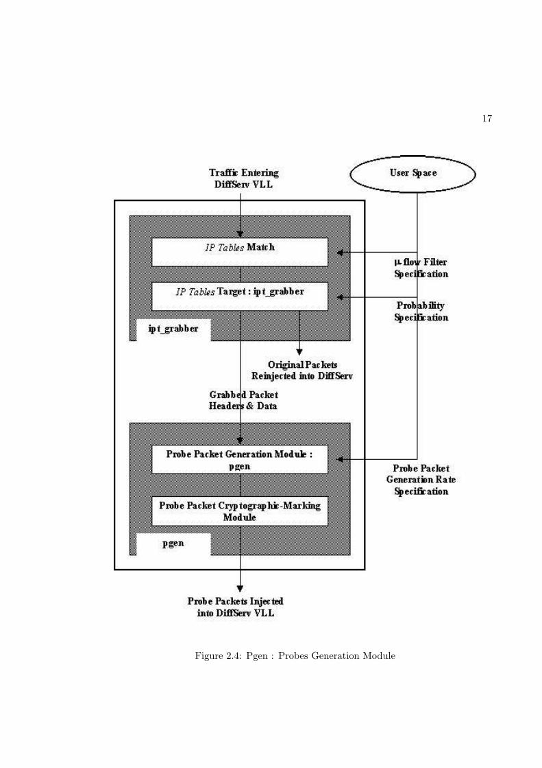
• PGen : The stealth Probe Packet Generation module is placed on the boundary
routers of the VLL to be monitored. As illustrated in Figure 2.4, PGen periodically
makes a copy of a random packet from the VLL inward-flow, marks the new copy
with a stealth cryptographic hash and reinjects both the packets into the VLL. If
a packet is not available in the VLL to be copied and reinjected, a new packet is
still injected though with the contents of the packet last copied. The injection of
probes is done in a soft real time manner at a low specified rate. The idea is to
generate a strictly stationary flow with a fixed and known packet rate and zero jitter
before entering the DiffServ cloud. The QoS parameters that are monitored for this
flow then are highly predictable. Deviations from these stationary means are then
a function of the DiffServ cloud. PGen also appends the hash with an encrypted
sequence number for the probe packet that is necessary for jitter calculation at the
egress router. It is built inside the Linux kernel as a loadable module. It operates in
tandem with the iptgrabber kernel module. Once loaded, the latter copies the entire
content of randomly chosen packets matching a certain filter criterion into a kernel
memory buffer. It runs as a target module of a IP Tables[11] match. The match is
specified through command line arguments to the iptables user space tool. We set
the match to select only the VLL packets. The rate or chance of packet capture is
specified through the kernel’s proc filesystem.
For our tests, we have used unencrypted hashs and sequence numbers on the probes.
In practice, we would use a secure hash to tag the packets based on a shared secret
17
Figure 2.4: Pgen : Probes Generation Module

18
key between the boundary routers of the VLL and certain field(s) in the IP packets.
The idea being that, then, the attacker would not be able to, with a significant level of
certainty, distinguish between probe packets and the normal data packets. The use of
IPSec with data encryption over the VLL clearly helps this requirement. The probes
are terminated at the egress router. Interior routers simply forward packets and do
not expend any processing effort on an encryption or decryption process.
Then, all attacks on the QoS of the VLL are statistically spread over both the normal
data and the probe packets. We assume that such a secure probe tagging or marking
method can be implemented effectively, however, we do not research this area any
further in this work. In this respect, the secrecy of this mark should be considered as
a single point of failure for ArQoS security for that VLL.
For jitter and delay parameters, we need monitor only the low volume probe flow.
The rate of probe generation can be considered negligible compared to the rate of
the VLL flow. Typical rates are 1 or 2 probe packets in a second. Large rates would
have flooded the network unnecessarily while lower rates would require unacceptably
longer time windows over which to generate the short term profiles, that is, a sluggish
detection rate. This sluggish detection rate due to low logging sampling frequencies
is a corollary to the procedure used to statistically profile and then compare the short
and long term behaviors of the flow parameters, and is described both quantitatively
and qualitatively in the following two chapters.
• TrafMon and PgenMon : Figure 2.5 illustrates the architecture of TrafMon and Pgen-Mon micro-flow monitors. TrafMon monitors arbitrary flows non-invasively and in-
dependently of the probes. PgenMon monitors only the probes sent by Pgen at the
other end of the VLL. Both are placed on one of the boundary routers of VLLs that
they monitor. We use TrafMon to monitor only the bit rates of (approximately or
close to) Constant Bit Rate (CBR) flows. We use PgenMon to monitor the jitter,
and the packet rates of the probe flow inside a VLL. These use the libpcap library to
specify microflows to filter and monitor statistics for. Libpcap in turn uses the Linux
Socket Filter inside the Linux kernel. All the filtering therefore takes place inside the
kernel which is necessary to avoid missing packets when the flow arrives at high rates.
Both monitors are multithreaded, in that they can monitor more than one microflows
on the same router. The exact flows to monitor, the local or remote NIDES/STAT

19
Figure 2.5: Pgen mon and Traf mon : Probe and Micro-Flow Monitor
and RULE modules to send the statistics to, the frequency of sampling the measures
and of sending are all user specifiable.
Thus far, we have seen the motivation for QoS anomaly detection, an overview
and an elaboration of the QoS monitoring sensors, their placement on the DiffServ domain
and the coordination between them. With this overview of the detection components and
QoS domain configuration, the following two chapters detail the procedure used for and the
mathematical background of the statistical anomaly detection (chapter 3) and the statistical

20
process control (chapter 4) approaches.

21
Chapter 3
Statistical Anomaly Detection
3.1 The Concept
Statistical Anomaly Detection is based on the hypothesis that a system being
monitored for intrusions will behave anomalously when attacked and that these anomalies
can be detected. The approach was first introduced in [7]. [9] compares it with other
intrusion detection approaches.
Thus far, we have used the acronym NIDES/STAT to refer to both the present sta-
tistical anomaly detection engine/algorithm and the EWMA SPC Chart-based engine/technique.
For this and the next chapters, and throughout the thesis, wherever they are compared
against each other, we use NIDES/STAT to refer to only the anomaly detection algorithm
and EWMA to refer to only the EWMA SPC Chart-based approach. The approach referred
to would be apparent from the context of the discussion.
In general, a statistical anomaly detection system continuously samples specific
parameters of a system. It also continuously generates two types of statistical profiles of
these parameters. The first type estimates the average of the values of the parameters over a
long enough duration of time. By doing this, by definition of statistical estimation, it can be
expected that the future samples of the individual parameters will be centered around their
respective profile estimates. The second type of profile estimates the average of the values
sampled over a relatively shorter period of time and only in the recent past. Extending the
above argument, then, it is expected that the short term profile will be within a statistically
close range of the long term profile unless the underlying base stochastic process itself has
shifted (in mean, variance etc) over this recent past.

22
For our anomaly detection approach, NIDES/STAT, the profile referred to in
long term and short term profiles is a Probability Density Function (PDF) of the monitored
statistic. In view of this then, a long term profile is essentially the PDF exhibited by or
observed for the statistic, in the long term period of observation of its outcomes/samples.
Similarly, the short term profile is the PDF exhibited by the statistic for the recent past.
For this work, we define a statistically predictable system as one in which
the long term profile of the stochastic process/system, measured by NIDES/STAT as de-
fined above, does not change significantly in the time over which the short term profile
is measured. As a necessary (but not sufficient) condition then, the generating moments,
especially the mean and the variance, of such processes/systems do not shift significantly
over the recent past as well. These are similar in spirit to the random processes that are
stationary up to order 2 - the ones which have means and variances that do not vary over
time. Whereas a strictly stationary process thats stationary up to order 2, severely restricts
an evolution of the first and the second generating moments of the process over time, a
statistically predictable system only requires (reiterating, not suffices with) that the gen-
erating moments not change significantly over the recent past period over which the short
term profile is calculated. Consequently, a predictable system does allow for gradual shifts
in the mean and variance of the underlying base process over large multiples of the short
term period. We hypothesize that for statistically predictable systems, a significant devia-
tion of the short term profile from the long term profile is an anomaly. This is the rationale
behind the statistical anomaly detection approach, NIDES/STAT.
3.2 Justification for using the NIDES
The Statistical Anomaly Detection approach has faced severe criticism from the
intrusion detection community due mostly to its high false alarm generation rate[24]. How-
ever, the effectiveness of this approach in fact depends on the nature of the subject to a
large extent.
Statistical anomaly detection is, in general, well suited for monitoring subjects
that have a sharply defined and restricted behavior with a substantial difference between
intrusive and normal behavior. A QoS flow is an ideal candidate for such a subject and
justifies the use of anomaly detection for monitoring it.
The statistical anomaly detection algorithm we use, NIDES/STAT, is based on

23
SRI’s NIDES[19] algorithm. This algorithm was originally applied to subjects which were
users using a computer’s operating system and associated software utilities on it. It is
impossible to accurately profile a statistically unpredictable system without making as-
sumptions on the system’s behavior that are only theoretically interesting. As reasoned
below, a user on a computer system and the operating system itself are unpredictable sub-
jects, that can not be profiled, and are hence unsuitable for statistical anomaly detection.
With that in perspective, below is a justification of why the NIDES/STAT algorithm is
suitable for monitoring the network QoS.
• NIDES/STAT monitors statistically predictable subjects only. The subjects of interestspecific to this work are the QoS statistics, namely, byte rate, packet rate, jitter and
end-to-end delays of the QoS flow packets. Flows sensitive to network QoS (such
as VoIP or RealAudio audio or MPEG4 video streams) typically differ from flows
that can manage with only a best-effort network service (such as web traffic, email
traffic etc) in that the former are by design much more predictable with (most of)
these QoS statistics. A reasonable SLA that makes QoS guarantees can only be
written for flows that show such a reasonable predictability. For example, a packet
forwarding assurance of 99.95% ( no more than 5 packets be dropped in 10000 packets)
for a 128kbps Committed Information Rate (CIR) can not be reasonably made for
a flow that switches rates to 256kbps under heavy user loads. A TCA (between the
ISP network and the customer network) is then designed to enforce this reasonable
predictability in the QoS flow, so that the SLA can be applied to it. A TCA dictates
the behavior of the incoming QoS flow parameters for suitability towards the SLA and
penalizes the out-of-profile flows and packets through pre-determined actions explicitly
stated in the TCA. For example, an ISP could use a 128kbps CIR, 20KB Committed
Burst Size (CBS) Token Bucket Filter (TBF) at its ingress node to police the incoming
QoS flow and mark (say) all the out-of-profile packets to be dropped or given only
best-effort service etc. (A detailed discussion of TBF policing can be found in [42]).
A critical assumption that this thesis is based on is that the network’s status or QoS
as experienced by a QoS flow in the absence of attacks in terms of parameters like the
propagation or routing delay and delay variation, drop or error rate, congestion level,
packet duplication rate etc is a statistically deterministic or predictable process. This
becomes intuitively clear and reasonable knowing that in a DiffServ domain, the flows

24
already present in the network are protected by traffic admission control and policing
at the ingress routers and also by the relatively differentiated services that flows of
different priority classes experience. DiffServ SLAs and TCAs ensure that the QoS is
as specified and hence predictable (in the absence of attacks). An important point to
note in this context is that a failure to do so will also be considered as an anomaly
and detected, irrespective of whether the network QoS was attacked externally or not.
NIDES/STAT is carefully used only for QoS statistics that are predictable. Thus,
for example, if a QoS flow has predictable and well bounded or defined byte rate,
packet rate and end-to-end delays but unpredictable jitter, then NIDES/STAT does
not monitor the jitter for such a flow. Jitter can still be monitored for that VLL by
injecting probes into it. Since the probes are sourced deterministically (periodically)
into the DiffServ cloud, the jitter at the egress router is a function of the DiffServ
cloud only.
• In general, a statistical anomaly detection system monitoring a user or operating sys-tem usage can be evaded easily. Once the detection algorithms are published, an
attacker who is an intelligent agent and not a random statistical process can evade
detection by effecting undetectable intrusive actions that have undetectable effects.
The actions can be undetectable by virtue of their type being beyond what is moni-
tored, their time distribution or sequence, interleaving with other harmless ones and
other common measures of deception. The effects being monitored are known and a
skilled attacker will avoid actions that have detectable effects. Security of a computer
system involves prevention of unauthorized reading, deletion or modification of data,
unauthorized system usage, connections to and from other systems etc. Most/all of
these, typically, do not have easily detectable effects. Hence IDSs on computer systems
have to detect intrusive actions in addition to, if at all, effects on system behavior.
In contrast to this, NIDES/STAT can not be evaded easily. NIDES/STAT monitors
only the effect of attacks and not the attacks themselves. Since the effects monitored
are the ones on parameters that are also a part of the SLA and the TCA, an un-
detectable effect of an attack signifies no disruption of the QoS. In other words, the
attack is then not violating the SLA/TCA that define the QoS requirements. The
attack then is insignificant as far as QoS provisioning is concerned. A critical as-
sumption on which this is based is that the routers (ingress and egress) that do the

25
metering and monitoring for the SLA/TCA are not compromised. We have already
justified the reasonability of this assumption in section 2.2.
• The network traffic including the probes do not have any particular distribution andinstead have distributions that are specific to the network and its status. The NIDES
algorithm that NIDES/STAT uses also does not assumes any specific distribution or
model for the subject. The only requirement NIDES asks of the distribution is that
it be fixed or slow moving, meaning the profiled process be statistically predictable.
As argued before, this is a reasonable assumption for NIDES/STAT when applied to
QoS flow parameters.
With this justification and motivation for the use of NIDES/STAT for QoS moni-
toring in mind, we now look at the mathematical background for NIDES/STAT.
3.3 Mathematical Background of NIDES/STAT
3.3.1 The χ2 Test
The statistical anomaly detection is done by the NIDES/STAT module in com-
bination with a EWMA Statistical Process Control module that monitors only highly sta-
tionary processes with very low deviations (for reasons described later in this chapter). The
NIDES/STAT module is treated here and the latter in the following chapter 4.
For a random variable, let E1, E2, ..., Ek represent some k arbitrarily defined,
mutually exclusive and exhaustive events associated with its outcome and let S be the
sample space. Let p1, p2, ..., pk be the long-term or expected probabilities associated with
these events. That is, in N Bernoulli trials, we expect the events to occur Np1, Np2, ...,
Npk times as N becomes infinitely large. For sufficiently large N, let Y1, Y2, ..., Yk be the
actual number of outcomes of these events in a certain experiment. Pearson[31, 15] has
proved that the random variable Q defined as
Q =k
∑
i=1
(Yi −Npi)2
Npi(3.1)
has (approximately) a χ2 distributed Probability Density Function with k -1 degrees of
freedom if any k -1 of the events are independent of each other. The approximation is good
if Npi ≥ 5, ∀i so that no one event has so large a Qi component that it dominates over the

26
rest of the smaller ones. Rare events that do not satisfy this criterion individually may be
combined so that their union may.
The pi are the long term probability distribution of the events. Let p′i =YiN be
the short term (meaning the sample size, N, is relatively small) probability distribution of
the events.
Our test hypothesis, H0, is that the actual short term distribution is the same as
the expected long term distribution of the events. Its complement, H1, is that the short
term distribution differs from the long term one for at least one event. That is,
H0 : p′i = pi, ∀i = 1, 2, ..., k and H1 : ∃i, p′i 6= pi
Since, even intuitively, Q is a measure of the anomalous difference between the
actual and the expected distributions, we expect low Q values to favor H0 and high Q
values to favor H1.
Figure 3.1: χ2 Statistical Inference Test

27
As Figure 3.1 indicates, we define α as the desired significance level of the hy-
pothesis test. Also, let χ2α(k-1) be the corresponding value of Q, that is, such that,
Prob(Q ≥ χ2α(k − 1)) = α. For an instance of Q, say qk−1, we reject the hypothesis
H0 and accept H1 if qk−1 ≥ χ2α(k − 1).
So, with every experiment, we make N Bernoulli trials and calculate a Q based
on Equation 3.1. Based on the above inequality criterion then, we determine whether, or
more precisely, assume that Q and therefore the experiment was anomalous or as expected
(normal).
Qualitatively, α is a sensitivity-to-variations parameter; the lower we set the value
of alpha, the lesser would be the rate at which even relatively large and rare Q’s will be
flagged anomalous, while the higher we set it, the higher will be rate at which even relatively
lower and usual Q values will be declared anomalous.
3.3.2 χ2 Test applied to NIDES/STAT
In the context of NIDES/STAT, the random variable sampled is the measured
count of a QoS parameter of the network flow being monitored. The experiment is the
process of measurement or sampling of the parameter’s value. As will be seen soon, we
do not sample the parameter multiple times (the N trials from above), but rather with
each sample (the experiment), we use an exponentially weighted moving average process to
estimate the parameter’s most recent past (short term) profile. In view of this, N takes a
new form Nr that’s described later in this chapter.
The QoS parameters we use presently are
• Byte Count is the number of bytes of the network flow data that have flowed in afixed given time (from the last logging time to the present one). The rationale behind
this parameter is that QoS flow sources tend to be fairly CBR or low-deviation VBR
sources. As mentioned before, this is due to encoder or fixed-bandwidth channel
compatibility related design issues. For example, [6] illustrates the observed CBR-
like property exhibited by RealAudio sources when observed at 10s of seconds of
granularity which is absent at lower (¡10s) granularities.
• Packet Count is the number of probe packets of the network flow data that have flowedin a fixed given time. Packet count is used only for probe packets to measure traffic
rate independent of packet size.

28
• End-to-end Delay is the total delay experienced by the network flow packets from theingress to the egress of the VLL of the DiffServ cloud. Due to practical difficulties
and issues with time-synchronization of the boundary nodes, we limit the use of this
measure only for the tests with simulations.
• Jitter is defined as the average (of the absolute values of the) difference between theinter-arrival times of consecutive probe packet pairs arriving at the egress router of a
VLL. The calculation makes use of the sequence numbers that the probe packets carry
to identify the order in which the packets were actually injected into the system. For
CBR sources, like the probes, using inter-arrival time jitter eliminates the need for
end-to-end delay jitter. For VBR sources, to measure end-to-end delay, in general, we
would need to time stamp packets at the ingress and to time synchronize the boundary
routers. We focus on inter-arrival time jitter for probes only in this work.
NIDES/STAT can be extended to use other measures that matter to the SLA.
NIDES/STAT is trained with the maxima and the minima of every parameter. This range
is linearly divided into several equal-width (equal interval size) bins into which the count
outcomes may fall. These are the events used by the χ2 Test. The number of bins is
arbitrarily set at 32. Hence, any 31 events out of the total 32 events are independent. Thus
we expect a χ2 Distribution for Q the maximum degrees of freedom of which are 31.
Sections 3.3.3 and 3.3.4 detail how the long term and the short term distributions
of the counts are obtained.
NIDES/STAT algorithm defines a variable S to normalize the values of Q from
different measures and/or flows so that they may be compared against each other for alarm
intensities. This is done such that S has a half-normal probability distribution satisfying
Prob(Sε[s,∞)) = Prob(Q > q)
2
That is,
S = Φ−1(1− Prob(Q > q)
2) (3.2)
where Φ is the cumulative probability distribution of the Normal N(0, 1) variable. This
ensures that S varies from 0 to ∞, but we limit the maximum value of S to 4 since thatand higher values are rare enough to be considered a certain anomaly.

29
3.3.3 Obtaining Long Term Profile pi
To establish the long term distribution for a measure, the detection system is first
placed on the QoS domain when it has been absolutely isolated from any malicious attacks
on its QoS flows (for example, when the SLAs are met and the QoS on manual inspection
is as expected). NIDES/STAT is then trained with the normal (that is, unattacked) QoS
flow statistics. Once it learns these training measures, it has a normal profile against
which to compare a recent past short term profile for anomaly detection. The phases that
NIDES/STAT goes through while building a long term normal profile are -
1. Count Training : where NIDES/STAT learns the count maxima, minima, mean and
the standard deviation over a specified, sufficiently large, number of training measures.
The maxima and the minima help in the linear equi-width binning used by the χ2
Test.
2. Long Term Training : At the end of a set number of long-term training measures,
NIDES/STAT initializes the pi and the p′i equal simply to the bin frequencies as
pi = p′i =CurrentCountiCurrentTotal
(3.3)
where CurrentCounti is the current number of ith-bin events and CurrentTotal is
the current total number of events from all the bins.
These are the initial long term and short term distributions.
3. Normal/Update Phase : After every preset Long Term Update Period, NIDES/STAT
learns about any changes to the long term distribution itself. By using exponentially
weighted moving averages, the older components in the average get exponentially de-
creasing significance with every update. This is important since the flow parameters,
though typically approximately stationary in a QoS network, may shift in mean over
the long update period and this shift needs to be accounted for to avoid false positives.
This is done as
LastWTotal =WTotal (3.4)
WTotal = b× LastWTotal + CurrentTotal (3.5)

30
and
pi =b× pi × LastWTotal + CurrentCounti
WTotal(3.6)
Here, b is defined as the weight decay rate at which, at the end of a preset LTPeriod
period (long term profiling period) of time, the present estimates of CurrentCounti
and CurrentTotal have just a 10% weight. Typically, LTPeriod is about 4 hours
(as justified in chapter 6). Clearly, equation (3.6) then gives the required long term
frequencies pi as the ratio of the EWMA of the current bin count to the EWMA of
the current total count. Further, only the most recent LTPeriod period has a (90%)
significance to the long term profile.
3.3.4 Obtaining Short Term Profile p′i
Unlike the long term frequencies pi, the short term ones are updated with every
count as
p′i = r × p′i + 1− r (3.7)
and
p′j = r × p′j , ∀j 6= i (3.8)
where i is the bin in which the present count falls. r is the decay rate, defined
in NIDES/STAT as the rate at which the current short term bin frequency estimate has
a weight of 1% at the end of a STPeriod period (short term estimation period) of time.
STPeriod is about 15 minutes (as justified in chapter 6). The 1 − r in the equation (3.7)
satisfies∑
p′i = 1 and also serves as the weight for the present count of 1 for the bin to
which the present measure belongs. Further, only the most recent STPeriod period has a
(99%) significance to the short term profile.
3.3.5 Generate Q Distribution
The calculation of the Q measure in NIDES/STAT is based on but a slightly
modified version of Equation 3.1. Since the short term profile p′i are calculated through an
EWMA process as described above in Equations 3.7 and 3.8, wherein, the previous estimate
is given a weight of r, NIDES/STAT is careful in its use of N , the number of samples used

31
to build the short term profile. We define Nr as the effective sample size based on the
EWMA process given by
Nr = 1 + r + r2 + r3 + ... ≈ 1
1− r(3.9)
which makes Equation 3.1 as
Q =32∑
i=1
(p′i − pi)2
pi
Nr
(3.10)
NIDES/STAT maintains a long term Q distribution curve, against which each new
short term Q is compared to calculate the anomaly score S. The long term Q distribution
generation is very similar to the long term frequency pi distribution generation. The pro-
cedure parallels the one in section 3.3.3, where equations (3.3) through (3.6) now become
-
at the end of a specified long term training Q measures, we set
Qi =CurrentQCountiCurrentQTotal
(3.11)
where we arbitrarily use a 32 bin equi-width partitioning, CurrentQCounti is the
current number of ith-bin Q events and CurrentQTotal is the current total number of Q
events from all the bins.
Further, in the update/normal phase, after every long term update Q measures,
we use
LastWQTotal =WQTotal (3.12)
WQTotal = b× LastWQTotal + CurrentQTotal (3.13)
and
Qi =b×Qi × LastWQTotal + CurrentQCounti
WQTotal(3.14)
to get the long term Q distribution.
3.3.6 Calculate Anomaly Score and Alert Level
As mentioned before in section 3.3.1, α serves as a parameter to specify the required
sensitivity to variations in Q. In an anomaly or attack detection context, then, α refers to
the False Positive Rate (FPR) specification. A lower α flags as anomalies only exceptionally

32
large Qs that are consequently rare. This means both that, 1. in the absence of attacks,
the False Alarms or False Positives are generated only rarely (low FPR), while 2. in the
presence of attacks, only severe ones that generate exceptionally high Qs will be detected
(low detection rate). αs are then set to strike a tradeoff between the required false positive
and detection rates. Multiple αs can be used to classify different levels of attacks in terms
of severity and likelihood.
Equation (3.2) gives the degree of anomaly associated with a new or short term
generated value of Q, say q. This S score also determines the level of alert based on the
following categories -
• Red Alarm Level - S falls in a range that corresponds to a Q tail probability of
α = 0.001. This means that Q’s and S’s chances of having such high a value are 1 in
a 1000. (High severity, Low likelihood)
• Yellow Alarm Level - S falls in a range that corresponds to a Q tail probability of
α = 0.01 and outside the Red Alarm Level range. Then, Q’s and S’s chances of falling
in this tail area are roughly 1 in a 100. (Medium severity, Medium likelihood)
• Normal Alarm Level - For all values of S below the Yellow Alarm Level, we generatea Normal Alarm that signifies an absence of attacks. (Normal level, Usual)
If after an attack is detected, it is not eliminated within the LTPeriod period
of time, NIDES/STAT learns this anomalous behavior as normal and eventually stops
generating the attack alerts.
Certain parameters such as the drop rate associated with an AF probe flow in
an uncongested network may be highly stationary with zero or very low deviations. For
such parameters, the long term frequency distribution pi does not satisfy the Npi > 5 rule
for all expect possibly one or two bins. The χ2 test does not gives good results for such
parameters. NIDES/STAT does make an attempt to aggregate rare bins which do not
satisfy this criterion into a single event that does (due to increased bin frequency). We
find, however, that whenever the number of Qi components calculated satisfying the above
rule-of-thumb (the rare aggregated group of bins counting as one component) falls below 3,
the performance of NIDES/STAT in terms of its Q profile generation, detection and false
positive rates degrades significantly. Hence, as a rule of thumb, whenever the number of
such Qi components for any sample falls below 3, we use the EWMA Control Chart mode

33
for finding the anomaly score. When it exceeds or equals 3, we switch back to the χ2 mode.
In simpler words, for QoS statistics with extremely low-deviation long term distributions,
which do pose this problem, we switch to EWMA Control Chart mode to generate anomaly
scores.
The next chapter describes the EWMA Statistical Process Control Chart approach.
34
Chapter 4
EWMA Statistical Process Control
The Exponentially Weighted Moving Average (EWMA) Control Chart is a popular
Statistical Process Control technique used in the manufacturing industry for product quality
control. In this, a probability distribution curve for a statistic gives the rarity of occurrence
of a particular instance of it. Outcomes that are rarer than a certain predefined threshold
level are considered as anomalies. As explained, the NIDES/STAT algorithm is not suitable
for a highly stationary measure with very low deviations, and it is for only such measures
that we use the EWMA Control Charts to detect intrusions.
For example, a QoS customer network could be sourcing a relatively unpredictable
VBR flow with mean packet and byte rates shifting swiftly over time, and could reserve a
QoS bandwidth to accommodate even the highest rates it generates (over provision). The
flow itself might be very sensitive to packet dropping and would reserve an AF (Assured
Forwarding with low drop precedence) QoS class from the DiffServ ISP for that. The ISP
would then use probes to monitor the packet rates, since the flow’s corresponding statistic
is not suited for anomaly detection. Due to the use of AF class and over provisioning
though, the flow could receive exceptionally low packet drop rates. In this case then, the
statistic produces an exceptionally stationary (since probes are inserted into the VLL at a
fixed soft real-time rate) distribution with a deviation too low for NIDES/STAT to profile
or handle using the χ2 test. However, due exactly to this exceptionally high predictability,
the statistic is well suited for the EWMA Statistical Process Control technique.
We believe this is the first work to suggest using EWMA Statistical Process Con-
trol Charts for Intrusion Detection. Reiterating, the technique is only useful for highly
predictable and restricted subjects (as in the example above) and attempts to use it on

35
arbitrary subjects will lead to excessive false alarms.
4.1 Statistical Process/Quality Control
Shewhart[38, 39, 37] first suggested the use of Control Charts in the manufacturing
industry to determine whether a manufacturing process or the quality of a manufactured
product is in statistical control. The EWMA Control Charts, an extension of the Shewhart
Control Charts, are due to Roberts[34].
In EWMA Control Charts, the general idea is to plot the statistic εk given as
εk = λxk + (1− λ)εk−1 (4.1)
Here, a subgroup of samples consists of n independent readings of the parameter of interest
(from n different manufactured products at any instant of time). Samples are taken at
regular intervals in time. Then, xk is the average of the kth subgroup sample. λ is the
weight given to this subgroup average. εk is the estimator for this subgroup average at kth
sample. The iterations begin with ε0 = x. x is the (estimate of the) actual process mean,
while σ̂ is the (estimate of the) actual process standard deviation.
If λ ≥ 0.02, as is typical, once k ≥ 5, the process Control Limits can be defined as
x± 3 σ̂√n
√
λ
2− λ(4.2)
Let UCL denote the upper control limit and LCL denote the lower control limit,
STE denote the short term estimate and LTE denote the long term estimate. For a base
process that is Normally distributed, the STE estimator then falls outside the control limits
less than 1% of times.
Ignoring the first few estimates then, when the iterations stabilize, we consider any
estimate outside the control limits as an anomaly. The cause of the anomaly is then looked
for and if possible eliminated. If the fault(s) is not corrected, the control chart eventually
accepts it as an internal agent.
The EWMA estimation is essentially a simple (order 1) Low-pass Infinite Impulse
Response (IIR) filter; the sampling interval is the time between two readings or samples of
the statistic xk, the co-efficient λ determines the cut-off frequency.

36
In case of samples that do not involve subgroups, that is, where n = 1, the equa-
tions (4.1) and (4.2) become
εk = λxk + (1− λ)εk−1 (4.3)
and
x± 3σ√
λ
2− λ(4.4)
where we begin with ε0 = x.
It is important to note that the X chart (based on subgrouping) is more sensitive
in detecting mean shifts than the X chart[36] (based on individual measures). Hence,
wherever possible the X chart should be preferred.
The value of the EWMA weight parameter λ is chosen as a tradeoff between
the required sensitivity of the chart towards fault detection and the false positive rate
statistically inherent in the method. A low λ favors a low false positive rate, whereas a
large value favors high sensitivity. Typically, in industrial process control, it is set at 0.3.
Figure 4.1 shows an EWMA SPC Chart for a statistic with a Normal distribution. It is
interesting to note how closely the Control Limits LCL and UCL follow the short term
estimate STE while still allowing enough variability to it; out of the 4000 samples shown,
only 2 generate process out-of-control alerts by falling beyond the control limits.
165
170
175
180
185
190
195
05001000150020002500300035004000
EW
MA
Sta
tistic
Val
ues
Log Number (tens of seconds before present)
LCLSTEUCLLTE
Figure 4.1: EWMA SQC chart for a Normal process

37
4.2 Application to Network Flows
In ArQoS, we consider the QoS flows/flow-statistics as quality controlled processes
where the quality parameters of interest are the bit rates, packet drop rates, end-to-end one-
way or two-way delays, and jitter of the flows.
A significant difference between the requirements of NIDES/STAT and EWMA is
that NIDES/STAT requires a suitable subject statistic to have an approximately stationary
long term distribution (all generating moments be approximately stationary), while EWMA
requires only that the first generating moment, that is the mean, be approximately station-
ary (and that the variance be low). Thus, a subject statistic suitable for NIDES/STAT is
suitable for EWMA if it has a low variance.
In statistical process control, the EWMA control chart is used to detect small shifts
in the mean of a process to indicate an out-of-control condition. In contrast, in ArQoS, we
monitor flow processes that are only required to be weakly stationary, and hence have to
allow for a gradual shift in their means over sufficiently long periods of time. However, a
swift shift will be detected as an anomaly and flagged.
In view of the above, an actual process mean x, which we represent as LTE, is
found as an exponentially weighted moving average as
LTEk = (1− rLT )LTEk−1 + rLTxk (4.5)
where the decay parameter rLT makes LTE significant only for the past LTPeriod period
in time, just as with NIDES/STAT. The flow processes are chosen such that the mean does
not shift significantly over this period of time. Any small shift is reflected as a shift in LTE.
Similarly, the long term count square, LTCntSq is found as
LTCntSqk = (1− rLT )LTCntSqk−1 + rLTx2k (4.6)
and the long term standard deviation, σ̂ or LTStdDev is found as
LTStdDev =√
LTCntSq − LTE2 (4.7)
The EWMA statistic εk, which we represent by our short term estimate parameter
STEk, is given by
STEk = rSTEk−1 + (1− r)xk (4.8)

38
where the decay rate r is the same as the short term decay parameter used in NIDES/STAT.
The STE estimate has STPeriod as the moving window of significance.
Then, the equation (4.2) gives the EWMA control limits as
LTE ± 3LTStdDev√n
√
1− r
1 + r(4.9)
where n equals 1 for byte and packet counts, but is greater than 1 for parameters like jitter
and end-to-end delay measures that are averaged over several packets.
STEk, LTEk, LTCntSqk and the control limits UCLk and LCLk are calculated
for every received measure and an alarm is raised whenever STEk falls beyond either of the
control limits. The EWMA control chart mode generates only Normal and Red Alarms.
Although the QoS parameters of interest to us are strictly not Normally dis-
tributed, nevertheless, our results indicate that the fairly stationary and low-deviation
parameters we study do fall beyond the control limits only under anomalous conditions,
that is, when under attack.
We have in the present and previous chapters described the motivation for the
detection system, the architecture of its detection engine and sensor components, the coor-
dination between these and the mathematical basis of the detection algorithm. In the next
chapter we describe the emulation and simulation experiments we do to test and validate
these components and the detection algorithms.

39
Chapter 5
Experiments with Attacks and
Detection
This chapter describes our experiments with the attacks and the detection system.
We run two sets of experiments. One set involves an actual emulation of the DiffServ
domain on a network testbed, with kernel and user space modules to generate best-effort
and QoS flows, to sample QoS flow parameters, to effect the attacks, etc. The second set of
experiments involves a thorough validation of the emulation tests using a network simulator
to simulate the DiffServ domain, the various background and QoS flows, the attacks etc.
Due to implementation issues, we test almost the same set of attacks on both the
simulation and the emulation experiments, except that with the simulations, we do not test
for jitter attacks and with the emulation, we do not test for end-to-end delay attacks, and
intermittent/bursty attacks. It is important to note that detection of attacks on end-to-end
delay requires that the boundary routers be time-synchronized with each other, which is a
fairly significant challenge. Any such implementation could have other security weaknesses
like attacks on packets containing time synchronization information. We make no attempt
to time-synchronize the boundary nodes in our emulation tests and thereby do not test for
this particular attack in those.
These experiments are used to test the attack detection capabilities of NIDES/STAT,
EWMA Charts and RULE under varying intensities of attacks, on different QoS parameters,
when attacks are persistent or when they are applied in intermittent bursts. The attack
detection capabilities include the detection rate, detection time and false positive rates.

40
The results and observations from these tests are summarized in the following chapter.
5.1 Tests to Validate Algorithms
To verify the correctness of the NIDES/STAT and the EWMA Control Chart
algorithms, we use simulated normal network traffic and simulated attacks. With an in-
dependent computer code (without any consideration about network topologies or effects
thereof), we generate independent values for a random variable that has an arbitrary but
stationary distribution (fixed mean and variance). This random variable represents any of
the various QoS parameters we intend to monitor in practice. Example distributions we use
include Normal, Uniform, and other bell-shaped arbitrary distributions with known means
and variances that are kept fixed. These series of random variable outcomes or values then
represent the normal, that is, unattacked, QoS parameter values. The NIDES/STAT, and
EWMA Charts are trained with these values over a significant sample size to represent
the long term period. Then, 1. the long term distribution generated by NIDES/STAT
should match (at least approximately) the (equi-width binning distribution of the) original
distribution of the statistic (Normal, Uniform etc). This validates the binning and EWMA
estimation process used by NIDES/STAT. 2. The Q distribution generated should approx-
imately follow a χ2 distribution with k − 1 degrees of freedom (from Equation 3.1), wherek is determined from the original distribution’s equi-width binning and finding the number
of bins that satisfy the rule-of-thumb Npi ≥ 5 including the rare-bins groups, if any. Thisvalidates the Q measure generation algorithm in NIDES/STAT. 3. The rate of false posi-
tive generation should be approximately 1% for EWMA Charts and the Yellow alerts from
NIDES/STAT and about 0.1% from the Red alerts from NIDES/STAT. We then test the
false alarm and detection rates by varying the base process’ mean and variance (separately)
first gradually over a large sample size (to represent a gradual and normal change in the
QoS flow behavior), and second by doing this quickly over a short sample size (to repre-
sent attacks of moderate to high intensities). The detection system should be expected to
generate minimal alarms for the former, while flagging anomalies for the latter.

41
5.2 DiffServ Domain and Attacks : Emulation Experiments
5.2.1 DiffServ Network Topology Setup
VLL
RealPlayerRTSP/TCP
Probes
TCP/UDP(BE)
PGenArQoS IDS
RealServer
��������
������
�� ����
��������
�����
����
�����
����
�����
����
�����
����
!!!!
Figure 5.1: Network Setup for Tests
Figure 5.1 shows a condensed topology for our isolated DiffServ capable network
testbed. All the routers we use are Linux kernels configured with DiffServ capabilities. For
this, we use the traffic conditioning configuration utility tc that comes with iproute2[22] to
configure the queueing disciplines, classes, filters and policers attached to the kernel network
devices.
5.2.2 QoS-Application Traffic Setup
We setup a VLL between an ingress and an egress router. It is setup using only IP
address based routing entries and DSCP based service class mappings. The VLL, sourced
and sinked by a RealVideo client-server pair as shown, carries an audio-video stream that
uses Real Time Streaming Protocol (RTSP) for real-time signalling, and either EF or AF
(in separate tests) as the DiffServ class type for minimal delay or minimal drop rates in
forwarding.
5.2.3 Background Traffic Setup
We use MGEN/DREC[1] to generate a Poisson distributed UDP BE background
traffic. thttp[8] generates a HTTP/TCP BE background traffic based on an empirical HTTP
traffic model[25]. The idea is that it is easier to observe the relatively differentiated for-

42
warding services in a moderately or heavily flooded network. Further, it is more interesting
to attempt to distinguish effects on the QoS due to attacks from those due to random fluc-
tuations in the background traffic. The combination of the Poisson and the HTTP models
attempts to capture the burstiness (due to the HTTP model), and the randomness (due to
both models) typical to the aggregate Internet traffic. We do acknowledge that this model
is not entirely representative of the Internet traffic, and use a much better traffic model
with the simulation experiments. To emulate a Wide Area Network (WAN), we introduce
end-to-end delays and jitter in each of the routers using NISTNet[5]. We use round-trip
delays with means of the order of tens of milliseconds and standard deviations of the order
of a few milliseconds to emulate a moderate sized DiffServ WAN with low congestion.
5.2.4 Sensors Setup
Probes are generated at the ingress side of the video (data) flow and the PgenMon
and TrafMon sensors, along with the detection engine components are placed on the egress
router. We configure the video stream server to stream a Variable Bit Rate traffic (VBR)
with a fixed mean rate and low deviation within the congestion that the VLL normally
experiences. PgenMon monitors the jitter and the packet rate of the probes, whereas
TrafMon monitors the bit rate of the video streaming (one-way) flow.
5.2.5 Attacks Setup
For the attacking agents, we again use NISTNet to significantly increase the end-
to-end delays and the jitter in the QoS flows. (We test for end-to-end delay attacks only in
the simulation experiments, and for the jitter attacks only in the emulation experiments.)
We also use Linux kernel modules, we call ipt drop and ipt setTOS, as the packet dropping
and packet remarking modules respectively. These are based on the IPTables’[11] packet
capturing and mangling framework. The modules are written as IPTables’ kernel extensions
to be called whenever a predefined filter independently captures a packet.
Thus, based on a specified filter, a selected flow can be subjected to any combi-
nation of packet dropping, packet DSCP-field remarking, and introducing extra jitter and
end-to-end delay variation attacks. The attack intensities are user configurable.
NIDES/STAT and the EWMA chart module are trained with the VLL and the
probe flows in the absence of any attacks, and RULE is configured for checking conformity

43
with the SLA. Then the individual attacks are launched to check the detection capabilities
of the modules. It is important to note that the attacks can not differentiate between the
probe and the video flow in the VLL.
Thus we monitor the VLL’s QoS amidst a moderate background traffic and occa-
sional attacks.
5.3 DiffServ Domain and Attacks : NS2 Simulation Experi-
ments
The current version of the Network Simulator, version 2, (NS2)[43] at the time of
this work has built-in DiffServ support. We use NS2 simulations extensively in our work.
First, we use these to validate the results obtained from the DiffServ domain and Attacks
emulation experiments. Second, and more importantly, we use these to simulate the certain
other attacks not tested for in the emulation tests; namely, the attacks on the end-to-end
delay and intermittent or bursty attacks.
The NS2 script used to simulate the DiffServ domain and the attacks can be found
in the appendix A.
5.3.1 DiffServ Network Topology Setup
Figure 5.2 gives the network topology we use. Nodes 2, 3, and 4 form the Diff-
Serv cloud. The ingress node 2 and egress node 4 police/condition the inbound QoS flow
through a fictitious SLA such that the corresponding TCA sends the QoS flow through a
Token Bucket Filter with 250kbps CIR and 10KB CBS; out-of-profile packets are marked
with a DSCP of 11 which receive a QoS similar to that of best-effort traffic (DSCP 0). In-
profile packets are marked with a DSCP of 10 and with a combination of Weighted Round
Robin (WRR) scheduling and lower drop precedence in Random Early Dropping (RED)
parameters, receive both an expedited service (EF) and higher forwarding assurances (AF).
The WRR and RED parameters are chosen empirically through reruns of the simulation.
[12] recommends some rules-of-thumb for setting RED parameters. Specifically, the simula-
tions are run with initial guesses for the weights of the queues based on expected bit rates of
the MPEG4 and self-similar background traffic. The queue statistics from NS2 then gives
the total bytes and packets transmitted/received and the total dropped due to queuing or

44
16
34
1533
14
32
13
31
12
29
30
11
28
10
9
27
45
8
26
44
7
25
43
6
24
42
5
Sink
2341
4
22
39
40
3
Attacking-Router
21
38
2
19
20
37
1
QoS-Customer
18
360
17
35
Figure 5.2: Network Topology for the Simulations
bandwidth limits (separately). This information gives both the bit rates and the level of
QoS experienced by both the QoS and BE flows. Based on these then, the RED parameters
are modified to achieve lower queuing drops and delays for the QoS flow. For example, to
reduce the queuing drops, we reduce the drop precedence for the corresponding queue and
for reducing the queuing delay, we modify the WRR parameters as follows. A fair or partial
bandwidth sharing is achieved by giving more weight to a QoS queue. Since the queue is

45
served longer in the round robin scheduling due to its greater weight, the queuing delay for
that queue is reduced as well. In this way, by modifying the WRR and RED parameters of
the queues in the topology, a differentiated service is provided to the QoS flow.
5.3.2 QoS-Application Traffic Setup
Node 1 represents the QoS customer that is sourcing 250kbps of either a CBR/UDP
flow or a MPEG4/UDP streaming video. The former is an in-built NS2 traffic generator
with an optional dither parameter that we do use. The latter captures a more realistic video
streaming source and is achieved by using a NS2 trace captured and contributed by George
Kinal with Femme Comp, Inc. The reader can find more information about this trace in
the appendix B.
5.3.3 Background Traffic Setup
One significant difference from the emulated network, where the simulation scores
is that with the latter, we use a self-similar[23, 29] BE background traffic. It is instructive to
observe the behavior of a QoS flow such as a AF or EF CBR or streaming MPEG4 (say) flow
when subject to the restricted influence of a self similar background traffic. Whereas, with
the emulation tests, we use Poisson and empirical HTTP-modelled traffic, the combination
of which is not a valid network traffic model; with the simulation tests we do not limit the
validity of our tests by making simplifying assumptions on the background traffic on the
network.
Each of the 40 nodes, 6 through 45, is a Pareto ON/OFF traffic source. The
aggregate 4Mbps flow sourced through node 0 into the node 2 is then approximately self
similar based on parameters mostly used from [21].
5.3.4 Sensors Setup
All flows are sinked in the node 5 which also has NS2 LossMonitor agents attached
to monitor the packet rate and byte rate statistics of the BE background self-similar traffic
and the QoS flow separately.
When we use an optional NS2 trace feature, we use a parsing script [45] to find
the end-to-end delays of the QoS packets.

46
5.3.5 Attacks Setup
Node 3 is the compromised node that is maliciously disrupting the QoS of the
flow being monitored. We use a simple procedure to effect packet dropping, and delaying
attacks. For these, we simply change, at run-time, the WRR and RED parameters for
the individual flows. Remarking attacks are effected by using a TBF on node 3 with a
corresponding addPolicerEntry entry that gives the remarking from and to DSCP values
in the specified direction. Flooding is effected simply by attaching traffic generators to the
compromised node in the NS2 script.
Reiterating, the simulations help in studying the sensitivity (lowest intensities
of attacks of each type that are detected) of the detection system, measuring the false
alarm generation rate, and to compare the performance of the three detection approaches
(NIDES/STAT, EWMA and RULE) in a fairly controlled environment. We also find the
simulations immensely useful for empirical selection of the algorithm parameters.
The following chapter presents the important results from these series of simulation
and emulation packet dropping, delaying, jitter and remarking attacks and their detection.
47
Chapter 6
Test Results and Discussion
This chapter presents the results from the simulation and emulation tests we do.
We begin with the validation of NS2’s DiffServ domain simulation checking whether the
simulated domain does provide QoS services. We then describe the attack models we use in
order to quantify better the detection system’s capabilities. Then we present the emulation
tests results followed by those from the simulation tests. We note the consistency between
the results from the two sets of tests for attacks common to both. This is followed by a note
on the selection of detection parameters, specifically suited for QoS monitoring. Finally, we
analyze the false positive generation rates of NIDES/STAT and EWMA.
6.1 Validation of DiffServ and Traffic Simulations
First we validate the NS2 network traffic generation and the DiffServ policies setup
on the simulated network. With the traffic, we check to see if the background traffic indeed
appears to be self similar. With the policing, we check whether we indeed have relatively
differentiated services for the QoS flow as against the BE traffic flowing through the same
routers. The traffic and policing network behavior checks are significant since the anomaly
system learns and accepts this behavior as normal.
Figures 6.1 and 6.2 illustrate the self-similarity exhibited by the BE background
traffic that is missing in the QoS (low delay and low drop precedence) CBR flow. The bit
rate profiles of the background traffic over varying time scales are self-similar and there is
no upper bound on the burstiness with increasing order of time-scales. A slight apparent
decrease in the burst size at the 100 second scale might be due to the use of a limited

48
number of Pareto ON/OFF sources which only guarantees an approximately self-similar
network traffic. The CBR flow, however, smooths-out with increasing order of time-scales.
The low-order burstiness shown by the CBR flow is perhaps due to the dither option of the
NS2 CBR traffic generator application and the effect of the heavy background best-effort
bursty traffic.
CodePoint Pkts Sent Pkts Received ldrops edrops
All 613068 598005 6223 88400 486819 471791 6207 882110 125008 124981 8 1911 1241 1233 8 0
Table 6.1: NS2 Traffic Service Differentiation
Table 6.1 indicates that the QoS flow in the ’VLL’ between node 1 and node 5 of
the simulation (figure 5.2) gets a better service quality from the DiffServ network formed
by nodes 2, 3 and 4. Specifically, the in-profile part of the QoS flow with the DSCP of
10 experiences a loss due to link bandwidth congestion (ldrop) of about 0.006% and a loss
due to queue congestion (edrop) of about 0.015%. The out-of-profile part, with a DSCP of
11, experiences a ldrop of 0.64% and an edrop of 0%. (The in-profile and the out-of-profile
classification, which involves remarking the DSCP field, is done by the Token Bucket Filter
at the ingress routers 2 and 4 based on the burst length and average bits per second rate
of network flow) The BE background traffic experiences a ldrop of 1.275% and an edrop of
1.812%. Futhermore, from the traces we find that QoS packets of sizes comparable to the BE
packets have end-to-end delays of about 2 to 3 ms less than the latter. NS2’s visual queue
monitor shows the preferential dropping and/or delaying of the BE traffic when flooded
with QoS packets at output queues of each DS node.
This simple test validates the DiffServ behavior of the simulated network.
6.2 Discussion on Qualitative and Quantitative Measurement
of Detection Capabilities
A significant challenge we faced while measuring the effectiveness of the detection
system was with our efforts to quantify the level of severity/intensity of the attacks, to
measure the sensitivity and detection response time of our system to low intensity attacks,

49
400
420
440
460
480
500
0 200 400 600 800 1000
Pac
kets
per
sec
Time secs
1s scale
4000
4200
4400
4600
4800
5000
0 200 400 600 800 1000
Pac
kets
per
10
secs
Time 10 secs
10s scale
40000
42000
44000
46000
48000
50000
0 200 400 600 800 1000
Pac
kets
per
100
sec
s
Time 100 secs
100s scale
Figure 6.1: BE Background Traffic with 1, 10 and 100 Second Time Scales.

50
125
125.5
126
126.5
127
0 200 400 600 800 1000
Pac
kets
per
sec
Time secs
1s scale
1250
1255
1260
1265
1270
0 200 400 600 800 1000
Pac
kets
per
10
secs
Time 10 secs
10s scale
12500
12550
12600
12650
12700
0 200 400 600 800 1000
Pac
kets
per
100
sec
s
Time 100 secs
100s scale
Figure 6.2: CBR Traffic with 1, 10 and 100 Second Time Scales.

51
deciding (based on intensities) which attacks to not test for due to relative insignificance to
QoS degradation, and to quantify the false alarm generation rate while attacks are being
detected. Each of these is discussed below.
6.2.1 Persistent Attacks Model
We use a simple model to describe the persistent attacks. The model is basically
the tuple (D, P , S). Here D is the total duration of the persistent attack. S is the status
of the packet statistic being attacked when the attack is absent and due only to the normal
network congestion or other inherent factors. For example, with packet dropping, S = 3.5%
means that the normal drop rates of the QoS flow’s packets is 3.5%. P is the additional
degradation that the attack is causing to the statistic. For example, with end-to-end delay,
with S = 30ms, P could be 5ms meaning an additional end-to-end delay of 5ms for every
packet of the flow.
6.2.2 Intermittent Attacks Model
The above persistent model is extended by adding (fixed valued) ON and OFF
time periods for the intermittent attacks. Thus the model now becomes (D, ON , OFF ,
P , S). ON is the time for which the intermittent attack persists at a time. OFF is the
time between two intermittent ON phases. Intermittent attacks are only tested with the
simulations. The ON period is strictly less than the OFF period to emphasize the attacks’
intermittent behavior. Also, ON + OFF >> ILPeriod, where ILPeriod is the Inter-Log
Period, that is, the sampling period between two samples of the QoS flow’s statistic. This
condition is necessary since any given sample measures the cumulative effect the attack
on the QoS statistic from the time of the last sample and the time-pattern of the attack
between these two samples is irrelevant. The attacker’s intention with intermittent attack,
reiterating, is to evade detection. The anomaly detection engine of NIDES/STAT generates
measures Q or S which are nothing but scores of the anomalous or normal levels of the
statistic. The attacker attempts to interleave anomalous scores/measures with a series of
normal ones to make detection slow or sluggish. With a choice of ON+OFF duration equal
to about 100 seconds (since ILPeriod is typically 10 seconds), we have about fewer than
5 anomaly scores (that is Q or S measures in NIDES/STAT) interleaved with more than
5 normal scores. Intermittent attacks are deterred, however, by the geometric averaging

52
process that makes the effect of an attack linger (just as it delays it initially).
6.2.3 Minimum Attack Intensities Tested
We note that UDP based streaming audio/video QoS flows is commonplace. [47] is
a detailed study of intrusion detection of packet dropping attacks on TCP based flows. We
note that as per the Fast Recovery/Congestion Avoidance algorithm TCP uses [17], when
the network drops a TCP segment, the sender eventually receives duplicate ACKs when
it sends newer segments. After receiving the third duplicate ACK for the lost segment,
the sender drops its sending rate to about one-half the original rate. Due to this inherent
network congestion-avoidance (significant) rate reduction, TCP packet dropping attacks are
relatively easy to detect using an anomaly detection system like ours.
Unlike the TCP protocol, UDP is not designed to be network-congestion aware.
Dropping, or delaying individual packets does not affect the rest of the flow. The detection
capabilities of our system then depend on the type, and intensity of attacks and on the
original status of the network. We therefore are further encouraged to use the attack models
described above to describe attacks on the UDP flows. We define the attack intensity
of the attack as the fraction P/S. As a rule-of-thumb, whenever this intensity is less than
0.1, or in other words, the attack’s effect on the QoS statistic is less than even one-tenth
of what is normally caused by the network, we consider the attack intensity (and thus the
attack) as insignificant. We do not test for insignificant attacks for our tests since they do
not affect the QoS of the flow significantly in the first place. We note that these may or
may not be detected in practice.
6.2.4 Maximum Detection Response Time to Count as a Detect
One of the main objectives of this work was real-time and quick detection. In
the context of QoS monitoring, different flows exhibit different levels of sensitivity to QoS
degradation and thereby demand different maximum response times to incident handling
(finding and removing the fault/attack). We restrict the maximum detection response time
to 15 minutes for it to count as a detect. That is, if the generation of an alert takes more
than 15 minutes (which is an arbitrarily chosen reasonable maximum response time, chosen
to be comparable to the typical STPeriod of 15 minutes), we do not count the event as a
detect and say that the attack evaded a quick detection which our system aims for. As the

53
section 6.3 illustrates, the security officer or domain administrator can choose the level of
responsiveness of the system based on the amount of consequent false positives he/she can
tolerate. We recommend and use 15 minutes as a default maximum response time for all
attacks.
For each type of attack, there is a certain threshold level of intensity of the attack
below which the detection takes more than 15 minutes - too slow detections that we have
ignored. These intensity thresholds depend mainly on the statistical significance of the
attack on the present distribution of the traffic parameter being monitored. For example,
a sub-0.5% packet dropping rate attack does not produces a quickly detectable effect on
a flow that normally experiences dropping rates upwards of 5%, whereas the same attack
is quickly detected when the dropping rate has been close to 0%. This further reinforces
our rationale behind ignoring attacks of insignificant intensities. Further, we find that with
the video flows we use, statistically insignificant attacks always fail to produce an audio or
visual degradation noticeable by a human.
Since the QoS statistics are logged typically every 10 seconds (ILPeriod), the Q
and S measures too are generated every 10 seconds. Thus the precision possible with attack
detection response time is 10 seconds utmost.
6.2.5 Eliminating False Positives by Inspection
Due to the EWMA estimation process used for the short term profile, NIDES/STAT
continues to generate anomaly alarms, after the attack has been removed from the system,
for a period of the same order as the short term estimation period, before returning to
normal. Similarly, a definite shift in the short term QoS distribution results in a series
of alarms from the EWMA Chart as against occasional individual false alarms that occur
even in the absence of an anomalous mean shift. Hence, we recommend that only when a
cluster or series of red alarms are detected (that thus last for at least a few minutes), do we
declare the event as an anomaly detection. Else, the event is ignored as a false alarm. We
find that this elimination by inspection procedure invariably reduces the overall FPR rate
by up to an order of magnitude. The inspection itself could be automated by an algorithm
that looks for a certain rate or number of alarms to alert the Security Officer. Figure 6.3
illustrates an alerts-cluster.
Also worth noting is the practical difficulty in measuring the FPR during the

54
presence of attacks on the QoS flow. The effect of attack clusters and the residual anomaly
alerts even after an attack is removed is that, we can not say with certainty that an anomaly
alert following the attack’s removal is a false positive. Thus unless the time period between
two attacks is assumed (and kept so in experiments) to be so large that the residual alerts
from a previous attack are completely removed and the Q and S measures return to normal
(which typically takes around 15 minutes), the second attack’s alerts will merge with the
residual alerts from the first and we can not measure false positives practically. Hence, we
do not provide any values for FPR during attacks, and measure it only in the absence of
attacks.
0
0.5
1
1.5
2
2.5
3
3.5
4
50100150200250300350400450500
S V
alue
s
Log Number (tens of secs before present)
Statistical-Alerts Summary for Measure ID = 3
NormalYellow
Red
Figure 6.3: Screen capture of an Alerts Summary generated for over an hour. Shows anattack detection Red ”alert-cluster”.
6.3 A Discussion on Selection of Parameters
The detection response time of RULE is much lower than that of the anomaly
detection methods for any attack that is detected by all the methods. This is due to the
EWMA estimation delay associated with the short term profiling in the anomaly detection
methods.
The selection of parameters used in the short term EWMA estimation process is
made under the following constraints.
• The STPeriod should be minimized for quicker detection. We suggest that it shouldnot be greater than about 20 minutes.

55
• The number of short term estimate components, that are averaged in the short termEWMA process as given by the Equations (3.7) and (3.8), and which have more
than 1% weight in the EWMA estimator at any given instance is the effective short
term EWMA sample size, Ns. The FPR increases with decreasing Ns, since, even
intuitively, a small window of significance implies a short term profile that is highly
sensitive to a present profile fluctuation. Thus Ns should be maximized to reduce the
FPR. We suggest that the Ns should always be set above about 15.
• The period between two consecutive logs from a given sensor is the sensor’s Inter-
Logging Period ILPeriod. Although not necessary, for administrative convenience, we
recommend using the same value for ILPeriod for all sensors and for all measures.
Jitter involves an average over a subgroup of probe packets received between the times
the receiving sensor makes two consecutive logs. Clearly then, this time between
two consecutive logs should be large enough to allow the sensor to receive enough
probe packets to average over. The probes are themselves generated at a low rate
(recommended maximum of 2 packets per second). As a function of these constraints
then, we recommend a ILPeriod of at least 10 seconds, that guarantees at least 10
probe packets in that period at a 1 probe packet per second and a 0% packet dropping
rate.
From Equations (3.7) and (3.8), it is straight forward to note that for a STPeriod
period to have a window of 99% significance translates to
rSTPeriod
ILPeriod = 0.01 (6.1)
while Ns is obtained (approximately) as a geometric progression sum as
Ns ≈1− r
STPeriod
ILPeriod
1− r≈ 1
1− r(6.2)
Then, eliminating r from the above two equalities gives
STPeriod =−2× ILPeriod
log10(1− 1Ns)
(6.3)
Figure 6.4 is based on Equation (6.3). Considering the above mentioned con-
straints, we settled on a STPeriod (short term estimation period) of 15 minutes, that
corresponds to a Ns of about 20 at a logging or sampling frequency of the sensors of once in

56
10 seconds. We recommend a probe generation rate of 1 or 2 packets per second, to ensure
a good subgroup sample size for jitter and a low network flooding (8 to 16 kbps in typically
more than several hundreds of kbps of VLL normal/data traffic).
0
5
10
15
20
25
30
0 5 10 15 20 25 30
ST
Per
iod
(min
s)
Effective Sample Size Ns
ILP = 5sILP = 10sILP = 15s
Figure 6.4: Curves illustrating the tradeoff between Detection Rate (from STPeriod) andFalse Positive Rate (from Ns)
The long term period should be long enough to profile a (weakly) stationary dis-
tribution and should be short enough to capture a (slow) shift in the distribution mean
typical to QoS flows. We suggest a LTPeriod of about 4 hours.
6.4 A Discussion on False Positives
We define the False Positive Rate (FPR) as
FPR =Total Y or R Alarms
Total N, Y, or R Alarms(6.4)
measured over (say) a 24 hour period, given that the network has been isolated from any
attacks or externally induced anomalies. (N, Y, and R alarms refer to the Normal Alarm,
Yellow Alarm and the Red Alarm respectively.)
Both the NIDES/STAT and the EWMA Chart methods have inherent FPRs that
arise due to the tail probabilities of the corresponding χ2 and the Normal distributions on
which they are based. The χ2 tail probability α and the 3σ Normal limits are chosen such
that they leave a 0.1% and a 1% chance respectively for an error in detection.

57
In NIDES/STAT, the short term profile p′i and similarly, in EWMA, the short term
estimates, STE, are obtained as EWMA estimates (Equations (3.7) and (4.8)). As illus-
trated by Equation (4.2), these have a standard deviation reduced by a factor of 1√n
√
1−r1+r.
Or in other words, the sensitivity of these estimates to variation is significantly reduced.
Thus for example, the FPR is significantly lower than if the p′i were based on individual
measure values.
Furthermore, counting only alerts that cross the Red Alarm level, given the low
variability of most QoS flow parameters, and eliminating false positives by inspection while
looking only for alert clusters brings the level of false positives down to once in 10s of hours.
For a statistic that has an approximately stationary long term distribution (mean
and variance do not change quickly over the long term period), the Q measures are math-
ematically guaranteed to have an approximate χ2 distribution as shown in Figure 3.1 and
explained in section 3.3.1. Therefore the distribution is also guaranteed to be light-tailed.
In fact, all that is required for suitability to anomaly detection is that the Q distribution
be light-tailed so that the rate of false positives generation is low (say less that 1%) and
the distribution although incidentally is, does not need to be a χ2 one. For statistics that
do not have a stationary long term distribution, that is, whose means or variances vary
significantly during the long term period, the Q distribution is not guaranteed to follow the
χ2 distribution. So, in general the Q distribution for these is not light-tailed. However, even
if such statistics incidentally display a light-tailed Q distribution that might further inci-
dentally closely follow a χ2 distribution, this does not say anything about the level of false
positives or the detection rate such statistics would exhibit. The Q distribution is material
only for stationary processes. Or in other words, a stationary process implies a light-tailed
Q distribution that is approximately χ2 distributed and has low FPR; but, a light-tailed Q
distribution that may or may not follow the χ2 distribution does not necessarily imply a
low FPR. The top and bottom halves of Figure 6.6 illustrate Q distributions for the byte
rate statistic for the self-similar background traffic from the simulations and the jitter for
probes used with BE DSCPs from the emulations respectively. The former shows a fairly
light-tailed Q distribution, while the latter does not, although both have non-stationary
long term profiles and generate high FPR if used for anomaly detection. This illustrates
the irrelevance of Q measures for non-stationary measures to anomaly detection. Further,
the count or long term profile itself generated for such measures is immaterial to anomaly
detection since it is essentially a frequency histogram that reflects maximally on the recent

58
past of the statistic; that is, is guaranteed to generate some distribution when viewed at
any arbitrary time. Such a count profile is shown in Figure 6.5 for the byte rate statistic
of the self-similar traffic from the simulations. In contrast, the Figure 6.7 that represents
the Q and count distributions for the MPEG4 QoS flow’s byte rate statistic are material to
anomaly detection, since the rate’s process is approximately stationary in time as illustrated
by the EWMA Chart from Figure 6.8. Finally, reinforcing this note is that NIDES/STAT
is suited for statistically predictable systems that have (as a sufficient condition for pre-
dictability) a strictly/weakly stationary long term distribution and thus necessarily (but
not as a sufficient condition for predictability) have stationary means and variances.
0
0.02
0.04
0.06
0.08
0.1
0.12
0 5 10 15 20 25 30
Pro
babi
litie
s
Bin number
Cnt
Figure 6.5: Screen capture of the long term distribution for the self-similar traffic’s byterate statistic
6.5 Results from Emulation Experiments
Figure 6.3 is a screen-capture of a summary of alerts generated in real time for
about just over an hour by the detection system when used to detect the attacks on the
RealVideo QoS flow. The anomaly detection results from our emulation tests are provided

59
0
0.05
0.1
0.15
0.2
0.25
0 5 10 15 20 25 30
Pro
babi
litie
s
Bin number
Q
0
0.05
0.1
0.15
0.2
0.25
0 5 10 15 20 25 30
Pro
babi
litie
s
Bin number
Q
Figure 6.6: Screen capture of the Q distributions of the self-similar background traffic’sbyte rate and the jitter of BE probes

60
Attack Type Detection Rate By? Avg. Time Taken
Dropping 100% PgenMon,EWMA,pps
50 secs
Dropping 100% TrafMon,STAT, bps
9 mins
Jitter+ 100% PgenMon,STAT,jitter
13 mins
Remarking EF/AF to BE 100% PgenMon,STAT,jitter
90 secs
Remarking EF/AF to BE 0% PgenMon,EWMA,pps
-
Remarking BE to EF/AF 100% PgenMon,STAT,jitter
70 secs
Remarking BE to EF/AF 0% PgenMon,EWMA,pps
-
Detection Tuple FPR
PgenMon, EWMA, pps 0.003
TrafMon, STAT, bps 0.014
PgenMon, STAT, jitter 0.009
Table 6.2: Results of Emulation Tests on Anomaly Detection
in Table 6.2. All the (persistent) attacks emulated were above the minimum threshold we
set. Attacks with intensities below the threshold are either detected in more than 15 mins
or not detected at all. In either case, we note as predicted, the QoS degradation experienced
by the flow is both statistically and audio-visually insignificant.
We find that packet dropping can be detected using either the (PgenMon, EWMA,
pps) or the (TrafMon, NIDES/STAT, bps) tuple. (A tuple suggests using the components
of the tuple in combination with each other for suitability of measurement or compatibility).
The pps and bps abbreviations are for the packets per second and bytes per second rate
statistics. If the QoS flow has an unpredictable bit rate that leads to a large number of
61
false positives when used with NIDES/STAT or EWMA, we use probes and monitor the
packet rate (pps) for those. Typically for QoS flows, and especially for AF traffic class, the
pps will end up having a very low-deviation distribution that would render NIDES/STAT
ineffective as explained in section 3.3.6. EWMA is therefore typically used for probes’ pps
statistic. Else, if the bit rate of the QoS flow has a stationary long term distribution, the
use of probes becomes unnecessary. As the table indicates, probes’ pps are very sensitive
to packet dropping attacks and the detection is almost instantaneous (within a few 10s of
seconds).
The results also indicate that jitter for probes (with a detection time of 13 minutes)
is not as sensitive to attacks as their pps measures (50 seconds) due (we believe) to the low
granularity at which it is measured (we measure at millisecond granularity). The jitter
profile therefore has a significant variance about its fixed and expected mean of 1000 ms or
500 ms (depending on whether the source rate is 1 pps or 2 pps).
We find that the remarking attacks are best measured using jitter profiles of the
probes for the VLL. Remarking a fraction of the QoS flow to BE does not makes a significant
difference to the byte/packet rate profiles of the QoS flow, provided the BE bandwidth is not
saturated as is typically the case. The effect, however, shows up as significantly increased
jitter of the QoS packets (including the ones remarked to BE). The egress node recognizes
probes through their cryptographic mark and not through their DSCP values. Hence the
probes’ jitter calculation is done over probes that received both BE and QoS services. Since
BE packets do not receive expedited forwarding services due mostly to service starvation and
large queuing delays, the jitter for these is relatively much higher than that of EF/AF flows
and is unbounded (best-effort). This is seen as a significant increase in the probes’ overall
jitter. A similar effect is seen when a fraction of the BE flow is remarked to QoS values thus
competing with the original QoS flow. If the latter also induces significant dropping due
to its high intensity, then it can also be detected using the pps statistic as described above
with the dropping attacks. The high sensitivity to these attacks (detection within 10s of
seconds) is because these attacks have little control over the amount of jitter they add to
the QoS flow packets. For even the minimum threshold attacks that do not seem to induce
any significant packet dropping on the QoS flows, these attacks cause significant jitter on
those and are detected quickly. In contrast, with a focussed jitter attack, which requires
the attacking module to maintain kernel buffers, timers and scheduling information, the
attacker has more control over the amount of jitter introduced and the detection becomes

62
more difficult as expected and as seen above.
For each attack type, we also test with intensities that are increased in steps
gradually, waiting at every step for the anomaly detection systems to get trained to the
resultant distribution for the QoS statistic. As expected, the anomaly detection techniques
fail to detect such a slow and progressive attack. RULE, a bounds-checker for the QoS
measures, detects even these slow attacks once they eventually degrade the QoS beyond the
threshold levels set in the SLA.
False alarms generated spuriously are found to be once in at least 10s of hours
when only Red alarm clusters are considered. Table 6.2 gives the actual FPR observed.
6.6 Results from Simulations Experiments
Table 6.3 summarizes the test results from the simulations. The increasing-jitter
attacks are tested only in the emulation tests, whereas the flooding attacks, end-to-end
delay and intermittent attacks are tested only in the simulation tests. The statistics that
NIDES/STAT/EWMA monitor in the simulations are the byte rate, and the end-to-end
delay in milliseconds. We do not simulate probes and hence jitter and packets per second
statistics are not tested. The i- and the p- in the simulation tests refer to intermittent and
persistent attacks respectively.
The Q and Count profiles/bin-distributions (count profile is essentially the long
term bin-distribution of the statistic being monitored) for the byte rate (as an example)
for the MPEG4 QoS flow are shown in Figure 6.7. The light-tailed Q profile suggests high
detection rates and low false-positive rates. The byte-count profile illustrates the level of
variability in the bit rate of the (VBR) MPEG4 stream. Reinforcing these is the Figure 6.8
that illustrates the predictability levels of the bytes rates of the the MPEG4 and self-similar
traffic with EWMA SPC Charts captured for a duration over 24 hours. This is consistent
with the discussion on predictability of flows, and the resultant detection and false positive
rates already discussed in this chapter in section 6.4.
We also find from the Table 6.3 that the persistent attacks take lesser time to
detect compared to intermittent attacks of the same intensity. This is intuitive since inter-
mittent attacks cause relatively lesser QoS degradation. An attacker could use intermittent
but statistically significant attacks to operate stealthily. As long as the statistical signifi-
cance criterion for the attack is satisfied, even the intermittent attacks are detected, though

63
Attack Type Detection Rate Avg. Sim. Time Taken
iDropping 100% 13 minspDropping 100% 3 mins
iRemarking BE to QoS 100% 7 minspRemarking BE to QoS 100% 3 mins
iRemarking QoS to BE 100% 15 minspRemarking QoS to BE 100% 12 mins
iJitter+ NA NApJitter+ NA NA
Flooding QoS 100% 80 secsFlooding BE 100% 4 mins
End-to-end Delay+ 100% 14 mins
Detection Statistic FPR
pps 0.004
end-to-end delay 0.013
Table 6.3: Results of Simulation Tests on Anomaly Detection
sluggishly relative to the persistent attacks.
Table 6.3 gives the actual FPR observed. Whereas, the false alarms generated
spuriously when only Red alarm clusters are considered are found to be once in at least 10s
of hours.
The Simulation and Emulation attack detection times for parameters that are not
based on probes (such as packet dropping in Emulations as detected with trafmon and
p-dropping in Simulations) are comparable or of the same order. Whereas, for Emulation
tests that do use probes, the detection times are significantly lower than the corresponding
Simulation test times due to the sensitivity of probe parameters to attacks.
The next chapter concludes this work with the important findings, describes im-
portant open problems with the system and suggests future research directions with QoS
monitoring.

64
0
0.05
0.1
0.15
0.2
0.25
0.3
0.35
0.4
0 5 10 15 20 25 30
Pro
babi
litie
s
Bin number
Q Profile for MPEG4 Stream
Q
0
0.1
0.2
0.3
0.4
0.5
0.6
0.7
0 5 10 15 20 25 30
Pro
babi
litie
s
Bin number
Cnt Profile for MPEG4 Stream
Cnt
Figure 6.7: Screen capture of the Q and long term distributions for the MPEG4 QoS flow’sbyte rate statistic

65
365000
366000
367000
368000
369000
370000
371000
372000
0 1000 2000 3000 4000 5000 6000 7000 8000 9000 10000
Byt
es
Time (10 secs)
EWMA Chart for the MPEG4 Stream
LCLSTEUCLLTE
4.4e+06
4.6e+06
4.8e+06
5e+06
5.2e+06
5.4e+06
5.6e+06
0 1000 2000 3000 4000 5000 6000 7000 8000 9000 10000
Byt
es
Time (10 secs)
EWMA Chart for Self-similar Background Traffic
LCLSTEUCLLTE
Figure 6.8: Screen capture of the EWMA SPC Charts for the MPEG4 QoS flow’s and theself-similar background traffic’s byte rate statistics

66
Chapter 7
Conclusions and Future Research
Directions
We identified several attacks on the QoS of DiffServ flows. We presented the
likelihood and simplicity of implementation of these attacks and their impact on QoS flows.
Then we created research implementations of each on an emulated and a simulated DiffServ
domain, and studied their detection with our system. In this chapter, we present the
successes we have had in QoS anomaly detection with our system for these attacks. Then
we describe some potential problems involved and suggest potential research directions to
resolve these and others to further improve the system.
7.1 Summary of Results
We find that the ArQoS anomaly detection system detects QoS degradation quickly
and in real time. To claim real-time and quick detection, we limit the longest time allowed
for claiming detection of attacks to 15 minutes. This is the worst case response time of the
anomaly detection system. Thus, an attacker could successfully degrade the QoS of a VLL
for this long until a security officer is alerted and can take action against the attack(er).
For certain QoS flows, this delay may not be tolerable and in such cases, we can increase
the sensitivity of the detection process at the cost of increased false alarms. We note that
it is a tradeoff the administrator has to make.
All the identified attacks could always be detected as long as the intensity of the
attacks was statistically significant for QoS degradation. Slow and gradual attacks too are

67
eventually detected by the RULE engine.
To deploy the detection system, the DiffServ framework itself does not require any
modifications. We find that the probes measure the network delay and jitter non-invasively.
The installation of the sensors and the detection engine per VLL is a one-time process.
The sensors and the detection engine are all light weight threads that can monitor
several VLLs at a time. Each VLL is profiled independently, plus each VLL has a separate
anomaly score. Thus, the order of complexity or effort, as far as processing or attending to
the alarms is concerned, is equal to the number of VLLs in the network cloud. Further, the
profile updates do not require any human intervention. EWMA algorithms require minimal
storage requirements. We thus believe that the detection system is highly scalable and can
be used in moderately (typically) sized QoS networks.
The system itself can be extended to other QoS parameters. For example, end
to end delays can be monitored once boundary router components are time synchronized.
RULE’s attack signature database may be expanded as more attacks as investigated and
defined. Further, based on to what detail the sensors sample the QoS statistics, RULE can
be extended to all the specifications of the SLA.
The system has a low false alarm generation rate per VLL and we believe the
rate can be tolerated in most deployments.
7.2 Open Problems and Future Directions
It needs to be investigated whether probes can be inserted with the cryptographic
hashes and sequence numbers as we suggest in this work given that the hashing does take
some, although low, processor overhead at the ingress routers.
We did not test an emulation of a DiffServ domain with time synchronized bound-
ary routers as required by end-to-end delay monitoring. The probes then would need to be
marked with a time stamp when they are inserted into the domain. This area remains to
be investigated.
A serious limitation of the detection algorithm used by NIDES/STAT (but not
faced by EWMA and RULE modules) is when the long term mean of the base distribution
shifts significantly (although perhaps over a long period) with time, such that the count
maxima and minima for the distribution, as described in section 3.3.3, change, after the
count training phase, the calculation of long and short term bin frequencies is flawed. With

68
the present algorithm, the detection process needs to be reset back to before its count
training phase. We recommend a long count training period, such that the count maxima
and the minima learnt are such that the sum of the lowest and the highest bin frequencies
is less than 0.01 . EWMA and RULE takeover when the long term distribution shifts and
no longer satisfies this rule. The NIDES/STAT algorithm could be redesigned or extended
to allow for such a drift.
A VLL which is terminated and re-initiated frequently (say more frequently than
once in 24 hours) poses a problem for TrafMon which flags the events as anomalies. This
is not a problem with PgenMon as it monitors only probes that are terminated only ad-
ministratively. For such VLLs, then, we observe lower false positives with probe based
detection.
The usefulness of DSMon to monitor aggregate traffic at a core router (that can be
trusted) can only be checked through actual deployment on a public network. It is presently
a non-trivial task to generate a background network traffic on a testbed which captures the
model and the behavior of the Internet traffic.
We used fairly simplified attack models for both the persistent and the intermittent
attacks. We acknowledge that it remains to be thoroughly investigated whether statistically
significant attacks can be effected in creative, although malicious, ways specifically to evade
detection by the detection system algorithms. Attacks that spoof logs from sensors, or
attack the sensors/engines themselves etc need to considered in a more rigorous way before
actual deployment of this system. Fault tolerance of our detection system is critical, else it
will be the first system an attacker will disable/disrupt on a DiffServ domain.
With anomaly detection, typically, the number of false positives exceed the number
of true positives. Hence, considerable effort has to be expended by security officers in
investigating the causes of an attack alert before deciding whether they are either false
alarms or actual attacks that need further looking into. Moreover, we find that a single
point attack in the network may generate attack alerts at multiple other points in the QoS
network. Plus, we may need to monitor multiple points of the network just to detect a
single instance of an attack. In view of this, a worthwhile future direction would be to
investigate the use or design of an event management or correlation system to summarize
the various alerts generated. For example, multiple alerts occurring on the network in a
small time-window could be the result of a single attack affecting different parameters of a
single VLL or a single router sharing more than one VLLs.

69
We did research the suitability of the Bayesian Belief Networks[30] approach in
general, and specifically, the Abductive Inference approach for event management and
correlation[28], for our system. We found that the system is based on a sound mathe-
matical ground, and performs satisfactorily in test Bayesian belief networks we generated.
However, the system requires the knowledge of or the prior measurement of marginal (ab-
solute or unconditional) probabilities of the belief networks’ nodes, as also the knowledge
of the conditional probabilities that connect the nodes. In the present context then, that
requires the knowledge or measurement of probabilities of a particular router being com-
promised, of a particular type of attack being launched once compromised, the conditional
probability of a particular QoS statistic behaving anomalously given that the above two
events occurred and so on. It is fairly impractical at this point to attempt to measure
these probabilities. For example, the probability of a particular router being compromised
can only be learned over time, if at all. We do not recommend the use of Bayesian Belief
Networks for event correlation at this point for these reasons.
Other directions include better visualization tools for the attack alerts, a secure
GUI for remote administration of one or more VLLs to configure detection parameters. The
detection system could be extended to allow different parameters to be set for different QoS
statistics, and different VLLs for flexibility.

70
Bibliography
[1] B. Adamson. Multi generator MGEN toolset from Naval Research Laboratory. Avail-
able at http://manimac.itd.nrl.navy.mil/MGEN/.
[2] D. Anderson, T. Lunt, H. Javits, A. Tamaru, and A. Valdes. Detecting unusual program
behavior using the statistical components of NIDES. Technical Report SRI-CSL-95-06,
SRI International, Computer Science Laboratory, May 1995.
[3] S. Blake, D. Black, M. Carlson, E. Davies, Z. Wang, and W. Weiss. An architecture for
differentiated services. Technical Report RFC 2475, IETF DiffServ Network Working
Group, December 1998.
[4] R. B. Blazek, H. Kim, B. Rozovskii, and A. Tartakovsky. New adaptive batch and
sequential methods for rapid detection of network traffic changes with emphasis on
detection of ”denial-of-service” attacks. Technical report, University of Southern Cal-
ifornia, Center For Applied Mathematical Sciences, 2001.
[5] Mark Carson. NIST Net from National Institute of Standards and Technology. Avail-
able at http://snad.ncsl.nist.gov/itg/nistnet/.
[6] Kun chan Lan and John Heidemann. Structural modeling of RealAudio traffic. Tech-
nical Report ISI-TR-544, USC/Information Sciences Institute, September 2001.
[7] Dorothy E. Denning. An intrusion detection model. IEEE Transactions on Software
Engineering, SE-13(2):222–232, Feb 1987.
[8] Don Smith et al. thttp from the University of North Carolina, Chapel Hill. Available
from the authors (closed source).

71
[9] Herv Debar et al. Towards a taxonomy of intrusion detection systems. Computer
Networks, 31:805–822, 1999.
[10] R. Braden et al. Resource ReSerVation Protocol (RSVP) - Version 1 Functional Speci-
fication. Technical Report RFC 2205, IETF Network Working Group, September 1997.
[11] Rusty Russell et al. IPTables from the Netfilter/IPTables Project. Available at
http://netfilter.samba.org/.
[12] Sally Floyd. RED: Discussions of setting parameters. Available at
http://www.icir.org/floyd/REDparameters.txt.
[13] T. D. Garvey and T. F. Lunt. Model based Intrusion Detection. In Proceedings of the
14th National Computer Security Conference, pages 372–385, 1991.
[14] J. Heinanen, F. Baker, W. Weiss, and J. Wroclawski. Assured Forwarding PHB group.
Technical Report RFC 2597, IETF DiffServ Network Working Group, June 1999.
[15] Robert V. Hogg and Elliot A. Tanis. Probability and Statistical Inference. Prentice
Hall, 1997. 385-399.
[16] Koral Ilgun, Richard A. Kemmerer, and Phillip A. Porras. State transition analysis: A
rule-based intrusion detection approach. IEEE Transactions on Software Engineering,
21(3):181–199, 1995.
[17] V. Jacobson. Modified TCP congestion avoidance algorithm, April 30, 1990, ene2end-
interest mailing list (Apr.).
[18] V. Jacobson, K. Nichols, and K. Poduri. An Expedited Forwarding PHB. Technical
Report RFC 2598, IETF DiffServ Network Working Group, June 1999.
[19] H. Javits and A. Valdes. The NIDES statistical component: Description and justi-
fication. Technical report, SRI International, Computer Science Laboratory, March
1993.
[20] Y. F. Jou, F. Gong, C. Sargor, X. Wu, S. F. Wu, H. Y. Chang, and F. Wang. De-
sign and implementation of a scalable intrusion detection system for the protection
of network infrastructure. DARPA Information Survivability Conference and Exposi-
tion(DISCEX) 2000, 2:69–83, January 2000.

72
[21] Glen Kramer. Generator of self-similar network traffic, version 2. Available at
http://wwwcsif.cs.ucdavis.edu/ kramer/code/trf gen2.html.
[22] Alexey Kuznetsov. iproute2. Available at http://diffserv.sourceforge.net/.
[23] Will E. Leland, Murad S. Taqq, Walter Willinger, and Daniel V. Wilson. On the self-
similar nature of Ethernet traffic. In Deepinder P. Sidhu, editor, ACM SIGCOMM,
pages 183–193, San Francisco, California, 1993.
[24] Emilie Lundin and Erland Jonsson. Some practical and fundamental problems with
anomaly detection. In Proceedings of the Fourth Nordic Workshop on Secure IT sys-
tems, Kista, Sweden, November 1999.
[25] Bruce A. Mah. An empirical model of HTTP network traffic. In Proceedings of the Con-
ference on Computer Communications (IEEE INFOCOM ’97), pages 592–600, Kobe,
Japan, April 1997.
[26] K. Nichols, S. Blake, F. Baker, and D. Black. Definition of differentiated services field
(ds field) in the ipv4 and ipv6 headers. Technical Report RFC 2474, IETF DiffServ
Network Working Group, Dec 1998.
[27] K. Nichols, V. Jacobson, and L. Zhang. A Two-bit Differentiated Services Archi-
tecture for the Internet, Internet Draft ¡draft-nichols-diff-svc-arch-00.txt¿, November
1997, ftp://ftp.ee.lbl.gov/papers/dsarch.pdf.
[28] David Alan Ohsie. Modeled Abductive Inferencefor Event Management and Correlation.
PhD thesis, Columbia University, 1998.
[29] Vern Paxson and Sally Floyd. Wide-area traffic: The failure of poisson modeling.
IEEE/ACM Transactions on Networking, 3(3):226–244, June 1995.
[30] Judea Pearl. Causality. Cambridge University Press, 2000.
[31] K. Pearson. On the criterion that a given system of deviations from the probable in
the case of a correlated system of variables is such that it can be reasonably supposed
to have arisen from random sampling. Philosophical Magazine, 5(50):157, 1900.
[32] Diheng Qu. Statistical anomaly detection for link-state routing protocols. Master’s
thesis, North Carolina State University, Computer Science, 1998.

73
[33] Diheng Qu, B. M. Vetter, R. Narayan, S. F. Wu, F. Wang, Y. Frank Jou, F. Gong, and
C. Sargor. Statistical anomaly detection for link-state routing protocols. Proceedings of
the 1998 International Conference on Network Protocols, pages 62–70, October 1998.
[34] S. W. Roberts. Control chart tests based on geometric moving averages. Techometrics,
1(3):239–250, 1959.
[35] E. Rosen, A. Viswanathan, and R. Callon. Multiprotocol label switching architecture.
Technical Report RFC 3031, IETF Network Working Group, January 2001.
[36] Thomas P. Ryan. Statistical Methods for Quality Improvement. Wiley Series, 2000.
133-134.
[37] W. Shewhart. Statistical method from the viewpoint of Quality Control, The Graduate
School, George Washington University, Washington, D.C. 1939.
[38] W. Shewhart. The applications of statistics as an aid in maintaining quality of a
manufactured product. Journal of American Statistical Association, 20:546–548, 1925.
[39] W. Shewhart. Economic Control of Quality of Manufactured Product. Van Nostrand
Reinhold Company, Princeton, 1931.
[40] Shiuh-Pyng Shieh and Virgil D. Gligor. On a pattern-oriented model for intrusion
detection. Knowledge and Data Engineering, 9(4):661–667, 1997.
[41] Aaron Striegel. Security Issues in a Differentiated Services Internet as
a tutorial at CERT’2001, Omaha, Nebraska, August 2001. Available at
http://www.public.iastate.edu/ magico/Pubs Abstracts/Abstract SecurityDiffServ.html.
[42] Andrew S. Tanenbaum. Computer Networks. Prentice-Hall, 1999. 379-384.
[43] Various. The Network Simulator : NS-2. Available at http://www.isi.edu/nsnam/ns/.
[44] Christina Warrender, Stephanie Forrest, and Barak A. Pearlmutter. Detecting intru-
sions using system calls: Alternative data models. In IEEE Symposium on Security
and Privacy, pages 133–145, 1999.
[45] Lloyd Wood. Awk script to get end-to-end delays from NS2 tracefiles. Available at
http://www.ee.surrey.ac.uk/Personal/L.Wood/ns/.

74
[46] J. Wroclawski. The use of RSVP with IETF Integrated Services. Technical Report
RFC 2210, IETF Network Working Group, September 1997.
[47] Xiaobing Zhang. TCP packet dropping attacks and intrusion detection. Master’s thesis,
North Carolina State University, Electrical & Computer Engineering, 2000.
75
Appendix A
NS2 Script for DiffServ Network
and Attack Simulations
The following is a working NS2 simulation script we use for our DiffServ network
simulations. Sample attack methods are also illustrated.
set ns [new Simulator]
#Input for NIDES/STAT
set f0 [open STAT.tr w]
#NAM trace file
set nf [open THESIS.nam w]
#$ns namtrace-all $nf
#CIR is bps, CBS in bytes
set cir0 4000000
set cbs0 40000
set cir1 250000
set cbs1 10000
#Number of Pareto sources used to generate a self-similar flow
set numP 40
set testTime 100000.0
#Packet sizes for background traffic are (assumed) fixed at -
set packetSize 1000
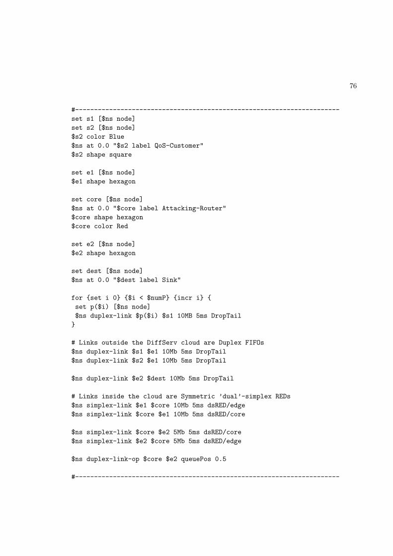
76
#----------------------------------------------------------------------
set s1 [$ns node]
set s2 [$ns node]
$s2 color Blue
$ns at 0.0 "$s2 label QoS-Customer"
$s2 shape square
set e1 [$ns node]
$e1 shape hexagon
set core [$ns node]
$ns at 0.0 "$core label Attacking-Router"
$core shape hexagon
$core color Red
set e2 [$ns node]
$e2 shape hexagon
set dest [$ns node]
$ns at 0.0 "$dest label Sink"
for {set i 0} {$i < $numP} {incr i} {
set p($i) [$ns node]
$ns duplex-link $p($i) $s1 10MB 5ms DropTail
}
# Links outside the DiffServ cloud are Duplex FIFOs
$ns duplex-link $s1 $e1 10Mb 5ms DropTail
$ns duplex-link $s2 $e1 10Mb 5ms DropTail
$ns duplex-link $e2 $dest 10Mb 5ms DropTail
# Links inside the cloud are Symmetric ’dual’-simplex REDs
$ns simplex-link $e1 $core 10Mb 5ms dsRED/edge
$ns simplex-link $core $e1 10Mb 5ms dsRED/core
$ns simplex-link $core $e2 5Mb 5ms dsRED/core
$ns simplex-link $e2 $core 5Mb 5ms dsRED/edge
$ns duplex-link-op $core $e2 queuePos 0.5
#----------------------------------------------------------------------

77
#----------------------------------------------------------------------
#Setup all the queues and policies etc (DiffServ)
set qE1C [[$ns link $e1 $core] queue]
set qE2C [[$ns link $e2 $core] queue]
set qCE1 [[$ns link $core $e1] queue]
set qCE2 [[$ns link $core $e2] queue]
# Set DiffServ RED parameters from Edge1 to Core: $qE1C
meanPktSize $packetSize $qE1C set numQueues_ 1 $qE1C setNumPrec 2
$qE1C addPolicyEntry [$s2 id] [$dest id] TokenBucket 10 $cir1 $cbs1
$qE1C addPolicerEntry TokenBucket 10 11
$qE1C addPolicyEntry -1 [$dest id] TokenBucket 0 $cir0 $cbs0
$qE1C addPolicerEntry TokenBucket 0 0
$qE1C addPHBEntry 10 0 0
$qE1C addPHBEntry 11 0 1
$qE1C addPHBEntry 0 0 1
#Differentiated Forwarding Assurances
$qE1C configQ 0 0 20 40 0.02
$qE1C configQ 0 1 10 20 0.10
# Set DiffServ RED parameters from Edge2 to Core: $qE2C
meanPktSize $packetSize $qE2C set numQueues_ 1 $qE2C setNumPrec 2
$qE2C addPolicyEntry [$dest id] [$s2 id] TokenBucket 10 $cir1 $cbs1
$qE2C addPolicerEntry TokenBucket 10 11
$qE2C addPolicyEntry [$dest id] -1 TokenBucket 0 $cir0 $cbs0
$qE2C addPolicerEntry TokenBucket 0 0
$qE2C addPHBEntry 10 0 0
$qE2C addPHBEntry 11 0 1
$qE2C addPHBEntry 0 0 1
$qE2C configQ 0 0 20 40 0.02
$qE2C configQ 0 1 10 20 0.10
# Set DiffServ RED parameters from Core to Edge1: $qCE1
meanPktSize $packetSize $qCE1 set numQueues_ 1 $qCE1 setNumPrec 2

78
$qCE1 addPHBEntry 10 0 0 $qCE1 addPHBEntry 11 0 1 $qCE1
addPHBEntry 0 0 1 $qCE1 configQ 0 0 20 40 0.02 $qCE1 configQ 0 1
10 20 0.10
# Set DiffServ RED parameters from Core to Edge2: $qCE2
setSchedularMode WRR
#Get the WRR parameters from ratio of TotPkts on qCE2 stats.
$qCE2 addQueueWeights 0 1
$qCE2 addQueueWeights 1 16
$qCE2 meanPktSize $packetSize
$qCE2 set numQueues_ 2
$qCE2 setNumPrec 2
$qCE2 addPHBEntry 10 0 0
$qCE2 addPHBEntry 11 0 1
#BE is put in a separate queue 1 0, to provide
#better B/W sharing b/w S1 and S2 side traffic
$qCE2 addPHBEntry 0 1 0
$qCE2 configQ 0 0 20 40 0.02
$qCE2 configQ 0 1 10 20 0.06
$qCE2 configQ 1 0 10 20 0.10
#----------------------------------------------------------------------
#----------------------------------------------------------------------
set null0 [new Agent/LossMonitor]
$ns attach-agent $dest $null0
for {set i 0} {$i < $numP} {incr i} {
set udp($i) [new Agent/UDP]
$ns attach-agent $p($i) $udp($i)
$udp($i) set class_ [expr $i+1]
$ns color $i Blue
set pareto($i) [new Application/Traffic/Pareto]
$pareto($i) set packetSize_ $packetSize
$pareto($i) set burst_time_ 500ms
$pareto($i) set idle_time_ 500ms
#Set rate apply
$pareto($i) set rate_ 200k

79
$pareto($i) set shape_ 1.4
$pareto($i) attach-agent $udp($i)
$ns connect $udp($i) $null0
}
set udp1 [new Agent/UDP]
$ns attach-agent $s2 $udp1
$udp1 set class_ numP
$ns color numP Red
# CBR or MPEG4 source
#set cbr1 [new Application/Traffic/CBR]
#$cbr1 attach-agent $udp1
#$cbr1 set packet_size_ $packetSize
#$udp1 set packetSize_ $packetSize
#$cbr1 set rate_ $cir1
set tfile [new Tracefile]
$tfile filename Allcap33.trace
set stream [new Application/Traffic/Trace]
$stream attach-tracefile $tfile
$stream attach-agent $udp1
#S2 is sinked in a LossMonitor
set sink0 [new Agent/LossMonitor]
$ns attach-agent $dest $sink0
$ns connect $udp1 $sink0
#----------------------------------------------------------------------
#----------------------------------------------------------------------
#Define a procedure which periodically records the byes/packets
#received by the traffic sink sink0 and writes it to the file f0.
proc record {} {
global sink0 null0 f0
#Get an instance of the simulator
set ns [Simulator instance]
#Call after another 10s
set time 10
set ss0 [$null0 set bytes_]

80
set strm0 [$sink0 set bytes_]
#Get the current time
set now [$ns now]
puts $f0 "50002 $now 25 0 [expr $ss0] [expr $strm0] 0 0"
$null0 set bytes_ 0
$sink0 set bytes_ 0
#Re-schedule the procedure
$ns at [expr $now+$time] "record"
}
#----------------------------------------------------------------------
#----------------------------------------------------------------------
proc finish {} {
global ns f0 nf
$ns flush-trace
close $f0
#Close the trace file
close $nf
#Execute nam on the trace file
#exec nam thesis.nam &
exit 0
}
#----------------------------------------------------------------------
#----------------------------------------------------------------------
#$qE1C printPolicyTable
#$qE1C printPolicerTable
#$qE2C printPolicyTable
#$qE2C printPolicerTable
$ns at 0.0 "record"
for {set i 0} {$i < $numP} {incr i} {
$ns at 0.0 "$pareto($i) start"
}
#$ns at 0.0 "$cbr1 start"
$ns at 0.0 "$stream start"
#Attacks go here (only simplified samples shown for brevity)
#Attacks on Delay and Bandwidth (ldrops) through WRR parameters

81
#$ns at 10000.0 "$qCE2 addQueueWeights 0 1"
#$ns at 10300.0 "$qCE2 addQueueWeights 0 5"
#Attacks through RED parameters causing early drops (edrops)
#$ns at..
#$qCE2 configQ 0 0 20 40 0.10
#$qCE2 configQ 0 1 20 30 0.30
#$qCE2 configQ 1 0 10 20 0.10
for {set i 0} {$i < $numP} {incr i} {
$ns at $testTime "$pareto($i) stop"
}
#$ns at $testTime "$cbr1 stop"
$ns at $testTime "$stream stop"
$ns at $testTime "$qCE2 printStats"
$ns at [expr $testTime + 1.0] "finish"
$ns run
#----------------------------------------------------------------------

82
Appendix B
The MPEG4 NS2 Trace :
Generation and Capture Details
The MPEG-4 NS2 trace used for our simulation tests is due to George Kinal with
Femme Comp, Inc. He captured the original MPEG-4 material, when he was employed by
Airia, Inc. The actual reduction to NS-2 traces was done while he was employed by Femme
Comp, Inc. The following is his description of the source of the MPEG-4 stream, and the
method of capture.
1. The original data source was a Philips Webcine MPEG-4 streaming en-coder, version 1.1. It was encoding a live video feed, specifically the BBC-Worldnews service. The encoder was set to encode this NTSC video with a frame sizeof 320 X 240 pixels. It generated streaming packets compliant with ISMA ver-sion 1.1, sent over a LAN and addressed to a multicast group address. Encodersettings were for the MPEG-4 simple profile (I and P frames only). I believethat the key frames (forced I frames) were set to a 3 second interval. The targetaverage data rate for video was 260k bits/sec2. These streams (RTP/UDP for the video and audio, and SAP/SDP for
broadcast announcement) were captured on a separate computer using a pro-gram called Captureall.exe; each UDP packet addressed to the appropriate mul-ticast address and port was time tagged and saved to a file with an appropriateID header. In this case, the captured file was called ALLCAP33057PM, andrepresented 30 minutes of the program; it is 65 MB.3. A second custom program, ALLCAP to Trace.exe was then written to
parse this file, separating only the video packets, and to write binary trace filecompatible with NS-2 (32 bits for the time stamp in microseconds, and 32 bitsfor the packet size). This packet size includes the encoded video frame as wellas the RTP and UDP headers.

83
Note that the time stamps, although written in microsecond resolution, aregranular to within the limitations of the PC time stamp resolution. There isalso an underlying periodicity of the video frames and packets related to thevideo frame rate of 30 fps (thus, 33 msec).I think these streams and the extracted data are quite representative of
MPEG-4 video streaming, and I also note that Real has just signed up to beMPEG-4 compatible, so their RealVideo streams should become very similar tothese.