Abstract - Brown University · PDF fileAbstract We develop an ... the WENO interpolation of the solution and its derivatives are used to directly ... WENO schemes are high order schemes

An alternative formulation of finite difference WENO schemes with

Lax-Wendroff time discretization for conservation laws

Yan Jiang1, Chi-Wang Shu2 and Mengping Zhang3

Abstract

We develop an alternative formulation of conservative finite difference weighted essen-

tially non-oscillatory (WENO) schemes to solve conservation laws. In this formulation,

the WENO interpolation of the solution and its derivatives are used to directly construct

the numerical flux, instead of the usual practice of reconstructing the flux functions. Even

though this formulation is more expensive than the standard formulation, it does have

several advantages. The first advantage is that arbitrary monotone fluxes can be used in

this framework, while the traditional practice of reconstructing flux functions can be ap-

plied only to smooth flux splitting. The second advantage, which is fully explored in this

paper, is that it is more straightforward to construct a Lax-Wendroff time discretization

procedure, with a Taylor expansion in time and with all time derivatives replaced by spa-

tial derivatives through the partial differential equations, resulting in a narrower effective

stencil compared with previous high order finite difference WENO scheme based on the

reconstruction of flux functions with a Lax-Wendroff time discretization. We will de-

scribe the scheme formulation and present numerical tests for one- and two-dimensional

scalar and system conservation laws demonstrating the designed high order accuracy and

non-oscillatory performance of the schemes constructed in this paper.

Key Words: weighted essentially non-oscillatory scheme, Lax-Wendroff time dis-

cretization, high order accuracy

1School of Mathematical Sciences, University of Science and Technology of China, Hefei, Anhui230026, P.R. China. E-mail: [email protected]

2Division of Applied Mathematics, Brown University, Providence, RI 02912, USA. E-mail:[email protected]. Research supported by AFOSR grant F49550-12-1-0399 and NSF grant DMS-1112700.

3School of Mathematical Sciences, University of Science and Technology of China, Hefei, Anhui230026, P.R. China. E-mail: [email protected]. Research supported by NSFC grants 11071234,91130016 and 91024025.

1

1 Introduction

In this paper, we are interested in designing an alternative formulation of high order

conservative finite difference WENO (weighted essentially non-oscillatory) methods, with

the Lax-Wendroff time discretizations, in solving nonlinear hyperbolic conservation laws

{

ut + ∇ · f(u) = 0u(x, 0) = u0(x).

(1)

On a uniform mesh xi = i∆x, a semi-discrete conservative finite difference scheme

for solving (1) has the following form

d

dtui +

1

∆x

(

fi+ 12− fi− 1

2

)

= 0 (2)

where ui is an approximation to the point value u(xi, t), and the numerical flux

fi+ 1

2= f(ui−r, . . . , ui+s)

is designed so that

1

∆x

(

fi+ 12− fi− 1

2

)

= f(u(x))x|xi+ O(∆xk) (3)

for a k-th order scheme. Most of the high order finite difference schemes, for example

the high order finite difference WENO schemes in [4, 1, 12], use the following simple

Lemma in [14]:

Lemma 1.1 (Shu and Osher [14]): If a function h(x) satisfies the following relationship

f(u(x)) =1

∆x

∫ x+∆x2

x−∆x2

h(ξ)dξ (4)

then

1

∆x

(

h(x +∆x

2) − h(x −

∆x

2)

)

= f(u(x))x. (5)

The proof of this lemma is a simple application of the fundamental theorem of cal-

culus.

2

With this simple lemma, it is clear that we should take the numerical flux as

fi+ 12

= h(xi+ 12) + O(∆xk) (6)

with a smooth coefficient in the O(∆xk) term, to obtain the high order accuracy (3).

Since the definition of the function h(x) in (4) implies

hi =1

∆x

∫ xi+1

2

xi−1

2

h(ξ)dξ = f(ui)

which is known once we have the point values ui, we are facing the standard recon-

struction problem of knowing the cell averages {hi} of the function h(x), and seeking to

reconstruct its point values at the cell boundaries h(xi+ 12) to high order accuracy, to be

used as the numerical flux fi+ 12

in (6). This reconstruction problem is the backbone of

the standard finite volume schemes, for example the essentially non-oscillatory (ENO)

finite volume schemes [3] and WENO finite volume schemes [7]. Therefore, using the

simple Lemma 1.1, we can simply apply the standard reconstruction subroutine in a

high order finite volume scheme to obtain the numerical flux {fi+ 12} for a high order

conservative finite difference scheme from the flux point values {f(ui)}.

Because of the clean conception and easy implementation, this formulation of numer-

ical fluxes in high order conservative finite difference schemes has been used widely, for

example in high order finite difference ENO schemes [14] and WENO schemes [4, 1, 12].

However, there are several disadvantages of this formulation:

1. In order to achieve upwinding and nonlinear stability, an approximate Riemann

solver or a two-point monotone flux is used in finite volume schemes. With this

finite difference flux formulation, upwinding can be implemented easily only for

the following smooth flux splitting

f(u) = f+(u) + f−(u)

where ddu

f+(u) ≥ 0 (or in system case, this Jacobian matrix has only real and

positive eigenvalues) and ddu

f−(u) ≤ 0 (or in system case, this Jacobian matrix has

3

only real and negative eigenvalues). In order to guarantee high order accuracy, the

two functions f+(u) and f−(u) should be as smooth functions of u as f(u). The

most common flux splitting used in finite difference schemes is therefore the Lax-

Friedrichs flux splitting, which is the most diffusive among two-point monotone

fluxes.

2. The Lax-Wendroff time discretization procedure [8] is difficult to design and results

in a rather wide effective stencil. We will elaborate in more details on this point

later in the paper.

3. Since the reconstruction is performed directly on the flux values {f(ui)} (or {f+(ui)}

and {f−(ui)} with flux splitting), not on the point values of the solution {ui}, it

is more difficult to maintain free stream solutions exactly in curvilinear meshes

for multi-dimensional flow computation. This is because the fluxes in curvilinear

coordinates involve metric derivatives, resulting in non-exact cancellations when

nonlinear reconstructions are performed for different fluxes.

We would like to explore an alternative formulation for constructing numerical fluxes

in high order conservative finite difference schemes, originally designed in [13], which

involves interpolations directly on the point values of the solution {ui} rather than on

the flux values. This alternative formulation, even though less clean and more computa-

tionally expensive, does overcome all three disadvantages listed above. We will explore

the overcoming of the first two disadvantages, especially the second one, in detail in this

paper.

We now give a brief survey of WENO schemes and Lax-Wendroff time discretiza-

tion. WENO schemes are high order schemes for approximating hyperbolic conservation

laws and other convection dominated partial differential equations. They can produce

sharp, non-oscillatory discontinuity transitions and high order accurate resolutions for

the smooth part of the solution. The first WENO scheme was introduced in 1994 by

4

Liu, Osher and Chan in their pioneering paper [7], in which a third order accurate fi-

nite volume WENO scheme in one space dimension was constructed. In [4], a general

framework is provided to design arbitrary high order accurate finite difference WENO

schemes, which are more efficient for multi-dimension calculations. Very high order finite

difference WENO schemes are documented in [1].

The Lax-Wendroff time discretization procedure, which is also called the Taylor type

time discretization, is based on the idea of the classical Lax-Wendroff scheme [5], relying

on writing the solution at the next time step by Taylor expansion in time, and repeatedly

using the partial differential equation (PDE) to rewrite the time derivatives in this Taylor

expansion as spatial derivatives. These spatial derivatives can then be discretized by

standard approximation procedures, for example the WENO approximation. We denote

uni as the approximation of the point values u(xi, t

n), and u(r) as the r-th order time

derivative of u, namely u(r) = ∂ru∂tr

. We also use u′, u′′ and u′′′ to denote the first three

time derivatives of u. By Taylor expansion, we obtain

u(x, t + ∆t) = u(x, t) + ∆tu′ +∆t2

2!u′′ +

∆t3

3!u′′′ +

∆t4

4!u(4) +

∆t5

5!u(5) + · · · . (7)

If we approximate the first k derivatives, we can get k-th order accuracy in time. The

main idea of the Lax-Wendroff time discretization procedure is to rewrite the time deriva-

tives u(r) as spatial derivatives utilizing the PDE, then discretize these spatial derivatives

to sufficient accuracy. This is rather straightforward for a finite volume scheme. However,

for a finite difference scheme using the formulation (6) and Lemma 1.1 to compute its

numerical fluxes, it is more difficult to implement the Lax-Wendroff procedure because

we do not have approximations to the spatial derivatives of the solution u at our disposal,

only approximations to the spatial derivatives of the flux function f(u). In [8], Qiu and

Shu designed a finite difference WENO scheme with Lax-Wendroff time discretization

using the formulation (6) and Lemma 1.1. To avoid the difficulty mentioned above, they

use the approximations to the lower order time derivatives to approximate the higher

order ones. As a consequence, the method in [8] involves a rather wide effective stencil.

5

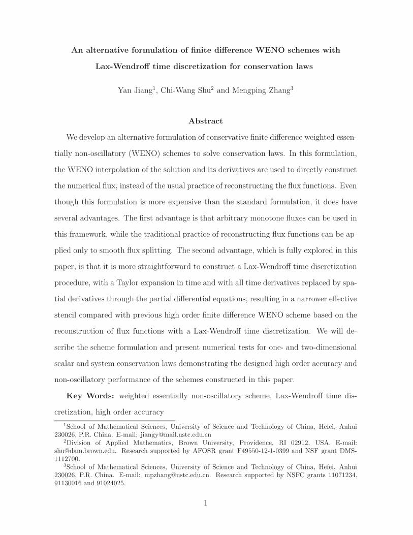
We will provide more details to illustrate this phenomenon. In the procedure to build a

fifth order in space and fourth order in time scheme in [8] for solving the one-dimensional

scalar equation ut + f(u)x = 0, the following steps are involved:

Step 1. Using the PDE, we obtain u′ = −f(u)x, and the first order time derivative

can be obtained by the conservative finite difference WENO approximation (3). To

obtain a fifth order WENO approximation for u′|nj , we would need the point values

S = {unj−3, · · · , un

j+3}.

Step 2. When constructing the second order time derivative u′′ = −(f ′(u)u′)x, we denote

gj = f ′(uj)u′j, where u′

j are the point values of the first order time derivative computed

in the previous Step 1. Then we can use a fourth order central difference formula to

approximate u′′ = −gx at the point (xj , tn):

u′′j = −

1

12∆x(gj−2 − 8gj−1 + 8gj+1 − gj+2).

It was observed in [8] that the more costly WENO approximation is not necessary for

second and higher order time derivatives, as the standard central difference approxima-

tions perform well. Considering gj = f ′(uj)u′j and using Step 1 to obtain u′

j, we have

the effective stencil for obtaining the point value u′′|nj to be S = {unj−5, · · · , un

j+5}.

Step 3. When constructing the third order time derivative u′′′ = −(f ′(u)u′′+f ′′(u)(u′)2)x,

we let gj = (f ′(uj)u′′j + f ′′(uj)(u

′)2j ), where the point values u′

j and u′′j are obtained in

the previous Step 1 and Step 2, respectively. Then we repeat Step 2 to approximate the

third order time derivative using a fourth order central difference approximation (third

order accuracy is enough here, but central approximations provide only even orders of

accuracy). Considering u′j and u′′

j are obtained in Step 1 and Step 2, we obtain the

effective stencil for approximating u′′′ at the point (xj , tn) to be S = {un

j−7, · · · , unj+7}.

Step 4. The construction of the fourth order time derivative u(4) = −(f ′(u)u′′′ +

3f ′′(u)u′u′′+f ′′′(u)(u′)3)x is obtained in a similar fashion. Let gj = f ′(uj)u′′′j +3f ′′(uj)u

′ju

′′j+

6

f ′′′(uj)(u′)3

j , where the point values u′j , u′′

j and u′′′j are obtained in the previous Steps

1, 2 and 3 respectively. Then we use a second order central difference to approximate

u(4)j = − 1

2∆x(gj+1 − gj−1). Thus, to get the value u(4) at the point (xj , t

n), we actually

need point values in the effective stencil S = {unj−8, · · · , un

j+8}.

In summary, to obtain a fifth order in space and fourth order in time Lax-Wendroff

type WENO scheme in [8], the effective stencil is S = {Ij−8, · · · , Ij+8} for the point xj ,

containing 17 grid points. This is a pretty wide stencil. Of course, it is still narrower

than Runge-Kutta time discretization. When a four-stage, fourth order Runge-Kutta

time discretization is used on a fifth order finite difference WENO scheme, the width of

the effective stencil is 25 grid points.

One major motivation to discuss the alternative formulation of high order conser-

vative finite difference schemes in this paper is to make the effective stencil narrower

when applying the Lax-Wendroff time discretization. We will review WENO interpola-

tion in Section 2, which is the main approximation tool for the alternative formulation

of high order conservative finite difference schemes. Details on the construction and

implementation of the alternative formulation will be described in Section 3, for one-

and two-dimensional scalar and system equations. In Section 4, extensive numerical

examples are provided to demonstrate the accuracy and effectiveness of the methods.

Concluding remarks are given in Section 5.

2 WENO interpolation

A major building block of the alternative formulation of high order conservative finite

difference scheme discussed in this paper is the following WENO interpolation procedure.

Given the point values ui = u(xi) of a piecewise smooth function u(x), we would like

to find an approximation of u(x) at the half nodes xi+ 12. This WENO interpolation

procedure has been developed in, e.g. [10, 2, 12] and will be described briefly below.

The first component of the general WENO produce is a set of lower order approxi-

7

mations to the target value, based on different stencils, which are referred to as the small

stencils. We would find a unique polynomial of degree at most k − 1, denoted by pr(x),

which interpolates the function u(x), namely pr(xj) = uj, at the mesh points xj in the

small stencil Sr = {xi−r, xi−r+1, . . . , xi+s} for r = 0, 1, . . . , k − 1, with r + s + 1 = k.

Then, we would use u(r)

i+ 12

= pr(xi+ 12) as an approximation to the value u(xi+ 1

2), and we

have

u(r)

i+ 12

− u(xi+ 12) = O(∆xk) (8)

if the function u(x) is smooth in the stencil Sr. For example, when k = 3, we have

S0 = {xi, xi+1, xi+2}, S1 = {xi−1, xi, xi+1}, S2 = {xi−2, xi−1, xi}, and

u(0)

i+ 12

=3

8ui +

3

4ui+1 −

1

8ui+2,

u(1)

i+ 12

= −1

8ui−1 +

3

4ui +

3

8ui+1,

u(2)

i+ 1

2

=3

8ui−2 −

5

4ui−1 +

15

8ui.

The second component of the general WENO procedure is to combine the set of lower

order approximations to form a higher order approximation to the same target value,

based on the big stencil S = {xi−k+1, . . . , xi+k−1}, which is the union of all the small

stencils in the first component. We would find a unique polynomial of degree at most

2k − 2, denoted by p(x), interpolating the function u(x) at the points in the big stencil.

We use ui+ 12

= p(xi+ 12) as the approximation to the value u(xi+ 1

2), and we have

ui+ 1

2− u(xi+ 1

2) = O(∆x2k−1) (9)

provided that the function u(x) is smooth in the big stencil S. When k = 3, we have

ui+ 12

=3

128ui−2 −

5

32ui−1 +

45

64ui +

15

32ui+1 −

5

128ui+2.

There are constants dr such that

ui+ 12

=k−1∑

r=0

dru(r)

i+ 12

(10)

8

where the constants satisfy∑k−1

r=0 dr = 1. These constants are usually referred as the

linear weights in the WENO procedure. For the case k = 3, the linear weights are given

as

d0 =5

16, d1 =

5

8, d2 =

1

16.

The third component of the general WENO procedure is to change the linear weights

into nonlinear weights, to ensure both accuracy in smooth cases and non-oscillatory

performance when at least one of the small stencils contain a discontinuity of the function

u(x). We can achieve this through changing the linear weights dr into the nonlinear

weights ωr, defined by

ωr =αr

∑k−1s=0 αs

, r = 0, . . . , k − 1 (11)

with

αr =dr

(ǫ + βr)2. (12)

Here, we take ǫ = 10−6, avoiding the denominator to be zero, and βr are the so-called

smoothness indicators of the stencil Sr, which measures the smoothness of u(x) in this

stencil. Following the original WENO recipe [4], we define

βr =

k−1∑

l=1

∫ xi+ 1

2

xi− 1

2

∆x2l−1

(

∂lpr(x)

∂lx

)2

dx. (13)

When k = 3, the formula gives

β0 =13

12(ui − 2ui+1 + ui+2)

2 +1

4(3ui − 4ui+1 + ui+2)

2,

β1 =13

12(ui−1 − 2ui + ui+1)

2 +1

4(ui−1 − ui+1)

2,

β2 =13

12(ui−2 − 2ui−1 + ui)

2 +1

4(ui−2 − 4ui−1 + 3ui)

2.

Thus, we get the WENO interpolation of u(x) at the point xi+ 12

as

ui+ 12

=k−1∑

r=0

ωru(r)

i+ 12

. (14)

9

We denote it by u−

i+ 12

since the big stencil S used to obtain this approximation is biased

to the left (there is one more grid point to the left of xi+ 12

than to the right). If u(x) is

smooth in this big stencil S, we have

u−

i+ 12

− u(xi+ 1

2) = O(∆x2k−1).

If one of the small stencils contains a discontinuity, the corresponding smoothness indica-

tor will be much larger than that of other small stencils, hence the nonlinear weight corre-

sponding to this small stencil will be very small, thus achieving essentially non-oscillatory

performance. If we choose the big stencil as S = {xi−k+2, . . . , xi+k} which is biased to

the right, and the small stencils as Sr = {xi−r+1, . . . , xi−r+k}, for r = 0, . . . , k − 1, we

can obtain in a similar fashion a WENO interpolation of u(x) at the point xi+ 12, denoted

by u+i+ 1

2

, which has the same high order accuracy in smooth regions and essentially non-

oscillatory performance near discontinuities as u−

i+ 12

. In fact, the process to obtain u+i+ 1

2

is mirror-symmetric to that for u−

i+ 12

, with respect to the target point xi+ 12.

3 Construction of the scheme

3.1 Construction of the numerical flux in one-dimension

Assuming that f(u) is a smooth function of u, we would like to find a consistent numerical

flux function

fi+ 12

= f(ui−r, . . . , ui+s), (15)

such that the flux difference approximates the derivative f(u(x))x to k-th order accuracy

1

∆x(fi+ 1

2− fi− 1

2) = f(u(x))x|xi

+ O(∆xk). (16)

The numerical flux should satisfy the following conditions:

• f is a Lipschitz continuous function in all the arguments;

• f is consistent with the physical flux f , that is, f(u, · · · , u) = f(u).

10

It has been shown in [13] that there exist constants a2, a4, . . . such that

fi+ 12

= fi+ 12

+

[(r−1)/2]∑

k=1

a2k∆x2k

(

∂2k

∂x2kf

)

i+ 1

2

+ O(∆xr+1) (17)

which guarantees k = r-th order accuracy in (16). The coefficients a2r in (17) can

be obtained through Taylor expansion and the accuracy constraint (16). To get an

approximation with fifth order accuracy (k = 5 in (16)), we can use the first three terms

given as

fi+ 12

= fi+ 12−

1

24∆x2fxx|i+ 1

2+

7

5760∆x4fxxxx|i+ 1

2. (18)

The first term of the numerical flux in (18) is approximated by

fi+ 12

= h(u−

i+ 12

, u+i+ 1

2

) (19)

with the values u±

i+ 12

obtained by the WENO interpolation discussed in the previous

section. The two-argument function h is a monotone flux. It satisfies:

• h(a, b) is a Lipschitz continuous function in both argument;

• h(a, b) is a nondecreasing function in a and a nonincreasing function in b. Symbol-

ically h(↑, ↓);

• h(a, b) is consistent with the physical flux f , that is, h(a, a) = f(a).

Examples of the monotone fluxes include:

1. The Godunov flux:

h(a, b) =

{

mina≤x≤b f(u), if a ≤ bmaxb≤x≤a f(u), if a > b

(20)

2. The Engquist-Osher flux:

h(a, b) =

∫ a

0

max(f ′(u), 0)du +

∫ b

0

min(f ′(u), 0)du + f(0) (21)

11

3. The Lax-Friedrichs flux:

h(a, b) =1

2[f(a) + f(b) − α(b − a)] (22)

where α = maxu |f′(u)| is a constant. The maximum is taken over the relevant

range of u.

More discussions on monotone fluxes can be found in, e.g. [6].

The remaining terms of the numerical flux in (18) have at least ∆x2 in their co-

efficients, hence they only need lower order approximations and they are expected to

contribute much less to spurious oscillations. Therefore, following the practice in [8],

we approximate these remaining terms by simple central approximation or one-point

upwind-biased approximation with suitable orders of accuracy, without using the more

expensive WENO procedure.

3.2 One-dimensional scalar case

Consider the one-dimension scalar conservation law

{

ut + f(u)x = 0,u(x, 0) = u0(x).

(23)

We describe the Lax-Wendroff time discretization to get k-th order accuracy in time. In

this paper, we will implement the procedure up to fourth order in time.

1. The approximation of the first time derivative u′ = −f(u)x follows the standard

WENO procedure. We construct the numerical flux with (2r−1)-th order accuracy

as described in the previous section. In particular, the points {xi−r+1, . . . , xi+r}

are required to obtain the WENO interpolation u±

i+ 1

2

. For the spatial derivatives

∂kf∂xk at xi+ 1

2, we use (2r − 1 − k)-th order simple finite difference approximations

based on the same points {xi−r+1, . . . , xi+r}. In our numerical experiments, we aim

for fifth order spatial accuracy and take r = 3. The numerical flux corresponding

12

to u′ is then given as

f(1)

i+ 12

= h(u−

i+ 12

, u+i+ 1

2

) −1

24∆x2(f ′′(u)(ux)

2 + f ′(u)uxx)|xi+1

2

+7

5760∆x4(f ′′′′(u)(ux)

4

+ 6f ′′′(u)(ux)2uxx + 4f ′′(u)uxuxxx + 3f ′′(u)(uxx)

2 + f ′(u)uxxxx)|xi+ 1

2

such that

f(1)

i+ 12

− f(1)

i− 12

∆x= −u′|xi

+ O(∆x4)

where u±

i+ 1

2

in the h(u−

i+ 1

2

, u+i+ 1

2

) term are obtained through the fifth order WENO

interpolation, and the values of u, ux, uxx, uxxx and uxxxx at xi+ 12

in the remaining

terms are obtained from the same polynomial interpolation based on the points

{xi−2, . . . , xi+3}.

2. The next step is to obtain the approximation of the second time derivative u′′ =

−(f ′(u)u′)x = ((f ′(u))2ux)x. We let g = −(f ′(u))2ux, and repeat the process in

Step 1. The two major differences from Step 1 are: (i) the approximation can

be one order lower in accuracy since there is an extra ∆t in the coefficient; and

(ii) there is no need to involve WENO in the approximation, also because of the

extra ∆t in the coefficient. Therefore, we would still only need the interpolation

polynomial based on the points {xi−2, . . . , xi+3} for all the values of u, ux, uxx,

uxxx and uxxxx at xi+ 1

2in the following expression

f(2)

i+ 12

= g|xi+1

2

−∆x2

24gxx|x

i+12

= −(f ′(u))2ux|xi+1

2

+∆x2

24(2(f ′′(u))2(ux)

3 + 2f ′′′(u)f ′(u)(ux)3

+ 6f ′′(u)f ′(u)uxuxx + (f ′(u))2uxxx)|xi+1

2

such that

f(2)

i+ 12

− f(2)

i− 12

∆x= −u′′|xi

+ O(∆x4).

13

3. The approximation of the third time derivative u′′′ = −(3f ′′(u)(f ′(u))2u2x

+ (f ′(u))3uxx)x is obtained in a similar fashion. Let g = (3f ′′(u)(f ′(u))2

u2x + (f ′(u))3uxx), we can obtain the numerical flux as

f(3)

i+ 12

=g|xi+1

2

−∆x2

24gxx|x

i+ 12

=(3f ′′(u)(f ′(u))2(ux)2 + (f ′(u))3uxx)|x

i+12

−∆x2

24(3f ′′′′(u)(f ′(u))2(ux)

4

+ 18f ′′′(u)f ′′(u)f ′(u)(ux)4 + 18f ′′′(u)(f ′(u))2(ux)

2uxx + 6(f ′′(u))3(ux)4

+ 36(f ′′(u))2f ′(u)(ux)2uxx + 12f ′′(u)(f ′(u))2uxuxxx + 9f ′′(u)(f ′(u))2(uxx)

2

+ (f ′(u))3uxxxx)|xi+1

2

where the values of u, ux, uxx, uxxx and uxxxx at xi+ 12

can all be obtained from the

same interpolation polynomial based on the points {xi−2, . . . , xi+3}. We will then

have

f(3)

i+ 12

− f(3)

i− 12

∆x= −u′′′|xi

+ O(∆x3)

4. The final step is the approximation of the fourth time derivative u(4) = (4f ′′′(u)(f ′(u))3

(ux)3 + 12(f ′′(u))2(f ′(u))2(ux)

3 + 12f ′′(u)(f ′(u))3uxuxxx + (f ′(u))4uxxx)x. Let g =

−(4f ′′′(u)(f ′(u))3(ux)3+12(f ′′(u))2(f ′(u))2(ux)

3+12f ′′(u)(f ′(u))3uxuxxx+(f ′(u))4uxxx),

we can obtain the numerical flux as

f(4)

i+ 1

2

=g|xi+1

2

= − (4f ′′′(u)(f ′(u))3(ux)3 + 12(f ′′(u))2(f ′(u))2(ux)

3 + 12f ′′(u)(f ′(u))3uxuxxx

+ (f ′(u))4uxxx)|xi+1

2

where the values of u, ux, uxx, uxxx and uxxxx at xi+ 12

can all be obtained from the

same interpolation polynomial based on the points {xi−2, . . . , xi+3}. We will then

have

f(4)

i+ 12

− f(4)

i− 12

∆x= −u(4)|xi

+ O(∆x2).

14

5. We can form the numerical flux as the sum of all the fluxes above

fi+ 12

= f(1)

i+ 12

+∆t

2f

(2)

i+ 12

+∆t2

6f

(3)

i+ 12

+∆t3

24f

(4)

i+ 12

and obtain the final scheme

un+1i = un

i −∆t

∆x

(

fi+ 12− fi− 1

2

)

which is fifth order accurate in space and fourth order accurate in time.

Of course, we can also increase the time accuracy to fifth order, however heavier

algebra will be involved. In practice, the time accuracy can usually be lower than spatial

accuracy to achieve the desired resolution on modest meshes. This is also verified in our

numerical results in Section 4.

Clearly, the fifth order in space, fourth order in time Lax-Wendroff finite difference

scheme constructed above has an effective stencil of only 7 points, the same as the semi-

discrete scheme. This compares quite favorably with the Lax-Wendroff type scheme

in [8] which has an effective stencil of 17 points, or a fourth order Runge-Kutta finite

difference WENO scheme which has an effective stencil of 25 points.

3.3 One-dimensional systems

For a one-dimensional system of conservation laws (23),

u(x, t) = (u1(x, t), · · · , um(x, t))T (24)

is a vector and

f(u) = (f 1(u1, · · · , um), · · · , fm(u1, · · · , um))T (25)

is a vector function of u. Suppose the system is hyperbolic, i.e. the Jacobian f ′(u) has

m real eigenvalues

λ1(u) ≤ . . . ≤ λm(u) (26)

15

and a complete set of independent eigenvectors

r1(u), . . . , rm(u). (27)

We denote the matrix whose columns are eigenvectors by

R(u) = (r1(u), . . . , rm(u)). (28)

Then

R−1(u)f ′(u)R(u) = Λ(u) (29)

where Λ(u) is the diagonal matrix with λ1(u), . . . , λm(u) on the diagonal.

Similar to the scale case, we replace the time derivatives by spatial derivatives using

the PDE. We still use the numerical flux for each component

gi+ 12

= gi+ 12

+

[(r−1)/2]∑

k=1

a2k∆x2k ∂2kg

∂x2k|i+ 1

2+ O(∆xr+1) (30)

when approaching gx.

When constructing the first part of numerical flux for ut, i.e. h(u−

i+ 12

, u+i+ 1

2

) in f(1)

i+ 12

,

we could use the WENO interpolation procedure on each component of u as in the

scalar case. However, for strong shocks this procedure may lead to oscillatory results.

Interpolation in the local characteristic fields, even though more costly, may effectively

eliminate such spurious oscillations. The procedure of interpolation in the local charac-

teristic fields can be summarized as follows. At each point xi+ 12

where the computation

of the numerical flux is needed, we perform the following steps.

1. Compute an average state ui+ 12, using either the simple arithmetic mean

ui+ 1

2=

1

2(ui + ui+1),

or a Roe average [9] satisfying

f(ui+1) − f(ui) = f ′(ui+ 12)(ui+1 − ui)

if it is available.

16

2. Compute the right eigenvectors and the left eigenvectors of the Jacobian f ′(ui+ 12),

and denote them by

R = R(ui+ 1

2), R−1 = R−1(ui+ 1

2).

3. Transform all the point values which are in the potential stencil of the WENO

interpolation for the obtaining u±

i+ 12

, to the local characteristic fields. For our fifth

order scheme, we need to compute

vj = R−1uj, j = i − 2, ..., i + 3. (31)

4. Perform the scalar WENO interpolation procedure for each component of the char-

acteristic variable v, to obtain the corresponding component of the interpolation

v±

i+ 12

.

5. Transform back into physical space

u±

i+ 12

= Rv±

i+ 12

..

For the two-argument flux h(u−, u+), instead of the monotone fluxes for the scalar

case, we can choose from a variety of numerical fluxes based on exact or approximate

Riemann solvers [15]. For example, we can use the Godunov flux, the Lax-Friedrichs

flux, the HLLC flux, etc. This is one of the advantages of the alternative formulation

discussed in this paper.

For all remaining terms in the Lax-Wendroff process, we can use simple interpola-

tion polynomials based on the same stencil {xi−2, . . . , xi+3} component-wise to obtain

approximations to the values of u, ux, uxx, uxxx and uxxxx at xi+ 1

2. No characteristic

decomposition or WENO is needed. We remark that in the algebraic manipulations of

the Lax-Wendroff process, the derivatives f ′(u), f ′′(u), f ′′′(u) etc. will become matrices

and higher order tensors, increasing the algebraic complexity of the final formulas.

17

3.4 Two-dimensional cases

Consider the two-dimensional conservation laws:

{

ut + f(u)x + g(u)y = 0,u(x, y, 0) = u0(x, y).

(32)

The same Taylor expansion still gives

u(x, y, t + ∆t) = u(x, y, t) + ∆tu′ +∆t2

2u′′ +

∆t3

6u′′′ +

∆t4

24u(4) + · · · (33)

and we would still like to use the PDE to replace time derivatives by spatial derivatives.

The first time derivative u′ = −f(u)x − g(u)y can be approximated in a dimension-by-

dimension fashion as in standard finite difference schemes [13]. For example, for the fifth

order case, we have

f(1)

i+ 12,j

=h1(u−

i+ 12,j, u+

i+ 12,j) −

∆x2

24(f ′′(u)(ux)

2 + f ′(u)uxx)|(xi+ 1

2,yj) +

7∆x4

5760(f ′′′′(u)(ux)

4

+ 6f ′′′(u)(ux)2uxx + 3f ′′(u)(uxx)

2 + 4f ′′(u)uxuxxx + f ′(u)uxxxx)|(xi+1

2,yj)

g(1)

i,j+ 12

=h2(u−

i,j+ 12

, u+i,j+ 1

2

) −∆y2

24(g′′(u)(uy)

2 + g′(u)uyy)|(xi,yj+12) +

7∆y4

5760(g′′′′(u)(uy)

4

+ 6g′′′(u)(uy)2uyy + 3g′′(u)(uyy)

2 + 4g′′(u)uyuyyy + g′(u)uyyyy)|(xi,yj+ 12)

such that

f(1)

i+ 12,j− f

(1)

i− 12,j

∆x= f(u)x|(xi,yj) + O(∆x5),

g(1)

i,j+ 12

− g(1)

i,j− 12

∆y= g(u)y|(xi,yj) + O(∆y5),

and the values of u±

i+ 12,j, u±

i,j+ 12

in the monotone fluxes h1(·, ·) (approximating f(u))

and h2(·, ·) (approximating g(u)) are obtained by one-dimensional WENO interpolation

in the same procedure as in the one-dimensional case. The values of u and all its

spatial derivatives in all the remaining terms are approximated by simple one-dimensional

polynomial interpolations on the same stencil as the WENO approximation, namely on

S = {xi−2, . . . , xi+3} for fixed yj or on {yj−2, . . . , yj+3} for fixed xi. This part is also the

same as in the one-dimensional case.

18

For the second time derivative, u′′ = (f ′(u)2ux + f ′(u)g′(u)uy)x + (g′(u)f ′(u)ux +

g′(u)2uy)y, we can also approximate them in a dimension-by-dimension fashion. For the

fifth order scheme, the numerical fluxes have the following form:

f(2)

i+ 1

2,j

= − (f ′(u)2ux + f ′(u)g′(u)uy)|(xi+ 1

2,yj) +

∆x2

24(2f ′(u)f ′′′(u)(ux)

3 + 2(f ′′(u))2(ux)3

+ 6f ′(u)f ′′(u)uxuxx + (f ′(u))2uxxx + f ′′′(u)g′(u)(ux)2uy + 2f ′′(u)g′′(u)(ux)

2uy

+ f ′(u)g′′′(u)(ux)2uy + f ′′(u)g′(u)uxxuy + f ′(u)g′′(u)uxxuy

+ 2f ′′(u)g′(u)uxuxy + 2f ′(u)g′′(u)uxuxy + f ′(u)g′(u)uxxy)|(xi+1

2,yj)

g(2)

i,j+ 12

= − (g′(u)f ′(u)ux + (g′(u))2uy)|(xi,yj+12) +

∆y2

24(2g′(u)g′′′(u)(uy)

3 + 2(g′′(u))2(uy)3

+ 6g′(u)g′′(u)uyuyy + (g′(u))2uyyy + g′′′(u)f ′(u)ux(uy)2 + 2g′′(u)f ′′(u)ux(uy)

2

+ g′(u)f ′′′(u)ux(uy)2 + g′′(u)f ′(u)uxuyy + g′(u)f ′′(u)uxuyy

+ 2g′′(u)f ′(u)uyuxy + 2g′(u)f ′′(u)uyuxy + g′(u)f ′(u)uxyy)|(xi,yj+12)

which satisfies

f(2)

i+ 12,j− f

(2)

i− 12,j

∆x= −(f ′(u)2ux + f ′(u)g′(u)uy)x|(xi,yj) + O(∆x4) + O(∆y4)

g(2)

i,j+ 12

− g(2)

i,j− 12

∆y= −(g′(u)f ′(u)ux + g′(u)2uy)y|(xi,yj) + O(∆x4) + O(∆y4).

All the spatial derivatives can be obtained by using simple one- or two-dimensional

polynomial interpolations on the same stencil as the WENO approximation. Two-

dimensional interpolation on the stencil S = {xi−2, . . . , xi+3}×{yj−2, . . . , yj+3} is needed

to obtain approximations of the mixed derivatives. This part is different from the one-

dimensional case. The higher order time derivatives can be approximated in a similar

way.

Once the fluxes for all the time derivatives have been obtained, we can form the final

numerical flux as the sum of all these fluxes

fi+ 12,j = f

(1)

i+ 12,j

+∆t

2f

(2)

i+ 12,j

+∆t2

6f

(3)

i+ 12,j

+∆t3

24f

(4)

i+ 12,j

gi,j+ 12

= g(1)

i,j+ 12

+∆t

2g

(2)

i,j+ 12

+∆t2

6g

(3)

i,j+ 12

+∆t3

24g

(4)

i,j+ 12

19

and obtain the final scheme

un+1i,j = un

i,j −∆t

∆x

(

fi+ 12,j − fi− 1

2,j

)

−∆t

∆y

(

gi,j+ 12− gi,j− 1

2

)

which is fifth order accurate in space and fourth order accurate in time.

For the system case, WENO interpolation with local characteristic decomposition is

still needed for the computation of u±

i+ 1

2,j

and u±

i,j+ 1

2

in the two-point fluxes h1(·, ·) and

h2(·, ·). This part is the same as in the one-dimensional case and uses the information

of the Jacobians f ′(u) and g′(u) in the x and y directions respectively. For all the other

terms, neither local characteristic decomposition nor WENO interpolation is needed.

We can use the interpolation polynomials as described above for the scalar case in each

component of the solution u.

4 Numerical results

In this section, we present the results of our numerical experiments for the schemes

described in the previous section, with fourth order in temporal and fifth order in spatial

accuracy. In some examples we also compare with the Lax-Wendroff type finite difference

WENO scheme in [8], also with fourth order in temporal and fifth order in spatial

accuracy.

Example 1. We first test the accuracy of the scheme on the linear scalar problem

ut + ux = 0 (34)

with the initial condition u(x, 0) = sin(πx) and 2-periodic boundary condition. The exact

solution is u(x, t) = sin(π(x − t)). In Table 1, we show the errors at time t = 2. We

can observe fifth order accuracy until quite refined meshes, despite of the formal fourth

order temporal accuracy, supporting our claim before that spatial errors are usually

dominating for modest meshes.

20

Table 1: Accuracy on ut + ux = 0 with u(x, 0) = sin(πx) at t = 2.

Nx L1 errors order L∞ error order

10 2.38E-02 – 3.67E-02 –20 1.12E-03 4.41 1.99E-03 4.2040 3.45E-05 5.02 6.64E-05 4.9180 1.07E-06 5.00 2.16E-06 4.94160 3.35E-08 5.00 6.51E-08 5.05320 1.05E-09 5.00 1.95E-09 5.06640 3.25E-11 5.01 5.71E-11 5.10

Example 2. We test our scheme on the nonlinear Burgers equation

ut +

(

u2

2

)

x

= 0 (35)

with the initial condition u(x, 0) = 0.5 + sin(πx) and a 2-periodic boundary condition.

All the three monotone fluxes mentioned in Section 3.1, namely the Godunov flux, the

Engquist-Osher flux and the Lax-Friedrichs flux, are tested.

When t = 0.5/π the solution is still smooth. The errors for all three monotone fluxes

are shown in Tables 2 and 3 respectively. For comparison, we also show the errors by

the Lax-Wendroff type finite difference WENO scheme in [8] with the same fourth order

in temporal and fifth order in spatial accuracy in Table 2. We observe that all schemes

achieve fifth order accuracy, despite of the formal fourth order temporal accuracy, once

again supporting our claim before that spatial errors are usually dominating for modest

meshes. For this test case, there is very little difference in the errors corresponding to

the three different monotone fluxes. We do observe that the errors of the WENO scheme

in [8] are significantly bigger than those for the schemes designed in this paper in Tables

2 and 3 when compared on the same mesh, indicating that the narrower effective stencil

and flexibility in choosing numerical fluxes are helping to improve the magnitude of the

errors.

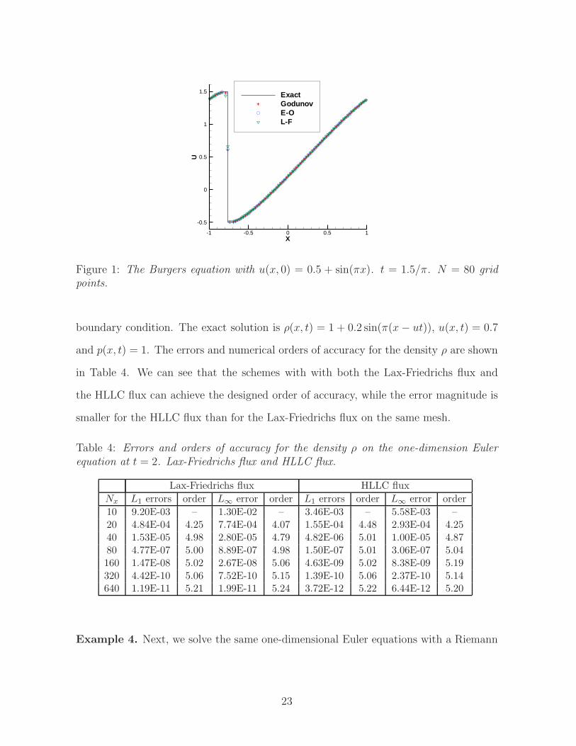
We plot the solution with 80 grid points at time t = 1.5/π in Figure 1, when a

shock has already appeared in the solution. We can see that for all the three monotone

fluxes, the schemes simulate the solution with good resolution and without noticeable

21

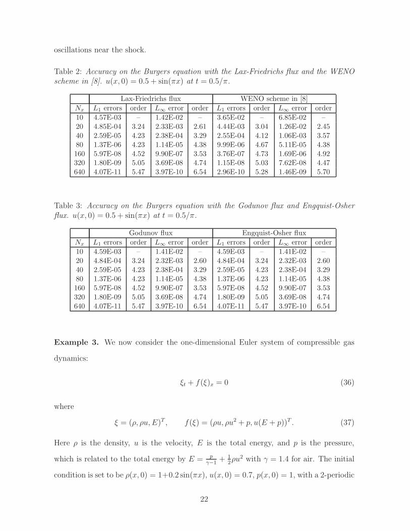
oscillations near the shock.

Table 2: Accuracy on the Burgers equation with the Lax-Friedrichs flux and the WENOscheme in [8]. u(x, 0) = 0.5 + sin(πx) at t = 0.5/π.

Lax-Friedrichs flux WENO scheme in [8]

Nx L1 errors order L∞ error order L1 errors order L∞ error order

10 4.57E-03 – 1.42E-02 – 3.65E-02 – 6.85E-02 –20 4.85E-04 3.24 2.33E-03 2.61 4.44E-03 3.04 1.26E-02 2.4540 2.59E-05 4.23 2.38E-04 3.29 2.55E-04 4.12 1.06E-03 3.5780 1.37E-06 4.23 1.14E-05 4.38 9.99E-06 4.67 5.11E-05 4.38160 5.97E-08 4.52 9.90E-07 3.53 3.76E-07 4.73 1.69E-06 4.92320 1.80E-09 5.05 3.69E-08 4.74 1.15E-08 5.03 7.62E-08 4.47640 4.07E-11 5.47 3.97E-10 6.54 2.96E-10 5.28 1.46E-09 5.70

Table 3: Accuracy on the Burgers equation with the Godunov flux and Engquist-Osherflux. u(x, 0) = 0.5 + sin(πx) at t = 0.5/π.

Godunov flux Engquist-Osher flux



Example 3. We now consider the one-dimensional Euler system of compressible gas

dynamics:

ξt + f(ξ)x = 0 (36)

where

ξ = (ρ, ρu, E)T , f(ξ) = (ρu, ρu2 + p, u(E + p))T . (37)

Here ρ is the density, u is the velocity, E is the total energy, and p is the pressure,

which is related to the total energy by E = pγ−1

+ 12ρu2 with γ = 1.4 for air. The initial

condition is set to be ρ(x, 0) = 1+0.2 sin(πx), u(x, 0) = 0.7, p(x, 0) = 1, with a 2-periodic

22

+++++++ +

+

+ +++++++

++++

++++

++++

++++

++++

++++

++++

++++

++++

++++

++++

++++

++++

++++

++++

+

X

U

-1 -0.5 0 0.5 1

-0.5

0

0.5

1

1.5 ExactGodunovE-OL-F

+

Figure 1: The Burgers equation with u(x, 0) = 0.5 + sin(πx). t = 1.5/π. N = 80 gridpoints.

boundary condition. The exact solution is ρ(x, t) = 1 + 0.2 sin(π(x − ut)), u(x, t) = 0.7

and p(x, t) = 1. The errors and numerical orders of accuracy for the density ρ are shown

in Table 4. We can see that the schemes with with both the Lax-Friedrichs flux and

the HLLC flux can achieve the designed order of accuracy, while the error magnitude is

smaller for the HLLC flux than for the Lax-Friedrichs flux on the same mesh.

Table 4: Errors and orders of accuracy for the density ρ on the one-dimension Eulerequation at t = 2. Lax-Friedrichs flux and HLLC flux.

Lax-Friedrichs flux HLLC flux



Example 4. Next, we solve the same one-dimensional Euler equations with a Riemann

23

initial condition for the Sod’s problem

(ρ, u, p) =

{

(1, 0, 1), if x ≤ 0(0.125, 0, 0.1), if x > 0

(38)

and the Lax’s problem

(ρ, u, p) =

{

(0.445, 0.698, 3.528), if x ≤ 0(0.5, 0, 0.571), if x > 0.

(39)

We plot the computed density at t = 1.3 for both problems with 200 grid points. We can

see the results of both problems are well resolved and non-oscillatory with Lax-Friedrichs

flux and HLLC flux.

++++++++++++++++++++++++++++++++++++++++++++++++++++++++++++++++++++++++++++++++++++++++++++++++++++++++++++++++++++++++++

+++++++++++++++++++++++

+

++++++++++++++++++++++++++++++++++++++++++++++++++++++

X

U

-4 -2 0 2 4

0.2

0.4

0.6

0.8

1

ExactL-FHLLC+

(a) The Sod’s problem

++++++++++++++++++++++++++++++++++++++++++++++++++++++++++++++++++++++++++++++++++++++++++++++++++++++++++++++++++++++++++++++++++++++++++

+

+

+

+

+++++++++++++++++++++

+

+

+

++++++++++++++++++++++++++++++++++

X

U

-4 -2 0 2 4

0.4

0.6

0.8

1

1.2 ExactL-FHLLC+

(b) The Lax’s problem

Figure 2: The Sod’s and Lax’s problems. t = 1.3. 200 grid points with Lax-Friedrichsflux and HLLC flux.

Example 5. We plot the numerical solution of the blast wave problem. We are still

solving the Euler Equations (36)-(37), with the initial condition

ρ(x, 0) = 1.0, 0 ≤ x ≤ 1

u(x, 0) = 0.0, 0 ≤ x ≤ 1

p(x, 0) =

1000, if 0 ≤ x < 0.10.01, if 0.1 ≤ x < 0.9100, if 0.9 ≤ x ≤ 1.

(40)

24

We compare numerical solution with a reference solution, which is obtained with the

regular WENO scheme in [4] with 16000 grid points and hence can be considered as the

exact solution. We use both Lax-Friedrichs flux and HLLC flux for the problem. 800

grid points are used. Our numerical results seem to agree with the reference solution

very well.

++++++++++++++++++++++++++++++++++++++++++++++++++++++++++++++++++++++++++++++++++++++++++++++++++++++++++++++++++++++++++++++++++++++++++++++++++++++++++++++++++++++++++++++++++++++++++++++++++++++++++++++++++++++++++++++++++++++++++++++++++++++++++++++++++++++++++++++++++++++++++++++++++++++++++++++++++++++++++++++++++++++++++++++++++++++++++++++++++++++++++++++++++++++++++++++++++++++++++++++++++++++++++++++++++++++++++++++++++++++++++++++++++++++++++++++++++++++++++++++++++++++++++++++++++++++++++++++++++++

+

+

++++++++++++++++++++++++++++++++++++++++++++++++++++++++++++++++++++++++++++++++++++++++++++++++++++++++++++++++++++++

+

+

+

+

+

+++++++++++++++++++++++++++++++++++++++++++++++++++

++++++++++++++++++++++++++++++++++++++++++++++++++++++++++++++++++++++++++++++++++++++++++++++++++++++++++++

X

Den

sity

0 0.2 0.4 0.6 0.8 10

1

2

3

4

5

6

ReferenceL-FHLLC+

(a) Density

+++++++++++++++++++++++++++++++++++++++++++++++++++++++++++++++++++++++++++++++++++++++++++++++++++++++++++++++++++++++++++++++++++++++++++++++++++++++++++++++++++++++++++++++++++++++++++++++++++++++++++++++++++++++++++++++++++++++++++++++++++++++++++++++++++++++++++++++++++++++

+++++++++++++++++++++++++++++++++++++++++++++++++++++++++++++++++++++++++++++++++++++++++++++++++++++++++++++++++++++++++++++++++++++++++++++++++++++++++++++++++++++++++++++++++++++++++++++++++++++++++++++++++++++++++

+++++++++++++++++++++

+

++++++++++++++++++++++++++++++++++++++++++++++++++++++++++++++++++++++++++++++++++++++++++++++++++++++++++++++++++++++++++++++++++++++++++++++++++++++++++++++++++++++++++++++

+

+++++++++++++++++++++++++++++++++++++++++++++++++++++++++++++++++++++++++++++++++++++++++++++++++++++++++++

X

Pre

ssur

e

0 0.2 0.4 0.6 0.8 10

100

200

300

400

ReferenceL-FHLLC+

(b) Pressure

+++++++++++++++++++++++++++++++++++

++++++++++++++++++++++++++++++++++++++++++++++++++

+++++++++++++++++++++++++++++++++++++++++++++++

+++++++++++++++++++++++++++++++++++++++++++++

+++++++++++++++++++++++++++++++++++++++++++

++++++++++++++++++++++++++++++++++++++++++

+++++++++++++++++++++++++++++++++++++++

++++++++++++++++++++++++++++++++

++++++++++++++++++++++++++++++++++++++++++++++++++++++++++++++++++++++++++++++++++++++++++++++++++++++++++++++++++++++++++++++++++++++++++++++++++++++++++++++++++++++++++++++++++++++++

+

++++++++++++++++++++++++++++++++++++++++++++++++++++++++++++++++++++++++++++++++++++++++++++++++++++++++++++++++++++++++++++++++++++++++++++++++++++++++++++++++++++++++++++++

+

+

++++++++++++++++++++++++++++++++++++++++++++++++++++++++++++++++++++++++++++++++++++++++++++++++++++++++++

X

Vel

ocity

0 0.2 0.4 0.6 0.8 1

0

2

4

6

8

10

12

14ReferenceL-FHLLC+

(c) Velocity

Figure 3: Blast wave problem. Lines are from the reference solution. Circles are thenumerical solution with Lax-Friedrichs flux, and pluses are the numerical with HLLCflux: (a) density; (b) pressure; (c) velocity.

Example 6. We now consider the following two-dimensional linear equation

ut + aux + buy = 0 (41)

25

with the initial condition u(x, y, 0) = sin(π(x+y)) and a 2-periodic boundary condition,

where a and b are constants. Here, we take a = 1, b = −2, and the final time t = 2. To

avoid possible error cancellations due to symmetry, we use different mesh sizes in the x

and y directions. Errors are shown in Table 5. We can clearly observe that the scheme

achieves the designed fifth order accuracy.

Table 5: Accuracy on the linear equation ut +ux−2uy = 0 with u(x, y, 0) = sin(π(x+y))at t = 2.

Nx × Ny L1 errors order L∞ error order

8 × 12 4.97E-02 – 7.23E-02 –16 × 24 5.70E-03 3.12 1.02E-02 2.8332 × 48 1.70E-04 5.07 3.42E-04 4.9064 × 96 4.72E-06 5.17 1.01E-05 5.08

128 × 192 1.41E-07 5.07 3.07E-07 5.04256 × 384 4.32E-09 5.02 9.16E-09 5.06

Example 7. Next, we solve the two-dimensional nonlinear Burgers equation

ut +

(

u2

2

)

x

+

(

u2

2

)

y

= 0 (42)

with the initial condition u(x, 0) = 0.5 + sin(π(x + y)/2) and a 4-periodic boundary

condition. When t = 0.5/π the solution is still smooth, and we give the errors and order

of accuracy in Table 6 with the Lax-Friedrichs flux. Clearly, the scheme delivers the

designed order of accuracy. For comparison, we also show the errors by the Lax-Wendroff

type finite difference WENO scheme in [8] with the same fourth order in temporal and

fifth order in spatial accuracy in Table 6. We again observe that the errors of the WENO

scheme in [8] are significantly bigger than those for the schemes designed in this paper in

Table 6 when compared on the same mesh, indicating that the narrower effective stencil

is helping in improving the magnitude of the errors.

We plot the results at t = 1.5/π when shocks have already appeared in Figure 4 with

160× 160 grid points. On the left we are showing a one-dimensional cut at x = y of the

solution, and on the right we are showing the surface of the computed solution. Clearly,

the shocks are well resolved without spurious oscillations.

26

Table 6: Accuracy on the Burgers equation ut + (u2

2)x + (u2

2)y = 0 with Lax-Friedrichs

flux and the WENO scheme in [8]. u(x, y, 0) = 0.5 + sin(π(x + y)/2) at t = 0.5/π.

Lax-Friedrichs flux WENO scheme in [8]

Nx × Ny L1 errors order L∞ error order L1 errors order L∞ error order

8 × 12 7.51E-03 – 2.35E-02 – 2.23E-02 – 6.44E-02 –16 × 24 9.86E-04 2.93 6.96E-03 1.75 2.98E-03 2.90 1.45E-02 2.1532 × 48 8.23E-05 3.58 7.30E-04 3.25 2.90E-04 3.36 1.65E-03 3.1364 × 96 4.26E-06 4.27 4.09E-05 4.16 8.58E-06 5.08 8.08E-05 4.36

128 × 192 1.84E-07 4.53 1.62E-06 4.65 3.27E-07 4.71 2.57E-06 4.97256 × 384 6.24E-09 4.88 7.20E-08 4.49 1.01E-08 5.01 1.33E-07 4.28

X

U

0 1 2 3 4

-0.5

0

0.5

1

1.5

(a) (b)

Figure 4: The two-dimensional Burgers equation. u(x, 0) = 0.5 + sin(π(x + y)/2). t =1.5/π. 160 × 160 grid points. Left: a cut of the solution at x = y, where the solid lineis the exact solution and the circles are the computed solution; right: the surface of thesolution.

Example 8. We now consider two-dimensional Euler systems of compressible gas dy-

namics:

ξt + f(ξ)x + g(ξ)y = 0 (43)

27

with

ξ = (ρ, ρu, ρv, E)T ,

f(ξ) = (ρu, ρu2 + p, ρuv, u(E + p))T ,

g(ξ) = (ρv, ρuv, ρv2 + p, v(E + p))T .

Here, ρ is the density, (u, v) is velocity, E is the total energy, and p is the pressure,

related to the total energy E by E = pγ−1

+ 12ρ(u2 + v2), with γ = 1.4. The initial

condition is set to be ρ(x, y, 0) = 1 + 0.2 sin(π(x + y)), u(x, y, 0) = 0.7, v(x, y, 0) = 0.3,

p(x, y, 0) = 1, with a 2-periodic boundary condition. The exact solution is ρ(x, y, t) =

1+0.2 sin(π(x+y− (u+v)t)), u = 0.7, v = 0.3, p = 1. The errors and order of accuracy

for the density are shown in Table 7. We can see that the scheme achieves the designed

order of accuracy.

Table 7: Accuracy on the two-dimensional Euler equation at t = 2. Errors of the densityρ.


8 × 12 2.29E-02 – 3.28E-02 –16 × 24 1.47E-03 3.97 2.22E-03 3.8932 × 48 5.15E-05 4.83 9.03E-05 4.6264 × 96 1.61E-06 5.00 2.99E-06 4.92

128 × 192 4.98E-08 5.01 9.20E-08 5.02256 × 384 1.51E-09 5.04 2.58E-09 5.15

Example 9. Next, we use the following problem to illustrate further the high order

accuracy of the method. Consider the following idealized problem for the Euler equation

in 2D: The mean flow is ρ = 1, p = 1, and (u, v) = (1, 1) (diagonal flow). We add, to

this mean flow, an isentropic vortex (perturbation in (u, v) and the temperature T = pρ,

no perturbation in the entropy S = pργ ):

(δu, δv) =ǫ

2πe0.5(1−r2)(−y, x)

δT = −(γ − 1)ǫ2

8γπ2e1−r2

δS =0

28

where (x, y) = (x − 5, y − 5), r2 = x2 + y2, and the vortex strength ǫ = 5 [11]. Since

the mean flow is in the diagonal direction, the vortex movement is not aligned with the

mash direction. It is clear the the exact solutions is just the passive convection of the

vortex with the mean velocity. The computational domain is taken as [0, 10] × [0, 10],

extended periodically in both directions. The simulation is performed until t = 0.2. The

errors and orders of accuracy are shown in Table 8.

Table 8: Accuracy on the Vortex evolution at t = 0.2. Errors of the density ρ.


40 × 40 5.52E-03 7.50 1.98E-03 8.9880 × 80 2.90E-04 4.25 1.41E-04 3.81

160 × 160 6.84E-06 5.41 2.57E-06 5.78320 × 320 1.96E-07 5.13 5.53E-08 5.54

Example 10. Finally, we consider the double Mach reflection problem. The computa-

tional domain for this problem is chosen to be [0, 4] × [0, 1]. The reflection wall lies at

the bottom of the computational domain starting from x = 16. Initially a right-moving

Mach 10 shock is positioned at x = 16, y = 0 and makes a 60◦ angle with the x-axis. For

the bottom boundary, the exact post-shock condition is imposed for the part from x = 0

to x = 16

and a reflective boundary condition is used for the rest. At the top boundary

of the computational domain, the flow values are set to describe the exact motion of the

Mach 10 shock. The initial pre-shock condition is

(ρ, p, u, v) = (8, 116.5, 8.25 cos(30◦), −8.25 sin(30◦)) (44)

and the post-shock condition is

(ρ, p, u, v) = (1.4, 1, 0, 0) (45)

We compute the solution up to t = 0.2. Uniform meshes with grid points 960 × 239 are

used. In Figure 5 we show 30 equally spaced density contours from 1.5 to 22.7, and a

“zoomed-in” graph is provided in Figure 6. We can see that our results agree well with

the results in [8].

29

X

Y

0.5 1 1.5 2 2.5 3

0.2

0.4

0.6

0.8

1

Figure 5: Double Mach reflection problem. 30 equally spaced contours form 1.5 for 22.7for the density ρ.

X

Y

2.2 2.4 2.6 2.80

0.1

0.2

0.3

0.4

0.5

Figure 6: Zoomed-in figure. Double Mach reflection problem. 30 equally spaced contoursform 1.5 for 22.7 for the density ρ.

5 Concluding remarks

We have discussed in depth an alternative formulation for constructing high order con-

servative finite difference schemes. In this formulation, the high order interpolation

procedure is applied to the solution itself rather than to the flux functions. Even though

the algebra and algorithm complexity are increased compared with the standard finite

difference formulation, this alternative formulation does have several advantages, includ-

ing the flexibility in using any monotone fluxes in the scalar case and any approximate

Riemann solvers in the system case, and the easiness in applying the Lax-Wendroff time

discretization, resulting in a scheme with a narrow stencil which is the same as that for

30

the semi-discrete scheme. We demonstrate these two advantages, and discuss the second

advantage in depth. We describe the Lax-Wendroff time discretization of this alternative

formulation of high order conservative finite difference schemes in detail, using fifth order

WENO interpolation for the leading term and fixed stencil polynomial interpolation for

the remaining terms. Temporal accuracy is kept at fourth order in the extensive nu-

merical results, including one- and two-dimensional scalar problems and systems. These

numerical examples verify the performance of the designed schemes in their designed

high order of accuracy and non-oscillatory shock transitions for discontinuous solutions.

Another advantage of this alternative formulation, namely the easier maintenance of

free-stream solutions in multi-dimensional curvilinear coordinates, will be explored in

future work.

References

[1] D. Balsara and C.-W. Shu, Monotonicity preserving weighted essentially non-

oscillatory schemes with increasingly high order of accuracy, Journal of Compu-

tational Physics, 160 (2000), 405-452.

[2] E. Carlini, R. Ferretti and G. Russo, A weighted essentially nonoscillatory, large

time-step scheme for Hamilton-Jacobi equations, SIAM Journal on Scientific Com-

puting, 27 (2005), 1071-1091.

[3] A. Harten, B. Engquist, S. Osher and S. Chakravarthy, Uniformly high order es-

sentially non-oscillatory schemes, III, Journal of Computational Physics, 71 (1987),

231-303.

[4] G. Jiang and C.-W. Shu, Efficient implementation of weighted ENO schemes, Jour-

nal of Computational Physics, 126 (1996), 202-228.

[5] P.D. Lax and B. Wendroff, Systems of conservation laws, Communications on Pure

and Applied Mathematics, 13 (1960), 217-237.

31

[6] R.J. LeVeque, Numerical Methods for Conservation Laws, Birkhauser Verlag, Basel,

1990.

[7] X. Liu, S. Osher and T. Chan, Weighted essentially non-oscillatory schemes, Journal

of Computational Physics, 115 (1994), 200-212.

[8] J. Qiu and C.-W. Shu, Finite difference WENO schemes with Lax-Wendroff type

time discretizations, SIAM Journal on Scientific Computing, 24 (2003), 2185-2198.

[9] P. Roe, Approximate Riemann solvers, parameter vectors and difference schemes,

Journal of Computational Physics, 27 (1978), 1-31.

[10] K. Sebastian and C.-W. Shu, Multi domain WENO finite difference method with

interpolation at sub-domain interfaces, Journal of Scientific Computing, 19 (2003),

405-438.

[11] C.-W. Shu, Essentially non-oscillatory and weighted essentially non-oscillatory

schemes for hyperbolic conservation laws, in Advanced Numerical Approximation of

Nonlinear Hyperbolic Equations, B. Cockburn, C. Johnson, C.-W. Shu and E. Tad-

mor (Editor: A. Quarteroni), Lecture Notes in Mathematics, volume 1697, Springer,

Berlin, 1998, pp.325-432.

[12] C.-W. Shu, High order weighted essentially non-oscillatory schemes for convection

dominated problems, SIAM Review, 51 (2009), 82-126.

[13] C.-W. Shu and S. Osher, Efficient implementation of essentially non-oscillatory

shock-capturing schemes, Journal of Computational Physics, 77 (1988), 439-471.

[14] C.-W. Shu and S. Osher, Efficient implementation of essentially non-oscillatory

shock-capturing schemes, II, Journal of Computational Physics, 83 (1989), 32-78.

[15] E.F. Toro, Riemann Solvers and Numerical Methods for Fluid Dynamics, a Practical

Introduction, Springer, Berlin, 1997.

32

Documents

Abstract - Brown University · PDF fileAbstract We develop an ... the WENO interpolation of the solution and its derivatives are used to directly ... WENO schemes are high order schemes