Embed Size (px)
DESCRIPTION
How Quantum Theory Explains Our Everyday World
Citation preview


Absolutely Small

This page intentionally left blank

How Quantum Theory Explains
Our Everyday World
Michael D. Fayer
American Management AssociationNew York • Atlanta • Brussels • Chicago • Mexico City • San Francisco
Shanghai • Tokyo • Toronto • Washington, D.C.
Absolutely Small
Bulk discounts available. For details visit:www.amacombooks.org/go/specialsalesOr contact special sales:Phone: 800-250-5308E-mail: [email protected] all the AMACOM titles at: www.amacombooks.org
This publication is designed to provide accurate and authoritativeinformation in regard to the subject matter covered. It is sold with theunderstanding that the publisher is not engaged in rendering legal,accounting, or other professional service. If legal advice or other expertassistance is required, the services of a competent professional personshould be sought.
Library of Congress Cataloging-in-Publication Data
Fayer, Michael D.Absolutely small : how quantum theory explains our everyday world / Michael D.
Fayer.p. cm.
Includes bibliographical references and index.ISBN-13: 978-0-8144-1488-0ISBN-10: 0-8144-1488-51. Quantum theory—Popular works. 2. Quantum chemistry—Popular works.
I. Title.QC174.12.F379 2010530.12—dc22
2009044707
� 2010 Michael D. Fayer.All rights reserved.Printed in the United States of America.
This publication may not be reproduced, stored in a retrieval system, or transmitted inwhole or in part, in any form or by any means, electronic, mechanical, photocopying,recording, or otherwise, without the prior written permission of AMACOM, a division ofAmerican Management Association, 1601 Broadway, New York, NY 10019.
About AMAAmerican Management Association (www.amanet.org) is a world leader in talentdevelopment, advancing the skills of individuals to drive business success. Our mission isto support the goals of individuals and organizations through a complete range ofproducts and services, including classroom and virtual seminars, webcasts, webinars,podcasts, conferences, corporate and government solutions, business books, and research.AMA’s approach to improving performance combines experiential learning—learningthrough doing—with opportunities for ongoing professional growth at every step of one’scareer journey.
Printing number
10 9 8 7 6 5 4 3 2 1

Contents
Preface vii
Chapter 1 Schrodinger’s Cat 1
Chapter 2 Size Is Absolute 8
Chapter 3 Some Things About Waves 22
Chapter 4 The Photoelectric Effect and Einstein’s
Explanation 36
Chapter 5 Light: Waves or Particles? 46
Chapter 6 How Big Is a Photon and the HeisenbergUncertainty Principle 57
Chapter 7 Photons, Electrons, and Baseballs 80
Chapter 8 Quantum Racquetball and the Color of
Fruit 96
Chapter 9 The Hydrogen Atom: The History 118
Chapter 10 The Hydrogen Atom: Quantum
Theory 130
v

vi CONTENTS
Chapter 11 Many Electron Atoms and the Periodic
Table of Elements 151
Chapter 12 The Hydrogen Molecule and the Covalent
Bond 178
Chapter 13 What Holds Atoms Together: Diatomic
Molecules 196
Chapter 14 Bigger Molecules: The Shapes of
Polyatomic Molecules 221
Chapter 15 Beer and Soap 250
Chapter 16 Fat, It’s All About the Double
Bonds 272
Chapter 17 Greenhouse Gases 295
Chapter 18 Aromatic Molecules 314
Chapter 19 Metals, Insulators, and
Semiconductors 329
Chapter 20 Think Quantum 349
Glossary 363
Index 375

Preface
IF YOU ARE READING THIS, you probably fall into one of two broad
categories of people. You may be one of my colleagues who is
steeped in the mysteries of quantum theory and wants to see how
someone writes a serious book on quantum theory with no math.
Or, you may be one of the vast majority of people who look at the
world around them without a clear view of why many things in
everyday life are the way they are. These many things are not insig-
nificant aspects of our environment that might be overlooked.
Rather, they are important features of the world that are never expli-
cated because they are seemingly beyond comprehension. What
gives materials color, why does copper wire conduct electricity but
glass doesn’t, what is a trans fat anyway, and why is carbon dioxide
a greenhouse gas while oxygen and nitrogen aren’t? This lack of a
picture of how things work arises from a seemingly insurmountable
barrier to understanding. Usually that barrier is mathematics. To
answer the questions posed above—and many more—requires an
understanding of quantum theory, but it actually doesn’t require
mathematics.
This book will develop your quantum mechanics intuition,
which will fundamentally change the way you view the world. You
vii

viii PREFACE
have an intuition for mechanics, but the mechanics you know is
what we refer to as classical mechanics. When someone hits a long
drive baseball, you know it goes up for a while, then the path turns
over and the ball falls back to Earth. You know if the ball is hit
harder, it takes off faster and will go farther before it hits the
ground. Why does the ball behave this way? Because gravity is pull-
ing it back to Earth. When you see the moon, you know it is orbitingthe Earth. Why? Because gravity attracts the moon to the Earth. You
don’t sit down and start solving Newton’s equations to calculate
what is going on. You know from everyday experience that apples
fall down not up and that if your car is going faster it will take
longer to stop. However, you don’t know from everyday experience
why cherries are red and blueberries are blue. Color is intrinsically
dependent on the quantum mechanical description of molecules.Everyday experience does not prepare you to understand the nature
of things around you that depend on quantum phenomena. As
mentioned here and detailed in the book, understanding features of
everyday life, such as color or electricity, requires a quantum theory
view of nature
Why no math? Imagine if this book contained discussions of a
topic that started in English, jumped into Latin, then turned back toEnglish. Then imagine that this jumping happened every time the
details of an explanation were introduced. The language jumping is
what occurs in books on quantum theory, except that instead of
jumping from English to Latin, it jumps from English to math. In
a hard core quantum mechanics book (for example, my own text,
Elements of Quantum Mechanics [Oxford University Press, 2001]),
you will find things like, ‘‘the interactions are described by the fol-lowing set of coupled differential equations.’’ After the equations,
the text reads, ‘‘the solutions are,’’ and more equations appear. In
contrast, the presentation in this book is descriptive. Diagrams re-
place the many equations, with the exception of some small alge-
braic equations—and these simple equations are explained in detail.

PREFACE ix
Even without the usual overflow of math, the fundamental philo-
sophical and conceptual basis for and applications of quantum the-
ory are thoroughly developed. Therefore, anyone can come away
with an understanding of quantum theory and a deeper understand-
ing of the world around us. If you know a good deal of math, this
book is still appropriate. You will acquire the conceptual under-
standing necessary to move on to a mathematical presentation ofquantum theory. If you are willing to do some mental gymnastics,
but no math, this book will provide you with the fundamentals of
quantum theory, with applications to atomic and molecular matter.

This page intentionally left blank

Absolutely Small

This page intentionally left blank

1
Schrödinger’s Cat
WHY ARE CHERRIES RED and blueberries blue? What is the meaning
of size? These two questions seem to be totally unrelated. But, in
fact, the second question doesn’t seem to be a question at all. Don’t
we all know the meaning of size? Some things are big, and some
things are small. But, the development of quantum theory showed
that the first two questions are intimately related and that we had acompletely false concept of size until a couple of decades into the
twentieth century. Our ideas about size, if we thought about size at
all, worked just fine in our everyday lives. But beginning in approxi-
mately 1900, the physics that was used to describe all of nature, and
the physics that still works remarkably well for landing a spacecraft
on Mars, began to fall apart. In the end, a fundamentally new un-
derstanding of size was required not only to explain why cherriesare red and blueberries are blue, but also to understand the mole-
cules that make up our bodies, the microelectronics that run our
computers, why carbon dioxide is a greenhouse gas, and how elec-
tricity can move through metals. Our everyday experiences teach us
to think in terms of classical physics, the physics that was greatly
1

2 ABSOLUTELY SMALL
advanced and formalized by Sir Isaac Newton (1642–1727). Every-
thing we know from early childhood prepares us to view nature in
a manner that is fundamentally wrong. This book is about the con-
cept of absolute size and its consequence, quantum theory, which
requires us to fundamentally change our way of thinking about na-
ture. The first half of the book describes the basic concepts of quan-
tum theory. The second half applies quantum theory to manyaspects of the world around us through an examination of the prop-
erties of atoms and molecules and their roles in everyday life.
This book began with a simple question. Does quantum me-
chanics make sense? I was asked to address this question at ‘‘Won-
derfest 2005, the Bay Area Festival of Science,’’ sponsored by the
University of California at Berkeley Department of Physics and the
Stanford University Department of Chemistry. Wonderfest is ayearly event that presents a variety of lectures on ‘‘the latest find-
ings’’ in a number of fields to an audience of nonspecialists. How-
ever, I was not asked to discuss the latest findings in my own
research, but the topic, ‘‘does quantum mechanics make sense,’’
which has been argued about by scientists and laypeople alike since
the inception of quantum theory in 1900. In addition, I had only
one-half hour to present my affirmative answer to the question.This was a tall order, so I spent several months thinking about the
subject and a great deal of time preparing the lecture. After the
event, I thought I had failed—not because it is impossible to make
plain the important issues for nonspecialists, but because the time
constraint was so severe. To get to the crux of the matter, certain
concepts must be introduced so that contrasts between classical me-
chanics and quantum mechanics can be drawn. This book is myopportunity to address the quantum theory description of nature
with sufficient time to do the subject justice. The book uses very
simple math involving at most small equations. The idea is to make
quantum theory completely accessible to the nonscientist. However,
the fact that the book requires essentially no math does not mean

SCHRODINGER’S CAT 3
that the material is simple. Reading Kierkegaard requires no math
but is not simple. However, unlike Kierkegaard, the meaning of the
material presented below should be evident to the reader who is
willing to do a little mental exercise.
Classical mechanics describes the motion of a baseball, the
spinning of a top, and the flight of an airplane. Quantum mechanics
describes the motion of electrons and the shapes of molecules suchas trans fats, as well as electrical conductivity and superconductivity.
Classical mechanics is a limiting case of quantum mechanics.
Quantum mechanics contains classical mechanics but not vice
versa. In that respect, classical mechanics is wrong. However, we
use classical mechanics to design bridges, cars, airplanes, and
dams. We never worry about the fact that the designs were not done
using the more general description of nature embodied in quantumtheory. The use of classical mechanics will not cause the bridges to
collapse, the cars to crash, the airplanes to fall from the sky, or the
dams to burst. In its own realm, the realm of mechanics that we
encounter in everyday life, classical mechanics works perfectly. Our
intuitive feel of how the world works is built up from everyday expe-
riences, and those experiences are, by and large, classical. Nonethe-
less, even in everyday life classical mechanics cannot explain whythe molecules in a blueberry make it blue and the molecules in a
cherry make it red. The instincts we have built up over a lifetime of
observing certain aspects of nature leave us unprepared to intu-
itively understand other aspects of nature, even though such aspects
of nature also pervade everyday life.
SCHRODINGER’S CAT
Schrodinger’s Cat is frequently used to illustrate the paradoxes that
seem to permeate the quantum mechanical description of nature.
Erwin Schrodinger (1887–1961) and Paul A.M. Dirac (1902–1984)
shared the Nobel Prize in Physics in 1933 for their contributions to

4 ABSOLUTELY SMALL
the development of quantum theory, specifically ‘‘for the discovery
of new productive forms of atomic theory.’’ Schrodinger never liked
the fundamental interpretation of the mathematics that underpins
quantum theory. The ideas that bothered Schrodinger are the exact
topics that will be discussed in this book. He used what has come
to be known as ‘‘Schrodinger’s Cat’’ to illustrate some of the issues
that troubled him. Here, Schrodinger’s Cat will be reprised in amodified version that provides a simple illustration of the fact that
quantum mechanics doesn’t seem to make sense when discussed
in terms of everyday life. The cats offered here are to drive the issues
home and are not in Schrodinger’s original form, which was more
esoteric. The scenario presented will be returned to later. It will be
discussed as an analogy to real experiments explained by quantum
theory, but not as an actual physical example of quantum mechan-ics in action.
Imagine that you are presented with 1000 boxes and that you
are going to participate in an experiment by opening them all. You
are told that there is a half-dead cat in each box. Thus, if you opened
one of the boxes, you might expect to find a very sick cat. Actually,
the statement needs to be clarified. The correct statement is that
each of the cats is not half dead, but rather each cat is in a state thatis simultaneously completely dead and perfectly healthy. It is a 50-
50 mixture of dead and healthy. In other words, there is a 50%
chance that it is dead and a 50% chance that it is alive. Each of the
thousand cats in the thousand boxes is in the exact same state. The
quantum experimentalist who prepared the boxes did not place 500
dead cats in 500 boxes and 500 live cats in the other 500 boxes.
Rather, he placed identical cats that are in some sense 50-50 mix-tures of dead and perfectly healthy in each box. While the cats are
in the closed boxes, they do not change; they remain in the live-dead
mixed state. Furthermore, you are told that when you open a box
and look in, you will determine the cat’s fate. The act of looking to
see if the cat is alive will determine if the cat is dead or alive.

SCHRODINGER’S CAT 5
You open the first box, and you find a perfectly healthy cat. You
open the next three boxes and find three dead cats. You open an-
other box and find a live cat. When you are finished opening the
1000 boxes, you have found 500 live cats and 500 dead cats. Perhaps,
more astonishing, would be if you start again with a new set of one
1000 boxes, each containing again a 50-50 mixture of live-dead cats.
If you open the boxes in the same order as in the first trial, you will
not necessarily get the same result for any one box. Say box 10 in
the first run produced a live cat on inspection. In the second run,
you may find it produced a dead cat. The first experimental run
gives you no information on what any one box will contain the sec-
ond time. However, after opening all 1000 boxes on the second run,
you again find 500 live cats and 500 dead cats.
I have to admit to simplifying a little bit here. In two runs of the
Schrodinger’s Cats experiment, you probably would not get exactly
500 live and 500 dead cats on each run. This is somewhat like flip-
ping an honest coin 1000 times. Because the probability of getting
heads is one half and the probability of getting tails is one half, after
1000 flips you will get approximately 500 heads. However, you
might also get 496 heads or 512 heads. The probability of getting
exactly 500 heads or 500 live cats out of 1000 trials is 0.025 (2.5%).
The probability of getting 496 heads is 0.024 (2.4%) and 512 heads
is 0.019 (1.9%). The probability of getting only 400 heads or 400 live
cats out of 1000 trials is 4.6 � 10�11 � 0.000000000046. So the
probable outcomes are clustered around 500 out of a 1000 or 50%.
Knowing that you have 1000 Schrodinger’s Cat boxes with 50-50
mixtures of live-dead cats or 1000 flips of an honest coin, you can’t
say what will happen when you open one box or flip the coin one
time. In fact, you can’t even say exactly what will happen when you
open all 1000 boxes or flip the coin 1000 times. You can say what
the probability of getting a particular result is for one event and
what the likely cumulative results will be for many events.

6 ABSOLUTELY SMALL
NOT LIKE FLIPPING COINS
A fundamental difference exists between Schrodinger’s Cats, ormore correctly real quantum experiments, and flipping pennies. Be-
fore I flip a penny, it is either heads or tails. When I flip it, I may
not know what the outcome will be, but the penny starts in a well-
defined state, either heads or tails, and ends in a well-defined state,
either heads or tails. It is possible to construct a machine that flips a
penny so precisely that it always lands with the same result. Nothing
inherent in nature prevents the construction of such a machine. Ifa penny with heads up is inserted into the machine, a switch could
determine whether the penny lands heads or tails. In flipping a coin
by hand, the nonreproducibility of the flip is what randomizes the
outcome. However, a box containing Schrodinger’s Cat is com-
pletely different. The cat is a 50-50 mixture of live and dead. It is
the act of opening the box and observing the state of the cat that
causes it to change from a ‘‘mixed state’’ into a ‘‘pure state’’ of eitheralive or dead. It doesn’t matter how precisely the boxes are opened.
Unlike flipping pennies, a machine constructed to open each of the
1000 boxes exactly the same way will not make the results come out
the same. The only thing that can be known about opening any one
box is that there is a 50% chance of finding a live cat.
REAL PHENOMENA CAN BEHAVE LIKESCHRODINGER’S CATS
As described, the Schrodinger’s Cat problem cannot be actualized.
However, in nature many particles and situations do behave in a
manner analogous to opening Schrodinger’s Cat boxes. Particles
such as photons (particles of light), electrons, atoms, and molecules
have ‘‘mixed states’’ that become ‘‘pure states’’ upon observation, in
a manner like that described for Schrodinger’s Cats. The things that
make up everyday matter, processes, and phenomena behave at a

SCHRODINGER’S CAT 7
fundamental level in a way that, at first, is as counterintuitive as
Schrodinger’s Cats. However, the problem does not lie with the
behavior of electrons and atoms, but rather with our intuition of
how things should behave. Our intuition is based on our everyday
experiences. We take in information with our senses, which are only
capable of observing phenomena that involve the behavior of matter
governed by the laws of classical mechanics. It is necessary to de-velop a new understanding of nature and a new intuition to under-
stand and accept the quantum mechanical world that is all around
us but not intuitively understandable from our sensory perceptions.

2
Size Is Absolute
THE FUNDAMENTAL NATURE OF SIZE is central to understanding the dif-
ferences between the aspects of the everyday world that fit into our
intuitive view of nature and the world of quantum phenomena,
which is also manifested all around us. We have a good feel for the
motion of baseballs, but we mainly gloss over our lack of knowledge
of what gives things different colors or why the heating element inan electric stove gets hot and glows red. The motion of baseballs
can be described with classical mechanics, but color and electrical
heating are quantum phenomena. The differences between classical
and quantum phenomena depend on the definition of size.
The quantum mechanical concept of size is the correct view,
and it is different from our familiar notion of size. Our common
concept of size is central to classical mechanics. The failure to treatsize properly, and all of the associated consequences of that failure,
is ultimately responsible for the inability of classical mechanics to
properly describe and explain the behavior of the basic constituents
of matter. A quantum mechanical description of matter is at the
8
SIZE IS ABSOLUTE 9
heart of technological fields as diverse as microelectronics and the
computer design of pharmaceuticals.
SIZE IS RELATIVE IN EVERYDAY LIFE
In classical mechanics, size is relative. In quantum mechanics, size
is absolute. What does relative versus absolute size mean, and why
does it matter?
In classical mechanics and in everyday life, we determine
whether something is big or small by comparing it to something
else. Figure 2.1 shows two rocks. Looking at them, we would say
that the rock on the left is bigger than the rock on the right. How-
ever, because there is nothing else to compare them to, we can’t tell
if they are what we might commonly call a big rock and a small
rock. Figure 2.2 shows the rock on the left again, but this time there
is something to compare it to. The size of the rock is clear because
we have the size of a human hand as a reference. Because we know
how big a typical hand is, we get a good feel for how big the rock is
relative to the hand. Once we have the something against which to
FIGURE 2.1. Two rocks.

10 ABSOLUTELY SMALL
make a size comparison, we can say that the rock is relatively small,
but not tiny. If I were to describe the rock over the phone, I could
say it is somewhat bigger than the palm of your hand, and the per-
son I am talking to would have a good idea of how big the rock is.
In the absence of something of known size for comparison, there is
no way to make a size determination.
Figure 2.1 demonstrates how much we rely on comparing one
thing to another to determine size. In Figure 2.1, the two rocks are
on a white background, with no other features for reference. Their
proximity immediately leads us to compare them and to decide that
the rock on the left is larger than the rock on the right. Figure 2.3
shows the rock on the right in its natural setting. Now we can see
that it is actually a very large rock. The hand on the rock gives a very
good reference from which to judge its size. Like the rock in the
hand, the rock with the hand on top provides us with a scale that
permits a relative determination of size. It is clear from these sim-
ple illustrations that under normal circumstances, we take size to
be relative. We know how big something is by comparing it to some-
thing else.
FIGURE 2.2. The rock from Figure 2.1 in a hand.

SIZE IS ABSOLUTE 11
FIGURE 2.3. The other rock from Figure 2.1, but now in a context from
which its size can be judged.
OBSERVATION METHOD CAN MATTER
Why does the definition of size, relative versus absolute, matter? To
observe something, we must interact with it. This is true in both
classical and quantum mechanics.
Figure 2.4 illustrates the observation of a rose. In a totally dark
room, we cannot see the rose. In Figure 2.4, however, light emanat-
ing from the light bulb falls on the rose. Some of the light is ab-
sorbed, and some of it bounces off. (Which colors are absorbed, and
therefore, which colors bounce off to make the leaves look green
and the petals look red, is a strictly quantum mechanical phenome-
non that will be discussed in Chapter 8.) A portion of the light that

12 ABSOLUTELY SMALL
FIGURE 2.4. The light bulb illuminates the rose. The light that bounces
off the rose enters the eye, enabling us to see the rose.
bounces off is detected by the eye and processed by the brain to
observe the rose. The observer is interacting with the rose through
the light that bounces off of it.
Once we recognize that we must interact with an object to ob-
serve it, we are in a position to define big and small. The definition
of what is big and what is small is identical in classical mechanics
and quantum mechanics. If the disturbance to an object caused byan observation, which is another way of saying a measurement, is
negligible, then the object is big. If the disturbance is nonnegligible,
the object is small. In classical mechanics, we make the following
assumption.
Assume: When making an observation, it is always possible to
find a way to make a negligible disturbance.
If you perform the correct experiment, then the disturbance that
accompanies the measurement is negligible. Therefore, you can ob-

SIZE IS ABSOLUTE 13
serve a system without changing it. However, if you do the wrongexperiment in trying to study a system, you make a nonnegligibledisturbance, and the object is small. A nonnegligible disturbancechanges the system in some way and, it is desirable, if possible, tomake a measurement that doesn’t change the thing you are tryingto measure. Classical theory assumes that you can reduce the sizeof the disturbance to be as small as desired. No matter what is underobservation, it is possible to find an experimental method that willcause a negligible disturbance. This assumed ability to find an ex-periment that produces a negligible disturbance implies that size is
only relative. The size of an object depends on the object and on yourexperimental technique. There is nothing inherent. Any object canbe considered to be big by observing it with the correct method, amethod that causes a negligible disturbance.
Suppose you decide to examine the wall of a room in which youare sitting by throwing many billiard balls at it. In your experiment,you will observe where the balls land after they bounce off of thewall. You start throwing balls and, pretty soon, plaster is flying allover the place. Holes appear in the wall, and the balls you throwlater on don’t seem to bounce off the same way the earlier balls did.This may not be surprising because of the gaping holes that yourmeasurement method is making in the wall. You decide that this isnot a very good experiment for observing the wall. You start overagain after having a good painter restore the wall to its original state.This time you decide to shine light on the wall and observe the lightthat bounces off of the wall. You find that this method works verywell. You can get a very detailed look at the wall. You observe thewall with light for an extended period of time, and the propertiesyou observe do not change.
BIG OR SMALL—IT’S THE SIZEOF THE DISTURBANCE
When the wall was observed with billiard balls, it was small becausethe observation made a nonnegligible disturbance. When the wall

14 ABSOLUTELY SMALL
was observed with light, it was big. The observation made a negligi-
ble disturbance. In these experiments, which can be well described
with classical mechanics, the wall’s size was relative. Do the poor
experiment (observation with billiard balls), and the wall is small.
Do a good experiment (observation with light), and the wall is big.
In classical mechanics, there is nothing intrinsic about size.
Find the right experiment, and any object is big. It is up to theexperimental scientist to design or develop the right experiment.
Nothing intrinsic in classical mechanics theory prevents a good ex-
periment from being performed. A good experiment is one that
produces a negligible disturbance during the measurement. In
other words, a good experiment does not change the object that is
being observed, and, therefore, the observation is made on a big
object.
CAUSALITY FOR BIG OBJECTS
The importance of being able to make any object big is that it can
be observed without changing it. Observing an object without
changing it is intimately related to the concept of causality in classi-
cal mechanics. Causality can be defined and applied in many ways.One statement of causality is that equal causes have equal effects.
This implies that the characteristics of a system are caused by ear-
lier events according to the laws of physics. In other words, if you
know in complete detail the previous history of a system, you will
know its current state and how it will progress. This idea of causality
led Pierre-Simon, Marquis de Laplace (1749–1827), one of the most
renowned physicists and mathematicians, to declare that if the cur-rent state of the world were known with complete precision, the
state of the world could be computed for any time in the future. Of
course, we cannot know the state of the world with total accuracy,
but for many systems, classical mechanics permits a very accurate
prediction of future events based on accurate knowledge of the cur-

SIZE IS ABSOLUTE 15
rent state of a system. The prediction of the trajectory of a shell in
precision artillery and the prediction of solar eclipses are examples
of how well causality in classical mechanics works.
As a simple but very important example, consider the trajectory
of a free particle, such as a rock flying through space. A free particle
is an object that has no forces acting on it, that is, no air resistance,
no gravity, etc. Physicists love discussing free particles because they
are the simplest of all systems. However, it is necessary to point
out that a free particle never really exists in nature. Even a rock in
intergalactic space has weak gravity influencing it, weak light shin-
ing on it, and occasionally bumps into a hydrogen atom out there
among the galaxies. Nonetheless, a free particle is useful to discuss
and can almost be realized in a laboratory. So our free particle is a
hypothetical true free particle despite its impossibility.
The free particle was set in motion some time ago with a mo-
mentum p, and at the time we will call zero, t � 0, it is at location
x. x is the particle’s position along the horizontal axis. The trajectory
of the rock is shown in Figure 2.5 beginning at t � 0. The momen-
tum is p � mV where m is the mass of the object and V is its
velocity. The mass on earth is just its normal weight. If the rock is
on the moon, it has the same mass, but it would have one-sixth the
weight because of the weaker pull of gravity on the moon.
A very qualitative way to think about momentum is that it is a
measure of the force that an object could exert on another object if
FIGURE 2.5. A free particle in the form of a rock is shown moving along
a trajectory.
t = t'
observe observe
a rock t = 0
x - position p - momentum

16 ABSOLUTELY SMALL
they collided. Imagine that a small boy weighing 50 pounds runs
into you going 20 miles per hour. He will probably knock you down.
Now imagine that a 200-pound man runs into you going 5 miles
per hour. He will probably also knock you down. The small boy is
light and moving fast. The man is heavy and moving slow. Both
have the same momentum, 1000 lb�miles/hour. (lb is the unit for
pound.) In some sense, both would have the same impact whenthey collide with you. Of course, this example should not be taken
too literally. The boy might hit you in the legs while the man would
hit you in the chest. But in a situation where these types of differ-
ences did not occur, either would have essentially the same effect
when running into you.
Momentum is a vector because the velocity is a vector. A vector
has a magnitude and a direction. The velocity is the speed and thedirection. Driving north at 60 mph is not the same as driving south
at 60 mph. The speed is the same, but the direction is different. The
momentum has a magnitude mV and a direction because the veloc-
ity has a direction. In Figure 2.5, the motion is from left to right
across the page.
At t � 0 we observe (make measurements of ) the rock’s posi-
tion and momentum. Once we know x and p at t � 0, we canpredict the trajectory of the rock at all later times. For a free particle,
predicting the trajectory is very simple. Because there are no forces
acting on the particle, no air resistance to slow it down or gravity to
pull it down to earth, the particle will continue in a straight line
indefinitely. At some later time called t� (t prime), t � t�, the rock
will have moved a distance d � Vt�. The distance is the velocity
multiplied by how long the particle has been traveling. Since westarted at time equal to zero, t � 0, then t� is how long the particle
has been moving—for example, one second. So at time t� we know
exactly where to look for the rock. We can make an observation to
see if the particle is where we think it should be and, sure enough,
there it is, as shown in Figure 2.5. We can predict where it will be
SIZE IS ABSOLUTE 17
at a later time, and observe that it is in fact there. This is shown on
the right side of Figure 2.5. We have predicted where the particle
will be, and when we make an observation, it is there. The rock is
traveling with a well-defined trajectory, and the principle of causality
is obeyed.
NONNEGLIGIBLE DISTURBANCES MATTER
Now consider Figure 2.6. The rock is prepared identically to the
situation shown in Figure 2.5. At t � 0, it has position x and mo-
mentum p. Again it is observed at t � t�.
Its position is as predicted from the values of x and p at t � 0.
However, some time after t � t�, a bird flies into a rock. (You willhave to forgive my drawing of the bird. This is the best I can do on
a computer with a mouse.) In the jargon of physics, we might refer
to this as a bird-rock scattering event. The bird hitting the rock
makes a nonnegligible disturbance. Therefore, it is not surprising
that a measurement of the position and momentum made some
FIGURE 2.6. A free particle in the form of a rock is moving along a
trajectory. At time t � 0, it has position x and momentum p. At a later
time, t � t�, it has moved to a new position where it is observed, and its
future position is predicted. However, some time later, a bird flies into
the rock. The prediction made at t� is no longer valid.
??
?
??
bird
bird – rock scattering event
t = t'
observex – position p – momentum predict
a rock t = 0

18 ABSOLUTELY SMALL
time after the scattering event will not coincide with the predictions
made based on the trajectory determined at t � 0. According to the
precepts of classical mechanics, if we knew everything about the
bird, the rock, and how they interact (collide with each other), we
could make a prediction of what would happen after the bird-rock
scattering event. We could test our predictions by observation. Ob-
servation is possible in classical mechanics because we can find amethod for observation that makes a negligible disturbance of the
system. That is, we can always find a way to make the system big.
But the important point is that following a nonnegligible distur-
bance, it is not surprising that predictions are not fulfilled, as they
were based on the known trajectory that existed prior to the distur-
bance.
THERE IS ALWAYS A DISTURBANCE
Quantum theory is fundamentally different from classical mechan-
ics in the way it treats size and experimental observation; the differ-
ence makes size absolute. Dirac succinctly put forward theassumption that makes size absolute.
Assume: There is a limit to the fineness of our powers of observa-
tion and the smallness of the accompanying disturbance, a limit
that is inherent in the nature of things and can never be sur-
passed by improved technique or increased skill on the part of
the observer.
This statement is a wild departure from classical thinking. It saysthat whenever you observe a system (make a measurement), there
is always a disturbance; it may be small, but it is always there. The
size of this disturbance is part of nature. No improvements in in-
strumentation or new methods of observation can make this mini-
mum disturbance vanish or become smaller.

SIZE IS ABSOLUTE 19
SIZE IS ABSOLUTE
Dirac’s statement has ramifications that are part of all formulations
of quantum theory. His assumption immediately makes size abso-
lute. An object is big in the absolute sense if the minimum distur-
bance that accompanies a measurement is negligible. An object is
small in the absolute sense if the inherent minimum disturbance is
not negligible. At the most fundamental level, classical mechanics
is not set up to describe objects that are small in the absolute sense.
In classical mechanics, any object can be made ‘‘big’’ by finding the
right experiment to use in making an observation. In the develop-
ment of classical mechanics, it was never envisioned that because
of the inherent properties of nature, it was impossible to improve
methodology to the point where an observation did not change a
system. Therefore, classical mechanics is not set up to deal with
objects that are small in an absolute sense. Its inability to treat ob-
jects that are absolutely small, such as electrons or atoms, is the
reason that classical mechanics fails when it is applied to the de-
scription of such objects.
Figure 2.7 illustrates the nature of the problem. An electron is
a particle that is small in the absolute sense. (Later we will discuss
in detail the meaning of the word particle, which is not the same as
the classical concept of particle.) At t � 0, it is moving along a
trajectory. As with the rock, we want to see if it is actually doing
what we think it is doing so that we can make subsequent predic-
tions. We use the least invasive method to observe the electron; we
let it interact with a single particle of light, a photon. (Below is a
detailed discussion of the nature of light and what it means to have
a particle of light.) Here is what makes this problem completely
different from that illustrated in Figure 2.5. Because an electron is
absolutely small, even observing it with a single particle of light
causes a nonnegligible disturbance. The electron is changed by the
observation. We cannot make subsequent predictions of what it will

20 ABSOLUTELY SMALL
FIGURE 2.7. At time, t � 0, an electron is moving along some trajectory.
At time, t � t�, we observe it in a minimally invasive manner by letting
it interact with a single particle of light, a photon. (Photons are discussed
in detail later.) The electron-photon interaction causes a nonnegligible
disturbance. It is not possible to make a causal prediction of what hap-
pens after the observation.
an electron
t = 0
t = t'
observe
photon
predict
??
?
??
do once we observe it to see if it is doing what we think it is doing.
Causality applies to undisturbed systems. The act of observing the
electron disturbs it. You can predict what a system is doing as long
as you don’t look to see if it is actually doing what you think itshould be doing. Therefore, causality does not apply to systems that
are absolutely small. The act of observation destroys causality. Inde-
terminacy, that is a certain type of indefiniteness, comes into the
calculation of observables for absolutely small systems. A system is
absolutely small if the minimum disturbance that accompanies a
measurement is not negligible. An absolutely small system can’t be
observed without changing it.
CAN’T CALCULATE THEFUTURE—ONLY PROBABILITIES
Unlike in classical mechanics, once an observation is made for a
quantum system, it is not possible to say exactly what another obser-

SIZE IS ABSOLUTE 21
vation will yield. This lack of exactitude is not like the bird hitting
the rock in Figure 2.6. In the bird-rock case, it is possible, if difficult,
in principle to predict the result of the next observation. We would
need to know all of the properties of the bird and the rock, as well
as the exact details of how the bird hit the rock (e.g., the velocities
and masses of the bird and the rock and the angle at which they
hit). In the electron–photon case, it is impossible to predict exactlywhat the results of the next observation will be. What quantum the-
ory can do is predict the probability of obtaining a particular result.
In the Schrodinger’s Cats example, when a box was opened, either
a dead cat or a live cat was found. There was no way to predict which
it would be. Opening the box (observing the cat) changed the cat
from being in a type of mixed live-dead state into either a pure live
state or a pure dead state. If many boxes were opened, the probabil-ity of finding a cat alive was 50%, but there was no way to predict
what would happen when a particular box was opened (a single
measurement). The cat problem is not physically realizable and,
therefore, it is not a true quantum mechanical problem. A physi-
cally real problem that is akin to the cat problem is discussed in a
later chapter. The cat problem was intended to introduce the idea
that an observation can change a system and that only a probabilitycould be ascertained from a series of experiments. For real systems
that are absolutely small, quantum mechanics is the theory that
permits the calculation and understanding of the distribution of
probabilities that are obtained when measurements are made on
many identically prepared systems. How quantum mechanical
probability distributions arise and how to think about the nature of
the disturbance that accompanies measurements on absolutelysmall systems are discussed in the following chapters.

3
Some Things About Waves
TO ADDRESS THE NATURE of the inherent disturbance that accompanies
a measurement and to understand what can and cannot be measured
about an absolutely small quantum mechanical system, first it is nec-
essary to spend some time discussing classical waves and the classical
description of light. At the beginning of the twentieth century, a vari-
ety of experiments produced results that could not be explained withclassical mechanics. The earliest of these involved light. Therefore,
we will first discuss an experiment that seemed to show that classical
ideas work perfectly. Then, in Chapter 4, we will present one of the
experiments that demonstrated that the classical mechanics descrip-
tion could not be correct and, furthermore, that a classical reanalysis
of the experiment seemed to work, but actually didn’t. Finally, the
correct analysis of the experiment involving light will be given usingquantum ideas, which will bring us back to Schrodinger’s Cat.
WHAT ARE WAVES?
There are many types of classical waves, water waves, sound waves,
and light waves (electromagnetic waves). All waves have certain
22

SOME THINGS ABOUT WAVES 23
common properties, including amplitude, wavelength, speed, and
direction of propagation (the direction in which a wave is traveling).
Figure 3.1 shows a wave traveling in the x direction. The amplitude
of the wave is the ‘‘distance’’ between its positive and negative
peaks, the up-to-down distance. The wavelength is the distance
along the direction of propagation between two positive or negative
peaks. This is the distance over which the wave repeats itself. If
you are riding on the wave and you move any integer number of
wavelengths forward or backward along the wave, everything looks
the same. The wave is traveling with some velocity, V.
WAVES HAVE VELOCITIES AND FREQUENCIES
The velocity depends on the type of wave, and the velocity of a
wave needs a little discussion. Imagine you are standing beside
the wave in Figure 3.1, but the wave is so long that you cannot see
its beginning or end. Still, you can determine its velocity using a
timing device. Start timing when a positive peak just reaches you
and stop timing when the next positive peak reaches you. You
now have enough information to determine the wave’s velocity.
FIGURE 3.1. A wave traveling in the x direction. The black line represents
zero amplitude of the wave. The wave undergoes positive and negative
oscillations about zero. The distance between the peaks is the wavelength.
The wave is traveling along x with a velocity V.
x
+
-

24 ABSOLUTELY SMALL
The wave has traveled d, a distance, of one wavelength, in time t.
The distance equals the velocity multiplied by the time, d � Vt.
(If you are in a car going at velocity, V � 60 miles per hour, and
you travel for a time, t � 1 hour, then you have traveled a dis-
tance, d � 60 miles.) If we take the distance of one wavelength
and divide it by the time it took to travel one wavelength, then we
know the velocity, V � d/t. Watching the wave go by is like watch-
ing a very long train go by. You see boxcar after boxcar pass you.
If you know the length of one boxcar and how long it takes that
one boxcar to pass by, then you can determine the velocity of the
train.
Another important property of waves that is related to their ve-
locity and wavelength is the frequency. Scientists love using Greek
letters to represent things because we tend to use up all of the
Roman letters early on. There is no reason the velocity has to be V
or distance d or time, t, but these are usually used, and many of the
letters of the Roman alphabet have common usages. Therefore, we
turn to the Greek alphabet. It is common to call a wave’s wavelength
λ (lambda) and a wave’s frequency ν (nu). To see what the frequency
is, again consider the train of box cars passing by. If you count how
many boxcars go by in a certain amount of time, you have found
the box car frequency. If 10 boxcars go by in a minute, the frequency
is 10 per minute, which would usually be written as 10/minute. The
frequency of a wave is determined by how many cycles (peaks) go
by a point in a second. If 1000 cycles pass by a point in a second,
the frequency is ν � 1000/s � 1000 Hz. Lowercase s is used for
the units of seconds. Per second has its own unit, Hz, for Hertz,
which is in honor of Gustav Ludwig Hertz (1887–1975), who shared
the Nobel Prize in Physics in 1925 with James Franck ‘‘for their
discovery of the laws governing the impact of an electron upon an
atom.’’ The wavelength, velocity, and frequency of a wave are related
through the equation, λν � V.

SOME THINGS ABOUT WAVES 25
OCEAN WAVES
Waves in the deep ocean travel with the crest above the average sealevel and the troughs below sea level. A typical ocean wave has a
wavelength λ � 160 m (520 ft) and travels with a velocity of 60
km/hr (60 kilometers per hour, or 38 miles per hour). The period,
which is the time between wave crests, is 10 s, so the frequency ν
� 0.1 Hz. The amplitude is just the distance between a crest and
a trough. Therefore, it is relatively straightforward to visualize the
amplitude. (Waves break at the beach because the troughs drag onthe ocean bottom in shallow water, which slows them down. The
crests move faster than the troughs and fold over to produce the
breaking waves we see at the beach. Waves traveling in the ocean
do not break.)
SOUND WAVES
Sound waves are density waves in air. A standard tuning fork A
above middle C is 440 Hz. When you strike the tuning fork, thetines vibrate at 440 Hz. The vibration produces sound waves. The
tines moving back and forth ‘‘push’’ the air back and forth at 440
Hz, producing a wave with frequency, ν � 440 Hz. At 70�F, the
speed of sound is V � 770 miles per hour, which is 345 m/s. Be-
cause λν � V, the wavelength of the 440 Hz sound wave is λ �
0.78 m (2.55 ft). The sound wave consists of air density going above
the average density and then below the average density, more air
and then less air. The density is the weight of air in a unit of volume,
for example the number of grams in a cubic centimeter (g/cm3).
Increased density can be associated with increased pressure. So you
could also think of the sound wave as a pressure wave in which the
air pressure goes up and down at 440 Hz. When the sound wave
enters your ear, the up-and-down oscillation of the pressure causes
your eardrum to move in and out at the frequency of the sound

26 ABSOLUTELY SMALL
wave, in this case, 440 Hz. The motion of the eardrum transfers thesound into the interior of the ear and tiny hairs are wiggled depend-ing on the frequency of the sound. The motion of these hairs stimu-lates nerves, and the brain decodes the nerve impulses into what weperceive as sounds.
The amplitude of a sound wave is the difference between themaximum and minimum density (maximum and minimum pres-sure). In contrast to an ocean wave, you cannot see the amplitudeof a sound wave, but you can certainly hear the differences in theamplitudes of sound waves. It is relatively simple to obtain electricalsignals from sound waves, which is what a microphone does. Oncean electrical signal is produced from a sound wave, its amplitudecan be measured by measuring the size of the electrical signal. Likeall classical waves, sound waves propagate in a direction and havean amplitude, a wavelength, and a velocity.
CLASSICAL LIGHT WAVES
The discussion of ocean waves and sound waves sets the stage forthe classical description of light as light waves. In the classical de-scription of light, explicated in great detail with Maxwell’s Equations(James Clerk Maxwell, 1831–1879), light is described as an electro-magnetic wave. The wave has an electric field and a magnetic field,both of which oscillate at the same frequency. You have experiencedelectric and magnetic fields. If you have seen a magnet pull a smallobject to it, then you have seen the effect of a magnetic field. Themagnetic field from a magnet is static, not oscillatory as in light.You may have also seen the effects of electric fields. If you havecombed your hair on a very dry day with a plastic comb, you mayhave noticed that your hair is attracted to it. After combing, very smallbits of paper may jump to the comb as the comb is brought close tothem. These effects are caused by a static electric field. An electro-magnetic wave has both electric and magnetic fields that oscillate.
Unlike ocean waves, which travel in water, and sound waves,

SOME THINGS ABOUT WAVES 27
which travel in air, light waves can travel in a vacuum. In a vacuum,
the velocity of light is given the symbol c, and c � 3 � 108 m/s.
The speed of light is about a million times faster than the speed of
sound. This is the reason why you see distant lightning long before
you hear it. Sound takes about 5 seconds to travel a mile. Light
takes about 0.000005 s or 5 μs (microseconds) to travel a mile. The
velocity of light is slower when it is not traveling in a vacuum. Inair it is almost the same as in a vacuum, but in glass it travels at
about two-thirds of c.
What is an electromagnetic wave, which is the classical descrip-
tion of light? In a water wave, we have the height of the water above
and below sea level oscillating. In a sound wave, the air density or
pressure oscillates above and below the normal values. If you take a
small volume, the amount of air (number of molecules that makeup air, mostly oxygen and nitrogen) goes above and below the aver-
age amount of air in the volume. In an electromagnetic wave, two
things actually oscillate, an electric field and a magnetic field. We
usually talk about the electric field because it is easier to measure
than the magnetic field. The oscillating electric field is an electric
wave. When you listen to the radio, the radio antenna is a piece of
wire that detects the radio waves. Radio waves are just low fre-quency electromagnetic waves. They are the same as light waves,
but much lower in frequency. The electric field in an electromag-
netic wave oscillates positive and negative from a maximum positive
amplitude value to the same negative value. The metal in a radio
antenna has many electrons that can be moved by an electric field.
(Electrons will be discussed in detail further on, and electrical con-
duction will be discussed in Chapter 19.) The oscillating electricfield of a radio wave causes the electrons in the antenna to oscillate
back and forth. The electronics in the radio amplify the oscillations
of the electrons in the antenna and convert these oscillations into
an electrical signal that drives the speakers to make the sound waves
that you hear. So we can think of light classically as an oscillating

28 ABSOLUTELY SMALL
electric field and an oscillating magnetic field. Both oscillate at thesame frequency and travel together at the same speed in the samedirection. This is why they are called electromagnetic waves.
VISIBLE LIGHT
For light in a vacuum, λν � c. The visible wavelengths, that is, thewavelengths we can see with our eyes, range from 700 nm (red) to400 nm (blue). (A nm is a nanometer, which is 10�9 meters or0.000000001 meters.) The visible wavelengths of light are verysmall; the velocity of light is very high. Therefore, the frequenciesof visible light waves are very high. Red light has ν � 4.3 � 1014
Hz, and blue light has ν � 7.5 � 1014 Hz. 1014 is 100 trillion.Contrast light frequencies to a sound wave frequency (440 Hz) oran ocean wave frequency (0.1 Hz). Unlike an ocean wave or a soundwave, there is a complication in measuring the amplitude of a lightwave. The frequency of light is so high that even the most modernelectronics cannot see the oscillations. Rather than measuring theamplitude of the wave, defined as the amplitude of the oscillatingelectric field, the intensity of light is measured. The intensity, I, isproportional to the absolute valued squared of the electric field E,which is written as I � �E�2. The absolute value, the two vertical lines� �, just means, for example, if there is a sign, positive or negative,we ignore it and just make everything positive. A photodetector, likethe CCD in a digital camera (a CCD, or charge coupled device,makes an electrical signal when light strikes it), measures theamount of light, the intensity, rather than the amplitude of a lightwave. Your eye does not directly measure the frequency of lightwaves in contrast to your ear, which measures the frequency ofsound waves.
ADDING WAVES TOGETHER—INTERFERENCE
Waves of any kind, including light waves, can be added together togive new waves. Figure 3.2 shows on the left two identical waves

SOME THINGS ABOUT WAVES 29
(same wavelength, same amplitude, propagating in the same direc-
tion) that are in phase. (The waves are actually on top of each other,
but they have been displaced so that we can see them individually.)
‘‘In phase’’ means that the positive peaks of one wave line up exactly
with the positive peaks of the other wave, and therefore, the negative
peaks also line up. The vertical dashed line in Figure 3.2 shows that
the peaks line up. When waves are in phase, we say that the phase
difference is 0� (zero degrees). One cycle of a wave spans a phase of
360�. Starting at any point on a wave, if you go along the wave for
360�, you are in an equivalent position, like going 360� around a
circle. When two identical waves are added in phase, the resultant
wave has twice the amplitude. This is called constructive interfer-
ence, as shown on the right side of Figure 3.2.
Waves that are 180� out of phase can also be added together. As
shown on the left side of Figure 3.3, waves that are 180� out of phase
have the positive peaks of the top wave exactly lined up with the
negative peaks of the bottom wave and vice versa. (Again, for inter-
ference to occur the waves need to actually be on top of each other,
but they have been displaced so that we can see them clearly.) The
dashed vertical line in Figure 3.3 shows that the positive peak of
one wave is exactly lined up with the negative peak of the other
FIGURE 3.2. Two identical waves that are in phase. The waves undergo
positive and negative oscillations about zero (horizontal line). The posi-
tive peaks line up, and the negative peaks line up. They undergo construc-
tive interference (are added together) to form a wave with twice the
amplitude.
constructive interference amplitude doubled in phase (0°)
+
+

30 ABSOLUTELY SMALL
FIGURE 3.3. Two identical waves that are 180� out of phase. The waves
undergo positive and negative oscillations about zero (horizontal line).
The positive peaks of the top wave line up exactly with the negative peaks
of the bottom wave, and the negative peaks of the top wave line up exactly
with the positive peaks of the bottom wave. The two waves undergo de-
structive interference when they are added together to produce zero am-
plitude.
destructive interference amplitude zero
+
+
out of phase (180°)
wave. When two identical waves that are 180� out of phase are
added, the positive peaks and the negative peaks exactly cancel. For
example, take the maximum positive value to be �1 and the maxi-
mum negative value to be �1. Adding �1 and �1 gives zero. In
Figure 3.3 each point on the top wave that is positive lines up per-
fectly with a point on the bottom wave that is the same amount
negative, and each point of the top wave that is negative lines up
with an equivalent point on the bottom wave that is the same
amount positive. Therefore, the waves exactly cancel to give zero
amplitude as shown on the right side of the figure. This cancellation
is called destructive interference.
INTERFERENCE PATTERNS ANDTHE OPTICAL INTERFEROMETER
Waves do not have to be right on top of each other and going in the
same direction to interfere. They just have to overlap in some region
of space, and interference can occur in that region. When Davies

SOME THINGS ABOUT WAVES 31
Symphony Hall in San Francisco was opened in 1980, it had acous-
tic problems. While the problems were very complicated, it is easy
to see how they developed. Imagine that you are sitting in the audi-
ence pretty far back from the orchestra. When a 440 Hz A is played,
the acoustic wave comes directly at you but it also bounces off of
the walls on either side of you. If there is a reflection from the wall
to your right and a reflection from the wall to you left so that thereflected acoustic waves (sound waves) from each wall comes to
your row of seats at, for example, a 30� angle, an interference pat-
tern will be produced along your row of seats. There will be places
where reflected waves constructively interfere and make the sound
louder and places where the waves destructively interfere and make
the sound softer. The spacing between a peak and a null of the
interference pattern is 2.4 ft (see below for the spacing formula). Sodepending on your seat, the 440 Hz A will be louder or softer. Of
course, there are many frequency acoustic waves coming at you
from many directions. The combined interference effects distorted
the sound that should have been coming straight at you from the
orchestra. The problem in Davies Hall was fixed in 1992 by the
installation of 88 carefully designed panels hanging from the ceil-
ing along the two side walls. No two panels are identical. They arefilled with sand and weigh as much as 8500 pounds. These panels
prevented the reflections from the walls from going into the audi-
ence.
Light can also undergo interference phenomena. The classical
view of optical interference patterns can reproduce experimental
results, as we are about to see. However, as discussed in Chapters
4 and 5, ultimately the classical description fails when other experi-ments are considered. The correct description will introduce the
quantum mechanical superposition principle and bring us back to
Schrodinger’s Cats.
Figure 3.4 shows a diagram of an interferometer used by Mi-
chelson (Albert Abraham Michelson, 1853–1931) in his studies of

32 ABSOLUTELY SMALL
FIGURE 3.4. The incoming light wave hits a 50% reflecting mirror. Half
of the light goes through the mirror and half reflects from it. The light
in each leg of the interferometer reflects from the end mirrors. Part of
each beam crosses in the overlap region at a small angle. To the right
of the circled overlap region is a blowup of what is seen along the x
direction when two beams cross. An interference pattern is formed in
which the intensity varies along x from a maximum value to zero
periodically.
Intensity oscillatesalong x directionDetect with film ordigital camera
I
interference pattern
x
overlap regionBeams cross at angle in overlap region
Constructive interferenceDestructive interference
x
I
x
overlap regionBeams cross at angle in overlap region
xxincoming beam
end mirror 1
50% beam splitting mirror 2
end mirror 2
light wave
the nature of light waves. Michelson won the Nobel Prize in Physics
in 1907 ‘‘for his optical precision instruments and the spectroscopic
and metrological investigations carried out with their aid.’’ Michel-son and Morley, who was a coworker of Michelson, used an interfer-
ometer to attempt to determine the nature of the medium in which
light waves propagated. Water waves propagate in water. Sound
waves propagate in air. The Michelson-Morley experiment showed
that light waves do not have an underlying medium, which had
been called the aether. Light can propagate in a vacuum. There isno aether that pervades space. Light waves traveling to us from thestars are not traveling in a medium the way ocean waves and soundwaves travel in water and air, respectively. This was an importantstep in recognizing that light waves are not waves in the same sense

SOME THINGS ABOUT WAVES 33
as sound waves. Here we only want to understand the classical de-
scription of what is observed with an interferometer.
In Figure 3.4, a beam of light, taken to be a light wave, enters
the apparatus from the left. The light hits a partially reflecting
‘‘beam-splitting’’ mirror that reflects 50% of the light intensity and
transmits 50% of the light intensity. In the wave description of light,
there is no problem having part of the wave go one way and partthe other way. The reflected light goes vertically up the page, reflects
from end mirror 1, which is at a small angle so the reflected beam
does not quite go right back along the same path. The reflected
beam goes down the page and part of it goes right through the beam-
splitting mirror. (Part of this beam reflects from the beam splitter,
but we are not concerned with this portion.) This path is leg 1 of
the interferometer. The 50% of the original beam that goes throughthe beam splitter hits end mirror 2, which is also at a small angle.
This reflected beam travels back to the left, almost retracing its orig-
inal path. It reflects from the beam splitter. (The portion that goes
through the beam splitter is unimportant for our considerations.)
The reflected portion heads down the page. This path is leg 2 of the
interferometer. The result is that the two beams, one that traveled
leg 1 and one that traveled leg 2, come together after traveling thesame distance and cross at a small angle in the ‘‘overlap region’’
shown by the circle in Figure 3.4. This crossing of the light waves
is like the crossing of the sound waves in Davies Symphony Hall
that caused the interference problems.
In Figure 3.4 the light beams are drawn as lines, but in any real
experiment the beams have a width. The x direction shown in the
figure is perpendicular to the bisector of the angle (the line thatsplits the angle) made by the crossing beams. Since the angle is
small, the x direction is basically perpendicular to the propagation
direction of the beams, and in the figure it is the horizontal direc-
tion. A blowup of what is seen along the x direction in the overlap
region is shown in the lower right portion of the figure. In the graph

34 ABSOLUTELY SMALL
the vertical axis is the intensity of the light, I, and the horizontal
axis is the position along x. Because the beams cross at a small
angle, the phase relationship between them varies along the x direc-
tion, and there are alternating regions of constructive and destruc-
tive interference. The intensity of the light varies from a maximum
value to zero back to the maximum, and again to zero, and so on.
The crossed light waves form regions of constructive and destruc-tive interference. At the intensity maxima, the light waves are in
phase (0�—see Figure 3.2), and they add constructively to give in-
creased amplitude. At the zeros of intensity, the light waves are 180�
out of phase (see Figure 3.3), and they add destructively, to exactly
cancel. This pattern can be observed by placing a piece of photo-
graphic film or a digital camera in the overlap region to measure
the intensity at the different points along the x direction.For a small angle, the fringe spacing, that is, the spacing, d,
between a pair of intensity peaks or nulls is given by d � λ/θ, where
λ is the wavelength of light, and θ is the angle between the beams
in radians (1 radian � 57.3 degrees). If 700 nm red light is used,
and the angle between the beams is 1�, the fringe spacing is 40 μm
or 1.6 thousandths of an inch. These fringes can be seen with film
or a good digital camera. If the angle is 0.1�, the fringe spacing is0.4 mm, which you can see by eye. If the angle is 0.01� (an exceed-
ingly small angle), the fringe spacing is 4 mm (about a sixth of an
inch), which you can easily see by eye. To have 4 mm fringes, the
beams that cross must be much larger in diameter than 4 mm.
As discussed, in the classical description, light is an electromag-
netic wave, and the intensity is proportional to the square of the
electric field amplitude (size of the wave in Figure 3.1). In the fol-lowing, we are not going to worry about units. By including a lot
of constants, the units in the following all work out, but they are
unimportant for our purposes here. Take the electric field in one of
the beams in one leg of the interferometer to have an amplitude of
10. Then the intensity is 100 (102 � 100 � 10�10). The other beam

SOME THINGS ABOUT WAVES 35
also has I � 100. These are the intensities when we are not observ-ing in the beam overlap region. When the beams are separated, thesum of their intensities is 200. What happens in the overlap region?Waves constructively interfere in some places and destructively in-terfere in others (see Figure 3.4, lower right). Therefore, to deter-mine the intensities in the overlap region, it is necessary to addthe electric field amplitudes and then square the result to find theintensities. At an intensity maximum in the overlap region, thewaves are perfectly in phase and add constructively. The electricfield from beam 1 adds to the electric field from beam 2, that is, E� 10 � 10 � 20. Then the intensity in a peak in the interferencepattern is I � E2 � 202 � 400. The intensity is 400, twice as greatas the intensity of just the sum of the intensities of the two beamsby themselves when they are not constructively interfering. In anull of the interference pattern, the waves destructively interfereperfectly. An electric field of �10 adds to an electric field of �10,to give zero. The electric field equals zero, and I � 0. Therefore, theinterference pattern is caused by alternating regions of constructiveand destructive interference of electromagnetic waves. In someplaces the waves add, and we see a peak. In some places the wavessubtract to give zero. Interference is a well-known property ofwaves, and the interference pattern produced by the interferometerseemed to be a perfect example of a wave phenomenon.
The interferometer and the interference pattern shown in Fig-ure 3.4 can be described in complete detail using classical electro-magnetic theory. The details of the interference pattern can becalculated with Maxwell’s equations. This and many other experi-ments, including the transmission of radio waves, can be describedwith classical theory. Therefore, classical theory, which treats lightas a wave, appeared to be correct up to the beginning of the twenti-eth century. However, Chapter 4 shows how Einstein’s explanationof one phenomenon, the photoelectric effect, caused the beautifuland seemingly infallible edifice of classical electromagnetic theoryto require fundamental rethinking.

4
The Photoelectric Effect
and Einstein’s Explanation
AT THE END OF THE NINETEENTH CENTURY, classical electromagnetic
theory was one of the great triumphs of classical mechanics. It was
capable of explaining a wide variety of experimental observations.
But early in the twentieth century, new experiments were causing
problems for the classical wave picture of light. One experiment in
particular, along with its explanation, showed a fundamental prob-
lem with the seemingly indestructible wave theory of light.
THE PHOTOELECTRIC EFFECT
The experiment is the observation of the photoelectric effect. In the
photoelectric effect, light shines on a metal surface and, under the
right conditions, electrons fly out of the metal. For our purposes
here, electrons are electrically charged particles. The electron charge
is negative. (Later we will see that electrons are not strictly particles
for the same reason that light is not a wave.) Because electrons are
charged particles, they are easy to detect. They can produce electrical
36
THE PHOTOELECTRIC EFFECT AND EINSTEIN’S EXPLANATION 37
signals in detection equipment. Figure 4.1 shows a schematic of the
photoelectric effect with the incoming light viewed as a wave.
It is possible to measure the number of electrons that come
out of the metal and their speed. For a particular metal and a given
color of light, say blue, it is found that the electrons come out with
a well-defined speed, and that the number of electrons that come
out depends on the intensity of the light. If the intensity of light isincreased, more electrons come out, but each electron has the
same speed, independent of the intensity of the light. If the color
of light is changed to red, the electron speed is slower, and if the
color is made redder and redder, the electrons’ speed is slower and
slower. For red enough light, electrons cease to come out of the
metal.
THE WAVE PICTURE DOESN’T WORK
The problem for classical theory with these observations is that they
are totally inconsistent with a wave picture of light. First, consider
the intensity dependence. In the wave picture, a higher light inten-
sity means that the amplitude of the wave is larger. Anyone who
FIGURE 4.1. The photoelectric effect. Light impinges on a metal, and
electrons (negatively charged particles) are ejected. In the classical pic-
ture, light is a wave, and the interaction of the wave with the electrons
in the metal causes them to fly out.
metal
light
electrons e- e-
e-
e-
e-e-
e- e- e-

38 ABSOLUTELY SMALL
has been in ocean waves knows that a small wave hits you gently
and a big wave hits you hard. As illustrated in Figure 4.2, low-inten-
sity light is an electromagnetic wave with small amplitude. Such a
wave should ‘‘hit’’ the electrons rather gently. The electrons should
emerge from the metal with a relatively slow speed. In contrast,
high intensity light has associated with it a large amplitude wave.
This large amplitude wave should ‘‘hit’’ the electrons hard, and elec-
trons should fly away from the metal with a high speed.
To put this more clearly, the light wave has associated with it an
oscillating electric field. The electric field swings from positive to
negative to positive to negative at the frequency of the light. An
electron in the metal will be pulled in one direction when the field
is positive and pushed in the other direction when the electronic
field is negative. Thus, the oscillating electric field throws the elec-
FIGURE 4.2. A wave picture of the intensity dependence of the photoelec-
tric effect. Low-intensity light has a small wave amplitude. Therefore, the
wave should ‘‘hit’’ the electrons gently, and they will come out of the
metal with a low speed. High-intensity light has a large wave amplitude.
The large wave should hit the electrons hard, and the electrons will come
out of the metal with a high speed.
Low Intensity - Small Wave Light wave “hits” electron gently. Electrons slow.
High Intensity - Big Wave Light wave “hits” electron hard. Electrons fast.

THE PHOTOELECTRIC EFFECT AND EINSTEIN’S EXPLANATION 39
tron back and forth. According to classical theory, if the wave has
large enough amplitude, it will throw the electron right out of the
metal. If the amplitude of the wave is bigger (higher intensity), it
will throw the electron out harder, and the electron should come
out of the metal having a greater speed. However, this is not what
is observed. When the intensity of light is increased, electrons come
out of the metal with the same speed, but more electrons come out.Furthermore, when the light color is shifted to the red (longer
wavelength), the electrons come out of the metal with a lower speed
no matter how high the intensity is. Even in the wave picture, longer
wavelength light is less energetic, but it should be possible to turn
up the intensity, making a bigger amplitude wave, and therefore
increase the speed of the electrons that fly out of the metal. But,
as with a bluer wavelength, turning up the intensity causes moreelectrons to emerge from the metal, but for a given color, they all
come out moving with the same speed.
An additional problem is that when the color is shifted far
enough to the red, the electrons stop coming out. The electrons
have some binding energy to the metal, that is, the negatively
charged electrons are attracted to the positively charged metal atom
nuclei. (Atoms will be discussed in detail beginning in Chapter 9and metals in Chapter 19.) This binding energy is what keeps the
electrons from flying out of the metal in the absence of light. In the
wave picture, it should always be possible to turn up the intensity
high enough, and therefore make the amplitude of the oscillating
electric field large enough, to overcome the binding energy. If you
are standing in the ocean, a small wave may not knock you off of
your feet, but if the waves get bigger and bigger, eventually they willbe big enough to break the binding of your feet to the ocean floor
and send you flying. But with light, for a red enough color, no mat-
ter how big the wave is, the binding of the electrons to the metal is
not overcome.

40 ABSOLUTELY SMALL
EINSTEIN GIVES THE EXPLANATION
The upshot of these experimental observations is that the wave pic-
ture of light that describes the interference pattern of Figure 3.4 so
well does not properly describe the photoelectric effect. The explana-
tion for the photoelectric effect was given by Einstein in 1905 (Al-
bert Einstein, 1879–1955). Einstein won the Nobel Prize in Physics
in 1921 ‘‘for his services to Theoretical Physics, and especially for
his discovery of the law of the photoelectric effect.’’ It may seem
surprising that Einstein, known for his Theory of Relativity, won
the Nobel Prize for explaining the photoelectric effect, which was an
important step in the transition from classical to quantum theory.
Einstein’s prize demonstrates the importance of the explanation of
the photoelectric effect in modern physics.
Einstein said that light is not composed of waves, but rather of
photons or quanta of light. In the photoelectric effect, a photon acts
like a particle rather than a wave. So Einstein said that a beam of
light is composed of many photons, each of which is a discrete
particle. (As discussed in detail later, these are not particles in the
classical sense of a particle.) As shown in Figure 4.3, one photon
‘‘hits’’ one electron and ejects it from the metal. The process is in
FIGURE 4.3. Einstein described light as composed of discreet quanta of
light ‘‘particles’’ called photons. In the photoelectric effect, one photon
hits one electron and knocks it out of the metal.
metale-
e-e-
e- e- e-
electron out
e-photon in

THE PHOTOELECTRIC EFFECT AND EINSTEIN’S EXPLANATION 41
some sense like the cue ball in a game of pool hitting a stationary
ball and sending it across the table. The cue ball hitting the station-
ary ball transfers energy to it in the form of kinetic energy, that is,
energy of motion. The collision causes the cue ball to give up energy
and the target ball to gain energy. A light beam is composed of
many photons, but one photon ejects one electron from the metal.
When the intensity of light is increased, the light beam is com-posed of more photons. As illustrated in Figure 4.4, more photons
impinging on the metal can hit and eject more electrons from the
metal. Because one photon hits one electron, increasing the inten-
sity of the light beam does not change the speed of the electron that
is ejected. In pool, the speed of a target ball is determined by how
fast the cue ball was moving. Imagine two cue balls were simultane-
ously shot at the same speed at two different target balls. After beinghit, the two target balls would move with the same speed. When
more photons of a particular color hit the metal, more electrons
come out, but all with the same speed. In contrast to the wave pic-
ture, increased intensity does not produce a harder hit on an elec-
tron; increased intensity only produces more photons hitting more
FIGURE 4.4. An increase in the intensity of a light beam corresponds to
the beam being composed of more photons. More photons can hit and
eject more electrons, so an increase in intensity results in more electrons
flying out of the metal.
metale-
e-e-
e- e- e-
electron out
photonin
increase in intensity

42 ABSOLUTELY SMALL
electrons. Each photon hits an electron with the same impact
whether there are many or few. Therefore, electrons come out with
the same speed independent of the intensity.
RED LIGHT EJECTS SLOWERELECTRONS THAN BLUE LIGHT
To explain why changing the color of the light to red (longer wave-
length, lower energy) caused electrons to be ejected with a lower
speed, Einstein used a formula first presented by Planck (Max Karl
Ernst Ludwig Planck, 1858–1947). Planck first introduced the idea
that energy comes in discreet units, called quanta, while he was
explaining another phenomenon involving light, called black body
radiation. When a piece of metal or other material is heated to ahigh temperature it will glow; it is emitting light. If it is quite hot,
it will glow red. An example is the heating element of an electric
stove or space heater when turned to high. As its temperature is
increased, the color shifts toward blue. This is not only true of a
piece of metal but also of stars. Red stars are relatively cool. A yellow
star, such as our own sun, is hotter. A blue star is very hot. In 1900,
classical physics could not explain the amount of light that cameout at each color from a hot object. Planck found the explanation
that still stands today by introducing a new concept, that the elec-
trons in a piece of metal could only ‘‘oscillate’’ at certain discreet
frequencies. The energy steps between these frequencies are called
quanta. Planck won the Nobel Prize in Physics in 1918 ‘‘in recogni-
tion of the services he rendered to the advancement of Physics by
his discovery of energy quanta.’’ Planck’s discovery of energy quantaled to the name Quantum Mechanics.
In his work, Planck introduced the formula that related the fre-
quency of the electrons to their energy, E � hν, where ν is the
frequency as discussed in Chapter 3, and h is called Planck’s con-
stant. In the equation, h � 6.6 � 10�34 J-s, J is the unit of energy

THE PHOTOELECTRIC EFFECT AND EINSTEIN’S EXPLANATION 43
Joule, and s is seconds. In the formula, the units of ν are Hz or 1/
s; so h times ν gives the units of energy, J. In his description of
black body radiation, Planck postulated that the energy E could only
change in discreet steps. It could be hν, of 2hν, or 3hν, and so on,
but the energy could not have values between these integer step
changes. The recognition that energy changes in discreet quanta at
the atomic level marked the beginning of quantum mechanics.Einstein proposed that Planck’s formula also applied to pho-
tons, so that the energy of a photon was determined by its frequency
ν as E � hν. Using this formula, Einstein explained the reason that
red light generates slower electrons than blue light. Red light is
lower frequency than blue light. Therefore a red photon is lower
energy than a blue photon. In the pool ball analogy, a blue photon
hits the electron harder than a red photon, and therefore, the bluephoton produces an electron that has a higher speed than a red
photon. With this picture, it is clear why using redder and redder
light produces slower and slower electrons emerging from the
metal.
VERY RED LIGHT DOES NOTEJECT ELECTRONS
The one observation left to explain is why do the electrons stop
coming out of the metal when the light is tuned far enough to the
red? Einstein resolved this as well. When an electron is ejected from
a metal by a photon, it has a certain kinetic energy. Kinetic energy
means the energy associated with its motion. The higher the en-ergy, the faster the electron moves. The kinetic energy is Ek where
the subscript k stands for kinetic. The formula for kinetic energy is
given by Ek �12mV2, where m is the mass and V is the velocity.
Then the velocity of an electron that emerges from a metal is related
to its energy, which in turn is related to the energy of the photon
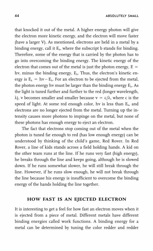
44 ABSOLUTELY SMALL
that knocked it out of the metal. A higher energy photon will give
the electron more kinetic energy, and the electron will move faster
(have a larger V). As mentioned, electrons are held in a metal by a
binding energy, call it Eb, where the subscript b stands for binding.
Therefore, some of the energy that is carried by the photon has to
go into overcoming the binding energy. The kinetic energy of the
electron that comes out of the metal is just the photon energy, E �
hν, minus the binding energy, Eb. Thus, the electron’s kinetic en-
ergy is Ek � hν�Eb. For an electron to be ejected from the metal,
the photon energy hν must be larger than the binding energy Eb. As
the light is tuned further and further to the red (longer wavelength,
λ), ν becomes smaller and smaller because ν � c/λ, where c is the
speed of light. At some red enough color, hν is less than Eb, and
electrons are no longer ejected from the metal. Turning up the in-tensity causes more photons to impinge on the metal, but none of
these photons has enough energy to eject an electron.
The fact that electrons stop coming out of the metal when the
photon is tuned far enough to red (has low enough energy) can be
understood by thinking of the child’s game, Red Rover. In Red
Rover, a line of kids stands across a field holding hands. A kid on
the other team runs at the line. If he runs very fast (high energy),he breaks through the line and keeps going, although he is slowed
down. If he runs somewhat slower, he will still break through the
line. However, if he runs slow enough, he will not break through
the line because his energy is insufficient to overcome the binding
energy of the hands holding the line together.
HOW FAST IS AN EJECTED ELECTRON
It is interesting to get a feel for how fast an electron moves when it
is ejected from a piece of metal. Different metals have different
binding energies called work functions. A binding energy for a
metal can be determined by tuning the color redder and redder

THE PHOTOELECTRIC EFFECT AND EINSTEIN’S EXPLANATION 45
and seeing the wavelength of light at which photons cannot eject
electrons. For a metal with a small binding energy, a typical cutoff
wavelength for electron ejection is 800 nm. For λ � 800 nm, ν �
3.75 � 1014 Hz, and Eb � hν � 2.48 � 10�19 J. If we shine green
light on the metal with a wavelength of 525 nm, the energy of the
photon is 3.77 � 10�19 J. The kinetic energy of the electron that will
be ejected from the metal is Ek � hν�Eb � 1.30 � 10�19 J. We can
find out how fast the electron is moving using Ek �12meV2 � 1.30
� 10�19 J, where me is the electron mass, me � 9.11 � 10�31 kg
(kg is kilograms, that is, 1000 grams). Multiplying the equation for
Ek by 2 and dividing by me gives V2 � 2(1.30 � 10�19 J)/me � (2.60
� 10�19 J)/(9.11 � 10�31 kg) � 2.85 � 1011 m2/s2. This value is the
square of the velocity. Taking the square root, V � 5.34 � 105 m/
s, which is about one million miles per hour. In this example of thephotoelectric effect, the ejected electrons are really moving.
Classical electromagnetic theory describing light as waves
seems to work perfectly in describing a vast array of phenomena
including interference, but it can’t come close to explaining the pho-
toelectric effect. Einstein explains the photoelectric effect, but now
light can’t be waves, so what happens to the classical description of
interference? Reconciling the photoelectric effect and interferencebrings us to the cusp of quantum theory and back to Schrodinger’s
Cats.

5
Light:
Waves or Particles?
THE EXPLANATION OF THE photoelectric effect discussed in Chapter 4
required a new theoretical description of the interferometer experi-
ment discussed in connection with Figure 3.4. Understanding the
interferometer experiment in a manner that does not contradict the
description of the photoelectric effect requires the big leap into
thinking quantum mechanically rather than thinking classically. Indiscussing absolute size in Chapter 2, the idea was introduced that
for a system that is small in an absolute sense, a measurement will
make an unavoidable nonnegligible disturbance. However, we did
not discuss the nature or consequences of such a disturbance. Now,
we need to come to grips with the true character of matter and what
happens when we make measurements.
The problem we have is that light waves were used to explainthe interference phenomenon in Figure 3.4, but ‘‘particles of light,’’
quanta called photons, were used to explain the photoelectric effect
in connection with Figures 4.3 and 4.4. The classical mathematical
description of light waves employed Maxwell’s equations to quanti-
tatively describe interference. The mathematical entity that repre-
46

LIGHT: WAVES OR PARTICLES? 47
sented a light wave in the theory is called a wavefunction. A
function gives a mathematical description of something, in this case
a light wave. It describes the amplitude, frequency, and the spatial
location of a light wave. The incoming light wave is described by a
single wavefunction. In the classical description, after the light wave
hits the 50% beam splitter, half of the wave goes into each leg of
the interferometer (see Figure 3.4). There are now two waves andtwo wavefunctions, one for each wave. These wavefunctions de-
scribe waves that are each half of the intensity of the original incom-
ing wave and are in different locations, the two legs of the
interferometer. When these two wavefunctions are combined math-
ematically to describe the nature of the overlap region inside the
circle in Figure 3.4, the interference pattern can be calculated. All
of this worked so well that it was thought that the same math mustapply to photons.
CLASSICAL DESCRIPTION OF INTERFERENCEDOESN’T WORK FOR PHOTONS
Figure 5.1 shows the interferometer again with everything exactly
the same as in Figure 3.4 except that the incoming light beam isnow composed of photons. Initially, it was thought that when the
beam of photons hits the 50% beam splitter, half of the photons go
into leg 1 of the apparatus and head toward end mirror 1, while the
other half of the photons go into leg 2 of the apparatus and head for
end mirror 2. The photons would then reflect from the end mirrors
and after again hitting the beam splitter, half of the photons from
each leg would cross in the overlap region. The inference patternwas thought to develop when photons from one leg of the apparatus
interfered with photons from the other leg of the apparatus. This
thinking proved to be incorrect.
To describe the interference effect, the mathematical formula-
tion in terms of Maxwell’s wavefunctions was not changed at all.
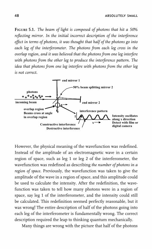
48 ABSOLUTELY SMALL
FIGURE 5.1. The beam of light is composed of photons that hit a 50%
reflecting mirror. In the initial incorrect description of the interference
effect in terms of photons, it was thought that half of the photons go into
each leg of the interferometer. The photons from each leg cross in the
overlap region, and it was believed that the photons from one leg interfere
with photons from the other leg to produce the interference pattern. The
idea that photons from one leg interfere with photons from the other leg
is not correct.
Intensity oscillatesalong x directionDetect with film ordigital camera
I
interference pattern
x
overlap regionBeams cross at angle in overlap region
Constructive interferenceDestructive interference
xxincoming beam
end mirror 1
50% beam splitting mirror 2
end mirror 2
photons
However, the physical meaning of the wavefunction was redefined.Instead of the amplitude of an electromagnetic wave in a certain
region of space, such as leg 1 or leg 2 of the interferometer, the
wavefunction was redefined as describing the number of photons in a
region of space. Previously, the wavefunction was taken to give theamplitude of the wave in a region of space, and this amplitude couldbe used to calculate the intensity. After the redefinition, the wave-function was taken to tell how many photons were in a region ofspace, say leg 1 of the interferometer, and the intensity could stillbe calculated. This redefinition seemed perfectly reasonable, but itwas wrong! The entire description of half of the photons going intoeach leg of the interferometer is fundamentally wrong. The correctdescription required the leap to thinking quantum mechanically.
Many things are wrong with the picture that half of the photons

LIGHT: WAVES OR PARTICLES? 49
go into each leg of the interferometer and then come together and
interfere with each other. The simplest experiment that shows the
problem with this description is the intensity dependence of the
interference pattern (the lower right portion of Figure 5.1). The
shape of the interference pattern observed in the overlap region of
the interferometer is independent of the intensity used to create it.
For a given method of detection, a piece of photographic film or adigital camera, note that if the intensity is turned up it will take less
time to acquire a high-quality pattern, but the shape of the pattern
is unchanged. That is, the separation and shapes of the peaks and
nulls in the pattern are unchanged. As discussed in Chapter 3, the
periodicity of the pattern depends on the crossing angle of the
beams and the wavelength of light. It does not depend on the inten-
sity. If the intensity is reduced, it will take more time to collect thepattern, but the pattern will not change shape. A standard red laser
pointer puts out 1 mW (milliwatt), which is one thousandth of a
watt, or 0.001 J/s (joules per second). The red color is approximately
650 nm, that is, the wavelength λ � 650 nm. Using λν � c and E
� hν where h is Planck’s constant, ν is the frequency of the light,
and c is the speed of light, one photon of 650 nm light is about 3
� 10�19 J. So the 1 mW laser pointer is emitting about 3 � 1015
photons per second, that is 3 thousand trillion photons per second.
If this is the input beam for the interferometer, the interference
pattern will be very easy to record and, in fact, if the fringe spacing
is big enough (see Chapter 3, the discussion of fringe spacing fol-
lowing Figure 3.4), you will be able to see the interference pattern
with your eyes.
Imagine turning the intensity down and down. Soon, you willnot be able to see the interference pattern because your eyes are
not very sensitive light detectors, but you can still record it with
photographic film or a digital camera. Once recorded, the pattern is
the same. Turn the intensity down a factor of 3000 to a trillion
photons a second, and the pattern is unchanged. In the description

50 ABSOLUTELY SMALL
in which half of the photons go into each leg of the apparatus, half
a trillion photons per second go into each leg of the interferometer.
Turn down the intensity to a billion photons per second, and the
pattern is the same. Further reduce the intensity to a million pho-
tons per second, and there is still no change. Here is where the
fallacy in the description becomes obvious. Turn down the intensity
until there is only one photon per second entering the apparatus.Again, the pattern is unchanged. At one photon per second, it will
take a long time to record enough signal to see the interference
pattern, but if you wait long enough the pattern is the same.
When only one photon per second is entering the interferome-
ter, there is only one photon at a time in the apparatus. A photon
will take on the order of one hundred millionth of a second (10�8 s)
to traverse the interferometer. With one photon per second, there isvirtually no chance that there is more than one photon at a time in
the instrument, yet the interference pattern, once recorded, is the
same. But the modified classical description of the interference ef-
fect in terms of photons said that half of the photons go into leg 1
and half of the photons go into leg 2. The photons in leg 1 interfere
with the photons in leg 2 to produce the interference pattern. If
there is only one photon in the apparatus at a time, there is no otherphoton for it to interfere with. The ‘‘half of the photons go into each
leg of the apparatus model’’ predicts that the interference pattern
should vanish at low enough intensity. The interference pattern
does not disappear at low intensity. The model is wrong!
A NEW DESCRIPTION OF PHOTONSIN THE INTERFEROMETER
Here is where the complete change in thinking is required that will
bring us back to Schrodinger’s Cats. How is it possible to have an
interference pattern when only one photon enters the interferome-
ter at a time? Our understanding of this problem and the nature of

LIGHT: WAVES OR PARTICLES? 51
quantum mechanics in general is based on the conceptual interpre-
tation of the mathematical formalism that is strongly associated
with the work of Max Born (1882–1970). Born won the Nobel Prize
in Physics in 1954 ‘‘for his fundamental research in quantum
mechanics, especially for his statistical interpretation of the wave-
function.’’ This interpretation is frequently referred to as the Copen-
hagen interpretation.The correct description of the interferometer experiment is
that each photon goes into both legs of the interferometer. This is the
big leap. A single photon encounters the 50% beam splitter. That
means there is a 50% chance that the photon will be reflected and
go into leg 1 of the interferometer (see Figure 5.1) and a 50%
chance it will go into leg 2. Classically one would say the photon
must go one way or the other, that is, it either goes into leg 1 or itgoes into leg 2. This is not correct. When the photon encounters
the beam splitter, its state is changed. If a photon is in fact moving
in leg 1, call this state of motion ‘‘translation state 1,’’ abbreviated
T1. If a photon is moving in leg 2, call this state of motion ‘‘trans-
lation state 2,’’ abbreviated T2. After a photon interacts with the
beam splitter, it is not in T1 or T2. The state of the system after
the beam splitter is referred to as a superposition state. It is anequal mixture of T1 and T2. In some sense, the photon is simulta-
neously in both T1 and T2. This sounds really strange. The single
photon is in two regions of space simultaneously. It is in a super-
position translation state T � T1 � T2. It is in a state that is an
equal mixture of T1 and T2.
The photon is in the superposition translation state T � T1 �
T2 because this is what is known about it. It has a 50% chance ofbeing in leg 1 (T1) and a 50% chance of being in leg 2 (T2). The
Born interpretation of the wavefunction states that the wave is not
a real wave in the sense of the amplitude of an oscillating electro-
magnetic field. Rather, the wavefunction describes a ‘‘probability
amplitude wave.’’ The incorrect interpretation of the wavefunction in
52 ABSOLUTELY SMALL
terms of photons is that it tells how many photons are in each leg
of the apparatus, that is, how many photons are in a region of space.
The correct interpretation is that the wavefunction is related to the
probability of finding a photon in a region of space. The difference
between the incorrect and correct interpretation may not seem like
a major difference, but, as shown in detail below, it is a fundamen-
tal change in our view of nature. In the classical description of light,
the intensity is proportional to the absolute value squared of the
amplitude of the electric field, which in turn was given by the ampli-
tude of the wavefunction. In the Born interpretation, the absolute
value squared of the wavefunction for a certain region of space gives
the probability of finding a particle, in this case a photon, in that
region of space.
A PHOTON INTERFERES WITH ITSELF
When the photon meets the beam splitter, two probability ampli-
tude waves are created, one in leg 1 and one in leg 2. The total
probability amplitude wave T is the superposition of the probability
amplitude waves T1 and T2. After encountering the beam splitter,
each and every photon is in a state T1 � T2. Because there are two
probability amplitude waves after the beam splitter, they cross in
the overlap region. A single photon inside the interferometer has
two waves, T1 and T2, associated with it. The interference of these
two waves determines the probability of finding a photon near the
peak, which is high, and finding a photon near the null, which is
low. A photon interferes with itself because it is composed of two
waves in the interferometer, and two waves can interfere with each
other. Because every single photon is placed in the T1 � T2 super-
position state after meeting the beam splitter, there is no problem
with turning down the intensity. A single photon entering the appa-
ratus produces two waves, probability amplitude waves, in the inter-

LIGHT: WAVES OR PARTICLES? 53
ferometer. Therefore, there is always a pair of waves to produce an
interference pattern.
A PHOTON CAN BE IN TWO PLACES AT ONCE
The first natural response of a classical thinker to the Born interpre-
tation is ‘‘this is nuts.’’ Are we really to believe that a single photoncan be in two places at once? After meeting the beam splitter, the
state that is produced is T1 � T2. The state T1 � T2 means that in
some sense the photon is simultaneously in both legs of the appara-
tus. If this is true, why don’t we just make some measurements to
see where the photon is? It doesn’t do much good to make the
measurement with trillions of photons going into the apparatus. If
we put an instrument in leg 1 to see how much light there is, wewill find half of the light. However, that doesn’t tell us what we want
to know. Maybe half of the photons go in each leg and we see half,
or maybe there is a 50% chance that each photon goes into each leg.
We will still see half. The correct experiment is to use such low-
intensity light so that only one photon is in the apparatus at a time.
Consider the experiment in which we shoot one photon at a
time into the interferometer. We use a photodetector that is so sen-sitive that it can detect a single photon. This is readily doable with
the scientific equivalent of a superdigital camera. We place the de-
tector in leg 1 of the interferometer. A photon enters the apparatus,
and we detect it. We see an entire photon. We don’t see half a pho-
ton. Another photon goes in the apparatus, and we don’t see a pho-
ton. Five more photons enter the apparatus. We detect two of them
and do not detect the other three. After doing this for a long time,it is found that 50% of the photons are observed by the detector
placed in leg 1 of the apparatus. We also find that no interference
pattern was produced. In fact, what is observed is a single bright
spot (no oscillatory pattern) in the region in which the interference
pattern occurred previously.

54 ABSOLUTELY SMALL
Observation Causes a Nonnegligible Disturbance Causing aChange of State
What is going on? After the photon meets the beam splitter, it is in
a superposition state, T1 � T2. However, photons are particles that
are small in the absolute sense. The act of making an observation
causes a nonnegligible disturbance. When we place the photodetec-
tor in leg 1 of the apparatus, we are making an observation of the
location of the photon. The act of making the observation causes
the system to jump from being in the superposition state T1 � T2
into either a pure state T1 or a pure state T2. The superposition
wavefunction has been ‘‘collapsed’’ into one of the pure states that
make up the superposition. If the system makes the jump into the
state T1, the photon is detected. Of course, once it slams into the
photodetector, it does not continue to propagate through the inter-
ferometer. If the photon jumps into the state T2, it is not detected
with the photodetector that is located in leg 1, and it continues to
propagate, eventually reaching the region in which the instrumenta-
tion is set up to observe the interference pattern. However, because
the photon is in the pure state T2, there is only a single probability
amplitude wave. When it reaches the ‘‘overlap’’ region (see the bot-
tom of Figure 5.1), there is no other probability amplitude wave to
interfere with. Therefore, no interference pattern is created. A sin-
gle spot is formed as each photon that traverses the apparatus in
the pure T2 state hits a single spot on the detector like a bullet
aimed at that spot. The spot has the same size (diameter) as the
initial light beam that entered the apparatus, but no spatially oscilla-
tory interference pattern.
BACK TO SCHRODINGER’S CATS
Making the observation of the location of the photon with the photo-
detector in leg 1 of the interferometer causes the photon to jump

LIGHT: WAVES OR PARTICLES? 55
from the mixed superposition state T1 � T2 into a pure state, either
T1 or T2. However, on a single measurement it is not possible to
know which state will be produced by the observation. The chance
is 50/50 that it is in T1 and 50/50 that it is in T2. After many mea-
surements, we know that the probability of making the jump to T1
is 50%, but it is impossible to say in advance what will happen for
any single observation. This is a true physical manifestation of theissues raised with Schrodinger’s Cats in Chapter 1, where we had
1000 boxes with a cat in each one. Each cat was in a superposition
state that was 50% alive and 50% dead. In this very nonphysical
heuristic scenario, when a box is opened an observation is made as
to the health of the cat. Sometimes the cat is perfectly healthy and
sometimes the cat is dead. After opening all of the boxes, it was
determined that the probability of finding a live cat was 50%, butthere is no way of predicting ahead of time when opening a particu-
lar box, that is, on making a single observation, whether a live or
dead cat will be found. Before opening the box, the cat is in a super-
position state that is a 50/50 mixture of live and dead. The act of
making the observation makes a nonnegligible disturbance and
causes the superposition state to jump into either a pure live state
or a pure dead state. As discussed in Chapter 1, a live/dead catsuperposition state does not and cannot exist, but the interferome-
ter is a real example of the ideas illustrated by Schrodinger’s Cats.
A photon can easily be placed into a superposition state consist-
ing of a 50/50 mixture of two translations states using the 50%
beam splitter. When it is in the superposition state, it is not possible
to say whether the photon is in leg 1 or leg 2 of the apparatus. It is
only possible to say that if we make a measurement to see wherethe photon is, the measurement will make a nonnegligible distur-
bance. The disturbance will cause the state of the system to change
from having equal probability of being in the two legs of the inter-
ferometer to being in either one or the other. The interference pat-
tern is produced when the photon’s probability amplitude waves

56 ABSOLUTELY SMALL
interfere with each other. The two pieces of the superposition state,
T1 and T2, which comprise the total probability amplitude wave
for a photon in the interferometer, interfere with each other. If an
observation is made to see where the photon is, it will be found to
be either in leg 1 or leg 2 of the apparatus. However, the act of
observation changes the system so that it is no longer in a superpo-
sition state. There are no longer two parts of the probability ampli-tude wave to interfere with each other, and the interference pattern
vanishes. Thus, a photon in an interferometer is a real manifesta-
tion of the ideas relating to Schrodinger’s Cats.
BACK TO THE PHOTOELECTRIC EFFECT
In Chapter 4, the photoelectric effect was described in terms of pho-tons, which are particles that behave in some sense like bullets of
light. One photon strikes one electron and knocks it out of a piece
of metal (see Figure 4.3). The description of the photoelectric effect
showed that the classical description of light as an electromagnetic
wave was incorrect. A new concept had to be introduced to explain
both the photoelectric effect and the fact that photons could produce
an interference pattern. The Born interpretation of the wavefunc-tion as a probability amplitude wave gave the photon the necessary
wavelike characteristics, so that photons could produce an interfer-
ence pattern. However, in discussing the probability amplitude
waves in connection with the interferometer, we only considered
the location of the photon in terms of two rather large regions of
space; a photon was in a superposition state, T1 � T2, with equal
probabilities of being in leg 1 and leg 2 of the interferometer. Thephotoelectric effect implied that a photon is quite small. Chapter 6
will show how a superposition of probability amplitude waves can
produce a photon that is very small in size. The ideas will lead to
one of the central and most nonclassical aspects of quantum me-
chanics, the Heisenberg Uncertainty Principle.
6
How Big Is a Photon
and the Heisenberg
Uncertainty Principle
IN CHAPTER 5, WE LEARNED that a photon in an interferometer inter-
feres with itself. In some sense, a photon can be in more than one
place at a time. The photon location is described as a probability
amplitude wave. This is not like a water wave, a sound wave, or even
a classical electromagnetic wave. The wave associated with a photon
(or other particles like electrons) describes the probability of findingthe particle in some region of space. In the interferometer problem
(Figures 3.4 and 5.1), a single photon was in leg 1 and leg 2 simulta-
neously, with equal probability of finding the photon in either of
these regions of space. To understand and describe the location of
a photon in more detail, it is necessary to discuss more aspects of
waves. We need to know about the nature of the probability ampli-
tude waves, particularly how they combine and what happens whena measurement is made.
The simplest problem to discuss is a free particle, which was
introduced in Chapter 2. A free particle could be a photon, an elec-
tron, or a baseball. It is a free particle if no forces are acting on it.
That is, there is no gravity, no electric or magnetic fields, no photons
57

58 ABSOLUTELY SMALL
hitting an electron, no baseball bats hitting the baseball, no air resis-
tance, and so on. With no forces acting on a particle, it has a perfectly
defined and unchanging momentum. Thus, if it is moving in a par-
ticular direction, it will just keep going in that direction. We can call
that direction anything we want, so let’s call it the x direction. Think
of a graph with the horizontal axis x. We will just pick the direction
of the x axis to be along the direction the particle is moving. In con-nection with Figure 2.5, we talked about a classical particle moving
along x with a classical momentum p. Here we want to discuss the
nature of a quantum particle with momentum p.
PARTICLES HAVE WAVELENGTHS
For a photon, the momentum is given as p � h/λ, where h is Plan-ck’s constant and λ is the wavelength of the light. Therefore, the
momentum is related to the wavelength (the color) of the light.
Prince Louis-Victor Pierre Raymond de Broglie (1892–1987) won
the Nobel Prize in Physics in 1929 ‘‘for his discovery of the wave
nature of electrons.’’ De Broglie showed theoretically that particles,
such as electrons or baseballs, also have a wave description. As dis-
cussed below, the wave description of electrons—or any type of par-ticle—is in terms of the same types of waves as a photon, probability
amplitude waves, as introduced in Chapter 5.
The wavelength associated with a particle is λ � h/p. This is a
simple rearrangement of the formula for the photon momentum
given above. If both sides of the photon momentum formula are
multiplied by λ and divided by p, then the expression for the wave-
length associated with a particle is obtained. De Broglie’s importantresult is that the relationship between the momentum and the
wavelength is the same for photons (light) as it is for material parti-
cles, such as electrons and baseballs. Therefore, the properties of
photons are described in fundamentally the same way as the proper-
ties of electrons, as well as baseballs. The wavelength associated

HOW BIG IS A PHOTON 59
with a particle is called the de Broglie wavelength. (We will see with
physical examples in the next chapter why baseballs don’t seem to
have wavelike properties, but photons and electrons do.)
WHAT A FREE PARTICLE WAVEFUNCTIONLOOKS LIKE
For a free particle with some particular value of its momentum, p,
what does the wavefunction look like? Recall that the wavefunction
is related to the probability of finding the particle someplace in
space. Figure 6.1 shows a graph of the wavefunction for a free parti-
cle with the momentum, p. As discussed above, the wavelength of
the wavefunction associated with the particle is λ � h/p. As can be
seen in the figure, the wavefunction for a free particle is represented
by two waves called the real and the imaginary parts of the wavefunc-
tion. These components are equivalent. The term imaginary is a
FIGURE 6.1. The wavefunction for a free particle with momentum p,
which has wavelength, λ � h/p. A quantum mechanical wavefunction
can have two parts, called real and imaginary. Both waves have the same
wavelength. They are just shifted by one-fourth of a wavelength, which is
the same as a 90� shift in the phase. These two components are separate
from each other. They do not interfere either constructively or destruc-
tively. For a free particle with the well-defined value of the momentum,
p, the wave function extends from positive infinity to negative infinity,
�� to ��.
real imaginary

60 ABSOLUTELY SMALL
mathematical term. It does not imply that in some sense the imagi-
nary component is less important than the part referred to as real.
It is just jargon to identify the two components, although they do
have differences in the way they are represented mathematically.
The real and the imaginary components of the wavefunction have
the same wavelength, but are shifted by one-fourth of the wave-
length. That means that one wave is shifted in phase relative to theother by 90�. The two components of the wavefunction do not inter-
fere with each other, either constructively or destructively, because
in a mathematical sense and in essence they are perpendicular to
each other.
A PARTICLE WITH WELL-DEFINED MOMENTUMIS SPREAD OVER ALL SPACE
The important feature of the wavefunction shown in Figure 6.1 is
that it extends from positive infinity to negative infinity, that is,
from �� to ��. In Figure 6.1, only a small section of the wavefunc-
tion in a small region of space is shown because we cannot plot ��
to �� on a finite piece of paper. The wave shown in the figure just
keeps going to the right and to the left. It is uniform across allspace. This means that for a quantum mechanical particle with a
definite value of the momentum, p, we are equally likely to find the
particle anywhere along the x axis, the horizontal axis in the graph.
The vertical axis tells the probability amplitude of finding the parti-
cle somewhere. Both the real (dashed) and imaginary (solid) compo-
nents oscillate positive and negative. Both have places where they
are zero.The fact that the wavefunction oscillates positive and negative
doesn’t matter. In explaining photon interference quantum me-
chanically following Figure 5.1, the Born interpretation of the wave-
function was introduced. In the Born interpretation, the absolute
value squared of the wavefunction in a certain region of space gives

HOW BIG IS A PHOTON 61
the probability of finding a particle in that region of space. When
the wavefunction is squared, it becomes only positive in the same
way that 22 � 4 and (�2)2 � 4 because minus times a minus is a
plus. Note that in Figure 6.1, whenever one wave is zero, the other
wave is either at a positive or negative maximum. Where one wave
is small, the other wave is big. When the wavefunction is analyzed
mathematically, and as can be seen from the graph, at all locationsthe absolute value squared of the wavefunction is uniform along the
x axis.
The absolute value squared of the wavefunction for a free parti-
cle is uniform along the x axis from �� to ��. Therefore, the
probability of finding the particle anywhere in space is uniform.
The particle has equal probability of being found at x � 10, or x �
�1,000,000, or anywhere else. Imagine that you are a tiny creature,frequently referred to as Maxwell’s Demon. You are standing next
to the particle-wave shown in Figure 6.1. You make a grab for the
particle. There is some probability that you will find it in your hand.
If you start over and do this again and again, depending on the size
of your hand, you may eventually come up with the particle. Each
time you need to start fresh in your attempt to grab the particle. If
you move somewhere else along the wave and do the same thing,the chance that you will come up with the particle is no different.
This is what it means to say that there is equal probability for find-
ing the particle anywhere. There is no best spot for Maxwell’s
Demon to stand to try to grab the particle. All locations are equally
good.
This picture of a free particle described by a wavefunction that
represents equal probability of finding the particle anywhere doesn’tgo along very well with our classical concept of a particle. In Figure
2.5, we described a classical particle as having a particular momen-
tum and position at a given time. In discussing the photoelectric
effect (Figure 4.3), Einstein described light as photons, which are
quanta of light. One photon ‘‘hits’’ one electron, and the electron

62 ABSOLUTELY SMALL
flies out of the piece of metal. This description almost sounds like
both the photon and the electron are particles in the classical me-
chanics sense of particles. However, in discussing the interference
of photons in conjunction with Figure 5.1, it was necessary to use
the Born interpretation and describe photons as probability ampli-
tude waves, with half of the probability going into each leg of the
interferometer. In Figure 6.1, the plot of a free particle wavefunc-tion is completely delocalized, spread out over all space. The de-
scription is the same for a photon or an electron.
INTERFERENCE OF WAVES WITHDIFFERENT WAVELENGTHS
So what are photons and electrons and rocks and anything else? Arethey particles or waves? To see that there is no contradiction in the
quantum mechanical description of the nature of things, we need
to discuss waves and the interference of waves further. In connec-
tion with Figures 3.2 and 3.3, we discussed that waves could inter-
fere constructively to give a bigger wave or destructively to give a
smaller wave or no wave at all. In the examples in Figures 3.2 and
3.3, the waves have the same wavelengths. When they added con-structively (Figure 3.2), all of the positive peaks lined up with the
positive peaks and the negative peaks lined up with the negative
peaks to give increased amplitude. When the waves added destruc-
tively (Figure 3.3), the positive peaks lined up with the negative
peaks and vice versa, to give cancellation. However, waves of differ-
ent wavelengths can also interfere.
Figure 6.2 shows a plot of five waves with different wave-lengths. The units of length do not matter. What is important is
that the five waves have wavelengths, λ � 1.2, 1.1, 1.0, 0.9, and 0.8.
The phase of the waves are adjusted so that they all match at the
point x � 0, where x is the horizontal axis. The waves match at x �
0 in the sense that each wave has a positive going peak at x � 0.

HOW BIG IS A PHOTON 63
FIGURE 6.2. Five waves are shown that have different wavelengths. The
wavelengths are λ � 1.2, 1.1, 1.0, 0.9, and 0.8. The phases are adjusted
so all of the peaks of the waves match at 0 on the horizontal axis. How-
ever, because the waves have different wavelengths, they do not match up
at other positions, in contrast to Figure 3.2. Note that at a position of
approximately 10 or�10, the dark gray wave has a positive peak, but
the dashed light gray wave has a negative peak.
–20
1
0
–1–10 0 10 20
However, because the waves have different wavelengths, the peaksdo not necessarily match at other points along the x axis. For exam-ple, at about x � 10 or �10, the dark gray wave has a maximumbut the dashed light gray wave has a minimum. In addition, at ap-proximately 10, one wave has a negative value and another has apositive value. At approximately x � 16 or �16, two waves havemaxima, but another wave is at a minimum. The important pointis that for waves with different wavelengths, at one point (x � 0 inthe example), all of the waves can be matched, but in general, atother points, some of the waves will be positive and some of thewaves will be negative.
Figure 6.3 shows the result of superimposing (adding up) thefive waves in Figure 6.2. At x � 0 (horizontal axis) in Figure 6.2, allof the waves are exactly in phase. The superposition (adding thewaves together) shown in Figure 6.3 yields a maximum. In Figure6.2, the waves are all exactly in phase only at x � 0. Near x � 0, thedifference in the wavelengths has not produced a large shift in the

64 ABSOLUTELY SMALL
peaks of one wave relative to another, so the waves are still pretty
much in phase. There is another set of maxima at about x � 6 and
�6. However, these maxima are not as large as the one at x � 0,
because the peaks of the waves are not all right on top of each other,
as can be seen in Figure 6.2. Beyond x � �10, the amplitude of
the superposition is getting small. At any point, some waves are
positive and some waves are negative, and they tend to destructivelyinterfere. Because there are only five waves, the destructive interfer-
ence is only partial.
Figure 6.4 shows the superposition of 250 waves with different
wavelengths. The waves have equal-sized steps in wavelength in the
range of wavelengths from 0 to 4. As for the five waves and their
superposition shown in Figures 6.2 and 6.3, each wave has the same
amplitude. The phases of the 250 waves are adjusted to match at x
FIGURE 6.3. The superposition of the five waves shown in Figure 6.2. At
x � 0 (horizontal axis), all of the waves in figure 6.2 are in phase, so
they add constructively. Near x � 0, the waves are still pretty much in
phase, but the next set of maxima at about x � 6 and �6 are not as
large as the maximum at x � 0. In the regions between 10 and 20 and
�10 and �20, the difference in wavelengths makes some of the waves
positive, where others are negative. There is significant cancellation.
–20 –10 10 20
-4
-2
2
4

HOW BIG IS A PHOTON 65
FIGURE 6.4. The superimposition of 250 waves with equally spaced
wavelengths spanning the wavelength range 0 to 4. Compared to Figure
6.3, which is the superposition of five waves, this superposition has a
much larger peak at x � 0, the region of maximum constructive interfer-
ence, and destructive interference reduces the other regions more. The
amplitude of the superposition is dying out going toward �20.
250
150
50
–50
–20 –10 2010
� 0 (x is the horizontal axis). Because there are many more waves
over a wider range of wavelengths than in the superposition shown
in Figure 6.3, the peak around x � 0 is much narrower, and therest of the superposition dies out much more rapidly. The little os-
cillations come from the fact that all of the waves in the superposit-
ion have the same amplitude. If the amplitude of the wave at the
middle of the spread of wavelengths has the biggest amplitude and
the amplitudes of the other waves get smaller and smaller for wave-
lengths further and further from the center wavelength, it is possi-
ble to create a superposition that decays smoothly to zero withoutthe set of deceasing amplitude oscillations. This type of superposit-
ion will be discussed below.
THE SUPERPOSITION PRINCIPLE
In Chapter 5, the interference experiment was analyzed in terms of
the superposition of two photon translation states, T1 and T2. A

66 ABSOLUTELY SMALL
photon in the interferometer is described as being in the 50/50 su-
perposition state, T � T1 � T2. The idea of superposition is central
to the quantum theoretical description of nature; it is called the
Superposition Principle and assumes that ‘‘Whenever a system is
in one state, it can always be considered to be partly in each of two
or more states.’’
An original state can be regarded as a superposition of two or
more states, as in the interference problem in which the translation
state T of the photon was described as a superposition of T1 and
T2. Conversely, two or more states can be superimposed to make a
new state. It is this second statement that we will now use to under-
stand the fundamental nature of particles. The fact that a photon
can act like a particle in the photoelectric effect but act like a wave
to give rise to the interference effect follows from the superposition
principle and leads to the Heisenberg Uncertainty Principle.
Eigenstates
In connection with Figure 6.1, it was stated that a free particle with
perfectly defined momentum p is a delocalized probability ampli-
tude wave spread out over all space. If a particle exists in such a
state, it is said to be in a momentum eigenstate. In discussing the
interference problem, we called T1 and T2 pure states, but the cor-
rect name for them is eigenstates. Eigen is German for characteris-
tic, so an eigenstate is a characteristic state. An eigenstate for a
particular observable property, such as momentum, is a state with
a perfectly defined value of that property. The momentum eigen-
states of a free particle are delocalized over all space. One such eigen-
state exists for each of the infinite number of possible values of the
momentum. Each of these momentum eigenstates is associated
with an exact value of momentum of the particle. The particle’s
location is uniform over all space because the wavefunction associ-
ated with the eigenstate is spread out over all space. However, the

HOW BIG IS A PHOTON 67
Superposition Principle tells us that we can superimpose any num-
ber of momentum eigenstates to make a new state.
Superposition of Momentum Eigenstate ProbabilityAmplitude Waves
To understand the nature of real particles, photons, electrons, and
so on, we will superimpose a range of momentum eigenstate proba-
bility amplitude waves, such as the one shown in Figure 6.1. For
each momentum p, the wave has a different wavelength, λ � h/p.
In Figures 6.3 and 6.4, we saw that adding together waves of differ-
ent wavelengths concentrated the amplitude of the wave in a parti-
cular region. As mentioned in both examples above, the amplitude
of each wave in the superposition was the same. Now we will super-
impose momentum probability amplitude waves with different am-
plitudes. There is one wave (a particular value of p) with the largest
amplitude. The other waves with different wavelengths have ampli-
tudes that decrease as the wavelength becomes greater than or less
than the wavelength of the wave with the maximum amplitude. So,
we have a distribution of wavelengths centered around the wave-
length of the maximum amplitude wave. The wavelength with maxi-
mum amplitude is at the center of the distribution. By a
distribution, we just mean that there is a range of wavelengths, in
the same way that if you have a room full of people there will be a
distribution of ages. There will be some people of average age, the
center of the distribution, and some people older than the average
and some people younger. Here, we have a wave at the center of the
distribution with other waves having shorter wavelengths and still
others having longer wavelengths.
Figure 6.5 illustrates a distribution of momentum probability
amplitude waves. p0 is the momentum of the wave at the center of
the distribution of waves. It has a wavelength λ � h/p0. It is the
wave with the biggest amplitude, that is, the biggest probability of
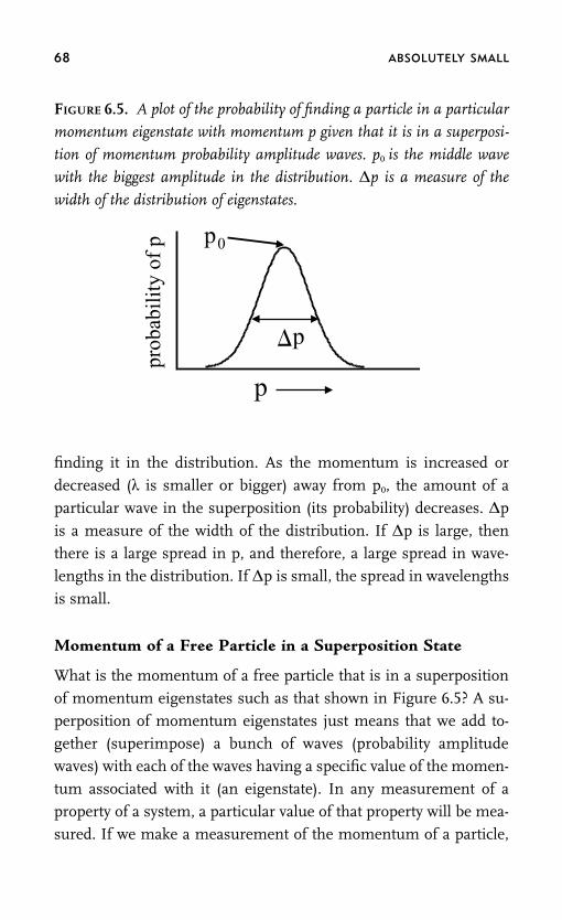
68 ABSOLUTELY SMALL
FIGURE 6.5. A plot of the probability of finding a particle in a particular
momentum eigenstate with momentum p given that it is in a superposi-
tion of momentum probability amplitude waves. p0 is the middle wave
with the biggest amplitude in the distribution. Δp is a measure of the
width of the distribution of eigenstates.
p
�
p0
prob
abili
ty o
f p
p
finding it in the distribution. As the momentum is increased or
decreased (λ is smaller or bigger) away from p0, the amount of a
particular wave in the superposition (its probability) decreases. Δp
is a measure of the width of the distribution. If Δp is large, then
there is a large spread in p, and therefore, a large spread in wave-
lengths in the distribution. If Δp is small, the spread in wavelengths
is small.
Momentum of a Free Particle in a Superposition State
What is the momentum of a free particle that is in a superposition
of momentum eigenstates such as that shown in Figure 6.5? A su-
perposition of momentum eigenstates just means that we add to-gether (superimpose) a bunch of waves (probability amplitude
waves) with each of the waves having a specific value of the momen-
tum associated with it (an eigenstate). In any measurement of a
property of a system, a particular value of that property will be mea-
sured. If we make a measurement of the momentum of a particle,

HOW BIG IS A PHOTON 69
we will measure a single value of the momentum. The nature of the
disturbance that accompanies the measurement of an absolutely
small object is to collapse the superposition state into a single eigen-
state. Making a measurement changes a system by taking it from
its initial superposition state to one particular eigenstate. This is
what is meant by collapse.
In discussing the interference problem, we said that if we triedto find out if the photon was in the state T1 by placing a detector in
leg 1 of the interferometer, we would destroy the superposition state
necessary for the interference. The superposition state T would
jump into either T1 or T2. Since the state T is a 50/50 superposition
of T1 and T2, half the time a measurement will result in finding the
system in T1 and half the time in T2. On any single measurement,
it is impossible to know ahead of time which result will occur. Manymeasurements show that the superposition is 50/50 because half
the time we find that the photon is in leg 1 of the apparatus (state
T1) and half the time we find the system is in leg 2 of the apparatus
(state T2).
The superposition of momentum eigenstates shown in Figure
6.5 is composed of a vast (infinite) number of states spread over a
range of momenta characterized by the width of the distribution,Δp. Therefore, there is a wide range of momentum values that can
be measured on any single measurement. If we make a single mea-
surement, we will measure one of the many values. Let’s say we
make a measurement and find a momentum a little bigger than p0.
Call it p1 because it is our first measurement. In the process of
making the measurement, we made a nonnegligible disturbance of
the system. It was changed from being in the superposition state toa single eigenstate with momentum p1. So to make another mea-
surement, we need to start over again and prepare the particle (the
system) in the same way we did originally to get the same distribu-
tion of momenta. We make a second measurement. This time we
measure a value that is quite a bit smaller than p0. Call this value

70 ABSOLUTELY SMALL
p2. We prepare the system again, and make another measurement.
We measure p3. Each time we make a measurement on an identi-
cally prepared system, we will measure a particular value of the
momentum. In advance, we don’t know what the value will be. If
we make many, many measurements, we can plot the probability of
measuring particular values of p. Such a plot gives the distribution
like that shown in Figure 6.5. We can’t say what value we will obtain
on a single measurement. However, we do know something. It is
unlikely that we will measure a value of p that is much much greater
or much much smaller than p0 because the distribution has very
low amplitude in the wings (extremes) of the distribution. We are
most likely to measure a value of p that is near p0 because this is
the portion of the distribution where the amplitude is large.
Momentum Not Perfectly Defined for a Particle in aSuperposition of States
A particle in a superposition of momentum eigenstates, such as
that shown in Figure 6.5, does not have a perfectly well-defined
value of the momentum. In a single measurement, we cannot say
what value of the momentum will be measured. We can say we are
most likely to measure a value near p0. With many measurements,
we can determine the probability distribution. A classical particle,
like the one illustrated in Figure 2.5, has a perfectly well-defined
momentum. We can measure it without changing it. If it is a free
particle, we can make many measurements of the momentum at
different times, and we will always measure the same value of p.
This is not the case for an absolutely small quantum particle in a
momentum superposition state. We will measure a single value of
p on a single measurement, but the act of making the measurement
fundamentally changes the nature of the particle. The particle goes
from being in a superposition state to being in an eigenstate (a
single wave with a single value of the momentum). It goes from

HOW BIG IS A PHOTON 71
being in a state in which there is a probability distribution of mo-
menta to a single value of the momentum that is observed. To re-
cover the distribution, the particle needs to be prepared again.
WHERE IS A PARTICLE WHEN IT IS IN AMOMENTUM SUPERPOSITION STATE?
In connection with Figure 6.1, we said that a particle in a single
momentum eigenstate is delocalized over all space. This doesn’t go
along well with the description of the photoelectric effect. Now the
question is where is a particle that is in a momentum superposition
state? We have already hinted at the answer with the discussions
surrounding Figures 6.2 through 6.4. In Figures 6.3 and 6.4, we saw
that a superposition of waves with different wavelengths produced a
spatial distribution that was concentrated in a region of space. In
Figure 6.3, the wavelengths went from 0.8 to 1.2, and the pattern
was not as concentrated as the one in Figure 6.4, which was formed
from wavelengths that went from 0 to 4. Figure 6.6 shows the spa-
tial distribution associated with distribution of waves (momentum
FIGURE 6.6. A plot of the probability of finding the particle at a location
x given that it is in the superposition of momentum eigenstates shown in
Figure 6.5. x0 is the middle position with the greatest probability. Δx is
a measure of the width of the spatial distribution.
x
prob
abili
ty o
f x x0 – average
value of x
�x

72 ABSOLUTELY SMALL
eigenstates) shown in Figure 6.5. There is a position where the
value is maximum, which is also the average value. For larger and
smaller values of x relative to x0, the amplitudes (probabilities) be-
come smaller.
What does the probability distribution of positions (x values)
mean? A particle with the momentum probability distribution
shown in Figure 6.5 gives rise to the spatial probability distribution
shown in Figure 6.6. A single measurement of the position will
measure a particular value of the position. Call it x1. When the posi-
tion measurement is made on the absolutely small quantum parti-
cle, it causes a nonnegligible disturbance that collapses the position
probability distribution into a position eigenstate with a perfectly
defined value of the position. To make another measurement, the
system (a particle) must be prepared again in the identical manner
so that it has the same momentum probability distribution and,
therefore, the same spatial probability distribution. The second
measurement of the particle’s position will give a value, x2, which
in general will not be the same as x1. If the system is prepared again
and again, and many measurements of the position are made, the
position probability distribution shown in Figure 6.6 will be
mapped out. Δx is a measure of the width of the spatial distribution.
The spatial distribution shown in Figure 6.6, which is determined
by many measurements on identically prepared systems, tells the
likelihood of measuring any particular position. A measurement is
more likely to find the particle somewhere in the vicinity of x0, but
on any single measurement, it is impossible to say where the parti-
cle will be found. However, there is only a small probability of mea-
suring a position that is far from x0.
Wave Packets
A particle in a superposition of momentum eigenstates, such as
that shown in Figure 6.5, is called a wave packet. Its momentum

HOW BIG IS A PHOTON 73
is more or less known depending on how big Δp is. Because the
momentum is the mass times the velocity and the mass of a particle
is known, we more or less know the particle’s velocity. A bigger Δp
(the wider the spread of momenta in the wave packet) results in the
momentum being less well defined, which means that on any single
measurement, one of a broader range of values of the momentum
will be measured. The wave packet also has a spread in its position.
The particle is not at a particular value of x as is a classical particle.
There is a spread in positions given by the distribution like that in
Figure 6.6, which can be quantified by the width Δx.
Spread in Momentum and Position
Figure 6.7 illustrates two wave packets. The top panels display a
wave packet composed of a comparatively wide distribution of mo-
mentum eigenstates. The broad distribution of momentum eigen-
states (large Δp) produces a spatial distribution that is relatively
narrow (small Δx). The lower portion shows a wave packet com-
posed of a relatively narrow distribution of momentum eigenstates
(small Δp), which results in a relatively broad spatial distribution
(large Δx).
The relationship between Δp and Δx illustrated in Figure 6.7
is general. A wave packet with a broad range of momenta (large
uncertainty in momentum) will have a narrow spread of positions
(small uncertainty in position). This relationship is produced by in-
terference. A wave packet composed of a broad range of momentum
eigenstates has a broad range of wavelengths because each momen-
tum eigenstate has associated with it a probability amplitude wave
with wavelength, λ � h/p. All of the probability amplitude waves
in the packet can constructively interfere at some point in space.
However, as shown in Figure 6.2, as the distance from this center
point of constructive interference increases, destructive interference
sets in. At any point far from the center, some waves will be positive
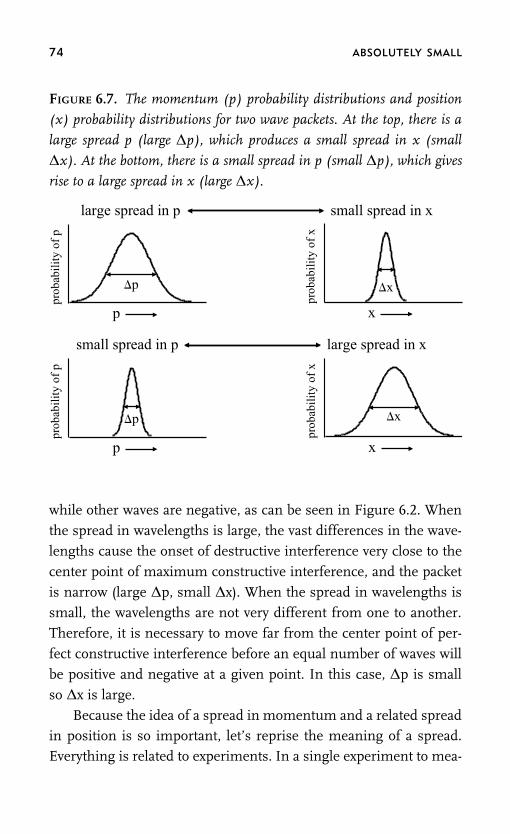
74 ABSOLUTELY SMALL
FIGURE 6.7. The momentum (p) probability distributions and position
(x) probability distributions for two wave packets. At the top, there is a
large spread p (large Δp), which produces a small spread in x (small
Δx). At the bottom, there is a small spread in p (small Δp), which gives
rise to a large spread in x (large Δx).
xpr
obab
ility
of
x
�x
p
prob
abili
ty o
f p
�p
large spread in p small spread in x
x
prob
abili
ty o
f x
�x
p
prob
abili
ty o
f p
�p
small spread in p large spread in x
while other waves are negative, as can be seen in Figure 6.2. When
the spread in wavelengths is large, the vast differences in the wave-
lengths cause the onset of destructive interference very close to the
center point of maximum constructive interference, and the packet
is narrow (large Δp, small Δx). When the spread in wavelengths issmall, the wavelengths are not very different from one to another.
Therefore, it is necessary to move far from the center point of per-
fect constructive interference before an equal number of waves will
be positive and negative at a given point. In this case, Δp is small
so Δx is large.
Because the idea of a spread in momentum and a related spreadin position is so important, let’s reprise the meaning of a spread.Everything is related to experiments. In a single experiment to mea-

HOW BIG IS A PHOTON 75
sure the momentum of a particle, only one value can be measured.
You have some instrument. It reads out a number. It can’t tell you
that the momentum is both 10 and 50 at the same time. In a single
measurement, a single well-defined value will be measured. How
do we get a single value when our wave packet has a spread in
momenta? The wave packet is made up of a superposition of mo-
mentum eigenstates, that is, momentum probability amplitudewaves with associated well-defined values of the momentum. When
a measurement is made, the nonnegligible disturbance accompany-
ing the measurement causes the system to ‘‘jump’’ from being in a
superposition state to a particular eigenstate. The measurement
gives the value of the momentum that goes with that eigenstate.
Now, the measurement changed the system. To make another mea-
surement, we need to start over and prepare the particle in the sameway. By preparing it in the same way, a wave packet composed of
the same superposition of momentum eigenstates will be gener-
ated. We now make the same measurement we did the first time.
In general, we will measure a different value of the momentum
because the wave packet is composed of many momentum waves
each with a different observable value of the momentum associated
with it. If we do this over and over again, each time preparing thewave packet in the same way and then making the measurement,
we will get a spread in the measured values of the momentum.
After a huge number of measurements, we might measure (neglect-
ing units) the value 400 a thousand times, 390 eight hundred times,
410 eight hundred times, but 200 and 600 only twenty times. If we
make a plot of all of these numbers we get a probability distribution
like those shown for momentum on the left side of Figure 6.7. Aprobability distribution is an experimental determination of the
composition of the wave packet. We now know how much (what is
the probability) of each wave in the packet. The same description
also applies to the position of our wave packet. On each measure-
ment of the position of identically prepared wave packets, a single

76 ABSOLUTELY SMALL
location for the particle will be found. After many measurements, a
distribution of positions is determined like those illustrated on the
right side of Figure 6.7.
THE HEISENBERG UNCERTAINTY PRINCIPLE
A very important point is that there is a relationship between thespread in momentum and the spread in position that is fundamen-
tal to the superposition state description of particles. When the
spread in momentum (Δp) is large, there are many waves spread
out along the x axis (see Figure 6.1) that combine to make the wave
packet. These waves have different wavelengths (see Figure 6.2).
When many waves with a wide range of wavelengths interfere, the
region of constructive interference dies out very fast away from themaximum (see Figures 6.3 and 6.4). That means that the spread in
position (Δx) is small. If there is only a small range of the momen-
tum waves that make up the wave pack (Δp small), then the spatial
region of constructive interference dies out slowly away from the
maximum in the position distribution (see Figure 6.7). Therefore,
the spread or uncertainty in position Δx is large. All of this occurs
because of the probability amplitude wave nature of the wave func-tions that describe the momentum eigenstates. A wave packet is
located, more or less, in the region of constructive interference, and
there is little probability of finding the particle in the regions of
substantial destructive interference.
The formal relationship between the spread in the momentum
and the spread in the position, that is, between Δp and Δx, is called
the Heisenberg Uncertainty Principle. Werner Karl Heisenberg(1901–1976) won the Nobel Prize in Physics in 1932 ‘‘for the cre-
ation of quantum mechanics, the application of which has, inter
alia, led to the discovery of the allotropic forms of hydrogen.’’ The
Heisenberg Uncertainty Principle is stated through a simple mathe-
matical relationship, ΔxΔp � h/4π, where h is Planck’s constant

HOW BIG IS A PHOTON 77
and the Δx and Δp define the widths of the distributions for posi-
tion and momentum, as shown in Figure 6.7. (� means greater
than or equal to.) Whether the equal sign (�) or the greater than
sign (�) applies depends on the shapes of the probability distribu-
tions. The equal sign applies for a shape called a Gaussian after
the great mathematician, Karl Friedrich Gauss (1777–1855). The
curves shown in Figures 6.5 through 6.7 are Gaussians. A Gaussianis the standard ‘‘bell-shaped curve’’ that describes the distributions
of things, such as test scores, for a properly designed test with a
large enough number of people taking the test. Gaussian-shaped
curves show up in many places in the physical sciences. The greater
than sign applies to other shapes. For any shape, which is made up
from a specific distribution of waves, it is possible to determine
what the product ΔxΔp will be, but it will always be �h/4π unlessthe shape is a Gaussian.
To understand the nature of the Uncertainty Principle, it is suf-
ficient to consider Gaussian shapes like those in Figure 6.7. Then,
ΔxΔp � h/4π. The equation shows what it is possible to know
simultaneously about the position and momentum of a particle.
h/4π is a constant. Therefore, ΔxΔp equals a constant. So if the
uncertainty in the momentum, Δp, is large, then the uncertainty inthe position, Δx, must be small, so that the product is h/4π. On the
other hand, if Δp is small, then Δx is large. The connection between
Δp and Δx is illustrated in Figure 6.7. The uncertainty principle
says that you can know something about the momentum of a parti-
cle and something about the position of a particle, but you can’t
know both the position and the momentum exactly at the same
time. This uncertainty in the simultaneous knowledge of the posi-tion and the momentum is in sharp contrast to classical mechanics.
It is fundamental to classical mechanics theory, as illustrated in
Figure 2.5, that the position and the momentum of a particle can
be precisely known (measured) simultaneously. Quantum theory
states that it is impossible to know both the position and the mo-

78 ABSOLUTELY SMALL
mentum precisely at the same time. We can know both within some
uncertainties, Δx and Δp.
Examining the Uncertainty Principle relationship, ΔxΔp � h/4π,
consider what happens as we make Δp smaller and smaller. As Δp
becomes smaller and smaller, Δx grows. Dividing both sides of the
equation by Δp gives Δx �h
4��p. As Δp becomes smaller, we are
dividing by a smaller and smaller number, so Δx grows. As Δp gets
closer and closer to zero, Δx gets closer and closer to infinity. In the
limit that Δp goes to zero, Δx goes to infinity. This limit has an
important meaning. If Δp is zero, the momentum is known pre-
cisely, but the position is totally unknown. With Δx � �, the parti-
cle can be found anywhere with equal probability. This result is in
accord with the discussion surrounding Figure 6.1, which shows
the wavefunction for a momentum eigenstate. When a particle is in
a momentum eigenstate, it has a perfectly well-defined value of its
momentum. However, its probability amplitude function, which de-
scribes the probability of finding the particle in some region of
space, is spread out (delocalized) over all space. The probability of
finding the particle anywhere is uniform; Δx � �. This is in con-
trast to the wave packets shown in Figure 6.7, where a superposition
of momentum eigenstates produces a state in which there is no
longer a perfectly well-defined momentum, but there is some
knowledge of the position. We know the position and momentum
within some ranges of uncertainty.
If we rearrange the uncertainty relation to give Δp �h
4��x, we
see that in the limit that Δx goes to zero (perfect knowledge of the
position), Δp goes to infinity. If we know the position perfectly, the
momentum can have any value. A wave packet composed of all of
the momentum eigenstates (Δp � �) has a perfectly well-defined
value of the position. It is possible to know p precisely but with no
knowledge of x; it is possible to know x precisely, but with no knowl-

HOW BIG IS A PHOTON 79
edge of p. This is called complementarity. You can know x or p but
not both at the same time. In classical mechanics, you can know x
and p. In quantum mechanics, you can know x or p. Generally for
quantum particles, absolutely small particles, you know something
about p and something about x, but you can’t know both precisely
simultaneously.

7
Photons, Electrons,
and Baseballs
PHOTONS, ELECTRONS, AND BASEBALLS are all described with quantum
theory in the same way, but quantum theory isn’t necessary to de-
scribe baseballs. Baseballs act as classical particles and behave in a
manner that is accurately described by classical mechanics. If pho-
tons, electrons, and baseballs all have the same quantum mechani-
cal description, why do only baseballs act as classical particles? Theanswer is that baseballs are large in the absolute sense. Here, we
will see why photons and electrons need a quantum theory descrip-
tion but baseballs do not. Real physical situations are discussed that
bring out both the wavelike and particlelike nature of quantum par-
ticles, that is, absolutely small particles.
WAVES OR PARTICLES?
When a particle is in a superposition state, a wave packet, we have
some knowledge of its position and some knowledge of its momen-
tum. So are photons, electrons, and so on waves or particles? The
answer is that they are wave packets. Whether they seem to be parti-
80
PHOTONS, ELECTRONS, AND BASEBALLS 81
cles or seem to be waves depends on what experiment you do, that
is, what question you ask. In the photoelectric effect, the photons
act like particles. One photon hits one electron, and kicks it out of
the metal (Figure 4.3). The photon is a wave packet formed from a
spread of momentum eigenstates. The width of the spread, Δp, re-
sults in a relatively well-defined position, that is, a relatively small
Δx. Thus, the photon wave packet is more or less well defined inposition, so that it can act like a particle of light in the photoelectric
effect. In the interference experiment (Figure 5.1), the photons act
like waves. This may not be surprising because the wave packet is,
in fact, a superposition of waves, but not waves in the normal classi-
cal sense, but rather probability amplitude waves. In the discussion
of the interference phenomenon, the photon wave is discussed as if
it is a single probability amplitude wave. Now it is clear that it isactually a wave packet, composed of a superposition of waves. When
it hits the beam splitter, it becomes a superposition of the two trans-
lation states, T1 and T2. The probability amplitude waves in T1 in-
terfere with their corresponding waves in T2, to produce the
interference pattern as discussed above.
DIFFRACTION OF LIGHT
So a photon acts like a particle in the photoelectric effect, but it can
also act like a wave. An experiment that clearly shows the wavelike
properties of photons is diffraction of light from a diffraction grat-
ing. It is possible to see diffraction using a music compact disk (CD)
and a bright light or sunlight. The CD has very fine grooves on its
surface. These are the tracks on which the information is stored. Asexplained below, when white light from the sun or a light bulb falls
on the CD, the grooves diffract the light, sending different colors in
particular directions. Different parts of the CD make a range of
angles relative to your eye, which causes the appearance of different
colors emanating from different parts of the CD.

82 ABSOLUTELY SMALL
Diffraction from a grating is used in many optical instruments,called spectrometers. These instruments separate the different col-ors of incoming light so that the colors can be analyzed individually.A recording of the colors of light from a particular source is calleda spectrum. For example, stars emit different colors of light depend-ing on their temperature. Taking a spectrum of the light from a starcan provide a great deal of information about the star. Star lighttraveling through space will encounter molecules in space. As dis-cussed in Chapter 8 and subsequent chapters, different moleculesabsorb different colors of light. Star light traveling to Earth hassome of its colors partially absorbed by the molecules in space. As-tronomers mount spectrometers on telescopes and take spectra todetermine what types of molecules are in space between a particularstar and the Earth.
Figure 7.1 shows the geometry for light diffraction from a grat-ing. The incoming light is at an angle α (Greek letter alpha) relative
FIGURE 7.1. Geometry of light diffraction from a grating. The grating is
composed of a reflective surface, usually silver or gold, with very fine
parallel grooves in it. The grating is shown here from the side. The grooves
run into the page. The grooves have a very uniform spacing, d; � is the
angle of the incoming light. The outgoing angles � depend on the color.
Therefore, the colors are separated by diffraction.
diffractiongrating
outgoing lightseparatedinto colors
normal
d
incominglight
diffractiongrating
normal
d
� �
incominglightincominglight
bluegreen
red
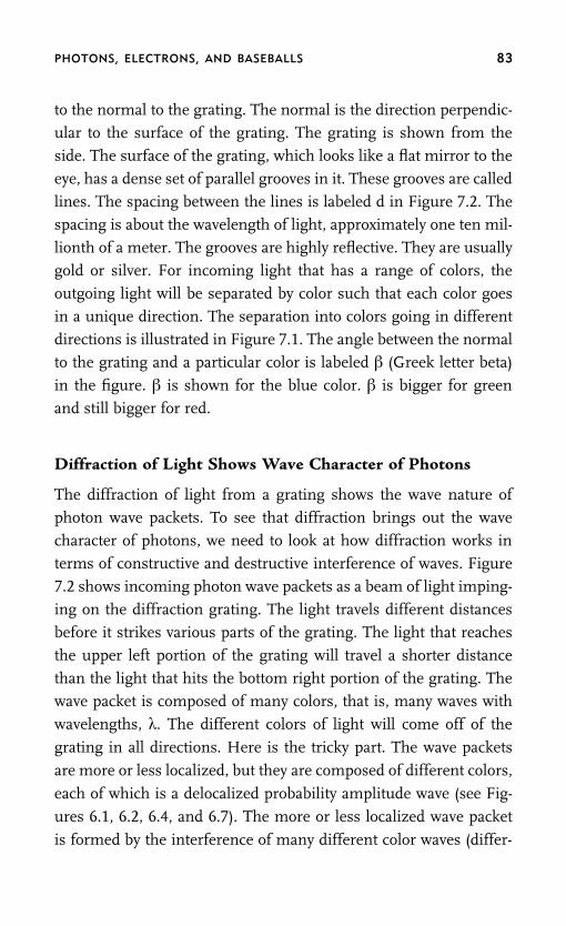
PHOTONS, ELECTRONS, AND BASEBALLS 83
to the normal to the grating. The normal is the direction perpendic-
ular to the surface of the grating. The grating is shown from the
side. The surface of the grating, which looks like a flat mirror to the
eye, has a dense set of parallel grooves in it. These grooves are called
lines. The spacing between the lines is labeled d in Figure 7.2. The
spacing is about the wavelength of light, approximately one ten mil-
lionth of a meter. The grooves are highly reflective. They are usually
gold or silver. For incoming light that has a range of colors, the
outgoing light will be separated by color such that each color goes
in a unique direction. The separation into colors going in different
directions is illustrated in Figure 7.1. The angle between the normal
to the grating and a particular color is labeled � (Greek letter beta)
in the figure. � is shown for the blue color. � is bigger for green
and still bigger for red.
Diffraction of Light Shows Wave Character of Photons
The diffraction of light from a grating shows the wave nature of
photon wave packets. To see that diffraction brings out the wave
character of photons, we need to look at how diffraction works in
terms of constructive and destructive interference of waves. Figure
7.2 shows incoming photon wave packets as a beam of light imping-
ing on the diffraction grating. The light travels different distances
before it strikes various parts of the grating. The light that reaches
the upper left portion of the grating will travel a shorter distance
than the light that hits the bottom right portion of the grating. The
wave packet is composed of many colors, that is, many waves with
wavelengths, λ. The different colors of light will come off of the
grating in all directions. Here is the tricky part. The wave packets
are more or less localized, but they are composed of different colors,
each of which is a delocalized probability amplitude wave (see Fig-
ures 6.1, 6.2, 6.4, and 6.7). The more or less localized wave packet
is formed by the interference of many different color waves (differ-

84 ABSOLUTELY SMALL
ent λs, which correspond to different momenta, p). Consider one
particular color, red, that comprises part of the wave packet. If the
wave hits only one line in the grating, it would reflect off in many
directions because of the shape of the groove. It would leave the
single groove as a superposition state composed of probability am-
plitude waves propagating in many directions. In the interferometer
(Figure 5.1), the incoming wave packet became a superpositionstate that had probability amplitude propagating in two directions.
Here, after hitting a single line, the superposition would be heading
in many directions.
The important feature of a grating is that the incoming wave
hits many lines in the grating. For a particular color, red shown in
Figure 7.2, there is a single direction in which the waves will add
up constructively. In the figure, for the direction in which the redwaves are propagating, all of the peaks and troughs of the waves
add in phase even though they reflect from different places. (The
wavelength has been exaggerated relative to the line spacing, d, to
make it easy to see the alignment of the waves.) The in phase addi-
tion of many waves leaving the grating makes a very large outgoing
wave. In all other directions, the red waves will add destructively
because the peaks and null do not line up.Diffraction from a grating causes the waves of a given wave-
length (a particular color) to add constructively in one direction.
The intensity associated with a probability amplitude light wave is
proportional the square of the wave amplitude. Therefore, in the
direction of constructive interference for a particular color, red in
the example, the intensity of light is large. In other directions, red
light will experience destructive interference, because the wave-length is such that the differences in the distances from each groove
don’t equal an integral number of wavelengths. For another color,
say blue, there is a different direction in which light coming off of
all of the grooves will add constructively (see Figure 7.1). Therefore,
the blue light component of the incoming photon wave packets will

PHOTONS, ELECTRONS, AND BASEBALLS 85
FIGURE 7.2. Incoming photon wave packets are diffracted from a grat-
ing. The different colors reflect off of the grooves. For a particular color,
there is a direction in which the waves corresponding to that color con-
structively interfere. They add to make a large amplitude wave, so the
color looks very bright in that particular direction.
outgoingwaves
Peaks line upConstructive interference
light
Look in one direction,see one color
incoming
leave the grating as a large amplitude wave in its own direction, and
in this direction the intensity of the blue component of the incom-ing light will appear bright.
Electrons Act Like Bullets in a Cathode Ray Tube
Diffraction of light from a grating brings out the wave property of
the photon wave packets, while the photoelectric effect demon-strates the more localized particle like properties of a photon wave
packet. In the discussion of the de Broglie wavelength, which relates
the momentum to a wavelength through the relation p � h/λ, it
was mentioned that the descriptions of electrons and other types of
‘‘particles’’ are the same as the description of photons. Both photons

86 ABSOLUTELY SMALL
and electrons are described in terms of probability amplitude waves.
Both are more or less localized wave packets (see Figure 6.7). For
an electron that is a free particle (no forces are acting on it) the wave
packet is a superposition of the free particle momentum eigen-
states. The uncertainty in the electron’s position, Δx, is determined
by the uncertainty (spread) in the momentum, Δp, through the
Heisenberg’s uncertainty relationship, ΔxΔp � h/4π. The equalitysign holds for Gaussian wave packets, which are the shapes shown
in Figure 6.7.
To illustrate both the particle nature and wave nature of elec-
trons, two examples are discussed: how a cathode ray tube (CRT)
works and low energy electron diffraction from a crystal surface.
Cathode ray tubes used to be ubiquitous. They are the devices that
produce the pictures in the original televisions and computer moni-tors. CRTs are the large, boxy TVs and monitors that are rapidly
being replaced by other devices, such as liquid crystal displays
(LCDs). (There are actually several technologies used to make large-
screen thin TVs, but thin computer monitors are all LCDs.)
Figure 7.3 is a schematic diagram of a CRT. Inside the CRT is
a vacuum in which electrons can move without colliding with air
molecules. The process that produces the picture begins with thefilament, a piece of wire (left side of figure). An electrical current is
passed through the filament, which causes it to get very hot like the
filament in a conventional light bulb, the element in an electric
stove, or the element in an electric space heater. The heat from the
filament heats the cathode until it is also very hot. The cathode is a
piece of metal that is connected to a negative voltage, like the nega-
tive end of a battery, but at a much higher voltage. The cathodebecomes so hot that electrons boil off. Heat is a form of energy. The
electrons are held in the metal by a binding energy that depends on
the type of metal. When the metal is hot enough, the thermal en-
ergy can overcome the electron binding energy and some electrons
will leave the metal. In the photoelectric effect, a photon provided

PHOTONS, ELECTRONS, AND BASEBALLS 87
FIGURE 7.3. A schematic of a cathode ray tube (CRT). The hot filament
heats the cathode, which ‘‘boils’’ off electrons. The positively charged ac-
celeration grid accelerates the negatively charged electrons. Voltages ap-
plied to the control grids steer the electrons to particular points on the
screen. The screen is covered with tiny adjacent red, green, and blue spots
that glow with their particular color when hit with electrons. By rapidly
scanning the electron beam to hit the appropriate colors in a given spot
on the screen the image is made.
cathode
filament
controlgrid
screenelectronsboil off
electrons aimedelectronshit screen
accelerationgrid
+
e-
+
the energy to overcome the electron binding to the metal. In a CRT,heat provides the energy to eject the electrons from the metal. Theelectrons that leave are replaced by the connection to the negativepower supply that puts electrons back into the cathode, so the proc-ess can go on continuously. Electrons are negatively charged, andbecause the cathode is at a negative voltage, the electrons are re-pelled from the cathode. Therefore, the electrons fly away from thecathode. The movement of the electrons away from the cathode ishelped by the positively charged acceleration grid (see Figure 7.3).Because the acceleration grid is connected to a positive power sup-ply, the negatively charged electrons are attracted to it. Like chargesrepel. Unlike charges attract. The acceleration grid is a mesh ofwires that is mostly holes. When the electrons reach the grid, mostof them fly right through it and keep going, moving very fast.

88 ABSOLUTELY SMALL
The electrons then pass between the control grids (see Figure
7.3), which control the direction the electrons go. There is one pair
of control grids for the vertical direction (shown in the figure) and
an equivalent set for the horizontal direction (not shown). Consider
the vertical direction. If a positive voltage is applied to the top con-
trol grid and a negative voltage is applied to the bottom control grid,
the electrons will be deflected up, as shown in Figure 7.3, becausethe negatively charged electrons will be attracted toward the positive
top grid and repelled from the negative bottom grid. If the polarity
of the voltages on the two grids is reversed, the electrons will be
deflected downward. If large voltages are applied to the grids, the
electrons will be deflected a lot. If small voltages are applied, the
electrons will be deflected a small amount. If no voltages are ap-
plied, the electrons will go straight ahead. The same thing happensby applying voltages to the horizontal control grids. Once the elec-
trons pass by the control grids, they continue in a straight line. In
this manner, the electrons can be aimed just like bullets. This part
of the CRT is referred to as an electron gun. Electron guns are used
in many scientific devices such as electron microscopes and the
device discussed below. So even when there are no more CRTs used
as TVs and computer monitors, the basic device described here willstill be important.
Because there is no air and gravity is a very weak force, the
electrons travel basically as free particles until they hit the screen
shown on the right side of Figure 7.3. On the screen are very small
and very closely spaced patches of chromophores. Chromophores
are chemical species that emit light when excited, that is, when
sufficient energy is imparted to them. In this case, the chromo-phores are excited when the electrons hit them. In each very small
region of the screen, there are three chromophores, one red, one
green, and one blue. The electron beam can be aimed to hit a partic-
ular spot with great accuracy. If at a given location the red chromo-
phore is hit, the screen lights up for an instant with a tiny red dot
PHOTONS, ELECTRONS, AND BASEBALLS 89
of light. If the green chromophore is hit, there is a green dot of light,
and if the blue chromophore is hit, a blue dot of light is generated,
The electronics that produce the voltages on the control grids
sweep the electron beam across the screen horizontally, then move
the beam down, and sweep horizontally again. This is continued
until the entire screen is swept. The beam returns to the top, and
the sweep is repeated. As the beam sweeps, it is directed to hit red,green, or blue chromophores. The patches of three chromophores
are so close together horizontally and vertically that your eye cannot
distinguish them as individual dots. The beam can also be turned
off so if no chromophore is hit you get a black spot. The combina-
tion of the three colors is sufficient to make any color. The image
that we see on a CRT computer screen or a TV is formed by control-
ling which colors are hit and which spots are not hit at all. Theelectron beam is moved across the screen so fast that our eyes can-
not tell that what we see is actually a very rapid succession of still
pictures.
In the description of the CRT, the electrons acted very much
like our general conception of particles. They could be aimed by the
electron gun to hit very specific spots on the screen. This does not
sound very much like a wave. However, it is certainly within ourdescription of more or less localized wave packets. As long as Δx
of the electron wave packets is small compared to the size of the
chromophore spots (pixels), the fact that the wave packet is delocal-
ized over a distance scale Δx doesn’t matter. The colored pixels are
small, but not small on the ‘‘absolutely small’’ distance scale. They
are smaller than the eye can see without a microscope, but that is
still large compared to the length scales that are encountered inatomic and molecular systems. Therefore, wave packets with a rea-
sonably small Δp can still have an uncertainty in position that is
very small compared to the pixel size. For a particle, such as an
electron, p � mV, where m is the mass of the electron and V is the
velocity of the electron. The mass is well defined. The uncertainty

90 ABSOLUTELY SMALL
in p comes from an uncertainty in the velocity. So what Δp means
is that the velocity is not perfectly well defined. Measurements of
the velocity on identically prepared electron wave packets will not
give the same value from one measurement to the next. The uncer-
tainty in the velocity yields an uncertainty in the momentum, Δp,
which through the Uncertainty Principle, ΔxΔp � h/4π, gives the
uncertainty in x, Δx. The important point is that Δx can be signifi-
cant on the distance scale of atoms and molecules but very small
compared to the distance scale of the macroscopic colored pixels on
the CRT screen. In such situations, the wave nature of a wave packet
is not manifested, and the wave packet behaves like a classical par-
ticle.
Electrons Act Like Waves in Electron Diffraction
Electron wave packets also display their wave properties, as illus-
trated in Figure 7.4. In this experiment, a beam of electrons gener-
ated with an electron gun, like that described above, is aimed at a
crystal surface rather than a TV screen. The electrons are not of
sufficiently high energy to penetrate the crystal. The surface of the
crystal is composed of rows of atoms called a lattice or crystal lattice.
The rows of atoms are spaced a few angstroms apart; one angstrom
is 1 � 10�10 m, or one ten billionth of a meter. On the atomic
distance scale, the unit of angstroms comes up often. It is given a
special symbol, A. The spacing is determined by the size of the
atoms. The rows of atoms act as the grooves in a diffraction grating,
but they are much more closely spaced. The wavelength of the elec-
trons is on the same distance scale as the lattice spacing (row spac-
ing). The wavelength is given by the de Broglie relation λ � h/p. p
� mV. The mass of the electron is 9.1 � 10�31 kg (kilograms).
Then for a velocity of 7.3 � 105 m/s (730,000 meters per second,
about 1.6 million miles per hour), λ � 10 A. This velocity is very
easily obtained with a simple electron gun.

PHOTONS, ELECTRONS, AND BASEBALLS 91
FIGURE 7.4. A schematic of low-energy electron diffraction (LEED) from
the surface of a crystal. An incoming beam of electrons, with low enough
energy not to penetrate the crystal, strikes the surface. The lines of atoms
act like the grooves of the diffraction grating in Figure 7.1. They diffract
the incoming electron waves.
Peaks line up Constructive interference
outgoingwaves
incomingelectronwave packets
crystalsurface
The electron probability amplitude waves diffract from the crys-tal surface in a manner akin to the photons diffracting from theruled grating discussed above. However, in the ruled grating, thereis a single separation, d, because the grooves all run parallel to eachother in a single direction. The lattice at a crystal surface is two-dimensional. As can be seen in Figure 7.5, there are many direc-tions in which there are parallel rows of atoms. The solid lines showrows of atoms running in different directions. The dashed line par-allel to each solid line shows that there are parallel rows of atomsfor each of the directions indicated by the solid lines. For the rowsof atoms running in different directions, the spacing between theatoms (the diffraction groove spacing) is different. The differencein spacing can be seen in Figure 7.5. Look at the separation betweena pair of solid and dashed lines. Each pair has a different separation,which is the groove spacing.

92 ABSOLUTELY SMALL
FIGURE 7.5. The lattice from Figure 7.4, with examples of different rows
of atoms shown by the lines. For each line passing through the centers of
atoms in a row, it is possible to draw more lines that are parallel to the
initial line and that also pass through the centers of atoms. The spacings
between these distinct parallel rows are different. Each set of rows causes
diffraction in a different direction.
Because there are many different atom-to-atom spacings with
the ‘‘grooves’’ running in different directions, the electrons’ waves
will be diffracted in many different directions. Figure 7.6 is an ex-
ample of low-energy electron diffraction from a crystal surface. The
black circle in the center is a piece of metal called a beam stop. It is
supported by another piece of metal that appears as the vertical bar
below the beam stop in the picture. The beam stop prevents the
portion of the electron beam that is reflected from the crystal from
hitting the detector. The brighter and dimmer white spots are pro-
duced by the diffracted electrons hitting the detector. From the loca-
tion of the spots, the spacing and arrangement of the atoms can be
determined. Electron diffraction from crystal surfaces is an impor-
tant tool in the science of understanding the nature of surfaces. The
electron diffraction pattern demonstrates conclusively that electrons
can behave as waves, just like photons.

PHOTONS, ELECTRONS, AND BASEBALLS 93
FIGURE 7.6. Experimental data showing diffraction of electrons from the
surface of a crystal. The various light spots are the electron diffraction
spots. There are many spots because the diffraction occurs from the many
different parallel rows of atoms (see Figure 7.5).
ELECTRONS AND PHOTONS ARE PARTICLESAND WAVES, BUT BASEBALLS ONLY PARTICLES
Electrons act as particles in a CRT just as photons act as particles inthe photoelectric effect. Electrons act as waves in low-energy elec-tron diffraction just as photons act as waves when they diffract froma diffraction grating. In reality, photons, electrons, and all particlesare actually wave packets that are more or less localized. Wave pack-ets can display their wavelike properties or their particlelike proper-ties depending on the circumstances.
If photons and electrons can show both wavelike and particle-like properties, why don’t baseballs? To see the reason that baseballsact like particles in the classical mechanics sense, we need to lookat the wavelengths associated with particles versus their size.
First consider an electron in an atom such as hydrogen. We aregoing to talk about the quantum description of the hydrogen atomand other atoms in Chapters 10 and 11, but for now, we will onlyuse a very simple qualitative discussion of the wavelike characteris-tics of the hydrogen atom. The de Broglie relation tells us that the

94 ABSOLUTELY SMALL
wavelength λ � h/p. The momentum is p � mV, the mass times
the velocity. The mass of an electron is me � 9.1�10�31 kg. In an
atom, the typical velocity of an electron is V � 5.0�106 m/s. Then
the de Broglie wavelength is
� �hp�
6.6�10�34 J-s(9.1�10�31 kg)(5.0�106 m/s)
�1.5�10�10 m�1.5A.
Note that 1.5 A is approximately the size of an atom. Therefore, the
wavelength of an electron in an atom is about the size of the atom.
The wave properties of electrons will be very important when elec-
trons are in systems that are very small like atoms.
What about a baseball? According to the rules of Major League
Baseball, a baseball must weigh between 142 g and 149 g. We will
take the mass to be 145 g � 0.145 kg. A pretty fast pitch goes 90
mph. 90 mph � 40 m/s. The momentum of a fast ball is p � 0.145
kg � 40 m/s � 5.8 kg-m/s. The de Broglie wavelength of the fast
ball is:
� �hp�
6.6�10�34 J-s(0.145 kg)(40 m/s)
�1.1�10�34 m � 1.1�10�24 A.
This is an unbelievably small number. The size of one atom is about
1 A. The size of the nucleus of an atom is about 10�5 A. Then the
wavelength of a baseball is 0.0000000000000000001 of the size of
one atomic nucleus. This wavelength is small beyond small. It is so
small that it will never be manifested in any measurement. There
can never be a diffraction grating with line spacing small enough to
show diffraction for a wavelength that is a ten millionth of a tril-
lionth of the size of an atomic nucleus. Because this wavelength is
so small we never have to worry that a baseball will diffract from a
baseball bat. It will always act like a classical particle. Objects that
are large in the absolute sense have the property that the wave-
lengths associated with them are completely negligible compared to
their size. Therefore, large particles only manifest their particle na-

PHOTONS, ELECTRONS, AND BASEBALLS 95
ture; they never manifest their wave nature. In contrast, particles
that are small in the absolute sense have de Broglie wavelengths
that are similar to their size. Such absolutely small particles will act
like waves or act like particles depending on the situation. They are
wave packets. In the manner that we have discussed, they are both
waves and particles.
8
Quantum Racquetball and
the Color of Fruit
IN THE PREVIOUS CHAPTERS, the fundamental concepts of quantum
theory were introduced and explained. The examples given, how-
ever, looked only at the behavior of free particles. It was shown that
electrons could behave as particles in the discussion of how a CRT
works, but they behaved as waves in the description of electron dif-
fraction from crystal surfaces. A free particle can have any energy.Its energy, which is kinetic, is determined by its mass and its veloc-
ity. As the velocity increases, the energy increases. A tiny increase
in velocity produces a tiny increase in energy. A large increase in
velocity produces a large increase in energy. The steps in energy
can be any size; they are continuous. Bound electrons were dis-
cussed briefly in connection with the photoelectric effect. It was
pointed out that if the energy of the incoming photon is insufficientto overcome the binding of electrons in the metal, no electrons will
be ejected from the metal. Electrons bound to nuclei of atoms are
responsible for the properties of atoms and molecules. It was also
mentioned that Planck explained black body radiation, which will
be discussed in detail later, by postulating that bound electron ener-
96

QUANTUM RACQUETBALL 97
gies can only change in discreet steps. To understand the properties
of the atomic and molecular matter that surrounds us in everyday
life, it is necessary to treat bound electrons with quantum theory.
The essential feature of electrons bound to an atom or molecule
is that their energy states are discreet. We say that the energies an
electron can have are quantized, that is, an electron bound to an
atom or molecule can only have certain energies. The energy goesin steps, and the steps are certain discreet sizes. The energy states
are like a staircase. You can stand on one stair, or you can stand on
the next higher stair. You cannot stand halfway between two stairs.
These discreet or quantized energies are frequently called energy
levels. Unlike a staircase, the energy levels are not generally equally
spaced.
An important area of modern quantum theory research is thecalculation of the electronic quantum states of molecules. This field
is called quantum chemistry. Such calculations yield the quantized
energies of electrons in molecules (energy levels), and they also cal-
culate the structures of molecules. Molecular structure calculations
give the distances between atoms and the positions of all atoms
in a molecule within limits set by the uncertainty principle. Thus,
quantum mechanical calculations are able to determine the size andshapes of molecules. Such calculations are important for under-
standing the basic principles of the bonding of atoms to form mole-
cules and to design new molecules. As quantum theory continues
to develop and the ability to solve complex math problems on in-
creasingly fast and sophisticated computers continues to advance,
larger and larger molecules can be investigated using quantum
chemistry. One area of great importance is the quantum theory de-sign of pharmaceuticals. Molecules can be designed to have the
right size and shape to ‘‘fit’’ into a particular location in a protein or
enzyme.
Quantum chemistry is mathematically very intense. Even the
quantum mechanical calculation of the simplest atom, the hydro-

98 ABSOLUTELY SMALL
gen atom, is mathematically complex. The hydrogen atom consists
of a single electron bound to a single proton. The proton, which is
the nucleus of a hydrogen atom, is positively charged and the elec-
tron is negatively charged. It is the attraction of the negative electron
to the positive proton that holds the hydrogen atom together. The
detailed calculation of the energy levels of the hydrogen atom will
not be presented, but in the next chapters, the results of the calcula-tions are discussed in some detail. The calculations give the hydro-
gen atom energy levels and the hydrogen atom wavefunctions. The
wavefunctions, that is, the probability amplitude waves for the hy-
drogen atom, are the starting point for understanding all atoms and
molecules. Atoms and molecules are complicated because they are
absolutely small three-dimensional systems, and it is necessary to
deal with how protons and electrons interact with each other.
THE PARTICLE IN A BOX—CLASSICAL
There is a very simple related problem called the particle in a box.
We can solve this problem without complicated math. The solutions
to the particle in a box problem make it possible to illustrate many
of the important properties of bound electrons, such as quantizedenergy levels and the wavelike nature of electrons in bound states.
Before analyzing the nature of an electron in an atomic-sized one-
dimensional box, the classical problem of an ideal one-dimensional
racquetball court will be discussed so that the differences between a
classical (big) system and a quantum mechanical (absolutely small)
system can be brought out.
Figure 8.1 is an illustration of a perfect ‘‘box.’’ It is one dimen-sional. The walls are taken to be infinitely high, infinitely massive,
and completely impenetrable. There is no air resistance inside the
box. In the figure, the inside of the box is labeled as Q � 0, and
outside of the box, Q � �. Earlier we said that a free particle is a
particle with no forces acting on it. For a force to be exerted on a

QUANTUM RACQUETBALL 99
FIGURE 8.1. A perfect one-dimensional box. The walls are infinitely
high, infinitely thick, infinitely massive, and completely impenetrable.
There is no air resistance in the box. In the box, Q, the potential energy
is zero, and outside the box, it is infinite. The box has length, L.
Q =Q = 0
L
� �
0
Q =
x
particle, there must be something for the particle to interact with.For example, a negatively charged particle like an electron can inter-act with a positively charged proton. The attractive interaction be-tween the oppositely charged particles will exert a force on theelectron. In the description of electron steering in a CRT (see Figure7.3), an electric field exerted a force on the electrons, causing themto change direction. A measure of the interaction of a particle withsome influence on it, such as an electric field, is called a potentialand has units of energy. In the figure, the potential is labeled Q.Inside the box, Q � 0, just as in a free particle. This means theparticle is not interacting with anything inside the box. There areno electric fields or air resistance. However, outside the box, Q �
�. An infinite potential for the particle means the particle wouldhave to have infinite energy to be located in the regions outside thebox. Q � � is just the formal way of stating that the walls areperfect. There is no possibility of the particle penetrating the wallsor going over the top of the walls no matter how much energy ithas. Therefore, if a particle is put inside the box, it is going to stay

100 ABSOLUTELY SMALL
inside the box. There is no way for it to escape. In this sense, the
particle is bound inside the box. It can be in the space of length L,
but nowhere else.
Figure 8.2 shows a racquetball bouncing off of the walls in a
perfect one-dimensional classical (big) racquetball court. As dis-
cussed, the walls are perfect, and there is no air resistance. In addi-
tion, the ball is perfect, that is, it is perfectly elastic. When a ball
hits a wall, it compresses like a spring and springs back, which
causes the ball to bounce off the wall. A real ball is not perfectly
elastic. When the ball compresses, not all of the energy that went
into compressing the ball goes back into pushing the ball off of the
wall. Some of the energy that went into compressing the ball goes
into heating the ball. However, here we will take the ball to be per-
fectly elastic. All of the kinetic energy of the ball that compresses it
when it hits the wall goes into pushing the ball off of the wall.
FIGURE 8.2. A ball in a perfect one-dimensional racquetball court. There
is no air resistance, and the ball is perfect. When the ball strikes the wall
at L, it bounces off, hits the wall at 0, and keeps bouncing back and forth.
Because the court is perfect, the ball is perfect, and there is no air resis-
tance; once the ball starts bouncing, it keeps bouncing back and forth
indefinitely.
L0 x

QUANTUM RACQUETBALL 101
Therefore, the speed of the ball just before it hits the wall is equal
to the speed of the ball after it bounces off.
In this perfect racquetball court, the ball bounces off of the walls
without losing any energy and there is no air resistance or gravity.
Therefore, the ball will bounce back and forth between the walls
indefinitely. It will hit the wall at position L, bounce off, and then
hit the wall at position 0, bounce off, and just continue bouncingback and forth. Because the potential inside the box is zero (see
Figure 8.1), there are no forces acting on the ball. Therefore, its
energy is purely kinetic energy, Ek �12mV2; m is the mass of the
ball and V is its velocity. If the ball is hit a little bit harder, it will go
a little bit faster, that is, V will be a little bit bigger. Ek will be a little
bigger. If the ball is hit somewhat more gently, the ball’s velocity
will be a bit smaller, and Ek will be a little smaller. In this perfectracquetball game, the energy can vary continuously. Ek can go up or
down by any amount, the amount depending only on how hard you
hit the ball.
Another important feature of classical racquetball is that it is pos-
sible to stop the ball and put it on the floor. In this situation, the ball
has no velocity, V � 0. If V � 0, then Ek � 0. If V � 0, then the
momentum is zero because p � mV. So we know the momentum
exactly. If the ball is placed on the floor with V � 0, then the position
is known. If the position is called x (see Figure 8.2), x can take on
values between 0 and L. It cannot have any other values because the
ball is inside the court (the box) and can’t get out because of the
perfect walls. The ball can be placed at a certain position x on the
floor of the court. Therefore, its position is known exactly. This is a
characteristic of a macroscopic racquetball court, even a perfect one.
It is a classical system, and it is possible to know simultaneously
both the momentum, p, and the position, x, precisely.
A racquetball court is 40 feet long (about 12 m), and a ball is
2.25 inches in diameter and weighs 1.4 ounces (about 0.04 kg).

102 ABSOLUTELY SMALL
Clearly, racquetball is a game describable by classical mechanics.You can watch the ball bounce back and forth by observing it withlight without changing it.
PARTICLE IN A BOX—QUANTUM
What are the differences if we now consider quantum racquetball?The court is still perfect, but now its length is 1 nm (10�9 m) ratherthan 12 m. Furthermore, the particle now has the mass of an elec-tron, 9.1 � 10�31 kg rather than 0.04 kg. This is the quantum parti-cle in a box problem.
We can immediately say that the lowest energy of a quantumparticle in a 1-nm-length box cannot be zero. In the classical rac-quetball court, the velocity V could be zero, which means the mo-mentum, p � mV is zero. In addition, the position x could have aperfectly well-defined value. For example, the ball could be standingstill (V � 0) exactly in the middle of the court, which would be x �
L/2. Then, for our classical racquet ball, Δp � 0 and Δx � 0. Theproduct, ΔxΔp � 0, is not in accord with the Heisenberg Uncer-tainty Principle, which is okay because this is a classical system.However, the absolutely small particle in the nanometer size box isa quantum particle, and it must obey the Uncertainty Principle, thatis, ΔxΔp � h/4π. If V � 0 and x � L/2, we know both x and p. Theresult would be ΔxΔp � 0, the same as the classical racquetball.This is impossible for a quantum system. Therefore, V cannot bezero. The particle cannot be standing still at a specific point. If Vcannot be zero, then Ek can never be zero. The Uncertainty Princi-ple tells us that the lowest energy that a quantum racquetball canhave cannot be zero. Our quantum racquetball can never stand still.
ENERGIES OF A QUANTUMPARTICLE IN A BOX
What energies can a quantum particle in a nanometer-size boxhave? This question can be answered without a great deal of math,

QUANTUM RACQUETBALL 103
but we need to think about waves again. In Chapter 6, we discussed
the wavefunctions for free particles. The wavefunction for a free
particle with a definite momentum p is a wave that extends through-
out all space. So an electron with a perfectly well-defined momen-
tum is a delocalized wave over all space. The probability of finding
a free electron is equal everywhere. Such an electron has a well-
defined kinetic energy, Ek � 1/2mV2, because it has a well-definedmomentum, p � mV.
An electron in a nanometer-size box is something like our free
particle in the sense that inside the box, Q � 0. Inside the box there
is no potential, which means that there are no forces acting on the
particle. This is just like the free particle; there are no forces acting
on a free particle. However, there is a major difference between a
particle in the box and a free particle, the walls of the box. An elec-tron in a box is located only inside the box. Its wavefunction cannot
be spread over all space because of the perfect nature of the box.
The particle is inside the box and can’t ever be outside the box. The
wavefunction gives the probability amplitude of finding the particle
in some region of space. This is the Born interpretation of the wave-
function. If our electron can only be found inside the box and never
outside of the box, there must be finite probability of finding theparticle inside the box but zero probability of finding the particle
outside the box. If the probability of finding the particle outside the
box is zero, then the wavefunction must be zero for all locations
outside the box.
The result of the reasoning just presented is that the wavefunc-
tion for a particle in a box is like a free particle wavefunction, but the
wavefunction must be zero outside the box. In his interpretation ofthe nature of the quantum mechanical wavefunction, Born placed
certain physical constraints on the form wavefunctions can have. One
of these is that a good wavefunction must be continuous. This condi-
tion means that the change in the wavefunction with position must
be smooth. An infinitesimal change in position cannot produce a
sudden jump in the probability. This is really a simple idea. If the
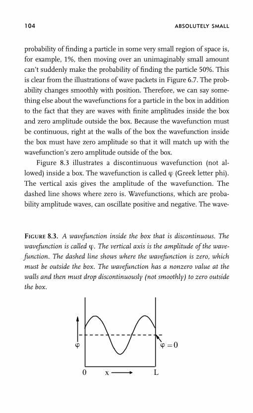
104 ABSOLUTELY SMALL
probability of finding a particle in some very small region of space is,
for example, 1%, then moving over an unimaginably small amount
can’t suddenly make the probability of finding the particle 50%. This
is clear from the illustrations of wave packets in Figure 6.7. The prob-
ability changes smoothly with position. Therefore, we can say some-
thing else about the wavefunctions for a particle in the box in addition
to the fact that they are waves with finite amplitudes inside the box
and zero amplitude outside the box. Because the wavefunction must
be continuous, right at the walls of the box the wavefunction inside
the box must have zero amplitude so that it will match up with the
wavefunction’s zero amplitude outside of the box.
Figure 8.3 illustrates a discontinuous wavefunction (not al-
lowed) inside a box. The wavefunction is called (Greek letter phi).
The vertical axis gives the amplitude of the wavefunction. The
dashed line shows where zero is. Wavefunctions, which are proba-
bility amplitude waves, can oscillate positive and negative. The wave-
FIGURE 8.3. A wavefunction inside the box that is discontinuous. The
wavefunction is called . The vertical axis is the amplitude of the wave-
function. The dashed line shows where the wavefunction is zero, which
must be outside the box. The wavefunction has a nonzero value at the
walls and then must drop discontinuously (not smoothly) to zero outside
the box.
x L0
� � = 0

QUANTUM RACQUETBALL 105
function shown in Figure 8.3 has values at the walls that are not 0.
However, the wavefunction must be zero outside the box, that is,
for values of x less than 0 and greater than L it must be zero. As
drawn, the wavefunction jumps suddenly from nonzero values at
the walls to zero values immediately beyond the walls outside the
box. Therefore, the wavefunction as drawn in Figure 8.3 is not a
good wavefunction because it is not continuous. This function can-
not represent a quantum particle in the box.
Wave Function Must Be Zero at the Walls
For the wavefunctions representing the particle in the box to be
physically acceptable functions, their values at the walls must be
zero so that there is no discontinuity at the walls. This is not a
difficult condition to meet. Figure 3.1 illustrates a wave in free
space. It oscillates positive and negative. Every time it goes from
positive to negative or negative to positive, it crosses through zero.
In fact, the zero points are separated by one-half of a wavelength.
So what we need to do to get good particle in a box wavefunctions
is pick waves with wavelengths such that they fit in the box with
their zero points right at the walls. Figure 8.4 shows three examples
of waves that are acceptable particle in the box wavefunctions. The
one on the bottom, labeled n � 1, is composed of a single half
wavelength. It starts on the left with an amplitude of 0, goes
through a maximum, and then is zero again at the wall at position
L. The next wave up, labeled n � 2, is one full wavelength. Again,
it starts at the left wall with amplitude zero, goes through a positive
peak, back through zero, a negative peak, and is zero at the wall at
position L. The wave labeled n � 3 is one and one-half wavelengths.
Any wave that is an integer number of half wavelengths, that is 1,
2, 3, 4, 5, etc. half wavelengths, and has a wavelength so that it starts
at zero on the right and ends at zero on the left is okay.
The label n is the number of half wavelengths in the particular

106 ABSOLUTELY SMALL
FIGURE 8.4. Three examples of wavefunctions, , inside the box that are
continuous. They have been shifted upward for clarity of presentation.
The vertical axis is the amplitude of the wavefunction. The dashed line
shows where the wave function is zero, which it must be outside the box.
The wavefunctions, which have zero values at the walls, are continuous
across the walls.
L0
� �
�
� = 0
= 0
= 0
n = 1
n = 2
n = 3
x
wavefunction. For n � 1, the wavelength, λ, is 2L because the box
has length L, and n � 1 corresponds to a half wavelength. For n �
2, the wavelength is L because exactly one wavelength fits between
the walls. For n � 3, 3 half wavelengths � L. That means 1.5λ �
L. Then λ � L/1.5, so λ � 2L/3. Notice that there is a general rule
here. λ � 2L/n, where n is an integer. For n � 1, λ � 2L. For n �
2, λ � 2L/2 � L. For n � 3, λ � 2L/3, and so forth.
Nodes Are Points Where the Wavefunction Crosses Zero
Nodes are another important feature of the wavefunctions. Nodes
are points where the wavefunction crosses zero, going from positive

QUANTUM RACQUETBALL 107
to negative, or negative to positive. The n � 1 wavefunction has no
nodes. The n � 2 wavefunction has one node right in the middle
of the box. The n � 3 wavefunction has two nodes. Nodes are points
(other than at the walls) where the probability of finding the particle
is zero. In a classical system, as in Figure 8.2, the ball bounces back
and forth. It can be at any location. But a particle in a quantum box
has certain places (nodes) where the probability of finding it is zero.
No matter how many measurements are made on identically pre-
pared systems, we will never find the particle at a node.
Figure 8.4 shows the probability amplitude waves. As discussed,
the probability of finding the particle in a certain region of space is
proportional to the square of the wavefunction (actually the absolute
value squared, but for our purposes, there is no difference). Figure
8.5 shows the square of the wavefunctions that are displayed in
Figure 8.4. The square of the wavefunctions are always positive be-
cause the probability of finding a particle in some region of space
cannot be negative. Where the amplitude is large, there is a large
probability of finding the particle. As n increases, the number of
nodes increases. As we will discuss in the next and later chapters,
atomic and molecular wavefunctions also have nodes.
A question that is frequently asked is, how does a particle get
through a node? For example, for n � 2, there is a node exactly in
the middle of the box. In a classical system if we had a ball on the
left side of the box and it was traveling to the right, but we said it
could never be in the center of the box, we would be confident that
the ball could never get to the right side of the box. However, we
cannot think classically about an absolutely small particle, such as
an electron in a molecular-sized box. It does not have a simultane-
ous definite position and momentum that can be described by an
observable trajectory. A quantum particle, an electron, is described
as a probability amplitude wave. Waves have nodes. Even classical
waves have nodes. A quantum particle does not have to ‘‘pass

108 ABSOLUTELY SMALL
FIGURE 8.5. The squares of the first three wavefunctions, 2, for the par-
ticle in a box. They have been shifted upward for clarity of presentation.
The vertical axis is the amplitude of the wavefunction squared. The
dashed line shows where the wavefunction is zero. The square of the
wavefunctions are always positive because they represent probabilities.
The wavefunctions shown in Figure 8.4 can be positive or negative.
n = 1
n = 2
n = 3
L0 x
= 0
= 0
= 0
2�
2�
2�
2�
through’’ a node because it is a delocalized probability amplitudewave. The idea of a trajectory in which to get from point A to point
B a particle must pass through all the points in between just doesn’t
apply to the proper wave description of electrons and other abso-
lutely small particles.

QUANTUM RACQUETBALL 109
The Energies Are Quantized
Now we will determine the possible energies that an absolutelysmall particle in a box can have. The classical ball in a racquetballcourt can have any energy, and the energy is continuous. We candetermine what energies a particle, such as an electron, can have ina tiny box by using the rule for the possible wavelengths, λ � 2L/n,that allowed probability amplitude waves can have inside the box(see Figure 8.4). Here tiny means a box that is small in the absolutesense, that is, the wavelength is comparable to the size of the box.We will also need several other physical relationships that we havemet previously. The other relations we need are the de Broglie wave-length, p � h/λ, where p is the momentum and h is Planck’s con-stant; the fact that the momentum is p � mV, where m is the massand V is the particle velocity; and the kinetic energy of the particle,
E�12mV2. Now let’s combine these formulas.
First, square p. Then,
p2 � m2V2.
If we now divide both sides of the equation by 2m, we see that the
right side gives12mV2 the kinetic energy, and the left side gives
p2
2m.
So we have the following expression for the kinetic energy,
E�p2
2m
Using the de Broglie relation, we can replace p2 with p2�h2/λ2. Put-ting this into the expression for the energy gives,
E�h2
2m�2.
Finally, we will use our rule, λ � 2L/n, for the possible wave-lengths. Then λ2�4L2/n2. Substituting this expression for λ2 intothe expression for the energy yields

110 ABSOLUTELY SMALL
E�n2h2
8mL2,
with n being any integer, 1, 2, 3, etc. The integer n is called a quan-
tum number.
We have obtained a very important result, the energies for an
absolutely small particle in an absolutely small box. The results are
closely related to electrons in atoms or molecules. As can be seen
in the formula, the energies are not continuous because n can only
take on integer values; the other parameters are constants for a par-
ticular system. We say that the energy is quantized. It can only have
certain values, which are determined by the physical properties of
the system and the quantum number.
A Discreet Set of Energy Levels
There is a discreet set of energy levels for a given mass, m, and a
given box length, L. As the quantum number n takes on values, 1,
2, 3, etc., the energies are
h2
8mL2, 4h2
8mL2, 9h2
8mL2, etc.
Figure 8.6 is an energy level diagram for the first few energy levels
of the particle in a box. The energy is plotted in units of h2/8mL2.
To get an actual energy, it is only necessary to plug in particular
values for m and L in the energy level formula. The plot shows the
energy increasing as the square of the quantum number n. The
dashed line locates where the energy is zero. In the quantum parti-
cle in a box, the lowest energy level does not have zero energy, in
contrast to a classical particle in a box. In the classical racquetball
court, the energy that the ball can have is continuous. By hitting the
ball a little harder or slightly softer, the ball’s energy can be changed
any amount up or down. Here, the quantum racquetball can only

QUANTUM RACQUETBALL 111
FIGURE 8.6. Particle in a box energy levels. The quantum number is n.
E is the energy, which increases as the square of the quantum number.
The energy is plotted in units of h2/8mL2, so that it is easy to see how the
energy increases. The dashed line is zero energy. The lowest energy level
does not have E � 0, in contrast to a classical particle in a box.
E = 1
n = 5
n = 4
n = 3
n = 2 n = 1
...
E (
h2 /8m
L2 )
E = 25
E = 16
E = 9
E = 4
take on energies that have distinct values, as shown in Figure 8.6.
As we discussed at the beginning of our analysis of the quantum
particle in a box, the lowest energy is not zero. If the quantum
particle in a box could have zero energy, it would violate the Uncer-
tainty Principle.
PARTICLE IN A BOX RESULTRELATED TO REAL SYSTEMS
The particle in a box is a very simple example of a general feature
of absolutely small systems. The energy of such systems is not nec-
essarily continuous. The particle in the box is not a physically realiz-
able system because it is one dimensional and it has ‘‘perfect’’ walls.

112 ABSOLUTELY SMALL
However, atoms and molecules are real systems. The energy levels
of atoms and molecules have been studied in great detail, and their
quantized energy levels have been measured and calculated. Just as
the energy levels of the particle in the box depend on the properties
of the system, that is, the mass of the particle and the length of
the box, the energy levels of atoms and molecules depend on the
properties of the atoms and molecules.
Molecules Absorb Light of Certain Colors
Although the particle in a box is not a physically realizable system,
features of this problem are also found in atoms and molecules. In
the photoelectric effect, the incident photon energy is so great that
electrons fly out of the piece of metal (see Chapter 4). For high
enough energy, a photon incident on a molecule can also result in
electron emission. However, for lower energy photons, when light
shines on an atom or molecule, it can be absorbed without electron
emission. The atom or molecule will have its internal energy in-
creased because it has the additional energy of the photon. Mole-
cules (and atoms) are composed of charged particles, electrons that
are negatively charged, and atomic nuclei that are positively
charged. In the visible and ultraviolet range of wavelengths of light,
that is, wavelengths shorter than 700 nm, the frequency of light is
very high. The oscillating electric field of the light interacts with
the charged particles of the molecules. Electrons are very light, and
therefore, it is easy for them to respond to the rapidly oscillating
electric field of visible or ultraviolet light. The absorption of visible
or ultraviolet light is caused by increasing the energy of the elec-
trons in a molecule.
The question is, what wavelengths of light will be absorbed by
a molecule? This is a very complex question for any given molecule.
Large quantum theoretical calculations are performed to determine
the absorption spectrum of a molecule. However, we can learn
QUANTUM RACQUETBALL 113
about important aspects of molecular absorption of light from the
particle in a box problem. As an exceedingly simple model of a
molecule, we will consider a single electron in a molecular-sized
box. Later we will put in numbers. The electron will be in its lowest
energy state, called the ground state, when no light shines on the
electron in the box (the molecule). For the particle in the box, the
lowest energy has the quantum number, n � 1. For n � 1, the
energy is:
E�h2
8mL2.
When light shines on a molecule, a photon can be absorbed. If the
photon is absorbed, the energy of the photon is lost from the total
energy of all of the light. Energy must be conserved, which happens
by an electron going into a higher energy state, that is, it goes from
the ground state, the lowest energy level, to a higher energy level.
However, this higher energy level cannot have any energy value
because the energy levels of the particle in a box (and molecules)
are quantized. The lowest energy state above the ground state has
quantum number n � 2. This is called an excited state. The electron
has been excited by absorption of a photon from the ground state to
the first excited state. The energy of the first excited state, the n �
2 state, is:
E�4h2
8mL2.
Energy must be conserved. This is true in classical mechanics, and
it is true in quantum mechanics. We start with the electron in the
ground state. When the photon is absorbed, the electron is in an
excited state. Therefore, to conserve energy, the photon energy must
equal the difference between the excited state energy and the
ground state energy. Only a photon with this energy can be ab-
sorbed by the system. The photon energy determines the wave-

114 ABSOLUTELY SMALL
length of the light. Therefore, only certain colors of light can be
absorbed.
Figure 8.7 illustrates absorption of a photon. The arrows show
two allowed paths for photon absorption. These are called transi-
tions. The transitions from n � 1 to n � 2, and n � 1 to n � 3
are shown in the figure. For a photon to be absorbed, the photon
energy must equal the difference in energy of two of the quantum
levels. If the photon energy does not match the difference in energy
between two levels, it cannot be absorbed.
The difference in the energy, ΔE, between the n � 2 first ex-
cited state energy level and the n � 1 ground state energy level is:
FIGURE 8.7. Particle in a box energy levels. The quantum number is n.
E is the energy plotted in units of h2/8mL2. The arrows indicate absorp-
tion of photons that can take an electron from the lowest energy level, n
� 1, to higher energy levels, n � 2, n � 3, etc. For a photon to be
absorbed, its energy must match the difference in energy between two
energy levels.
E = 1
n = 3
n = 2
n = 1
...
E (
h2 /8m
L2 )
E = 9
E = 4
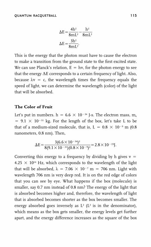
QUANTUM RACQUETBALL 115
�E�4h2
8mL2�
h2
8mL2
�E�3h2
8mL2.
This is the energy that the photon must have to cause the electron
to make a transition from the ground state to the first excited state.
We can use Planck’s relation, E � hν, for the photon energy to see
that the energy ΔE corresponds to a certain frequency of light. Also,because λν � c, the wavelength times the frequency equals the
speed of light, we can determine the wavelength (color) of the light
that will be absorbed.
The Color of Fruit
Let’s put in numbers. h � 6.6 � 10�34 J-s. The electron mass, me
� 9.1 � 10�31 kg. For the length of the box, let’s take L to be
that of a medium-sized molecule, that is, L � 0.8 � 10�9 m (0.8
nanometers, 0.8 nm). Then,
�E�3(6.6�10�34)2
8(9.1�10�31)(0.8�10�9)2�2.8�10�19J.
Converting this energy to a frequency by dividing by h gives ν �
4.25 � 1014 Hz, which corresponds to the wavelength of the light
that will be absorbed, λ � 7.06 � 10�7 m � 706 nm. Light with
wavelength 706 nm is very deep red. It is on the red edge of colors
that you can see by eye. What happens if the box (molecule) is
smaller, say 0.7 nm instead of 0.8 nm? The energy of the light that
is absorbed becomes higher and, therefore, the wavelength of light
that is absorbed becomes shorter as the box becomes smaller. The
energy absorbed goes inversely as L2 (L2 is in the denominator),
which means as the box gets smaller, the energy levels get further
apart, and the energy difference increases as the square of the box
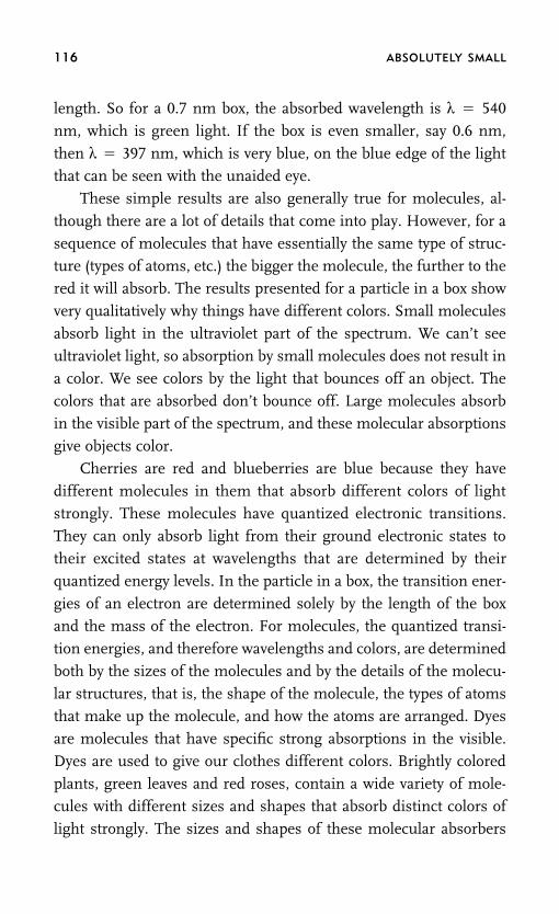
116 ABSOLUTELY SMALL
length. So for a 0.7 nm box, the absorbed wavelength is λ � 540
nm, which is green light. If the box is even smaller, say 0.6 nm,
then λ � 397 nm, which is very blue, on the blue edge of the light
that can be seen with the unaided eye.
These simple results are also generally true for molecules, al-
though there are a lot of details that come into play. However, for a
sequence of molecules that have essentially the same type of struc-ture (types of atoms, etc.) the bigger the molecule, the further to the
red it will absorb. The results presented for a particle in a box show
very qualitatively why things have different colors. Small molecules
absorb light in the ultraviolet part of the spectrum. We can’t see
ultraviolet light, so absorption by small molecules does not result in
a color. We see colors by the light that bounces off an object. The
colors that are absorbed don’t bounce off. Large molecules absorbin the visible part of the spectrum, and these molecular absorptions
give objects color.
Cherries are red and blueberries are blue because they have
different molecules in them that absorb different colors of light
strongly. These molecules have quantized electronic transitions.
They can only absorb light from their ground electronic states to
their excited states at wavelengths that are determined by theirquantized energy levels. In the particle in a box, the transition ener-
gies of an electron are determined solely by the length of the box
and the mass of the electron. For molecules, the quantized transi-
tion energies, and therefore wavelengths and colors, are determined
both by the sizes of the molecules and by the details of the molecu-
lar structures, that is, the shape of the molecule, the types of atoms
that make up the molecule, and how the atoms are arranged. Dyesare molecules that have specific strong absorptions in the visible.
Dyes are used to give our clothes different colors. Brightly colored
plants, green leaves and red roses, contain a wide variety of mole-
cules with different sizes and shapes that absorb distinct colors of
light strongly. The sizes and shapes of these molecular absorbers

QUANTUM RACQUETBALL 117
give the plants their brilliant colors. If the molecules absorb green
and red strongly, then blue will bounce off of an object, and it will
look blue. If blue and green are absorbed strongly, mainly red will
bounce off, and an object will look red. The colors that are absorbed
are determined by the quantized energy levels of the molecules in
the object.
We observe color constantly in everyday life. Color is one ofmany phenomena that we encounter that is inherently quantum
mechanical. There are many others. For example, when you turn
on an electric stove, the element gets hot. Why electricity moving
through metal produces heat (Chapter 19) is another everyday quan-
tum phenomenon. Why is carbon dioxide a greenhouse gas (Chap-
ter 17)? What is a trans fat (Chapter 16)? It is necessary to go into
the quantum mechanics of molecular structure to understand suchsystems. In the following chapters, the quantum description of
atoms and molecules will be developed and applied to a number of
common issues and problems. The necessary machinery for under-
standing atoms and molecules is developed in Chapters 9 through
14. These chapters supply a great deal of interesting information
about how atoms and molecules behave and provide the bridge be-
tween the general ideas of quantum theory that we have just devel-oped and understanding many phenomena that surround us.

9
The Hydrogen Atom:
The History
IN CHAPTER 8, WE DISCUSSED the particle in a box problem. We imag-
ined an electron confined to a very small one-dimensional box, as
shown in Figure 8.1. The particle in a box is a useful problem be-
cause the math is simple enough to find the quantized energy levels
without great difficulty. A formula was obtained that showed that
the energy states of the particle in a box come in discreet steps thatdepend on a quantum number n, where n is an integer that starts
at 1 and can take on any integer value. However, it was pointed out
that this is a very artificial example of quantum confinement. In
nature, there are no truly one-dimensional systems. Furthermore,
the walls of the box are infinitely high and completely impenetrable.
This is also physically unrealistic. As discussed in connection with
the photoelectric effect in Chapter 4, if a photon has sufficient en-ergy to overcome the binding energy of electrons to the atoms in a
piece of metal, the interaction of the photon with an initially bound
electron can eject the electron from the metal (see Figure 4.3).
However, for a number of reasons it is very useful to examine
the particle in a box. First, we found that the energy levels are quan-
118

THE HYDROGEN ATOM: THE HISTORY 119
tized (see Figure 8.6). In contrast to classical mechanics, the energy
an electron can have when confined to a box the size of an atom or
molecule is not continuous. Rather, the energy comes in discrete
steps. A photon of the right energy can excite an electron from one
energy level to another (see Figure 8.7). The energy of the photon
must match the difference between the energy of the level the elec-
tron starts in and the energy of the one it ends up in. But in contrastto real systems, no amount of energy can cause the electron to come
flying out of the box because the walls are infinitely high. This is a
way of saying that an electron would have to have infinite energy to
get out of the box. The box is an infinitely deep well and the electron
is trapped in it; no finite amount of energy can overcome the infi-
nite binding energy.
Another important feature of the particle in the box is the na-ture of the wave functions. The wave functions are probability am-
plitude waves that are related to where the electron is inside of the
box (see Figure 8.4). The square of these wavefunctions (Figure 8.5)
gives the probability of finding the electron in some region of space.
The probability amplitude waves have nodes. As the quantum num-
ber increases, the number of nodes increases, as can be seen in
Figure 8.5. Nodes are places where the probability of finding a parti-cle, such as an electron, is zero.
Atoms are real three-dimensional physical systems in contrast
to the one-dimensional particle in the box. The three-dimensional
nature of atoms is a major difference, but as discussed in Chapter
10, some of the most important features of the quantum mechani-
cal description of atoms are qualitatively similar to the particle in
the box results. Atoms have quantized energy levels. They havewavefunctions that have an increasing number of nodes as the
quantum number increases. Many other things are very different.
The quantum states of atoms have associated with them several
quantum numbers, and because atoms are three dimensional, their
wavefunctions have three-dimensional shapes. These properties of

120 ABSOLUTELY SMALL
atoms will be discussed in detail beginning in Chapter 10 with the
simplest atom, the hydrogen atom. But first, we will look at some
of the early observations that indicated that classical mechanics was
not going to be able to describe atoms.
THE SOLAR BLACK BODYRADIATION SPECTRUM
We have introduced the experimental method of spectroscopy, that
is, taking a spectrum of the light that comes out of a system or the
spectrum of the light that is absorbed by a system. A spectrum is
just a recording of the intensity of the various colors of light. We
measure the amount of light at each wavelength (color). When we
refer to colors, we don’t mean only the colors we can see, the visiblespectrum, but also longer wavelengths (lower energy), the infrared,
and shorter wavelengths (higher energy), the ultraviolet. A system
may be a container of gas molecules, the leaf of a plant, or mole-
cules in a liquid such as the molecules that make wine red. We use
complicated dye molecules to color our clothes because the size and
structure of a molecule determines which wavelengths of light it
will absorb.In Chapter 4, black body radiation was briefly discussed. A hot
object gives off light. A fairly hot piece of metal will glow red. This
can be seen in the wire elements of an electric space heater or an
electric stove. As the temperature is increased the color will move
toward the blue. It was mentioned that stars are well described as
black bodies, and the color of a star can be used to determine its
temperature. Planck developed a formula that yields the black bodyspectrum for a given temperature. Figure 9.1 shows the solar spec-
trum calculated using Planck’s formula that is the closest to the
experimentally measured solar spectrum. The frequency is plotted
in wave numbers (cm�1). Multiplying the frequency in cm�1 by the
speed of light in centimeters per second (3�1010 cm/s) gives the

THE HYDROGEN ATOM: THE HISTORY 121
FIGURE 9.1. The black body spectrum of the sun calculated using the
Planck formula for black body radiation from a hot object. The curve is
a good representation of the solar spectrum without some of the fine
details. The lower axis is the frequency in wave numbers (see text). The
top axis is the wave length in nanometers. The green light is 500 nm.
Very blue is 400 nm; very red is 666 nm. The vertical axis is the amount
of light (see text).
wavelength (nm)
frequency (cm–1)30,00020,00010,000
irra
dian
ce (
W/m
2 cm
–1)
0.02
0.08
0.06
0.04
5780 K
500 3331000 4006662000 286
frequency in Hz, the conventional frequency units. The top axis in
Figure 9.1 is the wavelength in nanometers (nm). 500 nm is green
light. 400 nm is very blue light. 666 nm is very red light. 333 nm is
in the ultraviolet region of the optical spectrum and cannot be seen
with the eye. 1000 nm is in the infrared part of the spectrum and
also cannot be seen with the eye. These wavelengths can be detected
with electronic photodetectors. Originally, they were detected with

122 ABSOLUTELY SMALL
photographic film. The vertical axis is the irradiance. It is the num-
ber of watts (joules per second) that would fall on an area of a square
meter in a little slice of frequency 1 cm�1 wide. Basically the plot is
the amount of energy per second of a particular color that falls on a
square meter.
The shape of the spectrum plotted in Figure 9.1 is almost identi-
cal to the actual solar spectrum. The calculated spectrum is obtained
by adjusting the temperature in Planck’s formula until the best
match is obtained to the experimental spectrum. The temperature
that gives the best spectrum is 5780 K, where K is the unit of tem-
perature in degrees Kelvin. This is the unit of absolute temperature
developed by William Thomson, the first Baron Kelvin (Lord Kelvin,
1824–1907). The Kelvin scale is used in physics and chemistry be-
cause it has a well-developed physical meaning for 0 K, the absolute
zero of temperature. At 0 K, all atomic motions associated with ki-
netic energy (heat), the energy of moving particles, stop. To obtain
the temperature in degrees centigrade (C) subtract 273. Then in
centigrade, the sun’s temperature is 5507 C. To convert to Fahren-
heit (F), multiply by 9/5 and add 32 to the temperature in centi-
grade. Therefore, the surface temperature of the sun is 9945 F. The
Fahrenheit temperature scale is named for Daniel Gabriel Fahren-
heit (1686–1736).
Dark Lines in the Solar Spectrum
It is remarkable that the Planck formula developed using the first
quantum concept, that the energies of electrons ‘‘oscillating’’ in a
metal are not continuous, can be used to determine the temperature
of stars. The calculated spectrum shown in Figure 9.1 is continuous
because a hot object produces a continuous distribution of colors
(energies of light). While the experimental measurement has the
shape shown in Figure 9.1, it also has some very sharp features in
it that are not part of the sun’s black body spectrum. Figure 9.2 is

THE HYDROGEN ATOM: THE HISTORY 123
FIGURE 9.2. The visible portion of the solar spectrum. The continuous
range of colors is the black body spectrum. The dark lines or bands are
colors that do not reach Earth, so they appear as colors missing from the
solar spectrum. The wavelengths of the lines and the spectrum are given
in nm, nanometers, which are billionths (10�9) meters.
656410397 434
486
400 500 600 700wavelength (nm)
an illustration of the solar spectrum with thin dark lines that repre-
sent a lack of light at certain frequencies. The spectrum shown in
Figure 9.1 is the light that comes from the sun. But the dark lines
are certain narrow bands of color that do not make it to earth. The
light is being absorbed between the sun and the earth. The lines are
called absorption lines or bands. These same lines are very promi-
nent in the spectra of light coming from stars other than our own
sun.
The same wavelengths that are seen as dark lines in the solar
spectrum can also be seen as distinct colors from an arc lamp filled
with hydrogen gas. A hydrogen arc lamp or discharge lamp is a
sealed glass cylinder filled with hydrogen gas with electrodes at ei-
ther end. When a sufficiently high voltage is connected to the lamp,
positive connected to one electrode and negative to the other elec-
trode, electricity arcs through the lamp like a small continuous
lightning bolt. The colors (wavelengths) in the visible coming out of
the lamp are the same as wavelengths of the black lines shown in
Figure 9.2.
124 ABSOLUTELY SMALL
The Hydrogen Line Spectrum
The first attempt at understanding the line spectrum of hydrogen
in the visible region was made in 1885 by the Swiss schoolteacher
and mathematician, Johann Balmer (1825–1898). Balmer noted that
the frequencies of the lines, f, in the visible part of the spectrum
were related by the formula
f �122
�1n2
.
The symbol � means proportional to, so there is a multiplicative
constant that is discussed below. In this equation, n is an integer
greater than 2, that is, 3, 4, 5, etc. The spectral lines in the visible
are called the Balmer series.
Later, lines were discovered in the ultraviolet and the infrared.These are called the Lyman series and the Paschen series, respec-
tively, after their discoverers Theodore Lyman (1874–1954), a U.S.
physicist and spectroscopist, and Louis Karl Heinrich Friedrich
Paschen (1865–1947), a German physicist. In 1888, the Swedish
physicist and spectroscopist, Johannes Rydberg (1854–1919) pre-
sented a formula that described all of the spectral lines seen in
emission from a hydrogen arc lamp or in the absorption spectrumof solar or stellar light. The Rydberg formula for the frequency of
the hydrogen atom spectral lines is
f�RH� 1n2
1
�1n2
2�.
n1 is an integer beginning at 1. n2 is another integer that must be
greater than n1. n1 � 1 gives the Lyman series. n1 � 2 gives theBalmer series. n1 � 3 gives the Paschen series. The constant, RH, is
called the Rydberg constant for the hydrogen atom. It has the value,
RH � 109,677 cm�1. Here the constant is given in wave numbers
(cm�1). When this value is used in the Rydberg formula, the fre-
quency of a spectral line determined by the integers n1 and n2 is in

THE HYDROGEN ATOM: THE HISTORY 125
wave numbers. To get it in Hz, the result is multiplied by the speed
of light in cm/s, that is, 3 � 1010 cm/s. To find the wavelength of a
spectral line, take the inverse of the frequency in wave numbers,
that is, take 1 and divide it by the frequency in wave numbers. For
example, if n1 � 2 and n2 � 3, then
f�RH�122
�132��RH�1
4�
19��1.52�104 cm�1,
the frequency in wave numbers. The inverse of this number is 6.56
� 10�5 cm � 656 � 10�9 m. 10�9 m is a nanometer, so the wave-
length is 656 nm. This is the red line in the Balmer series shown in
Figure 9.2.
In connection with Figure 8.7, we already discussed discreet
optical transitions between quantized energy levels for the particlein a box. Figure 8.7 shows transitions between the particle in a box
states for n � 1 going to n � 2 and n � 1 going to n � 3. So it
should come as no surprise that the optical transitions of the hydro-
gen atom could involve discreet frequencies that depend on inte-
gers. However, in 1888, at the time of the Rydberg formula, it was
still 12 years before the first use of the idea of quantized energy
levels by Planck to explain black body radiation, and 37 years beforetrue quantum theory took shape in 1925. The various series of spec-
troscopic lines that have energies related to integers through the
Rydberg formula can be understood as optical transitions between
discreet energy levels that are associated with the hydrogen atom. A
few of the energy levels that give rise to the Lyman series and the
Balmer series are shown in Figure 9.3. In the figure, the downward
arrows indicate the emission of light that would come from a hydro-gen arc lamp. The hydrogen atom starts in a higher energy level
and ends up in a lower energy level. Energy is conserved by the
emission of a photon. To conserve energy, the photon must have
the energy difference between the initial higher energy level and the
final lower energy level. In the Rydberg formula, the smallest value
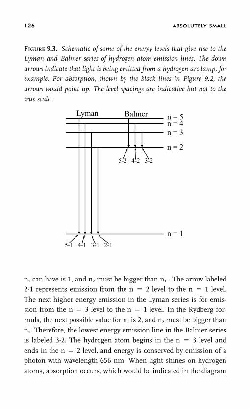
126 ABSOLUTELY SMALL
FIGURE 9.3. Schematic of some of the energy levels that give rise to the
Lyman and Balmer series of hydrogen atom emission lines. The down
arrows indicate that light is being emitted from a hydrogen arc lamp, for
example. For absorption, shown by the black lines in Figure 9.2, the
arrows would point up. The level spacings are indicative but not to the
true scale.
n = 5 n = 4 n = 3
n = 2
Lyman Balmer
5-2 4-2 3-2
n = 1 5-1 4-1 3-1 2-1
n1 can have is 1, and n2 must be bigger than n1 . The arrow labeled
2-1 represents emission from the n � 2 level to the n � 1 level.
The next higher energy emission in the Lyman series is for emis-
sion from the n � 3 level to the n � 1 level. In the Rydberg for-
mula, the next possible value for n1 is 2, and n2 must be bigger than
n1. Therefore, the lowest energy emission line in the Balmer series
is labeled 3-2. The hydrogen atom begins in the n � 3 level and
ends in the n � 2 level, and energy is conserved by emission of a
photon with wavelength 656 nm. When light shines on hydrogen
atoms, absorption occurs, which would be indicated in the diagram

THE HYDROGEN ATOM: THE HISTORY 127
by up arrows. The Balmer series absorptions are shown in Figure
9.2.
BOHR’S HYDROGEN ATOM THEORY—NOT QUITE THERE
The first detailed description of the energy levels of the hydrogen
atom was developed by Niels Bohr (1885–1962) in 1913. Bohr won
the Nobel Prize in Physics in 1922 ‘‘for his services in the investiga-
tion of the structure of atoms and of the radiation emanating from
them.’’ Bohr’s theory of the hydrogen atom is referred to as the old
quantum theory. Bohr made many advances and in fact was able
to calculate precisely the energy levels of the hydrogen atom, and
therefore obtain the Rydberg relation and predict all of the hydrogen
atom spectral lines. Bohr was also the first to propose two ideas we
have already been using. He said an atomic system can only exist
in certain states, which he called ‘‘stationary’’ states. Now, we usu-
ally refer to these as energy eigenstates. Each of these states has a
well-defined energy, E. Transitions from one stationary state to an-
other can occur by absorption or emission of light or other means
that can give or take energy from the system, and the amount of
energy must be equal to the difference in energy of the two states.
This idea is the basis for Figures 9.3 and 8.7, where the arrows
represent transitions between states that occur by absorption or
emission of light.
Bohr also put forward what came to be known as the Bohn
Frequency Rule. The frequency of light emitted or absorbed in mak-
ing a transition from an initial state with energy E1 to a final state
with energy E2 is the difference in the energies divided by Planck’s
constant, that is,
� ��E1�E2�
h.

128 ABSOLUTELY SMALL
� is the frequency and h is Planck’s constant (h � 6.6 � 10�34
J-s). The vertical lines are the absolute value. For absorption E1 is
less than E2, so E1 � E2 would be negative. The absolute value
means that you make the number positive even if the difference is
negative. The frequency, �, has to be a positive number. Multiplying
both sides by h gives E, the energy difference between the energy
levels (stationary states) as E � h�, which is the Planck relationshipthat Einstein used to explain the photoelectric effect discussed in
Chapter 4.
What is a hydrogen atom and what are the failures of the Bohr
method? A hydrogen atom is composed of two charged particles, a
proton that has a positive charge, that is, a charge of �1, and an
electron that has a negative charge, a charge of �1. When we say a
charge of 1, it actually is shorthand for the charge that is on oneproton. The charge in real units is 1.6 � 10�19 C, where C is the
Coulomb, the unit of charge. Ernest Rutherford (1871–1937) did
experiments in 1911 that showed that atoms were composed of a
small, heavy positively charged nucleus and one or more electrons
outside of the nucleus. Rutherford won the 1908 Nobel Prize in
Chemistry ‘‘for his investigations into the disintegration of the ele-
ments, and the chemistry of radioactive substances.’’ Rutherford’sfindings applied to the hydrogen atom mean that the proton is the
nucleus and a single electron is found outside the nucleus. Even for
hydrogen where the nucleus is composed of a single proton, the
nucleus is much heavier than an electron. The mass of a proton is
mp � 1.67 � 10�27 kg, while the mass of the electron is only me �
9.1 � 10�31 kg. A proton weighs about 1836 times as much as an
electron.In the Bohr model, the electron orbited the proton like a planet
orbiting the sun. The lowest energy state of the hydrogen atom, n
� 1, has the electron going around the proton in a circle. Higher
energy states of the electron, with n greater than 1, could have dif-
ferent shapes. Some were still circles, but some were ellipses. This

THE HYDROGEN ATOM: THE HISTORY 129
picture of the electron orbiting the proton should immediately set
off danger warnings based on the material covered in earlier chap-
ters. In Chapter 6, the Heisenberg Uncertainty Principle was dis-
cussed. We know that an absolutely small particle cannot have a
classical trajectory. To have a trajectory, it is necessary to know the
position and the momentum of a particle simultaneously over all
time. But the Heisenberg Uncertainty Principle says that it is notpossible to know both the position and the momentum precisely
simultaneously. The uncertainty relation states that �x�p � h/4�,
where h is Planck’s constant. Absolutely small particles are de-
scribed in terms of probability amplitude waves, not trajectories. Of
course in 1913, when Bohr came out with his mathematical treat-
ment of the hydrogen atom, the nature of absolutely small particles
was not known.The failure of Bohr’s approach became apparent when it was
applied to systems other than the hydrogen atom. While Bohr’s
method could predict very accurately the energy levels, and there-
fore the spectrum of the hydrogen atom, it could not do so for the
next simplest atom, the helium atom. Nor could it properly predict
the properties of the simplest molecule, the hydrogen molecule,
which is composed of two hydrogen atoms. The Bohr method couldnot account for the strength of the chemical bond that held the two
hydrogen atoms together to form the hydrogen molecule. Although
Bohr made giant steps in the right direction, the failures of his
approach ultimately led to the development of true quantum theory
in 1925.

10
The Hydrogen Atom:
Quantum Theory
IN 1925 SCHRODINGER AND HEISENBERG separately developed quan-
tum theory. Their two formulations are mathematically different,
but their theories are rigorous and form the underpinning of mod-
ern quantum theory. At about the same time, Dirac made major
contributions as well. First, he presented a unified view of quantum
theory that showed that the Schrodinger and Heisenberg theories,while mathematically different, were equivalent representations of
quantum mechanics. In addition, he developed a quantum theory
for the hydrogen atom that is also consistent with Einstein’s Theory
of Relativity. The formulation by Schrodinger is the most often used
to describe atoms and molecules. Therefore, most of our discus-
sions, starting with the hydrogen atom and then going on to larger
atoms and molecules, will be based on the concepts and languagethat is inherent in the Schrodinger approach.
THE SCHRODINGER EQUATION
We used a very simple but correct mathematical method for obtain-
ing the energy levels of the particle in the box and the wavefunctions,
130

THE HYDROGEN ATOM: QUANTUM THEORY 131
but the method we used is not general. For example, it cannot be
used to find the energy levels and the wavefunctions for the hydrogen
atom. In fact, the language we have been using, that is, wavefunc-
tions and probability amplitude waves, comes from Schrodinger’s
formulation of quantum theory. In 1925 Schrodinger presented what
has come to be known as the Schrodinger Equation. The Schrodinger
Equation is a complicated differential equation in three dimensions.We will not do the mathematics necessary to solve the Schrodinger
equation for the hydrogen atom or other atoms or molecules. How-
ever, we will use many of the results to learn about atoms and mole-
cules, beginning with the hydrogen atom.
The solution of the hydrogen atom problem using the Schrod-
inger Equation is particularly important because it can be solved
exactly. The hydrogen atom is a ‘‘two-body’’ problem. There are onlytwo interacting particles, the proton and the electron. The next sim-
plest atom is the helium atom, which has a nucleus with a charge
of �2 and two negatively charged electrons. This is a three-body
problem that cannot be solved exactly. In classical mechanics, it is
also not possible to solve a three-body problem. The problem of
determining the orbits of the Earth orbiting the Sun with the Moon
orbiting the Earth cannot be solved exactly with classical mechanics.However, in both quantum mechanics and classical mechanics,
there are very sophisticated approximate methods that permit very
accurate solutions to problems that cannot be solved exactly. The
fact that a method is approximate does not mean it is inaccurate.
Nonetheless, because the hydrogen atom can be solved exactly with
quantum theory, it provides an important starting point for under-
standing more complicated atoms and molecules.
WHAT THE SCHRODINGER EQUATIONTELLS US ABOUT HYDROGEN
What does the solution to the Schrodinger Equation for the hydro-
gen atom give? It gives the energy levels of the hydrogen atom, and

132 ABSOLUTELY SMALL
it gives the wavefunctions associated with each state of the hydro-
gen atom. The wavefunctions are the three-dimensional probability
amplitude waves that describe the regions of space where the elec-
tron is likely to be found. Schrodinger’s solution to the hydrogen
atom problem gives energy levels consistent with the empirically
obtained Rydberg formula. The energy levels are
En � �RH
n2,
where n is the principal quantum number. It is an integer that can
take on values �1, that is, greater than or equal to 1. The difference
in energy between any two energy levels is the Rydberg formula.
However, in the Schrodinger solution, RH is not an empirical pa-
rameter. In solving the problem, Schrodinger found the Rydberg
constant is determined by fundamental constants, with
RH � �e4
82oh2
.
h is Planck’s constant. e is the charge on the electron. o is a con-stant called the permittivity of vacuum. o � 8.54�10�12 C2/J m,
with the units Coulombs squared per Joule – meter. is the re-
duced mass of the proton and the electron. It is
�mpme
mp � me
,
where mp and me are the masses of the proton and electron, respec-
tively. The charge on the electron and the proton and their masses
were given above.While Rydberg took experimental data and developed an em-
pirical formula that described the line spectra of the hydrogen
atom, the results of Schrodinger’s solution to the hydrogen atom
problem using quantum theory are fundamentally different. We
have to spend a moment to marvel at the triumph of quantum

THE HYDROGEN ATOM: QUANTUM THEORY 133
theory that emerged in 1925. There are no adjustable parameters
in Schrodinger’s derivation of the energy levels of the hydrogen
atom. All of the necessary constants are fundamental properties
of the particles and the electrostatic interaction that attracts the
electron’s negative charge to the proton’s positive charge. Schrod-
inger did not look at the experimental data and then adjust a con-
stant, RH, until it fit the data. He set up a theoretical formalismand applied it to the hydrogen atom. The application of his theory
accurately reproduced the experimental observables, the hydrogen
atom line spectra, using only fundamental constants. In contrast
to Bohr’s theory, the Schrodinger Equation has been successfully
applied to a tremendous number of other problems including
atoms other than hydrogen and small and large molecules. As
mentioned above, for systems larger than the hydrogen atom, thatis, atoms and molecules involving more than two particles, the
Schrodinger Equation cannot be solved exactly. However, many
powerful approximation techniques have been developed that en-
able accurate solutions to the Schrodinger Equation for atoms,
molecules, and other types of quantum mechanical problems.
With the advent of computers, and the current tremendous power
of computers, it is possible to solve the Schrodinger Equation forvery large and complex molecules. As discussed in subsequent
chapters, molecules have shapes. The solutions to the Schrodinger
Equation for a molecule give its energy levels and its wavefunc-
tions. The wavefunctions provide the necessary information to de-
scribe the shapes of molecules.
THERE ARE FOUR QUANTUM NUMBERS
The energies of the different states of the hydrogen atom only de-
pend on a single quantum number, n. However, there are actually
four quantum numbers associated with electrons in atoms. These
come out of solving the hydrogen atom with quantum theory. One

134 ABSOLUTELY SMALL
of these only comes into play for atoms and molecules that have
more than one electron. In that sense, the hydrogen atom is a
special case because it has only one electron. In the hydrogen
atom, in addition to the principal quantum number n, the two
other quantum numbers are l and m. l is called the orbital angular
momentum quantum number and m is called the magnetic quan-
tum number. These two quantum numbers, when combined withn, determine how many different states are associated with a par-
ticular energy, and they determine the shapes of the wavefunc-
tions. The fourth quantum number is s. It is called the spin
quantum number. When Bohr solved the hydrogen atom problem
with old quantum theory, the electron moved in orbits that had
different energies and shapes. Schrodinger’s correct quantum
solution to the hydrogen atom gave the energies and the wavefunc-tions, which, in correspondence to Bohr’s orbits, are called ‘‘orbit-
als.’’ In discussing atoms and molecules, we often use the term
wavefunction and orbital interchangeably. The orbitals are proba-
bility amplitude waves that obey Heisenberg’s Uncertainty Princi-
ple, in contrast to Bohr’s orbits.
As stated above, the principal quantum number, n, can take on
values, n � 1, that is, 1, 2, 3, 4, etc. l can have values from 0 to n�1in integer steps. m can take on values from l to �l in integer steps.
s can only take on two values, �1/2 or �1/2. These values are sum-
marized in Table 10.1.
For historical reasons, the states with different quantum num-
bers l are given different names. An s orbital has l � 0. A p orbital
has l � 1. A d orbital has l � 2. An f orbital has l � 3. For our
discussions of all atoms, we will only need to go to f orbitals, thatis, l � 3. As shown below, these different orbital types have differ-
ent shapes.
Because the energies of the states (orbitals) of the hydrogen
atom only depend on the quantum number n, there will be more
than one state with the same energy for n � 1. For n � 1, l � 0,
THE HYDROGEN ATOM: QUANTUM THEORY 135
TABLE 10.1. Quantum Numbers.
n 1, 2, 3, 4, 5, …
0 to n – 1 (integer steps)
m + to – (integer steps)
s +1/2 or –1/2
= 0 s = 1 p
= 2 d = 3 f
calledorbitalor state
l
l
l l
l
lls only if more than one electron
and m � 0 (see the table). Therefore, there is a single orbital with
n � 1. It has l � 0, so it is referred to as the 1s orbital. The 1 is the
n value, and s means that l � 0. For n � 2, l can equal 0, giving
rise to the 2s orbital. However, for n � 2, l can also equal 1. For l
� 1, m can equal 1, 0, or �1 (see the table). l � 1 is a p orbital,
and there are three different p orbitals that can be called 2p1, 2p0,
and 2p�1. The 2 is the principal quantum number n. The p means
l � 1, and the three subscripts are the three possible m values. So
for n � 2, there are four different states.
If n � 3, then l can equal 0, to give the 3s orbital. l can also
equal 1 with m � 1, 0, and �1, to give 3p1, 3p0, and 3p�1. Inaddition, l can equal 2. For l � 2, m can equal 2, 1, 0, �1, and �2.
These are the d orbitals, 3d2, 3d1, 3d0, 3d�1, and 3d�2. There are five
different d orbitals. Therefore, for n � 3, there are nine different
states: an s orbital, three p orbitals, and five d orbitals. When n �
4, there is the 4s orbital, the three different 4p orbitals, 4p1, 4p0, and
4p�1, the five different 4d orbitals, 4d2, 4d1, 4d0, 4d�1, and 4d�2. In
addition, there are seven f orbitals, 4f3, 4f2, 4f1, 4f0, 4f�1, 4f�2, and4f�3. Therefore, for n � 4, there are a total of 16 states: an s orbital,
three p orbitals, five d orbitals, and seven f orbitals.
As mentioned above, each of the orbitals has a different shape.
It is common to rename the orbital with an indication of its shape.
For example, the three different 2p orbitals, rather than being called

136 ABSOLUTELY SMALL
2p1, 2p0, and 2p�1, are usually called 2px, 2pz, and 2py. The relation
between the subscript and the shape will become clear when the
shapes are presented.
HYDROGEN ATOM ENERGY LEVELS
Figure 10.1 shows an energy level diagram for the hydrogen atom.Levels are shown for n � 1 to 5. The spacings between the levels
are not scaled properly for clarity of presentation, but as shown, the
spacing between levels gets smaller as n increases. Also as n in-
FIGURE 10.1. Hydrogen energy level diagram. The spacings between the
levels are not to scale. The first five energy levels are shown. The energy
only depends on the principal quantum number, n. The orbitals and the
number of each type are also shown. For n � 4, there is a single s orbital,
three different p orbitals, five different d orbitals, and seven different f
orbitals. The diagram would continue with the n � 6 level. The different
levels are sometimes referred to as shells.
5s 5p� ���
5d 5f
4s 4p 4d 4f
3s 3p 3d
2s 2p
1s
1s – lowest energy level

THE HYDROGEN ATOM: QUANTUM THEORY 137
creases, the number of different states (orbitals) associated with the
particular n increases. Hydrogen is a special case because it only
has one electron. For hydrogen, all orbitals with the same n have
the same energy. As discussed in the next chapter, for atoms with
more than one electron, for a given n, orbitals with different l values
have different energies.
HYDROGEN ATOM S ORBITALS
Although the hydrogen energies only depend on the principal quan-
tum number n, l and m still play an important role. These quantum
numbers determine the shapes of the orbitals, and they determine
other aspects of the hydrogen atom’s properties. For example, the
m quantum number is called the magnetic quantum number. Thethree 2p orbitals, 2p1, 2p0, and 2p�1, differ by their m quantum
number. When the hydrogen atom is put in a magnetic field, the
energies of these three orbitals are no longer the same.
From the energy levels calculated with the Schrodinger equa-
tion (see Figure 10.1) it is clear how the empirical diagram in Figure
9.3 arises. The optical transitions seen in the line spectrum of the
hydrogen atom and described by the Rydberg formula are transi-tions between the energy levels of the hydrogen atom, energy levels
that are calculated using quantum theory with no adjustable param-
eters.
As mentioned above, the n, l, and m quantum numbers all go
into determining the shapes of the wavefunctions. The s orbitals
have l � 0. l � 0 means that the electron has no angular momen-
tum in its motion relative to the nucleus of the atom. All directionslook the same, so s orbitals are spherically symmetric three-dimen-
sional probability amplitude waves. Figure 10.2 shows schematic
representations of the 1s, 2s, and 3s orbitals (probability amplitude
waves). The darker shading indicates a greater probability of finding
the electron that distance from the center. The distances at which

138 ABSOLUTELY SMALL
FIGURE 10.2. The 1s, 2s, and 3s orbitals shown in two-dimensional rep-
resentations. These are actually spherical. Darker represents a greater
probability of finding the electron. Solid circles are distances with peaks
in the probability. Dashed circles are nodes where the probability goes to
zero. The way the orbitals are represented, they have a fairly sharp outer
edge. The orbitals are waves that become very small at large distances,
but only decay to zero as the distance from the center goes to infinity.
1s
2s
3s
the probabilities have maxima are shown by the solid circles. The
centers of the white regions in the 2s and 3s orbitals (dotted circles)
are nodes, that is, regions where the probability of finding the elec-
tron goes to zero. In going from the 1s to the 2s to the 3s, the

THE HYDROGEN ATOM: QUANTUM THEORY 139
size of the orbital becomes much larger. The electron has a greaterprobability of being found further away from the nucleus as the nquantum number increases.
The increased size of the orbitals is the reason that the energyincreases as the quantum number n increases. The formula forthe energy levels of the hydrogen atom has a negative sign in frontof it, En � �RH/n2. We use a sign convention that a lower energyis a more negative energy. The hydrogen atom is composed of aproton and an electron attracted to each other through a Coulombinteraction, that is, an electrostatic interaction. Opposite chargesattract. The proton is positively charged and the electron is nega-tively charged. When a proton and electron are infinitely far apart,they do not feel each other. There is no attraction because they areso far apart. The system has its zero of energy when the particlesare separated at infinity. The electron and proton attraction in-creases as they get closer to each other. The energy of the systemdecreases, becoming increasingly negative. The 2s orbital has theelectron further away from the proton on average than the 1s, andthe 3s orbital has the electron still further away from the proton onaverage. This is clear from Figure 10.2. As the quantum numberincreases, the energy is a smaller negative number. For larger val-ues of n, it takes less energy to separate the electron and proton,that is, to ionize the atom. Ionization is the process of pulling theelectron out of an atom so that they are no longer bound together.For n � 1, it takes an energy of RH to ionize the atom. This is theamount of energy that needs to be put into the atom to overcomethe binding of �RH. When n � 2, it only takes RH/4 to ionize ahydrogen atom. When n � 3, even less energy, RH/9, is needed toionize the atom.
SPATIAL DISTRIBUTION OF S ORBITALS
To get a better feel for the spatial distribution of the probability offinding the electron in some position, it is useful to make two types
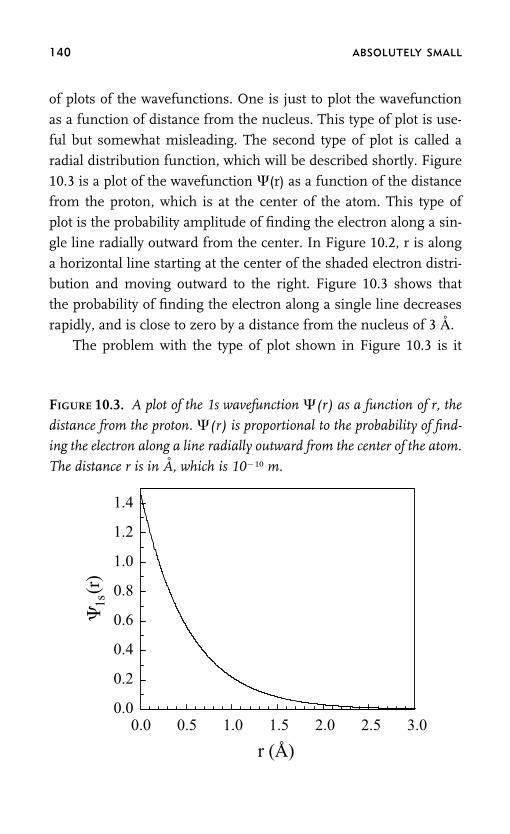
140 ABSOLUTELY SMALL
of plots of the wavefunctions. One is just to plot the wavefunction
as a function of distance from the nucleus. This type of plot is use-
ful but somewhat misleading. The second type of plot is called a
radial distribution function, which will be described shortly. Figure
10.3 is a plot of the wavefunction Ψ(r) as a function of the distance
from the proton, which is at the center of the atom. This type of
plot is the probability amplitude of finding the electron along a sin-gle line radially outward from the center. In Figure 10.2, r is along
a horizontal line starting at the center of the shaded electron distri-
bution and moving outward to the right. Figure 10.3 shows that
the probability of finding the electron along a single line decreases
rapidly, and is close to zero by a distance from the nucleus of 3 A.
The problem with the type of plot shown in Figure 10.3 is it
FIGURE 10.3. A plot of the 1s wavefunction Ψ(r) as a function of r, the
distance from the proton. Ψ(r) is proportional to the probability of find-
ing the electron along a line radially outward from the center of the atom.
The distance r is in A, which is 10�10 m.
r (Å)
0.00.0
0.2
0.4
0.6
0.8
1.0
1.2
1.4
�
0.5 1.0 1.5 2.0 2.5 3.0
1s(r
)

THE HYDROGEN ATOM: QUANTUM THEORY 141
does not account for the three-dimensional nature of the atom.
Looking at the 1s orbital in Figure 10.2, you can see that you can
find the electron at some distance from the center by moving along
a line to the right, but also along a line to the left, or up, or down.
You can also move in any diagonal direction a distance r and have
the same probability of finding the electron. Since the atom is three
dimensional, you can also move in or out of the page and find theelectron. If you want to know the probability of finding the electron
a certain distance r from the proton, you need to sum all of these
different radial directions.
What is really being asked is what is the probability of finding
the electron a certain distance from the nucleus when I add together
all possible directions? The way to state this question is, what is the
probability of finding the electron in a thin spherical shell with thespherical shell having a radius of r? As r gets bigger, the volume of
the thin spherical shell increases, which for some distance, offsets
the fact that the wavefunction is decreasing. To understand the roll
of the thin spherical shell, consider a number of hollow rubber balls
each with the same thickness rubber wall. A ball with a small radius
(small r) will have less rubber in the wall than a ball with a large
radius. If you just went in a single straight line from the center ofthe ball to the wall, and where you hit the wall you asked what is
the thickness of the rubber, it would be independent of the radius
of the ball. But it is clear that a large hollow ball has more rubber
in its wall then a small ball.
The surface area of a sphere is 4πr2, where r is the sphere’s
radius. If you multiply this by the wall thickness, you have the vol-
ume of the rubber in the ball. Now it is clear that a larger ball has alot more rubber in the wall than a small ball. If you double the
radius, the amount of rubber increases by a factor of 4. Another
important fact is that as r goes to zero, the amount of rubber in the
ball goes to zero because the surface area, 4πr2, goes to zero. Asking
if an electron is a distance r from the nucleus is like asking how

142 ABSOLUTELY SMALL
much rubber is in the wall of a ball of radius r. It is necessary to
account for the increasing surface area as the radius increases.
THE RADIAL DISTRIBUTION FUNCTION
The radial distribution function is exactly what we need to take into
account the three-dimensional nature of an atom. As r is increased
and we look in all directions to find the electron, we must include a
factor of 4�r2. The radial distribution function is a plot of the proba-
bility of finding the electron a distance r from the nucleus for all
directions. As discussed in Chapter 5, the Born interpretation of the
wavefunction says that the probability of finding a particle in some
region of space is proportional to the absolute value squared of the
wavefunction. Here we want the probability of finding the electron
in a thin spherical shell that has radius r. This is the radial distribu-
tion function, which is given by 4πr2�Ψ�2. The vertical lines mean
absolute value. For the functions we are dealing with, we just need
to square the wavefunction.
Figure 10.4 displays the radial distribution function for the 1s
state of the hydrogen atom. The distance that has the maximum
probability is not the center of the atom because the volume of the
spherical shell goes to zero as r goes to zero. The vertical line shows
the location of the maximum in the probability distribution. It is r
� 0.529 A. This is an important and interesting number. In Bohr’s
old quantum theory of the hydrogen atom, the 1s state had the elec-
tron going in a circular orbit with a radius of 0.529 A. This distance
is called the Bohr radius and is given the symbol a0. What we see
from the correct quantum mechanical treatment of the hydrogen
atom is that the electron is a probability amplitude wave with the
distance for the maximum probability equal to the Bohr radius a0.
This is not a coincidence. The Bohr radius is actually a fundamental
constant. It is given by
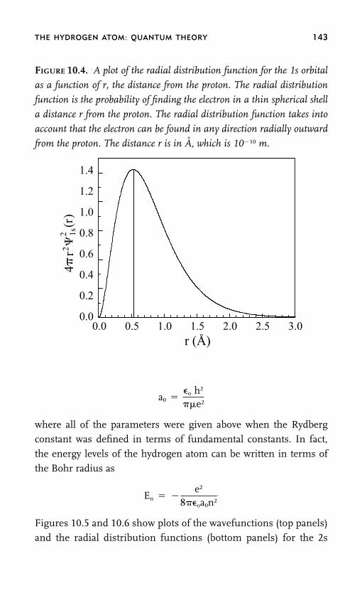
THE HYDROGEN ATOM: QUANTUM THEORY 143
FIGURE 10.4. A plot of the radial distribution function for the 1s orbital
as a function of r, the distance from the proton. The radial distribution
function is the probability of finding the electron in a thin spherical shell
a distance r from the proton. The radial distribution function takes into
account that the electron can be found in any direction radially outward
from the proton. The distance r is in A, which is 10�10 m.
r (Å)
4r2
1s(r
) 2
0.0
0.2
0.4
0.6
0.8
1.0
1.2
1.4
��
0.0 0.5 1.0 1.5 2.0 2.5 3.0
a0 �o h2
�e2
where all of the parameters were given above when the Rydbergconstant was defined in terms of fundamental constants. In fact,
the energy levels of the hydrogen atom can be written in terms of
the Bohr radius as
En � �e2
8�oa0n2.
Figures 10.5 and 10.6 show plots of the wavefunctions (top panels)
and the radial distribution functions (bottom panels) for the 2s

144 ABSOLUTELY SMALL
FIGURE 10.5. A plot of the 2s hydrogen atom wavefunction (top panel)
and the radial distribution function (bottom panel), as functions of r,
the distance from the proton. The wavefunction begins positive, goes
through a node at slightly more than 1 A (2a0), and then decays to zero.
The radial distribution function shows that the maximum probability of
finding the electron peaks at about 2.8 A, with most of the probability
between 2 and 4 A (see Figure 10.2). The distance r is in A, which is
10�10 m.
r (Å)
4r2
2s(r
) 2
0.0
0.1
0.2
0.3
–0.1
0.0
0.1
0.2
0.3
0.4
0.5
��
2s(r
) �
0 1 2 3 4 7 85 6

THE HYDROGEN ATOM: QUANTUM THEORY 145
FIGURE 10.6. A plot of the 3s hydrogen atom wavefunction (top panel)
and the radial distribution function (bottom panel), as functions of r,
the distance from the proton. The wavefunction begins positive, goes
through a node, becomes negative, goes through a second node, and be-
comes positive again. It then decays to zero. The radial distribution func-
tion shows that the maximum probability of finding the electron peaks
at about 7 A, with most of the probability between 5 and 11 A (see
Figure 10.2). The distance r is in A, which is 10�10 m.
r (Å)
0.00
0.05
0.10
0.15
–0.05
0.00
0.05
0.10
0.15
0.20
0.25
0.30
4r2
3s(r
) �
�3s
(r)
�
0 2 4 6 8 14 1610 12

146 ABSOLUTELY SMALL
and 3s orbitals. The wavefunction of the 2s orbital has a node, that
is, a place where the wavefunction is zero. Nodes were discussed
in connection with the particle in a box wavefunctions (see Figure
8.4). At a node the probability of finding a particle, in this case the
electron, is zero. The 2s wavefunction begins positive, crosses zero
at the node located at twice the Bohr radius, 2a0, and then is nega-
tive. The wavefunction then decays to zero. By 8 A the value of the
wavefunction is very small. As we have discussed in detail, the
wavefunctions are probability amplitude waves. Like other waves,
they can be positive or negative. The bottom panel of Figure 10.5
displays the 2s radial distribution function. This is the probability
of finding the electron a distance r from the nucleus. Probabilities
are always positive because they are the square of the wavefunc-
tion, which is always positive. A wave can be positive or negative,
but it makes sense that a probability is always a positive number
or zero. The radial distribution function shows that most of the
probability is between about 2 and 4 A, which also can be seen in
Figure 10.2 but not as quantitatively. The peak of the probability is
located at �2.8 A.
In Figure 10.6, it can be seen that the 3s wavefunction has two
nodes, that is, the wavefunction crosses zero twice. The hydrogen
atom wavefunctions have this in common with the particle in a box
wavefunctions (see Figure 8.4). For n � 1, there is no node. For n
� 2, there is one node. For n � 3, there are two nodes. The number
of nodes for the s orbitals is n�1. The 3s wavefunction begins posi-
tive, goes negative, and then becomes positive again. It finally de-
cays to zero, and is very small by about 16 A. The 3s radial
distribution function shows that most of the probability is relatively
far from the nucleus. The peak probability is at �7 A. Most of the
probability is between 5 and 11 A. The three radial distribution
functions shown in Figures 10.4, 10.5, and 10.6 are quantitative
plots of the information shown schematically in Figure 10.2. As the

THE HYDROGEN ATOM: QUANTUM THEORY 147
principal quantum number, n, gets larger, the s orbitals become
larger and have more nodes.
THE SHAPES OF THE P ORBITALS
For the 2s orbital, n � 2, l � 0, and m � 0. However, for n � 2,
l can also equal 1 with the associated three values of m, m � 1, 0,�1. The three different m values give rise to the three different
2p orbitals. These are shown in the energy level diagram, Figure
10.1. The three different 2p orbitals are represented schematically
in Figure 10.7. As mentioned above, because of their shapes, the
2p orbitals are usually referred to as 2pz, 2py, and 2px. Each orbital
has two lobes, a positive lobe and a negative lobe. Which lobe is
assigned positive and negative is arbitrary, but the sign mustchange because there is an angular nodal plane. The 2pz orbital
has its lobes pointed along the z axis. The nodal plane (shaded in
the figure) is the xy plane. This plane (z � 0) is a plane where the
probability of finding the electron is zero. The sign of a wavefunc-
tion changes when it passes through a node. In the 2s orbital,
there is a radial node. A radial node is a distance from the center
at which there is a node. Each p orbital has an angular node, thatis, directions (a plane) where there is a node. The 2p orbitals do
not have a radial node, but the 3p orbitals have a radial node in
addition to the angular nodal plane, and the 4p orbitals have two
radial nodes, etc.
The 2py orbital has its lobes pointed along the y axis, and its
nodal plane is the xz plane. The 2px orbital has its lobes pointed
along the x axis, and its nodal plane is the yz plane. The schematicillustrations of the 2p orbitals in Figure 10.7 are like the represen-
tations of the s orbitals in Figure 10.2. Figure 10.7 gives a feel
for the regions that have a large amount of electron probability
amplitude. However, it is important to recognize that these are
probability amplitude waves that die out smoothly away from the

148 ABSOLUTELY SMALL
nucleus. In the figure, the lobes terminate abruptly, but the wave-
functions decay at long distances in a manner similar to that
shown in Figure 10.3 for the 1s orbital. Nonetheless, Figure 10.7
is useful to get a feel for the shapes of the 2p orbitals. These
shapes will be very important when we discuss molecular bonding
and the shapes of molecules.
THE SHAPES OF THE d ORBITALS
When n � 3, l can equal 0 to give the 3s orbital. l can equal 1 with
m � 1, 0, �1 to give the three different 3p orbitals. In addition, l
can equal 2 with m � 2, 1, 0, �1, �2 to give five different 3dorbitals. These are shown in the energy level diagram, Figure 10.1.
Figure 10.8 shows the five different 3d orbitals. Like the p orbitals,
FIGURE 10.7. Schematic of the three hydrogen atom 2p orbitals, 2pz, 2py,
and 2px. Each orbital has two lobes, one positive and one negative. Each
has an angular nodal plane, that is, a plane where the probability of
finding the electron is zero. The 2pz orbital has its lobes along the z axis,
and the nodal plane is the xy plane, which is shaded. The 2py orbital has
its lobes along the y axis, and the nodal plane is the xz plane. The 2px
orbital has its lobes along the x axis, and the nodal plane is the yz plane.
The lobes in each diagram show where most of the electron probability
amplitude is located. These probability amplitude waves delay smoothly
to zero away from the nucleus (the proton) and do not stop abruptly as
in the diagrams.
2pzz
x
y+
-xynodalplane
-
2px
x
y
z
yznodalplane
+-
xznodalplane
y
x
2py
z
+
THE HYDROGEN ATOM: QUANTUM THEORY 149
the d orbitals are often given names that reflect their shapes rather
than labeling them with the quantum number, m. Four of the orbit-
als have the same basic shape. Each has four lobes and two angular
nodal planes. Two of the lobes are positive and two are negative.
When a nodal plane is crossed the wavefunction changes sign. The
fifth orbital, the dz2, has a different shape, but it still has two angular
nodal surfaces. One is the xy plane, and the other is the conicalsurface shown in the diagram. Like the p orbitals, the shaded re-
gions in Figure 10.8 indicate where most of the electron probability
amplitude is found. These probability amplitude waves go smoothly
to zero as the distance from the nucleus increases.
When n � 4, in addition to s, p, and d orbitals, l can equal 3,
which gives rise to the seven possible m values. These are the seven
f orbitals. The f orbitals have three angular nodes and very compli-cated shapes. As will be discussed in the next chapter on atoms
bigger than hydrogen, only very heavy elements have f orbitals con-
taining electrons, and the f electrons do not usually participate in
making chemical bonds. Many molecules, particularly those in
which the prime element is carbon called organic molecules, in-
volve mainly 2s and 2p orbitals. However, molecules that contain
heavier elements, such as metals, may involve d orbitals as well.In Chapter 11, we will build on our discussion of the hydrogen
atom to understand the properties of all atoms. Because these larger
atoms contain more than one electron, the fourth quantum num-
ber, s, will come into play. By applying some simple rules, we will
be able to understand many of the properties of atoms and how they
form molecules.

150 ABSOLUTELY SMALL
FIGURE 10.8. Schematics of the five hydrogen atom 3d orbitals, which
are named in relation to their shapes. Each orbital has two angular
nodes, as well as positive and negative lobes. The angular nodes are the
planes in four of the diagrams and the cones and disk in the fifth dia-
gram. When a nodal plane is crossed, the wavefunction changes sign.
The lobes in each diagram show where most of the electron probability
amplitude is located. Four of the orbitals consist of four lobes. The dz2
orbital has a different shape. It sill has two nodal surfaces, the xy plane
and the conical surfaces. These probability amplitude waves decay
smoothly to zero away from the nucleus (the proton) and do not stop
abruptly as in the diagrams.
dyzdxzdxy
x2-y2d dz2
x x x
xx
y y y
yy
zz
z z z
++
+
++
++
+
+
+-
-
- - -
-
-
-
-

11
Many Electron Atoms
and the Periodic
Table of Elements
THE PROPERTIES OF ATOMIC and molecular matter are determined by
the quantum mechanical details of the atoms that make up a sub-
stance. Common table salt is sodium chloride, NaCl. Na is the sym-
bol for the sodium atom. Sodium’s atomic number is 11. The
atomic number is the number of protons in the nucleus, that is, it
is the positive charge on the nucleus. Na has 11 protons in its nu-cleus and 11 negatively charged electrons. Chlorine (symbol Cl) has
an atomic number of 17. Cl has 17 protons in its nucleus and 17
electrons. When table salt, which is composed of little white crystals
of NaCl, is put in water, it dissolves. In water, the Na becomes the
positively charged sodium ion, Na� (sodium has lost an electron),
and the Cl becomes the negatively charged chloride ion, Cl� (chlo-
rine has gained an electron). Sodium gives up an electron to chlo-rine to form the sodium cation (positively charged ion) and the
chloride anion (negatively charged ion). The charges on the sodium
cation and the chloride anion make these ions very soluble in water.
Methane is natural gas that we burn in our gas stoves, gas
clothes dryers, and power plants. Its chemical formula is CH4. This
151

152 ABSOLUTELY SMALL
means it is composed of one carbon atom (symbol C, atomic num-
ber 6) bonded to (attached to) four hydrogen atoms (symbol H,
atomic number 1). Methane does not become ions when put in
water. In fact, it does not dissolve in water. Unless it is raised to
very high temperature as in a flame, it does not come apart at all.
Why does NaCl become separated ions, Na� and Cl�, when dis-
solved in water, while carbon always makes four chemical bondsand methane does not come apart in water to form ions? The an-
swers to these questions and many of the properties of all of the
atoms can be understood by looking at the nature of many electron
atoms and the collection of systemic information about atoms con-
tained in the Periodic Table of the Elements.
HYDROGEN IS DIFFERENT
The hydrogen atom is different from all other atoms, and the differ-
ence is highly significant. The hydrogen atom consists of a posi-
tively charged nucleus (a proton) and one negatively charged
electron. The sole electrostatic interaction is the attraction of the
electron to the proton because oppositely charged particles attract.
The next simplest atom is helium. Helium consists of a positivelycharged nucleus, with a positive charge of �2 (symbol He, atomic
number 2) and two electrons, each with a negative charge of �1.
Each electron is attracted to the nucleus. In addition, the two elec-
trons repel each other because like changes repel. The repulsion is
referred to as electron-electron repulsion. Because a hydrogen atom
has only a single electron, there is no electron-electron repulsion.
In the energy level diagram for the hydrogen atom (Figure 10.1),all of the orbitals with the same principal quantum number n have
the same energy. So the 2s and the 2p orbitals have the same en-
ergy. The 3s, 3p, and 3d orbitals all have the same energy, and so
on. The fact that energy only depends on the principal quantum
number is a result of hydrogen having a single electron. In Figures

MANY ELECTRON ATOMS 153
10.2, 10.7, and 10.8, the s, p, and d orbitals have very different
shapes. However, in hydrogen, the electron, on average, is the same
distance from the nucleus independent of the shape of the orbitals.
So an electron has the same energy whether it is in a 3s, 3p, or 3d
orbital. Why? Because the electron has the same attraction to the
nucleus when averaged over the spatial distribution given by its 3s,
3p, or 3d wavefunctions.
THE ORBITAL SHAPES MATTER FOR ATOMSLARGER THAN HYDROGEN
With more than one electron, the shapes of the orbitals matter. In
helium, if its two electrons are placed in the 2s orbital the energy is
lower than if they are placed in a 2p orbital. On average, two elec-trons in the 2s orbital are farther apart than two electrons in a 2p
orbital. Electron-electron repulsion increases the energy. Because
the two electrons are farther apart in the 2s orbital, the electron-
electron repulsion (increase in energy) is not as severe as having
the two electrons in a 2p orbital. Therefore, the 2s orbital in many
electron atoms (all atoms but hydrogen) is lower in energy than the
2p orbital. For n � 3, two electrons on average are farther apart ina 3s orbital than in a 3p orbital, and two electrons in a 3p orbital are
farther apart than if they are in a 3d orbital. So, the 3s orbital is
lower in energy than the 3p orbitals, which are lower in energy than
the 3d orbitals. However, the 3s orbital is higher in energy than the
2s orbital. On average electrons in a 3s orbital are farther from the
nucleus because the 3s orbital is larger than the 2s orbital (see Fig-
ures 10.2, 10.5, and 10.6), and therefore have a weaker attractiveinteraction with the nucleus. Less attractive interaction results in a
higher energy. The attraction to the nucleus binds the electron to
the nucleus. The sign convention is that the stronger the binding,
the lower the energy. The electron falls into the attractive well of the
positively charged nucleus. The stronger the attraction, the deeper

154 ABSOLUTELY SMALL
the electron is in the well. It will take more energy to remove the
electron from the well, that is, pull it away from the nucleus.
MANY ELECTRON ATOM ENERGY LEVELS
For a given principal quantum number n, the order of the energy is
ns � np � nd � nf. For the same type of orbital, the larger the n thehigher the energy. The important feature of many electron atoms is
that the energy depends on two quantum numbers, n and l. l is the
angular momentum quantum number that determines the shape
of the orbital. Figure 11.1 is the energy level diagram for many
electron atoms. For n � 1, there is only one type of orbital, l � 0,
an s orbital. So the 1s orbital has the lowest energy level. For n �
2, l can be 0 or 1. The l values give rise to the 2s orbital and the threedifferent 2p orbitals. With l � 1, there are three possible values of
m, m � 1, 0, �1. This is the same as in hydrogen. The big differ-
ence is that for many electron atoms, the 2s orbital is lower in en-
ergy than the 2p orbitals, as shown in Figure 11.1. For n � 3, there
is the 3s orbital, the 3p orbitals, and the 3d orbitals. As can be seen
in Figure 11.1, the 3s orbital is below (lower in energy) the 3p orbit-
als, which are below the 3d orbitals.A very important aspect of the ordering of the energy levels is
that energy levels with different n quantum numbers are inter-
spersed. Although the 3d orbitals are above the 3p orbitals, the 4s
orbital energy is actually below that of the 3d orbitals (see Figure
11.1). The ordering of the orbitals is also shown in Figure 11.1. We
see that the energy levels go 1s, 2s, 2p, 3s, 3p, 4s, 3d, 4p, 5s, 4d, and
so on. As discussed below, switching the order between the 4s andthe 3d gives rise to what is called the first transition series, and
switching the 5s and the 4d gives rise to the second transition series.
The ordering is very important in determining the properties of
various atoms. The switches in the order and the meaning of the
transition series will become clear as we discuss the Periodic Table

MANY ELECTRON ATOMS 155
FIGURE 11.1. Energy level diagram for atoms with many electrons. The
spacings between the levels are not to scale. The energy depends on the
principal quantum number, n, and the angular momentum quantum
number, l, in contrast to the hydrogen atom (Figure 10.1), where the
energy only depends on n. For n � 4, there is a single s orbital (l � 0),
three different p orbitals (l � 1), five different d orbitals (l � 2), and
seven different f orbitals (l � 3).
5s
5p
5d
4s
4p4d
4f
3s3p
3d
2s2p
1s
6s
6p7s
5s
5p
5d
4s
4p4d
4f
3s3p
3d
2s2p
1s
6s
6p7s
6d
1st trans series
2nd trans series
3rd trans series
1st inner trans series
2nd inner trans series
Order of energy levels
1s, 2s, 2p, 3s, 3p, 4s, 3d, 4p, 5s, 4d, 5p, 6s, 4f, 5d, 6p, 7s, 5f, 6d
4th trans series
5f5f
of the Elements. However, first we need to discuss how to ‘‘put’’ the
electrons into the energy levels shown in Figure 11.1.
THE THREE RULES FOR PUTTINGELECTRONS IN ENERGY LEVELS
The hydrogen atom has a nucleus with charge �1 and a single
negative electron. The helium atom has a nucleus with charge �2

156 ABSOLUTELY SMALL
and two negative electrons. Next comes the lithium atom (symbol
Li) with a �3 charge on the nucleus (atomic number 3) and three
negative electrons, which is followed by beryllium (Be) with a �4
nucleus and four negative electrons, and so on. The question is if
we have an atom with a certain number of electrons, like beryllium
with four, which energy levels do these four electrons go into? For
hydrogen, the lowest energy state is the one in which the single
electron is in the 1s orbital. If we excited the hydrogen 1s electron
to say a 2p state (adding energy by absorbing light or with an electri-
cal arc), it will fall back to the lowest energy state and conserve
energy by emitting a photon. Such photon emission from the vari-
ous energy levels of the hydrogen atom gives rise to its line spec-
trum discussed in Chapters 9 and 10. But it is not clear what to do
when there is more than one electron. Should the four electrons of
beryllium all go in the 1s orbital? It turns out that this is impossible.
Quantum theory, confirmed by countless experiments, has
given us three rules that tell us how to place the electrons into the
energy levels (Figure 11.1) to obtain the configuration of electrons
for the various atoms. We use what is called the Aufbau procedure,
that is, the build-up procedure. The three rules tell us how to place
the electrons in the energy levels in the correct order to represent
atoms. We will build up the atoms and construct the periodic table
by ‘‘putting’’ more and more electrons for bigger and bigger atoms
into the proper energy levels. Many properties of atoms, their ten-
dency to gain or lose electrons to form ions, and the number of
chemical bounds they form will be understandable from this Auf-
bau procedure, which gives rise to the form of the Periodic Table.
Rule 1—the Pauli Exclusion Principle
Rule 1 is the Pauli Exclusion Principle. It states that no two electrons
in an atom (or molecule) can have all four quantum numbers iden-
tical. There are four quantum numbers, n, l, m, and s. For hydrogen

MANY ELECTRON ATOMS 157
we only used the first three, but now s is important. s can only have
two values, s � �1/2 or �1/2. Therefore, a given orbital defined
by the quantum numbers n, l, m can have at most two electrons in
it. One of the electrons will have s � �1/2 and one will have s �
�1/2. For example, the 1s orbital has n � l, l � 0, m � 0, and s
� �1/2 or �1/2. Therefore, two electrons can go into the 1s or-
bital, one with ‘‘spin’’ �1/2 and one with spin �1/2. For the 2p
orbitals, n � 2, l � 1, m � 1, 0, �1 and s � �1/2 or �1/2. The
orbitals are px, py, and pz (see Figure 10.7). Each of these can have
two electrons in it, one with s � �1/2 and the other must have s
� �1/2. Therefore, there can be a total of six 2p electrons, two in
each of the three orbitals. 3d orbitals have quantum numbers n �
3, l � 2, m � 2, 1, 0, �1, �2, and s � �1/2 or �1/2. There are
five 3d orbitals, and two electrons can go in each (s � �1/2 or �1/
2) for a total of 10 d electrons, two in each of five orbitals. Finally,
there are seven 4f orbitals with quantum numbers, n � 4, l � 3, m
� 3, 2, 1, 0, �1, �2, �3, and s � �1/2 or �1/2. The result is a
total of 14 f electrons, two in each of seven orbitals.
When two electrons are in a single orbital, the spins are said to
be paired. An electron in an orbital (energy level) is represented by
an arrow (see Figure 11.2). The spin quantum number s � �1/2
is represented by an arrow pointing up. The spin quantum number
s � �1/2 is represented by an arrow pointing down. In any single
orbital there can be at most one up arrow and one down arrow.
Rule 2—Lowest Energy First but Don’t Violate the PauliPrinciple
Rule 2 is the orbitals are filled with electrons in order of increasing
energy. Electrons are placed in the lowest possible energy level first,
but the Pauli Principle cannot be violated. So for the helium atom
(He), both electrons can go in the 1s energy level, one with spin up
(s � �1/2) and one with spin down (s � �1/2). Three of the

158 ABSOLUTELY SMALL
FIGURE 11.2. Left-hand side: an electron represented by an arrow in an
orbital. Right-hand side: two electrons in the same orbital. The s quan-
tum numbers must be �1/2 and �1/2, represented by an up arrow
and a down arrow, to obey the Pauli Exclusion principle. The spins are
said to be paired.
spin
energy level
two electrons in an orbital
spins paired
s = +1/2 s = –1/2
quantum numbers are the same, but s is different, so the Pauli
Principle is not violated. Li is the next largest atom with three elec-
trons. The third electron cannot go in the 1s level because it would
have all four quantum numbers, n, l, m, and s, the same as one of
the other two electrons. So, the third electron must go into a higher
energy level, the 2s orbital. The 2s is the lowest possible level for
the third electron. Therefore, rule 2 dictates it will go there.
Rule 3—Hund’s Rule: Don’t Pair Spins If Possible WithoutViolating Rules 1 and 2
Rule 3 is called Hund’s Rule. Hund’s Rule states that electrons re-
main unpaired if possible when filling orbitals of identical energy.
Figure 11.3 illustrates Hund’s Rule using the 2p orbitals as an ex-
ample. The first electron, labeled 1 in the figure, is placed in the 2px
orbital. This choice is arbitrary since all three 2p orbitals have the
same energy. According to Hund’s Rule, the second electron will
go into one of the other two 2p orbitals, which have the same en-

MANY ELECTRON ATOMS 159
FIGURE 11.3. Illustration of Hund’s Rule. When filling the 2p orbitals,
electron 1 is placed in 2px, electron 2 in 2py, and electron 3 in 2pz. These
are all spin up. Electron 4 will have to have its spin down, that is, pair,
to avoid violating the Pauli Principle.
2px 2py 2pz
1 4 2 3
ergy, so that the spins are not paired. Here it is placed in the 2py
orbital. The third electron must go in the 2pz orbital, which isthe only choice that obeys Hund’s Rule as well as Rules 1 and 2.Finally, the fourth electron pairs with one of the other electrons. Asshown, it is in the 2px. It must be spin down to obey the PauliPrinciple, Rule 1.
Hund’s Rule comes about because it gives electron configura-tions with the lowest possible energy. Putting two electrons in twodifferent 2p orbitals keeps them further apart on average than put-ting them in the same orbital. The energy is lowered because keep-ing the electrons further apart reduces electron-electron repulsion.So what Hund’s Rule says in effect is to put electrons in differentorbitals if possible. While the energy reduction associated withkeeping the electrons unpaired is significant, the amount the en-ergy is lowered is not large. Therefore, it is better to pair electron 4in the 2px than to put it unpaired in the next higher energy orbital,the 3s.
THE PERIODIC TABLE OF ELEMENTS
We have laid down the rules for putting electrons in the energylevels shown in Figure 11.1. Now we will use these rules to under-

160 ABSOLUTELY SMALL
stand many properties of atoms and the Periodic Table of Elements.
In addition, these same rules will be very important in our discus-
sion of molecules presented in subsequent chapters. But first we
need to introduce the Periodic Table shown on the next page.
The Periodic Table has one box for each element. The box has
the symbol for the element, as well as its atomic number. The
atomic number is the number of positively charged protons in thenucleus. For a neutral atom (not a positively or negatively charged
ion), the atomic number is also the number of negatively charged
electrons. The form of the Periodic Table will be explained in detail
below. In the upper left corner is hydrogen, with symbol H and
atomic number 1. In the upper right corner is helium, with symbol
He and atomic number 2. Below hydrogen is lithium, with symbol
Li and atomic number 3. Many of the symbols are just abbreviationsfor the names. But this is not always true. For example, lead is
element 82 and has the symbol, Pb. Pb derives from the Latin word
for lead, plumbum. Because it is not always obvious from the symbol
what the name of the element is, Table 11.1 gives the element
names, their symbols, and their atomic numbers. The table is alpha-
betical by the element name. If you have the symbol but don’t know
the name, move down the symbol column until you find the oneyou want.
The Periodic Table (Figure 11.4) is coded for metals (white),
semimetals (semiconductors, dark gray), and nonmetals (light
gray). The semimetals are a band between the metals (most of the
elements) and the nonmetals, which are in the upper right portion
of the table. At the bottom of the table are two strips of elements
called the Lanthanide series and the Actinide series. The Lanthanideseries, usually referred to as the Lanthanides, begins with the ele-
ment La, lanthanum, and the Actinides begins with the element Ac,
actinium. These two strips go in the gap indicated in the table.
These two series of atoms, which involve the f orbitals, are placed
below the rest so that the table will not be too wide.
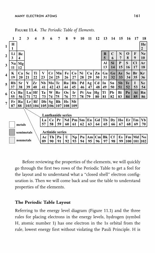
MANY ELECTRON ATOMS 161
FIGURE 11.4. The Periodic Table of Elements.
1 2 3 4 5 6 7 8 9 10 11 12 13 14 15 16 17 18
1
2
3
4
5
6
7
H1
He2
Be4
Li3
B5
C6
N7
O8
F9
Ne10
Lanthanide series
Actinide series
Na11
Mg12
Al Si P S Cl Ar 13 14 15 16 17 18
K Ca Sc Ti V Cr Mn Fe Co Ni Cu Zn Ga Ge As Se Br Kr 19 20 21 22 23 24 25 26 27 28 29 30 31 32 33 34 35 36
Rb Sr Y Zr Nb Mo Tc Ru Rh Pd Ag Cd In Sn Sb Te I Xe 37 38 39 40 41 42 43 44 45 46 47 48 49 50 51 52 53 54 Cs Ba Lu Hf Ta W Re Os Ir Pt Au Hg Tl Pb Bi Po At Rn 55 56 71 72 73 74 75 76 77 78 79 80 81 82 83 84 85 86 Fr Ra Lr Rf Db Sg Bh Hs Mt 87 88 103 104 105 106 107 108 109
La Ce Pr Nd Pm Sm Eu Gd Tb Dy Ho Er Tm Yb57 58 59 60 61 62 63 64 65 66 67 68 69 70
Ac Th Pa U Np Pu Am Cm Bk Cf Es Fm Md No89 90 91 92 93 94 95 96 97 98 99 100 101 102
metals
semimetals
nonmetals
Before reviewing the properties of the elements, we will quickly
go through the first two rows of the Periodic Table to get a feel for
the layout and to understand what a ‘‘closed shell’’ electron config-
uration is. Then we will come back and use the table to understand
properties of the elements.
The Periodic Table Layout
Referring to the energy level diagram (Figure 11.1) and the three
rules for placing electrons in the energy levels, hydrogen (symbol
H, atomic number 1) has one electron in the 1s orbital from the
rule, lowest energy first without violating the Pauli Principle. H is
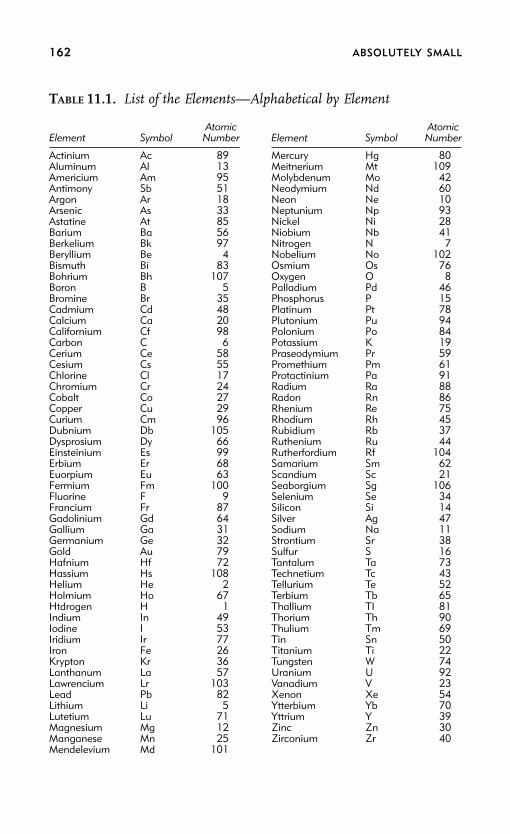
162 ABSOLUTELY SMALL
TABLE 11.1. List of the Elements—Alphabetical by Element
AtomicElement Symbol Number
Actinium Ac 89Aluminum Al 13Americium Am 95Antimony Sb 51Argon Ar 18Arsenic As 33Astatine At 85Barium Ba 56Berkelium Bk 97Beryllium Be 4Bismuth Bi 83Bohrium Bh 107Boron B 5Bromine Br 35Cadmium Cd 48Calcium Ca 20Californium Cf 98Carbon C 6Cerium Ce 58Cesium Cs 55Chlorine Cl 17Chromium Cr 24Cobalt Co 27Copper Cu 29Curium Cm 96Dubnium Db 105Dysprosium Dy 66Einsteinium Es 99Erbium Er 68Euorpium Eu 63Fermium Fm 100Fluorine F 9Francium Fr 87Gadolinium Gd 64Gallium Ga 31Germanium Ge 32Gold Au 79Hafnium Hf 72Hassium Hs 108Helium He 2Holmium Ho 67Htdrogen H 1Indium In 49Iodine I 53Iridium Ir 77Iron Fe 26Krypton Kr 36Lanthanum La 57Lawrencium Lr 103Lead Pb 82Lithium Li 5Lutetium Lu 71Magnesium Mg 12Manganese Mn 25Mendelevium Md 101
AtomicElement Symbol Number
Mercury Hg 80Meitnerium Mt 109Molybdenum Mo 42Neodymium Nd 60Neon Ne 10Neptunium Np 93Nickel Ni 28Niobium Nb 41Nitrogen N 7Nobelium No 102Osmium Os 76Oxygen O 8Palladium Pd 46Phosphorus P 15Platinum Pt 78Plutonium Pu 94Polonium Po 84Potassium K 19Praseodymium Pr 59Promethium Pm 61Protactinium Pa 91Radium Ra 88Radon Rn 86Rhenium Re 75Rhodium Rh 45Rubidium Rb 37Ruthenium Ru 44Rutherfordium Rf 104Samarium Sm 62Scandium Sc 21Seaborgium Sg 106Selenium Se 34Silicon Si 14Silver Ag 47Sodium Na 11Strontium Sr 38Sulfur S 16Tantalum Ta 73Technetium Tc 43Tellurium Te 52Terbium Tb 65Thallium TI 81Thorium Th 90Thulium Tm 69Tin Sn 50Titanium Ti 22Tungsten W 74Uranium U 92Vanadium V 23Xenon Xe 54Ytterbium Yb 70Yttrium Y 39Zinc Zn 30Zirconium Zr 40

MANY ELECTRON ATOMS 163
in the upper left corner of the Periodic Table. It is the first element
in row 1. The next element is helium (He, 2). It has two electrons
in the 1s orbital with opposite spins (arrow up and arrow down, as
shown in Figure 11.2). This configuration obeys the Pauli Principle
and the lowest energy first rule, which overrides Hund’s Rule be-
cause it would take too much energy to put the second helium elec-
tron in the 2s energy level (see Figure 11.1). He is in the upper rightcorner of the Periodic Table; it completes the first row. The first row
has the two elements, H and He, with electrons in the n � 1 level.
The rows are also referred to as shells. Helium completes the first
shell. We say that He has a closed shell configuration because it is
the largest element with n � 1.
The next element is lithium (Li, 3). It has three electrons. The
first two electrons go into the 1s energy level obeying the lowestenergy first rule. The third electron cannot go into the 1s orbital
because that would violate the Pauli Principle. So the third electron
goes in the 2s orbital. Li is below H in the Periodic Table. H is the
first element with an electron in the n � 1 shell. Li is the first
element in the second row, the n � 2 shell. The next element is
beryllium (Be, 4). The fourth electron also goes into the 2s orbital.
This is the lowest energy state, and it does not violate the PauliPrinciple. The next element is boron (B, 5) with five electrons. The
fifth electron cannot go in the 2s orbital because that would violate
the Pauli Principle, which states that no more than two electrons
can go into a single orbital and those two must have opposite spins
(spin quantum number, s � �1/2 and s � �1/2). So, the fifth
electron goes into a 2p orbital. It doesn’t matter which 2p orbital.
Following Figure 11.3, we will put it in the 2px orbital. There is agap in the table between Be and B. The reason for this will be clear
when we discuss the fourth row below. The next element is carbon
(C, 6) with six electrons. Now Hund’s Rule comes into play, and we
put the sixth electron into the 2py orbital following the layout of
Figure 11.3. Nitrogen is next (N, 7). Following Hund’s Rule, the
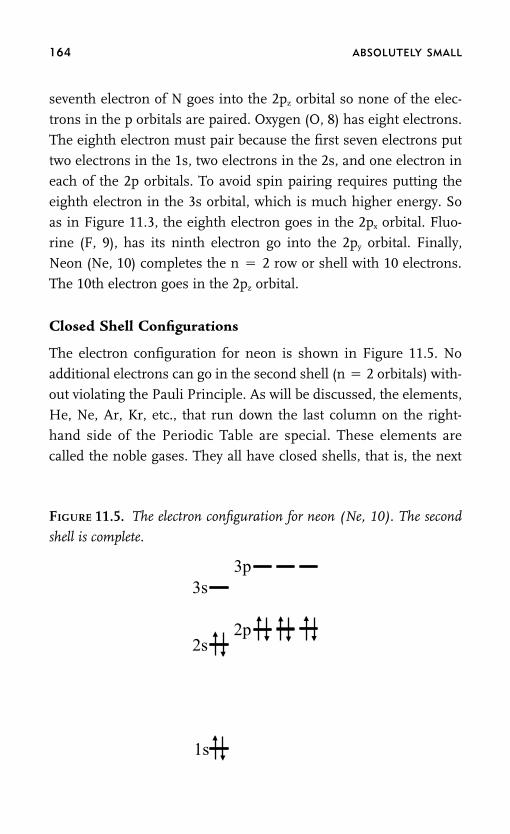
164 ABSOLUTELY SMALL
seventh electron of N goes into the 2pz orbital so none of the elec-
trons in the p orbitals are paired. Oxygen (O, 8) has eight electrons.
The eighth electron must pair because the first seven electrons put
two electrons in the 1s, two electrons in the 2s, and one electron in
each of the 2p orbitals. To avoid spin pairing requires putting the
eighth electron in the 3s orbital, which is much higher energy. So
as in Figure 11.3, the eighth electron goes in the 2px orbital. Fluo-rine (F, 9), has its ninth electron go into the 2py orbital. Finally,
Neon (Ne, 10) completes the n � 2 row or shell with 10 electrons.
The 10th electron goes in the 2pz orbital.
Closed Shell Configurations
The electron configuration for neon is shown in Figure 11.5. No
additional electrons can go in the second shell (n � 2 orbitals) with-
out violating the Pauli Principle. As will be discussed, the elements,
He, Ne, Ar, Kr, etc., that run down the last column on the right-hand side of the Periodic Table are special. These elements are
called the noble gases. They all have closed shells, that is, the next
FIGURE 11.5. The electron configuration for neon (Ne, 10). The second
shell is complete.
3s3p
2s2p
1s

MANY ELECTRON ATOMS 165
element with one more electron goes into an orbital with the n
quantum number one unit larger, which is substantially higher in
energy.
Atoms Want to Form Closed Shell Configurations
We are now ready to use the energy level diagram, Figure 11.1, and
the three rules for placing electrons in the energy levels to under-
stand the structure of the Periodic Table and the properties of the
atomic elements. The following chapters investigate in considerable
detail what holds atoms together to make molecules. However, a
great deal can be learned from an amazingly simple rule: Atoms will
gain or lose electrons to obtain the nearest closed shell configuration. The
closed shell electron configurations are the configurations of the
noble gases that comprise the right-hand column of the Periodic
Table. A closed shell configuration is particularly stable. The noble
gases, also called the inert gases, have the closed shell configuration
and are essentially chemically inert. The noble gases with small
atomic numbers, helium, neon, and argon, do not form chemical
compounds at all. The higher atomic number noble gases can be
forced to form a small number of compounds under specialized
conditions. Atoms other than the noble gases change in ways so
that they achieve a stable closed shell electron configuration.
There are two ways that an atom can change the number of
electrons it has to achieve a closed shell configuration. The first is
to become a positive ion (cation) or negative ion (anion). The atom
gives up one or more electrons and becomes positively charged (cat-
ion), or the atom takes on extra electrons, and becomes negatively
charged (anion). The other is for an atom to share electrons with
one or more other atoms. When two or more atoms share electrons,
it is as if each atom has the electrons it needs. So an atom with
fewer electrons than the number needed for the next closed shell
configuration obtains the correct number, but so do the other atoms
166 ABSOLUTELY SMALL
that are involved in the sharing. When atoms share electrons to get
to the next closed shell number of electrons, the sharing holds the
atoms together. The sharing makes the energy of the combined
atoms lower than the energies of the individual open shell atoms.
The lowering of the energy bonds the atoms together. This type of
chemical bond is called a covalent bond. Covalent bonds are respon-
sible for most of chemistry. The detailed nature of the covalent bond
is presented for the simplest molecule, the hydrogen molecule in
Chapter 12, and more complex molecules are discussed in subse-
quent chapters.
The Properties of Atoms
To begin our discussion of the properties of atoms based on the
Periodic Table, we start with hydrogen. As usual, hydrogen is spe-
cial because it only has one electron and is the first element in the
Periodic Table. For the first row of the periodic table, helium has a
closed shell with two electrons in the 1s orbital. Hydrogen can ob-
tain the helium closed shell configuration by sharing with another
atom to pick up an electron. For example, one H atom can share
electrons with a second H atom, to form the hydrogen molecule.
The symbol for the hydrogen molecule is H2. The subscript tells
how many of a given type of atom are in a molecule. Because of the
sharing, each H atom feels as if it has two electrons, the helium
closed shell configuration. As we will see, hydrogen can form other
molecules, but because it only needs one electron to get to the he-
lium closed shell configuration, it only makes one chemical bond.
Helium has the closed shell. It does not make any chemical bonds.
There are no molecules with a helium atom in them. Exactly why
this is true is described in detail in Chapter 12. Helium completes
the first shell.
The next atom is lithium, Li, which is directly below H on the
periodic table. Li can obtain the helium closed shell configuration

MANY ELECTRON ATOMS 167
by giving up an electron. Therefore, Li forms �1 ions, Li�1. A solid
piece of Li is a metal. Metals can conduct electricity, which means
electrons can move easily from one atom to another. The nature of
metals and electrical conductivity will be discussed in Chapter 19.
Metals have the property that as single atoms they can easily give up
one or more electrons. The electron Li loses has to go somewhere. It
will go to another atom that wants an electron to form a negativeion. So to form Li�1, Li needs a partner (see the discussion below
when we get to the other side of the Periodic Table). The next ele-
ment is beryllium. Beryllium will give up two electrons to go back
to the He closed shell configuration. Therefore, Be will form �2
ions, Be�2. Because Be can readily give up electrons, solid beryllium
is a metal. The next element is boron. Boron can lose three electrons
to go back to the He closed shell configuration. Therefore, it forms�3 ions, and it is a metal.
Now things change. The next element is carbon. Carbon would
have to give up four electrons to go back to the He configuration,
but it can also gain four electrons to go to the next closed shell
configuration, that of neon. As shown in Figure 11.5, Ne has a
closed shell configuration, with the second shell filled. It has two
electrons in the 1s orbital and then has the n � 2 shell filled withtwo electrons in the 2s and six electrons in the three 2p orbitals.
Rather than losing so many electrons to go back to the He configu-
ration, C goes forward to the Ne configuration, picking up four elec-
trons by making four covalent bonds. For example, methane
(natural gas) is the molecule CH4. Each H is bonded to the central
C. The carbon shares four electrons, one from each of the hydro-
gens, so C obtains the Ne closed shell configuration by sharing fourelectrons with the four H atoms. Each H shares one electron with
the C, so each H picks up one electron to have the He closed shell
configuration. This is very important. Through covalent bonds (elec-
trons sharing), each atom obtains a closed shell configuration. An-
other exceedingly important fact is that C always makes four bonds

168 ABSOLUTELY SMALL
because it needs to share four electrons to get to the Ne configura-
tion. This fact is fundamental to organic chemistry and to the chem-
istry of life. The bonding and chemistry of carbon will be discussed
extensively in subsequent chapters
The next element is nitrogen. N needs three electrons to get to
the Ne configuration, so it makes three covalent bonds. For exam-
ple, it will combine with H to make NH3, which is ammonium.Oxygen needs two electrons to get to the Ne closed shell configura-
tion, so it forms two bonds and, for example, makes H2O, water. So
from these simple considerations we can understand the sequence
of compounds, CH4, NH3, and H2O. Bonding involving C, N, and
O will be discussed in later chapters to understand molecules in-
volving these atoms, but they will always make 4, 3, and 2 bonds,
respectively.The next atom is fluorine. Fluorine is only one electron away
from the Ne closed shell. It only needs one electron to obtain the
Ne configuration. It has such a strong affinity for an electron that it
tends to form the negative ion F�1 by picking up an electron. The
electron has to come from somewhere, and F forms what are gener-
ically called salts. For example, LiF is a white crystalline solid. In
the crystal, an Li that wants to give up an electron to obtain the Heconfiguration gives its electron to an F. The result is that an LiF
crystal is composed of Li�1 ions and F�1 ions. The Li�1 ions have
the He closed shell configuration, and the F�1 ions have the Ne
closed shell configuration. LiF crystals, like all salts, dissolve readily
in water. The crystal is held together by electrostatic interactions.
The positive and negative ions attract each other. They are arranged
in the crystal in such a way that the attractive interactions amongcations and anions overcome the repulsive interactions of the cat-
ions with other cations and the anions with other anions. Water can
surround both positive and negative ions in a way that makes the
energy of the total system, water surrounding cations and anions,
lower than that of an LiF crystal sitting in water. This is called solva-

MANY ELECTRON ATOMS 169
tion. Water can solvate ions, so ionic crystals like LiF dissolve in
water. Solvation is discussed in Chapter 15.
F will form salts with atoms on the left side of the Periodic
Table, which want to give up electrons to obtain a closed shell con-
figuration. In LiF, F gains an electron and Li loses an electron. F
can also obtain the closed shell Ne configuration by making cova-
lent bonds under some circumstances. As discussed below, it cancombine with sulfur (S) to form the compound, SF2.
After F comes Ne in the periodic table. It has a closed shell (see
Figure 11.5). Ne does not want to gain or lose electrons. It does not
form chemical compounds. Ne completes the second row of the
Periodic Table. After Ne is sodium. Sodium is one electron (3s) past
the Ne configuration. Like Li directly above it, Na will readily give
up an electron to form the cation, Na�1. It does this to obtain the Neconfiguration. Solid sodium is a metal that can conduct electricity
(electrons) because its 3s electron is not tightly bound. Like LiF,
NaF is a salt that will readily dissolve in water. Next comes magne-
sium. Mg will give up two electrons to obtain the Ne closed shell
configuration, forming Mg�2 ions. It is a metal that conducts elec-
tricity because it can readily give up its two 2s electrons. It will make
salts of the form, for example, MgF2. This means the crystal has twofluorine anions for every magnesium �2 cation. MgF2 will readily
dissolve in water. After Mg comes aluminum. Solid Al is a metal.
Al will form Al�3 cations.
As with carbon in the second row, things change with silicon.
Si will make four covalent bonds to share (effectively gain) four
electrons to obtain the argon closed shell configuration (see the Pe-
riodic Table). For example, it will form SiH4. Phosphorous willmake three covalent bonds to obtain the Ar configuration, for exam-
ple, PH3, and S will make two covalent bonds to get to the Ar closed
shell configuration. It will form the compound H2S, which is hydro-
gen sulfide, the very smelly and poisonous gas that gives rotten eggs
their smell. As mentioned above, S can also make covalent bonds with
170 ABSOLUTELY SMALL
F, to form SF2. After S comes chlorine. Like F, which only needs
one electron to obtain the Ne closed shell configuration, Cl only
needs one electron to obtain the Ar closed shell configuration, so it
tends to form Cl�1 by gaining an electron. All of the elements in
the column next to the noble gases, the second column from the
right in the Periodic Table, form �1 anions. These elements (F, Cl,
Br, I, At) are called the halogens. This brings us to common table
salt, sodium chloride, NaCl, which is a crystalline solid composed
of Na�1 and Cl�1. Like LiF, NaCl can dissolve in water because the
cations and anions can be solvated by the H2O molecules. This is in
contrast to methane, CH4, which does not dissolve in water. The
carbon and the hydrogens close their shells by sharing electrons
with each other to form covalent bonds. If methane separates into
pieces, the atoms will no longer have closed shells. This is different
than an NaCl crystal, which can come apart into Na�1 and Cl�1.
Both the cation and anion have closed shells. Molecules that are
only composed of carbon and hydrogen, like oil, gasoline, and meth-
ane, are called hydrocarbons. They do not dissolve in water. Hydro-
carbons are discussed in Chapters 14, 15, and 16. After Cl is Ar.
Argon has a closed shell, as shown in Figure 11.6. It has 18 elec-
trons, two in the 1s, two in the 2s, six in the three 2p orbitals, two
in the 3s, and six in the three 3p orbitals. Ar is an inert gas. It does
not form chemical compounds.
Going Down a Column, Atoms Get Bigger
Going down a column in the Periodic Table, the atoms get bigger.
So, Li is bigger than H, Na is bigger than Li, and so forth. Two
considerations explain this. First, the additional electrons go into
orbitals with a larger principal quantum number, n. H has a 1s
electron, Li has a 2s electron, and Na has a 3s electron. Looking at
Figures 10.2 through 10.6, which are for hydrogen, you can see that
the 3s wavefunction is much bigger than the 2s, which is much

MANY ELECTRON ATOMS 171
FIGURE 11.6. The electron configuration for argon (Ar, 18). The third
row is complete.
4s
4p
3s3p
3d
2s2p
1s
4s
4p
3s3p
3d
2s2p
1s
bigger than the 1s. However, as we go down a column, the positive
nuclear charge also increases. The nuclear charge is the same as theatomic number, which is given for each atom in the Periodic Table
as well as in the List of Elements. The increased nuclear positive
charge pulls the negatively charged electrons in closer. This in-
creased attraction is not sufficient to offset the fact that going down
a column puts electrons in orbitals with larger principal quantum
numbers (n). The increase in size with n wins out over the in-
creased nuclear attraction for the electrons, resulting in largeratoms as you move down a column.
Going Left to Right Across a Row, Atoms Get Smaller
As you go along a row from left to right, the atoms get smaller. So
Be is smaller than Li, B is smaller than Be, C is smaller than Be,
etc. The reduction in size occurs because all of the atoms have the
same principal quantum number n, but the nuclear charge in-

172 ABSOLUTELY SMALL
creases. Again two phenomena are playing off against each other.
The positive nuclear charge increases as you move to the right along
a row. The increased positive charge will pull the electrons in closer
to the nucleus. However, there are also more electrons. The nega-
tive electrons repel each other (electron-electron repulsion). To re-
duce the electron-electron repulsion, the electron cloud (probability
amplitude wave) gets larger. The positive charge is at the center,
pulling all of the electrons in. But the negative electron cloud is
spread out around the nucleus. Speaking very classically, at a given
instant, the electrons on one side of the atom don’t feel (aren’t re-
pelled by) the electrons all the way on the other side of the atom as
much as they are attracted to the nucleus at the center. So the attrac-
tion wins, and the atoms get smaller as you move along a row from
left to right.
The First Transition Series
Now we are at the fourth row. After Ar, the first element in the
fourth row is potassium, K. K has one 4s electron past the Ar con-
figuration. By now it should be clear that potassium will form K�1
ions so that it can obtain the Ar closed shell configuration. Solid K
is a metal that conducts electricity. The salt KCl is a small compo-
nent of sea salt, which is mainly NaCl. KCl dissolves in water to
give the ions K�1 and Cl�1. Next to K is calcium, Ca. Ca has two 4s
electrons past the Ar configuration. It is a metal that forms Ca�2
ions, giving up its two 4s electrons to obtain the Ar closed shell
configuration. It will form salts like CaCl2, which readily dissolve in
water to give a calcium �2 cation and two chloride anions.
Now things change again in a big way. The energy level diagram
for many electron atoms (Figure 11.1) shows that the 3d orbitals are
above the 4s orbitals in energy, but they are below the 4p orbitals.
As mentioned earlier in this chapter, the interposition of the 3d
orbitals between the 4s and the 4p orbitals gives rise to the first
MANY ELECTRON ATOMS 173
transition series in the Periodic Table. There are five 3d orbitals.
The Pauli Principle states that there can be at most two electrons in
an orbital. Then there can be 10 electrons in the five 3d orbitals,
resulting in the 10 transition metals, scandium through zinc (see
the Periodic Table). So after Ca come 10 elements that arise from
filling the 3d orbitals. All of these are metals. Many of them are very
common metals that we are familiar with in everyday life, such asiron (Fe), copper (Cu), nickel (Ni), zinc (Zn), and chromium (Cr).
They can readily form ions. The first two elements in a row, such
as K and Ca or Na and Mg, always form cations with a particular
charge, �1 for the first column (Na�1 and K�1) and �2 for the
second column (Mg�2 and Ca�2). However, the transition metals
can form a variety of cations. They are said to have various oxidation
states. When a metal loses an electron it is said to be oxidized. Theoxidation state is the number of electrons it loses.
Consider iron. It can form the oxidation states �2 and �3, that
is, it forms the cations Fe�2 and Fe�3. Fe�2 is readily understand-
able. Fe can lose the two 4s electrons just like Ca to make the �2
oxidation state. In addition, Fe has six 3d electrons. Hund’s Rule
says that electrons will stay unpaired if possible. Five electrons can
go into one of each of the five 3d orbitals. This half-filled configura-tion is particularly stable. Iron is one 3d electron past the half-filled
3d orbitals, so it will readily lose a 3d electron in addition to the two
4s electrons to give an oxidation state of �3. So Fe can form salts
like FeCl2 and FeCl3.
In addition to giving rise to the first transition series (first group
of transition metals), the 3d electrons are involved in another im-
portant molecular phenomenon. We discussed that oxygen willform two covalent bonds (share two electrons with other atoms) to
obtain the Ne configuration. An example is water, H2O. Sulfur,
which is directly below oxygen, forms H2S, analogous to H2O. How-
ever, it can also form SF6 through involvement of the 3d orbitals,
which are close in energy to the 3p orbitals. There is no equivalent

174 ABSOLUTELY SMALL
for oxygen because the first set of d orbitals, the 3d’s, are much
higher in energy than the 2s and 2p orbitals that are involved in
bonding in the second row of the Periodic Table.
After the first series of transition metals are completed by filling
the 3d orbitals, the next element is gallium (Ga). Ga is a metal, and
like aluminum, it will form �3 ions. The configuration in which
the 3d orbitals are completely filled is very stable, so Ga only forms
�3 cations. The stability of the filled 3d orbitals can also be seen in
zinc. Zn only forms �2 ions by losing the two 4s electrons. Follow-
ing Ga are germanium (Ge), arsenic (As), and selenium (Se), which
tend to form four, three, and two covalent bonds, respectively, to
obtain the krypton (Kr) closed shell configuration. Like the elements
immediately above Ge, As, and Se, additional bonds can be formed
by involving the 4d electrons, which are very close in energy to the
4p orbitals. The next element is bromine, which is a halogen, and
forms a �1 anion to obtain the Kr closed shell configuration. Fi-
nally, the row ends with krypton, which has a closed shell.
Larger Atoms and the Lanthanides and Actinides
The elements in the fifth row of the Periodic Table follow the same
trends as those in the fourth row. The fifth row has the second
series of transition metals. The elements in the sixth and seventh
rows behave like those in the fourth and fifth rows except that they
also have the lanthanides (first inner transition series) and actinides
(second inner transition series). These come about by filling the 4f
and 5f orbitals (see the many electron atom energy level diagram,
Figure 11.1). The 4f (lanthanides) and 5f (actinides) orbitals (n � 4
and 5) are spatially much smaller than the 6s and 6p and 7s and 7p
orbitals (n � 6 and 7) that are filled in the sixth and seventh rows
because the principal quantum numbers, n, are smaller. The outer-
most electrons (largest principle quantum number) determine the

MANY ELECTRON ATOMS 175
chemical properties of atoms, that is, how many covalent bonds
they make or what types of ions they form. Therefore, the 4f and 5f
orbitals do not influence the chemical properties significantly. The
lanthanides begin with lanthanum (La). The 4f energy levels are
very close in energy to the 5d levels (see Figure 11.1). La comes after
barium (Ba), which has two electrons in the 6s orbital. La has one
more electron, which is actually in a 5d orbital. After La the 4f orbit-
als are filled. Lutetium (Lu, element 71) begins the third transition
metal series. It has two electrons in the 6s orbital, 14 electrons in
the 4f orbitals, and one electron in a 5d orbital. All of the lanthan-
ides have chemical properties that are quite similar to La and Lu. In
the same manner, the actinides begin with actinium (Ac). After fill-
ing the 5f orbitals with 14 electrons, lawrencium (Lr, the manmade
element 103) begins the fifth transition metal series. All of the actin-
ides have chemical properties that are very similar to Ac and Lr.
Most Elements Are Metals
The Periodic Table is color coded (shaded in Figure 11.4), with the
elements divided into metals, semimetals (semiconductors), and
nonmetals (insulators). (A detailed quantum theory explanation of
why materials are metals, semiconductors, or insulators is pre-
sented in Chapter 19.) The Periodic Table shows that the vast ma-
jority of elements are metals. It is easy to see why this is. The left
two columns are metals because they are comprised of elements
that are either one or two s electrons past the previous noble gas
closed shell configuration. They can readily give up these electrons
to fall back to the closed shell configuration. Therefore, in solid
form, it is easy to move electrons, and the solids are electrical con-
ductors. Adding d electrons in the transitions series doesn’t elimi-
nate the ability of an element to give up its outermost (highest n) s
electrons. The d electrons only add more electrons that can be lost

176 ABSOLUTELY SMALL
under the right circumstances. Adding f electrons doesn’t change
things. Therefore, in addition to the two left-hand columns of ele-
ments, all of the transition series of elements are metals, usually
called the transition metals. The inner transition series (addition of
f electrons) are also metal. The elements that can lose three elec-
trons to fall back to the previous closed shell configuration, like
aluminum, are also metals. All of these together comprise most ofthe elements. The nonmetals are the group of elements in the
upper right triangle-like block of elements in the Periodic Table.
Some of these are the elements that tend to form covalent bonds
by sharing electrons. They do not want to give up electrons. The
halogens want to gain electrons or form covalent bonds. And the
noble gases, by and large, do not want to gain or lose electrons or
form covalent bonds. Therefore, all of these are nonmetals. If theyare solids, the atoms do not want to give up electrons, a property
necessary to conduct electricity. They are insulators. The small
group of elements that form a diagonal block near the right side
of the Periodic Table are semimetals or semiconductors. They are
between the true metals and the nonmetals. Under some circum-
stances, they will conduct electricity. Silicon is the most well known
and most technologically important of these semiconductors. Sili-con is used in all of the microelectronics in our computers and
other digital devices. In Chapter 19, we will discuss the differences
among metals, insulators, and semiconductors, using the ideas of
molecular orbital theory, which will be introduced in Chapter 12
and expanded on in the following chapters.
In this chapter, we used the many electron energy level diagram
(Figure 11.1), and the rules for filling the atomic orbitals (the PauliPrinciple, lowest energy first if possible, Hund’s Rule) to discuss
the Periodic Table. It was shown that very simple considerations can
go a long way toward understanding the properties of the atomic
elements and some aspects of chemical bond formation to make
molecules. However, we did not use our ideas of quantum theory
MANY ELECTRON ATOMS 177
to discuss why chemical bonds should form and properties of mole-
cules, such as their shapes, that arise from quantum considerations.
We will begin the explication of the quantum theory of molecules
with the simplest molecule, the hydrogen molecule H2, in Chapter
12.

12
The Hydrogen Molecule
and the Covalent Bond
ONE OF THE GREAT TRIUMPHS of quantum mechanics is the theoretical
explanation of the covalent bond. Two types of interactions hold
atoms together, covalent bonds and ionic bonds. Ionic bonds are
the type that occurs in a sodium chloride (NaCl) crystal. We know
from Chapter 11 and our discussion of the Periodic Table that this
salt crystal is composed of sodium cations, Na�1, and chlorideanions, Cl�1. The ions in the crystal are held together by electro-
static interactions. Opposite charges attract. There are some compli-
cations because like charges repel, but it is possible to show that the
attractions of the oppositely charged ions overcome the repulsions
of the like charged ions. Such electrostatic interactions can be ex-
plained quite well with classical mechanics, although quantum the-
ory is still needed to explain many properties in detail.In contrast to ionic solids that are held together by electrostatic
interactions, classical mechanics cannot explain the covalent bond.
We saw in Chapter 11 that a hydrogen atom will tend to form one
covalent bond with another atom to share one electron. This sharing
brings the H atom to the helium closed shell configuration. But
178

THE HYDROGEN MOLECULE AND THE COVALENT BOND 179
what is a covalent bond? Why do H atoms share electrons to form
the H2 molecule, but helium atoms do not share electrons to form
the He2 molecule? We will first investigate the nature of the covalent
bond for the simplest molecule, H2, and then expand the discussion
of covalent bonding for more complicated molecules in subsequent
chapters. By the end of this chapter it will be clear why H2 exists
and He2 does not exist.
TWO HYDROGEN ATOMSTHAT ARE FAR APART
Two hydrogen atoms, call them a and b, do not interact with each
other when they are very far apart. When they are separated by a
large distance, the electron on hydrogen atom a will only feel theCoulomb attraction to the proton in hydrogen atom a. The electron
on hydrogen atom b will only interact with the proton on hydrogen
atom b. We know how to describe these separated hydrogen atoms.
Let’s say both are in their lowest energy state, the 1s state. The
electron is describe by the 1s wavefunction, which is an atomic or-
bital. It describes the probability amplitude of finding the electron
in a given region of space. The square of the wavefunction gives theprobability of finding the electron. The 1s state of the hydrogen
atom was discussed in some detail in Chapter 10 (see Figures 10.2–
10.4).
TWO HYDROGEN ATOMSBROUGHT CLOSE TOGETHER
Now consider what happens when we start bringing the two hydro-
gen atoms closer and closer together. When they get close together
but not too close they start to feel each other. This distance will be
made quantitative below. The electron on hydrogen atom a starts to
have attraction for the proton of hydrogen atom b, and it has repul-
180 ABSOLUTELY SMALL
sion for the electron on hydrogen atom b. In the same manner, the
electron on hydrogen atom b is attracted to the proton of hydrogen
atom a and is repelled by the electron of hydrogen atom a. In addi-
tion, the positively charged protons of hydrogen atom a and b repel
each other because like charges repel.
It is possible to solve the Schrodinger Equation for this prob-
lem. It can’t be done exactly, but it can be done very accurately.What does the solution of the Schrodinger Equation give you? It
gives the energies of the system, and it gives the wavefunctions.
When we solved the particle in a box problem, we obtained the
wavefunction for a single particle in a hypothetical one-dimensional
box with infinite walls. When we solve the Schrodinger Equation
for the hydrogen atom or other atoms, we get the energy levels
and the atomic wavefunctions, the atomic orbitals. When we solve amolecular problem, we get the quantized energies of the molecular
energy levels and the molecular wavefunctions. The molecular wave-
functions are usually called molecular orbitals. So for atoms we get
atomic orbitals that describe the electron’s probability distribution
about the atomic nucleus. This is a probability amplitude wave. The
molecular orbital describes the probability distribution for the elec-
trons in the molecule relative to the atomic nuclei of the atoms thatmake up the molecule. For the hydrogen molecule there are two
electrons and two atomic nuclei, the two protons.
THE BORN-OPPENHEIMER APPROXIMATION
A very useful way to understand bonding of hydrogen atoms as they
come together to form the hydrogen molecule uses a concept calledthe Born-Oppenheimer Approximation. As discussed in Chapter 5,
Born won the Nobel Prize in 1954 for the Born probability interpre-
tation of the wavefunction. Oppenheimer made major contribu-
tions to the field of physics. He is probably best known as the
physicist who led the Manhattan Project during World War II that

THE HYDROGEN MOLECULE AND THE COVALENT BOND 181
developed and tested the first atomic bomb. The Born-Oppenhei-
mer Approximation works by placing the two hydrogen atom nuclei
(the two protons) a fixed distance apart. Start with a distance that
you suspect to be so far apart that the hydrogen atoms don’t feel
each other. A quantum mechanical calculation of the energy is per-
formed. If the atoms are far apart, then the energy will be just twice
the energy of the 1s state of the hydrogen atom because you havetwo hydrogen atoms. Then you make the distance a little closer and
do the calculation again. Then you make the distance even closer
and do the calculation yet again. When the distance between the
nuclei in the calculation becomes small enough, the atoms feel each
other. If a chemical bond is going to form, that is, if the two hydro-
gen atoms are going to combine into a hydrogen molecule, then the
energy must decrease. To form a bond, the energy of the moleculemust be lower than the energy of the atoms when they are separated
far apart.
Figure 12.1 is a plot of the energy of two hydrogen atoms as
they are brought closer and closer together. As mentioned, when
the two H atoms are very far apart, they don’t interact with each
other. Each is just a hydrogen atom, and each has the energy of the
hydrogen 1s atomic orbital. We are going to take this as the zero ofenergy. The hydrogen atom itself has a negative energy as described
in Chapter 10. That energy represents the binding of the electron to
the proton (nucleus). Here we are interested in the change in energy
when the two H atoms interact. We want to understand the energy
associated with chemical bond, so the zero of energy is the energy
when there is no chemical bond. In Figure 12.1, the zero of energy
is indicated in the diagram by the dashed line. This is the energywhen the atoms are completely separated. The horizontal axis is the
separation, r, of the two H atoms. As the H atoms are brought
together the energy begins to decrease, then decreases more rapidly.
The energy reaches a minimum at a separation, r0 (see Figure 12.1).
As the atoms are brought even closer together the energy increases

182 ABSOLUTELY SMALL
FIGURE 12.1. A plot of the energy of two hydrogen atoms as they are
brought close together. When the H atoms are very far apart, the energy
of the system is the sum of the 1s orbital energies of two H atoms. This is
taken to be the zero of energy, the dashed line. As the atoms come to-
gether, the energy decreases to a minimum. If they are brought even closer
together, the energy increases rapidly.
Ene
rgy
r (H-H separation) 0 ro
bond dissociationenergy atoms completely
separated energy
0
bond length
very rapidly, that is, when the atoms are too close, they repel each
other. Because the energy goes down when the atoms are brought
together, a chemical bond is formed between the two atoms.
The Bond Length Is the Distance That Gives theLowest Energy
At the distance r0, the energy is the minimum. r0 is the separation
of the H atoms that is the most stable (lowest energy). This distance
is called the bond length. It is the separation between the two pro-
tons in a stable hydrogen molecule. The difference between the bot-
tom of the ‘‘potential energy well’’ and the zero of energy is the

THE HYDROGEN MOLECULE AND THE COVALENT BOND 183
dissociation energy. The dissociation energy is the amount of en-
ergy that would have to be put into a hydrogen molecule to break
the chemical bond, which would produce two hydrogen atoms. The
potential energy well for the hydrogen molecule is equivalent to a
hole in the ground that a ball rolls into. The top of the hole is the
zero of energy. The ball falls to the bottom of the hole to minimize
the gravitational potential. Gravity pulls the ball down. To lift theball out of the gravitational well requires energy, as the gravitational
pull on the ball must be overcome. The deeper the hole, the more
energy it will take to lift the ball out of the hole. With molecules,
the deeper the potential energy well, the more energy it will take to
get out of the well, that is, to break the chemical bond.
The distance scale along the r axis of Figure 12.1 is not shown.
But it is interesting to discuss two distances. At what distance dothe hydrogen atoms first really begin to feel each other? Figure 10.3
shows that the 1s orbital probability amplitude wave for a hydrogen
atom becomes very small at a distance from the nucleus of approxi-
mately 3 A (3 � 10�10 m). So one might expect that when two
hydrogen atoms are a little closer than 6 A they would start to inter-
act. In Figure 12.1, the point where the potential energy curve (solid
curve) just stops touching the zero of energy line (dashed line) isapproximately 6 A. So the atoms begin to feel each other when the
atomic wavefunctions just begin to overlap significantly. The point
r0 is the location of the minimum of the potential energy curve. It
is the length of the bond. Experiments and calculations have deter-
mined this distance to be 0.74 A. If the atoms are further apart or
closer together than this distance, the energy is higher. The poten-
tial energy curve shown in Figure 12.1 is from an actual quantummechanical calculation. It is a relatively low-level calculation that
can be done completely with pencil and paper; no computers are
necessary. This approximate calculation gives r0 � 0.80 A, so it is a
little off. If you want to see the monumental amount of math that
goes into even this relatively simple calculation, see Michael D.

184 ABSOLUTELY SMALL
Fayer, Elements of Quantum Mechanics, Chapter 17 (New York: Ox-
ford University Press, 2001). Much more complicated quantum the-
oretical calculations of the H2 molecule can produce all of the
properties of the hydrogen molecule with accuracy better than can
be obtained through experimental measurements. Such accurate
calculations are possible because the hydrogen molecule is so sim-
ple. For large molecules, experiments still beat calculations.
FORMING BONDING MOLECULAR ORBITALS
Figure 12.1 shows that a chemical bond will be formed between two
hydrogen atoms to yield the H2 molecule, but it doesn’t show why.
As mentioned in Chapter 11, a covalent bond involves the sharing of
electrons by atoms. When a molecule is formed, the atomic orbitals
combine to form molecular orbitals. For the hydrogen molecule, we
start with two hydrogen atoms, Ha and Hb. Each has a single elec-
tron in an atomic 1s orbital. We will call these orbitals 1sa and 1sb.
These two atomic orbitals are represented in the top portion of Fig-
ure 12.2 as circles. This is a simple schematic of the delocalized
electron probability amplitude wave shown in Figures 10.2 through
10.4. The lower portion of the figure shows what happens when the
two atoms are brought together so they are separated by the bond
length, r0 (see Figure 12.1). Wavefunctions have signs. In this case,
both signs are positive. The probability amplitude waves add to-
gether to form a molecular orbital. We discussed waves in some
detail in Chapters 3 and 5. In Chapter 3, we saw that waves could
be combined to have constructive or destructive interference. In
Chapter 5, the interference of photons was explained in terms of
the Born interpretation of the wavefunction as a probability ampli-
tude wave. Here, the two atomic orbital electron probability ampli-
tude waves combine constructively to form a molecular orbital. The
molecular orbital is a probability amplitude wave. The absolute

THE HYDROGEN MOLECULE AND THE COVALENT BOND 185
FIGURE 12.2. The upper portion is a schematic of two hydrogen atom 1s
orbitals. These are actually delocalized electron probability amplitude
waves, represented here simply as circles. The lower proportion shows
what happens when the two atoms are brought together to form the H2
molecule. The two atomic orbitals combine to make a molecular orbital.
Ha Hb
“add” atomic orbitals molecular orbital
1sa 1sb
+ +
wavefunctions have signs
++
atomic 1s orbitals
1sa 1sb
value squared of the wave gives the probability of finding the elec-
trons in some region of space.
Figure 12.3 shows a one-dimensional plot of the probability dis-
tribution (square of the wavefunction) of the two atomic orbitals 1sa
and 1sb, and the square of the sum of the atomic orbitals. The
atomic orbitals are centered on the H atom nuclei, which are sepa-
rated by the bond length, r0. The protons (nuclei) are positively
charged and repel each other. However, the molecular orbital con-
centrates the negatively charged electron density between the nuclei
and holds them together. The important feature of the molecular
orbital is that the electrons no longer belong to one atom or the
other. The molecular orbital describes a delocalized probability dis-
tribution for the two electrons. Both electrons are free to roam over

186 ABSOLUTELY SMALL
FIGURE 12.3. A one-dimensional plot of the square of the two 1s orbitals
that belonged to H atoms a and b (solid curves), and the square of the
sum of the atomic orbitals, which is the square of the molecular orbital.
The electron density is concentrated between the two nuclei.
(1sa)2 (1sb)2
[1sa + 1sb]2
positions of nuclei
electron density concentrated between nuclei bonding
r
r 0
the entire molecule. The two electrons, which belonged to different
atoms when the atoms were far apart, belong to the entire molecule.They are shared by the atoms, which are no longer independent.
BONDING AND ANTIBONDINGMOLECULAR ORBITALS
Something very important has been left out of the discussion so far.
The Pauli Principle (Chapter 11) states that at most two electrons
can be in any orbital. This is true of atomic orbitals or molecular
orbitals. To form the hydrogen molecule, we began with two hydro-gen atoms. Each hydrogen atom has a 1s orbital. According to the
Pauli Principle, it would be possible to put four electrons in these
two orbitals. The two hydrogen atoms only have two electrons, but
it would not violate the Pauli Principle to add another electron to
each of the atomic 1s orbitals. We added together the two 1s orbitals

THE HYDROGEN MOLECULE AND THE COVALENT BOND 187
(constructive interference) to form one molecular orbital. The Pauli
Principle tells us that we can put at most two electrons in this mo-
lecular orbital. We started with two atomic orbitals that could hold
four electrons, but now we have one molecular orbital that can only
hold two electrons. Something is missing. You never lose or gain
orbitals or places for electrons when forming molecules. If you start
with two atomic orbitals, then two molecular orbitals will beformed, which can hold four electrons.
In Figures 12.2 and 12.3, the two 1s hydrogen atomic orbitals
were added with the same sign to produce a molecular orbital that
concentrates the electron density between the two atomic nuclei.
The 1s orbitals are probability amplitude waves and can also be
added with opposite sign. When the atomic orbitals are added with
opposite sign, they destructively interfere. The addition with oppo-site sign is shown in Figure 12.4. Because the signs of the two
atomic orbitals are opposite, there must be a place where the posi-
tive wave exactly cancels the negative wave. This is a node, as we
discussed before for the particle in the box wavefunctions and
atomic orbitals. As can be seen in the schematic in Figure 12.4, the
destructive interference between the atomic orbitals and the result-
FIGURE 12.4. The left side is a schematic of two hydrogen atom 1s orbit-
als that are being added together. Note that the probability amplitude
waves have opposite signs. The two atomic orbitals combine to make
a molecular orbital. Because of the opposite signs, there is destructive
interference, in contrast to Figure 12.2.
molecular orbital
+ –
node – no electron density
1sa 1sb
+ – +
note signs
destructive interference

188 ABSOLUTELY SMALL
ing node pushes the electron density out from between the atomic
nuclei. The negatively charged electrons are no longer screening the
positively charged nuclei, which repel. In contrast to the curve
shown in Figure 12.1, as the two hydrogen atoms are brought to-
gether from far apart, the energy goes up rather than down.
The molecular orbital that arises from constructive interference
of the 1s atomic orbitals (see Figures 12.2 and 12.3), which is re-sponsible for the H2 chemical bond, is called a bonding molecular
orbital, or bonding MO. The molecular orbital that arises from de-
structive interference between the atomic orbitals is called an anti-
bonding MO because it does not give rise to a bond, and in fact
increases the energy as the atoms are brought together.
Figure 12.5 is a schematic of the energy curves for the bonding
and antibonding MOs of the H2 molecule. As discussed in connec-tion with Figure 12.1, as the two hydrogen atoms are brought to-
gether, the energy goes down and reaches a minimum before
increasing again. This is the bonding MO curve. In contrast, the
curve for the antibonding MO shows that the energy increases as
the two atoms get close enough together to feel each other. The
energy continues to increase as the atoms get progressively closer
together. There is no reduction in energy. If the electrons are in theantibonding MO, the two atoms will not form a bond because the
energy of the system is always higher than having separated atoms.
PUTTING ELECTRONS INMOLECULAR ORBITALS
We started with two atomic orbitals, 1sa and 1sb, that were associatedwith two hydrogen atoms, Ha and Hb. These two atomic orbitals
give rise to two molecular orbitals, the bonding and antibonding
MOs. The rules we used for filling the atomic orbitals with electrons
apply here as well. The Pauli Principle says no more than two elec-
trons can go into an MO and they must have opposite spins (spins

THE HYDROGEN MOLECULE AND THE COVALENT BOND 189
FIGURE 12.5. A schematic plot of the energy curves of the bonding and
antibonding molecular orbitals for two hydrogen atoms as they are
brought closer together. In contrast to the bonding MO, the energy of the
antibonding MO increases as the atomic separation is decreased.
ener
gy
r (H-H separation) 0 r o
bonddissociationenergy
0
bond length
bonding MO
repulsive at all distances anti-bonding MO
paired, one up arrow and one down arrow). Electrons go into thelowest energy levels first so long as this doesn’t violate the PauliPrinciple. Hund’s Rule states that electrons will be unpaired if thatdoesn’t violate the first two rules. We will not need Hund’s Ruleuntil the next chapter when we talk about larger molecules. Now weare in a position to see why the hydrogen molecule H2 exists, butthe helium molecule He2 does not exist.
THE HYDROGEN MOLECULE EXISTS BUT THEHELIUM MOLECULE DOESN’T
At the atomic separation that corresponds to the bond length, thatis, the separation you find in the actual molecule, the bonding MO

190 ABSOLUTELY SMALL
is always lower in energy than the separated atoms and the anti-
bonding MO is always higher in energy. This is a rigorous result
from quantum mechanics. It is a good approximation to say that
the energy decrease of the bonding MO is equal to the energy in-
crease of the antibonding MO.
A simple diagram that is used to reflect the atomic orbitals com-
ing together to form molecular orbitals is shown in Figure 12.6. We
will use this type of diagram in subsequent chapters. The two 1s
atomic orbitals, one for each H atom, are depicted on the left and
right sides of the figure. The lines through them are the zero of
energy for the molecular orbitals. That is, the lines are the energy
of the atoms when they are so far apart that they do not feel each
other. In the center are the energy levels of the bonding and anti-
bonding MOs. These are called �b (b for bonding) and �* (* for
FIGURE 12.6. An energy level diagram that represents the combination
of the two atomic 1s orbitals to form the bonding and antibonding MOs
at the bond length separation r0, which is the distance of the energy
minimum of the bonding MO. The bonding MO is lower in energy and
the antibonding MO is higher in energy than the atomic orbitals by the
same amount. The bonding MO is called �b, and the antibonding MO
is called �*.
atomicorbital
atomicorbital
1s
1s
bonding MO
antibonding MO
b
*
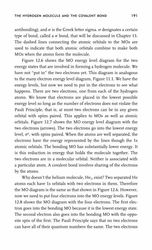
THE HYDROGEN MOLECULE AND THE COVALENT BOND 191
antibonding), and � is the Greek letter sigma. � designates a certain
type of bond, called a � bond, that will be discussed in Chapter 13.
The dashed lines connecting the atomic orbitals to the MOs are
used to indicate that both atomic orbitals combine to make both
MOs when the atoms form the molecule.
Figure 12.6 shows the MO energy level diagram for the two
energy states that are involved in forming a hydrogen molecule. Wehave not ‘‘put in’’ the two electrons yet. This diagram is analogous
to the many electron energy level diagram, Figure 11.1. We have the
energy levels, but now we need to put in the electrons to see what
happens. There are two electrons, one from each of the hydrogen
atoms. We know that electrons are placed in the lowest possible
energy level so long as the number of electrons does not violate the
Pauli Principle, that is, at most two electrons can be in any givenorbital with spins paired. This applies to MOs as well as atomic
orbitals. Figure 12.7 shows the MO energy level diagram with the
two electrons (arrows). The two electrons go into the lowest energy
level, �b, with spins paired. When the atoms are well separated, the
electrons have the energy represented by the lines though the 1s
atomic orbitals. The bonding MO has substantially lower energy. It
is this reduction in energy that holds the molecule together. Thetwo electrons are in a molecular orbital. Neither is associated with
a particular atom. A covalent bond involves sharing of the electrons
by the atoms.
Why doesn’t the helium molecule, He2, exist? Two separated He
atoms each have 1s orbitals with two electrons in them. Therefore
the MO diagram is the same as that shown in Figure 12.6. However,
now we need to put four electrons into the MO energy levels. Figure12.8 shows the MO diagram with the four electrons. The first elec-
tron goes into the bonding MO because it is the lowest energy state.
The second electron also goes into the bonding MO with the oppo-
site spin of the first. The Pauli Principle says that no two electrons
can have all of their quantum numbers the same. The two electrons

192 ABSOLUTELY SMALL
FIGURE 12.7. The MO diagram for the hydrogen molecule. The two elec-
trons (arrows), one from each hydrogen atom, go into the lowest energy
level with their spins paired. The energy is lower than the separated
atoms. An electron pair sharing bond is formed.
atomicorbital
atomicorbital
1s 1s
bonding MO b
antibonding MO *
in the bonding MO have different spin quantum numbers, s �
�1/2 and s � �1/2. There are only these two spin quantum num-
bers, so the third electron cannot go into the bonding MO. It must
go into the next lowest energy level, which is the antibonding MO.
The fourth electron can also go into the antibonding MO with the
opposite spin. There are two electrons in the bonding MO and two
electrons in the antibonding MO. The two electrons in the bonding
MO lower the energy relative to the separated atoms, but the two
electrons in the antibonding MO raise the energy just as much as
the bonding electrons lowered the energy. The net result is that
there is no decease in energy relative to the separated atoms. A
molecule is held together because the bonded atoms have lower
energy than the separated atoms. For helium atoms, there is no
reduction in energy that would produce a stable configuration.

THE HYDROGEN MOLECULE AND THE COVALENT BOND 193
FIGURE 12.8. The MO diagram for the hypothetical helium molecule.
There are four electrons (arrows), two from each helium atom. Two go
into the bonding MO. Because of the Pauli Principle, the other two go
into the antibonding MO. There is no net reduction in energy and, there-
fore, no bond.
atomicorbital
atomicorbital
1s 1s
b
*
Therefore, there is no bond. We will see this same type of behavior
for the noble gas neon in the next chapter.
To see the predictive capabilities of the simple diagrams like
those shown in Figures 12.7 and 12.8, consider four molecules, orpossible molecules. They are the hydrogen molecule ion H�
2, the
hydrogen molecule H2, the helium molecule ion He�2 , and the he-
lium molecule He2. H�2 is composed of two hydrogen nuclei (pro-
tons) and one electron. Like the atomic cation ion Na�, it is
positively charged because it has one fewer electrons than it has
protons. He�2 is the molecular ion composed of two helium nuclei
with two protons in each nucleus and three electrons. So it hasfour positive charges (four protons) and three negatively charged
electrons.
Figure 12.9 shows the MO energy level diagrams for the four
molecules. The atomic energy levels have been omitted. H�2 has
only one electron, so it goes into the lowest energy level, the bond-

194 ABSOLUTELY SMALL
FIGURE 12.9. The MO energy level diagrams for four molecules, the hy-
drogen molecule ion H�2 , the hydrogen molecule H2, the helium molecule
ion He�2 , and the helium molecule He2.
b
*
b
*
b
*
b
*
1/2 bond 1 bond 1/2 bond zero bonds
ing MO. The energy is lower than the separated atoms, but by only
approximately half as much as for the H2 molecule, which has two
electrons in the bonding MO. H2 has a full covalent bond. We say it
has a bond order of 1. He�2 has a bond order of 1/2. He�
2 has three
electrons. The first two can go into the bonding MO, but, because
of the Pauli Principle, the third electron must go into the antibond-
ing MO. Two electrons lower the energy relative to the separated
atoms, but one electron raises the energy. There is a net lowering
of the energy. The He�2 molecular ion exists in nature, and it has a
bond order of 1/2. As discussed, He2 has two bonding electrons and
two antibonding electrons. It has no bond. The bond order is zero.
The He2 molecule does not exist.
Table 12.1 gives some quantitative information about these four
molecules. It gives the number of bonding electrons, the number of
antibonding electrons, and the net, which is the number of bonding
electrons minus the number of antibonding electrons. It also gives
the bond order. The last two columns are of particular interest.
These are the results of experimental measurements on the
molecules. First consider the bond length. The lengths are in A
(Angstroms, 10�10 m). The H�2 molecule has a bond order of 1/2
and a bond length of 1.06 A. In contrast, H2, which has a full bond
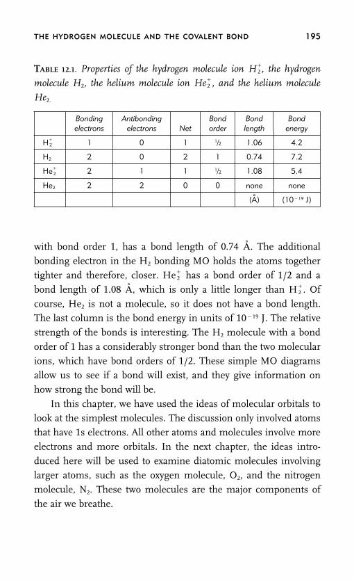
THE HYDROGEN MOLECULE AND THE COVALENT BOND 195
TABLE 12.1. Properties of the hydrogen molecule ion H�2 , the hydrogen
molecule H2, the helium molecule ion He�2 , and the helium molecule
He2.
Bonding Antibonding Bond Bond Bondelectrons electrons Net order length energy
H�2 1 0 1 1/2 1.06 4.2
H2 2 0 2 1 0.74 7.2
He�2 2 1 1 1/2 1.08 5.4
He2 2 2 0 0 none none
(A) (10�19 J)
with bond order 1, has a bond length of 0.74 A. The additional
bonding electron in the H2 bonding MO holds the atoms together
tighter and therefore, closer. He�2 has a bond order of 1/2 and a
bond length of 1.08 A, which is only a little longer than H�2 . Of
course, He2 is not a molecule, so it does not have a bond length.The last column is the bond energy in units of 10�19 J. The relative
strength of the bonds is interesting. The H2 molecule with a bond
order of 1 has a considerably stronger bond than the two molecular
ions, which have bond orders of 1/2. These simple MO diagrams
allow us to see if a bond will exist, and they give information on
how strong the bond will be.
In this chapter, we have used the ideas of molecular orbitals tolook at the simplest molecules. The discussion only involved atoms
that have 1s electrons. All other atoms and molecules involve more
electrons and more orbitals. In the next chapter, the ideas intro-
duced here will be used to examine diatomic molecules involving
larger atoms, such as the oxygen molecule, O2, and the nitrogen
molecule, N2. These two molecules are the major components of
the air we breathe.

13
What Holds
Atoms Together:
Diatomic Molecules
THE HYDROGEN MOLECULE is a diatomic molecule, that is, a molecule
composed of only two atoms. Our investigation of hydrogen revealed
how atoms can combine their atomic orbitals to form molecular orbit-
als. We need to extend our discussion of molecular orbitals to learn
how more complicated molecules are built up from atoms. First, we
will consider other diatomic molecules, for example, N2, O2, F2, andHF. N2, O2, and F2 (nitrogen, oxygen, and fluorine) are called homo-
nuclear diatomics because the two atoms are the same. HF (hydrogen
fluoride) is a heteronuclear diatomic because the two atoms are differ-
ent. Examination of homonuclear diatomics will let us go beyond the
hydrogen molecule, which is a special case. The nature of molecular
orbitals for heteronuclear diatomics is an important step toward the
study of polyatomic molecules that compose most of the molecularsubstances that surround us, from alcohol to fats.
The hydrogen molecule is the only neutral molecule that only
uses electrons in its 1s orbitals to form a chemical bond. The elec-
trons that an atom employs in bonding are called the valence elec-
trons. In the molecules N2, O2, F2, and HF, 2s and 2p orbitals are
196

WHAT HOLDS ATOMS TOGETHER: DIATOMIC MOLECULES 197
involved in bonding. The 2s and 2p electrons are the valence elec-
trons. N, O, and F are in the second row of the Periodic Table.
Atoms in the third row of the Periodic Table, such as P, S, and
Cl (phosphorus, sulfur, and chlorine), will have 3s and 3p valence
electrons involved in bonding. Atoms in the third and higher rows
of the Periodic Table can also employ d electrons in forming chemi-
cal bonds. Here we will focus on the second row elements. Thesecond row elements are of great importance, and the ideas that will
be developed are sufficiently general to cover the nature of chemical
bonding of heavier elements.
SIGMA (�) AND PI (�) BONDS
As shown in Figure 12.2, when two hydrogen atoms form the H2
molecule, the two hydrogen 1s orbitals combine to form the bond-
ing molecular orbital. There is electron density along the line that
connects the nuclei. A � (sigma) bonding or antibonding molecular
orbital has electron density along the line connecting the nuclei. In
H2, we say that a � bond is formed using a � bonding MO. s orbitals
always form � bonds. There is no way to bring together two s orbit-
als and not have electron density along the line connecting the nu-clei. This is not true for p orbitals.
Because of their shapes, there are two ways for a pair of p orbit-
als to come together, as is illustrated in Figure 13.1. The drawings
in Figure 13.1 show the p orbitals very schematically. These are
actually probability amplitude waves that have a diffuse probability
distribution of finding the electron some distance from the nucleus.
Here the outline gives a representation of the general shape of a porbital. Better illustrations are shown in Figure 10.7. Recall that a p
orbital has a nodal plane between the two lobes. A nodal plane is a
plane in which the probability of finding the electron is zero. For a
pz orbital, the nodal plane is the xy plane (see Figure 10.7). The
probability of finding an electron in some region of space is fre-

198 ABSOLUTELY SMALL
FIGURE 13.1. A pair of p orbitals brought close to each other. Upper
portion: the orbitals are brought together end to end. There is electron
density along the line connecting the nuclei. Bottom portion: the orbitals
are brought together side to side. There is no electron density along the
line connecting the nuclei.
Lobes of p orbitals point at each other.
Electron density along line connecting nucleus.
– + –+
Lobes of p orbitals are side to side.
++
––
No electron density along line connecting nuclei. Nodal plane contains nuclei.
quently called the electron density. A high density means there is a
high probability of finding the electron.
The upper portion of Figure 13.1 shows two p orbitals brought
close to each other end to end. The lobes are pointing at each other.The nuclei are represented by the dots. The dashed line is the line
connecting the nuclei. There is clearly electron density along the
line connecting the two nuclei. The lower portion of the figure
shows the two p orbitals brought close to each other side to side.
The nodal plane is perpendicular to the plane of the page. The nu-

WHAT HOLDS ATOMS TOGETHER: DIATOMIC MOLECULES 199
clei lie in the nodal plane. There is no electron density along the
line connecting the nuclei. The lobes of the p orbitals have signs.
One lobe is positive and the other negative. In Figure 13.1, the posi-
tive lobes were brought together next to each other in both the top
and bottom portions of the figure.
SIGMA MOLECULAR ORBITALS
When the orbitals are brought sufficiently close together, they can
form bonding and antibonding molecular orbits. First we will look
at molecular orbitals formed from s and p atomic orbitals that give
� bonding and antibonding MOs. A � MO has electron density
along the line joining the nuclei. As discussed above, s orbitals can
only form � orbitals because of their spherical shape. p orbitals canalso form � MOs. Figure 13.2 shows � bonding and antibonding
MOs formed from both s and p orbitals. The upper part of the figure
depicts the two possible ways that a pair of s orbitals can be com-
bined. The s orbitals are waves and can have either a � or � sign
associated with them. In the top portion, both s orbitals have �
signs. When they combine, the s orbital waves constructively inter-
fere to produce a � bonding MO. In the second line of the figure,one s orbital is � and the other is �. When they combine, they
destructively interfere to form an antibonding MO. The bonding
MO concentrates the electron density between the nuclei, while the
antibonding MO pushes the electron density to the outside, reduc-
ing the negative electron density between the nuclei. The positively
charged nuclei repel each other more strongly, making this config-
uration antibonding.The bottom portion of Figure 13.2 shows the results of combin-
ing two p orbitals to form � molecular orbitals. The � p bonding
MO is generated by overlapping the � lobe of one p orbital with
the � lobe of the other p orbital. There is constructive interference
between the � lobes, resulting in high electron density between the

200 ABSOLUTELY SMALL
FIGURE 13.2. Upper portion: a pair of s orbitals are overlapped in two
ways to give � bonding (constructive interference) and � antibonding
(destructive interference) molecular orbitals. Lower portion: a pair of p
orbitals are overlapped in two ways to give � bonding (constructive inter-
ference) and � antibonding (destructive interference) molecular orbitals.
In all cases, there is electron density along the line through the nuclei.
- s orbitals bonding
antibonding
+ + +
– + –+
+– –
- p orbitals bonding
– + –+
antibonding
– + – + – +–+
atomic nuclei. There are two nodal planes that are perpendicular tothe page. These are the two nodal planes that came from the twoatomic p orbitals. In contrast, in the bottom line of the figure, thepositive lobe of one p orbital is overlapped with the negative lobe ofthe other p orbital. The result is destructive interference, producingthe antibonding MO. The electron density is pushed to the outside,and it is greatly reduced between the two nuclei. In addition to thetwo nodal planes that come from the atomic orbitals, there is a third

WHAT HOLDS ATOMS TOGETHER: DIATOMIC MOLECULES 201
nodal plane that arises because there is complete destructive inter-ference between the positive and negative lobes of the two atomic porbitals. In these bonding and antibonding MOs formed fromatomic p orbitals, there is electron density along the line connectingthe nuclei. Therefore, these are � MOs.
PI MOLECULAR ORBITALS
s orbitals can only form � MOs, but p orbitals can form � MOs andanother type of molecular orbital called � (the Greek letter pi) MOs.When p atomic orbitals come together end to end, they form �
MOs. When they come together side to side, they form � MOs, asshown in Figure 13.3. The upper portion of the figure shows two porbitals forming a bonding molecular orbital. The positive lobe ofone atomic orbital overlaps the positive lobe of the other, and thenegative lobes overlap. There is constructive interference for boththe positive and negative lobes. As can be seen in the figure, thereis a great deal of electron density in the area between the two nuclei.However, there is no electron density directly along the line con-necting the nuclei. There is a nodal plane that is perpendicular tothe plane of the page because each atomic orbital has a nodal planeperpendicular to the page. The nodal plane contains the nuclei. Inspite of the nodal plane, all of that electron density immediatelyabove and below the line connecting the nuclei reduces the repul-sion of the positive nuclear changes. The energy is lower than theseparated atoms resulting in a � bonding MO.
The lower portion of Figure 13.3 shows the � antibonding MO.The two p atomic orbitals come together side to side, but the posi-tive lobe of one orbital overlaps the negative lobe of the other orbital,and vice versa. The result is destructive interference between thelobes giving rise to the � antibonding MO. The antibonding MOhas much less electron density between the nuclei. The result isthat the energy is higher than the separated atoms, so this config-uration of atomic orbitals produces an antibonding MO.

202 ABSOLUTELY SMALL
FIGURE 13.3. Upper potion: a pair of p orbitals are overlapped side to
side to give a � bonding molecular orbital (constructive interference).
There is no electron density along the line connecting the nuclei. Lower
portion: a pair of p orbitals are overlapped side to side to give a � anti-
bonding molecular orbital (destructive interference). Note the signs of the
lobes of the p atomic orbitals. The antibonding MO has a node between
the nuclei.
- p orbitals bonding
+
–
+
–
+
–
Node along internuclear axis, but not between nuclei.
antibonding
Node between nuclei.
Node along internuclear axis.
+
+
–
–
+
–+
–
�
BONDING IN DIATOMIC MOLECULES:THE FLUORINE MOLECULE
We are now ready to discuss bonding for diatomics with atoms
other than hydrogen. Let’s start with the diatomic, F2, the fluorine
molecule. We will use the same approach as we did for H2, but now

WHAT HOLDS ATOMS TOGETHER: DIATOMIC MOLECULES 203
there are more orbitals and more electrons involved. We imagine
bringing two F atoms together and stopping at the point where the
energy is lowest. This is the separation of the two F atoms when
they are bonded (assuming they form a bond), as in Figure 12.5. We
can draw an energy level diagram, as in Figure 12.6. We need to
define the axis along which the two atoms approach each other be-
cause we have pz, px, and py orbitals. It matters whether we bring porbitals together end to end or side to side. When the two atoms
(labeled a and b) approach along the z axis (see Figure 13.4), the pz
orbitals will come together end to end, while the px and py orbitalswill come together side to side. Therefore, the pz atomic orbitals willform � MOs and the px and py atomic orbitals will form � MOs.
Figure 13.5 shows the energy level diagram for two F atomsbrought together along the z axis. In the diagram, the energy levelsfor the atomic orbitals for the two atoms (a and b) are shown on theright and left sides of the diagram. The corresponding bonding (b)and antibonding (*) MOs are shown in the center. � MOs formedfrom s atomic orbitals have a subscript s. � MOs formed from pz
atomic orbitals have a subscript z, and � MOs formed from px or py
atomic orbitals have a subscript x or y. The bonding MO is alwayslower in energy than the atomic orbitals that formed it, and theantibonding MO is always higher in energy. The three p atomicorbitals have the same energy. When quantum states have the sameenergy, they are said to be degenerate. In the diagram, the three patomic orbitals are shown as three closely spaced lines even thoughthey are degenerate. As shown, only the matching atomic orbitals
FIGURE 13.4. Two atoms are brought together along the z axis. Pz orbit-
als will approach end to end; px and py orbitals will approach side to side.
Za b

204 ABSOLUTELY SMALL
FIGURE 13.5. The energy level diagram for two fluorine atoms, a and b,
brought together to form molecular orbitals. The atomic orbital energies
are on the right and left sides. The bonding (b) and antibonding (*) MO
energy levels are in the center. There are � and � MOs. The three atomic
p orbitals have the same energies. These are shown as three closely spaced
lines. The spacings between the levels are not to scale.
1sa
2sa
1sb
2sb
2px,y,z,a 2px,y,z,b
�
� �
�
of the same energy combine to make MOs. Quantum theory gives
this result. States of identical energy can readily combine to make
superposition states. In this case, atomic orbitals of identical energy
on two different atoms can combine to make molecular orbitals. In
general, only atomic states with similar energy can combine to
make MOs. This will be important when we discuss heteronuclear
diatomics below. For the homonuclear diatomics, the atomic orbit-
als are identical in energy. In the diagram, the three p orbitals on

WHAT HOLDS ATOMS TOGETHER: DIATOMIC MOLECULES 205
each atom, a total of six atomic orbitals, combine to form six molec-
ular orbitals. The pz atomic orbitals produce the � bonding and
antibonding MOs, which are different in energy from the bonding
and antibonding �x and �y MOs formed from the px and py atomic
orbitals. However, the �x and �y bonding MOs have the same en-
ergy, and the �x and �y antibonding MOs have the same energy.
The degenerate pairs of � MOs are shown as two closely spacedlines.
Fluorine has nine electrons. So a fluorine atom will have two
electrons in the 1s orbital, two electrons in the 2s orbital, and five
electrons in the three 2p orbitals. Two F atoms have a total of 18
electrons. We now need to place the 18 electrons in the proper molec-
ular orbitals in a manner equivalent to the way we placed the elec-
trons in the atomic orbitals when we were building up the PeriodicTable in Chapter 11 and the hydrogen molecule in Chapter 12. As
before, we need to follow the three rules for filling the MOs. First is
the Pauli Principle, which states that at most two electrons can be in
an orbital and the two must have opposite spins. Opposite spins are
represented by one up arrow and one down arrow. Second, electrons
are placed in the lowest energy level first, consistent with the Pauli
Principle. Third is Hund’s Rule, which states that electrons will notpair their spins if possible. In F2, Hund’s Rule will not change the
results of placing the electrons in the proper orbitals. When we con-
sider oxygen, O2, it will be important.
Figure 13.6 is the MO energy level diagram for F2 with the elec-
trons placed in the proper orbitals. The atomic orbital energy levels
shown in Figure 13.5 are not included. Only the MO energy levels
are shown. The first two electrons go into the � bonding MO formedfrom 1s orbitals. The next two electrons go in the � antibonding MO
formed from 1s orbitals. The electrons in the bonding MO are lower
in energy than the atomic orbitals of the separated atoms, but the
electrons in the antibonding MO are the same amount higher in
energy. Therefore, these four electrons do not contribute to bonding

206 ABSOLUTELY SMALL
FIGURE 13.6. The molecular orbital energy level diagram for the F2, flu-
orine diatomic molecule. The atomic orbital energies are not shown. Two
fluorine atoms have 18 electrons. These have been placed in the orbitals
following the rules discussed for atomic orbitals in Chapter 11. There is
one more filled bonding MO than antibonding MO. F2 has a single bond.
From 1s atomicorbitals
From 2s atomicorbitals
From 2p atomicorbitals
� �
� �
in F2. The next four electrons go in the � bonding and antibondingMOs formed from the 2s atomic orbitals. Again, these do not contrib-
ute to bonding because there are two electrons in the bonding MO
and two electrons in the antibonding MO.
Now the p electrons come into play. There are a total of 10, five
from each F atom. The first two go into the � bonding MO formed
from the pz atomic orbitals. Then four electrons go into the �x and

WHAT HOLDS ATOMS TOGETHER: DIATOMIC MOLECULES 207
�y bonding MOs. Four electrons can go into these � molecular or-
bitals because there are two MOs, and each can take two electrons
according to the Pauli Principle. The last four electrons go into the
�x and �y antibonding MOs. The four electrons in the � antibond-
ing MOs cancel the bonding effect of the four electrons in the �
bonding MOs. Therefore, the � electrons do not contribute to bond-
ing. However, nothing cancels the two electrons in the � bondingMO formed from the pz atomic orbitals because there are no elec-
trons in the corresponding antibonding MO. The net result is that
one pair of bonding electrons is not canceled out, so F2 has a bond
order of 1 like H2. We say that F2 has a single bond, and it is a �
bond. The single covalent bond comes from having two electrons
in a bonding MO. Molecular orbitals are probability amplitude
waves that span the entire molecule. The atomic nuclei share theseelectrons.
THE NEON MOLECULE DOESN’T EXIST
We can use the same MO energy level diagram shown in Figure
13.6 to consider the hypothetical diatomic neon molecule, Ne2.
Neon is immediately to the right of fluorine on the Periodic Table.Figure 13.7 shows the results of placing the 20 electrons from two
neon atoms into the MO energy level diagram. The first 18 electrons
go in the same as in F2. However, there are two more electrons, and
they must go in the �*z antibonding MO. Therefore, for every pair of
electrons in a bonding MO there is a pair of electrons in an anti-
bonding MO. The result is no bonding. The molecule Ne2 does not
exist. Other noble gas homonuclear diatomics do not exist. The ex-ample of Ne2 indicates why. A noble gas atom has a closed shell.
Two noble gas atoms have just the right number of electrons to fill
all of the bonding and antibonding MOs. Therefore, no net bonds
are formed.
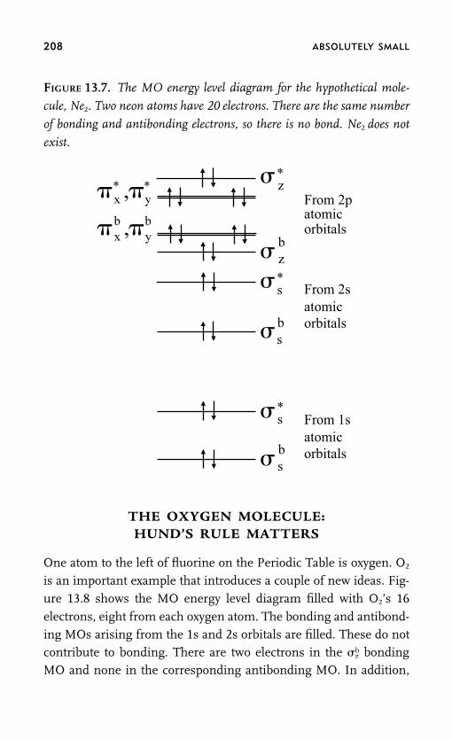
208 ABSOLUTELY SMALL
FIGURE 13.7. The MO energy level diagram for the hypothetical mole-
cule, Ne2. Two neon atoms have 20 electrons. There are the same number
of bonding and antibonding electrons, so there is no bond. Ne2 does not
exist.
From 1s atomicorbitals
From 2s atomicorbitals
From 2p atomicorbitals
� �
� �
THE OXYGEN MOLECULE:HUND’S RULE MATTERS
One atom to the left of fluorine on the Periodic Table is oxygen. O2
is an important example that introduces a couple of new ideas. Fig-ure 13.8 shows the MO energy level diagram filled with O2’s 16electrons, eight from each oxygen atom. The bonding and antibond-ing MOs arising from the 1s and 2s orbitals are filled. These do notcontribute to bonding. There are two electrons in the �b
z bondingMO and none in the corresponding antibonding MO. In addition,

WHAT HOLDS ATOMS TOGETHER: DIATOMIC MOLECULES 209
FIGURE 13.8. The MO energy level diagram for oxygen, O2. There is one
extra pair of � bonding electrons and one extra pair of � bonding elec-
trons. O2 has a double bond. Note the unpaired electrons in the � anti-
bonding MOs.
From 1s atomicorbitals
From 2s atomicorbitals
From 2p atomicorbitals
� �
� �
there are four electrons in the two � bonding MOs but only two
electrons in the � antibonding MOs. The result is one � bond andone � bond. Oxygen has a bond order of 2. It has a double bond. As
will be discussed further below, a double bond is stronger and
shorter than a single bond.
O2 is the first example where Hund’s Rule comes into play and
is important. Note that in filling the energy levels with electrons,
the last two electrons have their spins unpaired. It is possible to
have unpaired spins without violating the Pauli Principle because

210 ABSOLUTELY SMALL
there are two distinct � antibonding MOs. �*x comes from the side-
to-side overlap of the two px atomic orbitals (see Figure 13.3), and
�*y, comes from the side-to-side overlap of the two py atomic orbitals.
Hund’s Rule says that the electrons will go into orbitals unpaired if
the result doesn’t violate the Pauli Principle and doesn’t require
using a much higher energy orbital. The two � antibonding MOs
have identical energy, so Hund’s Rule comes into play.An electron has a magnetic moment. In some sense it acts like
a tiny bar magnet. It has a north pole and a south pole. The term
spin for the electron quantum number comes from classical me-
chanics. In classical mechanics, a charge distribution that is spin-
ning has a magnetic moment. An electron is a probability
amplitude wave. It has a delocalized charge distribution. It has a
magnetic moment, but it is not literally spinning. That is a classicalidea. Dirac, who gave us the concept of absolute size (see Chapter
2), also showed why an electron has a magnetic moment by combin-
ing quantum theory and Einstein’s Theory of Relativity. Although
an electron is not actually spinning, the name stuck, and the mag-
netic moment of the electron is important.
When two electron spins are paired, the north pole of one little
magnet is matched with the south pole of the other. The magneticproperty of one electron cancels the magnetic property of the other.
However, in O2, two of the electrons are not paired. Their spins
point in the same direction. The result is that the O2 molecule is
referred to as being paramagnetic. It will respond to a magnet. O2
is a gas at room temperature, but if you make it very cold, below
�183� C (�297� F) it will become a liquid. Water above 100� C is a
gas, but if you cool it below 100� C, it becomes a liquid. O2 is thesame, but you need to make it much colder. It is possible to put
liquid O2 in a test tube hanging from a string. If you bring a magnet
up to the test tube, you can actually pull the test tube around with
the magnet. The electron spins (little bar magnets) of O2 are lined
up by the magnetic field of the external macroscopic magnet. These

WHAT HOLDS ATOMS TOGETHER: DIATOMIC MOLECULES 211
lined-up little bar magnets add together to make the liquid O2 mag-
netic, and the test tube of O2 is attracted to the external magnet. The
correct prediction that O2 is paramagnetic from the analysis we have
done using the MO energy level diagram is remarkable. The mag-
netic moment of O2 is strictly a quantum effect, and our prediction
that O2 is paramagnetic comes from the application of Hund’s Rule.
By following some rules, we drew some lines to represent the en-ergy levels. Then following more rules, we put some arrows up and
down on the energy level lines (we put in the electrons). Using these
lines and arrows we can say that the oxygen molecule is magnetic
while the fluorine and nitrogen molecules are not.
THE NITROGEN MOLECULE
Figure 13.9 shows the filled MO energy level diagram for nitrogen,
N2. The nitrogen atom is immediately to the left of oxygen on the
Periodic Table. Note that there is a switch in the ordering of the
bonding MOs derived from the p electrons. Detailed quantum me-
chanical calculations give the ordering and the actual energies of
the MO energy levels. For nitrogen, the ordering is different than
for O2 and F2. The nitrogen atom has seven electrons, so N2 has atotal of 14 electrons. As with F2 and O2, the 1s and 2s electrons do
not play a role in bonding because they fill both the bonding and
antibonding MOs. Filling these MOs uses up eight of the 14 elec-
trons. The other six electrons fill the three bonding MOs, one � MO
and two � MOs. There are no electrons in the � antibonding MOs
or the � antibonding MO formed from the pz orbitals. Therefore,
N2 has a bond order of 3, a triple bond. A triple bond will be strongerand shorter than a double or single bond. Note that there are no
unpaired electrons in N2. N2 is not paramagnetic. At low tempera-
ture, below �196� C (�320� F), N2 is a liquid. However, you cannot
move a test tube of liquid N2 with a magnet because it does not have
unpaired spins.

212 ABSOLUTELY SMALL
SINGLE, DOUBLE, AND TRIPLE BONDS
In discussing bonding in Chapter 11 based on an atom’s position
in the Periodic Table, we used the idea that an atom would form
covalent bonds to share electrons so that it could reach the noble
gas configuration. For the second row elements we have been dis-
cussing here, nitrogen, oxygen, and fluorine, the noble gas is neon.
We said that F, which is one electron from the Ne configuration,
would share one electron with another atom. O, which is two elec-
trons from the Ne configuration, would share two electrons, and N,
which is three electrons from Ne, would share three electrons. Here
we saw that F2 has a single bond, O2 has a double bond, and N2 has
a triple bond. The type of bond between atoms, that is single, dou-
ble, or triple, can be indicated as F�F, O�O, and N�N. It is
through the bonds that atoms share electrons. A covalent bond is
an electron pair sharing bond. A double bond shares two pairs of
electrons. A triple bond shares three pairs of electrons. When a
bonding MO is exactly canceled by its corresponding antibonding
MO, the electrons are not really shared by the atoms. They are in
molecular orbitals, but the bonding MO produces constructive in-
terference of the probability amplitude waves and the antibonding
MO generates destructive interference. These cancel each other.
The electrons in this situation are referred to as lone pairs. These
are pairs of electrons that do not contribute to bonding. It is the F2
single bond, a shared pair of electrons, that provides the extra elec-
tron each F atom needs to give it the Ne configuration. In O2, the
double bond (sharing of two pairs of electrons) provides two extra
electrons for each O atom to give them the Ne configuration. In N2,
the triple bond (sharing of three pairs of electrons) provides three
extra electrons for each nitrogen atom to give them the Ne configu-
ration.
In the series F2, O2, and N2, we have a single bond, double bond,
and triple bond. The electron sharing gives each atom the Ne con-

WHAT HOLDS ATOMS TOGETHER: DIATOMIC MOLECULES 213
figuration. The next element to the left of nitrogen in the Periodic
Table is carbon. One might assume that carbon would make a qua-
druple bond to form C2 and get to the Ne configurations. C2 doesn’t
exist as a stable molecule. You can see why by looking at Figure
13.9, the MO diagram for N2, and removing the two electrons with
the highest energy, the �bz bonding MO. This would be the C2 elec-
tron configuration. However, it would have a double bond from thefour electrons in the two � bonding MOs, not a quadruple bond.
These two bonds would mean that the carbons in C2 would only
have gained two extra electrons through sharing, not the four extra
FIGURE 13.9. The MO energy level diagram for nitrogen, N2. There is
one extra pair of � bonding electrons and two extra pairs of p bonding
electrons. N2 has a triple bond.
From 1s atomicorbitals
From 2s atomicorbitals
From 2p atomicorbitals
� �
� �

214 ABSOLUTELY SMALL
electrons each carbon needs to obtain the Ne configuration. Carbon
needs to make four bonds to obtain the Ne configuration by form-
ing molecules such as CH4. It can’t make four bonds by forming
the C2 molecule, and C2 doesn’t exist.
F2 has a single bond, O2 has a double bond, and N2 has a triple
bond. Table 13.1 illustrates how the bond order strongly affects the
properties of the bond. As the bond order increases, the bond lengthgets shorter and the bond energy increases. The bond energy is the
energy that needs to be put into the molecule to break the bond.
Breaking the bond means separating the atoms to a distance so far
apart that they no longer feel each other. As will be discussed in the
next chapter, carbon can make single, double, and triple bonds to
another carbon atom while at the same time forming bonds to other
atoms, such has hydrogen. Before we can discuss molecules that arelarger than diatomics, we need to go beyond homonuclear diatomic
molecules and examine heteronuclear diatomics to see how molecu-
lar orbitals are formed from nonidentical atoms.
HETERONUCLEAR DIATOMICS
In homonuclear diatomics, the MOs are formed from atomic orbit-
als with identical energies. In a heteronuclear diatomic, for example
hydrogen fluoride (HF), the two atoms are different. Because the
atoms are different, the atomic orbitals’ energies of one atom will
TABLE 13.1. The Effect of Bond Order on Bond Properties.
F2 O2 N2
bond order single (1) double (2) triple (3)
bond length (A) 1.42 1.21 1.10
bond energy (10�19 J) 2.6 8.3 15.6

WHAT HOLDS ATOMS TOGETHER: DIATOMIC MOLECULES 215
not match those of the other. For HF, the hydrogen atom has a
single electron in the 1s orbital. F has nine electrons in the 1s, 2s,
and 2p orbitals. Both F2 and H2 have single bonds. Looking at Fig-
ure 13.6, the single bond in F2 is a � bond due to the bonding MO,
�bz . This bonding MO was formed from two 2pz atomic orbitals,
one on each F atom. H2 has a single � bond due to the bonding MO
formed from two 1s orbitals (see Figure 12.7). To make HF, thequestion is, which orbital on F will combine with the 1s orbital on
H to give MOs involved in bonding? Quantum theory calculations
show that states (atomic orbitals) that are close in energy can com-
bine to produce electron sharing MOs. Atomic orbitals with signifi-
cantly different energies form MOs that are essentially equal to the
individual atomic orbitals, and they do not contribute to bonding.
The hydrogen 1s orbital has an energy of �2.2 � 10�18 J. (Re-call that the negative sign means that the electron is bound.) The
energy of the fluorine 1s orbital (measured in the F2 molecule) is
�1.1 � 10�16 J. So the 1s orbital of F is about 50 times lower in
energy than the 1s orbital of H. This is a tremendous difference in
energy, and the H 1s will not form a MO with the F 1s. In contrast,
an F 2p orbital has an energy of �2.8 � 10�18 J. This energy is
about 25% below the H 1s energy, which is close in energy. So anF 2p and the H 1s orbital energies are similar enough that they will
form true MOs.
There are three F 2p orbitals, 2pz, 2px, and 2py. To decide which
of these will interact with the H 1s, we need to define how we bring
the atoms together. Let’s say we bring the H atom and the F atom
toward each other along the z axis as shown at the top of Figure
13.10. The two circles reflect the correct relative sizes of the H andF atoms. Fluorine’s 2py orbital has its lobes perpendicular to the z
axis, as shown in the middle portion of the figure. (The orbitals are
not drawn to scale.) When the 2py overlaps the hydrogen 1s orbital,
the positive 2py lobe will constructively interfere with the 1s orbital,
but the negative lobe will destructively interfere. The net result is

216 ABSOLUTELY SMALL
FIGURE 13.10. Top: H and F atoms brought together along the z axis.
Circles show the relative size of the atoms. Middle: overlap of the H 1s
and F 2py orbitals. There is equal constructive (�) and destructive (�)
interference in the overlap region. No MO formation. Bottom: overlap of
the H 1s and the F 2pz orbitals. There is constructive interference in the
overlap region.
H1s
+ + –
F2pz
+
H F z
H1s
+ +
–F2py
+
–z
z
that there is no net constructive or destructive interference. Thesame is true for the 2px orbital. The 2py and 2px orbitals will notform bonding or antibonding MOs in the HF molecule. The lowerportion of the figure shows the 2pz orbital’s positive lobe overlap-ping with the 1s orbital, which is also taken to be positive. Thisoverlap will result in constructive interference of the probability am-plitude waves, and can produce a bonding MO. Since there is elec-tron density along the line connecting the nuclei, the bond will bea � bond. If the F negative 2pz lobe overlaps with the H positive1s lobe, there will be destructive interference that gives rise to anantibonding MO.
As discussed above, the fluorine 1s orbital energy is so much

WHAT HOLDS ATOMS TOGETHER: DIATOMIC MOLECULES 217
lower than the hydrogen 1s, that the fluorine 1s electrons do not
participate in bonding. The outermost electrons in an atom, that is,
the last shell that is filled, are the ones that contribute to bonding.
These are the valence electrons. For elements in the second row of
the Periodic Table, like fluorine, the 2s and 2p are the valence elec-
trons. In making molecular orbital energy level diagrams, usually
only the orbitals associated with the valence electrons are shown
because these are the orbitals that can be involved in bonding. Fig-
ure 13.11 shows the MO energy level diagram for HF with the F 1s
orbital and electrons left out. The energy level spacings are not to
scale. As discussed in connection with Figure 13.10, the H 1s
atomic orbital will combine with the F 2pz atomic orbital to form
bonding (�b) and antibonding (�*) MOs. This is indicated in the
diagram by the dashed lines. This diagram is similar to the energy
level diagram in Figure 13.5 except that now the atomic orbitals that
form the MOs do not have identical energies.
Fluorine has nine electrons. Two are in the 1s orbital, which
leaves seven. Hydrogen has one electron. So there are a total of
eight valence electrons to place in the MO energy levels. The first
two go into the level labeled 2s. The fluorine 2s orbital is much
lower in energy than the hydrogen 1s, and these electrons do not
participate in bonding. Therefore, the 2s molecular orbital is essen-
tially the same as the fluorine 2s atomic orbital. The two electrons
in the 2s orbital are a lone pair. The next two electrons go into the
�b bonding MO. The final four electrons go into the 2px and 2py
orbitals. Again, these are basically atomic orbitals of fluorine. They
do not play a role in the bonding. These four electrons comprise
two more lone pairs. While the lone pairs do not play a role in
bonding, in polyatomic molecules they influence the shapes of mol-
ecules, which will be discussed in Chapter 14. The net result is
that there are two electrons in the bonding MO and none in an
antibonding MO. Therefore, HF has a single bond. Hydrogen and
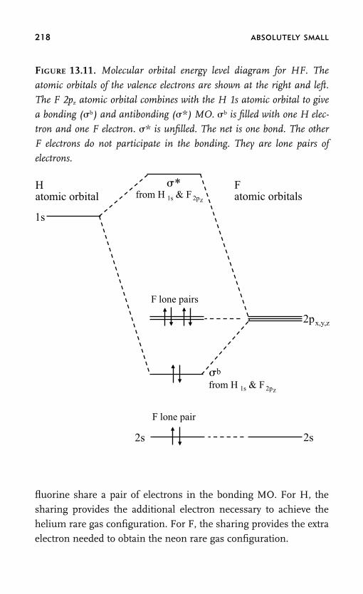
218 ABSOLUTELY SMALL
FIGURE 13.11. Molecular orbital energy level diagram for HF. The
atomic orbitals of the valence electrons are shown at the right and left.
The F 2pz atomic orbital combines with the H 1s atomic orbital to give
a bonding (�b) and antibonding (�*) MO. �b is filled with one H elec-
tron and one F electron. �* is unfilled. The net is one bond. The other
F electrons do not participate in the bonding. They are lone pairs of
electrons.
Hatomic orbital
Fatomic orbitals
2s
2s
F lone pair
F lone pairs
2px,y,z
b
*
1s
from H 1s & F 2pz
from H 1s & F 2pz
fluorine share a pair of electrons in the bonding MO. For H, the
sharing provides the additional electron necessary to achieve the
helium rare gas configuration. For F, the sharing provides the extra
electron needed to obtain the neon rare gas configuration.

WHAT HOLDS ATOMS TOGETHER: DIATOMIC MOLECULES 219
VISUAL MODELS OF MOLECULES
HF like F2, O2, and N2 are diatomics and therefore linear molecules.In the next chapter, we will talk about molecules with more complexshapes. The structure of molecules can be shown in a number ofways. HF can be written as H�F to indicate there is a single bond.In more complicated molecules, this type of representation canshow which atoms are bonded to each other and the bond order.However, it cannot display the three-dimensional geometry or givea feel for what the molecule actually looks like. Now to say a mole-cule looks like something is fundamentally incorrect. HF has twonuclei surrounded by the probability amplitude waves that are theelectrons. Nonetheless, there are representations that are useful indiscussing the nature of molecules. Figure 13.12 displays two suchrepresentations of HF. The top portion is a ball-and-stick molecularmodel. It shows the connection between the atoms and their relativesize. H is light in color and F is dark in color. The bond between
FIGURE 13.12. Representations of the HF molecule. H: light; F: dark.
Top: a ball-and-stick version that shows how the atoms are bonded and
the relative sizes of the atoms. Bottom: a space-filling version that is more
realistic.
220 ABSOLUTELY SMALL
the atoms is much too long. The bottom portion of the figure shows
a space-filling model. Most of the electron density is inside of the
overlapping spheres. The sizes and the internuclear separations are
correct. The colors and the sharp line between the atoms are to aid
the eye. There is no actual separation of the electrons between the
atoms.
The material presented in this chapter and in the next chapteris necessary to understand bonding in polyatomic molecules. In the
next chapter, we need to extend the ideas presented here to mole-
cules with more than two atoms. Polyatomic molecules have
shapes, and to understand the shapes, we will introduce new ideas,
hybrid atomic orbitals. The material developed in Chapters 13 and
14 will be used in subsequent chapters to examine a wide variety of
problems such as what are trans fats and why are they differentfrom other fats.

14
Bigger Molecules:
The Shapes of
Polyatomic Molecules
THE WORLD AROUND US is composed of polyatomic molecules. Polya-
tomic molecules are molecules with more than two atoms. These
range in size from triatomic molecules, such as carbon dioxide
(CO2), which is a major greenhouse gas, to molecules with thou-
sands of atoms, such as large proteins that are responsible for most
biological functions. As discussed in Chapter 13, diatomic mole-cules can only have one shape, linear. Larger molecules, however,
can have very complicated shapes and structures. For example, satu-
rated fats, unsaturated fats, or polyunsaturated fats differ by their
shapes and structures, which are determined by the nature of chem-
ical bonds. A given large molecule can have more than one shape.
Trans fats, which are currently being at least partially removed from
food (see Chapter 16), only differ in their shape from moleculesmade up of the same sequence of atoms that are not trans fats. A
central question in molecular matter is, how do molecules achieve
their shapes and how are different shapes possible for molecules
made of the same atoms connected together in the same way?
Before proceeding, it is worth stating that the covalent bond,
221

222 ABSOLUTELY SMALL
which is responsible for holding atoms together to form molecules,
is an intrinsically quantum mechanical phenomenon. It was not
possible to explain the nature of chemical bonds or the structure
of molecules before the advent of quantum theory. Linus Pauling
(1901–1994) won the Nobel Prize in Chemistry in 1954 ‘‘for his
research into the nature of the chemical bond and its application to
the elucidation of the structure of complex substances.’’ It is note-worthy that Linus Pauling is one of the few people to win two Nobel
Prizes. In 1962 he won the Nobel Peace Prize.
MOLECULAR SHAPES—TETRAHEDRAL METHANE
To examine the shapes of molecules and how chemical bonding cangive rise to different shapes, we need to introduce some new ideas
about atomic orbitals. We will use methane as an example of a rela-
tively simple polyatomic molecule to bring out the important issues.
Methane (natural gas) is CH4. Now, look again at carbon’s posi-
tion in the Periodic Table (Figure 11.4). Note that carbon needed to
make four electron pair sharing covalent bonds to achieve the neon
closed shell configuration. In methane, carbon makes four bondswith four hydrogen atoms. The connectivity of the atoms can be
shown in a simple diagram, which is the left portion of Figure 14.1.
Each line represents an electron pair covalent bond. However, this
diagram does not tell much about methane’s shape. Methane is not
flat. The right side of the figure shows a ball-and-stick model of the
three-dimensional shape of methane. (See the end of Chapter 13 for
a discussion of ball-and-stick and space-filling models.) Methane isa perfect tetrahedron. Imagine having a model like the right side of
Figure 14.1 and gluing a triangular piece of paper with sides of equal
length that just covered three of the hydrogen atoms. You can glue
on four such triangles, three sides and the bottom. These four trian-
gles form a perfect triangular pyramid with the hydrogens at the
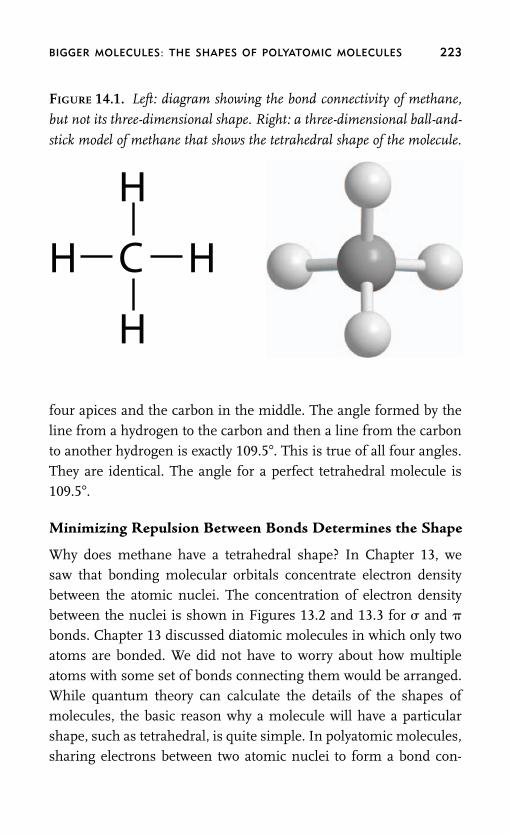
BIGGER MOLECULES: THE SHAPES OF POLYATOMIC MOLECULES 223
FIGURE 14.1. Left: diagram showing the bond connectivity of methane,
but not its three-dimensional shape. Right: a three-dimensional ball-and-
stick model of methane that shows the tetrahedral shape of the molecule.
HH
H
H
C
four apices and the carbon in the middle. The angle formed by theline from a hydrogen to the carbon and then a line from the carbonto another hydrogen is exactly 109.5�. This is true of all four angles.They are identical. The angle for a perfect tetrahedral molecule is109.5�.
Minimizing Repulsion Between Bonds Determines the Shape
Why does methane have a tetrahedral shape? In Chapter 13, wesaw that bonding molecular orbitals concentrate electron densitybetween the atomic nuclei. The concentration of electron densitybetween the nuclei is shown in Figures 13.2 and 13.3 for � and �
bonds. Chapter 13 discussed diatomic molecules in which only twoatoms are bonded. We did not have to worry about how multipleatoms with some set of bonds connecting them would be arranged.While quantum theory can calculate the details of the shapes ofmolecules, the basic reason why a molecule will have a particularshape, such as tetrahedral, is quite simple. In polyatomic molecules,sharing electrons between two atomic nuclei to form a bond con-

224 ABSOLUTELY SMALL
centrates electron density between the nuclei, just as it does with
diatomic molecules. However, in polyatomics, we have a number of
bonds, each of which has a high density of negatively charged elec-
trons. The negatively charged regions, the bonds, repel each other.
Basically, the bonds want to stay as far away from each other as
possible. These regions of high negatively charged electron density
want to overlap as little as possible. Forming bonds lowers the en-ergy of the system relative to the separated atoms. If the energy is
not lowered, bonds will not be formed. But to make the energy as
low as possible, the system of atoms assumes a configuration that
minimizes the electron repulsions by keeping the bonds away from
each other.
In methane, the tetrahedral shape minimizes the repulsions be-
tween the bonds. Look at the left-hand drawing in Figure 14.1. Thefour hydrogens are in a plane. If I keep them in the plane, they are
as well separated as possible. The angle formed by two adjacent
bonds is 90�. With the atoms in the plane, if I make one of the
angles larger than 90� to further separate two of the hydrogen-
carbon bonds, these bonds get closer to the other two bonds. So if
the four hydrogen atoms are kept in the same plane as the carbon
atom, the best that can be done is to have 90� bond angles.However, there is no reason that all of the atoms have to lie in
a plane. In the structure on the left side of Figure 14.1, the angle
between the top and bottom H atoms is 180�, and these two C-H
bonds are far apart; the same is true for the left and right H atoms.
Imagine pulling the top and bottom H atoms above the plane of the
page, while keeping the bond lengths the same and pushing the
right and left H atoms below the plane of the page. The top andbottom C-H bonds are getting closer together and the angle is re-
duced to less than 180�, but they are getting further away from the
left and right C-H bonds. Bringing the top and bottom C-H bonds
above the plane and pushing the left and right C-H bonds below
the plane reduces the overall bond-bond interaction. The interaction

BIGGER MOLECULES: THE SHAPES OF POLYATOMIC MOLECULES 225
between the top and bottom bonds is increased, but they were very
far apart to begin with. This is also true of the left and right bonds.
However, if the top-bottom and left-right angles are reduced too
much, the repulsion will go up again. There is a best angle, and
that is 109.5�, the tetrahedral angle. This is the angle that keeps the
electrons in the four C-H bonds as far apart as possible.
Lone Pairs Also Matter
In Chapter 11, we found that to obtain a closed shell configuration,
C needs to form four bonds, N needs to form three bonds, and O
needs to form two bonds. If the bonds are to hydrogens, then we
have methane, ammonia, and water, CH4, NH3, and H2O. In dis-
cussing HF at the end of Chapter 13, we noted that some of the F
electrons were not involved in bonding at all. The electrons were
paired in what are essentially atomic orbitals called lone pairs. Lone
pairs are pairs of nonbonding electrons that give rise to high elec-
tron density in the region of space they occupy. Electrons in bonds
do not want to be near electrons in lone pairs. So, although they are
not bonds, lone pairs also influence the shapes of molecules. In a
bond, the electrons are shared and more or less concentrated be-
tween two atoms. Lone pairs do not have a second atom to hang on
to. As a result, the lone pair electron distribution is bunched closer
to the atom they belong to, and it is somewhat ‘‘fatter’’ than a bond
pair distribution.
Figure 14.2 shows models of methane, ammonia, and water.
Ammonia has one lone pair, and water has two lone pairs. If you
include the lone pairs, all three molecules are basically tetrahedral
in shape. However, ammonia and water are not perfect tetrahe-
drons. The lone pair in ammonia is more spread out than the bond
pairs. To minimize the overall electron-electron repulsion to pro-
duce the lowest energy, the bonds move away from the lone pair,
thereby bringing the bonds closer together. The HNH angle in am-
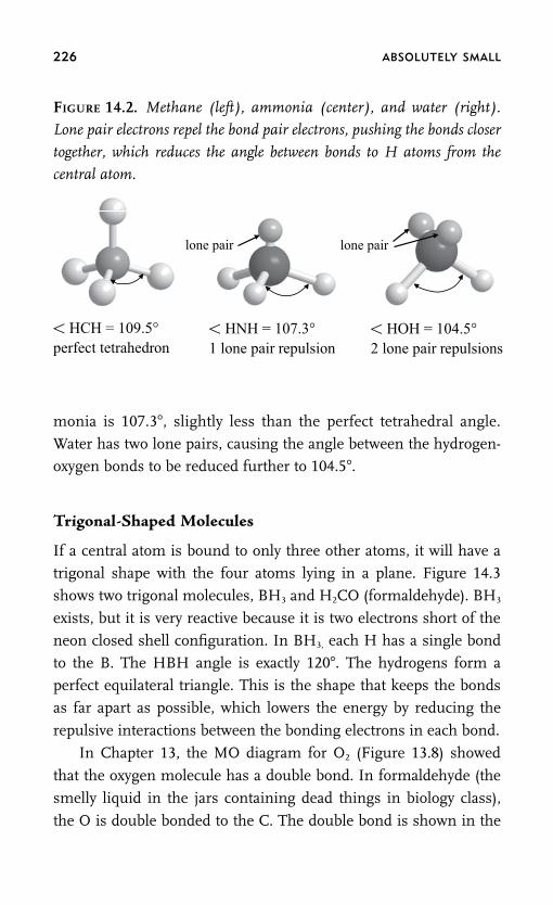
226 ABSOLUTELY SMALL
FIGURE 14.2. Methane (left), ammonia (center), and water (right).
Lone pair electrons repel the bond pair electrons, pushing the bonds closer
together, which reduces the angle between bonds to H atoms from the
central atom.
< HCH = 109.5° perfect tetrahedron
< HNH = 107.3° 1 lone pair repulsion
< HOH = 104.5° 2 lone pair repulsions
lone pair lone pair
monia is 107.3�, slightly less than the perfect tetrahedral angle.
Water has two lone pairs, causing the angle between the hydrogen-
oxygen bonds to be reduced further to 104.5�.
Trigonal-Shaped Molecules
If a central atom is bound to only three other atoms, it will have a
trigonal shape with the four atoms lying in a plane. Figure 14.3
shows two trigonal molecules, BH3 and H2CO (formaldehyde). BH3
exists, but it is very reactive because it is two electrons short of the
neon closed shell configuration. In BH3, each H has a single bond
to the B. The HBH angle is exactly 120�. The hydrogens form a
perfect equilateral triangle. This is the shape that keeps the bonds
as far apart as possible, which lowers the energy by reducing the
repulsive interactions between the bonding electrons in each bond.
In Chapter 13, the MO diagram for O2 (Figure 13.8) showed
that the oxygen molecule has a double bond. In formaldehyde (the
smelly liquid in the jars containing dead things in biology class),
the O is double bonded to the C. The double bond is shown in the

BIGGER MOLECULES: THE SHAPES OF POLYATOMIC MOLECULES 227
FIGURE 14.3. Left: BH3. The atoms lie in a plane. The HB bonds are
single, and the hydrogens form a perfect equilateral triangle. Each HBH
bond angle is 120. Right: H2CO (formaldehyde). The atoms lie in a
plane. The CO bond is a double bond. The angles are unequal.
120°
B
H
H H
122.4°
C
O
H H
115.8°
ball-and-stick figure model as two cylinders joining the atoms ratherthan one. The double bond gives the O the neon closed shell con-figuration as in the O2 molecule. The C needs to share two addi-tional electrons to obtain the neon closed shell configuration, whichit does by single bonding to two H atoms. We will discuss doublebonds in detail to see how they can be formed from atomic orbitals.Here, we only need to recognize that a double bond concentratestwo pairs of electrons between the C and the O. Because of the extraelectron density, a double bond is fatter than a single bond. Thefatter C�O double bond pushes the C�H single bonds away fromit and toward each other. The angles are shown in Figure 14.3. Theresult is that formaldehyde is still a planar trigonal molecule, but itis not a perfect equilateral triangle.
PROMOTING ELECTRONS
Returning to methane, the question is how does methane makefour tetrahedrally configured bonds? In Chapter 11, we discussed

228 ABSOLUTELY SMALL
the electronic configuration of the atoms (see Figure 11.1). Carbon
has six electrons, two in the 1s, two in the 2s, and two in 2p orbitals.
The valence electrons, the electrons used in bonding, are the 2s and
2p electrons. The top portion of Figure 14.4 shows the atomic or-
bital energy levels with the four valence electrons filled in. The 1s
electrons are not shown. As discussed in Chapter 11 and earlier in
this chapter, carbon will form four bonds. In methane, it forms four
electron pair sharing bonds to four hydrogen atoms. Each H atom
contributes one electron. So the carbon must have four unpaired
electrons to form bonds. Each carbon unpaired electron can join
with one electron from an H atom to yield an electron pair bond.
To have four unpaired electrons, carbon ‘‘promotes’’ a 2s electron
to a 2p orbital, as shown in the bottom part of Figure 14.4. For an
isolated carbon atom, the configuration shown in the bottom of the
figure would not occur unless a lot of energy was pumped into the
FIGURE 14.4. Top: Atomic carbon valence orbitals with the four valence
electrons. Bottom: When bonding, a carbon atom ‘‘promotes’’ a 2s to a
2p electron to give four unpaired electrons used to form four bonds to
other atoms.
2s2p
carbon atomic configuration
2s2p
with bonding –promote 2s electron to 2p

BIGGER MOLECULES: THE SHAPES OF POLYATOMIC MOLECULES 229
atom. For a carbon atom, putting a 2s electron into a 2p orbital is a
high energy configuration. However, when atoms form molecules,
the electrons and nuclei of the different atoms affect each other.
Imagine bringing four H atoms toward a C atom. Now, the system
wants to assume the lowest energy configuration for all five atoms.
Forming the four bonds lowers the energy more than putting a 2s
electron into a 2p orbital raises the energy.
HYBRID ATOMIC ORBITALS—LINEAR MOLECULES
So we see how carbon can make four bonds to yield methane, but
why is the shape tetrahedral? The three 2p orbitals are px, py, and pz.
These three orbitals are perpendicular to each other, with a 90�
angle between any pair. If three H atoms bonded to the three 2p
orbitals, the bond angles would be 90�. Furthermore, the 2s orbital
is spherical. The fourth H atom’s 1s orbital would have to combine
with the carbon 2s orbital. Without something else happening, it is
pretty clear that using the carbon 2s and the three 2p orbitals is not
going to give methane four identical C-H bonds in a tetrahedral
configuration. In addition, how does carbon make the trigonal mol-ecule formaldehyde, or the linear molecule carbon dioxide
(O�C�O). In each case, tetrahedral, trigonal, or linear, carbon
bonding involves the same 2s and 2p orbitals.
Formaldehyde and carbon dioxide involve double bonds, which
we will get to shortly. To bring out the important features of the
nature of atomic orbitals that can give linear, trigonal, and tetrahe-
dral shapes, we will examine bonding in BeH2, BH3, and CH4, thatis, beryllium dehydrate, boron trihydride (borane), and methane. Be
and B in BeH2 and BH3 do not have closed shell neon rare gas
configurations. Therefore, they are very reactive. These molecules
can be made, but they will react with virtually anything they come
in contact with to make new molecules in which the Be and B have

230 ABSOLUTELY SMALL
closed shell configurations. Here we will use them as convenient
examples.
Be is two electrons past the He closed shell configuration. As
an atom, these two electrons would be paired in the 2s orbital. These
are Be’s valence electrons. In BeH2, each H has one electron in a 1s
orbital. For Be to make two electron pair bonds, one to each H atom,
it will promote one of the 2s electrons to a 2p orbital, which we will
take to be the 2pz, as shown at the top of Figure 14.5. The second
line of the figure shows schematics of the 2s and the 2pz orbitals
separated. These actually have the same center, the nucleus of the
Be. These orbitals are electron probability amplitude waves. Waves
can be added and subtracted to give new waves. We start with two
atomic orbitals, the 2s and the 2pz, and by addition and subtraction,
we get two new atomic orbitals, called hybrid orbitals. When we add
the waves together, we get regions of constructive interference and
regions of destructive interference because the lobes of the probabil-
ity amplitude waves have signs. The third line in Figure 14.5 shows
the sum of the 2s and 2pz orbitals. This is called an sp hybrid, which
we have labeled spz� because it is an sp hybrid made from an s
orbital and the 2pz orbital, and its big positive lobe points long the
�z direction. The second to the bottom line of Figure 14.5 shows
the 2s minus the 2pz. One way to think of this is just that we have
flipped the 2pz orbital shown in the top line of the figure around so
the positive lobe points to the left rather than to the right, and then
we add. We have labeled this hybrid orbital spz� because its big
positive lobe points in the �z direction. This orbital has the same
shape as the spz� orbital but it points in the opposite direction. We
start with two atomic orbitals, 2s and 2pz, and we end with two
hybrid atomic orbitals with their positive lobes pointing along the z
axis in opposite directions. The bottom line of Figure 14.5 shows
the schematic of both hybrid atomic orbitals as they would occur in
the Be atom. There is one Be nucleus with the two hybrid orbitals
pointing along the �z and �z directions.

BIGGER MOLECULES: THE SHAPES OF POLYATOMIC MOLECULES 231
FIGURE 14.5. Top: Be valence electrons with one promoted to the 2pz or-
bital. Next: The 2s and 2pz orbitals of Be shown separated. Next: The sum
of 2s and 2pz to form the hybrid atomic orbital spz�. Next: 2s�2pz to form
the hybrid orbital spz�. Bottom: The two hybrid orbitals of Be point in
opposite directions along z.
180° linear
atomic center
spz+spz–
zs
+
pz
– +
same atomic center
2s + 2pz = spz++–
+ +––
+ –2s – 2pz = spz–
2pz2s
To make BeH2, Be will use the two hybrid atomic orbitals toform electron pair bonding molecular orbitals with two hydrogens.The bonding is shown schematically in Figure 14.6. The top of thefigure shows two hydrogen atoms, Ha and Hb, approaching a Be.Hydrogen atom electrons are in 1s orbitals, 1sa and 1sb. The beryl-lium has its two hybrid atomic orbitals, spz� and spz�, pointing atthe hydrogen 1s orbitals. The middle portion of the figure shows a

232 ABSOLUTELY SMALL
FIGURE 14.6. Top: Two H atoms approach a Be. Middle: The H 1s
orbitals form electron pair bonds with the two Be sp hybrid orbitals to
produce the linear BeH2 molecular shown as a ball and stick model at
the bottom.
+ +––
+ +
BeH2
+ +––
+ +
1sbspz– HbHa 1sa Be spz+
schematic illustration of the overlapping atomic orbitals. The hydro-
gen 1sa orbital on the left side of the figure will form a bonding MO
with the Be spz� hybrid atomic orbital. This bonding MO will con-
tain two electrons, one from the hydrogen and one of the two Be
valence electrons. The hydrogen 1sb orbital on the right side of the
figure will form a bonding MO with the spz� hybrid orbital. The
electron from Hb and the other Be valence electron will form an-
other covalent bond. These are � bonds since there is electron den-
sity along the line connecting the nuclei. The result is the linear
BeH2 molecule shown at the bottom of the figure.
In total the BeH2 molecule has six electrons counting the two
pairs of bonding electrons and the two electrons in the Be 1s orbital.

BIGGER MOLECULES: THE SHAPES OF POLYATOMIC MOLECULES 233
It is important to note that all of these electrons are probability
amplitude waves that span the entire molecule. When we say that
the 1sa electron makes an electron pair bond with the spz� electron,
this is bookkeeping. All of the electrons are free to roam over the
entire molecule. However, the probability distributions for the elec-
trons are such that at any given instant there is electron density
associated with the Be and one of the H atoms that corresponds toone bond and electron density associated with the Be and the other
H atom that corresponds to the other bond.
HYBRID ATOMIC ORBITALS—TRIGONAL MOLECULES
As discussed in connection with Figure 14.3, BH3 is a trigonal mole-cule with 120� between bonds. Atomic boron has three valence elec-
trons, two in the 2s and one in a 2p orbital. To form three electron
pair sharing bonds to three hydrogen atoms, the boron atom needs
three unpaired electrons. As shown at the top of Figure 14.7, B will
promote one electron from a 2s orbital to a 2p orbital to have the
three unpaired electrons. If the molecule lies in the xy plane, then
the 2p orbitals involved in bonding will be the 2px and 2py. To formthe equilateral trigonal BH3 molecule, the three boron atomic orbit-
als will hybridize to yield the three hybrid atomic orbitals, sp2a, sp2
b,
and sp2c. The sp2 notation means that the hybrid orbital is composed
of an s orbital and two different p orbitals. We start with three differ-
ent orbitals, 2s, 2px, and 2py. Orbitals are never gained or lost, so we
end up with three different hybrid orbitals. These are shown in the
middle portion of Figure 14.7. Each orbital has a positive and anegative lobe. The adjacent lobes have an angle of 120� between
them. Each of these contains one of the three unpaired B valence
electrons.
The bottom portion of Figure 14.7 shows the bonding of B with
three H atoms. Each H atom has a single 1s electron. An H 1s

234 ABSOLUTELY SMALL
FIGURE 14.7. Top: B valence electrons with one promoted to a 2p orbital.
Middle: the 2s, 2px, and 2py orbitals of B combine in three combinations
to form three hybrid atomic orbitals, sp2a, sp2
b and sp2c. The angle between
the lobes is 120. Bottom: The three B hybrid orbitals forming bonds with
the three H atom 1s orbitals.
2px2s
2py
+
+
+
+
++
1s
1s1s
y
x
–
– –
+
+
+
orbital combines with a B sp2 orbital to form a bonding molecularorbital. There are two electrons in this bonding MO, one from the
H and one from the B. The result is an electron pair bond. Each of
the bonds between B and H is a � bond since there is electron
density along the line connecting the nuclei. A model of BH3 is
shown in Figure 14.3.
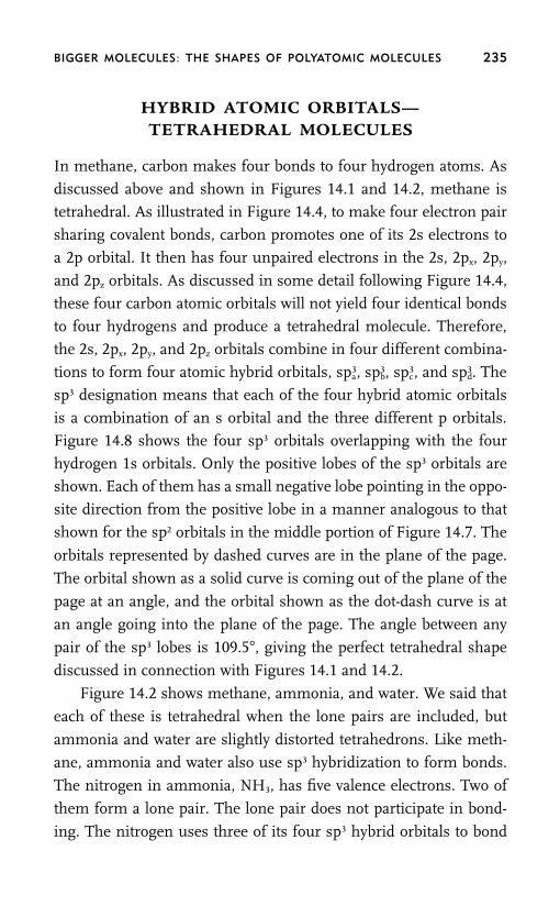
BIGGER MOLECULES: THE SHAPES OF POLYATOMIC MOLECULES 235
HYBRID ATOMIC ORBITALS—TETRAHEDRAL MOLECULES
In methane, carbon makes four bonds to four hydrogen atoms. As
discussed above and shown in Figures 14.1 and 14.2, methane is
tetrahedral. As illustrated in Figure 14.4, to make four electron pair
sharing covalent bonds, carbon promotes one of its 2s electrons to
a 2p orbital. It then has four unpaired electrons in the 2s, 2px, 2py,
and 2pz orbitals. As discussed in some detail following Figure 14.4,
these four carbon atomic orbitals will not yield four identical bonds
to four hydrogens and produce a tetrahedral molecule. Therefore,
the 2s, 2px, 2py, and 2pz orbitals combine in four different combina-
tions to form four atomic hybrid orbitals, sp3a, sp3
b, sp3c, and sp3
d. The
sp3 designation means that each of the four hybrid atomic orbitals
is a combination of an s orbital and the three different p orbitals.
Figure 14.8 shows the four sp3 orbitals overlapping with the four
hydrogen 1s orbitals. Only the positive lobes of the sp3 orbitals are
shown. Each of them has a small negative lobe pointing in the oppo-
site direction from the positive lobe in a manner analogous to that
shown for the sp2 orbitals in the middle portion of Figure 14.7. The
orbitals represented by dashed curves are in the plane of the page.
The orbital shown as a solid curve is coming out of the plane of the
page at an angle, and the orbital shown as the dot-dash curve is at
an angle going into the plane of the page. The angle between any
pair of the sp3 lobes is 109.5�, giving the perfect tetrahedral shape
discussed in connection with Figures 14.1 and 14.2.
Figure 14.2 shows methane, ammonia, and water. We said that
each of these is tetrahedral when the lone pairs are included, but
ammonia and water are slightly distorted tetrahedrons. Like meth-
ane, ammonia and water also use sp3 hybridization to form bonds.
The nitrogen in ammonia, NH3, has five valence electrons. Two of
them form a lone pair. The lone pair does not participate in bond-
ing. The nitrogen uses three of its four sp3 hybrid orbitals to bond

236 ABSOLUTELY SMALL
FIGURE 14.8. Four carbon sp3 hybrid atomic orbitals and four hydro-
gen 1s orbitals for carbon bonding to four hydrogens in methane.
Dashed orbitals in the plane of the page. Solid orbitals out of the
plane. Dot-dash orbitals into the plane. Only the positive lobes of
the sp3 hybrids are shown. The four sp3 hybrids form a perfect tetrahe-
dron.
+
++
++ +
+
+
1s
1s1s
1s
to the three H atoms. The fourth sp3 orbital contains the lone pair.As discussed, the H-N-H bond angle is a little less than the perfect
tetrahedral angle, 109.5�, because the spatial distribution of the lone
pair electrons is somewhat fatter than the N-H bond pair electrons,
and the fatter lone pair pushes the N-H bonds slightly toward each
other. The oxygen in water, H2O, has six valence electrons. Four of
them form two lone pairs. These two lone pairs of electrons do not
participate in bonding. Oxygen uses two of its sp3 hybrid orbitals toform bonds to the two hydrogens. The other two sp3 orbitals are
each occupied by a lone pair. These lone pairs cause the H-O-H
angle to be less than the perfect tetrahedral angle of 109.5� (see
Figure 14.2).
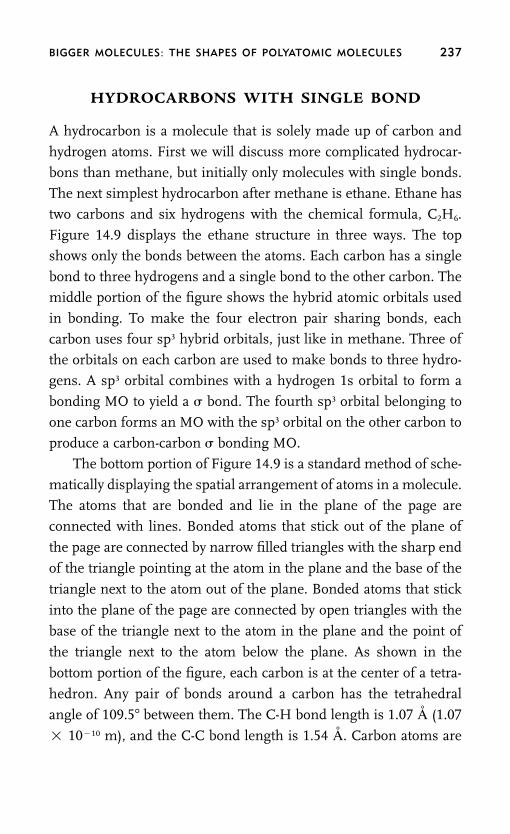
BIGGER MOLECULES: THE SHAPES OF POLYATOMIC MOLECULES 237
HYDROCARBONS WITH SINGLE BOND
A hydrocarbon is a molecule that is solely made up of carbon and
hydrogen atoms. First we will discuss more complicated hydrocar-
bons than methane, but initially only molecules with single bonds.
The next simplest hydrocarbon after methane is ethane. Ethane has
two carbons and six hydrogens with the chemical formula, C2H6.
Figure 14.9 displays the ethane structure in three ways. The top
shows only the bonds between the atoms. Each carbon has a single
bond to three hydrogens and a single bond to the other carbon. The
middle portion of the figure shows the hybrid atomic orbitals used
in bonding. To make the four electron pair sharing bonds, each
carbon uses four sp3 hybrid orbitals, just like in methane. Three of
the orbitals on each carbon are used to make bonds to three hydro-
gens. A sp3 orbital combines with a hydrogen 1s orbital to form a
bonding MO to yield a � bond. The fourth sp3 orbital belonging to
one carbon forms an MO with the sp3 orbital on the other carbon to
produce a carbon-carbon � bonding MO.
The bottom portion of Figure 14.9 is a standard method of sche-
matically displaying the spatial arrangement of atoms in a molecule.
The atoms that are bonded and lie in the plane of the page are
connected with lines. Bonded atoms that stick out of the plane of
the page are connected by narrow filled triangles with the sharp end
of the triangle pointing at the atom in the plane and the base of the
triangle next to the atom out of the plane. Bonded atoms that stick
into the plane of the page are connected by open triangles with the
base of the triangle next to the atom in the plane and the point of
the triangle next to the atom below the plane. As shown in the
bottom portion of the figure, each carbon is at the center of a tetra-
hedron. Any pair of bonds around a carbon has the tetrahedral
angle of 109.5� between them. The C-H bond length is 1.07 A (1.07
� 10�10 m), and the C-C bond length is 1.54 A. Carbon atoms are

238 ABSOLUTELY SMALL
FIGURE 14.9. Three diagrams of ethane, C2H6. Top: The bonds be-
tween atoms. Middle: Each carbon has four sp3 hybrid atomic orbit-
als, three bond to hydrogens and the fourth to the other carbon.
Solid lines: in the plane of the page; dashed lines: out of the plane;
dotted lines: into the plane. Bottom: Method for showing spatial ar-
rangement. Lines: in the plane of the page; filled triangles stick out of
the page; open triangles stick into the page. Each carbon’s bonds are
tetrahedral, with bond angles 109.5�. The C-C bond is longer than the
C-H bonds.
H–C–C–HHH
HH
C
H
H
H
C H
H
HR = 1.07 Å
R = 1.54 Å
109.5°109.5°
C
H
H
H C
H
H
H
sp3

BIGGER MOLECULES: THE SHAPES OF POLYATOMIC MOLECULES 239
bigger than hydrogen atoms, so the separation of the atomic centers
is greater for the two carbon atoms than for a C and an H.
Figure 14.10 shows a ball-and-stick model (top) and a space fill-
ing model (bottom) of ethane. In Figures 14.9 and 14.10, we have
FIGURE 14.10. Ethane ball-and-stick model (top), space-filling model
(bottom). The atoms are the same size in the two models.

240 ABSOLUTELY SMALL
five different representations of the ethane molecule. Only the spac-
ing-filling molecule gives a real feel for the spatial nature of the
molecule. The other four representations exaggerate the separations
between the atoms for clarity. The atoms in the ball-and-stick and
spacing-filling models in Figure 14.10 are the same sizes. In the
ball-and-stick model, the bonds are shown as cylinders, and the
atoms are separated by the bonds. It is important to recognize thatthe bonding comes from the formation of molecular orbitals. The
electrons are shared by the atoms, which are not separated as in the
ball-and-stick model or the other representations. The surface in the
space-filling model contains a large fraction of the electron probabil-
ity distribution. In the space-filling model, the atoms are shaded
differently so that they can be distinguished.
We need to discuss one more relatively simple molecule, pro-pane, before the molecules get large enough that some general fea-
tures can be brought out. Propane has three carbon atoms and eight
hydrogens. Its chemical formula is C3H8. The formula doesn’t tell
how the atoms are connected. It can also be written as H3C-H2C-
CH3. In this notation, it is understood that the hydrogens are
bonded to a carbon. The carbons are bonded to each other with
single bonds. The end carbons are bonded to three hydrogens andanother carbon. The center carbon is bonded to two hydrogens and
two carbons. Figure 14.11 shows two representations of propane.
The top diagram shows the bonding and angles between the bonds.
Each carbon uses four sp3 hybrid orbitals to make four � bonds.
The carbons are tetrahedral, with the C-C-C angle 109.5� and the
HCH angles 109.5�. The bottom portion of the figure shows a ball-
and-stick model of propane.
LARGE HYDROCARBONS HAVEMULTIPLE STRUCTURES
Methane, ethane, and propane have only one way that the atoms
can be bonded together and only on spatial conformation. Butane

BIGGER MOLECULES: THE SHAPES OF POLYATOMIC MOLECULES 241
FIGURE 14.11. A diagram and a ball-and-stick model of propane, C3H8.
The carbon centers are tetrahedral.
C
C
C
H
H
H
H
HH
H H109.5°
109.5°109.5°
and all larger hydrocarbons have multiple structural configurations(the way the atoms are bonded together) and more than one spatial
configuration for a particular structural configuration. Butane has
four carbons. Its chemical formula is C4H10. There are two distinct
structural forms of butane. These are called structural isomers. Fig-
ure 14.12 displays the two structural isomers of butane. Both mole-
cules have the same number of carbons and hydrogens, but they
have very different shapes. Butane can be n-butane, which is nor-mal butane. If we take propane and add one more carbon on the
end, we get n-butane. n-butane is referred to as a linear chain be-
cause a carbon is at most bonded to two other carbons, one on
either side. As can be seen in the ball-and-stick model, the molecule
is not actually linear because each carbon has a tetrahedral arrange-
ment of bonds formed using four sp3 hybrid orbitals.

242 ABSOLUTELY SMALL
FIGURE 14.12. Two structural isomers of butane, C4H10. In the diagram
at the top, CH3 represents a carbon bonded to three hydrogens. N-butane
is a linear chain in the sense that each carbon is bonded to at most two
other carbons. Isobutane is branched. The central carbon is bonded to
three other carbons.
CH 3
H3C C CH 3
H
n-butane isobutane
H3C C C CH 3
H H
H H
As shown in Figure 14.12, butane can have another isomer,
called isobutane. Isobutane has a central carbon connected to three
other carbons and one hydrogen, with each of the other three car-
bons only connected to the central carbon and to three hydrogens.
All four carbons use sp3 hybrid atomic orbitals for bonding and aretetrahedral. Isobutane is referred to as branched. The fact that bu-
tane can have the same number of carbons and hydrogens but two
different structures is of great importance. Molecules with more
carbon atoms can have many more than two structures.
In addition to the two structural isomers, n-butane has two con-
formers. Conformers are different shapes, conformations, for the
same set of atoms that are connected in the same way. They differbecause it is possible for rotation to occur about a C-C single bond.
Figure 14.13 shows n-butane in two conformations called trans andgauche. Both conformers shown in the figure are n-butane because

BIGGER MOLECULES: THE SHAPES OF POLYATOMIC MOLECULES 243
FIGURE 14.13. Two conformers of n-butane. The gauche form is ob-
tained from the trans form by a 120� rotation about the center C-C bond.
n-butane
trans
gauche
the carbon atoms are connected in the same way. If you take the top
conformer and rotate the central carbon-carbon bond, as shown by
the arrow, 120�, you get the gauche form. The trans conformer has
all of the carbons in a plane. The gauche form has three of the
carbons in a plane and the fourth carbon is sticking out of the plane
of the page. There is actually another gauche form that comes from
rotating the trans form around the central C-C bond 120� in the
opposite direction from that shown by the arrow. In that case the
same three carbons are still in the plane, but the fourth carbon is
sticking into the page instead of out of the page. These two gauche
forms in some sense have the same shape, but they are not the

244 ABSOLUTELY SMALL
same. They are like a left hand and a right hand glove. Like the
gloves, these two gauche forms cannot be superimposed on each
other. They are the mirror images of each other. A carbon center
that can have a right hand and left hand form, depending on a
rotation, is said to be chiral.
The rotations about a C-C single bond that takes a molecule
back and forth from trans to gauche can be very fast in a liquid atroom temperature. Recent ultrafast infrared laser experiments and
theory have determined that the gauche-trans interconversion only
takes 50 ps (picoseconds, 10�12 s), or 50 trillionths of a second. So
in a liquid at room temperature, the two forms of butane will be
switching back and forth so fast that it is not possible to isolate
them as distinct molecules.
DOUBLE AND TRIPLE CARBON-CARBON BONDS
While it is very easy for rotation to occur about a C-C single bond,
this is not true for carbon-carbon double or triple bonds. In Chapter
13, we discussed that O2 has a double bond and N2 has a triple bond.
Carbon-carbon bonds can be single, double, or triple. Rotation
about a C-C double or triple bond is virtually impossible. Therefore,double bonds can lock molecules that are the same structural iso-
mers into different conformers. As we will see in Chapter 16, this
is where the term trans fats comes from. However, before we go on
to discuss large molecules, such as trans fats, we first need to talk
about C-C double and triple bonds.
In the carbon compounds discussed so far, carbon uses four sp3
hybrid atomic orbitals to make four single � bonds to other atoms.In such bonding, each carbon has a tetrahedral arrangement of four
bonds. In Figure 14.3, formaldehyde is shown. Formaldehyde has a
carbon with a double bond. To illustrate the manner in which car-
bon can make single, double, and triple bonds, we will take a look
at the bonding in ethane, ethylene, and acetylene. These three com-

BIGGER MOLECULES: THE SHAPES OF POLYATOMIC MOLECULES 245
pounds have chemical formulas, H3C�CH3, H2C�CH2, andHC�CH, respectively. Ethane has a single bond, ethylene has adouble bond, and acetylene has a triple bond. Figure 14.14 showsthe structures of the three molecules. In ethane, each carbon formsfour tetrahedral bonds. In ethylene, each carbon forms three trigo-nal bonds, and in acetylene, each carbon forms two linear bonds.
Although in each of the three molecules the two carbons arebonded to each other, the bond order really makes a difference.Table 14.1 gives the bond orders, C-C bond lengths, and bond ener-
FIGURE 14.14. Ethane, single bond, carbon tetrahedral bonds. Ethylene,
double bond, carbon trigonal bonds. Acetylene, triple bond, carbon linear
bonds.
ethane
ethylene
acetylene

246 ABSOLUTELY SMALL
TABLE 14.1. Single, Double, and Triple C-C Bonds.
bond order C-C bond length C-C energy
ethane single (1) 1.54 A 5.8 � 10�19 J
ethylene double (2) 1.35 A 8.7 � 10�19 J
acetylene triple (3) 1.21 A 16 � 10�19 J
gies of the three molecules. As the bond order increases, the bond
length decreases substantially and the bond energy almost triples
in going from the single to the triple bond.
Carbon-Carbon Double Bond—Ethylene
First let’s look at the bonding in ethylene. As can be seen in Figure
14.15, the carbon centers are trigonal. As discussed, to have trigonal
bonding, a carbon atom will use three sp2 hybrid atomic orbitals to
form bonding MOs (see Figure 14.7). Carbon has four valence
atomic orbitals to use for bonding, 2s, 2px, 2py, and 2pz. In the top
part of the figure, the ethylene molecule is in the xy plane. So the
carbons and the hydrogens are in the plane of the page, which is xy.To form the trigonal sp2 hybrids to make three bonds, each carbon
will use the 2s, 2px, and 2py orbitals. With the three sp2 hybrids,
each carbon will make three � bonds, one to the other carbon and
two to hydrogens. The � bonding is shown in the top portion of
Figure 14.15.
When a carbon forms three sp2 hybrids with the 2s, 2px, and 2py
orbitals, it has its 2pz orbital left over that does no participate in the� bonding. In the top part of Figure 14.15, the 2pz orbitals stick out
of and into the page. Each carbon has one unpaired electron in its
2pz orbital. The bottom portion of the figure shows the ethylene
molecule rotated. The � bonds are shown as the lines connecting
the atoms. The positive lobes of the 2pz orbitals overlap construc-

BIGGER MOLECULES: THE SHAPES OF POLYATOMIC MOLECULES 247
FIGURE 14.15. Ethylene double bond orbitals. Top: Each carbon uses
three sp2 hybrids to make three � bonds in a trigonal configuration. The
page is the xy plane, with z out of the plane. Bottom: Each carbon has a
2pz orbital not used to form the sp2 hybrids. The 2pz orbitals combine to
make a � bonding molecular orbital to give a second bond between the
carbons.
sp2
CC
HH
HH+ +
++
++
++
+ +sp2 sp2
C CH
H
H
H
+ +
2pz 2pz
X
y
tively as do the negative lobes. The two 2pz orbitals combine to makea � bonding molecular orbital, as shown in Figure 13.3. This is a �
bond because there is no electron density along the line connectingthe carbon atomic centers. The net result is that the two carbonatoms have a double bond composed of a � bond formed from a sp2
orbital on each carbon and a � bond formed from a 2pz orbital oneach orbital.
It is not possible for rotation to occur around the carbon-carbondouble bond. Rotation around the bond would require the overlap

248 ABSOLUTELY SMALL
of the two 2pz orbitals to get worse and worse as the angle got bigger
and bigger. For a 90� rotation, the two 2p orbitals would be pointing
perpendicular to each other, and have no overlap. Such a rotation
would break the � bond, which takes a great deal of energy. As
mentioned, measurements and theory have been used to determine
that the time for butane in liquid solution to rotate about the C-C
single bond is about 50 ps. For ethane the time is about 12 ps.
Butane rotates slower than ethane about the single C-C bond be-
cause it has two additional methyl groups (CH3), one on each end
of the central two carbons. If you put ethylene in the same liquid at
room temperature, it can be roughly estimated that it will take about
one hundred billion years to rotate about the double bond because
of the large amount of energy required to break the � bond. There-
fore, for all practical purposes, a double bond (and a triple bond)
prevents rotational isomerization between conformers that differ by
the configuration about the double bond.
Carbon-Carbon Triple Bond—Acetylene
Acetylene forms a triple bond between the carbons in a manor ana-
logous to the double bond formation in ethylene. Each carbon has
four atomic orbitals, 2s, 2px, 2py, and 2pz, to use in bonding. Acety-
lene is linear (see Figure 14.14). Take the line of the molecule to be
the x axis. Then, each carbon will form two sp hybrids from its 2s
and 2px orbitals. The two sp hybrids on a carbon will be used to
make two � bonds, one to the other carbon and one to a hydrogen.
That leaves two unused 2p orbitals on each carbon, the 2py and the
2pz. The 2pz orbitals on each carbon form one � bonding MO, and
the 2py orbitals on each carbon form another � bonding MO. The
result is that the two carbons have a triple bond, one � bond and
two � bonds.
In the next several chapters, we will discuss a number of impor-
tant types of molecules, for example, alcohols, organic acids, large

BIGGER MOLECULES: THE SHAPES OF POLYATOMIC MOLECULES 249
hydrocarbons, and carbon containing fuels, that is, coal, oil, and
natural gas. Small alcohols are discussed so that we can see what
an alcohol is and how small differences in structure really matter if
you decide to drink something other than ethanol (the alcohol in
beer). The ideas will show why some molecules dissolve in water
while others don’t, and how soap (a type of large organic molecule)
makes insoluble grease dissolve in water. We will examine the im-portance of the inability of double bonds to undergo rotational
structural change in connection with fats and trans fats. What hap-
pens when carbon-based fuels are burned will be described, and
why, for a given amount of energy produced, one fuel produces
more of the greenhouse gas carbon dioxide than another. It is well
known that carbon dioxide is a greenhouse gas, but why? We will
see how the combination of two fundamental quantum mechanicaleffects makes carbon dioxide a potent greenhouse gas.

15
Beer and Soap
IN THIS CHAPTER, we will look at several types of molecules to see
how differences in their nature influence chemical processes.
First, alcohols will be introduced. An alcohol is an organic mole-
cule that contains a particular type of chemical group. An alcohol
can be a relatively small molecule, such as ethyl alcohol, which
chemists usually call ethanol. Ethanol is the alcohol in beer, wine,and vodka. However, large important biological molecules, such
as cholesterol, are also alcohols. We will get to such large mole-
cules in Chapter 16. We will see why ethanol dissolves in water,
how it can turn into vinegar, and outline the chemical reactions
in your body that makes methanol (wood alcohol) poisonous, but
ethanol safe, at least in moderation. Building on the mechanism
that enables some molecules to dissolve in water, we will take alook at the structure of soap and oil molecules to see why you need
soap to take grease off of your dishes and get it to wash down the
drain.
250

BEER AND SOAP 251
ALCOHOLS
Ethanol is ethane (Figure 14.10) with one of the hydrogens replacedby an OH group. The OH group is called a hydroxyl group. The
chemical formula for ethanol is H3CH2COH. Figure 15.1 shows a
diagram and a ball-and-stick model of ethanol. In ethanol as in eth-
ane, the carbon atoms use four sp3 hybrid orbitals to form tetrahe-
dral bonds. The oxygen also uses four sp3 hybrids. One of them is
used to make the bond to the carbon, one is used to bond to the
hydrogen, and the other two contain electron lone pairs. The lonepairs are not shown in the ball-and-stick model in Figure 15.1. (Fig-
ure 14.2 shows the oxygen lone pairs for the water molecule.)
Note that in the ball-and-stick model of ethanol, the hydrogen
that is bonded to the oxygen is considerably smaller than the hydro-
FIGURE 15.1. Ethanol (ethyl alcohol) diagram showing atom connectiv-
ity (top), ball-and-stick model (bottom). The hydrogens are light gray,
the carbons are dark gray, and the oxygen is black.
H– C– C– O– H H
H
H
H

252 ABSOLUTELY SMALL
gens bonded to the carbons. Going back to the Periodic Table
(Chapter 11), we know that oxygen really wants to pick up electrons
to obtain the neon closed shell configuration. It gains the electrons
by making covalent electron pair sharing bonds. However, the shar-
ing is not completely equal in a bond between oxygen and hydro-
gen. The oxygen has a very strong attraction for electrons, so it pulls
some extra electron density away from the hydrogen. The extra elec-tron density on the oxygen makes it a little bit negative and the loss
of electron density makes the hydrogen a little bit positive. This loss
of electron density reduces the size of the electron cloud of hydro-
gen, which is represented by the reduced size of sphere that repre-
sents the hydrogen bonded to the oxygen. Carbon and hydrogen
have almost the identical attraction for electrons when they make a
covalent bond. They share the electrons almost equally. Thus onaverage, there is more electron density on a hydrogen bound to a
carbon than on a hydrogen bound to an oxygen. In general, an alco-
hol is a molecule that has a carbon with an OH group and that
carbon is also bonded only to hydrogens or other carbons.
ETHANOL IS A LIQUID ATROOM TEMPERATURE, NOT A GAS
At room temperature, ethane is a gas but ethanol is a liquid. You
have to make ethane colder than �89� C (�128� F) before it be-
comes a liquid, and you have to make ethanol hotter than 78� C
(172� F) before it boils and goes from a liquid to a gas. Ethane and
larger hydrocarbons like oil do not dissolve in water, whereas etha-
nol and larger alcohols do dissolve in water. Ethane and ethanol arealmost the same size, and they have similar shapes. So why, in
contrast to ethane, does ethanol dissolve in water, and why is it a
liquid at room temperature?
As we briefly discussed, ethanol’s hydroxyl group, the OH, has
two partial changes. The O is a little bit negative, and the H is a little

BEER AND SOAP 253
bit positive. A diagram showing the partial charges is: O���H��. The
� (Greek letter delta) is used to mean ‘‘a little bit.’’ The � is followed
by the sign of the electrical charge on the atom. The amount of
electron density transferred from the H to the O is very small, much
less than one full electron that is transferred in a salt like NaCl,
which is Na� and Cl�. The bond between the oxygen and the hydro-
gen is mainly covalent, not ionic as in NaCl. However, the partialcharges on the O and H are unbelievably important. They result
from the details of the quantum mechanical molecular orbitals re-
sponsible for the oxygen-hydrogen covalent bond. These partial
charges result in ethanol being a liquid. If you will permit only mild
hyperbole, without the same type of partial charges on the oxygen
and hydrogen atoms of water molecules, life would not exist.
Ethanol is a liquid because the partial changes give rise to a typeof chemical interaction between molecules called hydrogen bonds.
Hydrogen bonds are much weaker than a real covalent chemical
bond. They are about a 10th the strength or less. While an accurate
description of hydrogen bond formation requires quantum theory,
a qualitative understanding can be obtained by considering electro-
static interactions between partial charges. A hydrogen bond is
formed when the slightly positive H on one molecule is attracted tothe slightly negative O on a different molecule. That attraction will
tend to maintain the H of one ethanol in a pretty well-defined posi-
tion relative to the O of another ethanol. These attractions hold the
ethanols together to form a liquid at room temperature. Ethane mol-
ecules do not have these relatively strong intermolecular attractions.
Heat is a form of kinetic energy. Heat jiggles the molecules
around. In ethane, the molecules do not have a substantial attrac-tion of one for another. At room temperature, the heat-induced mo-
tions cause ethane molecules to fly apart, so ethane is a gas. Imagine
you and another person hold hands and run in opposite directions.
If you hold hands weakly, you will fly apart and take off in different
directions, like ethane molecules. If you hold hands very tightly, the

254 ABSOLUTELY SMALL
two of you will stay together, but move around somewhat as you tug
each other to and fro, like ethanol molecules.
Figure 15.2 shows four ethanol molecules hydrogen bonded to-
gether into a chain. The dashed lines go from the hydrogen of the
OH group of one ethanol to a lone pair on an oxygen of another
ethanol. The lone pair has a good deal of electron density, so the
FIGURE 15.2. Four ethanol molecules that form a chain. The oxygens
are almost black in the figure. An oxygen has two lone pairs in addition
to the hydrogen and carbon bonded to it. The dashed lines show hydrogen
bonds that go from the hydroxyl’s H on one ethanol to an oxygen lone
pair on another ethanol.

BEER AND SOAP 255
slightly positive H is attracted to the electrons of a lone pair on
oxygen. This continues from one ethanol to another to form chains.
Ethanol liquid is composed of hydrogen-bonded chains that hold
the molecules together. The hydrogen bonds make ethanol a liquid
at room temperature, but they are relatively weak. These bonds are
constantly being broken and reformed, but on average, each ethanol
has hydrogen bonds (H-bonds) to one or more other ethanols. How-ever, if you heat the ethanol up enough, the thermally (heat) in-
duced jiggling causes the molecules to break the H-bonds and fly
apart. The temperature at which the thermal energy is enough to
cause the ethanols to fly apart is the boiling point (78� C). At this
temperature or above, ethanol is a gas.
WATER MAKES HYDROGEN BONDS
Back to why hydrogen bonds are necessary for life. Water, H2O, is a
very small molecule. It has a molecular weight that is similar to that
of oxygen (O2), nitrogen (N2), or methane (CH4), all of which are
gases at room temperature. Water has a single oxygen bonded to
two hydrogens. Like the situation in ethanol, the oxygen makes co-
valent bonds to the hydrogens, but in an O-H covalent bond, theelectrons are not shared perfectly equally. In a water molecule, the
oxygen withdraws some electron density from the H’s. A diagram
of water showing this is: H���O���H ��. The slightly positive hy-
drogens on one water molecule are attracted to the slightly negative
oxygens on another water molecule. One water molecule can make
up to four hydrogen bonds.
A schematic illustration of water hydrogen bonding is shown inFigure 15.3. The central water molecule is making four hydrogen
bonds with the surrounding four waters. The central water’s two
hydroxyls are hydrogen bonded to two oxygens of other water mole-
cules. And two other water molecules’ hydroxyls are forming hydro-
gen bonds with the oxygen of the central water. In contrast to the

256 ABSOLUTELY SMALL
FIGURE 15.3. A central water molecule hydrogen bonded to four sur-
rounding water molecules. The central water’s two hydroxyl hydrogens
bond to two oxygens, and the central water’s oxygen accepts two hydroxyl
bonds from two other water molecules.
depiction in Figure 15.3, the hydrogen bonding does not stop with
the five water molecules. The outer four water molecules will each
make approximately four hydrogen bonds with other water mole-
cules. The result is a hydrogen bonding network.
At room temperature, there is enough heat so that hydrogen
bonds between water molecules are continually breaking and new
hydrogen bonds are formed with different water molecules. So the
hydrogen bond network is not static. It is continually reforming and
rearranging. The time scale for these hydrogen bond rearrange-
ments has been measured with ultrafast infrared spectroscopy,
and it is approximately 3 ps (picosecond, a trillionth of a second,
10�12 s).
Life is based on chemistry that occurs in water. Recent space-

BEER AND SOAP 257
craft sent to Mars are not looking directly for signs of past life, but
rather for signs of past liquid water. Liquid water is so fundamental
to life that its presence is a necessary and perhaps a sufficient condi-
tion for life to exist. Water’s amazing properties, which are essential
to the biochemistry of life, are a result of its hydrogen bonding
network structure and the ability of that structure to rearrange. Wa-
ter’s properties allow it to accommodate a vast array of chemicalprocesses necessary for life. For example, proteins fold in water.
Proteins are the very large, extremely complex molecules that are
responsible for most of the chemical processes in our bodies. When
proteins are chemically produced by other proteins, initially they are
not in the correct configuration to function. This is called unfolded.
Proteins have regions that will readily form hydrogen bonds to
water and regions that are more like hydrocarbon and do not wantto mix with water. The protein rearranges its structure, folds, such
that the hydrophilic (likes water) regions are on the outside exposed
to water and form hydrogen bonds with water and the hydrophobic
(dislikes water) regions are on the inside away from water. Such
selective interactions with water are an important driving force that
helps proteins to obtain the correct shapes necessary to function. It
is because water can readily reform its network structure throughthe making and breaking of hydrogen bonds that it can accommo-
date the proteins’ structural transformation and a vast number of
other chemical processes that occur in living organisms.
WATER IS A GREAT SOLVENT
One of water’s properties is its ability to dissolve a very wide varietyof chemical compounds. We have discussed that NaCl will dissolve
in water to give ions, Na� and Cl�. The positive ions are surrounded
by the slightly negative oxygens of water, and the negative ions are
surrounded by the slightly positive hydrogens of water. Salt dis-
solves because of water’s ability to interact favorably with both cat-

258 ABSOLUTELY SMALL
ions and anions. Water can also dissolve a very wide variety of
organic compounds. Water will not dissolve hydrocarbons such as
ethane, but it will dissolve organic molecules like ethanol that have
hydroxyl groups (�OH) or other groups that have slightly charged
or fully charged portions. Water dissolves ethanol by forming hydro-
gen bonds to the hydroxyl group of ethanol. In pure ethanol, ethanol
molecules hydrogen bond one to another to form chains, as shownin Figure 15.2. When ethanol is put in water, water can form hydro-
gen bonds to ethanol’s hydroxyl, incorporating ethanol molecules
into water’s hydrogen bonding network. Vodka is essentially ethanol
in water. Wine is water with less ethanol in it than vodka. Wine also
has large organic molecules that give red wine its color and all wines
their distinct aroma and taste.
ETHANOL WILL UNDERGO CHEMICALREACTIONS WITH OXYGEN
If wine is exposed to air for too long, it will ‘‘go bad’’ and turn into
vinegar. Vinegar is made by purposely making wine go bad. The
chemical reactions that convert wine into vinegar are actually facili-
tated by a bacteria, acetobacter, which has the ability to convert etha-
nol into acetic acid when oxygen is present. The process requires
two chemical reaction steps. The chemical reactions are written as
CH3CH2OH V CH3CHO � H2
2CH3CHO � O2 V 2CH3COOH
First ethanol (CH3CH2OH) is converted to acetaldehyde(CH3CHO) and hydrogen gas (top line), and then two molecules
of acetaldehyde and one oxygen molecule (two oxygen atoms) are
converted into two molecules of acetic acid (CH3COOH), which is
vinegar. The structure of ethanol is shown in Figure 15.1. The struc-
tures of acetaldehyde (top) and acetic acid (bottom) are shown in

BEER AND SOAP 259
Figure 15.4. In both acetaldehyde and acetic acid, the carbon labeledC1 forms a methyl group. C1 is bonded to three hydrogens andcarbon C2. Acetaldehyde has C2 also bonded to a single hydrogenand double bonded to an oxygen. In general, an aldehyde has acarbon double bonded to an oxygen, bonded to a hydrogen, andbonded to another carbon. In formaldehyde (Figure 14.3), insteadof bonding to another carbon, C2 is bonded to a second hydrogen.C2 uses three sp2 hybrid orbitals to form three � bonds and anadditional 2p orbital to combine with a 2p orbital on the oxygen toform a � bond to make the double bond. As shown in the top line
FIGURE 15.4. Acetaldehyde (top) and acetic acid (bottom). Oxygens are
the almost black spheres. Acetaldehyde C2 carbon is bonded to C1, a
hydrogen, and double bonded to an oxygen. Acetic acid C2 is bonded to
C1, double bonded to an oxygen and single bonded to another oxygen
that is part of a hydroxyl group.
C2
C1
C1
C2

260 ABSOLUTELY SMALL
of the chemical reaction equations and looking at the structure of
ethanol in Figure 15.1, ethanol goes to acetaldehyde by eliminating
two hydrogen atoms to give acetaldehyde and an H2 molecule. Two
molecules of acetaldehyde each pick up one oxygen atom from O2
to yield two acetic acid molecules (bottom of Figure 15.4). Acetic
acid has C2 bonded to two oxygen atoms. C2 is double bonded to
one and single bonded to the oxygen of the hydroxyl group �OH.Acetic acid is an organic acid, also called a carboxylic acid. The
�COOH is the acid group. The simplest definition of an acid is a
chemical that when put in water results in the generation of hydro-
gen ions, H�. Hydrochloric acid is HCl. Like NaCl, when put in
water HCl comes apart to give H� and Cl� ions. HCl dissociates
into ions completely. It is called a strong acid because for every
molecule of HCl put in water, you get one H� ion. The H� will beassociated with (solvated by) water molecules. The slightly negative
oxygens of water molecules surround the H�. The acid dissociation
reaction of acetic acid in water can be written in the following
manner.
The �COOH group is the organic acid group. This group ion-izes to give �COO� � H� as shown. The diagram indicates that
the negative charge is stuck on one of the oxygens. In fact, it is
shared equally by both oxygens. This equal sharing is represented
by the following diagram.

BEER AND SOAP 261
The dashed curve indicates that the molecular orbital that con-
tains the electron that gives rise to the negative charge is spread out
over both oxygens. Each oxygen can be thought of as having one-
half of a negative charge. Organic acids are very soluble in water.
Ethanol is soluble because the hydroxyl oxygen has a small negative
charge that leads to hydrogen bond formation with water molecules.
Nondissociated acetic acid has two oxygens with partial charges thatcan hydrogen bond to water. Dissociated acetic acid has two oxy-
gens, each with a half negative charge that readily hydrogen bonds
to water.
Organic acids, such as acidic acid, are weak acids. In water, only
a small fraction of the acetic acid molecules ionize to produce H�
and acetate anion. If you have 60 grams of acidic acid in a liter of
water, which is about four tablespoons (2 ounces) in a quart ofwater, only about 0.4% of the acidic acid molecules will be ionized
to produce H� and acetate anion. This concentration, four table-
spoons of acetic acid in a quart of water, is approximately the con-
centration of acetic acid in common vinegar. It is the acetic acid that
gives vinegar its snappy taste. Organic acids are very common in
chemistry and biology. All proteins are composed of combinations
of 20 amino acids. Prior to reactions to form a protein, each aminoacid is a type of organic acid containing the organic acid group
�COOH.
METHANOL IS VERY POISONOUS
Methanol is the smallest alcohol molecule. Ethanol is ethane with
one hydrogen replaced by a hydroxyl group, �OH. Methanol ismethane with one hydrogen replaced by a hydroxyl. While ethanol
can be ingested in reasonable quantities without dire consequences,
methanol is highly toxic. Methanol, also called wood alcohol, is a
common contaminant of moonshine liquor. As little as 20 ml (milli-
liters) has been known to cause death, and 15 ml can cause blind-

262 ABSOLUTELY SMALL
ness. Fifteen ml is one tablespoon. Two tablespoons are about one
ounce of liquid. Eight ounces of wine contain about one ounce of
ethanol. So replacing the ethanol with methanol in a class of wine
can cause blindness and death. This is rather remarkable since etha-
nol is just methanol with one additional methyl group (�CH3).
It is not methanol itself that is poisonous, but rather the meta-
bolic products of methanol. In humans and other living organisms,alcohols are converted to other chemicals by enzymes (proteins that
are responsible for chemical reactions) called alcohol dehydroge-
nases. In humans, these enzymes are found in the liver and the
lining of the stomach. The evolutionary development of these en-
zymes probably occurred to break down alcohols that are produced
by bacteria in the digestive tract or to break down alcohols that are
natural components of some foods. Ethanol is converted first toacetaldehyde and then to acetic acid as discussed in connection with
Figure 15.4 above, which shows the structures of these two mole-
cules. Acetaldehyde and acetic acid are not harmful to the body and
can be readily eliminated. Larger alcohol molecules are also con-
verted first to aldehydes and then to organic acids, which can be
eliminated from the body without harm. However, alcohol dehydro-
genases convert methanol to formaldehyde and then to formic acid.The structure of formaldehyde is shown in Figure 14.3. Formalde-
hyde is like acetaldehyde except carbon C2 of acetaldehyde (Figure
15.4, top) is bonded to a single hydrogen rather than to a methyl
group (C1 in Figure 15.4). Formic acid is like acetic acid (Figure
15.4, bottom) but again with C2 bonded to a hydrogen rather than a
methyl group. Formaldehyde in particular, but also formic acid, are
highly toxic. They damage the retina and the optic nerve, leadingto vision impairment and blindness. However, formic acid also is
responsible for serious acidosis, which involves interfering with en-
zymes that break down carbohydrates. Relatively low concentrations
of formaldehyde and formic acid, as well as other metabolites de-
rived from them, can cause death.

BEER AND SOAP 263
SOAP
As we discussed, alcohols like ethanol and organic acids, such asacetic acid, are very soluble in water because the organic groupscontaining oxygens can form hydrogen bonds with water. In con-trast, ethane, which is very similar to ethanol, does not dissolve inwater, because it does not have oxygen containing groups that canform hydrogen bonds. Ethane is a hydrocarbon, that is, it is com-posed only of hydrogens and carbons. Methane and ethane aregases. Larger hydrocarbons, beginning with pentane (five carbons),are liquids at room temperature. The smaller of these liquid hydro-carbons like pentane and octane (a component of gasoline) are verythin liquids, that is, they are not viscous.
LARGE HYDROCARBONS ARE OIL AND GREASE
As the number of carbons increases, the liquid hydrocarbons be-come increasingly viscous. The heating oil, used in homes and busi-nesses in many areas of the United States, is composed of a mixtureof hydrocarbons typically spanning the range of 14 to 20 carbons.At room temperature, oil flows readily but it is much more viscousthan gasoline. Grease is composed of really large hydrocarbons. Itis very viscous and will not pour at room temperature.
The hydrocarbons that comprise heating oil are liquids at roomtemperature, but as discussed, they do not dissolve in water. Mole-cules with 14 carbons are the lightest component of heating oil.Figure 15.5 shows n-tetradecane. Decane has 10 carbons. Tetrade-cane has four (tetra) additional carbons. The n (normal) means thatall of the carbons are connected one to another with no branches.That is, each carbon is connected to at most two other carbons. Theupper portion of the figure shows a ball-and-stick model ofn-tetradecane. It is important to remember that the electron densitysurrounding the atoms in a molecule is space filling. The bottomportion of the figure shows a space-filling model of n-tetradecane.
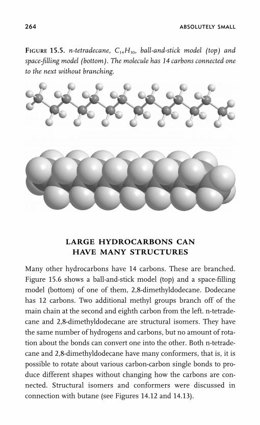
264 ABSOLUTELY SMALL
FIGURE 15.5. n-tetradecane, C14H30, ball-and-stick model (top) and
space-filling model (bottom). The molecule has 14 carbons connected one
to the next without branching.
LARGE HYDROCARBONS CANHAVE MANY STRUCTURES
Many other hydrocarbons have 14 carbons. These are branched.
Figure 15.6 shows a ball-and-stick model (top) and a space-filling
model (bottom) of one of them, 2,8-dimethyldodecane. Dodecane
has 12 carbons. Two additional methyl groups branch off of the
main chain at the second and eighth carbon from the left. n-tetrade-
cane and 2,8-dimethyldodecane are structural isomers. They have
the same number of hydrogens and carbons, but no amount of rota-
tion about the bonds can convert one into the other. Both n-tetrade-
cane and 2,8-dimethyldodecane have many conformers, that is, it is
possible to rotate about various carbon-carbon single bonds to pro-
duce different shapes without changing how the carbons are con-
nected. Structural isomers and conformers were discussed in
connection with butane (see Figures 14.12 and 14.13).

BEER AND SOAP 265
FIGURE 15.6. 2,8-dimethlydodecane, C14H30, ball-and-stick model (top)
and space-filling model (bottom). The molecule has 14 carbons. There is
a chain of 12 carbons, with two methyl groups branching off at the sec-
ond and eighth carbons from the left.
OIL AND WATER DON’T MIX
Heating oil is a relatively viscous liquid, although the hydrocarbon
molecules have relatively weak attractive interactions one for an-
other. The large number of sizes, structural isomers, and conform-
ers cause the molecules to become entangled, which contributes to
the viscosity. If oil is in water, it will float on top. If you shake it up,
it will appear to mix for a while. However, if you let it stand, the oilwill separate and again float on top. Anyone who has made their
own oil-and-vinegar salad dressing knows this. You mix olive oil,
vinegar, and possibly some water, and then you shake it up. If you
let it stand, the olive oil floats right back to the top. In commercial

266 ABSOLUTELY SMALL
oil and vinegar salad dressings, emulsifiers are added to keep the
oil and vinegar from separating. Emulsifiers are very similar to the
soap that we are about to describe. We know that an oxygen atom
in a water molecule is slightly negative and is attracted to atoms
that are positively charged or at least have a partial positive charge.
The hydrogens of water molecules are slightly positive and are at-
tracted to negatively charged or partially negatively charged atoms.Hydrocarbons have carbons and hydrogens that are essentially neu-
tral in charge. Therefore, water molecules are attracted to each other
much more strongly than they are attracted to oil. The result is oil
does not dissolve in water.
THE STRUCTURE OF SOAP MOLECULES
Soap makes oil dissolve in water. Many different molecules are used
as soaps or detergents. The more formal name for a soap molecule
is a surfactant. While the chemical nature and structure of surfac-
tants vary widely, all surfactants have a common feature. A section
of a surfactant molecule, if taken by itself, would be very soluble in
water. The other part of the surfactant molecule by itself would be
very soluble in oil and grease.One such molecule is sodium n-heptadecaneacetate, which is
shown as both a ball-and-stick model and a space-filling model in
Figure 15.7. n-heptadecane is an unbranched 17-carbon chain. This
hydrocarbon portion of the molecule is shown in the figure as a
particular conformer with a couple of rotations about carbon-carbon
bonds that produces the bent shape. Tetradecane, shown in Figure
15.5, is all trans. It does not have any rotations to give some gaucheconformations. Large hydrocarbons have many different conform-
ers that can interconvert. By itself, heptadecane would be one com-
ponent of heating oil.
The n-heptadecane hydrocarbon is attached to an acetate group
or acetate anion. The acetate group comprises the last two carbons
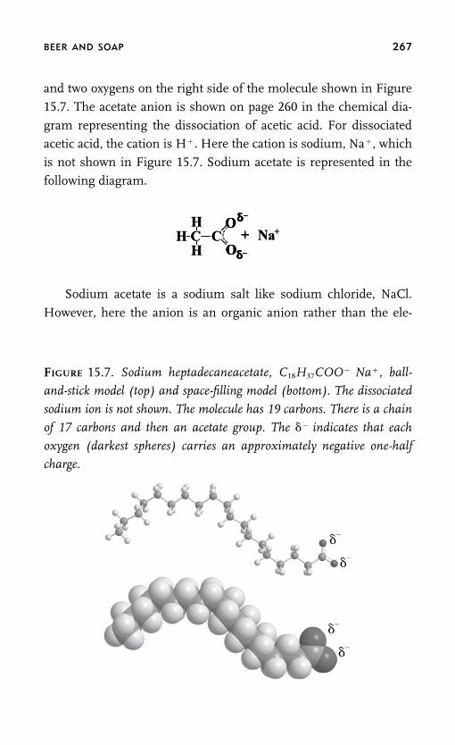
BEER AND SOAP 267
and two oxygens on the right side of the molecule shown in Figure
15.7. The acetate anion is shown on page 260 in the chemical dia-
gram representing the dissociation of acetic acid. For dissociated
acetic acid, the cation is H�. Here the cation is sodium, Na�, which
is not shown in Figure 15.7. Sodium acetate is represented in the
following diagram.
Sodium acetate is a sodium salt like sodium chloride, NaCl.
However, here the anion is an organic anion rather than the ele-
FIGURE 15.7. Sodium heptadecaneacetate, C18H37COO� Na�, ball-
and-stick model (top) and space-filling model (bottom). The dissociated
sodium ion is not shown. The molecule has 19 carbons. There is a chain
of 17 carbons and then an acetate group. The �� indicates that each
oxygen (darkest spheres) carries an approximately negative one-half
charge.
–
–
–
–
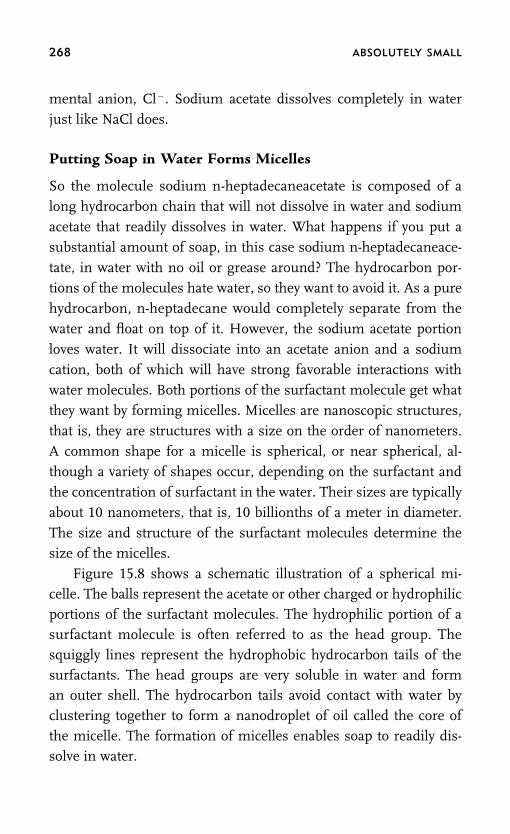
268 ABSOLUTELY SMALL
mental anion, Cl�. Sodium acetate dissolves completely in waterjust like NaCl does.
Putting Soap in Water Forms Micelles
So the molecule sodium n-heptadecaneacetate is composed of along hydrocarbon chain that will not dissolve in water and sodiumacetate that readily dissolves in water. What happens if you put asubstantial amount of soap, in this case sodium n-heptadecaneace-tate, in water with no oil or grease around? The hydrocarbon por-tions of the molecules hate water, so they want to avoid it. As a purehydrocarbon, n-heptadecane would completely separate from thewater and float on top of it. However, the sodium acetate portionloves water. It will dissociate into an acetate anion and a sodiumcation, both of which will have strong favorable interactions withwater molecules. Both portions of the surfactant molecule get whatthey want by forming micelles. Micelles are nanoscopic structures,that is, they are structures with a size on the order of nanometers.A common shape for a micelle is spherical, or near spherical, al-though a variety of shapes occur, depending on the surfactant andthe concentration of surfactant in the water. Their sizes are typicallyabout 10 nanometers, that is, 10 billionths of a meter in diameter.The size and structure of the surfactant molecules determine thesize of the micelles.
Figure 15.8 shows a schematic illustration of a spherical mi-celle. The balls represent the acetate or other charged or hydrophilicportions of the surfactant molecules. The hydrophilic portion of asurfactant molecule is often referred to as the head group. Thesquiggly lines represent the hydrophobic hydrocarbon tails of thesurfactants. The head groups are very soluble in water and forman outer shell. The hydrocarbon tails avoid contact with water byclustering together to form a nanodroplet of oil called the core ofthe micelle. The formation of micelles enables soap to readily dis-solve in water.
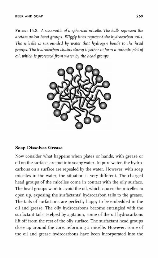
BEER AND SOAP 269
FIGURE 15.8. A schematic of a spherical micelle. The balls represent the
acetate anion head groups. Wiggly lines represent the hydrocarbon tails.
The micelle is surrounded by water that hydrogen bonds to the head
groups. The hydrocarbon chains clump together to form a nanodroplet of
oil, which is protected from water by the head groups.
Soap Dissolves Grease
Now consider what happens when plates or hands, with grease or
oil on the surface, are put into soapy water. In pure water, the hydro-
carbons on a surface are repealed by the water. However, with soap
micelles in the water, the situation is very different. The charged
head groups of the micelles come in contact with the oily surface.
The head groups want to avoid the oil, which causes the micelles to
open up, exposing the surfactants’ hydrocarbon tails to the grease.
The tails of surfactants are perfectly happy to be embedded in the
oil and grease. The oily hydrocarbons become entangled with the
surfactant tails. Helped by agitation, some of the oil hydrocarbons
lift off from the rest of the oily surface. The surfactant head groups
close up around the core, reforming a micelle. However, some of
the oil and grease hydrocarbons have been incorporated into the

270 ABSOLUTELY SMALL
micelle’s core. The containment of hydrocarbons in the interior of
a micelle is shown schematically in Figure 15.9. The hydrocarbon
tails of the surfactants are the double lines, while the oil hydrocar-
bons are single spotted lines. The oil and grease molecules remain
in the micelle core as part of the oil nanodroplet. The additional
hydrocarbons in the core make the micelles bigger. More surfactant
molecules, which are in the water, can join a micelle to fully sur-
round the enlarged oil nanodroplet. The charged head groups of
one micelle repel those of other micelles, which prevents the grease
from coagulating and forming grease globs that are not soluble in
water.
Soap-like materials are reported to have been produced as early
as 2800 bce. True soaps, basically the same as those used today,
were made by chemists in the Islamic world in the seventh century.
Today, we hear a lot about the coming of nanotechnology, in which
nanometer scale assemblies of molecules or atoms can perform
FIGURE 15.9. A schematic of hydrocarbons from oil or grease (single
spotted lines) contained in the interior of a soap micelle.

BEER AND SOAP 271
very specialized functions. It is remarkable that soap in water is a
nanoscopic material. Surfactants form nanometer-size micelles that
can encapsulate grease and oil. The micelles with encapsulated hy-
drocarbons are soluble in water, which makes it possible for us to
wash away otherwise water-insoluble molecules.

16
Fat, It’s All About
the Double Bonds
IN THIS CHAPTER, we will use some of the ideas developed previously
to talk about some of the large molecules commonly discussed in
everyday life. We hear about such things as saturated fats, unsatu-
rated fats, transfats, and cholesterol. What are these things, and
how do they differ? What are the relationships between molecular
structure and health effects?
WHAT IS A FAT MOLECULE?
When we say fat, you may think of butter, lard, olive oil, or cotton-
seed oil. Each of these is actually a mixture of different fats. Figure
16.1 shows one particular molecule that is a fat. It is stearic acid. It
is a long hydrocarbon chain with an organic acid group on the end.Stearic acid has 18 carbon atoms. The end carbon on the right is the
organic acid group. Figure 15.4, bottom, shows acetic acid, which is
an acid group with one methyl attached. Figure 15.5 shows tetrade-
cane, a 14-carbon hydrocarbon, which is a component of heating oil.
Stearic acid is like acetic acid but with a 17-carbon chain attached to
272
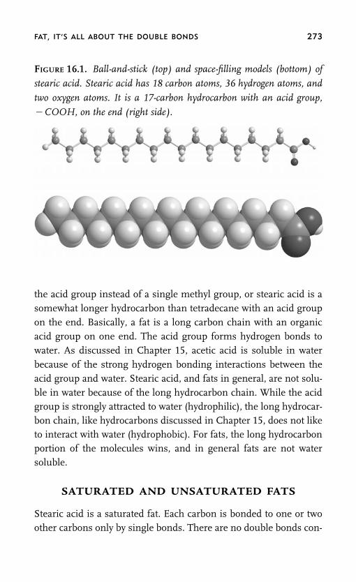
FAT, IT’S ALL ABOUT THE DOUBLE BONDS 273
FIGURE 16.1. Ball-and-stick (top) and space-filling models (bottom) of
stearic acid. Stearic acid has 18 carbon atoms, 36 hydrogen atoms, and
two oxygen atoms. It is a 17-carbon hydrocarbon with an acid group,
�COOH, on the end (right side).
the acid group instead of a single methyl group, or stearic acid is asomewhat longer hydrocarbon than tetradecane with an acid groupon the end. Basically, a fat is a long carbon chain with an organicacid group on one end. The acid group forms hydrogen bonds towater. As discussed in Chapter 15, acetic acid is soluble in waterbecause of the strong hydrogen bonding interactions between theacid group and water. Stearic acid, and fats in general, are not solu-ble in water because of the long hydrocarbon chain. While the acidgroup is strongly attracted to water (hydrophilic), the long hydrocar-bon chain, like hydrocarbons discussed in Chapter 15, does not liketo interact with water (hydrophobic). For fats, the long hydrocarbonportion of the molecules wins, and in general fats are not watersoluble.
SATURATED AND UNSATURATED FATS
Stearic acid is a saturated fat. Each carbon is bonded to one or twoother carbons only by single bonds. There are no double bonds con-

274 ABSOLUTELY SMALL
necting carbon atoms. A saturated fat is a fat with only single bonds
between carbon atoms.
Figure 16.2 shows a ball-and-stick model of oleic acid. Like stea-
ric acid, oleic acid has 18 carbon atoms with an acid group on one
end. However, it has one double bond between carbons 9 and 10,
where the carbon atoms are numbered beginning with the carbox-
ylic acid carbon. Oleic acid is a monounsaturated fat. It is unsatu-
rated because it has a double bond. It is monounsaturated because
it has only one double bond. Saturated fats have no double bonds
between carbon atoms. In stearic acid, except for the carbon in the
acid group, all of the carbons use four sp3 hybrid orbitals to form
bonds. Carbons not at the ends of the stearic acid molecule use two
of the four sp3 hybrid orbitals to form single bonds to the adjacent
carbons and two to bond two hydrogens. Each carbon, except for
the acid carbon, has a tetrahedral arrangement of bonds to other
carbons and hydrogens. Oleic acid’s carbons 9 and 10 use three sp2
hybrids to form three � bonds, one to a hydrogen and two to the
adjacent carbons. Carbons 9 and 10 each use their remaining 2p
orbitals, one on each carbon, to form a � bond between them. So
carbons 9 and 10 have a double bond, and these carbons have a
FIGURE 16.2. Ball-and-stick model of oleic acid. Oleic acid has 18 car-
bon atoms like stearic acid in Figure 16.1, but it has one carbon-carbon
double bond between carbons 9 and 10 counting from the acid group.
double bond
910

FAT, IT’S ALL ABOUT THE DOUBLE BONDS 275
trigonal, rather than a tetrahedral, bonding geometry. The differ-
ence in the geometry can be seen clearly in Figure 14.14 by compar-
ing the model of ethane (carbon-carbon single bond) with ethylene
(carbon-carbon double bond). In ethane, the carbon centers are tet-
rahedral. In ethylene, the carbons are trigonal. Oleic acid has 34
hydrogen atoms in contrast to stearic acid, which has 36 hydrogen
atoms. Oleic acid uses two orbitals to form the double bond that isused in stearic acid to bond hydrogens. A saturated fat has as many
hydrogen atoms as possible, meaning it has no double bonds.
THE SHAPES OF FAT MOLECULES
Stearic acid, as shown in Figure 16.1, is in the all-trans conforma-tion. Figure 14.13 shows butane in the all-trans configuration, with
rotation around one of the bounds to give a gauche conformation.
Stearic acid can assume many conformations besides the all-trans
conformation shown. The all-trans conformation is the most linear,
which is the lowest energy conformation for a saturated hydrocar-
bon or a saturated fat. Because saturated fats only have carbon-car-
bon single bonds, they are constantly interconverting from one
conformer to another. Figure 15.7 displays heptadecaneacetate notin an all-trans configuration. In contrast to stearic acid, oleic acid
(Figure 16.2) is not naturally produced in an all-trans configuration.
In Figure 16.2, the angles made by carbons 8, 9, and 10 and by
carbons 9, 10, and 11 are 120� (trigonal) and not 109.5� (tetrahedral).
Therefore, under normal biological conditions adding one double
bond locks in a particular shape around the double bond.
SATURATED, MONOUNSATURATED, ANDPOLYUNSATURATED FATS
Figure 16.3 is a ball-and-stick model of �-linolenic acid. Like stearic
acid and oleic acid, �-linolenic acid has 18 carbons, but it has three

276 ABSOLUTELY SMALL
FIGURE 16.3. Ball-and-stick model of �-linolenic acid, which has 18 car-
bon atoms and three carbon-carbon double bonds.
double bonds
910
12
1315
16
double bonds. �-linolenic acid is said to be polyunsaturated in thatit has more than one double bond. In linolenic acid, six of the car-bon atoms, specifically 9, 10, 12, 13, 15, and 16, are trigonal, with120� angles formed by three carbon atoms, such as 8, 9, and 10,rather than with 109.5� tetrahedral angles. Under normal condi-tions, these additional double bonds force the shape further awayfrom an all-trans configuration. While �-linolenic acid has threedouble bonds, linolenic acid, which is similar, has only two doublebonds. A fat with no double bonds is saturated. A fat with one dou-ble bond is monounsaturated, and a fat with two or more doublebonds is polyunsaturated.
DOUBLE BONDS IN FATS MATTER
Why does it matter whether or not a fat has double bonds? This isa question that divides into two types of issues, those for chemically

FAT, IT’S ALL ABOUT THE DOUBLE BONDS 277
modified fats and those for nonchemically modified fats contained
in oils and other sources of fat like butter. First, let’s look at fats
that have not been chemically modified. Fats have been correlated
with either increasing or decreasing cholesterol levels. Myristic acid,
which is a saturated fat with 14 carbons, is believed to increase
cholesterol significantly in a deleterious manner. Palmitic acid,
which is a saturated fat with 16 carbons, is thought to increase cho-lesterol to some extent. In contrast, linolenic acid (18 carbons with
two double bonds) and other polyunsaturated fats decrease choles-
terol levels. However, some saturated fats, such as stearic acid (Fig-
ure 16.1), do not appear to have much influence on cholesterol
levels, which is also true of monounsaturated fats such as oleic acid
(Figure 16.2).
In common oils used in food, the fractions of important unsatu-rated and polyunsaturated fats vary widely. Butter fat and coconut
oil contain large amounts of myristic acid and palmitic acid and
very little linolenic acid. Olive oil contains no myristic acid, but it
has a significant amount palmitic acid. It also has some linolenic
acid. Canola oil has no myristic acid and almost no palmitic acid. It
has a substantial amount of linolenic acid. Grape seed oil, safflower
oil, and sunflower oil (the later two when not processed for high-temperature cooking, see below) have no myristic, small amounts
of palmitic, but very large amounts of linolenic acid. The chemical
composition of these fats indicate that butter fat and coconut oil will
have a deleterious effect on blood cholesterol, olive oil is approxi-
mately neutral, canola oil has a positive effect, and grape seed oil,
safflower oil, and sunflower oil (the last two not for high-tempera-
ture cooking) have a very positive effect on blood cholesterol.
CHEMICALLY MODIFIED FATS
Fats are chemically modified for several reasons. Unsaturated fats
are fats with double bonds. Double bonds are chemically very reac-
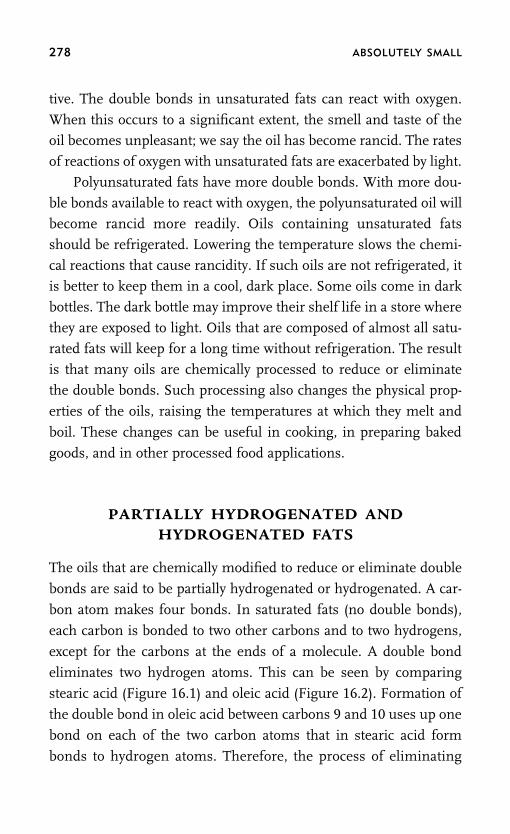
278 ABSOLUTELY SMALL
tive. The double bonds in unsaturated fats can react with oxygen.
When this occurs to a significant extent, the smell and taste of the
oil becomes unpleasant; we say the oil has become rancid. The rates
of reactions of oxygen with unsaturated fats are exacerbated by light.
Polyunsaturated fats have more double bonds. With more dou-
ble bonds available to react with oxygen, the polyunsaturated oil will
become rancid more readily. Oils containing unsaturated fats
should be refrigerated. Lowering the temperature slows the chemi-
cal reactions that cause rancidity. If such oils are not refrigerated, it
is better to keep them in a cool, dark place. Some oils come in dark
bottles. The dark bottle may improve their shelf life in a store where
they are exposed to light. Oils that are composed of almost all satu-
rated fats will keep for a long time without refrigeration. The result
is that many oils are chemically processed to reduce or eliminate
the double bonds. Such processing also changes the physical prop-
erties of the oils, raising the temperatures at which they melt and
boil. These changes can be useful in cooking, in preparing baked
goods, and in other processed food applications.
PARTIALLY HYDROGENATED ANDHYDROGENATED FATS
The oils that are chemically modified to reduce or eliminate double
bonds are said to be partially hydrogenated or hydrogenated. A car-
bon atom makes four bonds. In saturated fats (no double bonds),
each carbon is bonded to two other carbons and to two hydrogens,
except for the carbons at the ends of a molecule. A double bond
eliminates two hydrogen atoms. This can be seen by comparing
stearic acid (Figure 16.1) and oleic acid (Figure 16.2). Formation of
the double bond in oleic acid between carbons 9 and 10 uses up one
bond on each of the two carbon atoms that in stearic acid form
bonds to hydrogen atoms. Therefore, the process of eliminating

FAT, IT’S ALL ABOUT THE DOUBLE BONDS 279
double bonds from a fat increases the number of hydrogen atoms,
and we say the oil has been hydrogenated.
HYDROGENATION OF FATS
Double bonds are very stable, and it is difficult to break a double
bond. The hydrogenation process turns a carbon-carbon doublebond into a carbon-carbon single bond with a hydrogen added to
each carbon. The process requires high temperature, a metallic cata-
lyst, and hydrogen. A catalyst is a material that makes a chemical
reaction occur faster, but the catalyst is not used up in the process.
Qualitatively, the process of hydrogenation works as follows. One
of the carbon atoms of a double bond binds to the metal, essentially
eliminating the double bond. The binding leaves the other carbonatom with an unpaired electron. That carbon atom is now single
bonded to two other carbons and one hydrogen. As we know, a
carbon atom wants to make four bonds to have enough electrons
to obtain the neon closed shell configuration. The carbon grabs a
hydrogen atom. The other carbon atom breaks its bond to the metal
catalyst, and it grabs another hydrogen atom. The carbon-carbon
double bond has been converted to a single bond and two hydrogenatoms have been added to the fat.
For a polyunsaturated fat, this process can be repeated at all of
the double bonds or only at some of them. If it occurs at all of
the double bonds, the polyunsaturated fat has been converted to a
saturated fat; we say the fat has been hydrogenated. If hydrogena-
tion occurs at some but not all of the double bonds, we say the fat
has been partially hydrogenated. The resulting fat may be monoun-saturated or still polyunsaturated but with fewer double bonds. The
degree of hydrogenation is controlled to produce a resulting fat with
the desired properties, particularly whether it is a solid or liquid at
room temperature, the melting temperature, and the boiling tem-
perature.

280 ABSOLUTELY SMALL
READ THE LABEL
As discussed above, polyunsaturated fats can be beneficial. As they
occur naturally, both sunflower oil and safflower oil have very large
percentages of polyunsaturated fats. However, many brands of sun-
flower oil and safflower oil have been partially hydrogenated, so they
are more usable for high-temperature cooking. It is possible to tell
by reading the nutrition label if sunflower oil and safflower oil have
been partially hydrogenated. If the label shows that the amount per
serving of monounsaturated fat is greater than the amount of poly-
unsaturated fat, then the oil has been partially hydrogenated. If
these oils have not been partially hydrogenated, then the amount of
polyunsaturated fat will greatly exceed the amount of monounsatur-
ated fat. So to get the benefits of significant quantities of polyunsat-
urated fat from sunflower or safflower oils, the oils should not be
partially hydrogenated. Reading the label will tell.
TRANS FATS
All of this hydrogenation of oils sounds fine except for one thing;
the big elephant in the room is trans fats. What is a trans fat? Figure
16.4 shows oleic acid in both its cis and trans geometries. Both
molecules have 18 carbons, 34 hydrogens, and one carbon-carbon
double bond. The atoms are connected one to another in the same
order. The difference is the geometry around the double bond.
In the cis conformation, the two hydrogens bonded to carbons
9 and 10 are on the same side of the molecule. They point at an
angle toward the top of the page. The molecule is drawn with the
double bond horizontal. The angle between the double bond and
one of the H atoms is 120� because trigonal sp2 hybrids are used to
make the � bonds. So the angles made by the bonds from carbons
9 and 10 to the hydrogens are 30� from the vertical direction. For

FAT, IT’S ALL ABOUT THE DOUBLE BONDS 281
FIGURE 16.4. Ball-and-stick models of cis-oleic acid and trans-oleic acid.
Both have 18 carbons and one double bond. However, their geometries
differ.
double bond
9
9
10
10
cis-oleic acid
trans-oleic acid
the cis molecule, the two chains of atoms connected to carbons 9
and 10 on either side of the double bond angle downward, again
making angles that are 30� from the vertical line that is perpendicu-
lar to the double bond.
In the trans conformation, the two hydrogens bonded to car-
bons 9 and 10 are on opposite sides of the molecule. One points
almost straight up toward the top of the page and the other points
almost straight down toward the bottom of the page. The two chains
of carbon atoms that are bound to carbons 9 and 10 come out in
opposite directions relative to the double bond. The net result is that
the cis molecule is ‘‘bent’’ around the double bond, while the trans
molecule is ‘‘straight’’ relative to the double bond.
Rotation around a carbon-carbon double bond cannot occur
under normal conditions. The inability of rotation to occur around
double bonds is fundamentally important. Figure 14.13 shows the

282 ABSOLUTELY SMALL
gauche and trans conformations of n-butane, which has only single
bonds. Rotation around single bonds can occur readily at room tem-
perature. Therefore, in the example of n-butane, the gauche and
trans conformations are not fixed. In fact, in liquid solution at room
temperature, the n-butane gauche and trans conformations will in-
terconvert by rotation around the middle carbon-carbon single bond
in approximately 50 ps (50 trillionth of a second), which is a veryshort time. In contrast, the cis and trans conformations of oleic acid
shown in Figure 16.4 are locked in. They will not interconvert with-
out very high temperature and a catalyst.
To understand why rotation around a carbon-carbon single
bond occurs readily while rotation about a double bond does not,
we need to look again at the hybrid orbitals used by carbon to make
single and double carbon-carbon bonds. Figure 14.9 illustrates thehybrid orbitals used in ethane to form the carbon-carbon single
bond. Each carbon bonds to the other atoms using four sp3 hybrid
orbitals. The middle part of Figure 14.9 shows schematically the
formation of the carbon-carbon single bond by the overlap of one
sp3 orbital on each carbon. The two orbitals, one from each carbon,
point right at each other. Rotating one of the carbons does not
change the overlap of the orbitals. There are favored configurationsbecause the hydrogens on the two carbons want to avoid each other
as much as possible, but the molecule can readily rotate from one
favored configuration to another without changing the carbon-
carbon sp3 orbital overlap. This is in contrast to the situation for
ethylene, which has a carbon-carbon double bond. Figure 14.15
shows the orbitals used to form the double bond in ethylene. Each
carbon uses three sp2 hybrids to make � bonds to two hydrogensand the other carbon as shown in the top portion of Figure 14.15.
The three sp2 orbitals on each carbon are formed by superpositions
of the 2s, 2px, and 2py orbitals. These orbitals and the � bonds are
in the plane of the page, which is taken to be the xy plane. That
leaves one 2pz orbital on each carbon atom, which will point perpen-

FAT, IT’S ALL ABOUT THE DOUBLE BONDS 283
dicular to the plane of the page. As shown in the bottom portion of
Figure 14.15, the two 2pz orbitals overlap side to side to form a �
bond. If you could grab one of the carbons and rotate it, you would
be rotating that 2pz orbital away from the z direction toward the xy
plane. Such a rotation will decrease the overlap between the two 2pz
orbitals, breaking the � bond. As shown in the table that follows the
discussion of Figure 13.9, a double bond is much stronger than asingle bond. Therefore, it will take a great deal of energy to rotate
around a carbon-carbon double bond because it is necessary to
break the � bond for the rotation to occur. The large energy penalty
that would be paid prevents rotation.
NATURE PRODUCES CIS FATS BUT CHEMICALPROCESSING PRODUCES TRANS FATS
Unsaturated fats, both monounsaturated and polyunsaturated, are
produced in nature virtually exclusively in cis conformations. Small
amounts of trans fats are found in the meat and milk of cattle,
sheep, goats, and other ruminants. However, large amounts of trans
fats are present in partially hydrogenated oils, and trans fats are also
found in hydrogenated oils because the chemical processing doesnot result in an oil that is 100% saturated. Unprocessed monounsa-
turated and polyunsaturated vegetable oils have only cis conforma-
tions about their double bonds. Partial hydrogenation of the
naturally occurring oils generates large quantities of trans fats. This
transformation from cis to trans occurs during the hydrogenation
process. As discussed above, one of the carbons of a carbon-carbon
double bond binds to a metal catalyst in the reaction vessel, whichis at very high temperature. When bound to the catalyst, the carbon-
carbon bond is effectively a single bond, and rotation from cis to
trans can occur. The oil can break its bond to the catalyst before
hydrogenation occurs, so the double bond is not hydrogenated, and
it reforms. So, rotation from cis to trans can take place before the

284 ABSOLUTELY SMALL
oil is released from the catalyst. If this occurs, the result is the con-
version of a cis conformation to a trans conformation without hydro-
genation of the double bond. The processing is intended to reduce
the number of double bonds, not eliminate all of them. But a sub-
stantial number of double bonds are converted from cis to trans.
The result is that partially hydrogenated oils can contain substantial
fractions of trans double bonds.
TRANS FATS CAN BE DELETERIOUS
Trans fats have been shown to have a number of deleterious health
effects. The basic reason for the harmful effects of trans fats arises
from the fact that biological systems have developed to deal with
cis fats, and shape matters. Enzymes are proteins (large biologicalmolecules) that act as very specific chemical factories. They can con-
vert fats into other useful molecules, as well as break down fats for
elimination. However, an enzyme that will work on a cis fat will, in
general, not produce the same chemical reactions or any reaction at
all for the trans fat, although it has the identical chemical formula.
So two fats that have the identical numbers of carbons, hydrogens,
and oxygens, all connected to each other in the same order, will betreated very differently biochemically depending on whether they
are cis or trans. Our bodies have not evolved to deal with substantial
amounts of trans fats.
Trans fats have been strongly linked to heart disease because of
their effect on cholesterol levels in the blood. Trans fats may also
have a harmful effect on the nervous system. Myelin is a covering
that protects neurons. It is composed of about 30% protein andabout 70% fat. The two main fats are oleic acid (see Figures 16.2
and 16.4) and docosahexaenoic acid (DHA, see below). Trans fats
replace DHA in brain cell membranes and in myelin. Trans fat al-
ters the electrical signals that comprise the messages in the nervous
system, affecting communication between neurons. It is remark-

FAT, IT’S ALL ABOUT THE DOUBLE BONDS 285
able that a change in shape of a molecule, without changing its
chemical composition, can make a beneficial food a harmful food.
WHEN ZERO IS ZERO
Because of the mounting evidence that trans fats are harmful to our
health, they should be avoided. Consumer advocacy groups have
encouraged the required removal of trans fats from cooking oils
used in fast food restaurants and in various commercial products.
Because of the bad publicity surrounding trans fats, manufacturers
try to avoid alerting consumers to their presence. Now that most
people know that partial hydrogenation will produce trans fats,
some food labels use the term modified instead of the phrase ‘‘par-
tially hydrogenated.’’ Even more amazing is the U.S. government’s
definition of 0% trans fat. Government regulations permit a product
label to say that an oil contains 0% trans fat if one serving contains
less than 0.5 grams of trans fat, but the manufacturer is permitted
to define the size of a serving. Let’s say that there are 0.6 grams of
trans fat in a tablespoon of oil. One tablespoon is three teaspoons.
So, the manufacturer defines a serving as two teaspoons, which
contain 0.4 grams of trans fat. Thus, by changing the definition of
a serving, the oil has 0% trans fat. This type of labeling is not per-
mitted in Europe and other countries. Minimizing the amount of
partially hydrogenated oil that you consume will reduce your expo-
sure to trans fats.
OMEGA 3 FATTY ACIDS
Figure 16.5 is a ball-and-stick model of docosahexaenoic acid
(DHA). As mentioned, DHA is an important component of the lin-
ing of nerves. It has 22 carbons and six carbon-carbon double
bonds. It is highly unsaturated. All of the double bonds are in a cis

286 ABSOLUTELY SMALL
FIGURE 16.5. Ball-and-stick model of docosahexaenoic acid (DHA).
DHA is a polyunsaturated fat with 22 carbon atoms and six carbon-
carbon double bonds all in the cis conformation.
double bond
22
19
1
configuration. DHA is one of a class of unsaturated fatty acids (fats)popularly called omega-3 ( -3) fatty acids. These fats are thought tobe beneficial to human health.
The better name for this class of fats is n�3 fatty acids, withn referring to the number of carbons. The carbons are numberedbeginning with the carbon that forms the carboxylic acid. This car-bon is labeled 1. So, for DHA counting around the chain, the lastcarbon at the opposite end from the carboxylic acid group is carbon

FAT, IT’S ALL ABOUT THE DOUBLE BONDS 287
22 (see Figure 16.5). This is n, the number of carbons in the chain.
Carbon n�3 is the carbon number that results when 3 is subtracted
from the total chain length, n. For DHA, that number is 19 as indi-
cated in Figure 16.5. The fat is an -3 fatty acid if the n�3 carbon
is double bonded as shown in the figure. �-linolenic acid displayed
in Figure 16.3 is also an -3 fatty acid. It has 18 carbons, so n�3 is
15. As seen in Figure 16.3, there is a double bond between carbons
15 and 16.
TRIGLYCERIDES
The fats we have discussed so far involve single chains. However, a
large class of fats commonly found in the body contains three fatty
acid molecules tied together into one molecule. These are called
triglycerides. Capric acid is a saturated fat with 10 carbons. Capric
acid triglyceride is shown in Figure 16.6. There are three capric acid
chains, with the first carbon in each chain labeled 1 and the last
carbon labeled 10. There is a short carbon chain of three carbons
labeled A, B, and C. In a stand-alone capric acid, the acid carbon
(labeled 1) is doubled bonded to one oxygen and single bonded to a
hydroxyl group, �OH. In a triglyceride, the H of the hydroxyl group
is replaced with one of the carbons in the three-carbon chain. In
Figure 16.6, the top chain is bonded to carbon A, the middle chain
to carbon B, and the bottom chain to carbon C. Capric acid triglycer-
ide is a medium chain-length triglyceride. The medium chain-
length triglycerides, or MCTs, have chains from 6 to 12 carbons.
Long-chain triglycerides (LCTs) have chain lengths greater than 12.
CHOLESTEROL
When talking about foods and fat, you frequently hear that it is
unwise to eat too much fat because it will increase your cholesterol

288 ABSOLUTELY SMALL
FIGURE 16.6. Ball-and-stick model of capric acid triglyceride, which is
composed of three capric acid chains. Each chain is a saturated fatty acid
with 10 carbon atoms labeled 1 to 10. These are attached to three carbons
labeled A, B, and C.
A
B
C
1
1
1
10
10
10

FAT, IT’S ALL ABOUT THE DOUBLE BONDS 289
level. Therefore, many people have the mistaken impression that
cholesterol is a fat. They think that eating a lot of fat means eating
a lot of cholesterol. However, cholesterol is not a fat. Rather, it is an
alcohol, as indicated by the suffix, ol. The ol indicates that a mole-
cule is an alcohol, as for example, in ethanol (see Figure 15.1). The
structure of cholesterol is shown in Figure 16.7. The top is a dia-
gram of cholesterol, the middle portion is a ball-and-stick model,
and the bottom shows a space-filling model. The alcohol �OH
group is on the left side of the diagram and is the bottom left group
in the ball-and-stick and space-filling models. The molecule has
four carbon rings labeled 1 to 4. In the figure, carbons are at all of
the vertices, and each carbon will make four bounds. Hydrogens
are not shown in the figure except where necessary to indicate if a
hydrogen is pointing into or out of the plane of the page. A dashed
triangle is pointing into the plane, and a solid triangle is pointing
out of the plane. If there is no H at the end of the triangle, then the
group is a methyl, �CH3. The top portion of the figure makes it
easy to see which atoms are connected to each other. The ball-and-
stick model provides a more detailed three-dimensional illustration
of the molecular structure. The space-filling model gives a more
representative picture of the molecule’s three-dimensional struc-
ture. The space-filling model reflects the regions of space where
most of the electron probability is located. It is important to keep in
mind that molecules are not balls and sticks but rather delocalized
electron clouds surrounding the atomic centers, the positively
charged atomic nuclei.
Comparing the structure of cholesterol in Figure 16.7 to any of
the models of fats (fatty acids) displayed above shows that choles-
terol is a very different type of molecule from fats. For example, the
space-filling model of stearic acid (Figure 16.1) is very different
from the space-filling model of cholesterol in Figure 16.7. Clearly,
at the molecular level, cholesterol has little relationship to fatty

290 ABSOLUTELY SMALL
FIGURE 16.7. Cholesterol. Top: Diagram of cholesterol. Middle: Ball-
and-stick model. Bottom: Space-filling model. Cholesterol is an alcohol
(�OH group) composed of four carbon rings, labeled 1 to 4, and a
hydrocarbon chain.
1 2
3 4
1
H H
H
HO
21
2
3 4
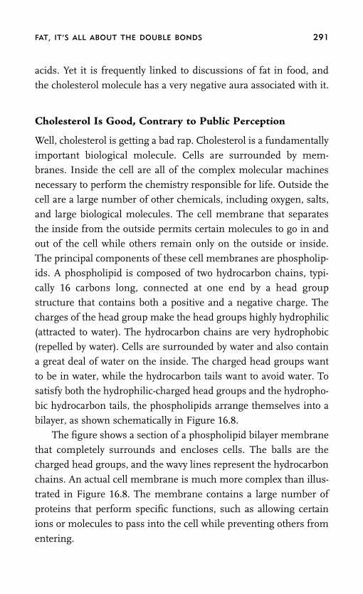
FAT, IT’S ALL ABOUT THE DOUBLE BONDS 291
acids. Yet it is frequently linked to discussions of fat in food, and
the cholesterol molecule has a very negative aura associated with it.
Cholesterol Is Good, Contrary to Public Perception
Well, cholesterol is getting a bad rap. Cholesterol is a fundamentally
important biological molecule. Cells are surrounded by mem-
branes. Inside the cell are all of the complex molecular machines
necessary to perform the chemistry responsible for life. Outside the
cell are a large number of other chemicals, including oxygen, salts,
and large biological molecules. The cell membrane that separates
the inside from the outside permits certain molecules to go in and
out of the cell while others remain only on the outside or inside.
The principal components of these cell membranes are phospholip-
ids. A phospholipid is composed of two hydrocarbon chains, typi-
cally 16 carbons long, connected at one end by a head group
structure that contains both a positive and a negative charge. The
charges of the head group make the head groups highly hydrophilic
(attracted to water). The hydrocarbon chains are very hydrophobic
(repelled by water). Cells are surrounded by water and also contain
a great deal of water on the inside. The charged head groups want
to be in water, while the hydrocarbon tails want to avoid water. To
satisfy both the hydrophilic-charged head groups and the hydropho-
bic hydrocarbon tails, the phospholipids arrange themselves into a
bilayer, as shown schematically in Figure 16.8.
The figure shows a section of a phospholipid bilayer membrane
that completely surrounds and encloses cells. The balls are the
charged head groups, and the wavy lines represent the hydrocarbon
chains. An actual cell membrane is much more complex than illus-
trated in Figure 16.8. The membrane contains a large number of
proteins that perform specific functions, such as allowing certain
ions or molecules to pass into the cell while preventing others from
entering.

292 ABSOLUTELY SMALL
FIGURE 16.8. Schematic of a portion of a phospholipid bilayer with two
cholesterol molecules. The head groups (balls) are charged and want to
be in water. The hydrocarbon tails avoid water by formation of the bi-
layer. The cholesterol hydroxyl is at the water interface.
outside cell - water
inside cell - water
In addition to phospholipids, a major component of cell mem-
branes is cholesterol. Cholesterol comprises as much as 30% of cell
membranes. Figure 16.8 shows a schematic of two cholesterol mol-
ecules replacing two of the phospholipids. Cholesterol is important
because it controls the mechanical properties of the bilayers. With-
out cholesterol, cell membranes would not function. Therefore, cho-
lesterol is essential. The human body produces a great deal of
cholesterol, and only a limited fraction of the necessary cholesterol
is taken in through food. The take-home message is that if you

FAT, IT’S ALL ABOUT THE DOUBLE BONDS 293
could eliminate all of the cholesterol from your body, you would
die.
The Problem with Cholesterol
The problem with cholesterol is not that you take some in when you
eat, but rather how it behaves in the body. Harmful effects on health
from cholesterol are related to fat, but not because cholesterol is a
fat or even because fatty foods may contain cholesterol. Cholesterol
moves through the bloodstream associated with very large biomo-
lecular aggregates called lipoproteins. These are composed of very
large proteins, phospholipids, fats, cholesterol, and other mole-
cules. The lipoproteins can be divided into at least two classes: low-
density lipoproteins (LDL) and high-density lipoproteins (HDL).
They are somewhat egg shaped, with an approximate diameter of
200 A (200 � 10�10 meters). The volume of these particles is ap-
proximately 5,000,000 A3. In contrast, the volume of a cholesterol
molecule is approximately 200 A3. So, an LDL or HDL particle is
about 20,000 times larger than a cholesterol molecule and carries
many cholesterol molecules in the bloodstream. High levels of LDL
relative to HDL are strongly correlated with coronary artery disease
and atherosclerosis. The mechanism is not well understood, but
LDL-carrying cholesterol leads to deleterious deposits in the arter-
ies, while HDL does not. These high levels of LDL, when compared
to HDL (a high LDL to HDL ratio), are produced by saturated fats
and, even worse, trans fats. Saturated fats increase the level of LDL.
Trans fats not only increase LDL levels, but they also decrease HDL
levels, exacerbating the problem. So eating fat does matter, but not
because fatty foods can contain cholesterol. What matters is the na-
ture of the fat we eat. Oils that are high in polyunsaturated fats,
which have not been processed in a manner that produces large
quantities of trans fats, are desirable.

294 ABSOLUTELY SMALL
In Chapter 14, we discussed carbon-carbon single and double
bonds. The types of hybrid atomic orbitals used to form molecular
orbitals were explicated. Quantum theory allows us to understand
the details of bonding and the effects of the nature of bonding on
the shapes of molecules and the strengths of the bonds that hold
atoms together. In this chapter, fats have been used to illustrate
how the seemingly small details of the molecular bonding, such assingle bonds versus double bonds, the number of double bonds,
and cis versus trans structure about a double bond, play fundamen-
tally important roles in biology. The geometry of double bonds may
literally be a life-and-death issue.

17
Greenhouse Gases
IN THIS CHAPTER, we will look at what happens when we burn coal,
oil, or natural gas in power plants to create energy. A major point is
why coal produces so much more of the greenhouse gas, carbon
dioxide, than does oil, which, in turn, produces more than natural
gas per unit of energy. Furthermore, the reason that carbon dioxide
is such an important greenhouse gas is caused by the fundamentalquantum mechanical phenomena of black body radiation and quan-
tized energy levels.
CARBON DIOXIDE FROMBURNING FOSSIL FUELS
Chapter 15 discussed turning wine (ethanol) into vinegar (aceticacid) by adding oxygen to ethanol. When this happens, we say that
ethanol has been oxidized to acetic acid. Oxidation is a chemical
process that can take many forms, but in the case of turning ethanol
into acetic acid, it literally involves the addition of oxygen. The proc-
ess is facilitated by biological enzymes. Hydrocarbons, such as
295

296 ABSOLUTELY SMALL
methane or heating oil, can also be oxidized. However, hydrocar-
bons are very stable molecules. They will only oxidize at high tem-
peratures. Burning fossil fuels is the process of oxidization. It takes
heat to get the process going, but once the oxidation starts, the
breaking of chemical bonds and the formation of new molecules
liberates additional heat (thermal energy) that keeps the process
going.
BURNING METHANE: NATURAL GAS
First, consider what happens when we burn methane (natural gas).
A model of methane is shown in Figure 14.1. Methane (CH4) reacts
with oxygen to give water (H2O) and carbon dioxide (CO2). The reac-
tion can be written as follows.
CH4 � 2O2 V 2H2O � CO2
This chemical equation shows that one molecule of methane will
react with two molecules of oxygen to give two molecules of water
and one molecule of carbon dioxide. The arrow points from the
reactants to the products. This reaction is said to be balanced be-
cause the number of carbon, hydrogen, and oxygen atoms is the
same on both the left and right sides. In a chemical reaction, the
combination of atoms that make up molecules changes, but the
number of each type of atom never changes. Actually, another reac-
tion product is heat. It takes energy to break the C�H bonds of
methane. However, energy is released when the O�H and C�O
bonds are formed to make the products. More usable energy (called
free energy) is released in making the bonds to form water and
carbon dioxide than is used to break the methane bonds. The net
result is that burning methane releases energy that can be used to
do things such as boil water to cook spaghetti or drive a steam tur-
bine to make electricity.

GREENHOUSE GASES 297
WHAT IS A GREENHOUSE GAS?
Methane is a very good fuel, but it produces the greenhouse gas,
CO2. What is a greenhouse gas? A real greenhouse, in which flowers
or tomatoes are grown, is a building that lets in a lot of sunlight.
Today, such buildings may be constructed with large expanses of
plastic that are transparent to sunlight. So the sunlight pours in.
When the sunlight lands on the materials inside the greenhouse,
much of it is absorbed and converted to heat. You probably have
experienced this effect if you have gotten into a car with black or
dark color seats that have been illuminated by the sun through the
windshield. The seats will be very hot. A black steering wheel may,
in fact, even be too hot to touch. As discussed in connection with
Figure 9.1, hot objects give off black body radiation, which is light
with a wide range of colors. The hotter the object, the higher the
frequency of light. The sun is very hot and gives off a great deal of
visible light (see Figure 9.1). A black car seat heated by the sun is
not very hot and gives off low-frequency (long wavelength) black
body radiation. This long wavelength light is in the infrared portion
of the electromagnetic spectrum. It is much lower in energy than
visible light. In a greenhouse, the sunlight heats up the interior, but
the energy that is emitted as infrared black body radiation cannot
pass through plastic or glass. These materials are transparent for
visible light, but not infrared light. Thus, the heat from the sun is
trapped inside the greenhouse, which remains warm even if the
outside temperature is much colder.
Carbon dioxide (water vapor and some other gases) makes the
atmosphere act as a greenhouse for our entire planet. A great deal
of energy falls on the Earth in the form of sunlight. The sunlight
heats the Earth’s surface, and some of the heat energy is reradiated
as infrared black body radiation. The atmosphere is predominantly
composed of gaseous oxygen (O2) and nitrogen (N2). These gases
are transparent in both the visible and infrared parts of the spec-

298 ABSOLUTELY SMALL
trum. If the atmosphere was composed only of oxygen and nitro-
gen, all of the black body radiation emitted by the warm surface of
the Earth would fly right back out into space. The Earth would be
much colder than it is and probably not suitable for human life.
However, the atmosphere contains other gases. It is approximately
78% nitrogen, 21% oxygen, 0.9% argon, and 0.038% carbon dioxide.
In addition, there are traces of other gases and a variable amount ofwater vapor in the air. The concentration of CO2 in the air is very
small but very important. CO2 is transparent to visible light, but
it absorbs infrared light. (The reasons that carbon dioxide absorbs
important wavelengths of infrared light, making it such a serious
greenhouse gas, are described below.) So CO2 lets the sunlight fall
on the Earth’s surface, but it absorbs some of the infrared black
body radiation, preventing it from escaping into space.A good portion of the infrared black body radiation does escape
into space. However, the balance is very delicate. Sunlight is heating
the Earth. Black body infrared radiation emitted into space is cool-
ing the Earth. Absorption of infrared by CO2 in the air reduces the
cooling effect. With too little CO2 in the air, too much heat energy
is radiated into space, and the Earth is too cold. But with too much
CO2 in the air, not enough heat energy is radiated into space, andthe Earth is too hot. The CO2 acts like the glass or plastic windows
in a real greenhouse. It traps heat on the inside, in this case, the
inside of the atmosphere.
Today the concentration of CO2 in the air is 0.038%, or 380 ppm
(parts per million by volume). In 2000, it was 368 ppm. In 1990, it
was 354 ppm. In 1980, it was 336 ppm. In 1970 it was 325 ppm. In
1960 it was 316 ppm. These numbers are from measurementsmade at Mauna Loa, Hawaii. From air trapped in ice, it was found
that in 1832 the CO2 concentration in the air was 284 ppm. There
is a clear trend in the CO2 concentration, and a great deal of scien-
tific work has unmistakably demonstrated that the increase in atmo-
spheric CO2 is produced by human activity. A major contributor to

GREENHOUSE GASES 299
the increase in CO2 in the air is the burning of fossil fuels, althoughother activities, such as clear cutting of rain forests, are also contrib-utors. What happens if the CO2 concentration in the atmospherecontinues to rise? Venus is an extreme example. Its atmosphere ismore than 90% CO2, and its temperature is approximately 900� F(480� C).
BURNING FOSSIL FUELS PRODUCESCARBON DIOXIDE
As we saw in the chemical equation for burning methane (reactingmethane with oxygen), the chemical reaction produces CO2. Burn-ing other fossil fuels also produces CO2. As discussed, heating oilis a mixture of long chain hydrocarbons, ranging from 14 to 20carbons. We will use the 14-carbon molecule, tetradecane, as anexample. Tetradecane is C14H30. The chemical equation for burningtetradecane is
C14H30 � 21.5O2 V 14CO2 � 15H2O.
Tetradecane has 30 H atoms, which make 15 water molecules, eachwith two H atoms. It also has 14 C atoms, which go into the 14carbon dioxide molecules. To make the 14CO2 and 15H2O mole-cules requires 43 oxygen atoms, or 21.5 O2 molecules. That is thereason for the 21.5O2 on the left side of the chemical equation. No-tice that in the chemical equation for burning methane, twice asmany water molecules than carbon dioxide molecules are produced.In burning tetradecane, there are approximately the same numberof water and carbon dioxide molecules produced. This will turn outto be important.
In addition to natural gas (methane) and oil (long chain hydro-carbons), the third common fossil fuel is coal. In its idealized form,coal is pure carbon. This is not actually true, but for right now wewill accept this statement. Then, the chemical equation for burningcoal is

300 ABSOLUTELY SMALL
C � O2 V CO2.
So, in contrast to burning hydrocarbons, burning coal does not pro-
duce any water, just CO2. In burning hydrocarbons, carbon-carbon
and carbon-hydrogen bonds must be broken, which costs energy.Then, carbon-oxygen and oxygen-hydrogen bonds are formed to
make carbon dioxide and water, which produces energy. Coal also
has bonds that must be broken. These are carbon-carbon bonds.
Initially, we will take coal to be graphite, which is pure carbon. We
want to compare the amount of energy produced by burning each
type of fossil fuel with how much of the greenhouse gas, CO2, is
produced. Although graphite is not used as a fuel because it is diffi-cult to ignite, its well-defined chemical structure makes it a useful
example.
Energy Production and the Amount of Carbon Dioxide
First we will look at an idealized picture of energy production from
burning fossil fuels. We ignore the fact that fuels are not pure and
that a good deal of energy is lost in power plants. The actual energyproduction from real fuels will be discussed below. The three chem-
ical equations for burning the fossil fuels are:
CH4 � 2O2 V 2H2O � CO2C14H30 � 21.5O2 V 15H2O � 14CO2
C � O2 V CO2.
In the first and third equations for burning natural gas and coal, a
single CO2 is produced in the reaction. For our model of heating
oil (tetradecane), 14 CO2s are produced. We want to determine theamount of energy produced for one CO2. Using thermodynamics,
it is possible to calculate the maximum usable energy (free energy)
produced by each reaction. We assume that all of the reactions start
at room temperature with methane (a gas), tetradecane (a liquid),
and graphite (a solid). Of course, burning fuel will initially leave the

GREENHOUSE GASES 301
products hot, but we will consider the situation after everything has
cooled to room temperature. For natural gas, we just use the free
energy produced by burning one molecule; for graphite, we use the
energy produced by burning one carbon atom. For tetradecane, we
divide the energy produced by burning one tetradecane by 14 to get
the energy per one carbon dioxide molecule produced.
The results are:
methane (natural gas) 1.4 � 10�18 J free energy generated per
CO2 produced
tetradecane (heating oil) 1.1 � 10�18 J free energy generated per
CO2 produced
graphite (coal) 0.7 � 10�18 J free energy generated per CO2
produced
We see that getting the same amount of energy from coal generates
twice as much carbon dioxide (greenhouse gas) as burning natural
gas. Coal is also a factor of 1.6 worse in terms of greenhouse gas
production for the same amount of energy produced than heating
oil. Heating oil is a factor of 1.3 worse than natural gas.
Burning Real Fossil Fuels
The numbers given here are accurate except for coal. The different
types of coal, that is, anthracite, bituminous, subbituminous, and
lignite (brown coal), produce different amounts of energy per
pound and also have different average carbon contents. Even for the
same type of coal, the energy content and the carbon content vary.
For example, bituminous coal is the most plentiful type in the
United States. Its carbon content ranges from 45% to 86%, and its
energy content varies by approximately �20% around the average.
The calculated value for coal given above using graphite as a model
produces a result corresponding to the middle of the range of en-
ergy content of bituminous coal. Natural gas can have as much as

302 ABSOLUTELY SMALL
20% of the gaseous hydrocarbons ethane (C2H6), propane (C3H8),
and butane (C4H10), in addition to methane (CH4). The mixture
hardly changes the energy content or the energy per CO2 produced
compared to that calculated for pure methane. The same is true of
oil, which is a mixture of long chain liquid hydrocarbons.
Real Numbers for Carbon Dioxide Production fromGenerating Electricity
The energy content of fossil fuels does not take into account power
plant efficiencies, that is, the conversion of the fuel’s energy into
electricity. The efficiencies of power plants, which vary depending
on design and age, are similar regardless of the type of fossil fuel
used. Typically, the efficiency is in the high 30s to 40% range. This
means that only approximately 40% of the fuel’s energy is converted
to electrical energy. In addition, the loss in power transmission
lines is approximately 7%. Thus, if a plant efficiency value of 38%
is combined with the transmission line loss the overall rate of con-
version of fossil fuel energy to usable electricity in our homes is
approximately 35%.
To understand what this means, let’s calculate how much CO2
is produced by a 100-watt lightbulb that burns 24 hours a day for a
year. A watt is a J/s (one joule for one second). A year is 3.2 � 107
seconds. So, our 100-watt lightbulb will consume 3.2 � 109 J in a
year. For natural gas, we said that one molecule of CO2 is produced
for each 1.4 � 10�18 J of chemical energy produced. To get 3.2 �
109 J of energy, we will produce 3.2 � 109/1.4 � 10�18 � 2.3 �
1027 molecules of CO2. This amount is for perfect efficiency. With
35% overall efficiency, 6.4 � 1027 molecules of CO2 will be pro-
duced. 6.02 � 1023 molecules of CO2 weighs 44 g (grams). So, the
weight in grams of the CO2 produced is 5 � 105 g or 1000 pounds.
What we see is that running a 100-watt lightbulb for a year will put
1000 lb of CO2 into the atmosphere using natural gas. If we burn
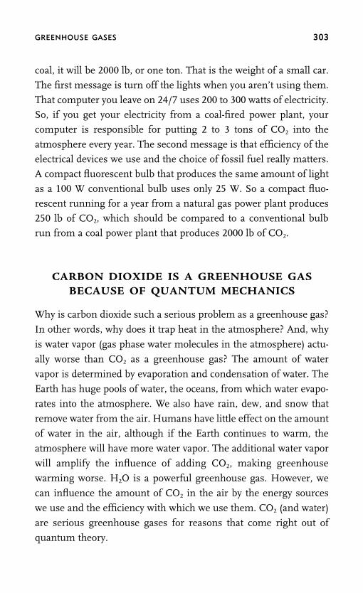
GREENHOUSE GASES 303
coal, it will be 2000 lb, or one ton. That is the weight of a small car.
The first message is turn off the lights when you aren’t using them.
That computer you leave on 24/7 uses 200 to 300 watts of electricity.
So, if you get your electricity from a coal-fired power plant, your
computer is responsible for putting 2 to 3 tons of CO2 into the
atmosphere every year. The second message is that efficiency of the
electrical devices we use and the choice of fossil fuel really matters.
A compact fluorescent bulb that produces the same amount of light
as a 100 W conventional bulb uses only 25 W. So a compact fluo-
rescent running for a year from a natural gas power plant produces
250 lb of CO2, which should be compared to a conventional bulb
run from a coal power plant that produces 2000 lb of CO2.
CARBON DIOXIDE IS A GREENHOUSE GASBECAUSE OF QUANTUM MECHANICS
Why is carbon dioxide such a serious problem as a greenhouse gas?
In other words, why does it trap heat in the atmosphere? And, why
is water vapor (gas phase water molecules in the atmosphere) actu-
ally worse than CO2 as a greenhouse gas? The amount of water
vapor is determined by evaporation and condensation of water. The
Earth has huge pools of water, the oceans, from which water evapo-
rates into the atmosphere. We also have rain, dew, and snow that
remove water from the air. Humans have little effect on the amount
of water in the air, although if the Earth continues to warm, the
atmosphere will have more water vapor. The additional water vapor
will amplify the influence of adding CO2, making greenhouse
warming worse. H2O is a powerful greenhouse gas. However, we
can influence the amount of CO2 in the air by the energy sources
we use and the efficiency with which we use them. CO2 (and water)
are serious greenhouse gases for reasons that come right out of
quantum theory.


304 ABSOLUTELY SMALL
THE EARTH’S BLACK BODY SPECTRUM
In Chapters 4 and 9, we discussed black body radiation. Figure 9.1shows the black body spectrum of the sun, whose surface tempera-
ture is almost 6000� C. The black body emission has a good deal of
its intensity in the visible portion of the spectrum, with a substantial
amount of light being emitted in the ultraviolet and the near infra-
red portions. The colors emitted by a hot object depend on the ob-
ject’s temperature. Hotter objects emit shorter wavelengths. The
Earth is, of course, much colder than the sun. Nonetheless, it is ablack body emitter. Still, the wavelengths it emits are very long (very
low energy photons). Sunlight with the spectrum given in Figure
9.1 falls on the Earth. Some of this light is reflected back into space
by ice and other highly reflecting surface features. However, much
of the light energy is converted into heat, which warms the Earth.
Black body emission by the Earth radiates some of the energy that
comes from the sun back into space.The top portion of Figure 17.1 shows three calculated black
body spectra of the Earth for three temperatures. The three curves
are normalized, that is, their amplitudes adjusted to all have a maxi-
mum value of 1. 15� C (59� F) is the average surface temperature of
the Earth; 27� C (81� F) is the surface temperature in the tropics;
and �16� C (3� F) is the surface temperature in subarctic regions.
While the curves vary somewhat, they are, by and large, very similar.The differences do not matter for discussing the influence of carbon
dioxide.
Absorption of the Earth’s Black Body Radiation
The bottom two spectra in Figure 17.1 (note the frequency scale is
different from the top spectrum) show the atmospheric transmis-
sion of infrared radiation through carbon dioxide and water in the
long wavelength regions. A transmission of 1 means all of the light
passes through the atmosphere. Zero transmission means that
GREENHOUSE GASES 305
FIGURE 17.1. Top: Calculated Earth black body spectra for three temper-
atures (solid curves). The shaded regions show the portions of the spec-
trum that are strongly absorbed by water and carbon dioxide in the
atmosphere. Middle and bottom: spectra of the strong absorption by car-
bon dioxide and water in the range of 0 to 1000 cm�1. Note the scale
difference with the top part of the figure.
0
0.20.4
1.0
0.8
0.6
10008006004002000frequency (cm–1)
tran
smis
sion
100080060040020000
0.20.4
1.0
0.8
0.6
tran
smis
sion carbon dioxide
water
spec
tral
rad
ianc
e (n
orm
aliz
ed)
frequency (cm–1)
81 °F, 27 °C 59 °F, 15 °C 3 °F, –16 °C
water water carbondioxide
0 500 1000 1500 2000 2500 0.0
0.2
0.4
0.6
0.8
1.0

306 ABSOLUTELY SMALL
none of the light passes through the atmosphere. These spectra
differ depending on which region of the Earth they are measured.
The spectra shown are representative. In addition, a good deal of
fine structure (peaks and troughs), particularly in the water spec-
trum, is not shown. The purpose of these curves is to display the
essential features of the infrared absorption by carbon dioxide and
water that are in the intense part of the Earth’s black body spectrum.
These absorptions are indicated by the shaded regions. Water also
has a strong absorption centered around 1750 cm�1, which is also
shaded. The infrared absorption prevents a portion of the Earth’s
black body emission from being radiated into space. Without the
atmospheric absorption, the Earth would be much colder.
The Reason Carbon Dioxide Is So Important
The reason carbon dioxide is so important can be seen by looking
at the shaded regions of the black body spectrum and the absorption
spectra. Water absorbs essentially everything at wavelengths longer
than 500 cm�1. However, the bottom two spectra in Figure 17.1
show that carbon dioxide absorbs strongly in the region where water
absorption is not very strong. The carbon dioxide absorption is very
close to the peak of the Earth’s black body emission spectrum, as
shown in the top part of Figure 17.1, regardless of which Earth
surface temperature is used. Therefore, carbon dioxide strongly ab-
sorbs the Earth’s black body radiation in an important spectral
range where other components of the atmosphere, particularly
water, do not. The carbon dioxide spectrum (middle panel of Figure
17.1) shows that there is close to zero transmission in the middle of
the spectrum, approximately 667 cm�1. However, as the concentra-
tion of CO2 increases, the region of very strong absorption becomes
wider and portions of the spectrum, where a few percent are trans-
mitted, will transmit virtually nothing from the Earth’s atmosphere
into space. The net result is that CO2 absorbs strongly near the peak

GREENHOUSE GASES 307
of the Earth’s black body spectrum where water doesn’t, and an
increase in CO2 in the atmosphere will trap more black body radia-
tion, thereby causing the planet to warm.
Why Carbon Dioxide Absorbs Where It Does
We see that carbon dioxide traps infrared light at the peak of the
Earth’s black body emission and that an increase in CO2 concentra-
tion will have a deleterious effect on the Earth’s temperature. But
why does CO2 absorb infrared light at wavelengths centered at 667
cm�1? In Chapters 8 through 11, we discussed the energy levels of
a particle in a box, of the hydrogen atom, and of all of the other
atoms. In Chapters 12 to 14, we discussed molecular orbitals and
the associated energy levels. All of these discussions concerned the
energy levels associated with electrons. Using the ideas of molecu-
lar orbitals, the nature of bonds that hold atoms together to form
molecules was explicated. What we have not discussed is the mo-
tions of atoms that are bonded together to form molecules.
Figure 12.1 displays the potential energy curve for the hydrogen
molecule, H2. The curve shows the energy at different separations
of the hydrogen atom nuclei. The bond length is the separation
where the energy is a minimum. However, the bond is not rigid. If
we think about the bond using classical mechanics, the bond is a
spring with two masses, the hydrogen atoms, attached at each end
of the spring. A spring can be stretched and compressed. In a classi-
cal system, if you stretch the spring and let go, the masses will
oscillate back and forth with the spring being alternately stretched
and compressed. The masses of a classical oscillator will vibrate
(oscillate) back and forth with a well-defined trajectory. Based on
quantum theory, we should immediately suspect that a quantum
vibration cannot have a well-defined trajectory. Such a trajectory
would mean that we know the positions and moment of the parti-
cles (the atoms) precisely. Such knowledge for absolutely small sys-
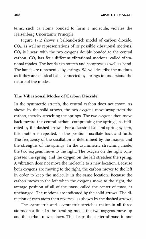
308 ABSOLUTELY SMALL
tems, such as atoms bonded to form a molecule, violates the
Heisenberg Uncertainty Principle.
Figure 17.2 shows a ball-and-stick model of carbon dioxide,
CO2, as well as representations of its possible vibrational motions.
CO2 is linear, with the two oxygens double bonded to the central
carbon. CO2 has four different vibrational motions, called vibra-
tional modes. The bonds can stretch and compress as well as bend.
The bonds are represented by springs. We will describe the motions
as if they are classical balls connected by springs to understand the
nature of the modes.
The Vibrational Modes of Carbon Dioxide
In the symmetric stretch, the central carbon does not move. As
shown by the solid arrows, the two oxygens move away from the
carbon, thereby stretching the springs. The two oxygens then move
back toward the central carbon, compressing the springs, as indi-
cated by the dashed arrows. For a classical ball-and-spring system,
this motion is repeated, so the positions oscillate back and forth.
The frequency of the oscillation is determined by the masses and
the strengths of the springs. In the asymmetric stretching mode,
the two oxygens move to the right. The oxygen on the right com-
presses the spring, and the oxygen on the left stretches the spring.
A vibration does not move the molecule to a new location. Because
both oxygens are moving to the right, the carbon moves to the left
in order to keep the molecule in the same location. Because the
carbon moves to the left when the oxygens move to the right, the
average position of all of the mass, called the center of mass, is
unchanged. The motions are indicated by the solid arrows. The di-
rection of each atom then reverses, as shown by the dashed arrows.
The symmetric and asymmetric stretches maintain all three
atoms on a line. In the bending mode, the two oxygens move up
and the carbon moves down. This keeps the center of mass in one

GREENHOUSE GASES 309
FIGURE 17.2. Top: Ball-and-stick model of carbon dioxide (CO2). Bot-
tom: The three different vibration motions that the molecule can
undergo. There are two bending modes: the one shown and the
equivalent one with the atoms going in and out of the plane of the
page.
symmetric stretch
bend ( 2)
asymmetric stretch

310 ABSOLUTELY SMALL
place. Then the carbon moves up and the two oxygens move down.
In addition to the bending mode shown in Figure 17.2, there is a
second bending mode. The one shown has the motions of the atoms
in the plane of the page. The second bending mode is identical
except the atoms move into and out of the plane of the page.
Quantum Vibrations Have Discreet Energy Levels
In a classical vibrational oscillator made up of balls connected by
springs, the energies the system can have are continuous. Consider
the symmetric stretch. Three balls connected by two perfect springs
are laying on a frictionless table with no air resistance. If you grab
the outer two balls, stretch the springs the same amount, and let
go, the balls will execute the symmetric stretching mode. Because
the spring is perfect, the table is frictionless, and there is no air
resistance (none of which is true in real life), the oscillation will
continue forever. The period or frequency of the oscillation is inde-
pendent of how far you stretch the springs. The period is deter-
mined by the springs’ strengths and the masses. If you stretch the
springs only a little bit, the balls will move slowly. Their average
kinetic energy is small. If you stretch the springs a lot, the balls will
move fast, and the average kinetic energy is large. The energy of the
oscillating ball and spring system is continuous. It only depends on
how much you stretch the springs.
Molecules are not really balls and springs. They are quantum
mechanical systems composed of atoms joined by chemical bonds.
Rather than having a continuous range of energies, the quantum
system has discreet vibrational energy levels. The quantization of
the energy is equivalent to the particle in a box problem discussed
in Chapter 8. Gerhard Herzberg (1904–1999) won the Nobel Prize
in Chemistry in 1971 ‘‘for his contributions to the knowledge of
electronic structure and geometry of molecules, particularly free
radicals.’’ Herzberg’s work on determining the structure of mole-

GREENHOUSE GASES 311
cules was based to a large extent on his explanations for the vibra-
tional spectra of molecules.
The energy of a classical racquetball is continuous, but the en-
ergy of the quantum racquetball (particle in a box) has energy levels
(see Figure 8.6). Figure 17.3 shows a potential curve for a vibrational
mode of a molecule, like the one shown in Figure 12.1, but now the
first several quantized vibrational energy levels are also shown.Again like the particle in a box, the lowest energy level, n � 0, does
not have zero energy.
Energies of Quantized Vibrations
The simplest model for the vibrational energy levels gives the ener-
gies as
E � h�(n � 1/2),
where h is Planck’s constant, � is the vibration frequency, and n is
a quantum number that can take on values, 0, 1, 2, etc. For n � 0,
the energy is 1/2h�. For n � 1, the energy is 3/2h�. So the differ-
ence in energy between the lowest energy level and the first excited
vibration level is h�. In this model, all of the energy levels are
equally spaced with a separation of h�. In real molecules, the energy
levels get somewhat closer together as the quantum number in-creases. For our purposes, we only care about the spacing between
the lowest energy level and first excited energy level.
CO2 Bending Mode Absorbs at the Peak of the Earth’s BlackBody Spectrum
The bottom portion of Figure 17.3 shows the first two vibrational
energy levels. Light will be absorbed at the energy of the separation
of the levels, which is indicated by the dashed arrow. Since the dif-
ference in energy is �E � h� � c h/�, measurement of the light
frequency (�) or the wavelength (�) at which light is absorbed gives

312 ABSOLUTELY SMALL
FIGURE 17.3. Top: A potential energy curve showing the energy as a
function of the bond lengths with the vibrational quantum levels. Only
the first few energy levels are shown. Bottom: The lowest vibrational en-
ergy level (n � 0) and the first excited level (n � 1) for the CO2 bending
modes (Figure 17.2.). This transition (arrow) will absorb the Earth’s
black body radiation (see Figure 17.1).
•••
Ene
rgy
r
�
0
0
n = 1 n = 0
n = 2 n = 4
n = 3
n = 0
n = 1
CO 2 bend E = 667 cm–1
the oscillator frequency. As shown in the figure, �E � 667 cm�1
for the bending modes of carbon dioxide. The two bending modes
have the same frequency because they only differ by the direction
of the bend. (We can write the energy or frequency in wave numbers
[cm�1] by dividing the energy, �E, by c h.) The frequency of light
absorbed by the CO2 bends is almost exactly at the peak of the
Earth’s black body spectrum. It is much easier (takes less energy) to

GREENHOUSE GASES 313
bend a chemical bond than to stretch it. The carbon dioxide sym-
metric and asymmetric stretches are at much higher frequency.
Neither contributes significantly to absorption of the Earth’s black
body radiation.
CO2 GREENHOUSE EFFECTIS QUANTUM MECHANICAL
The important point is that at the most fundamental level, CO2’s
contribution to the greenhouse effect and to global climate change
is inherently quantum mechanical. First, the bonds that are broken
and made in burning natural gas, oil, or coal are determined by the
quantum mechanics that give us molecular orbitals, which control
the bond strengths. The bond strengths determine the amount of
energy that is released per CO2 produced. At an even more funda-mental level, the shape of the black body spectrum emitted by the
Earth is determined by quantum effects. Black body radiation was
discussed in Chapters 4 and 9. Planck’s explanation of the shape of
the black body spectrum and how it changes with the temperature
of a hot object was the first application of quantum theory. The
CO2 absorption centered at 667 cm�1 is a result of the quantized
vibrational energy levels of molecules, a purely quantum effect. TheCO2 bending modes have their quantized n � 0 to n � 1 vibrational
transition at a key frequency in the Earth’s black body spectrum.
While massive power plants, vast numbers of cars, trucks, and
planes, burning of rain forests, etc. produce the greenhouse gas
CO2, it is the quantum interaction between CO2 and the Earth’s
infrared black body radiation that produces the greenhouse effect.
18
Aromatic Molecules
IN CHAPTERS 13 AND 14 we discussed double bonds, and in Chapter 16
we saw that double bonds play a fundamental role in determining
the biological properties of fats. Some of the fat molecules dis-
cussed, the polyunsaturated fats, have several double bonds, but
these double bonds are always separated by a number of single
bonds. For example, Figure 16.5 shows a ball-and-stick model ofDHA, a polyunsaturated fat with six double bonds. As can be seen,
there are two single bonds between each double bond. In this chap-
ter, we will see the wide-ranging impacts of multiple double bonds
that are not separated by several single bonds. Quantum theory
shows that the nature of the bonding found in the molecule ben-
zene and a vast number of other ‘‘aromatic’’ molecules can explain
electrical conductivity in metals, as well as the differences amongmetals, semiconductors, and insulators that will be discussed in
Chapter 19. To understand aromatic molecules and electrical con-
ductivity in metals, it is necessary to discuss the nature of the molec-
ular orbitals that arise when identical atomic orbitals from many
atoms interact to form MOs.
314

AROMATIC MOLECULES 315
BENZENE: THE PROTOTYPICALAROMATIC MOLECULE
Figure 18.1 shows a diagram of benzene, which is composed of six
carbon atoms and six hydrogen atoms. Experiments have deter-
mined that benzene is a perfect hexagon with all of the atoms, car-
bons, and hydrogens in a plane. The angle formed by the bonds
from one carbon to its two nearest neighbors is exactly 120�, and
the angle formed by the bond of a hydrogen to a carbon and that
carbon’s bond to an adjacent carbon is 120�. So the three bonds
made by any carbon have a trigonal geometry, which means they
are formed by the carbon using three sp2 hybrid atomic orbitals on
each carbon. That leaves one unused 2p orbital on each carbon, call
them 2pz orbitals, that point in and out of the plane of the page. We
know that carbon always forms four bonds. Here, a carbon is only
bonded to three other atoms, using up three bonds. The 2pz orbital
must be used to make a � double bond, but where is its location in
the molecule?
FIGURE 18.1. The geometry of benzene,C6H6. Benzene is planar, and it
is a perfect hexagon.
C
CC
C
CC
H
HH
H H
H
120°
120° 120°

316 ABSOLUTELY SMALL
Where Are the Double Bonds?
Figure 18.2 shows two possible double-bonded structures. In both,
each carbon makes four bonds. A carbon makes three � bonds, one
to a hydrogen and one to each of the adjacent two carbons. Each
carbon also participates in a double bond with one adjacent carbon.
The diagrams on the right and left are identical except for the loca-
tions of the double bonds.
Two things are wrong with the bonding in benzene depicted in
Figure 18.2. In the discussion of double bonds in Chapter 14, Table
14.1 shows that the carbon-carbon double bond length is consider-
ably shorter than the single bond length. In ethylene (double bond)
vs. ethane (single bond), the bond lengths are 1.35 A and 1.54 A,
respectively. So if benzene had alternating double and single bonds,
it should have alternating short and long carbon-carbon bonds.
However, experiments demonstrate conclusively that benzene is a
perfect hexagon; all of the carbon-carbon bond lengths are the same.
If we ignore the diagram’s implied unequal bond lengths, the
second problem is the issue of which diagram would be correct, the
FIGURE 18.2. Two possible configurations of double bonds in benzene.
In both, each carbon makes four bonds.
C
CC
C
CC
H
HH
H H
H
C
CC
C
CC
H
HH
H H
H
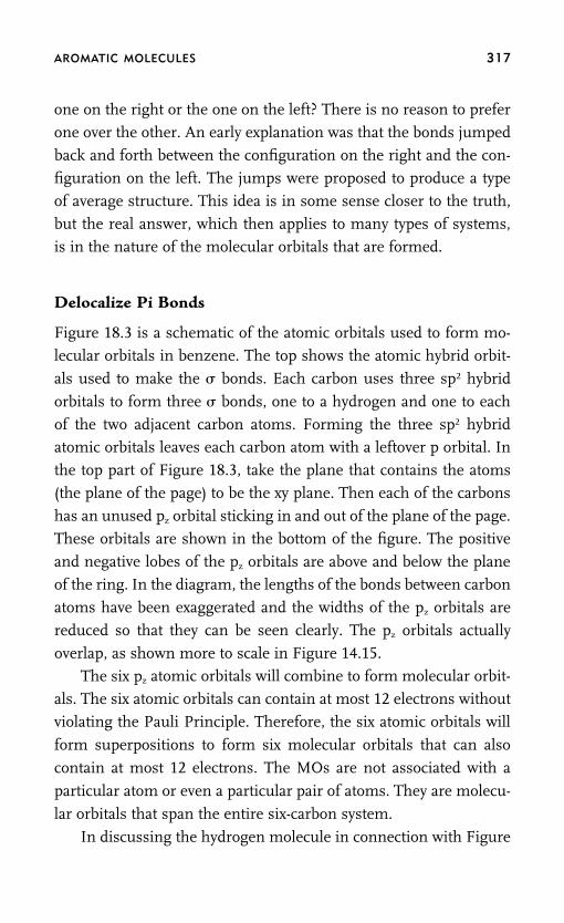
AROMATIC MOLECULES 317
one on the right or the one on the left? There is no reason to prefer
one over the other. An early explanation was that the bonds jumped
back and forth between the configuration on the right and the con-
figuration on the left. The jumps were proposed to produce a type
of average structure. This idea is in some sense closer to the truth,
but the real answer, which then applies to many types of systems,
is in the nature of the molecular orbitals that are formed.
Delocalize Pi Bonds
Figure 18.3 is a schematic of the atomic orbitals used to form mo-
lecular orbitals in benzene. The top shows the atomic hybrid orbit-
als used to make the � bonds. Each carbon uses three sp2 hybrid
orbitals to form three � bonds, one to a hydrogen and one to each
of the two adjacent carbon atoms. Forming the three sp2 hybrid
atomic orbitals leaves each carbon atom with a leftover p orbital. In
the top part of Figure 18.3, take the plane that contains the atoms
(the plane of the page) to be the xy plane. Then each of the carbons
has an unused pz orbital sticking in and out of the plane of the page.
These orbitals are shown in the bottom of the figure. The positive
and negative lobes of the pz orbitals are above and below the plane
of the ring. In the diagram, the lengths of the bonds between carbon
atoms have been exaggerated and the widths of the pz orbitals are
reduced so that they can be seen clearly. The pz orbitals actually
overlap, as shown more to scale in Figure 14.15.
The six pz atomic orbitals will combine to form molecular orbit-
als. The six atomic orbitals can contain at most 12 electrons without
violating the Pauli Principle. Therefore, the six atomic orbitals will
form superpositions to form six molecular orbitals that can also
contain at most 12 electrons. The MOs are not associated with a
particular atom or even a particular pair of atoms. They are molecu-
lar orbitals that span the entire six-carbon system.
In discussing the hydrogen molecule in connection with Figure

318 ABSOLUTELY SMALL
FIGURE 18.3. Top: Benzene � bonding. Each carbon makes three bonds
using three sp2 orbitals that lie in the xy plane. Each carbon has a pz
orbital perpendicular to the plane of the benzene ring. Bottom: The car-
bon pz orbitals have positive and negative lobes that are above and below
the plane of the ring. The bond lengths are exaggerated and the pz lobes
are made small for clarity of presentation. The lobes of adjacent pz orbit-
als overlap.
C
C CC C
CH
H
HH
H
H+ ++
+ ++
---
- -
-
C
C
C
C C
CH
H H
H
H
H
sp2
12.6, we saw that two atomic orbitals combine to form two molecu-
lar orbitals, one bonding MO and one antibonding MO. In Chapter
13, we investigated larger diatomic molecules, such as F2, O2, and
N2. In these atoms, three p orbitals on each atom, six atomic orbitals
total, combined to form six � MOs, three bonding and three anti-
bonding MOs (see Figure 13.5). Some of these diatomic � MOs
were degenerate, that is, they have the same energy.

AROMATIC MOLECULES 319
The Bonding and Antibonding Molecular Orbitals
In benzene, six pz atomic orbitals combine to form three bonding
MOs and three antibonding MOs, as shown in Figure 18.4. The six
carbon 2pz orbitals, one on each carbon atom, have identical energy.
This is indicated by the six closely spaced lines on the left-hand side
of Figure 18.4. These combine to form six MOs with energy levels
shown on the right-hand side of the figure. Three of the MOs haveenergies lower than the pz atomic orbital energy. These are thebonding MOs. Three of the MOs have energies higher than theatomic orbital energy. These are the antibonding MOs. Figure 18.5shows the bonding and antibonding energy levels with the six elec-trons, one from each carbon, placed in the appropriate energy lev-els. We place the electrons in the lowest energy level consistent withthe Pauli Principle. The Pauli Principle (Chapter 11) states that atmost two electrons can be in a single orbital, and they must haveopposite spin states (one up arrow and one down arrow). The firsttwo electrons go into the lowest energy MO. The next two MOs
FIGURE 18.4. Left: Benzene has six carbon atoms, each with a 2pz
orbital. These have identical energy, which is indicated by the six
closely spaced lines. Right: The six pz orbitals combine to form six
� molecular orbitals, three bonding (b) and three antibonding (*)
MOs.
atomic orbitals molecular orbitals
(6) 2p
�
� �
�
�
�z

320 ABSOLUTELY SMALL
FIGURE 18.5. Benzene � molecular orbital energy levels with the six
electrons placed in the appropriate MOs in the lowest possible energy
levels consistent with the Pauli Principle.
antibondingMOs
bondingMOs
have the identical energy indicated by two closely spaced lines. Two
electrons will go into each of these MOs. The three MOs filled by
the six electrons are all � bonding MOs. The � antibonding MOs
are empty.
The Carbon-Carbon Bond Order is 1.5
Figure 18.5 shows that the six carbon pz electrons occupy three �
bonding MOs. Therefore, there are three � bonds shared by six
carbons. These three � bonds are in addition to the � bonds that
connect each carbon to its two nearest carbon neighbors. The net
result is that each carbon has 1.5 bonds to other carbons. The three
� bonds shared by the six carbon atoms contribute a half of a bond
joining adjacent carbons. The bonds between carbon atoms areshorter and stronger than a carbon-carbon single bond, but not as
short or as strong as a full double bond. The � bonding keeps the
molecule rigorously planar. Twisting the ring away from planarity
reduces the overlap of the pz orbitals and raises the energy. Figure
18.6 shows a chemical diagram of benzene. A carbon is represented

AROMATIC MOLECULES 321
FIGURE 18.6. Benzene chemical diagram. A carbon atom is at each ver-
tex, and a hydrogen is at the end of each line from a carbon. The circle
represents the delocalized � molecular orbitals.
by a vertex. A hydrogen atom is at the end of each line that emanatesfrom a carbon. The circle represents the delocalized � electron
system.
Many molecules have carbon rings with delocalized � bonding.
Another example is naphthalene, which is shown in Figure 18.7.
Naphthalene has 10 carbons forming two six-membered rings with
eight hydrogens. The two circles represent the delocalized � molec-
FIGURE 18.7. Naphthalene chemical diagram. Naphthalene has 10 car-
bons and eight hydrogens. The circles represent the delocalized � molecu-
lar orbitals.

322 ABSOLUTELY SMALL
ular orbitals. Like benzene, naphthalene is planar and each carbon
has 1.5 bonds to the adjacent carbons.
THE BENZENE DELOCALIZEDPI MOLECULAR ORBITALS
Benzene, naphthalene, and similar molecules are referred to as aro-matic molecules. They tend to have a sweet smell. Naphthalene is a
mothball, which has a characteristic aromatic smell. Perfumes are
more complex aromatic molecules having a number of benzene-
like rings, as well as other chemical groups replacing the hydrogen
atoms. Small changes in the molecular structure change the aroma,
which is what makes one perfume smell different from another.
In Chapter 8, we discussed the particle in a box problem. Fig-ures 8.4 to 8.6 show the particle in a box wavefunctions and energy
levels. The wavefunction associated with the lowest energy level has
no nodes. The next higher energy state has a wavefunction with one
node, the next higher energy state has a wavefunction with two
nodes, and so forth. A node is a place where the wavefunction goes
to zero, so the probability of finding the electron is zero. The particle
in a box is a one-dimensional problem. A node is a point. In Chapter10, we examined the wavefunctions and the energy levels for a hy-
drogen atom. Figures 10.2 to 10.6 show representations of the wave-
functions for the 1s, 2s, and 3s hydrogen atom states. The hydrogen
atom wavefunctions are three-dimensional. The lowest energy state
(1s) has no nodes, the next higher energy state (2s) has a wavefunc-
tion with one node. The next higher energy state (3s) has two nodes.
These nodes are three dimensional surfaces on which there is zeroprobability of finding the electron.
The benzene � MOs also have an increasing number of nodes
as the energy is increased. Figure 18.8 shows schematics of the
benzene � MOs. The shaded areas are the regions of high electron
density (high probability of finding electrons) for the � MOs.
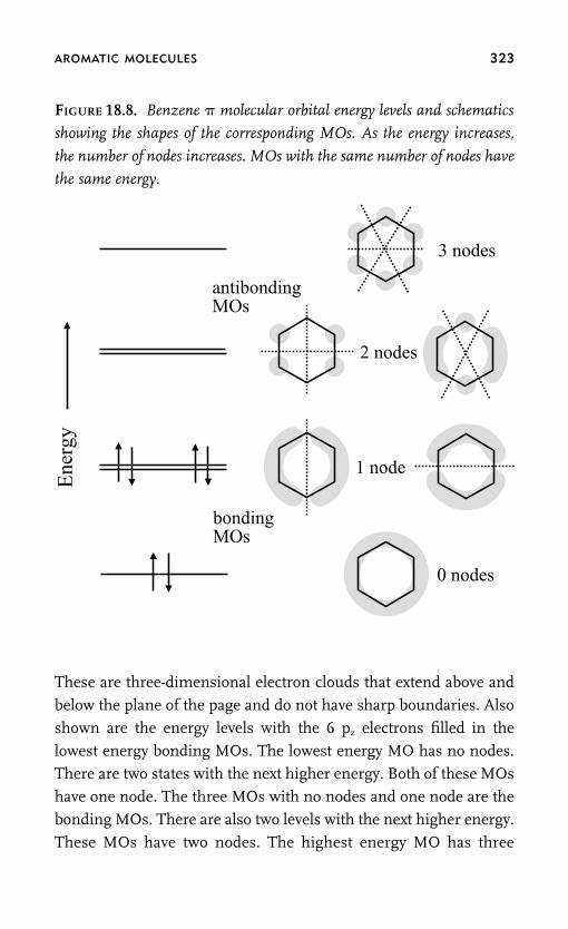
AROMATIC MOLECULES 323
FIGURE 18.8. Benzene � molecular orbital energy levels and schematics
showing the shapes of the corresponding MOs. As the energy increases,
the number of nodes increases. MOs with the same number of nodes have
the same energy.
antibondingMOs
bondingMOs
Ene
rgy
3 nodes
2 nodes
1 node
0 nodes
These are three-dimensional electron clouds that extend above and
below the plane of the page and do not have sharp boundaries. Also
shown are the energy levels with the 6 pz electrons filled in thelowest energy bonding MOs. The lowest energy MO has no nodes.
There are two states with the next higher energy. Both of these MOs
have one node. The three MOs with no nodes and one node are the
bonding MOs. There are also two levels with the next higher energy.
These MOs have two nodes. The highest energy MO has three

324 ABSOLUTELY SMALL
nodes. The three MOs having two and three nodes are the antibond-
ing MOs.
Comparing the schematics of the lowest energy MO with the
highest energy MO in Figure 18.8, it can be seen clearly why the
former is a bonding MO and the latter is an antibonding MO. The
lowest bonding MO has electron density between all of the carbons.
The highest antibonding MO has nodes between all of the carbons,
so electrons in this MO would not join the carbons together. The
pair of bonding MOs, although higher in energy than the lowest
energy bonding MO, results in bonding among the carbon atoms.
Each of these MOs has one node. The one on the left puts electron
density between a pair of carbons on the left and right. The MO on
the right puts electron density between three carbon atoms on the
top and three on the bottom. In spite of the nodes, these MOs com-
bine with the lowest energy MO to produce the three � bonds that
are shared by the six carbons. The two degenerate antibonding MOs
have two nodes each. The one on the left clearly does not contribute
to bonding because it does not place electron density between any
of the carbons. The one on the right puts electron density between
two pairs of carbons, but when combined with the one on the right,
it does not produce net bonding.
Light Absorption by Aromatic Molecules
Quantum theory can calculate the molecular orbitals of aromatic
molecules, as well as their shapes and sizes. There are many ways
to test the quantum calculations by comparison to experiments.
One of the most useful is to employ optical spectroscopy to measure
the wavelengths (colors) of light absorbed by a molecule. We will
use naphthalene as an example.
Figure 18.7 shows a diagram of naphthalene, with its 10 carbon
atoms. Each carbon atom will contribute one pz orbital with one
electron to form the delocalized � electron system. The other three
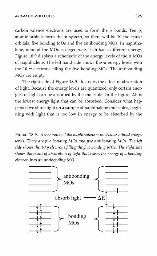
AROMATIC MOLECULES 325
carbon valence electrons are used to form the � bonds. Ten pz
atomic orbitals form the � system, so there will be 10 molecular
orbitals, five bonding MOs and five antibonding MOs. In naphtha-
lene, none of the MOs is degenerate; each has a different energy.
Figure 18.9 displays a schematic of the energy levels of the � MOs
of naphthalene. The left-hand side shows the � energy levels with
the 10 � electrons filling the five bonding MOs. The antibonding
MOs are empty.
The right side of Figure 18.9 illustrates the effect of absorption
of light. Because the energy levels are quantized, only certain ener-
gies of light can be absorbed by the molecule. In the figure, �E is
the lowest energy light that can be absorbed. Consider what hap-
pens if we shine light on a sample of naphthalene molecules, begin-
ning with light that is too low in energy to be absorbed by the
FIGURE 18.9. A schematic of the naphthalene � molecular orbital energy
levels. There are five bonding MOs and five antibonding MOs. The left
side shows the 10 p electrons filling the five bonding MOs. The right side
shows the result of absorption of light that raises the energy of a bonding
electron into an antibonding MO.
bondingMOs
antibondingMOs
absorb light E�

326 ABSOLUTELY SMALL
molecules. The energy of the light is E � h�, where h is Planck’s
constant and � is the frequency. So initially, �E � h�; the energy
separation between the highest occupied molecular orbital (HOMO)
and the lowest unoccupied molecular orbital (LUMO) is greater
than the energy of the photons that are impinging on the sample.
As a result, they pass through the sample without being absorbed.
Now, we start changing the energy of the light to higher energy (red
to blue). When h� � �E, light is absorbed, which is detected by a
decrease in the amount of light that passes through the sample. An
electron is excited from the HOMO to the LUMO. This excitation is
shown on the right side of Figure 18.9, which has one electron in
the HOMO and one electron in the LUMO. In the left-hand side of
Figure 18.9, there are two electrons in the HOMO and none in the
LUMO.
The transition from the HOMO to the LUMO is the lowest en-
ergy transition. As drawn, the bonding MOs are closer together than
the separation between the HOMO and the LUMO. However, an
electron cannot be excited from one filled bonding MO to another
filled bonding MO. If we try to take an electron from one bonding
MO and put it into another bonding MO, the result would be an
MO with three electrons in it. Three electrons in an MO violates the
Pauli Exclusion Principle. Then in our optical absorption experi-
ment, as the light color is scanned from red to blue (low energy to
high energy), the first color (wavelength) that is absorbed corre-
sponds to the energy �E. �E can be calculated using quantum me-
chanics. �E depends on the structure of the molecule and the
interactions of the atomic orbitals that give rise to the molecular
orbitals. The quantum calculations can be tested further by compari-
son to the wavelengths at which absorption of higher energy light
takes place as the light is scanned further and further to the blue.
This second absorption occurs because light can take an electron
from the HOMO to one energy level above the LUMO. Another

AROMATIC MOLECULES 327
absorption at even higher energy will occur by exciting an electron
from the HOMO to two levels above the LUMO, and so forth.
NAPHTHALENE TREATED AS APARTICLE IN A BOX PROBLEM
Using modern quantum theory and computers, the structure of
naphthalene can be calculated with great accuracy. The theory will
give the bond lengths and bond angles. For example, the bondlengths can be calculated to 0.001 nm, that is, a thousandth of a
nanometer. The calculations also yield the frequencies at which
light is absorbed with substantial accuracy. The calculations use the
masses, number of electrons, and charges of the nuclei. The calcula-
tions will include both the � and � bonding. As we have discussed,
the � electrons are not localized on one or two carbon centers, but
rather are delocalized over the entire carbon framework of the mole-cule. The lowest energy absorption of naphthalene, the HOMO to
LUMO absorption, occurs at 320 nm, which is in the ultraviolet
portion of the optical spectrum.
We can do a very crude calculation by pretending that the �
electrons are particles in a box. In Chapter 8, we discussed the parti-
cle in a box in great detail. If we take the HOMO to LUMO transi-
tion to be a transition of an electron in a box from the n � 1 to n� 2 levels (see Figure 8.7), we can use the formulas derived just
below Figure 8.7. For this transition we found that
�E�3h2
8mL2
where h is Planck’s constant, m is the mass of the electron, and Lis the length of the box. Here we will take L to be 0.51 nm, the
distance across the carbon framework of naphthalene. Then,
�E�3(6.6�10�34)2
8(9.1�10�31)(0.8�10�9)2�6.9�10�19 J.

328 ABSOLUTELY SMALL
Converting this energy to a frequency by dividing by h gives � �
1.04 � 1015 Hz. Then the wavelength of the light that will be ab-
sorbed is � � 2.87 � 10�7 m � 287 nm. This wavelength is further
in the ultraviolet than the true absorption, but not that far from the
observed value.
The particle in a box calculation shows that if a particle with the
mass of an electron is confined to a box the size of naphthalene,the first absorption will be in the ultraviolet range. The reasonable
accuracy of the particle in a box calculation for naphthalene is some-
what fortuitous. Even if we wanted to model naphthalene as a parti-
cle in a box, it should be a two- or three-dimensional box, not a one-
dimensional box. Such calculations produce results with significant
errors. However, an accurate quantum theory calculation will yield
the molecular structure and much more accurate frequencies forabsorption of light. In addition, if, for example, a hydrogen is re-
placed by a fluorine, quantum theory will accurately predict how
much the frequency of light absorption of fluoronaphthalene is
changed from that of naphthalene.

19
Metals, Insulators,
and Semiconductors
FIGURE 19.1 IS A SCHEMATIC DIAGRAM of a battery connected to a metal
rod. We will discuss sodium metal below as an example, but the rod
could be any metal. The positive end of the battery pulls electrons
from the metal rod. Electrons flow out of the rod into the battery.
FIGURE 19.1. A metal rod of sodium, for example, is connected by wires
to a battery. Negatively charged electrons are pulled from the metal rod
to the positive side of the battery. Electrons flow from the negative side of
the battery back into the metal rod.
e- e-
+-batterywire
metal rod
329

330 ABSOLUTELY SMALL
However, to keep the rod from developing a positive charge that
would pull back on the electrons and stop the flow, the rod must be
connected to the negative side of the battery.
Electrons flow from the negative side of the battery into the rod,
keeping the rod neutral, that is, the rod does not develop an electri-
cal charge. Instead of a rod, the electrons could flow through the
filament of a lightbulb in a flashlight. The flow of electrons throughthe filament causes it to get very hot and produce black body radia-
tion in the visible part of the spectrum.
METALS
Delocalize Molecular Orbital for a Metal
How can electrons move through a piece of metal? What is thedifference between a metal and an insulator? What is a semiconduc-
tor? Why does a metal get hot when electrons flow through it? What
is superconductivity? To answer the first three questions, we will
extend our discussion of the types of delocalized molecular orbitals
found in aromatic molecules such as benzene and naphthalene (see
Chapter 18) to the MOs of a macroscopic piece of metal and other
materials. To answer the last two questions, we will expand the dis-cussion to the effect of the thermal vibrations of the atoms that
make up a piece of metal on electron motion in a metal.
In Chapter 10 on the hydrogen molecule, we saw two hydrogen
atomic orbitals combine to form two molecular orbitals, one bond-
ing and one antibonding. In benzene, we saw that six pz atomic
orbitals, one from each carbon, combined to form six MOs, three
bonding MOs and three antibonding MOs. For naphthalene, 10 pz
atomic orbitals combined to form 10 MOs, five bonding and five
antibonding. In each case, the MOs span the entire molecule. In
Chapter 11 on the Periodic Table of Elements, we said that sodium,
Na, is a metal because it has one electron, the 3s, past the neon
filled shell configuration. Na can readily give up an electron to form

METALS, INSULATORS, AND SEMICONDUCTORS 331
salts, such as table salt, NaCl. In water NaCl dissolves to become
Na� and Cl�. We said that Na as a solid was a metal and conducted
electricity. Now we are in a position to see why.
First consider the 3s orbitals of two sodium atoms that are next
to each other and interacting. For sodium, the 3s electron is the
valence electron, which will participate in bonding. The top portion
of Figure 19.2 shows the energy levels of the two 3s atomic orbitalscombining to form MOs. One of the MOs has lower energy than
the atomic orbitals. It is the bonding MO. The other MO has higher
energy; it is the antibonding MO. The middle shows that three
atomic orbitals will form three MOs. The bottom illustrates the situ-
ation for six interacting sodium atoms. The six 3s atomic orbitals
combine to form six MOs, three bonding and three antibonding.
Each Na has one 3s electron, which it will contribute to fill the
MOs. For the system with six sodium atoms, there will be six elec-
FIGURE 19.2. Top: Two sodium 3s atomic orbitals interact to produce
two molecular orbitals, one lower in energy (bonding) and one higher in
energy (antibonding). Middle: Three 3s atomic orbitals interact to form
three MOs. Bottom: Six 3s atomic orbitals interact to form six MOs.
(3) 3s
(6) 3s
3s 3s

332 ABSOLUTELY SMALL
trons to fill the MOs. Each MO can be occupied by two electrons
with opposite spins (one up arrow and one down arrow). Therefore,
the three lowest energy MOs, which are the bonding MOs, will be
filled by the six electrons. The three higher energy MOs are empty.
Now we must consider what happens when we have a very large
number of interacting sodium atoms. Consider a metal rod com-
posed of sodium atoms that is 10 cm long and 1 mm in diameter,
such as that in Figure 19.1. For the dimensions given, the rod con-
tains N � 2 � 1021 Na atoms, where N is the number of atoms.
This number is two billion trillion atoms. The two billion trillion 3s
atomic orbitals combine to form two billion trillion molecular orbit-
als. Like the MOs of benzene or naphthalene, the MOs of the so-
dium rod should be thought of as spanning the entire system, that
is, the entire piece of metal.
A Piece of Metal Has a Vast Number of MO Energy LevelsCalled a Band
Figure 19.3 illustrates the energy levels of this system. Each of the
N sodium atoms has an electron in a 3s atomic orbital. In the ab-
sence of interactions between the atoms, all of these atomic orbitals
have the same energy. In the figure, this is represented by the col-
lection of closely spaced lines on the left-hand side. To show that
there are many atomic levels, the lines have been spread out, but
they all have the same energy. When the atoms interact, the N
atomic orbitals form N MOs. As we have seen previously for mole-
cules, the MOs have different energies. Some of the MOs have
lower energies than the atomic orbital energy and some have higher
energy. This is represented on the right side of the figure by the
spread-out but closely spaced lines. The MO energy levels in Figure
19.3 are equivalent to those shown in Figures 18.8, 18.9, and 19.2,
except that there are vastly more energy levels, which are much
more closely spaced. These are referred to as a band of states.

METALS, INSULATORS, AND SEMICONDUCTORS 333
FIGURE 19.3. In a piece of sodium metal, there are N atoms. Each has
an electron in a 3s orbital, represented by the closely spaced lines on the
left. These all have the same energy. The N 3s atomic orbitals interact to
form N molecular orbitals with energy levels shown on the right. The MO
energy levels are so close together that the energy is effectively a continu-
ous band of states. The Fermi level marks the highest occupied molecular
orbital.
N 3s orbitals Fermi level
band of states
Quantum theory shows that the width of the band of states, that
is, the difference in energy between the highest energy MO and the
lowest energy MO, is only a few times the energy splitting of the
MOs that arise from a pair of interacting sodium atoms (see Figure
19.2, top). Then in our example of two billion trillion Na atoms,
there are this many energy levels in a relatively narrow range ofenergy. The result is that the energy levels are so closely spaced that
the energy is effectively continuous within the band.
Putting in the Electrons
There are N sodium atoms, each with a single 3s electron. We need
to take these N electrons and put them in the appropriate MOs, as
we did with small molecules in Chapters 12 and 13 and as shown

334 ABSOLUTELY SMALL
in Figures 18.8 and 18.9. These sodium metal delocalized MOs are
orbitals like any others, so we must obey the three rules for putting
in the electrons discussed in Chapter 11. They are lowest energy
first, no more than two electrons in an orbital that must have paired
spins (Pauli Exclusion Principle), and don’t pair spins unless neces-
sary (Hund’s Rule). Figure 19.3 illustrates putting in the electrons.
The first electron goes in the lowest energy level. The next electron
goes into the same level with the opposite spin, that is, one up arrow
and one down arrow. The third electron can’t go into the lowest
energy level because that would violate the Pauli Principle. So, it
goes into the level one up from the lowest. The fourth electron goes
into this same level with paired spins. This will continue until all N
electrons are in MOs.
The Fermi Level
There are N MO energy levels and N electrons. But two electrons
can go in each level. Therefore, only the bottom half of the energy
band of levels will be filled. This is like benzene (Figure 18.8) and
naphthalene (Figure 18.9), which also only have the bottom half of
their MOs filled. The energy of the highest filled orbital is called the
Fermi level, for Enrico Fermi (1901–1954). Fermi was a physicist
who worked in many areas of science including the theory of solids,
such as metals, and the theory of nuclear reactions. His work con-
tributed to the development of nuclear energy. He won the Nobel
Prize in Physics in 1938 ‘‘for his demonstrations of the existence of
new radioactive elements produced by neutron irradiation, and for
his related discovery of nuclear reactions brought about by slow
neutrons.’’ As we will see, the Fermi level is very important.
The Fermi level is the level of the highest filled MO at the abso-
lute zero of temperature. This temperature is 0� K, where K is the
Kelvin unit of temperature. One degree K is the same as one degree
C (centigrade) except the scale begins at the absolute zero of temper-
METALS, INSULATORS, AND SEMICONDUCTORS 335
ature. 0� K is �273� C or �459� F. We have briefly discussed how
heat in systems of molecules, such as water, causes the molecules
to jiggle around. In Chapter 15, it was pointed out that the thermal
motions of water were responsible for the breaking of hydrogen
bonds between water molecules. As temperature is decreased, there
is less and less heat (thermal energy) and the motions of atoms and
molecules decrease. The absolute zero of temperature, 0� K, is the
temperature at which there is no heat to cause atoms and molecules
to move. The Fermi level is actually defined to be the energy of the
highest filled MO at 0� K.
How Electrons Move Through Metal
As shown in Figure 19.1, electrons enter one side of the metal rod
and leave the other. This is possible because the electrons are in
delocalized MOs that span the entire piece of metal. However,
quantum theory shows that if all of the electrons occupy only the
MOs below the Fermi level, the electrons will not move in a particu-
lar direction. Real metals are three dimensional, but for this discus-
sion let’s consider only one dimension at a time. In our metal rod,
when it is not connected to the battery, the electrons in the MOs
are, nonetheless, constantly moving. Although the electrons are de-
scribed in terms of quantum mechanical wavefunctions, the elec-
trons have kinetic energy. Therefore, it is possible to calculate an
electron velocity. The electrons in some MOs can be thought of as
moving to the right. There are corresponding MOs of identical en-
ergy with electrons moving to the left. With all of the MOs filled, as
shown in Figure 19.3, there will be no net electron current because
there are an equal number of electrons moving to the right and to
the left. In three dimensions, for any direction you pick, there will
be equal probability of electrons moving in that direction and in the
exact opposite direction.
However, when the metal rod in Figure 19.1 is connected to a

336 ABSOLUTELY SMALL
battery, things change. One end of the rod is connected to the posi-
tive side of the battery and the other end is connected to the negative
end of the battery. The connection to the battery changes what the
electrons feel. Without the battery, the electrons feel the positive
charges of the sodium nuclei and the negative charges of other elec-
trons. Any one electron in the middle of the rod sees no difference
between right and left. But with the battery there is an additional
influence, the electric field produced across the metal rod by the
battery. The electrons are attracted to the positive end and repelled
from the negative end. The effect is to modify the system with the
result that some electrons are in levels above the Fermi level that
existed without the battery (see Figure 19.4). The electron states of
the system are changed such that there are more electrons moving
in the direction toward the positive end of the metal rod than toward
the negative end.
FIGURE 19.4. Schematic of the sodium metal 3s band of levels as shown
in Figure 19.3, but now with the influence of being connected to the
battery. The effect is to put some electrons above the no battery Fermi
level, taking them from filled MOs to empty MOs. These electrons are
represented by the arrows above the Fermi level.
N 3s orbitals Fermi level
band of states

METALS, INSULATORS, AND SEMICONDUCTORS 337
Quantum theory shows that it is necessary to have electrons
above the Fermi level for electron conduction to occur. Because
there are only infinitesimal differences in energy between the levels,
even a very low voltage applied to the rod, which produces a tiny
electric field, is sufficient to put some electrons above the Fermi
level. The result is an electrical current flowing throw the metal
rod. Electrons leave the positive end of the rod and are replaced byelectrons entering from the negative end. For a bigger electric field
(higher voltage), more electrons will be above the zero field Fermi
level, and the electrical current is bigger. The detailed quantum the-
ory of electrical conductivity in metals says that current will flow
when an electric field is applied even at absolute zero temperature.
Heat is not required for a metal to conduct. We will see below that
this is not the case for semiconductors, and also, that heat, which ispresent at all temperatures above 0� K, actually interferes with elec-
trical conductivity in metals.
INSULATORS
Insulators Do Not Conduct Electricity Because theBand Is Filled
Metals conduct electricity easily even at 0� K because the electrons
only fill part of the band of states, as shown in Figure 19.3 and 19.4.
A very small electric field (voltage) will put electrons above the
Fermi level. An insulator is a material, such as glass or plastic, that
does not conduct electricity at any temperature. A schematic illus-
tration of the band structure of an insulator is shown in Figure 19.5.
In sodium metal, the 3s electrons are the valence electrons. Thevalence band is only half filled. In an insulator, like quartz (SiO2,
silicon dioxide), which is very similar to glass, sharing of the elec-
trons completes the shell of electrons. The interactions in a quartz
crystal produce a band of states, with delocalized MOs, like in a
metal. However, the valence band is completely filled. There are two

338 ABSOLUTELY SMALL
FIGURE 19.5. Schematic of the band structure of an insulator. There is
a filled band, with two electrons in each MO. At much higher energy,
there is an empty band.
filled band
Fermi level
empty band
bandgap
electrons in each MO because there are N MOs but 2N electrons.
So, all of the MOs have two electrons, from the lowest energy level
to the highest energy level in the band. The filled band is shown in
Figure 19.5 by the presence of arrows from the bottom of the band
METALS, INSULATORS, AND SEMICONDUCTORS 339
to the top of the band. This filled band should be compared to the
half-filled band of Na metal shown in Figure 19.3.
The Band Gap Is Large in Insulators
There are empty atomic orbitals at much higher energy, and these
form MOs. However, there are no electrons to put in these MOs.
Therefore, the next higher energy band is completely empty. The
difference in energy between the top of the filled band and the bot-
tom of the unfilled band is called the band gap. The Fermi level is
at the top of the filled band.
As discussed qualitatively above and shown in detail by quan-
tum theory, conductivity requires electrons in MOs with energies
above the Fermi level. When an electric field is applied across the
material (connected to a battery or other source of voltage), the na-
ture of the delocalized states shifts. In a metal, because the band
is only half filled and the energy levels are only separated by an
infinitesimal amount, an applied electric field will result in a change
such that some electrons are above the zero field Fermi level, and
electrons flow through the metal. In an insulator, the next level
above the Fermi level is in the empty band. The band gap is large,
and the application of an electric field cannot change the system
enough to put electrons into the empty band. Therefore, application
of an electric field to an insulator is insufficient to produce conduc-
tivity, in contrast to a metal.
Another possibility is that thermal energy could excite electrons
from the filled band to the empty band. An insulator has the prop-
erty that the band gap energy is much greater than the thermal
energy. As the temperature is increased, the amount of thermal
energy increases. But an insulator has a band gap that is so large
that the insulating material will be destroyed at temperatures that
are still insufficient to thermally excite electrons from the filled
band to the empty band. The net result is that application of an

340 ABSOLUTELY SMALL
electric field cannot modify the states in a way to produce conductiv-
ity and thermal excitation of electrons cannot occur. Therefore, in-
sulators do not conduct electricity.
SEMICONDUCTORS
In a Semiconductor the Band Gap Is Small
A semiconductor is like an insulator, but with a small band gap. A
schematic of the band structure of a semiconductor is shown in
Figure 19.6. In a semiconductor, such as silicon (Si), there are
enough electrons to fill the valence band completely. At 0� K, where
there is no thermal energy to excite electrons, all of the electrons
are paired in the valence band. The Fermi level is at the top of the
filled valence band. Therefore, silicon is an insulator at 0� K. How-ever, in silicon and other semiconductors, the band gap is small. At
room temperature, there is sufficient thermal energy to excite some
electrons above the Fermi level into the next band. The thermal
energy is contained in the motions of the atoms in a piece of semi-
conductor. The thermal excitation of electrons above the Fermi level
into the next band is illustrated in Figure 19.6. The electrons that
have been excited from filled MOs of the valence band to emptyMOs of the conduction band are represented in the figure by arrows
above the Fermi level. Because there are electrons above the Fermi
level, a piece of semiconductor like silicon can conduct electricity.
The electrons in the conduction band are called the conduction elec-
trons.
Semiconductors do not conduct electricity as well as metals be-
cause they have far fewer conduction electrons. In a metal, there isno band gap. Large numbers of electrons are easily promoted above
the Fermi level. In a semiconductor, there is a band gap, but it is
small enough that thermal energy can excite some electrons above
the Fermi level into the conduction band. As the temperature of a
semiconductor is reduced, there are fewer and fewer conduction

METALS, INSULATORS, AND SEMICONDUCTORS 341
FIGURE 19.6. Schematic of the band structure of a semiconductor. The
valence band is essentially filled. The gap in energy to the next band is
relatively small. Some electrons are thermally excited above the Fermi
level into the conduction band.
valenceband
Fermi level
conductionband
smallbandgap
electrons to carry electrical current. At sufficiently low temperature,semiconductors become insulators. The only difference between asemiconductor and an insulator is the size of the band gap. Yourcomputer chips, which are composed mainly of silicon semiconduc-tors, will not work if they are sufficiently cold. The computers andelectronics on a satellite must be kept warm or they will cease tofunction.
342 ABSOLUTELY SMALL
Thermal Energy Affects Electrical Conduction in Metals
Thermal energy is necessary in semiconductors to generate conduc-
tion electrons. Thermal energy also strongly influences electrical
conduction in metals, although thermal energy is not necessary to
generate the conduction electrons. In a piece of metal wire con-
nected to a battery, there are electrons moving toward the positive
end. As electrons leave the wire, they are replenished by electrons
entering from the negative side of the battery. Current (electrons)
flowing through a piece of wire will cause its temperature to rise.The heating elements in an electric stove or an electric space heater
get very hot from a large current flowing through them. They get so
hot that they glow red. The red color is black body radiation from
the hot metal. We have said that electrons can readily flow through
a piece of metal because the electrons are in delocalized MOs that
span the metal. It only requires an electric field (connection to a
battery or other voltage source) to get them moving in a particulardirection. So the question is why does the flow of electrons cause
the metal to heat up?
The electrons in a metal should be thought of as wave packets
that are more or less localized. We discussed wave packets in Chap-
ter 6 in connection with the Heisenberg Uncertainty Principle. The
electron wave packets in a metal are formed from superpositions of
the delocalized electronic MO wavefunctions in a manner analo-gous to photon wave packets or electron wave packets in a vacuum
that are superpositions of the delocalized momentum states. Elec-
trons are negatively charged so an electron wave packet carries a
negative charge. The electron is accelerated toward the positive end.
The acceleration gives the electron increased kinetic energy.
Vibrations of a Solid Are Phonons
In Chapter 17, we briefly discussed the quantized vibrations of mol-
ecules in connection with the greenhouse gas, carbon dioxide. A
METALS, INSULATORS, AND SEMICONDUCTORS 343
piece of metal, which is made up of atoms, also has quantized vibra-
tions. The atoms in a metal crystal lattice can jiggle around in their
positions. Although they jiggle, an atom remains in the same spot
on average. The motion of each atom is connected to the motions
of the other atoms in the same manner that the motions of the
atoms of a CO2 molecule are connected to each other (see Figure
17.2). CO2 has several distinct vibrations, symmetric and antisym-
metric stretches, and two bending modes. These three different
types of modes have vibrational energies (frequencies) that are very
different from each other.
In a metal crystal lattice, each atom can move in all three dimen-
sions. For N atoms, there are 3N lattice vibrations, where again, N
is the number of atoms in the piece of metal. For any finite size
piece of metal, this huge number of vibrations results in a band of
vibrations rather than several discreet frequencies. At low tempera-
ture, only the lowest energy part of the band of vibrations is ther-
mally excited. At higher temperature more lattice vibrations are
excited and higher energy vibrations are excited. The excited vibra-
tions have kinetic energy. The energy of the excited vibrations is
what we think of as heat.
The quantized vibrations of a lattice are called phonons. This
name came about because phonons in certain fundamental quan-
tum theory properties bear some resemblance to photons. Each
phonon is a delocalized vibrational wave that spans the entire crystal
lattice. The lattice waves can form more or less localized wave pack-
ets through the superposition of a range of wavelengths of lattice
waves. The more or less localized phonon wave packet is completely
analogous to the photon and electron wave packets mentioned just
above and discussed in Chapter 6. The phonons are moving wave
packets of mechanical thermal energy. The phonon wave packet can
be thought of as a moving region of relatively localized jiggling of
the atoms.

344 ABSOLUTELY SMALL
Electron Wave Packets and Phonon Wave Packets Scatter
An electron wave packet that is being accelerated toward the positive
direction can interact with a phonon. The phonon causes the posi-
tively charged atomic nuclei to move. The negatively charged elec-
tron is influenced by the moving positive charges. The interaction
of the electron and phonon is called a scattering event and is shown
schematically in Figure 19.7. The electron and phonon wave packets
are propagating in certain directions. The electron is being acceler-
ated by the electric field when it ‘‘collides’’ with a phonon. Following
FIGURE 19.7. Cartoon of an electron-phonon scattering event. The inter-
action of the electron and phonon causes the directions of the wave packet
motions to change.
electron wave packet
phononwave packet
scatteringevent

METALS, INSULATORS, AND SEMICONDUCTORS 345
the scattering event, in general, both wave packets will move in new
directions. The electron will again be accelerated by the electric field
toward positive. After some time, it will again encounter a phonon,
and scatter. Each time the electron scatters, it gives up some of its
kinetic energy to a phonon that it got from being accelerated by the
electric field (voltage source).
The scattering events do two things. First, they prevent the elec-
trons from moving directly to the positive battery connection. Sec-
ond, the scattering events add kinetic energy to the phonons. The
electron loses energy, and the phonon gains it. The electron-phonon
scattering reduces the electrical conductivity of metals because the
electrons keep getting bumped, which causes them to move in dif-
ferent directions as they are trying to move to the electrically posi-
tive end of the wire. This is called electrical resistance. At very low
temperature, there are few phonons, so the electrons can move a
long way between scattering events. This makes it easier for the
electrons to reach the positive connection. As the temperature is
increased, there are more and more phonons because phonons are
heat. As the temperature goes up, the electrons propagate less dis-
tance before their direction is changed, reducing their ability to
reach the positive electrode. The result is that electrical conductivity
decreases (the resistance increases) as the temperature increases.
Electron-Phonon Scattering Heats the Metal
Because the scattering events add kinetic energy to the phonons,
they raise the metal’s temperature. Temperature is a measure of the
heat content of a piece of material. Heat is the kinetic energy of the
atomic motions. If there are a lot of electrons moving through the
metal undergoing scattering events, then a lot of heat is added to
the wire, and the temperature goes up. However, when the tempera-
ture goes up, there are even more phonons, more scattering events,
and so the temperature goes up more.
346 ABSOLUTELY SMALL
This process is what you see when you turn an electric stove tohigh, and it takes some time for the heating element to glow red.When you first turn on the stove, the heating wire is at room tem-perature. Current (electrons) is flowing and electron-phonon scat-tering is occurring, causing the temperature to go up. The increasedtemperature means there are more phonons and more scatteringevents, and even more heat is added to the wire. The temperaturegoes up even more. However, as the temperature goes up, the cur-rent goes down because the additional scattering slows the progressof the electrons through the wire. The wire will come to a constanthigh temperature determined by the amount of current (the settingof the knob on the stove) that was initially applied at room tempera-ture when the stove was first turned on.
Electrons in a normal metal will undergo electron-phonon scat-tering at any finite temperature. Therefore, a piece of wire has elec-trical resistance at any temperature other than absolute zero, 0� K.At absolute zero, there is no heat, so there are no phonons. How-ever, it is impossible to reach absolute zero. To cool somethingdown, you need something colder to take heat away. It is possibleto achieve very low temperatures, for example, one millionth of adegree above absolute zero, using very specialized experimentalmethods, but even at this unbelievably low temperature, there arestill some phonons and some electron-phonon scattering. In addi-tion, if a piece of normal wire is at very low temperature, and youflow a significant amount of current through it, it will heat up. Asmentioned in Chapter 17, electrical transmission lines from powerplants to cities lose a lot of electricity. We now see why that is. It iscaused by the electrical resistance of the wire, that is, electron-pho-non scattering.
SUPERCONDUCTIVITY
Materials that have no electrical resistance at finite temperature arecalled superconductors, and the flow of electrons through a super-

METALS, INSULATORS, AND SEMICONDUCTORS 347
conducting piece of wire is called superconductivity. In metals, su-
perconductivity only occurs at very low temperature. The Dutch
physicist Heike Kamerlingh Onnes (1853–1926) discovered super-
conductivity in 1911, when he cooled mercury metal to 4� K (�269�
C, �452� F). He observed that the resistance went to zero. Some
other metals and the highest temperature at which they are super-
conducting are niobium: 9.26� K, lead: 7.19� K, vanadium: 5.3� K,aluminum: 1.2� K, and zinc: 0.88� K. Superconductivity was not
explained until decades later. In 1972, three American physicists,
John Bardeen (1908–1991), Leon Cooper (1930–), and John Schrief-
fer (1931–) won the Nobel Prize in Physics ‘‘for their jointly devel-
oped theory of superconductivity, usually called the BCS–
theory.’’ The BCS Theory, developed in 1957, is a detailed quantum
mechanics description of electron-phonon interactions at low tem-perature. In 1956, Leon Cooper showed that electron-phonon inter-
actions can cause electrons to pair. Two electrons will in some sense
be joined together even though they are physically far apart. BCS
used this idea to show that these Cooper pairs do not undergo elec-
tron-phonon scattering of the type discussed above that leads to
electrical resistance. When electron-phonon scattering is absent, the
electrons move through the metal with no resistance even thoughthe temperature is not absolute zero. Since there is no resistance,
there is no loss of electrical energy in spite of the fact that a large
current may be flowing.
Superconductors are used today in a variety of applications, and
there is promise for very important widespread applications in the
future. Magnetic resonance imaging (MRI) requires a very large
magnet. The large cylinder that an MRI subject is placed in is asuperconducting electromagnet. A magnetic field is produced when
electrical current flows through a coil of wire. To get a large mag-
netic field, it is necessary to have a great deal of current flow
through a lot of wire that comprises the coil. Before superconduct-
ing magnets existed, magnetic fields were limited. The wire would

348 ABSOLUTELY SMALL
get very hot, and cooling was a great problem. Now the wire is made
from a superconducting metal, such as niobium. Once the flow of
electrons around the coil is started, the two ends of the coil are
joined. The electrons keep whizzing around coil. Because there is
no resistance, there is no dissipation of energy, and no additional
electricity needs to be added to the coil. Without superconductivity,
there would be no MRI.One great hope is to make electrical transmission lines that are
superconducting. Such transmission lines would eliminate electri-
cal loss in power. It would be possible to move electricity over much
greater distances than is possible today. The problem is that the
metallic superconductors need to be so cold that they are not practi-
cal for transmission lines. There are new high temperature super-
conducting materials. They were discovered in 1986 by Karl Muller(1927–) and Johannes Bednorz (1950–). They were awarded the Nobel
Prize in Physics in 1987 ‘‘for their important break-through in the
discovery of superconductivity in ceramic materials.’’ To date, super-
conductivity in these ceramic materials is not understood theore-
tically. Such materials can be superconducting at temperatures as
high as 138� K. This temperature is high enough to make many
applications practical. Because the high temperature superconduc-tors are ceramic, the materials cannot be formed into wire as metals
can. However, future advances may produce usable high tempera-
ture superconductivity, which will revolutionize power transmis-
sion and other fields of electronics.

20
Think Quantum
WHEN A PARENT HOLDS A TODDLER and points to the moon saying
‘‘that’s the moon,’’ the toddler certainly has an awareness of the
bright object in the sky. The toddler may learn that the light in the
sky is called ‘‘moon,’’ but has no understanding of what and where
the moon is. By the time a child is seven or eight, understanding of
the moon has grown considerably. The child knows that it is verydifferent from the street light at the end of the block, that it is very
far away, and that you cannot touch the moon or even go there,
although many years ago people actually did go to the moon. As an
adult, a person has a good understanding of what the moon is even
without knowing how to use Newton’s classical mechanics to calcu-
late its orbit around the Earth. The adult knows that the moon’s
apparent motion across the sky is caused by the rotation of theEarth, that the moon is far away, but not nearly as far as the planets
in the solar system, and that a person feels much lighter and can
jump higher on the moon than on Earth because the moon has less
mass and, therefore, it exerts a weaker gravitational pull.
349
350 ABSOLUTELY SMALL
EXPERIENCE TEACHES US TOUNDERSTAND THE CLASSICAL WORLD
As we grow up, our increased understanding of the moon comesnot just from education, but from the intuitive logic in the descrip-tion of the moon in orbit around the Earth. This description is, inmany respects, consistent with everyday experiences. If you throw abaseball, it arcs before falling back to Earth. If you throw the ballharder and aim higher, it goes higher and farther, making a biggerarc before hitting the ground. It is a simple and reasonable exten-sion to accept that if you use a rocket and get an object movingreally fast, aiming very high, you can make the arc extend halfwayaround the Earth, which is the basis for intercontinental missiles.After that, it is not a great leap to accept that if you use an evenbigger rocket and get an object going even faster, the object willhave an arc that is more or less a circle going around the Earth inorbit. Then the moon is just a very large object moving very fast sothat it is in orbit around the Earth.
The fact that we can progress from a baseball to the moon orbit-ing the Earth is based on everyday classical mechanics experiences.However, it does require abstract reasoning to put the pieces to-gether. The ancients reasonably thought that the moon circled theEarth. After all, you can see it move across the sky. We can do asimple experiment to see why the moon appears to circle the Earth.Standing in the middle of a room with a single light on a wall, ifyou slowly spin around, you will see the light come and go. Withyour back to the light, you do not see it. As you rotate, the light willcome into the edge of your vision, move to the center of your view,and then disappear at the other edge of your view. It does not appearagain until you have made a half circle of your rotation. Given thissimple experience combined with what we know about baseballsand intercontinental missiles, it is easy to accept and, in fact, under-stand that the moon is in orbit around the Earth and that the Earthrotates on its axis causing the ‘‘rising’’ and ‘‘setting’’ of the moon.

THINK QUANTUM 351
Our experiences and the basic nature of systems that obey clas-
sical mechanics allow us to develop an intuition for the behavior of
many things we see about us daily. Even a novice pool player quickly
grasps that if you hit the cue ball so that it strikes the left side of
another ball, that ball will take off to the right. The pool ball collision
is classical, and the balls move according to the precepts of classical
mechanics with well-defined trajectories. However, the world
around us, which is governed by the rules of quantum mechanics,
is generally beyond consideration and understanding. When it
comes to phenomena that are controlled by the properties of abso-
lutely small systems, most people are like the toddler looking at the
moon. They see it, but lack understanding of what they are seeing.
UNDERSTANDING WHAT WE SEEAROUND US REQUIRES SOME
KNOWLEDGE OF QUANTUM MECHANICS
Why should we care? It is possible to go through life and see the
moon with no idea of what it really is. A person can get up in the
morning, go to work, eat, sleep, have a family, not know what the
moon is, and be perfectly happy. It is also possible to have no con-
ception of what makes the everyday things around us have their
properties. We live in a sea of physical phenomena that can toss us
around like ocean waves. We may not be able to control the physical
world around us, but is it reasonable to completely lack any under-
standing of it? Do we want to be like a toddler or, even worse, an
adult with no understanding of the moon? Do we really want to
have no conception of why the element in an electric stove gets hot?
I believe that the world is a more interesting place when we have
some appreciation for the nature of the matter that surrounds us.
From biological molecules to electrical conductivity, the natural
world is driven by quantum phenomena. If we are adrift in an ocean

352 ABSOLUTELY SMALL
of quantum physics, then some knowledge of quantum theory in-
creases our appreciation for the wonders of the natural world.
COLOR IS A QUANTUM PHENOMENON
After plowing through the previous chapters, you have grown fromtoddler to adult in your quantum thinking. Now you know what
color is. Let’s go back to the first sentence in the book. Why are
cherries red and blueberries blue? The question is what gives ob-
jects color and what makes one thing have a different color than
another. The answer is that matter is made of atoms and molecules.
In contrast to classical mechanics, where energy varies continu-
ously, atoms and molecules have discreet energy levels. Light is alsonot continuous. Light comes in discreet packets called photons. A
photon has a particular energy, which means it has a particular
color. Because energy must be conserved, a photon can only be
absorbed by the atoms and molecules that make up matter if the
energy of the photon matches the energy difference between two atomic
or molecular quantum energy levels. If the energy matches, the photon
can be absorbed, and the system makes a transition from a lower
energy level to a higher energy level. The photons that do not matchenergy level differences reflect from the object. So if the energy level
spacing of the molecules is such that red light is absorbed, blue
light will bounce off, and the object looks blue. If the energy level
differences are such that blue light is absorbed, then red light
bounces off, and the object looks red.
ENERGY LEVELS AND COLOR COMEFROM THE WAVELIKE NATURE OF PARTICLES
To reprise the color of objects in a little more detail, we discussed
the one-dimensional particle in a box problem in Chapter 8. We
learned that absolutely small ‘‘particles’’ are not particles in the

THINK QUANTUM 353
everyday classical sense. They are actually waves or wave packets
that are more or less localized in space. In the particle in a box,
only waves of certain shapes were allowed. In three-dimensional
systems, such as the hydrogen atom discussed in Chapter 10, the
shapes of the waves are more complicated, but again, only certain
shapes, called orbitals, can exist. This is also true for larger atoms
and molecules, where the molecular electron waves were described
as molecular orbitals. The electron waves (wavefunctions) in an
atom or molecule have associated with them well-defined energies,
the energy levels. We say energy is quantized; the energy changes
in discreet steps. The discreet quantum energy levels are one of the
major departures from classical mechanics. In classical mechanics,
energy changes continuously.
We solved the quantum particle in a box problem and found
that the energy levels depend on the size of the box. A larger box
(larger molecule) has energy levels that are more closely spaced than
a smaller box. The result, which applies to real molecules as well as
the particle in a box, is that large molecules tend to absorb light in
the red part of the spectrum. Red light is low energy light, and for
large molecules there are relatively small energy differences be-
tween the energy levels. Smaller molecules absorb light in the blue
because the molecular energy level differences are larger, and blue
light is higher energy than red light. Really small molecules, like
benzene (see Chapter 18), absorb in the ultraviolet part of the spec-
trum. Thus, they do not absorb visible light. Crystals of small mole-
cules like naphthalene (mothballs) look white because none of the
visible wavelengths can be absorbed. The energy levels are too
widely spaced to absorb visible light. All of the visible light bounces
off of the crystals, and they look white. This is the reason that salt
crystals in a salt shaker are white. It is also the reason sugar crystals
are white. Both salt and sugar have widely spaced energy levels that
absorb in the ultraviolet, and reflect all visible colors of light.
354 ABSOLUTELY SMALL
QUANTUM PHENOMENA HOLD ATOMSTOGETHER TO MAKE MOLECULESAND DETERMINE THEIR SHAPES
We now know what holds atoms together to make molecules, what
gives molecules their shapes, and why details of the shapes are im-
portant. We have seen that the electron waves of atoms combine
to make molecular orbitals. Sharing the electrons among atoms in
molecular orbitals can result in chemical bonds that hold atoms
together to form molecules. In Chapters 12 through 14, we looked
at molecular orbitals in some detail. We learned that molecular or-
bitals come in two flavors, bonding and antibonding. Appropriately
placing electrons in the simple molecular orbital energy level dia-
grams can provide a great deal of information. In the hydrogen
molecule (Chapter 12), the two electrons from the two hydrogen
atoms go into the lowest energy molecular orbital, the bonding MO.
The result is a covalent bond in which the atoms share a pair of
electrons. However, the same considerations enabled us to see why
a diatomic helium molecule does not exist. Each helium atom con-
tributes two electrons to the hypothetical helium diatomic molecule.
The first two go into the bonding MO but because of the Pauli
Exclusion Principle, the next two electrons must go into the anti-
bonding MO. The result is no net bonding, and the He2 molecule
does not exist. The covalent chemical bond is intrinsically a quan-
tum phenomenon with no classical mechanics explanation.
For atoms larger than hydrogen, combining different s and p
atomic orbitals produced hybrid orbitals with various shapes. The
combination of different-shaped hybrid atomic orbitals to form mo-
lecular orbitals is responsible for the types of bonds that are formed
(single, double, triple) and the shapes of molecules. We paid partic-
ular attention to organic molecules, which are molecules formed
mainly from carbon, hydrogen, oxygen, and several other atoms.
Organic molecules are important because they are the basis for life,

THINK QUANTUM 355
as well as for materials such as plastics. We found that the types of
bonds are very important. A molecule can readily rotate around a
carbon-carbon single bond, changing the molecule’s shape, but a
molecule cannot rotate around a carbon-carbon double bond. The
inability of organic molecules to rotate around carbon-carbon dou-
ble bonds is crucial in biology.
In Chapter 16, we discussed fats. Double bonds made all thedifference. Fats with double bonds cannot change their shape
around the double bond. Polyunsaturated fats have multiple double
bonds. All naturally occurring fats, except those from ruminants,
have cis double bonds. That means the fat molecule is bent at the
double bond. However, chemical processing of polyunsaturated fats
to produce monounsaturated fats generates trans double bonds.
Fats with trans double bonds are called trans fats. The trans fatmolecule is straight at a trans double bond rather than bent. This
difference in shape, which is produced by the properties of the
quantum mechanical covalent double bond, has a substantial influ-
ence on the biological activity of the molecules. Trans fats have been
linked to a variety of deleterious effects on human health. The
shapes of biomolecules, such as proteins, are central to biology.
The shapes of molecules are controlled by the quantum mechanicalinteractions between atoms that give rise to different types of molec-
ular orbitals and different types of bonds. Therefore, the processes
of life are controlled by quantum mechanics.
CARBON DIOXIDE IS A GREENHOUSE GASBECAUSE OF QUANTUM EFFECTS
We have seen that the greenhouse effect produced by carbon diox-
ide, which is driving global climate change, is fundamentally quan-
tum mechanical in nature. Carbon dioxide is a perfect storm of
quantum effects that produces a vicious greenhouse gas. Hot ob-
jects give off light that we call black body radiation. The colors given

356 ABSOLUTELY SMALL
off by a hot object could not be explained with classical theory. In
fact, the classical theory was so far off that it was called the Ultra-
violet Catastrophe because the theory predicted that an infinite
amount of energy would be given off in the ultraviolet portion of
the spectrum by any hot object. Clearly a hot object does not and
cannot give off an infinite amount of energy. So the failing of classi-
cal theory was monumental. In 1900 Planck made the first use ofthe idea of quantized energy levels for electrons in matter to explain
black body radiation. He was able to derive a formula for the colors
given off by a hot object that matched experiments virtually per-
fectly. The hotter an object is, the more high-energy photons it
emits. However, Planck’s quantum theory showed that the amount
of energy is not infinite and told us precisely how much light is
emitted at each color. Stars are very hot, so they give off light in thevisible and ultraviolet portions of the spectrum. An example of the
black body spectrum for our Sun is shown in Figure 9.1. The Sun
is a medium hot star. It appears slightly yellow. Very hot stars are
blue and cooler stars than our Sun are red.
The Earth also emits black body radiation, but because it is very
cool compared to a star, we cannot see the light the Earth emits
with our eyes. The Earth’s black body spectrum is shown in Figure17.1. The light emitted by the Earth is in the infrared, that is, the
long wavelength (the low energy) part of the spectrum. Without the
atmosphere, all of the black body radiation emitted by the Earth
would go into space, and our world would be much colder, perhaps
too cold for human life. However, the atmosphere absorbs some of
the black body radiation, trapping the heat, and keeping the Earth
warm. Most of the heat trapping is done by water, which has quan-tized rotational energy levels that can undergo transitions in the
very far infrared (long wavelengths and low energy). We have not
mentioned quantized rotations before. Here is where your quantum
intuition comes into play. We have talked about quantized elec-

THINK QUANTUM 357
tronic energy levels and quantized vibrational energy levels. Classi-
cal objects can rotate, for example, a top. The classical energy
associated with rotation is continuous. Spin the top a little bit faster,
and the energy is increased a little bit. It should come as no surprise
that molecules in the gas phase, such as water vapor in the air,
can rotate, and because a water molecule is absolutely small, the
rotational energy is quantized. Rotational energy can only changein discreet steps. A water molecule can rotate at one speed and then
have a step to another speed, but it cannot rotate at speeds in be-
tween. Think of what this would mean if it applied to big classical
systems. You are riding you bike. You can pedal at one speed, but
you can’t pedal just a little bit faster. You would have to take a dis-
creet step to the next quantized rotational energy level. Of course
this doesn’t happen for absolutely large objects for which energy iscontinuous.
Water does not absorb the Earth’s black body radiation at the
peak of the black body spectrum where a lot of energy is emitted.
However, carbon dioxide does. As we discussed in Chapter 17, mol-
ecules have quantized vibrational energy levels. Carbon dioxide,
CO2, is made up of three atoms, with the carbon in the center. It is
a linear molecule that can undergo bending vibrations. The vibra-tional motion has quantized energy levels. By happenstance, the
energy difference between two CO2 bending vibrational energy lev-
els falls at the energy of the peak of the Earth’s black body light
emission. Therefore, the CO2 molecules in the air absorb a signifi-
cant part of the Earth’s radiated black body energy that would other-
wise go into space. The more CO2 in the air, the less radiated energy
escapes the Earth’s atmosphere. The result is that as the amount ofCO2 in the air increases, more and more of the Earth’s heat is
trapped in the atmosphere, and the planet warms. CO2 is a green-
house gas because of the two quantum phenomena, black body radi-
ation and quantized vibrational energy levels.

358 ABSOLUTELY SMALL
VERY HOT OBJECTS GIVE OFFVISIBLE BLACK BODY RADIATION
While we are on black body radiation, now you know that whenever
you see something glowing red, like molten lava coming out of a
volcano or the hot element in an electric stove, you are seeing blackbody radiation. When you turn an electric stove on low, the temper-
ature is low enough that all of the black body radiation is emitted
in the infrared, and you can’t see it with your eyes. If you used a
spectrometer and an infrared detector, you could measure the IR
colors emitted. The spectrum of the IR black body radiation from
the stove element would tell you the temperature. When you turn
the stove to high, the element turns red because it is much hotter.Most of the black body radiation is still in the IR, but the high-
energy portion of the black body spectrum is in the low-energy por-
tion of the visible spectrum, that is, it is red.
ELECTRICAL HEATINGIS A QUANTUM PHENOMENON
But why does the stove element get hot at all when electricity is
passed through it? In spite of the fact that the stove element itself
is a large object, we saw in Chapter 19 that electrical conductivity
and electrical resistance, which produces the heat, are conse-
quences of fundamental quantum effects. Metal crystals, such as
sodium or copper, have electrons in atomic orbitals that interact
with each other. The atomic orbitals from the atoms in the entire
crystal combine to make molecular orbitals that spatially span the
crystal. Like the aromatic molecule benzene that has six electrons in
six delocalized molecular orbitals formed from interacting carbon p
orbitals (Chapter 18), the electrons are not associated with a particu-
lar atom or pair of atoms. Rather, the MOs span the system, and
the electrons are free to roam about the entire system, that is, a

THINK QUANTUM 359
benzene molecule or a metal crystal. For benzene, six interacting
atomic orbitals give rise to six molecular orbitals that are delocalized
over the molecule. In benzene, with only six MOs, the energy spac-
ing between the MOs is large. In even a very small metal crystal,
there are billions and billions of atoms that give rise to billions and
billions of MOs. Because there are so many MOs, they are very
closely spaced. In a metal, all of these MOs form a band of quantumenergy states called the conduction band. Each of these MOs is
spread over the entire crystal. However, we know that these energy
quantum states, the energy eigenstates, can be superimposed to
form electron wave packets that are more or less localized in a man-
ner consistent with the Heisenberg Uncertainty Principle. These
electron wave packets are virtually free to move about the crystal.
Electrons are negatively charged. When a battery or other elec-trical source is connected to a piece of metal, for example a piece of
copper wire, the electrons will be drawn to the positive battery elec-
trode and move away from the negative battery electrode. The elec-
trons are accelerated toward the positive side of the battery, which
increases their kinetic energy. However, the electrons are not the
only types of wave packets moving about in a metallic crystal. The
mechanical vibrations of atoms in a crystal lattice have quantizedenergy levels. As with the electron bands in a macroscopic piece of
metal, because there are so many atoms, there are a vast number of
quantized vibrational levels that form bands of mechanical energy
levels. The quantized delocalized mechanical motions of the cou-
pled atoms in a lattice are called phonons. These delocalized pho-
non waves combine to form phonon wave packets. These phonon
wave packets propagate through the lattice.Electron wave packets and phonon wave packets collide. The
collision is called an electron-phonon scattering event, illustrated in
Figure 19.7. Some of the extra kinetic energy that the electron
picked up because of its acceleration by the electric field is trans-
ferred to the phonon. The electron has less energy and the phonon

360 ABSOLUTELY SMALL
has more energy after the scattering event. Many such electron-
phonon scattering events cause the bath of phonons to have in-
creased energy. Mechanical energy is heat. Temperature is a mea-
sure of the amount of kinetic energy in a substance. So the electron-
phonon scattering events slow the electrons, which is what we call
electrical resistance. The increase in phonon energy increases the
temperature of the metal; it gets hot. The heating of a piece of wireas electricity (electrons) flows through it is caused by the collisions
of electron and phonon wave packets. The scattering of these two
types of wave packets is an intrinsically quantum mechanical phe-
nomenon. The more electricity (current) that flows through the
metal, the more collisions occur, and the hotter the metal gets. This
is what happens when you turn up an electric stove. You are increas-
ing the current (number of electrons flowing), and therefore, youare increasing the number of electron-phonon scattering events. In-
creasing the number of electron-phonon scattering events increases
the energy transformed into heat, which causes the temperature to
rise. When the metal stove element gets hot enough, it glows read
because the black body emission has moved into the visible part of
the spectrum. The net result is that turning on an electric stove or
electric space heater, and seeing the heating element emit red light,involves a number of quantum phenomena. So every time you see
a red hot stove element, rather than it being a complete mystery like
the moon to a toddler, think quantized electron states, electron wave
packets, phonon wave packets, electron-phonon scattering generat-
ing heat, and finally black body radiation. Every day observations
are filled with quantum phenomena.
ABSOLUTELY SMALL
All of the quantum physical phenomena that surround us come
ultimately from the fact that size is absolute, and absolutely small
particles just don’t behave the way classical objects, that is, abso-
THINK QUANTUM 361
lutely big objects, behave. Baseballs are classical particles. Soundwaves are classical waves. Baseballs and sound waves are big. Inclassical mechanics, the theory of big things, we have waves andparticles. We discussed that light comes in discreet packets calledphotons. The description of photons and electrons as wave packetsis profoundly different from anything in classical mechanics. Abso-lutely small particles, such as photons and electrons, are neitherwaves nor particles, as we saw in Chapters 4 through 7. They arewave packets. Sometimes they behave as waves (light diffractionfrom a grating and electron diffraction from a crystal surface) andsometimes they behave as particles (photons in the photoelectriceffect and electrons in the cathode ray tube of old-style televisions).In fact, the essence of the nature of absolutely small particles is thatthey are really neither particles nor waves but a strange type of entitythat has simultaneously particle and wave properties. This dualityof matter is contained in the Heisenberg Uncertainty Principle. Incontrast to a classical object like a baseball, we cannot know exactlysimultaneously the position and the momentum (mass times velo-city) of an electron or other absolutely small particles.
When is a particle absolutely small and subject to the new worldof quantum physics? Dirac taught us that there is a minimum dis-turbance that accompanies a measurement, a disturbance that isinherent in the nature of things and can never be overcome by im-proved experimental technique. If the disturbance is negligible,then the object is large in an absolute sense, and it can be describedby class physics. However, if the minimum disturbance accompany-ing a measurement is nonnegligible, then the object is absolutelysmall, and its properties fall in the realm of quantum mechanics.The quantum properties of absolutely small particles are notstrange; they are just unfamiliar and not subject to our classicalintuition. They are like the moon to the toddler. In this book thefundamental concepts of quantum theory have been explicated andapplied to some important everyday phenomena. You are no longera quantum toddler.

This page intentionally left blank

Glossary
absolute size—An object is large or small not by comparison to anotherobject, but rather by comparison to the intrinsic minimum distur-bance that accompanies a measurement. If the disturbance is neg-ligible, the object is large in an absolute sense. If the intrinsicminimum disturbance is nonnegligible, the object is absolutelysmall.
absorption of light—The process by which the amount light is reduced,and the energy of an object is increased. Light (photons, particlesof light) of the proper frequency (color) will cause the quantumstate of an object to go to a higher energy state. The increase inenergy of the object exactly matches the decrease in energy of thelight. Absorption of light by objects is responsible for their color.
angstrom—A unit of length that is 10�10 m (one ten billionth of ameter). The angstrom unit has the symbol, A.
anion—A negatively charged atom or molecule, such as Cl�, the chlor-ide anion. An anion is formed by adding one or more negativelycharged electrons to a neutral atom or molecule.
atomic number—The number of protons (positively charged particles)in an atomic nucleus. A neutral atom (not an ion) has the samenumber of electrons (negatively charged particles) as protons.
atomic orbital—The name given a wavefunction (probability amplitudewave) that describes the probability distribution of an electronabout an atomic nucleus.
363

364 GLOSSARY
black body radiation—The light given off by a hot object. The colors ofthe light depend on the temperature of the object. Black body radia-tion is the first physical phenomenon described with the ideas thatbecame quantum mechanics by Max Planck in 1900.
Born interpretation—The description of quantum mechanical wave-functions as probability amplitude waves. The Born interpretation,also referred to as the Copenhagen interpretation, states that thequantum mechanical wavefunctions obtained from solving theSchrodinger equation describe the probability of finding a particlein some region of space.
cation—a positively charged atom or molecule, such as Na�, the so-dium cation. A cation ion is formed by removing one or morenegatively charged electrons from a neutral atom or molecule.
classical mechanics—The theory of matter and light that was developedbefore the advent of quantum mechanics. It treats size as relativeand cannot describe absolutely small particles (electrons, photons,etc.). It is a powerful theory that works extremely well for the de-scription of large objects such as airplanes, the trajectory of arocket, or bridges.
classical waves—Waves, such as water waves and sound waves, thatcan be described with classical mechanics. Electromagnetic waves,which are classical mechanics’ description of light, are also a typeof classical wave. The classical description of light as waves workswell for radio and other types of waves, but it cannot properly de-scribe the particle nature of light (photons) responsible for suchphenomena as the photoelectric effect.
closed shell configuration—An atom has the number of electrons asso-ciated with its nucleus that correspond to one of the noble gases,which comprise the right-hand column of the Periodic Table. Aclosed shell configuration is particularly stable. The noble gases,also called the inert gases, have the closed shell configuration, andare essentially chemically inert. An atom can obtain a closed shellconfiguration by gaining or losing electrons to become ions or bysharing electrons with another atom in a covalent bond.
constructive interference—Waves combine (add together) to make anew wave in a manner that increases the amplitude of the total

GLOSSARY 365
wave. For waves with different wavelengths, constructive interfer-ence will occur only in some regions of space. The wave can belarge in some region because of constructive interference but smallelsewhere.
Coulomb interaction—The interaction between electrically chargedparticles that gets smaller as the distance increases. The interactiondecreases in proportion to the inverse of the distance. The Cou-lomb interaction causes particles with opposite charges (positiveand negative) to attract each other (an electron and a proton), andlike charges to repel (two electrons or two protons).
covalent bond—A chemical bond that holds atoms together becausethe atoms share electrons.
de Broglie wavelength—The wavelength associated with a particle thathas mass. All particles have de Broglie wavelengths. For large parti-cles like baseballs, the de Broglie wavelength is so small that it isnegligible. So large particles do not act like waves. For small parti-cles (electrons, etc.), the wavelength is comparable to the size ofthe particle. Therefore, small particles can exhibit properties thatare wavelike.
destructive interference—Waves combine (add together) to make a newwave in a manner that decreases the amplitude of the total wave.For waves with different wavelengths, destructive interference willoccur only in some regions of space. The wave can be large in someregions because of constructive interference but small elsewherebecause of destructive interference.
Dirac’s assumption—A minimum disturbance accompanies any mea-surement. This disturbance is not an artifact of the experimentalmethod, but is intrinsic to nature. No improvement in techniquecan eliminate it. If the minimum disturbance is negligible, a parti-cle is large in an absolute sense. If the disturbance is nonnegligi-ble, the particle is absolutely small. Dirac’s assumption has beendemonstrated by many experiments to be true and is central toquantum theory.
double bond—A chemical bond in which two pairs of electrons areshared between two atoms. A double bond is stronger and shorterthan a single bond.
366 GLOSSARY
eigenstate—A pure state of a system associated with a perfectly definedvalue of an observable called an eigenvalue. A system in an energyeigenstate, such as a hydrogen atom, has a perfectly defined en-ergy. The hydrogen atom has many different energy eigenstates,which have different energies (energy eigenvalues). A system in amomentum eigenstate has a perfectly defined value of the momen-tum. Each eigenstate has a wavefunction associated with it. Eigen-states are the fundamental states of quantum theory.
electromagnetic wave—A wave composed of electric and magneticfields that oscillate at the same frequency and propagate at thespeed of light. Electromagnetic waves are the classical mechanicsdescription of light. The classical theory of electromagnetic wavesis useful in describing many aspects of light and radio waves, but itcannot describe many phenomena, such as the photoelectric effect.
electron—A subatomic particle that has a negative charge. It is one ofthe basic constituents of atoms and molecules. Its negative chargeis the same size but opposite in sign from the positive charge of aproton. An atom has the same number of electrons and protons,so it has no overall charge. Adding an electron to an atom makesan anion with one unit of negative charge. Removing an electronfrom an atom makes a cation with one unit of positive charge.
energy levels—In atoms, molecules, and other quantum absolutelysmall systems, energy is not continuous. Energy changes can onlyoccur in discreet steps. Each distinct discreet energy is an energylevel.
excited state—The state of an atom or molecule that has a higher en-ergy than the minimum. An excited state is created when an atomor molecule that starts in its lowest energy state absorbs a photonof the right frequency to place the system in an energy level abovethe lowest energy, which is referred to as the ground state. Excitedstates can also be generated by heat and other mechanisms to putenergy into an atom or molecule.
free particle—A particle that has no forces acting on it. A moving freeparticle will go in a straight line because no forces, such as gravityor air resistance, affect its motion.
frequency—The number of repetitions of a recurring event per unit of

GLOSSARY 367
time. For a wave, the frequency is the number of wave peaks thatpass by in a given time. For waves traveling at the same speed, ahigh frequency corresponds to a short wavelength and a low fre-quency corresponds to a long wavelength. The wavelength is thedistance between peaks of a wave. For light waves, the frequencyis the speed of light divided by the wavelength.
ground state—The lowest energy state of an atom or molecule. Anexcited state is created when an atom or molecule that starts in itslowest energy state absorbs a photon of the right frequency to placethe system in an energy level above the lowest energy, the groundstate. Excited states can also be generated by heat and other mecha-nisms to put energy into an atom or molecule.
Heisenberg Uncertainty Principle—The momentum and position of aparticle cannot be known exactly simultaneously. If the momen-tum of a particle is known exactly, then the position is completelyuncertain, that is, there can be no information on the position. Ifthe position is known exactly, there can be no information on themagnitude of the momentum. In general, the principle states thatthe position and momentum can only be known within a certaindegree of uncertainty. This is intrinsic to nature and not a conse-quence of experimental error.
hybrid atomic orbitals—Combinations (superpositions) of atomic or-bitals that create new atomic orbitals with different shapes. Hybridatomic orbitals are important in chemical bonding. Hybrid atomicorbitals will be formed to bond atoms together to produce a mole-cule with the lowest energy (most stable molecule). The shapes ofthe hybrid orbitals determine the shapes of molecules.
hydrocarbon—A molecule composed of only carbon and hydrogen,such as methane (natural gas) and oil.
inert gases (noble gases). Atoms such as helium, neon, argon, etc., thathave closed electron shell configurations. They occupy the right-hand column of the Periodic Table of Elements. Because of closedshell configurations, they are essentially chemically inert. They dobond to other atoms to form molecules.
interference of waves—The combination of two or more waves to givea new wave. The waves can constructively interfere in some region

368 GLOSSARY
of space to give an increased amplitude (larger wave) and destruc-tively interfere in other regions of space to produce decreased orzero amplitude.
Joule—A unit of energy. One Joule (J) is a meter times kilogramssquared divided by seconds squared. J � m kg2/s2.
kinetic energy—The energy associated with motion. A moving particlehas kinetic energy equal to one half times the mass times the veloc-ity squared, as in Eke � 1/2mV2.
light quanta—A single particle of light. A phonon.lone pair—A pair of electrons in a molecule that occupies an atomic
orbital but does not participate in bonding. Lone pair electrons arenot shared between atoms.
molecular orbital—A wavefunction for a molecule composed of a com-bination of atomic orbitals (atomic wavefunctions) that span themolecule. Molecular orbitals can be bonding (bonding MO). Elec-trons in bonding MOs make the energy of the molecule lower.Molecular orbitals can be antibonding (antibonding MO). Elec-trons in antibonding MOs increase the energy of a molecule. Tohave a stable molecule, there must be more electrons in bondingMOs than in antibonding MOs.
momentum eigenstate—The state of a particle with perfectly definedmomentum. A momentum eigenstate of a free particle, like a pho-ton or electron, has a wavefunction that is delocalized over allspace. The momentum can be known exactly but the position iscompletely uncertain. Momentum eigenstates can be superim-posed (added together) to make a wave packet that has a more orless well-defined position.
nanometer—A unit of length that is one billionth of a meter, 10�9 m.node—For a one-dimensional wave, a point where the amplitude of
the wave is zero. For a three-dimensional wave, a node is a planeor other shaped surface where the wave amplitude is zero. The signof the wavefunction changes when a node is crossed. In quantummechanics, a node in a wavefunction describing a particle, such asan electron, is a place where the probability of finding the particleis zero.
optical transition—The change in state from one energy level to an-

GLOSSARY 369
other in an atom or molecule caused by the absorption or emissionof light.
orbital—Another name for the quantum mechanical wavefunction thatdescribes an electron or pair of electrons in an atom or molecule.An atom has atomic orbitals, and a molecule has molecular or-bitals.
particle in a box—A quantum mechanical problem in which a particle,such as an electron, is confined to a one-dimensional box withinfinitely high and impenetrable walls. The energy levels of a parti-cle in a box are quantized, that is, there are discreet energy levels.The particle in a box is the simplest quantum mechanical problemin which a particle is confined to a small region of space and hasquantized energy levels.
Pauli Exclusion Principle—The principle that at most two electronscan be in an atomic or molecular orbital. If two electrons are inthe same orbital, they must have opposite spins, that is, differentelectron quantum numbers s (one �1/2 and the other �1/2). ThePauli Exclusion Principle is important in determining the structureof the Periodic Table of Elements and the properties of atoms andmolecules.
phase—The position along one cycle of a wave. The peak of the wave(point of maximum positive amplitude) is taken to have a phase of0 degrees (0�), then the first node (point where the amplitude iszero) is 90�. 90� is a quarter of a cycle of a wave. A phase of 180� isone half of a cycle. It is the point of maximum negative amplitude.Two waves of the same wavelength are said to be phase shifted ifthe peaks don’t line up.
photoelectric effect—The effect explained by Einstein in which a singleparticle of light, a photon, can eject a single electron from a pieceof metal. Einstein’s explanation of the photoelectric effect showedthat light is not a wave as described by classical electromagnetictheory.
photon—A particle of light.Planck’s constant—The fundamental constant of quantum theory. It is
designated by the letter h. It appears in many of the mathematicalequations found in quantum mechanics. For example, E � h� says
370 GLOSSARY
that the energy is the frequency � (Greek letter nu) multiplied byPlanck’s constant. Planck’s constant has the value h � 6.6 � 10�34
J s (Joule times seconds). Planck introduced the constant in 1900in his explanation of black body radiation.
potential energy well—A region in space where energy is lowered be-cause of some type of attractive interaction. A hole in the groundis a gravitational potential energy well. A ball will fall to the bottom,lowering its gravitational energy. It will require energy to lift theball out of the hole. Electrons are held in atoms by a Coulombpotential energy well, that is, by the electrical attraction of nega-tively charged electrons for the positively charged nucleus. It re-quires the addition of energy to remove an electron from an atom.Enough energy can raise the electron out of the Coulomb potentialenergy well created by the attraction to the positively charged nu-cleus.
probability amplitude wave—Quantum mechanical wave (wavefunc-tion) that describes the probability of finding a particle in someregion of space. A probability amplitude wave can go positive andnegative. The probability of finding a particle in some region ofspace is related to the square (actually the absolute value squared)of the probability amplitude wave. The greater the probability insome region of space, the more likely the particle will be foundthere.
proton—A subatomic particle that has a positive charge. It is one ofthe basic constituents of atoms and molecules. Its positive chargeis the same size but opposite in sign from the negative charge ofan electron. An atom has the same number of electrons and pro-tons, so it has no overall charge. The number of protons in anatomic nucleus, called the atomic number, determines the chargeof the nucleus. Different atoms have different numbers of protonsin their nuclei.
quantized energy levels—Energy levels that come in discreet steps. Theenergy is not continuous. Atoms and molecules have quantizedenergy levels.
quantum number—A number that defines the state of a quantum me-chanical system. There can be more than one quantum number to

GLOSSARY 371
fully specify the state. In an atom, each electron has four quantumnumbers, n, l, m, and s, which can only take on certain values.Quantum numbers arise from the mathematical description ofquantum mechanical systems.
radial distribution function—The mathematical function that describesthe probability of finding an electron a certain distance from thenucleus of an atom independent of the direction. It is obtainedfrom the wavefunction for the electron in the atom.
Rydberg formula—The early empirical formula that gave the colors oflight emitted or absorbed by hydrogen atoms.
Schrodinger Equation—A fundamental equation of quantum theory.Solution of the Schrodinger Equation for an atom or moleculegives the quantized energy levels and the wavefunctions that de-scribe the probability amplitude of finding electrons in regions ofspace in an atom or molecule.
single bond—A chemical bond that holds two atoms together throughthe sharing of one pair of electrons.
size, absolute—An object is large or small depending on whether theintrinsic minimum disturbance that accompanies a measurementis negligible or nonnegligible. If the minimum disturbance is neg-ligible, the object is large in an absolute sense. If it is nonnegligi-ble, it is absolutely small. Absolutely small objects can be describedby quantum mechanics, but not by classical mechanics.
size, relative—Size is determined by comparing one object to another.An object is big or small only in relation to another object. In classi-cal mechanics it is assumed that size is relative. Classical mechan-ics cannot describe objects that are small in an absolute sense.
spatial probability distribution—The probability of finding a particle,such as an electron, in different regions of space. The spatial proba-bility distribution can be calculated from the quantum mechanicalwavefunction for a particle.
spectroscopy—The experimental measurement of the amount and col-ors of light that are absorbed or emitted by a system of atoms ormolecules.
Superposition Principle—‘‘Whenever a system is in one state, it canalways be considered to be partly in each of two or more states.’’

372 GLOSSARY
This quantum mechanical principle says that a system in a particu-lar quantum state can also be described by the superposition (addi-tion) of two or more other states. In practice, this generally meansthat a particular wavefunction can be expressed as the sum of twoor more other wavefunctions. For example, the wavefunctions formolecules can be formed by the superposition of atomic wavefunc-tions. A photon wave packet can be formed by the superposition ofmomentum eigenstates
triple bond—A chemical bond that holds two atoms together by shar-ing three pairs of electrons. A triple bond is shorter and stronger(harder to pull the atoms apart) than a double or a single bond.
Uncertainty Principle—The statement that the momentum and posi-tion of a particle cannot be known exactly simultaneously. If themomentum of a particle is known exactly, then the position is com-pletely uncertain, that is, there can be no information on the posi-tion. If the position is known exactly, there can be no informationon the magnitude of the momentum. In general, the principlestates that the position and momentum can only be known withina certain degree of uncertainty. This is intrinsic to nature and nota consequence of experimental error.
vector—A directed line segment usually represented by an arrow. Avector is a quantity with both magnitude and direction. A car going60 miles per hour has a speed, which is not a vector. A car going60 miles per hour north has a velocity, which is a vector because ithas a magnitude (60 miles per hour) and a direction (north).
velocity—A vector describing both the speed and the direction in whichan object is moving.
wave packet—A superposition of waves that combine to make a particlemore or less located in a region of space. The superposition ofwaves has regions of constructive and destructive interference. Theprobability of finding the particle is large where there is construc-tive interference. The superposition of waves more or less localizesa particle in some region of space. The location cannot be perfectlydefined because of the Heisenberg Uncertainty Principle.
wavefunction—A solution to the Schrodinger Equation for a particularstate of a system, such as an atom or molecule. A wavefunction is

GLOSSARY 373
a probability amplitude wave. It gives information on finding aparticle in a particular region of space. For example, the wavefunc-tions for the hydrogen atom give the probabilities of finding theelectron at different distances and directions from the nucleus.
wavefunction collapse—A state of a system is frequently a superposi-tion of wavefunctions. Each wavefunction has associated with it adefinite value of an observable, for example, the energy. Because asuperposition is composed of many wavefunctions, it has associ-ated with it many values of an observable. When a measurementis made, the system goes from being in a superposition of wave-function to being in a single wavefunction with one value of theobservable (e.g., the energy). It is said that the measurement causesthe wavefunction to collapse from a superposition of states into asingle state with one value of the observable. It is not possible tosay beforehand which state the superposition will collapse into.Therefore, it is not possible to say ahead of time which value of theobservable will be measured.
wavelength—The repeat distance in a wave, that is, the distance fromone peak in the wave to another.

This page intentionally left blank

Index
absolutely small, 20, 21, 89, 98
absolutely small box, 109, 110
absolutely small object, 69
absolutely small particle, 102
absolutely small quantum particle, 70
absolute size, 2, 9, 19, 360–361
absolute temperature, 122
absolute zero, 122, 334–335, 346
absorption, 112–115
absorption lines, 123
absorption of a photon, 112–115
absorption of light, 324–327
absorption spectrum, 112
acetaldehyde, 258–260
acetate anion, 261
acetic acid, 258–260
acetobacter, 258
acetylene, 244–246, 248
Actinides, 160, 174–175
Actinide series, 160
aether, 32
alcohol dehydrogenase, 262
375
alcohols, 250–252
ammonia, 225, 226
angstrom, 90
anion, 151
antibonding molecular orbital (anti-
bonding MO), 188, 203
arc lamp, 123
aromatic molecules, 314, 322
asymmetric stretch, 308, 309
atherosclerosis, 293
atomic number, 151
atomic orbitals, 134–136, 153–154,
180
atom size, 170–172
Aufbau procedure, 156
Balmer, Johann, 124
Balmer series, 124
band gap, 338, 339
band of states, 332, 333
band of vibrations, 343
band structure, 337, 338

376 INDEX
band structure insulator, 337–339
baseballs, 94
battery, 329–330
bending mode, 308–310
benzene, 315–322
benzene energy levels, 319, 320
benzene molecular orbitals, 319–320
benzene pi molecular orbitals,
322–324
beryllium dihydride, 229
big and small, 13–14
bilayer, 291–292
binding energy, 44–45
bituminous coal, 301
black body radiation, 42, 43, 120–127,
297, 298, 304–307, 355, 357, 358
Bohr, Niels, 127
Bohr Frequency Rule, 127
Bohr model, 128
Bohr radius, 142
Bohr’s theory, 127
bond angle, 236
bond-bond interaction, 224–225
bond energy, 195
bonding molecular orbital (bonding
MO), 188, 203
bond length, 182–184, 194–195
bond order, 194, 245, 246
bond rotation, 247–248
borane, 229
Born, Max, 51
Born interpretation, 51–52, 56, 142
Born-Oppenheimer Approximation,
180–182
boron trihydride, 229
branched hydrocarbon, 242
burning fossil fuels, 295–296,
299–302
butter fat, 277
canola oil, 277
capric acid, 287, 288
carbon-carbon bond rotation,
281–283
carbon dioxide, 302, 303, 306–310,
355, 357
carbon dioxide bending modes,
308–310
carboxylic acid, 260
catalyst, 279
cathode ray tube, 86–90
cation, 151
causality, 14–17, 20
cell membrane, 291
center of mass, 308
chemical bond, 181
chiral, 244
cholesterol, 272, 287, 289–293
cholesterol levels, 277
chromophore, 88–89
cis double bond, 355
classical mechanics, 3, 13, 349
classical waves, 22
climate change, 313
closed shell configuration, 164–166
coal, 295, 299–301
coal power plant, 303
coconut oil, 277
collapse the superposition state, 69
color, 352
compact fluorescent bulb, 303
complementarity, 79

INDEX 377
conduction band, 340, 359
conduction electrons, 340
conformations, 242
conformers, 242–243
constructive interference, 29, 32–35,
48, 59, 62–65, 73–76, 83, 84, 91,
184–188, 199–202, 212, 215, 216,
230
continuous wavefunctions, 103, 104
Cooper pairs, 347
Copenhagen interpretation, 51
coronary artery disease, 293
Coulomb, 128
Coulomb interaction, 139
covalent bond, 166, 178–179, 232, 354
CRT, 86–90
crystal lattice, 90, 343
crystal surface, 90
current, 342
Davies Symphony Hall, 30–31
de Broglie, Louis-Victor, 58
de Broglie relation, 90, 94
de Broglie wavelength, 59, 85, 94, 109
degenerate, 203
degrees centigrade, 122
degrees Fahrenheit, 122
delocalized pi electron system, 321,
324
destructive interference, 30–35, 48,
59, 62–65, 73–76, 83, 84, 187, 188,
200–202, 212, 216, 230
DHA, 284–287
diatomic molecules, 196
diffraction, 81–93
diffraction grating, 81–85
dimethyldodecane, 264
Dirac, Paul, 3–4, 19, 130, 361
Dirac’s assumption, 19
discontinuous wavefunction,
104–105
discreet energy levels, 110–111, 352
dissociation energy, 183
distribution, 67–68
disturbance, 12–13, 17–18
docosahexaenoic acid, 284–287
d orbitals, 134, 135, 148–150
double bond, 226–227, 244–248, 273–
274, 276–278, 316–317, 355
dye molecules, 116–117
Earth’s black body emission, 304, 305
eigenstates, 66–78, 81, 86, 127, 359
Einstein, Albert, 40, 42, 43
electrical conduction, 342
electrical conductivity, 314, 358
electrical current, 337
electrical energy, 302–303
electrical resistance, 345, 358
electric field, 337
electro-magnetic wave, 26–28
electron, 19, 20, 36–45, 56–62, 80,
85–94, 96–99, 103, 107–116, 119,
128–218, 222, 237, 252–255,
353–361
electron conduction, 337
electron diffraction, 86, 90–93
electron-electron repulsion, 152, 159,
225
electron gun, 88
electron mass, 45, 128
electron motion, 330

378 INDEX
electron-phonon interactions, 347
electron-phonon scattering, 345–346,
359–360
electron repulsion, 223–225
electron sharing, 166
electron velocity, 335
electron wave packet, 342, 359
element list, 162
empty band, 338, 339
emulsifiers, 266
energy band, 334
energy levels, 97, 98, 110–119, 125–
133, 136–139, 143, 154–165, 180,
190–194, 203–213, 217, 218, 310–
313, 319–326, 331–334, 338, 339,
352–359
energy levels, hydrogen, 136–137
enzymes, 262
ethane, 237–240, 244–246, 252
ethanol, 250, 252–255
ethylene, 244–246
excited state, 113
Fahrenheit temperature scale, 122
fat, butter, 277
fat, cis, 280–281
fat, monounsaturated, 274, 276
fat, polyunsaturated, 276
fat, saturated, 273–276
fat, trans, 280–285
fats, chemically modified, 277–278
fatty acids, 285–287
Fermi level, 334–337, 339, 340
filled band, 337–339
filled valence band, 337–339
first inner transition series, 173–174
first transition series, 154
fluorine molecule, 202–207
f orbitals, 134, 135, 149
formaldehyde, 226, 227, 259, 262
formic acid, 262
free energy, 296, 301
free particle, 57–58, 61
free particle wavefunction, 59–61
frequency, 24
fringe spacing, 34
gauche, 242–244
Gaussian, 77
grape seed oil, 277
graphite, 301
grease, 263
greenhouse effect, 355–357
greenhouse gas, 295, 297–299, 303,
357
greenhouses, 297
ground state, 113
half filled band, 337, 339
halogens, 170
HDL, 293
head group, 268
heart disease, 284
heat, 335, 343, 360
heating elements, 342
heating oil, 263
Heisenberg, Werner, 76, 130
Heisenberg Uncertainty Principle,
57–58, 66, 76–79, 129, 359
Hertz, 24
Hertz, Gustav, 24
heteronuclear diatomics, 196,
214–218

INDEX 379
higher energy level, 113
highest occupied molecular orbital,
326
high temperature cooking, 280
HOMO, 326
homonuclear diatomics, 196, 204
Hund’s Rule, 158–159
hybrid atomic orbitals, 229–236
hybridization, 235
hybridize, 233
hybrid orbitals, 230, 354
hydrocarbon, 170, 237–244, 263–265
hydrogen arc lamp, 123
hydrogenated, 278–279
hydrogenation, 279
hydrogen atom spectral lines,
124–127
hydrogen bonding network, 256
hydrogen bond length, 182–184
hydrogen bonds, 253
hydrogen energy levels, 131–133,
136–137
hydrogen molecule, 166, 175,
178–195
hydrogen molecule ion, 193–195
hydrogen optical transitions, 125
hydrogen orbital shapes, 137
hydrogen wavefunction spatial distri-
bution, 139–142
hydrophilic, 257
hydrophobic, 257
hydroxyl, 251
hydroxyl group, 252
inert gases, 165
infrared, 120, 297
infrared black body radiation, 297
insulator, 175, 176, 314, 330, 337–340
intensity of light, 28
interference, 31
interference of waves, 62–66
interference pattern, 34, 47–49
interferometer, 32, 47
ionization energy, 139
irradiance, 122
isobutane, 242
Joule, 43
Kelvin scale, 122, 334
Kelvin unit of temperature, 334–335
kinetic energy, 41, 43–44, 100–101
Lanthanides, 160, 174–175
Lanthanide series, 160
lattice vibrations, 343
LDL, 293
LDL to HDL ratio, 293
light intensity, 28
light quanta, 40, 46, 61
light velocity, 27
light waves, 26–30
linear chain, 241
linolenic acid, 276, 277
lipoproteins, 293
lipoproteins, high density, 293
lipoproteins, low density, 293
lobes, 147–148
lone pair, 212, 217, 225–226, 235, 236
low energy electron diffraction, 86,
90–93

380 INDEX
lowest unoccupied molecular orbital,
326
LUMO, 326
magnetic moment, 210
magnetic quantum number, 134
mass, 16
Maxwell’s Demon, 61
Maxwell’s equations, 35
membrane, 291–292
metal, 175–176, 314, 329–348
methane, 151–152, 167, 222–225,
229, 296
methanol, 250, 261–262
methyl group, 262
micelle, 268–271
Michelson, Albert, 31–32
Michelson-Morley experiment, 32
milliwatt, 49
minimum disturbance, 361
mirror image, 244
mixed state, 4, 6
MO energy level diagram, 190–195,
205, 206
molecular orbital, 180, 184–189, 319
molecular wavefunctions, 180
momentum, 16
momentum eigenstate, 66–68, 72–76,
78
momentum probability distribution,
70–71
monounsaturated fat, 274
myristic acid, 277
nanodroplet, 270
nanometer, 28, 125
naphthalene, 322
natural gas, 295, 296
neon, 164
noble gases, 164, 165
nodal plane, 147, 200
nodes, 106–108, 119, 187
nonmetals, 176
nonnegligible disturbance, 12–13,
17–20, 46, 54, 55, 69, 72, 75, 361
nucleus, 128
observation, 11–13
oil, 295
oil, canola, 277
oil, coconut, 277
oil, grape seed, 277
oil, high temperature cooking, 277
oil, hydrogenated, 278
oil, olive, 277
oil, partially hydrogenated, 278
oil, polyunsaturated, 278
oil, rancid, 278
oil, safflower, 277, 280
oil, sunflower, 277, 280
oleic acid, 274–275, 284
olive oil, 277
omega-3 fatty acids, 285–287
optical spectroscopy, 324
optical transitions, 125
orbital, 134–136, 153–154
orbital angular momentum quantum
number, 134
organic acid, 260–261
organic anion, 267, 268
organic molecules, 354–355
oxidation, 295–296
oxidized, 296

INDEX 381
palmitic acid, 277
paramagnetic, 210–211
partial changes, 252–253
partially hydrogenated, 278
particle in a box, 98–102
particle in a box energy, 102–111
particle in a box wavefunctions,
103–108
Paschen series, 124
Pauli Exclusion Principle (Pauli Prin-
ciple), 156–164, 186–194, 205–210,
326, 334
Periodic Table of the Elements, 152,
159–177
permittivity of vacuum, 132
phase, 29–30
phase difference, 29–30
phonons, 343, 359
phonon wave packet, 343
phospholipid bilayer membrane,
291–292
phospholipids, 291
photoelectric effect, 36–37, 40, 46, 56,
61
photons, 6, 19–21, 40–86, 112–115,
125, 342, 352, 361
pi antibonding MO, 201, 202
pi bond, 247
pi bonding, 321
pi bonding molecular orbitals (pi
bonding MO), 201, 202, 320–322
pi bonds shared, 320
pi molecular orbitals, 201–202
Planck, Max, 42–43
Planck’s constant, 42–43
plumbum, 160
polyatomic molecules, 221–249
polyunsaturated, 276
polyunsaturated fats, 276, 278, 355
p orbitals, 134–136, 147–148
position eigenstate, 72
potential, 99
potential energy curve, 183
potential energy well, 182–183
power plants, 302, 303
principal quantum number, 132, 134
probability amplitude waves, 51–52,
57, 108, 109
probability distribution, 21
products, 296
propane, 240, 241
protein folding, 257
proton, 128
proton mass, 128
pure state, 6
quanta, 42
quantized energy, 97, 98
quantized energy levels, 110, 112,
117–119, 125, 356, 357, 359
quantized rotations, 356–357
quantized vibrations, 342–343
quantized vibrations of a lattice, 343
quantum chemistry, 97
quantum energy levels, 352
quantum mechanics, 3–4, 11–12, 42
quantum number, 110, 119, 133–136
quantum vibration, 307
radial distribution function, 142–147
radio waves, 27
reactants, 296
382 INDEX
reduced mass, 132
rotation about a bond, 247–248
rotational energy, 357
rotational energy levels, 356
Rutherford, Ernest, 128
Rydberg, Johannes, 124
Rydberg constant, 124, 132
Rydberg formula, 124
safflower oil, 277, 280
salts, 169
saturated fats, 272, 293
saturated hydrocarbon, 275
scattering events, 344, 345
Schrodinger, Erwin, 3–4, 130
Schrodinger Equation, 130–133
Schrodinger’s Cat, 3–7, 21, 22, 50,
54–55
Schrodinger’s quantum theory, 130
second inner transition series, 174
second transition series, 154
semiconductor, 175, 314, 330,
340–341
sigma antibonding MO, 199
sigma bonding MO, 199
sigma molecular orbitals, 199–201
silicon, 340
single bond, 244–246, 355
single eigenstate, 69
size, 1, 9
size, absolute, 2, 8–21
size, relative, 8–21
small band gap, 340
soap, 250, 266–270
sodium acetate, 267–268
sodium n-heptadecaneacetate, 266
solar spectrum, 120–123
solar temperature, 122
solvation, 168–169
s orbitals, 134, 135, 137–142
spatial probability distribution, 72
spectroscopy, 120
spectrum, 82
speed of light, 27
sp hybrid, 230
spin quantum number, 134
stars, 42
stationary states, 127
stearic acid, 272–273
strong acid, 260
structural isomers, 241, 242, 264
sunflower oil, 277, 280
superconductivity, 330, 346–348
superconductors, 347
superposition, 63–64
superposition of momentum eigens-
tates, 68–72
Superposition Principle, 65–67
superposition state, 51, 52, 54–56
surface area of a sphere, 141–142
surfactant, 266
symmetric stretch, 308, 309
table salt, 151
temperature, 345, 360
temperature of stars, 120
tetradecane, 263–264
tetrahedron, 222–223
thermal energy, 335, 339, 340
thermal excitation of electrons, 340
thermal vibrations, 330
trajectory, 19

INDEX 383
trans, 242–243
trans conformation, 281
trans double bond, 355
trans fats, 272, 280–285, 293, 355
transition metals, 176
transition metals second series, 174
transitions, 114–115
triglycerides, 287, 288
trigonal molecules, 226–227, 233–234
triple bond, 244–246, 248–249
ultraviolet, 120
Ultraviolet Catastrophe, 356
Uncertainty Principle, Heisenberg,
57–58, 66, 76–79, 129, 359
uncertainty relation, 78
unsaturated, 274
unsaturated fats, 272, 278
valence band, 337, 340
valence electrons, 196–197, 217, 228
vector, 16
velocity, 16
velocity of light, 27
vibration, 307
vibrational energy levels, 310–312,
356
vibrational modes, 308–310
vinegar, 258, 261
water, 225, 226
water hydrogen bonding, 255–257
water vapor, 303
wave, electro-magnetic, 26–28
wave, ocean, 25
wave amplitude, 23
wavefunction, 47, 48, 51–56, 59–62,
66, 78, 103–108, 119, 132–134,
140–150, 180, 184–187, 342, 353
discontinuous, 104–105
wavefunction, free particle, 59–61
wavefunction collapse, 54
wavefunction overlap, 183
wavefunctions, continuous, 103, 104
wavelength, 23, 24
wave packets, 72–73, 78, 80–81, 342,
344
waves, 22–30
waves, light, 26–30
waves, sound, 25–26
wave velocity, 23–24
weak acid, 261
white crystals, 353
wood alcohol, 250, 261


![[PPT]PowerPoint Presentation - Stanford University · Web viewAuthor Fayer, Prof Michael David Created Date 10/03/2015 13:30:19 Title PowerPoint Presentation Last modified by Fayer,](https://img.dokumen.tips/doc/110x75/5acd81337f8b9ab10a8dbed4/pptpowerpoint-presentation-stanford-university-viewauthor-fayer-prof-michael.jpg)