About+the+HELM+Project+nucinkis-lab.cc.ic.ac.uk/HELM/HELM_Workbooks_21-25/WB25-all.pdf · HELM (2015): Section 25.1: Partial Di erential Equations 7. The PDE in the above Task has

Production of this 2015 edition, containing corrections and minor revisions of the 2008 edition, was funded by the sigma Network.

About the HELM Project HELM (Helping Engineers Learn Mathematics) materials were the outcome of a three-‐year curriculum development project undertaken by a consortium of five English universities led by Loughborough University, funded by the Higher Education Funding Council for England under the Fund for the Development of Teaching and Learning for the period October 2002 – September 2005, with additional transferability funding October 2005 – September 2006. HELM aims to enhance the mathematical education of engineering undergraduates through flexible learning resources, mainly these Workbooks. HELM learning resources were produced primarily by teams of writers at six universities: Hull, Loughborough, Manchester, Newcastle, Reading, Sunderland. HELM gratefully acknowledges the valuable support of colleagues at the following universities and colleges involved in the critical reading, trialling, enhancement and revision of the learning materials: Aston, Bournemouth & Poole College, Cambridge, City, Glamorgan, Glasgow, Glasgow Caledonian, Glenrothes Institute of Applied Technology, Harper Adams, Hertfordshire, Leicester, Liverpool, London Metropolitan, Moray College, Northumbria, Nottingham, Nottingham Trent, Oxford Brookes, Plymouth, Portsmouth, Queens Belfast, Robert Gordon, Royal Forest of Dean College, Salford, Sligo Institute of Technology, Southampton, Southampton Institute, Surrey, Teesside, Ulster, University of Wales Institute Cardiff, West Kingsway College (London), West Notts College.

HELM Contacts: Post: HELM, Mathematics Education Centre, Loughborough University, Loughborough, LE11 3TU. Email: [email protected] Web: http://helm.lboro.ac.uk

HELM Workbooks List 1 Basic Algebra 26 Functions of a Complex Variable 2 Basic Functions 27 Multiple Integration 3 Equations, Inequalities & Partial Fractions 28 Differential Vector Calculus 4 Trigonometry 29 Integral Vector Calculus 5 Functions and Modelling 30 Introduction to Numerical Methods 6 Exponential and Logarithmic Functions 31 Numerical Methods of Approximation 7 Matrices 32 Numerical Initial Value Problems 8 Matrix Solution of Equations 33 Numerical Boundary Value Problems 9 Vectors 34 Modelling Motion 10 Complex Numbers 35 Sets and Probability 11 Differentiation 36 Descriptive Statistics 12 Applications of Differentiation 37 Discrete Probability Distributions 13 Integration 38 Continuous Probability Distributions 14 Applications of Integration 1 39 The Normal Distribution 15 Applications of Integration 2 40 Sampling Distributions and Estimation 16 Sequences and Series 41 Hypothesis Testing 17 Conics and Polar Coordinates 42 Goodness of Fit and Contingency Tables 18 Functions of Several Variables 43 Regression and Correlation 19 Differential Equations 44 Analysis of Variance 20 Laplace Transforms 45 Non-‐parametric Statistics 21 z-‐Transforms 46 Reliability and Quality Control 22 Eigenvalues and Eigenvectors 47 Mathematics and Physics Miscellany 23 Fourier Series 48 Engineering Case Study 24 Fourier Transforms 49 Student’s Guide 25 Partial Differential Equations 50 Tutor’s Guide

© Copyright Loughborough University, 2015

ContentsContents 2525Equations

Partial Differential

25.1 Partial Differential Equations 2

25.2 Applications of PDEs 11

25.3 Solution Using Separation of Variables 19

25.4 Solutions Using Fourier Series 35

Learning

By studying this Workbook you will learn to recognise the two-dimensional Laplace's equation and the one-dimensinal diffusion and wave equations.

You will learn how to verify solutions of these equations and how to find solutions byusing the separation of variable method and by using Fourier series.

outcomes

Partial DifferentialEquations

��

��25.1

IntroductionA partial differential equation (PDE) is a differential equation involving partial derivatives of onedependent variable with respect to two or more independent variables. The independent variablesmay be space variables only or one or more space variables and time. Mathematical modelling ofmany situations involving natural phenomena leads to PDEs.

The subject of PDEs is a very large one. We shall discuss only a few special PDEs which model awide range of applied problems.

�

�

�

�Prerequisites

Before starting this Section you should . . .

• be able to carry out partial differentiation

• be able to solve constant coefficient ordinarydifferential equations�

�

�

�Learning Outcomes

On completion you should be able to . . .

• verify solutions of given partial differentialequations arising in engineering and science

2 HELM (2015):Workbook 25: Partial Differential Equations

®

1. IntroductionYou have already studied ordinary differential equations (ODEs) and have learnt how to obtain thesolution of certain types. Since a knowledge of the solution of certain ODEs (i.e. those with constantcoefficients) will be required in solving partial differential equations (PDEs), we will begin this unitreminding you of some important results.

Key Point 1

The first order ODEdy

dx= ky

has general solutiony = Aekx

Here k is a constant which can be positive or negative and A is an arbitrary constant.

In Key Point 1 the quantity A in the general solution is a constant. To obtain the value of A wehave to know the value of y at some value of x, perhaps x = 0. In other words, we need to know aninitial condition.

TaskFind y as a function of x if

dy

dx= −2y

and the initial condition is y(0) = 3.

Your solution

AnswerFrom Key Point 1 with k = −2 we have the general solution

y = Ae−2x

Putting x = 0 and y = 3 into this we obtain 3 = Ae0 i.e. A = 3 so the solution to the given initialvalue problem is

y = 3e−2x

HELM (2015):Section 25.1: Partial Differential Equations

3

We shall also need to be familiar with solutions to second order, homogeneous, constant coefficientODEs, summarised in Key Point 2.

Key Point 2

A second order ODE of the form

ad2y

dx2+ b

dy

dx+ cy = 0 (1)

where a, b, c are constants, has an auxiliary equation

am2 + bm+ c = 0 (2)

obtained by inserting the trial solution y = emx in (1).

The general solution of (1) then depends on the solutions (or roots) of the quadratic equation (2).

(a) If (2) has real, distinct roots m = m1 and m = m2 then

y = Aem1x +Bem2x

(b) If (2) has a repeated root m = m1 then

y = (A+Bx)em1x

(c) If (2) has complex roots (which will be a conjugate pair) m = α± jβ then

y = eαx(A cos βx+B sin βx)

Note that in each of these cases (a) to (c) the general solution is a linear combination of twoparticular solutions:

For (a) they are em1x and em2x.

For (b) they are em1x and xem1x.

For (c) they are eαx cos βx and eαx sin βx.

TaskUse Key Point 2 to find the general solution of

d2y

dx2− 4y = 0.

First write down the auxiliary equation:

Your solution


®

Answer

m2 − 4 = 0

Now find the roots of the auxiliary equation:

Your solution

Answer

m = ±2

Finally give the general solution to the ODE:

Your solution

Answer

y = Ae2x +Be−2x (Since the roots of the auxiliary equation are real and distinct.)

TaskFind the general solution of

d2y

dx2+ 9y = 0

First write down the auxiliary equation:

Your solution

Answer

m2 + 9 = 0

Now Find the roots of this auxiliary equation:

Your solution

Answer

m = ±3i

Finally give the general solution to the ODE:

Your solution


5

Answery = A cos 3x+B sin 3x

(Since the roots of the auxiliary equation are complex conjugates with real part α = 0 and imaginarypart β = 3.)

The two Tasks above can be generalised as in Key Point 3.

Key Point 3

(1) The general solution to:d2y

dx2− n2y = 0 is

y = Aenx +Be−nx

or, equivalently using hyperbolic functions,

y = C coshnx+D sinhnx

(2) The general solution to:d2y

dx2+ n2y = 0 is

y = A cosnx+B sinnx

Those of you who are familiar with elementary dynamics will recognise the second differential equationin Key Point 3 as modelling simple harmonic motion.

2. Partial differential equationsIn all the above examples we had a function y of a single variable x, y being the solution of anordinary differential equation.

In engineering and science ODEs arise as models for systems where there is one independent variable(often x) and one dependent variable (often y). Obvious examples are lumped electrical circuitswhere the current i is a function only of time t (and not of position in the circuit) and lumpedmechanical systems (such as the simple harmonic oscillator referred to above) where the displacementof a moving particle depends only on t.

However, in problems where one variable, say u, depends on more than one independent variable,

say both x and t, then any derivatives of u will be partial derivatives such as∂u

∂xor∂2u

∂t2and any

differential equation arising will be known as a partial differential equation. In particular, one-dimensional (1-D) time-dependent problems where u depends on a position coordinate x and the timet and two-dimensional (2-D) time-independent problems where u is a function of the two positioncoordinates x and y both give rise to PDEs involving two independent variables. This is the case


®

we shall concentrate on. A two-dimensional time-dependent problem would involve 3 independentvariables x, y, t as would a three-dimensional time-independent problem where x, y, z would be theindependent variables.

Example 1Show that u = sinx cosh y satisfies the PDE

∂2u

∂x2+∂2u

∂y2= 0.

This PDE is known as Laplace’s equation in two dimensions and it arises inmany applications e.g. electrostatics, fluid flow, heat conduction.

Solution

u = sinx cosh y ⇒ ∂u

∂x= cosx cosh y and

∂u

∂y= sinx sinh y

Differentiating again gives∂2u

∂x2= − sinx cosh y and

∂2u

∂y2= sinx cosh y

Hence

∂2u

∂x2+∂2u

∂y2= − sinx cosh y + sinx cosh y = 0

so the given function u(x, y) is indeed a solution of the PDE.

TaskShow that u = e−2π2t sin πx is a solution of the PDE

∂2u

∂x2=

1

2

∂u

∂t

First find∂u

∂tand

∂u

∂x:

Your solution

Answer∂u

∂t= −2π2e−2π2t sin πx

∂u

∂x= πe−2π2t cos πx

Now find∂2u

∂x2and complete the Task:

Your solution

Answer∂2u

∂x2= −π2e−2π2t sin πx, and we see that

∂2u

∂x2=

1

2

∂u

∂tas required.


7

The PDE in the above Task has the general form

∂2u

∂x2=

1

k

∂u

∂t

where k is a positive constant. This equation is referred to as the one-dimensional heat conductionequation (or sometimes as the diffusion equation). In a heat conduction context the dependentvariable u represents the temperature u(x, t).

The third important PDE involving two independent variables is known as the one-dimensionalwave equation. This has the general form

∂2u

∂x2=

1

c2∂2u

∂t2

(Note that both partial derivatives in the wave equation are second-order in contrast to the heatconduction equation where the time derivative is first order.)

Example 2(a) Verify that u(x, t) = u0 sin

(πx`

)cos

(πct

`

)(where u0, ` and c are

constants) satisfies the one-dimensional wave equation.

(b) Verify the boundary conditions i.e. u(0, t) = u(`, t) = 0.

(c) Verify the initial conditions i.e.∂u

∂t(x, 0) = 0 and u(x, 0) = u0 sin

(πx`

).

(d) Give a physical interpretation of this problem.

Solution

(a) By straightforward partial differentiation of the given function u(x, t):

∂u

∂x= u0

π

`cos

(πx`

)cos

(πct

`

)∂2u

∂x2= −u0

(π`

)2

sin(πx`

)cos

(πct

`

)∂u

∂t= −u0

(πc`

)sin

(πx`

)sin

(πct

`

)∂2u

∂t2= −u0

(πc`

)2

sin(πx`

)cos

(πct

`

)

We see that∂2u

∂x2=

1

c2∂2u

∂t2which completes the verification.

(b) Putting x = 0, and leaving t arbitrary, in the given solution for u(x, t) gives

u(x, 0) = u0 sin 0 cos

(πct

`

)= 0 for all t

Similarly putting x = `, t arbitrary: u(`, 0) = u0 sin π cos

(πct

`

)= 0 for all t


®

Solution

(c) Evaluating∂u

∂tfirstly for general x and t

∂u

∂t= −u0

(πc`

)sin

(πx`

)sin

(πct

`

)Now putting t = 0 leaving x arbitrary

∂u

∂t(x, 0) = −u0

(πc`

)sin

(πx`

)sin 0 = 0.

Also, putting t = 0 in the expression for u(x, t) gives

u(x, 0) = u0 sin(πx`

)cos 0 = u0 sin

(πx`

).

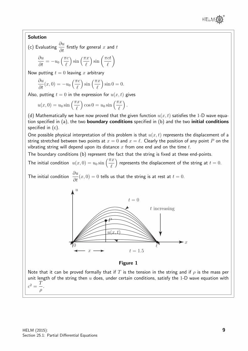
(d) Mathematically we have now proved that the given function u(x, t) satisfies the 1-D wave equa-tion specified in (a), the two boundary conditions specified in (b) and the two initial conditionsspecified in (c).

One possible physical interpretation of this problem is that u(x, t) represents the displacement of astring stretched between two points at x = 0 and x = `. Clearly the position of any point P on thevibrating string will depend upon its distance x from one end and on the time t.

The boundary conditions (b) represent the fact that the string is fixed at these end-points.

The initial condition u(x, 0) = u0 sin(πx`

)represents the displacement of the string at t = 0.

The initial condition∂u

∂t(x, 0) = 0 tells us that the string is at rest at t = 0.

t = 0

t = 1.5

t increasing

�0

u

x

P

u(x, t)

x

Figure 1

Note that it can be proved formally that if T is the tension in the string and if ρ is the mass perunit length of the string then u does, under certain conditions, satisfy the 1-D wave equation with

c2 =T

ρ.


9

Key Point 4

The three PDEs of greatest general interest involving two independent variables are:

(a) The two-dimensional Laplace equation

∂2u

∂x2+∂2u

∂y2= 0

(b) The one-dimensional heat conduction equation:

∂2u

∂x2=

1

k

∂u

∂tor

∂u

∂t= k

∂2u

∂x2

(c) The one-dimensional wave equation:

∂2u

∂x2=

1

c2∂2u

∂t2or

∂2u

∂t2= c2

∂2u

∂x2


®

Applications of PDEs��

��25.2

IntroductionIn this Section we discuss briefly some of the most important PDEs that arise in various branchesof science and engineering. We shall see that some equations can be used to describe a variety ofdifferent situations.

�

�

�

�Prerequisites


• have a knowledge of partial differentiation

�

�

�



• recognise the heat conduction equation andthe wave equation and have some knowledgeof their applicability

HELM (2015):Section 25.2: Applications of PDEs

11

Key Point 4 by no means exhausts the types of PDE which are important in applications. In thisSection we will discuss those three PDEs in Key Point 4 in more detail and briefly discuss other PDEsover a wide range of applications. We will omit detailed derivations.

1. Wave equationThe simplest situation to give rise to the one-dimensional wave equation is the motion of a stretchedstring - specifically the transverse vibrations of a string such as the string of a musical instrument.Assume that a string is placed along the x-axis, is stretched and then fixed at ends x = 0 and x = L;it is then deflected and at some instant, which we call t = 0, is released and allowed to vibrate. Thequantity of interest is the deflection u of the string at any point x, 0 ≤ x ≤ L, and at any timet > 0. We write u = u(x, t). Figure 2 shows a possible displacement of the string at a fixed time t.

u=u

x

u(x, t)

L0

Figure 2

Subject to various assumptions · · ·

1. damping forces such as air resistance are negligible

2. the weight of the string is negligible

3. the tension in the string is tangential to the curve of the string at any point

4. the string performs small transverse oscillations i.e. every particle of the string moves strictlyvertically and such that its deflection and slope as every point on the string is small.

· · · it can be shown, by applying Newton’s law of motion to a small segment of the string, that usatisfies the PDE

∂2u

∂t2= c2

∂2u

∂x2(1)

where c2 =T

ρ, ρ being the mass per unit length of the string and T being the (constant) horizontal

component of the tension in the string. To determine u(x, t) uniquely, we must also know

1. the initial definition of the string at the time t = 0 at which it is released

2. the initial velocity of the string.

Thus we must be given initial conditions

u (x, 0) = f(x) 0 ≤ x ≤ L (initial position)

∂u

∂t(x, 0) = g(x) 0 ≤ x ≤ L (initial velocity)

where f(x) and g(x) are known.


®

These two initial conditions are in addition to the two boundary conditions

u(0, t) = u(L, t) = 0 for t ≥ 0

which indicate that the string is fixed at each end. In Example 2 discussed in Section 25.1 we had

f(x) = u0 sin(πx`

)g(x) = 0 (string initially at rest).

The PDE (1) is the (undamped) wave equation. We will discuss solutions of it for various initialconditions later. More complicated forms of the wave equation would arise if some of the assumptionswere modified. For example:

(a)∂2u

∂t2= c2

∂2u

∂x2− g if the weight of the string was allowed for,

(b)∂2u

∂t2= c2

∂2u

∂x2− α

∂u

∂tif a damping force proportional to the velocity of the string

(with damping constant α) was included.

Equation (1) is referred to as the one-dimensional wave equation because only one space variable, x,is present. The two-dimensional (undamped) wave equation is, in Cartesian coordinates,

∂2u

∂t2= c2

(∂2u

∂x2+∂2u

∂y2

)(2)

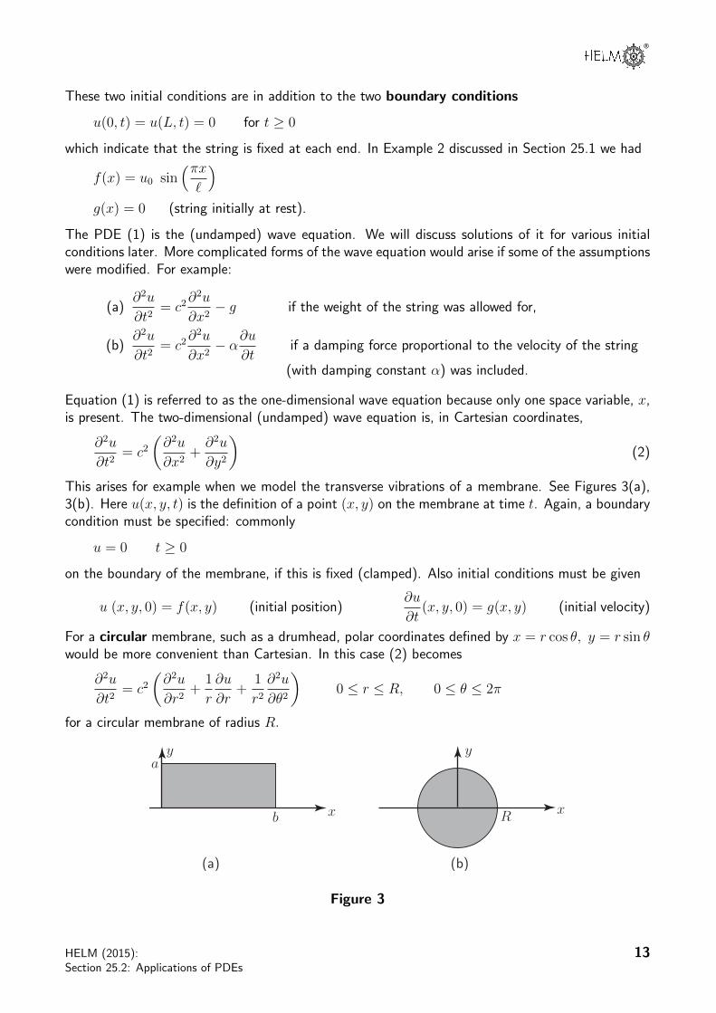
This arises for example when we model the transverse vibrations of a membrane. See Figures 3(a),3(b). Here u(x, y, t) is the definition of a point (x, y) on the membrane at time t. Again, a boundarycondition must be specified: commonly

u = 0 t ≥ 0

on the boundary of the membrane, if this is fixed (clamped). Also initial conditions must be given

u (x, y, 0) = f(x, y) (initial position)∂u

∂t(x, y, 0) = g(x, y) (initial velocity)

For a circular membrane, such as a drumhead, polar coordinates defined by x = r cos θ, y = r sin θwould be more convenient than Cartesian. In this case (2) becomes

∂2u

∂t2= c2

(∂2u

∂r2+

1

r

∂u

∂r+

1

r2∂2u

∂θ2

)0 ≤ r ≤ R, 0 ≤ θ ≤ 2π

for a circular membrane of radius R.

y

x

a

b

y

xR

(a) (b)

Figure 3


13

2. Heat conduction equationConsider a long thin bar, or wire, of constant cross-section and of homogeneous material orientedalong the x-axis (see Figure 4).

xx=Lx= 0

Figure 4

Imagine that the bar is thermally insulated laterally and is sufficiently thin that heat flows (byconduction) only in the x-direction. Then the temperature u at any point in the bar depends onlyon the x-coordinate of the point and the time t. By applying the principle of conservation of energyit can be shown that u(x, t) satisfies the PDE

∂u

∂t= k

∂2u

∂x20 ≤ x ≤ Lt ≥ 0

(3)

where k is a positive constant. In fact k, sometimes called the thermal diffusivity of the bar, isgiven by

k =κ

sρ

where κ = thermal conductivity of the material of the bar

s = specific heat capacity of the material of the bar

ρ = density of the material of the bar.

The PDE (3) is called the one-dimensional heat conduction equation (or, in other contexts where itarises, the diffusion equation).

TaskWhat is the obvious difference between the wave equation (1) and the heat con-duction equation (3)?

Your solution

AnswerBoth equations involve second derivatives in the space variable x but whereas the wave equation hasa second derivative in the time variable t the heat conduction equation has only a first derivative int. This means that the solutions of (3) are quite different in form from those of (1) and we shallstudy them separately later.


®

The fact that (3) is first order in t means that only one initial condition at t = 0 is needed, togetherwith two boundary conditions, to obtain a unique solution. The usual initial condition specifies theinitial temperature distribution in the bar

u(x, 0) = f(x)

where f(x) is known. Various types of boundary conditions at x = 0 and x = L are possible. Forexample:

(a) u(0, t) = T1 and u(L, t) = T2 (ends of the bar are at constant temperatures T1 and T2).

(b)∂u

∂x(0, t) =

∂u

∂x(L, t) = 0 which are insulation conditions since they tell us that there is

no heat flow through the ends of the bar.

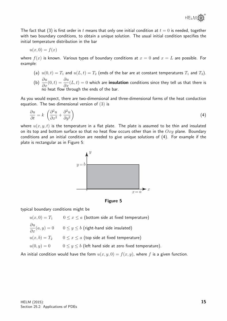
As you would expect, there are two-dimensional and three-dimensional forms of the heat conductionequation. The two dimensional version of (3) is

∂u

∂t= k

(∂2u

∂x2+∂2u

∂y2

)(4)

where u(x, y, t) is the temperature in a flat plate. The plate is assumed to be thin and insulatedon its top and bottom surface so that no heat flow occurs other than in the Oxy plane. Boundaryconditions and an initial condition are needed to give unique solutions of (4). For example if theplate is rectangular as in Figure 5:

xx= a

y= b

y

Figure 5

typical boundary conditions might be

u(x, 0) = T1 0 ≤ x ≤ a (bottom side at fixed temperature)

∂u

∂x(a, y) = 0 0 ≤ y ≤ b (right-hand side insulated)

u(x, b) = T2 0 ≤ x ≤ a (top side at fixed temperature)

u(0, y) = 0 0 ≤ y ≤ b (left hand side at zero fixed temperature).

An initial condition would have the form u(x, y, 0) = f(x, y), where f is a given function.


15

3. Transmission line equationsIn a long electrical cable or a telephone wire both the current and voltage depend upon positionalong the wire as well as the time (see Figure 6).

x

v(x, t)

i(x, t)

i(x, t)

Figure 6

It is possible to show, using basic laws of electrical circuit theory, that the electrical current i(x, t)satisfies the PDE

∂2i

∂x2= LC

∂2i

∂t2+ (RC +GL)

∂i

∂t+RGi (5)

where the constants R,L,C and G are, for unit length of cable, respectively the resistance, induc-tance, capacitance and leakage conductance. The voltage v(x, t) also satisfies (5). Special cases of(5) arise in particular situations. For a submarine cable G is negligible and frequencies are low soinductive effects can also be neglected. In this case (5) becomes

∂2i

∂x2= RC

∂i

∂t(6)

which is called the submarine equation or telegraph equation. For high frequency alternatingcurrents, again with negligible leakage, (5) can be approximated by

∂2i

∂x2= LC

∂2i

∂t2(7)

which is called the high frequency line equation.

TaskWhat PDEs, already discussed, have the same form as equations (6) or (7)?

Your solution

Answer(6) has the same form as the one-dimensional heat conduction equation.

(7) has the same form as the one-dimensional wave equation.


®

4. Laplace’s equationIf you look back at the two-dimensional heat conduction equation (4):

∂u

∂t= k

(∂2u

∂x2+∂2u

∂y2

)it is clear that if the heat flow is steady, i.e. time independent, then

∂u

∂t= 0 so the temperature

u(x, y) is a solution of

∂2u

∂x2+∂2u

∂y2= 0 (8)

(8) is the two-dimensional Laplace equation. Both this, and its three-dimensional counterpart

∂2u

∂x2+∂2u

∂y2+∂2u

∂z2= 0 (9)

arise in a wide variety of applications, quite apart from steady state heat conduction theory. Sincetime does not arise in (8) or (9) it is evident that Laplace’s equation is always a model for equilibriumsituations. In any problem involving Laplace’s equation we are interested in solving it in a specificregion R for given boundary conditions. Since conditions may involve

(a) u specified on the boundary curve C (two dimensions) or boundary surface S (threedimensions) of the region R. Such boundary conditions are called Dirichlet conditions.

(b) The derivative of u normal to the boundary, written∂u

∂n, specified on C or S. These are

referred to as Neumann boundary conditions.

(c) A mixture of (a) and (b).

Some areas in which Laplace’s equation arises are

(a) electrostatics (u being the electrostatic potential in a charge free region)

(b) gravitation (u being the gravitational potential in free space)

(c) steady state flow of inviscid fluids

(d) steady state heat conduction (as already discussed)


17

5. Other important PDEs in science and engineering

1. Poisson’s equation

∂2u

∂x2+∂2u

∂y2= f(x, y) (two-dimensional form)

where f(x, y) is a given function. This equation arises in electrostatics, elasticity theory andelsewhere.

2. Helmholtz’s equation

∂2u

∂x2+∂2u

∂y2+ k2u = 0 (two dimensional form)

which arises in wave theory.

3. Schrodinger’s equation

− h2

8π2m

(∂2ψ

∂x2+∂2ψ

∂y2+∂2ψ

∂z2

)= Eψ

which arises in quantum mechanics. (h is Planck’s constant)

4. Transverse vibrations equation

a2∂4u

∂x4+∂2u

∂t2= 0

for a homogeneous rod, where u(x, t) is the displacement at time t of the cross section throughx.

All the PDEs we have discussed are second order (because the highest order derivatives that ariseare second order) apart from the last example which is fourth order.


®

Solution UsingSeparation of Variables

��

��25.3

IntroductionThe main topic of this Section is the solution of PDEs using the method of separation of variables.In this method a PDE involving n independent variables is converted into n ordinary differentialequations. (In this introductory account n will always be 2.)

You should be aware that other analytical methods and also numerical methods are available forsolving PDEs. However, the separation of variables technique does give some useful solutions toimportant PDEs.

�

�

�

�Prerequisites


• be able to solve first and second orderconstant coefficient ordinary differentialequations'

&

$

%Learning Outcomes


• apply the separation of variables method toobtain solutions of the heat conductionequation, the wave equation and the 2-DLaplace equation for specified boundary orinitial conditions

HELM (2015):Section 25.3: Solution Using Separation of Variables

19

1. Solution of important PDEsWe shall just consider two analytic solution techniques for PDEs:

(a) Direct integration

(b) Separation of variables

The method of direct integration is a straightforward extension of solving very simple ODEs byintegration, and will be considered first. The method of separation of variables is more importantand we will study it in detail shortly.

You should note that many practical problems involving PDEs have to be solved by numericalmethods but that is another story (introduced in 32 and 33).

TaskSolve the ODE

d2y

dx2= x2 + 2

given that y = 1 when x = 0 anddy

dx= 2 when x = 0.

First finddy

dxby integrating once, not forgetting the arbitrary constant of integration:

Your solution

Answerdy

dx=x3

3+ 2x+ A

Now find y by integrating again, not forgetting to include another arbitrary constant:

Your solution

Answer

y =x4

12+ x2 + Ax+B

Now find A and B by inserting the two given initial conditions and so find the solution:

Your solution

Answery(0) = 1 gives B = 1 y′(0) = 2 gives A = 2

so the required solution is

y =x4

12+ x2 + 2x+ 1


®

Consider now a similar type of PDE i.e. one that can also be solved by direct integration.Suppose we require the general solution of

∂2u

∂x2= 2xet

where u is a function of x and t.Integrating with respect to x gives us

∂u

∂x= x2et + f(t)

where the arbitrary function f(t) replaces the normal “arbitrary constant” of ordinary integration.This function of t only is needed because we are integrating “partially” with respect to x i.e. we arereversing a partial differentiation with respect to x at constant t.Integrating again with respect to x gives the general solution:

u =x3

3et + x f(t) + g(t)

where g(t) is a second arbitrary function. We have now obtained the general solution of the givenPDE but to find the arbitrary function we must know two initial conditions.Suppose, for the sake of example, that these conditions are

u(0, t) = t ,∂u

∂x(0, t) = et

Inserting the first of these conditions into the general solution gives g(t) = t.

Inserting the second condition into the general solution gives f(t) = et.

So the final solution is u =x3

3et + xet + t.

TaskSolve the PDE

∂2u

∂x∂y= sinx cos y

subject to the conditions

∂u

∂x= 2x at y =

π

2, u = 2 sin y at x = π.

First integrate the PDE with respect to y: (it is equally valid to integrate first with respect to x).Don’t forget the appropriate arbitrary function.

Your solution


21

Answer

Recall that∂2u

∂x∂y=

∂

∂y

(∂u

∂x

)Hence integration with respect to y gives

∂u

∂x= sinx sin y + f(x)

Since one of the given conditions is on∂u

∂x, impose this condition to determine the arbitrary function

f(x):

Your solution

AnswerAt y = π/2 the condition gives sinx sin π/2 + f(x) = 2x i.e. f(x) = 2x− sinx

So∂u

∂x= sinx sin y + 2x− sinx

Now integrate again to determine u:

Your solution

AnswerIntegrating now with respect to x gives u = − cosx sin y + x2 + cosx+ g(y)

Next, obtain the arbitrary function g(y):

Your solution

AnswerThe condition u(π, y) = 2 sin y gives − cos π sin y + π2 + cos π + g(y) = 2 sin y

∴ sin y + π2 − 1 + g(y) = 2 sin y

∴ g(y) = sin y + 1− π2

Now write down the final answer for u(x, y):

Your solution

Answer

u(x, y) = x2 + cosx(1− sin y) + sin y + 1− π2


®

2. Method of separation of variables - general approachIn Section 25.2 we showed that

(a) u(x, y) = sin x cosh y

is a solution of the two-dimensional Laplace equation

(b) u(x, t) = e−2π2t sin πx

is a solution of the one-dimensional heat conduction equation

(c) u(x, t) = u0 sin(πx`

)cos

(πct

`

)is a solution of the one-dimensional wave equation.

All three solutions here have a specific form: in (a) u(x, y) is a product of a function of x alone,sinx, and a function of y alone, cosh y. Similarly, in both (b) and (c), u(x, t) is a product of afunction of x alone and a function of t alone.

The method of separation of variables involves finding solutions of PDEs which are of this productform. In the method we assume that a solution to a PDE has the form.

u(x, t) = X(x)T (t) (or u(x, y) = X(x)Y (y))

where X(x) is a function of x only, T (t) is a function of t only and Y (y) is a function y only.

You should note that not all solutions to PDEs are of this type; for example, it is easy to verify that

u(x, y) = x2 − y2

(which is not of the form u(x, y) = X(x)Y (y)) is a solution of the Laplace equation.

However, many interesting and useful solutions of PDEs are obtainable which are of the productform. We shall firstly consider the types of solution obtainable for our three basic PDEs using trialsolutions of the product form.

Heat conduction equation

∂2u

∂x2=

1

k

∂u

∂tk > 0 (1)

Assuming that

u = X(x)T (t)

= XT for short

(2)

then

∂u

∂x=

dX

dxT = X ′T for short

∂2u

∂x2=

d2X

dx2T = X ′′T for short

∂u

∂t= X

dT

dt= XT ′ for short


23

Substituting into the original PDE (1)

X ′′T =1

kXT ′

which can be re-arranged as

X ′′

X=

1

k

T ′

T(3)

Now the left-hand side of (3) involves functions of x only and the right-hand side expression containfunctions of t only. Thus altering the value of t cannot change the left-hand side of (3) i.e. it staysconstant. Hence so must the right-hand side be constant. We conclude that T (t) is a function suchthat

1

k

T ′

T= K (4)

where K is a constant whose sign is yet to be determined.

By a similar argument, altering the value of x cannot change the right-hand side of (3) and conse-quently the left-hand side must be a constant, i.e.

X ′′

X= K (5)

We see that the effect of assuming a product trial solution of the form (2) converts the PDE (1)into the two ODEs (4) and (5).

Both these ODEs are types whose solution we revised at the beginning of this Workbook but we shallnot attempt to solve them yet. In particular the solution of (5) depends on whether the constant Kis positive or negative.

Wave equation

∂2u

∂x2=

1

c2∂2u

∂t2(6)

TaskBy following a similar procedure to the above, assume a product solution

u(x, t) = X(x)T (t)

for the wave equation and find the two ODEs satisfied by X(x) and T (t).

First obtain∂2u

∂x2and

∂2u

∂t2:

Your solution

Answer

u = X(x)T (t) gives∂2u

∂x2= X ′′T and

∂2u

∂t2= XT ′′


®

Now substitute these results into (6) and transpose so the variables are separated i.e. all functionsof x are on the left-hand side, all funtions of t on the right-hand side:

Your solution

Answer

We get X ′′T =1

c2XT ′′ and, transposing,

X ′′

X=

1

c2T ′′

T

Finally, write down the required ordinary differential equations:

Your solution

AnswerEquating both sides to the same constant K gives

X ′′

X= K or

d2X

dx2−KX = 0 (7)

and

1

c2T ′′

T= K or

d2T

dt2−Kc2T = 0 (8)

The solution of the ODEs (7) and (8) has been obtained earlier, and will depend on the sign of K.

Laplace’s equation

∂2u

∂x2+∂2u

∂y2= 0 (9)

TaskSeparating the variables for Laplace’s equation follows similar lines to the previousTask. Obtain the ODEs satisfied by X(x) and Y (y).

Your solution


25

Answer

Assuming u(x, y) = X(x)Y (y) leads to:∂2u

∂x2= X ′′Y

∂2u

∂y2= XY ′′ so

X ′′Y +XY ′′ = 0 orX ′′

X= −Y

′′

Y

Equating each side to a constant K

X ′′

X= K or

d2X

dx2−KX = 0 (10a)

Y ′′

Y= −K or

d2Y

dy2+KY = 0 (10b)

(Note carefully the different signs in the two ODEs. Yet again the sign of the “separation constant”K will determine the solutions.)

3. Method of separation of variables - specific solutionsWe shall now study some specific problems which can be fully solved by the separation of variablesmethod.

Example 3Solve the heat conduction equation

∂2u

∂x2=

1

2

∂u

∂t

over 0 < x < 3, t > 0 for the boundary conditions

u(0, t) = u(3, t) = 0

and the initial condition

u(x, 0) = 5 sin 4πx.

Solution

Assuming u(x, t) = X(x)T (t) gives rise to the differential equations (4) and (5) with the parameterk = 2:

dT

dt= 2KT

d2X

dx2= KX


®

The T equation has general solution

T = Ae2Kt

which will increase exponentially with increasing t if K is positive and decrease with t if K is negative.In any physical problem the latter is the meaningful situation. To emphasise that K is being takenas negative we put

K = −λ2

so

T = Ae−2λ2t.

The X equation then becomes

d2X

dx2= −λ2X

which has solution

X(x) = B cosλx+ C sinλx.

Hence

u(x, t) = X(x)T (t) = (D cosλx+ E sinλx)e−2λ2t (11)

where D = AB and E = AC.

(You should always try to keep the number of arbitrary constants down to an absolute minimum bymultiplying them together in this way.)

We now insert the initial and boundary conditions to obtain the constant D andE and also theseparation constant λ.The initial condition u(0, t) = 0 gives

(D cos 0 + E sin 0)e−2λ2t = 0 for all t.

Since sin 0 = 0 and cos 0 = 1 this must imply that D = 0.The other initial condition u(3, t) = 0 then gives

E sin(3λ)e−2λ2t = 0 for all t.

We cannot deduce that the constant E has to be zero because then the solution (11) would be thetrivial solution u ≡ 0. The only sensible deduction is that

sin 3λ = 0 i.e. 3λ = nπ (where n is some integer).Hence solutions of the form (11) satisfying the 2 boundary conditions have the form

u(x, t) = En sin(nπx

3

)e−

2n2π2t9

where we have written En for E to allow for the possibility of a different value for the constant foreach different value of n.

We obtain the value of n by using the initial condition u(x, 0) = 5 sin 4πx and forcing this solutionto agree with it. That is,

u(x, 0) = En sin(nπx

3

)= 5 sin 4πx


27

so we must choose n = 12 with E12 = 5.Hence, finally,

u(x, t) = 5 sin

(12πx

3

)e−

29(12)2π2t = 5 sin(4πx) e−32π

2t.

TaskSolve the 1-dimensional wave equation

∂2u

∂x2=

1

16

∂2u

∂t2for 0 < x < 2, t > 0

The boundary conditions are

u(0, t) = u(2, t) = 0

The initial conditions are

(i) u(x, 0) = 6 sin πx− 3 sin 4πx (ii)∂u

∂t(x, 0) = 0

Firstly, either using (7) and (8) or by working from first principles assuming the product solution

u(x, t) = X(x)T (t),

write down the ODEs satisfied by X(x) and T (t):

Your solution

AnswerX ′′

X= K

T ′′

16T= K

Now decide on the appropriate sign for K and then write down the solution to these equations:

Your solution

AnswerChoosing K as negative (say K = −λ2) will produce Sinusoidal solutions for X and T which areappropriate in the context of the wave equation where oscillatory solutions can be expected.

Then X ′′ = −λ2X gives

X = A cosλx+B sinλx

Similarly T ′′ = −16λ2T gives

T = C cos 4λt+D sin 4λt


®

Now obtain the general solution u(x, t) by multiplying X(x) by T (t) and insert the two boundaryconditions to obtain information about two of the constants:

Your solution

Answeru(x, t) = (A cosλx+B sinλx)(C cos 4λt+D sin 4λt)

u(0, t) = 0 for all t gives

A(C cos 4λt+D sin 4λt) = 0

which implies that A = 0.

u(2, t) = 0 for all t gives

B sin 2λ(C cos 4λt+D sin 4λt) = 0

so, for a non-trivial solution,

sin 2λ = 0 i.e. λ =nπ

2for some integer n.

At this stage we write the solution as

u(x, t) = sin(nπx

2

)(E cos 2nπt+ F sin 2nπt)

where we have multiplied constants and put E = BC and F = BD.


29

Now insert the initial condition

∂u

∂t(x, 0) = 0 for all x 0 < x < 2.

and deduce the value of F :

Your solution

AnswerDifferentiating partially with respect to t

∂u

∂t= sin

(nπx2

)(−2nπE sin 2nπt+ 2nπF cos 2nπt)

so at t = 0

∂u

∂t(x, 0) = sin

(nπx2

)2nπF = 0

from which we must have that F = 0.

Finally using the other the initial condition u(x, 0) = 6 sin(πx) − 3 sin(4πx) deduce the form ofu(x, t):

Your solution


®

AnswerAt this stage the solution reads

u(x, t) = E sin(nπx

2

)cos(2nπt) (12)

We now have to insert the last condition i.e. the initial condition

u(x, 0) = 6 sin πx− 3 sin 4πx (13)

This seems strange because, putting t = 0 in our solution (12) suggests

u(x, 0) = E sin(nπx

2

)At this point we seem to have incompatability because no single value of n will enable us to satisfy(13). However, in the solution (12), any positive integer value of n is acceptable and we can infact, superpose solutions of the form (12) and still have a valid solution to the PDE Hence we firstwrite, instead of (12)

u(x, t) =∞∑n=1

En sin(nπx

2

)cos(2nπt) (14)

from which

u(x, 0) =∞∑n=1

En sin(nπx

2

)(15)

(which looks very much like, and indeed is, a Fourier series.)

To make the solution (15) fit the initial condition (13) we do not require all the terms in the infiniteFourier series. We need only the terms with n = 2 with coefficient E2 = 6 and the term for whichn = 8 with E8 = −3. All the other coefficients En have to be chosen as zero.

Using these results in (14) we obtain the solution

u(x, t) = 6 sin πx cos 4πt− 3 sin 4πx cos 16πt

The above solution perhaps seems rather involved but there is a definite sequence of logical stepswhich can be readily applied to other similar problems.


31

Engineering Example 1

Heat conduction through a furnace wall

Introduction

Conduction is a mode of heat transfer through molecular collision inside a material without anymotion of the material as a whole. If one end of a solid material is at a higher temperature, thenheat will be transferred towards the colder end because of the relative movement of the particles.They will collide with the each other with a net transfer of energy.

Energy flows through heat conductive materials by a thermal process generally known as ’gradientheat transport’. Gradient heat transport depends on three quantities: the heat conductivity of thematerial, the cross-sectional area of the material which is available for heat transfer and the spatialgradient of temperature (driving force for the process). The larger the conductivity, the gradient,and the cross section, the faster the heat flows.

The temperature profile within a body depends upon the rate of heat transfer to the atmosphere,its capacity to store some of this heat, and its rate of thermal conduction to its boundaries (wherethe heat is transferred to the surrounding environment). Mathematically this is stated by the heatequation

∂

∂x

(k∂T

∂x

)= ρc

∂T

∂x(1)

The thermal diffusivity α is related to the thermal conductivity k, the specific heat c, and the densityof solid material ρ, by

α =k

ρc

Problem in Words

The wall (thickness L) of a furnace, with inside temperature 800◦ C, is comprised of brick material[thermal conductivity = 0.02 W m−1 K−1)]. Given that the wall thickness is 12 cm, the atmospherictemperature is 0◦ C, the density and heat capacity of the brick material are 1.9 gm cm−3 and6.0 J kg−1 K−1 respectively, estimate the temperature profile within the brick wall after 2 hours.

Mathematical statement of problemSolve the partial differential equation

∂

∂x

(k∂T

∂x

)= ρc

∂T

∂t(2)

subject to the initial condition

T (x, 0) = 800 sinπx

2L(3)


®

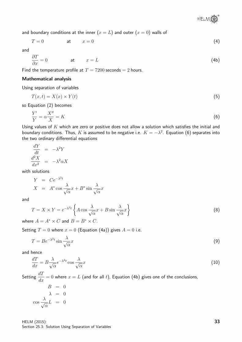
and boundary conditions at the inner (x = L) and outer (x = 0) walls of

T = 0 at x = 0 (4)

and

∂T

∂x= 0 at x = L (4b)

Find the temperature profile at T = 7200 seconds = 2 hours.

Mathematical analysis

Using separation of variables

T (x, t) = X(x)× Y (t) (5)

so Equation (2) becomes

Y ′

Y= α

X ′′

X= K (6)

Using values of K which are zero or positive does not allow a solution which satisfies the initial andboundary conditions. Thus, K is assumed to be negative i.e. K = −λ2. Equation (6) separates intothe two ordinary differential equations

dY

dt= −λ2Y

d2X

dx2= −λ2αX

with solutions

Y = Ce−λ2t

X = A∗ cosλ√αx+B∗ sin

λ√αx

and

T = X × Y = e−λ2t

{A cos

λ√αx+B sin

λ√αx

}(8)

where A = A∗ × C and B = B∗ × C.

Setting T = 0 where x = 0 (Equation (4a)) gives A = 0 i.e.

T = Be−λ2t sin

λ√αx (9)

and hence

dT

dx= B

λ√αe−λ

2t cosλ√αx (10)

SettingdT

dx= 0 where x = L (and for all t), Equation (4b) gives one of the conclusions,

B = 0

λ = 0

cosλ√αL = 0


33

The first two possibilities (B = 0 and λ = 0) can be discounted as they leave T = 0 for all x and t

and it is not possible to satisfy the initial condition (3). Hence cosλ√αL = 0 so

λ√αL = (n + 1

2)π

and we deduce that

λ =

√α

L(n+

1

2)π (11)

and so the temperature T satisfies

T = Be−α

L2(n+ 1

2)2t

sin

{(n+

1

2)πx

L

}(12)

However, this must also satisfy Equation (2) i.e.

800 sinπx

2L= B sin

{(n+

1

2)πx

L

}(13)

Equating the arguments of the sine terms

πx

2L= (n+

1

2)πx

Lso n = 0

Equating the coefficients of the sine terms

800 = B

So the temperature profile is

T = 800e−αt2L2 sin

πx

2L(14)

where α =k

ρc=

0.02

1900× 6= 1.764× 10−6m2s−1.

After two hours, t = 7200 so − αt

2L2= −0.438 so

T = 800× e−0.438 sin πx2L

= 516 sinπx

2L(15)

so the inner wall of the furnace has cooled from 800◦C to 516◦C.

Interpretation

The boundary conditions (2) and (3) represent approximations to the true boundary conditions,approximations made to enable solution by separation of variables. More realistic conditions wouldbe

−k∂T (0, t)∂x

= houtside {T∞ − T (0, t)}

−k∂T (L, t)∂x

= hinside {T (0, t)− Ts}


®

Solution UsingFourier Series

��

��25.4

IntroductionIn this Section we continue to use the separation of variables method for solving PDEs but you willfind that, to be able to fit certain boundary conditions, Fourier series methods have to be used leadingto the final solution being in the (rather complicated) form of an infinite series. The techniques will beillustrated using the two-dimensional Laplace equation but similar situations often arise in connectionwith other important PDEs.

�

�

�

�Prerequisites


• be familiar with the separation of variablesmethod

• be familiar with trigonometric Fourier series�

�

�



• solve the 2-D Laplace equation for givenboundary conditions and utilize Fourier seriesin the solution when necessary

HELM (2015):Section 25.4: Solution Using Fourier Series

35

1. Solutions involving infinite Fourier seriesWe shall illustrate this situation using Laplace’s equation but infinite Fourier series can also benecessary for the heat conduction and wave equations.

We recall from the previous Section that using a product solution

u(x, t) = X(x)Y (y)

in Laplace’s equation gives rise to the ODEs:

X ′′

X= K

Y ′′

Y= −K

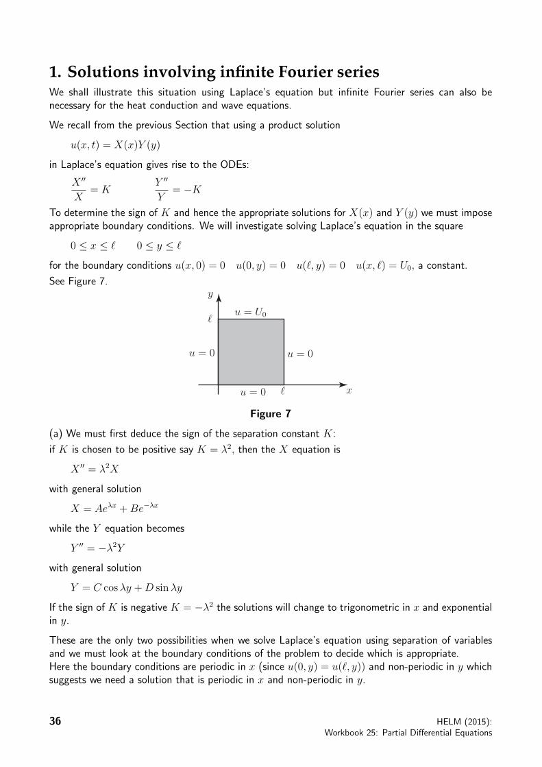
To determine the sign of K and hence the appropriate solutions for X(x) and Y (y) we must imposeappropriate boundary conditions. We will investigate solving Laplace’s equation in the square

0 ≤ x ≤ ` 0 ≤ y ≤ `

for the boundary conditions u(x, 0) = 0 u(0, y) = 0 u(`, y) = 0 u(x, `) = U0, a constant.

See Figure 7.

x�

u = U0

u = 0

y

u = 0

u = 0

�

Figure 7

(a) We must first deduce the sign of the separation constant K:

if K is chosen to be positive say K = λ2, then the X equation is

X ′′ = λ2X

with general solution

X = Aeλx +Be−λx

while the Y equation becomes

Y ′′ = −λ2Ywith general solution

Y = C cosλy +D sinλy

If the sign of K is negative K = −λ2 the solutions will change to trigonometric in x and exponentialin y.

These are the only two possibilities when we solve Laplace’s equation using separation of variablesand we must look at the boundary conditions of the problem to decide which is appropriate.Here the boundary conditions are periodic in x (since u(0, y) = u(`, y)) and non-periodic in y whichsuggests we need a solution that is periodic in x and non-periodic in y.


®

Thus we choose K = −λ2 to give

X(x) = (A cosλx+B sinλx)

Y (y) = (Ceλy +De−λy)

(Note that had we chosen the incorrect sign for K at this stage we would later have found it impossibleto satisfy all the given boundary conditions. You might like to verify this statement.)

The appropriate general solution of Laplace’s equation for the given problem is

u(x, y) = (A cosλx+B sinλx)(Ceλy +De−λy).

(b) Inserting the boundary conditions produces the following consequences:

u(0, y) = 0 gives A = 0

u(`, y) = 0 gives sinλ` = 0 i.e. λ =nπ

`

where n is a positive integer 1, 2, 3, . . . . While n = 0 also satisfies the equation it leads to the trivialsolution u = 0 only.)

u(x, 0) = 0 gives C +D = 0 i.e. D = −CAt this point the solution can be written

u(x, y) = BC sin(nπx

`

)(e

nπy

` − e−nπy

`

)This can be conveniently written as

u(x, y) = E sin(nπx

`

)sinh

(nπy`

)(1)

where E = 2BC.

At this stage we have just one final boundary condition to insert to obtain information about theconstant E and the integer n. Our solution (1) gives

u(x, `) = E sin(nπx

`

)sinh(nπ)

and clearly this is not compatible, as it stands, with the given boundary condition

u(x, `) = U0 = constant.

The way to proceed is again to superpose solutions of the form (1) for all positive integer values ofn to give

u(x, y) =∞∑n=1

En sin(nπx

`

)sinh

(nπy`

)(2)

from which the final boundary condition gives

U0 =∞∑n=1

En sin(nπx

`

)sinh(nπ) 0 < x < `. (3)

=∞∑n=1

bn sin(nπx

`

)where bn = En sinh(nπ).


37

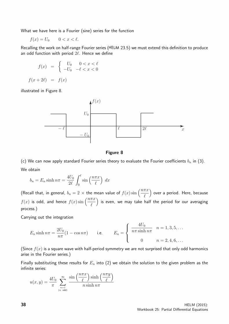
What we have here is a Fourier (sine) series for the function

f(x) = U0 0 < x < `.

Recalling the work on half-range Fourier series ( 23.5) we must extend this definition to producean odd function with period 2`. Hence we define

f(x) =

{U0 0 < x < `−U0 −` < x < 0

f(x+ 2`) = f(x)

illustrated in Figure 8.

x�

U0

− U0

2�− �

f(x)

Figure 8

(c) We can now apply standard Fourier series theory to evaluate the Fourier coefficients bn in (3).

We obtain

bn = En sinhnπ =4U0

2`

∫ `

0

sin(nπx

`

)dx

(Recall that, in general, bn = 2 × the mean value of f(x) sin(nπx

`

)over a period. Here, because

f(x) is odd, and hence f(x) sin(nπx

`

)is even, we may take half the period for our averaging

process.)

Carrying out the integration

En sinhnπ =2U0

nπ(1− cosnπ) i.e. En =

4U0

nπ sinhnπn = 1, 3, 5, . . .

0 n = 2, 4, 6, . . .

(Since f(x) is a square wave with half-period symmetry we are not surprised that only odd harmonicsarise in the Fourier series.)

Finally substituting these results for En into (2) we obtain the solution to the given problem as theinfinite series:

u(x, y) =4U0

π

∞∑n=1

(n odd)

sin(nπx

`

)sinh

(nπy`

)n sinhnπ


®

TaskSolve Laplace’s equation to determine the steady state temperature u(x, y) in thesemi-infinite plate 0 ≤ x ≤ 1, y ≥ 0. Assume that the left and right sides areinsulated and assume that the solution is bounded. The temperature along thebottom side is a known function f(x).

First write this problem as a mathematical boundary value problem paying particular attention to themathematical representation of the boundary conditions:

Your solution

AnswerSince the sides x = 0 and x = 1 are insulated, the temperature gradient across these sides is zero

i.e.∂u

∂x= 0 for x = 0, 0 < y <∞ and

∂u

∂x= 0 for x = 1, 0 < y <∞.

The third boundary condition is u(x, 0) = f(x).

The fourth boundary condition is less obvious: since the solution should be bounded (ie not growand grow) we must demand that u(x, y)→ 0 as y →∞. (See figure below.)

x

∂u

∂x= 0

u = f(x)0 1

y

∂u

∂x= 0


39

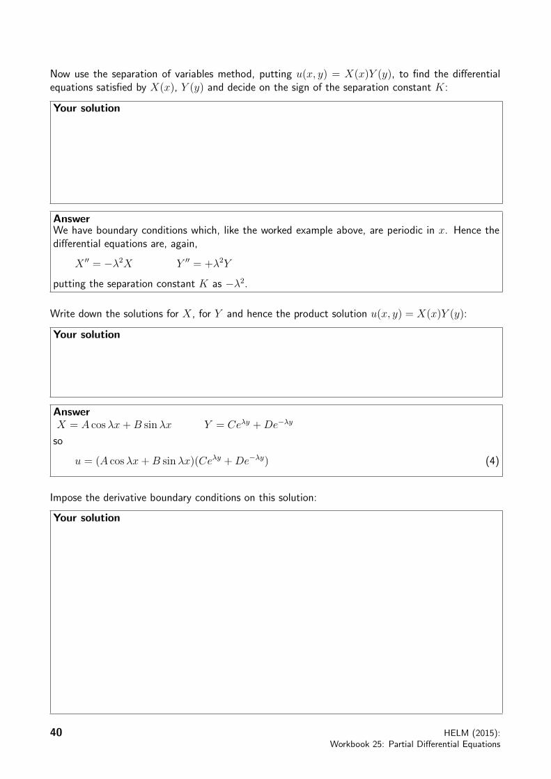
Now use the separation of variables method, putting u(x, y) = X(x)Y (y), to find the differentialequations satisfied by X(x), Y (y) and decide on the sign of the separation constant K:

Your solution

AnswerWe have boundary conditions which, like the worked example above, are periodic in x. Hence thedifferential equations are, again,

X ′′ = −λ2X Y ′′ = +λ2Y

putting the separation constant K as −λ2.

Write down the solutions for X, for Y and hence the product solution u(x, y) = X(x)Y (y):

Your solution

AnswerX = A cosλx+B sinλx Y = Ceλy +De−λy

so

u = (A cosλx+B sinλx)(Ceλy +De−λy) (4)

Impose the derivative boundary conditions on this solution:

Your solution


®

Answer

∂u

∂x= (−λA sinλx+ λB cosλx)(Ceλy +De−λy)

Hence∂u

∂x(0, y) = 0 gives λB(Ceλy +De−λy) = 0 for all y.

The possibility λ = 0 can be excluded this would give a trivial constant solution in (4). Hence wemust choose B = 0.

The condition∂u

∂x(1, y) = 0 gives

−λA sinλ(Ceλy +De−λy) = 0

Choosing A = 0 would make u ≡ 0 so we must force sinλ to be zero i.e. choose λ = nπ where nis a positive integer.

Thus, at this stage (4) becomes

u = A cosnπx(Cenπy +De−nπy)

= cosnπx(Eenπy + Fe−nπy) (5)

Now impose the condition that this solution should be bounded:

Your solution

AnswerThe region over which we are solving Laplace’s equation is semi-infinite i.e. the y coordinateincreases without limit. The solution for u(x, y) in (5) will increase without limit as y →∞ due tothe term enπy (n being a positive integer.) This can be avoided i.e. the solution will be bounded ifthe constant E is chosen as zero.

Finally, use Fourier series techniques to deal with the final boundary condition u(x, 0) = f(x):

Your solution


41

Your solution

AnswerSuperposing solutions of the form (5) (with E = 0) gives

u(x, y) =∞∑n=0

Fn cos(nπx) e−nπy (6)

so the boundary condition gives

f(x) =∞∑n=0

Fn cosnπx

We have here a half-range Fourier cosine series representation of a function f(x) defined over0 < x < 1. Extending f(x) as an even periodic function with period 2 and using standard Fourierseries theory gives

Fn = 2

∫ 1

0

f(x) cosnπx dx n = 1, 2, . . .

with

F0

2=

∫ 1

0

f(x) dx.

Hence (6) is the solution of this given boundary value problem, the integrals giving us in principlethe Fourier coefficients Fn for a given function f(x).


Index for Workbook 25

Auxiliary equation 4

Boundary conditions 8, 13, 15

Diffusion equation - see Heat conductionequation

Dirichlet conditions 17

Fourier series 35-42

Heat conduction 32Heat conduction equation 8, 14

23, 26, 32Helmholtz’s equation 18High frequency line equation 16

Initial conditions 3, 8, 12, 15Insulation conditions 15

Laplace’s equation 7, 17, 25, 36

Neumann boundary conditions 17

ODE - first order 3- second order 4, 6

Partial derivatives 6Poisson’s equation 18

Schrodinger’s equation 18Separation of variables 19-34Simple harmonic motion 6Submarine equation 16

Telegraph equation 16Transmission line equation 16Transverse vibrations equation 18

Wave equation 8, 12, 24, 28

ENGINEERING EXAMPLES1 Heat conduction through a furnace

wall 32

Di�erential equations 3-6

Documents

About+the+HELM+Project+nucinkis-lab.cc.ic.ac.uk/HELM/HELM_Workbooks_21-25/WB25-all.pdf · HELM (2015): Section 25.1: Partial Di erential Equations 7. The PDE in the above Task has