Embed Size (px)
Citation preview
Islamic University – Gaza
Deanship of Graduate Studies
Faculty of Information Technology
Abnormal Network Traffic Detection based
on Clustering and Classification Techniques:
DoS Case Study
A Thesis Submitted in Partial Fulfillment of the Requirement
for the Degree of Master in Information Technology
Prepared By
Hani Mohammed Rihan
120092718
Supervised By
Dr. Tawfiq S. Barhoom
2013/1434H

i
Acknowledgements
Praise is to Allah,
First and foremost, I wish to thank Allah for giving me
strength and courage to complete this thesis and research. I would
like to express my gratitude to my supervisor Dr. Tawfiq Barhoom,
for providing me the opportunity to develop this work over the
master years. He was not only a good advisor; he also introduced
me to several other people whom I’ve had the pleasure to work
with and learn from, thank them a lot.
Thanks to my parents who have given credit after God in all
things. Thanks a lot to my wife who has supported me
throughout my study.
Thanks a lot to my friend Dr. Said Alzebda who has reviewed my thesis. Thanks to my friends who encouraged me to make every effort and determination, Last but not least, I would like to thank my family members. Thank you for giving me the support and love to complete my work.
Hani M. Rihan

ii
Table of Contents
Acknowledgements ……………………………………………………….…………….. i
Table of Contents ……………………………………………………………………….. ii
List of Figures ………………………………………………………………………….. iv
List of Tables …………………………………………………………………………. v
List of Abbreviation ……………………………………………………………………. vii
Abstract …………………………………………………………………………………. ix
Chapter 1: Introduction ……………………………………………………………… 1
1.1 Intrusion Detection System ……………………………………………………. 1
1.2 Research Motivation ……………………………………………………………. 2
1.3 Statement of the problem ……………………………………………………….. 2
1.4 Research Objectives ……………………………………………………………. 2
1.4.1 Main Objectives …………………………………………………………… 2
1.4.2 Specific Objectives ………………………………………………………. 3
1.5 Research Scope and Limitation ………………………………………………... 3
1.6 Significant of the research …………………………………………………… 4
1.7 Research Methodology ………………………………………………………….. 4
1.8 Outline of the Thesis …………………………………………………………… 6
1.9 Summary ………… …………………………………………………………… 7
Chapter 2: Literature Review …………………………………………………………. 8
2.1 Anomalies Definition ……………………………………………………………. 8
2.1.1 Types of Anomalies ……………………………………………………… 8
2.1.2 Anomalous Classification ……………………………………………… 8
2.1.3 Denial of Service …………………………………………………………. 10
2.2 Intrusion Detection System Types …………………………………………… 11
2. 3 Intrusion Detection System Approaches ……………………………………….. 11
2.4 Machine Learning ……………………………………………………………….. 12
2.4.1 Supervised Learning ………………………………………………………. 12
2.4.2 Unsupervised Learning ……………………………………………………. 12
2.5 Data Mining ……………………………………………………………………... 13
2.5.1 Data Mining Tasks ………………………………………………………… 15
2.6 Clustering ………………………………………………………………………... 15
2.6.1 Clustering Classification Methods ………………………………………… 15
2.6.2 Clustering application …………………………………………………….. 17
2.6.3 Clustering Problems ………………………………………………………. 17

iii
2.6.4 Clustering quality indexes ………………………………………………… 19
2.9 K-Nearest Neighbors………………………………………………………….. 21
2.10 Abnormal Network Traffic Detection Goals ……………………………….. 21
2.11 Summary ………… …………………………………………………………… 22
Chapter 3: Related Work ……………………………………………………………. 23
3.1 Abnormal detection based on cluster size ……………………………………… 23
3.2 Abnormal detection based on distance metrics and outlier ……………………… 25
3.3 Abnormal detection based on fuzzy clustering ………………………………… 28
3.4 Abnormal detection based on classification techniques ………………………… 30
3.5 Summary ………… …………………………………………………………… 33
Chapter 4: Research Proposal and Methodology …………………………………… 35
4.1 Methodology Steps ……………………………………………………………… 35
4.2 Data Sets of Model ……………………………………………………………… 35
4.2.1 Data Collection ………………………………………………………. 35
4.2.2 Data Description ……………………………………………………… 37
4.2.3 Data Samples …………………………………………………………. 39
4.2.4 Data sets Attacks Types …………………………………………………… 39
4.3 Data Preprocessing and Feature Selection………………………………………. 40
4.3.1 Preprocessing data sets …………………………………………………. 43
4.3.2 Feature Selection ……………………………………………………… 41
4.3 Design and Build the Model ……………………………………………………. 42
4.3.1 The Base Line Experiment ………………………………………………… 42
4.3.2 Apply the model …………………………………………………………... 43
4.3.3 Label Clusters Strategy ……………………………………………………. 44
4.3.4 New Instances Labeling Strategy ………………………………………. 45
4.4 Evaluate the Model ……………………………………………………………… 45
4.5 The Proposed Model ……………………………………………………………. 48
4.6 Summary………… ……………………………………………………………. 51
Chapter 5: Experimental Result and Evaluation …………………………………… 53
Chapter 6: Conclusion and Future work …………………………………………… 73
References …………………………………………………………..………………… 76
Appendix A …………………………………………………………………..………. 81
iv
List of Figures
Figure (2.1): Data mining as a step in the process of knowledge discovery
14
Figure (2.2): K-Means output for different iterations
19
Figure (4.1): Simulation Network for the DARPA 1998 dataset
36
Figure (4.2): Experimental setup of DARPA 1998 dataset
36
Figure (4.3): The Proposed Model
52
Figure (5.1): Clustering Result using K-Means in Case 1
56
Figure (5.2): Labeled clusters’ instances result after first step
56
Figure (5.3): Labeled clusters result after second step
57
Figure (5.4): Clustering Result using K-Means in Case 2
60
Figure (5.5): Clusters’ Instances result after labeled in Case 2 (First Step)
60
Figure (5.6): Clusters result after labeled in Case 2 (Second Step)
61
Figure (5.7): Clustering Result before labeled in Case2
63
Figure (5.8): Clustering Label Result based real behavior class in Case2
64
Figure (5.9): Clustering label based real behavior class and threshold size
65
Figure (5.10): Clustering label only based real behavior class
65
Figure (5.11): Example on labeling new instance - First Method
67
Figure (5.12): Example on labeling new instance using labeled clusters - case2
68
Figure (5.13): Label instances using distance and centroid of clusters Case 1
69
Figure (5.14): Label instances using distance and centriod of clusters Case 2
70
Figure (5.15): Clusters Labeling Evaluation Measurements for Cases 2, 3
71
Figure (5.16): Instances Labeling Evaluation Measurements 72

v
List of Tables
Table (2.1): Anomaly class and its description
9
Table (3.1): Related Works Summary
34
Table (4.1): Basic features of individual TCP connections
37
Table (4.2): Content features within a connection suggested by domain knowledge
38
Table (4.3): Traffic features computed using a two-second time window
38
Table (4.4): Host-based Traffic Features
38
Table (4.5): Sample of data sets
39
Table (4.6): KDD Cup 99 Datasets type and counts
39
Table (4.7): KDD Cup 99 10% Datasets type and counts
39
Table (4.8): Protocol Types
40
Table (4.9): Service Types
40
Table (4.10): Flag Types
41
Table (4.11): Selected features of KDDCUP dataset
42
Table (4.12): Clustering Validation Computations
43
Table (4.13): Experiment Result of clustering techniques
43
Table (4.14): K-Means Parameter
44
Table (4.15): Confusion Matrix Structure
46
Table (4.16): Confusion Matrix Example
47
Table (4.17): The Proposed model Processes
51
Table (5.1): Training and Testing Dataset in Case 1
54
Table (5.2): Features Translation Codes in Case 1
55
vi
Table (5.3): K-Means Parameters in Case 1
55
Table (5.4): Clustering Result using K-Means in Case 1
55
Table (5.5): Labeled clusters’ instances result after first step
56
Table (5.6): Labeled clusters result after second step
57
Table (5.7): Confusion Matrix for labeling clusters
58
Table (5.8): Training and Testing Dataset in Case 2
58
Table (5.9): Features Translation Codes in Case 2
59
Table (5.10): K-Means Parameters in Case 2
59
Table (5.11): Clustering Result using K-Means in Case 2
59
Table (5.12): Clusters’ Instances result after labeled in Case 2 (First Step)
60
Table (5.13): Clusters result after labeled in Case 2 (Second Step)
61
Table (5.14): Confusion Matrices for clusters labeling in Case 2
62
Table (5.15): Labeled clusters result after second step (5% threshold)
62
Table (5.16): Clustering Result before labeled in Case2
62
Table (5.17): Clustering Label Result based real behavior class in Case2
63
Table (5.18): Confusion Matrix Result based real behavior class in Case2
63
Table (5.19): Euclidean Distance calculation time for labeling new instance
66
Table (5.20): Label instances using distance and centroid of clusters Case 1
68
Table (5.21): Confusion Matrix for labeling instances using distance and centroid of clusters
Case 1
69
Table (5.22): Label instances using distance for labeling instances using distance and centroid of
clusters Case 2
69
Table (5.23): Confusion Matrix for labeling instances using distance and centroid of clusters
Case 2
70
Table (5.24): Clusters Labeling Evaluation Measurements
71
Table (5.25): Instances Labeling Evaluation Measurements
72
Table (6.1): Abnormal Traffic Detection Comparison
74

vii
LIST OF ABBREVIATION
Denial of Service DoS
Intrusion Detection System IDS
True Positive TP
False Positive FP
True Negative TN
False Negative FN
Detection Rate DR
False Alarm Rate FAR
Knowledge Discovery and Data Mining KDD
Defense Advanced Research Projects Agency DAPRA
Massachusetts Institute of Technology MIT
Local Area Network LAN
Transmission Control Protocol TCP
Internet Control Message Protocol ICMP
User Datagram Protocol UDP
Address Resolution Protocol
ARP
Internet Protocol IP
Intrusion Detection and Prevention Systems IDPS
Network Intrusion Detection System NIDS
Host-based Intrusion Detection System HIDS
Davies Bouldin DB

viii
LIST OF ABBREVIATION
FCM
Fuzzy C Means
UCI University of California, Irvine
R2L User to Root Attacks
U2R Remote to User Attacks
Probe Probing
KNN K-Nearest-Neighbor
ix
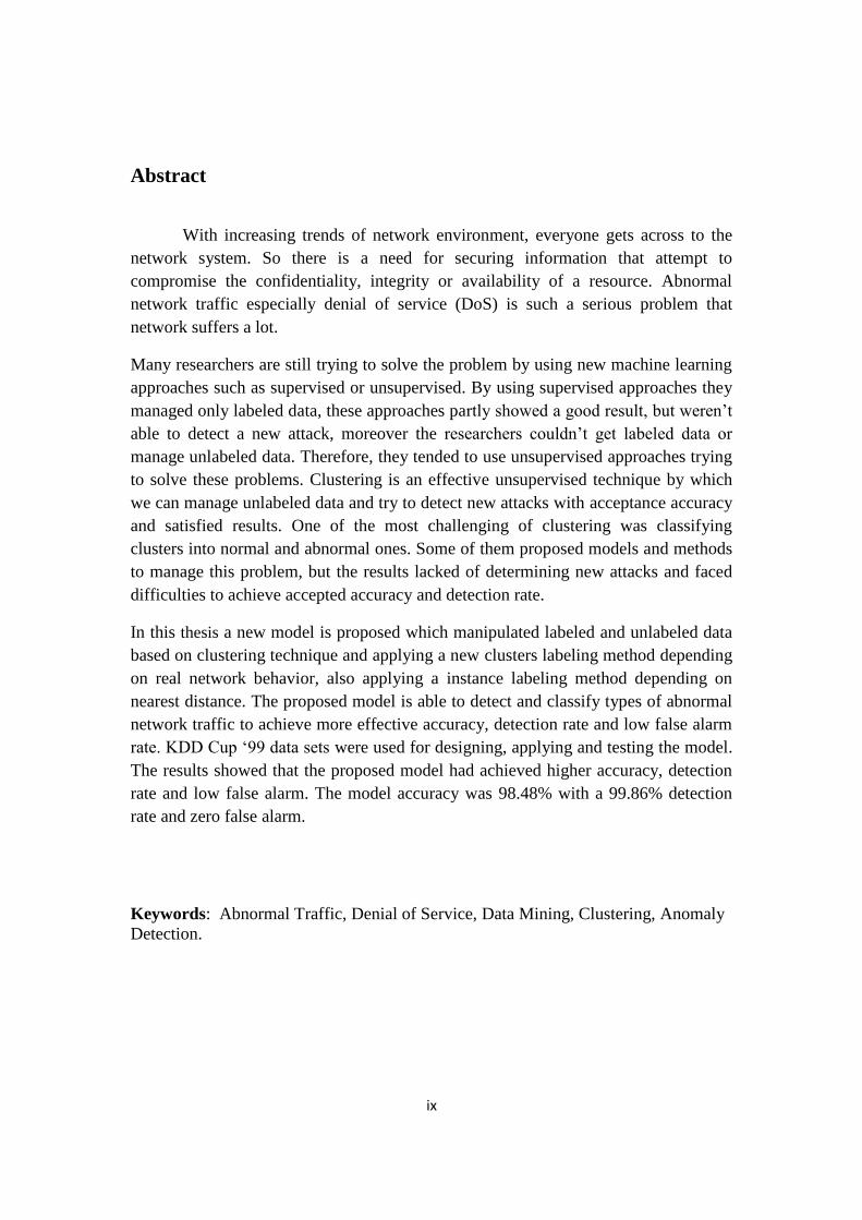
Abstract
With increasing trends of network environment, everyone gets across to the
network system. So there is a need for securing information that attempt to
compromise the confidentiality, integrity or availability of a resource. Abnormal
network traffic especially denial of service (DoS) is such a serious problem that
network suffers a lot.
Many researchers are still trying to solve the problem by using new machine learning
approaches such as supervised or unsupervised. By using supervised approaches they
managed only labeled data, these approaches partly showed a good result, but weren’t
able to detect a new attack, moreover the researchers couldn’t get labeled data or
manage unlabeled data. Therefore, they tended to use unsupervised approaches trying
to solve these problems. Clustering is an effective unsupervised technique by which
we can manage unlabeled data and try to detect new attacks with acceptance accuracy
and satisfied results. One of the most challenging of clustering was classifying
clusters into normal and abnormal ones. Some of them proposed models and methods
to manage this problem, but the results lacked of determining new attacks and faced
difficulties to achieve accepted accuracy and detection rate.
In this thesis a new model is proposed which manipulated labeled and unlabeled data
based on clustering technique and applying a new clusters labeling method depending
on real network behavior, also applying a instance labeling method depending on
nearest distance. The proposed model is able to detect and classify types of abnormal
network traffic to achieve more effective accuracy, detection rate and low false alarm
rate. KDD Cup ‘99 data sets were used for designing, applying and testing the model.
The results showed that the proposed model had achieved higher accuracy, detection
rate and low false alarm. The model accuracy was 98.48% with a 99.86% detection
rate and zero false alarm.
Keywords: Abnormal Traffic, Denial of Service, Data Mining, Clustering, Anomaly
Detection.

x
98.4899.86

1
Chapter 1: Introduction
As the volume and sophistication of computer network attacks increase, it
becomes exceedingly difficult to detect and counter intrusions into a network of
interest. Most current network intrusion detection systems employ signature-based
methods or data mining-based methods which rely on labeled training data. This
training data is typically expensive to produce. Moreover, these methods have
difficulty in detecting new types of attack. Using unsupervised anomaly detection
techniques, the system can be trained with unlabelled data, capable of detecting
previously unknown attacks [1].
Anomalies are patterns in data that do not conform to a well defined notion of normal
behavior. They might be introduced in the data for a variety of reasons, such as
malicious activity, e.g., credit card fraud, cyber-intrusion, terrorist activity or
breakdown of a system, but all of the reasons have a common characteristic that they
are interesting to the analyst [1].
1.1 Intrusion Detection System
An intrusion detection system (IDS) is a device or software application that
monitors network or system activities for malicious activities or policy violations and
produces reports to a Management Station. It is a process which is used to identify the
intrusion, based on the belief that the intruder behavior will be significantly different
from the legitimate user. It is usually deployed along with other preventive security
mechanisms, such as access control and authentication, as a second line of defense
that protects information [1].
Most current network intrusion detection systems employ signature-based methods or
data mining-based methods to detect abnormal traffic which rely on labeled training
data or unlabelled data. This training labeled data is typically expensive to produce.
Moreover, these methods have difficulty in detecting new types of attack. Also when
we use unlabelled data and unsupervised anomaly detection techniques, solution may
suffer from high false positive which means that the activity is not intrusive, but IDS
may report it as intrusive, or false negative which means that the activity is intrusive,
but IDS may report it as normal [2].
There are approaches which have been developed, proposed to detect intrusion. There
are two main approaches; the first is signature-based approach and the second is
anomaly behavior approach. Almost previous approaches which used unlabeled data
assume that data instances are always divided into two categories: normal clusters and
abnormal clusters, and that the number of normal data instances largely outnumbers
the number of abnormal. These assumptions are not always true in practice [3].
2
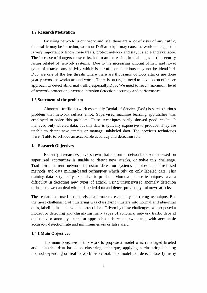
1.2 Research Motivation
By using network in our work and life, there are a lot of risks of any traffic,
this traffic may be intrusion, worm or DoS attack, it may cause network damage, so it
is very important to know these treats, protect network and stay it stable and available.
The increase of dangers these risks, led to an increasing in challenges of the security
issues related of network systems. Due to the increasing amount of new and novel
types of attacks, any activity which is harmful or malicious may not be identified.
DoS are one of the top threats where there are thousands of DoS attacks are done
yearly across networks around world. There is an urgent need to develop an effective
approach to detect abnormal traffic especially DoS. We need to reach maximum level
of network protection, increase intrusion detection accuracy and performance.
1.3 Statement of the problem
Abnormal traffic network especially Denial of Service (DoS) is such a serious
problem that network suffers a lot. Supervised machine learning approaches was
employed to solve this problem. These techniques partly showed good results. It
managed only labeled data, but this data is typically expensive to produce. They are
unable to detect new attacks or manage unlabeled data. The previous techniques
weren’t able to achieve an acceptable accuracy and detection rate.
1.4 Research Objectives
Recently, researches have shown that abnormal network detection based on
supervised approaches is unable to detect new attacks, or solve this challenge.
Traditional current network intrusion detection systems employ signature-based
methods and data mining-based techniques which rely on only labeled data. This
training data is typically expensive to produce. Moreover, these techniques have a
difficulty in detecting new types of attack. Using unsupervised anomaly detection
techniques we can deal with unlabelled data and detect previously unknown attacks.
The researchers used unsupervised approaches especially clustering technique. But
the most challenging of clustering was classifying clusters into normal and abnormal
ones, labeling instance with a correct label. Driven by these challenges, we proposed a
model for detecting and classifying many types of abnormal network traffic depend
on behavior anomaly detection approach to detect a new attack, with acceptable
accuracy, detection rate and minimum errors or false alert.
1.4.1 Main Objectives
The main objective of this work to propose a model which managed labeled
and unlabeled data based on clustering technique, applying a clustering labeling
method depending on real network behavioral. The model can detect, classify many

3
types of abnormal network traffic especially DoS with more effective accuracy and
detection rate.
1.4.2 Specific Objectives
There are many specific objectives included in main objectives:
Define the factors which help us to construct network behavior and can be
important for building our proposed model. This done by:
o Identifying abnormal network traffic, different types of abnormal
traffic, its classification, DoS, intrusion detection system, main types
and approaches,
o Definition of data mining, clustering technique, decision tree and
clusters validation measurements.
Using real network traffic behavior to be able to detect, estimate the behavior
of instance traffic and clustering label.
Developing clustering model based on anomaly behavior detection approach
using unsupervised learning machine technique to be able to classify traffic
data into normal or abnormal which help us to detect new attacks in the
system.
Labelling clusters and instances using proposed strategy based on special
criteria to classify these clusters into normal or abnormal classes.
Testing our proposed model on new unlabeled data to observe the system
ability to label, classify clusters and instances with correct class for using them
to detect new attacks.
Evaluation and calculation the performance measurements of proposed model,
accuracy and detection rate from the experimental results. Compare the results
with previous detection models.
1.5 Research Scope and Limitation
This research aims to propose a model which managed labeled and unlabeled data
based on clustering technique, applying a new clustering labeling method depending
on real network behavioral and nearest distance to detect, classify known/unknown
types of attacks. This research is applied with some limitations and assumptions such
as:
The proposed model used two types of DoS, Neptune and Smurf from KDD
Cup ‘99 datasets.

4
The proposed model used labeled dataset for training phase to learn model
about behavior of instance and label the clusters.
The proposed model used network based intrusion detection side, managed
network traffic within local network.
The proposed model used behavior-based IDS “anomaly detection approach”
that abnormal network traffic is necessarily differing from normal behavior.
The proposed model built network behavior rules depending on the size and
quality of training data. The extent of their representation of the majority of
the movements within the network.
1.6 Significant of the research
Add effective technique into abnormal detection solutions.
Construct effective model for detecting, classifying many types of abnormal
network traffic depend on behavior anomaly detection approach.
Help researchers who concern to predicate abnormal data in any field such as
abnormal data in informatics using clustering techniques and nearest distance.
Use a new clustering labeling approach which combined between more than
one technique to get more accuracy and zero false alert.
Help building more effective abnormal detection system which improves
intrusion detection system.
In the end, the result of the previous challenges to maintain network security and
system safer, a new model was proposed for detecting and classifying types of
abnormal network traffic especially DoS or a new attack based on clustering
technique. It depends on behavior anomaly detection approach to achieve acceptable
accuracy, detection rate and minimum errors or false alert.
1.7 Research Methodology
This research focused on DoS in abnormal detection based clustering to detect
known/unknown attacks or abnormal traffic. This was done by using unsupervised
approach with unlabeled data based on clustering technique. Applying a new
clustering labeling method depending on real network behavioral, to achieve more
effective accuracy, detection rate. There are many steps to perform the approach:

5
1.7.1 Research and Survey
In this step, we read, understand abnormal detection, DoS attack and main
detection techniques. Recent papers, books, articles, websites that are relative with
our problem were reviewed. Also previous researches were studied. The advantages
and disadvantages for each method were analyzed to overcome in our model.
1.7.2 Dataset collection, description and preprocessing
In this step, dataset was collected and used from [53]. The DARPA Intrusion
Detection Evaluation Program was prepared and managed by MIT Lincoln Labs. The
objective was to survey, evaluate research in intrusion detection. A standard set of
data to be audited, which includes a wide variety of intrusions simulated in a military
network environment, was provided. Lincoln Labs set up an environment to acquire
nine weeks of raw TCP dump data for a local-area network (LAN) simulating a
typical U.S. Air Force LAN. These dataset manipulated and processed according to
the need for it, we used codes tables to translate symbolic values into numeric and
vice versa.
1.7.3 Design and build the proposed model
In this step, the model was proposed and designed to solve abnormal detection
especially DoS problem by using data mining clustering technique based on real
network traffic. Chapter 4 depicts in details the proposed model.
1.7.4 Labeling clusters and new instances
In this step, a method was proposed to classify clusters into normal or
abnormal label using real network behavior and cluster size. Nearest distance was
used for determining labeling a new instance based on classified clusters. Chapter 4
depicts in details labelling method.
1.7.5 Applying and implementation the model
In this step, the proposed model was implemented using specific tools such as
RapidMiner [4] to represent clustering process. Oracle procedure was used for
implementation labeling processes.
1.7.6 Design experimental scenario
In this step, the model was verified using some of experimental cases. More
than one type of DoS were chosen, applied the model on the data sets. The used tools,
requirements and environments were explained.

6
1.7.7 Evaluation results of the model
In this step, the obtained results were analyzed and evaluated, also the
accuracy and detection rate were calculated. The results were compared with the
previous approaches results.
1.8 Outline of the Thesis
This thesis is divided into six chapters, which are structured around the
objectives of the research. The thesis was organized as follows:
Chapter 1, in this chapter, intrusion detection system, abnormal definition, main
goals for detection model, the research statement problem, objectives and outlines
were identified.
Chapter 2, in this chapter, literature review such as identifying anomalies, types and
characteristics were presented. Also intrusion detection techniques, machine learning,
data mining techniques, clustering and k-nearest neighbor techniques which used in
the model were defined.
Chapter 3, in this chapter, the related works which use machine leaning techniques
for detection abnormal network traffic and DoS attacks were presented and discussed.
Besides, the main advantages and shortages were highlight and discussed.
Chapter 4, in this chapter, the research proposal and methodology was presented.
The model architectures and scenarios were also presented. There is explanation about
our data sets used, dataset preprocessing, construct behavior rules, clustering process
and labeling method. There are baseline experiments to choose every parameter, tools
used in the model.
Chapters 5, in this chapter, the details of experiments were presented, analyzed the
results, discussed each experiment, and drew main figures and summaries.
Chapter 6, in this chapter, the conclusion and summary of the research achievement
of experiments were presented. Finally, future work was suggested.
7
1.9 Summary
In this chapter, intrusion detection system, abnormal definition, main goals for
detection model, the research statement problem, objectives and outlines were
identified and discussed. We proposed a model for detecting and classifying many
types of abnormal network traffic depend on behavior anomaly detection approach to
detect a new attack, with acceptable accuracy, detection rate and minimum errors or
false alert.

8
Chapter 2: Literature Review
In this chapter, anomalies, types, characteristics, intrusion detection
techniques, machine learning and data mining techniques were identified.
2.1 Anomalies Definition
Anomalies are patterns in data that do not conform to a well defined notion of
normal behavior, its goal is to monitor traffic and flag an alarm whenever some sort of
abnormal change happens. Several techniques have been proposed to address this
basic problem [6].
2.1.1 Types of Anomaly
An important aspect of an anomaly detection technique is the nature of the
desired anomaly. Anomalies can be classified into following three categories:
Point Anomalies: If an individual data instance can be considered as anomalous with
respect to the rest of data, then the instance is termed as a point anomaly. This is the
simplest type of anomaly and is the focus of majority of research on anomaly
detection. As a real life example, consider credit card fraud detection. Let the data set
correspond to an individual's credit card transactions. For the sake of simplicity, let us
assume that the data is defined using only one feature: amount spent. A transaction for
which the amount spent is very high compared to the normal range of expenditure for
that person will be a point anomaly [6].
Contextual Anomalies: If a data instance is anomalous in a specific context (but not
otherwise), then it is termed as a contextual anomaly (also referred to as conditional
anomaly). A temperature of 35F might be normal during the winter (at time t1) at that
place, but the same value during summer (at time t2) would be an anomaly [6].
Collective Anomalies: If a collection of related data instances is anomalous with
respect to the entire data set, it is termed as a collective anomaly. The individual data
instances in a collective anomaly may not be anomalies by themselves, but their
occurrence together as a collection is anomalous. Intrusion Detection System (IDS)
plays vital role of detecting various kinds of attacks or abnormal network traffic. The
main purpose of IDS is to find out intrusions among normal audit data and this can be
considered as classification problem [6]. Both of Point Anomalies and Collective
Anomalies are used in this research.
2.1.2 Anomalous Classification
Based on the flows responsible for a given anomaly, the anomaly can be
classified by looking at features like average packet sizes, application-level protocols,
number of sources and destinations, and so on. Anomalies involving many small

9
packets (e.g., TCP SYNs) usually indicate malicious traffic. The anomalies are
labeled as Denial-of-Service (DoS) attacks when one or more sources send many
small packets to a single destination. When one or more sources send small packets to
several destination ports of a single target host, we label it as a port scan. Other
anomalies are caused by applications that are unusual [7].
If we take record properties as criteria such as source IP, destination IP, source port,
destination port, transport protocol, flow size packet count, we can classify some of
attack according to them. Table 2.1 shows anomaly class and its description.
Table (2.1): Anomaly class and its description Anomaly class Description attack ICMP echo request and destination IP= broadcast smurf
flow size/packet count is too high ping-of-death
packet count = L, flow size= L ICMP flooding
TCP source IP = destination IP
source port=destination port
land
packet count = L, flow size= L TCP flooding
UDP destination port= reflecting port
source port= reflecting port
ping-pong
destination port= reflecting port
destination IP=broadcast
fraggle
packet count = L, flow size= L UDP flooding
For example, if the transport protocol is ICMP and its type is echo request and
destination is broadcast, then this flow is determined to be a smurf attack. The reason
is that the attack mainly sends spoofed source IP packets to the destinations of
broadcast. Ping-of-Death is attack flow by validating whether the length of the de-
fragmented packet is larger than the limited length that an IP packet can have.
In the case of a TCP transport protocol; this part certifies if the pair of source IP,
source port is identical with the pair of destination IP, destination port for the purpose
of detecting a Land attack.
In UDP flows, Fraggle and Ping-Pong attacks use UDP reflecting services, such as
echo (port 7).Therefore, the port numbers of source and destination port are validated.
If both destination and source ports are reflecting port numbers, then this flow is used
for the Ping-Pong attack. Also, if the destination port is a reflecting port and the
destination IP is a broadcast address, the flow is supposed to be a Fraggle attack,
similar to the Smurf attack [8].
DoS attacks are the main challenge in abnormal network traffic which used in this
research that consists of Neptune and Smurf attacks.
11
2.1.3 Denial of Service
Denial-of-Service (DoS) attack is one of the major threats in current computer
networks. It is an attempt to make a computer resource unavailable to the intended
users. This means to, motives for, and targets of a DoS attack may vary, but it
generally consists of the concerted, malevolent efforts of a person or persons to
prevent an internet site or service from functioning efficiently [66].
Denial of Service attack aims to bring legitimate users to experience a diminished
level of service or no service at all. Denial of Service is a frequent attack on the
Internet. An overview of how often a system is the target of a DoS attacks is given in
Moore et al [63]. The authors analyze multiple one-week traces covering over three
years from 2001 to 2004, and they conclude that on average each hour 24.5 different
IP addresses all over the world are the target of a DoS attack. The findings of Moore
et al. clearly show that DoS attack detection is, still in these days, a problem that
requires experts’ attention.
Neptune attack
The Neptune attack is a SYN-flood attack, which is a Denial-of-Service attack
that exploits a weakness of the TCP protocol. The first step of the three-way
handshake used to set up a TCP connection is to send a packet with the SYN flag set.
During a Neptune attack, massive amounts of such connection requests are sent to the
targeted machine. Each of these requests creates a half-open TCP connection on the
targeted machine, and information about this half-open connection is stored in
memory until a connection timeout occurs. The attacker’s aim is to exhaust the
memory available to store this information. If the attacker succeeds, the result is that
the system may crash or otherwise become unavailable for legitimate users [34].
Smurf attack
The Smurf attack utilizes the ICMP protocol and the internet infrastructure to
cause a Denial-of-Service attack. ICMP echo request packets are sent to the broadcast
address of different subnets, with the spoofed source address of the targeted
machine/network. By sending ICMP echo requests to the broadcast address, the
requests are amplified with the number of active host on the subnets. Each host on
these subnets will then issue an ICMP echo reply to the targeted machine. In worst
case, this means that a single ICMP echo request will cause that 255 ICMP echo
replies are sent to the targeted machine/network. If the attacker sends a stream of
ICMP echo request to various subnets, the amount of replies may exhaust the
resources of the targeted machine/network and render it unavailable for legitimate
users [34].

11
2.2 Intrusion detection system types
Intrusion detection approaches can be classified according to the monitoring
location as host-based or network-based (or a combination of both).
Network intrusion detection system (NIDS): is an independent platform that
identifies intrusions by examining network traffic and monitors multiple hosts,
developed in 1986 by Pete R. Network intrusion detection systems gain access to
network traffic by connecting to a network hub, network switch configured for port
mirroring, or network tap. In a NIDS, sensors are located at choke points in the
network to be monitored, often in the demilitarized zone or at network borders.
Sensors capture all network traffic and analyze the content of individual packets for
malicious traffic. An example of a NIDS is Snort [9].
Host-based intrusion detection system (HIDS): It consists of an agent on a host that
identifies intrusions by analyzing system calls, application logs, file-system
modifications (binaries, password files, capability databases, Access control lists, etc.)
and other host activities and state. In a HIDS, sensors usually consist of a software
agent. Some application-based IDS are also part of this category. Examples of HIDS
are Tripwire and OSSEC [9].
2.3 Intrusion Detection System Approaches
In addition to the monitoring location, intrusion detection techniques can be
classified according to the approach for data analysis to recognize anomalies. The two
basic approaches to data analysis are misuse detection and anomaly detection (which
can be combined):
Misuse detection approach defines a set of attack “signatures” and looks for
behavior that matches one of the signatures (hence this approach is sometimes called
signature-based IDS). This approach is commonly used in commercial IDS products.
Although the concept sounds simple, the approach involves more than simple pattern
matching; the most capable analysis engines are able to understand the full protocol
stack and perform stateful monitoring of communication sessions.
However, this approach is obviously dependent on the accuracy of the signatures. If
the signatures are too narrowly defined, some attacks might not be detected; these
cases of failed detection are false negatives. On the other hand, if signatures are too
broadly defined, some benign behavior might be mistaken for suspicious; these false
alarms are false positives. Signatures should be defined to minimize both false
negatives and false positives. In any case, misuse detection would not be able to
detect new attacks that do not match a known signature. These failures increase the
rate of false negatives. Since new attacks are constantly being discovered, misuse

12
detection has the risk of becoming outdated unless signatures are updated frequently
[10] [11].
Anomaly detection approach defines a statistical pattern for “normal” behavior, and
any deviations from the pattern are interpreted as suspicious. This approach has two
major drawbacks. First, it has been common experience that an accurate definition of
normal behavior is a difficult problem. Second, all deviations from normal behavior is
classified as suspicious or abnormal, but only a small fraction of suspicious cases may
truly represent an attack. Thus anomaly detection could result in a high rate of false
positives if every suspicious case raised an alarm. To reduce the number of false
alarms, additional analysis would be needed to identify the occurrences of actual
attacks. The main advantage of this approach is the potential to detect new attacks
without a known signature [10] [11].
Numbers of anomaly detection systems are developed based on many different
machine learning techniques and data mining.
2.4 Machine Learning
Machine learning is a branch of artificial intelligence, is a scientific discipline
concerned with the design and development of algorithms that take as input empirical
data, such as that from sensors or databases, and yield patterns or predictions thought
to be features of the underlying mechanism that generated the data. A learner can take
advantage of examples (data) to capture characteristics of interest of their unknown
underlying probability distribution. Data can be seen as instances of the possible
relations between observed variables. Machine learning algorithms can be organized
into two methods [12]:
Supervised Methods: The main goal of the supervised methods is to build a
predictive model (classifier) to classify or label incoming patterns. The classifier has
to be trained with labeled patterns to be able to classify new unlabeled patterns. The
given labeled training patterns are use to learn the description of classes. Some
supervised methods include support vector machines, neural network and genetic
algorithms among others [12].
Unsupervised Methods: Unsupervised methods take a different approach by
grouping unlabeled patterns into clusters based on similarities. Patterns within the
same clusters are more similar to each other than they are to patterns belonging to
different clusters. Data clustering is very useful when little priori information about
the data is available [12].

13
2.5 Data Mining It is non-trivial process of identifying valid, novel, potentially useful, and
ultimately understandable patterns in data. Also, it is the process of extracting
knowledge hidden from large volumes of raw data. The knowledge must be new, not
obvious, and must be able to use it. Many people treat data mining as a synonym for
another popularly used term, Knowledge Discovery from Data, or KDD.
Alternatively, others view data mining as simply an essential step in the process of
knowledge discovery [5].
Knowledge discovery as a process is depicted in Figure 2.1 and consists of an
iterative sequence of data mining steps as the following steps:
Data cleaning: to remove noise and inconsistent data.
Data integration: where multiple data sources may be combined.
Data selection: where data relevant to the analysis task are retrieved from the
database.
Data transformation: where data are transformed or consolidated into forms
appropriate for mining by performing summary or aggregation operations, for
instance.
Data mining: an essential process where intelligent methods are applied in
order to extract data patterns.
Pattern evaluation: to identify the truly interesting patterns representing
knowledge based on some interestingness measures.
Knowledge presentation: where visualization and knowledge representation
techniques are used to present the mined knowledge to the user [5].

14
Figure (2.1): Data mining as a step in the process of knowledge discovery [5].
15
2.5.1 Data Mining Tasks
Data mining tasks can be classified into two categories: The first are
Descriptive mining tasks characterize the general properties of the data. Second are
Predictive mining tasks performing inferences on the current data in order to make
predictions. The most famous data mining tasks [20]:
Classification [Predictive]: used for predictive mining tasks. The input data for
predictive modeling consists of two types of variables: First explanatory variables,
which define the essential properties of the data, and the second is one target
variables, whose values are to be predicted. Classification is used to predicate the
value of discrete target variable. Decision Tree and Rule Induction are almost famous
samples.
Prediction [Predictive]: Similar to classification, except we are trying to predict the
value of a variable.
Association Rules [Descriptive]: seek to produce a set of rules describing the set of
features that are strongly related to each others.
Clustering [Descriptive]: Find groups of data pointes (clusters) so that data points
that belong to one cluster are more similar to each other than to data points belonging
to different cluster.
Outlier Analysis [Predictive]: Discovers data points that are significantly different
than the rest of the data. Such points are known as anomalies or outliers [20].
2.6 Clustering
Clustering is an unsupervised learning technique which divides the datasets
into subparts, which share common properties. For clustering data points, there should
be high intra cluster similarity and low inter cluster similarity. A clustering method
which results in such type of clusters is considered as good clustering algorithm.
Clustering algorithms can be classified according to the method adopted to define the
individual clusters. The algorithms can be broadly classified into the following types:
partitional clustering, hierarchical clustering, density-based clustering and grid-based
clustering [14]. These algorithms are based on distance measure between two objects.
Basically the goal is to minimize the distance of every object from the center of the
cluster to which the object belongs [13] [29].
2.6.1 Clustering Classification Methods:
The process of grouping a set of physical or abstract objects into classes of
similar objects is called clustering. There are four main types for clustering
classification:

16
Partitional clustering: Partition-based methods construct the clusters by creating
various partitions of the dataset. So, partition gives for each data object the cluster
index pi. The user provides the desired number of clusters M, and some criterion
function is used in order to evaluate the proposed partition or the solution. This
measure of quality could be the average distance between clusters; for instance, some
well-known algorithms under this category are k-means, PAM and CLARA [15] [16].
One of the most popular and widely studied clustering methods for objects in
Euclidean space is called K-Means clustering. Given a set of N data objects xi and an
integer M number of clusters. The problem is to determine C, which is a set of M
cluster representatives cj, as to minimize the mean squared Euclidean distance from
each data object to its nearest centroid. The number of iterations depends upon the
dataset, and upon the quality of initial clustering data. The k-means algorithm is very
simple and reasonably effective in most cases. Completely different final clusters can
arise from differences in the initial randomly chosen cluster centers. In final clusters
k-means do not represent global minimum and it gets as a result the first local
minimum [13][29].
Hierarchical clustering: Hierarchical clustering methods build a cluster hierarchy,
i.e. a tree of clusters also known as dendogram. A dendrogram is a tree diagram often
used to represent the results of a cluster analysis. Hierarchical clustering methods are
categorized into agglomerative (bottom-up) and divisive (top-down). An
agglomerative clustering starts with one-point clusters and recursively merges two or
more most appropriate clusters. In contrast, a divisive clustering starts with one
cluster of all data points and recursively splits into non overlapping clusters [13][29].
Hierarchical methods provide ease of handling of any form of similarity or distance,
because use distance matrix as clustering criteria. However, most hierarchical
algorithms do not improve intermediate clusters after their construction. Furthermore,
the termination condition has to be specified. Hierarchical clustering Algorithms
include BIRCH [17] and CURE [18].
Density-based clustering: The key idea of density-based methods is that for each
object of a cluster the neighborhood of a given radius has to contain a certain number
of objects; i. e. the density in the neighborhood has to exceed some threshold. The
shape of a neighborhood is determined by the choice of a distance function for two
objects. These algorithms can efficiently separate noise [19]. DBSCAN [20] and
DBCLASD [21] are the well-known methods in the density based category.
Grid-based clustering: The basic concept of grid-based clustering algorithms is that
they quantize the space into a finite number of cells that form a grid structure. And
then these algorithms do all the operations on the quantized space. The main
advantage of the approach is its fast processing time, which is typically independent
of the number of objects, and depends only on the number of grid cells for each

17
dimension [14]. Famous methods in this clustering category are STING [22] and
CLIQUE [23].
Other techniques available include model-based clustering, constraint-based and
fuzzy clustering [24]. Model-based methods hypothesize a model for each of the
clusters and find the best fit of that model to each other. One method from this
category is EM algorithm [25]. The idea of constraint-based clustering is finding
clusters that satisfy user specified constraints, for example as in COD CLARANS
method [26]. Fuzzy clustering methods attempt to find the most characteristic objects
in each cluster, which can be considered as the center of the cluster, and then, find the
membership for each object in the cluster. A common fuzzy clustering algorithm is
Fuzzy C-Means [27].
Partitional Clustering (K-Means) was used in the model for choosing cluster
technique based on practical experiments.
2.6.2 Clustering application
Clustering problems are widely used in numerous applications, such as
customer segmentation, classification, and trend analysis. For example, consider a
retail database records containing items purchased by customers. A clustering
procedure could group the customers in such a way that customers with similar
buying patterns are in the same cluster. Many real-word applications deal with high
dimensional data. It has always been a challenge for clustering algorithms because of
the manual processing is practically impossible. A high quality computer-based
clustering removes the unimportant features and replaces the original set by a smaller
representative set of data objects. As a result, the size of data reduces and, therefore,
cluster analysis can contribute in compression of the information included in data.
Cluster analysis is applied for prediction. Suppose, for example, that the cluster
analysis is applied to a dataset concerning patients infected by the same disease. The
result is a number of clusters of patients, according to their reaction to specific drugs.
So, for a new patient, we identify the cluster in which he can be classified and based
on this decision his medication can be made [27] [28].
2.6.3 Clustering Problems
The general clustering problem includes three problems [13]: Selection of the
evaluation function, decision of the number of groups in the clustering and the choice
of the clustering algorithm.
Evaluation of clustering: An objective function is used for evaluation of clustering
methods. The choice of the function depends upon the application, and there is no
universal solution of which measure should be used.

18
Commonly used a basic objective function is defined as Eq. (2.1).
Where P is partition and C is the cluster
representatives, d is a distance function. (2.1)
The Euclidean distance and Manhattan distance are well-known methods for distance
measurement, which are used in clustering context. Euclidean distance is expressed as
Eq. (2.2).
Euclidean distance (2.2)
Number of clusters: The choice of number of the clusters is an important sub
problem of clustering. Since a priori knowledge is generally not available and the
vectors dimensions are often higher than two, which do not have visually apparent
clusters. The solution of this problem directly affects the quality of the result. If the
number of clusters is too small, different objects in data will not be separated.
Moreover, if this estimated number is too large, relatively regions may be separated
into a number of smaller regions. Both of these situations are to be avoided. This
problem is known as the cluster validation problem. The aim is to estimate the
number of clusters during the clustering process. The basic idea is the evaluation of a
clustering structure by generating several clustering for various number of clusters
and compare them against some evaluation criteria [31] [32].
In general, there are three approaches to investigate cluster validity. In external
approach, the clustering result can be compared to an independent partition of the data
built according to our intuition of the structure of the dataset. The internal criteria
approach uses some quantities or features inherent in the dataset to evaluate the result.
The basic idea of the third approach, relative criteria, is the evaluation of a clustering
structure by comparing it to other clustering schemes, produced by the same
algorithm but with different input parameter values. The two first approaches are
based on statistical tests and their major drawback is their high computational cost. In
the third approach aim is to find the best clustering scheme that a clustering algorithm
can define under certain assumptions and parameters. More information about
clustering validity methods you can find in [31] [32].
The choice of the clustering algorithm: The K-means algorithm, a hard partitional
clustering algorithm, was chosen for its simplicity and speed with the Euclidean
metric as the similarity measure. The general steps for the K-means algorithm were
the following:
Chose number of clusters (K).
Initialize centroids (K patterns randomly chosen from data set).

19
Assign each pattern to the cluster with closest centroid.
Calculate means of each cluster to be its new centroid.
Repeat step 3 until a stopping criteria are met (no pattern move to another
cluster).
This procedure was repeated 10 times and the best clustering solution was
chosen.
The following Figure 2.2 is an example that shows how the centroids changed
position and how the samples are assigned to different clusters for several iterations of
the K-Means algorithm [30] [33].
Figure (2.2): K-Means output for different iterations
2.6.4 Clustering quality indexes
Clustering quality indexes have been used so far to tell us how well the data
has been grouped into clusters, e.g. in algorithms used to find the optimal number of
clusters for partitional clustering algorithms. There are several quality indexes
available, for example the Davies-Bouldin index, the Silhouette index, Dunn’s index
and the C index. In this section we give a brief summary of how these indexes are
computed, and which cluster parameters are used to evaluate the clustering quality
[34] [35] [36].
The Davies-Bouldin index is defined by the following formula [35]:
Parameters used in the Davies-Bouldin index, to evaluate the quality of the clustering,
are the total of the average intra-cluster distances and the average inter-cluster
distances. In the formula, M is the number of clusters, d is the average distance
between the entities within the cluster and the cluster center c, and d(..) is the distance
between the clusters.

21
The output from the Davies-Bouldin formula is a value between 0 and 1. We have
good clustering when a cluster is compact and the different clusters are distant from
each other. In such cases the value of the Davies-Bouldin index is low [57] [69].
The Silhouette index uses the Silhouette width of each entity in a cluster to evaluate
the clustering quality. This width is the confidence indicator of the entities’
membership of a cluster. To compute this width, the minimum average distance to
entities in other clusters is used, as well as the average distance to all other entities in
the same cluster. To normalize this result, the maximum of the two distances is used.
Computation of the Silhouette width yields a value between -1 and 1. A value near 1
indicates that the entity is within the correct cluster, a value near 0 means that the
entity could also be a part of another cluster, while a value near -1 indicates that the
entity has been placed in a wrong cluster. The Silhouette width of a cluster is the
average sum of the silhouette widths of the entities within the cluster, and the
Silhouette index of the entire clustering is the average sum of all cluster Silhouette
widths[57] [69].
The following formulas are used to compute the Silhouette index [35]:
where aji is the average distance between entity i and the other entities in the cluster,
and bji is the minimum average distance to entities in other clusters. We can then find
the silhouette width for a cluster by:
Where m is the number of entities.
Dunn’s index only measures two parameters and the index is defined by the
following formula [35]:
The parameters used to evaluate the clustering with Dunn’s index are the minimum
inter-cluster distance and the maximum intra-cluster distance. In this formula, c is the
number of clusters, D is the average distance between the entities within the cluster
and the cluster center c, and d(..) is the distance between the clusters. Because the
index only measures two parameters, it may not yield stable results in some situations,
e.g. when there are so-called outliers in the clustered data set.
On the other hand, it can be computed quite fast, which is important for the efficiency
of our labelling strategy. The two parameters used to compute this index are the
minimum inter-cluster distance between clusters and the maximum intra-cluster

21
distance. This is better illustrated by the simplified formula for Dunn’s index, given
by Gunter et al. [36]:
In this formula, dmin is the minimum inter-cluster distance and dmax in the maximum
intra-cluster distance. Good clustering means that the inter-cluster distance is high and
the intra-cluster distance is low. Higher values of the Dunn’s index therefore indicate
good clustering quality.
2.9 K-Nearest Neighbors
The k-nearest neighbors’ (k-NN) algorithm is a method for classifying objects
based on closest training examples in the feature space. K-NN is a type of instance-
based learning, or lazy learning where the function is only approximated locally and
all computation is deferred until classification. The k-nearest neighbor algorithm is
amongst the simplest of all machine learning algorithms: an object is classified by a
majority vote of its neighbors, with the object being assigned to the class most
common amongst its k nearest neighbors (k is a positive integer, typically small). If k
= 1, then the object is simply assigned to the class of its nearest neighbor [74].
2.10 Abnormal Network Traffic Detection Goals
To protect networks from abnormal network traffic especially DoS, reach
maximum network security and protect from theft or damage.
To achieve a model for detecting and classifying many types of abnormal
network traffic, besides helping to detect new types of attacks in network
traffic, improve intrusion detection alert system.
To overcome the shortage of traditional and supervised abnormal detection
approaches, increase the system accuracy and detection rate.
To overcome the shortage of traditional labeling clusters for approaches that
used clustering techniques and classify data into normal or abnormal.
To improve abnormal traffic detection rate and reduce false detection alarm.
To construct a new technique of combination of more than one technique for
detection abnormal traffic with labeling clusters to achieve acceptance
accuracy and detection rate.
To construct a generalization model that can be used for detecting
normal/abnormal traffic, worm and intrusion.

22
2.11 Summary
In this chapter, anomalies, types, characteristics, intrusion detection
techniques, machine learning and data mining techniques were identified. Network
traffic detection goals were discussed. In addition, main problems for clustering were
discussed. Traditional clustering such as k-means and k-nearest neighbor were
identified and discussed for using them in the model.
23
Chapter 3: Related work
This chapter introduces the state of the art for the applied techniques in
abnormal detection in some domains. This chapter introduces the state-of the art for
the applied techniques in intrusion detection in some domains and addressing various
technologies used in intrusion detection systems. The chapter is addressing various
technologies used in intrusion detection which based on cluster size, distance metrics
and outlier, fuzzy clustering and classification techniques. Finally, the weak points of
the related works were presented and discussed.
3.1 Abnormal detection based on cluster size
Portony et-al [40] presented a method for clustering similar data instances together
and uses distance metrics on clusters to determine an anomaly. The author makes two
basic assumptions: First, data instances having the same classification should be
closed to each other in feature space under some reasonable metric, while instances
with different classifications should be far apart. Second, the number of instances in
the training set that represent normal traffic is overwhelmingly larger than the number
of intrusion instances. Clusters were labeled based on cluster size; the biggest cluster
(>98%) will be labeled as normal and others as abnormal.
The solution is able to detect new types of intrusion while maintaining a low false
positive rate. Their method is effective when almost network traffic is normal class
and homogenous, but the problem of this solution is that they depend on one
technique ‘size’, may be not accurate in DoS attack, almost data is abnormal, the big
cluster (actually abnormal) will be considered as normal. Also if any assumption
doesn’t achieve its criteria, the system accuracy will decrease and give high false
alert.
Bhuyan et-al [42] used a new solution which detects network anomalies using an
unsupervised approach with minimum false alarms. First, they introduce a tree based
subspace clustering technique (TreeCLUS) for generating clusters in high
dimensional large datasets. TreeCLUS exploits a specific technique for finding a
highly relevant feature set. Second, they analyze the stability of the cluster results
obtained. Third, they propose a cluster labeling technique (CLUSLab) to label the
stable clusters using a multi-objective approach using cluster size, compactness and
dominating feature subset. The solution used multi approaches for labeling the
clusters; it will decrease false alarm, while increase the percent of detection rate. The
problem in this solution is that stability of cluster is not exclusive in normal clusters,
but also in abnormal clusters such as DoS. In addition, they didn’t determine the
techniques that have been used for choosing relative features.
Borah et-al [60] proposed a behavior model for normal and attack instances. A
subspace based incremental clustering technique with proper outlier handling
24
capability is used to cluster the dataset in which anomaly detection need to be
performed. The parameters of the clustering algorithm are tuned to detect clusters
reflecting the behavioral proposed model. Based upon the clustering results records
could be labeled as normal and anomalous. Attributes with continuous values are
discredited before applying the categorical clustering algorithm. Algorithm works
based on two principles. First, the clustering algorithm should be able to distinguish
minor differences between normal and attack instances so that as far as possible pure
clusters are formed with only one kind of instances - either attack or normal.
Secondly, besides cluster sizes some other criteria need to be used for labeling
clusters. The assumptions used for detecting anomalies are; first some attacks are
similar over very large subspaces, other attacks are similar over smaller subspaces or
have lower occurrences. Second normal records are similar over medium sized
subspaces. The problem of this solution is that they use cluster size (incremental
algorithm) and outlier for labeling the cluster, based on attacks form smaller
subspaces which will represent outliers. This technique could not process massive
attack or DoS, also there is no specific method to label clusters and managing new
instance after detection abnormal.
Chimphlee et-al [50] presented anomaly detection method that used clustering
technique on unlabeled data according clustering width they Labeled clusters Some
percentage N of the clusters containing the largest number of instances associate with
them as ‘normal’. They process any instance after conversion, they found a cluster C
which is closest to d′ under the metric M, Classify d′ according to the label of C
(normal or anomalous). The method is able to detect many different types of
intrusions, while maintaining a low false positive rate as verified over the clustering
on KDD CUP 1999 dataset. The problem is that the solution depends on cluster width
or size for detection process. They assume that the largest number of instances is
associated with them as ‘normal’. This gives a high false alarm in DoS case which
abnormal data may be the largest cluster.
Nieves et-al [52] presented anomaly detection method that used a simple clustering
algorithm over the Kdd Cup 1999 network data set. They used Cluto data clustering
software, was used with the Kmeans algorithm to cluster the data. Then, the labeling
procedure of the clusters was done based cluster size and number of clusters Based on
their assumption that a real network contains many more normal connections than
attacks, the smaller clusters are consider to contains attacks and the bigger clusters are
consider to contains normal or good connections. The clustering procedure was done
for 10, 20 and 30 clusters (K), they found that increasing the total number of clusters
(K) help to achieve a higher detection rate while maintaining a low false alarm rate.
More pure clusters mean that they have more attacks and fewer amounts of normal
connection in the smaller clusters and more normal connections and fewer amounts of
attacks in the bigger clusters.
25
Their system proved that using data clustering methods for anomaly detection in
network intrusion detection may achieve a high detection rate of attacks (including
previously unseen attacks) while maintaining a low false alarm rate without the need
of going through the labeling procedure. Also results of the evaluation confirm that a
high detection rate can be achieved while maintaining a low false alarm rate. The
problem is that the number of clusters is determined manually. They assume that the
small clusters are considered as attacks, while the big clusters are normal. In DoS
case, the false alarm will be increased due to previous assumption.
3.2 Abnormal detection based on distance metrics and outlier
Jayasimhan et-al [43] proposed system for detection abnormal which uses selection
features as preprocessing, then create clusters based on k-means, then classify data
according to distance into normal or abnormal and if instance is near into normal then
it is normal, else abnormal. They applied their model on DARPA KDD dataset which
split into training and testing, the features of network traffic were classified into three
types; basic features, content features and traffic features. They construct pattern
detection using clustering, they assume number of clusters is 2 consists of normal and
abnormal. This solution is simple retrieve good result, using good and efficient
technique for clustering.
In this solution, K-Means was used for clustering technique to identify and detect
novel attacks. Also it reduced the false negative rate. The problem of this system is
that labeling clusters method is not discussed. The number of clusters has to be
determined manually at the beginning of the process. They assume that the model has
only two clusters; this assumption is not existed in real system. The model
performance such as detection rate and accuracy wasn’t calculated.
Burbeck et-al [61] presented anomaly detection method that used the first phase of
the existing BIRCH clustering (BIRCH: balanced iterative reducing and clustering
using hierarchies) framework to implement fast, scalable and adaptive anomaly
detection. It uses training data assumed to consist only of normal data to construct the
tree. After being trained, it is used to detect anomalies in unknown data. When a new
data point arrives detection starts with a top down search from the root to find the
closest cluster feature. When search is done, the distance from the centroid of the
cluster to the new data point is computed. The new data point is considered normal if
the distance is lower than a limit otherwise it is an anomaly. The number of alarms is
then further reduced by application of an aggregation technique. Some normal types
of system activities might produce limited amounts of data, but still be desirable to
incorporate into the detection model since detection is not based on cluster sizes.
Their experiments show a good detection quality (95 %) and acceptable false
positives rate (2.8 %) considering the online, real-time characteristics of the
algorithm.
26
Chandola et-al [45] presents methods for anomalies detection using clustering
technique; they suppose that there are three cases: first, normal data instances belong
to a cluster in the data, while anomalies either do not belong to any cluster. Second,
normal data instances lie close to their closest cluster centroid, while anomalies are far
away from their closest cluster centroid. Third, normal data instances belong to large
and dense clusters, while anomalies either belong to small or sparse clusters. This
solution can classify many of abnormal cases, but the problem is that some cases data
may be out of those ranges or classes. The accuracy and efficiency were not
discussed. Moreover, the criteria (distance, outlier and the size) of the system couldn’t
determine all the cases of abnormal especially DoS.
Gupta et-al [2] presented a new approach that combines specification-based and
anomaly-based intrusion detection, mitigating the weaknesses of the two approaches
while magnifying their strengths. The approach begins with state-machine
specifications of network protocols, and augments these state machines with
information about statistics that need to be maintained to detect anomalies. They
present a specification language in which all of this information can be captured in a
succinct manner. They demonstrate the effectiveness of the approach on the 1999
Lincoln Labs intrusion detection evaluation data, where we are able to detect all of the
probing and denial-of-service attacks with a low rate of false alarms (less than 10 per
day). Whereas feature selection was a crucial step that required a great deal of
expertise and insight in the case of previous anomaly detection approaches. Moreover,
the machine learning component of their approach is robust enough to operate without
human supervision and fast enough that no sampling techniques need to be employed.
Also present results of applying their approach to detect stealthy email viruses in an
intranet environment.
Leung et-al [1] proposed a density based and grid based clustering algorithm, named
as fpMAFIA, that uses adaptive grid algorithm adopted from pMAFIA and FP-tree
growth method for frequent item set mining. They aim to discover clusters from large
volume of high dimensional input data. It is an optimized version of the original
pMAFIA algorithm, with the modification that they use the Frequency-Pattern Tree
(FP-Tree) in the intermediate step. Grid-based methods divide the object space into a
finite number of cells that form a grid structure. All of the clustering operations are
performed on the grid structure. Once they obtain the set of clusters, they expect that
they cover most but not all of the data set. Therefore any point that falls inside the
clusters will be labeled as normal. The small percentages of points that do not belong
to any clusters are labeled as abnormal. The main advantage of this approach is its fast
processing time, which is typically dependent mainly on the number of cells in each
dimension in the quantized space. pMAFIA is an optimized and improved version of
CLIQUE. But pMAFIA used the adaptive grid algorithm to reduce the total number of

27
potential dense units by merging small 1-dimensional partitions that have similar
densities. Also, it parallelized the operation of the generation and population of the
candidate dense units using a computer cluster. However, they both scale
exponentially to the dimension of the cluster of the highest dimension in the data set.
Their implementation of fpMAFIA is able to run with a large data set of 1 million
records on a single PC and terminates in less than 11 minutes.
Their solution has the advantage that it can produce clusters of any arbitrary shapes
and cover over 95% of the data set with appropriate values of parameters. They
provided a detailed complexity analysis and showed that it scales linearly with the
number of records in the data set. They have evaluated the accuracy of the new
approach and showed that it achieves a reasonable detection rate while maintaining a
low positive rate.
The problem is that they consider the large cluster as normal, but if there is any
difference or changes in this assumption, the accuracy will be decreased and system
will give high false alert. In addition, they assume a small percentage of points that do
not belong with any clusters are labeled as abnormal, but in the real network this is
not always true, all points must belong the clusters.
Malik et-al [51] proposed an Adaptive network intrusion detection system (NIDS)
using K-Means clustering techniques. Definite behavior of network traffic is precisely
captured using Data mining approaches, and the set excavated differentiates between
“normal” and “attack” traffic. Proposed system was constructed by a number of
Agents, which are totally different in both training and detecting processes. The
proposed NIDS is composed of four modules, feature miner, Anomaly based agents,
signature based agent and agent trainers. First, a feature extractor converts the data
from monitored system into features which will be used in both training and network
intrusion detection stages. Using k-means clustering algorithm, respective type of
packets is clustered under respective Agents formed after clustering. Each of the
Agents is responsible for capturing a network behavior type and hence the system has
strength on detecting different types of attacks as well as ability of detecting new
types of attacks. They used K-means to find how far (Euclidean distance) of a
candidate cluster from normal. If the distance is larger than a threshold, the cluster
will be regarded as an intrusion, or vice versa. An anomaly detection model is based
on normal behavior only and deviations from it. In other words, the normal behavior
of the network is profiled. They used Number of Unique ports accessed, Mean Packet
Size, Time to live and Window size for agent to detect the behavior.
Their experimental results showed that the network traffic pattern used as reliable
agents outperforms from traditional signature-based NIDS. The problem in this model
is they determine number of cluster manually; also possibly high in false alarm rate as
previously system behaviors may be recognized as anomalies.

28
3.3 Abnormal detection based on fuzzy clustering
Hameed et-al [47] proposed an algorithm for intrusion detection that combines both
fuzzy C Means (FCM) and FCM for symbolic features algorithms in one. In order to
manipulate with network traffic data stream that contains symbolic features in
addition to the numeric features, the proposed algorithm combines both the
conventional FCM algorithm that partitions only the numeric features patterns and
FCM that partitions symbolic features in one algorithm. The most known method of
fuzzy clustering is the FCM. FCM is a method of clustering which allows one piece of
data to belong to two or more clusters. This method was proposed by Dunn in 1973.
The proposed algorithm uses 33 features from KDD cup 99 instead of 41 features.
Also, the proposed algorithm gives better result than conventional FCM and FCM for
symbolic features. The average detection rate of the proposed algorithm was 99 which
out performs the average DR of algorithms C5.4 and ID3 that have average DR is
98.3 and 92.1 respectively. Experimental results on KDDcup99 intrusion detection
dataset show that the average detection rate of this algorithm is 99%. The results
indicate that the proposed algorithm is able to distinguish between normal and attack
behaviors with high detection rate. The problem of this solution is that there is no
obvious pattern for detection abnormal traffic, also there is no a specific method to
label the clusters and managing a new instance after detection abnormal.
Chimphlee et-al [49] proposed an intrusion detection method that combines Rough
set and Fuzzy Clustering. Rough set has to decrease the amount of data and get rid of
redundancy. Fuzzy c-means clustering allow objects to belong to several clusters
simultaneously, with different degrees of membership. The model begin with
preprocessing by using misusing or incomplete data preprocessing, then they reduce
data dimension using rought set were done by Rosetta software that used to select
attributes, final they clustering data using Fuzzy c-means clustering technique, they
determine number of cluster manually, assume k=5.
The approach allows to recognize not only known attacks, but also to detect
suspicious activity that may be the result of a new unknown attack. The problem of
this model is that the number of clusters is determined manually (k=5). The method of
detecting the attacks is not covered. In addition, the experimental results, the detection
rate and the accuracy aren’t calculated.
Xie et-al [59] proposed an anomaly detection method that the fuzzy C-means
clustering (FCM) algorithm was applied to detect abnormality which based on
network flow. The method combined with the average information entropy, support
vector machine and fuzzy genetic algorithm. These hybrid algorithms can solve the
mentioned problems and classify more accurately. They improved intrusion detection
algorithm based on FCM, by using three steps; first they initialized the membership
matrix U with random number between 0 and 1, after that they calculated the cluster
29
centers; finally they calculated the new membership matrix U. The problem of this
model is that they don’t use any method to label clusters (doesn't covered). There are
no experiments for the model. The detection rate and accuracy are not calculated.
Zhong et al. [56] propose an approach that does not use any historical training data,
which only use the observed activities to obtain the clusters. The authors investigate
four clustering techniques for use in intrusion detection. For labelling, they use inter-
and intra-cluster distances for labelling. The largest cluster is assumed to be normal,
and then other clusters are sorted by the distance from that clusters’ centroid to the
centroid of the largest cluster. The entities within each cluster are sorted in the same
way, by their distance to the centroid of the largest cluster. A given or estimated
number of those entities, with the shortest distance to the centroid, are then labeled
normal and the remaining entities are labeled as attacks. Their results show that
clustering is suitable for intrusion detection, and that the performance of clustering
based IDSs is comparable with traditional approaches. They showed that combining
traditional techniques with clustering techniques can increase the performance of IDS.
The results also confirm the authors’ hypothesis that clustering is better suited for
detecting previously unknown attacks than traditional approaches. The problem of
this solution is that the largest cluster is considered as normal, when normal data
transmitted by means of a less frequently used protocol (such as ftp or telnet) might
produce small clusters, which could increase the false alarm.
Jiang et-al [44] proposed a new strategy for intrusion detection. It consists of three
stages, based on clustering training data, then sort clusters according to their outlier
factor. Then label some clusters that contain percentage e of the data as ‘normal’
while labeling the rest of the clusters as ‘attack’. They regard labeled clusters as
model, and detect an object whether it is an attack or not by the distance between an
object and the nearest cluster. They considered the outlier factor of clusters for
measuring the deviation degree of a cluster. A novel method has been proposed to
compute the cluster radius threshold. The data classification has been performed by an
improved nearest neighbor method. The experiments demonstrated that their method
outperforms the existing methods in terms of accuracy and detecting unknown
intrusions. This solution is effective when almost data in the network is a normal. It
depends on outlier factor and may be changed according to its threshold.
Thiprungsri et-al [48] proposed a anomaly detection procedure which start with
normalize the attributes and perform preprocessing dataset, then they used k-means
for clustering and calculation cluster centroid and each observation is assigned to the
closet cluster. The next step, computes the distance between each observation and the
cluster centers. If the observation is not currently a member of the cluster with the
closet centroid, the observation is reassigned to a new cluster. The former cluster
loses membership, while the new cluster with the closet centriod gains membership.
The centroid recalculated. The process from step three repeats until there is no new
31
assignment. The model use outlier as main criteria for detection anomaly, after
calculated the distances. The problem is that there is no experimental results in output,
also the method of detecting the attacks and calculating the detection rate is not
discussed. Labeling clusters is one challenge in the system.
3.3 Abnormal detection based on classification techniques
Purohit et-al [41] proposed a model which is the combination of three different
techniques K-Mean clustering, Naive Bayes (statistical) and Decision Table Majority
(rule based) approaches. For the first stage in the proposed hybrid IDS model, they
group similar data instances based on their behaviors by using a K-Means clustering
as a pre-classification component. For the second stage, they used Naïve Bayes
classifier which classifies the resulting clusters into classes like normal and abnormal.
System data that has been misclassified during the earlier stage may be correctly
classified in the subsequent classification stage. The problem of this system is that
labeling clusters method is not investigated. The performance of the model such as
detection rate and accuracy isn’t calculated.
Panda et-al [70] presents a methodology to recognize attacks during the normal
activities in a system. A novel classification via sequential information bottleneck
(sIB) clustering algorithm has been proposed to build an efficient anomaly based
network intrusion detection model. They have compared their method with other
clustering algorithms like X-Means, Farthest First, Filtered clusters, DBSCAN,K-
Means clustering in order to find the suitability of their proposed algorithm. The
results show that the proposed method is efficient in terms of detection accuracy, low
false positive rate. They design a simple meta-classifier that uses a clusterer for
classification, for cluster algorithms that use a fixed number of clusterer, like Simple
K-Means, the user has to make sure that the number of clusters to generate is the same
as the number of class labels in the dataset in order to obtain a useful model. Then,
they proposed Sequential Information Bottleneck Clustering (sIB) which consists of
four steps. The detection rate of the model is 86.3. They need to increase this value.
Also they determine the number of clusters manually.
Upadhyaya et-al [71] proposes a hybrid approach which is the combination of
K-Medoids clustering and Naïve-Bayes classification for intrusion detection and how
it is useful for IDS. The proposed approach applies clustering on all data into the
corresponding group and after that applies a classifier for classification purpose.
Naïve Bayes Classification can be mined to find the abstract correlation among
different security features. The proposed hybrid IDS is divided into following module:
Database Creation which consists of selecting and generating the data source data
scope transformation and preprocessing, Data Mining techniques which uses K-
Medoids cluster technique, also Naïve Bayes classification and the calculation of the
performance. The Proposed system gives less false alarm rate, faster than existing

31
system in terms of execution time, smaller than the existing system and easy to
understand and implement and does not contain complex structure.
Ho et-al [72] explores the applications of novel unsupervised and supervised learning
techniques for anomaly intrusion detection. Regarding the unsupervised learning, a
bio-inspired and stochastic clustering model called Ant Colony Clustering Model
(ACCM) is proposed. It aims to extract the compact clustering from the complex
network traffic data and solve some clustering problems suffered from the partitional
clustering algorithms such as the number of clusters dependency, degeneracy and
getting suck in local-optimal solutions. Regarding the supervised learning, a multi-
objective genetic-fuzzy intrusion detection approach is proposed. Learning
classification rules from network data is one of the effective methods that can
automate and simplify the manual development of intrusion signatures, and predict
novel attacks if generalized knowledge can be extracted from the data. They applied a
genetic-fuzzy rule mining approach to extract both accurate and interpretable fuzzy
IF-THEN rules from network data for classification. The fuzzy rule-based systems are
evolved using an agent-based evolutionary computation framework and multi-
objective genetic algorithm. In addition, the approach acts as a genetic feature
selection wrapper to search for the near-optimal feature subset for dimensionality
reduction. The model improves existing ant-based clustering algorithms in searching
for near-optimal clustering heuristically, in which the meta-heuristic engages the
optimization principles in swarm intelligence.
Petrovic et-al [46] proposed a clusters labelling strategy based on a combination of
clustering evaluation techniques. The Davies-Bouldin clustering evaluation index and
the comparison of centroid diameters of the clusters are combined in order to respond
adequately to the properties of attack vectors. They consider the compactness of the
corresponding clusters and the separation between them the principal parameters that
distinguish normal from abnormal behavior in the analyzed network. They consider
the attack vectors are often mutually very similar, if not identical. For example, the
corresponding cluster in the case of a massive attack is extremely compact and the
Davies- Bouldin index of such a clustering is either 0 or very close to 0. In the
exceptional case in which one of the clusters is empty, relabeling is performed if the
Davies-Bouldin index of the clustering is equal to 0 and the centroid diameter of the
cluster labeled with ”2” is equal to 0. Thus lower values of the Davies-Bouldin index
indicate the existence of a massive attack, whereas small values of the centroid
diameter in these cases indicate the attack cluster. By contrast, when the Davies-
Bouldin index takes higher values, that is mean massive attacks do not exist. The
problem of this solution is that they depend on assumption that attack vectors are
often mutually very similar or identical, also assume lower values of the Davies-
Bouldin index shows the existence of a massive attack, whereas small values of the
centroid diameter in these cases show the attack cluster. Thus, if attacks are not
similar or identical the system will give high false alarm.

32
Ahrabi et-al [73] proposed a model by using SOM the proposed system classifies and
clusters the alerts and also detects false positive alerts. Two algorithms are used in
this system to filter alerts to train the SOM better and to merge generated clusters to
reduce the number of clusters depending on the types of the attacks. Moreover to
obtain a better result from SOM a preprocessing process is applied to the alerts during
train and test phases. Normalization and Filtering Unit alert, this unit takes the list of
acceptable attacks, selected attributes and labeled alerts and then produces the list of
filtered false and true positive alerts. In normalization process eight attributes are
chosen among the collection of alert attributes stored in a vector named alert vector.
In preprocessing unit the string values are converted into numerical values and the
range of the whole attributes is reduced. In SOM (Train/Classify) unit test data and
train data are used as the input for this unit. For each feature, SOM makes the
corresponding maps and then construct U-matrix (unified matrix) based on all feature
maps U-matrix method allows to get more suitable information of the vector
distribution.
Su in [75] proposes a method to identify flooding attacks in real-time, based on
anomaly detection by genetic weighted KNN (K-nearest-neighbor) classifiers. A
genetic algorithm misused to train an optimal weight vector for features; mean while,
an unsupervised clustering algorithm is applied to reduce the number of instances in
the sampling dataset, in order to shorten training and execution time, as well as to
promote the systems over all accuracy. More precisely, instances in the sampling
dataset are replaced by less, but more significant, centroids of clusters. According to
the proposed method, a system is implemented and evaluated by numerous Denial-of-
Service (DoS) attacks. With an embedded weighted KNN classifier, the proposed
system could identify a DoS attack from network traffic within a very short time.
The proposed system was implemented with two modules: the client module and
server module, and their functions are clearly depicted in Fig. 4. Briefly, every 2 s, the
client module analyzed packet information in order to form one record (also called
instance in classification) and pass this record to the server module. The server
module made a decision according to weighted KNN classification for every time
unit. The client module design was based on WinPcap for packet capturing, and
communication between the client module and the server module was established by
Winsock. Both modules were coded by Visual Studio 2005 MFC.
Moreover, the experimental results show that the proposed system could achieve
95.86% in overall accuracy in the case of 2 -fold cross- validation, and 96.25% in
overall accuracy for all known attack evaluations. That is, the proposed system
possesses both effectiveness and efficiency. The problem in this model is that need to
determine the number of clusters (K) manually, and the model replace all instances in
the sampling dataset with less, but more significant, centroids, to reducing the time
expense.
33
3.4 Summary
There are several clustering algorithms consider the large cluster is normal,
and small cluster is abnormal. However, there are at least two problems related to
such assumption: first, normal data transmitted by means of a less frequently used
protocol (such as ftp or telnet) might produce clusters of very different cardinalities,
which could increase the false alarm. Second, there are some Denial-of-Service
attacks, such as syn-flood, that can mislead this labelling strategy by making the
mathematical expectation of the attack much greater than that of a ”normal” behavior.
In addition, there are several researches don’t have experiments, or proposed model
performance wasn’t calculated. Also, the number of clusters was determined
manually. Cluster size was the main criteria for detection cluster behavior.
We summarized our related work in Table 3.1.

34
Table (3.1): Related Works Summary
Type
Related work
Method & Detection
Technique Detection Rate
Abnormal
detection based
on cluster size
Portony Cluster Size 35.7% – 88%
Bhuyan
Cluster size, compactness
and dominating feature
subset
89.3% - 99.1%
Borah Cluster Size 77.3% – 96%
Chimphlee Cluster width or size 55% - 99%
Nieves Cluster size 86.5% – 89%
Abnormal
detection based
on distance
metrics and
outlier
Jayasimhan Distance metrics not calculated
Burbeck Distance and features 95 %
Chandola
Distance and outlier and the
size
No experiments
Gupta Statistics No experiments
Leung Cluster Size and outlier 97.3%
Malik Distance 99.1% – 99%
Abnormal
detection based
on fuzzy
clustering
Hameed Fuzzy C Means (FCM) 99%
Chimphlee
Rough set and Fuzzy
Clustering
not calculated
Xie
Fuzzy C-means clustering
(FCM)
not calculated
Jiang Outlier 98.5% – 98.6%
Thiprungsri Outlier not calculated
Abnormal
detection based
on classification
techniques
Purohit
Cluster, Naive Bayes,
Decision Table
not calculated
Panda
(sIB) clustering algorithm
classification
86.3
Upadhyaya
K-Medoids clustering and
Naïve-Bayes
not calculated
Ho
Colony Clustering, genetic-
fuzzy rule
not calculated
Petrovic
Davies-Bouldin index and
the centroid diameters of the
clusters
98% – 99%
Ahrabi Self-Organizing Map 99.36
Su K-nearest-neighbor 95.86

35
Chapter 4: Research Proposal and Methodology
In this chapter, the proposed model methodology were presented and
explained. The chapter organized into five sections. Section one, presented
methodology steps for model, given description of the collecting data sets and
description of their attributes, DoS types which have been used. Section two,
contained data preprocessing and features selection. The third section contained the
process of building the model including the baseline experiments to select the optimal
algorithms and equations which have been used for building the model. In the fourth
section, presented the measurements to evaluate the performance of model, explained
the main equations used. Finally section, explained our proposed model.
4.1 Methodology Steps
In this section, the methodology steps for model, description of the data sets
and their attributes were presented. Main DoS types which have been used also were
described. The main four steps to build the model were followed and described in
details in the sub section 4.5.
4.2 Data sets of model:
In this section, data sets have been presented, collected and described. The
main categories, data sample and data attacks types have been described.
4.2.1 Data sets collection:
Dataset was chosen and used from [53]. The 1998 DARPA Intrusion
Detection Evaluation Program was prepared and managed by MIT Lincoln Labs. The
objective was to survey and evaluate research in intrusion detection. A standard set of
data to be audited, which includes a wide variety of intrusions simulated in a military
network environment, was provided. The 1999 KDD intrusion detection contest uses
a version of this dataset. Lincoln Labs set up an environment to acquire nine weeks of
raw TCP dump data for a local-area network (LAN) simulating a typical U.S. Air
Force LAN. They operated the LAN as if it were a true Air Force environment, but
peppered it with multiple attacks.
The simulated network represents thousands of UNIX hosts and hundreds of users.
There are three UNIX machines designated as victim machines running three different
operating systems: SunOS, Solaris OS, and Linux. Figure 4.1 shows an overview of
the network used to create the data sets [64].

36
Figure (4.1): Simulation Network for the DARPA 1998 dataset [64]
These datasets were captured at the edge of a network, at the border router. Figure 4.2
presents the structure and services characteristics used in the DARPA datasets
network. The 1998 DARPA set includes 7 weeks of training data with labeled test
data and 2 weeks of unlabelled test data. During the first test competition, 8 IDSs
were tested. The data set includes also over 300 instances of 38 attacks. The 1999
DARPA set presents over 5 million connections over 5 weeks: 2 were attack-free and
3 weeks included attacks [65].
Figure (4.2): Experimental setup of DARPA 1998 dataset [65]
The raw training data was about four gigabytes of compressed binary TCP dump data
from seven weeks of network traffic. This was processed into about five million
connection records. Similarly, the two weeks of test data yielded around two million
connection records. A connection is a sequence of TCP packets starting and ending at
some well defined times, between which data flows to and from a source IP address to
a target IP address under some well defined protocol. Each connection is labeled as
either normal, or as an attack, with exactly one specific attack type. Each connection
record consists of about 100 bytes.

37
4.2.2 Data sets Description:
KDD cup 99 dataset was derived in 1999 from the DARPA98 network traffic dataset
by assembling individual TCP packets into TCP connections. It was the benchmark
dataset used in the International KDD tools competition, and also the most popular
dataset that has ever been used in the intrusion detection field [53]. The KDD cup 99
dataset includes a set of 41 features derived for each connection and a label which
specifies the status of connection records as either normal or specific attack type.
The original dataset contain 744 MB data with 4,940,000 records. However, most of
researchers dealt only with a small part of the dataset (10% percent) which have been
chosen for conducting experiments on this dataset. The 10% of the data contains
494021 records. The dataset has 41 features for each connection record plus one class
label [54].
There are 41 features for each connection. Features are grouped into four categories:
Basic Features: Basic features can be derived from packet headers without inspecting
the payload.
Content Features: Domain knowledge is used to access the payload of the original
TCP packets. This includes features such as number of failed login attempts.
Time-based Traffic Features: These features are designed to capture properties that
mature over a 2 second temporal window. One example of such a feature would be
the number of connections to the same host over the 2 second interval.
Host-based Traffic Features: Utilize a historical window estimated over the number
of connections instead of time. Host-based features are designed to access attacks,
which span intervals longer than 2 seconds [43].
Every data set contains 42 attributes as in Table 4.1, Table 4.2, Table 4.3 and Table
4.4[54].
Table (4.1): Basic features of individual TCP connections
# feature name description
1 duration length (number of seconds) of the connection
2 protocol_type type of the protocol, e.g. tcp, udp, etc.
3 service network service on the destination, e.g., http, telnet, etc.
4 src_bytes number of data bytes from source to destination
5 dst_bytes number of data bytes from destination to source
6 flag normal or error status of the connection
7 land 1 if connection is from/to the same host/port; 0 otherwise
8 wrong_fragment number of ``wrong'' fragments
9 urgent number of urgent packets
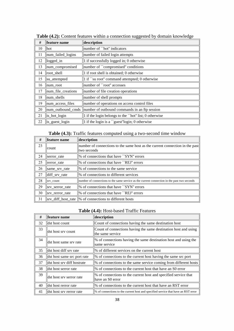
38
Table (4.2): Content features within a connection suggested by domain knowledge
# feature name description
11 hot number of ``hot'' indicators
11 num_failed_logins number of failed login attempts
12 logged_in 1 if successfully logged in; 0 otherwise
13 num_compromised number of ``compromised'' conditions
14 root_shell 1 if root shell is obtained; 0 otherwise
15 su_attempted 1 if ``su root'' command attempted; 0 otherwise
16 num_root number of ``root'' accesses
17 num_file_creations number of file creation operations
18 num_shells number of shell prompts
19 num_access_files number of operations on access control files
21 num_outbound_cmds number of outbound commands in an ftp session
21 is_hot_login 1 if the login belongs to the ``hot'' list; 0 otherwise
22 is_guest_login 1 if the login is a ``guest''login; 0 otherwise
Table (4.3): Traffic features computed using a two-second time window
# feature name description
23 count
number of connections to the same host as the current connection in the past
two seconds
24 serror_rate % of connections that have ``SYN'' errors
25 rerror_rate % of connections that have ``REJ'' errors
26 same_srv_rate % of connections to the same service
27 diff_srv_rate % of connections to different services
28 srv_count number of connections to the same service as the current connection in the past two seconds
29 srv_serror_rate % of connections that have ``SYN'' errors
31 srv_rerror_rate % of connections that have ``REJ'' errors
31 srv_diff_host_rate % of connections to different hosts
Table (4.4): Host-based Traffic Features
# feature name description
32 dst host count Count of connections having the same destination host
33 dst host srv count
Count of connections having the same destination host and using
the same service
34 dst host same srv rate
% of connections having the same destination host and using the
same service
35 dst host diff srv rate % of different services on the current host
36 dst host same src port rate % of connections to the current host having the same src port
37 dst host srv diff hostrate % of connections to the same service coming from different hosts
38 dst host serror rate % of connections to the current host that have an S0 error
39 dst host srv serror rate
% of connections to the current host and specified service that
have an S0 error
40 dst host rerror rate % of connections to the current host that have an RST error
41 dst host srv rerror rate % of connections to the current host and specified service that have an RST error

39
4.2.3 Data sets Sample: Sample of data sets was chosen randomly as shown in Table 4.5. Some
features were chosen because there is no space to show all features [53] [54].
Table (4.5): Sample of data sets
# type duration protocol type service flag src bytes dst bytes
1 normal. 0 tcp http SF 181 5450
2 normal. 0 tcp http SF 217 2032
3 smurf. 0 icmp ecr_i SF 1032 0
4 neptune. 0 tcp private S0 0 0
5 normal. 2 tcp smtp SF 1572 437
6 normal. 2 udp domain_u SF 93 37
The KDD dataset consists of three components: "Whole KDD", "Corrected KDD"
and "10% KDD" as illustrated in Table 4.6, Also 10% KDD types and counts Table
4.7 [54].
Table (4.6): KDD Cup 99 Datasets type and counts
KDD dataset Normal DoS Probe R2L U2R
Whole 972780 3883370 41102 1126 52
Corrected 60593 229853 4166 16347 70
10% 97277 391458 4107 1126 52
Table (4.7): KDD Cup 99 10% Datasets type and counts
4.2.4 Data sets Attacks Types:
The KDD dataset can be classified into four main categories of attacks:
Denial-of-service attack (DoS): is a class of attacks where an attacker makes some
computing or memory resource too busy or too full to respond to requests, ex. smurf,
neptune, back, teardrop, pod and land.
Probing (Probe): is a class of attacks where an attacker scans a network to get some
information about potential vulnerabilities in the network, ex. satan, ipsweep,
portsweep and nmap.
User to Root Attacks (R2L): is a class of attacks where an attacker gets an access to
a normal user account on the system to get a root user access to the system later, ex.
warezclient, guess_passwd, warezmaster, ftp_write, multihop, phf, spy and imap.
KDD
dataset
Normal Abnormal Total
DoS Probe R2L U2R
10% 97277 391458 4107 1126 52
∑ 97277 396743 494020
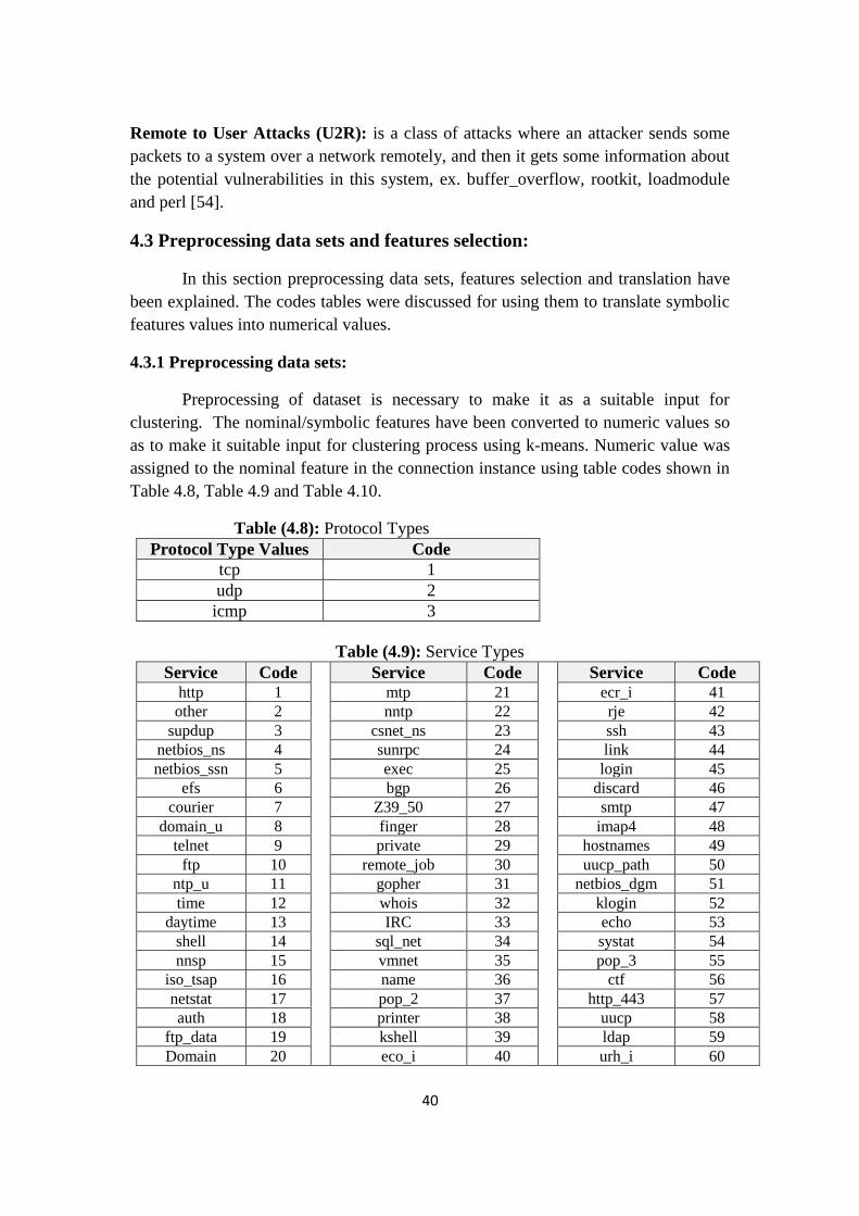
41
Remote to User Attacks (U2R): is a class of attacks where an attacker sends some
packets to a system over a network remotely, and then it gets some information about
the potential vulnerabilities in this system, ex. buffer_overflow, rootkit, loadmodule
and perl [54].
4.3 Preprocessing data sets and features selection:
In this section preprocessing data sets, features selection and translation have
been explained. The codes tables were discussed for using them to translate symbolic
features values into numerical values.
4.3.1 Preprocessing data sets:
Preprocessing of dataset is necessary to make it as a suitable input for
clustering. The nominal/symbolic features have been converted to numeric values so
as to make it suitable input for clustering process using k-means. Numeric value was
assigned to the nominal feature in the connection instance using table codes shown in
Table 4.8, Table 4.9 and Table 4.10.
Table (4.8): Protocol Types
Protocol Type Values Code
tcp 1
udp 2
icmp 3
Table (4.9): Service Types
Service Code Service Code Service Code http 1 mtp 21 ecr_i 41
other 2 nntp 22 rje 42
supdup 3 csnet_ns 23 ssh 43
netbios_ns 4 sunrpc 24 link 44
netbios_ssn 5 exec 25 login 45
efs 6 bgp 26 discard 46
courier 7 Z39_50 27 smtp 47
domain_u 8 finger 28 imap4 48
telnet 9 private 29 hostnames 49
ftp 10 remote_job 30 uucp_path 50
ntp_u 11 gopher 31 netbios_dgm 51
time 12 whois 32 klogin 52
daytime 13 IRC 33 echo 53
shell 14 sql_net 34 systat 54
nnsp 15 vmnet 35 pop_3 55
iso_tsap 16 name 36 ctf 56
netstat 17 pop_2 37 http_443 57
auth 18 printer 38 uucp 58
ftp_data 19 kshell 39 ldap 59
Domain 20 eco_i 40 urh_i 60
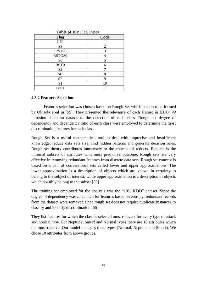
41
Table (4.10): Flag Types
Flag Code REJ 1
S3 2
RSTO 3
RSTOS0 4
S0 5
RSTR 6
S2 7
SH 8
SF 9
S1 10
OTH 11
4.3.2 Features Selection:
Features selection was chosen based on Rough Set which has been performed
by Olusola et-al in [55]. They presented the relevance of each feature in KDD ’99
intrusion detection dataset to the detection of each class. Rough set degree of
dependency and dependency ratio of each class were employed to determine the most
discriminating features for each class.
Rough Set is a useful mathematical tool to deal with imprecise and insufficient
knowledge, reduce data sets size, find hidden patterns and generate decision rules.
Rough set theory contributes immensely to the concept of reducts. Reducts is the
minimal subsets of attributes with most predictive outcome. Rough sets are very
effective in removing redundant features from discrete data sets. Rough set concept is
based on a pair of conventional sets called lower and upper approximations. The
lower approximation is a description of objects which are known in certainty to
belong to the subject of interest, while upper approximation is a description of objects
which possibly belong to the subset [55].
The training set employed for the analysis was the “10% KDD” dataset. Since the
degree of dependency was calculated for features based on entropy, redundant records
from the dataset were removed since rough set does not require duplicate instances to
classify and identify discrimination [55].
They list features for which the class is selected most relevant for every type of attack
and normal case. For Neptune, Smurf and Normal types there are 18 attributes which
the most relative. Our model manages three types (Normal, Neptune and Smurf). We
chose 18 attributes from above groups.
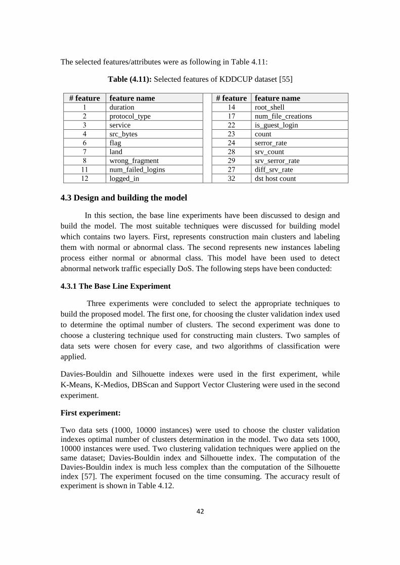
42
The selected features/attributes were as following in Table 4.11:
Table (4.11): Selected features of KDDCUP dataset [55]
# feature feature name # feature feature name 1 duration 14 root_shell
2 protocol_type 17 num_file_creations
3 service 22 is_guest_login
4 src_bytes 23 count
6 flag 24 serror_rate
7 land 28 srv_count
8 wrong_fragment 29 srv_serror_rate
11 num_failed_logins 27 diff_srv_rate
12 logged_in 32 dst host count
4.3 Design and building the model
In this section, the base line experiments have been discussed to design and
build the model. The most suitable techniques were discussed for building model
which contains two layers. First, represents construction main clusters and labeling
them with normal or abnormal class. The second represents new instances labeling
process either normal or abnormal class. This model have been used to detect
abnormal network traffic especially DoS. The following steps have been conducted:
4.3.1 The Base Line Experiment
Three experiments were concluded to select the appropriate techniques to
build the proposed model. The first one, for choosing the cluster validation index used
to determine the optimal number of clusters. The second experiment was done to
choose a clustering technique used for constructing main clusters. Two samples of
data sets were chosen for every case, and two algorithms of classification were
applied.
Davies-Bouldin and Silhouette indexes were used in the first experiment, while
K-Means, K-Medios, DBScan and Support Vector Clustering were used in the second
experiment.
First experiment:
Two data sets (1000, 10000 instances) were used to choose the cluster validation
indexes optimal number of clusters determination in the model. Two data sets 1000,
10000 instances were used. Two clustering validation techniques were applied on the
same dataset; Davies-Bouldin index and Silhouette index. The computation of the
Davies-Bouldin index is much less complex than the computation of the Silhouette
index [57]. The experiment focused on the time consuming. The accuracy result of
experiment is shown in Table 4.12.
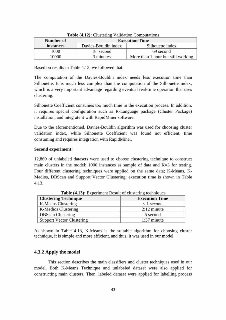
43
Table (4.12): Clustering Validation Computations
Number of
instances
Execution Time
Davies-Bouldin index Silhouette index
1000 18 second 69 second
10000 3 minutes More than 1 hour but still working
Based on results in Table 4.12, we followed that:
The computation of the Davies-Bouldin index needs less execution time than
Silhouette. It is much less complex than the computation of the Silhouette index,
which is a very important advantage regarding eventual real-time operation that uses
clustering.
Silhouette Coefficient consumes too much time in the execution process. In addition,
it requires special configuration such as R-Language package (Cluster Package)
installation, and integrate it with RapidMiner software.
Due to the aforementioned, Davies-Bouldin algorithm was used for choosing cluster
validation index, while Silhouette Coefficient was found not efficient, time
consuming and requires integration with RapidMiner.
Second experiment:
12,860 of unlabeled datasets were used to choose clustering technique to construct
main clusters in the model; 1000 instances as sample of data and K=3 for testing.
Four different clustering techniques were applied on the same data; K-Means, K-
Medios, DBScan and Support Vector Clustering; execution time is shown in Table
4.13.
Table (4.13): Experiment Result of clustering techniques
Clustering Technique Execution Time
K-Means Clustering < 1 second
K-Medios Clustering 2:12 minute
DBScan Clustering 5 second
Support Vector Clustering 1:37 minute
As shown in Table 4.13, K-Means is the suitable algorithm for choosing cluster
technique, it is simple and more efficient, and thus, it was used in our model.
4.3.2 Apply the model
This section describes the main classifiers and cluster techniques used in our
model. Both K-Means Technique and unlabeled dataset were also applied for
constructing main clusters. Then, labeled dataset were applied for labelling process
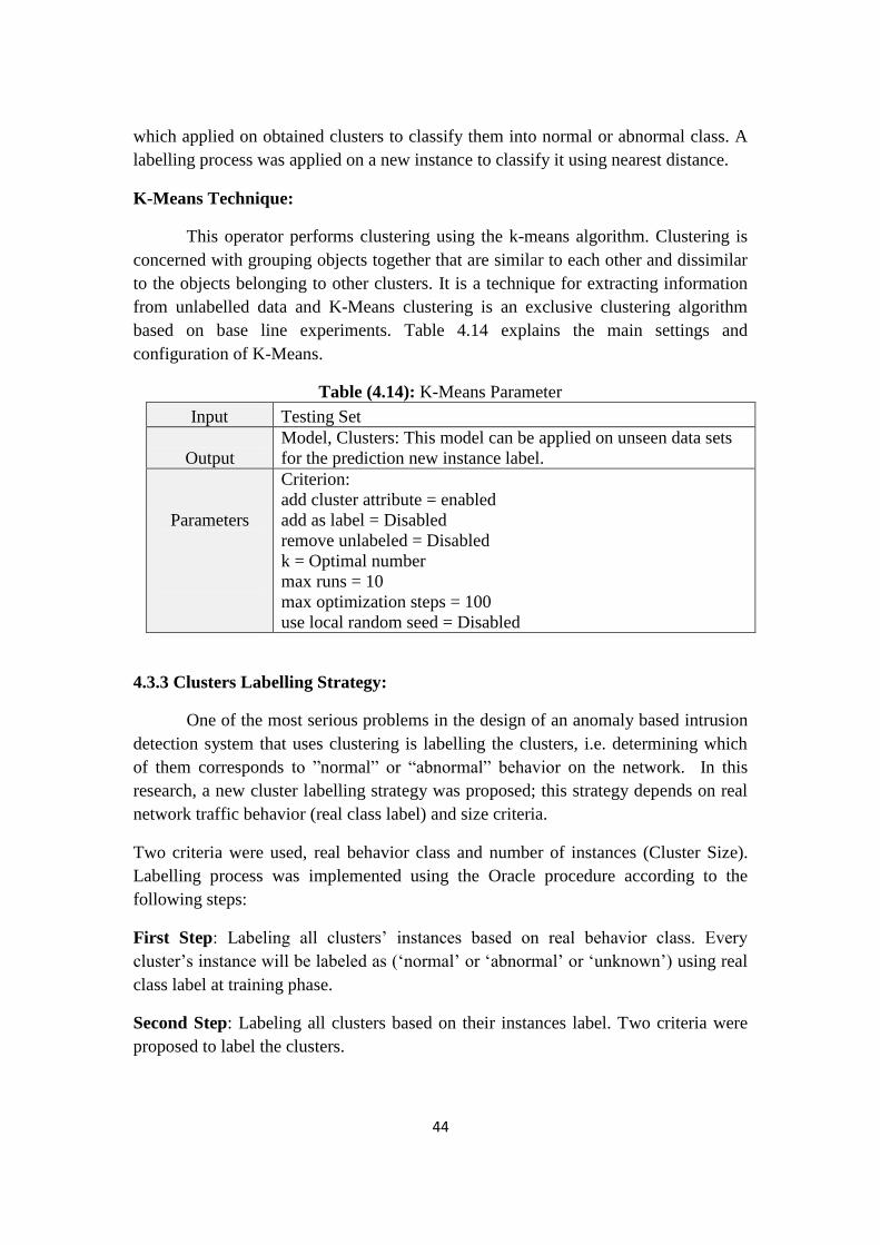
44
which applied on obtained clusters to classify them into normal or abnormal class. A
labelling process was applied on a new instance to classify it using nearest distance.
K-Means Technique:
This operator performs clustering using the k-means algorithm. Clustering is
concerned with grouping objects together that are similar to each other and dissimilar
to the objects belonging to other clusters. It is a technique for extracting information
from unlabelled data and K-Means clustering is an exclusive clustering algorithm
based on base line experiments. Table 4.14 explains the main settings and
configuration of K-Means.
Table (4.14): K-Means Parameter
Input Testing Set
Output
Model, Clusters: This model can be applied on unseen data sets
for the prediction new instance label.
Parameters
Criterion:
add cluster attribute = enabled
add as label = Disabled
remove unlabeled = Disabled
k = Optimal number
max runs = 10
max optimization steps = 100
use local random seed = Disabled
4.3.3 Clusters Labelling Strategy:
One of the most serious problems in the design of an anomaly based intrusion
detection system that uses clustering is labelling the clusters, i.e. determining which
of them corresponds to ”normal” or “abnormal” behavior on the network. In this
research, a new cluster labelling strategy was proposed; this strategy depends on real
network traffic behavior (real class label) and size criteria.
Two criteria were used, real behavior class and number of instances (Cluster Size).
Labelling process was implemented using the Oracle procedure according to the
following steps:
First Step: Labeling all clusters’ instances based on real behavior class. Every
cluster’s instance will be labeled as (‘normal’ or ‘abnormal’ or ‘unknown’) using real
class label at training phase.
Second Step: Labeling all clusters based on their instances label. Two criteria were
proposed to label the clusters.

45
After all instances are labeled:
If a cluster contains only normal labels then label it as ‘normal’.
If a cluster contains only abnormal labels then label it as ‘abnormal’.
If a cluster contains mixture of normal and abnormal instances, then we can
use one of two strategies:
The First Strategy: based on real behavior class and cluster size threshold:
If a cluster contains a mixture of normal and abnormal instances, then it needs to
be split into two clusters. The first one contains normal instance which have
greater size than our threshold size, while the second cluster contains the remained
instances that have abnormal behavior.
The Second Strategy: based on real behavior class only:
If a cluster contains a mixture of normal and abnormal instances, then it needs to
be split into two clusters, contain normal instances and abnormal instances,
respectively.
In this phase, unknown instances (neither normal nor abnormal) can be
manipulated and labeled after labeling all clusters.
4.3.4 New Instances Labeling Strategy:
For every new instance, Euclidean Distance was chosen as the metric to calculate the
distance among the instance and the labeled clusters. If the instance’s distance is near
to normal cluster then label it as ‘normal’ otherwise label it as ‘abnormal’. New
instances labelling process was implemented using the Oracle procedure.
4.4 Evaluation of the Model:
Performance evaluation of the model is one of the most important missions of
the research. The effectiveness of the model is evaluated by its capability to make
accurate predictions. According to the real nature of a given event compared to the
prediction from the model, four possible outcomes are shown in Table 4.18, known as
the Confusion Matrix [51].
Confusion Matrices were used to evaluate clusters labeling process. Columns and
rows of the matrix represent actual label and the instance of predicate label,
respectively.
The following four parameters define the member of matrix:
True positive (TP) is shown in (Eq. 4.1).

46
True negative (TN) is shown in (Eq. 4.2).
False positive (FP) is shown in (Eq. 4.3).
False negative (FN) is shown in (Eq. 4.4).
The accuracy of the model is considered to be the most commonly measurement to
evaluate the performance. Accuracy (Eq. 4.5), detection rate (Eq. 4.6) and false alarm
(Eq. 4.7) were used in this research for model evaluation
Confusion Matrix: was created after labeling clustering or labeling a new instance.
The main elements in the matrix are shown in Table 4.15:
Table (4.15): Confusion Matrix Structure
True positive (TP) refers to positive instances that correctly labeled the classifier
(When abnormal data detected as abnormal).
True Positive rate = TP / ( TP + FN ) (Eq. 4.1).
True negative (TN) refers to negative instances that correctly labeled the
classifier (when normal data detected as normal).
True Negative rate = TN / ( TN + FP ) (Eq. 4.2).
False Positive (FP) is the negative instances that were incorrectly labeled (when
normal data detected as abnormal)
False Positive rate = FP / ( FP + TN ) (Eq. 4.3).
False Negative (FN) is the positive instances that were incorrectly labeled (when
abnormal data detected as normal)
False Positive rate = FN / ( FN + TP ) (Eq. 4.4).
Actual (True) Class
Actual Normal
(Positive)
Actual Abnormal
(Negative)
Predicate
Class
Predicate Normal
(Positive)
True positive (TP) False positive (FP)
Predicate Abnormal
(Negative)
False negative (FN) True negative (TN)
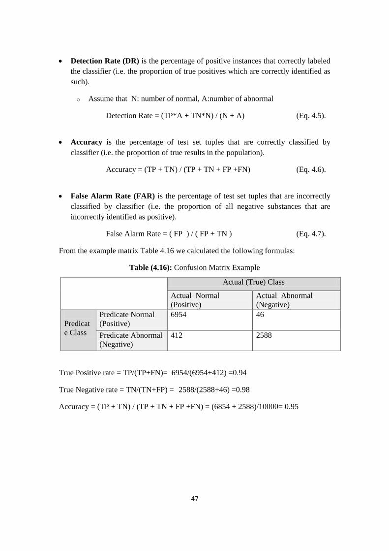
47
Detection Rate (DR) is the percentage of positive instances that correctly labeled
the classifier (i.e. the proportion of true positives which are correctly identified as
such).
o Assume that N: number of normal, A:number of abnormal
Detection Rate = (TP*A + TN*N) / (N + A) (Eq. 4.5).
Accuracy is the percentage of test set tuples that are correctly classified by
classifier (i.e. the proportion of true results in the population).
Accuracy = (TP + TN) / (TP + TN + FP +FN) (Eq. 4.6).
False Alarm Rate (FAR) is the percentage of test set tuples that are incorrectly
classified by classifier (i.e. the proportion of all negative substances that are
incorrectly identified as positive).
False Alarm Rate = ( FP ) / ( FP + TN ) (Eq. 4.7).
From the example matrix Table 4.16 we calculated the following formulas:
Table (4.16): Confusion Matrix Example
True Positive rate = TP/(TP+FN)= 6954/(6954+412) =0.94
True Negative rate = TN/(TN+FP) = 2588/(2588+46) =0.98
Accuracy = (TP + TN) / (TP + TN + FP +FN) = (6854 + 2588)/10000= 0.95
Actual (True) Class
Actual Normal
(Positive)
Actual Abnormal
(Negative)
Predicat
e Class
Predicate Normal
(Positive)
6954 46
Predicate Abnormal
(Negative)
412 2588

48
4.5 The proposed model:
The main objective of this research is to propose a new model for abnormal
network traffic detection especially DoS attack which is useful for intrusion detection
systems. This could be achieved by using multiple layers to construct the model. A
labeled data was used to label the main clusters in the model, then unlabeled data to
construct the clusters. Both real class and cluster size criteria were applied on the
clusters to label them. After that, for any new instance, we calculated the nearest
distance into clusters, labeled it with closed clusters’ label. Higher accuracy and better
detection could be achieved through this model. Also, we tried to overcome the
drawback of existing methods used in previous research.
The proposed model consists of nine steps shows in Figure 4.1, as follows:
Step1: Collecting network traffic data sets - especially DoS -, preprocessing them,
select some attributes more relative with other. Neptune and Smurf types of DoS were
chosen for our model. Data were segmented into two parts, the first part was used to
label the model clusters. The second part was used to build the model and construct
clusters of data. These clusters were classified into either normal or abnormal type.
Step2: Dividing the data into two training and testing data sets. The purpose of this
division of data was to use training dataset for clustering process in the model.
Testing dataset was used for labeling new instances.
Step3: Choosing the most relative attributes which were used in building the model.
These attributes have a high correlation with each other. The selection process was
done based on previous studies and scientific equations.
Step4: Normalizing dataset before the process of building model based on clustering,
testing dataset with specific attributes chosen in previous steps were used at this stage.
Pre-processing of dataset was necessary to make it as a suitable input for clustering
process.
Data set pre-processing was achieved by applying data transformation; symbolic
features were required to be transformed into numeric values in an attempt to make it
suitable input for clustering process. Codes tables were defined to assign numeric
value to the symbolic feature since the process of clustering (specially k-means) needs
numeric data only, the characters values were converted into numeric by giving
specific code for each type.
Step5: Choosing optimal number of clusters by using clustering validation or
clustering quality indexes. These indices were used to tell us how well the data were
grouped into clusters, i.e. to find the optimal number of clusters for clustering
algorithms.
49
There are several measurements for clustering qualities, such as Davies-Bouldin index
and Silhouette index. Clustering quality means clusters have good compactness
between instances within the same cluster and good separation between clusters.
Davies-Bouldin algorithm was applied on testing set to get number of clusters that
represents the optimal number of clusters.
Step6: Constructing Clusters by applying clustering technique on testing dataset after
preprocessing done. Clustering process was required to build main clusters that
represent main network traffic. Based on our experiments in (section 4. 3.1) K-means
algorithm was chosen as the best technique for clustering algorithm. The number of
clusters was required to be initialized and selected from the previous step.
This algorithm is sensitive to outliers; it also has the advantage of clear geometrical
and statistical meaning, but works conveniently with numerical attributes only. The
result clusters were labeled using labeling process.
Step7: Labeling clusters is a major challenge in abnormal detection. It means how we
can determine whether the cluster is normal or abnormal. More than one technique
were applied for labeling process. Real behavior class done from training phase was
used to check the instances behavior in every cluster. Every instance in the cluster
was labeled as normal, abnormal or unknown behavior.
If a cluster contains only normal labels then label it as ‘normal’. If it contains only
abnormal labels then label it as ‘abnormal’. If it contains normal and abnormal
instances, then we can use one of two strategies, as follows:
The first strategy based on real behavior class and cluster size threshold: If a cluster
contains a mixture of normal and abnormal instances, then it would be split into two
clusters. The first one contains normal instances with greater size than our threshold
size, while the second cluster contains remained instances with abnormal behavior.
The second strategy based on real behavior class only: If a cluster contains a mixture
of normal and abnormal instances, then it would be split into two clusters. The first
one contains normal instances, while the second contains abnormal instances.
Step8: Every a new traffic instance was labeled by using the nearest distance into the
labeled clusters. If near to the normal cluster then it will be label as normal, else label
it as abnormal. The Euclidean distance is chosen to calculate the distance among the
new instances and the model clusters. Since the Euclidean distance can deal only with
continuous types of data, all the symbolic features are transformation using codes
tables. There are two methods to calculate distance between new instance and labeled
clusters.

51
First method by calculating the distance between instance and every instance in the
clusters, then find the nearest distance. If the distance is within normal cluster then
label instance as normal else label instance as abnormal.
The second method relaying on calculating the clusters centers (centroid) then
calculate the distance between instance and the clusters centroid. After that, find the
nearest distance, if this distance within normal cluster then label instance as normal
else label instance as abnormal. This step will be repeated until all instances are
labeled.
Step9: The result from clusters labeling and labeling instances will be estimated. The
performance measurements were calculated by computing accuracy, detection rate
and false alarm. Confusion Matrices considered the most effective method to measure
the model efficiency and accuracy. It was used to evaluation measures clusters
labeling method, and labels a new instance. Each column of the matrix represent
actual label, while each row represents the instance of predicate label. We calculated
the member of matrix such as true positive, true negative, false positive and False
negative.

51
4.6 Summary:
In the following Table 4.17 the summary of the processes for the proposed model was
shown briefly.
Table (4.17): The proposed model processes
Step# Process Description
Step1 Collecting network traffic data sets - especially DoS -, preprocessing them, select
some attributes more relative with other. Neptune and Smurf types of DoS were
chosen for our model.
Step2 Dividing the data into two training and testing data sets.
Step3 Choosing the most relative attributes which were used in building the model.
These attributes have a high correlation with each other.
Step4 Normalizing dataset before the process of building model based on clustering,
testing dataset with specific attributes chosen in previous steps were used at this
stage.
Step5 Choosing optimal number of clusters by using clustering validation or clustering
quality indexes.
Step6 Constructing Clusters by applying clustering technique on testing dataset after
preprocessing done. Clustering process was required to build main clusters that
represent main network traffic.
Step7 Labeling clusters is a major challenge in abnormal detection. It means how we
can determine whether the cluster is normal or abnormal.
Step8 Every a new traffic instance was labeled using by the nearest distance into the
labeled clusters. If near to the normal cluster then it will label as normal, else
label it as abnormal.
Step9 The result from clusters labeling and labeling instances will be estimated. The
performance measurements were calculated by computing accuracy, detection
rate and false alarm.

52
Figure (4.3): The Proposed Model
Data Set (Raw Data)
Testing Dataset Training Dataset
New Traffic Instance
Normalize (Nominal to Numerical) K-means needs numeric Ex. “http”=1
fdsfsd
Select Optimal Number of Clusters (K)
Feature Selection
Clustering by (K-Means)
Label Clusters (Real Class, Size)
Calculation Distant from Cluster
Near to Normal Cluster
Yes No
End
Label as Normal Label as Abnormal
Accuracy
Split Cluster
Any Cluster has Multi Behavior
Yes
All Instances are labeled
Yes
No No

53
Chapter 5: Experimental Results and Evaluation
In this chapter, the experiments results were presented and analyzed. The
tools, requirements and environments used in our model were explained. After
labeling process for clusters and new instances, main evaluation measurements such
accuracy, detection rate and false alarm were calculated.
5.1 Experiments Setup:
This section describes the experiments environment and tools used to measure
the performance evaluation of clustering label of the proposed model.
5.1.1 Experimental Environments and Tools:
The experiments were conducted using an Intel® Core™2 Duo CPU 2.4GHz
with 2.0GB RAM. Special programs were used for constructing the model and
implementation of model functions, such as:
RapidMiner Program: RapidMiner [10] is an international open-source data mining
framework. It enables users to model complex knowledge discovery processes as it
supports nested operator chains. Graphical User Interface feature of RapidMiner
enables it to be used for complex process modeling. Moreover, it can be used as a
library in other programs.
RapidMiner is commonly used as a data mining tool for many reasons. First, it has
many data loading, modeling, preprocessing and visualization methods that avoid the
trouble of preprocessing data sets and help to visualize the results. It is easy to use the
currently robust graphical user interface that facilitates the modeling of different
complex processes. Second, it is modular and thus allows using some functionalities
for the extension, for example, using distance measurements for anomaly detection
operators. Finally, it is easily extensible and was used for clustering data and
construct network traffic behavior using K-Means algorithm and Decision Tree,
respectively.
Oracle Database10g (SQL+PL/SQL): Oracle Software [67] was used for clusters
labeling process and calculation minimum distance (Euclidian Distance). The main
evaluations measurements equations were implemented.
Microsoft Excel: It was used for dataset representation and storing results for clusters
labeling process.
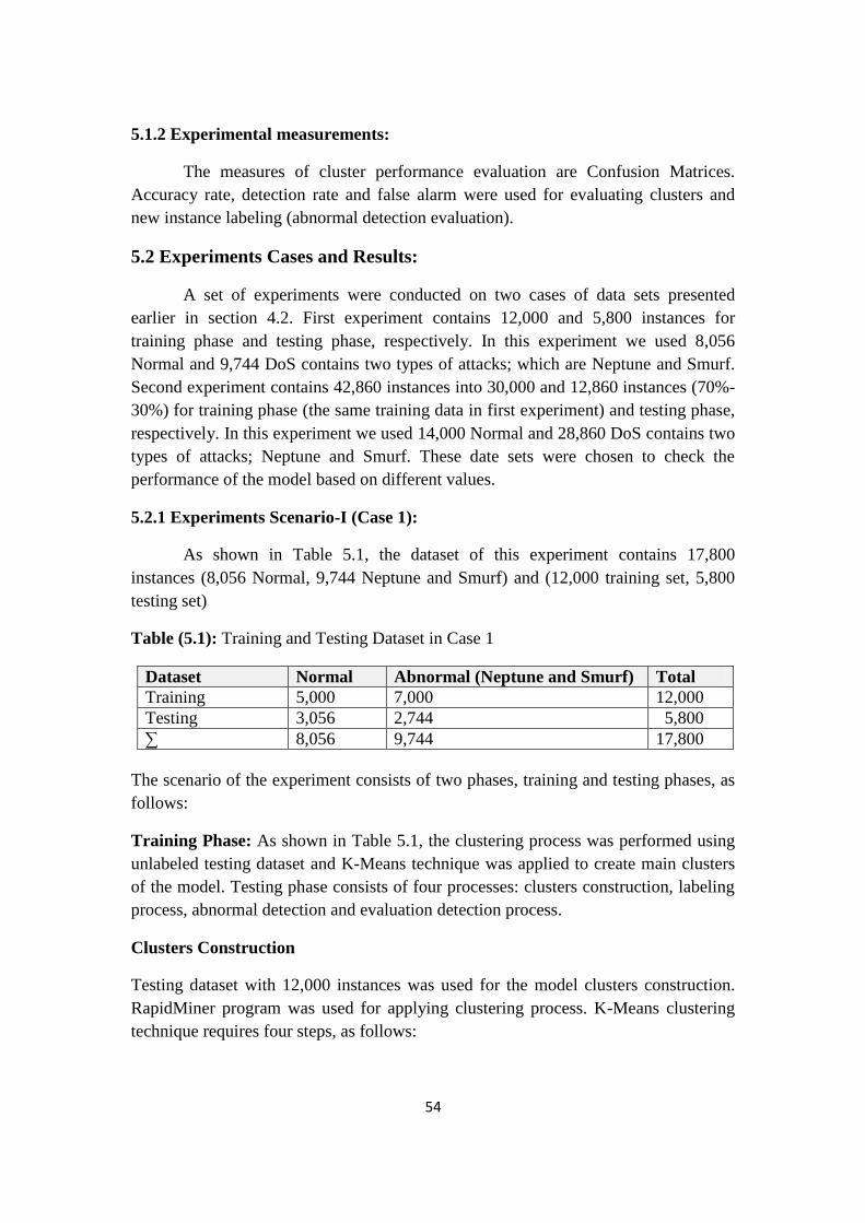
54
5.1.2 Experimental measurements:
The measures of cluster performance evaluation are Confusion Matrices.
Accuracy rate, detection rate and false alarm were used for evaluating clusters and
new instance labeling (abnormal detection evaluation).
5.2 Experiments Cases and Results:
A set of experiments were conducted on two cases of data sets presented
earlier in section 4.2. First experiment contains 12,000 and 5,800 instances for
training phase and testing phase, respectively. In this experiment we used 8,056
Normal and 9,744 DoS contains two types of attacks; which are Neptune and Smurf.
Second experiment contains 42,860 instances into 30,000 and 12,860 instances (70%-
30%) for training phase (the same training data in first experiment) and testing phase,
respectively. In this experiment we used 14,000 Normal and 28,860 DoS contains two
types of attacks; Neptune and Smurf. These date sets were chosen to check the
performance of the model based on different values.
5.2.1 Experiments Scenario-I (Case 1):
As shown in Table 5.1, the dataset of this experiment contains 17,800
instances (8,056 Normal, 9,744 Neptune and Smurf) and (12,000 training set, 5,800
testing set)
Table (5.1): Training and Testing Dataset in Case 1
Dataset Normal Abnormal (Neptune and Smurf) Total
Training 5,000 7,000 12,000
Testing 3,056 2,744 5,800
∑ 8,056 9,744 17,800
The scenario of the experiment consists of two phases, training and testing phases, as
follows:
Training Phase: As shown in Table 5.1, the clustering process was performed using
unlabeled testing dataset and K-Means technique was applied to create main clusters
of the model. Testing phase consists of four processes: clusters construction, labeling
process, abnormal detection and evaluation detection process.
Clusters Construction
Testing dataset with 12,000 instances was used for the model clusters construction.
RapidMiner program was used for applying clustering process. K-Means clustering
technique requires four steps, as follows:

55
Feature Selection: The most relevant features for the model were: duration,
protocol_type, service, flag, src_bytes, land, wrong_fragment, num_failed_logins,
logged_in, root_shell, num_file_creations, is_guest_login, count, srv_count,
serror_rate, srv_serror_rate, diff_srv_rate and dst_host_count [55].
Data Preprocessing and Transformation: All symbolic values were modified with
numerical ones as shown in Table 5.2.
Table (5.2): Features Translation Codes in Case 1
Features Name Code Value
Protocol Type 1..3
Service 1..60
Flag 1..11
Select Number of Clusters (K): Davies-Bouldin (DB) Index was applied on the
dataset using RapidMiner program. The minimum value of DB was chosen when
K=3, and it was the optimal number of clusters.
Clustering Data using (K-Means) with K=3: Clustering process was performed
using RapidMiner. K-Means technique was chosen for clustering with parameters
shown in Table 5.3. The clustering result is shown in both Table 5.4 and Figure 5.1.
Table (5.3): K-Means Parameters in Case 1
Input Testing Set
Output
Model Clusters (Labeled): This model can now be applied
on unlabeled data sets for the prediction new instance
label.
Parameters
add cluster attribute = enabled
add as label = Disabled
remove unlabeled = Disabled
k = 3
max runs = 10
max optimization steps = 100
use local random seed = Disabled
Table (5.4): Clustering Result using K-Means in Case 1
Cluster No Size
cluster_0 3629
cluster_1 3764
cluster_2 4607

56
Figure (5.1): Clustering Result using K-Means in Case 1
o Clusters Labelling Strategy:
Labeling clusters process consists of two steps implemented by the Oracle procedure,
as follows:
Clusters Labelling - First Step: Labeling all clusters’ instances based on real
behavior class. This process starts after clusters are constructed. Every cluster’s
instance labeled as normal or abnormal.
Results of labelling clusters’ instances are shown in both Table 5.5 and Figure 5.2.
Table (5.5): Labeled clusters’ instances result after first step
Cluster No Real Label # of instances PCT
cluster_0 Abnormal 3500 96.50%
cluster_0 Normal 129 3.50%
cluster_1 Abnormal 3500 92.99%
cluster_1 Normal 264 7.01%
cluster_2 Normal 4607 100%
Figure (5.2): Labeled clusters’ instances result after first step
Clusters Labelling - Second Step: Labeling all clusters based on their instances
label. This process starts after all instances were labeled. Two criteria were proposed
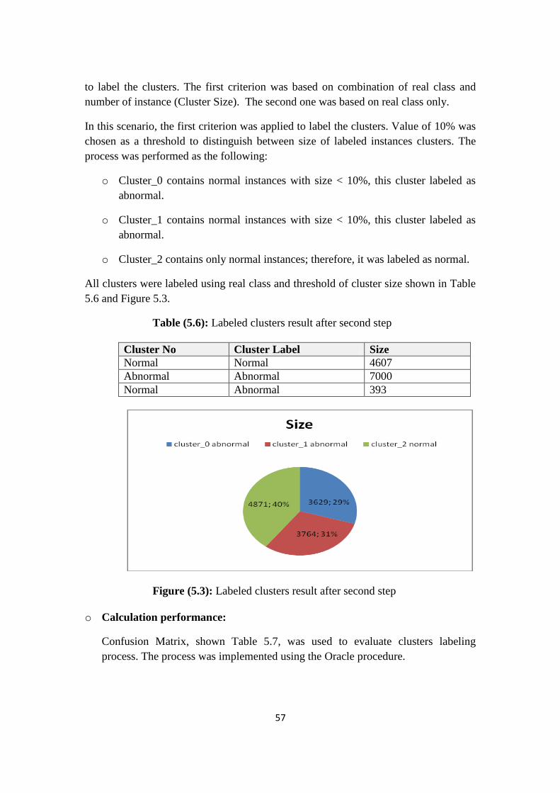
57
to label the clusters. The first criterion was based on combination of real class and
number of instance (Cluster Size). The second one was based on real class only.
In this scenario, the first criterion was applied to label the clusters. Value of 10% was
chosen as a threshold to distinguish between size of labeled instances clusters. The
process was performed as the following:
o Cluster_0 contains normal instances with size < 10%, this cluster labeled as
abnormal.
o Cluster_1 contains normal instances with size < 10%, this cluster labeled as
abnormal.
o Cluster_2 contains only normal instances; therefore, it was labeled as normal.
All clusters were labeled using real class and threshold of cluster size shown in Table
5.6 and Figure 5.3.
Table (5.6): Labeled clusters result after second step
Cluster No Cluster Label Size
Normal Normal 4607
Abnormal Abnormal 7000
Normal Abnormal 393
Figure (5.3): Labeled clusters result after second step
o Calculation performance:
Confusion Matrix, shown Table 5.7, was used to evaluate clusters labeling
process. The process was implemented using the Oracle procedure.

58
Table (5.7): Confusion Matrix for labeling clusters
Measurements Evaluation: Measurements evaluation of Accuracy, Detection Rate
and False Alarms were 96.07, 95.42 and zero, respectively.
The results shows that abnormal detection, especially DoS attack, using the
combination of both real network behavior class and cluster size threshold gives
satisfied results. The detection rate could be increased using different criteria for
labeling clusters, or by increasing the size of training dataset that represents the
behavior of network traffic.
5.2.2 Experiments Scenario-II (Case 2):
The dataset of this experiment of this case contains 18,660 instances. New
training dataset with 12,860 instances were used, while the same testing dataset with
5,800 were selected as shown in Table 5.8. In this scenario, two methods were applied
to label the clusters. First one was a combination of real behavior class and size, and
the second was real behavior class only. The results were more satisfied than scenario
I, and labeling process performance was checked and tested.
Table (5.8): Training and Testing Dataset in Case 2
Dataset Normal Abnormal (Neptune and Smurf) Total
Training 4,000 8,860 12,860
Testing 3,056 2,744 5,800
∑ 7,056 11,604 18,660
This scenario includes training and testing phases, as follows:
Training Phase: In this phase, clustering process was performed using unlabeled
testing dataset shown in Table 5.8, and K-Means clustering technique was applied to
create the main clusters of the model. Testing phase consists of four processes:
clusters construction, labeling process, abnormal detection and evaluation detection
process.
o Clusters Construction
As shown in Table 5.8, testing dataset with 12,860 instances were used for model
clusters construction. RapidMiner program was used for applying and performing
clustering process. Four steps were required for K-Means technique used in the
experiment, which are:
Actual Predicted Normal Predicted Abnormal
Normal 4607 393
Abnormal 0 7000

59
Feature Selection: The most relevant features for the model were: duration,
protocol_type, service, flag, src_bytes, land, wrong_fragment, num_failed_logins,
logged_in, root_shell, num_file_creations, is_guest_login, count, srv_count,
serror_rate, srv_serror_rate, diff_srv_rate and dst_host_count [55].
Data Preprocessing and Transformation: All symbolic values were modified with
numerical ones as shown in Table 5.9.
Table (5.9): Features Translation Codes in Case 2
Feature Name Code Value
Protocol Type 1..3
Service 1..60
Flag 1..11
Select Number of Clusters (K): Davies-Bouldin Index was applied on the dataset
using RapidMiner program. The results have minimum value of DB when K=3. It is
the optimal number of clusters.
Clustering Data using (K-Means) with K=3: Clustering process was performed
using RapidMiner. K-Means clustering technique was chosen with parameters shown
in Table 5.11. The clustering result is shown in both Table 5.10 and Figure 5.4.
Table (5.10): K-Means Parameters in Case 2
Input Testing Set
Output Clusters of Model
Parameters
add cluster attribute = enabled
add as label = Disabled
remove unlabeled = Disabled
k = 3
max runs = 10
max optimization steps = 100
use local random seed = Disabled
Table (5.11): Clustering Result using K-Means in Case 2
Cluster No Size
cluster_0 2
cluster_1 8195
cluster_2 4663

61
Figure (5.4): Clustering Result using K-Means in Case 2
o Clusters Labelling Strategy:
Labeling Clusters process consists of two steps; clustering labelling and clusters
labelling:
Clusters Labelling - First Step: Labeling all clusters’ instances was based on real
behavior class. This process started after clusters were constructed. Every cluster’s
instance was labeled as normal or abnormal.
The result of labelling clusters’ instances is shown in both Table 5.12 and Figure 5.5.
Table (5.12): Clusters’ Instances result after being labeled in Case 2 (First Step)
Cluster No Behavior Rules Label # of instances PCT
cluster_0 Normal 2 100
cluster_1 Abnormal 4360 93.5%
cluster_1 Normal 303 6.5%
cluster_2 Normal 3695 45.09%
cluster_2 Abnormal 4500 54.91%
Figure (5.5): Clusters’ Instances result after being labeled in Case 2 (First Step)
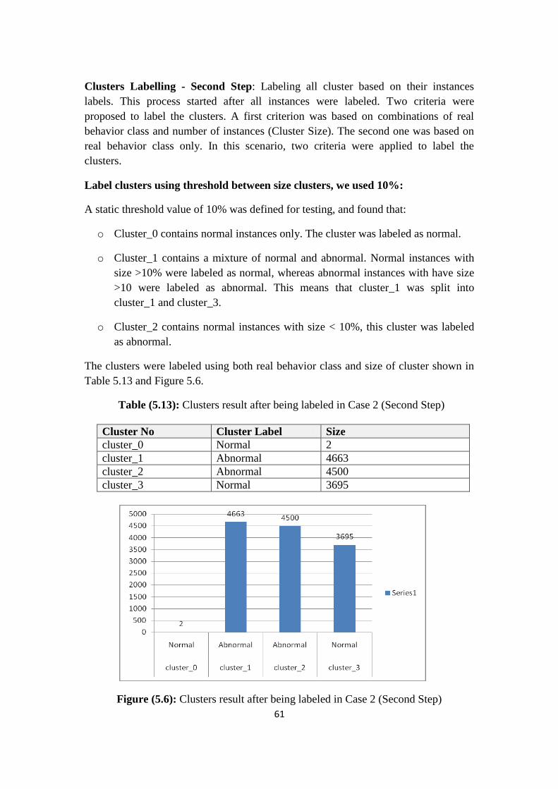
61
Clusters Labelling - Second Step: Labeling all cluster based on their instances
labels. This process started after all instances were labeled. Two criteria were
proposed to label the clusters. A first criterion was based on combinations of real
behavior class and number of instances (Cluster Size). The second one was based on
real behavior class only. In this scenario, two criteria were applied to label the
clusters.
Label clusters using threshold between size clusters, we used 10%:
A static threshold value of 10% was defined for testing, and found that:
o Cluster_0 contains normal instances only. The cluster was labeled as normal.
o Cluster_1 contains a mixture of normal and abnormal. Normal instances with
size >10% were labeled as normal, whereas abnormal instances with have size
>10 were labeled as abnormal. This means that cluster_1 was split into
cluster_1 and cluster_3.
o Cluster_2 contains normal instances with size < 10%, this cluster was labeled
as abnormal.
The clusters were labeled using both real behavior class and size of cluster shown in
Table 5.13 and Figure 5.6.
Table (5.13): Clusters result after being labeled in Case 2 (Second Step)
Cluster No Cluster Label Size
cluster_0 Normal 2
cluster_1 Abnormal 4663
cluster_2 Abnormal 4500
cluster_3 Normal 3695
Figure (5.6): Clusters result after being labeled in Case 2 (Second Step)

62
o Calculation performance:
As shown in Table 5.14, Confusion Matrix was used for clusters labeling method
evaluation.
Table (5.14): Confusion Matrices for clusters labeling in Case 2
Measurements Evaluation: Measurements evaluation of Accuracy, Detection Rate
and False Alarms were 96.21, 94.78 and 0, respectively.
But when value of 5% as threshold was applied:
All clusters have been labeled using real class and threshold of cluster size shown in
Table 5.15.
Table (5.15): Labeled clusters result after second step (5% threshold)
Cluster No Cluster Label Size
cluster_0 Normal 2
cluster_1 Abnormal 4360
cluster_1 Normal 303
cluster_2 Normal 3695
cluster_2 Abnormal 4500
Measurements Evaluation: Measurements evaluation of Accuracy, Detection Rate
and False Alarms were 100, 100 and zero, respectively.
Both high detection rate and low false alarm with a very good accuracy were achieved
the model is applied on DoS attack. Previous works assume that abnormal attack is
very small because it is very rare. They identify the biggest cluster as normal and the
smallest cluster is abnormal. High accuracy and satisfied detection rate could be
achieved in abnormal network traffic detection, especially DoS attack. The detection
rate could be increased up to 100% using either more labeling methods or decrease
the threshold value near to zero (real behavior class).
Label clusters using real behavior class:
Real behavior class was only used for labeling. All instances in the clusters
were labeled using real class, and then clusters were split according to their real class,
one as normal and another as abnormal.
Both Table 5.16 and Figure 5.7 present clustering results when instances were labeled
using real class:
Actual Predicted Normal Predicted Abnormal
Normal 3697 303
Abnormal 0 8860

63
Table (5.16): Clustering Result before labeled in Case2
Cluster No Real behavior class Size PCT
cluster_0 Normal 2 100%
cluster_1 Abnormal 4360 93.50%
cluster_1 Normal 303 6.5%
cluster_2 Normal 3695 45.09%
cluster_2 Abnormal 4500 54.91%
Figure (5.7): Clustering Result before labeled in Case2
Real behavior class process was applied for labeling clusters as follows:
Cluster_0 contains normal instances only, so labeled as normal.
Cluster_1 contains normal and abnormal, this cluster was split into two
clusters: normal and abnormal clusters.
cluster_1 => (cluster_3:normal , cluster_1:abnormal)
Cluster_2 contains normal and abnormal, this cluster was split into two
clusters: normal and abnormal clusters.
cluster_2 => (cluster_4: normal, cluster_2:abnormal)
We labeled the clusters using real behavior class of cluster shown in Table 5.17 and
Figure 5.8.
Table (5.17): Clustering Label Result based real behavior class in Case2
Cluster No Cluster Label (Behavior Rules) Size
cluster_0 Normal 2
cluster_1 Abnormal 4461
cluster_2 Abnormal 4360
cluster_3 Normal 3734
cluster_4 Normal 303

64
Figure (5.8): Clustering Label Result based real behavior class in Case2
Calculation performance:
We used Confusion Matrix shown Table 5.18 that used to evaluation measures
clusters labeling method.
Table (5.18): Confusion Matrix Result based real behavior class in Case2
Measurements Evaluation: Accuracy, Detection Rate and False Alarms were 100,
100 and zero, respectively.
Both high Detection Rate and low False Alarm could be achieved with a very good
Accuracy when applying labeling clusters based on behavior rules. Detection Rate
increased to 100% using real behavior class labeling methods which represented all
real class of dataset.
5.3 Clusters Labelling Discussion:
The clustering process was performed using K-Means algorithm. All cluster’s
instances were labeled using real behavior class. Two methods were adopted for
labeling the model's clusters:
First method (Figure 5.9): Specific threshold size value was identified (in our case
10%), if the normal labeled instances is less than threshold size, then the cluster is
labeled as abnormal and vice versa. the normal labeled instances is more than
threshold size, then the cluster is divided into two clusters according its behavior size,
one is normal and the second is abnormal.
Actual Predicted Normal Predicted Abnormal
Normal 4000 0
Abnormal 0 8860
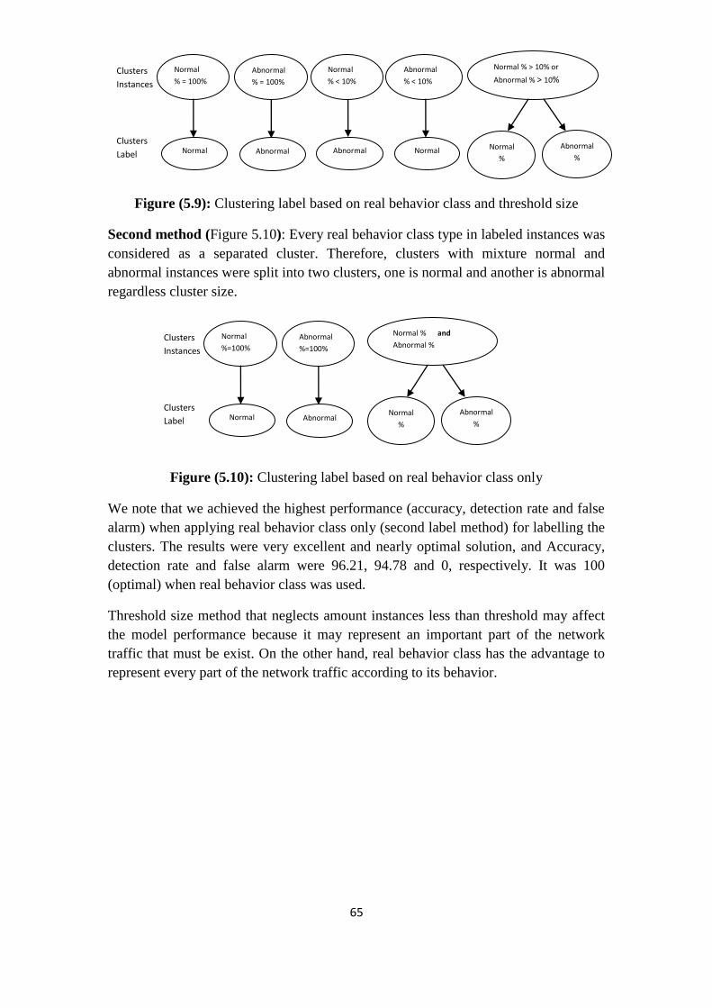
65
Figure (5.9): Clustering label based on real behavior class and threshold size
Second method (Figure 5.10): Every real behavior class type in labeled instances was
considered as a separated cluster. Therefore, clusters with mixture normal and
abnormal instances were split into two clusters, one is normal and another is abnormal
regardless cluster size.
Figure (5.10): Clustering label based on real behavior class only
We note that we achieved the highest performance (accuracy, detection rate and false
alarm) when applying real behavior class only (second label method) for labelling the
clusters. The results were very excellent and nearly optimal solution, and Accuracy,
detection rate and false alarm were 96.21, 94.78 and 0, respectively. It was 100
(optimal) when real behavior class was used.
Threshold size method that neglects amount instances less than threshold may affect
the model performance because it may represent an important part of the network
traffic that must be exist. On the other hand, real behavior class has the advantage to
represent every part of the network traffic according to its behavior.
Abnormal
Abnormal
% < 10%
Normal
Normal % > 10% or
Abnormal % > 10%
Abnormal
%
Normal
%
Normal
% < 10%
Abnormal
% = 100%
Abnormal
Normal
% = 100%
Normal
Clusters
Instances
Clusters
Label
Normal % and
Abnormal %
Abnormal
%
Normal
%
Abnormal
%=100%
Abnormal
Normal
%=100%
Normal
Clusters
Instances
Clusters
Label

66
Testing Phase: In this phase, new instances labeling technique was applied to label
new instances and check operation performance. Testing phase consists of labeling
new instance process.
5.4 Labeling New Instance:
In this section, testing data sets (10, 200 and 5800 instances) were randomly
chosen to test labeling a new instance after labeling the model clusters. For every new
instance, the nearest cluster into new instance was calculated using Euclidean
Distance equation [10] [38] [68]. If a new instance is near to normal cluster, then label
it as normal otherwise label it as abnormal (near to abnormal cluster). Both the
process and Euclidean Distance equation were implemented using the Oracle
procedure, if attribute is a symbolic then we assume all values have the same weight.
The following two methods were used to label a new instance:
The First method based on calculating the minimum distance between a new
instance and every instance in every cluster. If minimum distance was within normal
cluster instance, then label it as normal otherwise label it as abnormal.
The Second method based on calculating the clusters centroids as well as the
minimum distance between a new instance and every cluster’s centroid. If minimum
distance was within normal cluster centroid then label it as normal otherwise label it
as abnormal.
5.4.1 Labeling new instance - First Method: Find distance between all clusters’
instances and new instance using Euclidean Distance Equation.
Case 1: Using labeled clusters which are based on “Threshold size value”.
Scenario II (Case 2): Clusters were used in this experiment. 10 and 200 instances we
chosen for testing. The distance between the new instance and every instance in the
clusters which was labeled based on “Threshold size value” was calculated.
Small data sets were used for testing because calculation was waste time consuming.
Labeled clusters with 12860 instances were selected for time consuming estimation.
Calculation time is shown in Table 5.19.
Table (5.19): Euclidean Distance calculation time for labeling new instance
# Instance # Calculations Time (second)
1 12,860 4
10 12,8600 40
200 2,572,000 800 (13 min)
5000 64,300,000 5.55 Hours
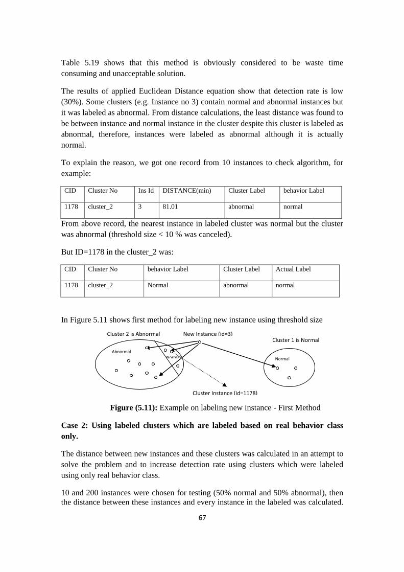
67
Table 5.19 shows that this method is obviously considered to be waste time
consuming and unacceptable solution.
The results of applied Euclidean Distance equation show that detection rate is low
(30%). Some clusters (e.g. Instance no 3) contain normal and abnormal instances but
it was labeled as abnormal. From distance calculations, the least distance was found to
be between instance and normal instance in the cluster despite this cluster is labeled as
abnormal, therefore, instances were labeled as abnormal although it is actually
normal.
To explain the reason, we got one record from 10 instances to check algorithm, for
example:
CID Cluster No Ins Id DISTANCE(min) Cluster Label behavior Label
1178 cluster_2 3 81.01 abnormal normal
From above record, the nearest instance in labeled cluster was normal but the cluster
was abnormal (threshold size < 10 % was canceled).
But ID=1178 in the cluster_2 was:
CID Cluster No behavior Label Cluster Label Actual Label
1178 cluster_2 Normal abnormal normal
In Figure 5.11 shows first method for labeling new instance using threshold size
Figure (5.11): Example on labeling new instance - First Method
Case 2: Using labeled clusters which are labeled based on real behavior class
only.
The distance between new instances and these clusters was calculated in an attempt to
solve the problem and to increase detection rate using clusters which were labeled
using only real behavior class.
10 and 200 instances were chosen for testing (50% normal and 50% abnormal), then
the distance between these instances and every instance in the labeled was calculated.
Normal
Abnormal
Cluster 2 is Abnormal
New Instance (id=3)
Normal
Cluster 1 is Normal
Cluster Instance (id=1178)

68
The result of detection rate after applied Euclidean Distance equation was 100%. This
is rarely happened. The result of applied Euclidean Distance equation for labeling all
instances was correct and detection rate was 100%. We believe that when instance
near into any labeled cluster, this cluster has only one type of behavior (normal or
abnormal). Figure 5.12 shows the first method for labeling new instance using real
behavior class only.
Figure (5.12): Example on labeling new instance using labeled clusters - Case2
5.4.2 Labeling new instance - Second Method: Find distance between clusters
centroid and new instances using Euclidean Distance Equation.
Case 1: Using Labeled clusters which labeled based on “Threshold size value”.
Labeled clusters which are labeled based on real behavior class and threshold size
were used. First, clusters centriod defined by: the centroid’s coordinate in the ith
dimension is the SUMi/N was calculated, SUMi/N is the sum in that dimension
divided by the number of points [8].
5800 instances were identified for testing and every cluster centroid as well as
calculated the distance between the instances and these centroids were calculated. The
result of applied Euclidean Distance equation is shown in both Table 5.20 and Figure
5.13:
Table (5.20): Label instances using distance and centroid of clusters Case 1
Cluster Label Instance Label Count
Abnormal Abnormal 2740
Normal Abnormal 118
Normal Unknown 27
Normal Normal 2911
Abnormal
Cluster 2 is Abnormal
New Instance
Normal
Cluster 1 is Normal
Normal
Cluster 3 is Normal
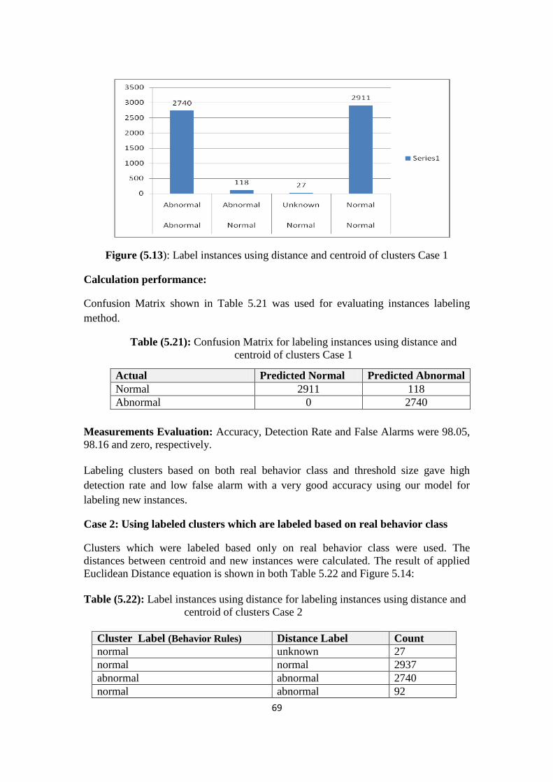
69
Figure (5.13): Label instances using distance and centroid of clusters Case 1
Calculation performance:
Confusion Matrix shown in Table 5.21 was used for evaluating instances labeling
method.
Table (5.21): Confusion Matrix for labeling instances using distance and
centroid of clusters Case 1
Measurements Evaluation: Accuracy, Detection Rate and False Alarms were 98.05,
98.16 and zero, respectively.
Labeling clusters based on both real behavior class and threshold size gave high
detection rate and low false alarm with a very good accuracy using our model for
labeling new instances.
Case 2: Using labeled clusters which are labeled based on real behavior class
Clusters which were labeled based only on real behavior class were used. The
distances between centroid and new instances were calculated. The result of applied
Euclidean Distance equation is shown in both Table 5.22 and Figure 5.14:
Table (5.22): Label instances using distance for labeling instances using distance and
centroid of clusters Case 2
Cluster Label (Behavior Rules) Distance Label Count
normal unknown 27
normal normal 2937
abnormal abnormal 2740
normal abnormal 92
Actual Predicted Normal Predicted Abnormal
Normal 2911 118
Abnormal 0 2740

71
Figure (5.14): Label instances using distance and centriod of clusters Case 2
Calculation performance:
As shown in Table 5.23, confusion matrix was used to evaluation measures
instances labeling method.
Table (5.23): Confusion Matrix for labeling instances using distance and
centroid of clusters Case 2
Measurements Evaluation: Accuracy, Detection Rate and False Alarms were 98.48,
98.56 and zero, respectively.
Labeling clusters based on real behavior class gave high detection rate and low false
alarm with very good accuracy and less performance than Case 1 using our model for
labeling new instances.
New Instances Labelling Discussion:
From our experiments, two methods were used to label a new instance. The first
method was based on minimum distance calculation between new instances and every
clusters instance. The second method was based on clusters centroids calculation, then
minimum distance calculation between new instances and every cluster’s centroid. If
the minimum distance within normal cluster, we labeled it as normal otherwise
abnormal. It was noticed that Euclidean Distance with clusters centroid could
achieved the highest performance (accuracy, detection rate and false alarm) as done in
second label method. The result was very excellent and near optimal values. The
Accuracy, Detection Rate and False Alarm were 98.48, 98.56 and zero, respectively.
Actual Predicted Normal Predicted Abnormal
Normal 2937 92
Abnormal 0 2740

71
5.3 Summary:
This section summarizes all experiments as follows:
Both Table 5.24 and Figure 5.15 show the summary of all clusters labelling
experiments' results that consists of main measurements of our model. Both Case2
and Case3 were chosen for representation as both Case1 and Case2 use the same
labeling criteria.
Table (5.24): Clusters Labelling Evaluation Measurements
Figure (5.15): Clusters Labelling Evaluation Measurements for Cases 2, 3
As shown in Table 5.25, both accepted accuracy and detection rate could be achieved
when using real behavior class only for labelling process. The false alarm was the
same in both methods. Therefore, the proposed model could achieve optimal result
when using real behavior class technique for labeling clusters process.
The following Table 5.25 and Figure 5.16 show the summary of labelling a new
instance according to Euclidean Distance equation. Both case 3 and case4 were
chosen for representation as Case1 and Case2 needed enough time which was
considered to be waste time and inapplicable technique.
Case
#
Labeling Criteria Training
Dataset
Accuracy
%
Detection
Rate
%
False
Alarm
% 1 real behavior class +
Threshold Size
12,000 96.07 95.42 0
2 real behavior class +
Threshold Size
12,860 96.21 94.78 0
3 real behavior class
12,860 100 100 0

72
Table (5.25): Instances Labelling Evaluation Measurements
Figure (5.16): Instances Labelling Evaluation Measurements
Table 5.26 shows that accepted accuracy and detection rate could be achieved with
the same false alarm for instances label using combination of clusters centroid, real
behavior class and threshold size.
Also, we calculated the difference between accuracy and detection rate of (clusters
centroid, real behavior class and threshold size) and (clusters centroid and real
behavior class); the difference was found very small. Accuracy difference :( 98.48-
98.05= 0.43%) , Detection rate difference: (98.56 - 98.16= 0.40%), so this means that
the proposed model could achieve good results using a combination of real behavior
class and threshold size method or only real behavior class method with clusters
centriod for labeling a new instance.
Case
#
Distance Criteria Test
instances
Accuracy
%
Detection
Rate
%
False
Alarm
% 1 Clusters instances , real behavior
class and threshold Size
10 30 0 70
2 Clusters instances , real behavior
class and threshold Size
200 100 100.0 0
3 Clusters centroid , real behavior
class and threshold Size
5800 98.05 98.16 0
4 Clusters centroid and real
behavior class
5800 98.48 98.56 0

73
Chapter 6: Conclusion and Future work
This chapter concludes the work, its results and discussion. The future work
directions were remarked.
6.1 Discussion and Summary:
Today, abnormal network traffic especially DoS is a critical threat on
computer network. There are several researches have been proposed to manipulate
this problem. The detection process based on intrusion detection system which
classified into network intrusion detection system and host based intrusion detection.
In this research, we proposed an efficient model using data mining techniques based
on Clustering technique. The clustering labeling technique was improved to able to
detect and classify types of abnormal network traffic such as DoS attack depend on
behavior anomaly detection approach, to achieve a higher accuracy and detection rate
with low false alarm rate.
The model consists of three phases:
Phase 1: In this phase, KDD Cup ‘99 dataset [53] was used, the most relevant
features for the model were selected.
Phase 2: In this phase, RapidMiner program was used to build the model clusters
using K-Means technique. Both the dataset and attributes from phase1 were used. The
symbolic attributes were replaced with numeric values. The optimal number of
clusters was determined using Davies-Bouldin index. After that, the instances of the
clusters were labeled using real behavior class. If a cluster contains instances with
only normal/abnormal behavior, then label it as their behavior. If a cluster contains
instances which have a mixture of behavior (normal and abnormal), the main cluster
was split into two clusters (one is normal and another is abnormal). Labelling process
is implemented by also Oracle procedure.
Phase 3: In this phase, Oracle procedure was used to label new instances according to
labeled clusters. The Euclidean distance is chosen as the metric to calculate the
distance among instances and centroid clusters. Every instance was labeled by
calculating the nearest distance from clusters. After that, the nearest distance was
calculated, if the distance within normal cluster (near to normal cluster) then label the
instance as normal otherwise label instance as abnormal.
Finally, the results showed that the proposed model has achieved a higher accuracy
and detection rate with low false alarm for labeling clusters process. The Accuracy,
Detection Rate and False Alarm were 96.21, 94.78 and zero respectively for using
both real class and threshold size, while the Accuracy and Detection Rate were 100
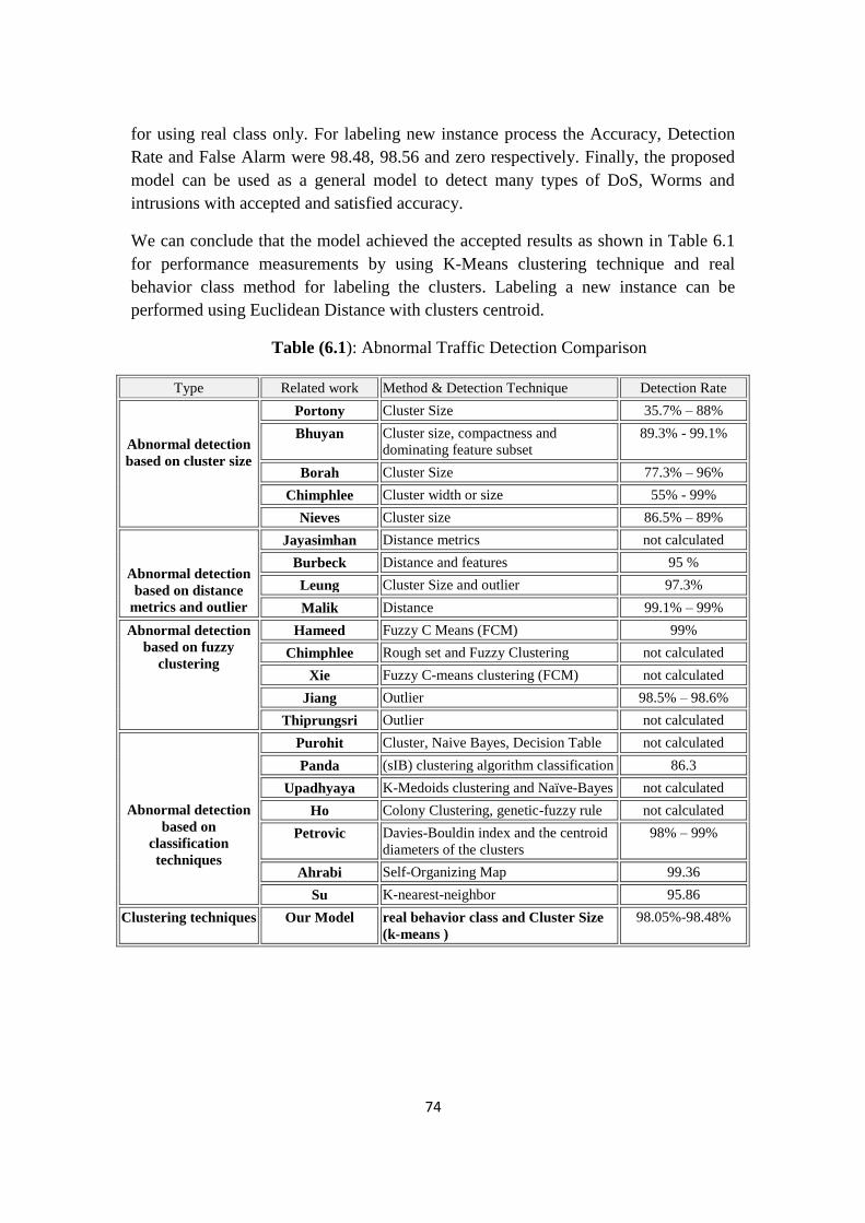
74
for using real class only. For labeling new instance process the Accuracy, Detection
Rate and False Alarm were 98.48, 98.56 and zero respectively. Finally, the proposed
model can be used as a general model to detect many types of DoS, Worms and
intrusions with accepted and satisfied accuracy.
We can conclude that the model achieved the accepted results as shown in Table 6.1
for performance measurements by using K-Means clustering technique and real
behavior class method for labeling the clusters. Labeling a new instance can be
performed using Euclidean Distance with clusters centroid.
Table (6.1): Abnormal Traffic Detection Comparison
Type Related work Method & Detection Technique Detection Rate
Abnormal detection
based on cluster size
Portony Cluster Size 35.7% – 88%
Bhuyan
Cluster size, compactness and
dominating feature subset
89.3% - 99.1%
Borah Cluster Size 77.3% – 96%
Chimphlee Cluster width or size 55% - 99%
Nieves Cluster size 86.5% – 89%
Abnormal detection
based on distance
metrics and outlier
Jayasimhan Distance metrics not calculated
Burbeck Distance and features 95 %
Leung Cluster Size and outlier 97.3%
Malik Distance 99.1% – 99%
Abnormal detection
based on fuzzy
clustering
Hameed Fuzzy C Means (FCM) 99%
Chimphlee Rough set and Fuzzy Clustering not calculated
Xie Fuzzy C-means clustering (FCM) not calculated
Jiang Outlier 98.5% – 98.6%
Thiprungsri Outlier not calculated
Abnormal detection
based on
classification
techniques
Purohit Cluster, Naive Bayes, Decision Table not calculated
Panda (sIB) clustering algorithm classification 86.3
Upadhyaya K-Medoids clustering and Naïve-Bayes not calculated
Ho Colony Clustering, genetic-fuzzy rule not calculated
Petrovic
Davies-Bouldin index and the centroid
diameters of the clusters
98% – 99%
Ahrabi Self-Organizing Map 99.36
Su K-nearest-neighbor 95.86
Clustering techniques
Our Model
real behavior class and Cluster Size
(k-means )
98.05%-98.48%

75
6.1 Future Work:
This study mainly focused on anomaly detection in large network based clustering
using DoS dataset. We used two types of DoS. There were other types such as
back, teardrop, pod and land which can be used in future work.
The Model can be applied on new types of abnormal such as Probing, User to
Root and Remote to User Attacks.
The Model can be applied on many types of worms or intrusions.
There are several clustering quality indexes that may be interesting to study for
choosing optimal number of clusters such as Dun index and c-index which can be
used in future work.
All ‘unknown’ instances which labeled them based on distance equation.
All new instances can be added into base clusters to increase labeling process
accuracy in the future.
The model can be a general model which can be used for detecting many types of
threats, DoS and Worms with accepted and satisfied accuracy.
76
References
[1] K. Leung and C. Leckie, Unsupervised Anomaly Detection In Network Intrusion
Detection Using Clusters, 2005.
[2] V. Gupta, S. khullar and M. kaur, Unsupervised Anomaly Detection in Network
Intrusion Detection Using Clusters.
[3] Wei Lu and I. Traore, Unsupervised anomaly detection using an evolutionary extension
of k-means algorithm, Int. J. Information and Computer Security 08/2001;
[4] RapidMiner, http://rapid-i.com/component/option,com_frontpage/Itemid,1/lang,en/
[Online] [Cited: May 10, 2013].
[5] J. Han and Micheline, Data Mining: Concepts and Techniques, Second Edition, 2006.
[6] V. Chandola and others, Anomaly Detection: A Survey, 2007.
[7] F. Silveira, C. Diot, N. Taft, R. Govindan, ASTUTE: detecting a different class of traffic
anomalies, Proceedings of the ACM SIGCOMM 2010 conference, August 30-September 03,
2010, New Delhi, India.
[8] Myung-Sup Kim, Hun-Jeong Kang, Seong-Cheol Hong, Seung-Hwa Chung, and James
W. Hong, A Flow-based Method for Abnormal Network Traffic Detection, 2004.
[9] http://en.wikipedia.org/wiki/Intrusion_detection_system. [Online] [Cited: March 20,
2013].
[10] C. Loo, M.Ng, C. Leckie and M. Palaniswami, Intrusion Detection for Routing Attacks
in Sensor Networks, 2006.
[11] T. Chen, Intrusion Detection for Viruses and Worms, 2004.
[12] http://en.wikipedia.org/wiki/Machine_learning. [Online] [Cited: March 20, 2013].
[13] S. Cherednichenko, Outlier Detection in Clustering, 2005.
[14] E. Paquet, “Exploring anthropometric data through cluster analysis”. Published in Digital
Human Modeling for Design and Engineering (DHM), pages, Rochester, MI, June, 2004.
[15] L. Kaufman and P. Rousseeuw, “Finding Groups in Data: An Introduction to Cluster
Analysis”. John Wiley Sons, New York, USA, 1990.
[16] J. Han and M. Kamber, “Data Mining: Concepts and Techniques”. The Morgan
Kaufmann Series in Data Management Systems, Jim Gray, Series Editor Morgan Kaufmann
Publishers, 550 pages, August 2000. (http://www.cs.sfu.ca/~han/DM_Book.html), visited
11.11.2004.
[17] B. Everitt , S. Landau , M. Leese ,D. Stahl, “Cluster analysis”. Publication
Date: February 21, 2011 | ISBN-10: 0470749911 | ISBN-13: 978-0470749913 |
Edition: 5
77
[18] S. Giha, R. Rasstogi and K. Shim, “CURE: an efficient clustering algorithm for
largedatabases”. In Proceedings of the 1998 ACM SIGMOD International Conference on
Management of Data, pages 73 – 84, June 1998.
[19] M. Ester, H-P. Kriegel, J. Sander and X. Xu, “A Density-based Algorithm for
Discovering Clusters in Large Spatial Databases with Noise”. In Proceedings of the Second
International Conference on Knowledge Discovery and Data Mining, pages 226 – 231, 1996.
[20] http://en.wikipedia.org/wiki/Data_mining. [Online] [Cited: March 20, 2013].
[21] X. Xu, M. Ester, H.-P. Kriegel, J. Sander, “A Distribution-based Clustering Algorithm
for Mining in Large Spatial Databases”. In Proceedings of the 14th International Conference
on Data Engineering, pages 324 – 331, February 1998.
[22] W. Wang, J. Yang and R. Muntz, “Sting: a Statistical Information Grid Approach to
Spatial Data Mining”. In Proceedings of the 23rd International Conference on Very Large
Data Bases (VLDB), pages 186 – 195, 1997.
[23] R. Agrawal, J. Gehrke, D. Gunopulos and P. Raghavan, “Automatic Subspace Clustering
of High Dimensional Data for Data Mining Applications”. In Proceedings of the ACM
SIGMOD International Conference on Management of Data, Volume 27, Issue 2, pages 94 –
105, June 1998.
[24] M. Sato, Y. Sato and L.C. Jain, “General Fuzzy Clustering Model and Neural Networks”.
In Proceedings of the Electronic Technology Directions to the Year 2000, pages 104 – 112,
May 1995.
[25] H. Jin, M.-L. Wong and K.-S. Leung, “Scalable Model-based Clustering by Working on
Data Summaries”. In Proceedings of the Third IEEE International Conference on Data
Mining, pages 91 – 98, November 2003.
[26] A. Tung, J. Hou and J. Han, “Spatial Clustering in the Presence of Obstacles”. In
Proceedings of the 17th International Conference on Data Engineering, pages 359 – 367,
April 2001.
[27] M. Halkidi, Y. Batiskakis and M. Vazirgiannis, “Clustering algorithm and validity
measures”. In Proceedings of the Thirteenth International Conference on Scientific and
Statistical Database Management, pages 3 – 22, Fairfax, Virginia, USA, July, 2001.
[28] C. Aggarwal and P. Yu, “Redefining Clustering for High-Dimensional Applications”. In
Proceedings of the IEEE International Conference on Transaction of Knowledge and Data
Engineering, Volume 14, Issue 2, pages 210 – 225, April 2002.
[29] I. Rao, Data Mining and Clustering Techniques, DRTC Workshop on Semantic Web 8th
– 10th December, 2003 DRTC, Bangalore.
[30] P. Grabusts The Choice Of Metrics For Clustering Algorithms, ISSN 1691-5402 ISBN
978-9984-44-071-2 Environment. Technology. Resources Proceedings of the 8th
International Scientific and Practical Conference. Volume I1 © Rēzeknes Augstskola,
Rēzekne, RA Izdevniecība, 2011.
78
[31]M. Halkidi, Y. Batistakis and M. Vazirgiannis, “Cluster Validity Methods: part I”. In
Proceedings of the ACM SIGMOD International Conference on Management of Data,
Volume 31, Issue 2, pages 40 – 45, June 2002.
[32] M. Halkidi, Y. Batistakis and M. Vazirgiannis, “Clustering Validity Checking Methods:
Part II”. In Proceedings of the ACM SIGMOD International Conference on Management of
Data, Volume 31, Issue 3, pages19 – 27, September 2002.
[33] Jose F. Nieves, Data Clustering for Anomaly Detection in Network Intrusion Detection,
2009.
[34] R. Storløkken, Labelling clusters in an anomaly based IDS by means of clustering
quality indexes, 2007.
[35] N. Bolshakova and F. Azuaje. Cluster validation techniques for genome expression data,
2003.
[36] S. Gunter and H. Bunke. Validation indices for graph clustering. Pattern Recogn. Lett.,
24(8):1107–1113, 2003.
[37] Liu, H., “Introduction to Data Mining”,2005.
[38] Han J. and Kamber M., Data Mining Concepts and Techniques, second edition,2006.
[39] Ye N., THE HANDBOOK OF DATA MINING, 2003.
[40] Portony L., Eskin E., Stolfo J. “Intrusion Detection with Unlabeled Data Using
Clustering”, Proceedings of ACM CSS Workshop on Data Mining Applied to Security
(DMSA-2001). Philadelphia, PA: November 5-8, 2001.
[41] A. purohit and H. Gupta, Hybrid Intrusion Detection System Model using Clustering,
Classification and Decision Table. IOSR Journal of Computer Engineering (IOSR-JCE) e-
ISSN: 2278-0661, p- ISSN: 2278-8727Volume 9, Issue 4 (Mar. - Apr. 2013), PP 103-107
www.iosrjournals.org
[42] M. Bhuyan, D. Bhattacharyya, J. Kalita , Towards an unsupervised method for network
anomaly detection in large datasets, Computing and Informatics, Vol. , 2012, 1–32, V 2012-
Jun-23
[43] A. Jayasimhan and J. Gadge, Anomaly Detection using a Clustering Technique,
International Journal of Applied Information Systems (IJAIS) – ISSN : 2249-0868
Foundation of Computer Science FCS, New York, USA Volume 2– No.2, June 2012 –
www.ijais.org.
[44] S. Jiang, A clustering-based method for unsupervised intrusion detections, Pattern
Recognition Letters Volume 27, Issue 7, May 2006, Pages 802–810.
[45] V. Chandola, Anomaly Detection: A Survey, ACM Computing Surveys, Vol. 41(3),
Article 15, July 2009.
[46] Petrovic S. ; Alvarez G. ; Orfila and A. ; Carbo J., Labelling Clusters in an Intrusion
Detection System Using a Combination of Clustering Evaluation Techniques, Proc. of the

79
39th Hawaii International Conference on System Sciences, pp.129b, Hawaii, 2006, 8 pages
(CD ROM), IEEE Computer Society Press, 2006..
[47] S. Hameed, S. Sulaiman, Intrusion Detections Using A Mixed Features Fuzzy Clustering
Algorithm, Iraqi Journal of Science.Vol 53.No 2.2012 PP.427-434.
[48] S. Thiprungsri, Cluster Analysis for Anomaly Detection in Accounting Data, The
International Journal of Digital Accounting Research Vol. 11, 2011, pp. 69 - 84 ISSN: 1577-
8517.
[49] W. Chimphlee, A. Abdullah, M. Sap, S. Chimphlee, and S. Srinoy, Unsupervised
Clustering Methods for Identifying Rare Events in Anomaly Detection, 2010
[50] W. Chimphlee, A. Abdullah and M. Sap, Unsupervised Anomaly Detection with
Unlabeled Data Using Clustering, Proceedings of the Postgraduate Annual Research Seminar
2005.
[51] A. Malik, Agent-based Network Intrusion Detection System Using K-Means clustering
algorithm, International Conference on Computing and Control Engineering (ICCCE 2012),
12 & 13 April, 2012.
[52] J. Nieves, Data Clustering for Anomaly Detection in Network Intrusion Detection,
Section 3.3, Research Alliance in Math and Science, 2009
[53] KDD-CUP 1999 Data, http://kdd.ics.uci.edu/databases/kddcup99/kddcup99.htm
[54] P. Jeya, M. Ravichandran, C. Ravichandran, Efficient Classifier for R2L and U2R
Attacks, International Journal of Computer Applications 45(21):29-32, May 2012. Published
by Foundation of Computer Science, New York, USA.
[55] A. Olusola, A. Oladele and D. Abosede, Analysis of KDD ’99 Intrusion Detection
Dataset for Selection of Relevance Features, Proceedings of the World Congress on
Engineering and Computer Science 2010 Vol I WCECS 2010, October 20-22, 2010, San
Francisco, USA.
[56] S. Zhong, T. M. Khoshgoftaar, and N. Seliya. Clustering-based network intrusion
detection. In International Journal of Reliability, Quality, and Safety Engineering, 2005.
[57] S. Petrovi´c, A Comparison Between the Silhouette Index and the davies-Bouldin Index
in Labelling IDS Clusters, Proceedings of the 11th Nordic Workshop on Secure IT-systems,
NORDSEC 2006, pp. 53-64, Linkoping, Sweden, 2006.
[58] Alexander, D. Data Mining. Retrieved October 9 2006 from
http://www.eco.utexas.edu/~norman/BUS.FOR/course.mat/Alex/.
[59] L. Xie, Y. Wang, L. Chen, and G.Yue,An Anomaly Detection Method Based on Fuzzy
C-means Clustering Algorithm, Proceedings of the Second International Symposium on
Networking and Network Security (ISNNS ’10) Jinggangshan, P. R. China, 2-4, April. 2010,
pp. 089-092.
[60] B. Borah, D. K. Bhattacharyya ,Network Intrusion Detection using Categorical
Clustering , NCC 2009, January 16-18, IIT Guwahati.

81
[61] K. Burbeck and S. Nadjm-Tehrani, “ADWICE: Anomaly Detection with Realtime
Incremental Clustering”, 7th International Conference on Information Security and
Cryptology (ICISC 04), Springer Verlag, December 2004.
[62] R. Heady, G. Luger, A. Maccabe and M. Servilla, "The Architecture of a Network Level
Intrusion Detection System", Technical report, Department of Computer Science, University
of New Mexico, 1990.
[63] D. Moore, C. Shannon, D. J. Brown, G. M. Voelker, and S. Savage. Inferring Internet
denial-of-service activity. ACM Transactions on Computer Systems, 24(2):115–139, 2006.
[64] S. Singh, Data Clustering Using K-Mean Algorithm for Network Itrusion Detection, 2010.
[65] J. Corsini, Analysis and evaluation of network intrusion detection methods to uncover
data theft, MEng thesis, Edinburgh Napier University, 2009,
http://researchrepository.napier.ac.uk/id/eprint/4031.
[66] W. Wang, S. Gombault, T. Guyet, Towards fast detecting intrusions: using key attributes
of network traffic, Internet Monitoring and Protection, 2008. ICIMP '08. The Third
International Conference on.
[67] http://docs.oracle.com/cd/B10500_01/index.htm [Online] [Cited: June 10, 2013].
[68] http://en.wikipedia.org/wiki/Euclidean_distance [Online] [Cited: June 19, 2013]. [69] http://en.wikipedia.org/wiki/Davies%E2%80%93Bouldin_index [Online] [Cited: May 5, 2013].
[70] M. Panda and M. Patra, A Novel Classification via Clustering Method for Anomaly
Based Network Intrusion Detection System, ACEEE International Journal on Network
Security, Vol 1, No. 2, July 2010.
[71] D.Upadhyaya and S. Jain, Hybrid Approach for Network Intrusion Detection System
Using K-Medoid Clustering and Naïve Bayes Classification, IJCSI International Journal of
Computer Science Issues, Vol. 10, Issue 3, No 1, May 2013 ISSN (Print): 1694-0814 | ISSN
(Online): 1694-0784, www.IJCSI.org.
[72] T. Ho, Network-Based Anomaly Intrusion Detection using Ant Colony
Clustering Model and Genetic-Fuzzy Rule Mining Approach, 2006.
[73] A. Ahrabi, A. Navin, H. Bahrbegi, M. Mirnia, M. Bahrbegi, E. Safarzadeh and A.
Ebrahimi, A New System for Clustering and Classification of Intrusion Detection
System Alerts Using Self-Organizing Maps, International Journal of Computer
Science and Security, (IJCSS), Volume (4): Issue (6).
[74] S. Aljahdali, An Effective Intrusion Detection Method Using Optimal Hybrid
Model of Classifiers, 2009.
[75] M. Su, Using clustering to improve the KNN-based classifiers for online
anomaly network traffic identification, Journal of Network and Computer
Applications 34 (2011) 722–730, Available online 4 November 2010.
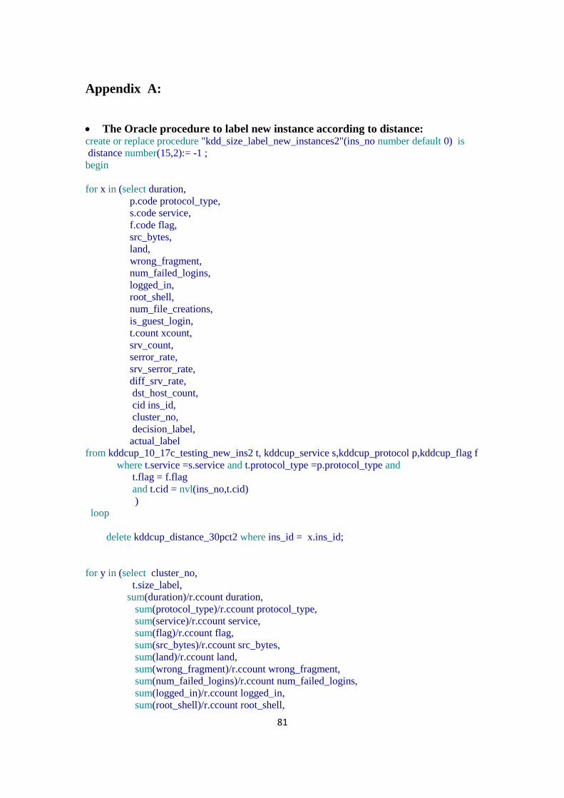
81
Appendix A:
The Oracle procedure to label new instance according to distance: create or replace procedure "kdd_size_label_new_instances2"(ins_no number default 0) is
distance number(15,2):= -1 ;
begin
for x in (select duration,
p.code protocol_type,
s.code service,
f.code flag,
src_bytes,
land,
wrong_fragment,
num_failed_logins,
logged_in,
root_shell,
num_file_creations,
is_guest_login,
t.count xcount,
srv_count,
serror_rate,
srv_serror_rate,
diff_srv_rate,
dst_host_count,
cid ins_id,
cluster_no,
decision_label,
actual_label
from kddcup_10_17c_testing_new_ins2 t, kddcup_service s,kddcup_protocol p,kddcup_flag f
where t.service =s.service and t.protocol_type =p.protocol_type and
t.flag = f.flag
and t.cid = nvl(ins_no,t.cid)
)
loop
delete kddcup_distance_30pct2 where ins_id = x.ins_id;
for y in (select cluster_no,
t.size_label,
sum(duration)/r.ccount duration,
sum(protocol_type)/r.ccount protocol_type,
sum(service)/r.ccount service,
sum(flag)/r.ccount flag,
sum(src_bytes)/r.ccount src_bytes,
sum(land)/r.ccount land,
sum(wrong_fragment)/r.ccount wrong_fragment,
sum(num_failed_logins)/r.ccount num_failed_logins,
sum(logged_in)/r.ccount logged_in,
sum(root_shell)/r.ccount root_shell,

82
sum(num_file_creations)/r.ccount num_file_creations,
sum(is_guest_login)/r.ccount is_guest_login,
sum(t.count)/r.ccount ycount,
sum(srv_count)/r.ccount srv_count,
sum(serror_rate)/r.ccount serror_rate,
sum(srv_serror_rate)/r.ccount srv_serror_rate,
sum(diff_srv_rate)/r.ccount diff_srv_rate,
sum(dst_host_count)/r.ccount dst_host_count
from kddcup_10_17c_testing_30_res t, v_kddcup_10_17c_testing_res_c r
where t.cluster_no = r.dt_cluster_no
group by
cluster_no,
t.size_label,
r.ccount
)
loop
distance := power(power((x.duration - y.duration),2) +
power((x.protocol_type - y.protocol_type),2) +
power((x.service - y.service),2) +
power((x.flag - y.flag),2) +
power((x.src_bytes - y.src_bytes),2) +
power((x.land - y.land),2) +
power((x.wrong_fragment - y.wrong_fragment),2) +
power((x.num_failed_logins - y.num_failed_logins),2) +
power((x.logged_in - y.logged_in),2) +
power((x.root_shell - y.root_shell),2) +
power((x.num_file_creations - y.num_file_creations),2) +
power((x.is_guest_login - y.is_guest_login),2) +
power((x.xcount - y.ycount),2) +
power((x.srv_count - y.srv_count),2) +
power((x.serror_rate - y.serror_rate),2) +
power((x.srv_serror_rate - y.srv_serror_rate),2) +
power((x.diff_srv_rate - y.diff_srv_rate),2) +
power((x.dst_host_count - y.dst_host_count),2) ,0.5);
begin
insert into kddcup_distance_30pct2
(cluster_no, ins_id, distance,cluster_label)
values
( y.cluster_no, x.ins_id, distance,y.size_label);
exception
when others then null;
end;
commit;
end loop;
end loop;
end;

83
create or replace procedure "kdd_size_label_new_instances"(ins_no number default 0) is
distance number(15,2):= -1 ;
begin
for x in (select duration,
p.code protocol_type,
s.code service,
f.code flag,
src_bytes,
land,
wrong_fragment,
num_failed_logins,
logged_in,
root_shell,
num_file_creations,
is_guest_login,
count,
srv_count,
serror_rate,
srv_serror_rate,
diff_srv_rate,
dst_host_count,
cid ins_id,
cluster_no,
decision_label,
actual_label
from kddcup_10_17c_testing_new_ins t, kddcup_service s,kddcup_protocol
p,kddcup_flag f
where t.service =s.service and t.protocol_type =p.protocol_type and
t.flag = f.flag
-- and t.cid = ins_no
and ((t.cid between 100 and 105) or (t.cid between 1600 and 700))
)
loop
delete kddcup_distance_30pct where ins_id = x.ins_id;
for y in (select duration,
protocol_type,
service,
flag,
src_bytes,
land,
wrong_fragment,
num_failed_logins,
logged_in,
root_shell,
num_file_creations,
is_guest_login,
count,

84
srv_count,
serror_rate,
srv_serror_rate,
diff_srv_rate,
dst_host_count,
cid,
cluster_no,
decision_label,
size_label,
decision_info_label,
actual_label
from kddcup_10_17c_testing_30_res)
loop
distance := power(power((x.duration - y.duration),2) +
1+ -- power((x.protocol_type - y.protocol_type),2) +
1+ -- power((x.service - y.service),2) +
1+ -- power((x.flag - y.flag),2) +
power((x.src_bytes - y.src_bytes),2) +
power((x.land - y.land),2) +
power((x.wrong_fragment - y.wrong_fragment),2) +
power((x.num_failed_logins - y.num_failed_logins),2) +
power((x.logged_in - y.logged_in),2) +
power((x.root_shell - y.root_shell),2) +
power((x.num_file_creations - y.num_file_creations),2) +
power((x.is_guest_login - y.is_guest_login),2) +
power((x.count - y.count),2) +
power((x.srv_count - y.srv_count),2) +
power((x.serror_rate - y.serror_rate),2) +
power((x.srv_serror_rate - y.srv_serror_rate),2) +
power((x.diff_srv_rate - y.diff_srv_rate),2) +
power((x.dst_host_count - y.dst_host_count),2) ,0.5);
begin
insert into kddcup_distance_30pct
(cid, cluster_no, ins_id, distance,cluster_label,decision_label)
values
(y.cid, y.cluster_no, x.ins_id, distance,y.size_label,x.decision_label);
exception
when others then null;
end;
commit;
end loop;
end loop;
end;

85
Oracle function to find minimum distance for a new instance.
create or replace function kddcup_30_label_new_instance
(ins_no number) return varchar2 is
begin
for r in ( select x.cluster_no,
x.distance,
x.cluster_label
from (select t.ins_id,
t.cluster_no,
t.cluster_label,
min(t.distance) distance
from kddcup_distance_30pct t
where t.ins_id = ins_no
group by t.ins_id,
t.cluster_no,
t.cluster_label ) x
where x.distance =
(select min(t.distance) distance
from kddcup_distance_30pct t
where t.ins_id = x.ins_id) )
loop
return r.cluster_label;
end loop;
return 'unknown';
end ;
Oracle function to calc detection rate, false alarm and accuracy. create or replace function kdd_evaluation_calc_new return varchar2 is
v_tp number(15) := 0;
v_fp number(15) := 0;
v_fn number(15) := 0;
v_tn number(15) := 0;
tp number(15,2) := 0;
fp number(15,2) := 0;
fn number(15,2) := 0;
tn number(15,2) := 0;
n number := 0 ;
a number := 0 ;
accuracy number(15,2);
detection_rate number(15,2);
false_alarm number(15,2);
begin
for r in ( select sum(vcount) vcount from
kddcup_evaluation_result t
where t.actual_label ='normal' )
loop
n := r.vcount;
end loop;
for r in ( select sum(vcount) vcount from
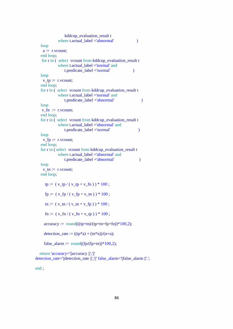
86
kddcup_evaluation_result t
where t.actual_label ='abnormal' )
loop
a := r.vcount;
end loop;
for r in ( select vcount from kddcup_evaluation_result t
where t.actual_label ='normal' and
t.predicate_label ='normal' )
loop
v_tp := r.vcount;
end loop;
for r in ( select vcount from kddcup_evaluation_result t
where t.actual_label ='normal' and
t.predicate_label ='abnormal' )
loop
v_fn := r.vcount;
end loop;
for r in ( select vcount from kddcup_evaluation_result t
where t.actual_label ='abnormal' and
t.predicate_label ='normal' )
loop
v_fp := r.vcount;
end loop;
for r in ( select vcount from kddcup_evaluation_result t
where t.actual_label ='abnormal' and
t.predicate_label ='abnormal' )
loop
v_tn := r.vcount;
end loop;
tp := ( v_tp / ( v_tp + v_fn ) ) * 100 ;
fp := ( v_fp / ( v_fp + v_tn ) ) * 100 ;
tn := ( v_tn / ( v_tn + v_fp ) ) * 100 ;
fn := ( v_fn / ( v_fn + v_tp ) ) * 100 ;
accuracy := round(((tp+tn)/(tp+tn+fp+fn))*100,2);
detection_rate := ((tp*a) + (tn*n))/(n+a);
false_alarm := round((fp/(fp+tn))*100,2);
return 'accuracy='||accuracy ||','||'
detection_rate='||detection_rate ||','||' false_alarm='||false_alarm ||'.';
end ;