Embed Size (px)
Citation preview

Ab-initio Study of Semi-conductor and Metallic
Systems: from Density Functional Theory to
Many Body Perturbation Theory
Master of Science
Zhijun Yi
A thesis submitted for the
degree of Doctor of Science (Dr. rer. nat.)
to the
Department of Physics
University of Osnabruck
October 2009


The work presented in this thesis was accomplished during the time from Octo-
ber 2006 to October 2009 in Prof. Dr. Michael Rohlfing’s group in the Department
of Physics in Universitat Osnabruck.
Supervisor: Prof. Dr. Michael Rohlfing

Contents
1 Introduction 1
2 Density functional theory 7
2.1 Introduction . . . . . . . . . . . . . . . . . . . . . . . . . . . . . . . 7
2.2 Schrodinger equation . . . . . . . . . . . . . . . . . . . . . . . . . . 8
2.3 Thomas-Fermi model . . . . . . . . . . . . . . . . . . . . . . . . . . 9
2.4 Hohenberg-Kohn theorems . . . . . . . . . . . . . . . . . . . . . . . 10
2.5 Kohn-Sham equations . . . . . . . . . . . . . . . . . . . . . . . . . 13
2.6 Local density approximation . . . . . . . . . . . . . . . . . . . . . . 16
2.7 Pseudopotential . . . . . . . . . . . . . . . . . . . . . . . . . . . . . 18
2.8 Optimization method . . . . . . . . . . . . . . . . . . . . . . . . . . 21
2.9 Expansions of Kohn-Sham orbitals . . . . . . . . . . . . . . . . . . 23
2.9.1 Plane wave basis set . . . . . . . . . . . . . . . . . . . . . . 24
2.9.2 Gaussian orbital basis set . . . . . . . . . . . . . . . . . . . 26
2.10 k point samplings . . . . . . . . . . . . . . . . . . . . . . . . . . . . 27
3 DFT study of Si doped GaAs with different charge states 31
3.1 Introduction . . . . . . . . . . . . . . . . . . . . . . . . . . . . . . . 31
3.2 Computational Method . . . . . . . . . . . . . . . . . . . . . . . . . 33
3.3 Results and discussion . . . . . . . . . . . . . . . . . . . . . . . . . 35
3.3.1 DX center in bulk GaAs and in GaAs(110) . . . . . . . . . . 35
3.3.2 Substitutional Si atom in GaAs(110) with different chargestates . . . . . . . . . . . . . . . . . . . . . . . . . . . . . . 40
3.3.3 STM simulation . . . . . . . . . . . . . . . . . . . . . . . . . 43
3.4 Conclusions . . . . . . . . . . . . . . . . . . . . . . . . . . . . . . . 47
4 Many body perturbation theory 48
4.1 Introduction . . . . . . . . . . . . . . . . . . . . . . . . . . . . . . . 48
4.2 The Green’s function . . . . . . . . . . . . . . . . . . . . . . . . . . 50
4.3 Lehmann representation . . . . . . . . . . . . . . . . . . . . . . . . 52
4.4 Spectral function . . . . . . . . . . . . . . . . . . . . . . . . . . . . 55
4.5 Hedin’s equations and the GW approximation . . . . . . . . . . . . 57
4.6 Quasi-particle equations . . . . . . . . . . . . . . . . . . . . . . . . 64
i
Contents ii
5 Quasi-particle bandstructures and lifetimes in metallic systems 66
5.1 Introduction . . . . . . . . . . . . . . . . . . . . . . . . . . . . . . . 66
5.2 Computational details and theoretical methods . . . . . . . . . . . 70
5.3 Quasi-particle band-structures . . . . . . . . . . . . . . . . . . . . 75
5.3.1 Bulk Cu . . . . . . . . . . . . . . . . . . . . . . . . . . . . . 76
5.3.2 Bulk Ag . . . . . . . . . . . . . . . . . . . . . . . . . . . . . 78
5.4 Quasi-particle lifetimes . . . . . . . . . . . . . . . . . . . . . . . . . 80
5.4.1 Bulk Cu . . . . . . . . . . . . . . . . . . . . . . . . . . . . . 80
5.4.2 Bulk Ag . . . . . . . . . . . . . . . . . . . . . . . . . . . . . 84
5.5 Image potential state lifetimes in Cu(100) . . . . . . . . . . . . . . 86
5.5.1 Computational details and discussion of results . . . . . . . 88
5.6 Summary . . . . . . . . . . . . . . . . . . . . . . . . . . . . . . . . 90
A Derivation of some equations in this thesis 91
A.1 The motion of Green’s function . . . . . . . . . . . . . . . . . . . . 91
A.2 Schwinger’s functional derivative . . . . . . . . . . . . . . . . . . . 93
B Detailed information for the pseudopotential generation of Cuand Ag 95
B.1 Pseudopotential generation . . . . . . . . . . . . . . . . . . . . . . . 95
B.2 Gaussian fitting . . . . . . . . . . . . . . . . . . . . . . . . . . . . . 96
Acknowledgements 98
Bibliography 100
Chapter 1
Introduction
With the development of computing facilities, computational materials science has
clearly emerged as an important field of condensed matter physics. In particular,
ab-initio methods are nowadays indispensable for a thorough understanding of
properties and phenomena of materials at the atomic scale. Among these, Kohn-
Sham density functional theory (DFT)[1, 2] in the local density approximation
(LDA)[3] or generalized gradient approximation (GGA)[4, 5] has been the main
tool used by theoreticians for modelling the structural and electronic properties
of materials. The basic idea of DFT is to replace the interacting many-electron
problem with an effective single-particle problems. Therefore the computational
costs were relatively low as compared to the traditional methods which were based
on the complicated many electrons wave functions, such as Hartree-Fock(HF)[6, 7]
theory and its descendants. DFT allows to calculate ground state properties of
large systems: remarkable results have been achieved for ground state properties
of a huge number of systems ranging from atoms and molecules to solids and
surfaces.
A perfect crystal means that every atom of the same type locates in the correct
position. However, most crystalline materials are not perfect: the regular pattern
of atomic arrangement is interrupted by crystal defects. In fact, using the term
”defect” is sort of a misnomer since these features are commonly intentionally used
to manipulate the electronic properties of a material. One of the most important
1
Introduction 2
defect type is the native point defect. A common application of these point defects
is doping of semiconductor crystals, which controls many aspects of semiconductor
behavior. For instance, group IV(e.g. Si, Ge, Sn) atoms taking places of III(e.g.
Ga) atoms or VI(e.g. S, Se,and Te) atoms substituting V atoms(e.g. As) in III-V
semiconductors will introduce extra valence electrons to the semiconductors, and
the excess electrons increase the electron carrier concentration, which is important
for the electrical properties of extrinsic semiconductors. On the experiment side, in
order to obtain direct information about the local environment around the defects,
an approach which has been exploited in the last decade is to cut the material along
a cleavage plane, so that the defects originally inside the crystal are exposed on a
surface, and these defects exposed on a surface or near the surface can be studied
with the scanning tunneling microscopy(STM).
The first part of this work deals with Si doped GaAs. For the surface study
of GaAs, the most interesting plane for GaAs is the (110) surface, which allows
us to obtain usually large atomically flat sufaces without atomic reconstruction.
Although Si doped GaAs systems have been intensively investigated theoretically
and experimentally during the past several decades, a proper description of the
properties of defect in GaAs systems such as the stabilities of charged defects and
the detailed structure around a defect is still an area of active research. Within
theory, these properties of defects can be analyzed from the structural optimization
based on the DFT.
On the other hand, it turns out that the interaction between particles plays
a very implortant role in physical properties. This indicates that the success of
DFT is also accompanied by a number of serious problems. For instance, DFT
underestimates the band gaps of semiconductors and insulators by some tens of
percent due to the simplified treatment of electron-electron interaction. Apart
from the too small gaps, the band dispersions are often reasonable, and hence, a
simple rigid shift can be used to correct the band gaps of semiconductors and insu-
lators. In any case, the DFT errors in s-p metals are probably less significant than
the band gap errors in semiconductors and insulators. Therefore, the experimen-
tal band-structures are often compared with the results of calculations performed

Introduction 3
within DFT. A much more serious problem of DFT arises when it is applied to
calculate the electronic structures of some noble metals. An example is given in
Ref.[8], where large discrepancies between measured Cu band structure and DFT
results have been found. In this case, a simple rigid shift will lead to a ridiculous
result since the band structure of Cu depends on considered band and k point.
Moreover, DFT is mathematically represented by an hermitian hamiltonian, so
that the corresponding single particle states have infinite lifetime.
In order to overcome the above difficulties encountered by DFT, a number of
attempts have been made for improving the DFT. An exact theory for a system
of interacting electrons is based on solving its many body Schrodinger equation.
Unfortunately, the many body Schrodinger equation can not be solved exactly
for most cases due to the nature of the electrons. The better description for
the interacting electrons is to consider them as quasi-particles. The general no-
tion was first introduced by L.D. Landau[9]. Landau’s basic idea was that in a
complicated system of strongly interacting particles, it may be still possible to
describe the properties of the system in terms of the weakly interacting particles.
A many body perturbation theory(MBPT)[10] treatment can deal with a weakly
interacting system of particles, beginning with the non-interacting particles as the
unperturbed state. The MBPT leads to the successful GW approximation(GWA),
developed systematically by Hedin in 1965[11]. Within the MBPT, band energies
can be obtained as the poles of the one-particle Green’s function G, which involve
the electron self-energy Σ(GWA). The self-energy can be formally expanded in
terms of the dynamically screened Coulomb interaction W, the lowest term being
iGW. Due to the high complexity and large computational requirements of many-
body calculations, for a long time the applications of the GWA were restricted
to the electron gas. With the rapid progress in computer power, applications to
realistic materials eventually became possible about two dacades ago. Numerous
applications to semiconductors and insulators reveal that in most cases the GWA
can yield good band structures. The success of the GWA in sp materials has
prompted further applications to some complex metals with localized d electrons.
For instance, full quasi-particle calculations within GW approximation for Ni[12]

Introduction 4
has yielded a good description of band structure, except for the 6 eV satellite.
Another successful calculations for Cu and Ag have been reported in Ref.[13] and
Ref.[14], which are based on the plane wave basis sets. In order to describe prop-
erly the metals with localized d orbitals, one must also consider the contribution
of d electrons to the valence band structure. This indicates that d electrons can
not be frozen into the core part, but must be explicitly included into the valence.
Apart from the d electrons, the semi-core electrons such as 3s and 3p for Cu and 4s,
4p for Ag should be included into the valence[13, 14], since there is a large spatial
overlap with the d electrons for these noble metals. All these will result in a large
number of valence electrons in the calculation, which means large computational
requirements for these metals, especially for calculations using plane wave basis
sets. In this thesis, I will present a full quasi-particle bandstructure calculations
of Cu and Ag using more efficient localized Gaussian basis sets instead of plane
wave basis sets. In addition, it is possible to carry out a surface calculation for the
noble metals within the GW approximation by using a localized Gaussian orbital
basis.
Another interesting study for metals is the quasi-particle excitations, which play
an important role in a rich variety of physical and chemical phenomena[15] such as
energy transfer in photochemical reactions, desorption and oxidation of molecules
at surfaces, spin transport within bulk metals, across interfaces, and at surfaces.
One of the crucial poperties of quasi-particle excitation is their lifetimes which
determine the duration of these excitations. On the experiment side, linewidths
of bulk excited electron states in metals have also been measured, with the use
of photoelectron spectroscopy[16]. A more advanced tool for the study of both
electron and hole lifetimes in the time domain became available by the advent
of the time-resolved two-photon photoemission(TR-2PPE)[17, 18]. Within theo-
retical framework, the early investigations of quasi-particle lifetimes are based on
the free-electron gas(FEG) model of Fermi-liquids[19]. Several other free-electron
calculations of electron-electron scattering rates have also been carried out, for
electron(hole) energies that deviate from the Fermi level, within the random-
phase approximation (RPA)[20, 21] and with inclusion of exchange and correlation

Introduction 5
effects[22, 23]. Nevertheless, detailed TR-TPPE experiments have reported large
deviations of measured hot-electron lifetimes from those predicted within the FEG
model. First-principles calculations of lifetimes in a variety of metals have been
carried out only very recently [24, 25, 26, 27], by using the GW approximation
of many-body theory. Here, I present a first-principles calculation of lifetimes for
noble metals within the GW approximation based on the quasi-particle energies.
The work based on the MBPT deals with bulk Cu, bulk Ag and Cu(100) using
the GW approximation based on the localized Gaussian orbital basis sets.
In Chapter 2, the concept and progress of DFT are introduced. In chapter 3, an
accurate, first-principles study of the electronic structure of Si doped GaAs within
DFT is presented. The plane wave basis used to expand the Bloch wavefunction
requires the use of pseudopotentials. We systematically studied the DX center in
bulk GaAs and in GaAs(110), as well as the relative stability of SiGa defect with
different charge states in different layers of GaAs(110). We report that the DX
center is a metastable state in bulk GaAs and completely unstable in the top few
layers of GaAs(110). Moreover, we found that the Si−Ga defect on the GaAs(110)
surface is more stable compared to Si−Ga defects in the deep layers (below the
surface), while the Si+Ga defect on the GaAs(110) surface is more unstable, as
compared to Si+Ga defects in deep layers. The most interesting finding is that the
extra charge of Si−Ga defect is mainly concentrated on the Si atom when the defect
is exposed on the GaAs(110) surface. In addition, we studied the STM images
of clean GaAs(110) and charged Si:GaAs(110) by employing the Tersoff-Hamann
approximation[28]. The calculated STM images are in good agreement with the
experimental results. We show that at the positive bias voltage the positively
charged Si atom presents a bright feature while the negatively charged Si atom
shows a dark feature.
In Chapter 4, we introduce the MBPT. In chapter 5, We present the calculations
of quasiparticle bandstructures and lifetimes for noble metals Cu and Ag within
the GW approximation. For Cu, both the calculated positions of the d bands and
the width of the d bands is within 0.1 eV compared to the experimental results.
For Ag, partial core correction should be included in the pseudopotential to get

Introduction 6
reliable positions of the d bands. The calculated lifetime agree with the experiment
in the energy region away from the Fermi level, but deviates from the experimental
results near the Fermi level where short range interactions which GWA fails to
describe play an important role. For a better description of the lifetime near
the Fermi level, higher terms beyond the GW approximation in the many body
perturbation theory need to be considered. In addition, the image potential state
lifetimes in Cu(100) have been calculated using GW approximation based on the
localized Gaussian orbital basis sets, and the calculated n=1, 2 image potential
state lifetimes are in good agreement with experimental results.

Chapter 2
Density functional theory
2.1 Introduction
Quantum mechanics (QM) is the correct mathematical description of the behavior
of electrons. In theory, QM can predict any property of an individual atom or
molecule exactly. In practice, the QM equations have only been solved exactly
for few electron systems. A number of methods ranging from semi-empirical to
ab-initio(QM) approaches have been developed for approximating the solution for
many electron systems. The former schemes usually need some parameters which
are taken from or adjusted to experiments. Although semi-empirical calculations
are much faster than their ab initio counterparts, if some parameters for semi-
empirical simulations are not available, or some phenomena of a system are not
yet known, one must rely only on ab initio calculations. The term ab initio is Latin
for ”from the beginning.” This name is given to computations that are derived
directly from theoretical principles with no inclusion of experimental data. The
simplest type of ab initio electronic structure calculation is the Hartree-Fock (HF)
scheme, which is based on a wave function in a form of one Slater determinant.
Though the results of such calculations using HF scheme are reliable, the major
disadvantage is that they are computationally intensive. An alternative scheme is
DFT, which is based on the electron density rather than on the wave functions, and
7

Density functional theory 8
commonly used to calculate the electronic structure of complex systems containing
many atoms such as large molecules or solids. In the following sections I will mainly
introduce DFT, which is based on the ab initio method. DFT has been developed
more recently than other ab initio methods such as Hartree Fock theory and its
descendants.
2.2 Schrodinger equation
An exact theory for a system of ions and interacting electrons is inherently quan-
tum mechanical, which is based on solving a many-body Schrodinger equation of
the form
HkΨk(RI ; ri) = EkΨk(RI ; ri) (2.1)
where H is the hamiltonian of the system. and consists of the following terms
H = −∑I=1
~2
2MI
∇2RI−
∑i=1
~2
2me
∇2ri−
∑Ii
ZIe2
|RI − ri| +1
2
∑
ij(j 6=i)
e2
|ri − rj|
+1
2
∑
IJ(J 6=I)
ZIZJe2
|RI −RJ | (2.2)
In the above equations: Ψk(RI ; ri) is the many body wavefunction that de-
scribes the state of the system; E is the energy of the system; ~ is Planck’s constant
divided by 2π; MI is the mass of ion I; me is the mass of the electron; ZI is the
valence charge of this ion.
In the Eqs. (2.2): the first and second terms are the kinetic energies of ions
and electrons, respectively; Typically, the ions can be considered as moving slowly
in space and the electrons responding instantaneously to any ionic motion due
to the huge difference of mass between ions and electrons(three to five orders
of magnitude), so the quantum-mechanical term for the kinetic energy of the
ions can be omitted, and we take their kinetic energy into account as a classical
contribution. This corresponds to the Born-Oppenheimer approximation. The
Density functional theory 9
third term is the external potential experienced by electrons due to the presence
of the ions; The fourth term is the Coulomb potential between electrons; The last
term is the potential between ions(Madelung energy of the ions), which as far as
the electron degrees of freedom are concerned is simply a constant. Finally, the
hamiltonian of the system can be reduced to the following terms
H = −∑i=1
~2
2me
∇2ri−
∑Ii
ZIe2
|RI − ri| +1
2
∑
ij(j 6=i)
e2
|ri − rj| (2.3)
Even with this simplification, however, solving for Ψk(ri) is an extremely dif-
ficult task, because of the nature of the electrons. If two electrons of the same spin
interchange positions Ψk(ri) must change sign; this is known as the ”exchange”
property, and is a manifestation of the Pauli exclusion principle. Moreover, each
electron is affected by the motion of every other electron in the system; this is
known as the ”correlation” property. Accurate results can be obtained for the
energy levels and wave functions of two-electron atom by performing variational
calculations. But this method becomes increasingly tedious when the number of
the electrons increases in the atomic system. It is possible to produce a simpler,
approximate picture, in which we describe the system as a collection of classi-
cal ions and essentially single quantum mechanical particles that reproduce the
behavior of the electrons: this is the single-particle picture.
2.3 Thomas-Fermi model
In order to deal with many-electron systems, the Thomas-Fermi model was de-
veloped by Thomas and Fermi [29, 30] in 1927 after the introduction of the
Schrodinger equation. This is the original DFT of quantum systems. In this
model, a statistical model was employed to approximate the distribution of elec-
trons in an atom. The basic idea in this approach is that electrons are distributed
uniformly in phase space, and have no interacting with each other. Finally, the

Density functional theory 10
kinectic energy was expressed as a functional of the electron density
TTF [ρ] = CF
∫ρ
53 (r)dr (2.4)
where CF = 310
(3π2)23 , CF · ρ 5
3 is the kinetic energy density of the non-interacting
homogeneous electron gas.
Combining this kinetic energy term with the classical expressions for the nucleus-
electron and electron-electron interactions, which can both also be represented in
terms of the electron density, the total energy of system can be expressed as
ETF [ρ] =3
10(3π2)
23
∫ρ
53 (r)dr−Z
∫V (r)ρ(r)dr+
1
2
∫ ∫ρ(r1)ρ(r1)
|r1 − r2| dr1dr2 (2.5)
where Z is nuclear charge. Although the TF model represents a drastic approx-
imation of the N-electron problem, it is very useful for the description of the
general trends in the properties of atom. However, using the approximation
for realistic systems more complex than an isolated atom yield poor quantita-
tive predictions[31]. Nevertheless, introducing the one particle electron density to
many-body systems was an important step for the calculations of many-electron
systems, and the more sophisticated and accurate Hohenberg-Kohn theorems[32]
were developed based on this idea.
2.4 Hohenberg-Kohn theorems
The name of DFT was called formally after the publication of two original papers
of Hohenberg, Kohn and Sham[1, 32], referred to as the Hohenberg-Kohn-Sham
theorem. Similar to Hartree-Fock theory[6, 7], DFT introduces three approx-
imations: Born-Oppenheimer approximation, non-relativitic approximation and
single-particle approximation. The largest error for the Hartree-Fock method is
the single-particle approximation, and this can be reduced by the DFT. This the-
ory has a tremendous impact on realistic calculations of the properties of molecules

Density functional theory 11
and solids, and its applications to different problems continue to expand. A mea-
sure of its importance and success is that its main developer, W. Kohn (a theo-
retical physicist) shared the 1998 Nobel prize for Chemistry with J.A. Pople (a
computational chemist). We will review here the essential ideas behind DFT.
Let us consider a system of N interacting electrons in a non-degenerate ground
state associated with an external potential V (r).
Lemma 1. The ground state density, ρ(r), uniquely determines the potential
V (r), within an additive constant.
In order to prove this, assume that two different external potentials, V (r) and
V ′(r), give rise to the same charge density ρ(r). I will show that this postulate is
wrong.
The Hamitonian of a system is given by
H = T + V + W (2.6)
where the T is the kinetic energy operator , W represents the electron-electron
interaction operator and V denotes the external potential operator.
For a system with the kinetic energy T and the electron-electron interaction W,
we assume that V (r) and V ′(r) do not differ merely by a constant. Let E and
Ψ be the total energy and wavefunction and E ′ and Ψ′ be the total energy and
wavefunction for the system with Hamitonion H and H ′, respectively.
H = T + V + W (2.7)
and
H ′ = T + V ′ + W (2.8)

Density functional theory 12
Using the variational principle,
E < 〈Ψ′|H|Ψ′〉 = 〈Ψ′|H ′ + H − H ′|Ψ′〉= 〈Ψ′|H ′|Ψ′〉+ 〈Ψ′|V − V ′|Ψ′〉= E ′ +
∫ρ(r)[V (r)− V ′(r)]dr (2.9)
Similarly we can prove
E ′ < E −∫ρ(r)[V (r)− V ′(r)]dr (2.10)
adding above two equations, we obtain
(E + E ′) < (E + E ′) +
∫ρ(r)[V (r)− V ′(r)]dr−
∫ρ(r)[V (r)− V ′(r)]dr (2.11)
The sum of last two terms on the right hand-side is zero. Finally, we obtain the
following relation
(E + E ′) < (E + E ′) (2.12)
This is a contradiction, therefore we conclude that the assumption about the
densities being the same is not correct. This proves that the ground state density
uniquely determines the external potential V (r), within an additive constant. So
we conclude that the total energy of the system is a functional of the density, and
is given by
E[ρ(r)] = 〈Ψ|H|Ψ〉 = F [ρ(r)] +
∫V (r)ρ(r)dr (2.13)
where F [ρ(r)] represents 〈Ψ|T + W |Ψ〉.
The energy functional can be expressed as
E[ρ] = F [ρ] + V [ρ] = T [ρ] + V [ρ] +W [ρ] (2.14)
Therefore, the first theorem can be summarized by saying that the energy is a
functional of the density. The second theorem establishes a variational principle:

Density functional theory 13
Lemma 2. The ground state energy can be obtained variationally: the density
that minimises the total energy is the exact ground state density.
The proof of the second theorem is also simple. According to theorem 1, a system
with ground state density ρ0(r) determines uniquely its own external potential
V (r) and ground state wave function Ψ0
E[ρ0(r)] = 〈Ψ0|H|Ψ0〉 = F [ρ0(r)] +
∫V (r)ρ0(r)dr (2.15)
Now consider any other density ρ′(r), which necessarily corresponds to a different
wave function wave function Ψ′. This would lead to
E[ρ′(r)] = 〈Ψ′|H|Ψ′〉 = F [ρ′(r)] +∫V (r)ρ′(r)dr > 〈Ψ0|H|Ψ0〉 = E[ρ0(r)] (2.16)
Thus the energy given by the eaquation 2.15 in terms of the Hohenberg-Kohn
functional evaluated for the correct ground state density ρ0(r) is indeed lower
than the value of this expression for any other density ρ′(r).
It follows that if the functional F [ρ(r)] was known, then by minimizing the total
energy of the system, with respect to variations in the density function ρ0(r), one
would find the exact ground state density and energy. Note that the functional
only determines the ground state properties; it does not provide any guidance
concerning excited states.
2.5 Kohn-Sham equations
The Hohenberg-Kohn theorem offers no practical guide to the explicit construction
of the F [ρ(r)] universal functional. For this purpose one still has to face the full
intricacies of the many-body problem. Although there are some energy functionals
for Coulomb systems derived with the theory of the homogeneous electron gas or
in other more elaborated approaches, the situation cannot be considered satisfac-
tory. Only with the approach introduced by Kohn and Sham[1] has been able

Density functional theory 14
to calculate (not only) ground state properties of many-particle Coulomb systems
with great accuracy.
In the following discussion we will define the density ρ(r) and the one-particle
and two-particle denstiy matrices, denoted by γ(r, r′), Γ(r, r′|r, r′), respectively,
as expressed through the many-body wavefunction:
ρ(r) = N
∫Ψ∗(r, r2, · · · , rN)Ψ(r, r2, · · · , rN)dr2 · · · drN (2.17)
γ(r, r′) = N
∫Ψ∗(r, r2, · · · , rN)Ψ(r′, r2, · · · , rN)dr2 · · · drN (2.18)
Γ(r, r′|r, r′) =N(N − 1)
2
∫Ψ∗(r, r′, r3, · · · , rN)Ψ(r, r′, r3, · · · , rN)dr3 · · · drN
(2.19)
From the form of Eqs.(2.14) the energy functional contains three terms: the
kinetic energy T [ρ], the external potential V [ρ] and the electron-electron inter-
action W [ρ]. The kinetic and electron-electron functionals are unknown. Using
the expressions for the one-particle and two-particle denstiy matrices, the explicit
expression for E[ρ] can be written as
E[ρ(r)] = 〈Ψ|H|Ψ〉 = − ~2
2m
∫∇2γ(r, r′)|r′=rdr
+
∫ ∫e2
|r− r′|Γ(r, r′|r, r′)drdr′ +∫V (r)γ(r, r)dr (2.20)
Kohn and Sham[1] proposed a good approximation for reducing these expressions
to a set of single-particle equations. They introduced a fictitious system of N
noninteracting electrons to be described by the single-particle orbitals φi that
appear in the Slater determinant. In this system the one-particle and two-particle
denstity are known exactly from the orbitals:
ρ(r) =∑
i
|φi(r)|2 (2.21)
γ(r, r′) =∑
i
φ∗i (r)φi(r′) (2.22)

Density functional theory 15
Γ(r, r′|r, r′) =1
2[ρ(r)ρ(r′)− |γ(r, r′)|2] (2.23)
With the help of above equations, the energy functionals of Eqs. (2.20) can take
the following form
E[ρ(r)] = T S[ρ(r)] +e2
2
∫ ∫ρ(r)ρ(r′)|r− r′| drdr
′ +∫V (r)ρ(r) + EXC [ρ(r)] (2.24)
In this expression, the first term represents the kinetic energy in the Slater de-
terminant(i.e. this is not the true kinetic energy but is that of a system of non-
interacting electrons, and hence the superscipt S). Since the fictitious particles are
non-interacting, the kinetic energy can be known exactly, and take the following
form
T S[ρ(r)] =∑
i
〈φi| − ~2
2m∇2
r|φi〉 (2.25)
The second term VH [ρ(r)] in Eqs. (2.24) is the bare Coulomb interaction( this
term is seperated out from the electron-electron interaction term Vee[ρ(r)] in Eqs.
(2.20)); The last term in Eqs. (2.24) denotes the exchange-correlation term, which
is simply the sum of the error made in using a non-interacting kinetic energy
and the error made in treating the electron-electron interaction classically, and is
expressed as
EXC [ρ(r)] = (T [ρ(r)]− T S[ρ(r)]) + (Vee[ρ(r)]− VH [ρ(r)]) (2.26)
With the restriction condition∫ρ(r)dr = N , applying the variational principle
δ(E − εi∫ρ(r)dr)
δφi
=δ(E − εi
∫ρ(r)dr)
δρ
δρ
δφi
= 0 (2.27)
to Eqs. (2.24) , we arrive at the following single-particle equation through a
variational argument
[− ~2
2m∇2
r + V (r) + e2∫
ρ(r′)|r− r′
dr′ + VXC(ρ)]φi = εiφi (2.28)
where εi is the Lagrange multiplier, and a local multiplicative potential is intro-
duced, which is the functional derivative of the exchange correlation energy with

Density functional theory 16
respect to the density:
VXC [ρ] =δEXC [ρ(r)]
δρ(r)(2.29)
The single particle Eqs. (2.28) is the well known Kohn-Sham equation with the
resulting density ρ(r) and total energy E given by Eqs. (2.21) and Eqs. (2.24). The
single particle orbitals φi that are their solutions are called Kohn-Sham orbitals.
Kohn-Sham equation describes the behavior of non-interacting ”electrons” in an
effective local potential, which can be expressed as
V eff [r, ρ(r)] = V (r) + e2
∫ρ(r′)|r− r′
dr′ + VXC(ρ) (2.30)
The effective potential is a function of the density, and hence depends on all the
single-particle states. KS results from the Hohenberg-Kohn theorems that the
ground state denstity uniquely determines the potential at the minimum(except
for a trivial constant), so that there is a unique KS potential Veff (r)|min = VKS(r)
associated with any given interacting electron system. We will need to solve these
equations by iteration until we reach self-consistency, but this is not a significant
problem. For the iteration, an initial charge density is needed. To obtain the
charge density, an initial ”guess” to the Kohn-Sham orbitals is needed. This
initial guess can be obtained from a set of basis functions whereby the coefficients
of expansion of the basis functions can be optimized. A more pressing issue is
the exact form of EXC [ρ(r)]. In the following section I will discuss the exchange-
correlation functionals.
2.6 Local density approximation
In principle, the solution of the Kohn and Sham Eqs. (2.28) with the exact
exchange-correlation potential would give a set of fictious single particle eigenstates
whose density of states equals that of the fully interacting system. Unfortunately,
the exact exchange-correlation potential is not yet known. In practice, it is neces-
sary to make approximations for this term. The generation of approximations for
EXC [ρ(r)] has lead to a large and still rapidly expanding field of research. There
Density functional theory 17
are now many different flavours of approximation for the exchange-correlation po-
tential. One of the most widely used is the Local Density Approximation(LDA).
Many approaches can yield local approximations to the XC energy. Overwhelming,
however, successful local approximations are those that have been derived from
the homogeneous electron gas (HEG) model. The principle of this approximation
is to calculate the exchange and correlation energies per particle εXC [ρ(r)], of the
homogeneuos electron gas as a function of the density:
EXC [ρ(r)] =
∫εXC [ρ(r)]ρ(r)dr (2.31)
where ρ(r) is the electronic density. This approximation is based on the assumption
that the system locally appears as an homogeneous electron gas. The exchange-
correlation energies per particle εXC [ρ(r)] can be seperated into exchange and
correlation contributions:
εXC [ρ(r)] = εX [ρ(r)] + εC [ρ(r)] (2.32)
While εX [ρ(r)] is an analytic function of ρ(r)[33]
εX [ρ(r)] = −3
4e2(
3
πρ(r))
13 (2.33)
The functional form for the correlation energy density εC [ρ(r)] is unknown
and has been simulated for the homogeneous electron gas in numerical quantum
Monte Carlo calculations which yield essentially exact results (Ceperley and Alder,
1980)[3]. Various approaches, using different analytic forms for εC [ρ(r)], have gen-
erated several LDA’s for the correlation functional, including: Vosko-Wilk-Nusair
(VWN)[34], Perdew-Zunger (PZ81)[35], Cole-Perdew (CP)[36] and Perdew-Wang
(PW92)[37]. All of these yield similar results in practice and are collectively re-
ferred to as LDA functionals.
The LDA has proven to be a remarkably fruitful approximation. Properties
such as structure, vibrational frequencies, elastic moduli and phase stability (of
similar structures) are described reliably for many systems. For this reason, the

Density functional theory 18
LDA has been employed to describe the structure of GaAs(110) systems in the
next chapter.
The common feature in this approach is that EXC [ρ(r)] depends on ρ(r) in
a local fashion, that is, ρ(r) needs to be evaluated at one point in space at a
time. For this reason they are referred to as the Local Density Approximation to
Density Functional Theory. This is actually a severe restriction, because even at
the exchange level, the functional should be non-local, that is, it should depend
on r and r′ simultaneously. It is a much more difficult task to develop non-local
exchange-correlation functionals. More recently, a concentrated effort has been
directed toward producing expressions for EXC [ρ(r)] that depend not only on the
density ρ(r), but also on its gradients[4, 5]. These expansions tend to work better
for some cases, but still represent a local approximation to the exchange-correlation
functional. More advanced method for the evaluation of the exchange-correlation
part is based on the many body perturbation theory[10], which will be introduced
in the third chapter.
2.7 Pseudopotential
Electrons in matter can be broadly categorised into two types: core electrons,
which are strongly localized in the closed inner atomic shells, and valence electrons,
which also extend outside the core. If core electrons are included completely in the
calculation, a large number of basis functions(especially if a plane wave basis set
is used) would be required due to the oscillations in the core regions which main-
tain orthogonality between valence and core electrons. As a result, all electron
calculations demand a huge computational expense that is simply not practical.
On the other hand, by realising that the electronic structure of the core-electrons
remains largely unchanged in different chemical environments, and is also of mini-
mal interest generally, the problems relating to the core-electrons can be overcome
by use of the pseudopotential approximation. In this approach the ionic potential
Vion(r) in the core region is replaced by a weaker pseudopotential vPSion(r). The

Density functional theory 19
Figure 2.1: Schematic illustration of the pseudopoential concept. The solidlines show the all-electron wavefunction, ΨAE(r) and ionic potential,vAE
ion (r),while the dashed lines show the corresponding pseudo-wavefunction, ΨPS(r),given by the pseudopotential,vPS
ion(r). All quantities are shown as a functionof distance, r, from the atomic nucleus. The cutoff radius rc marks the point
beyond which the all-electron and pseudo-quantities become identical.
corresponding set of pseudo-wavefunctions ΨPS(r) and the all-electron wave func-
tions ΨAE(r) are identical outside a choosen cutoff radius rc and so exhibit the
same scattering properties, but ΨPS(r) does not possess the nodal structure that
cause the oscillations inside rc. A schematic illustration of the pseudopotential
concept is shown in Fig. 2.1. The choice of the rc is very important. In general,
the larger rc will result in a softer pseudopotential(less cpu time in practical cal-
culation), but also the less transferable. There is no well-defined answer for how
to choose a rc. In practice, rc should be larger than the outermost node(if any) of
the wavefunction for any given angular momentum. Usually there is one angular
momentum that is harder than the others (in transition metals, the d state, in
second-row elements N, O, F, the p state), and one should concentrate on this one
and push outwards its rc as much as possible. In addition, one should try to have
not too different rc for different angular momenta.
The majority of pseudopotentials used in DFT calculations are generated from
all-electron atomic calculations by self-consistently solving the following radial

Density functional theory 20
Schrodinger equation,
[−1
2
d2
dr2+l(l + 1)
2r2− Z
r+ VH(r) + VXC(r)]ψAE
l (r) = εlψAEl (r) (2.34)
where VH(r) and VXC(r) are the Hartree and exchange-correlation potentials, and
ψAEl (r) is the all-electron atomic wavefunction with angular momentum compo-
nent l. Conventionally, the pseudopotential is then constructed by satisfying four
general criteria: (i) the valence pseudo-wavefunction ψPSl (r) must be the same as
ψAEl (r) outside a given cutoff radius rc, (ii) the charge enclosed within rc must be
equal for the two wavefunctions,
∫ rc
0
r2|ψPSl (r)|2dr =
∫ rc
0
r2|ψAEl (r)|2dr = 1 (2.35)
This is commonly referred to as norm-conservation. (iii) ψPSl (r) must not contain
any nodes and be continuous at rc, as well as its first and second derivatives.
Finally, (iv)the valence eigenvalues from all-electron and pseudopotential must be
equal.
The pseudopotential is not uniquely constructed, indeed the above conditions
permit a considerable amount of freedom when generating pseudo-wavefunctions,
consequently many different ways have been developed for constructing pseudopo-
tentials. Once a particular pseudo-wavefunction is created, the ionic pseudopo-
tential is then obtained by inverting the radial Kohn-Sham Eqs. (2.34), giving,
V PSion,l(r) = εl − V PS
H (r)− V PSXC (r)− l(l + 1)
2r2+
1
2ψPSl (r)
d2ψPSl (r)
dr2(2.36)
where V PSH (r) and V PS
XC (r) are calculated from pseudo-wavefunctions. A conse-
quence of this procedure is that a seperate pseudopotential must be generated for
each angular momentum component l. The pseudopotential operator V PS(r) can
be written in a semi-local form[38, 39] as
V PSion (r) = V PS
loc (r) +∑
l
δV PSl (r)Pl (2.37)

Density functional theory 21
where V PSloc (r) is a local potential and Pl projects out the lth angular momentum
component of the semi-local part δV PSl (r)
δV PSl (r) = V PS
ion (r)− V PSloc (r) (2.38)
Kleinman and Bylander[KB][40] observed that greater efficiency could be attained
if the non-locality was not restricted to the angular momentum part, but if the
radial component was also converted into a separable non-local form. Therefore in
the Kleinman-Bylander approach, the semi-local form is converted into the fully
non-local form δV PSKB(r), given by,
δV PSKB(r) =
∑
l
|δV PSl (r)φ0
l (r)〉〈φ0l (r)δV
PSl (r)|
〈φ0l (r)|δV PS
l (r)|φ0l (r)〉
(2.39)
where the φ0l (r) are the atomic pseudo-wavefunctions calculated with δV PS
l (r).
The Kleinman-Bylander form drastically reduces the computational resources in
a pseudopotential calculation: for a plane-wave expansion of dimensionality NPW ,
the semi-local form requires storage of v (N2PW +NPW )2 projections for each
angular momentum state, whereas the corresponding KB pseudopotential evalu-
ates just NPW projections and simple multiplications.
2.8 Optimization method
In the beginning of the calculations atomic coordinates are either from experiments
or classical simulations. Unfortunately, these atomic coordinates are usually not at
equilibrium within DFT. Therefore, it is necessary to optimize the atomic coordi-
nates. There are many optimization methods for first-principles calculations. Al-
most all optimization codes use what is called a quadratic approximation, namely
they expand the dependence of energy in a form
E∗ = E + gT s +1
2sTBs (2.40)

Density functional theory 22
where E∗ is the predicted energy for a step s from the current point; B is the Hes-
sian matrix. E and g are the energy and gradient(negative of the force) calculated
at the current point. According to the Hellmann-Feynman theorem [42, 43], the
force can be expressed as
f = − d
dR〈Ψ|H|Ψ〉 = −〈Ψ|∂H
∂R|Ψ〉 (2.41)
where R denotes the atomic positions, and H is the hamiltonian of the system.
For the evaluation of the Hessian matrix, different algorithm use different ap-
proaches to this matrix. The most primitive is steepest descent, which takes B
as the unitary matrix so the algorithm will take a step along the direction of the
force. Better algorithms such as conjugate gradient methods use some information
about the previous step. By far and away the most common method is to exploit
the Hessian, either by directly computing it (very CPU expensive for codes) or to
create an estimate of it that improves as the calculation proceeds. The most suc-
cessful approach is the Broyden-Fletcher-Goldberg-Shamo (BFGS)[41] update. In
mathematics, the BFGS method is a method to solve an unconstrained nonlinear
optimization problem. The BFGS method is derived from the Newton’s method
in optimization, a class of hill-climbing optimization techniques that seeks the sta-
tionary point of a function, where the gradient is zero. Newton’s method assumes
that the function can be locally approximated as a quadratic form in the region
around the optimum, and use the first and second derivatives to find the stationary
point. In Quasi-Newton methods the Hessian matrix of second derivatives of the
function to be minimized does not need to be computed at any stage. The Hessian
is updated by analyzing successive gradient vectors instead. Quasi-Newton meth-
ods are a generalization of the secant method to find the root of the first derivative
for multidimensional problems. In multi-dimensions the secant equation is under-
determined, and quasi-Newton methods differ in how they constrain the solution.
The BFGS method is one of the most successful members of this class, and I will
give a very brief introduction to this optimization method.

Density functional theory 23
If we take a step sk, the gradient will change from gk at the previous point to
gk+1 at the new point, and we can write
gk − gk+1 = yk = Bksk (2.42)
In principle, there are many ways to exploit this information. The method used
in BFGS is to update the Hessian for the next step via:
Bk+1 = Bk + ∆Bk (2.43)
∆Bk = −ykyTk
sTk yk
+Bksks
Tk Bk
sTk Bksk
(2.44)
The procedure is then to solve for
sk+1 = −B−1k+1gk (2.45)
move by sk+1, recalculate the gradient,update the Hessian Bk and iterate. Often
the first estimate for the Hessian is the unitary matrix, although it does not have
to be and the better the initial guess is, the faster the algorithm will converge.
Often the estimate of the Hessian will change rather a lot during the calculation,
and at some locations can be rather bad. The power of the BFGS method is that
experience over the last decade has indicated that in most cases it will correct
itself rather quickly, and is therefore rather robust.
2.9 Expansions of Kohn-Sham orbitals
All ab initio electronic structure calculations employ expansions in basis sets of
atomic orbitals. The two most common choices of basis function are plane waves
and Gaussian type.

Density functional theory 24
2.9.1 Plane wave basis set
As yet there has been no mention of how to handle the infinite number of interact-
ing electrons moving in the static field of an infinite number of ions. Essentially,
there are two difficulties to overcome: a wavefunction has to be calculated for each
of the infinite number of electrons which will extend over the entire space of the
solid and the basis set in which the wavefunction will be expressed will be infinite.
The ions in a perfect crystal are arranged in a regular periodic way (at 0K).
Therefore the external potential felt by the electrons will also be periodic - the pe-
riod being the same as the length of the unit cell L(That is, the external potential
on an electron at r can be expressed as V (r) = V (r+L)). This is the requirement
needed for the use of Bloch’s theorem. By the use of this theorem, it is possible
to express the wavefunction of the infinite crystal in terms of wavefunctions at
reciprocal space vectors of a Bravais lattice. The Bloch theorem states that wave-
function of an electron Ψik(r), within a periodic potential, can be written as the
product of a lattice periodic part uik(r) and a wavelike part exp(ik · r),
Ψik(r) = exp(ik · r)uik(r) (2.46)
where the subscript i indicates the band index and k is in the first Brillouin
zone(BZ) and periodic; uik(r) can be expanded in a Fourier series :
uik(r) =∑
G
ci,Gexp(iG · r) (2.47)
where ci,G is the coefficient in the expansion. The above results show that the
electron wavefunctions can be expanded in terms of a linear combination of plane
waves,
Ψik(r) =∑
G
ci,k+Gexp(i(k + G) · r) ≡∑q
ci,q|q〉(q = k + G) (2.48)
By the use of Bloch’s theorem, the problem of the infinite number of electrons
has now been mapped onto the problem of expressing the wavefunction in terms

Density functional theory 25
of an infinite number of reciprocal space vectors within the first Brillouin zone of
the periodic cell, k. This problem is dealt with by sampling the Brillouin zone at
special sets of k-points discussed in Section 2.10. The electronic wavefunctions at
each k-point are now expressed in terms of a discrete plane wave basis set, which
offers a complete basis set that is independent of the type of crystal and treats
all areas of space equally. This is in contrast to some other basis sets which use
localised functions such as Gaussians which are dependent on the positions of the
ions.
Using a plane-wave basis set to expand the electronic wavefunctions in periodic
systems leads to a particularly simple formulation of the Kohn-Sham equations in
DFT. Accounting for the fact that the potential has the same lattice periodicity
as uik(r)
Veff (r) =∑
G
Veff (G)exp(iG · r) (2.49)
One arrives at the following expression for its matrix elements in the plane-wave
basis:
〈q′|Veff (r)|q〉 =∑
G
Veff (G)〈q′|exp(iG · r)|q〉 =∑
G
Veff (G)δq′−q,G (2.50)
Substituting these Bloch states into the Kohn-Sham equations, multiplying by 〈q′|from the left and integrating over r gives a set of matrix equations for any given k
∫dr〈q′|[−1
2∇2 + Veff (r)]
∑q
ci,q|q〉 = εici,q|q〉 (2.51)
Finally, we obtain a reciprocal-space representation of the Kohn-Sham equations,
∑
G′[1
2|k + G|2δG,G′ + Veff (G−G′)]ci,k+G′ = εici,k+G (2.52)
For an exact calculation, the dimension of the plane-wave basis set should be
infinite. Fortunately the plane-waves at the lower end of the kinetic energy range
are most important, so a practical solution of KS equation can be obtained by
truncating the basis set to a finite number of plane-waves. This is defined by the

Density functional theory 26
kinetic cutoff energy Ecut,1
2|k +G|2 ≤ Ecut (2.53)
Certain integrals and operations are much easier to carry out with plane wave
basis functions, than with their localized counterparts. In practice, plane wave
basis sets are often used in combination with pseudopotential, so that the plane
waves are only used to describe the valence charge density. This is because core
electrons tend to be concentrated very close to the atomic nuclei, resulting in large
wavefunction and density gradients near the nuclei which are not easily described
by a plane wave basis set unless a very high energy cutoff, (and therefore small
plane wavelength), is used. Furthermore, all functions in the basis are mutually
orthogonal, and plane wave basis sets do not exhibit basis set superposition error.
Another important advantage of a plane wave basis is that it is guaranteed to
converge to the target wave function if Ecut →∞ while there is no such guarantee
for Gaussian type basis sets.
2.9.2 Gaussian orbital basis set
There are also some disadvantages with plane wave expansions. The principal
of these is that an extremely large number of functions need to be used for the
systems, expecially for some metals with localized d orbitals. This means that the
time and memory requirements of such a code will be considerable. One way of
avoiding this is to use a basis set of localised orbitals, such as Gaussian orbitals:
ψi,k(r) =∑
i
Ciφi(r) (2.54)
φi(r) =1√Ω
∑R
exp(ik · (R + τi))fi(r−R− τi) (2.55)
where
fi(r) = xn1yn2zn3Ylm(θ, ϕ)exp(−βr2) (2.56)
Ylm(θ, ϕ) are spherical harmonics. The atomic position in the unit cell is τi and
R is a Bravais lattice vector. n1, n2 and n3 are integers, and specifies the orbital

Density functional theory 27
character(n1 + n2 + n3 = l). If n1, n2 and n3 are all zero the function corresponds
to a s orbital of spherical symmetry. Orbitals of p-symmetry correspond to one of
these integers being unity and the others zero, whereas five d-like and one s-like
orbital can be generated if n1 + n2 + n3 = 2.
This expansion has the advantage that it is very efficient, efficiently applicable
to all elements of the periodic table, and it is flexible (if we have one difficult
atom, additional orbitals can be placed on just that atom so the overall speed
of the calculation is not significantly affected). For example when modelling an
element of a transition element as an impurity in silicon, higher angular momentum
functions need to be placed on that atom. However, the rest of the system can be
treated with the standard basis set.
Disadvantages include the fact that the functions can become over-complete
(numerical noise can enter a calculation if two functions with similar exponents
are placed on the same atom), that they are difficult to program (especially if
high angular momentum functions are needed), that it is difficult to test or to
demonstrate absolute convergence (many things can be changed: the number of
functions, the exponents, the function centres).
2.10 k point samplings
The first Brillouin zone can be mapped out by a continuous set of points, through-
out that region of reciprocal space (k-space). The occupied states at each k-point
contribute to the electronic potential of the bulk solid. Since the set k is dense,
there are an infinite number of k-points in the Brillouin zone at which the wave-
functions must be calculated. Therefore if a continuum of basis sets were required,
the basis set for any calculation would still be infinite.
For this reason electronic states are only calculated at a set of k-points deter-
mined by the shape of the Brillouin zone compared to that of its irreducible part.
The reason that this can be done is that the electronic wavefunctions at k-points

Density functional theory 28
that are very close to each other will almost be identical. It is therefore possible to
represent the electronic wavefunctions over a region of reciprocal space at a single
k-point. This approximation allows the electronic potential to be calculated at a
finite number of k-points and hence determine the total energy of the solid.
Methods have been devised for obtaining very accurate approximations to the
electronic potential from a filled electronic band by calculating the electronic wave-
functions at special sets of k-points. The two most common methods are those of
Chadi and Cohen[44] and Monkhorst and Pack[45]. I will mainly introduce the
method of Chadi and Cohen, which has been employed for all calculations in this
thesis.
We consider a smoothly varying periodic function, and expand it in a Fourier
series:
g(k) = f0 +∞∑
i=m
gmeik·Rm (2.57)
where the Rm are lattice vectors. Let us assume another function f(k) which has
the complete symmetry T of the lattice:
f(k) =1
nT
∑i
g(Tik) (2.58)
where Ti range over all the operations of the lattice point group T , and nT is the
number of elements in T . From g(k) we can express f(k) in the following form
f(k) = f0 +∞∑
m=1
∑i
1
nT
gmeiTik·Rm
= f0 +∞∑
m=1
fmAm(k) (2.59)
where
fm =gm
nT
, (2.60)
and
Am(k) =∑
|R|=Cm
eik·Rm (2.61)
Density functional theory 29
In the above equation, the lattice vectors are ordered, and satisfy 0 < Cm ≤ Cm+1.
Am(k) satisfies the following relations:
Ω
2π3
∫
BZ
Am(k)dk = 0, m = 1, 2, . . . (2.62)
Ω
2π3
∫
BZ
Am(k)An(k)dk = Nnδmn (2.63)
Am(k + G) = Am(k) (2.64)
Am(Tik) = Am(k) (2.65)
Am(k)An(k) =∑
j
aj(mn)Aj(k) (2.66)
In the above equations Ω is the volume of the primitive cell, Nn is the number of
lattice vectors, and G is any lattice reciprocal lattice vector. The average value
over the Brillouin zone of the f is given by
f =Ω
2π3
∫f(k)dk (2.67)
Inserting Eqs. (2.59) into above equation, we can obtain f = f0. The perfect
special k-points, k0, would have Am(k0) = 0 for m = 1, 2, · · · ,∞, so that f =
f0 = f(k0). This point is called the ” mean value point”. In fact, such a point does
not exist. The expansion coefficients fm values markedly decrease for larger m so
that the equation Am(k0) = 0 should be satisfied for a finite value of m. As the
Am(k) only depend on the lattice vectors, they can be determined for each crystal
structure, independent of the actual function f(k) that one wants to evaluate.
Baldereschi [46] has obtained for the cubic crystals the point k0, which satisfies
Am(k0) = 0 for a finite value of m, and yielded good electron charge density and
energy in a number of diamond and zinc-blende crystals.
In order to satisfy the relation Am(k0) = 0 for large values of m, one can choose
a sequence of sets of points k and associated weights W which satisfy the
conditionsn∑
i=1
WiAm(ki) = 0,m = 1, 2, · · · , N (2.68)

Density functional theory 30
where N is a finite value.n∑
i=1
Wi = 1 (2.69)
Using Eqs. (2.59), one can obtain
n∑i=1
Wif(ki) = f0
n∑i=1
Wi +N∑
m=1
n∑i=1
WiAm(ki)fm +∞∑
m=N+1
n∑i
WiAm(ki)fm (2.70)
Using Eqs. (2.69) and Eqs. (2.68), the above equation takes the following form
f0 =n∑
i=1
Wif(ki)−∞∑
m=N+1
n∑i
WiAm(ki)fm (2.71)
Since the expansion coefficients fm decrease rapidely for larger m, if N is large
enough, we can neglect the second term of the above equation, and obtain the
following relation
f0 =n∑
i=1
Wif(ki) (2.72)
Therefore, the average value over the Brillouin zone of the f can be represented
by a special set of k-points.
The fact is used by Chadi and Cohen to generate a special set of k-points
at which the reciprocal space should be sampled. The k-point set is generated
as follows: picking two starting k-points k1 and k2 satisfying certain uniqueness
conditions in the reciprocal space of the cell with point group operations T = Tithen a new set of points can be generated by
ki = k1 + Tik2 (2.73)
The new set of points generated in this way can then be used in a similar process to
generate larger sets. Through the symmetry operations, Ti, the new set of k-points
can be ”folded back” into the irreducible part. A normalised weighting factor can
then be associated with each point with their ratios indicating the number of times
that each point in the irreducible zone has been generated.

Chapter 3
DFT study of Si doped GaAs
with different charge states
3.1 Introduction
Substitutional dopants in III-V semiconductors, such as Si atoms in GaAs, are
of great interest for the applications in transistors, Schottky diods, and doping
superlattices which have been widely employed to control the electrical properties
of semiconductors. Understanding the electronic properties of defects and the
ability to control them is crucial for the performance of future microelectronic
devices.
The DX center in bulk n-type(Al,Ga)As has been a topic of considerable inter-
est for several decades[47, 48]. An enormous amount of work, either employing
experimental methods[47, 48, 49, 50] or theoretical approaches[51, 52, 53, 54],
have been done to understand the fundamental nature of the DX center in GaAs.
The electrical and optical properties of the DX center are very well characterized
experimentally, but very few experiments give the direct observation for the geo-
metrical structure and charge state of DX center. Up to now, the model for the
atomic structure of the DX center is primarily based on theoretical studies. The
commonly accepted opinion is the model proposed by Chadi and Chang[51], who
31

DFT study of Si doped GaAs with different charge states 32
pointed out that the DX center is related to Si impurities in GaAs and forms
by elecrons trapping on the shallow donor, displacing the substitutional Si away
from one of its nearest-neighbor As atoms, along bond axis, breaking one bond
and changing the bond configuration of Si from sp3 to sp2. This configuration is
metastable in bulk GaAs and stable in AlxGa1−xAs alloys with x ≥ 0.22 or under
a hydrostatic pressure greater than ∼ 20 kbar. The electron trapping involving a
large lattice distortion for the DX formation lead to the negatively charged defect,
which results in the lack of electron-paramagnetic-resonance(EPR)[55, 56, 57].
Although the stability of defects in bulk GaAs and in GaAs quantum dots[58, 59]
have been extensively studied in the past, very few studies have been carried out
to understand the stability of defects at or near the GaAs(110) surface and how
the charge state of a defect affects the stability of the defect in the surface system.
The DX center can exist in AlxGa1−xAs alloys with x ≥ 0.22, in bulk GaAs under
a hydrostatic pressure greater than ∼ 20 kbar or in GaAs quantum dots when
the dot size is reduced to less than 14.5 nm in diameter[59], but nobody knows
whether the DX center might also exist in the vicinity of the GaAs(110) surface
so far.
On the experimental side, for the investigation of surface system, STM repre-
sents a unique tool and has been widely used to study the geometric and electronic
structure of semiconductor surfaces[60]. It can directly show the local environment
around the defects on the surface, such as deep level defects and defect complexes,
whose structure is generally difficult to discern by other techniques. Bulk SiGa
defects in GaAs(110) were investigated by many extended STM[62, 63, 64], and
are not surface specific[61]. The defect in the deep layers of GaAs(110)(below
the surface) remains some bulk physical features such as energy level, electronic
structure, etc and the bulk defect can be loosely described as a point defect[62],
but the reduced dimensionality and the interaction between the defect and the
surface are expected to produce deviations from the bulk-like behavior. Capaz[64]
studied the bulk and surface Arsenic antisite defects in GaAs(110) and found that
defects display remarkbly distinct properties depending on whether they are four-
fold(below the surface) or threefold coordinated(at the surface). In this work, we
DFT study of Si doped GaAs with different charge states 33
show that the stability of the charged defect depends on whether the SiGa defect
is fourfold or threefold coordinated. Many bulk defects can be clearly analyzed
by STM information. However, there are some properties, which are difficult to
be directly observed by STM, such as the stability of a defect, the atomic struc-
ture of a defect in the deep layers(below the surface) and so on. Even today the
interpretation of details around impurity atoms, defects, and adsorbates remains
largely imposible without theoretical background. Ab initio total energy method
is an essential tool to study these properties and interpret STM images. Within
the theoretical method, the defect on the GaAs(110) surface has been studied by
Wang et al.[65] and Duan et al. [66], but the bulk SiGa defects in the deep layers
have not been studied yet.
In the present work we are especially interested in the DX center in GaAs(110)
and the relative stabilities of the SiGa defects with different charge states in differ-
ent layers of GaAs(110). In Sec. 3.2 we summarize the method and the com-
putational details. In Sec. 3.3 we discuss the stability of the DX center in
GaAs(110), and the relative stabilities of the SiGa with different charge states
in GaAs(110), as well as the calculated STM images of neutral GaAs(110) and
charged Si:GaAs(110). A summary of the main results of this chapter is given in
Sec. 3.4.
3.2 Computational Method
The calculations are based on the ground state DFT within the local density
approximation(LDA)[1], as implemented in the QUANTUM-ESPRESSO code[67].
We use norm conserving pseudopotentials to describe the electron-ion interactions.
The valence wave functions are expanded in a plane wave basis set with the cutoff
energy of 14 Ry. For the calculation of bulk GaAs, the Brilouin-zone integrations
are performed using uniform k point grid of 6×6×6 for self-consistent calculations
and 8×8×8 mesh for nonself-consistent calculations of densities of states. For

DFT study of Si doped GaAs with different charge states 34
Figure 3.1: Top view of the supercells used to construct the clean and Sidoped GaAs(110) surfaces. Open circles represent As atoms, solid circles denote
Ga atoms.
the calculations of Si:GaAs(110), we use 5×5×1 mesh for self-consistent calcula-
tions and 6×6×1 mesh for nonself-consistent calculations of STM images. The
calculation for bulk GaAs was performed using a 4×4×4 unit supercell. Here all
GaAs(110) geometries contain seven layers of atoms and five vacuum layers(about
12 A for the vacuum region), and the supercells have 2×3 periodicity, as shown
by the rectangle in Fig. 3.1. Since the upper and the lower surfaces of the slab
are equivalent, our seven-layer slab allows to investigate the properties of substitu-
tional Si in four positions(i.e. in the first, second, third, and fourth layer). We use
a theoretical lattice constant for the calculations of bulk GaAs and Si:GaAs(110).
The calculated lattice constant is 5.57 A, in good agreement with experimen-
tal value of 5.65 A. The structures are optimized using a technique of Broyden-
Fletcher-Goldfarb-Shanno[41], which is a quasi-Newton method based on the con-
struction of an approximated Hessian matrix at each system relaxation step. All
the internal atoms are relaxed by minimizing the total energy and the quantum
mechanical force until the changes in energy between two consecutive SCF steps
are less than 0.1 meV and the force acting on each atom is less than 0.019 eV/A.
In order to determine the structure of DX center in bulk GaAs and in GaAs(110),
we start to displace Si atom along 〈111〉 direction(i.e. along Si-As bond axis),
break one Si-As bond, and obtain a first guessed DX center structure, then the

DFT study of Si doped GaAs with different charge states 35
guessed structure is optimized by minimizing the total energy and the quantum
mechanical force. Here all properties are referred to the optimized structures.
For the STM simulation, we employ Tersoff-Hamann approximation[28], which
is based on quantum tunneling. When a conducting tip is brought very near to a
metallic or semicoducting surface, a bias between the two can allow electrons to
tunnel through the vacuum between them. According to Tersoff-Hamann approxi-
mation, the variation of the tunneling current with bias voltage Vbias is proportional
to the local density of states(LDOS) of the sample at the tip position. Thus the
energy integrated LDOS of occupied(Vbias < 0) or unoccupied(Vbias > 0) states in
the energy range(Ef , Ef + Vbias) contribute to the tunneling current, and can be
directly compared with the contour map of constant current STM images. The
tunneling current is given by the following equation
I(V ) ∝∫ Ef+Vbias
Ef
ρ(r0, ε)dε
where ρ(r0, ε) is the local charge density of all states encompassed by bias voltage,
Ef is the Fermi level, and Vbias is the bias voltage.
3.3 Results and discussion
3.3.1 DX center in bulk GaAs and in GaAs(110)
According to Chadi[51, 52], DX center is formed from the following reaction
Si0Ga + e− −→ DX−
where Si0Ga is a normal fourfold-coordinated substitutional Si atom on the Ga site
shown in Fig. 3.2a, DX− denotes the negatively charged broken bond configura-
tions shown in Fig. 3.2(b-e), and e− is a free electron in the conduction band.

DFT study of Si doped GaAs with different charge states 36
Since it is difficult to accurately determine the energy levels of electrons and
holes in a relatively small supercell, we only compare the total energies of defects
with the same charge states. For the calculation of DX formation energy, here we
employ the definition of Wei and Zhang[68]:
∆E(DX) = E(DX−)− E(Si−Ga)
Where E(DX−) is the total energy of negatively charged DX− center and E(Si−Ga)
is the total energy of fourfold-coordinated defect SiGa at the same charge state.
When DX center is formed, Si atom displaces away from one of its nearest-
neighbor As atoms along the Si-As bond axis into a threefold-coordinated inter-
stitial position, and hence, the bond configuration of Si atom changes from sp3 to
sp2. There are four possible configurations for the DX center in the bulk region of
GaAs(110) and in bulk GaAs as can be seen from Fig. 3.2(a-e).
In bulk GaAs, the formation of the DX center involves a displacement of the
Si atom by 1.09 A along the Si-As bond axis, in good agreement with a previous
calculation[52]. Configurations with the Si atom displacing along AB, AC, AD
and AE directions, which are along the As→Si directions as can be seen from Fig.
3.2a, have the same formation energy due to the point-group symmetry of bulk
GaAs, and the DX formation energy is calculated to be 0.22 eV. The positive DX
formation energy indicates that the DX center is not stable in bulk GaAs.
For a surface system, on the other hand, the proximity of the surface has an
important influence on the formation of the DX center. The DX formation energy
and the broken Si-As bond length depend on the displacing direction of Si atom
and Si position in GaAs(110). The formation energy ranges from 0.12 to 1.36 eV,
and the Si-As distance from 3.27 to 4.08 A, respectively, as can be seen from Table
3.1. Comparing to that in the bulk GaAs, the DX formation energy resulted from
displacing Si atom in the first layer along AC direction is 0.12 eV, which is smaller
than that of bulk GaAs. The smaller DX formation energy maybe originated
from the two broken Si-As bonds(both bond lenghs are 3.95 A), which are parallel
to the surface. But, it is still a metastable state due to the positive value of

DFT study of Si doped GaAs with different charge states 37
Figure 3.2: (a) Schematic view of the normal substitutional site(forGaAs(110) geometry, the motion of Si atom along AD or AE direction meansthat the displacing of Si atom is parallel to the surface). (b)-(e) Four pos-sible DX center configurations with different broken Si-As bonds. Dash lines
represent the broken Si-As bonds.
Table 3.1: Si-As bond length and formation energy of DX center in bulkGaAs:Si and GaAs(110):Si
Si positions displacing d1 (A) d2 (A) d3 (A) d4 (A) energy(eV)Bulk AB 3.46 2.39 2.39 2.39 0.22
The first AB only substitutional position 0.00layer AC 2.38 – 3.95 3.95 0.12of AD equivalent to AB 0.00
GaAs(110) AE equivalent to AB 0.00The Second AB 3.95 2.46 2.48 2.48 0.81
layer AC 2.39 4.08 2.38 2.38 1.36of AD only substitutional position 0.00
GaAs(110) AE equivalent to AD 0.00The third AB only substitutional position 0.00
layer AC 2.39 3.41 2.39 2.39 0.93of AD 2.39 2.39 3.49 2.39 1.15
GaAs(110) AE 2.39 2.41 2.39 3.49 1.15The fourth AB 3.53 2.39 2.39 2.39 1.12
layer AC 2.39 3.53 2.39 2.39 1.12of AD 2.39 2.39 3.27 2.39 0.95
GaAs(110) AE 2.39 2.39 2.39 3.27 0.95

DFT study of Si doped GaAs with different charge states 38
Figure 3.3: Configuration-coordinate diagrams for DX center in GaAs(110).(a) The DX center forms by displacing Si atom along AB/AC direction in thefourth layer of GaAs(110); (b) The DX center forms by displacing Si atom along
AD/AE direction in the fourth layer of GaAs(110).
DX formation energy. However, the DX formation energies in the bulk region
of GaAs(110) are significantly higher than those of bulk GaAs and resulted from
displacing Si atom along AC direction in the first layer. The higher positive DX
formation energies in the bulk region of GaAs(110) indicate that the DX centers
are rather unstable near the GaAs(110) surface. This can be seen clearly from a
simple configuration-coordinate diagram shown in Fig. 3.3. The lowest parabola
in Fig. 3.3 represents the substitutional configuration for the Si atom in the fourth
layer of GaAs(110), and the higher parabola in Fig. 3.3 denotes the interstitial
configuration for the Si atom displacing along AB/AC(Fig. 3.3(a)) or AD/AE(Fig.
3.3(b)) in the fourth layer of GaAs(110). Displacing Si atom in the third or fourth
layer along AD and AE directions, which are parallel to the surface, result in the
same DX formation energies. Displacing Si atom in the fourth layer along AB
and AC directions also lead to the same DX formation energies. However, if the
Si atom locates in the first layer and is displaced along AB, AD or AE direction,
it will move back to the substitutional position. Similarly, if the Si atom locates
in the second layer and is displaced along the AD or AE direction or locates in
the third layer and is displaced along AB direction, it will also move back to the
substitutional position, whick is different from the behavior of a Si atom in the
fourth layer. The DX formation energy resulting from displacing Si atom in the
second layer along AB direction(toward the surface) is 0.81 eV, which is smaller

DFT study of Si doped GaAs with different charge states 39
Figure 3.4: Schematic views of energy levels of DX in bulk GaAs and inGaAs(110).
than that of displacing Si atom in the same layer along AC direction(toward the
bulk) by 0.55 eV, while the length of the unbroken Si-As bonds in the former case
is larger than the latter by about 0.1 A. Longer Si-As bond lengths means that
a larger amount of negative charge is transferred to the Si atom which leads to
larger Coulomb repulsion between Si atom and As atom.
When the DX center is formed in bulk GaAs, a localized electronic level, which
is mainly formed by Si3S and Si3P orbitals from the broken Si-As bond, occurs in
the band gap(the so-called DX state), and locates about 0.1 eV above the top of
the occupied bands, as can be seen from Fig. 3.4. However, in the bulk region of
GaAs(110), the DX state locates above the top of the occupied bands by about
0.23-0.4 eV depending on the Si position in GaAs(110) and the displacing direction
of Si atom. Also the GaAs(110) surface has a smaller band gap than the GaAs
bulk crystal. Both effects, i.e. the upward shift of the donor state and the decrease
of the band gap in GaAs(110), increase the formation energy of the DX center and
lower its stability as compared to its properties in bulk GaAs.

DFT study of Si doped GaAs with different charge states 40
Table 3.2: Relative total energies(En−E4, n=1,2,3,4, En represents the totalenergy for Si atom in the different layers, and E4 represents the total energy for
Si atom in the fourth layer) of Si:GaAs(110) with different charge states
Si positions negative(eV) neutral(eV) positive(eV)E1 − E4 -0.50 0.00 0.30E2 − E4 0.09 0.09 0.05E3 − E4 0.05 0.01 -0.01E4 − E4 0.00 0.00 0.00
3.3.2 Substitutional Si atom in GaAs(110) with different
charge states
According to the last section, the DX center is unstable near GaAs(110) surface(i.e.
no DX center near the GaAs(110) surface), so Si atom should be substitutional
on the Ga site near the GaAs(110 surface)(i.e. SiGa defect is fourfold near the
GaAs(110) surface, and all Si-As bond lengths are about 2.40 A). In this section,
we will discuss the stability of subsitutional Si on Ga site with different charge
states near the GaAs(110) surface. We will show that the charge state affects the
stability of the system. For comparison, we set the total energy of a substitutional
Si atom in the fourth layer as zero energy, all the total energies for substitutional
Si atoms in the other layers are given relative to this layer. The calculated relative
total energies of Si:GaAs(110) with different charge states are given in Table 3.2.
In this work Makov-Payne corrections[69] have been used for the computation
of the charged systems. The total energies of charged system are calculated based
on the neutral cell by the QUANTUM-ESPRESSO code. We add one electron to
a system for the simulation of negatively charged system, and remove one electron
from a system to simulate the positively charged system. It should be noted that
in some cases the extra charge in the charged Si:GaAs(110) is not localized on the
defect. For instance, once the defect locates in the deep layers, the extra charge is
delocalized. For convenience, here Si−Ga or Si+Ga means that the entire Si:GaAs(110)
system is charged. For neutral system, when Si atoms replace Ga atoms in the
second or third layer, the total energies are slightly higher than that of Si0Ga defect

DFT study of Si doped GaAs with different charge states 41
in the fourth layer with energy differences less than 0.1 eV. Although the bond
configuration of the threefold-coordinated Si atom on the GaAs(110) surface is
different from those of the fourfold-coordinated Si atoms in the deep layers, the
total energy for Si0Ga defect on the surface is same to that of the Si0Ga defect in the
fourth layer. It indicates that the bond configuration of the Si atom for neutral
GaAs(110):Si has minor influence on the total energy. As a result the difference
of the total energies between the substitutional Si atom in the first layer(at the
surface) and in the deep layers(below the surface) may be expressed as
E(Si0Ga)surface − E(Si0Ga)deep layer ≈ 0.0
For negatively charged Si:GaAs(110), the total energy for Si−Ga defects in the second
layer and in the third layer are also slightly higher than that of Si−Ga defect in the
fourth layer, and this behavior is similar to that of neutral system. However, once
the Si−Ga defect is exposed on the surface, the total energy decreases by 0.4∼0.5
eV with respective to those of Si−Ga defects in the deep layers. This indicates that
Si atom prefers to replace Ga atom at the GaAs(110) surface when the system is
negatively charged. The donor state, which lies in the band gap, is localized and
primarily concentrated on the three-coordinated Si donor at the surface, as can be
seen from Fig. 3.5. For positively charged system, the total energy for Si+Ga defect
in the second layer is larger than that of the Si+Ga defect in the fourth layer only
by 0.05 eV. However, once Si+Ga defect is exposed on the surface, the total energy
increases by 0.3 eV as compared to the Si+Ga defect in the the fourth layer, which is
in contrast to the energy gain of the negatively charged Si:GaAs(110). It indicates
that it is not stable for Si atom to substitute a Ga atom on the positively charged
surface. As a result the difference of total energies between the substitutional Si
atom in the first layer and in the deep layers are given by
E(Si−Ga)surface − E(Si−Ga)deep layer ≈ −0.5eV
E(Si+Ga)surface − E(Si+Ga)deep layer ≈ 0.3eV
As discussed above, the total energy of the charged Si:GaAs(110) will be signif-

DFT study of Si doped GaAs with different charge states 42
Figure 3.5: Contour plot of charge density ρ(Si−Ga) for Si atom in the surfacelayer, associated with the donor state at the Γ point.
Figure 3.6: calculated AS-Si bond lengths for substitutional Si atom in thefirst layer(at the surface) with negative(a), neutral(b) and positive state(c)
icantly changed once Si atom is exposed on the surface. Here we will show that
the extra charge of the charged Si:GaAs(110) is concentrated on the defect when
Si atom replaces Ga atom on the surface which results in a quite different total
energy with respect to the deep layers. In order to study the charge state of a
defect exposed on the surface, the Si-As bond lengths are calculated, as can be
seen from Fig. 3.6(a-c). For the neutral Si:GaAs(110), the calculated bond lengths
are 2.36, 2.37 and 2.37 A, respectively. For the negatively charged Si:GaAs(110),
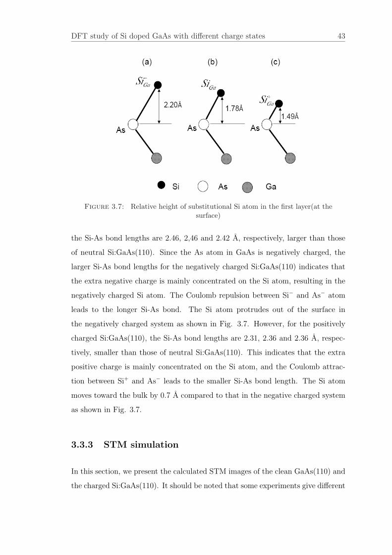
DFT study of Si doped GaAs with different charge states 43
Figure 3.7: Relative height of substitutional Si atom in the first layer(at thesurface)
the Si-As bond lengths are 2.46, 2,46 and 2.42 A, respectively, larger than those
of neutral Si:GaAs(110). Since the As atom in GaAs is negatively charged, the
larger Si-As bond lengths for the negatively charged Si:GaAs(110) indicates that
the extra negative charge is mainly concentrated on the Si atom, resulting in the
negatively charged Si atom. The Coulomb repulsion between Si− and As− atom
leads to the longer Si-As bond. The Si atom protrudes out of the surface in
the negatively charged system as shown in Fig. 3.7. However, for the positively
charged Si:GaAs(110), the Si-As bond lengths are 2.31, 2.36 and 2.36 A, respec-
tively, smaller than those of neutral Si:GaAs(110). This indicates that the extra
positive charge is mainly concentrated on the Si atom, and the Coulomb attrac-
tion between Si+ and As− leads to the smaller Si-As bond length. The Si atom
moves toward the bulk by 0.7 A compared to that in the negative charged system
as shown in Fig. 3.7.
3.3.3 STM simulation
In this section, we present the calculated STM images of the clean GaAs(110) and
the charged Si:GaAs(110). It should be noted that some experiments give different

DFT study of Si doped GaAs with different charge states 44
results since the doping concentration, significantly different tip and the measure-
ment conditions have an important influence on the measured STM images[70].
Fig. 3.8 represents the calculated STM image of the clean neutral GaAs(110)
at bias voltage of 2.0 V. Here the positive bias voltage indicates electrons tunnel
from the probe into the conduction bands. The bright feature of the STM image
corresponds to the large protrusion of the atoms and the dark feature corresponds
to the small protrusion of atoms. The calculated STM image of clean GaAs(110)
in Fig. 3.8 agrees with the experiments [70, 71] and previous theoretical results
[65, 66]. The bright feature corresponds to the empty dangling-bond states of Ga
atoms on the GaAs(110) surface.
The calculated STM images for positively charged donor at bias voltage of 1
V and 2 V are shown in Fig. 3.9 and Fig. 3.10, respectively. The STM image
in Fig. 3.10 is similar to that of the clean GaAs(110), but the Si atom presents
a larger protrusion compared to the Ga atom which is more apparent when the
bias voltate is 1 V shown in Fig. 3.9. The large protrusion of the Si+Ga defect at
the positive bias voltage is similar to the experimental STM image obtained by
Teichmann[72], who pointed out that the extra positive charge of the donor causes
the bands to drop and results in an enhanced tunnel current in the Si atom site.
This overcompensates the reduction of the current from the lower height of Si+Ga(cf.
Fig. 3.7) and corresponding larger distance to the tip. Fig. 3.11 gives the STM
image for the negatively charged system at the bias voltage of 2 V. Different from
the positively charged case, the Si−Ga defect on the surface presents a dark feature.
As discussed in previous section, the extra negative charge is mainly concentrated
on the Si atom for the negatively charged system, and the extra negative charge
occupies the dangling bond of the Si atom. The completely occupied dangling
bond leads to the small protrusion of the negative Si atom at the positive bias
voltage.

DFT study of Si doped GaAs with different charge states 45
Figure 3.8: Calculated STM of clean GaAs(110) at a bias voltage of 2 V forneutral system
Figure 3.9: Calculated STM of Si doped GaAs(110) at a bias voltage of 1 Vfor positively charged Si(charge state: Si+Ga)

DFT study of Si doped GaAs with different charge states 46
Figure 3.10: Calculated STM of Si doped GaAs(110) at a bias voltage of 2V for positively charged Si(charge state: Si+Ga)
Figure 3.11: Calculated STM of Si doped GaAs(110) at a bias voltage of 2V for negatively charged Si(charge state: Si−Ga)

DFT study of Si doped GaAs with different charge states 47
3.4 Conclusions
In this work, firstly, we studied the DX center in bulk GaAs and in GaAs(110).
In bulk GaAs, DX center is found to be a metastable state, in good agreement
with previous calculation of Chadi[51]. However, for surface system, the DX cen-
ter is found to be highly unstable, and the DX formation energy, which depends
on Si position and displacing direction of Si atom in GaAs(110), varies from 0.8
eV to 1.3 eV. Secondly, we found that the extra charge is mainly concentrated
on the defect for charged Si:GaAs(110) where Si atoms replace Ga atoms on the
GaAs(110) surface. On the surface Si−Ga defect is stable, while Si+Ga defect is unsta-
ble. In addition, we also reported the calculated STM images for clean GaAs(110)
and the Si:GaAs(110) with different charge states which agree with experimental
results. We found that the STM image switches from a bright feature to a dark
feature when the charge state of SiGa defect on the surface changes from positive
to negative at the positive bias voltage.

Chapter 4
Many body perturbation theory
4.1 Introduction
So far we have examined how one can justify the reduction of the many-body
equation to a single particle problem. This can be done by introducing certain
approximations. In this Chapter we show that excited-state properties can be
accessed more directly with a purpose built method, the so-called many-body
perturbation theory(MBPT)[10]. The one-particle band-structure paradigm itself
has been deeply revised by the introduction of the concept of quasi-particles, which
provides a proper interpretation of the results of photoemission experiments. Fig.
4.1 gives a schematic illustration. In direct photoelectron spectroscopy a photon
with energy ~ω impinges on the sample and ejects an electron, whose kinetic energy
Ekin is subsequently measured. The binding energy εi of this electron is given by
the difference εi = Ekin− ~ω. In reality, they are correlated through the Coulomb
interaction, and the ejection of an electron is always a many-body process. In this
general sense εi equals the difference εi = EN0 − EN−1
i between the total energy
EN0 of the N particle ground state ΨN
0 and the energy EN−1i of the N − 1 particle
state ΨN−1i that remains after the emission. Inverse photoelectron spectroscopy is
the complementary process: electrons are injected into the sample, and the energy
of the emitted photon is measured. The number of electrons in the system thus
48
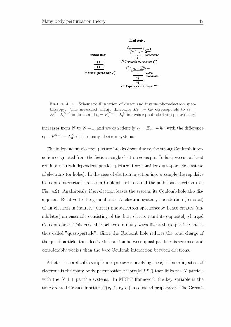
Many body perturbation theory 49
Figure 4.1: Schematic illustation of direct and inverse photoelectron spec-troscopy. The measured energy difference Ekin − ~ω correseponds to εi =EN
0 −EN−1i in direct and εi = EN+1
i −EN0 in inverse photoelectron spectroscopy.
increases from N to N + 1, and we can identify εi = Ekin− ~ω with the difference
εi = EN+1i − EN
0 of the many electron systems.
The independent electron picture breaks down due to the strong Coulomb inter-
action originated from the fictious single electron concepts. In fact, we can at least
retain a nearly-independent particle picture if we consider quasi-particles instead
of electrons (or holes). In the case of electron injection into a sample the repulsive
Coulomb interaction creates a Coulomb hole around the additional electron (see
Fig. 4.2). Analogously, if an electron leaves the system, its Coulomb hole also dis-
appears. Relative to the ground-state N electron system, the addition (removal)
of an electron in indirect (direct) photoelectron spectroscopy hence creates (an-
nihilates) an ensemble consisting of the bare electron and its oppositely charged
Coulomb hole. This ensemble behaves in many ways like a single-particle and is
thus called ”quasi-particle”. Since the Coulomb hole reduces the total charge of
the quasi-particle, the effective interaction between quasi-particles is screened and
considerably weaker than the bare Coulomb interaction between electrons.
A better theoretical description of processes involving the ejection or injection of
electrons is the many body perturbation theory(MBPT) that links the N particle
with the N ± 1 particle systems. In MBPT framework the key variable is the
time ordered Green’s function G(r1, t1, r2, t2), also called propagator. The Green’s

Many body perturbation theory 50
Figure 4.2: The coulomb hole around an electron together with the bareelectron forms the quasi-particle, as can be seen from the figure in the right.Quasi-particles interact via a weak screened interaction W instead of the strong
coulomb interaction v(see the figure in the left).
function contains the excitation energies and excitation lifetimes. Besides, we
can directly obtain the ground-state electron density, the expectation values of
one-particle operators and the ground-state total energy from it. The Green’s
function is hence capable of giving access to the same observables as the ground-
state electron density. In contrast to the DFT expression E(ρ), the functional
E(G) is even known exactly[73]. While the Green’s function contains much more
information than the electron density, it is also a more complicated function and
thus rarely applied to ground-state properties.
4.2 The Green’s function
In this section we introduce the time-ordered Green’s function and examine its
properties. The Green’s function describes the probability amplitude for the prop-
agation of an electron(hole) from position r1 at time t1 to the position r2 at time
t2. For the propagation of an additional electron from (r2, t2) to (r1, t1) in a many
electron system, the time-ordered one-particle Green’s function at zero tempera-
ture is defined as:
Ge(1, 2) = − i
~〈N, 0|ψ(1)ψ+(2)|N, 0〉θ(t1 − t2) (4.1)
where 〈N | is the exact ground state of the interacting system. The ψ and ψ+ oper-
ators are annihilation and creation field operators within Heisenberg picture(they

Many body perturbation theory 51
contain the whole time dependence), respectively. Index 1 is shorthand for posi-
tion, time and spin variables(r1, t1, σ1). θ(t1 − t2) is the Heaviside step function
defined by
θ(t1 − t2) =
1, t1 > t2
0, t1 < t2(4.2)
Similarly, we have the green’s function
Gh(2, 1) = − i
~〈N, 0|ψ+(2)ψ(1)|N, 0〉θ(t2 − t1) (4.3)
for the propagation of an additonal hole from (r1, t1) to (r2, t2). For convenience,
we combine the two expressions in one time-ordered Green’s function
G(1, 2) = Ge(1, 2)−Gh(2, 1) = − i
~〈N, 0|T [ψ(1)ψ+(2)]|N, 0〉
=
− i~〈N, 0|ψ(1)ψ+(2)|N, 0〉, t1 > t2
i~〈N, 0|ψ+(2)ψ(1)|N, 0〉, t1 < t2
(4.4)
where T stands for the Wick time-ordering operator, which has the effect of or-
dering the operator with largest time on the left. The physically intuitive inter-
pretation of the time-ordered Green’s function can be emphasized from Eqs.(4.4).
When t1 is larger than t2, the Green’s function describes the probability to find an
electron in r1 with spin σ1 at time t1, when an electron was added in r2 with spin
σ2 at time t2 to the system in its ground-state. Instead, when t1 is smaller than
t2, the Green’s function describes the probability to find a hole in r2 with spin σ2
at time t2, when an electron was previously removed in r1 with spin σ1 at time t1.
The one-particle Green’s function G contains a great deal of useful information.
According to G, we can calculate also the ground-state expectation value of any
one-particle operator and the ground-state energy of the system. For example,
the expectation value of electron denstiy ρ(r, t) can be expressed in terms of the
Green’s function as
ρ(r, t) = 〈N, 0|φ+(r, t)φ(r, t)|N, 0〉 = −i~G(r, t, r, t+ η) (4.5)

Many body perturbation theory 52
Here η is an infinitesimal positive number. It serves only to enforce the correct
order of the field operators. Its unit should always be clear from the context;
presently it is an infinitesimally small time.
Similarly, the Galitskii-Migdal formula[74] gives the ground-state total energy
as a function of the one-particle Green’s function only:
E = −i~2
∑σ1,σ2
δσ1,σ2
∫dr1 lim
r2→r1
limt2→t+1
[i∂
∂t1+ h0(r1)]G(1, 2) (4.6)
where h0 = −∇22 + vext is the one particle Hamitonian. The one-particle exci-
tation spectrum carried by the Green’s function will be made obvious in the next
section.
4.3 Lehmann representation
For convenience, I will employ atomic units(i.e. ~ = 1) in the next part. The so-
called Lehmann representation of the Green’s function permits one to get insight
into its physical meaning. It shows that the Green’s function is closely related
to the single-particle excitation energies of the system. If we insert the closure
relation∑
i |N ± 1, i〉〈N ± 1, i| = 1 between the two field operators in Eqs. (4.4),
where |N±1, i〉 is the complete set of state vectors of the N±1 particle system,
then the Green’s function depends only on the difference τ = t1− t2 in the case of
time-independent Hamitonian:
iG(r1, r2, τ) = θ(τ)∑
i
〈N, 0|ψ(1)|N + 1, i〉〈N + 1, i|ψ+(2)|N, 0〉
− θ(−τ)∑
i
〈N, 0|ψ+(2)|N − 1, i〉〈N − 1, i|ψ(1)|N, 0〉 (4.7)
In the above equation, if τ > 0, only states with N + 1 survive; if τ < 0, only
states with N − 1 survive. The index i sums over all states of a given particle
number.

Many body perturbation theory 53
For positive time (τ > 0),the excitation energy of a system previously in its
ground-state that, due to an additional electron, is now in the excited state i of
N + 1, is given by
εN+1i = EN+1,i − EN,0 (4.8)
Similarly, for negative time τ < 0, a hole energy in its excited state is given by
εN−1i = EN,0 − EN−1,i (4.9)
The time dependence of the matrix elements can be handled by introducing the
Schrodinger picture:
ψH(r1, t1) = eiλt1ψS(r1)e−iλt1 (4.10)
where λ corresponds to the excitation energy. ψH(r1, t1) is field operator in the
Heisenberg picture. ψS(r1) is the field operator in the Schrodinger picture. There-
fore, the Green’s function takes the following form
iG(r1, r2, τ) = θ(τ)∑
i
〈N, 0|ψS|N + 1, i〉〈N + 1, i|ψ+S (2)|N, 0〉e−iεN+1
i τ
− θ(−τ)∑
i
〈N, 0|ψ+S (2)|N − 1, i〉〈N − 1, i|ψS(1)|N, 0〉e−iεN−1
i τ(4.11)
The minimum energy of the lowest conduction state is given by
εc = EN+1,0 − EN,0 (4.12)
Alternatively, the minimum energy of the highest valence state, which is required
to remove an electron is given by
εv = EN,0 − EN−1,0 (4.13)
If the system is semiconductor or insulator, the band gap Eg is defined as the
energy difference between the conduction and valence states
Eg = εc − εv = EN+1,0 + EN−1,0 − 2EN,0 (4.14)

Many body perturbation theory 54
If the system is metallic system, the energy εc = εv is the chemical potential µ. For
semiconductor or insulator system, the chemical potential µ lies somewhere inside
the gap. Therefore, if εi > µ, the energy is defined as EN+1,i − EN , if if εi < µ,
the energy is given by EN − EN−1,i. Consequently, we can define the so-called
Lehmann amplitudes fi(r),
fi(r) =
〈N, 0|ψS(r)|N + 1, i〉, εi > µ
〈N − 1, i|ψS(r)|N, 0〉, εi < µ(4.15)
The Green’s function is then expressed as
iG(r1, r2, τ) =∑
i
[θ(τ)θ(εi − µ)− θ(−τ)θ(µ− εi)]fi(r1)f∗i (r2)e
−iεiτ (4.16)
Now the sum∑
i is over electron and hole states. Fourier transformation of Eqs.
(4.16) to the frequency axis using the Fourier transform of the Heaviside step
function
θ(±τ) = ∓ 1
2πi
∫ ∞
−∞
e−iωτ
ω ± iηdω (4.17)
for η → 0+, one obtains the Lehmann representation of one particle Green’s func-
tion
G(r1, r2, ω) =∑
i
fi(r1)f∗i (r2)
ω − εi + iηsign(εi − µ)(4.18)
The Green’s function has poles at the true many particle excitation energies εN±1i .
The poles lie slightly above the real axis for frequencies below µ and slightly below
the real axis for frequencies above µ, as shown in Fig. 4.3.
It must be emphasised that the concept of a quasi-particle is an interpretation
of the experimentally observed many body spectrum in terms of one-particle-like
excitations. The quasi-particle concept is used for various types of excitations, for
instance electron-hole pairs (excitons) or vibrations (phonons). In the context of
one-electron excitations, these quasiparticles can be viewed as a hole or an electron
surrounded by its polarisation cloud. Quasi-particles have a finite lifetime due
to dephasing, i.e., decay into other quasi-particles, because the true many-body

Many body perturbation theory 55
Figure 4.3: In the complex plane, the Green’s function has poles(crosses) onlyalong the real axis. The poles are located above the real axis for frenquencieslower than the chemical potential µ, and below for frequencies greater than µ
eigenstates may contribute to more than one quasi-particle. In other words, a
quasi-particle is not an eigenstate of the system but a superposition of eigenstates.
4.4 Spectral function
We apply the following relation
limη→0+
1
x+ iη= ℘
1
x− iπδ(x) (4.19)
to the Eqs.(4.18), where ℘ 1x
is the principal value of 1x, one can obtain the imagi-
nary part of G:
ImG(r1, r2, ω) = πsign(µ− εi)∑
i
fi(r1)f∗i (r2)δ(ω − εi) (4.20)
The spectral function is defined as
A(r1, r2, ω) =1
πsign(ω − µ)ImG(r1, r2, ω) =
∑i
fi(r1)f∗i (r2)δ(ω − εi) (4.21)

Many body perturbation theory 56
The spectral function A is a positive function of ω. From this expression one
can immediately realize that the spectral function is hence the quantity directly
related to the one-particle excitations, described by the Lehmann amplitudes fi
and the electron addition and removal energies εi. Moreover, the spectral function
allows us to rewrite the Eqs. (4.18) as an integral over frequencies
G(r, r′, ω) =
∫ µ
−∞
A(r, r′, ω)
ω − ω′ − iηdω′ +
∫ ∞
µ
A(r, r′, ω)
ω − ω′ + iηdω′ (4.22)
Since
∑i
fi(r1)f∗i (r2) =
∑i
〈N |ψ+(2)|N − 1, i〉〈N − 1, i|ψ(r1)|N〉
+∑
i
〈N |ψ(r1)|N + 1, i〉〈N + 1, i|ψ+(r2)|N〉
= 〈N |[ψ(r1), ψ+(r2)]+|N〉
= δ(r1 − r2) (4.23)
The spectral function satisfies the normalization condition:
∫ ∞
−∞A(r1, r2, ω)dω = δ(r1 − r2) (4.24)
and from its diagonal one can extract important information such as the electronic
density:
ρ(r) =
∫ µ
−∞A(r, r, ω)dω (4.25)
Since the connection between Green’s function and spectral function has been
demonstrated, now I will show how to calculate the spectra of photoemission ex-
periments. In a photoemission experiment, the detector measures electrons that
are extracted from a solid due to an incident photon, and the experimental ob-
servable in PES is the photocurrent. It is given by
I ∼∫dr1
∫dr2φ
∗pe(r1)δH(r1)A(r1, r2, E)δH(r2)φpe(r2) (4.26)

Many body perturbation theory 57
where r comprises a spatial and a spin coordinate. φpe is a is a time-reversed
damped LEED state describing the photoelectron that reaches the detector. δH(r)
is the perturbing field that excites the electron. Inserting Eqs.(4.25) into Eqs.(4.26)
we obtain Fermis golden rule expression
I ∼∑
i
|〈φpe|δH|fi〉|2δ(E − εi) (4.27)
The magnitude of the transition matrix elements can vary considerably between
different states and even become zero, in particular when the symmetry of the
system defines selection rules. The photocurrent therefore reflects only a somewhat
distorted picture of the electron density of states (DOS)
N el(E) =∑
i
δ(E − εi) =
∫d3rA(r, r, E) (4.28)
4.5 Hedin’s equations and the GW approxima-
tion
With the equation of motion for the Heisenberg creation and annihilation field
operators ψ and ψ+(see Appendix(A.1)), the one-particle Green’s function depends
on the two particle Green’s function, and is given by
[i∂
∂t1− h0(1)]G(1, 2) = δ(1, 2)− i
∫d3v(1, 3)G2(1, 3, 2, 3
+) (4.29)
where h0 = −∇2
2+Vext is the one-particle term of the Hamitonian. The two-particle
Green’s function G2 describes the creation and annihilation of pairs of particles.
Further deriving the equation of motion for G2, one would obtain higher orders
of Green’s function G2, G3 · · · . The physical meaning of this is that the electron
hole pair created by the propagation of the first electron would induce a cascade
of other electron-hole pairs. Therefore, the system of equations will become more
and more complex with the increase of higher order Green’s function. In fact, if
one only needs to know the one particle Green’s function, a good approximation,

Many body perturbation theory 58
which allows one to express the two particle Green’s function in terms of one-
particle ones, can be introduced. Similarly, if somebody want to calculate the
absorption spectra(involving two-particle Green’s function), one needs to find an
approximation to replace the three-paritcle Green’s function with the two-particle
ones. This is the fundamental idea of many body perturbation theory, which
provides a scheme to systematically find approximations for the higher-number of
particle Green’s functions in terms of the lower ones.
In this thesis, I am interested in the one particle Green’s function. Within the
idea of many body perturbation theory(MBPT), it allows one to get rid of the
two particle Green’s function in the Eqs.(4.29), while retaining only the terms
dependent on one-particle Green’s functions. This is achieved by introducing the
Schwinger derivative technique[75]. The main physical idea of Schwinger is that
the same polarization of the system could be obtained by a small time-dependent
perturbing external potential Uper(1, 2), which, in the spirit of the linear-response
theory, will be made vanish at the end of the derivation. The following expansion
presents the variation of G with respect to perturbation Uper(See Appendix(A.2)
for detailed information):
δG(1, 2)
δUper(3)= G(1, 2)G(3, 3+)−G2(1, 3, 2, 3
+) (4.30)
Hence the two particle Green’s function is expressed as terms of one particle
Green’s function by introducing the variation of G with respect to perturbation
Uper. Inserting above equation in Eqs.(4.29), we can obtain:
[i∂
∂t1− h0(1) + i
∫d3v(1, 3)G(3, 3+)]G(1, 2)− i
∫d3v(1, 3)
δG(1, 2)
δUper(3)= δ(1, 2)
(4.31)
In the above equations G(3, 3+) is the electronic denstiy ρ(3), so the Hartree
potential VH(1) is described by the term −i ∫ d3v(1, 3)G(3, 3+). The self energy
is defined by the last term of Eqs.(4.31)
i
∫d3v(1, 3)
δG(1, 2)
δUper(3)=
∫d3Σ(1, 3)G(3, 2) (4.32)

Many body perturbation theory 59
The self energy describes all the effects of exchange and correlation in the system(
i.e. all the interacting effects are includes in the self energy Σ). With the intro-
duction of the Hartree potential VH and the self energy Σ, Eqs.(4.31) can be then
rewritten as:
[i∂
∂t1− h0(1)− VH(1)]G(1, 2) = δ(1, 2) +
∫d3Σ(1, 3)G(3, 2) (4.33)
The above equation is the so-called Dyson equation. The equation of motion of
the non-interacting Green’s function G0 is given by
[i∂
∂t1− h0(1)− VH(1)]G0(1, 2) = δ(1, 2) (4.34)
The above equation shows that non-interacting Green’s function is formally the
functional inverse of the operator (ω− h0 − VH(1)) in frequency space. So we can
rewrite the Dyson Eqs.(4.33) as
G(1, 2) = G0(1, 2) +
∫d34G0(1, 3)Σ(1, 3)G(4, 2) (4.35)
In order to evaluate the self energy, by introducing∫d5G−1(4, 5)G(5, 2) = δ(4, 2),
the Eqs.(4.33) can be rewritten as
[i∂
∂t1−h0(1)−VH(1)]G(1, 2)−i
∫d345v(1+, 3)
δG(1, 4)
δUper(3)G−1(5, 2) = δ(1, 2) (4.36)
Inserting the relation
δF (1, 2)
δG(3)= −
∫d45F (1, 4)
δF−1(4, 5)
δG(3)(4.37)
to the last term in the left-hand-side of Eqs.(4.36), yields the self energy operator
as
Σ(1, 2) = −i∫d34v(1+, 3)G(1, 4)
δG−1(4, 2)
δUper(3)(4.38)
Now let us insert the chain rule
δF [G[H]](1)
δH(2)=
∫d3δF [G](1)
δG(3)
δG[H](3)
δH(2)(4.39)

Many body perturbation theory 60
via V in the definition of self energy of Eqs.(4.38):
Σ(1, 2) = −i∫d345v(1+, 3)G(4, 2)
δG−1(1, 4)δV (5)
δUper(3)δV (5)(4.40)
where V is the local classical potential, and defined as the sum of the external
perturbation and the Hartree potential:
V (1) = U(1)− i
∫d2v(1, 2)G(2, 2+) (4.41)
With the introdcution of the irreducible vertex Γ
Γ(1, 2, 3) = −G−1(1, 2)
δV (3)(4.42)
and the definition of time ordered inverse dielectric function:
ε−1(1, 2) =δV (1)
δU(2)(4.43)
In addition, one can introduce W , the dynamical screened Coulomb interaction,
and defined by
W (1, 2) =
∫d3v(1, 3)ε−1(3, 2) (4.44)
Finally, the self energy is expressed as
Σ(1, 2) = i
∫d34G(1, 4)W (3, 1+)Γ(4, 2, 3) (4.45)
Now let us further evaluate Γ, using Dyson equation G−1 = G−10 − V − Σ, Γ is
easily obtained:
Γ(1, 2, 3) = δ(1, 2)δ(1, 3) +δΣ(1, 2)
δV (3)
= δ(1, 2)δ(1, 3) +
∫d45
δΣ(1, 2)G(4, 5)
G(4, 5)δV (3)
= δ(1, 2)δ(1, 3) +
∫d4567
δΣ(1, 2)
δG(4, 5)
× G(4, 6)G(7, 5)Γ(6, 7, 3) (4.46)
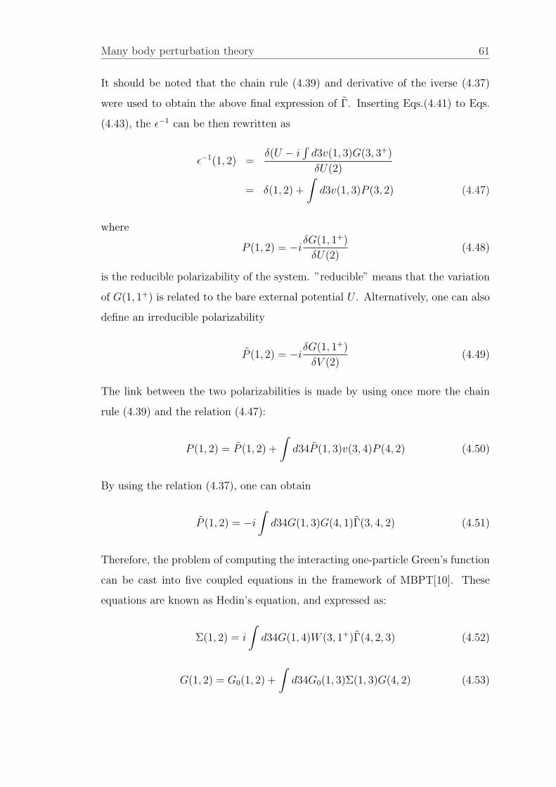
Many body perturbation theory 61
It should be noted that the chain rule (4.39) and derivative of the iverse (4.37)
were used to obtain the above final expression of Γ. Inserting Eqs.(4.41) to Eqs.
(4.43), the ε−1 can be then rewritten as
ε−1(1, 2) =δ(U − i
∫d3v(1, 3)G(3, 3+)
δU(2)
= δ(1, 2) +
∫d3v(1, 3)P (3, 2) (4.47)
where
P (1, 2) = −iδG(1, 1+)
δU(2)(4.48)
is the reducible polarizability of the system. ”reducible” means that the variation
of G(1, 1+) is related to the bare external potential U . Alternatively, one can also
define an irreducible polarizability
P (1, 2) = −iδG(1, 1+)
δV (2)(4.49)
The link between the two polarizabilities is made by using once more the chain
rule (4.39) and the relation (4.47):
P (1, 2) = P (1, 2) +
∫d34P (1, 3)v(3, 4)P (4, 2) (4.50)
By using the relation (4.37), one can obtain
P (1, 2) = −i∫d34G(1, 3)G(4, 1)Γ(3, 4, 2) (4.51)
Therefore, the problem of computing the interacting one-particle Green’s function
can be cast into five coupled equations in the framework of MBPT[10]. These
equations are known as Hedin’s equation, and expressed as:
Σ(1, 2) = i
∫d34G(1, 4)W (3, 1+)Γ(4, 2, 3) (4.52)
G(1, 2) = G0(1, 2) +
∫d34G0(1, 3)Σ(1, 3)G(4, 2) (4.53)

Many body perturbation theory 62
P (1, 2) = −i∫d34G(1, 3)G(4, 1)Γ(3, 4, 2) (4.54)
W (1, 2) = v(1, 2) +
∫d3d4v(1, 3)P (3, 4)W (4, 2) (4.55)
Γ(1, 2, 3) = δ(1, 2)δ(1, 3) +
∫d4567
δΣ(1, 2)
δG(4, 5)
× G(4, 6)G(7, 5)Γ(6, 7, 3) (4.56)
These equations involve the independent particle and full Green’s function G0
and G, the polarisation P , the bare and screened interaction v and W , the self-
energy Σ, and the so-called vertex function Γ. For simplicity, we use the notation
1 = (r1, t1, σ1) for every pair of one spatial and one temporal variable. 1+ indicates
that the time argument has been increased by an infinitesimally small, positive
amount.
Hedin’s scheme provides directly a set of equations in terms of G and W and
in particular an expansion of Σ in terms of W . Expansions in terms of v are
known to fail: for instance, the second order term in v for the correlation energy
of an homogenous electron gas is infinite[76]. The idea of using an interaction,
namely W , weaker than v as coupling constant of the perturbative expansion
was already introduced by Hubbard[77]. The screened Coulomb interaction is
intuitively smaller than the bare one, as the interaction between two electrons
being part of a system is reduced by the dielectric constant of the medium or, in
other words, by the screening due to all the other electrons of the system.
This set of coupled equations cannot be solved directly due to the presence
of the functional derivative in the definition of the vertex function. However,
it is amenable to physically meaningful approximations. We will describe the
equations in more detail before coming to the most important approximation, the
GW approximation.
Eqs.(4.53) and Eqs.(4.55) have the same structure, known as Dyson equation. Σ
represents the complicated correlation effects of a many particle system. G0 and G
correspond to the propagation of electrons or holes in the system, whereas v andW

Many body perturbation theory 63
can be interpreted as propagators for the quantum particles of the electric field.
Thus, the polarisation function plays the role of the self-energy for the electric
field particles, changing the bare Coulomb interaction into the screened Coulomb
interaction.
Correspondingly, Eqs.(4.52) and Eqs.(4.54) have the same structure. They con-
tain two propagators connected to one point of the interaction kernel and are
connected via the vertex function to the other point of the kernel. This vertex
function is a three-point kernel that describes all possible ways how a (dressed)
electron is scattered when a (screened) electric field particle is created or annihi-
lated.
When a charge is added to an electronic system, the first effect is the polar-
ization of the system. By neglecting the electron-hole interaction(short range
effect) in the electron-hole pairs that constitute the polarization and the exchange
correlation effects in the induced interaction between the extra charge and the
polarization charge of the system,(i.e. approximating the vertex function by its
first term: Γ(1, 2, 3) = δ(1, 2)δ(2, 3)) one finds the GW approximation introduced
by Hedin[11]
Σ(1, 2) = iG(1, 2)W (1+, 2) (4.57)
The GW approximation corresponds to neglecting vertex effects, i.e. to taking for
the vertex the simplest expression:
Γ(1, 2, 3) = δ(1, 2)δ(2, 3) (4.58)
Similarly, If one neglects the vertex effects in the polarization P , the random-phase
approximation(RPA) for P is obtained:
P (1, 2) = −iG(1, 2)G(2, 1) (4.59)
Even using the GW approximation to the self-energy, the Dyson equation is still
a self-consistent equation in G that one could solve iteratively. However, this
is rarely done. Instead of using the full Green’s function G, the non-interacting

Many body perturbation theory 64
Green’s function G0 is used as a first approximation in Eqs.(4.57) and Eqs.(4.59).
We use this approach, denoted as G0W0 in all the actual calculations.
4.6 Quasi-particle equations
In reality, the quasi-particle quantities are not calulated from the Dyson Eqs.(4.33).
Let us reformulate the Dyson Eqs.(4.33). The Fourier transform of the Dyson
Eqs.(4.33) gives:
[ω − h0(1)− VH(1)]G(1, 2, ω)−∫d3Σ(1, 3, ω)G(3, 2, ω) = δ(1, 2) (4.60)
A pratical solution of this equation is obtained by using a the biorthonormal
representation[78],
G(r1, r2, ω) =∑
λ
φλ(r1, ω)φ∗λ(r2, ω)
ω − Eλ(ω)(4.61)
with φλ(r1, ω) and φ∗λ(r2, ω) being solutions of
[h0(r1) + VH(r1)]φλ(r1, ω) +
∫dr2Σ(r1, r2, ω)φλ(r2, ω) = Eλ(ω)φλ(r1, ω) (4.62)
and
[h0(r1) + VH(r1)]φ∗λ(r1, ω) +
∫dr2Σ
′(r1, r2, ω)φ∗λ(r2, ω) = E∗λ(ω)φ∗λ(r1, ω) (4.63)
where Σ′(r1, r2, ω) = [Σ(r2, r1, ω)]∗. In the Lehmann representation in the ther-
modynamic limit one has a series of infinite close-lying poles on the real axis that
merge to form a branch-cut. An alternative representation is given by a com-
plex pole(i.e. the quasi-particle energy). A schematic comparison between the
Lehmann representation and quasi-particle pole representation is given in Fig.4.4.
The quasi-particle concept is based on the assumption that the full energy de-
pendence of G(r1, r2, ω) can be described approximately with some well defined

Many body perturbation theory 65
Figure 4.4: Schematic comparison for the Lehmann representation(left) andthe quasi-particle pole representation(right). A series of close lying poles onthe real axis in the Lehmann representation can be equivalently represented bya single pole in the complex plane. The real part of the pole corresponds tothe the position of the peak, which represents the quasi-particle energies. Theimaginary part of pole in the complex plane gives the width of peak, which is
connected to the lifetime of excitation [79].
complex poles
G(r1, r2, ω) ≈∑
λ
φλ(r1, εQPλ )φ∗λ(r2, ε
QPλ )
ω − εQPλ
(4.64)
with the quasi-particle energies defined by
εQPs = Eλ(ε
QPs ) (4.65)
In this way, one finds the quasi-particle equation:
[h0(r1) + VH(r1)]φs(r1) +
∫dr2Σ(r1, r2, E
QPs )φs(r2) = Esφs(r1) (4.66)
Strictly speaking, this equation has, in general, no real-valued solutions, because
the nonlocal, frequency dependent potential Σ is, in general, not hermitian.

Chapter 5
Quasi-particle bandstructures and
lifetimes in metallic systems
5.1 Introduction
In the last decade the electronic band structures and electron scattering in noble
metals have been studied using experimental techniques[8, 80, 81] and a variety
of theoretical methods [13, 14, 82, 83]. The GW approximation derived by Hedin
in 1965 [11] has become the state-of-the-art approach to study the quasi-particle
band-structures and lifetimes [13, 14, 82, 83] of a large number of systems going
beyond the well-known Density Functional Theory(DFT).
It is well known that the usual local density approximation (LDA) [3] under-
estimates the band gaps for the semiconductors, which can be improved by using
the so-called scissors operator(i.e. by rigidly shifting the conduction bands to
higher energy). However, for the noble metals the quasiparticle corrections are
both k-point and band dependent [13], so a scissors operator is useless. Another
important drawback of the traditional DFT is that the exchange-correlation part
is real, and hence infinit lifetime, whereas the lifetime of excited electrons and
holes in metals is known to be finite.
66

Quasi-particle bandstructures and lifetimes in metallic systems 67
A significant numerical problem when performing GW calculations for noble
metals is given by the issue of basis set expansion. The presence of strongly
localized d bands and the inclusion of semicore states for Cu and Ag make the
Ab-initio calculations based on a plane wave expansion basis much heavier than
those for semiconductors. For the case of Cu, plane waves with cutoff energy
of at least 160 Ry (about 2700 plane waves) are needed for convergence [13].
GW calculations need larger computational requirements than DFT, in particular
for the calculations of surfaces and bulk solids with occupied d orbitals [84]. It
turned out that a Gaussian-orbital basis set instead of using plane-wave Fourier
representations of the relevant two-point functions is efficient for the evaluation of
GW self-energy corrections [84]. Another common simplification, i.e. the Plasmon-
pole approximation(RPA) of the frequency dependence of ε(ω) should be avoided
for the GW calculation of Cu [13], which means that the dielectric matrix ε−1GG′(q;ω)
should be computed explicitly by performing the energy integral numerically. This
imposes further heavy CPU load for the GW calculation with plane waves.
Most previous lifetime calculations are based on the DFT band energies [24, 25,
26, 27, 82]. Furthermore, the so-called ’energy shell’ approximation with renor-
malization factor equal to unity was employed to obtain the imaginary part of
the quasi-particle energies. In fact, the renormalization factor for noble metals
varies between 0.57 and 0.77 [83]. The renormalization factor directly changes the
quasiparticle energies, and also changes the quasiparticle lifetimes. Because of the
large discrepancies between DFT band energies and experiments, the calculated
lifetimes based on the DFT energies are not consistent with experiment. In order
to compare the calculated lifetimes based on the DFT band energies with exper-
iments, the DFT band energies have to be shifted rigidly(which, as mentioned
above, is questionable in metals).
So far the quantitative understanding of excitation mechanisms and their re-
laxation channels is far from being complete. In many cases the GW approach
correctly reproduces the changes of experimental electron relaxation times with
the excitation energy [87]. However, large discrepancies between theoretical and
experimental results occur for d holes in Cu and Ag. The lifetimes of holes at
Quasi-particle bandstructures and lifetimes in metallic systems 68
the top of d bands as calculated in Ref. [82, 83] appear to be almost twice longer
than the experimentally derived lifetimes. Ref. [86] argued that due to the shifted
d bands in the DFT calculation the available phase space for Auger recombina-
tion is underestimated yielding calculated lifetimes which are too long. However,
Ref. [83, 87] conclude that the drawbacks of the LDA band structures do not lead
to qualitative changes of the quasiparticle lifetimes. The quasiparticle lifetime cal-
culations based on the exact band energies have been performed for Cu using plane
waves method [85]. However, because of large requirements of the computation,
only several lifetimes at high symmetry points were calculated. Ref. [83] calculate
the lifetimes based on the corrected local density approximation, but the d band
threshold energies (1.7 eV for Cu, 3.2 eV for Ag) reported in this thesis are still
close to the Fermi level, compared to the photoemission data about 2 eV for Cu
and about 3.8 eV for Ag. So it is necessary to calculate the lifetimes based on the
accurate quasiparticle band energies.
In this chapter we go beyond the ’energy shell’ approximation to calculate the
lifetimes of electrons and holes for Cu and Ag based on the accurate GW band-
structure energies, using the efficient localized Gaussian orbitals. Firstly, we dis-
cuss the quasiparticle bandstructures for Cu and Ag. Then we analyze the influ-
ence of the quasiparticle corrections to the lifetimes. Our calculation starts with a
DFT calculation of the ground-state properties performed using norm-conserving
pseudopotentials, then the calculated DFT band structure energies and wave func-
tions are used within the GW approximation framework for the calculation of the
self energy operator, whose real part yields the quasi-particle band energies and
imaginary part yields the lifetimes.
A particular field of research is given by the lifetimes of metal surface states ,
which can be drastically different from the lifetimes of bulk states. Unfortunately,
the calculation of the GW self-energy operator of a surface system(e.g. in a slab
configuration) would be very time-consuming [88] and has been carried out so
far only for the relatively simple Be(001) suface [89]. So far, The most previous
works calculate image state lifetimes for the more complex noble-metal surfaces by
employing a realistic one-dimensional model potential [90] instead of the full three

Quasi-particle bandstructures and lifetimes in metallic systems 69
dimensional pseudopotential. Within this simple model, the surface corrugation
is fully neglected(i.e. a single electron moving in an effective potential V(z) is
translationally invariant in the plane of the surface). Here, we report a full three-
dimensional calculation for the image states lifetimes of Cu(100) by using the
efficient localized Gaussian basis sets. With my knowledge, this is the first time
for the evaluation of the image states of noble metal surfaces by performing a full
three-dimensional caculation.
One particular aim of our work is to provide an approach to both band-structure
energies and their lifetimes within one calculation within the GW approximation
for the self energy. For computational purposes many calculations so far have
focused on either the band structure (which can often be obtained within the
plasmon-pole approximation of the GWA, leading to a real self energy and thus
infinite lifetime) or on the lifetime (which can be done efficiently by considering a
limited number of bands in the calculation). Here we show that both quantities
are in fact obtained when the complex nature of the dielectric screening and the
self energy are treated carefully.
This chapter is organized as follows. In Sec. 5.2, we discuss some details of
the GWA and summarize the basic equations needed for the following discussions.
In Sec. 5.3, we discuss the quasi-particle bandstructures for bulk Cu and Ag.
In Sec. 5.4, we present the quasi-particle lifetimes for Cu and Ag based on the
accurate quasiparticle energies. In Sec. 5.5, a full three-dimensional calculation
for the image potential state lifetimes of Cu(100) is reported. A short summary
concludes this chapter in Sec. 5.6.

Quasi-particle bandstructures and lifetimes in metallic systems 70
5.2 Computational details and theoretical meth-
ods
The starting point of the calculation of band structures and lifetimes is given by
a DFT calculation (referring to the electronic ground state), in which the Kohn-
Sham equation
− ~
2
2m∇2 + VPS(r) + VH(r) + VXC(r))
Ψnk(r) = EnkΨnk(r) (5.1)
is solved.
In here, VPS and VH are the ions and Hartree potential, respectively. Since
the d electrons have to be considered as valence electrons, the entire shell to
which they belong must be included as valence states throughout the calculations
[13, 91]. For Ag we employ a norm-conserving pseudopotentia1 constructed along
Hamann’s scheme [38], based on the ionic configuration 4s24p64d10. For Cu, on the
other hand, the transferability of such a pseudopotential seems not guaranteed.
Therefore we employ a multireference pseudopotential (MRPP) constructed along
Carlos’ scheme [92], based on the configuration 3s23p63d104s1. Gaussian orbitals
are used to construct the LDA basis sets. We use 50 Gaussian orbitals of s, p, d
and s* type for Cu atom and 60 Gaussian orbitals of s, p, d and s* type for Ag
atom. The decay constants are 0.18, 0.50, 1.24, 3.2 and 8.5 for Cu, and 0.16, 0.50,
1.40, 3.00, 6.5 and 14.0 for Ag, respectively.
Based on the DFT results, the final treatment of band structures and lifetimes
is done within many body perturbation theory (MBPT) [10]. Assuming that the
electronic spectrum is still given by well-defined quasi particles, excited holes and
electrons are described by an equation of motion
− ~
2
2m∇2 + VPS(r) + VH(r)
ΨQP
nk (r)
+
∫Σ(r, r′, EQP
nk )ΦQPnk (r′)d3r′ = EQP
nk ΨQPnk (r) (5.2)
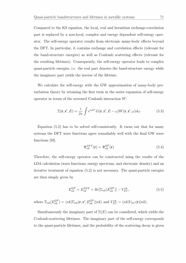
Quasi-particle bandstructures and lifetimes in metallic systems 71
Compared to the KS equation, the local, real and hermitian exchange-correlation
part is replaced by a non-local, complex and energy dependent self-energy oper-
ator. The self-energy operator results from electronic many-body effects beyond
the DFT. In particular, it contains exchange and correlation effects (relevant for
the band-structure energies) as well as Coulomb scattering effects (relevant for
the resulting lifetimes). Consequently, the self-energy operator leads to complex
quasi-particle energies, i.e. the real part denotes the band-structure energy while
the imaginary part yields the inverse of the lifetime.
We calculate the self-energy with the GW approximation of many-body per-
turbation theory by retaining the first term in the series expansion of self-energy
operator in terms of the screened Coulomb interaction W :
Σ(r, r′, E) =i
2π
∫eiω0+
G(r, r′, E − ω)W (r, r′, ω)dω (5.3)
Equation (5.2) has to be solved self-consistently. It turns out that for many
systems the DFT wave functions agree remarkably well with the final GW wave
functions [93].
ΨDFTnk (r) = ΨQP
nk (r) (5.4)
Therefore, the self-energy operator can be constructed using the results of the
LDA calculation (wave functions, energy spectrum, and electronic density) and an
iterative treatment of equation (5.2) is not necessary. The quasi-particle energies
are then simply given by
EQPnk = EDFT
nk +Re[Σnk(EQPnk )]− V nk
XC , (5.5)
where Σnk(EQPnk ) = 〈nk|Σnk(r, r
′, EQPnk )|nk〉 and V nk
XC = 〈nk|VXC(r)|nk〉.
Simultaneously the imaginary part of Σ(E) can be considered, which yields the
Coulomb-scattering lifetimes. The imaginary part of the self-energy corresponds
to the quasi-particle lifetimes, and the probability of the scattering decay is given

Quasi-particle bandstructures and lifetimes in metallic systems 72
by
τ−1nk = 2|Im[Σnk(E
QPnk )]| (5.6)
The numerical evaluation of the GW self-energy operator for the present case
of metals, aiming at its real part and its imaginary part on equal footing, is more
demanding than the common techniques for GW calculations which focus on the
band structure alone, and is also more demanding than the evaluation of lifetimes
alone.
One key quantity is given by the time-ordered polarizability of the system,
P = −iGG, which we calculate from DFT-LDA quantities. For a periodic system
it can be represented by basis functions χβ(q, r), leading to a matrix representation
Pββ′(q, ω) = 21
V
∑
k
∑m
∑n
Mmnβ (k,q)
[Mmn
β′ (k,q)]∗
Θ(EF − Emk)Θ(En,k+q − EF )
×[
1
Emk − En,k+q − ω + i0++
1
Emk − En,k+q + ω + i0+
](5.7)
with spatial integrals Mmnβ (k,q) =
∫ψ∗mk(r)χ
∗β(q, r)ψn,k+q(r)d
3r. The summation
is restricted to bands and k-points such that |m,k〉 is occupied and |n,k + q〉 is
empty. The direct evaluation of Eqs. (5.7) can be tricky due to the careful balance
between reciprocal-lattice points and frequencies, both of which have to be from
a finite grid. In particular, the correct maintainance of charge neutrality (i.e.
correct sum of the occupations of all states) is difficult to control. Furthermore, the
replacement of the infinitesimally small imaginary part (from i0+) by broadening
is difficult to control. Last but not least, the direct evaluation of Eqs. (5.7) for
all desired frequencies ω (usually several hundred) constitutes a computational
bottleneck.
Instead, we first calculate the imaginary part of P [using 1/(a + i0+) = 1/a −iπδ(a)], i.e.
ImPββ′(q, ω) = −2π1
V
∑
k
∑m
∑n
Mmnβ (k,q)
[Mmn
β′ (k,q)]∗
× |fmk − fn,k+q|δ(ω − (Emk − En,k+q)) . (5.8)

Quasi-particle bandstructures and lifetimes in metallic systems 73
In here, the occupation numbers fmk and fn,k+q result from the respective band-
structure energy. The most important advantage of focusing on Im(P ) first is that
a given combination of |m,k〉 and |n,k + q〉 contributes to a very small number
of values for ω, only, thus reducing the total numerical demand by an order of
magnitude or more.
In practice, an occupation number f is not taken from a sharp step at the
Fermi level, but includes spectral broadening by a Gaussian broadening parameter,
which corresponds to the finite k-point grid employed in all calculations. Simply
speaking, a state near the Fermi level can be expected to exhibit band-structure
dispersion in k (which is not explicitly considered due to the finite grid) and to
cross the Fermi level somewhere in the vicinity of the grid point. It is thus not
reasonable to attribute an occupation of just 0 (or 1) to a state slightly above (or
below) the Fermi level, but the occupation function should be smeared out for
states near the Fermi level. This procedure allows to mimic finer k-point sampling
than the one which is really employed, thus reducing the dependence of the final
results on the k-point grid. In addition, the δ-function with respect to ω must
be replaced by a finite-width spectral function, as well. The evaluation using a
finite k-point grid yields sharp, discrete lines in the spectrum, which would be
smeared out by continuous k-point integration. Again, the effect of using k-point
integration instead of simple grid sampling can be mimicked by spectral broadening
(smearing) of δ(ω − (Emk − En,k+q)). Typical values of the spectral broadening
are 0.015 eV both for the occupation and the δ-function.
After calculating the imaginary part of P by carrying out the double summation
of states |m,k〉 and |n,k+q〉, its real part is simply obtained by a Kramers-Kronig
transformation. All these operations are performed using a grid of 200 frequencies
from zero to 100 eV for Cu, and a grid of 150 frequencies from zero to 100eV for
Ag. Negative frequencies need not be considered explicitly since P (−ω) = P (ω).
Regardless of the above-mentioned issues concerning band-structure summation,
broadening etc., the polarizability must also be expanded in a real-space basis βto represent its spatial properties. Here we employ a second (”auxiliary”) basis

Quasi-particle bandstructures and lifetimes in metallic systems 74
of Gaussian orbitals (”GW basis”). This GW basis set must contain functions of
higher angular momenta than the LDA basis set [84]. We use 65 Gaussian orbitals
of s, p, d, s*, f and g type for Cu atom and 80 Gaussian orbitals of s, p, d, s*,
f and g type for Ag atom. A suitable choice of decay constants for these basis
functions is given by 0.18, 0.65 and 2.65 for Cu, and 0.18, 0.65 and 3.00 for Ag,
respectively.
After transforming the polarizability into the dynamically screened Coulomb
interaction W , the self-energy operator is constructed. While its exchange part is
quite simple to obtain, the correlation contribution to Σ(E) is more difficult. Its
expectation value for a given state is evaluated as
〈mk|Σc(E)|m′k〉 =∑
q,n,ββ′Mmn
β (k,q)(Mm′n
β′ (k,q))∗ i
2π
∫e−iω0+
× Wββ′(−q, ω)− vββ′(−q)
E − ω − En,k+q + i0+sign(En,k+q − EF )dω
=∑q,n
i
2π
∫e−iω0+
× Fmm′n(k,q, ω)
E − ω − En,k+q + i0+sign(En,k+q − EF )dω (5.9)
with F containing the screening potential W−v evaluated between states m, m′,
and n. Owing to its origin from P (ω) (see above), F has a form (again within
time-ordered Green-function theory) of [84]
Fmm′n(k,q, ω) =∑
j
aj
(1
ω − (ωj − i0+)− 1
ω + (ωj − i0+)
)(5.10)
(omitting the dependence of aj and ωj on m, m′, n, k, and q) having real ampli-
tudes aj and poles at frequencies ±(ωj− i0+) with ωj being real and positive. The
self energy thus results as
〈mk|Σc(E)|m′k〉 =∑q,n
∑j
aj
×
1E+(ωj−i0+)−En,k+q
if |n,k + q〉 is occupied
− 1E−(ωj−i0+)−En,k+q
if |n,k + q〉 is empty(5.11)

Quasi-particle bandstructures and lifetimes in metallic systems 75
Consequently, the imaginary part of the self energy is given by
Im 〈mk|Σc(E)|m′k〉 =∑q,n
∑j
aj
×
πδ(E + ωj − En,k+q) if |n,k + q〉 is occupied
πδ(E − ωj − En,k+q) if |n,k + q〉 is empty(5.12)
which is immediately identified as
Im 〈mk|Σc(E)|m′k〉 =∑q
∑n
′ImFmm′n(k,q, |E − En,k+q|) (5.13)
with the sum over n restricted to such states |n,k + q〉 that are located between
E and the Fermi level. On the one hand, this expression reflects the physical
mechanism, i.e. the imaginary part of the self energy at energy E is related to
scattering events (contained in Im(W ) and thus in Im(F )) involving final states
between E and EF (i.e. both quasi-electrons and quasi-holes are inelastically
scattered towards the Fermi level). On the other hand, Eqs. (5.13) provides an
efficient way of calculating the self energy: we first evaluate its imaginary part
(for frequencies E on a real grid), from which the real part of Σ is obtained via
Kramers-Kronig relation afterwards. Again, the evaluation of the sum in Eqs.
(5.13), which includes or excludes states n according to their energy relative to
E and EF , is realised by employing spectral broadening of En,k+q, i.e. if En,k+q
is close to the Fermi level or close to E, it is included in the sum with fractional
weight between 0 and 1, mimicing the dispersion of En in k + q.
5.3 Quasi-particle band-structures
In this section we discuss the band structures resulting from the quasi-particle
theory outlined above.

Quasi-particle bandstructures and lifetimes in metallic systems 76
Table 5.1: Calculated bandwidths and band structure energies (in eV) for Cuat high symmetry points. We show our DFT and GWA results in comparison.The values of the fifth column are GWA data from Ref. [13] using plane waves.
The last column contains experimental data from Ref. [94].
State DFT GWA GWA Exp.This Work Ref. [13] Ref. [94]
Positions Γ12 -2.31 -2.82 -2.81 -2.78of d X5 -1.56 -2.09 -2.04 -2.01
bands L3(2) -1.71 -2.24 -2.24 -2.25
Positions of Γ1 -9.22 -8.68 -9.24 -8.60s/p bands L2 -1.07 -0.59 -0.57 -0.85
Γ12 − Γ25′ 0.86 0.63 0.60 0.81Width X5 −X3 2.99 2.50 2.49 2.79of d X5 −X1 3.41 2.86 2.90 3.17
bands L(2)3 − L
(1)3 1.47 1.27 1.26 1.37
L3 − L1 3.43 2.74 2.83 2.91
5.3.1 Bulk Cu
Fig. 5.1 displays the band structure of Cu, as obtained within DFT (dashed
curves) and within GWA (solid curves). In here, 50 Gaussian orbitals are used for
representing the wave functions and 65 Gaussians for the polarizability and related
quantities. Bandstructure energies for Cu at selected high symmetry points are
given in Table 5.1, as well. For comparison, the table also contains data from a
different quasiparticle calculation [13] (employing a plane waves basis) and from
experimental photoemission data [94].
Exchange-correlation contributions to the self-energy arising from 3s and 3p core
levels in copper are shown to be crucial [13], so we include the whole 3rd atomic
shell into the valence in the pseudopotential generation.
As can be seen from Fig. 5.1, the calculated d-band threshold within DFT
amounts to 1.5 eV to 1.7 eV, respectively, compared to quasiparticle data of 2.0 eV
to 2.5 eV [95]. All d states are shifted to lower energy by 0.5-0.6 eV, leading to an
excellent agreement with the experimental results for the positions of the d bands,

Quasi-particle bandstructures and lifetimes in metallic systems 77
-10
-8
-6
-4
-2
0
2
4
6
8
KWXL
Ef
GWADFT
L1
L3
L3
L2'
L1
'
X1
X3
X2
X5
Ene
rgy(eV
)
Figure 5.1: Calculated band structure for Cu along high-symmetry lines,obtained within DFT (dashed lines) and within GWA (solid lines).
as can be seen from Table 5.1. For the positions of d bands, our calculated results
deviate from the experiments by less than 0.1 eV except for the L2 point. It also
can be seen from Table 5.1 that the calculated GWA band widths are significantly
closer to the photoemission data than the DFT results. This indicates that Cu
is very well described within the GWA. We also show our calculations and the
calculated data using plane waves reported in Ref. [13] in comparison. For the
widths of bands, our results employing Gaussian basis sets are close to the results
of Ref. [13]. A big difference between our result and the result of Ref. [13] occurs
at the Γ1 point. The value of Ref. [13] is smaller than experiment by 0.64 eV,
while our quasiparticle energy deviate from experiment only by 0.08 eV. All these
results indicate that the localized Gaussian basis sets are efficient both for DFT and
GWA calculations, especially for the GWA calculation of materials with occupied
d orbitals or other semi-core states, which require a heavy CPU load with plane
waves. For the case of Cu, we only need 65 Gaussian orbitals for convergence. We
note in passing that for a given state the QP shift does not simply result from
the difference between Σ and Vxc alone, but also includes the re-calibration of the
Fermi level (which is shifted up by 0.27 eV due to Σ− Vxc).
We also find that the values of the quasiparticle corrections change with the
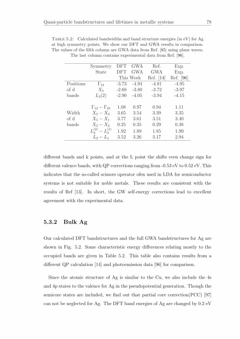
Quasi-particle bandstructures and lifetimes in metallic systems 78
Table 5.2: Calculated bandwidths and band structure energies (in eV) for Agat high symmetry points. We show our DFT and GWA results in comparison.The values of the fifth column are GWA data from Ref. [85] using plane waves.
The last column contains experimental data from Ref. [96].
Symmetry DFT GWA Ref. Exp.State DFT GWA GWA Exp.
This Work Ref. [14] Ref. [96]Positions Γ12 -3.73 -4.94 -4.81 -4.95of d X5 -2.68 -3.80 -3.72 -3.97bands L3(2) -2.90 -4.05 -3.94 -4.15
Γ12 − Γ25 1.08 0.97 0.94 1.11Width X5 −X3 3.65 3.54 3.39 3.35of d X5 −X1 3.77 3.61 3.51 3.40bands X5 −X2 0.25 0.35 0.29 0.38
L(2)3 − L
(1)3 1.92 1.89 1.85 1.99
L3 − L1 3.52 3.26 3.17 2.94
different bands and k points, and at the L point the shifts even change sign for
different valence bands, with QP corrections ranging from -0.53 eV to 0.52 eV. This
indicates that the so-called scissors operator ofen used in LDA for semiconductor
systems is not suitable for noble metals. These results are consistent with the
results of Ref [13]. In short, the GW self-energy corrections lead to excellent
agreement with the experimental data.
5.3.2 Bulk Ag
Our calculated DFT bandstructures and the full GWA bandstructures for Ag are
shown in Fig. 5.2. Some characteristic energy differences relating mostly to the
occupied bands are given in Table 5.2. This table also contains results from a
different QP calculation [14] and photoemission data [96] for comparison.
Since the atomic structure of Ag is similar to the Cu, we also include the 4s
and 4p states to the valence for Ag in the pseudopotential generation. Though the
semicore states are included, we find out that partial core correction(PCC) [97]
can not be neglected for Ag. The DFT band energies of Ag are changed by 0.2 eV

Quasi-particle bandstructures and lifetimes in metallic systems 79
-9-8-7-6-5-4-3-2-1012345678
X1
X3
X2
X5
'
L1
L3
L3
L2'
Ef
L1
GWADFT
KWXL
Ene
rgy(eV
)
Figure 5.2: Calculated band structure for Ag along high-symmetry lines,obtained within DFT (dashed lines) and within GWA (solid lines).
with the inclusion of partial core correction. Our DFT band energy at X5 point is
–2.68 eV, and close to the result of –2.70eV from a full potential calculation (within
LMTO) [83]. Based on the DFT calculation, our calculated d band threshold at the
X5 point is about –3.80 eV within GWA, compared to photoemission data of 3.97
eV. Our quasiparticle results are in quite good agreement with the photoemission
data.
Like in the case of Cu, the Fermi level observes a value of ΣGW − Vxc of about
1.0 eV, while the the top position of the d bands observes ΣGW − Vxc=–0.2 eV.
In total, this results in a downward of shift of about 1.2 eV of the top of the d
bands, and leads to excellent agreement with available photoemission data, as can
be seen from Table 5.2. It can be seen from Fig. 5.2 that the GW corrections do
not act as a rigid shift of the whole occupied bandstructure with respect to the
unoccupied part. This is similar to the situation in Cu. Note, however, that the
bottom of the sp band (at Γ1) is shifted downwards by 0.5 eV for Ag, which is
different from the upwards shift in the case of Cu. For the bandwidths of d bands,
GWA results are closer to experiment than the DFT results are.
We also show calculated data using plane waves reported in Ref. [14] for com-
parison. In spite of the different methods of calculation, our calculated results

Quasi-particle bandstructures and lifetimes in metallic systems 80
are in good overall agreement with the results of Ref. [14] except for some minor
differences. For example, our quasiparticle energies of the d bands deviate from
photoemission data by about 0.1 eV, while the discrepancy is about 0.2 eV in
Ref. [14]. For the case of Ag, we get converged results using only 80 Gaussian
orbitals.
5.4 Quasi-particle lifetimes
Electron and hole dynamics in the bulk as well as at the various surfaces of a solid
play a key role in a great number of physical and chemical phenomena [98, 99]. A
new path for the study of both electron and hole dynamics in the time domain was
opened by the development of the time-resolved two-photon photoemission(TR-
TPPE) technique [17, 18]. Recently first principles calculations of the electron
lifetimes in bulk noble metals have also been published in Refs. [24, 25, 26, 82].
However, many problems related to the approximations employed still remain
unresolved. The common problem is that these calculations are based on the DFT
band energies. Another problem is that the renormalization factors are neglected
in many GW calculations such as Ref. [24, 25, 82]. In fact, the renormalization
factor Z is quite far from the 1.0 used in the ’energy shell’ approximation. We
got an average value of Z = 0.66 for Cu, and Z = 0.74 for Ag. This modifies the
energy of the excitation, and hence, the lifetime.
5.4.1 Bulk Cu
In Fig. 5.3 we compare our calculated lifetimes of electrons for Cu with the
lifetimes of Ref. [27] and experimental data [100]. The dashed lines in Fig. 5.3 are
the lifetimes of Ref. [27] obtained within the so-called Fermi liquid theory(FLT),
the solid line represents the lifetimes of Ref. [27] calculated with plane waves, and
the diamonds are the experimental data of Ref. [94].

Quasi-particle bandstructures and lifetimes in metallic systems 81
0 1 2 3 4 50
10
20
30
40
50
60
70
80
FLTPW
This workExp.
|E-Ef|(eV)
Life
time(
fs)
Figure 5.3: Calculated lifetimes of hot electrons in Cu along high-symmetrylines (circles) in comparison with experimental data (diamonds).[100] The solidand dashed lines denote theoretical results Ref. [27], obtained within GWA and
within Fermi-liquid theory.
In spite of great differences in the methods of calculation, very good agreement is
observed above 1.4 eV between our data and the lifetimes based on the plane waves.
Compared to the lifetimes obtained with plane waves, our calculated lifetimes are
closer to the experimental results at about 1.1 eV. Both our calculated electron
lifetimes of hot electrons and the calculated lifetimes with plane waves are slightly
larger than the results obtained within FLT. This is due to the influence of the d
electrons which provide an additional screening mechanism that is absent in the
jellium model. Below 2 eV the experimental data show a sudden increase. The
origin of the disagreement between calculated results and experimental data was
discussed in Ref. [27], and they explain that the increase is due to the interaction
of the excited electron with its hole in the d bands. As can be seen from Fig. 5.1,
the threshold of d bands is located about 2 eV below the Fermi level. The electrons
at the top of the d bands can be excited by the photon energies widely used in
2PPE experiments. These excited electrons interact with the holes in d bands,
and hence, the electron lifetimes increase at 2 eV for Cu. Gurtubay et al [101]
compute the lifetimes for Cu with full inclusion of exchange and correlation(XC)
effects based on the DFT band energies calculation. This approximation treats

Quasi-particle bandstructures and lifetimes in metallic systems 82
on the same footing XC effects between pairs of electrons within the Fermi sea
(screening electrons) and between the excited hot electron and the Fermi sea.
This corresponds to including the higher order terms in the self-energy operator
beyond the GWA. Electron-hole interaction effects, however, are still not included.
Gurtubay et al conclude that the overall effect of short-range XC is small and GWΓ
linewidths are close to their XC-free G0W0 counterparts. Our calculation, on the
other hand, is based on accurate band energies and include the semicore states. So
the only reason for the discrepancies between theoretical methods and experiments
should be the interactions of the excited electrons with holes in the d bands, which
are not included in the GW calculation.
First principle calculations based on the DFT predict an upper d-band edge
that is located about 1.5 eV below the Fermi level, i.e., about 0.5 eV higher than
observed by photoemission experiments [94]. This indicates that a rigid shift in
the energy axis will occur for the hole lifetime calculations based on the DFT
band energies. The direct influence on the calculated liftimes based on the DFT
band energies is that the calculated values of d-hole lifetimes cannot be directly
compared with experiment. Our calculation is based on the accurate band energies,
the hole energies in Cu are located about 2 eV below the Fermi level, and this is
consistent with the threshold of d bands measured by photoemission experiment,
as shown in Fig. 5.4. It can also be seen from Fig. 5.4 that d holes exhibit a
longer lifetimes than sp electrons with the same excitation energy, in agreement
with experiment. As can be seen from Fig. 5.1, the sp-like bands cross the d bands
below the Fermi level, and a small overlap occurs between the sp states and the
d states. This small overlap between sp bands and d bands is responsible for the
increase of the hole lifetimes at the top of the d bands [82].
In order to find out the influence of quasiparticle corrections on the hole life-
times, we compare our calculated d hole lifetimes with the lifetimes of Ref. [83]
and experiments [86], as shown in Table 5.3. Ref. [83] are the results of GWA,
based on the linear muffin-tin orbitals (LMTO) method. The last column are the
experimental data.

Quasi-particle bandstructures and lifetimes in metallic systems 83
0 1 2 3 4 50
10
20
30
40
50
60
70
80
hole_lifeelectron_life
Lifetim
e(fs)
|E-Ef|(eV)
Figure 5.4: Calculated lifetimes of d holes in Cu, alongt high symmetrylines. For comparison, the electron lifetimes are also presented (solid circles);
open circles represent the hole lifetimes;
Table 5.3: Lifetimes of d holes in Cu (in fs).
Symmetry points This work Ref. [83] Exp. [86]X5 64.4 47.1 33±7X2 53.9 47.5 6.5
Lifetime L3(2) 23.9 23.5of Γ12 22.2 12.6 5.0
d states Γ25 6.2 3.2 3.7L3(1) 6.0 3.02X3 1.7 0.6 2.8
Ref. [86] reported that the calculated lifetimes below 3 eV tend to approach
those predicted by a FEG model of the solid, while the experimental show a
distinct asymptotic behavior at the large binding energies. They attribute this
discrepancy to the failure of the DFT to reproduce the actual band structure of
Cu. As can be seen from Table 5.3, our calculated lifetime at Γ25 (about 3.58
eV below Fermi level) is larger than the experimental data. Both our calculated
lifetime and the lifetime of Ref. [83] at X3(about 4.78 eV below the Fermi level) are
smaller than the experimental data, especially, the calculated lifetime of Ref. [83]
deviate from experiment by 2.2 fs. The LDA eigenvalues have been corrected

Quasi-particle bandstructures and lifetimes in metallic systems 84
0 1 2 3 4 50
20
40
60
80
100
120
FLTPW
This workExp.
Life
time(
fs)
|E-Ef|(eV)
Figure 5.5: Calculated lifetimes of hot electrons in Ag, at high symmetrypoints. solid circles show our results; solid diamonds represent experiments
[100]; solid line and dashed line denote the results of Ref. [27].
before entering the matrix elements of self-energy operator in Ref. [83]. As can
be seen from Table 5.1 and Fig. 5.1, not only the positions of d bands are close
to the experimental data, but also the d band width X5 −X3 is 2.63 eV, which is
in good agreement with the experimental value of 2.79 eV. As can be seen from
Table 5.2, all theoretical lifetimes above Γ25′ are larger than experimental data. So
the quasiparticle corrections to the DFT bandstructure energies are not essential
reasons for the disagreements between theoretical lifetimes and experiments, and
this is consistent with the conclusion of Ref. [87]. In order to accurately describe
lifetimes of holes for noble metals, effects beyond the GW approximation should
be included.
5.4.2 Bulk Ag
Our calculated electron lifetimes for Ag are given in Fig. 5.5 (solid circles). We
compare our results with the results of Ref. [27] based on the plane wave bases
sets, FLT results and experimental data [100].

Quasi-particle bandstructures and lifetimes in metallic systems 85
0 1 2 3 4 5 6 7 80
10
20
30
40
50
60
70
80
90
100
hole_lifeelectron_life
Lifetim
e(fs)
|E-Ef|(eV)
Figure 5.6: Calculated lifetimes of d holes in Ag, at high symmetry points.open circles represent the lifetime of holes; solid circles depict the lifetime of
electrons.
Our calculated lifetimes of electrons in Ag are in good agreement with the results
from literature. As can be seen from Fig. 5.5, our results are closer to the results
obtained within FLT than the theoretical lifetimes from plane waves. As can be
seen from Fig. 5.2, the d band threshold locates about 3.80 eV below the Fermi
level. This indicates that for all excited electrons below 3.80 eV the relaxation
of the hot electrons can not excite the elctrons in the d bands, and lead to FLT
behavior of Ag. Contrary to the case of Cu, the experimental data for Ag do not
show a sudden increase at small energies, due to the fact that the d band threshold
is about 3.80 eV below the Fermi level, as shown in Fig. 5.2, and no d electrons are
excited for the photon energies widely used in 2PPE experiments. This indicates
that the the electron lifetimes of Ag are mainly attributed to the electron-electron
interactions.
As can be seen from Fig. 5.6, the hole lifetimes of d states are located about 3.8
eV below the Fermi level, which is in agreement with the experimental threshold
of d bands. It can also be seen from Fig. 5.6 that the hole lifetimes are larger than
the electron lifetimes, which is in agreement with experiments [102], and this is
similar to the case of Cu. The band structure in Fig. 5.2 presents a small overlap

Quasi-particle bandstructures and lifetimes in metallic systems 86
Table 5.4: Lifetimes of d holes for Ag (in fs)
Symmetry points This work Exp. [102]X5 68.82 22X2 74.25 12X3 2.19X1 1.95 2.0
between d and sp states at the top of d bands(3.8 eV below the Fermi level) and
large overlaps between d bands at deeper energy below Fermi level. The small
overlap yields a dramatic increase of the hole lifetimes, especially, at the top of
d bands. As the d hole energy decreases, large overlap between d bands yields a
rapid decrease of hole lifetimes.
As can be seen from Table 5.4, our calculated lifetime is about 68 fs at the
upper edge of d bands(X5 point, as shown in Fig. 5.2), while the experimental
[102] value is 22 fs. Large discrepancy appears at X2 point. For the states at X1,
good agreement is observed between our calculated lifetime and lifetime measured
by experiment. In spite of the large quasiparticle corrections of the d bands for
Ag(1.2 eV), our calculated hole lifetimes for Ag still deviate from experiment, and
this is similar to the case of Cu.
It is well known that the GW approximation accounts well for long-range screen-
ing. Short range interactions such as electron-hole and hole-hole interations near
the Fermi level may be crucial for the hole lifetimes in the case of noble metals and
electron lifetimes in the case of Cu. With increasing distance to the Fermi level,
the long range interactions dominate the scattering mechanism and thus lead to
good agreement with the experiments.
5.5 Image potential state lifetimes in Cu(100)
At a metal surface one can find two types of electronic states which don’t exists
in a bulk metal. According to their charge density localization relative to the

Quasi-particle bandstructures and lifetimes in metallic systems 87
Figure 5.7: Sketch of the electric field lines for an electron at a distance zin front of a conducting metal surface (solid lines). An positive image charge is
inside the solid at -z(field lines are represented by dashed lines).
surface atomic layer, these states at a metal surface are intrinsic surface states
and image-potential states, respectively. Tamm [103] and Shockley [104] predicted
theoretically the so-called intrinsic surface states, which are localized mainly at the
surface atomic layer. Echenique and Pendry [105] predicted the image potential
states, which are localized mostly in the vacuum region if the bulk meterial has a
band gap near the vacuum level(as given, e.g., for the Cu(100) suface).
The understanding of image potential states is rather simple. An electron at
a distance z in front of a conducting metal surfaces moves in a Coulomb like
attractive image potential, which can be expressed as
V (z) = − e2
8πε0z(5.14)
The attractive image potential is produced by the electron interaction with a
positive(mirror image) charge at a distance z inside the metal, as can be seen from
Fig. 5.7. If the metal has a band gap near the vacuum level, then an electron
below the vacuum level usually transfered from the bulk by a laser may be trapped
by the attractive potential. The electronic states of the trapped electron form a
Quasi-particle bandstructures and lifetimes in metallic systems 88
hydrogen like Rydberg series with energies En
En =−0.85eV
(n+ a)2, n = 1, 2, . . . (5.15)
where a is a quantum defect depending on both the energy gap position and width
and also on the posititon of image state relative to the gap [105, 106].
5.5.1 Computational details and discussion of results
Here, the image potential state lifetimes for the Cu(100) surface have been evalu-
ated within the many-body-perturbation theory. Our Cu(100) geometry contains
4 atomic layer and 26 vacuum layers, and the supercell has 1×1 periodicity. We
evaluate the lifetimes from the imaginary part of the electron self energy, which
we compute within the GW approximation. Similar to bulk Cu, localized Gaus-
sian basis sets have been used for speeding up and reducing the computational
cost of both DFT and GW calculations. These basis functions have the form
of atomic orbitals, but are forced to be zero beyond a given confinement radius.
For the image potential states of Cu(100), the n = 1 probability density has a
maximum at 3.8 A outside the crystal edge(the outermost atomic layer of the
Cu(100)) [107]. In order to describe the image potential states in the vacuum
region, we add ten ’virtual’ atomic layers in the vacuum region above the surface,
up to 23 A in height. The layer distances between two ’virtual’ atomic layers are
the same as the layer distances of bulk region. Moreover, for the DFT and GWA
calculations, we use the decaying p-type orbitals for every ’virtual’ atom in the
vacuum region. In addition, the LDA and GWA Gaussian basis sets designed for
the bulk Cu calculation are used directly for the bulk region atom of Cu(100). In
order to calculate the dynamically screened Coulomb interaction(W = ε−1v), one
should calculate firstly the polarization P (see Sec.5.2), which is convoluted with
the Coulomb interaction v yielding the dielectric function ε = 1− vP .
Finally, the image potential state energies and lifetimes of Cu(100) with quan-
tum number n = 1 and n = 2 have been calculated. Our calculated quasi-particle

Quasi-particle bandstructures and lifetimes in metallic systems 89
Table 5.5: Calculated image state lifetimes of n = 1, 2 and experimentalresults [108], as well as the theoretical results from literature using a model
potential, at the Γ point.
quantum number This work(fs) Exp. [108](fs) Ref. [107](fs)n = 1 31 40 ± 6 30n = 2 109 110 ± 10 132
corrections for image potential states are zero. This results in larger image poten-
tial state energies by 0.5 eV, as compared to experimental results, which are 4.04
eV and 4.45 eV for n = 1 and n = 2 states, respectively. The discrepancies between
calculated image potential state energies and experimental results should be origi-
nated from the neglecting of the off-diagonal matrix elements of the self-energy Σ.
Our calculated image potential state lifetimes of Cu(100) are presented in Table
5.5, together with experimental results and the theoretical results calculated from
a model potential, and the calculated image state lifetimes using the pseudopoten-
tial methods are in agreement with the experimental results and the theoretical
results by using a model one-dimensional potential. This also demonstrates that
the quasi-particle corrections have minor influences on the lifetimes(See the dis-
cussion in the last section) For the one dimensional model potential method, ten
parameters should be considered carefully to construct the one-dimensional poten-
tial. Most of the parameters are determined from the requirement of continuity
of the potential and its first derivative everywhere in space, but four parameters
of them are adjustable(i.e. the four independent parameters have to be fitted
to the experimental parameters or the parameters from first-principles calcula-
tions). So the one-dimensional potential method is a semi-empirical method. For
our method, taking advantage of the efficienct Gaussian basis sets to expand the
wave functions both for DFT and GWA, we can perform the image potential
state lifetimes calculation using the pseudopotential instead of the semi-empirical
one-dimensional potential.

Quasi-particle bandstructures and lifetimes in metallic systems 90
5.6 Summary
In conclusion, we have performed the first ab initio calculations of quasiparticle
bandstructures and lifetimes for noble metals Cu and Ag using efficient Gaussian
orbital basis set. With the use of localized Gaussian orbitals, only less than 80
Gaussian orbitals both for the LDA basis sets and the GWA basis sets are needed,
instead of thousands of plane waves. The traditional LDA calculations for Cu and
Ag usually place the d bands too close to the Fermi level, especially for the Ag.
The well-known discrepancies between experiments and DFT bandstructures are
almost completely corrected by GW calculations. It turns out that Hedin’s GW
approximation is successful for the description of band-structures of noble metals.
Based on the accurate bandstructures, the lifetimes of electrons and holes in Cu
and Ag have been calculated. Comparing with experimental data, the quasiparticle
corrections do not lead to qualitative improvements of the quasiparticle lifetimes.
It is well known that the GW approach well accounts for the long range screening,
while short range interactions which are more important for noble metals are not
well described. Therefore, it is probable that the improvement of the calculated
lifetimes within GW approximation for d materials can be achieved by inclusion of
higher terms of the many body perturbation, i.e., the short-range screening such
as electron-hole and hole-hole interactions should be included when we evaluate
the self-energy operator. In addition, our calculated image potential state lifetimes
of Cu(100) with the quantum number n = 1, 2 using the pseudopotential method
are in good agreement with experimental results.
Appendix A
Derivation of some equations in
this thesis
A.1 The motion of Green’s function
The many particle Hamitonian can be written as
H =∑
i
[−∇2i
2m+ Vext(ri)] +
1
2
∑ij
v(ri, rj) (A.1)
where Vexc(r is the external potential generated by the atomic nuclei, v(r1, r2) =
e2(4πε0|r1 − r2|) is the coulomb interaction, and ε0 is the vacuum dielectric
constant.
With the field operator introduced in Sec. 4.2. the above equation can be
rewritten as
H =
∫ψ+(r1)h0(r1)ψ(r1)dr1 +
1
2
∫ψ+(r1)ψ
+(r2)v(r1, r2)ψ(r2)ψ(r1)dr1dr2
(A.2)
where h0 is the one-particle term of Hamitonian h0(r) = −∇2i2 + Vext(r)
91

Appendix 92
In the Heisenberg picture, the equations of motion for the field operators are:
i∂
∂t1ψ(1) = h0(1)ψ(1) +
∫d2v(1, 2)ψ+(2)ψ(2)ψ(1)
i∂
∂t1ψ+(1) = −h0(1)ψ+(1)− ψ+(1)
∫d2v(1, 2)ψ+(2)ψ(2) (A.3)
The Green’s function is given by
G(1, 2) = −i[θ(t1 − t2)〈N |ψ(1)ψ+(2)|N〉 − θ(t2 − t1)〈N |ψ+(2)ψ(1)|N〉] (A.4)
The derivative ∂∂t1
of the first term in the right-hand-side of above equation is
expressed as
∂∂t1
[θ(t1 − t2)〈N |ψ(1)ψ+(2)|N〉]= [
∂
∂t1θ(t1 − t2)]〈N |ψ(1)ψ+(2)|N〉+ θ(t1 − t2)〈N | ∂
∂t1ψ(1)ψ+(2) (A.5)
Similarly, it is easy to obtain the derivative for the second term of Eqs.(A4). By
using the following relation:
∂
∂t1θ(t1 − t2) = − ∂
∂t1θ(t2 − t1) = δ(t1 − t2) (A.6)
and summing up the derivatives of the two terms in Eqs.(A4), we can obtain:
∂
∂t1G(1, 2) = δ(1, 2)− i〈N |T [i
∂
∂t1ψ(1)ψ+(2)]|N〉 (A.7)
where T is the stands for the Wick time-ordering operator(see sec. 4.2). Using
the Eqs.(A2) for the field operators in the above equation, we can obtain:
∂
∂t1G(1, 2) = δ(1, 2) − ih0(1)〈N |T [ψ(1)ψ+(2)]|N〉
− i
∫d3v(1, 3)〈N |T [ψ+(3)ψ(3)ψ(1)ψ+(2)]|N〉 (A.8)

Appendix 93
We define the two particle Green’s function as:
G2(1, 2, 3, 4) = (−i)2〈N |T [ψ(1)ψ(2)ψ+(4)ψ+(3)]|N〉 (A.9)
Finally, the motion of Green’s function is expressed as
[i∂
∂t1− h0(1)]G(1, 2) = δ(1, 2)− i
∫d3v(1, 3)G2(1, 3, 2, 3
+) (A.10)
A.2 Schwinger’s functional derivative
If a system experiences a small time-dependent external perturbing potential
Uper(r1, r2, t) is given by
Htot = H + H1 = H +
∫dr1dr2ψ
+(r1, t+)Uper(r1, r2, t)ψ(r2, t) (A.11)
where ψ and ψ+ are field operators(see Sec. 4.2). The perturbation Uper will be
made vanish at the end of the derivation.
Then the one paricle Green’s function becomes
G(1, 2) = −i〈N |T [Sψ(1)ψ+(2)]|N〉〈N |T [S]|N (A.12)
where S is the time evolution operator, and is given by the following relation
[76, 109]:
S(t) = exp(−i∫ ∞
−∞dtH1(t))
= exp[−i∫ ∞
−∞dt
∫dr1dr2ψ
+(r1, t+)Uper(r1, r2, t)ψ(r2, t)] (A.13)
U = 0 corresponds to the definition of one-particle Green’s function. The entire U
dependence of this generalized Green’s function lies in the time evolution operator

Appendix 94
S. Therefore:
δG(1, 2) = −i〈N |T [δSψ(1)ψ+(2)]|N〉〈N |T [S]|N +G(1, 2)
〈N |T [δS]|N〉〈N |T [S]|N (A.14)
and the variation δS can be evaluated as
T [δS] = −iT [S
∫ ∞
−∞dt
∫dr3dr4ψ
+(r3, t+)δUper(r3, r4, t)ψ(r4, t)] (A.15)
Inserting Eqs.(A15) to Eqs.(A14), one can get the following relation:
δG(1, 2) = −∫ ∞
−∞dt
∫dr3dr4[G2(1, r4t; 2, r3t
+)]−G(1, 2)G(r4t, r3t+) (A.16)
Finally, the final formula of the Schwinger’s functional derivative is expressed as
δG(1, 2
δUper(3, 4)= G(1, 2)G(4, 3)−G2(1, 4; 2, 3) (A.17)
Appendix B
Detailed information for the
pseudopotential generation of Cu
and Ag
B.1 Pseudopotential generation
One usually consider a configuration 3d104s1 for Cu in the DFT calculations. This
configuration for Cu can yield good results for some quantities in the DFT calcu-
lations due to the large(' 66eV ) energy seperation between the 3d and 3s states.
However, the the 3d wave functions are compact and overlap significantly with
the 3s and 3p semi-core states. This effect is larger if one performs a GW calcula-
tion. For instance, the inclusion of semi-core 3s and 3p into the valence leads to a
very defferent values of 〈Σnkx − V nk
xc 〉, and improves considerable the quasi-particle
energies [13]. Therefore, an obvious solution would be include those 3s and 3p
semi-core states as part of the valence in the pseudopotential generation scheme.
That would require a somewhat larger energy cutoff in the plane wave expansion
with repect to the 3d electrons and a larger number of electrons in the valence, cor-
responding to a manageable increase in the necessary computing resources. For the
most pseudopotential program, one can only have a single pseudowave-function of
95
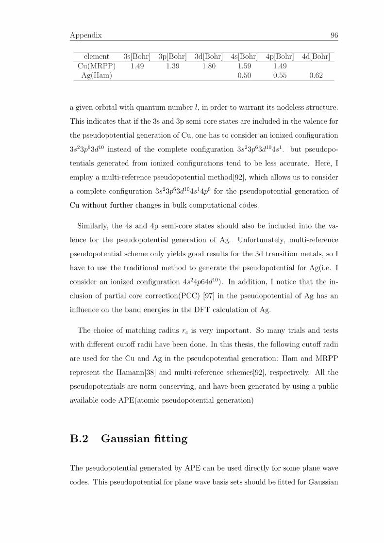
Appendix 96
element 3s[Bohr] 3p[Bohr] 3d[Bohr] 4s[Bohr] 4p[Bohr] 4d[Bohr]Cu(MRPP) 1.49 1.39 1.80 1.59 1.49Ag(Ham) 0.50 0.55 0.62
a given orbital with quantum number l, in order to warrant its nodeless structure.
This indicates that if the 3s and 3p semi-core states are included in the valence for
the pseudopotential generation of Cu, one has to consider an ionized configuration
3s23p63d10 instead of the complete configuration 3s23p63d104s1. but pseudopo-
tentials generated from ionized configurations tend to be less accurate. Here, I
employ a multi-reference pseudopotential method[92], which allows us to consider
a complete configuration 3s23p63d104s14p0 for the pseudopotential generation of
Cu without further changes in bulk computational codes.
Similarly, the 4s and 4p semi-core states should also be included into the va-
lence for the pseudopotential generation of Ag. Unfortunately, multi-reference
pseudopotential scheme only yields good results for the 3d transition metals, so I
have to use the traditional method to generate the pseudopotential for Ag(i.e. I
consider an ionized configuration 4s24p64d10). In addition, I notice that the in-
clusion of partial core correction(PCC) [97] in the pseudopotential of Ag has an
influence on the band energies in the DFT calculation of Ag.
The choice of matching radius rc is very important. So many trials and tests
with different cutoff radii have been done. In this thesis, the following cutoff radii
are used for the Cu and Ag in the pseudopotential generation: Ham and MRPP
represent the Hamann[38] and multi-reference schemes[92], respectively. All the
pseudopotentials are norm-conserving, and have been generated by using a public
available code APE(atomic pseudopotential generation)
B.2 Gaussian fitting
The pseudopotential generated by APE can be used directly for some plane wave
codes. This pseudopotential for plane wave basis sets should be fitted for Gaussian

Appendix 97
basis sets, since we employ a localized Gassian basis sets in the quasi-particle
bandstructures and lifetimes calculation.
Vl = Vloc(r) + ∆Vl (B.1)
The core potential is thought of as originating from Gaussian-type effective core
charges:
Vloc(r) = −Zv
r
2∑i=1
cierf[(√αi
loc)r] (B.2)
where Zv is the Valence charge, c1 + c2 = 1, erf is the error function, given by
erf(x) =2
π
∫ x
0
exp(−t2)dt (B.3)
The remaining potential is expanded in Gaussian-type functions as
∆Vl =n∑
i=1
(Ai + Ai+n)e−αli·r2
(B.4)
where Ai and Ai+n are the linear coeffients, which correspond to the decay con-
stants αli for each angular momentum l value. Here I set n = 5, and n = 4 for Cu
and Ag, respectively.

Acknowledgements
First of all I would like to express my sincere gratitude to my supervisor, Prof. Dr.
Michael Rohlfing, for his constant and invaluable surport during my PhD study.
I have learned a lot from his intelligent guidance, valuable discussions in the last
three years.
My special thanks go to Dr. Yuchen Ma. His insight discussions and interpre-
tation of many physics and computational problems helped me move on and gave
me valuable hints. I am indebted to Dr. Marcin Kaczmarski, who gave me a lot
of helps for handling computer problems.
I would like to say my thanks to Dr. Heidrun Elfering, the former secretary of
the Promotion program, who helped me to handle various problems in the past
years.
I am very thankful to my wife. In order to help me to finish my thesis, she
takes care of my child alone. I am grateful to my parents, sister and brother who
surported me throughout these three years and before.
Finally, I would like to thank all the persons who surported and helped me
during my Ph.D study.
This work has been supported financially in the framework of PhD program
”Synthesis and Characterization of Surfaces and Interfaces assembled from Clus-
ters and Molecules”. The financial support is also gratefully acknowledged.
98

Eidesstattliche Erklarung
Hiermit erklare ich, dass ich die vorliegende Arbeit selbststandig und ohne fremde
Hilfe verfasst, andere als die von mir angegebenen Quellen und Hilfsmittel nicht
benutzt und die den benutzten Werken wortlich oder inhaltlich entnommenen
Stellen als solche kenntlich gemacht und keine vorherigen Promotionsversuche un-
ternommen habe.
Osnabruck, 17.11.2009
Zhijun Yi
99

Bibliography
[1] W. Kohn and L. J. Sham, Phys. Rev. 140, A 1133 (1965).
[2] R. M. Dreizler and E. K. U. Gross, Density Functional Theory (Springer-
Verlag, Berlin, 1990); R. G. Parr and W. Yang, Density Functional Theory
of Atoms and Molecules (Oxford, New York, 1989).
[3] D. M. Ceperley and B. J. Alder, Phys. Rev. Lett. 45, 566 (1980).
[4] A. D. Becke, Phys. Rev. A 38, 3098 (1988).
[5] J. P. Perdew, K. Burke, and M. Ernzerhof, Phys. Rev. Lett. 77, 3865 (1996).
[6] D. Hartree, Proc. Cambridge Philos. Soc. 24, 89 (1928).
[7] V. Fock, Z. Phys. 61, 126 (1930).
[8] V. N. Strocov et al., Phys. Rev. Lett. 81, 4943 (1998); Phys. Rev. B 63, 205108
(2001).
[9] L. D. Landau, Soviet Phys. JETP. 3, 920 (1957); Soviet Phys. JETP. 5, 101
(1957).
[10] L. Luttinger and J. Ward, Phys. Rev. 118, 1417 (1960).
[11] L. Hedin, Phys. Rev. 139, A796 (1965).
[12] F. Aryasetiawan, Phys. Rev. B 46, 13051 (1992).
[13] A. Marini, G. Onida, and R. Del Sole, Phys. Rev. Lett. 88, 016403 (2002).
[14] A. Marini, R. Del Sole, and G. Onida, Phys. Rev. B 66, 115101 (2002).
[15] E. V. Chulkov, A. G. Borisov, et. al. Echenique, Chem. Rev. Washington, D.
C. 106, 4160 2006.
100

[16] J. B. Pendry, in Photoemission and the Electronic Properties of Surfaces, B.
Feuerbacher, B. Fitton, R.F. Willis(Eds.), Wiley, 1978.
[17] J. Bokor, Science 246, 1130 (1989).
[18] R. Haight, Surf. Sci. Rep. 21, 275 (1995).
[19] P. M. Echenique et al., Chem. Phys. 251, 1 (2000), and references therein.
[20] R. H. Ritchie, Phys. Rev. 114, 644 (1959).
[21] J. J. Quinn, Phys. Rev. 126, 1453 (1962); J. C. Shelton, Surf. Sci. 44, 305
(1974).
[22] R. H. Ritchie and J. C. Ashley, J. Phys. Chem. Solids 26, 1689 (1963); L.
Kleinman, Phys. Rev. B 3, 2982 (1976); D. R. Penn, Phys. Rev. B 13, 5248
(1976).
[23] D. R. Penn, Phys. Rev. B 22, 2677 (1980).
[24] I. Campillo, J.M. Pitarke, A. Rubio, E. Zarate, and P.M. Echenique, Phys.
Rev. Lett. 83, 2230 (1999).
[25] I. Campillo, V.M. Silkin, J.M. Pitarke, E.V. Chulkov, A. Rubio, and P.M.
Echenique, Phys. Rev. B 61, 13 484 (2000).
[26] W.-D. Schone, R. Keyling, M. Bandic, and W. Ekardt, Phys. Rev. B 60, 8616
(1999).
[27] R. Keyling, W.-D. Schone, and W. Ekardt, Phys. Rev. B. 61, 1670(2000).
[28] J. Tersoff and D. R. Hamann, Phys. Rev. B 31, 805 (1985).
[29] L. S. Thomas, Proc. Cambridge Philos. Soc. 23, 542 (1927).
[30] E. Fermi, Z. Phys. 48, 73 (1928).
[31] E. Teller, Rev. Mod. Phys. 34, 627 (1962).
[32] P. Hohenberg and W. Khon, Phys. Rev. 136, B864 (1964).
[33] L. Fetter and J. D. Walecka Quantum theory of Many-Body Systems,
McGraw-Hill, New York, N.Y. 1981.
[34] S. H. Vosko, L. Wilk and M. Nusair, Can. J. Phys. 58, 1200 (1980).

[35] J. P. Perdew and A. Zunger, Phys. Rev. B 23, 5048 (1981).
[36] L. A. Cole and J. P. Perdew, Phys. Rev. A 25, 1265 (1982).
[37] J. P. Perdew and Yue Wang, Phys. Rev. B 45, 13244 (1992).
[38] D. R. Hamann, M. Schluter, and C. Chiang. Phys. Rev. Lett. 43, 1494 (1979).
[39] G. B. Bachelet, D. R. Hamann, and C. Chiang. Phys. Rev. B 26, 4199 (1982).
[40] L. Kleinman and D. M. Bylander, Phys. Rev. Lett. 48, 1425 (1982).
[41] A. Mordecai, Nonlinear Programming: Analysis and Methods (Dover, New
York, 2003).
[42] H. Hellmann, Einfuhrung in die Quantenchemie (Franz Deuticke, Leipzig,
1937), p. 285
[43] R. P. Feynman, Phys. Rev. 56, 346 (1939).
[44] D. L. Chadi and M. L. Cohen, Phys. Rev. B 8, 5747 (1973).
[45] H. J. Monkhorst and J. D. Pack, Phys. Rev. B 13, 5188 (1976).
[46] A. Baldereschi, Phys. Rev. B 7, 5212 (1973).
[47] D.V. Lang and R. A. Logan, Phys. Rev. Lett. 39, 635 (1977).
[48] R. J. Nelson, Appl. Phys. Lett. 31, 351 (1977).
[49] P. M. Mooney, J. Appl. Phys. 67, R1 (1990).
[50] D. K. Maude, J. C. Portal, L. Dmowski, T. Foster, L. Eaves, M. Nathan, M.
Heiblum, J. J. Harris and R. B. Beall, Phys. Rev. Lett. 59, 815 (1987).
[51] D. J. Chadi and K. J. Chang, Phys. Rev. Lett. 61, 873 (1988).
[52] D. J. Chadi and K. J. Chang, Phys. Rev. B 39, 10063 (1989).
[53] S. B. Zhang and D. J. Chadi, Phys. Rev. B 42, 7174 (1990).
[54] M. H. Du and S. B. Zhang, Phys. Rev. B 72, 075210 (2005).
[55] P. M. Mooney, W. Wilkening, U. Kaufmann, and T. F. Kuech, Phys. Rev. B
39 5554 (1989).

[56] H. J. Bardeleben, J. C. Bourgoin, P. Basmasji, and P. Gibart, Phys. Rev. B
40 5892 (1989).
[57] K. Khachaturyan, E. R. Weber, M. G. Crawford, and G. E. Stillmann, J.
Electron. Mater 20 59 (1991).
[58] L.W. Wang and J. Li, Phys. Rev. B 69, 153302 (2004).
[59] J. Li and S. H. Wei, Phys. Rev. Lett. 94, 185501 (2005).
[60] G. Binnig, H. Rohrer, C. Gerber, and E. Weibel, Phys. Rev. Lett. 50, 120
(1983).
[61] G. Cox, D. Szynka, U. Poppe, K. H. Graf, K. Urban, C. Kisielowski-
Kemmerich, J. Krger, and H. Alexander, Phys. Rev. Lett. 64 2402 (1990).
[62] R. M. Feenstra, J. M. Woodall, and G. D. Pettit, Phys. Rev. Lett. 71,
1176(1993).
[63] J. F. Zheng, X. Liu, N. Newman, E. R. Weber, D. F. Ogletree, and M.
Salmeron, Phys, Rev. Lett. 72, 1490(1994).
[64] R. B. Capaz, K. Cho, and J. D. Joannopoulos, Phys. Rev. Lett. 75, 1811
(1995).
[65] J. Wang, T. A. Arias, J. D. Joannopoulos, G. W. Turner, and O. L. Alerhand,
Phys. Rev. B 47, 10329 (1993).
[66] X. Duan, M. Peressi, and S. Baroni, Phys. Rev. B 72 08534 (2005).
[67] S. Baroni, A. Dal Corso, S. de Gironcoli, P. Giannozzi, C. Cavazzoni, G.
Ballabio, S. Scandolo, G. Chiarotti, P. Focher, A. Pasquarello, K. Laasonen,
A. Trave, R. Car, N. Marzari, and A. Kokalj, http://www.pwscf.org.
[68] S. H. Wei and S. B. Zhang, Phys. Rev. B 66, 155211 (2002).
[69] G. Makov and M. C. Payne, Phys. Rev. B 51, 4014 (1995).
[70] Ph. Ebert, B. Engels, P. Richard, K. Schroeder, S. Blgel, C. Domke, M.
Heinrich, and K. Urban, Phys. Rev. Lett. 77, 2997 (1996)
[71] R. M. Feenstra, and J. A. Stroscio, J. Tersoff, and A. P. Fein, Phys. Rev.
Lett. 58, 1192 (1987).

[72] K. Tecichmann, M. Wenderoth, S. Loth and R. G. Ulbrich, Phys. Rev. Lett.
101, 076103 (2008).
[73] A. L. Fetter and J. D. Walecka, Quantum Theory of Many-Particle Systems
(Dover,New York, 2003).
[74] V. M. Galitskii and A. B. Migdal, Sov. Phys. JETP 7, 96 (1958).
[75] J. Schwinger, Proc. Nat. Accad. Sci. 37, 452 (1951).
[76] E. K. U. Gross, E. Runge, and O. Heinonen, Many-Particule Theory (Adam
Hilger, Bristol, Philadelphia and New-York, 1986).
[77] J. Hubbard, Proc. Roy. Soc. A240, 539 (1957).
[78] P. M. Morse and H. Feshbach, Methods of Theoretical Physics, McGraw-Hill,
New York (1953), pp 864-866
[79] P. C. Martin, Measurements and correlation functions (Gordon and Breach,
New York, 1968).
[80] R. Matzdorf et al., Appl. Phys. B 68, 393 (1999).
[81] H. Petek, H. Nagano, S. Ogawa, Appl. Phys. B 68, 369 (1998).
[82] I. Campillo, A. Rubio, J.M. Pitarke, A. Goldmann, and P.M. Echenique,
Phys. Rev. Lett. 85, 3241(2000).
[83] V. P. Zhukov, F. Aryasetiawan, E.V. Chulkov, I.G. de Gurtubay,and P.M.
Echenique, Phys. Rev. B 64, 195122 (2001).
[84] M. Rohlfing, P. Kruger and Johannes Pollmann, Phys. Rev. B. 52, 1905
(1995).
[85] A. Marini, R. Del Sole, A. Rubio, and G. Onida, Phys. Rev. B 66, 161104
(2002).
[86] A. Gerlach, K. Berge, A. Goldmann, I. Campillo, A. Rubio, J.M. Pitarke,
and P.M. Echenique, Phys. Rev. B 64, 085423 (2001).
[87] V. P. Zhukov, E. V. Chulkov, and P.M. Echenique, Phys. Rev. B 68, 045102
(2003).

[88] P.M. Echenique, R. Berndt, E.V. Chulkov, T. Fauster, A. Goldmann, U.
Hofer, Surf. Sci. Rep. 52 (2004) 219.
[89] V.M. Silkin, T. Balasubramanian, E.V. Chulkov, A. Rubio, P.M. Echenique,
Phys. Rev. B64 (2001) 085334.
[90] E. V. Chulkov, V. M. Silkin, and P. M. Echenique, Surf. Sci. 391, L1217
(1997).
[91] M. Rohlfing, P. Kruger and Johannes Pollmann, Phys. Rev. Lett. 75, 3489
(1995).
[92] Carlos L. Reis, J. M. Pacheco and Jose Luis Martins, Phys. Rev. B 68, 155111
(2003).
[93] M. S. Hybertsen, S. G, Louie, Phys. Rev. B 34, 5390 (1986).
[94] S. Ogawa, H. Nagano, and H. Peter, Phys. Rev. B 55, 10869(1997).
[95] R. Courths and S. Hufner, Phys. Rep. 112, 53 (1984).
[96] G. Fuster, J.M. Tyler, N. E. Brener, J. Callaway, and D. Bagayoko, Phys.
Rev. B 42, 7322(1990).
[97] S. G. Louie, S. Froyen, and M. L. Cohen, Phys. Rev. B 26, 1738(1982).
[98] H. Petek and S. Ogawa, Prog. Surf. Sci. 56, 239 (1998).
[99] Laser Spectroscopy and Photochemistry on Metal Surfaces, edited by H.L.
Dai and W. Ho(World Scientific, Singapore, (1995).
[100] M. Wolf and M. Aeschlimann, Phys. Bl. 54, 145(1998).
[101] I. G. Gurtubay, J. M. Pitarke and P. M. Echenique, Phys. Rev. B 69, 245106
(2004).
[102] A. Gerlach, K. Berge a, T. Michalke et al., Sur. Sci. 497, 311 (2002).
[103] I. E. Tamm. Uber eine mogliche Art der Elektronenbindung an Kristal-
loberflachen. Z. Phys., 76, 849 (1932).
[104] W. Shockley. Phys. Rev., 56, 317 (1939).
[105] P. M. Echenique and J. B. Pendry, J. Phys. C., 11, 2065 (1978).

[106] J. Rundgren, G. Malmstrom, J. Phys. C10 4671, (1977).
[107] E. V. Chulkov, I. I. Sarria, V. M. Silkin, J. M. Pitarke, P. M. Echenique,
Phys. Rev. Lett. 80, 4947 (1998).
[108] U. Hofer, I. L. Shumay, Ch. Reub, U. Thomann, W. Wallauer, and Th.
Fauster, Science 277, 1480 (1997).
[109] G. Strinati, Rivista del Nuovo Cimento 11, 1 (1988).