Embed Size (px)
Citation preview

AB INITIO STUDY OF COHESIVE,ELECTRONIC AND ELASTIC PROPERTIES
OF ORDERED CUBIC-BASED Mg-Li ALLOYS
A thesis presented
by
Maje Jacob Phasha
to
The Faculty of Sciences, Health and Agriculturein fulfillment of the requirements
for the degree of
Master of Sciencein the subject of
PhysicsUniversity of Limpopo (Turfloop Campus)
(Former University of the North)Sovenga, South Africa
Supervisor: Professor P.E. NgoepeCo-Supervisor: Professor D.G. Pettifor
c© [2005] by [Maje Jacob Phasha]
[May] [2005]

ABSTRACT
Self-consistent electronic structure calculations have been performedon ordered
cubic-based magnesium-lithium (Mgx-Li1−x) alloys spanning the concentration range
0 ≤ x ≤ 1, using an ab initio plane wave pseudopotential (PWP) method. The first
principle pseudopotential planewave approach is used within the local density approxi-
mation (LDA) and generalized-gradient approximation (GGA)of the density functional
theory (DFT) framework. We have calculated the binding energy curves and the sys-
tematic trends in various cohesive and elastic properties at zero temperature, as a func-
tion of Li concentration. The calculated equilibrium lattice parametersshow a large
deviation from Vegard’s rule in the Li-rich region whilst the bulk moduli decrease
monotonically with increase in Li concentration. The heats of formation for differ-
ent ground state superstructures predict that the DO3, B2 and DO22 structures would
be the most stable at absolute zero amongst various phases having the Mg3Li, MgLi
and MgLi3 compositions, respectively. This stability is reflected in the electronic den-
sity of states (DOS). Because of the special significance of the isotropicbulk modulus,
shear modulus, Young’s modulus and Poisson’s ratio for technological and engineer-
ing applications, we have also calculated these quantities from the elastic constants.
The elastic constants indicate the softness of the material as more Li is added with

the bcc-based phases becoming mechanically less stable for Li concentration less than
50%. Our results show good agreement within the estimated uncertainty with both
experimental and previous theoretical results.

DECLARATION
I declare that the dissertation hereby submitted to the University of Limpopo for
the degree of Master of Science has not previously been submitted by me for a degree
at this or any other university, that it is my own work both in design and execution, and
that all material contained therein has been duly acknowledged.
Maje Jacob Phasha

DEDICATION
This piece of work is dedicated to the following:
My parents,Maria Ramasela & William Madimetja Phasha
My aunt,Esther Masekopo & uncle,Andrew Somchesa Mahlangu
My two beloved brothers,Malose Thona & Frekkie Mashou Phasha
My grandfather,Jones Thapedi Matlou, all my Ancestors &
their King Dashe.
Ka Maatla!!!

ACKNOWLEDGEMENTS
I would like to thank various people and organizations who contributed in dif-
ferent ways to make this work a success. I highly appreciate and acknowledge the
guidance and courageous support of Prof. P.E. Ngoepe throughout the entire process
of this work.
I would like to send my sincere gratitude to Prof. D.G. Pettifor and Dr. D.
Nguyen-Mann for their guiding and stimulating discussions as well as valuableand
helpful inputs. All members of MMC and Materials Modelling Laboratory (MML),
Department of Materials, Oxford University, who contributed in various forms to mak-
ing this work come through are greatly acknowledged.
The financial support from The National Research Foundation (NRF) of South
Africa-Royal Society (RS) of Great Britain collaboration and Councilfor the Scientific
and Industrial Research (CSIR) is greatly acknowledged. The University of the North
for providing the state of art Materials Modelling Center (MMC), which is within the
School of Physical and Mineral Sciences of Facaulty of Health, Science and Agricul-
ture, with excellent facilities to enable us to perform all our calculations in this work.

Mostly, I am very much thankful to my family and friends who stood by me
during difficult and challenging times and also for their patience throughout my period
of study.
Lastly, I am greatful to everyone who might have contributed to the success of
this work in one way or the other.

Table of Contents
1.1 List of Figures . . . . . . . . . . . . . . . . . . . . . . . . . . . . . . . . . . . . . . . .. . . . . . . . . . . . . . . . . . 0
1.2 List of Tables . . . . . . . . . . . . . . . . . . . . . . . . . . . . . . . . . . . . . . . .. . . . . . . . . . . . . . . . . . . 1
1 INTRODUCTION . . . . . . . . . . . . . . . . . . . . . . . . . . . . . . . . . . . . . . . . . . . . . . . . . . .. . . 1
1.1 Background . . . . . . . . . . . . . . . . . . . . . . . . . . . . . . . . . . . . . . . . . . . .. . . . . . . . . . . . . . . . . 1
1.2 Rationale and Objectives . . . . . . . . . . . . . . . . . . . . . . . . . . . . . . .. . . . . . . . . . . . . . . . . 8
1.3 Outline of the dissertation. . . . . . . . . . . . . . . . . . . . . . . . . . . . . . . .. . . . . . . . . . . . . . . . 9
2 THEORETICAL TECHNIQUES . . . . . . . . . . . . . . . . . . . . . . . . . . . . . . . . . . .11
2.1 Introduction . . . . . . . . . . . . . . . . . . . . . . . . . . . . . . . . . . . . . . . . . .. . . . . . . . . . . . . . . . . 11
2.1.1 Evolution of DFT methods . . . . . . . . . . . . . . . . . . . . . . . . . . . . . . . . . . .. . . 14
2.1.2 Semiempirical methods . . . . . . . . . . . . . . . . . . . . . . . . . . . . . . . . .. . . . . . . . 19
2.2 The Hartree-Fock Method . . . . . . . . . . . . . . . . . . . . . . . . . . . . . . . .. . . . . . . . . . . . . 20
2.3 Density Functional Theory . . . . . . . . . . . . . . . . . . . . . . . . . . . . . . . . .. . . . . . . . . . . . 25
2.4 The Exchange-Correlation Functional . . . . . . . . . . . . . . . . . . . . . . . . . . . .. . . . . . 28
3 PLANE WAVE PSEUDOPOTENTIAL METHOD . . . . . . . . . . . . . . . .36
3.1 Plane Wave Basis Sets . . . . . . . . . . . . . . . . . . . . . . . . . . . . . . . . .. . . . . . . . . . . . . . . . 36
3.2 Pseudopotential Approximation . . . . . . . . . . . . . . . . . . . . . . . . . . . . . . . .. . . . . . . . 39

3.3 Grids and Fast-Fourier transforms . . . . . . . . . . . . . . . . . . . . . . . .. . . . . . . . . . . . . . 42
3.4 Broadening (smearing) scheme. . . . . . . . . . . . . . . . . . . . . . . . . . . . . .. . . . . . . . . . . 44
3.5 Advantages of PWP method . . . . . . . . . . . . . . . . . . . . . . . . . . . . . . . . . . .. . . . . . . . 47
3.6 CASTEP code . . . . . . . . . . . . . . . . . . . . . . . . . . . . . . . . . . . . . . . . . .. . . . . . . . . . . . . . 48
4 THEORY OF PRACTICAL RESULTS . . . . . . . . . . . . . . . . . . . . . . . . . . . . .50
4.1 Introduction . . . . . . . . . . . . . . . . . . . . . . . . . . . . . . . . . . . . . . . . . .. . . . . . . . . . . . . . . . . 50
4.2 The bcc- and fcc-based ordered structures . . . . . . . . . . . . . . . . . . .. . . . . . . . . . . 51
4.3 Convergence tests . . . . . . . . . . . . . . . . . . . . . . . . . . . . . . . . . . . .. . . . . . . . . . . . . . . . . 52
4.3.1 Cut-off energy . . . . . . . . . . . . . . . . . . . . . . . . . . . . . . . . . . . . . . . .. . . . . . . . . . 52
4.3.2 k-points . . . . . . . . . . . . . . . . . . . . . . . . . . . . . . . . . . . . . . . . . . . . . . .. . . . . . . . . 54
4.3.3 Smearing width . . . . . . . . . . . . . . . . . . . . . . . . . . . . . . . . . . . . . . .. . . . . . . . . 56
4.4 Elasticity . . . . . . . . . . . . . . . . . . . . . . . . . . . . . . . . . . . . . . . .. . . . . . . . . . . . . . . . . . . . . 60
5 RESULTS . . . . . . . . . . . . . . . . . . . . . . . . . . . . . . . . . . . . . . . . . . . . . . . . . . .. . . . . . . . . . . .64
5.1 Equilibrium Atomic Volume . . . . . . . . . . . . . . . . . . . . . . . . . . . . . . . . .. . . . . . . . . . 64
5.2 Equation of state and bulk modulus. . . . . . . . . . . . . . . . . . . . . . . . . . . . . .. . . . . . . 65
5.3 Heats of formation . . . . . . . . . . . . . . . . . . . . . . . . . . . . . . . . . . . . .. . . . . . . . . . . . . . . 72
5.3.1 Li and Mg in hcp, fcc and bcc phases . . . . . . . . . . . . . . . . . . . . . . . . . . .. 72
5.3.2 Fcc- and bcc-based ordered Mg-Li alloys . . . . . . . . . . . . . . . . . . . . . . .. 73
5.4 Electronic density of states . . . . . . . . . . . . . . . . . . . . . . . . . . . . . .. . . . . . . . . . . . . . . 79
5.5 Elastic properties . . . . . . . . . . . . . . . . . . . . . . . . . . . . . . . . . . . .. . . . . . . . . . . . . . . . . . 90
6 CONCLUSION AND FUTURE WORK . . . . . . . . . . . . . . . . . . . . . . . . . . .100
6.1 Conclusion . . . . . . . . . . . . . . . . . . . . . . . . . . . . . . . . . . . . . . . . . . .. . . . . . . . . . . . . . . . 100

6.2 Future work and recommendations . . . . . . . . . . . . . . . . . . . . . . . . . . . . . . .. . . . . 102
REFERENCES . . . . . . . . . . . . . . . . . . . . . . . . . . . . . . . . . . . . . . . . . . . . . . . . . . .. . . . . . . .104
A Papers presented at Local and International Conferences . . . . . . .113
1.1 List of Figures
Figure 1.1 Mg-Li phase diagram [4]. . . . . . . . . . . . . . . . . . . . . . . . . . . . . . .. . . . . . . . . . . . 4
Figure 1.2 World production trends for various metals and plastics [12]. . . .. . . . . 6
Figure 2.1 Major atomistic approaches for the simulation and prediction ofstructural and functional properties [29] . . . . . . . . . . . . . . . . . . . . . . .. . . . . . . . . . . . . . . . . 13
Figure 2.2 Evolution of DFT methods [29] . . . . . . . . . . . . . . . . . . . . . . . . . . . . .. . . . . 15
Figure 3.1 Schematic illustration of all-electron (solid lines) and pseudoelectron(dashed lines) potentials and their corresponding wave functions. The radius atwhichall-electron and pseudoelectron values match is designatedRc [25]. . . . . . . . . . . . . . . 40
Figure 4.1 The ordered (i) fcc-based and (ii) bcc-based Mg-Li superstructuresconsidered in this study. . . . . . . . . . . . . . . . . . . . . . . . . . . . . . . . .. . . . . . . . . . . . . . . . . . . . . . . 53
Figure 4.2 Plots of total energy against kinetic energy cut-off for Mg in hcp,fccand bcc lattices. . . . . . . . . . . . . . . . . . . . . . . . . . . . . . . . . . . . . .. . . . . . . . . . . . . . . . . . . . . . . . . . 54
Figure 4.3 Plots of total energy against kinetic energy cut-off for Li in hcp, fccand bcc lattices. . . . . . . . . . . . . . . . . . . . . . . . . . . . . . . . . . . . . .. . . . . . . . . . . . . . . . . . . . . . . . . . 55
Figure 4.4 Plots of total energy versus number ofk-points within the irreducibleBrillouin zone for Mg in hcp, fcc and bcc lattices. . . . . . . . . . . . . . . . . . .. . . . . . . . . . . . . 57
Figure 4.5 Plots of total energy against number ofk-points within the irreducibleBrillouin zone for Li in hcp, fcc and bcc lattices. . . . . . . . . . . . . . . . . .. . . . . . . . . . . . . . . 58

Figure 5.1 Atomic volumes of ordered Mg-Li compounds as a function of Liconcentration (triangles and circles correspond, respectively, to bcc- and fcc-basedsuperstructures) together with experimental data of Levinson [106]. Zen’s law isindicated by solid lines with respect to both bcc- and fcc-based superstructures. . . 68
Figure 5.2 Equation of states for the bcc- and fcc-based Mg-Li alloys understudy. . . . . . . . . . . . . . . . . . . . . . . . . . . . . . . . . . . . . . . . . . . . . . .. . . . . . . . . . . . . . . . . . . . . . . . . . . 70
Figure 5.3 Predicted heats of formation for Mg-Li compounds compared withdisordered experimental results[128] . The common tangent construction for stabilitylimits of the different phases is indicated by the solid lines. . . . . . . .. . . . . . . . . . . . . . . 77
Figure 5.4 Density of states from CASTEP for elemental (a) Mg and (b) Li atomsin hcp, fcc and bcc lattices. . . . . . . . . . . . . . . . . . . . . . . . . . . . . . . .. . . . . . . . . . . . . . . . . . . . . 80
Figure 5.5 The total density of states (DOS) and partial density of states (PDOS)for MgLi compound in (a) L10, (b) B2 and (c) B32 structures, respectively. . . . . . . . 82
Figure 5.6 Total and partial density of states for Mg3Li composition in (a) L12, (b)DO3 and (c) DO22 structures. . . . . . . . . . . . . . . . . . . . . . . . . . . . . . . . . . . . . . . . . . .. . . . . . . . 83
Figure 5.7 Total and partial density of states for MgLi3 composition in (a) L12, (b)DO3 and (c) DO22 structures. . . . . . . . . . . . . . . . . . . . . . . . . . . . . . . . . . . . . . . . . . .. . . . . . . . 84
Figure 5.8 The total density of states (DOS) and partial density of states (PDOS)of fcc-based superstructures, (a) Mg7Li and (b) MgLi7, respectively. . . . . . . . . . . . . . 85
Figure 5.9 The total density of states (DOS) and partial density of states (PDOS)of bcc-based superstructures, (a) Mg15Li and (b) MgLi15, respectively. . . . . . . . . . . . 86
Figure 5.10 Energy difference, the Fermi energy difference and density of statesplotted against electron concentration. The plot begins atN = 0 so Li occurs in themiddle of the diagram whereN = 1 whilst Mg occurs whereN = 2. . . . . . . . . . . . . 91
Figure 5.11 Plot of (a) tetragonal shear modulusC ′of ordered bcc- and fcc-basedMg-Li superstructures and (b) the relative formation energies of the correspondingbcc and fcc Mg-Li compounds, against the electron per atom ratio.. . . . . . . . . .. . . . . 99

1.2 List of Tables
Table 4.1 The number of k-points in the irrerucible part of the Brillouin zoneused in the calculations for all stuctures considered. The numbers in brackets refer tothe total number of k points sampled in the full Brillouin zone. . . . . . . . . . . .. . . . . . . 59
Table 5.1 Calculated hcp equilibrium lattice constants a0 and c0 for elementaryMg and Li and the calculated lattice constants a0 for the underlying fcc lattices ofordered Mg-Li compounds. The calculated atomic volumes are also shown, togetherwith available experimental and theoretical counterparts. . . . . . . . .. . . . . . . . . . . . . . . . 66
Table 5.2 The calculated bcc equilibrium lattice constants a0 for elementary Mgand Li and the calculated lattice constants a0 for the underlying bcc lattices of orderedMg-Li compounds. The calculated atomic volumes are also shown, together withavailable experimental and theoretical counterparts . . . . . . . . . . . . .. . . . . . . . . . . . . . . . . 67
Table 5.3 The bulk moduli for fcc elemental Mg and Li as well as for fcc-basedMg-Li alloys . . . . . . . . . . . . . . . . . . . . . . . . . . . . . . . . . . . . . . . . . .. . . . . . . . . . . . . . . . . . . . . . . . 69
Table 5.4 The bulk moduli for bcc elemental Mg and Li as well as for bcc-basedMg-Li alloys . . . . . . . . . . . . . . . . . . . . . . . . . . . . . . . . . . . . . . . . . .. . . . . . . . . . . . . . . . . . . . . . . . 71
Table 5.5 Calculated equilibrium energies as well as energies relativeto moststable phase, hcp, for pure elements (Mg and Li) in various phases. Experimentalresults are thermodynamic estimates within the CALPHAD approach. . . .. . . . . . . . 74
Table 5.6 Heats of formation of Mg-Li alloys predicted by this work and bySkriver [109] for ordered structures compared to experimental values forliquid alloysat 1000 degrees celsius [Mashovetz and Puchkov]. Asteriks denote the most stablephase at that composition predicted by this work and Skriver [109]. . . . . . .. . . . . . . . 76
Table 5.7 The total density of states at EF , n(EF ) (in states/eV per atom), ofMg3Li and MgLi3, in L12, DO22 and DO3 phases, and MgLi in B2, B32 and L10phases, respectively. Asteriks denote the predicted stable phase. . .. . . . . . . . . . . . . . . 87
Table 5.8 Calculated elastic properties of Mg-Li alloys at equilibrium latticeparameters. The bulk moduli determined from elastic constants is comparedwith theones calculated from equation of states.. . . . . . . . . . . . . . . . . . . . . . . .. . . . . . . . . . . . . . . . . 95
Table 5.9 Other derived elastic moduli of Mg-Li alloys, namely shear modulus(C’), the ratio of bulk modulus to shear modulus (B/C’), Young’s modulus (E),Poisson’s ratio (v) and the shear anisotropy factor (A). . . . . . . . . . . .. . . . . . . . . . . . . . . 96

1
Chapter 1INTRODUCTION
1.1 Background
Over the last two decades, there has been a significant increase in the use of light
metals such as Al, Mg, Ti, Li, etc. Furthermore, the consumption rate of these mate-
rials is continually increasing due to societal pressures for high performance, lighter
structural materials, as well as growing demands for battery materials.
At a density of 1.74g/cm3, magnesium is the lightest structural metal, the fac-
tor that place it among the front-runners contesting as possible suitable candidates in
lightweight industrial applications. In addition to its readily availability, constituting
about 2.7% of earth’s crust, magnesium offers several advantages including excel-
lent machinability, good castability, good weldability, good creep resistance, high
thermal conductivity, and extreme lightness. However, a number of challenging key
factors need to be taken into account when considering Mg developments, inpartic-
ular the hexagonal close-packed (hcp) crystal structure of pure Mg, whichseems to
limit its use in structural applications, poor corrosion resistance, increasing cost, high
electrochemical potential and poor cold workability. Conversely, the situation could
be improved by alloy formation with Zn, Li, Al or Mn, leading to a higher specific
strength. An addition of a sufficient quantities of lithium, above 10 weight percent, to

2
magnesium causes an importanthcp→ bcc phase change, which induces the desired
improvements in low temperature formability characteristics with less directionality
in properties [1]. It also has a positive effect on the density (decreased) and the duc-
tility and damage tolerance (both increased) of the material. These properties render
magnesium-lithium alloys as a very suitable class of candidates for substitution of
other lightweight structural materials (like aluminum or fibre-reinforced plastics) in
diverse industrial applications: commercial products such as computer housing, parts
for the automotive and aerospace industry, where reduction in the intrinsic weight of
the design is of vital importance [2]. Due to the favourable properties, magnesium
technology is part of a general attempt to obtain a new generation of lighter,more
fuel efficient and less polluting (lessCO2 emmission) vehicles. This goal implies a
multidisciplinary approach in which engineering, physics and chemistry, each must
converge in defining the characteristics of the components made out of light materi-
als.
The high stiffness strength of Mg is owed to the element’s hcp structure which
also makes it difficult to apply slipping modes in the useful engineering directions.
The alloying element, which causes a useful phase change to bcc is lithium [3], as
shown by the phase diagram in Figure 1.1 [4]. Lithium, the lightest metal witha
simple elemental electronic configuration and a broad range of practicalapplications,
has naturally been the subject of both theoretical and experimental investigations for
a long time. Yet its electronic and structural properties remain enigmatic to this

3
day [5]. Like other alkali metals it has a bcc room temperature structure, but upon
cooling at low temperatures it undergoes a martensitic transformationaround 80 K.
The transformation was first observed very early [6, 7], but the crystalstructure of the
low-temperature phases of Li have led to some controversy and remained a subject
of debate for several decades. Later, on the basis of additional data [8], Overhauser
[9] proposed that the neutron scattering data were consistent with the 9R structure, a
close-packed phase with nine-layer stacking sequence. Subsequent investigations in
several sets of neutron scattering data confirmed 9R as the primary structure at low
temperature [10]. More recently, analysis of diffuse neutron scatteringdata [11] has
led to the opinion that below 80 K a disordered polytype structure, consisting of the
short-range correlated fcc and hcp phases, coexists with the longer-ranged, ordered
9R structure. Furthermore, upon heating, the 9R phase and the disordered polytype
appear to transform first to an ordered fcc phase before reverting to bcc Li above 150
K [11].
It was not until the early 1930s that the development of magnesium-lithium al-
loys started, as illustrated in Figure 1.2 [12]. Ultralight magnesium-lithium alloys
provide a promising basis for the development of structural metallic materials with
a high strength-to-weight ratio [13]. The effect of Li addition has gained consider-
able importance because it not only makes the Mg-Li alloy lighter (density reduction
from 1.74g/cm3 to about 1.30g/cm3), but also increases the values of the elastic
constants, which cannot be improved using conventional alloying techniques. Exper-

4
Figure 1.1: Mg-Li phase diagram [4].
5
imentally, the solubility of other alloying elements in magnesium is limited, restrict-
ing the possibility of improving the mechanical properties and chemical behaviour
[3]. However, numerous difficulties were encountered which were associated with
melting and casting, instability of mechanical properties at room temperature, poor
corrosion resistance and excessive creep at relatively low stresses [14]. The devel-
opment of these alloys was subsequently abandoned during the mid 1940s because
it was only possible to produce Mg-Li alloys which were unstable or stable but not
strong [15]. The strengthening mechanism of this alloy system was not completely
understood, which led to the failure of developing these alloys into a potential mate-
rial for aerospace industries [14].
Recently experimental and theoretical studies of light metal alloys are increas-
ing owing to their usage in the automotive and aerospace industries [13]. The tech-
nological challenge is to produce high-stiffness materials with suitablemechanical
properties. First-principles electronic structure calculations can predict accurate elas-
tic moduli, from which we may infer the degree of ductility of different cubicalloys
[16]. In cubic crystals the ratioC ′/B of shear to bulk modulus has provided a use-
ful criterion for ductility or brittlement. FCC and BCC metal crystalsare generally
intrinsically ductile whenC ′/B < 0.4 and brittle whenC ′/B > 0.5 [16, 17]. In ad-
dition, they lead to a proper understanding of the structural competition between the
various stable and metastable alloy phases. The predicted heats of formation with
respect to different underlying lattices such as fcc or bcc are essential input for calcu-

6
Figure 1.2: World production trends for various metals and plastics [12].

7
lating effective cluster interactions [18], from which theoretical phase diagrams can
be computed using Monte Carlo [19] or the Cluster Variation Method (CVM) [20].
At the centre of this computational approach lies the attempt to simulateand predict
the properties of ordered cubic-based magnesium-lithium (MgxLi1−x) binary alloys
spanning the concentration range0 ≤ x ≤ 1.
There is a growing interest in combining quantum mechanical electron the-
ory with statistical mechanics, in order to arrive at a first principle description of
configurational thermodynamics in metallic alloys [21]. The idea is to get thecon-
figurational entropy corresponding to a certain alloy composition by starting from
an Ising Hamiltonian [22] in which the many-body cluster interactions are obtained
from electron theory. In this method, one first obtains the relative stabilities of the
ordered equilibrium (stable) phases as well as of the various possible phaseswhich
are difficult to probe experimentally. The essential prerequisite is to have a reliable
and efficient electronic structure method for calculation of the heat of formation of a
large number of ordered superstructures of binary alloys. In addition to this progress
in materials modelling at the electronic level, there have been significant develop-
ments in computational micromechanics and damage mechanics techniques at the
continuum level. These simulations are usually finite element based and compute the
mechanical properties of alloys such as the stress distributions around cracks.
Moreover, Mg-Li alloys are also seen as viable candidates for an efficient al-
loy battery system [23]. While the high activity of lithium makes it attractive as a

8
unique energy source for microelectronic devices, a critical issue plaguingexisting
lithium batteries is the cycleability of the lithium electrodes, and hence, the recharge-
bility of the battery system. The formation of a dendritic structure during charg-
ing is one of the major problems associated with pure lithium used as the negative
electrode in a secondary lithium battery. Typically, dendrite growth worsens pro-
gressively during cycling, often leading to both disconnection and electrical isolation
of the active lithium or electrical shorting between electrodes. Lithium intercalation
materials, such as lithiated carbon, LiAl alloys, and Sn-based composite oxides, have
been studied to replace pure lithium in an effort to reduce the tendency for lithium
dendrite formation. The diffusion coefficients for lithium in the Mg-Li alloy elec-
trodes were found to be of two to three orders of magnitude larger than those in other
lithium alloy systems (e.g. LiAl). Mg-Li alloy electrodes also appear to show not
only the potential for higher rate capabilities (power densities) but alsofor larger ca-
pacities (energy densities) which might considerably exceed those of lithiated carbon
or Sn-based electrodes for lithium batteries [23].
1.2 Rationale and Objectives
Owing to their low density, magnesium alloys are the lightest metallic materials for
construction ever known. They are thus extremely attractive for researchers concern-
ing lightweight applications, possibly substituting in the future aluminiumalloys as
well as fibre-reinforced plastics. The main aim is to expand the application of mag-

9
nesium by alloying it with lithium. This group of alloys, to which little attention has
been paid in the past, provides an increased ductility at a comparatively high thermo-
chemical stability. Metallurgical and processing measures have preferably aimed at a
mechanical strengthening of the MgLi-matrix. At the same time the ductility proper-
ties were to be retained to a large extent to preserve a balanced mechanical behaviour
[24]. In addition, magnesium is the eighth mostly abundant metal in nature, consti-
tuting about 2.7% of earth crust [12], though it is becoming more costly on the other
hand due to its technological promises.
The objectives of this thesis are:
(i) to investigate the electronic and structural properties of a series of ordered
superstructures of binary magnesium-lithium (Mg1−xLix) alloys with respect to the
underlying fcc and bcc lattice, usingab initio [25, 26] electronic structure tech-
niques, in particular the plave-wave pseudopotential (PWP) method embodied inthe
CASTEP code.
(ii) to evaluate the elastic moduli of these alloys.
1.3 Outline of the dissertation
In this chapter the material under consideration and the content of this dissertation
have been introduced and our aims and objectives clearly stated. In thenext chapter
, we review various computational modelling techniques, in particular density func-
tional theory (DFT) approaches. In Chapter 3 the plane-wave code, which isused to

10
solve the electronic structure, is outlined . The theory of practically simulated results
as well as the structural and electronic results of the current study are presented and
discussed in Chapter 4 and 5, respectively. Finally, in Chapter 6 we summarize our
work by making some conclusions and recomendations for future work.

11
Chapter 2THEORETICAL TECHNIQUES
2.1 Introduction
Computer simulation techniques offer an alternative way of investigating properties
of materials (using computers), whereby the simulator builds a model of a real system
and explores its behaviour. The mathematical model is physically based withthe
exploration being done on a computer. In many ways these simulation studies share
the same mentality as experimental investigations. However, in a simulation there
is absolute control and access to detail, and given enough computer muscle, exact
answers for the model.
The fundamental atomistic principles underlying the structural and functional
behaviour of materials are astonishingly simple: (a) For most purposes, atomicnu-
clei can be treated as classical particles with a given mass and positive charge, (b)
electrons are particles of spin one half, thus obeying the Pauli exclusion principle,
their kinetic behaviour is described by quantum mechanics, and (c) the only relevant
interactions are of an electrodynamic nature, in particular, attractions and repulsions
governed by Coulomb’s law. Based on these fundamental principles it is conceptu-
ally possible to explain and predict the wonderful richness of most physicaland all
chemical properties of matter such as the structure and stability of crystalline phases,

12
the mechanical properties of alloys, the magnetic properties of transition metals and
so on. This development in first principle theory has opened up many exciting pos-
sibilities for the study of condensed matter since one is now in a position to predict
properties of systems which were formerly inaccessible to theory and sometimes ex-
periment.
Several factors have contributed to the present success of ab initio calculations
for real materials systems. The first is the formalism of density functional theory
(DFT) [27] and continuing development of approximations to the DFT formalism
for electron exchange and correlation. The second is the subsequent advent of mod-
ern high speed computers (enormous increase in computational power). Thishas
made it possible to carry out calculations on real materials in interesting situations
with sufficient accuracy that there can be meaningful detailed comparison with ex-
perimental measurements. The third is the refinement in band structure calculation
techniques and the invention of theab initio pseudopotentials [25], which have led to
rapid computation of total energies. The density functional method has made it feasi-
ble to calculate the ground state energy and charge density with remarkablyaccurate
results for real solids. This is the starting point for almost all currentfirst-principle
calculations of total energies of solids. Finally, there have been significant new de-
velopment in experimental techniques and materials preparation that aremaking it
possible to probe the structure of matter in ways never realized before. One advance
is the ability to create high pressures and explore the properties of matterover a wide

13
Figure 2.1: Major atomistic approaches for the simulation and prediction of structuraland functional properties [29]
range of densities [28]. This is an ideal experimental tool to provide information that
can be compared directly with current theoretical calculations.
Atomistic simulation has become a valued technique in predicting the prop-
erties of materials. Computer modelling at this level is based on twotypes of ap-
proach, namely: the force field or empirical potential methods and quantum mechan-
ical methods. The major atomistic approaches for the simulation and predictionof
structural and functional properties are shown in Figure 2.1 [29]. The first decision

14
is between quantum mechanical and force field methods. Although, force field meth-
ods are preferable because of the high computational efficiency, they have not been
successfully developed for metallic alloys and the prediction of their phasediagrams,
so that we must use a quantum mechanical based approach for our research on Mg-
Li alloys. Such an approach can be treated semi-empirically within a tight-binding
model [30] or within a nearly-free-electron model using second-order perturbation
theory [31]. In this thesis, however, we rely on more accurateab initio methods, in
particular density functional theory.
2.1.1 Evolution of DFT methods
This historical review relies heavily on the excellent article by Wimmer[29]. Prior to
the developments of density functional theory, the calculation of energy band struc-
tures for crystalline solids had become a major goal of computational solid state
physics. As shown in Figure 2.2 [29], during the 1960’s, when quantum chemists
began systematic Hartree-Fock studies on small molecules, energyband structure
calculations of solids were possible only for simple systems such as crystals ofcop-
per and silicon containing one or a few atoms per unit cell. The aim of these efforts in
solid state physics were different from those of quantum chemistry. Whereas quan-
tum chemistry focused on theab initio determination of molecular structures and en-
ergies, the goal of energy band structure calculations for solids was the understanding
of conducting and insulating behaviour, the elucidation of the types of bonding, the

15
Figure 2.2: Evolution of DFT methods [29]
prediction of electronic excitations such as energy band gaps, and the interpretation
of photoexcitation spectra [29].
To this end, semiempirical pseudopotential theory [32, 33] became a successful
and pragmatic approach especially for semiconductors. All-electron bandstructure
calculations were applied mostly to transition metals and their compounds.Initially,
these calculations were carried out non-self-consistently. For a givencrystal structure
and atomic positions in the lattice, a crystal potential was constructed from super-
posed atomic densities and the energy bands evaluated for selected points in momen-

16
tum space without improving the electron density through a self-consistency proce-
dure. The shape of the crystal potential was simplified in the form of a "muffin-tin"
potential [34] with a spherical symmetric potential around the atoms and a constant
potential between the atomic spheres. For close-packed structures suchas fcc Cu,
this is an excellent approximation and substantially simplifies the calculation of the
energy bands. During the 1960’s, self-consistency was introduced still using the sim-
plified "muffin-tin" potential. Around 1970, self-consistent muffin-tin energyband
structure calculations were possible for systems containing a few atoms per unit cell.
At that time, quantum chemists had already recognized the power of total energies
as a tool for geometry optimization of molecules and had developed analytic energy
gradients (forces) that greatly facilitated geometry optimizations. Shape approxima-
tions to the potential are questionable for open molecular structures and hence the
use of the muffin-tin approximation in the form of the so-called multiple-scattering
X-alpha method [35] for molecules and clusters met with skepticism among many ab
initio quantum chemists.
In computational solid state physics, total energy calculations as a predictive
tool for crystal structures and elastic properties of solids came into general use only
in the mid to late 1970’s, which was almost 10 years later than the corresponding
application of the Hartree-Fock method to molecules.
By 1970, density functional theory had become a widely accepted many-body
approach for first-principles calculations on solids, superceding the X-alpha-approach.

17
Initially, energy band structure methods such as the augmented plane wave (APW)
method [34] and the Korringa-Kohn-Rostoker (KKR) method, [36, 37] were very
tedious since the system of equations to be solved in each iterative step of the self-
consistency procedure were nonlinear (the matrix elements depended on the energy).
Furthermore, the computer hardware at that time was limited both in processor speed,
but perhaps even more by memory size. A major step forward was the introduction of
linearized methods, especially the linearized augmented plane wave (LAPW) method
[38, 39], and the linearized muffin-tin orbital (LMTO) method [39].
By 1980, quantum chemists had developed analytical second derivatives in
Hartree-Fock theory for the investigation of structural and vibrationalproperties of
molecules. During the same time, computational solid state physicists worked on
the formulation of all-electron self-consistent methods without muffin-tin shape ap-
proximations, such as the full-potential linearized augmented plane wave (FLAPW)
method with total energy capabilities as reviewed by Wimmer et al. [40]. Ana-
lytic first derivatives (forces) within solid state calculations were first introduced in
pseudopotential plane wave methods as reviewed by Payne et al [25] and only fairly
recently in other solid state methods. Larger unit cells of bulk solids with more
degrees of freedom and especially the investigation of surfaces required tools for
predicting the position of atoms, for example in the case of surface reconstructions.
Hence, total energy and force methods for solids and surfaces became more urgent.

18
In solid state calculations, the emphasis had shifted from the prediction of elec-
tronic structure effects for a given atomic arrangement to the predictionof structural
and energetic properties as revealed by novel techniques such as extendedx-ray ab-
sorption fine structure spectroscopy (EXAFS) and the scanning tunneling microscope
(STM). Pseudopotential theory, originally used in the form of a parameterized semi-
empirical approach for calculating energy band structures of semiconductors, had
been developed into a first-principles method with rigorous procedures to construct
reliable pseudopotentials [41]. Pseudopotentials turned out to be particularly ele-
gant and useful for the investigation of main-group element semiconductors. Using
the pseudopotential plane wave approach, Car and Parrinello [42] made an impor-
tant step in the unification of electronic structure theory and statistical mechanics.
In this approach, it is possible to simulate the motions of the atomic nuclei as they
would occur, for example, in a chemical reaction while at the same time relaxing the
electronic structure, all within a single theoretical framework. Until then, molecular
dynamics had been mostly the domain of empirical force field approaches which are
not intended for describing the formation and breaking of chemical bonds.
Density functional theory, originally intended for metallic solid state systems,
turned out to be also surprisingly successful for describing the structure and ener-
getics of molecules. First clear evidence for the capabilities of the local density
functional approach for molecular systems was given already in the 1970’s, butonly
recent systematic calculations on a large number of typical molecules together with

19
the introduction of gradient corrected density functionals [43] have made density
functional theory an accepted approach for quantum chemistry [44]. These capabil-
ities of density functional theory as a tool for molecular and chemical problems is
remarkable, since the theory was originally developed as an approximate approach
in solid state physics. In this work we have based our approach the density functional
theory.
2.1.2 Semiempirical methods
These are approximate methods which make use of a simplified form of Hamiltonian
as well as adjustable parameters with values obtained from fitting to both experi-
mental and first principles data. Even with increases in computer speedand memory
and the development of efficient algorithms,ab initio methods are not applied rou-
tinely to unit cells with more than dozen atoms. On the other hand, semiempirical
methods are fast enough to be applied routinely to larger systems. Thus, semiem-
pirical methods make electronic structure calculations available for a wider range of
systems.
In materials science a widely-used semi-empirical approach is the tight-binding
model [30] in which the bond or hopping integrals are parameterized followingthe
seminal paper by Slater and Koster [45]. This method has been successfully devel-
oped into a powerful tool for the study of semiconductors and transition metals, in
particular, the interplay between their structural and electronic properties with de-

20
fects, surfaces, and interfaces (see, for example [46]). Currentlysignificant efforts
are being made to improve the speed of tight-binding methods in order to study dy-
namic processes such as the deposition of Ag atoms on Cu surfaces [47] and the
effect of irradiation on the stability of materials [48].
The real-space tight-binding recursion method, which was developed in the
early 1970’s [49, 50], presents a promising framework for the fast evaluation of total
energies and forces, since its computational time scales as orderN rather thanN3
as fork-space approaches (whereN is the number of atoms in the unit cell, and
k is a point within the first Brillouin zone of the periodic cell). A novel scheme
by Aoki [51], which generalizes the bond order formalism by Pettifor [52], leads
to a rapidly convergent bond order expansion for transition metals, thus overcoming
some of the earlier difficulties of this approach. This approach has been applied
to the investigation of dislocation cores [53] and Peierls barriers in technologically
important high-temperature intermetallics [54].
2.2 The Hartree-Fock Method
The Hartree-Fock [55, 56] method focuses on the many-body wave functionsΨ(r1, r2, ..., rN)
(where ther1 denotes the coordinates of the 1st electron,r2 the 2nd electron, and so
on) that enter the time-independent Schrödinger equation for the system:
HΨk(r1, r2, ..., rN ) = EkΨk(r1, r2, ..., rN ) (2.1)

21
whereH is the Hamiltonian, i.e., the operator with corresponding eigenvalues
Ek and eigenfunctionsΨk, whereask is a point in space. The Hamiltonian operator
consists of a sum of three terms:
H = Te + Uext + Uee (2.2)
where the kinetic energy of the electrons, the interaction with an external po-
tential and the Coulombic electron-electron interaction, can be written respectively
as:
Te = −1
2
∑
i
∇2
i (2.3)
Uext = −Nat∑
α
Zα∣∣ri −Rα
∣∣ (2.4)
Uee =1
2
∑
i�=j
1
|ri − rj|(2.5)
In most simulations of materials the external potential of interest is simply the
interaction of the electrons with the atomic nuclei of chargeZα and positionRα. In
this chapter we use atomic units, so thate2 = � = m = 1 wheree is the electronic
charge,� is Planck’s constant, andm is the electronic mass. The unit of energy is,
therefore, the Hartree (where 1 Hartree = 2 Rydbergs = 27.2116 eV) and the unit of
length is the first Bohr radius (so that 1 au = 0.529 Å).
When the Schrödinger equation is solved exactly (e.g., for the hydrogen atom),
the resulting eigenfunctionsΨk form a complete set of functions. The eigenfunction
Ψ0 corresponding to the lowest energyE0, describes the ground state of the system,

22
and higher energy values correspond to excited states. Once the functionΨ is known,
the corresponding energy of the system can be calculated as an expectation value of
the HamiltonianH, as:
E[Ψ] =
∫Ψ∗HΨdr = 〈Ψ |H|Ψ〉 (2.6)
where the integration is over (two electron) coordinate space and the notation
[Ψ] emphasizes the fact that the energy is afunctional of the wave function. The
energy is always higher than that of the ground state unlessΨ corresponds toΨ0,
since by the variational theorem:
E[Ψ] ≥ E0 (2.7)
Once the functionΨ for a given state of the system is known, then the ex-
pectation value of any quantity for which the operator can be written down, can be
calculated.
In general, the Schrödinger equation cannot be solved exactly. Therefore, ap-
proximations have to be used. The first successful attempt to derive approximate
wave functions for atoms was devised by Hartree in 1928. He approximated the
many-electron wave functionΨ by the product of one-electron functionsφ for each
of the N electrons:
Ψ(r1, r2, ..., rN) = φ1(r1)φ2(r2)...φN (rN) (2.8)

23
In this equation,ri are assumed to contain both the positional coordinates and
the spin coordinate of electroni.
The Hartree approximation treats the electrons as distinguishable particles. In
1930 Fock correctly treated the electrons as indistinguishable by proposing an anti-
symmetrized many-electron wave function in the form of a Slater determinant [61]:
ΨHF =1√N !
∣∣∣∣∣∣∣∣∣∣∣
φ1(r1) φ2(r1) ... φN(r1)φ1(r2) φ2(r2) ... φN(r2). . . .. . . .. . . .
φ1(rN) φ2(rN) ... φN(rN)
∣∣∣∣∣∣∣∣∣∣∣
(2.9)
where det indicates a matrix determinant. This single determinant wavefunc-
tion accounts for some basic fermion characteristics such as Pauli’sexclusion prin-
ciple, which introduces the new term ofelectron exchange. Within this so-called
Hartree-Fock method, the expectation value of the total energy is given by:
EHF = 〈Ψ |H|Ψ〉 =N∑
i=1
Hi +1
2
N∑
i=1
N∑
j=1
(Jij −Kij) (2.10)
where
Hi =
∫φ∗i (r)[−
1
2∇2
i + Ui]φi(r)dr (2.11)
is an element of the one-electron operatorhi defined by:
hi = −1
2∇2
i −Nnucl∑
α=1
Zα∣∣ri −Rα
∣∣ (2.12)

24
whereNnucl is the total number of nuclei in the material. TheJij ’s represent
the Coulomb interaction between electroni and electronj. They are called Coulomb
integrals and are given by:
Jij =
∫ ∫ρi(r1)ρj(r2)
|r1 − r2|dr1dr2 =
∫ ∫φ∗i (r1)φ
∗j(r2)
1
|r1 − r2|φi(r1)φj(r2)dr1dr2
(2.13)
The inclusion of Pauli’s exclusion principle within the Slater determinant leads
to an additional termKij, the so-called exchange integral, which is defined by
Kij =
∫ ∫φ∗i (r1)φj(r1)
1
|r1 − r2|φi(r2)φ
∗j(r2)dr1dr2 (2.14)
We see thatKij is similar in form to theJij but the functionsφi andφj have
been exchanged. It follows that electronsi andj have to be of the same spin forKij
to be nonzero due to the orthogonality of their spin parts.
The Hartree-Fock (HF) approximation has been favoured among chemists for
calculating the electronic structure of small molecules with a high accuracy. Impor-
tantly, the HF results can systematically be improved by applying the configuration
interaction (HF-CI) techniques or Møller-Plesset perturbation theory (MP2 or MP4)
[57, 58]. Unfortunately, the HF method resulted in a vanishing density of states at
the Fermi level in the bulk free electron gas, so that this approximation was avoided
by solid state physicists. In turn, they turned to methods based on the electronic den-
sity of the material that Thomas and Fermi had proposed at about the same time as

25
Hartree. They had derived a differential equation for the density without resorting
to one-electron orbitals [59, 60]. The Thomas-Fermi (TF) approximation was actu-
ally too crude because it did not include exchange and correlation effects and was
also unable to sustain bound states because of the approximation used for the ki-
netic energy of the electrons. However it set up the basis for the later developments
of density functional theory (DFT), which has been the way of choice in electronic
structure calculations in condensed matter physics during the past three decades and
recently, it also became accepted by the quantum chemistry community because of
its computational advantages compared to HF-based methods [61, 62].
2.3 Density Functional Theory
Density Functional Theory (DFT) focuses on the electronic density of the system
ρ(r). In their seminal paper of 1964 Hohenberg and Kohn [27] proved two key
theorems:
Theorem 1 The total ground state energyE of an electron system is a unique
functional of the electron density, i.e.
E = E[ρ] (2.15)
Theorem 2 This energy functional takes its minimun valueE0 for the correct
ground state densityρ0(r) under variations in the electron densityρ(r) such that the

26
number of electrons is kept fixed, i.e.
E0 ≤ E[ρ] (2.16)
for which∫ρ(r)dr = N (2.17)
whereN is the number of electrons in the system. The equality in Eq. (2.16)
occurs if and only ifρ(r) = ρ0(r). These two theorems only state that such a func-
tionalE[ρ] exists with the variational property given by Eq. (2.16). In the following
year Kohn and Sham [63] provided a procedure by which we can approximate the
functional and hence solve for the ground state energy and density. They decom-
posed the energy functional as the sum of three components:
E[ρ] = T0[ρ] + U [ρ] + Exc[ρ] (2.18)
The first term is the kinetic energy of electrons in a system which has the same
densityρ(r) as the real system but in which the electrons are assumed to benon-
interacting with the electron-electron interactions turned off. The second term com-
prises the sum of the usual Hartree Coulomb energy and the electrostatic interaction
energy between the electrons and the external potential due to the nuclei i.e.
U [ρ] =
∫[UH((r) + Uext(r)]ρ(r)dr (2.19)
UH [r] =
∫ρ(r′)
|r′ − r|dr′ (2.20)

27
Uext[ρ] = −∑
α
Zα∣∣r −Rα
∣∣ (2.21)
The third term is the so-called exchange-correlation energy functional, that
comprises the sum of the Hartree-Fock exchange energy plus the correlation energy
that remains to make the functional Eq. (2.18) exact.
Thomas-Fermi theory [59, 60] had assumed that the non-interacting kinetic
energy functional for aninhomogeneous system could be approximated by using
the kinetic energy density of a homogeneous free electron gas correspondingto the
densityρ(r) at each point in space, namely
T TF0 [ρ] = As
∫ρ(r)
53dr (2.22)
whereAs =3
10(3π2)
23 = 2.871 atomic units. This approximation failed to
describe chemical bonding correctly. Kohn and Sham took the key step of defining
the non-interacting kinetic energy functional in the spirit of the original Schrödinger
equation (2.1), namely
T0[ρ] =∑
i
ni
∫ψ∗i (r)[−
1
2∇2]ψi(r)dr (2.23)
whereni is the occupation number of statei andψi(r) is an orthonormal set of
single-particle wave functions such that
ρ(r) =N∑
i=1
|ψi(r)|2 (2.24)
The ground state energy is found by minimizing the energyE[ρ] in Eq. (2.18)
with respect to variations in the electron densityρ(r), given by Eq. (2.24), subject

28
to the constraint that the number of particles is conserved through Eq. (2.17).Using
variational calculus it may be shown [63] that the ground state energy can be written
E[ρ] =N∑
i=1
ǫi −1
2
∫ ∫ρ(r)ρ(r′)
|r − r′| drdr′ −∫Uxc(r)ρ(r)dr + Exc[ρ] (2.25)
where
Uxc(r) =δExc[ρ(r)]
δρ(r)(2.26)
The occupied energy levelsǫi that enter the sum in the first term of Eq. (2.25)
are the eigenvalues resulting from solving a Schrödinger-like equationfor non-interacting
particles:
[−12∇2 + Ueff(r)]ψi(r) = ǫiψi(r) (2.27)
where
Ueff(r) = Uext(r) + UH(r) + Uxc(r) (2.28)
Thus, Kohn and Sham provided a recipe for solving the ground state energy of a
many-body electron system within an effective one-electron framework provided the
form of the exchange-correlation functional that enters both the Schrödinger equation
(2.27) and the total energy (2.25) is known. This we now turn to in the next section.
2.4 The Exchange-Correlation Functional
Several different schemes have been developed for obtaining approximate forms for
the functional for the exchange-correlation energy. The simplest and yet suprisingly
accurate approximation, for non-magnetic systems is to assume that the exchange-

29
correlation energy is dependent only on the local electron densityρ(r) around each
volume elementdr. This is called thelocal density approximation (LDA). The lo-
cal density approximation rests on two basic assumptions: firstly, the exchangeand
correlation effects come predominantly from the immediate vicinity ofthe pointr,
and secondly these exchange and correlation effects do not depend strongly on the
variations of the electron density in the vicinity ofr. If these two conditions are rea-
sonably well fulfilled, then the contribution from the volume elementdr would be the
same as if this volume element were surrounded by a homogeneous electron density
of the constant valueρ(r) within dr. Within LDA the exchange-correlation energy
functional is given by:
ELDAxc [ρ] =
∫ρ(r)εxc[ρ(r)]dr (2.29)
whereεxc(ρ(r)) is the exchange-correlation energy per particle of a uniform
electron gas. This quantity is split into two parts:
εxc(ρ(r)) = εx(ρ(r)) + εc(ρ(r)) (2.30)
The exchange partεx(ρ(r)) can be derived analytically within the Hartree-Fock
approximation and can be expressed as
εx(ρ(r)) = −3
4
3
√3ρ(r)
π(2.31)

30
The correlation part cannot be derived analytically, but can be calculated nu-
merically with high accuracy by means of Monte Carlo simulations [64].
The LDA is generally very successful in predicting structures and ground state
properties of materials but some shortcomings are well documented [65]. These con-
cern in particular: (i) the energies of excited states, in particularthe band gaps in
semiconductors and insulators are systematically underestimated. This is not supris-
ing since DFT is based on a theorem referring to the ground state only. (ii) Generally,
LDA tends to significantly overestimate cohesive energies and underestimate lattice
parameters by up to 3%. In solids, the former is thought to occur because the LDA
does a poor calculation of the total energy in isolated atoms [66]. (iii) The incor-
rect ground state is predicted for some magnetic systems (the most notable example
is Fe which is predicted to be hexagonal close packed and non-magnetic instead of
body-centered cubic and ferromagnetic) and for strongly correlated systems(e.g. the
Mott insulators NiO and La2CuO4 are predicted to be metallic in the LDA). (iv) Van
der Waals interactions are not appropriately described in the LDA, although there are
some recent suggestions for overcoming this problem [67, 68]. In magnetic systems
or in systems where open electronic shells are involved, thelocal spin density ap-
proximation (LSDA) which is the equivalent of the LDA in spin-polarized systems
is employed. LSDA basically consists of replacing the exchange-correlation energy
density with a spin-polarized expression [61].

31
During recent years several schemes that go under the generic name of the
generalized-gradient approximation (GGA) attempt to provide improvements to LDA
by expandingExc[ρ]. The expansion is not a simple Taylor expansion, but tries to
find the correct asymptotic behaviour and correct scaling for the usually nonlinear
expansion. These enhanced functionals are frequently called nonlocal or gradient
corrections, since they depend not only upon density, but also the magnitude of the
gradient of the density at a given point. For materials applications, the GGAs pro-
posed by Perdew and co-workers [66, 69, 70, 71, 72], have been widely used and
have proved to be quite successful in correcting some of the deficiencies of theLDA:
the overbinding being largely corrected (the GGAs lead to larger lattice constants and
lower cohesive energies) [73] and the correct magnetic ground state is predicted for
ferromagnetic Fe [74] and antiferromagnetic Cr and Mn [75]. However, there are
also cases where the GGA overcorrects the deficiencies of the LDA and leads to a
large underbinding [65].
The basic idea of GGAs is to express the exchange-correlation energy in the
following form:
EGGAxc [ρ] =
∫ρ(r)εxc[ρ(r)]dr +
∫Fxc[ρ(r),∇ρ(r)]dr (2.32)
where the functionFxc is asked to satisfy a number of formal conditions for the
exchange-correlation hole, such as sum rules, long-range decay and so on. Naturally,

32
not all the formal properties can be enforced at the same time, and this differentiates
one functional from another [61].
The form suggested by Becke [70] for the exchange part is:
EGGAx [ρ↑, ρ↓] = E
LDAx − β
∑
σ
∫ρσ(r)
43x2σ
1 + 6βxσ sinh−1 xσ
d3r (2.33)
where
ELDAx = −Cx
∑
σ
∫ρ43σ (r)d
3r, (2.34)
Cx =3
2
(3
4π
) 13 , xσ = |∇ρσ| /ρ4/3σ andσ denotes either↑ or ↓ electron spin. The
constantβ is a parameter fitted to obtain the correct exchange energy of noble gas
atoms. The GGA improves predicted values of binding and dissociation energies and
brings them to within 10 kJ/mol (about 1.0 eV) of experiment [69].
The following correlation functional as proposed by Perdew and Wang [69]
predicts correlation energies of useful accuracy for an electron gas with slowly vary-
ing density:
EGGAc [ρ↑, ρ↓] =
∫ρ(r)εc(ρ↑, ρ↓)d
3r +
∫Cc(ρ) |∇ρ(r)|2deΦρ(r)4/3
d3r (2.35)
where
d = 213
[(1 + ζ
2
) 53
+
(1− ζ2
) 53
] 12
, (2.36)
Φ = 0.1929
[Cc(∞)Cc(ρ)
] |∇ρ|ρ7/6
, (2.37)

33
ζ = (ρ↑− ρ↓)/ρ andCc(ρ) is a rational polynomial of the density that contains
seven fitting parameters.
The correlation energy per particle of the uniform electron gas,εc(ρ↑, ρ↓), is
taken from a parametrization by Perdew and Zunger [76] of the Ceperly-Alder[77]
Monte Carlo results.
In this thesis we have used the most recent form of GGA due to Perdew-Burke-
Ernzerhof (PBE) [72, 78]. They write the exchange functional in a form which con-
tains an explicit enhancement factorFx over the local exchange, namely:
EPBEx [ρ↑, ρ↓] =
∫ρ(r)εLDA
x [ρ(r)]Fxc(ρ, ξ, s)dr (2.38)
whereρ is the local density,ξ is the relative spin polarization, ands = |∇ρ(r)| /(2kFρ)
is the dimensionless density gradient. Following [43] the enhancement factor iswrit-
ten
(sFx =
1
κ+ s2µ
(κ+ s2µ+ s2κµ
))(2.39)
whereµ = β(π2/3) = 0.21951with β = 0.066725 being related to the second-
order gradient expansion [71]. This form was chosen because it
(i) satisfies the uniform scaling condition,
(ii) recovers the correct uniform electron gas limit becauseFx(0) = 1,
(iii) obeys the spin-scaling relationship,
(iv) recovers the local spin density approximation (LSDA) linear response limit
for s −→ 0, namelyFx(s) −→ 1 + µs2, and

34
(v) satisfies the local Lieb-Oxford bound [79],εx(r) ≥ −1.679ρ(r)4/3, that is,
Fx(s) ≤ 1.804, for all r, provided thatκ ≤ 0.804. PBE chooses the largest allowed
value,κ = 0.804.
The correlation energy on the otherhand is written in the form:
EPBEc [ρ↑, ρ↓] =
∫ρ(r)
[εLDAc (ρ, ζ) +H[ρ, ζ, t]
]dr (2.40)
with
H[ρ, ζ, t] = γφ3In
{1 +
βγ2
t[
1 +At2
1 +At2 +A2t4]
}(2.41)
Here,t = |∇ρ(r)| / (2φksρ) is a dimensionless density gradient,ks = (4kF/π)1/2
is the TF screening wave number andφ(ζ) =[(1 + ζ)2/3 + (1− ζ)2/3
]/2 is a spin-
scaling factor. The quantityβ is the same for the exchange termβ = 0.066725, and
γ = 0.031091. The functionA has the following form:
A =β
γ
[e−εLDAc
[ρ]
γφ3 − 1]−1
(2.42)
So defined, the correlation termH satisfies the following properties [61]:
(i) it tends to the correct second-order gradient expansion in the slowlyvarying
(high-density) limit (t −→ 0),
(ii) it approaches minus the uniform electron gas correlation−εLDAc for rapidly
varying densities (t −→ ∞), thus making the correlation energy vanish (this results
from the correlation hole sum rule), and

35
(iii) it cancels the logarithmic singularity ofεLDAc in the high-density limit,
thus forcing the correlation energy to scale to a constant under uniform scaling of the
density.
We will see in chapter 4 that this PBE exchange-correlation gives good results
for the Mg-Li alloy system.

36
Chapter 3PLANE WAVE PSEUDOPOTENTIAL
METHOD
In this chapter we outline the methodology of solving the Kohn-Sham equation,
Eq. (2.27), using a plane wave basis and approximating the ion cores with pseudopo-
tentials. We will end with a brief discussion of the commercial softwarepackage
CASTEP that will be used in subsequent chapter.
3.1 Plane Wave Basis Sets
The plane-wave pseudopotential (PWP) method begins by representing the system
by a 3-dimensional periodic supercell. This allows Bloch’s theorem to simplifythe
task of solving the Kohn-Sham equation. This is because Bloch’s theorem which is
based upon the periodicity of the system, reduces the infinite number of one-electron
wavefunctions in the real system to only the number of electrons in the chosen su-
percell. Following Bloch’s theorem, the wavefunction can be written as the product
of a cell periodic part and a wavelike part:
ψi(r) = exp(ik · r)fi(r). (3.1)

37
The first term is the wavelike part and the second term is the cell periodic part
of the wavefunction, which can be expressed by expanding it into a finite number of
planewaves whose wave vectors are the reciprocal lattice vectors ofthe crystal,
fi(r) =∑
G
ci, G exp(iG · r) (3.2)
whereG are the reciprocal lattice vectors. Therefore each electronic wavefunc-
tion is written as a sum of plane waves,
ψi(r) =∑
G
ci,k+G exp[i(k +G) · r]. (3.3)
The problem of solving the Kohn-Sham equation has now been mapped onto
the problem of expressing the wavefunction in terms of an infinite number of recip-
rocal space vectors for each pointk within the first Brillouin zone of the periodic
cell. For metallic systems a dense set ofk points is required to define the Fermi sur-
face precisely and to reduce the magnitude of the error in the total energy which may
arise due to inadequacy of thek-point sampling. We will see later in chapter 4 that
the computed total energy converges as the density ofk points increases so that the
error due to thek-point sampling can be made as small as needed. In principle, a
converged electronic potential and total energy can always be obtained provided that
the computational time and memory are available to calculate the electronic wave
functions at a sufficiently dense set ofk points [25].

38
The Fourier series in Eq. (3.3) is, in principle, infinite. However, thecoeffi-
cientsci,k+G are associated with plane waves of kinetic energy(�2/2m)∣∣k +G
∣∣2.
The plane waves with a smaller kinetic energy typically play a more important role
than those with a very high kinetic energy. The introduction of a plane wave energy
cutoff reduces the basis set to a finite size. This kinetic energy cutoff willlead to an
error in the total energy of the system but in principle it is possible to make this er-
ror arbitrarily small by increasing the size of the basis set by allowing a larger energy
cutoff. In principle, the cutoff energy should be increased until the calculated total
energy converges within the required tolerance [25]. We will see later in chapter 4
that this is essential for the phase stability study of Mg-Li alloys where the absolute
values of the total energies of different structures are compared.
The main advantage of expanding the electronic wavefunctions in terms of a
basis set of plane waves is that the Kohn-Sham equation take a particularly simple
form. Substitution of Equation 3.3 into the Kohn-Sham equation, (2.27), gives
∑
G′
{ �2
2m
∣∣k +G∣∣2 δGG′+Uext(G−G
′)+UH(G−G
′)+Uxc(G−G
′)}ci,k+G′ = εici,k+G′ .
(3.4)
We see immediately that the reciprocal space representation of thekinetic en-
ergy is diagonal with the various potential contributions being described in terms of
their Fourier components. The usual method of solving the plane wave expansionof
the Kohn-Sham equation is by diagonalisation of the Hamiltonian matrix whose el-

39
ementsHk+G,k+G′ , are given by the terms in curly brackets above. The size of the
matrix is determined by the choice of cutoff energy
Ec =�2
2m
∣∣k +Gc
∣∣2 (3.5)
and will be intractably large for systems that contain both valence and core
electrons. This classical problem was solved by advent of the powerful concept of
pseudopotentials.
3.2 Pseudopotential Approximation
The fundamental idea of pseudopotentials is to replace the real potential, arising
from the nuclear charge and the core electrons, with an effective potential, within a
core region of radius Rc, as illustrated schematically in Figure 3.1. Certain demands
are then placed on this effective potential. It must be such that the valence orbital
eigenvalues are the same as those in an all-electron calculation onthe atom. It must
also preserve the continuity of the wavefunctions and their first derivatives across
the core boundary. Finally, integrating the charge in the core region should give the
same answer for the pseudo-atom and the all-electron one, that is, the pseudopotential
must benorm-conserving. A pseudopotential that satisfies these demands will have
the same scattering properties, at energies corresponding to valence eigenvalues, as
the ionic core it replaces. The self-consistent field equations (Eqs. 2.24 and 2.27) are
carried out only for the valence electrons. Moreover, since the core electrons which

40
Figure 3.1: Schematic illustration of all-electron (solid lines) and pseudoelectron(dashed lines) potentials and their corresponding wave functions. The radiusat whichall-electron and pseudoelectron values match is designatedRc [25].
do not influence the properties of the solid phase are removed from the problem,
much higher numerical precisions can be achieved. Thus, systems involving heavy
atoms are not much more complicated than those with light ones.
The phase shift produced by the ionic core is different for each angular mo-
mentum component (s, p, d, etc.) of the valence wavefunction. Thus, the scattering
from the pseudopotential must be angular momentum dependent. The most general
form for a pseudopotential is:

41
VNL =∑
|lm〉Vl〈lm| (3.6)
where| lm〉 are spherical harmonics andVl is the pseudopotential for angular
momentuml [90]. A pseudopotential that uses the same potential in each angu-
lar momentum channel is called a local pseudopotential. Local pseudopotentials are
computationally much more efficient than nonlocal ones. However, only a few ele-
ments such as aluminium can be described accurately using local pseudopotentials.
Lithium, in particular, requires a careful non-local treatment due to the absence of
anyp states in its ion core.
An important recent concept in pseudopotential applications is the degree of
hardness of a pseudopotential. A pseudopotential is consideredsoft when it requires
a small number of Fourier components for its accurate representation andhard other-
wise. Norm conservation ensures the scattering properties remain correct away from
the eigenvalues to linear order in the energy [91] and also ensures that the pseudo-
wavefunction matches the all-electron wavefunction beyond a cutoff radius that de-
fines the core region. Within the core region, the pseudo wavefunction has no nodes
and is related to the all-electron wavefunction by thenorm-conservation: that is, both
wavefunctions carry the same charge. These potentials can be made very accurate at
the price of having to use a very high energy cutoff. Early development of accurate
norm-conserving pseudopotentials quickly showed that the potentials for the firstrow
elements such as Li turn out to be extremelyhard [41]. Various schemes have been

42
suggested to improve convergence properties of norm-conserving pseudopotentials
[92].
Despite the best attempts to optimize their performance for the first rowele-
ments [93, 94], a more radical approach was required, as suggested by Vanderbilt
[95]. This involves relaxing the norm-conserving requirement in order togener-
ate muchsofter pseudopotentials,ultrasoft pseudopotentials (USP). In the ultrasoft
pseudopotential scheme, the pseudo-wave-functions are allowed to be assoft as pos-
sible within the core region, so that the cutoff energy can be reduced dramatically.
USP have another advantage besides being muchsofter than their norm-conserving
counterparts. The generation algorithm guarantees good scattering properties over a
pre-specified energy range, which results in much better transferability and accuracy
of the pseudopotentials. This leads to high accuracy and transferabilityof the poten-
tials, although at a price of computational efficiency. Typically it is foundthatEc is
about half that for a norm-conserving pseudopotential, which means less thanone-
third as many plane waves are required. In chapter 4 the Mg-Li alloys are modelled
with Vanderbilt ultrasoft pseudopotentials.
3.3 Grids and Fast-Fourier transforms
Real- and reciprocal-space grids are another key feature of the PWP method.Ex-
pressing the wavefunction as an expansion in a finite set of plane waves leads nat-
urally to the idea of a reciprocal-space grid. However, it is advantageous to have a

43
real-space representation too, on the related real-space grid [96]. Fast Fourier trans-
forms (FFT’s) are used to transform the data between the two spaces ina highly effi-
cient manner. The direct lattice vectors of the real-space supercell are denoteda1, a2
anda3. The reciprocal lattice vectorsbi are defined by the relationai · bj = 2πδij,
whereδij = 1 for i = j but zero otherwise. In practicebi is constructed using
b1 = a2 × a3/(a1 · a2 × a3), (3.7)
b2 = a3 × a1/(a1 · a2 × a3), (3.8)
b3 = a1 × a2/(a1 · a2 × a3). (3.9)
A reciprocal lattice vectorG is given by
G = n1b1 + n2b2 + n3b3 (3.10)
whereni are integers . A plane waveexp(iG · r) is commensurate with the
supercell, and the set plane waves whose wavevectors are defined by equation3.10
above is an orthogonal set [96]. The real-space grid is formed by dividing the lattice
vectorsa1, a2 anda3 into N1, N2 andN3 points. A point in the supercell is then
denoted
(l1, l2, l3)r =l1N1a1 +
l2N2a2 +
l3N3a3, (3.11)

44
where theli are integers in the range0 ≤ li ≤ (Ni − 1). The real-space grid
can be viewed as the lattice of points for the lattice vectorsαi = ai/Ni. The cor-
responding reciprocal lattice vectors are given byβi = Nibi because of the relation
αi · βj = 2πδij. The vectorsβi are the reciprocal-space supercell vectors. The
reciprocal-space grid is the lattice of points for the vectorsbi. Within the reciprocal-
space supercell a point is given by equation 3.10 with0 ≤ ni ≤ (Ni − 1). In each
supercell there areN1N2N3 = N points. It can be said that discrete Fourier trans-
forms, or at least plane waves, impose these relationships between the grids. The
productsG · r are independent of the supercell dimensions.
Although pseudopotentials have reduced the number of plane waves required,
that number is still large. FFT’s play a role of equal importance because theyallow
the calculation to scale well with system size.
3.4 Broadening (smearing) scheme
In ab initio electronic structure and total-energy calculations the integrals over the
Brillouin zone are commonly replaced by the sum over a mesh ofk-points. This
approach is very efficient for insulators, but for metallic systems convergence with
respect to the number ofk-points becomes slow. The introduction of fractional oc-
cupation numbers is a convenient way to improve thek-space integration and in ad-
dition to stabilize the convergence in the iterative approach to self-consistency [97].
In these broadening schemes the eigenstates are occupied according to a gaussian-

45
like smearing of each energy level. The remaining task is to effectively convert these
eigenvalues into an electronic density of statesn(E). The Fermi level,EF , can then
be found from the electron count
N =
∫dEn(E)θ(EF − E), (3.12)
after which the band energy can be determined:
Eband =
∫dEEn(E)θ(EF − E) = E0. (3.13)
In an insulator the approximation toEband improves monotonically as the num-
ber ofk-points is increased, whilst for metals the process breaks down as the Fermi
level is in the middle of an occupied band. Accurately determining Eq. 3.13 then
requires an extremely large number ofk-points.
It has long been recognized that this problem can be alleviated by ‘smearing‘
the step functionθ(EF − E) into a smooth weighting functionfT (E) [83]. Gillan
[98] provided a formal basis for this technique, beginning from the observation that
the Fermi-Dirac function
fT (E) = 1/{1 + exp[(E − µ(T ))/T ]} (3.14)
is the weighting function which minimizes the free energy
Aband(T ) = Eband(T )− TS(T ), (3.15)

46
whereT is a fictitious "temperature", the chemical potentialµ(T ) approaches
EF asT → 0, andS is the associated entropy
S(T ) =
∫dEn(E){fT (E)InfT (E) + [1− fT (E)]In[1− fT (E)]}. (3.16)
NowEband is also an explicit function ofT
Eband(T ) =
∫dEEn(E)fT (E). (3.17)
Gillan then showed that at low temperatures
Eband(T ) = E0 ±1
2γT 2 +O[T n], (3.18)
Aband(T ) = E0 ±1
2γT 2 +O[T n]. (3.19)
Later, Grotheer and Fähnle [99] showed thatn ≥ 4. From this they deduced
that
U(T ) = [Eband(T ) +Aband(T )]/2 = E0 +O[T4]. (3.20)
TheT 4 dependence of the correction to the ground-state energy should allow
one to use a relatively large broadening temperature and extrapolate back toT = 0
via Eq. 3.20. SinceT is large, the integrand of Eq. 3.17 cuts off smoothly with in-
creasing energy, decreasing the number ofk-points needed to provide an accurate
energy. Broadening methods, using either Eq. 3.14 or some other weighting function

47
[99] which satisfies Eq. 3.20, have been widely used in most recent articlesin Phys-
ical Review B since 1998. In these papers the value of the broadening "temperature"
or equivalent ranges from 2 mRy [100] to 20 mRy [101]. Only one paper [97] gives
any justification for the choice of a particular temperature.
3.5 Advantages of PWP method
The PWP approach has several advantages over other methods, such as those based
on localized atomic orbitals. These are:
(i) convergence with respect to the completeness of the basis set is easily
checked by extending the cut-off energy (i.e. the highest kinetic energy in the PW
basis),
(ii) Fast-Fourier-Transforms (FFT) facilitate the solution of the Poisson equa-
tion, and
(iii) forces on atoms and stresses on the unit cell may be calculated directly via
the Hellmann-Feynman [102] theorem, without applying Pulay corrections for the
site-dependence of the basis set [103].
The main disadvantage is that the chemical insights gained by a description
of bonding between localized orbitals is not immediately apparent. However, new
codes remove this deficiency by transforming from the PW description to alocalized
orbital description once the PWP calculations have converged to the relaxedground
state structure.

48
3.6 CASTEP code
The planewave pseudopotential (PWP) calculations for the solution of the Kohn-
Sham equation of Density Functional Theory (DFT) were performed using CASTEP
(Cambridge Serial Total Energy Package) [26] with the generalized gradientapproxi-
mation for the exchange correlation energy functional. CASTEP is a pseudopotential
total-energy code which employs special point integration over the Brillouin zone
and a plane wave basis for the expansion of the wavefunctions. We used the PBE
form of the GGA [72], which was designed to be more robust and accurate than the
original GGA formulation. The total-energy code used, CASTEP, performs a varia-
tional solution to the Kohn-Sham equations by using a density mixing scheme [73]
to minimize the total energy and also conjugate gradients to relax the ions under the
influence of the Hellmann-Feynman forces.
CASTEP uses fast fourier transforms (FFT) to provide an efficientway of trans-
forming various entities (wavefunctions, potentials) from real to reciprocal space and
back as well as to reduce the computational cost and memory requirement for oper-
ating with the Hamiltonian on the electronic wave functions, a planewave basis for
the expansion of the wavefunctions. The convergence of this expansion is controlled
by a single parameter, namely the highest frequency at which the series is terminated
(conventionally defined as the highest kinetic energy of a plane wave). In this work
the summation over the Brillouin zone has been performed with weighted summa-
tion over wave vectors generated by Monkhorst-Pack scheme [104], which produces

49
a uniform mesh ofk points in reciprocal space. A BFGS-based minimization tech-
nique was used for performing geometry optimization, either at ambient conditions
or under external stress [26]. The Pulay density of mixing scheme [25] with conju-
gate gradient solver is applied and pseudopotentials parametrized in the reciprocal
space, as implemented in the CASTEP code. An updated iterative (due tothe inverse
Hessian) is based on the calculated stress tensor and atomic forces.
Ultrasoft pseudopotentials of Vanderbilt form [95] were utilized. The above
methodology produces very "soft" pseudopotentials which drastically reduce the num-
ber of plane waves needed to achieve convergence of the calculated properties. The
pseudopotentials were generated using the PBE exchange correlation functional. We
used convergence criterion of less than 2 x 10⁻⁵ eV on total energy change per atom,
10−3 Å on the displacement of atoms, 0.05 eVÅ−1 on the residual forces and 0.1 GPa
on the residual bulk stress.

50
Chapter 4THEORY OF PRACTICAL RESULTS
4.1 Introduction
The phase diagram of Mg-Li, which is shown in Figure 1.1, is determined by the free
energies of the different competing phases [105]. In particular, above room temper-
ature we find the hcp and bcc phases centered on the magnesium and lithium rich
ends of the phase diagram respectively. We see that whereas we have only about 15
at% solubility of Li into Mg, we have about 70% solubility of Mg into Li. At con-
centrations around 50%, the bcc phase remains stable even at very low temperatures,
although local short range ordering of B2 (CsCl) type has been observed [106, 107].
A metastable fcc phase has been found after cold working alloys with from 13.4to
19.7 at% Mg [7, 107].
Hafner [31] in a seminal paper 30 years ago predicted the variation of the heats
of formation of disordered bcc, hcp and fcc phases using second-order perturba-
tion theory within the nearly-free-electron model. He successfully accounted for the
metastability of the observed fcc phase and the wide domain of bcc phase stability.
In this thesis we examineordered superstructures of Mg-Li alloys with respect to un-
derlying fcc and bcc lattices using ab initio DFT. Although these low temperature
ordered ground states have not been observed, our first principles data base could

51
be used in the future to fit a cluster expansion [18] and hence perform CVM [20]
or Monte Carlo [19] simulations of the temperature and concentration dependence
of the Mg-Li phase diagrams. In addition we will use DFT to predict the variation
in the elastic moduli within these ordered superstructures and point out an interest-
ing correlation between the tetragonal shear modulus and the relative stability of the
corresponding fcc and bcc lattices.
In this chapter we, therefore, begin by presenting the ordered superstructures
with respect to underlying fcc and bcc lattices of the Mg-Li alloys in whichwe are
interested. This will then be followed by convergence tests on the choice ofthe
energy cutoff that determines the number of plane waves, onk-point sampling, and
on the smearing width (broadening "temperature") for phases that are veryclose in
energy. The elasticity theory is summarized in the last part of this section.
4.2 The bcc- and fcc-based ordered structures
In this thesis we consider ordered structures with respect to fcc and bcc underlying
lattices due to their promising potential in structural applications. Inparticular, we
examine Mg-Li alloys with the stoichiometries 3:1 and 1:1 which preserve the cubic
symmetry, as illustrated in Fig.4.1. In order to study small additions of Mg andLi
to pure Li and Mg metals respectively, we also examine the 7:1 stoichiometry with
respect to the fcc lattice and the 15:1 stoichiometry with respect to the bcc lattice.
These two ordered lattices retain the cubic symmetry as can be seen in Fig.4.1. Thus,

52
we will discuss the energetics of the cubic fcc-based phases, L12 (MgLi 3, Mg3Li,
and (MgLi7, Mg7Li) and the cubic bcc-based phases B2 (MgLi), B32 (MgLi), DO3
(MgLi 3), Mg3Li) and (MgLi15, Mg15Li). In addition, we will examine the tetragonal
L10 (MgLi) and DO22 (MgLi 3, Mg3Li) phases.
4.3 Convergence tests
4.3.1 Cut-off energy
We show that obtaining converged total energies with respect to the energy cutoff is
vital before attempting any structural predictions, since often we arelooking at en-
ergy differences of the order of about5meV/atom. Single point energy calculations
were performed (at the experimental lattice constant where available) for different
kinetic energy cutoffs at various number ofk-points within GGA-PBE. The method
used was employed because of its robustness for metallic systems. In Figures 4.2
and 4.3, we show the plots of the total energy against kinetic energy cutoff, from
which the energy cutoff employed in each structure was determined. We see that
these curves are jagged for low cutoff energies but become smoother as the cutoff
energy is increased. Thus the kinetic energy cut-off of500 eV was chosen as the en-
ergy differences were less than5 meV/atom at this point (as shown in Figures 4.2
and 4.3). The reason for the jagged appearance of the E-V curve is the discontinuous
change in the number of plane waves used at that cut-off energy. We used ultrasoft

53
Figure 4.1: The ordered (i) fcc-based and (ii) bcc-based Mg-Li superstructures con-sidered in this study.

54
Figure 4.2: Plots of total energy against kinetic energy cut-off for Mg in hcp,fcc andbcc lattices.
pseudopotentials [95], which require significantly less computational resources than
norm-conserving potentials [93].
4.3.2 k-points
Since we are comparing energies of different structures with different unit cell vol-
umes and Brillouin shapes, sizes, andk-point sampling, we need a very good con-
vergence of the energy. An appropriate choice of thek-point set is important for

55
Figure 4.3: Plots of total energy against kinetic energy cut-off for Li in hcp, fcc andbcc lattices.

56
achieving balance between accuracy and efficiency. The Brillouin zonesampling
was carried out using the number ofk points as indicated in Table 4.1, within the ir-
reducible part of the zone with the total in the full zone in brackets. This corresponds
to the Monkhorst-Pack set of points given in the third column [104]. In this part, we
show the convergence of the total energies with respect to thek-point sampling set
size, as illustrated in the plots of total energy against number ofk-points for Mg (Fig-
ure 4.4) and Li (Figure 4.5). The total energy was considered converged when the
change was within1 meV and5 meV per atom for elemental metals and alloys re-
spectively, and from this,k-points used were then chosen as listed in Table 4.1, since
further increase of thek-point density had no significant effect on calculated proper-
ties. An increasedk-point set reduces the finite basis set correction and makes cell
relaxation more accurate at a fixed energy cutoff.
4.3.3 Smearing width
In CASTEP calculations for metallic systems, a Gaussian-like smearing width of
each energy level,σ, is introduced to eliminate discontinuous changes in energy when
an energy band crosses the Fermi level during the self-consistently procedure. This
smearing width is set at a relatively large value, at first, to ensure convergence of our
self-consistency procedure. When the procedure is converged thenσ is decreased
by halving in every six iterations untilσ is no less than the specific minimum value.
The values of the initial and final Gaussian-like smearing width of each energy level

57
Figure 4.4: Plots of total energy versus number ofk-points within the irreducibleBrillouin zone for Mg in hcp, fcc and bcc lattices.

58
Figure 4.5: Plots of total energy against number ofk-points within the irreducibleBrillouin zone for Li in hcp, fcc and bcc lattices.

59
Structure Number ofk-points Monkhorst-Pack set No. ofk-points x No. of atomsin unit cell
Mg (hcp) 96 (784) 14 x 14 x 8 192Mg (fcc) 56 (864) 12 x 12 x 12 224Mg (bcc) 56 (864) 12 x 12 x 12 112Mg15Li (bcc) 10 (48) 6 x 6 x 6 160Mg7Li 20 (256) 8 x 8 x 8 640Mg3Li (L12) 56 (864) 12 x 12 x 12 224Mg3Li (DO22) 30 (200) 10 x 10 x 4 240Mg3Li (DO3) 20 (256) 8 x 8 x 8 320MgLi (L10) 75 (500) 10 x 10 x 10 300MgLi (B2) 56 (864) 12 x 12 x 12 112MgLi (B32) 20 (256) 8 x 8 x 8 320MgLi3 (L12) 56 (864) 12 x 12 x 12 224MgLi3 (DO22) 30 (200) 10 x 10 x 4 240MgLi3 (DO3) 20 (256) 8 x 8 x 8 320MgLi7 20 (256) 8 x 8 x 8 640MgLi15 (bcc) 10 (48) 6 x 6 x 6 160Li (hcp) 96 (784) 14 x 14 x 8 192Li (fcc) 56 (864) 12 x 12 x 12 224Li (bcc) 56 (864) 12 x 12 x 12 112
Table 4.1: The number of k-points in the irrerucible part of the Brillouin zone usedin the calculations for all stuctures considered. The numbers in bracketsrefer to thetotal number of k points sampled in the full Brillouin zone.

60
in the present calculations were set at0.4 and0.1 eV , respectively for alloys and0.1
and0.01 eV , respectively for elemental metals since their energy differences are very
small.
4.4 Elasticity
The elastic properties of a solid are important because they relate to various funda-
mental solid-state properties, such as equation of state, phonon spectra, etc. [80].
From materials physics perspective, the elastic constantsCij contain some of the
more important information that can be obtained from ground-state total-energy cal-
culations. Elastic constants for most pure metals are available overa wide range
of temperature in the literature [81, 82]. In contrast, data for alloys and intermetal-
lic compounds are much more limited. Although the bulk modulus is oftenhas been
calculated, calculations of the other elastic constants are relatively scarce [83].
The elastic constants of a material describe its response to externally applied
strain or, the stress required to maintain a given deformation. For small deformations
we expect a quadratic dependence of the crystal energyE on the strain (Hooke’s
law). Both stress and strain have three tensile and three shear components, giving
six components in total. The linear elastic constants form a 6x6 symmetric matrix,
having 27 different components, such thatσi = Cijεj for small stresses,σ, and
strains,ε [82]. Any symmetry in the structure can make some of these components
equal, and/or some strictly zero. A cubic crystal thus has only three different symme-

61
try elements (C11, C12 andC44) with each representing three equal elastic constants
(C11 = C22 = C33, C12 = C23 = C31, C44 = C55 = C66). A single strain with
non-zero first and fourth components can give stresses relating to all three of these
coefficients, yielding a very efficient method of obtaining elastic constants for the
cubic system. A full account of the symmetry of stress, strain and elastic constants
is given by Nye [84]. The elastic constants determine the response of the crystal to
external forces, as characterized by bulk modulus (B), shear modulus (C ′), Young’s
modulus (E), Poisson’s ratio (ν) and shear anisotropy factor (A). They play an im-
portant part in determining the strength of the material. These elastic moduli are
given by the following expressions for a cubic crystal:
B = 1
3(C11 + 2C12), C ′ = 1
2(C11 − C12), ν = C12
C11+C12andA = 2C44
C11−C12.
The requirement of mechanical stability in a cubic crystal leads to the following
restrictions on the elastic constants [85]:
(C11 − C12) > 0, C11 > 0, C44 > 0, (C11 + 2C12) > 0.
The single-crystal shear moduli for the {100} plane along the [010] direction
and for the {110} plane along the [110] direction in a cubic crystal are given byC44
andC ′, respectively. The shear constantC44 is related to an orthorhombic deforma-
tion, whereas theC ′ is related to a tetragonal deformation and its size reflects the
degree of stability of the crystal with respect to a tetragonal shear [86].
For crystals with a tetragonal structure, such as L10 and DO22 , there are six
independent elastic constants in the contracted matrix notation,C11, C12, C13, C33,

62
C44, andC66. A set of six independent total-energy calculations is necessary to de-
termine these elastic constants. The elastic moduli can be derived fromthese elastic
constants as follows:
B = 1
9(2C11 + C33 + 4C13 + 2C12), C ′ = 1
15(2C11 + C33 − C12 − 2C13 +
6C44 + 3C66), E = C33 − 2νC13, ν = C13C11+C12
andA1 = 2C66C11−C12
(on basal plane),
A2 =4C44
C11+C33−2C13(on (010) plane).
The requirement that the crystal be stable against any homogeneous elastic
deformation places restrictions on the elastic constants, just as in thecubic case. For
tetragonal crystals, these stability restrictions are as follows [85]:
(C11−C12) > 0, (C11+C33−2C13) > 0,C11 > 0,C33 > 0,C44 > 0,C66 > 0,
(2C11 + C33 + 2C12 + 4C13) > 0.
A hexagonal crystal has 6 different symmetry elements (C11, C12, C13, C33, C44,and
C66), only 5 of them are independent sinceC66 = 1
2(C11 − C12).
The stability restrictions do not tell us anything further about the relative mag-
nitudes of the various elastic constants. The problem of ductile versus brittleresponse
of crystals require their fracture strength in addition to their plastic deformability.
Pugh [87] introduced the quotient of bulk modulus to shear modulus,B/C ′, for poly-
crystalline phases as a measure of fracture or toughness in metals. A high value of
B/C ′ is associated with ductility and a low value with brittleness. The critical value
which separates ductile and brittle materials is about 1.75 [80]. This parameter is
mostly applied for cubic materials. The factor that measures the stability of a crystal

63
against shear is Poisson’s ratio (ν). It provides more information about the character-
istic of the bonding forces than any of the other elastic constants [88]. The smaller
value ofν indicates that the compound is relatively stable against shear. It has been
provedν = 0.25 is the lower limit for central-force solids and 0.5 is the upper limit,
which corresponds to infinite elastic anisotropy [89].
In metals and alloys behaving like isotropic media, the Young’s modulus is
proportional to the bulk modulus when the Poisson’s ratio is close to1
3. This is shown
by the relation between hydrostatic bulk modulus and Young’s modulus expressed by
Poisson’s ratioν appearing in the relationE = 3 (1− 2ν)B.

64
Chapter 5RESULTS
5.1 Equilibrium Atomic Volume
In this chapter, the predicted cohesive properties are presented with discussions of
various observed trends including the deviations from Vegard’s law [108] displayed
by the equilibrium atomic volumes and the variation in the heats of formation across
the Mg-Li alloy series. This is then followed by a discussion of the electronic struc-
ture in the form of the density of states (DOS). The latter is used to provide a Jones-
type analysis of the structural trends across the Li-Mg phase diagram as theaverage
number of electrons per atom (e/a) changes from 1 to 2. Finally the elastic moduli
are analysed and an interesting correlation with the relative energy difference be-
tween the corresponding fcc and bcc ordered superstructures is observed.
We performed geometry optimization calculations for all the Mg-Li systems
illustrated in Figure 4.1 together with the end elements Mg and Li. We used the
GGA-PBE exchange-correlation functional. We commenced the self consistent it-
erations using as an input the experimental lattice constants where available. We
used a kinetic energy cut-off of500 eV with the number ofk-points as specified in
Table 4.1. These had been deduced from plots of the total energy against kinetic en-
ergy cut-off and total energy versus number ofk-points, respectively, to optimize

65
our structures as discussed in section 4.3. Since our pseudopotential choice wasul-
trasoft, the CASTEP interface increased the recommended FFT grid automatically:
this is required to reproduce accurately the augmentation charge [26]. Ourcalculated
equilibrium lattice parameters and equilibrium atomic volumes are listed in Tables
5.1 and 5.2, for fcc- and bcc-based superstructures respectively, with some available
experimental and theoretical results for comparison.
Figure 5.1 shows the predicted variation in equilibrium atomic volume across
the Mg-Li alloy series. We see that with increasing Li composition thevolume
shrinks in a V-shaped manner with the minimum at the equiatomic composition for
both the fcc- and bcc-based structures. This behaviour deviates from both Vegard’s
law [108] and Zen’s law [115] , which assume a linear dependence on the lattice con-
stant or mean atomic volume, respectively. This is illustrated for Zen’s law in Fig. 5.1
by the solid and dashed lines. This trend is also observed in the earlier experiments
of Levinson [106].
5.2 Equation of state and bulk modulus
The equation of state for metals is obtained by computing the pressure
P = −dEdV
(5.1)
for different volumesV . The resultingP -V curves for these systems are shown
in Figure 5.2. We observe from this plot thatP increases as the volume is decreased

66
Lattice constants (Å) Volume (Å3/atom)Structure Calculated a0 Experimental a Calculated c0 Experimental c Calc. V0 Exp. VHcp
Mg 3.195 3.209[107] 5.211 5.211[107] 23.037 23.240[10
3.195[109] 5.185[109] 22.912[109]
Li 3.050 3.111[7] 4.922 5.093[7] 19.825 21.344[7]
3.103[109] 5.068[109] 21.133[109]Fcc
Mg 4.530 23.246 23.071[11
4.524[109] 23.149[109]Mg7Li 8.990 22.712Mg3Li (L12) 4.458 22.154
4.478[110] 22.450[110]Mg3Li (DO22) 4.481 8.724 21.895
4.453[110] 8.906[110] 22.073[110]MgLi (L10) 4.820 3.487 20.258
4.385[110] 4.385[110] 21.080[110]MgLi3 (L12) 4.309 19.998
4.336[110] 20.374[110]MgLi3 (DO22) 4.307 8.681 20.128
4.332[110] 8.664[110] 20.323
MgLi7 8.610 8.754[107] 19.942 20.964[10
Li 4.307 4.410[6] 19.973 21.442[6]
4.386[109] 21.089[109]
[6] Experiment at -196◦C.[107] Experiment at 20◦C.[109] Calculated[110] Calculated by exact muffin-tin orbitals (EMTO) method with GGA.
Table 5.1: Calculated hcp equilibrium lattice constants a0 and c0 for elementary Mgand Li and the calculated lattice constants a0 for the underlying fcc lattices of orderedMg-Li compounds. The calculated atomic volumes are also shown, together withavailable experimental and theoretical counterparts.

67
Lattice constant (Å) Atomic volume (Å3/atom)Structure Calculated a0 Experimental a Calculated V0 Experimental VBcc
Mg 3.585 3.573[107] 23.033 22.807[107]
3.594[111] 23.238[111]Mg15Li 7.136 22.714Mg3Li (DO3) 7.024 21.652
7.030[110] 21.713[110]MgLi (B1) 5.620 22.190
MgLi (B2) 3.420 3.485[106] 19.996 21.163[106]
3.434[110] 3.477[107] 20.25[110] 21.018[107]
3.380[112] 19.304[112]MgLi (B32) 6.948 20.964
6.676[112] 18.601[112]MgLi3 (DO3) 6.846 20.051
6.872[110] 20.280[110]
MgLi3 (bcc) 3.500[106] 21.437[106]
MgLi15 6.842 7.010[113] 20.025 21.529[113]
6.824[114] 19.861[114]
Li 3.424 3.510[106] 20.068 21.622[106]
3.478[109] 3.491[7] 21.044[109] 21.272[7]
[7] Experiment at 78 K.[106] Experiment.[107] Extrapolated hypothetical.[107] Experiment at -183◦C.[112] Calculated using Linear combination-of-atomic-orbitals (LCAO).[113] Experiment at 20◦C.[114] Calculated using LMTO.[110] Calculated by exact muffin-tin orbitals (EMTO) method with GGA.
Table 5.2: The calculated bcc equilibrium lattice constants a0 for elementary Mg andLi and the calculated lattice constants a0 for the underlying bcc lattices of orderedMg-Li compounds. The calculated atomic volumes are also shown, together withavailable experimental and theoretical counterparts

68
Figure 5.1: Atomic volumes of ordered Mg-Li compounds as a function of Li con-centration (triangles and circles correspond, respectively, to bcc- andfcc-based super-structures) together with experimental data of Levinson [106]. Zen’s law is indicatedby solid lines with respect to both bcc- and fcc-based superstructures.

69
fcc-structure Bulk Modulus (GPa)Calculated Experimental
This work Skriver[110]Mg 34.11Mg7Li 33.99Mg3Li (L12) 27.15 29.45Mg3Li (DO22) 28.03 28.87MgLi (L10) 25.25 24.17
Mg3Li7 (30 at.% Mg) 16.1[116]MgLi3 (L12) 19.07 18.76MgLi3 (DO22) 17.49 18.84
MgLi4 (20 at.%Mg) 16.80 14.3[116]MgLi7 16.42
MgLi9 (10 at.%Mg) 13.2[116]Li 13.92
[110] Calculated by exact muffin-tin orbitals (EMTO) method with GGA.[116] BCC phase at room temperature.
Table 5.3: The bulk moduli for fcc elemental Mg and Li as well as for fcc-basedMg-Li alloys
as expected. The equilibrium bulk modulus, which reflects the curvature of the bind-
ing energy curves or slope of theP -V curves at the equilibrium volumeV0, is defined
by
B = −V0(dP
dV
)= V0
d2E
dV 2. (5.2)
The equilibrium bulk moduli for elemental Mg and Li in both fcc as well as
bcc phases and for Mg-Li order structures with respect to the fcc and bcc lattices are
given in Tables 5.3 and 5.4, respectively. We observe that the bulk moduli decrease
monotonically with an increase in Li concentration. We see that our calculated bulk
moduli agree reasonably well with other theoretical counterparts and fairly so with
experiment.
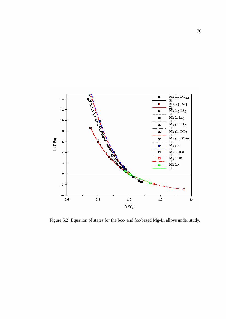
70
Figure 5.2: Equation of states for the bcc- and fcc-based Mg-Li alloys understudy.

71
bcc-structure Bulk Modulus (GPa)Calculated Experimental
Mg 37.57Mg15Li 32.94Mg3Li (DO3) 32.76
30.47[110]
65 at.% Mg 25.0[116]MgLi (B1) 16.74MgLi (B2) 22.11
20.25[110]
20.7[116]MgLi (B32) 25.25MgLi3 (DO3) 18.04
18.78[110] 15.0[116]MgLi15 23.12
Li 12.00 12.6[144]
[110] Calculated by exact muffin-tin orbitals (EMTO) method with GGA.[116] BCC phase at room temperature.
Table 5.4: The bulk moduli for bcc elemental Mg and Li as well as for bcc-basedMg-Li alloys

72
5.3 Heats of formation
The heat of formation is one of the prime thermodynamic ingredients in the free en-
ergy to determine phase diagrams, the other being entropy. Hence studying the rela-
tive stability of the different cubic-based superstructures, it is convenient to consider
the formation energy(Eform) of each structure. The formation energy is responsible
for the relative stability of the phases at low temperatures where entropic contribu-
tions are not important. The phase equilibria are determined by drawing thecommon
tangent [117] lines between the free energy curves of neighbouring compounds. The
heat of formation of the alloy Mg1−xLix is defined by
EMg1−xLixform = E
Mg1−xLixtotal − [xELi
solid + (1− x)EMgsolid] (5.3)
whereEMg1−xLixtotal is the total energy of the alloy,EMg
solid andELisolid are the total
energies of the stable structures of elemental Mg and Li, andx and(1 − x) refer to
the fractional concentrations of the constituent elements.
5.3.1 Li and Mg in hcp, fcc and bcc phases
The heats of formation (eq. 5.3) depend on finding the energies of the constituent
elements in their ground state structure. As can be seen from Table 5.5, our results
predict hcp Mg structure to be energetically favoured over the fcc andbcc structures,
consistent with experimental and other theoretical results [118, 119, 120]. For el-
emental Li, the situation is more complicated. The stable structure of Liis bcc at

73
temperatures above78◦K. Earlier work by Barrett [7] reported that at78◦K the hcp
phase coexists with the bcc phase, and that cold working at low temperatures pro-
duces the fcc phase at the expense of hcp and bcc phases, Li having undergone a
martensitic transformation. However, a later study [8] showed that the ground-state
structure of Li is neither hcp nor fcc, but a 9R-related complex close-packed struc-
ture suggested by Overhauser [9]. As shown in Table 5.5, our results found that
hcp Li is more stable than both fcc and bcc at zero temperature, although wedid
not compute 9R due to the large size of its unit cell. However, there is only avery
small energy difference between the phases, hcp being only0.06 meV more stable
than fcc. Since it is well known that the phases of Li are extremely close inen-
ergy [5, 121, 122, 123, 124, 125, 126], geometry optimizations had to be performed
with great caution. The smearing width is periodically halved during the planewave
pseudopotential calculation. We used0.01 and0.1 eV for minimum and maximum
smearing widths respectively, since values as low as0.01 eV have been previously
used to calculate the converged energy [25, 26]. However, we must stress that these
energy differences are so small that even a change in choice of exchange-correlation
functional can alter the predictions [121].
5.3.2 Fcc- and bcc-based ordered Mg-Li alloys
The calculated values of the heats of formation of the Mg-Li systems considered in
this study are summarized in Table 5.6, with asterisks denoting the predicted most

74
Equilibrium total energy Energy relative to hcpElement Phase E0 (eV/atom) (meV/atom)
This work Experiment[127]Mg hcp -977.892621 0.00 0.000
fcc -977.877264 15.36 27.04bcc -977.858844 33.78 32.27
Li hcp -190.029049 0.00 0.00fcc -190.028985 0.06 0.48bcc -190.027526 1.52 1.61
[127] Experimental thermodynamically based estimates using CALPHAD approach.
Table 5.5: Calculated equilibrium energies as well as energies relative to most stablephase, hcp, for pure elements (Mg and Li) in various phases. Experimental resultsare thermodynamic estimates within the CALPHAD approach.
75
stable phases amongst competing structures for a given stoichiometry. Figure 5.3
shows the plot of the heats of formation of the Mg-Li system versus composition.
We see that the curve takes a V-shape, with its minimum at the equi-concentration
MgLi compound. This is in agreement with the experimental heats of formation
of liquid Mg-Li alloys at 1000◦C [128] and the theoretical DFT results of Skriver
[110]. This excellent agreement between theory and experiment is fortuitous, since
the ordered structures should have heats of formation that are about30% lower in
energy than the corresponding enthalpies of formation of the disordered liquid state
[129].
At 50-50 concentration, the B2 structure is clearly seen as the most stable
phase, since it has the lowest formation energy amongst its competing counterparts
(Table 5.6). Our calculations predict that the B2 structure is lower by26 meV/atom
than that of B32. These results agree quantitatively with the earlier pseudopoten-
tial calculations by Hafner and Weber [112], and Hafner [31], who found B2 to be
lower in energy by116 meV/atom and88 meV/atom respectively. Our predicted
heat of formation for the B2 structure of−73.4meV/atom is in excellent agreement
with Skriver’s DFT result of−73.5 meV/atom [110]. Experimentally, a tendency
towards B2 (CsCl) type ordering has been observed at low temperatures[106, 107].
Interestingly, the difference in the calculated energy differenceof the L10 and B2
phases is small, which suggests that both phases might be present at very lowtem-
peratures, if only the kinetics were fast enough for phase transitions. We observed

76
Ordered structure Eform (meV/atom)This work Skriver[110] Experimental[128]
A15BMg15Li (bcc) 11.25A7BMg7Li -3.33A3BMg3Li (L12) -23.96 -21.2Mg3Li (DO22) -18.82 -20.7Mg3Li (DO3) -38.32* -48.7* -39.2ABMgLi (B2) -73.41* -73.5* -56.7MgLi (B32) -47.72MgLi (L10) c/a = 0.72 -72.01
c/a = 1 -44.16 -37.2AB3MgLi3 (L12) -36.61 -28.3MgLi3 (DO22) -37.43* -34.4MgLi3 (DO3) -31.12 -37.4* -31.0AB7MgLi7 -20.00AB15MgLi15 (bcc) -5.28
[110] Calculated by exact muffin-tin orbitals (EMTO) method with GGA.[128] Experiment for liquid alloys at 1000◦C.
Table 5.6: Heats of formation of Mg-Li alloys predicted by this work and by Skriver[109] for ordered structures compared to experimental values for liquid alloys at 1000degrees celsius [Mashovetz and Puchkov]. Asteriks denote the most stable phase atthat composition predicted by this work and Skriver [109].
a huge energy difference between our L10 result and Skriver’s. This was caused by
the fact that Skriver did not relax the c/a ratio so that his underlying lattice is truly
"fcc", hence MgLi (L10) becomes very unstable compared to B2, whilst ours was re-
laxed toc/a = 0.72. It became evident when we did a calculation with fixed ratio of
c/a = 1 that our result and Skriver’s were in reasonable agreement.
The heat of formation for Mg3Li in the three phases (Table 5.6) shows clearly
the preferred stability of the DO3 phase over the L12 and DO22 phases. The heat of

77
Figure 5.3: Predicted heats of formation for Mg-Li compounds compared with dis-ordered experimental results[128] . The common tangent construction for stabilitylimits of the different phases is indicated by the solid lines.

78
formation of Mg3Li in the L12 structure is higher by14.36 meV/atom compared to
the DO3 phase, with the DO22 phase being even bigger. Our predicted phase stabil-
ity ordering is the same as that of Skriver [110]. In the MgLi3 compound, the DO22
structure has the lowest formation energy with the L12 and DO3 phases lying only
0.82 and6.32 meV/atom higher, respectively. This slight difference between L12
and DO22 indicates a strong stability contest between these phases at this concen-
tration. We see that Skriver predicts the DO3 phase to be more stable than DO22.
However, this is probably because he did not relax the c/a axial ratio from its ideal
value of2.00. We found an equilibrium value of2.02 (Table 5.1).
In Figure 5.3, the solid common tangent lines are constructed for the stability
limits of the different phases. Among the structures considered, the most energeti-
cally favourable intermetallic phases at absolute zero are the DO3 Mg3Li, B2 MgLi,
DO22 MgLi 3 and MgLi7 compounds. The L12 and DO22 structures are metastable at
25% Li, while the B1, B32 and L10 structures are metastable at50% Li. Our equi-
librium calculations predict DO3 to be the most stable structure at A3B composition,
while at AB3 the DO22 structure shows more stability than its competitors.
The Mg-rich compounds, the bcc supercell Mg15Li and the fcc supercell Mg7Li,
lie well above the tangent line connecting hcp Mg (Eform= 0 eV ) with DO3 Mg3Li.
This clearly indicates the instability of the bcc and fcc Mg-Li compounds around
this region. This instability supports Hafner’s earlier work [31] that hcpMg-Li com-
pounds are dominant in the region with less than18% Li concentration. The for-

79
mation energy of Mg3Li in both the DO22 and L12 structures lie above tangent line,
which indicates the instability of the fcc lattice in this region. The energetically
favoured phase is DO3. Most of Mg-Li compounds at the Li-rich side lie either ex-
actly or very close to the line connecting B2 MgLi with elemental hcp Li. As far as
the stability is concerned in this region, fcc-based compounds are having an upper
hand over the bcc-based compounds. In both regions, our predicted stability pro-
file is in full agreement with Hafner’s earlier work [31] on disordered Li-Mg solid
solutions using second order perturbation theory.
5.4 Electronic density of states
Mg and Li are very good nearly-free-electron metals. This implies thattheir elec-
tronic properties can be understood by first considering those of a free electron
gas, in which the eigenvaluesE vary parabolically with the wave vectork asE =
(�2/2m)k2. Filling up these states with 2 electrons each following Pauli’s exclusion
principle, we arrive at the concept of the Fermi surface, which is spherical for a free
electron gas. As is well known, the corresponding density of statesn(E) of a free
electron gas varies as the square root of the energy.
The electronic densities of states (DOS) for the hcp, fcc and bcc phases of Mg
and Li are presented in Figure 5.4, using the CASTEP plane-wave methodology as
discussed in section 3.6. We have taken the Fermi levelEF as the zero energy. The
occupied part of the DOS for both Mg and Li in all three lattices show approximate

80
Figure 5.4: Density of states from CASTEP for elemental (a) Mg and (b) Li atoms inhcp, fcc and bcc lattices.
81
free-electron behaviour. This confirms that Mg and Li are good nearly-free electron
(NFE) metals since their occupied DOS are only a relatively small perturbation of
the free-electron density of states. However, we observe that Li, in all its three con-
sidered phases, displays very strong deviations from free-electron behaviourabove
the Fermi energy. This is a direct consequence of this first-row element havingno
p core electrons. This leads to large energy gaps opening up at the Brillouin zone
boundary, and hence large deviations from free-electron behaviour in the unoccupied
region of the DOS aboveEF .
The partial and total DOS for the Mg-Li ordered structures with respectto fcc-
and bcc-based lattices are shown in Figures 5.5-5.9. They agree with otherDFT cal-
culations in the literature [111, 114, 133]. We see that for all these different ordered
phases the occupied region of the total DOS is approximately free-electronlike. The
partial DOS reflects the primarily s-type bonding on the Li sites, but the hybridized
s-p bonding at the Mg sites, as expected for these monovalent and divalent metals,
respectively. Table 5.7 gives the calculated DOS at the Fermi level,n(EF ), for the
1:1 and 3:1 stoichiometries.
This relation between structural stability and the behaviour of the DOS in the
vicinity of the Fermi energy can be formalized by a Jones-type analysis [134]. Using
a rigid-band model, the theory shows how structure in the density of states translates
into an energy difference for competing phases as a function of the electron count.
Within the rigid-band approximation we assume that the bands of hcp, fcc, and bcc

82
Figure 5.5: The total density of states (DOS) and partial density of states(PDOS) forMgLi compound in (a) L10, (b) B2 and (c) B32 structures, respectively.

83
Figure 5.6: Total and partial density of states for Mg3Li composition in (a) L12, (b)DO3 and (c) DO22 structures.

84
Figure 5.7: Total and partial density of states for MgLi3 composition in (a) L12, (b)DO3 and (c) DO22 structures.

85
Figure 5.8: The total density of states (DOS) and partial density of states (PDOS) offcc-based superstructures, (a) Mg7Li and (b) MgLi7, respectively.

86
Figure 5.9: The total density of states (DOS) and partial density of states (PDOS) ofbcc-based superstructures, (a) Mg15Li and (b) MgLi15, respectively.

87
Compound Structure n(EF )(states/eV/atom)
Mg3Li L12 0.417DO22 0.312∗
DO3 0.367
MgLi B2 0.399∗
B32 0.445L10 0.412
MgLi3 L12 0.346∗
DO22 0.669DO3 0.564
Table 5.7: The total density of states at EF , n(EF ) (in states/eV per atom), of Mg3Liand MgLi3, in L12, DO22 and DO3 phases, and MgLi in B2, B32 and L10 phases,respectively. Asteriks denote the predicted stable phase.

88
lithium remain unchanged (or rigid) on alloying. A Jones analysis then statesthat the
structural energy difference between any two lattices at the same atomic volume is
given by
∆U = ∆Uband = ∆
[∫ EF
En(E)dE
], (5.4)
wheren(E) is the electronic density of states (DOS) per atom. The Fermi
energyEF is determined by the number of valence electrons per atom,N ≡ e/a,
according to
N =
∫ EF
n(E)dE. (5.5)
Jones showed that the energy difference equation (5.4) allows us to link the
relative stability of competing structures to the relative behaviourof the correspond-
ing DOS. To help us understand the behaviour of the bandstructure energy,∆Uband,
we exploit the following expressions for the first and second derivatives of∆Uband
(equation 5.4) with respect to the electron number,N , as follows:
d
dN(∆Uband) = ∆
[dEF
dNEFn(EF )
]= ∆EF , (5.6)
d2
dN2(∆Uband) = ∆
[1
n(EF )
], (5.7)
wheren(EF ) is the DOS at the Fermi energy for the electron numberN = e/a.
Taking the difference of equation (5.6) for two different structures, we see that the

89
derivative of the energy difference is zero at certain special band fillings for which
the two Fermi energies are equal. At these values ofN , the bandstructure energy
differance∆Uband is extremal or possibly (in rare cases) a saddlepoint. To identify
a maximum or a minimum, we take the difference of the inverses of their DOS at
EF , as given on the right-hand side of equation (5.7). If one of the structures has a
lower DOS at this Fermi level, an extremum is present and this structurehas a lower
energy.
We employed the ab initio TB-LMTO-ASA (tight-binding-linear muffin-tin or-
bitals within atomic sphere approximation) method [39, 135, 136] to calculate the
DOS for the hcp, fcc and bcc Li structures using the equilibrium cell parameters pre-
dicted by the CASTEP code (Section 4.4). To simulate the alloying with Mg, we
keep the Li band structures for hcp, fcc and bcc structures fixed and calculate the
bandstructure energies for an electron number varying between 0 and 2.
The difference of the bandstructure energies as a function of electron number
is shown in Figure 5.10, together with the Fermi energy difference and DOS, all
plotted againstN = e/a rather than energy. The top panel is the output quantity we
are interested in, namely the bandstructure energy difference. The hcp-fcc energy
difference curve has a minimum aroundN = 1.0 where the hcp DOS is lowest
and a maximum aroundN = 1.6 where the fcc DOS is lowest, whereas the hcp-
bcc curve has a minimum aroundN = 1.1 where the hcp DOS is lowest and a
maximum aroundN = 1.75 where the bcc DOS is lowest. The middle panel shows

90
the first derivative of the energy function, i.e. the Fermi energy difference ∆EF .
This quantity has a positive slope where the hcp DOS lies below both the fcc and bcc
DOS, and vice versa. The bottom panel presents the input, namely the DOS functions
for the different phases. The central point is that this gives essentiallythe second
derivative of∆Uband. Thus, where the bcc DOS lies above the fcc DOS, the curvature
of the energy difference function is such that the bcc structure will eventually become
more stable. We see that with increasing electron concentration, the sequence of
stable phases is hcp-fcc-bcc-hcp, in agreement with previous theoretical predictions
[31].
5.5 Elastic properties
From the perspective of materials physics, the elastic constantsCij contain some of
the more important information that can be obtained from ground-state total-energy
calculations. A given crystal structure cannot exist in a stable or metastable phase
unless its elastic constants obey certain relationships. TheCij also determines the
response of the crystal to external forces, as characterized by the bulkmodulus, shear
modulus, Young’s modulus, and Poisson’s ratio, and so play an important role in
determining the strength of a material [81]. First-principles calculations that use
periodic boundary conditions assume the existence of a single crystal, so all elastic
constants can be determined by direct computation. The calculatedCij can then be
used to check the experimental bulk and shear moduli, if available, and tocalibrate

91
0.0 0.5 1.0 1.5 2.0N
0.0
0.2
0.4
0.6
n(E
F)
(sta
tes
eV-1
ato
m-1
)
Li hcpLi fccLi bcc
-0.8
-0.6
-0.4
-0.2
0.0
0.2
∆ΕF (
eV)
-0.03
-0.01
0.01
0.03
0.05
0.07∆
Uba
nd (
eV a
tom
-1)
hcp - fcchcp - bcc
hcp-fcc
hcp-bcc
Figure 5.10: Energy difference, the Fermi energy difference and density of statesplotted against electron concentration. The plot begins atN = 0 so Li occurs in themiddle of the diagram whereN = 1 whilst Mg occurs whereN = 2.

92
model calculations. In addition, the elastic constants can be used to checkthe phase
stability of proposed compounds [137, 138]. First-principles calculations can thus
be used to predict the existence and properties of new materials and phases. In a
theoretical search for new materials, an interesting and important area of research is
to study binary compounds that exhibit high melting temperatures and large elastic
constants (which roughly correlate with "strength"). These alloys might begood
candidates for new structural materials, were they are not brittle [81].For a cubic
crystal to be mechanically stable it has to satisfy the following criterion:B = (C11+
2C12)/3 > 0, C ′ = (C11 − C12)/2 > 0, C44 > 0 at the equilibrium of the equation
of state, whereB andC ′ are the bulk and shear modulus, respectively.
We performed calculations of the elastic moduli of Mg-Li alloys using CASTEP
in Materials Studio version 3.0 [96]. Practical methods of determining theelastic co-
efficients from first principles usually set either the stress (or the strain) to a small
finite value, optimize any free parameters of the structure, and calculate the strain
(or stress). With a careful choice of the applied deformation, the elastic moduli can
then be determined. Applying a given homogeneous deformation (the strain) and
calculating the resulting stress requires far less computational effort,since the unit
cell is fixed and only the ionic positions require optimization. This is the method
implemented in the current work. The elastic properties were calculated by comput-
ing the components of the stress tensor for small strains using the method developed
by Nielsen and Martin [139]. For small strain, theC11andC12 elastic constants are

93
derived from the harmonic relationC11 = σ1/ǫ1 andC12 = σ2/ǫ1, whereσi and
ǫi represent respectively, the stress and the applied strain. The macroscopic stress
in the solid is computed for a small strain by the use of the stress theorem, and the
forces on the atoms are derived from the Hellman-Feynman theorem [102]. For an
ǫ4 strain (uniaxial strain in the(111) direction) there are internal displacements of
the sublattices, and the atomic positions in the unit cell are not determined only by
symmetry. Kleinmann [140] defines an internal strain parameterξ that describes the
displacements of the atoms.
The application of strain on the lattice implies a lowering of symmetryfrom
that of the crystal, therefore very accurate total-energy calculations are required since
the energy differences involved are of the order of10 to 1000 µeV/atom. This cir-
cumstance requires the use of a finek-point mesh. The calculations were considered
converged when the maximum force on atoms was below0.01 eV/A, the total en-
ergy change per atom was less than4x10−4 eV/atom and the displacement of atoms
was below4x10−4A. Both the energy and the stress were Pulay corrected to reduce
any remaining finite basis set errors. The calculations were done at ourtheoretically
determined (equilibrium) lattice constants for each structure, with aplane-wave ba-
sis set defined by an energy cut-off of500 eV for pure elements and400 eV for the
ordered superstructures, a very small smearing width of0.1 eV and sufficient sets
of k-points. These parameters are essential because the Fermi energy and hence the
total energy depend quite sensitively on them.

94
For each of the structures, six different values of the strain±0.0008, ±0.0024
and±0.004were used. The value of the stress is calculated for each strain. A linear fit
of the stress-strain relationship for each component of the stress is computed and its
gradient provides the value of the elastic constant. With our choice of special k-points
in the full Brillouin zone and cut-off energy, the energy per atom was converged
to 0.1 meV/atom and4 meV/atom or less for pure elements and superstructures,
respectively.
The calculated elastic constants for the Mg-Li systems are compared toavail-
able experimental data and the results of other calculations in Table 5.8. We find that
the elastic constants of pure Mg in the hcp phase are in acceptable agreement with
experimental results [130] as well as previous theoretical results [141] with the ex-
ception ofC44 which is about50% too small. The elastic constants of the fcc lattice
Mg are also in good agreement with the available theoretical results while the bcc
phase is found to be mechanically unstable, since the tetragonal shear modulusC ′ is
negative. Our results for pure Li show mechanical stability in all threephases with
the elastic constants being in good agreement with both experimental [143] and pre-
vious theoretical results [81, 141], except for the case ofC11 andC44 of the bcc
lattice which are overestimated.
Our calculated elastic constants for tetragonal systems show a smallvalue of
C44 in comparison toC66, which means that the tetragonal unit cell is more easily
deformed by a pure shear abouta andb axes in comparison to thec axis, with the

95
Composition Structure C11 C12 C44 C13 C33 C66 B V0d2EdV 2
GPa GPa GPa GPa GPa GPa GPa GPaMg This work hcp 59.84 24.25 8.31 16.09 70.56 17.80 33.67Calculated[141] hcp 66.20 22.10 18.00 16.60 62.50 22.05 33.94Experiment[130] hcp 63.48 25.94 18.42 21.70 66.45 18.77 35.40Mg This work fcc 42.75 30.96 23.09 - - - 34.89 34.11Calculation[142] fcc 46.00 27.40 30.00 - - - 33.60Mg This work bcc 25.65 39.41 35.96 - - - 34.82 37.57Mg15Li This work bcc 55.77 24.70 50.93 - - - 35.06 32.94Mg7Li This work fcc 22.21 29.47 24.23 - - - 27.05 33.99Mg3Li This work L12 25.78 29.93 24.50 - - - 28.54 27.15Calculated[110] 29.45
DO22 24.30 28.17 30.44 27.64 23.63 31.13 26.60 28.03Calculated[110] 28.87
DO3 39.96 25.59 41.03 - - - 30.38 32.76Calculated[110] 30.47MgLi B2 37.51 19.70 25.91 - - - 25.64 22.11Calculated[110] 20.25Exp.[128] 55% Mg B2 32.20 19.80 26.60 - - - 23.90Exp.[128] 45% Mg B2 28.50 20.50 19.40 - - - 23.20
B32 30.99 24.55 28.55 - - - 26.70 25.25L10 53.66 1.37 33.57 19.95 31.18 10.98 24.47 25.25
Calculated[110] 24.17MgLi3 This work L12 25.76 15.94 18.68 - - - 19.21 19.07Calculated[110] 18.76
DO22 28.86 13.86 21.66 14.49 27.37 23.27 18.97 17.49Calculated[110] 18.84
DO3 19.42 17.79 15.42 - - - 18.33 18.04Calculated[110] 18.78MgLi7 This work fcc 15.83 16.95 11.70 - 16.58 16.42MgLi15 This work bcc 18.24 13.25 11.52 - - - 14.92 23.12Li This work hcp 24.34 4.76 6.37 4.54 24.86 9.79 11.25Li This work fcc 17.51 11.42 9.31 - - - 13.45 13.92Calculated[81] fcc 14.10 7.80 8.60 - - - 9.90Li This work bcc 19.65 10.93 16.12 - - - 13.84 12.00Calculated[141] bcc 13.00 11.00 11.40 - - - 11.60Calculated[81] bcc 15.60 14.80 11.20 - - - 10.60Experiment[143] bcc 14.50 12.10 11.60 - - - 13.00Experiment[144] bcc 13.50 11.40 8.80 - - - 12.10
Table 5.8: Calculated elastic properties of Mg-Li alloys at equilibrium lattice para-meters. The bulk moduli determined from elastic constants is compared with theones calculated from equation of states.

96
Composition Structure C′ B/C′ E ν AGPa GPa
Mg This work hcp 15.80 2.13 64.41 0.19 A1 = 1.00A2 = 0.34
Calculated[141] hcp 20.92 1.62 56.26 0.19 -Experiment[130] hcp - - 45.00 0.35 -Mg This work fcc 5.89 5.92 16.75 0.42 3.92Calculation[142] fcc 9.30 3.61 25.54 0.37 3.23Mg This work bcc -6.88 5.06 -22.09 0.61 -5.23Mg15Li This work bcc 15.54 2.26 40.60 0.31 3.28Mg7Li This work fcc -3.63 7.45 -11.41 0.57 -6.28Mg3Li This work L12 -2.08 13.72 -6.38 0.54 -11.81
DO22 17.65 1.51 -5.50 0.53 A1 = −16.09A2 = −16.57
DO3 7.19 4.23 19.97 0.39 5.71MgLi This work B2 8.91 2.88 23.94 0.34 2.91Experiment[128] 55% Mg B2 8.33 - 17.12 0.38 4.29Experiment[128] 45% Mg B2 5.44 - 11.35 0.42 4.85
B32 3.22 8.29 9.30 0.44 8.87L10 22.11 1.11 16.71 0.36 A1 = 0.42
A2 = 2.99MgLi3 This work L12 4.91 3.91 13.58 0.38 3.80
DO22 16.13 1.18 17.54 0.34 A1 = 3.10A2 = 3.18
DO3 0.82 22.35 2.42 0.48 18.92MgLi7 This work fcc -0.56 29.60 -1.70 0.52 -20.89MgLi15 This work bcc 2.50 5.97 7.09 0.42 4.62Li This work hcp 2.32 4.85 23.44 0.16 A1 = 1.00
A2 = 0.63Li This work fcc 3.05 4.42 8.49 0.39 3.06Calculated[81] fcc 5.80 1.71 14.00 0.35 2.73Li This work bcc 4.36 3.17 11.83 0.36 3.70Calculated[141] bcc 1.00 11.60 2.91 0.46 11.40Calculated[81] bcc 3.40 3.12 9.30 0.40 16.70Experiment[144] bcc 3.90 3.10 10.50 0.36 8.38
Table 5.9: Other derived elastic moduli of Mg-Li alloys, namely shear modulus (C’),the ratio of bulk modulus to shear modulus (B/C’), Young’s modulus (E), Poisson’sratio (v) and the shear anisotropy factor (A).

97
exception of L10 structure wherein the opposite is the case. The smallC44 value
indicates that Mg-Li alloys are marginally stable with respect to the〈010〉 shear on
the(010) plane in this region.
In Table 5.9, we list the values ofB/C ′ of Mg-Li alloys together with their
shear modulus(C ′), Young’s modulus(E), Poisson’s ratio (ν) and shear anisotropy
factor(A). The bulk moduli decrease monotonically with the addition of Li content.
The bulk moduli obtained from elastic constants agrees well with the experimental
and other previous theoretical results including the ones extracted from equation of
states. TheB/C ′ values of 1.11, 1.18 and 1.51 for MgLi (L10), MgLi3 (DO22) and
Mg3Li (DO22) , respectively, suggest that these compounds to be brittle, while the
remaining ones appear to be ductile since their values are above the critical value of
1.75. The values ofB/C ′ for all our Mg-Li systems, except for compounds listed
above, are generally larger than those of pure elements, Mg and Li. It isalso inter-
esting to note that cubic Mg3Li (DO3) structure is the only phase that is stable at this
concentration and has a positive value of Young’s modulusE. For most of our struc-
tures, the derivedν is slightly higher than the isotropic value of13, thus resulting to
E being less thanB. We also observed that an increase in Li content increases the
Poisson ratio as well as the anisotropy.
The elastic constants of our cubic Mg-Li systems listed in Table 5.8 obey the
stability conditions as outlined in Section 4.4, including the fact thatC12 must be
smaller thanC11, except for Mg bcc, Mg7Li, Mg3Li (L1 2) and MgLi7 structures. The

98
conditions also lead to a restriction on the magnitude ofB. SinceB is a weighed
average ofC11 andC12 and stability requires thatC12 be smaller thanC11, we are
then left with the result thatB is required to be intermediate in value betweenC11
andC12,
C12 < B < C11.
The elastic constants in Table 5.8 for tetragonal phases, L10 and DO22 strucutres,
satisfy all of the above conditions. In particular,C12 is smaller thanC11 andC13 is
smaller than the average ofC11 andC33. The only structure that does not satisfy these
stability restrictions is Mg3Li in DO22 phase, thus showing mechanical instability.
Figure 5.11 presents in (a) the tetragonal shear modulusC ′ of our ordered bcc-
and fcc-based superstructures and (b) the predicted energy differencebetween the
corresponding bcc and fcc ordered compounds relative to hcp Mg and Li lattices,
both plotted against the electron per atom ratio ranging from 1 (Li) to 2 (Mg). We
find an interesting correlation between these quantities, that, in the region where bcc
is very stable compared to fcc, the shear modulus is positive for bcc but negative
for fcc (i.e. the fcc lattice is the mechanically unstable) and vice versa. The similar
behaviour had been pointed out earlier for elemental transition metals by Craievich et
al [145] and B2 and L10 TiAl by Sob et al [146]. This reflects the underlying change
in hcp to fcc to bcc to hcp structural stability as the electron per atom ratio changes
from 1 (Li) to 2 (Mg).

99
Figure 5.11: Plot of (a) tetragonal shear modulusC ′of ordered bcc- and fcc-basedMg-Li superstructures and (b) the relative formation energies of the correspondingbcc and fcc Mg-Li compounds, against the electron per atom ratio.

100
Chapter 6CONCLUSION AND FUTURE WORK
6.1 Conclusion
The first principles pseudopotential calculations based on the generalizedgradient
approximation (GGA) within density functional theory (DFT) have been utilized to
succesfully investigate the cohesive, electronic and elastic properties of cubic-based
Mg-Li alloys. In addition to calculating all of the equilibrium structural parame-
ters (Sec. 5.1-5.4) we have also obtained values for all of the zero-pressureelastic
constants (Sec. 5.5) for the Mg-Li compounds considered in this study.
We found that with increasing Li composition the volume shrinks and some
kind of a parabolic or V-shaped trend with minimum at the equiatomic composition
was observed in both fcc and bcc structures. This behaviour is clearly shown in
Figure 5.1, wherein, Vegard’s law [108] or Zen’s law [115] , which assumes a linear
dependence of the lattice constants or mean atomic volumes, respectively,of solid
solutions with composition (as shown in Fig. 5.1 by solid lines), is directly violated
in both fcc- and bcc-based superstructures as expected and this was also observed
in earlier experiments [106] as well as previous theoretical investigations [31]. The
trend of decrease in the Mg-rich region until50 atomic per cent solute, at which the

101
behaviour is slowly reversed in the Li-rich region, of the lattice constant with the
addition of Li for bcc structures was also obtained from earlier experiments [106].
Our results predict hcp Mg structure to be energetically favoured over the
fcc and bcc structures, consistent with experimental and other theoretical results
[118, 119, 120]. Our results showed that hcp Li is more stable than both fcc and bcc
at zero temperature, agreeing with the experiment [7], but with only a very small en-
ergy difference (especially between fcc and hcp). Since it is known that these phases
(Li) are close in energy [5, 122, 121, 123, 124, 125, 126], geometry optimizations
had to be performed with great caution. As a function of concentration, the heats
of formation plot shows a V-shape curve, with a minimum at the equi-concentration
MgLi compound, which is in agreement with the experimental work [128] and pre-
vious theoretical results [141]. The predicted heats of formation for all the different
ground state superstructures result in a representative stability profile, which shows
that the DO3, B2 and DO22 structures are the most stable amongst various phases hav-
ing Mg3Li, MgLi and MgLi3 compositions, respectively. In both regions (Mg-rich
and Li rich sides), our predicted stability profile is in full agreement with Hafner’s
earlier work [31] on disordered Li-Mg solid solutions.
The general trend in the total DOS is that from the bottom of the valence band
the DOS increases smoothly as a function of energy as they would in a free-electron
system up toEF or just slightly above it. The Jones-analysis method compliments the

102
heats of formation, DOS and elastic constants results in that the predicted structural
stability profile is hcp-fcc-bcc-fcc, in agreement with previous results of Hafner [31].
The bulk moduli decrease monotonically with the addition of Li content. The
equation of state bulk moduli is in good agreement with both the experimental[116]
and other previous theoretical [110] results. TheB/C ′ values of 1.11, 1.18 and
1.51 for MgLi (L10), MgLi3 (DO22) and Mg3Li (DO22) respectively, suggest that
these compounds to be brittle, while the remaining ones appear to be ductile since
their values are above the critical value of 1.75. These following structures, Mg
bcc, Mg7Li, Mg3Li (L1 2), Mg3Li (DO22) and MgLi7 were found to be mechanically
unstable. We also observed that an increase in Li content increases the Poisson ratio
as well as the anisotropy.
6.2 Future work and recommendations
The predicted heats of formation with respect to different underlying lattices such as
fcc or bcc will be used as an essential input for calculating effective cluster interac-
tions, from which theoretical phase diagrams can be computed using Monte Carlo
[19] or the Cluster Variation Method (CVM) [20].
The elastic moduli calculated here, in particular, Young’s modulus and Poisson
ratio, will serve as an input to an object oriented finite (OOF) [147] element program.
This program (OOF) will be used on the micrographs (pixels) of Mg-Li samples ob-
tained from the electron microscope (EM) to initiate microstructuralstudies of these

103
alloys. These includes simulations of stress distributions and predictionsof mechan-
ical behaviour (evolution with temperature, pressure and composition) of alloys and
fracture processes.
This work will form the basis for future study in collaboration with the CSIR
on the strengthening of Mg-Li alloys by the addition of ternary elements.

104
REFERENCES
[1] J.H. Jackson, P.D. Frost, A.C. Loonam, L.W. Eastwood, and C.H. Lorig,Trans. AIME,185, 149 (1948).
[2] S.S. Rajput, R. Prasad and R.M. Singru, J. Phys. Condens. Mat.,5, 6419(1993).
[3] B.L. Mordike and T. Ebert, Mat. Sci. and Eng. A,302, 37 (2001).
[4] A.A. Nayeb-Hashemi , J.B. Clark and A.D. Pelton, Bull. Alloy Phase Dia-grams,5, 365 (1984).
[5] P. Staikov, A. Kara and T.S. Rahman, J. Phys.: Condens. Matter,9, 2135(1997).
[6] C.S. Barrett, Phys. Rev.,72, no. 3, 245 (1947).
[7] C.S. Barrett, Acta Cryst.,9, 671 (1956).
[8] C.M. McCarthy, C.W. Thompson and S.A. Werner, Phys. Rev. B,22, 574(1980).
[9] A.W. Overhauser, Phys. Rev. Lett.,53, 64 (1984).
[10] H.G. Smith, Phys. Rev. Lett.,58, 1228 (1987).
[11] W. Schwarz and O. Blaschko, Phys. Rev. Lett.,65, 3144 (1990).
[12] Polmer I.J. (1989), Light alloys-Metallurgy of the light metals (NewYork:Chapmann and Hall, Inc).
[13] S. Schumann and H. Friedrich, The Use of Mg in Cars-Today and in Future,Conference paper at Mg Alloys and their applications, 23-30/04/98, Wolf-burg, Germany.
[14] C.R. Chakravorty, Bull. Mater. Sci., Vol. 17, No. 6, November 1994, pp 733-745.

105
[15] Frost P.D. (1965), NASA-SP-5028 (Washington DC: NASA).
[16] A. Cottrell, Mater. Sci. Tech.,5, 1165 (1989).
[17] A. Kelly, W.R. Tyson and A.H. Cottrell, Phil. Mag.,15, 567 (1967).
[18] J.M. Sanchez, F. Ducastelle and D. Gratias, Physica128A, 334 (1984).
[19] K. Binder, in Monte Carlo Methods in Statistical Physics, Vol. 7 ofTopics inCurrent Physics, edited by K. Binder (Springler, Berlin, 1986), p. 1.
[20] R. Kikuchi, Phys. Rev.81, 988 (1951).
[21] G.P. Das, A. Arya and S. Banerjee, Intermetallics,4, 625 (1996) and refer-ences therein.
[22] S.H. Wei, L.G. Ferreira, and A. Zunger, Phys. Rev. B,45, 2533 (1992).
[23] Z. Shi, M. Lin, D. Naik and J.L. Gole, J. Power Sources,92, 70 (2001).
[24] H. Haferkamp, W. bach and P. Juchmann, New Magnesium-Lithium alloysof higher ductility.
[25] M.C. Payne, M.P. Teter, D.C. Allan, T.A. Ariar and J.D. Joannopoulos, Rev.Mod. Phys.,64, 1045 (1992).
[26] V. Milman, B. Winkler, J.A. White, C.J. Pickard, M.C. Payne, E.V. Akhmatskayaand R.H. Nobes, Int. J. Quantum Chem.77, 895 (2000).
[27] P.C. Hohenberg and W. Kohn, Phys. Rev. B,136, 864 (1964).
[28] A. Jayaraman, Rev. Mod. Phys.,55, 65 (1983).
[29] E. Wimmer, Computational Methods for Atomistic Simulations of Materials,
http://www.accelrys.com/technology/qm/erich/choices/html.
[30] J.A. Majewski and P. Vogl, Chapter IV in The Structure of BinaryCom-pounds edited by F.R. de Boer and D.G. Pettifor, Elsevier Science PublishersB.V., 1989.

106
[31] J. Hafner, J. Phys. F,6, 1243 (1976).
[32] J.C. Phillips, Phys. Rev.,112, 685 (1958).
[33] M.L. Cohen and V. Heine, Solid State Physics,24, 37 (1970).
[34] J.C. Slater, Phys. Rev.,51, 846 (1937).
[35] J.C. Slater, Quantum Theory of Molecules and Solids, Volume4, The self-consistent field for molecules and solids, McGraw-Hill, New York (1974).
[36] J. Korringa, Physica,13, 392 (1947).
[37] W. Kohn and N. Rostoker, Phys. Rev.,94, 1111 (1954).
[38] D.D. Koelling and G.O. Arbman, J. Phys. F,5, 2041 (1975).
[39] O.K. Andersen, Phys. Rev. B,12, 3060 (1975).
[40] E. Wimmer, H. Krakauer and A.J. Freeman, Electronics and ElectronPhysics,ed. by P.W. Hawkes, Vol.65, p. 357, Academic Press, Orlando (1985) andreferences therein.
[41] G.B. Bachelet, D.R. Hamann and M. Schluter, Phys. Rev. B,26, 4199 (1982).
[42] R. Car and M. Parrinello, Phys. Rev. Lett.,55, 2471 (1985).
[43] J.P. Perdew and Wang Yue, Phys. Rev. B,33, 8800 (1986).
[44] J. Labanowski and J. Andzelm, editors, Density Functional Methods in Chem-istry, Springler-Verlag, New York, (1991).
[45] J.C. Slater and G.F. Koster, Phys. Rev.,94, 1498 (1954).
[46] I. Lefebvre, M.Lannoo, and G. Allan, Phys. Rev. B,39, 13518 (1989).
[47] C. Mottet, G. Tréglia, and B. Legrand, Phys. Rev. B,46, 16018 (1992).
[48] E. Salomons, P. Bellon, F. Soisson, and G. Martin, Phys. Rev. B,45, 4582(1992).

107
[49] R. Haydock, V. Heine, and P. J. Kelly, J. Phys. C,5, 2845 (1972),8, 2591(1975).
[50] P. Turchi and F. Ducastelle, The Recursion Method and Its Applications,D.G. Pettifor and D. L. Weaire, editors, Springer-Verlag, Berlin p. 104 (1985).
[51] M. Aoki, Phys. Rev. Lett.,71, 3842 (1993).
[52] D.G. Pettifor, Phys. Rev. Lett.,63, 2480 (1989).
[53] D.R. Bowler, M. Aoki, C.M. Goringe, A.P. Horsfield and D.G. Pettifor,Mod-elling Simul. Mater. Sci. Eng.,5, 199 (1997).
[54] S. Znam, D. Nguyen-Manh, D.G. Pettifor and V. Vitek, Phil. Mag.,83, 415(2003).
[55] D.R. Hartree, Proc. Camb. Phil. Soc.,24, 89 (1928).
[56] V. Fock, Z. Phys.,61, 126 (1930) and ibid62, 795 (1930).
[57] C. Møller and M.S. Plesset, Phys. Rev.,46, 618 (1934).
[58] A.V. Krasheninnikov, Lectures on Introduction to electronic structurecalcu-lations,
www.acclab.helsinki.fi/~akrashen/esctmp.html.
[59] L.H. Thomas, Proc. Camb. Phil. Soc.,23, 542 (1927).
[60] E. Fermi, Z. Physik,48, 73 (1928).
[61] J. Kohanoff and N.I. Gidopoulos, Density Functional Theory: Basics, NewTrends and Applications Vol. 2, Part 5, Chapter 26, pp 532, in Hanbbookof Molecular Physics and Quantum Chemistry, John Wiley & Sons, Ltd,Chichester, 2003.
[62] M. Born and R. Oppenheimer, Ann. Physik,84, 457 (1927).
[63] W. Kohn and L.J. Sham, Phys. Rev. A,140, 1133 (1965).
[64] F. Bloch, Z. Physik,57, 545 (1929).

108
[65] J. Hafner, Acta Mater,48, 71-92 (2000).
[66] J.P. Perdew, J.A. Chevary, S.H. Vosko, K.A. Jackson, D.J. Singh and C. Fi-olhais, Phys. Rev. B,46, 6671 (1992).
[67] E. Hult, Y. Andersson and B.I. Lundqvist, Phys. Rev. Lett.,77, 2029 (1996).
[68] W. Kohn, Y. Meir and D.E. Makarov, Phys. Rev. Lett.,80, 4153 (1998).
[69] J.P. Perdew, Phys. Rev. B,33, 8822 (1986).
[70] A.D. Becke, Phys. Rev. A,38, 3098 (1988).
[71] J.P. Perdew and Y. Wang, Phys. Rev. B,45, 13244 (1992).
[72] J.P. Perdew, K. Burke and M. Ernzerhof, Phys. Rev. Lett.,77, 3865 (1996).
[73] G. Kresse, J. Furthmüller and J. Hafner, Phys. Rev. B,50, 13181 (1994).
[74] T.C. Leung, T.C. Chan and B.N. Harmon, Phys. Rev. B,44, 2923 (1991).
[75] T. Asada and K. Terakura, Phys. Rev. B, 47, 15992 (1993).
[76] J.P. Perdew and A. Zunger, Phys. Rev. B,23, 5048 (1981).
[77] D.M. Ceperly and B.J. Alder, Phys. Rev. Lett.,45, 566 (1980).
[78] J.P. Perdew, K. Burke and M. Ernzerhof, Phys. Rev. Lett.78, 1396 (E)(1997).
[79] E.H. Lieb and S. Oxford, Int. J. Quantum Chem.,19, 427 (1981).
[80] P. Ravindran, L. Fast, P.A. Korzhavyi, B. Johansson, J. Willis and O. Eriks-son, J. App. Phys.84, 4891 (1998).
[81] M.J. Mehl, B.M. Klein, and D.A. Papaconstantopoulos, Intermetallic Com-pounds: Vol. 1, Principles. Edited by J.H. Westbrook and R.L. Fleischer,1994, John Wiley & Sons Ltd.
[82] N.W. Ashcroft and N.D. Mermin, Solid State Physics, Saunders College,Philadelphia (1976).

109
[83] M.J. Mehl, Phys. Rev. B,61, 1654 (2000).
[84] J.F. Nye, Physical Properties of Crystals, Clarendon, Oxford (1957).
[85] D.C. Wallace, Thermodynamics of Crystals (Wiley, New York, 1972), Chap-ter 1.
[86] D. Iotova, N. Kioussis and S.P. Lim, Phys. Rev. B,54, 14413 (1996).
[87] S.F. Pugh, Philos. Mag.45, 823 (1954).
[88] W. Koster and H. Franz, Metall. Rev.,6, 1 (1961).
[89] M.H. Ledbetter, Materials at Low Temperatures, edited by R.P. Reed andA.F. Clark, p. 1.
[90] W.A. Harrison, Electronic Structure and the Properties of Solids, editedbyFreeman, San Francisco (1980).
[91] M.J. Gillan, Computer Simulation in Materials Science , edited by M. Meyerand V. Poutikis (Dordrecht: Kluwer) p. 257 (1991).
[92] N. Troullier and J.L. Martins, Phys. Rev. B,43, 1993 (1991).
[93] J.S. Lin, A. Qteish, M.C. Payne and V. Heine, Phys. Rev. B,47, 4174 (1993).
[94] A.M. Rappe and J.D. Joannopoulos, Computer Simulation in Materials Sci-ence ed M. Meyer and V. Poutikis (Dordrecht: Kluwer) p. 409 (1991).
[95] D. Vanderbilt, Phys. Rev. B,41, 7892 (1990).
[96] M.D. Segall, P.L.D. Lindan, M.J. Probert, C.J. Pickard, P.J. Hasnip, S.J.Clark and M.C. Payne, J. Phys. Cond. Matt.,14, 2717 (2002).
[97] F. Wagner, Th. Laloyaux and M. Scheffler, Phys. Rev. B,57, 2102 (1998).
[98] M.J. Gillan, J. Phys.: Condens. Matter1, 689 (1989).
[99] Grotheer and Fähnle, Phys. Rev. B,58, 13459 (1998).
110
[100] Y. Mishin, D. Farkas, M.J. Mehl and D.A. Papaconstantopoulos, Phys. Rev.B, 59, 3393 (1999).
[101] O. Le Bacq, F. Willaime and A. Pasturel, Phys. Rev. B,59, 8508 (1999).
[102] H. Hellmann, Einfukrung in die Quantumchemie (Deuticke, Leipzzig,1937),pp. 61 and 285; R.P. Feynman, Phys. Rev.,56, 340 (1939).
[103] P. Pulay, Molec. Phys.,17, 197 (1969).
[104] H.J. Monkhorst and J.D. Pack, Phys. Rev. B,13, 5188 (1976).
[105] W. Pitsch, in Phase Stability in High Temperature Alloys, edited by V. Guttmann(Applied Science Publishers, London, 1981), p. 1.
[106] D.W. Levinson, Acta Met.,3, 294 (1955).
[107] F.H. Herbstein and B.L. Averbach, Acta Met.,4, 407 (1956).
[108] L. Vegard, Z. Phys.,5, 17 (1921).
[109] V.G. Vaks and A.V. Trefilov, J. Phys. F: Met. Phys.,18, 213 (1998).
[110] H.L. Skriver, Materials Science Databases, CAMP, DTU, http://databases.fysik.dtu.dk/.
[111] B.R. Sahu, Mat. Sci. Eng. B,49, 74 (1997).
[112] J. Hafner and W. Weber, Phys. Rev. B,33, 747 (1986).
[113] S.H. Kellington, D. Loveridge and J.M. Titman, Brit. J. Appl. Phys. (J. Phys.D), Ser. 2, Vol. 2, 1162 (1969).
[114] R. Laihia, K. Kokko, K. Mansikka and P.T. Salo, J. Phys. C,6, 10247 (1994).
[115] E-an Zen, Am. Mineral,4, 523 (1956).
[116] R.W. Lynch and L.R. Edwards, J. Appl. Phys.,41, 5135 (1970).
[117] A. Cottrell, An Introduction to Metallurgy, Second Edition ,1975.
111
[118] L. Kaufman and H. Bernstein, Computer Calculation of Phase Diagrams(Academic, New York, 1970).
[119] A.K. McMahan and J.A. Moriarty, Phys. Rev. B,27, 3235 (1983).
[120] H.J. Gotsis, D.A. Papaconstantopoulos and M.J. Mehl, Phys. Rev. B,65,134101 (2002).
[121] K. Doll, N.M. Harrison and V.R. Saunders, J. Phys.: Condens. Matter,11,5007 (1999).
[122] M.M. Dacorogna and M.L. Cohen, Phys. Rev. B,34, 4996 (1986).
[123] J.A. Nobel, S.B. Trickey, P. Blaha and K. Schwarz, Phys. Rev. B,45, 5012(1992).
[124] J.C. Boettger and R.C. Albers, Phys. Rev. B,39, 3010 (1989).
[125] A.Y. Liu, A.A. Quong, J.K. Freericks, E.J. Nicol and E.C. Jones, Phys. Rev.B, 59, 4028 (1999).
[126] H. Bross and R. Stryczek, Phys. Status Solidi B,144, 675 (1987).
[127] N. Saunders, A.P. Miodownik and A.T. Dinsdale, CALPHAD,21, 351 (1988).
[128] V.P. Mashovetz and L.V. Puchkov, Zh. Prikl. Chem., 1875 (1965).
[129] F. Ducastelle, Order and phase stability in alloys Vol. 3, 1991, Elsevier(Netherlands).
[130] C. Kittel, Introduction to Solid State Physics, 7th Edition, 1996, John Wiley& Sons, Inc., New York.
[131] D.G. Pettifor, Bonding and Structure of Molecules and Solids, Oxford Uni-versity Press Inc., New York (1996).
[132] J. -H. Xu, T. Oguchi and A.J. Freeman, Phys. Rev. B,35, 6940 (1987).
[133] I.A. Abrikosov, Yu.H. Vekilov, P.A. Korzhavyi, A.V. Ruban and L.E. Shilkrot,Solid State Comm.83, 867 (1992).

112
[134] H. Jones, Proc. Phys. Soc. A,49, 250 (1937).
[135] O.K. Andersen, O. Jepsen and M. Sob, Electron Band Structure and its Ap-plications, edited by M. Yossouff, Springer-Verlag, Berlin, 1987.
[136] H.L. Skriver, The LMTO method (Springer-Verlag, Berlin, 1984).
[137] J. Chen, L.L. Boyer, H. Krakauer, and M.J. Mehl, Phys. Rev. B, 37, 3295(1988).
[138] M.J. Mehl and L.L. Boyer, Phys. Rev. B, 43, 9498 (1991).
[139] O.H. Nielsen and R.M. Martin, Phys. Rev. B,32, 3780 (1985),32, 3792(1985).
[140] L. Kleinman, Phys. Rev., 128, 2614 (1962).
[141] P. Beauchamp, R. Taylor and V. Vitek, J. Phys. F. Metal Phys.5, 2017 (1975).
[142] A. Zhu, B.M. Gable, G.T. Shiflet and E.A. Starke Jr., Acta Mater.52, 3671(2004).
[143] R. A. Felice, J. Trivisonno, D. E. Schuele, Phys. Rev. B,16, 5173 (1977).
[144] G. Simmons and H. Wang, Single Crystal Elastic Constants and CalculatedAggregate Properties: A handbook, 2nd ed. (MIT Press, Cambridge, Massa-chusetts, 1971).
[145] P.J. Craievich, M. Weinert, J.M. Sanchez and R.E. Watson, Phys. Rev. Lett.,72, 3076 (1994).
[146] M. Sob, L.G. Wang and V. Vitek, Comp. Mat. Sci.,8, 100 (1997).
[147] S.A. Langer, W.C. Carter and E.R. Fuller Jr.,OOF, NIST, Gaithersburg, MD,1997.
[148] X.Q. Guo, R. Podloucky and A.J. Freeman, Phys. Rev. B,42, 10912 (1990).

113
Appendix APapers presented at Local andInternational Conferences
Oral Presentations
1. Cohesive, electronic and elastic properties of cubic-based Mg-Li alloys, 7th
Annual Materials Modelling Meeting (MMM), 2004, University of the North,
Sovenga, SA.
2. Cohesive and elastic properties of ordered cubic-based Mg-Li alloys,
48th South African Institute of Physics (SAIP) Annual Conference, 2003,
University of Stellenbosch, Stellenbosch, SA.
3. A computational study of structural, electronic and elastic propertiesof
cubic-based Mg-Li alloys, 5th and 6th Annual MMM 2002-3, University of the
North, Sovenga, SA.
4. Ab initio study structural, electronic and elastic properties ordered cubic-
based Mg-Li alloys, 47th SAIP Annual Conference, 2002, Potchefstroom
University, Potchefstroom, SA.
5. Ab initio study of structural, electronic and elastic properties of cubic-based
Mg-Li alloys, Unin Post-graduate Society, 2002, University of the North,
Sovenga, SA.
6. Cohesive, Electronic and Elastic Properties of ordered Mg-Li alloys,

114
Royal Society-National Research Foundation Programme, 2004, Pretoria, SA.
Posters Presentations
1. Structural and Electronic properties of ordered Mg-Li compounds, 49th South
African Institute of Physics (SAIP) Annual Conference, 2004, University of
Free-State, Free-State, SA.
2. Cohesive properties of cubic-based Mg-Li alloys, CCP5 Summer School
2003, King’s College, London, UK.
3. A study of structural properties of Mg-Li alloys, 46th SAIP Annual
Conference, University of Natal, Durban, 2001, SA.
4. A study of structural properties of Al-Cu alloys, 4th Annual MMM 2001,
University of the North, Sovenga, SA.