Ab initio calculations of the isotopic dependence of nuclear clustering

Serdar Elhatisari,1, 2 Evgeny Epelbaum,3, 4 Hermann Krebs,3, 4 Timo A. Lahde,5

Dean Lee,6, 7, 4 Ning Li∗,5 Bing-nan Lu†,5 Ulf-G. Meißner,1, 5, 8 and Gautam Rupak9

1Helmholtz-Institut fur Strahlen- und Kernphysik and Bethe Center for Theoretical Physics, Universitat Bonn, D-53115 Bonn, Germany2Department of Physics, Karamanoglu Mehmetbey University, Karaman 70100, Turkey

3Institut fur Theoretische Physik II, Ruhr-Universitat Bochum, D-44870 Bochum, Germany4Kavli Institute for Theoretical Physics, University of California, Santa Barbara, CA 93106-4030, USA

5Institute for Advanced Simulation, Institut fur Kernphysik,and Julich Center for Hadron Physics, Forschungszentrum Julich, D-52425 Julich, Germany6National Superconducting Cyclotron Laboratory, Michigan State University, MI 48824, USA

7Department of Physics, North Carolina State University, Raleigh, NC 27695, USA8JARA - High Performance Computing, Forschungszentrum Julich, D-52425 Julich, Germany

9Department of Physics and Astronomy and HPC2 Center for Computational Sciences,Mississippi State University, Mississippi State, MS 39762, USA

Nuclear clustering describes the appearance of structures resembling smaller nuclei such as alpha particles(4He nuclei) within the interior of a larger nucleus. While clustering is important for several well-known ex-amples [1–4], much remains to be discovered about the general nature of clustering in nuclei. In this letterwe present lattice Monte Carlo calculations based on chiral effective field theory for the ground states of he-lium, beryllium, carbon, and oxygen isotopes. By computing model-independent measures that probe three- andfour-nucleon correlations at short distances, we determine the shape of the alpha clusters and the entanglementof nucleons comprising each alpha cluster with the outside medium. We also introduce a new computationalapproach called the pinhole algorithm, which solves a long-standing deficiency of auxiliary-field Monte Carlosimulations in computing density correlations relative to the center of mass. We use the pinhole algorithm todetermine the proton and neutron density distributions and the geometry of cluster correlations in 12C, 14C, and16C. The structural similarities among the carbon isotopes suggest that 14C and 16C have excitations analogousto the well-known Hoyle state resonance in 12C [5, 6].

PACS numbers: 21.10.Dr, 21.30.-x, 21.60.De, 21.60.Gx

There have been many exciting recent advances in ab initionuclear structure theory [7–14] which link nuclear forces tonuclear structure in impressive agreement with experimentaldata. However, we still know very little about the quantumcorrelations among nucleons that give rise to nuclear clus-tering and collective behavior. The main difficulty in study-ing alpha clusters in nuclei is that the calculation must in-clude four-nucleon correlations. Unfortunately in many casesthis dramatically increases the amount of computer memoryand computing time needed in calculations of heavier nuclei.Nevertheless there is promising work in progress using thesymmetry-adapted no-core shell model [15], antisymmetrizedmolecular dynamics [16], fermionic molecular dynamics [17],the alpha-container model [18], Monte Carlo shell model [19],and Green’s function Monte Carlo [20].

Lattice calculations using chiral effective field theory andauxiliary-field Monte Carlo methods have probed alpha clus-tering in the 12C and 16O systems [21–24]. However these lat-tice simulations have encountered severe Monte Carlo sign os-cillations in cases where the number of protons Z and numberof neutrons N are different. In this work we solve this prob-lem by using a new leading-order lattice action that retainsa greater amount of symmetry, thereby removing nearly allof the Monte Carlo sign oscillations. The relevant symmetryis Wigner’s SU(4) spin-isospin symmetry [25], where the fournucleon degrees of freedom can be rotated as four componentsof a complex vector. Previous attempts using SU(4) symme-

try had failed due to the tendency of nuclei to overbind inlarger nuclei. However recent progress has uncovered impor-tant connections between local interactions and nuclear bind-ing, as well as the significance of the alpha-alpha interaction[14, 26, 27]. Following this approach, we have constructed aleading-order lattice action with highly-suppressed sign oscil-lations and which reproduces the ground-state binding ener-gies of the hydrogen, helium, beryllium, carbon, and oxygenisotopes to an accuracy of 0.7 MeV per nucleon or better. Thelattice results are shown in panel a of Fig. 1 in comparisonwith the observed ground state energies. The astonishinglygood agreement at leading order in chiral effective field theorywith only three free parameters is quite remarkable and bodeswell for future calculations at higher orders. We use auxiliary-field Monte Carlo simulations with a spatial lattice spacing of1.97 fm and lattice time spacing 1.97 fm/c. We comment thatthe results for these ground state energies are equally goodwhen including Coulomb repulsion and a slightly more attrac-tive nucleon-nucleon short-range interaction. The full detailsof the lattice interaction, nucleon-nucleon phase shifts, sim-ulation methods, and results are given in the SupplementalMaterials.

Let ρ(n) be the total nucleon density operator on lattice siten. We will use short-distance three- and four-nucleon opera-tors as probes of the nuclear clusters. To construct a probefor alpha clusters, we define ρ4 as the expectation value of: ρ4(n)/4! : summed over n. The :: symbols indicate normal-

arX

iv:1

702.

0517

7v2

[nu

cl-t

h] 9

Nov

201

7

2

ordering where all annihilation operators are moved to theright and all creation operators are moved to the left. For nu-clei with even Z and even N , there are likely no well-defined3H or 3He clusters since their formation is not energeticallyfavorable. Therefore we can use short-distance three-nucleonoperators as a second probe of alpha clusters. We define ρ3 asthe expectation value of : ρ3(n)/3! : summed over n. A 3H or3He cluster may form in nuclei with odd Z or odd N . In thesecases we can use spin- and isospin-dependent three-nucleonoperators to probe the 3H and 3He clusters. As we consideronly nuclei with even Z and even N here, we focus on ρ3 andρ4 for the remainder of the discussion. We note that anothermeasure of clustering in nuclei by measuring short-distancecorrelations has been introduced in Ref. [28].

Due to divergences at short distances, ρ3 and ρ4 will de-pend on the short-distance regularization scale, which in ourcase is the lattice spacing. However the regularization-scaledependence of ρ3 and ρ4 does not depend on the nucleus be-ing considered. Therefore if we let ρ3,α and ρ4,α be the corre-sponding values for the alpha particle, then the ratios ρ3/ρ3,αand ρ4/ρ4,α are free from short-distance divergences and aremodel-independent quantities up to contributions from higher-dimensional operators in an operator product expansion. Thederivations of these statements are given in the supplementalmaterials. We have computed ρ3 and ρ4 for the helium, beryl-lium, carbon, and oxygen isotopes. As our leading-order in-teractions are invariant under an isospin mirror flip that inter-changes protons and neutrons, we focus here on neutron-richnuclei. The results for ρ3/ρ3,α and ρ4/ρ4,α are presented inpanel b of Fig. 1. As we might expect, the values for ρ3/ρ3,αand ρ4/ρ4,α are roughly the same for the different neutron-rich isotopes of each element.

Since ρ4 involves four nucleons, it couples to the center ofthe alpha cluster while ρ3 gets a contribution from a widerportion of the alpha-cluster wave function. Therefore, a valuelarger than 1 for the ratio of ρ4/ρ4,α to ρ3/ρ3,α correspondsto a more compact alpha-cluster shape than in vacuum, and avalue less than 1 corresponds to a more diffuse alpha-clustershape. In panel b of Fig. 1 we observe that the ratio of ρ4/ρ4,αto ρ3/ρ3,α starts at 1 or slightly above 1 when N is compa-rable to Z, and the ratio gradually decreases as the numberof neutrons is increased. This is evidence for the swelling ofthe alpha clusters as the system becomes saturated with ex-cess neutrons. The effect has also been seen in 6He and 8Hein Green’s Function Monte Carlo calculations [29].

We comment here that if one wants to study the swellingof alpha clusters in detail, then there are other local operatorsthat provide more direct geometrical information such as theoperators : ρ3(n)ρ(n′) : and : ρ2(n)ρ2(n′) :, where n′ is anearest-neighbor site to n. These local operators have the ad-vantage of measuring four-nucleon correlations directly ratherthan inferring them from the ratio of four-body and three-bodycorrelations, which may not work well for cases with verylarge isospin imbalance.

The traditional approach to nuclear clustering usually in-volves a variational ansatz where the wave function is ex-

panded in terms of some chosen set of alpha-cluster wavefunctions. However the answer obtained this way may de-pend strongly on the details of the interactions and the choiceof alpha-cluster wave functions. This problem of model de-pendence is solved by calculating short-range multi-nucleonquantities. Even though we use only short-range operators,the quantities ρ3/ρ3,α and ρ4/ρ4,α act as high-fidelity alpha-cluster detectors. Their values are strongly enhanced if the nu-clear wave function has a well-defined alpha-cluster substruc-ture. As shown in the supplemental materials, the enhance-ment factor for ρ3/ρ3,α is (RA/Rα)6, where RA is the nu-clear radius and Rα is the alpha-particle radius. The enhance-ment factor for ρ4/ρ4,α is an even larger factor of (RA/Rα)9.

We denote the number of alpha clusters as Nα. A simplecounting of protons gives Nα = 1 for neutron-rich helium,Nα = 2 for neutron-rich beryllium, Nα = 3 for neutron-rich carbon, and Nα = 4 for neutron-rich oxygen. Howeverthe alpha clusters are immersed in a complex many-body sys-tem, and it is useful to quantify the entanglement of the nucle-ons comprising each alpha cluster with the outside medium.The observables ρ3/ρ3,α and ρ4/ρ4,α are useful for this pur-pose. Let us define δρ3α as the difference ρ3/ρ3,α − Nα di-vided by Nα. Since δρ3α measures the deviation of the nuclearwave function from a pure product state of alpha clusters andexcess nucleons, we call it the ρ3-entanglement of the alphaclusters. In an analogous manner, we can also define the ρ4-entanglement δρ4α as the difference ρ4/ρ4,α − Nα divided byNα. δρ4α turns out to be quantitatively similar to δρ3α , thoughwith more sensitivity to the shape of the alpha clusters.

In panel b of Fig. 1, we show Nα along with the ratiosρ3/ρ3,α and ρ4/ρ4,α. The relative excess of ρ3/ρ3,α com-pared to Nα gives δρ3α , and the relative excess of ρ4/ρ4,αcompared to Nα gives δρ4α . We see that δρ3α is negligible for6He and 8He, indicating an almost pure product state of al-pha clusters and excess neutrons. For the beryllium isotopes,δρ3α is about 0.181 for 8Be and rises to about 0.34 for 14Be.For the carbon isotopes, it is about 0.28 for 12C and rises toa maximum of about 0.50 near the drip line. For the oxy-gen isotopes, δρ3α is about 0.50 for 16O and increases withneutron number up to 0.73. For such high values of the ρ3-entanglement, we expect a simple picture in terms of alphaclusters and excess neutrons will break down. δρ3α should bemuch lower for excited cluster-like states of the oxygen iso-topes. With ρ3-entanglement, we have a model-independentquantitative measure of nuclear cluster formation in terms ofentanglement of the wave function. Our results show that thetransition from cluster-like states in light systems to nuclearliquid-like states in heavier systems should not be viewed asa simple suppression of multi-nucleon short-distance correla-tions, but rather an increasing entanglement of the nucleons

1 In this leading-order calculation the 8Be ground state is about 1 MeV belowthe two-α threshold. The addition of the Coulomb interaction and othercorrections should push this energy closer to threshold, and one expectsδρ3α to decrease as a result.

3

FIG. 1. In panel a we show the ground state energies versus num-ber of nucleons A for the hydrogen, helium, beryllium, carbon, andoxygen isotopes. The errors are one-standard deviation error bars as-sociated with the stochastic errors and the extrapolation to an infinitenumber of time steps. In panel b we show ρ3/ρ3,α and ρ4/ρ4,α forthe neutron-rich helium, beryllium, carbon, oxygen isotopes. Theerror bars denote one standard deviation errors associated with thestochastic errors and the extrapolation to an infinite number of timesteps. For comparison we show also the number of alpha clusters,Nα.

-200

-150

-100

-50

0

0 2 4 6 8 10 12 14 16 18 20 22 24 26 28

a

AHAHe

ABe

AC

AO

ener

gy (

MeV

)

A

LOexperiment

0

1

2

3

4

5

6

7

8

4He 8He 10Be 14Be 14C 18C 22C 18O 22O 26O

b

6He 8Be 12Be 12C 16C 20C 16O 20O 24O

ρ3/ρ3,αρ4/ρ4,αNα

involved in the multi-nucleon correlations.Despite the many computational advantages of auxiliary-

field Monte Carlo methods, one fundamental deficiency is thatthe simulations involve quantum states that are superpositionsof many different center-of-mass positions. Therefore densitydistributions of the nucleons cannot be computed directly. Tosolve this problem we have developed a new method calledthe pinhole algorithm. In this algorithm an opaque screenis placed at the middle time step with pinholes bearing spinand isospin labels that allow nucleons with the correspond-ing spin and isospin to pass. We use A pinholes for a sim-ulation of A nucleons, and the locations as well as the spinand isospin labels of the pinholes are updated by Monte Carloimportance sampling. From the simulations, we obtain theexpectation value of the normal-ordered A-body density op-erator : ρi1,j1(n1) · · · ρiA,jA(nA) :, where ρi,j is the densityoperator for a nucleon with spin i and isospin j.

Using the pinhole algorithm, we have computed the pro-

ton and neutron densities for the ground states of 12C, 14C,and 16C. In order to account for the nonzero size of the nucle-ons, we have convolved the point-nucleon distributions with aGaussian distribution with root-mean-square radius 0.84 fm,the charge radius of the proton [30, 31]. The results are shownin Fig. 2 along with the experimentally observed proton densi-ties for 12C and 14C [32], which we define as the charge den-sity divided by the electric charge e. From Fig. 2 we see thatthe agreement between the calculated proton densities and ex-perimental data for 12C and 14C is rather good. We show datafor Lt = 7, 9, 11, 13, 15 time steps. The fact that the resultshave little dependence on Lt means that we are seeing groundstate properties. As we increase the number of neutrons andgo from 12C to 16C, the shape of the proton density profile re-mains roughly the same. However there is a gradual decreasein the central density and a broadening of the proton densitydistribution. We see also that the excess neutrons in 14C and16C are distributed fairly evenly, appearing in both the centralregion as well as the tail.

FIG. 2. Plots of the proton and neutron densities for the ground statesof 12C, 14C, and 16C versus radial distance. We show data for Lt =7, 9, 11, 13, 15 time steps. We show 12C in panel a, 14C in panel b,and 16C in panel c. The errors are one-standard deviation error barsassociated with the stochastic errors. For comparison we show theexperimentally observed proton densities for 12C and 14C [32].

0

0.02

0.04

0.06

0.08

0.1

0.12a

b

c

12C

14C

16C

dens

ity (

fm-3

)�

proton fit to experimentproton Lt = 7proton Lt = 9

proton Lt = 11proton Lt = 13proton Lt = 15neutron Lt = 7neutron Lt = 9

neutron Lt = 11neutron Lt = 13neutron Lt = 15

0

0.02

0.04

0.06

0.08

0.1

0.12

a

b

c

12C

14C

16C

dens

ity (

fm-3

)�

0

0.02

0.04

0.06

0.08

0.1

0.12

0 2 4 6 8 10

a

b

c

12C

14C

16C

dens

ity (

fm-3

)�

radius (fm)

We now study the alpha-cluster structures of 12C, 14C, and16C in more detail. In order to probe the alpha cluster ge-ometry, we use the fact that there is only one spin-up protonper alpha cluster. Using the pinhole algorithm, we considerthe triangular shapes formed by the three spin-up protons inthe carbon isotopes. This correlation function is free of short-distance divergences, and so, up to the contribution of higher-

4

dimensional operators, it provides a model-independent mea-sure that serves as a proxy for the geometry of the alpha-cluster configurations.

The three spin-up protons form the vertices of a triangle.When collecting the lattice simulation data, we rotate the tri-angle so that the longest side lies on the x-axis. We alsorescale the triangle so the longest side has length one, and flipthe triangle, if needed, so that the third spin-up proton is inthe upper half of the xy-plane. Histograms of the third spin-up proton probability distributions for 12C, 14C, and 16C areplotted in panel a, b, c of Fig. 3 using the data at Lt = 15time steps. The data for other values of Lt are almost identi-cal. There is some jaggedness due to the discreteness of thelattice, but we see quite clearly that the histograms for 12C,14C, and 16C are very similar. While there is some increasein the overall radius of the nucleus, the rescaled cluster geom-etry of the three carbon isotopes remain largely the same. Ineach case we see that there is a strong preference for triangleswhere the largest angle is less than or equal to 90 degrees.We should note that idea that the ground state of 12C has anacute triangular alpha-cluster structure has a long history dat-ing back to Ref. [33].

Given the rich cluster structure of the excited states of 12C,this raises the interesting possibility of similar cluster statesappearing in 14C and 16C. In particular, the bound 0+2 stateat 6.59 MeV above the ground state of 14C may be a bound-state analog to the Hoyle state resonance in 12C at 7.65 MeV.It may also have a clean experimental signature since low-lying neutron excitations are suppressed by the shell closureat eight neutrons. There is also a bound 0+2 in 16C, however inthis case one expects low-lying two-neutron excitations to beimportant, thereby making the analysis more complicated. Wenote that there is ample experimental evidence for the clusterproperties of the neutron-rich beryllium and carbon isotopes[34–37].

In order to analyze what we are seeing in the lattice data, wecan make a simple Gaussian lattice model of the distributionof the spin-up protons. We consider a probability distributionP (r1, r2, r3) on our lattice grid for the positions of the pro-tons r1, r2, and r3. We take the probability distribution to bea product of Gaussians with root-mean-square radius 2.6 fm(charge radius of 14C) and unit step functions which vanish ifthe magnitude of r1 − r2, r2 − r3, or r3 − r1 is smaller than1.7 fm (charge radius of 4He),

exp

[−

∑i ri

2

2(2.6 fm)2

]∏j>k

θ(|rj − rk| − 1.7 fm). (1)

We can factor out the center-of-mass distribution of the threespin-up protons and recast the Gaussian factors as a productof Gaussians for the separation vectors r1 − r2, r2 − r3, orr3 − r1 with root-mean-square radius 4.5 fm,

∏j>k

exp

[− (rj − rk)

2

2(4.5 fm)2

]θ(|rj − rk| − 1.7 fm). (2)

FIG. 3. The two red spheres with arrows indicate the first two spin-up protons, and the line connecting them is the longest side of thetriangle. We show the third spin-up proton probability distributionin 12C in panel a, 14C in panel b, and 16C in panel c. The resultsare computed at Lt = 15 time steps. In panel d we show the thirdspin-up proton probability distribution for a simple Gaussian latticemodel of the distribution of the spin-up protons.

In panel d of Fig. 3 we show the third spin-up proton prob-ability distribution corresponding to this model. Despite the

5

simplicity of this model with no free parameters, we note thegood agreement with the lattice data for 12C, 14C, and 16C.The only discrepancy is that the model overpredicts the prob-ability of producing obtuse triangular configurations. This in-dicates that there are some additional correlations between theclusters that go beyond this simple Gaussian lattice model.

In this letter we have presented a number of novel ap-proaches to computing and quantifying clustering and entan-glement in nuclei. We hope that this work may help to accel-erate progress in theoretical and experimental efforts to un-derstand the correlations that produce nuclear clustering andcollective behavior.

ACKNOWLEDGEMENT

We are grateful for the hospitality of the Kavli Institutefor Theoretical Physics at UC Santa Barbara for hosting E.E.,

H.K., and D.L. We are indebted to Ingo Sick for providing theexperimental data tables on the electric form factor for 12C.We acknowledge partial financial support from the CRC110:Deutsche Forschungsgemeinschaft (SGB/TR 110, “Symme-tries and the Emergence of Structure in QCD”), the BMBF(Verbundprojekt 05P2015 - NUSTAR R&D), the U.S. Depart-ment of Energy (DE-FG02-03ER41260), and U.S. NationalScience Foundation grant No. PHY-1307453. Further sup-port was provided by the Magnus Ehrnrooth Foundation ofthe Finnish Society of Sciences and Letters and the ChineseAcademy of Sciences (CAS) President’s International Fellow-ship Initiative (PIFI) grant no. 2017VMA0025. The compu-tational resources were provided by the Julich Supercomput-ing Centre at Forschungszentrum Julich, RWTH Aachen, andNorth Carolina State University.

6

SUPPLEMENTAL MATERIALS

Lattice interactions

In our lattice simulations the spatial lattice spacing is taken to be a = 1.97 fm, and the time lattice spacing is at = 1.97 fm/c.The axial-vector coupling constant is gA = 1.29, pion decay constant is fπ = 92.2 MeV, pion mass is mπ = mπ0 =134.98 MeV, and nucleon mass is m = 938.92 MeV. We write σS with S = 1, 2, 3 for the spin Pauli matrices, and τI withI = 1, 2, 3 for the isospin Pauli matrices. We use dimensionless lattice units, where the physical quantities are multiplied bypowers of the spatial lattice spacing a to make dimensionless combinations. We write αt for the ratio at/a.

The notation∑〈n′ n〉 represents the summation over nearest-neighbor lattice sites of n. We use

∑〈n′ n〉i to indicate the sum

over nearest-neighbor lattice sites of n along the ith spatial axis. Similarly,∑〈〈n′ n〉〉i is the sum over next-to-nearest-neighbor

lattice sites of n along the ith axis, and∑〈〈〈n′ n〉〉〉i is the sum over next-to-next-to-nearest-neighbor lattice sites of n along the

ith axis. Our lattice system is defined on an L× L× L periodic cube, and so the summations over n′ are defined with periodicboundary conditions.

In our notation aNL is a four-component spin-isospin column vector while a†NL is a four-component spin-isospin row vector.For real parameter sNL, we define the nonlocal annihilation and creation operators for each spin and isospin component of thenucleon,

aNL(n) = a(n) + sNL

∑〈n′ n〉

a(n′), (3)

a†NL(n) = a†(n) + sNL

∑〈n′ n〉

a†(n′). (4)

For spin indices S = 1, 2, 3, and isospin indices I = 1, 2, 3, we define point-like densities,

ρ(n) = a†(n)a(n), (5)

ρS(n) = a†(n)[σS ]a(n), (6)

ρI(n) = a†(n)[τI ]a(n), (7)

ρS,I(n) = a†(n)[σS ⊗ τI ]a(n). (8)

and also the smeared nonlocal densities,

ρNL(n) = a†NL(n)aNL(n), (9)

ρS,NL(n) = a†NL(n)[σS ]aNL(n), (10)

ρI,NL(n) = a†NL(n)[τI ]aNL(n), (11)

ρS,I,NL(n) = a†NL(n)[σS ⊗ τI ]aNL(n). (12)

For the leading-order short-range interactions we use

V0 =c02

∑n′,n,n′′

: ρNL(n′)fsL(n′ − n)fsL(n− n′′)ρNL(n′′) : (13)

where fsL is defined for real parameter sL as

fsL(n) = 1 for |n| = 0,

= sL for |n| = 1,

= 0 otherwise. (14)

The :: symbol indicates normal ordering, where the annihilation operators are on the right-hand side and the creation operatorsare on the left-hand side.

The one-pion exchange interaction is given by

VOPE = − g2A8f2π

∑n′,n,S′,S,I

: ρS′,I(n′)fS′S(n′ − n)ρS,I(n) :, (15)

7

where fS′S is defined as

fS′S(n′−n) =1

L3

∑q

exp[−iq · (n′ − n)− bπq2]qS′qSq2 +m2

π

, (16)

and each qS is an integer multiplied by 2π/L. The parameter bπ removes short-distance lattice artifacts in the one-pion exchangeinteraction, and in this work we use the value bπ = 0.700. We take the free lattice Hamiltonian to have the form [38]

Hfree =49

12m

∑n

a†(n)a(n)− 3

4m

∑n,i

∑〈n′ n〉i

a†(n′)a(n)

+3

40m

∑n,i

∑〈〈n′ n〉〉i

a†(n′)a(n)− 1

180m

∑n,i

∑〈〈〈n′ n〉〉〉i

a†(n′)a(n). (17)

The full leading-order (LO) lattice Hamiltonian can be written as

HB = Hfree + V0 + VOPE, (18)

with sNL = 0.0800, sL = 0.0800, and c0 = −0.1850. In tuning our interactions here, we fit the parameters sNL, sL, and c0to the average inverse scattering length and effective range of the two s-wave channels, as well as the finite-volume energies of8Be. The finite-volume energies for 8Be give a measure of the alpha-alpha scattering length, which was emphasized in Ref. [14]as a sensitive indicator correlated with the binding energies of medium-mass nuclei.

Nucleon-nucleon scattering

The details of the nucleon-nucleon scattering calculations are given in Ref. [14]. In Fig. S1 we show the LO lattice phase shiftsfor proton-neutron scattering versus the center-of-mass relative momentum. For comparison we also present phase shifts fromthe Nijmegen partial wave analysis [39]. In the first row, the data in panels a, b, c, d correspond to 1s0,

3s1,1p1,

3p0 respectively.In the second row, panels e, f, g, h correspond to 3p1,

3p2,1d2,

3d1 respectively. In the third row, panels i, j, k, l correspondto 3d2,

3d3, ε1, ε2 respectively. As can been seen from Fig. S1, the 1s0 phase shift requires significant higher-order corrections.These leading-order results are just the first step in the chiral effective field theory expansion, and the phase shifts would besystematically improved at each higher order, NLO, NNLO, etc. While the behavior of the 1s0 phase shift near threshold seemsrather poor, it requires only a rather small higher-order correction to reproduce the proper 1s0 phase shift. We have checked thisexplicitly and it is also one of the central themes in a recent paper on nuclear physics expanded around the unitarity limit [40].The key point is that the 1s0 phase shift depends strongly on small changes in the 1s0 coupling strength because it sits very closeto the unitarity limit where the scattering length diverges.

Euclidean time projection and auxiliary-field Monte Carlo

The Euclidean time transfer matrix M is defined as the normal-ordered exponential of the lattice Hamiltonian H over onetime lattice step,

M =: exp[−Hαt] : . (19)

We use an initial state |Ψi〉 and final state |Ψf 〉 that have nonzero overlap with the ground state nucleus of interest. By multiplyingby powers of M upon |Ψi〉, we can project out the ground state. We compute projection amplitudes of the form

Zf,i(Lt) = 〈Ψf |MLt |Ψi〉. (20)

By calculating the ratio Zf,i(Lt)/Zf,i(Lt − 1) for large Lt we can determine the ground state energy.It is useful however to first prepare the initial state using a simpler transfer matrix M∗ that is a good approximation to M .

We choose M∗ to be invariant under Wigner’s SU(4) symmetry [25]. The SU(4) symmetry eliminates sign oscillations fromauxiliary-field Monte Carlo simulations of M∗ [41, 42]. M∗ has the same form as M, but the operator coefficients that violateSU(4) symmetry are turned off. We use M∗ as an approximate low-energy filter by multiplying the initial and final states by M∗some fixed number of times, L′t,

Zf,i(Lt) = 〈Ψf |ML′

t∗ MLtM

L′t∗ |Ψi〉. (21)

8

FIG. S1. We plot LO lattice phase shifts for proton-neutron scattering versus the center-of-mass relative momentum. For comparison wealso plot the phase shifts extracted from the Nijmegen partial wave analysis [39]. In the first row, the data in panels a, b, c, d correspond to1s0,

3s1,1p1,

3p0 respectively. In the second row, panels e, f, g, h correspond to 3p1,3p2,

1d2,3d1 respectively. In the third row, panels i, j, k,

l correspond to 3d2,3d3, ε1, ε2 respectively.

0 20 40 60 80

100 120 140 160 180

0 50 100 150 200

a b c d

e f g h

i j k l

δ(1s0) (degrees)

PWA93 (np)LO

0 20 40 60 80

100 120 140 160 180

0 50 100 150 200

a b c d

e f g h

i j k l

δ(3s1) (degrees)

PWA93 (np)LO

-10

-5

0

5

0 50 100 150 200

a b c d

e f g h

i j k l

δ(1p1) (degrees)

PWA93 (np)LO 0

5

10

15

20

25

0 50 100 150 200

a b c d

e f g h

i j k l

δ(3p0) (degrees)

PWA93 (np)LO

-10

-5

0

5

0 50 100 150 200

a b c d

e f g h

i j k l

δ(3p1) (degrees)

PWA93 (np)LO -5

0

5

10

0 50 100 150 200

a b c d

e f g h

i j k l

δ(3p2) (degrees)

PWA93 (np)LO

0

1

2

3

4

0 50 100 150 200

a b c d

e f g h

i j k l

δ(1d2) (degrees)

PWA93 (np)LO

-10

-8

-6

-4

-2

0

0 50 100 150 200

a b c d

e f g h

i j k l

δ(3d1) (degrees)

PWA93 (np)LO

0

5

10

15

0 50 100 150 200

a b c d

e f g h

i j k l

p (MeV)

δ(3d2) (degrees)

PWA93 (np)LO

-2

-1

0

1

2

3

4

0 50 100 150 200

a b c d

e f g h

i j k l

p (MeV)

δ(3d3) (degrees)

PWA93 (np)LO

-10

-5

0

5

10

0 50 100 150 200

a b c d

e f g h

i j k l

p (MeV)

ε1 (degrees)

PWA93 (np)LO

-2.5

-2

-1.5

-1

-0.5

0

0.5

0 50 100 150 200

a b c d

e f g h

i j k l

p (MeV)

ε2 (degrees)

PWA93 (np)LO

We use auxiliary fields to generate the lattice interactions. The auxiliary field method can be viewed as a Gaussian integralformula which relates the exponential of the two-particle density, ρ2, to the integral of the exponential of the one-particle density,ρ,

: exp(−cαt

2ρ2)

: =

√1

2π

∫ ∞−∞

ds : exp

(−1

2s2 +

√−cαtsρ

): . (22)

The normal ordering symbol :: ensures that the operator products of the creation and annihilation operators behave as classicalanticommuting Grassmann variables [43]. We use this integral identity to introduce auxiliary fields at every lattice site [44–46].The pion fields are treated in a manner similar to the auxiliary fields.

We couple the auxiliary field s at time step nt to ρNL through a convolution with the smearing function fsL . The linear termin the auxiliary field is

V (nt)s =

√−c0

∑n,n′

ρNL(n)fsL(n− n′)s(n′, nt), (23)

and the quadratic term in the auxiliary field is

V (nt)ss =

1

2

∑n

s2(n, nt). (24)

For the one-pion exchange interaction, the gradient of the pion field πI is coupled to the point-like density ρS,I ,

V (nt)π =

gA2fπ

∑n,n′,S,I

ρS,I(n′)fπS (n′ − n)πI(n, nt), (25)

V (nt)ππ =

1

2

∑n,n′,I

πI(n′, nt)f

ππ(n′ − n)πI(n, nt), (26)

9

where fπS (S = 1, 2, 3) and fππ are defined as

fπS (n′−n) =1

L3

∑q

exp[−iq · (n′ − n)]qS , (27)

fππ(n′−n) =1

L3

∑q

exp[−iq · (n′ − n) + bπq2](q2 +m2

π). (28)

Then the transfer matrix at leading order can be written as an path integral,

M =

∫Ds(nt)Dπ(nt)M (nt), (29)

where Ds(nt) is the path integral measure for s at time step nt, Dπ(nt) is the path integral measure for πI (I = 1, 2, 3) at timestep nt, and

M (nt) = : exp(−Hfreeαt − V (nt)

s

√αt − V (nt)

ss − V (nt)π αt − V (nt)

ππ αt

): . (30)

In the projection Monte Carlo calculations we use the same procedure for the initial states as discussed in Ref. [14]. Fournucleons are inserted at each time step. For neutron-rich nuclei we also insert pairs of spin-up and spin-down neutrons, and forproton-rich nuclei we insert pairs of spin-up and spin-down protons. For the calculations of 3H and 3He we use an L ' 16 fmperiodic box, and for the rest of the nuclei we use an L ' 12 fm periodic box.

Results for the ground state energies

In Fig. S2 we show the energy versus projection time for 3H and 3He. The error bars indicate one standard deviation errorsdue to the stochastic noise of the Monte Carlo simulations. The lines are extrapolations to infinite projection time using thefunctional form

E(t) = E0 + c exp[−∆E t], (31)

where E0 is the ground state energy that we wish to determine. The results for the helium isotopes are shown in Fig. S3, theberyllium isotopes in Fig. S4, the carbon isotopes in Fig. S5, and the oxygen isotopes in Fig. S6.

FIG. S2. We show the energy versus projection time for 3H and 3He. Since the leading-order action is isospin invariant, the results are thesame for the two nuclei. The error bars indicate one standard deviation errors from the stochastic noise of the Monte Carlo simulations, andthe line shows the extrapolation to infinite projection time.

-14

-12

-10

-8

-6

-4

-2

0 0.05 0.1 0.15 0.2 0.25 0.3

ener

gy (M

eV)

projection time (MeV-1)

3H, 3He

10

FIG. S3. We show the energy versus projection time for the helium isotopes. The error bars indicate one standard deviation errors from thestochastic noise of the Monte Carlo simulations, and the lines show extrapolations to infinite projection time.

-40

-35

-30

-25

-20

-15

0 0.05 0.1 0.15 0.2 0.25 0.3

ener

gy (M

eV)

projection time (MeV-1)

4He 6He 8He

FIG. S4. We show the energy versus projection time for the beryllium isotopes. The error bars indicate one standard deviation errors from thestochastic noise of the Monte Carlo simulations, and the lines show extrapolations to infinite projection time.

-90

-80

-70

-60

-50

-40

-30

-20

-10

0

0 0.05 0.1 0.15 0.2 0.25 0.3

ener

gy (M

eV)

projection time (MeV-1)

6Be 8Be 10Be 12Be 14Be

FIG. S5. We show the energy versus projection time for the carbon isotopes. The error bars indicate one standard deviation errors from thestochastic noise of the Monte Carlo simulations, and the lines show extrapolations to infinite projection time.

-140

-120

-100

-80

-60

-40

0 0.05 0.1 0.15 0.2 0.25 0.3

ener

gy (M

eV)

projection time (MeV-1)

10C 12C 14C 16C 18C 20C 22C

11

FIG. S6. We show the energy versus projection time for the oxygen isotopes. The error bars indicate one standard deviation errors from thestochastic noise of the Monte Carlo simulations, and the lines show extrapolations to infinite projection time.

-180

-160

-140

-120

-100

-80

-60

-40

0 0.05 0.1 0.15 0.2 0.25 0.3

ener

gy (M

eV)

projection time (MeV-1)

12O 14O 16O 18O 20O 22O 24O 26O

Results for ρ3 and ρ4

We compute ρ3 by inserting the operator

: exp

[∑n

ε(n)ρ(n)

]: (32)

at the middle time step and taking three numerical derivatives with respect to ε(n) for infinitesmally small ε(n). We then divideby 3! and sum over n. For ρ4 we compute four numerical derivatives with respect to ε(n), divide by 4!, and sum over n.

In Fig. S7 we show ρ3 versus projection time for the neutron-rich helium, beryllium, and carbon isotopes. The error barsindicate one standard deviation errors due to the stochastic noise of the Monte Carlo simulations. The lines are extrapolations toinfinite projection time using the functional forms

ρ3(t) = ρ3 + c3 exp[−∆E t/2], (33)ρ4(t) = ρ4 + c4 exp[−∆E t/2], (34)

where ∆E is determined from the ground state energy fit in Eq. (31). The factor of t/2 rather than t comes from the fact thatwe are computing expectation values of : ρ3(n)/3! : and : ρ4(n)/4! : inserted at the middle time step. This leads to exponentialcorrections from matrix elements connecting the ground state to the first excited state, each of which are propagated for timeduration t/2. In Fig. S8 we show ρ4 versus projection time for the neutron-rich helium, beryllium, and carbon isotopes.

FIG. S7. We show ρ3 versus projection time for the neutron-rich helium, beryllium, and carbon isotopes. The error bars indicate one standarddeviation errors from the stochastic noise of the Monte Carlo simulations, and the lines show extrapolations to infinite projection time.

0

1

2

3

4

5

0 0.05 0.1 0.15 0.2 0.25 0.3 0.35 0.4

ρ 3 (l

attic

e un

its)

projection time (MeV-1)

4He 6He8He8Be10Be12Be14Be12C14C16C

18C20C22C16O18O20O22O24O26O

12

FIG. S8. We show ρ4 versus projection time for the neutron-rich helium, beryllium, and carbon isotopes. The error bars indicate one standarddeviation errors from the stochastic noise of the Monte Carlo simulations, and the lines show extrapolations to infinite projection time.

0

0.2

0.4

0.6

0.8

1

0 0.05 0.1 0.15 0.2 0.25 0.3 0.35 0.4

ρ 4 (l

attic

e un

its)

projection time (MeV-1)

4He6He8He8Be10Be12Be14Be12C14C16C

18C20C22C16O18O20O22O24O26O

Local cluster operators and operator product expansion

Let us consider any short-distance three-nucleon operator of the form

X3(~r) =

∫d3r1d

3r2d3r3f(~r1 − ~r, ~r2 − ~r, ~r3 − ~r; ∆r) : ρ(~r1)ρ(~r2)ρ(~r3) :, (35)

where f is a spatially-localized function with width parameter ∆r. This operator can be expanded as a sum of local operatorproducts [47, 48],

X3(~r) =∑n

On(~r)(∆r)dncn(∆rΛ), (36)

where dn is the momentum dimension of the operator On(~r), Λ is the renormalization momentum scale, and cn gives thedependence on Λ through quantum loop effects. The lowest possible value for dn is 9 and is associated with the operator product: ρ3(~r) :. Other operators with the same quantum numbers as X3(~r) have higher dimension.

Let us now consider the expectation value of X3(~r) for the alpha particle and for an arbitrary nucleus which we label A. Theratio of these expectation values is then

〈A|X3(~r) |A〉〈α|X3(~r) |α〉

=〈A| : ρ3(~r) : |A〉〈α| : ρ3(~r) : |α〉

+ · · · = ρ3ρ3,α

+ · · · , (37)

where the omitted terms are contributions from higher operators in Eq. (36) and therefore suppressed by powers of ∆r. Similarly,we find that for any short-distance four-nucleon operator

X4(~r) =

∫d3r1d

3r2d3r3d

3r4f(~r1 − ~r, ~r2 − ~r, ~r3 − ~r, ~r4 − ~r; ∆r) : ρ(~r1)ρ(~r2)ρ(~r3)ρ(~r4) :, (38)

the ratio of expectation values is

〈A|X4(~r) |A〉〈α|X4(~r) |α〉

=〈A| : ρ4(~r) : |A〉〈α| : ρ4(~r) : |α〉

+ · · · = ρ4ρ4,α

+ · · · . (39)

We can now turn Eq. (37) and Eq. (39) around and conclude that the ratios ρ3/ρ3,α and ρ4/ρ4,α are independent of renormal-ization scale up to higher dimension corrections,

ρ3ρ3,α

=〈A|X3(~r) |A〉〈α|X3(~r) |α〉

+ · · · , (40)

ρ4ρ4,α

=〈A|X4(~r) |A〉〈α|X4(~r) |α〉

+ · · · . (41)

It would be interesting to check this statement of model independence in the future using a variety of different lattice andcontinuum ab initio methods.

13

Local cluster operators as a measure of clustering

Let us consider the short-distance operators X3(~r) and X4(~r) as defined in Eq. (35) and Eq. (38) respectively. As the widthof the spatial distributions ∆r becomes small, the expectation values of these short-distance operators will depend very stronglyon the amount of clustering present in the nucleus. If the nucleus is a homogeneous liquid of uncorrelated nucleons then

〈A|X3(~r) |A〉 ∼ (∆r/RA)6, (42)

〈A|X4(~r) |A〉 ∼ (∆r/RA)9, (43)

where RA is the radius of the nucleus A. If on the other hand, the nucleus is comprised of non-overlapping alpha clusters, then

〈A|X3(~r) |A〉 ∼ (∆r/Rα)6, (44)

〈A|X4(~r) |A〉 ∼ (∆r/Rα)9. (45)

whereRA is the radius of an alpha particleA. Therefore if we measure ρ3/ρ3,α there is an enhancement by a factor of (RA/Rα)6

if the nucleus is comprised of alpha clusters. For ρ4/ρ4,α the enhancement factor is (RA/Rα)9.

Pinhole algorithm

Auxiliary-field Monte Carlo simulations are efficient for computing the quantum properties of systems with attractive pairinginteractions. By the calculating the exact quantum amplitude for each configuration of auxiliary fields, we obtain the full setof correlations induced by the interactions. However, the exact quantum amplitude for each auxiliary field configuration in-volves quantum states which are superpositions of many different center-of-mass positions. Therefore information about densitycorrelations relative to the center of mass is lost. The pinhole algorithm is a new computational approach that allows for the cal-culation of arbitrary density correlations with respect to the center of mass. As this was not possible in all previous auxiliary-fieldMonte Carlo simulations, adaptations of this technique should have wide applications to hadronic, nuclear, condensed matter,and ultracold atomic simulations.

We let ρi,j(n) be the density operator for nucleons with spin i and isospin j at lattice site n,

ρi,j(n) = a†i,j(n)ai,j(n). (46)

We construct the normal-ordered A-body density operator

ρi1,j1,···iA,jA(n1, · · ·nA) = : ρi1,j1(n1) · · · ρiA,jA(nA) : . (47)

In the A-nucleon subspace, we note the completeness identity∑i1,j1,···iA,jA

∑n1,···nA

ρi1,j1,···iA,jA(n1, · · ·nA) = A!. (48)

Using the transfer matrices M and M∗ defined in Eq. (19) and Eq. (21), in the pinhole algorithm we work with the expectationvalue

Zf,i(i1, j1, · · · iA, jA;n1, · · ·nA;Lt) = 〈Ψf |ML′

t∗ MLt/2ρi1,j1,···iA,jA(n1, · · ·nA)MLt/2M

L′t∗ |Ψi〉. (49)

Due to the completeness identity Eq. (48), the sum of the expectation value in Eq. (49) over n1, · · ·nA and i1, j1, · · · iA, jA givesA! times the amplitude

Zf,i = 〈Ψf |ML′

t∗ MLtM

L′t∗ |Ψi〉. (50)

The quantities Zf,i(i1, j1, · · · iA, jA;n1, · · ·nA) and Zf,i are computed using Monte Carlo simulations with auxiliary fields.Within the auxiliary-field framework, the pinhole locations n1, · · ·nA and spin-isospin indices i1, j1, · · · iA, jA are sampled byMetropolis updates [49], while the auxiliary fields are sampled by the hybrid Monte Carlo algorithm [50, 51]. In Fig. S9 we showa sketch of the pinhole locations and spin-isospin indices for the operator ρi1,j1,···iA,jA(n1, · · ·nA) inserted at time t = Ltat/2.We obtain the ground state expectation value by extrapolating to the limit of infinite projection time. We compute the pathintegrals

Zf,i(i1, j1, · · · iA, jA;n1, · · ·nA;Lt) =

∫DsDπ〈Φf (s, π)|ρi1,j1,···iA,jA(n1, · · ·nA)|Φi(s, π)〉, (51)

14

where DsDπ is the path integral measure for all time steps of the auxiliary field s and pion field π, and

|Φi(s, π)〉 = M (L′t+Lt/2−1) · · ·M (L′

t)M(L′

t−1)∗ · · ·M (0)

∗ |Ψi〉,

〈Φf (s, π)| = 〈Ψf |M(2L′

t+Lt−1)∗ · · ·M (L′

t+Lt)∗ M (L′

t+Lt−1) · · ·M (L′t+Lt/2). (52)

We perform importance sampling of the path integral in Eq. (51) according to the absolute value of the integrand,

A(s, π; i1, j1, · · · iA, jA;n1, · · ·nA;Lt) = |〈Φf (s, π)|ρi1,j1,···iA,jA(n1, · · ·nA)|Φi(s, π)〉|. (53)

The complex phase of the integrand is treated as an observable that is accumulated to give a total sum over all selected configura-tions. In the pinhole algorithm we alternate the auxiliary field and pion field updates with updates of the spin-isospin indices andpinhole locations. For fixed indices i1, j1, · · · iA, jA and pinhole locations n1, · · ·nA we use the hybrid Monte Carlo algorithm[50, 51] to update the auxiliary field and pion field. This is the same method used in previous nuclear lattice simulations, and thedetails of the implementation can be found in Ref. [43, 52].

The spin-isospin indices i1, j1, · · · iA, jA and are updated using the Metropolis algorithm [53]. We propose a new set ofindices i′1, j

′1, · · · i′A, j′A by randomly reassigning the spin and isospin for some of the nucleons. We select a random number r

uniformly distributed between 0 and 1 and accept the new indices if

r <

∣∣∣∣A(s, π; i′1, j′1, · · · i′A, j′A;n1, · · ·nA;Lt)

A(s, π; i1, j1, · · · iA, jA;n1, · · ·nA;Lt)

∣∣∣∣ . (54)

We also choose new pinhole locations n′1, · · ·n′A by randomly displacing one of the pinhole locations by one lattice unit. Weselect another random number r uniformly distributed between 0 and 1 and accept the new pinhole locations if

r <

∣∣∣∣A(s, π; i1, j1, · · · iA, jA;n′1, · · ·n′A;Lt)

A(s, π; i1, j1, · · · iA, jA;n1, · · ·nA;Lt)

∣∣∣∣ . (55)

In this manner we update the auxiliary and pion fields, spin-isospin indices, and pinhole locations.

FIG. S9. A sketch of the pinhole locations and spin-isospin indices at time t = Ltat/2.

i1,j1

i2,j2

i3,j3

i4,j4

i5,j5

i6,j6

i7j7

i8,j8

Density correlations

For spatial lattice spacing a, the coordinates ri of each nucleon on the lattice is an integer vector ni times a. We do notconsider mass differences between protons and neutrons in these calculations. Since the center of mass is a mass-weightedaverage of A nucleons with the same mass, the center-of-mass position rCM is an integer vector nCM times a/A. Therefore the

15

density distribution has a resolution scale that isA times smaller than the lattice spacing. In order to determine the center-of-massposition rCM, we minimize the squared radius ∑

i

|rCM − ri|2 , (56)

where each term |rCM − ri| is minimized with respect to all periodic copies of the separation distance on the lattice. Wecomment that the tails of the proton and neutron density distributions are determined from the asymptotic properties of theA-body wave function, which have been derived in a recent paper [54] for interactions with finite range.

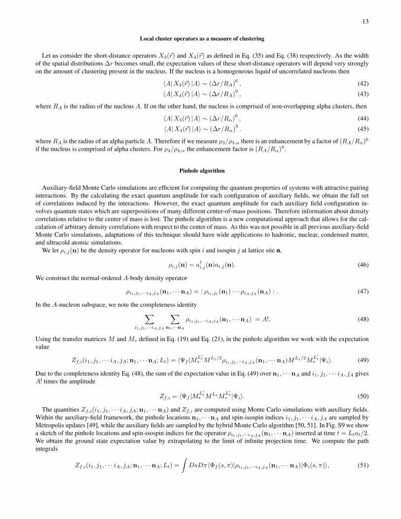
As discussed in the main text, from the A-body density information we can view the triangular shapes formed by the threespin-up protons in the carbon isotopes. The positions of the three spin-up protons serve as a measure of the alpha clustergeometry. In Fig. S10 we sketch a typical configuration of the protons (red) and neutrons (blue) with the arrows indicating upand down spins in 12C. The three spin-up protons form the vertices of a triangle, and this is indicated by the orange triangle inFig. S10. When collecting the lattice simulation data, we rotate the triangle so that the longest side lies on the x-axis. We alsorescale the triangle so the longest side has length one, and flip the triangle, if needed, so that the third spin-up proton is in theupper half of the xy-plane.

FIG. S10. We sketch a typical configuration of the protons (red) and neutrons (blue) in 12C, with the arrows indicating up and down spins. Thetriangle of spin-up protons is indicated by the orange triangle.

Form factors and radii

From the density distribution of the protons relative to the center of mass, we compute the Fourier transform to determine theelectric form factor, F (q), where q is the momentum transfer. In order to reduce systematic errors due to the lattice spacing, weperform a least squares fit of the density distribution using a two-parameter Fermi model,

ρ(r) =ρ0

1 + e(r−c)/z, (57)

and then Fourier transform to momentum space. The results are shown in Fig. S11.From the density distribution of protons and neutrons, we also compute the root-mean-square (rms) radius for the proton

and neutron distributions at leading order. The results are shown in Table I. The shown error bars include Monte Carlo errorsas well as errors due to extrapolation to infinite projection time. For comparison we show the rms charge radius observed inelectron scattering experiments. We find reasonable agreement between the 12C and 14C proton radii at leading order and thecorresponding observed charge radii.

[1] K. I. H. Horiuchi and K. Kato, Prog. Theor. Phys. Supplement 192, 1 238 (2012).

16

FIG. S11. The magnitude of the 12C electric form factor, |F (q)|, versus momentum transfer q in units of fm−1. The error bars indicate onestandard deviation errors from the stochastic noise of the Monte Carlo simulations. For comparison we also show experimental results [55].

0 0.5 1 1.5 2 2.5 3

q (fm-1)

10-4

10-3

10-2

10-1

100

|F(q

)|experimentL

t = 7

Lt = 9

Lt = 11

Lt = 13

Lt = 15

FIG. S12. The magnitude of the 14C electric form factor, |F (q)|, versus momentum transfer q in units of fm−1. The error bars indicate onestandard deviation errors from the stochastic noise of the Monte Carlo simulations. For comparison we also show experimental results [32].

0 0.5 1 1.5 2 2.5 3

q (fm-1)

10-4

10-3

10-2

10-1

100

|F(q

)|

experimentL

t = 7

Lt = 9

Lt = 11

Lt = 13

Lt = 15

TABLE I. Observed charge radii from electron scattering and proton and neutron radii at leading order.

nucleus observed charge radius proton radius (LO) neutron radius (LO)12C 2.472(16) fm [56], 2.481(6) fm [57] 2.40(7) fm 2.39(5) fm14C 2.497(17) fm [56] 2.43(7) fm 2.56(7) fm16C — 2.46(10) fm 2.65(8) fm

[2] C. Beck, ed., Clusters in Nuclei, vol. 3 of Lecture Notes in Physics (Springer-Verlag, 2014).[3] Y. Funaki, H. Horiuchi, and A. Tohsaki, Prog. Part. Nucl. Phys. 82, 78 (2015).[4] M. Freer, H. Horiuchi, Y. Kanada-En’yo, D. Lee, and U.-G. Meißner (2017), 1705.06192.[5] F. Hoyle, Astrophys. J. Suppl. 1, 121 (1954).[6] C. Cook, W. A. Fowler, C. C. Lauritsen, and T. Lauritsen, Phys. Rev. 107, 508 (1957).

17

[7] C. Romero-Redondo, S. Quaglioni, P. Navratil, and G. Hupin, Phys. Rev. Lett. 113, 032503 (2014), 1404.1960.[8] P. Maris, J. P. Vary, A. Calci, J. Langhammer, S. Binder, and R. Roth, Phys. Rev. C90, 014314 (2014), 1405.1331.[9] T. Dytrych, P. Maris, K. D. Launey, J. P. Draayer, J. P. Vary, D. Langr, E. Saule, M. A. Caprio, U. Catalyurek, and M. Sosonkina, Comput.

Phys. Commun. 207, 202 (2016), 1602.02965.[10] T. Duguet, V. Soma, S. Lecluse, C. Barbieri, and P. Navratil (2016), 1611.08570.[11] S. R. Stroberg, A. Calci, H. Hergert, J. D. Holt, S. K. Bogner, R. Roth, and A. Schwenk, Phys. Rev. Lett. 118, 032502 (2017), 1607.03229.[12] R. F. Garcia Ruiz et al., Nature Phys. 12, 594 (2016), 1602.07906.[13] G. Hagen, G. R. Jansen, and T. Papenbrock, Phys. Rev. Lett. 117, 172501 (2016), 1605.01477.[14] S. Elhatisari et al., Phys. Rev. Lett. 117, 132501 (2016), 1602.04539.[15] K. D. Launey, T. Dytrych, and J. P. Draayer, Prog. Part. Nucl. Phys. 89, 101 (2016), 1612.04298.[16] Y. Yoshida and Y. Kanada-En’yo (2016), 1609.01407.[17] H. Feldmeier and T. Neff (2016), 1612.02602.[18] P. Schuck, Y. Funaki, H. Horiuchi, G. Roepke, A. Tohsaki, and T. Yamada, Phys. Scripta 91, 123001 (2016), 1702.02191.[19] T. Yoshida, N. Shimizu, T. Abe, and T. Otsuka, J. Phys. Conf. Ser. 569, 012063 (2014).[20] A. Lovato, S. Gandolfi, J. Carlson, S. C. Pieper, and R. Schiavilla, Phys. Rev. Lett. 117, 082501 (2016), 1605.00248.[21] E. Epelbaum, H. Krebs, D. Lee, and U.-G. Meißner, Phys. Rev. Lett. 106, 192501 (2011), 1101.2547.[22] E. Epelbaum, H. Krebs, T. Lahde, D. Lee, and U.-G. Meißner, Phys. Rev. Lett. 109, 252501 (2012), 1208.1328.[23] E. Epelbaum, H. Krebs, T. A. Lahde, D. Lee, and U.-G. Meißner, Phys. Rev. Lett. 110, 112502 (2013), 1212.4181.[24] E. Epelbaum, H. Krebs, T. A. Lahde, D. Lee, U.-G. Meißner, and G. Rupak, Phys. Rev. Lett. 112, 102501 (2014), 1312.7703.[25] E. Wigner, Phys. Rev. 51, 106 (1937).[26] S. Elhatisari, D. Lee, G. Rupak, E. Epelbaum, H. Krebs, T. A. Lahde, T. Luu, and U.-G. Meißner, Nature 528, 111 (2015), 1506.03513.[27] A. Rokash, E. Epelbaum, H. Krebs, and D. Lee (2016), 1612.08004.[28] C. L. Zhang, B. Schuetrumpf, and W. Nazarewicz, Phys. Rev. C94, 064323 (2016), 1607.00422.[29] R. B. Wiringa, S. C. Pieper, J. Carlson, and V. R. Pandharipande, Phys. Rev. C62, 014001 (2000), nucl-th/0002022.[30] M. A. Belushkin, H.-W. Hammer, and U.-G. Meißner, Phys. Rev. C75, 035202 (2007), hep-ph/0608337.[31] R. Pohl et al., Nature 466, 213 (2010).[32] F. J. Kline, H. Crannell, J. T. O’ Brien, J. McCarthy, and R. R. Whitney, Nucl. Phys. A209, 381 (1973).[33] L. R. Hafstad and E. Teller, Phys. Rev. 54, 681 (1938).[34] H. G. Bohlen, T. Dorsch, T. Kokalova, W. von Oertzen, C. Schulz, and C. Wheldon, Nucl. Phys. A787, 451 (2007).[35] H. G. Bohlen et al., Nucl. Phys. A722, C3 (2003).[36] M. Freer, AIP Conf. Proc. 1072, 58 (2008).[37] D. J. Marin-Lambarri, R. Bijker, M. Freer, M. Gai, T. Kokalova, D. J. Parker, and C. Wheldon, Phys. Rev. Lett. 113, 012502 (2014),

1405.7445.[38] E. Epelbaum, H. Krebs, D. Lee, and U.-G. Meißner, Eur. Phys. J. A45, 335 (2010), 1003.5697.[39] V. G. J. Stoks, R. A. M. Kompl, M. C. M. Rentmeester, and J. J. de Swart, Phys. Rev. C48, 792 (1993).[40] S. Konig, H. W. Grießhammer, H. W. Hammer, and U. van Kolck, Phys. Rev. Lett. 118, 202501 (2017), 1607.04623.[41] J.-W. Chen, D. Lee, and T. Schafer, Phys. Rev. Lett. 93, 242302 (2004), nucl-th/0408043.[42] D. Lee, Phys. Rev. Lett. 98, 182501 (2007), nucl-th/0701041.[43] D. Lee, Prog. Part. Nucl. Phys. 63, 117 (2009), 0804.3501.[44] J. Hubbard, Phys. Rev. Lett. 3, 77 (1959).[45] R. L. Stratonovich, Soviet Phys. Doklady 2, 416 (1958).[46] S. E. Koonin, Journal of Statistical Physics 43, 985 (1986), ISSN 0022-4715.[47] K. G. Wilson, Phys. Rev. 179, 1499 (1969).[48] W. Zimmermann, Annals of Physics 77, 570 (1973), ISSN 0003-4916.[49] W. K. Hastings, Biometrika 57, 97 (1970).[50] S. Duane, A. D. Kennedy, B. J. Pendleton, and D. Roweth, Phys. Lett. B195, 216 (1987).[51] S. Gottlieb, W. Liu, D. Toussaint, R. L. Renken, and R. L. Sugar, Phys. Rev. D35, 2531 (1987).[52] D. Lee, Lect. Notes Phys. 936, 237 (2017), 1609.00421.[53] N. Metropolis, A. W. Rosenbluth, M. N. Rosenbluth, A. H. Teller, and E. Teller, J. Chem. Phys. 21, 1087 (1953).[54] S. Konig and D. Lee (2017), 1701.00279.[55] I. Sick and J. S. Mccarthy, Nucl. Phys. A150, 631 (1970).[56] L. A. Schaller, L. Schellenberg, T. Q. Phan, G. Piller, A. Ruetschi, and H. Schneuwly, Nucl. Phys. A379, 523 (1982).[57] I. Sick, Phys. Lett. 116B, 212 (1982).