AAS 15-329

CONTROL METRIC MANEUVER DETECTION WITH GAUSSIANMIXTURES AND REAL DATA

Andris D. Jaunzemis∗, Midhun Mathew†, Marcus J. Holzinger‡

The minimum-fuel distance metric provides a natural tool with which to as-sociate space object observation data. A trajectory optimization and anomaly hy-pothesis testing algorithm is developed based on the minimum-fuel distance metricto address observation correlation under the assumption of optimally maneuver-ing spacecraft. The algorithm is tested using inclination-change scenarios withboth synthetic and real data gathered from the Wide Area Augmentation System(WAAS). Comparisons to other commonly-used association metrics such as Ma-halanobis distance reveal less sensitivity in anomaly detection but improved con-sistency with respect to observation cadence, while providing added data throughthe reconstruction of the optimal maneuver. Non-Gaussian boundary conditionsare also approached through an analytical approximation method, yielding signif-icant computational complexity improvements.

INTRODUCTION & BACKGROUND

Correlating on-orbit observations and detecting space object maneuvers is a challenging endeavorin the Space Situational Awareness (SSA) field. There are currently at least 17,000 trackable on-orbit objects, 1,000 of which are active,1, 2 and these numbers are expected to grow significantly dueto improved tracking capabilities, new launches, and continued debris generation.3 Predicting con-junction events is a difficult task;4 however, recent events highlight the mutual interest that nationaland private operators share for accurate object correlation and maneuver detection capability.5

This study examines a novel method for correlating space object tracks with known residentspace objects (RSOs) and characterizing and reconstructing RSO maneuvers. The problem of as-sociating uncorrelated tracks (UCTs) over large time periods is particularly difficult when objectsmaneuver during observation gaps. Even relatively small station-keeping maneuvers at geostation-ary Earth orbit (GEO) can result in position discrepancies of many kilometers after an observationgap. UCT correlation is further confounded by state estimate uncertainties.6 Since both the ini-tial and final UCTs are best estimates, with associated uncertainty distributions, the question ofcorrelation becomes difficult to answer in operational settings, particularly in densely-populated re-gions of the space environment. Given a propagated best estimate of the state and its associateddistribution, correlating UCTs tests whether a new observation (with its associated uncertainty) isa previously observed object, and if not, determines the discrepancy. There are many distance- or

∗Graduate Research Assistant, Georgia Institute of Technology, Atlanta, GA, AIAA Student Member†Graduate Research Assistant, Georgia Institute of Technology, Atlanta, GA, AIAA Student Member‡Assistant Professor, Georgia Institute of Technology, Atlanta, GA, AIAA Senior Member

1

pseudo-distance metrics that may be used to measure the discrepancy between two state distribu-tions (e.g. Mahalanobis distance). Problematically, none of these distance metrics directly quantifythe level of propulsive effort required to cause the observed state change.

In this study, the minimum-fuel control distance metric is utilized in a hypothesis testing algo-rithm to approach data association and maneuver detection problems. Since on-board fuel remains ascarce commodity for operational spacecraft, operators are likely to execute optimal or near-optimalmaneuvers.6 Under the assumptions of optimal control, multiple deterministic observations can berelated by computing the control effort required for a spacecraft trajectory to meet those boundaryconditions. This approach necessitates the reconstruction of a minimum-fuel trajectory consistentwith the a-priori information and new observations. Holzinger has shown, through the properties ofstrict positivity, symmetry, and triangle inequality, that control performance is a metric,6 allowingcomparisons to other commonly used distance metrics. The inputs to the maneuver detection al-gorithm are two UCTs, containing the estimated states and associated covariances of the trajectoryboundary conditions. An optimal connecting trajectory is then computed in a minimum-quadratic-control trajectory optimization implementation. The resulting optimal trajectory is used to generatea control cost distribution associated with perturbations in the boundary conditions based on theinput covariances.6 The optimal control cost and control cost distribution are used to test the hy-pothesis that a maneuver occurred and complete the maneuver detection task.6, 7, 8 This frameworkis tested using simulated and real-world operational data.

In addition to the minimum-fuel control distance maneuver detection algorithm, this study en-deavors to analytically incorporate non-Gaussian boundary conditions for increased realism in rep-resenting the boundary condition UCTs. State uncertainty is a fundamental problem of space situa-tional awareness in the cases of track association and maneuver detection.9 The probability densityfunction must be accurately represented to address the requirement of uncertainty consistency. Ini-tially, the state uncertainty may be assumed to be Gaussian, which is often appropriate for residentspace objects. However, the dynamics governing the orbital mechanics (e.g. gravity, drag, thirdbody perturbations, etc.) are nonlinear. After propagation for some time, the state uncertainty maybecome non-Gaussian.9 Gaussian mixtures provide a convenient method to represent non-Gaussianuncertainties and to generate a combined probability model for the total overlapping uncertaintiesof each state. The uncertainty in measurements may be non-Gaussian, especially after propaga-tion of the previous best estimate, or there may be multiple sensor measurements. However, manyprobability density functions can be closely approximated by a Gaussian mixture.9 Multiple stateestimate and covariance pairs can be used to construct a Gaussian mixture which can more accu-rately describe the UCT and measurement uncertainties.

The contributions of this paper are 1) the implementation of a maneuver detection hypothesistesting algorithm using the minimum-fuel control distance metric and its evaluation using bothsynthetic and real-world data, 2) the comparison of the minimum-fuel control distance metric toother data association approaches (e.g. Euclidean and Mahalanobis distance), and 3) the statisticaltreatment of control distributions using Gaussian mixtures for non-Gaussian boundary conditions.

THEORY

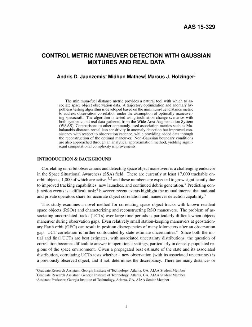
The algorithm described in this section endeavors to determine a correlation between two UCTsunder the hypothesis that the tracks belong to the same maneuverable space object and the object hasmaneuvered optimally between the observations. As pictured in Figure 1, an uncorrelated track hasbeen generated at time tA with best-estimate state xA and covariance PA. This track has been prop-

2

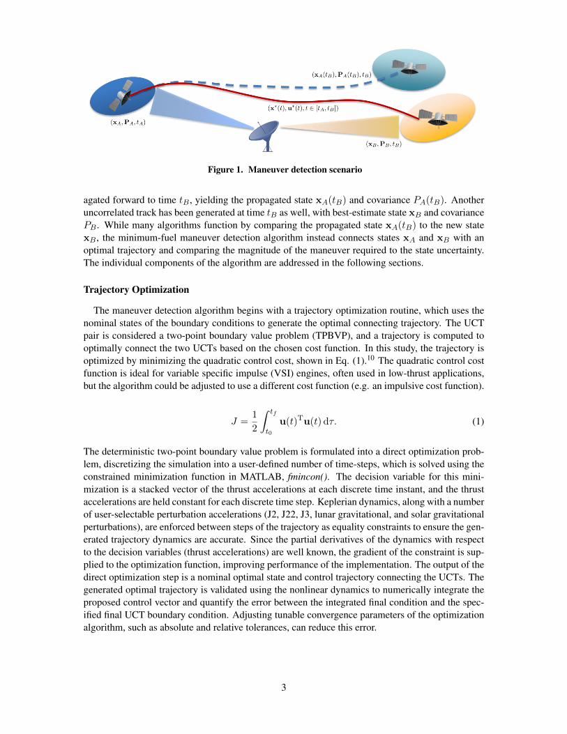
Figure 1. Maneuver detection scenario

agated forward to time tB , yielding the propagated state xA(tB) and covariance PA(tB). Anotheruncorrelated track has been generated at time tB as well, with best-estimate state xB and covariancePB . While many algorithms function by comparing the propagated state xA(tB) to the new statexB , the minimum-fuel maneuver detection algorithm instead connects states xA and xB with anoptimal trajectory and comparing the magnitude of the maneuver required to the state uncertainty.The individual components of the algorithm are addressed in the following sections.

Trajectory Optimization

The maneuver detection algorithm begins with a trajectory optimization routine, which uses thenominal states of the boundary conditions to generate the optimal connecting trajectory. The UCTpair is considered a two-point boundary value problem (TPBVP), and a trajectory is computed tooptimally connect the two UCTs based on the chosen cost function. In this study, the trajectory isoptimized by minimizing the quadratic control cost, shown in Eq. (1).10 The quadratic control costfunction is ideal for variable specific impulse (VSI) engines, often used in low-thrust applications,but the algorithm could be adjusted to use a different cost function (e.g. an impulsive cost function).

J =1

2

∫ tf

t0

u(t)Tu(t) dτ. (1)

The deterministic two-point boundary value problem is formulated into a direct optimization prob-lem, discretizing the simulation into a user-defined number of time-steps, which is solved using theconstrained minimization function in MATLAB, fmincon(). The decision variable for this mini-mization is a stacked vector of the thrust accelerations at each discrete time instant, and the thrustaccelerations are held constant for each discrete time step. Keplerian dynamics, along with a numberof user-selectable perturbation accelerations (J2, J22, J3, lunar gravitational, and solar gravitationalperturbations), are enforced between steps of the trajectory as equality constraints to ensure the gen-erated trajectory dynamics are accurate. Since the partial derivatives of the dynamics with respectto the decision variables (thrust accelerations) are well known, the gradient of the constraint is sup-plied to the optimization function, improving performance of the implementation. The output of thedirect optimization step is a nominal optimal state and control trajectory connecting the UCTs. Thegenerated optimal trajectory is validated using the nonlinear dynamics to numerically integrate theproposed control vector and quantify the error between the integrated final condition and the spec-ified final UCT boundary condition. Adjusting tunable convergence parameters of the optimizationalgorithm, such as absolute and relative tolerances, can reduce this error.

3

The optimal states x∗(t) and controls u∗(t) for tA ≤ t ≤ tB are then used to compute a time-history of optimal control costates p∗(t). The costates are constructed by guessing a costate tra-jectory based on the optimal control trajectory and then modifying the costates through an iterativeleast-squares method until the control cost is within a user-defined convergence tolerance of theoptimal trajectory. As an additional check, the new optimal costate trajectory is compared to theoriginal optimal trajectory to ensure the endpoint error has not changed significantly.

Control Cost Distribution Generation

Using the optimal state and costate trajectory (x∗(t) and p∗(t)), uncertainties in position andvelocity are included to generate an approximate probability distribution of the control cost. This isaccomplished by linearizing about the nominal optimal trajectory and applying perturbations in theinitial and final conditions based on the covariance of each associated UCT. Performing this manytimes generates a distribution of optimal or sub-optimal trajectories, and the control cost associatedwith these perturbed trajectories can be computed using the results from Holzinger et al.6 Keyresults used in generating and analyzing the control cost distributions for this work are reiteratedhere. In general, the cost distribution can be written succinctly as shown in Eq. (2):

J = J∗ + δJ (2)

where δJ is a perturbation to the optimal cost, J∗, caused by variations in the initial and finalboundary conditions. This cost function is utilized by taking the Taylor series expansion up to thefirst-order terms to approximate a value for the perturbed cost. From Holzinger et al.,6 there existsa function Λ(t, t0), shown in Eq. (3), that maps variations in initial and final states to variations inthe costate δp(t) at time t.

Λ(t, t0) = Φpx(t, t0)−Φpp(t, t0)Φxp(tf , t0)†Φxx(tf , t0)Φpp(t, t0)Φxp(tf , t0)

† (3)

Note that this function is composed of portions of the state transition matrix. The pseudoinverseterm Φxp(tf , t0)

† is not guaranteed to exist for arbitrary systems, but for present purposes it isassumed to exist.6 The cost function in Eq. (1) is expanded by substituting u(τ) = u∗(τ) + δu(τ):

J ≈ 1

2

∫ tf

t0

u∗(τ)Tu∗(τ)dτ +

∫ tf

t0

u∗(τ)T∂f

∂u

T

Λ(τ, 0)δzdτ (4)

+1

2

∫ tf

t0

δzTΛ(τ, 0)T∂f

∂u

∂f

∂u

T

Λ(τ, 0)δzdτ

where δzT =[δxT

0 δxTf

]∈ R2n. Since δz is independent of τ , the cost function can be rewritten

using the following definitions:

J∗ =1

2

∫ tf

t0

u∗(τ)Tu∗(τ)dτ (5)

ω(tf , t0) =

∫ tf

t0

Λ(τ, 0)T∂f

∂uu∗(τ)dτ (6)

Ω(tf , t0) =1

2

∫ tf

t0

Λ(τ, 0)T∂f

∂u

∂f

∂u

T

Λ(τ, 0)dτ (7)

4

Note that J∗ is the optimal cost of the optimal trajectory (x∗(t),p∗(t)) without boundary-conditionvariations. The cost function in Eq. (4) is rewritten in a more compact form:

J ≈ J∗ + ω(tf , t0)Tδz + δzTΩ(tf , t0)δz (8)

The process for computing the control cost distribution is simplified using statistical treatmentsfor the mean (µJ ) and variance (σ2J ) to sample and generate a cost distribution. The process forcalculating the mean and standard deviation from the optimal trajectory and covariance is based onEqns. (9) and (10) respectively.6

µJ = J∗ + Tr [ΩPz] (9)

σ2J = ωTPzω + 2Tr [ΩPzΩPz] (10)

If it is assumed that the boundary conditions are independent of each other and do not share infor-mation, Pz ∈ R12×12 is composed of PA in the top-left 6 × 6 block and PB in the bottom-right6 × 6 block. Using the analytical values for the first and second moments of the distribution, aGaussian approximation of the cost distribution is generated. The distribution of control costs asso-ciated with state uncertainty, found by subtracting the optimal control cost J∗ from cost distributionJ , is termed the uncertainty cost distribution. Therefore, from Eq. (2), the normally distributedperturbation in the cost function is δJ ∼ N (Tr [ΩPz] , σ2J). In this study, the expectation of thiscontrol cost perturbation is referred to as the minimum detectable control cost, defined in Eq. (11):

Jdet = Tr [ΩPz] (11)

so-called because it is a threshold used in the anomaly detection algorithm to determine if the stateuncertainty accounts for the state change.

In order to validate the uncertainty cost distribution, a more exact distribution was constructedby sampling locally around the optimal trajectory with a random stacked vector of initial and finalstate perturbations, δz ∼ N (0,Pz). The quadratic cost due to this state uncertainty can then beapproximated as shown in Eq. (12):6

δJ ≈ ωTδz + δzTΩδz (12)

In this implementation, the analytical mean and standard deviation are used to size the range forthe histogram used in generating the normalized PDF. Furthermore, the minimum detectable costfor this distribution can then found using the cumulative distribution function (CDF). The minimumdetectable control cost (Jdet) is defined, similar to the Gaussian approximation, as the expectationof the uncertainty control cost distribution. In testing, the Gaussian approximation agreed well withthe locally sampled distribution, producing nearly identical cost distributions, thereby validating theuse of the Gaussian approximation in this study.

Anomaly Detection

Using the optimal control cost and uncertainty control cost distribution generated in the previoussteps, the algorithm can now perform the anomaly hypothesis testing. In this algorithm, hypothesistesting involves the computation of the cumulative distribution function, as shown in Eq. (13):8

pA =

∫ J∗

−∞f (J) dJ (13)

5

The hypothesis being tested is that the state difference observed between two UCTs is attributableto an anomaly (e.g. controlled maneuver, unmodeled perturbations, etc.) as opposed to quiescentpropagation and measurement uncertainty. This hypothesis is tested by comparing the magnitude ofthe optimal control cost to the uncertainty control cost distribution to determine whether the controlrequired to connect the UCTs is buried in the noise of the uncertainty. This comparison can beeasily seen in the CDF generated from the uncertainty cost distribution, and the probability that thehypothesis is true, termed the probability of anomaly, is computed by finding the value of the CDFat a control cost value equal to the optimal control cost, as in Eq. (13). A trajectory with a nominalcontrol cost (J∗) greater than the minimum detectable cost (Jdet) has a higher probability of beingthe result of an anomaly and not the result of propagated boundary condition uncertainty.

A sample result to illustrate this method is shown in Figure 2. The figure shows the PDF and CDFfor the quadratic control cost as a function of control cost. The minimum detectable control costcan be seen as the control cost where the CDF equals 0.5. The vertical dashed line represents thenominal optimal control cost for that maneuver. On the CDF plot, it can be seen that the intersectionof the CDF and nominal quadratic cost yields a probability of anomaly of approximately 0.75, or75%. The uncertainty control cost CDF is the key to computing the probability that a maneuver hasoccurred for a given optimal trajectory and state uncertainty.

Figure 2. Notional control cost distribution (normalized PDF and CDF)

Since the control cost and cost distribution magnitudes vary widely with both simulation timehorizon and UCT uncertainty, it is useful to define an anomaly detectability ratio (ADR) as the ratioof the nominal optimal control cost to the minimum detectable cost, as shown in Eq. (14):

ADR =J∗

Jdet=

J∗

Tr [ΩPz](14)

If the nominal optimal control cost is equal to the minimum detectable quadratic cost for a givenstate uncertainty, then the detectability ratio is 1 and the probability of anomaly is equal to 0.5,or 50%, as seen in Figure 2. That is to say, there is an equal probability that the observed statechange is caused by an anomaly (such as a maneuver) or explained by uncertainty in the initial andfinal states. As the nominal control cost increases with respect to the minimum detectable cost,the detectability ratio increases and the probability that the state change is caused by an anomalyincreases. Eventually, the nominal cost becomes substantially larger than the cost due to uncertainty,so the probability that state uncertainty could cause the state change is approximately zero and theprobability of anomaly approaches 1.0, or 100%.

6

Maneuver Detection Algorithm Framework

The entire maneuver detection algorithm is assembled as shown in Figure 3. The inputs to thealgorithm are a pair of UCTs, containing the state, covariance, and time data for each track. Thetrajectory optimization is first performed on the best-estimate states to extract an optimal directtrajectory, which is then refit to calculate the adjoints. Then the cost distribution is generated to testthe anomaly hypothesis and determine the probability that an anomaly has occurred. The output ofthe algorithm is the probability that the anomaly hypothesis was true, PA. Stated differently, this isthe probability that a maneuver has occurred between the UCTs.

Figure 3. Minimum-fuel metric maneuver detection algorithm

Given an optimal trajectory and uncertainty in the boundary conditions, this method can computethe probability that an observed state change is due to quiescent propagation or active maneuvering,thus addressing the maneuver detection goal. Additionally, if it is determined that boundary con-dition uncertainty cannot account for the state change, and a maneuver or unmodeled perturbationmust have occurred, the minimum magnitude and time history of the potential maneuver can be de-termined from the computed optimal trajectory, characterizing any such maneuver. Furthermore, ifthe user has knowledge of the maneuvering capabilities of the RSO and the maneuver is determinedto be impossible for that specific RSO, this method can be used to associate (or disassociate) UCTsbased on the control authority required.

Quadratic Control Distance Distributions using Gaussian Mixtures

By employing Gaussian mixtures to model uncertainties, the accuracy of the initial and final con-ditions can be improved. For boundary conditions described by Gaussian distributions, the TPBVPuses the trajectory connecting the best-estimate, or mean, state and incorporates the correspondingcovariance. However, a single Gaussian distribution might not accurately describe the state or prop-erly incorporate the uncertainties. To properly address non-Gaussian uncertainty, potential TPBVPsbetween separate regions of uncertainties must be considered. Using Gaussian mixtures creates acombined probability model for the non-Gaussian distributions.

Gaussian mixture models are defined as the weighted sum of a set of multivariate normal densityfunctions. In this application, each normal distribution represents a component of the boundarycondition defined by the Gaussian mixture. In general, a multivariate Gaussian mixture may berepresented by the density function in Eq. (15).

f(x) =

n∑i=1

wifi(x) (15)

7

where fi(x) = N (µi, σ2i ) is a Gaussian density function with mean µi and variance σ2i , and

w1, . . . , wn is a set of weightings such that wi ≥ 0 and∑n

i wi = 1. A random variable (ζ)sampled from this mixture may be defined as seen in Eq. (16).

ζ ∼n∑

i=1

wiN (µi, σ2i ) (16)

In order to improve accuracy in the modeling of initial and final condition state uncertainties, thenormal distribution assumption can be relaxed using Gaussian mixtures as described below. Whenconsidering boundary conditions defined by Gaussian mixtures, a combined quadratic control costfor the entire mixture must be defined. Instead of calculating the quadratic cost as a function ofthe cost from each trajectory connecting an initial component Gaussian distribution to each finalGaussian distribution, a trajectory connecting the mean states of the initial and final boundary con-ditions is used. The mean state of a boundary condition is computed as the weighted average of thebest-estimate states of each component Gaussian distribution. The mean states enable the trajec-tory to be reduced to a single two-point boundary value problem, constructing the cost distributionby linearizing about this mean connecting trajectory and sampling initial and final states from thenon-Gaussian boundary conditions.

Figure 4. Gaussian Mixture scenario geometry

The method for constructing this cost distribution is based off a similar derivation for Gaussianinitial and final distributions,6 and is described below. Figure 4 shows a notional depiction of thekey variables introduced in the Gaussian mixture approximation. The expected value of the statesat each boundary condition Gaussian mixture is computed, and the optimal trajectory between thesepoints is computed to find the nominal optimal trajectory (x∗(t),u∗(t)). Additionally, the deviationof the mean of each individual Gaussian from the expected value of each boundary condition stateis computed as µi and µj for the initial and final conditions, respectively.

The quadratic control cost function, in Eq. (17), can be expanded by decomposing the controleffort u(t) into three components as shown in Eq. (18).

J =1

2

∫u(τ)Tu(τ)dτ (17)

u(t) = u∗(t) + uij + δu(t) (18)

= − ∂f

∂u

T (p∗(t) + pij(t) + δp(t)

)(19)

8

In Eq. (18), the term uij(t) represents the control cost attributable to the µi and µj , the variationsin mean state of Gaussian initial component i and final component j from the expected value of theGaussian mixture boundary conditions. Likewise, δu(t) is the control cost attributable to δx0 andδxf , the variations in sampled state from boundary condition uncertainty. These components canbe computed as shown in Eqns. (20) and (21) using Λ(t, t0) from Eq. (3).

uij(t) = − ∂f

∂u

T

Λ(t, t0)

[µi

µj

](20)

δu(t) = − ∂f

∂u

T

Λ(t, t0)

[δx0

δxf

](21)

The following vectors are defined for ease of notation:

µij =

[µi

µj

](22)

δz =

[δx0

δxf

](23)

where µij is a constant vector for each i,j boundary condition pair and δz is sampled from theboundary condition uncertainties such that δx0 ∼

∑ni=1wiN (0,Pi) and δxf ∼

∑mj=1wjN (0,Pj).

Substituting the above relationships into Eq. (17), expanding, and introducing the functions ω(t, t0)and Ω(t, t0) from Eqns. (6) and (7), the quadratic control cost for a single term of the Gaussian mix-ture connecting Gaussian initial distribution i to Gaussian final distribution j is:

Jij = J∗ + ω(tf , t0)Tδz + 2µT

ijΩ(tf , t0)δz + ω(tf , t0)Tµij (24)

+ µijΩ(tf , t0)µij + δzTΩ(tf , t0)δz

The quadratic cost is dependent upon J∗, Ω, and ω of the nominal optimal trajectory connecting theexpected value initial and final states. Combining terms, the cost Jij can be re-written in a formatsimilar to the strictly Gaussian result from Holzinger et al.,6 as shown in Eq. (25).

Jij = J∗ + ω(tf , t0)T(µij + δz) + (µij + δz)TΩ(tf , t0)(µij + δz) (25)

From Holzinger et al.6 Appendix B, the analytic first and second moments of Jij are:

E [Jij ] = µJ,ij = J∗ + ωTµij + µTijΩijµij + Tr [ΩijPz,ij ] (26)

E[J2ij

]= σ2J,ij =

(ωT + 2µT

ijΩ)T

Pz,ij

(ωT + 2µT

ijΩ)

+ 2Tr [ΩPz,ijΩPz,ij ] (27)

Then, the total cost of all i initial boundary conditions and j final boundary conditions is theweighted sum of the individual costs between each i and j:

J =∑i

∑j

wiwjJij (28)

where wi is the weight of the ith initial boundary condition and wj is the weight of the jth finalboundary condition. Thus, the analytic expected value of the initial and final Gaussian sum bound-

9

ary condition may be written as:

E [J ] = E

∑i

∑j

wiwjJij

=∑i

∑j

wiwjE [Jij ]

=∑i

∑j

wiwjµJ,ij (29)

which leads to the final result:

µJ =∑i

∑j

wiwj

(J∗ + ωTµij + µT

ijΩµij + Tr [ΩPz,ij ])

(30)

RESULTS

To validate the algorithm implementation, test cases are used to identify the limits and perfor-mance of the algorithm. For each case tested, a nominal UCT boundary condition uncertainty(covariance matrix) is parameterized using a scalar multiplier to examine the effects of uncertaintyon anomaly detection. Similarly, to examine the effects of duration between UCTs, each scenariosimulates various time intervals between UCTs of up to 48 hours. The uncertainty control costdistributions at the boundary conditions are computed and compared to the deterministic optimalmaneuver control cost to test the maneuver (or anomaly) hypothesis. The results include a syn-thetic (simulated) scenario and real-world data. Since real-world operational data is available, thesynthetic scenario is constructed to closely resemble that scenario for comparison purposes.

Synthetic Scenario: Inclination Correction

The first test case studied is a simulated inclination correction. For this purpose, a geostationarysatellite inclination change scenario was constructed, similar to the real-world data available. Inthe scenario, UCTs are initialized with identical orbit elements except for the inclination and trueanomaly. The initial inclination is set to 0.02 degrees, while the final inclination is set to 0 degrees,values chosen to reflect the available real data. The change in true anomaly is related to the durationof the simulation, which is another variable in the simulation. This set of boundary conditions allowsfor the simulation of an inclination-change station-keeping maneuver for varying observation gapsto assess the detectability of this maneuver.

A sensitivity study is conducted to generate confidence curves of probability of anomaly basedon a) maneuver detectability ratio and b) UCT time separation. The boundary condition uncertaintyfor this particular scenario is assumed Gaussian and is initialized at 1 meter in position and 0.01meters-per-second in velocity, as shown in Eq. (31):

PA = PB = diag(α2, α2, α2, (0.01α)2, (0.01α)2, (0.01α)2

)(31)

where α is the scalar that is varied between scenarios to change the uncertainty (and modulate thedetectability ratio). The scalar is allowed to vary logarithmically from 1 to 103, a range determinedby trial and error to cover a wide range of detectability ratio values (from near-zero to well above9). This corresponds to maximum boundary condition position and velocity uncertainties of 10kilometers and 100 meters-per-second, respectively.

10

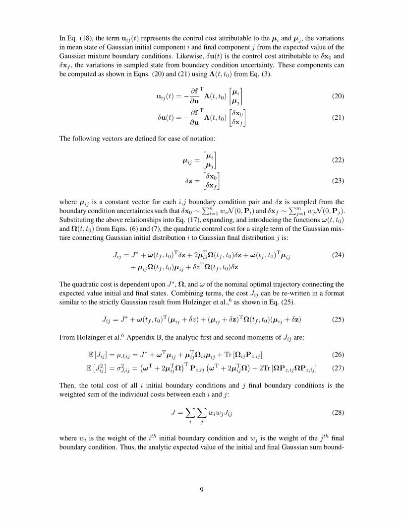
Preliminary results from this scenario were used for validation of the algorithm framework, usinga nominal scenario with the initial condition 30 minutes before the ascending node passage andthe final condition 30 minutes after the ascending node passage. The probability of anomaly forthis scenario using different detectability ratios is shown in Figure 5. As desired, the probability ofanomaly at a detectability ratio of 1 is exactly 0.5, so there is an equal likelihood that the observedstate change is caused by a control maneuver or uncertainty at this test case. As the detectabilityratio increases above 1, the probability that a maneuver occurred increases, and opposite below adetectability ratio of 1.

Figure 5. Probability of Anomaly vs Detectability Ratio, Synthetic Scenario (1 hoursimulation duration)

To test the result validity, an upper-bound cost can be applied based on the quadratic cost from themaneuver optimization.11 Additionally, the continuously-thrusting maneuver cost should be lower-bounded by the impulsive maneuver cost for an inclination change of 0.02 degrees. These sanitychecks are shown in Table 1, and the trajectory (actual) cost is within the acceptable range.

Table 1. Simulated Maneuver Control Cost and Comparisons

Parameter Value Units

Quadratic Control Cost 1.609022285× 10−4 m2

s3

Impulsive ∆V 1.0732610 ms

Actual ∆V 1.0763310 ms

Upper-bound ∆V 1.0763345 ms

Having analyzed the performance of the algorithm using a nominal scenario, the next step is toexamine the sensitivity of the algorithm to the time between UCT observations. To perform thissensitivity study, the initial and final conditions are varied to change simulation duration, keepingthe ascending node passage at the midpoint of the simulation duration. The initial and final timesare varied from 5 minutes before and after the ascending node (10 minute simulation duration) to24 hours before and after the ascending node (48 hour simulation duration), and the initial and finalstates are adjusted accordingly. The trajectory optimizer is not confined to a specific time withinthe simulation time window to perform the correction maneuver, and results show that the optimaltrajectories selected use the maximum thrust acceleration at the node passages. This is consistentwith intuition since an impulsive inclination-change maneuver would be performed entirely at the

11

Figure 6. Anomaly detection probability vs Anomaly Detectability Ratio and Uncer-tainty Scaling Parameter, Synthetic Scenario

node passages, so an optimal low-thrust maneuver should maximize its thrusting at the nodes.

The results of this sensitivity study are distilled in the contour plot in Figure 6. On the left-handside plot, detectability ratio and duration are varied on the x- and y-axes respectively, and the con-tours show lines of constant probability of anomaly, increasing from 0.25% to 0.99% from left toright. The contours shown represent different confidence levels (or probabilities of anomaly) thatthe state change is attributable to an anomaly such as a maneuver given the observation durationand uncertainties. The 0.5, or 50%, confidence level is a straight line at a detectability ratio of 1,as prescribed by the anomaly detection method. Otherwise, even moderate confidence levels arerelatively consistent, though a periodic behavior can be seen. The improvement in maneuver detec-tion at 12 and 36 hours coincides with the highest out-of-plane state difference between the finalobservation and propagated state estimate. Conversely, at durations of an orbit period, maneuverdetection requires lower state uncertainty because the boundary condition states are more similar.

The same sensitivity study data was plotted using α, the uncertainty scaling parameter, as thex-axis variable, shown in the right-hand side of Figure 6. Viewed as a function of uncertaintyscaling parameter, the control distance metric better shows its consistency with respect to duration,especially in comparison to the Mahalanobis distance results presented later. The difference in thetwo contours of Figure 6 reveals an issue in viewing the results as a function of ADR, since ADRis a function of both minimum detectable control distance and optimal control distance. The plotusing uncertainty scaling parameter avoids conflating these variables and emphasizes the duration-independence of the control distance metric.

This sensitivity study emphasizes an advantage of the control metric approach, which is that itperforms relatively consistently with respect to observation duration. Some previous knowledgeof the orbit is still useful in determining the validity of the maneuver detection probability results.For instance, when attempting to detect inclination change maneuvers, observations spaced at orbitperiods are not ideal because this could yield a small state difference and require lower observationuncertainty to detect maneuvers with high likelihood. Another, more obvious, result is that largermaneuvers, which yield a higher detectability ratio for the same boundary condition uncertainty,are easier to detect. This is particularly relevant for maneuvers by spacecraft with variable specific-impulse engines, where the state changes are small and spread out over a long time. Conversely,a large state-change by a nearly-impulsive maneuver could still be detected even in a short timebetween observations, if the control required for the maneuver significantly exceeds the state change

12

in the homogeneous orbit based on boundary condition uncertainty.

Real-World Data: Inclination Correction

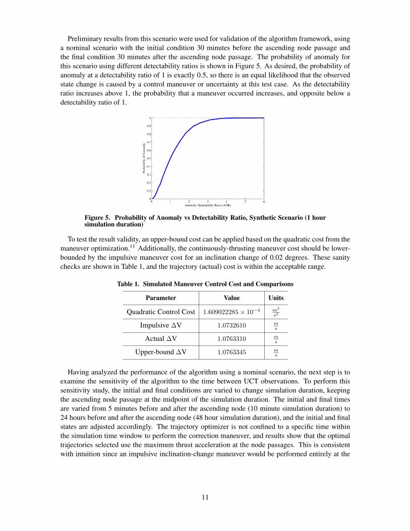
To complement the simulated scenario, the algorithm is tested using real operational data, theavailability of which drove the construction of the simulated scenario. The real data, taken fromobservations of the Galaxy 15 geostationary satellite by the Wide Area Augmentation System(WAAS), spans a month of operation and includes Earth-centered Earth-fixed (ECEF) position andvelocity, as well as radial, in-track, and cross-track (RIC) acceleration (as seen by a rotating Hillframe attached to the spacecraft). WAAS is an extremely accurate navigation system that uses anetwork of ground-based reference stations to measure small variations in GPS satellite signals todevelop Deveiation Corrections (DCs). The DCs are then broadcast by GPS satellites to improveposition accuracy calculations for WAAS-enabled GPS receivers.12

Figure 7. Cross-track Acceleration for Geosynchronous satellite, Real Data

Figure 7 shows the cross-track acceleration data for the real dataset. Inspection of the accelera-tion data reveals two large anomalous cross-track acceleration events, candidates for a North-South(inclination) station-keeping maneuver, during days 7 and 22. The selected maneuver (the peakaround day 7) resulted in a 0.03 degree inclination change, and simulation initial and final condi-tions were chosen to surround this maneuver in equal time increments around the maneuver. Thereal-world data is analyzed in a similar manner to the synthetic data: by varying boundary conditionuncertainty and time, a sensitivity study is conducted to construct probability of anomaly confidencecurves with respect to detectability ratio and simulation duration. An initial boundary condition isselected from the data given a desired time before the candidate maneuver, Therefore, the studybegins with a simulation duration of 1 hour and increases to a duration of 48 hours, spaced evenlyaround the candidate maneuver.

The results of this sensitivity study are shown in Figure 8, plotted against anomaly detectabil-ity ratio on the left and uncertainty scaling parameter on the right. The confidence-level contoursagree closely with with Figure 6 from the synthetic scenario. In testing, when many of the per-turbing accelerations were deselected, the algorithm responded by predicting higher probabilities ofanomaly at lower uncertainties, since the real spacecraft deviated from the unperturbed propagationquickly. Therefore, it is important to model the relevant dynamics perturbations for a given testcase. In this case, agreement between the simulated and operational data cases lends confidencethat the applicable perturbations have been modeled in the trajectory optimizer, and reinforces theapplicability of this algorithm to real data in operational use. Additionally, since propagated orbitalmechanics uncertainties often become non-Gaussian quickly, the Gaussian mixture approximationmethods presented in this paper provide further computationally feasible applicability to real data.

13

Figure 8. Anomaly detection probability vs Anomaly Detectability Ratio and Uncer-tainty Scaling Parameter, Real Data

Distance Metric Comparisons

The proof of control performance as a metric has been shown by proving the properties of pos-itivity, strict positivity, symmetry, and triangle inequality.6 In order to assess the effectiveness ofthe minimum-fuel control cost as a distance metric, it is important to consider comparisons to othercommon distance metrics. Primarily, it is important to note the differences between control cost andboth geometric and multivariate distribution distance metrics, and the advantage that a control costmetric lends in orbital mechanics applications. This section and the included analysis address thesecond stated contribution for this paper.

The most simplistic geometric distance metric for evaluating the difference between two orbitalstate vectors is Euclidean distance. This considers only the position difference between two differentstates without consideration for velocity differences or uncertainty in the boundary conditions. TheEuclidean distance, Eq. (32), is calculated by taking the 2-norm of the position difference:

dE(xA,xB, tB) = ‖[I3×3 03×3

](xB − xA(tB))‖2 (32)

where xB is the state vector of the final UCT and xA(tB) is the initial UCT state propagated totime tB . The quiescent propagated state xA(tB) is calculated by taking the initial condition UCTand propagating it under the assumption that no anomaly has occurred. In Euclidean distance, onlythe positional difference is considered in relating the two states. For observation association in thespace environment, this is not a good method since even a small control input can cause a largepositional diversion over time. For instance, a spacecraft that performs a plane change maneuver atthe ascending node will have a small positional difference between the perturbed and homogeneousorbits at first, but after a quarter of an orbit period the out-of-plane displacement will be significant.Furthermore, the geometric distance metrics break down as an association metric when the positiondifference is small because it does not account for the velocity difference. Even RSOs in verydissimilar orbits (such as a closed orbit and a fly-by trajectory) can reside in close proximity for ashort time, so simply establishing a position threshold using Euclidean distance is not sufficient.

Alternate metrics exist that measure the distance between multivariate normal distributions, suchas an orbital state vector, and can take into account both position and velocity information as well asuncertainty in the state vectors. This is ideal in defining a metric to discriminate between two orbitalstate observations. One example of such a metric is the Mahalanobis distance, which effectivelyapplies a weight to the state difference along each axis based on the combined uncertainty along

14

Figure 9. Mahalanobis anomaly detection probability vs Anomaly Detectability Ratioand Uncertainty Scaling Parameter, Synthetic Scenario

that axis in the observations.13 The expression for the Mahalanobis distance is given in Eq. (33):

dM (xA,PA,xB,PB, tB) =√

(xA(tB)− xB)T(PA(tB) + PB)−1(xA(tB)− xB) (33)

where xB and PB are the full state and covariance information of the state estimate from the fi-nal UCT, and xA(tB) and PA(tB) are the state and covariance of the quiescent propagated state.Similar to Euclidean distance, the propagated homogenous state is calculated by taking the initialcondition UCT and propagating it under the assumption that no maneuver has been performed, andthe propagated covariance is calculated using the propagated state transition matrix to update theinitial covariance. Mahalanobis distance improves upon Euclidean distance by accounting for un-certainty. Low values of the Mahalanobis distance yield a higher confidence in correlation of thefull UCT, accounting for both the full state (position and velocity) and state uncertainty. Since theMahalanobis distance metric is sensitive to deviations from expected propagation, if the dynamicsare not well-modeled the method will return abnormally high numbers of uncorrelated tracks. Ad-ditionally, Mahalanobis distance does not characterize maneuvers; it simply recognizes differencesin expected propagation.

In developing alternate distance metric results, the same data from the synthetic scenario sensi-tivity study are used to allow comparisons to the minimum-fuel control distance metric (Figure 6).In order to facilitate comparisons, the Mahalanobis distance value is mapped to the same confidenceintervals. Typically, Mahalanobis distance provides representation of the dissimilarity between mea-surement sets and their associated covariances, analogous to standard deviations. As the dimen-sionality of the problem increases though, Mahalanobis distance diverges from the typical standarddeviation confidence intervals for one-dimensional data (e.g. 1-sigma is 68% confidence, 2-sigma is95% confidence, etc.). However, relationships exist to convert Mahalanobis distance to a confidenceinterval in n-dimensional space,14 so the Mahalanobis distance values were converted to applicableconfidence intervals to match the control distance metric analysis. The Mahalanobis distance metricplot is shown in Figure 9, presented in a similar manner as Figure 6 for the minimum-fuel metric.

At durations approaching an orbit period, the Mahalanobis distance decreases, showing that theUCTs are more closely correlated, with a higher likelihood that state uncertainty alone explains theobservation difference. Consequently, a maneuver is harder to detect at these points. However, atthe 24-hour duration, where the initial and final states are both at the ascending node crossing, theUCTs are no longer well correlated, likely due to the small difference in position but large differencein velocity required for the different inclination between the boundary conditions. Conversely, at the

15

12- and 36-hour durations, where the out-of-plane displacement is at its maximum, the Mahalanobisdistance is considerably higher even with high uncertainties, showing that the observed state changelikely requires a maneuver or other anomaly to correlate the observations. Once again, this is dueto the inherent state differencing in the metric, since the propagated initial state would have themaximal out-of-plane displacement at these points. These trends are similar to those seen in Figure6 for the control distance metric.

Since the left-hand side of Figures 6 and 9 both plot detectability ratio and duration againstprobabilities of anomaly, there is a one-to-one correlation between points on these plots. Initialimpressions from point-to-point comparisons between the two figures show that Mahalanobis dis-tance is able to detect the anomaly at lower detectability ratios, but is less consistent with respect toobservation gap. However, recall that detectability ratio is computed using both the optimal controland minimum detectable control distance from the minimum-fuel control distance algorithm. Sinceneither of these parameters are independent of the maneuver detection algorithm, plotting Maha-lanobis distance against detectability ratio is a convolution of the two techniques, which does notlend well to independent comparisons. Therefore, while detectability ratio is useful for the visu-alization of results in the minimum-fuel maneuver detection algorithm, it is more desirable to plotthe minimum-fuel and Mahalanobis algorithm results against the independently varied uncertaintyscalar value (α). The right-hand side of Figures 6 and 9 show the results using the uncertaintyscaling parameter, providing a cleaner means of comparing the two methods. This time, as α isincreasing along the x-axis, probabilities of anomaly decrease from left to right. As uncertaintyincreases, the probability of anomaly decreases for both methods, as expected. The trends for Ma-halanobis distance are maintained in this new representation: it is more confident of an anomalythan the minimum-fuel metric at lower uncertainties, but is not as consistent with time. This is im-portant because it makes the development of thresholds for detection much more difficult withoutprior knowledge of the orbit, making Mahalanobis distance more difficult to apply to un-queuedUCT correlation and maneuver detection. In comparison, the minimum-fuel control distance metricis relatively consistent with respect to observation gaps, meaning thresholds can be set for maneuverdetection and be used with higher confidence without prior knowledge of the orbit. The thresholdsrequired for minimum-fuel control distance, however, are much more consistent and would allowsimpler application to un-queued UCT correlation and maneuver detection.

A summary of the comparisons between Euclidean distance, Mahalanobis distance, and minimum-fuel control distance metrics can be seen in Table 2. The observed importance of observation ca-dence and concerns over the Mahalanobis distance’s high sensitivity to outliers gave rise to questionsregarding the relative rates of false-positives (type I error) and false-negatives (type II error). Theconcern is that flagging even 2-sigma state differences as anomalies with high-probability usingMahalanobis distance could contribute to a high rate of false-positives: reporting an anomaly whenone didn’t actually occur. This motivates future work into the computation of error rates for bothMahalanobis and minimum-fuel control distance. Of primary concern is minimizing the rate offalse-negatives to ensure that maneuvers are not missed, which will be addressed in future work.

Gaussian Mixture Approximations

To validate the application of Gaussian mixtures to the algorithm, Gaussian mixture initial andfinal boundary conditions were applied to a synthetic inclination correction scenario. This syntheticscenario covers a duration of 1 hour between UCT times, centered around the ascending node. Inthis case, though, there are two different initial condition orbits: one with an inclination of 0.01

16

Table 2. Comparison of distance metric performance factors

Euclidean Mahalanobis Minimum Fuel

Input rA, rB xA, tA,PA,xB , tB ,PB xA, tA,PA,xB , tB ,PB

Detection Poor Very sensitive to deviationfrom predicted dynamics

Sensitive

Timing Poor Cadence important Most consistent

Uncertainty None allowed Uncertainty incorporated Uncertainty incorporated

degrees and another with an inclination of 0.02 degrees. The corresponding final states both havean inclination of 0 degrees, prescribing an inclination change maneuver between the UCTs. Thetwo initial and two final states are each given an equal weighting of 0.5. Similar to the previoussimulations, the position and velocity uncertainties in the initial and final boundary conditions areinitialized to 1 meter in 0.01 meters-per-second, respectively, and the uncertainty is scaled by theparameter α. This particular Gaussian mixture scenario was constructed with the intention of devel-oping a sufficiently non-Gaussian control cost distribution. Through trial and error, an uncertaintyscaling parameter of α = 10 was found to generate a bimodal uncertainty cost distribution.

The analytial approximation promises a computationally tractable method for addressing non-Gaussian boundary conditions, but it still needs to provide an accurate reconstruction of the uncer-tainty cost distribution. Therefore, multiple methods for generating the uncertainty cost distributionwere used for comparison. The simplest cost distribution generation method is a non-linearizeddirect sampling of the boundary conditions, referred to as the validation Monte-Carlo sampling. Foreach run, a state is selected at random from the initial and final Gaussian mixture boundary condi-tions. The trajectory optimizer from the algorithm is then used to generate an optimal trajectory costbetween the chosen boundary conditions, and the resulting control cost is collected before selectinganother pair of boundary conditions. This process is repeated a user-selected number of times tosample the control cost space and build up control cost distribution. Since this method does notmake the simplifying assumption of linearizing about a best-estimate trajectory, it more accuratelygenerates the actual control cost distribution between the Gaussian mixture boundary conditions,at the expense of much longer computation times. The second method takes advantage of the in-dividual Gaussian distributions that make up the Gaussian mixture boundary conditions to performthe minimum-fuel metric algorithm on all possible combinations of the boundary conditions. Thismethod requires performing the trajectory optimization on each combination of Gaussians, meaningin the synthetic case constructed here (2 initial condition Gaussians and 2 final condition Gaussians),4 trajectory optimizations were required to form the 4 connecting optimal trajectories. Then, each ofthese connecting trajectories are sampled using the results of the minimum-fuel metric algorithm,linearizing about the trajectory and sampling from the Gaussian boundary conditions to developcontrol cost distributions. These individual control cost distributions are summed together to gener-ate the final control cost distribution representing the transfer between Gaussian mixture boundaryconditions. This method makes simplifying assumptions to linearize about the connecting trajecto-ries, but makes substantial computational improvement over the non-linearized approach. The thirdmethod utilizes the full results from the Gaussian mixture approximation implementation derivedin this paper. The Gaussian mixture boundary conditions are used to generate a mean initial andmean final state, which is used for the trajectory optimization. The control cost distribution is thendeveloped by linearizing about this connecting trajectory and utilizing Eqns. (24) and (28). This

17

represents the most simplified version, but offers much improved computation time over the othermethods since only one trajectory optimization is required.

Figure 10 shows the uncertainty control cost distributions (both PDFs and CDFs) resulting fromthis study, and Table 3 shows the differences in computation time, along with the optimal costfor this maneuver. The control costs themselves show high levels of agreement between the non-linearized propagation and simplified methods, with the CDFs being nearly identical. Therefore,as can be inferred from the CDFs, the probability of anomaly would be nearly identical using anyof these three methods, yielding a roughly 80% probability of anomaly. The real difference inimplementations is realized in the timing results. These results are in-line with expectation, asthe trajectory optimizer is expected to be the computational bottleneck. For nsamp samples (e.g.nsamp = 10, 000) , the non-linearized validation method should complete in roughly O(nsamp)time (small variations in the time required for each sample based on the boundary conditions). Incomparison, for n initial condition Gaussians and m final condition Gaussians, the full Gaussianmixture method is expected to require O(nm) time. Finally, the Gaussian mixture approximationmethod only requires a single trajectory optimization, and therefore should run in nearly constanttime, or O(c). From Table 3, the non-linearized method required 11689× more computation timethan the analytical Gaussian mixture approximation. Note that, because the non-linearized methodrequires significant computation time, this timing result was extrapolated from 1000 samples tomatch the 10,000 samples of the other methods. The full Gaussian mixture method was 3.3× slower,though still runs very fast with many more samples than the non-linearized approach. However, itis apparent that the Gaussian mixture approximation is able to achieve very good accuracy whilesignificantly improving computation time over the other methods. The computer used for this test isan i5-2500K clocked at 4.2 GHz with 16 GB RAM running 64-bit MATLAB 2013a. It is importantto note that all these tests were run with MATLAB, so even more computational speed-up should berealizable through implementation in C or some other compiled code, allowing for real-time use.

Figure 10. Comparison of cost distributions

Table 3. Time required to generate cost distributions (nsamp = 10,000, n = m = 2)

MC Validation* GM GM Approximation

Computational Complexity O(nsamp) O(nm) O(c)

Run Time (s) 10497.28 2.95391 0.898014

In orbital mechanics applications, Gaussian initial conditions are not typically preserved after

18

propagation, so representing non-Gaussian distributions consistent with orbital mechanics is an im-portant task. Gaussian mixtures allow the representation of these non-Gaussian boundary condi-tions, and these results show the accuracy achievable in the simplified analytical approach to gen-erating control cost distributions from a Gaussian mixture. When considering the computationalcomplexity improvements, the Gaussian mixture approximation method significantly outperformsthe non-linearized approach while still maintaining a similar cost distribution and therefore per-forming similarly in anomaly detection. However, this approximation method is expected to havelimitations when dealing with vast uncertainty distributions. For instance, if the perturbation termsfrom the mean Gaussian mixture state (µij) terms are large, linearizing about the mean trajectorymay no longer be valid.

CONCLUSIONS

In this study, an algorithm was developed to address maneuver detection and UCT correlationusing a minimum-fuel metric based on work by Holzinger et al.6 The algorithm was evaluated us-ing synthetic inclination-change scenarios, validating its ability to detect maneuvers, and the resultswere compared to real-world data. In both cases, the algorithm was able to detect the maneuvers.The probability of anomaly was compared to other distance metrics, primarily the Mahalanobis dis-tance metric. The minimum-fuel control distance method showed less sensitivity to anomalies thanMahalanobis distance, requiring a higher detectability ratio, but is more consistent with simulationtime and also has the added benefit of reconstructing the maneuver for maneuver characterization.Finally, an analytical treatment of non-Gaussian boundary conditions using Gaussian mixtures wasderived and examined with a similar simulated scenario. The method was able to accurately re-produce non-Gaussian control cost distributions consistent with validation data generated through anon-linearized Monte-Carlo simulation.

The distance metric comparison motivates future work in the analysis of error rates for both con-trol distance and Mahalanobis distance metrics. Given the high sensitivity of Mahalanobis distanceto outliers, it may be causing a high rate of false-positives, preventing association of otherwise as-sociated UCTs. The true concern though is to determine the rates of type-II errors, which are false-negatives or missed maneuvers. Future work will endeavor to understand what threshold should beset for control distance to achieve a prescribed, low error rate in false-negatives to ensure that themethod can detect most maneuvers, and will compare that to Mahalanobis distance error rates. Ad-ditional future work includes testing the Gaussian mixture approximation using more non-Gaussianboundary conditions to determine its limitations.

ACKNOWLEDGMENTS

This material is based on research sponsored by the Air Force Research Laboratory under agree-ment number FA9453-13-1-0282. The U.S. Government is authorized to reproduce and distributereprints for Governmental purposes notwithstanding any copyright notation thereon. The views andconclusions contained herein are those of the authors and should not be interpreted as necessar-ily representing the official policies or endorsements, either expressed or implied, of the Air ForceResearch Laboratory or the U.S. Government.

This material is also based upon work supported by the National Science Foundation GraduateResearch Fellowship under Grant No. DGE-1148903. Any opinion, findings, and conclusions orrecommendations expressed in this material are those of the author and do not necessarily reflectthe views of the National Science Foundation.

19

The authors would also like to acknowledge Dr. Kyle DeMars for enlightening discussions re-garding Gaussian mixtures.

REFERENCES[1] L. James, “Keeping the Space Environment Safe for Civil and Commercial Users,” Statement of Lieu-

tenant General Larry James, Commander, Joint Functional Component Command for Space, Beforethe Subcommittee on Space and Aeronautics, 2009.

[2] “The Space Report 2011,” Space Foundation, 2011.[3] C. Cox, E. J. Degraaf, R. J. Wood, and T. H. Crocker, “Intelligent Data Fusion for improved Space

Situational Awareness,,” Space 2005, 2005.[4] D. Oltrogge, S. Alfana, and R. Gist, “Satellite Mission Operations Improvements Through Covariance

Based Methods,” AIAA 2002-1814, SatMax 2002: Satellite Performance Workshop, April 2002.[5] T. S. Kelso, “Analysis of the Iridium 33 - Cosmos 2251 Collision,” Advanced Maui Optical and Space

Surveillance Technologies Conference, September 2009.[6] M. J. Holzinger, D. J. Scheeres, and K. T. Alfriend, “Object Correlation, Maneuver Detection, and Char-

acterization Using Control-Distance Metrics,” Journal of Guidance, Control, and Dynamics, Vol. 35,July 2012, pp. 1312–1325.

[7] M. J. Holzinger, “Delta-V Metrics for Object Correlation, Maneuver Detection, and Maneuver Charac-terization,” AIAA Guidance, Navigation and Control Conference, Portland, OR, August 2011.

[8] M. J. Holzinger, D. J. Scheeres, and K. T. Alfriend, “Delva-V Distance Object Correlation and Maneu-ver Detection with Dynamis Parameter Uncertainty and Generalized Constraints,” Proceedings of the219th American Astronomical Society Meeting, Austin, TX, January 2012.

[9] J. T. Horwood, N. D. Aragon, and A. B. Poore, “A Gaussian Sum Filter Framework for Space Surveil-lance,” Signal and Data Processing of Small Targets, Vol. 8137, San Diego, CA, 2011.

[10] J. E. Prussing and B. A. Conway, Orbital Mechanics. Oxford University Press, 2012.[11] E. D. Gustafson and D. J. Scheeres, “Optimal Timing of Control-Law Updates for Unstable Systems

with Continuous Control,” Journal of Guidance, Control, and Dynamics, Vol. 32, May 2009, pp. 878–887.

[12] “Federal Radionavigation Plan,” tech. rep., Department of Defense, Department of Homeland Security,Department of Transportation, 2005.

[13] K. T. Abou-Moustafa, F. d. l. Torre, and F. P. Ferrie, “Designing a Metric for the Difference BetweenGaussian Densities,” Brain, Body and Machine: Proceedings of an International Symposium on theOccasion of the 25th Anniversary of the McGill University Centre for Intelligent Machines, Vol. 83,2010, pp. 57–70.

[14] G. Gallego, C. Cuevas, R. Mohedano, and N. Garcia, “On the Mahalanobis Distance Classification Cri-terion for Multidimensional Normal Distributions,” IEEE Transactions on Signal Processing, Vol. 61,June 2013, pp. 4387–4396.

20