Aalborg Universitet

Solution of Finite Element Equations

Krenk, Steen

Publication date:1991

Document VersionPublisher's PDF, also known as Version of record

Link to publication from Aalborg University

Citation for published version (APA):Krenk, S. (1991). Solution of Finite Element Equations. Aalborg: Aalborg Universitetsforlag. R / Inst. forBygningsteknik, Aalborg Universitetscenter, No. R9137

General rightsCopyright and moral rights for the publications made accessible in the public portal are retained by the authors and/or other copyright ownersand it is a condition of accessing publications that users recognise and abide by the legal requirements associated with these rights.

? Users may download and print one copy of any publication from the public portal for the purpose of private study or research. ? You may not further distribute the material or use it for any profit-making activity or commercial gain ? You may freely distribute the URL identifying the publication in the public portal ?

Take down policyIf you believe that this document breaches copyright please contact us at vbn@aub.aau.dk providing details, and we will remove access tothe work immediately and investigate your claim.

Downloaded from vbn.aau.dk on: september 09, 2018

INSTITUTTET FOR BYGNINGSTEKNIK DEPT. OF BUILDING TECHNOLOGY AND STRUCTURAL ENGINEERING AALBORG UNIVERSITETSCENTER • AUC • AALBORG • DANMARK

X X

S. KRENK

X X X X X

X

SOLUTION OF FINITE ELEMENT EQUATIONS OCTOBER 1881 ISSN 0902-7513 R9137

SOLUTION OF FINITE ELEMENT EQUATIONS

Steen Krenk

October 1990

Department of Building Technology and Structural Engineering University of Aalborg, Sohngaardsholmsvej 57 DK-9000 Aalborg

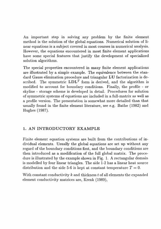
An important step in solving any problem by the finite element method is the solution of the global equations. Numerical solution of li­near equations is a subject covered in most courses in numerical analysis. However, the equations encountered in most finite element applications have some special features that justify the development of specialized solution algorithms.

The special properties encountered in many finite element applications are illustrated by a simple example. The equivalence between the stan­dard Gauss elimination procedure and triangular L U factorization is de­scribed. The symmetric LDLT form is derived, and the algorithm is modified to account for boundary conditions. Finally, the profile - or skyline - storage scheme is developed in detail. Procedures for solution of symmetric systems of equations are included in a full-matrix as well as a profile version. The presentation is somewhat more detailed than that usually found in the finite element literature, see e.g. Bathe (1982) and Hughes (1987).

1. AN INTRODUCTORY EXAMPLE

Finite element equation systems are built from the contributions of in­dividual elements. Usually the global equations are set up without any regard of the boundary conditions first, and the boundary conditions are then introduced as a modification of the full global matrix. The proce­dure is illustrated by the example shown in Fig. 1. A rectangular domain is modelled by four linear triangles. The side 1-2 has a linear heat source distribution and the side 5-6 is kept at constant temperature T = 0.

With constant conductivity k and thickness t of all elements the expanded element conductivity matrices are, Krenk (1989),

2

3 1 ql

® ® T=O h

0 CD 6 4 2

h h

Fig. 1. Heat conduction by triangular elements.

1 -1 0 0 0 0 -1 2 0 -1 0 0

lKn = kt 0 0 0 0 0 0 2 0 -1 0 1 0 0

0 0 0 0 0 0 0 0 0 0 0 0

1 0 -1 0 0 0 0 0 0 0 0 0

[Jqe] = kt -1 0 2 -1 0 0

2 0 0 - 1 1 0 0 0 0 0 0 0 0 0 0 0 0 0 0

0 0 0 0 0 0 0 0 0 0 0 0

[Kje] = kt 0 0 2 - 1 -1 0

2 0 0 -1 1 0 0 0 0 -1 0 1 0 0 0 0 0 0 0

0 0 0 0 0 0 0 0 0 0 0 0

(K:eJ = kt 0 0 0 0 0 0 2 0 0 0 1 0 -1

0 0 0 0 1 -1 0 0 0 -1 -1 2

After assembly the conductivity matrix is

4

(K] = L (K;eJ = ~t j=l

The load vector is

{!} = qlh 6

2 1 0 0 0 0

2 -1 -1 0 0 0

-1 -1 2 0 0 4

-1 -2 0 -1 0 0

0 0 -1 0 -2 -1 4 0 0 2 -1 -1

0 0 0

-1 -1 2

3

In addition there are unknown loads at nodes 5 and 6 in order to maintain the prescribed temperature along 5-6. The resulting equations are

2 - 1 -1 0 0 0 Tt 2 0 - 1 2 0 -1 0 0 T2 1 0

kt -1 0 4 -2 -1 0 T3 qlh 0 0 -0 -2 4 0 T4

= - + 0 2 -1 -1 6 0 0 0 -1 0 2 -1 Ts 0 Qs 0 0 0 -1 -1 2 Ts 0 Q6

4

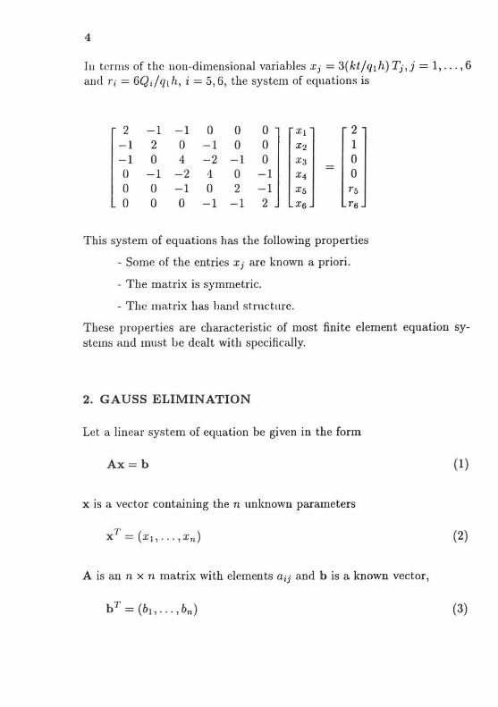
Iu terms of the non-dimensional variables xi = 3( kt / q1 h) Tj, j = 1, ... , 6 and r; = 6Qi/q 1 h, i = 5, 6, the system of equations is

2 -1 -1 0 0 0 XI 2 -1 2 0 -1 0 0 X2 1 -1 0 4 -2 -1 0 XJ 0

= 0 - 1 -2 4 0 -1 x4 0 0 0 -1 0 2 -1 xs rs 0 0 0 -1 -1 2 X6 T6

This system of equations has the following properties

- Some of the entries Xj are known a priori.

- The matrix is symmetric.

- The mat.rix has hand st.rnctme.

These properties are characteristic of most finite element equation sy­stems and must be dealt with specifically.

2. GAUSS ELIMINATION

Let a linear system of equation be given in the form

Ax=b (1)

x is a vector containing the n unknown parameters

xT = (xt, ... ,x,.) (2)

A is an n x n matrix with elements a;j and b is a known vector,

(3)

5

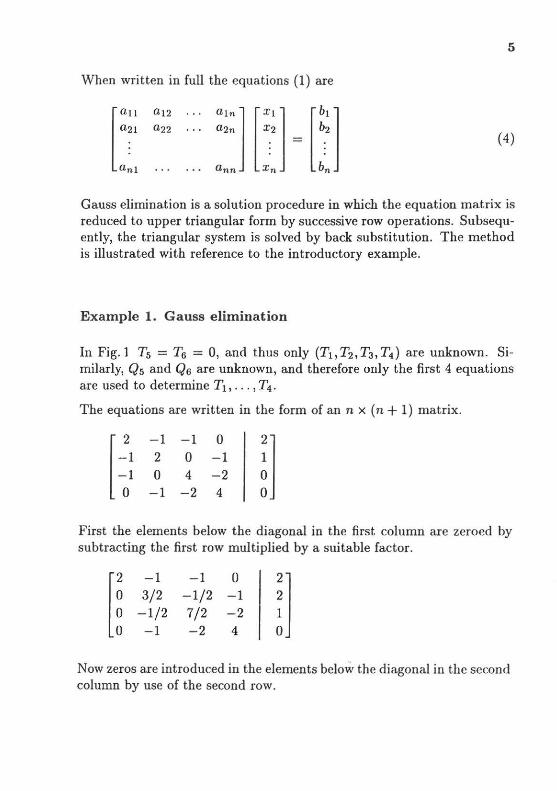
When written in full the equations (1) are

(4)

Gauss elimination is a solution procedure in which the equation matrix is reduced to upper triangular form by successive row operations. Subsequ­ently, the triangular system is solved by back substitution. The method is illustrated with reference to the introductory example.

Example 1. Gauss elimination

In Fig. 1 Ts = Ta = 0, and thus only (T1 , T2 , n, T4 ) are unknown. Si­milarly, Qs and Qa are unknown, and therefore only the first 4 equations are used to determine T1 , . .. , T4 .

The equations are written in the form of ann x (n + 1) matrix.

- 1 - 1 0 2 0 -1 0 4 - 2

- 1 - 2 4

First the elements below the diagonal in the first column are zeroed by subtracting the first row multiplied by a suitable factor.

[

2 - 1 0 3/2 0 -1/2 0 -1

- 1 0 -1/2 -1 7/2 - 2 - 2 4

Now zeros are introduced in the elements below the diagonal in the second column by use of the second row.

6

-1

-1/2 10/3 -7/3

0 -1

-7/3 10/3

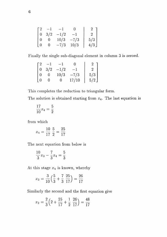
Finally the single sub-diagonal element in column 3 is zeroed.

[

2 -1 - 1

0 3/2 - 1/2 0 0 10/3 0 0 0

0 -1

-7/3 17/10

This completes the reduction to triangular form.

The solution is obtained starting from x 4 • The last equation is

17 5 - x4 =-10 2

from which

10 5 25 X<t = 17 2 = 17

The next equation from below is

10 7 5 -x3 - -x4 = -3 3 3

At this stage x4 is known, whereby

3 (5 7 25) 26 XJ = 10 3 + 3 17 = 17

Similarly the second and the first equation give

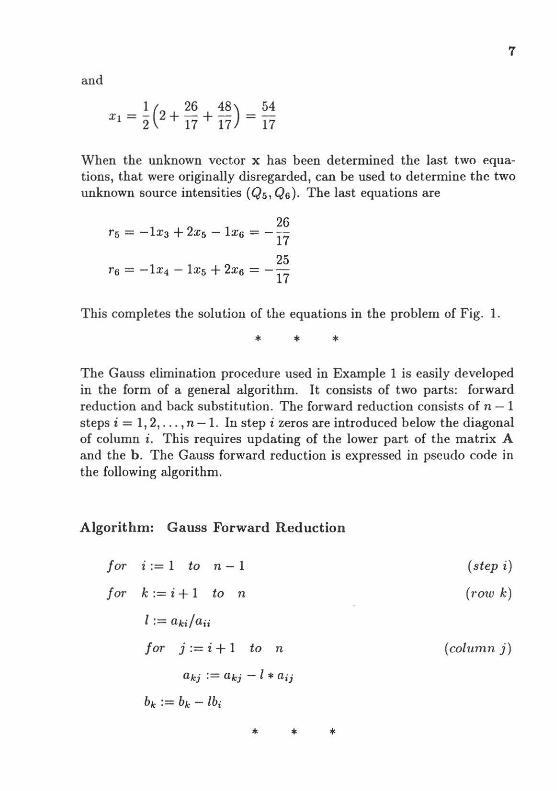
7

and

X l = ~ (2 + 26 + 48) = 54 2 17 17 17

When the unknown vector x has been determined the last two equa­tions, that were originally disregarded, can be used to determine the two unknown source intensities (Q5 , Q6 ). The last equations are

26 rs = - 1xa + 2xs - 1xs = -

17

25 rs = -1x4 -1xs +2xs = --

17

This completes the solution of the equations in the problem of Fig. 1.

* * * The Gauss elimination procedure used in Example 1 is easily developed in the form of a general algorithm. It consists of two parts: forward reduction and back substitution. The forward reduction consists of n- 1 steps i = 1, 2, ... , n -1. In step i zeros are introduced below the diagonal of column i. This requires updating of the lower part of the matrix A and the b . The Gauss forward reduction is expressed in pseudo code in the following algorithm.

Algorithm: Gauss Forward Reduction

for i := 1 to n - 1

f or k := i + 1 to n

for j := i + 1 to n

* * *

(step i)

(mw k)

(column j)

8

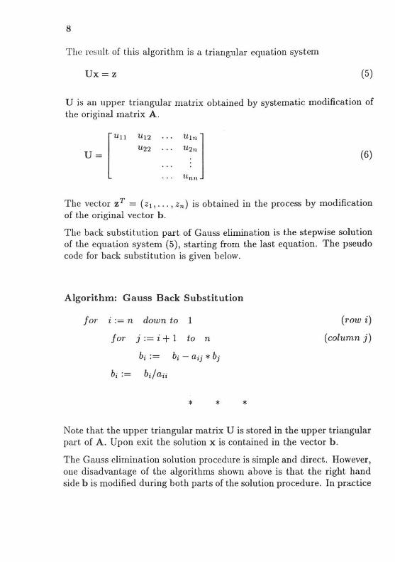
The result of this algorithm is a triangular equation system

Ux=z (5)

U is an upper triangular matrix obtained by systematic modification of the original matrix A.

[

UlJ

U = U!n 1 U2n

tt~, (6)

The vector z T = ( z1 , . .. , zn) is obtained in the process by modification of the original vector b .

The back substitution part of Gauss elimination is the stepwise solution of the equation system (5), starting from the last equation. The pseudo code for back substitution is given below.

Algorithm: Gauss Back Substitution

for i := n down to 1

for j := i + 1 to n

b; := b;- a;j * bj

b· ·-.. - b;j a;;

* * *

(row i)

(column j)

Note that the upper triangular matrix U is stored in the upper triangular part of A . Upon exit the solution x is contained in the vector b.

The Gauss elimination solution procedure is simple and direct. However, one disadvantage of the algorithms shown above is that the right hand side b is modified during both parts of the solution procedure. In practice

9

Gauss elimination is most often implemented in finite element programs in the form of matrix factorization.

Before proceeding it should be noticed that the forward reduction algo­rithm will break down, if a zero diagonal element a;; is encountered. In practice even a small diagonal element may cause problems with loss of accuracy. Such problems are usually countered by equilibration or pi­voting, see e.g. Press et al. {1986). Here the prime concern is with symmetric systems of equations, where these problems are not likely to arise. On the contrary any scaling or reordening of the equations may destroy the symmetry, and therefore only direct methods are dealt with here.

3. LU- FACTORlSATION

In the solution of linear equations it is often advantageous to separate the forward reduction part from the back substitution part. The result of the forward reduction was to produce a system of equations in the triangular form (5). This system was obtained by simultaneous modification of the matrix A and the right hand side b. It is demonstated below that this modification can be obtained by decomposing the matrix A into two factors L and U, where U is the upper triangular matrix (6), and L is a lower triangular matrix with unit diagonal elements.

J (7)

The factorisation amounts to determination of two triangular matrices L and U such that

A=LU

With this factorisation the equation system ( 1) takes the form

LUx=h

(8)

(9)

10

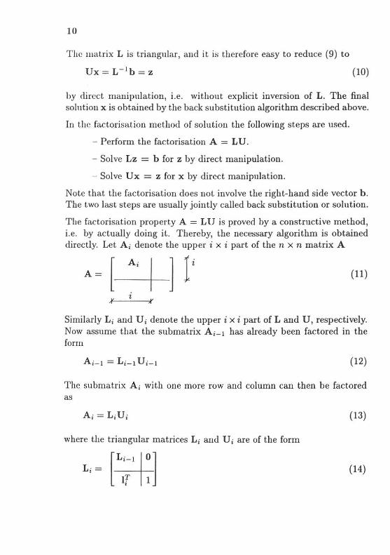
The matrix L is triangular, and it is therefore easy to reduce (9) to

(10)

by direct manipulation, i.e. without explicit inversion of L. The final solution xis obtained by the back substitution algorithm described above.

In the factorisation method of solution the following steps are used.

- Perform the factorisation A = L U .

- Solve Lz = b for z by direct manipulation.

- Solve Ux = z for x by direct manipulation.

Note that the factorisation does not involve the right-hand side vector b . The two last steps are usually jointly called back substitution or solution.

The factorisation property A = L U is proved by a constructive method, i.e. by actually doing it. Thereby, the necessary algorithm is obtained directly. Let A; denote the upper i x i part of the n x n matrix A

(11)

Similarly L; and U; denote the upper i x i part of L and U , respectively. Now assume that the submatrix A;_ 1 has already been factored in the form

(12)

The submatrix Ai with one more row and column can then be factored as

A; = L;U; (13)

where the triangular matrices L; and U; are of the form

L; ~ [L;;' I:] (14)

11

and

[

ui-1 u;] U;=

oT d; (15)

The proof follows from writing the matrix A; as

(16)

and then substituting L; and U; into (13). The result is

(17) d; + Ifu;

Comparison with (16) gives the following equation for the new i'th row If of L;, the new i'th column u; of U;, and the new diagonal element d; .

L;-1 u; =a; (18)

(19)

d; +If Uj = Cj (20)

The equations (18) and (19) for u; and I; are in lower triangular form, and can therefore be solved directly.

The three relations (18) - (20) comprise step i of the factorisation algo­rithm. In step i the factored part is increased in size from (i - 1) x (i -1) to i x i by adding a new row and column. Note that the new row and column do not change the parts, L;_1 and U;_ 1, that have already been factored. Thus only row i and column i are "active" in step i. This is

12

illw;tratcd in Fig. 2. The part A;_ 1 of the original matrix, correspon­ding to the factored part, is not needed in the further steps, and in most implementations L; and U; are written into the corresponding storage positions of A; as they are created. This is shown in the following LU factorisation algorithm.

1 Fig. 2. Progress of front in step i of L U-factorisation.

Algorithm: L U-factorisation.

for i := 2 to n

for j := 1 to i- 1

fo1· k := 1 to j - 1

* * *

}

(step i)

(eqn. j)

(uii from (18))

(l;i j1·om (19) )

(u;; from (20))

13

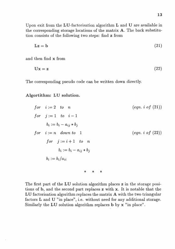
Upon exit from the LU-factorisation algorithm Land U are available in the corresponding storage locations of the matrix A. The back substitu­tion consists of the following two steps: find z from

Lz=b (21)

and then find x from

Ux=z (22)

The corresponding pseudo code can be written down directly.

Algortithm: L U solution.

for i := 2 to n (eqn. i of (21))

for j := 1 to i- 1

f or i := n down to 1 (eqn. i of {22))

for j := i + 1 to n

b; := b; - a;j * bj

b; := b;ja;;

* * *

The first part of the LU solution algorithm places z in the storage posi­tions of b, and the second part replaces z with x . It is notable that the LU factorisation algorithm replaces the matrix A with the two triangular factors L and U "in place", i.e. without need for any additional storage. Similarly the LU solution algorithm replaces b by x "in place".

14

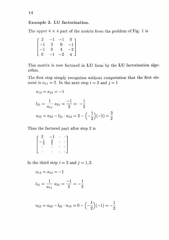
Example 2. L U factorisation.

The upper 4 x 4 part of the matrix from the problem of Fig. 1 is

- 1 2 0 -1

- 1 0 4

-2

~11 - 2 4

This matrix is now factored in L U form by the L U factorisation algo­rithm.

The first step simply recognizes without computation that the first ele­ment is ttu = 2. In the next step i = 2 and j = 1

1 -1 1 /21 = - a21 = - =

u11 2 2

tt22 = a22 -/2 1 · u12 = 2- ( -~)(-1) = ~

Thus the factored part after step 2 is

-1 3 2 1

In the third step i = 3 and j = 1, 2.

U JJ = a13 = - 1

1 - 1 1 l 3 1 =- a31 =- = --

u ll 2 2

15

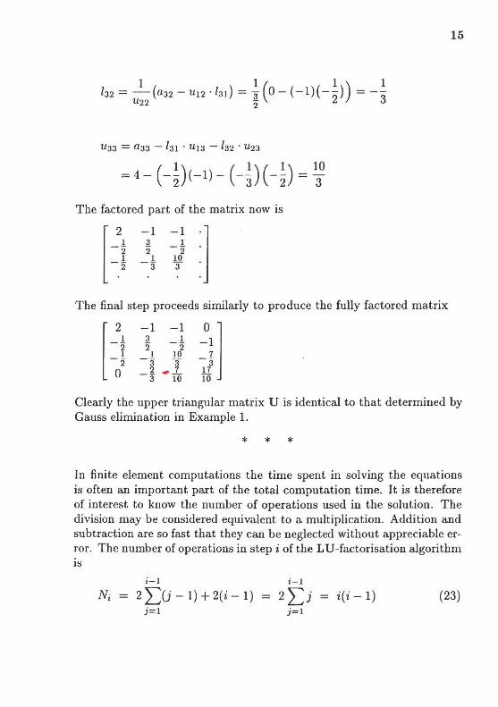
The factored part of the matrix now is

The final step proceeds similarly to produce the fully factored matrix

[ ~~ -1 -1 ;;] 3 1 2 -2

1 10 -3 3

2 ..,. .1_ 17 -3 10 10

Clearly the upper triangular matrix U is identical to that determined by Gauss elimination in Example 1.

* * *

In finite element computations the time spent in solving the equations is often an important part of the total computation time. It is therefore of interest to know the number of operations used in the solution. The division may be considered equivalent to a multiplication. Addition and subtraction are so fast that they can be neglected without appreciable er­ror. The number of operations in step i of the LU-factorisation algorithm IS

i-1 i - 1

N; = 2~)j-1)+2{i-1) = 2I> = i( i - 1) {23) j = l j=1

16

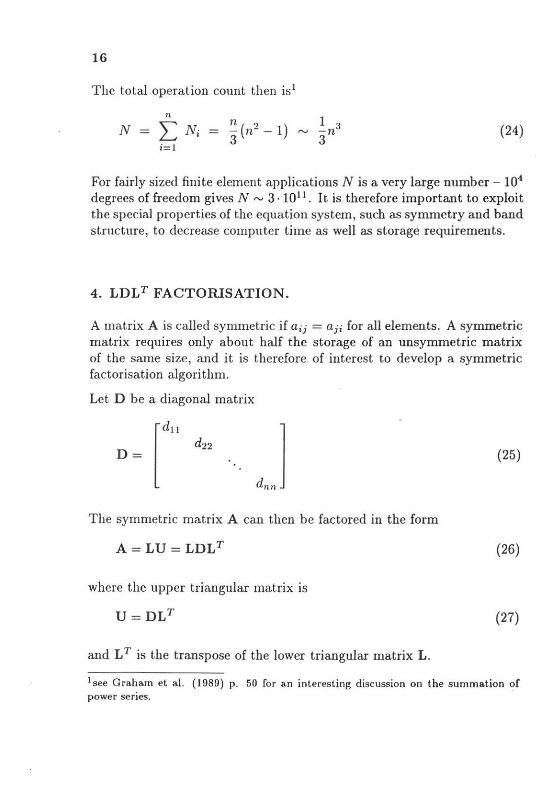
The total operation count then is 1

(24)

For fairly sized finite element applications N is a very large number - 104

degrees of freedom gives N"' 3 · 1011 . It is therefore important to exploit the special properties of the equation system, such as synunetry and band structure, to decrease computer time as well as storage requirements.

4. LDLT FACTORJSATION.

A matrix A is called symmetric if a ;j = aji for all elements. A symmetric matrix requires only about half the storage of an unsymmetric matrix of the same size, and it is therefore of interest to develop a synunetric factorisation algorithm.

Let D be a diagonal matrix

D= ldll

(25)

The symmetric matrix A can then be factored in the form

A = LU = LDLT (26)

where the upper triangular matrix is

(27)

and LT is the transpose of the lower triangular matrix L.

1 see Graham et al. (1989) p . 50 for an interesting discussion on the summation of power series.

17

A modified L U-factorisation algorithm for symmetric matrices can now be developed, in which only the lower triangular matrix L and the dia­gonal matrix D are computed and stored.

Write the submatrix A; in the form

The factored form

A;= L;D;Lf

contains the submatrices

and

D; = [ Di-1 I 0]. ~

Substitution of these expressions into (29) gives

Comparison with (28) gives the equations

(L;-lDi-I)li = a;

(28)

(29)

(30)

(31)

{32)

{33)

(34)

18

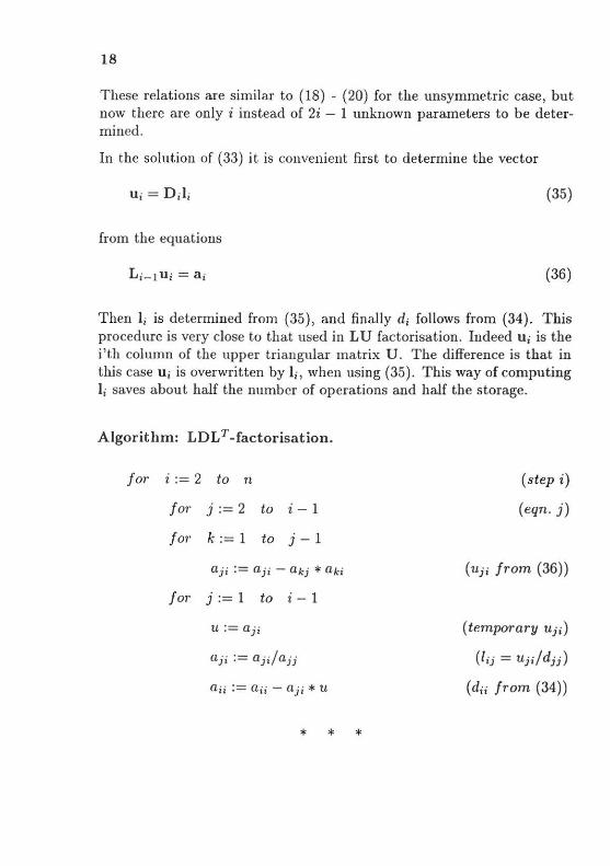
These relations are similar to {18) - {20) for the unsymmetric case, but now there are only i instead of 2i - 1 unknown parameters to be deter­mined.

In the solution of {33) it is convenient first to determine the vector

U; = D;l; {35)

from the equations

L;-lui =a; {36)

Then l; is determined from {35), and finally d; follows from {34). This procedure is very close to that used in LU factorisation. Indeed u; is the i'th column of the upper triangular matrix U. The difference is that in this case u; is overwritten by I;, when using (35). This way of computing l; saves about half the number of operations and half the storage.

Algorithm: LDLT -factorisation.

for i := 2 to n

fo1· j := 2 to i- 1

fm· k := 1 to j - 1

for j := 1 to i- 1

(step i)

(eqn. j)

(uji from (36))

u := aii (temporary Uj;)

a;;:=a;;-aii*U

* * *

(lij = Uj;jdjj)

(d;; from (34))

19

In the LDLT algorithm only the upper half of A is used, and upon exit this upper half has been replaced by LT and D . The algorithm works essentially "in place" with only a single temporary storage location needed. The operation count is

1 3 N,...., -n 6

about half of the L U algorithm.

The LDLT solution part has three phases

Lz = b

Dy = z

(37)

(38)

(39)

(40)

The implementation of the corresponding algorithm is straight forward, when it is remembered that LT, and not L, is stored in the locations of the matrix A .

Algorithm: LDLT solution.

for i := 2 to n

for j := 1 to i - 1

b; := b; - aj; * bj

for i := 1 to n

b; := b;fa;;

for. i := n- 1 down to 1

for j := i + 1 to n

b; := b; - a;j * bj

* * *

(z from (38))

(y from (39))

(x from ( 40))

20

Example 3. LDLT factorisation.

When the 4 x 4 matrix considered in Example 1 and 2 is factored by the LDLT algorithm, the upper half of A is replaced by D and LT. The result is

[2 1 1

!f j -2 -2 3 1 2 -3

10 3 10

17 10

This form should be compared with that obtained in Example 2.

* * *

5. PROFILE STORAGE ALGORITHM.

In finite element problems it is usually possible to obtain a banded structure of the equations by suitable numbering of the degrees of free­dom. Automatic procedures for optirnising the band structure have also been developed, see e.g. Schwarz (1988). The main point is illustrated in the following example.

Example 4. Bandwidth and profile.

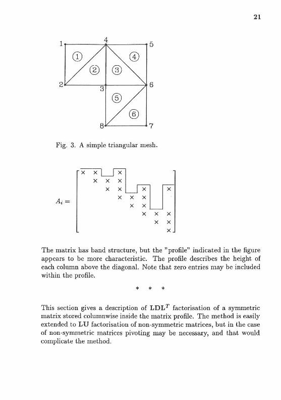
The element mesh in Fig. 3 is made up of simple triangles with linear interpolation. When the nodes are numbered as shown in the figure- this is not the optimal numbering - the upper half of the conductivity matrix has the entries.

1

2

Fig. 3.

A;=

4 5

@)

® 3

6

® ®

8 7

A simple triangular mesh.

X X X

X X X

X X

X

21

The matrix has band structure, but the "profile" indicated in the figure appears to be more characteristic. The profile describes the height of each column above the diagonal. Note that zero entries may be included within the profile.

* * *

This section gives a description of LDLT factorisation of a symmetric matrix stored colurnnwise inside the matrix profile. The method is easily extended to LU factorisation of non-symmetric matrices, but in the case of non-symmetric matrices pivoting may be necessary, and that would complicate the method.

22

The idea of profile storage of a symmetric matrix A and the corresponding LDLT factorisation algorithm follows from the relation (36),

L;_ 1u; = ai ( 41)

L;_ 1 is a lower triangular matrix, and it then follows that of the first i0 elements of a; are zero, then the first io elements of u; must also be zero. It follows from (35) that 1; also starts with i 0 zero elements. As a consequence of this the factored form of A given by D and LT fits within the profile of the original matrix A.

In profile storage of a matrix A the entries between the profile and the diagonal - including the diagonal - are stored columnwise in a one­dimensional array A;. The order of storage of the matrix of Example 4 is

1 2 6 3 4 7

5 8 12 18

A;= 9 10 13 19

(42) 11 14 20

15 16 21 17 22

23

The number of each diagonal element is stored in the index array

m;= (m1, m2, ... , mn) ( 43)

For the matrix ( 42) the index array m; is

1n; = (1,3,5,9,11,15,17,23) (44)

The index array determines the two-dimensional structure of the matrix completely. This column no. 6 starts with A(m5 + 1) = A(12) and ends with A(m6 ) = A(15).

23

Two modifications of the LDLT algorithm are needed, when profile stor­age is used:

- a correspondance between the double subscript of the algorithm and the single storage subscript must be established, and

- checks must be incorporated to prevent the algorithm from addres­sing locations outside the profile.

Let i 0 denote the number of zero elements above the profile in column No. i. The number of elements inside the profile is m;- mi-1· The total number of elements in column No. i is i, and thus

io = i- (m;- m;_t) (45)

For column No. 6 in ( 42)

io = 6- (15- 11) = 2

Similarly j 0 defines the number of zero elements in column No. j. io and j 0 serve as limits for any operation involving columns i and j.

The correspondance between elements in column i is

(46)

In the algorithm it is important to restrict the range of the subscript k to (io + 1, ... , i).

In the LDLT algorithm two columns, i and j, are in use simultaneously when forming products aki · aki, k = 1, ... , j - 1. Here the subscript k must start at max(jo, i 0 ) + 1. When these modifications are incorporated in the LDTT algorithm the following profile factorisation algorithm is obtained.

24

Algorithm: Profile factorisation.

f01· i := 2 to n

is:= m;- i

io := mi-1 -is

f or j := io + 2 to i- 1

Js := mj- j

]o := mj-1 - Js

ko := max (io,]o)

ji :=is+ j

for k := ko + 1 to j- 1

(sum index i)

(zeros in i)

(sum index j)

(zeros in j)

( max zeros i, j)

(index (j, i))

A(ji) := A(ji)- A(is + k) *A( is+ k)

for j := io + 1 to i- 1

ji :=is+ j

U := A(ji)

A(ji) := A(ji)/A(mj)

A(m;) := A(mi)- A(ji) * U

* * *

The profile solution procedure makes use of the same indexing scheme.

25

Algorithm: Profile solution.

for i := 2 to n

is := m; - i (sum index i)

i 0 := m;_ 1 -is (zeros in i)

for j := io + 1 to i- 1

b; := b; - A(is + j) * bj

for i := 1 to n

b; := b;fA(m;)

for i := n- 1 down to 1

for j := i + 1 to n

is:= mj- j

io := mi-1 - js

if i > jo then

b; := b;- A(js + i) * bj

* * *

(sum index j)

(zeroinj)

(profile)

In order to use the profile storage and solution scheme in a finite element calculation the index array m; must first be calculated by the program. This calculation is performed in two steps: first all elements are scanned and the array m; is used to accumulate the column heights, and finally the index values are calculated from the column heights. The accumulation of column heights is conveniently implemented as a dummy run of the assembly routine.

26

Algorithm: Get profile.

for i := 1 to n

m;:= 1

for k := 1 to Noof Elem

AssmElem (m;, ... ,k)

for i := 2 to n

m;:= mi-1 +m;

AssmElem(m;, ... , k):

n1 := fi1·st global DOF }

nNe := last global DOF

for i := 1 to Ne

Ne} for j := i + 1 to

h := In;- nj I +1

if n; < ni then

else

(initialize m;)

(get heights)

(height to index)

(find Ne global DOF)

(all combinations)

(new height)

if mn, < h then mn, := h

* * *

27

Example 5. Get profile.

Consider the example of Fig. 3. In this example n = 8 and the triangular elements have Ne = 3. First the array m; is initialized,

m;= (l,l,l,l,l,l,l,l)

The first call to AssrnElem concerns element k = 1 with global node references

n; = (1, 2, 4)

This leads to the update

m;= (1, 2, 1,4, 1, 1, 1, 1)

When all elements have been called the array m; contains the column heights,

m;= (1,2,2,4,2,4,2,6)

Finally sequential addition of column heights gives the index array

m; = (1 , 3, 5, 9, 11, 15, 17, 23)

This index array was already obtained directly from the matrix entries in ( 42).

* * *

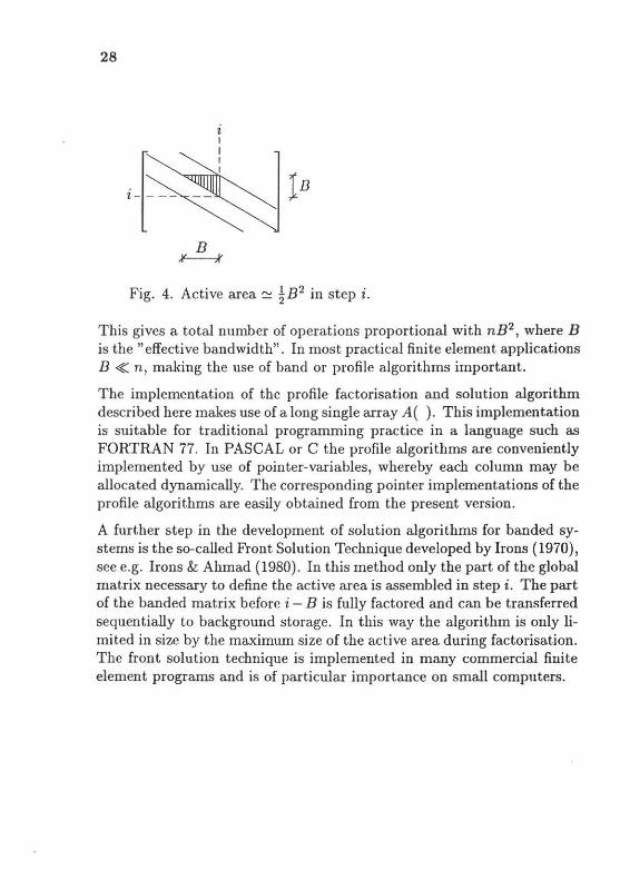
When the size of the inner loops of the factorisation algorithm are limited by the bandwidth or the profile the typical number of compu­tations in one step is approximately ~ B 2 as indicated in Fig. 4.

28

t I

i-[~ ]rn

Fig. 4. Active area~ ~B2 in step i.

This gives a total number of operations proportional with nB2 , where B is the "effective bandwidth". In most practical finite element applications B ~ n, making the use of band or profile algorithms important.

The implementation of the profile factorisation and solution algorithm described here makes use of a long single array A( ). This implementation is suitable for traditional programming practice in a language such as FORTRAN 77. In PASCAL or C the profile algorithms are conveniently implemented by use of pointer-variables, whereby each column may be allocated dynamically. The corresponding pointer implementations of the profile algorithms are easily obtained from the present version.

A further step in the development of solution algorithms for banded sy­stems is the so-called Front Solution Technique developed by Irons {1970), see e.g. Irons & Ahmad {1980). In this method only the part of the global matrix necessary to define the active area is assembled in step i. The part of the banded matrix before i - B is fully factored and can be transferred sequentially to background storage. In this way the algorithm is only li­mited in size by the maximum size of the active area during factorisation. The front solution technique is implemented in many commercial finite element programs and is of particular importance on small computers.

29

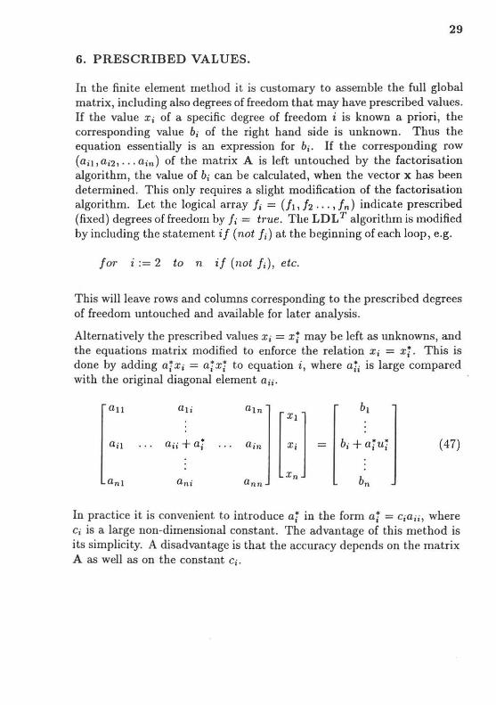
6. PRESCRIBED VALUES.

In the finite element method it is customary to assemble the full global matrix, including also degrees of freedom that may have prescribed values. If the value x; of a specific degree of freedom i is known a priori, the corresponding value b; of the right hand side is unknown. Thus the equation essentially is an expression for b;. If the corresponding row (a;1 , a;2 , ... a;n) of the matrix A is left untouched by the factorisation algorithm, the value of b; can be calculated, when the vector x has been determined. This only requires a slight modification of the factorisation algorithm. Let the logical array J; = (ft, h ... , fn) indicate prescribed (fixed) degrees of freedom by J; = t1·ue. The LDLT algorithm is modified by including the statement if (not J;) at the beginning of each loop, e.g.

for i := 2 to n if (not/;), etc.

This will leave rows and columns corresponding to the prescribed degrees of freedom untouched and available for later analysis.

Alternatively the prescribed values x; = xi may be left as unknowns, and the equations matrix modified to enforce the relation x; = x;. This is done by adding a;x; = a;x; to equation i, where a;; is large compared with the original diagonal element a;;.

au a1; a1n

[] bt

a;1 a;; +a; a;n = b; + atui (47)

anl ani ann bn

In practice it is convenient to introduce a; in the form ai = c;a;;, where c; is a large non-dimensional constant. The advantage of this method is its simplicity. A disadvantage is that the accuracy depends on the matrix A as well as on the constant c;.

30

REFERENCES.

Bathe, K.-J. (1982): Finite Element Procedures in Engineering Analysis. Prentice- Hall, Englewood Cliffs.

Graham, R. 1., Knut.h, D. E. and Pata.shnik, 0. (1989): Concrete Mat­hematics. Addison-Wesley, Reading, Mass.

Hughes, J. R. H. (1987): The Finite Element Method. Prentice-Hall, Englewood Cliffs.

Irons, B. (1970): A frontal solution program for finite element analysis. International Journal for Numerical Methods in Engineering. 2 , pp. 5-32.

Irons, B. and Ahmed, S. (1980): Techniq·ues of Finite Elements. Ellis Horwood, Chichester.

Krenk, S. (1989): Simple trekantelementer. Department of Building Te­chnology and Structural Engineering, University of Aalborg.

Press, W. H., Flannery, B. P., Teukolsky, S. A. and Vetterling, W. T . (1986): Numerical Recipes. Cambridge University Press, Cambridge.

Schwarz, H. R. (1988): Finite Element Methods. Academic Press, Lon­don.