Aalborg Universitet

Slowly-varying 2. order Wave Forces on Large Structures

Brorsen, Michael

Publication date:2006

Document VersionPublisher's PDF, also known as Version of record

Link to publication from Aalborg University

Citation for published version (APA):Brorsen, M. (2006). Slowly-varying 2. order Wave Forces on Large Structures. Aalborg: Department of CivilEngineering, Aalborg University. (DCE Lecture Notes; No. 1).

General rightsCopyright and moral rights for the publications made accessible in the public portal are retained by the authors and/or other copyright ownersand it is a condition of accessing publications that users recognise and abide by the legal requirements associated with these rights.

? Users may download and print one copy of any publication from the public portal for the purpose of private study or research. ? You may not further distribute the material or use it for any profit-making activity or commercial gain ? You may freely distribute the URL identifying the publication in the public portal ?

Take down policyIf you believe that this document breaches copyright please contact us at vbn@aub.aau.dk providing details, and we will remove access tothe work immediately and investigate your claim.

Downloaded from vbn.aau.dk on: April 29, 2017

Slowly-varying 2. order Wave Forceson Large Structures

Michael Brorsen

ISSN 1901-7286DCE Lecture Notes No. 1 Department of Civil Engineering

Aalborg University

Department of Civil Engineering

Water and Soil

DCE Lecture Notes No. 1

Slowly-varying 2. order Wave Forces on LargeStructures

by

Michael Brorsen

July 2006

c© Aalborg University

Scientific Publications at the Department of Civil Engineering

Technical Reports are published for timely dissemination of research resultsand scientific work carried out at the Department of Civil Engineering (DCE) atAalborg University. This medium allows publication of more detailed explanationsand results than typically allowed in scientific journals.

Technical Memoranda are produced to enable the preliminary disseminationof scientific work by the personnel of the DCE where such release is deemed to beappropriate. Documents of this kind may be incomplete or temporary versions ofpapers-or part of continuing work. This should be kept in mind when referencesare given to publications of this kind.

Contract Reports are produced to report scientific work carried out undercontract. Publications of this kind contain confidential matter and are reserved forthe sponsors and the DCE. Therefore, Contract Reports are generally not availablefor public circulation.

Lecture Notes contain material produced by the lecturers at the DCE foreducational purposes. This may be scientific notes, lecture books, exampleproblems or manuals for laboratory work, or computer programs developed at theDCE.

Theses are monograms or collections of papers published to report the scientificwork carried out at the DCE to obtain a degree as either PhD or Doctor ofTechnology. The thesis is publicly available after the defence of the degree.

Latest News is published to enable rapid communication of information aboutscientific work carried out at the DCE. This includes the status of researchprojects, developments in the laboratories, information about collaborative workand recent research results.

Published 2006 byAalborg UniversityDepartment of Civil EngineeringSohngaardsholmsvej 57,DK-9000 Aalborg, Denmark

Printed in Denmark at Aalborg University

ISSN 1901-7286 DCE Lecture Notes No. 1

Contents

1 Drift forces 1

1.1 Introduction . . . . . . . . . . . . . . . . . . . . . . . . . . . . . . . . 1

1.2 Physical reasons for drift forces . . . . . . . . . . . . . . . . . . . . . 2

2 Drift forces from regular waves 4

2.1 Time average of the momentum equation . . . . . . . . . . . . . . . . 4

2.2 Wave thrust . . . . . . . . . . . . . . . . . . . . . . . . . . . . . . . . 6

2.3 Momentum in regular waves on deep water . . . . . . . . . . . . . . . 10

2.4 Deep water. Constant drift force on a body totally absorbing theincident wave energy . . . . . . . . . . . . . . . . . . . . . . . . . . . 12

2.5 Deep water. Constant drift force on a body totally reflecting theincident wave energy . . . . . . . . . . . . . . . . . . . . . . . . . . . 13

2.6 Finite water depth. Generalized expression of the constant drift forceon a floating body . . . . . . . . . . . . . . . . . . . . . . . . . . . . 14

2.7 Constant drift force on a 3-D body in regular waves. . . . . . . . . . . 14

3 Drift forces from irregular waves 15

3.1 Approximate calculation of a slowly varying drift force . . . . . . . . 15

3.2 Bounded long waves in irregular waves . . . . . . . . . . . . . . . . . 15

3.3 Principal structure of the expression for drift forces in irregular waves 20

3.4 Newman’s approximation . . . . . . . . . . . . . . . . . . . . . . . . . 23

3.5 Calculation of the slowly-varying drift force by use of the BoundaryElement Method . . . . . . . . . . . . . . . . . . . . . . . . . . . . . 25

4 References 26

i

1 Drift forces

1.1 Introduction

The average over time of 1. order wave loads on a structure is always equal tozero. This is due to the fact that all load components are determined by 1. orderwave theory and the integration of all wave loads stops at mean water level(MWL) i.e. the average over one wave period of the surface level. Thiscorresponds to assuming a constant submerged area of the body and when theload averaged over time is zero at all points, the total load is of course also zero.

In reality, however, the wave loads are non-linear and the may be separated intothe following 3 components:

1) forces at frequencies, fforce , equal to the wave frequencies fw ∼ 1/Tp, whereTp is the peak-period in the wave spectrum. The order of magnitude of theseforces is o(H/L), where H is the wave height and L is the wave length.

2) a constant drift force, defined as the average over a long time span of thewave forces. The order of magnitude is o((H/L)2).

3) slowly-varying drift forces, which may be determined from the total waveloads by filtering with a filter allowing only low frequent signals to pass.Typically the loads have frequencies in the range

1

10fw < fforce <

1

5fw (1)

The order of magnitude the slowly-varying drift forces is o((H/L)2).

In the following the non-linear drift forces are considered. Basically one wouldassume that the drift forces are of minor importance because they are smallcompared to the forces at wave frequencies. In practice, however, drift forces are ofmajor importance for the motions of a floating body.

The combination of large masses and relative small spring forces (for example inslack moorings) results in natural (resonance) periods with an order of magnitudeof one minute, and such periods are often coinciding with the periods of driftforces as indicated above.

This may result in resonance and because the damping is quite limited for shipmotions at these frequencies, it may results in large motions with correspondinglarge mooring forces.

1

1.2 Physical reasons for drift forces

When a body with relatively large dimensions compared to the wave length isconsidered, it may be shown that the viscous forces are of marginal importance.The vorticity created in the boundary layer has in this case only marginal effect onthe flow field outside the thin layer. With good approximation the flow field canbe considered free of vorticity and consequently potential theory can be applied,where the relation between particle velocity, ~v, and the velocity potential, ϕ, is:

~v = gradϕ = ∇ϕ (2)

Furthermore, it is a very good approximation to consider the forces from the wateras pressure forces, i.e. locally acting in a direction perpendicular to the surface ofthe body.

The total non-stationary force on the body can therefore be determined from:

~F (t) =∫

Ap~n dA (3)

where

A = A(t) is the submerged area of the body

~n = ~n(t) is the normal to the body surface, positive from water towards the body.Varies in time, if the body moves.

The pressure, p, is calculated by Bernoulli’s generalised equation :

p = −ρ g z − ρ∂ϕ

∂t− 1

2ρ v2 (4)

The horizontal components of the drift force, which usually are the mostinteresting, may be determined by projecting the drift force on the horizontalx-axis:

Fx(t) =∫

Ap nx dA (5)

The average of Fx(t) over one wave period T is:

Fx =1

T

∫ T

0Fx(t)dt 6= 0 (6)

where the symbol above a variable means average over time.

Several reasons leads to Fx 6= 0, but the two major reasons are:

1) the pressure forces act up to the instantaneous position of free surface andnot to MWL

2

2) the non-linear term −12ρ v2 in Bernoullis equation, due to v2 > 0.

As analytical solutions do not exist to non-linear problems, one must applynumerical methods to calculate drift forces.

If it is possible to calculate the non-linear flow close to the structure equation (3)may be used to calculate the drift force. The result is called a near-field solution.

Formerly it was impossible to obtain near-field solutions in the time domain due tolack of computer power. Instead solutions based on the momentum equation weredeveloped. These solutions only require information on the flow field far from thestructure. Accordingly they are called far-field solutions.

To day a near-field solution can be obtained, but it requires much larger computerpower than a far-field solution. The pay off from this extra effort is time series ofboth local and total forces in contrast to the time average of the total force, whichis the only result produced by a far-field solution.

3

2 Drift forces from regular waves

Under special conditions drift forces may be calculated approximately by means of1. order theory, only by including the 2. order components, i.e. components withthe order of magnitude o((H/L)2. By the way, in many textbooks this method isapplied to derive the expression for the energy transport velocity.

2.1 Time average of the momentum equation

Below is shown that the the average over one wave period of the momentumequation may be considered as a force equilibrium equation.

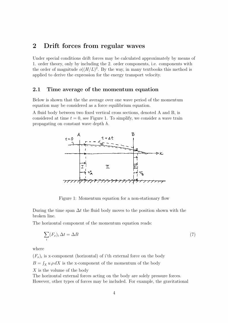
A fluid body between two fixed vertical cross sections, denoted A and B, isconsidered at time t = 0, see Figure 1. To simplify, we consider a wave trainpropagating on constant wave depth h.

Figure 1: Momentum equation for a non-stationary flow

During the time span ∆t the fluid body moves to the position shown with thebroken line.

The horizontal component of the momentum equation reads:

∑

i

(Fx)i ∆t = ∆B (7)

where

(Fx)i is x-component (horizontal) of i’th external force on the body

B =∫X u ρ dX is the x-component of the momentum of the body

X is the volume of the bodyThe horizontal external forces acting on the body are solely pressure forces.However, other types of forces may be included. For example, the gravitational

4

forces should be included when non-horizontal components of the momentumequation are considered.

The change in momentum may be determined in this way:

∆B = B(∆t)−B(0)

= B(∆t)II + B(∆t)III + B(∆t)IV −B(0)I −B(0)II (8)

where the indices I, II, III og IV refer to the volumes indicated on Figure 1 1.

As B(0)IV = 0, we may reformulate equation (8) to:

∆B = B(∆t)II −B(0)II + B(∆t)IV −B(0)IV + B(∆t)III −B(0)I

=∂(BII + BIV )

∂t∆t +

∑

B

(ρ vB ∆t ∆z) vB −∑

A

(ρ vA ∆t ∆z) vA

=∂(BII + BIV )

∂t∆t +

∫

Bρ vB ∆t vB dz −

∫

Aρ vA ∆t vA dz (9)

Note that the size of volume II is finite, and the volume of I is going towards zerofor ∆t → 0. We therefore only make a small error (which can be made arbitrarilysmall) by using the approximation

∂(BII + BIV )

∂t=

∂BAB

∂t

Consequently the momentum equation, equation (7), reads:

∑

i

(Fx)i ∆t =∂BAB

∂t∆t + ∆t

(∫

Bρ v2

B dz −∫

Aρ v2

A dz)

(10)

After division by ∆t we obtain

∑

i

(Fx)i =∂BAB

∂t+

∫

Bρ v2

B dz −∫

Aρ v2

A dz (11)

Because the integrals in equation (11) have the dimension force (even though theyrepresent changes of momentum) they are called inertia forces.

In the following these forces are denoted I in accordance with the general practicewithin hydraulics. If the expressions

IA =∫

Aρv2

Adz (12)

5

IB =∫

Bρv2

Bdz (13)

are used for substitution into equation (11) and the equation subsequently areaveraged over one wave period, the average of the momentum equation reads

∑

i

(Fx)i =1

T

∫ T

0

∂BAB

∂tdt + IB − IA (14)

The integral in equation (14) may be reformulated to∫ T

0

∂BAB

∂tdt =

∫ T

0d (BAB) = |BAB|T0 = BAB(T )−BAB(0) = 0 (15)

due to the fact that a body between two fixed cross section has the samemomentum at time t = 0 and time t = T .

Consequently the time average of the momentum equation reads

∑

i

(Fx)i + IA − IB = 0 (16)

Equation (16) shows that formally there exists equilibrium between all horizontalforces averaged over one wave period. The momentum equation for a body instationary flow can be interpreted the same way, but time averaging is of coursenot necessary.

Therefore a vertical cross section is exposed to the sum of the time averagedpressure force an the time averaged inertia force, when the time averagedmomentum equation is applied as a force equilibrium equation.

2.2 Wave thrust

In a wave motion a vertical cross section is exposed by the following time averagedforce:

F = P + I (17)

where

P =1

T

∫ T

0P dt

=1

T

∫ T

0

(∫ η

−hp dz

)dt

=1

T

∫ T

0

(∫ η

−h(phyd + p+)dz

)dt

=1

T

∫ T

0

(∫ η

−h(ρ g (−z) + p+)dz

)dt (18)

6

og

I =1

T

∫ T

0I dt

=1

T

∫ T

0

(∫ η

−hρ v2 dz

)dt (19)

where z is the level, i.e. the vertical distance above a datum. The datum may bechosen arbitrarily.

If only progressive waves are considered, the integrals in the equations (18) andequation (19) may be solved analytically, see for example Jonsson & Svendsen(1980) and Fredsøe (1990).

The expression for the force, P0, corresponding to hydrostatic pressure, phyd, reads:

P0 =∫ 0

−hphyd dz =

∫ 0

−hρ g (−z)dz =

1

2ρ g h2 (20)

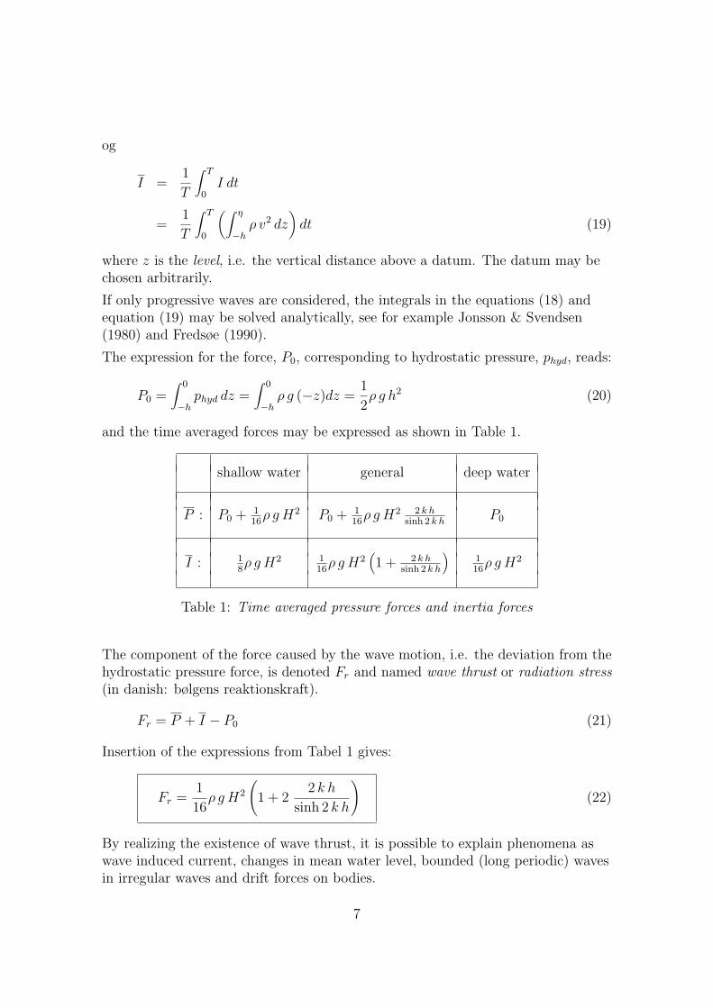
and the time averaged forces may be expressed as shown in Table 1.

shallow water general deep water

P : P0 + 116

ρ g H2 P0 + 116

ρ g H2 2 k hsinh 2 k h

P0

I : 18ρ g H2 1

16ρ g H2

(1 + 2 k h

sinh 2 k h

)116

ρ g H2

Table 1: Time averaged pressure forces and inertia forces

The component of the force caused by the wave motion, i.e. the deviation from thehydrostatic pressure force, is denoted Fr and named wave thrust or radiation stress(in danish: bølgens reaktionskraft).

Fr = P + I − P0 (21)

Insertion of the expressions from Tabel 1 gives:

Fr =1

16ρ g H2

(1 + 2

2 k h

sinh 2 k h

)(22)

By realizing the existence of wave thrust, it is possible to explain phenomena aswave induced current, changes in mean water level, bounded (long periodic) wavesin irregular waves and drift forces on bodies.

7

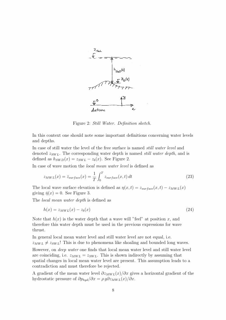
Figure 2: Still Water. Definition sketch.

In this context one should note some important definitions concerning water levelsand depths.

In case of still water the level of the free surface is named still water level anddenoted zSWL. The corresponding water depth is named still water depth, and isdefined as hSWD(x) = zSWL − zb(x). See Figure 2.

In case of wave motion the local mean water level is defined as

zMWL(x) = z̄surface(x) =1

T

∫ T

0zsurface(x, t) dt (23)

The local wave surface elevation is defined as η(x, t) = zsurface(x, t)− zMWL(x)giving η̄(x) = 0. See Figure 3.

The local mean water depth is defined as

h(x) = zMWL(x)− zb(x) (24)

Note that h(x) is the water depth that a wave will ”feel” at position x, andtherefore this water depth must be used in the previous expressions for wavethrust.

In general local mean water level and still water level are not equal, i.e.zMWL 6= zSWL! This is due to phenomena like shoaling and bounded long waves.

However, on deep water one finds that local mean water level and still water levelare coinciding, i.e. zMWL = zSWL. This is shown indirectly by assuming thatspatial changes in local mean water level are present. This assumption leads to acontradiction and must therefore be rejected.

A gradient of the mean water level ∂zMWL(x)/∂x gives a horizontal gradient of thehydrostatic pressure of ∂phyd/∂x = ρ g∂zMWL(x)/∂x.

8

Figure 3: Wave motion. Definition sketch.

This pressure gradient gives a non-zero resulting hydrostatic pressure force on abody. The size of this pressure force reads:

Phyd = −∫

Xgrad phyd dX

= −∫

Xρ g

∂zMWL

∂xdX

= −ρ g∂zMWL

∂x

∫

XdX , as the gradient is constant along a vertical

= −ρ g∂(zMWL)

∂xhA , as the volume reads X = hA

As Phyd →∞ for h →∞, it is obvious that changes in the local mean water levelcan not be present at deep water, because there exist no other wave induced forceswhich could out balance Phyd in the momentum equation.

9

2.3 Momentum in regular waves on deep water

Regular waves have a non-zero mean value of the momentum in the direction ofpropagation, though this momentum is of 2. order, i.e. the order of magnitude iso((H/L)2).

This mean momentum is due to a greater volume (with positive velocities) underthe wave crest than the volume (with negative velocities) under the wave trough.

In practice the mean momentum reads

< B > =1

L

∫ L

0B(x) dx

or

< B > =1

L

∫ L

0

(∫ η

−hρ u dz

)dx (25)

It is by no means trivial to determine < B > from this integral for finite waterdepths.

On deep water it is simpler as shown below. We consider 1. order waves with thesurface elevation

η =H

2cos(ωt− kx) (26)

and horizontal particle velocities:

u =π H

T

cosh k(z + h)

sinh khcos(ωt− kx) (27)

Without loss of generality the momentum B(x) is calculated at the time t = 0.The horizontal momentum pr. unit length (along the wave front) is:

B(x) =∫ η

−hρ u(z) dz

=∫ η

−hρ

π H

T

cosh k(z + h)

sinh khcos kx dz

=ρ π H

T· cos kx

sinh kh

∫ η

−hcosh k(z + h) dz

=ρ π H

T· cos kx

sinh kh· 1

k

∫ η

−hcosh k(z + h) d(k(z + h))

=ρ π H

T· cos kx

sinh kh· 1

k|sinh k(z + h)|η−h

10

B(x) =ρ π H

T· cos kx

sinh kh· 1

ksinh k(η + h)

=ρ L H

2 T· sinh k(η + h)

sinh khcos kx

On deep water the following is valid:

sinh k(η + h)

sinh kh≈ ek(η+h)

ekh= ekη ≈ 1 + k η

After insertion of this expression and the expression for η, the equation for B(x)reads

B(x) =ρ L H

2 T

(1 + k

H

2cos kx

)cos kx

This expression is substituted into equation (25) giving:

< B > =ρH

2 T

∫ L

0

(cos kx + k

H

2cos2 kx

)dx

=ρH

2 T· k H

2· L

2

=1

2ρ a2 k c

where a = H/2 and c = L/T .

On deep water one has

c2 =g

kand cg = c

where cg is the energy transport velocty. The equation for mean momentum ondeep water therefore reads:

< B >=1

2ρ g a2 1

c=

1

4ρ g a2 1

cg

(28)

11

2.4 Deep water. Constant drift force on a body totallyabsorbing the incident wave energy

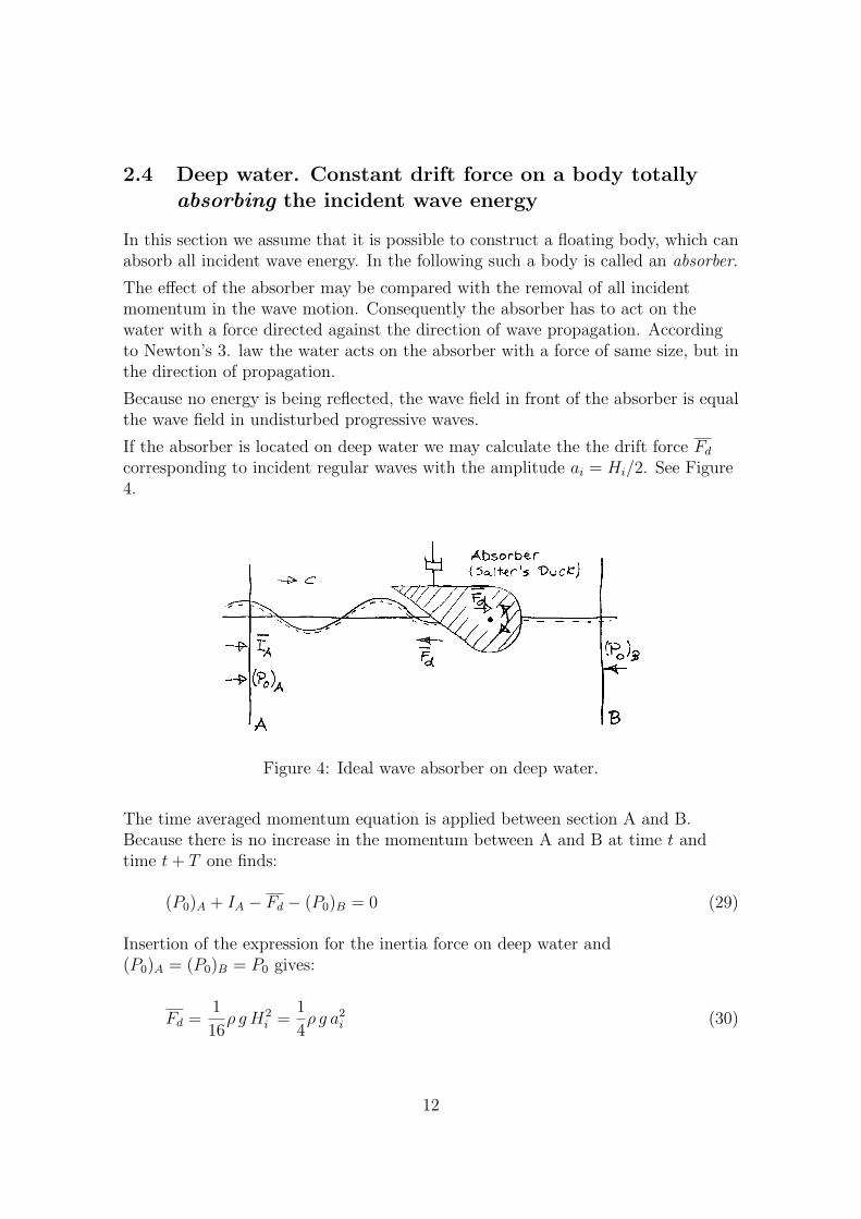
In this section we assume that it is possible to construct a floating body, which canabsorb all incident wave energy. In the following such a body is called an absorber.

The effect of the absorber may be compared with the removal of all incidentmomentum in the wave motion. Consequently the absorber has to act on thewater with a force directed against the direction of wave propagation. Accordingto Newton’s 3. law the water acts on the absorber with a force of same size, but inthe direction of propagation.

Because no energy is being reflected, the wave field in front of the absorber is equalthe wave field in undisturbed progressive waves.

If the absorber is located on deep water we may calculate the the drift force Fd

corresponding to incident regular waves with the amplitude ai = Hi/2. See Figure4.

Figure 4: Ideal wave absorber on deep water.

The time averaged momentum equation is applied between section A and B.Because there is no increase in the momentum between A and B at time t andtime t + T one finds:

(P0)A + IA − Fd − (P0)B = 0 (29)

Insertion of the expression for the inertia force on deep water and(P0)A = (P0)B = P0 gives:

Fd =1

16ρ g H2

i =1

4ρ g a2

i (30)

12

fully reflecting body

standing wave

Figure 5: Deep water. Body reflects incident waves totally.

2.5 Deep water. Constant drift force on a body totallyreflecting the incident wave energy

In this section we assume that the size of the floating body is so large that allincident wave energy is being reflected. Therefore standing waves are created infront of the absorber. See Figure 5.

If the body is located on deep water the drift force Fd may be calculated byarguments from analogy. The amplitude of the regular incident waves is againai = Hi/2.

In case of full reflection of the waves the body has to:

1) absorb the incident waves

2) generate similar waves moving in the opposite direction

The effect of 1) has been calculated at section 2.4. The reflected waves containsthe same size of momentum but in opposite direction. The same mean force musttherefore act on the water no matter if waves are absorbed or generated.Accordingly the necessary mean force acting on the water from the body is twiceas large as the force necessary to absorb waves totally. The drift force on the bodyat complete reflection is therefore

Fd = 2 · 1

16ρ g H2

i =1

2ρ g a2

i (31)

In this case the amplitude of the reflected waves is ar = ai, and we mayreformulate equation (31) to

Fd =1

2ρ g a2

r (32)

In the literature this equation is often called Maruo’s equation.

13

2.6 Finite water depth. Generalized expression of theconstant drift force on a floating body

In general the size of the body is not large enough to cause complete reflection ofthe waves. Part of the incident energy normally passes under the body and thisenergy is called transmitted wave energy. The amplitude of the transmitted wavesis denoted at.

The amount of transmitted energy increases if the floating body is allowed to move.The body is so to speak more transparent to the waves when it can move freely.

For linear 2-D waves on finite water depth, Longuet-Higgins (1977) has shown thaton a long, floating body the drift force pr. m may by determined from:

Fd =1

4ρ g (a2

i + a2r − a2

t )

(1 +

2 k h

sinh 2 k h

)(33)

where at is the amplitude of the transmitted waves.

Equation (33) is a generalized version of Maruo’s equation, but the derivation is byno means trivial. This is due to gradients of the local mean water levels caused bychanges in local wave height.

Note that an increase of the wave height causes an increase of the wave thrust.Because the time averaged momentum equation corresponds to a force equilibrium,there has to occur a reduction in the hydrostatic pressure force when the waveheight increases. This is only possible by a change in the local mean water level.

2.7 Constant drift force on a 3-D body in regular waves.

So far only drift forces on infinite long bodies has been treated. In these caseswave energy may only be transmitted under the body. When the length of thebody is finite, wave energy may also be transmitted around the ends of the body,and the body is called a 3-D body.

Accordingly, diffraction are of importance, and even far-field solutions require thatthe wave field around the body at least is calculated by numerical methods basedon 1. order wave theory.

It is out of the scope of this note to describe such calculations in details, and inthe following we will simply assume that we are capable of calculating the constantdrift force on a 3-D body with arbitrary shape.

14

force

elevation

time

time

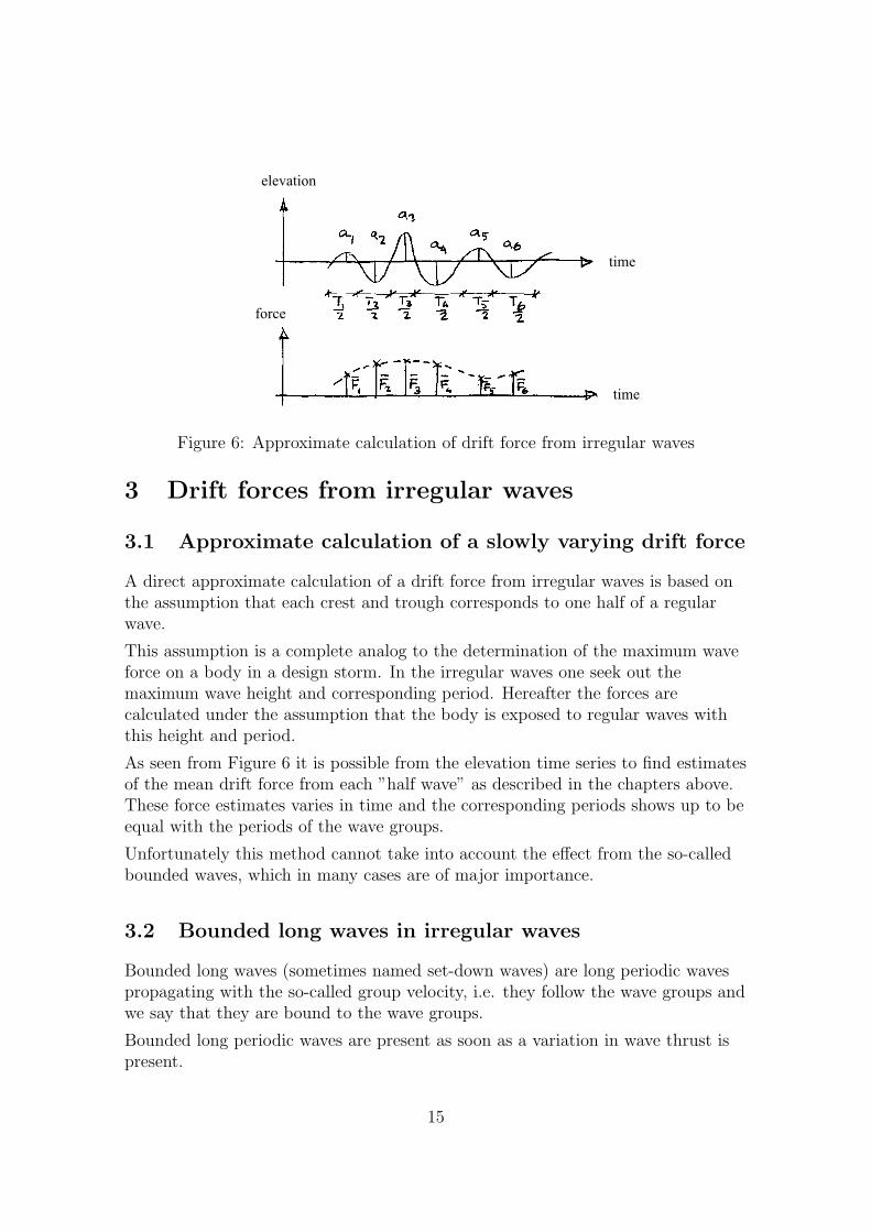
Figure 6: Approximate calculation of drift force from irregular waves

3 Drift forces from irregular waves

3.1 Approximate calculation of a slowly varying drift force

A direct approximate calculation of a drift force from irregular waves is based onthe assumption that each crest and trough corresponds to one half of a regularwave.

This assumption is a complete analog to the determination of the maximum waveforce on a body in a design storm. In the irregular waves one seek out themaximum wave height and corresponding period. Hereafter the forces arecalculated under the assumption that the body is exposed to regular waves withthis height and period.

As seen from Figure 6 it is possible from the elevation time series to find estimatesof the mean drift force from each ”half wave” as described in the chapters above.These force estimates varies in time and the corresponding periods shows up to beequal with the periods of the wave groups.

Unfortunately this method cannot take into account the effect from the so-calledbounded waves, which in many cases are of major importance.

3.2 Bounded long waves in irregular waves

Bounded long waves (sometimes named set-down waves) are long periodic wavespropagating with the so-called group velocity, i.e. they follow the wave groups andwe say that they are bound to the wave groups.

Bounded long periodic waves are present as soon as a variation in wave thrust ispresent.

15

Wave thrust is proportional to the square of the wave height in regular waves. Agradient in wave height therefore gives a gradient in the wave thrust and accordingto the time averaged momentum equation this thrust gradient has to be balancedby a gradient in the hydrostatic pressure force. This is only possible if a gradientof the local mean level exists, i.e. the mean water level is sloping.

If the wave height in a wave group varies slowly in space, the waves may locally beconsidered as regular waves, and the previous expressions for wave thrust inregular waves may be applied.

For wave groups we should therefore expect the local mean water level to behighest under small waves (group nodes) and lowest under the highest waves(between the nodes). Consequently a long wave is created having a length equal tothe length of the wave groups. It is obvious that this long wave must propagatewith the same velocity as the wave groups do. This leads to the name boundedwaves.

The most ordinary wave groups may be formed by super position of two regularwaves having periods fairly close to each other. This wave condition is namedregular wave groups or pair of beating waves.

For simplicity we consider first wave groups formed by super position of tworegular waves having the same amplitude. The expressions for these regular wavesηn and ηm reads:

ηn = a cos(ωn t− kn x) og ηm = a cos(ωm t− km x) (34)

It is assumed that the periods are close to each other with

Tn < Tm ⇔ ωn > ωm

giving

Ln < Lm ⇔ kn > km

as L increases monotonic with T .

By means of trigonometric relations the resulting surface elevation ηs reads:

ηs = 2a cos

(ωn + ωm

2t− kn + km

2x

)· cos

(ωn − ωm

2t− kn − km

2x

)(35)

The resulting surface elevation is therefore calculated as the product of two factorsoscillating with very different frequencies. Relatively the frequency of the lastfactor is small compared to the frequency of the first factor.

Equation (35) may be reformulated to

ηs = as(x, t) · cos

(ωn + ωm

2t− kn + km

2x

)(36)

16

where

as(x, t) = 2a cos

(ωn − ωm

2t− kn − km

2x

)(37)

Formally ηs may be considered as a nearly regular wave. The frequency of thisregular wave is the mean value of the frequencies of the two superposed waves, andthe nearly regular wave has an amplitude as(x, t) varying very slowly in time andspace.

If Tn → Tm, the period of as(x, t) increases infinitely, and as(x, t) becomes aconstant, i.e. ηs is a regular wave.

The distance between two nodes in the wave groups is equal to the distancebetween the points (at a given time), where as(x, t) = 0.

This distance Lb may be found from

kn − km

2· Lb = π

or

2 π

Ln

− 2 π

Lm

=2 π

Lb

giving

Lb =Ln Lm

Lm − Ln

(38)

If one stay at a fixed point, the nodes of the wave groups will arrive with a timelag of

Tb =Tn Tm

Tm − Tn

(39)

Tb is thereby the period of the bounded long waves.

I general the amplitudes of the superposed waves are not equal. By a non-trivialgeneralization of the time averaged momentum equation for regular wavesOttesen-Hansen (1978) determined a 2. order transfer function between tworegular waves and the associated bounded long wave may be found, see also Sand(1982). It was not assumed that the amplitudes of the superposed waves wereequal, and the two amplitudes are denoted an og am in the following.

The differences in wave number and cyclic frequency are denoted ∆ knm = kn − km

and ∆ ωnm = ωn− ωm, respectively. The 2. order transfer function is denoted Gnm,and the elevation of the bounded long wave, denoted ηnm, is determined by:

ηnm(t) = Gnm an am cos(∆ ωnm t−∆ knm x) (40)

17

xposition

xposition

xposition

Fd, local

Fd, bounded

hnmhnm

hs

hs

Figure 7: Long section of wave groups and associated drift forces on a body

The general, somewhat complicated, expression for Gnm is described most clearlyby Sand (1982).

Here we just mention that on shallow water the transferfunction reads:

Gnm =−3g

8 ( hπ fn)2· 1

1 + fn−fm

fn

(41)

From equation (41) it is seen that the lower the water depth h and the frequencyfn are, the larger becomes the transfer function Gnm for a fixed value of theparameter fn/(fn − fm). This parameter is by the way approximately equal to thenumber of of waves per wave group.

The effect of the bounded long waves on a floating body may be estimated byconsidering the slope of the bounded waves.

Figure 7 shows a long section of the wave groups at a given time. As a floatingbody always will slide downward on a sloping surface, the forces from the boundedlong wave will vary in space as depicted on Figure 7. This force is out of phasewith the locally ”constant” drift force (calculated e.g. as the ”half wave” driftforce described in the previous section) also shown on Figure 7.

The sum of the two forces is a slowly varying drift force having an amplitude andphase depending of the relative size of the two components. Usually the maximum

18

drift force will occur shortly after the largest waves in a wave group reaches thebody.

If the length of the bounded long wave is vary large compared to the bodydimensions one might approximate the drift force form the bounded wave byintegration of the pressure gradient over the submerged volume of the body(according to the ”minor gradient theorem”).

Notice that in laboratory experiments it is very difficult to avoid reflection of thebounded long waves. Due to the long wave length any physical possible spendingbeach will act nearly as a vertical wall corresponding to nearly 100% reflection.

The reflected waves are not bounded to any wave groups, because the individualwaves in the groups were absorbed quite well. The reflected long wave willpropagate as a free long wave, i.e. the propagation velocity fulfills the ordinarydispersion equation. In the lab basin we therefore have a mixture of bounded andfree long waves propagating with different velocities, and in general the phase shiftbetween wave groups and the resulting long wave will vary from place to place.

19

3.3 Principal structure of the expression for drift forces inirregular waves

We consider a fixed body exposed to irregular waves composed of N superposed 1.order waves. At a given place the expression for the surface elevation reads:

η(t) =N∑

i=1

ai cos(ωi t + δi) (42)

We want to determine the 2. order expression for the drift forces and include onlycomponents having the order of magnitude o((H/L)2).

Because all pair of regular waves form a wave group, the total wave field alsoincludes all long periodic bounded waves corresponding to these pairs of regularwaves.

The causes to drift forces reads:

1) pressure forces integrated up to the actual surface elevation (not to z = 0)

2) the term −12ρ v2 is included in Bernoullis equation, when the pressure p is

calculated

3) pressure forces from pressure gradients caused by bounded long waves. Thisterm is sometimes named the 2. order term in p+, i.e. the term −ρ ∂ϕ(2)/∂t.

Ad 1) This 2. order term may be calculated on the basis of 1. order expressions ofsurface elevation and velocity. From 1. order theory is known that the pressuredeviation from hydrostatic pressure is

p+ = ρ g η for z = 0 (43)

As p+ varies slowly with z, we may apply the following approximation for thepressure:

p = p+ − ρ g z ≈ ρ g η − ρ g z = ρ g(η − z) for ηmin < z < ηmax (44)

This approximation corresponds to a hydrostatic pressure distribution with p = 0for z = η.

The force pr. m from this pressure distribution, denoted Pη, reads:

Pη =∫ η

0p dz ≈

∫ η

0ρ g(η − z) dz = ρ g

∣∣∣∣∣η z − z2

2

∣∣∣∣∣η

0

=1

2ρ g η2 (45)

20

Insertion of the expression for η, equation (42), gives :

η2 =

(N∑

n=1

an cos(ωn t + δn)

) (N∑

m=1

am cos(ωm t + δm)

)

=N∑

n=1

N∑

m=1

an am cos(ωn t + δn) · cos(ωm t + δm)

From the trigonometric expression

cos α · cos β =1

2(cos(α + β) + cos(α− β)) (46)

is seen that η2 has components with the frequencies ωn + ωm and ωn − ωm. Theimportance of the high frequency terms is normally little for large bodies as theyonly result in small forces at frequencies far away from the natural frequencies ofe.g. a moored ship. In the following only low frequency components are taken intoaccount and in this case the expression for η2 reads:

η2 =N∑

n=1

N∑

m=1

1

2an am cos[(ωn − ωm) t + δn − δm] (47)

The resultant of pressure forces in the waterline is found by integration of thecomponents along the waterline of the body. This gives:

~Fη(t) =∫ l

0

1

2ρ g η2(l, t)~n(l) dl

=N∑

n=1

N∑

m=1

an am (~Fnm)η cos[(ωn − ωm) t + (δnm)η] (48)

where

~n(l) is the normal to body in the waterline at station l

(~Fnm)η is the amplitude (= a 2. order transfer function) of the resultant ofpressure forces in the waterline, caused by cosine-waves with unit amplitudes atthe frequencies ωn and ωm

(δnm)η is phase shift.

Ad 2)

In a similar way it may be shown that the term −12ρ v2 in the expression for

pressure gives the resultant force:

~Fv(t) =∫

A−1

2ρ v2(t)~n dA

=N∑

n=1

N∑

m=1

an am (~Fnm)v cos[(ωn − ωm) t + (δnm)v] (49)

21

where

(~Fnm)v is the amplitude (= 2. order transfer function) of the resultant of thenonlinear pressure forces caused by by cosine-waves with unit amplitudes at thefrequencies ωn and ωm

(δnm)v is phase shift.

Ad 3)

The force from the bounded long waves, denoted ~Fb(t), reads:

~Fb(t) =N∑

n=1

N∑

m=1

an am (~Fnm)b cos((ωn − ωm) t + (δnm)b) (50)

where

(~Fnm)b is the amplitude (=2. order transfer function) of the resultant of the forcesfrom the bounded long wave created by the cosine-waves with unit amplitudes atthe frequencies ωn and ωm

(δnm)b is phase shift.

Summation of the three types of drift force components gives the total drift forcereads:

~Fd(t) =

= ~Fη(t) + ~Fv(t) + ~Fb(t)

=N∑

n=1

N∑

m=1

an am (~Fnm)d cos[(ωn − ωm) t + (δnm)d] (51)

hvor

(~Fnm)d is the total 2. order transfer function between waves and drift force

(δnm)d is phase shift.

All in all it is seen that the total drift force in irregular waves may be interpretedas the sum of the drift forces from all the wave groups which may be formed bypairing of the N regular waves, which form the irregular sea state.

However, one thing is to realize the principal structure of the expression for the thedrift force. Another thing is to calculate ( ~Fnm)d and (δnm)d in practice. This turnsout to be very difficult, and especially the component from the bounded long wavecauses severe computational problems.

Often the expression for the component of the total drift force in a given directionis reformulated to

Fd(t) =N∑

n=1

N∑

m=1

an am Pnm cos(ωn − ωm) t + an am Qnm sin(ωn − ωm) t (52)

22

Here the terms with Pnm represents forces in phase with the wave groups and theterms with Qnm represents forces out of phase with the wave groups.

The time average of Fd(t) reads:

Fd =

(1

T

∫ T

0Fd(t) dt

)

T →∞=

N∑

i=1

a2i Pii (53)

because all other terms are zero.

In the special case η = a1 cos ω1 t, equation (53) reads: Fd = a21 P11. Previously this

force was named the constant drift force in regular waves with frequency ωi.

From equation (53) is therefore seen that the time average of the slowly-varyingdrift force in irregular waves is the sum of constant drift forces from the N regularwaves, which form the sea state.

Example on 2. order transfer function.

On deep water we consider a very long body exposed to regular waves withamplitude a1. The body completely reflects all incident wave energy. As shown insection 2.5 the constant drift force reads:

Fd =1

2ρ g a2

1 (54)

With only one wave component (N = 1), equation (53) again reads

Fd = a21 P11 (55)

If the equations (54) and (55) are compared, we find that

P11 =1

2ρ g (56)

In this example the transfer function is independent of the frequency. This is onlycorrect in case of complete reflection.

3.4 Newman’s approximation

It is very difficult to calculate Pnm og Qnm in equation (52), and in practiceapproximations are necessary.

In this context one should note that the importance of bounded long waves is lowon deep water, and that their effect on shallow water mainly is a phase shift of thetotal drift force, see for example Figure 7.

Consequently Newman (1974) assumed the size of the forces from the boundedlong waves to be negligible. This corresponds to assume the drift forces to be inphase with the wave groups, or to set Qnm = 0 in the expression for Fd(t).

23

Furthermore Newman assumed that Pnm = Pnn, which is a sound assumption ifωn ≈ ωm, where the waves in the corresponding wave group are nearly regularwaves with the frequency ω = (ωn + ωm)/2 ≈ ωn.

Through this it is possible to calculate an estimate of the slowly-varying drift forceFd(t) based alone on the constant drift forces from the N regular waves formingthe actual sea state.

If we furthermore assume an = am, the maximum value of the slowly-varying driftforce may be approximated to the drift force in regular waves with amplitudean = am, giving

(Fd(t))max = (2 an)2Pnn (57)

As the slowly-varying drift force in the wave group varies between this value andzero, the amplitude is equal to

ad =1

2(2 an)2Pnn = 2a2

nPnn (58)

As cos(ωn − ωm) t = cos(ωm − ωn) t, the correct expression for the drift force at thefrequency ωn − ωm reads:

Fd(t) = (an am Pnm + am an Pmn) cos(ωn − ωm) t

= an am(Pnm + Pmn) cos(ωn − ωm) t

In practice it is only possible to determine the amplitude of Fd(t) and thereby onlyPnm + Pmn. We may therefore choose the relative size arbitrarily. It is decided tochoose

Pnm = Pmn (59)

A comparison between the estimated and the correct force amplitude gives in thecase an = am:

ad = an an(Pnm + Pmn) ≈ 2 a2nPnn (60)

or

Pnm ≈ Pnn (61)

In case an 6= am Newman’s assumptions are not correct. If ωn og ωm deviateconsiderably it has to be expected that Newman’s force estimate is ratheruncertain.

The importance of this uncertainty is probably low in practice, because thefrequency of the drift force is rather high and the corresponding dynamic

24

amplification rather low. Only drift forces with frequencies close to the naturalfrequencies of the mooring system are important due to the large dynamicamplification.

Newman’s assumptions therefore gives this expression for the slowly-varying driftforce:

Fd(t) =N∑

n=1

N∑

m=1

an am Pnn cos(ωn − ωm) t (62)

Based on the physics mentioned above it has to be expected that equation (62)will give rather accurate force estimates on deep water and less accurate forceestimates on shallow water.

This has been confirmed in the few cases, where it was possible to calculate theslowly-varying drift force correctly, see e.g. Faltinsen (1978).

Standing et. al. (1981) gave a slightly modified version of Newman’s assumptions.As the modified version is physically reasonable and the results are in betteragreement with the results in e.g. Faltinsen (1978), the modified version isdescribed below.

In equation (62) it is surprising that Pnm is unaffected by the frequency ωm.

This is achieved, however, if we instead apply this estimate:

Pnm ≈ Pn+m2

n+m2

(63)

where the terms the outside the diagonal in Pnm-matricen are estimated by thediagonal terms corresponding to the average frquency.

3.5 Calculation of the slowly-varying drift force by use ofthe Boundary Element Method

In general it is very difficult to calculate the slowly-varying drift forces correctly.By use of the Boundary Element Method (BEM) it is quite easy to fulfill thenonlinear boundary conditions at the free surface and at the surface of the body. Itis also quite easy to integrate pressure forces up the the actual position of the freesurface and to include the nonlinear velocity term in the calculation of pressure.

BEM may therefore include all nonlinearities that can be described by potentialtheory.

Unfortunately BEM is very demanding with respect to computer resources (timeas well as memory), and on deep water there are unsolved problems with unwanted

25

reflection of bounded long waves at the open boundaries of the computationalarea. However in a numerical model this reflection is of less importance than in acorresponding physical model.

Therefore it is still expected that BEM may be used to achieve accurate examplesof drift forces. These examples may then be used to asses the quality of otherapproximate, less demanding methods. In Brorsen & Larsen (1987) and Brorsen &Bundgaard (1990) nonlinear BEM in 2D models have been used to calculatenonlinear waves and drift forces on floating bodies.

4 References

Brorsen, M. and Larsen, J. Source Generation of Nonlinear Gravity Waves withthe Boundary Integral Equation Method, Coastal Engineering, vol. 11, p. 93-113,1987.

Brorsen, M. and Bundgaard, H. Numerical Model of the Nonlinear Interaction ofWaves and Floating Bodies. Proceedings, 22nd International Conference onCoastal Engineering, Delft, The Netherlands, 1990.

Faltinsen, O. M. and Løken, A. E., Driftforces and slowly-varying Forces on Shipsand Offshore Structures in Waves., Norwegian Maritime Research, No. 1, 1978.

Fredsøe, J., Hydrodynamik. Den private Ingeniørfond, DTH, 1990.

Longuet-Higgins, M.S., The mean forces exerted by waves on floating orsubmerged bodies with application to sand bars and wave power machines. Proc.Royal Society of London, A 352, p. 463-480, 1977.

Newman, J. N., Second-order, Slowly-varying Forces on Vessels in Irregular Waves.International Symposium on Dynamics of Marine Vehicles and Structures inWaves. University College, London 1974.

Ottesen Hansen, N.-E., Long periodic waves in natural wave trains. ProgressReport no. 46, p. 13-24, ISVA, DTH, August 1978.

Sand, S.E., Long Wave Problems in Laboratory Models. Journal of Waterway,Port, Coastal and Ocean Engineering, ASCE, Vol. 108, No. WW4, p. 492-503,November 1982.

Standing, R.G., Dacunha, M.C. and Matten, R.G., Slowly-Varying Second-OrderWave Forces: Theory and Experiment. Report no. NMI R 138, National MaritimeInstitut, Middlesex, UK, 1981

Svendsen, I.A. and Jonsson, I.G., Hydrodynamics of coastal regions. Den privateIngeniørfond, DTH, 1980.

26

ISSN 1901-7286DCE Lecture Notes No. 1