Aalborg Universitet Demand Response of a TCL population

Aalborg Universitet

Demand Response of a TCL population using Switching-Rate Actuation

Totu, Luminita Cristiana; Wisniewski, Rafal; Leth, John-Josef

Published in:I E E E Transactions on Control Systems Technology

DOI (link to publication from Publisher):10.1109/TCST.2016.2614830

Creative Commons LicenseUnspecified

Publication date:2017

Document VersionEarly version, also known as pre-print

Link to publication from Aalborg University

Citation for published version (APA):Totu, L. C., Wisniewski, R., & Leth, J-J. (2017). Demand Response of a TCL population using Switching-RateActuation. I E E E Transactions on Control Systems Technology, 25(5), 1537 - 1551.https://doi.org/10.1109/TCST.2016.2614830

General rightsCopyright and moral rights for the publications made accessible in the public portal are retained by the authors and/or other copyright ownersand it is a condition of accessing publications that users recognise and abide by the legal requirements associated with these rights.

- Users may download and print one copy of any publication from the public portal for the purpose of private study or research. - You may not further distribute the material or use it for any profit-making activity or commercial gain - You may freely distribute the URL identifying the publication in the public portal -

Take down policyIf you believe that this document breaches copyright please contact us at [email protected] providing details, and we will remove access tothe work immediately and investigate your claim.

Downloaded from vbn.aau.dk on: April 04, 2022

https://doi.org/10.1109/TCST.2016.2614830

https://vbn.aau.dk/en/publications/165af518-36d6-4750-a637-b69603a3b7e6

https://doi.org/10.1109/TCST.2016.2614830

SUBMITTED TO IEEE TRANSACTIONS ON CONTROL SYSTEMS TECHNOLOGY 1

Demand Response of a TCL population usingSwitching-Rate Actuation

Luminita Cristiana Totu, Rafael Wisniewski, and John Leth

Abstract—This work considers the problem of ac-tively managing the power consumption of a large num-ber of thermostically controlled loads (TCLs), namely aTCL population, and a case-study of household refrig-erators. Control is performed using a new randomizedactuation that consists of switching units on and offat given rates, while at the same time respecting thenominal constraints on each individual unit. Both thefree and the controlled behavior of individual TCLs

can be aggregated, making it possible to handle a TCL

population as if it were a single system. The aggregationmethod uses the distribution of the TCLs individualstates across the population. The distribution approachhas two main advantages. It scales excellently since thecomputational requirements do not increase with thenumber of units, and it allows data from individualunits to be used anonymously, which solves privacyconcerns relevant for consumer adoption.

I. Introduction

Wind and solar power generation have seen a significantincrease in the last decade. This global trend is predictedto continue, and it brings the promise of a more clean andeconomically stable energy future worldwide. Yet theserenewables still represent only a small fraction of theoverall power generation [1]. One of the problems is thatlarge scale integration in the power system is challeng-ing. Wind and solar power production have a variablecharacteristic. While averages over long time scales arepredictable, on the shorter time scales the generationoutput can be volatile and unpredictable. Because thepower system needs to be in balance between consumptionand production at all times, when a large percentage ofthe generation has a variable characteristic, the balancingeffort increases beyond the possibilities of the traditionalgrid. Integration levels over 30% require a transformationof the power system [2], [3]. One of the transformationsneeded is including demand-side as an active participantin the power system operations, both in the planning stageand in the real time balancing services. The idea is toaccess and organize existing demand flexibility, and utilizeit to counteract variability in the grid and, additionally,optimize the economic dispatch of resources [4]–[7].

This work is concerned with a demand response sce-nario consisting of a large number of thermostat-basedappliances, which have an individual on/off operation asa main characteristic. We think of these as many, small

All authors are with the Department of Automation and Control,Aalborg University, Denmark e-mail: lct,raf,[email protected]

Manuscript submitted 11th of December, 2014

and “leaky” thermal storages. These devices are of specialinterest since they have the potential to deliver a fast, au-tomated response. The focus is on aggregating a very largenumbers of units, in order to obtain a total power capacityrelevant for power system operations. Using terminologyintroduced in [8], we want to achieve a control scheme thatis fully responsive in terms of the aggregated power outputand nondisruptive to the local unit operation.

The main technical challenges of the control problemare related to the large number of individual units andthe distributed structure. Realistic solutions should have acomputational complexity that scales well in the numberof units, and use communication flows that are feasibleunder cost and privacy criteria. We will therefore focuson solutions that are aligned with the following threeprinciples. First, actuation should take place via broadcastcommunication. The network requirements for the actua-tion channel are thus reduced and communication is fast,since the same signal is sent to all units. Second, the actualphysical decisions should take place at the individual unitand account for the local conditions. This guarantees arobust, nondisruptive local operation. Thirdly, measure-ments on the unit level should be used sparsely and anony-mously. This is to ensure that network requirements forthe measurement channel are not excessive, and that theoverall solution is privacy friendly. Similar implementationprinciples are discussed also in [9].

The study of large groups of thermostically controlledloads (TCLs), namely TCL populations, started in the1980s with the works of [10], [11] and [12]. The interestwas on modeling oscillations in the power consumptionafter a planned (direct load control) or unplanned (black-out) interruption. Such oscillations are caused by thesynchronization of the thermostatic duty cycles, and canbe seen as the free response of a TCL population subject toinitial conditions. These early works set in place the “firstprinciples” or “physically based” modeling paradigm forTCL populations. Previous approaches used data-drivenmodels fitted using historical data. The new idea was tofirst model the main behaviors at the unit level and thenmodel the population behavior as the result of an aggre-gation operation. The important result in [11] realizes themathematical aggregation of a homogeneous population ofstochastic hybrid systems as a system of partial differentialequations (PDEs) with boundary conditions. The PDEs

represent the dynamics of the temperature distributionsacross the “on” and “off” modes in the population, and areobtained in a manner similar to the modeling of physical


transport phenomena.After three decades, the research into TCL populations

got a resurgence motivated by the advance of demand re-sponse concepts and enabled by the low cost of computingand communication hardware.

For example, the recent modeling work [13] obtainsthe dynamics of the temperature distributions across theTCL population in another manner, starting with a finitedimensional abstraction. Importantly, the error model isderived for homogeneous populations. Furthermore, ap-proximate error characterizations are also given for het-erogeneous populations.

On the control side, different input channel or actuationdesigns have been proposed to enable demand response.A broadcast actuation method that shifts the set-pointtemperature of the thermostat is proposed in [14], andsubsequently used in other works, e.g., [13], [15], [16]. Thebroadcast signal consists of a quantity ∆T , which is eitherpositive or negative. All units in the receiving populationimmediately react by shifting their thermostat band withthe ∆T amount. Another broadcast actuation is ToggleControl [17]. This actuation targets subgroups of unitsfrom the population based on the location (bin) in the tem-perature and mode distribution. Individual units switch-onor -off based on a random trial with success probabilitycorresponding to their subgroup. Thus, the broadcastsignal consists of a set of switching probabilities, one foreach subgroup. A specialized form of Toggle Control, calledSwitching-Fraction actuation in this work, involves thebroadcast of only one or two switching probabilities [18]–[20]. In this case, there are only two target subgroups,the units in mode “on” and the units in mode “off”. Thebroadcast signal consists of a switch-off and a switch-onprobability.

The Thermostat Set-Point, Toggle Control andSwitching-Fraction all allow for the development of fullyresponsive control algorithms. Furthermore, the ToggleControl and the Switching-Fraction can directly be seenas nondisruptive, as the temperature remains bound inthe original thermostat band. The Thermostat Set-Pointmethod can also be used in a way that makes it practicallynondisruptive, e.g. by using only small ∆T band-shiftcommands. Out of these, we see the Switching-Fraction ashaving some practical, deployment advantages. Comparedto Toggle Control, it does not require local sensorswith a high resolution to distinguish between narrowtemperature intervals, and the broadcast signal has asmaller footprint. Compared to the Thermostat Set-Pointactuation, it has a more direct effect on the powerconsumption.

Other actuations are present in the literature, but areoutside the scope of this work. For example, there are anumber of actuations that are meant to be used infre-quently and ensure a particular power response, see [21],[22] or [23]. While arguably useful and relevant for differentscenarios, we consider these schemes as not fulfilling thefully responsive property, as they do not allow a continuousand smooth manipulation of the output power.

This work presents in detail the Switching-Rate ac-tuation, which we briefly introduced in [24], and whichextends the Switching-Fraction by desynchronizing theindividual TCLs responses in time, across the population.This is important because of the peak power-draw at theTCL compressor start-up. To protect the units against fre-quent switching, minimum on/off time constraints similarto [25] are considered, and a switch dead-zone is includedfor temperatures that are too close to the thermostat limit.The Switching-Rate is then used to obtain relevant powerresponses under two control schemes.

Another contribution of the paper is in the modeling de-tails. In this work, we have followed a modeling approach,for both the free and the actuated dynamics, that startsfrom a continuous temperature and time domain and thenuses numerical tools to obtain discrete approximations.Special care is taken when performing the discretizationstep to obtain a high quality dynamic matrix, and finite-volume techniques are used to preserve the probabilityconservation property of the distribution model. Consid-erations about the positivity property of the discretizeddynamics are also made.

The rest of the paper is structured as follows. Section IIdescribes the modeling process. Section III presents model-based control algorithms. Section IV presents a numericalcase study and simulation results, showing the demandresponse capabilities of a TCL population and the effective-ness of the Switching-Rate actuation. Section V concludesthe article.

II. Modeling

This work considers cooling units, and in particulardomestic refrigerators. As under realistic conditions, theunits are independent of each other, do not communicatenor share states. The main object of interest is the aggre-gated power consumption, which is the sum of the individ-ual power consumptions. The model for an individual TCL

is presented first, followed by the aggregation based ondistributions1. The Switching-Rate actuation is addressedfor both the unit and the distribution model.

A. TCL stochastic hybrid model

The model aims to capture only those dynamic char-acteristics that are relevant at the population level, andis not meant to be high fidelity at the unit level. Thisapproach is prevalent in literature and is supported byverifications using simulation in [18]. The main character-istics to be captured are the thermal dynamics, the hybridnature of the thermostat operation, and stochasticity.We next present the established unit model, along withconsiderations about the underlying simplifications.

The basic model is a stochastic hybrid dynamical system(SHS) with two modes corresponding to the “on” or “off”

1Distribution in the physical sense, i.e., describing the scatteringacross a domain.


state of the cooling cycle. When the TCL is “on”, it is con-suming power and the temperature in the cold compart-ment is lowering. When the TCL is“off”, it is not consumingpower and the temperature in the cold compartment isrising due to ambient conditions. The heating and coolingprocesses are modeled using a lumped approach and first-order dynamics. Although second-order dynamics shouldbe studied for air-conditioning or heat-pump TCLs asargued in [18], this is not considered necessary in the caseof domestic refrigerators, since there are no outstandingthermal masses with a pronounced dynamic coupled tocold compartment. Random temperature fluctuations aremodeled by a white noise term. Other possible randomdisturbances, not pursued at this time, are jump processesthat would correspond to “door-opening” events. Powerconsumption is considered to be a positive constant whenthe mode is “on”, and zero when the mode is “off”. Theassumption is again an idealization, since it is well known(e.g., [26]) that power consumption has a sharp peak atthe start of the power cycle (the start of the single phaseinduction motor) and that it also exhibits an overall firstorder response pattern (the load dynamics from the vapor-compression cycle), see Fig. 1.

Time [h]

Pow

er[W

]

1 2 5 6 7

60

900

Fig. 1. Power consumption pattern of a real domestic refrigerator(laboratory set-up)

Summing up, the model of a TCL is a SHS of the followingform,

dT (t) = −UA

C

(T (t)− Ta +m(t)

ηW

UA

)dt+ σdw(t) ,

(1a)

=(αT (t) + β +m(t)γ

)dt+ σdw(t) , (1b)

z(t) = Wm(t) , (2)

where T : R+ → R is the continuously-valued temperaturestate, m : R+ → {0, 1} is the discrete-valued statecorresponding to the “off” and “on” modes respectively,w(t) is a white noise process, and z : R+ → {0,W}is the power consumption viewed here as model output.The temperature dynamics are expressed using thermalparameters in (1a), and using equivalent first-order system

parameters in (1b). All coefficients are considered to betime invariant. In the absence of external control, thedynamics of the discrete-valued state m(t) are given by astandard thermostat mechanism with boundaries at Tmin

and Tmax,

m(t) =

1, T (t) ≥ Tmax ,

m(t−), T (t) ∈ (Tmin, Tmax) ,

0, T (t) ≤ Tmin .

(3)

Since the discrete-valued state m(t) has discontinuities atthe switching times, notation t− is used to represent limitfrom left. The convention is that m(t) is right continuousand has left limits.

B. Switching-Rate actuation

The Switching-Rate actuation adds a random compo-nent on top of the deterministic thermostat mechanism,see Fig. 2, and is characterized by two transition ratesu0 and u1. The transition rates are external inputs, to bereceived over the broadcast channel.

The Switching-Rate random behavior is defined usingthe Markov chain formalism, see (6). In this way, a TCL

that is “off” can be encouraged to consume power usinginput u1, while a unit that is “on” can be discouragedfrom further consuming power using input u0. At thepopulation level, the magnitude of the input is reflected bythe number/percentage of units that actually switch. Thisexternally generated switching is always temperature safe:it can be activated earlier than normal, but not overridethe thermostat mechanism, which remains in place.

T ≥ Tmax

T ≤ Tmin

m = 0 m = 1

u0

u1

Fig. 2. Dynamics of the discrete state m(t) as a Markov chain, in-cluding deterministic, temperature-state dependent transitions (solidline) and random transitions (dashed line).

Additional features are added to prevent the occurrenceof multiple switches in a short time interval. Frequentswitching can damage the physical components of the TCL

such as the compressor, and can invalidate model (1) sincethe first-order thermal dynamics cannot be expected to bea good approximation on the short time scale. To this end,a timer state τ(t) : R+ → R+ with the straightforwarddynamic

τ(t) = 1 (4)

is added to the model, and its value is reset to zero aftera switch. Non-thermostatic, external switches are onlyallowed if a condition of the type τ(t) ≥M > 0 is satisfied.In addition, “safe-zones” are added to ensure that switchesdo not occur if the temperature is too close to a maximum


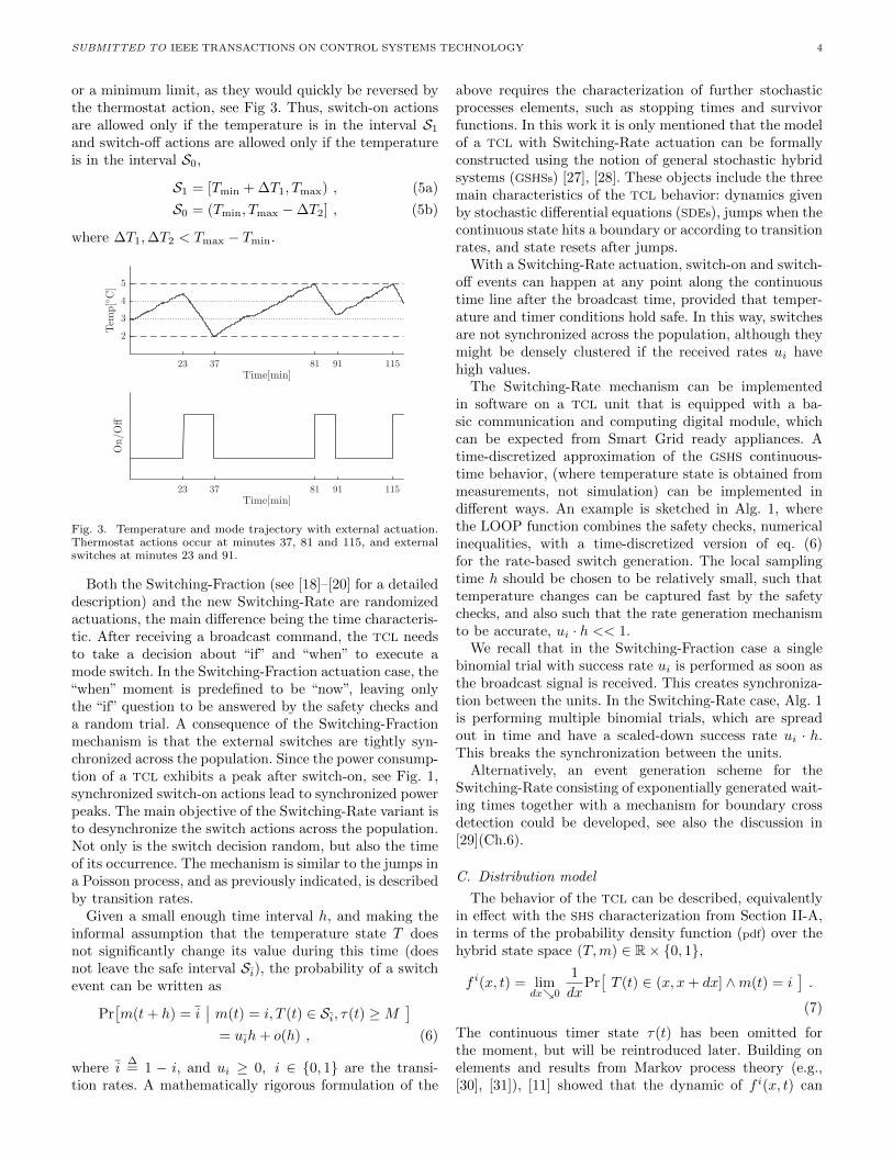
or a minimum limit, as they would quickly be reversed bythe thermostat action, see Fig 3. Thus, switch-on actionsare allowed only if the temperature is in the interval S1

and switch-off actions are allowed only if the temperatureis in the interval S0,

S1 = [Tmin + ∆T1, Tmax) , (5a)

S0 = (Tmin, Tmax −∆T2] , (5b)

where ∆T1,∆T2 < Tmax − Tmin.

Time[min]

On/Off

Time[min]

Tem

p[◦C]

23 37 81 91 115

23 37 81 91 115

2

3

4

5

Fig. 3. Temperature and mode trajectory with external actuation.Thermostat actions occur at minutes 37, 81 and 115, and externalswitches at minutes 23 and 91.

Both the Switching-Fraction (see [18]–[20] for a detaileddescription) and the new Switching-Rate are randomizedactuations, the main difference being the time characteris-tic. After receiving a broadcast command, the TCL needsto take a decision about “if” and “when” to execute amode switch. In the Switching-Fraction actuation case, the“when” moment is predefined to be “now”, leaving onlythe “if” question to be answered by the safety checks anda random trial. A consequence of the Switching-Fractionmechanism is that the external switches are tightly syn-chronized across the population. Since the power consump-tion of a TCL exhibits a peak after switch-on, see Fig. 1,synchronized switch-on actions lead to synchronized powerpeaks. The main objective of the Switching-Rate variant isto desynchronize the switch actions across the population.Not only is the switch decision random, but also the timeof its occurrence. The mechanism is similar to the jumps ina Poisson process, and as previously indicated, is describedby transition rates.

Given a small enough time interval h, and making theinformal assumption that the temperature state T doesnot significantly change its value during this time (doesnot leave the safe interval Si), the probability of a switchevent can be written as

Pr[m(t+ h) = i

∣∣ m(t) = i, T (t) ∈ Si, τ(t) ≥M]

= uih+ o(h) , (6)

where i∆= 1 − i, and ui ≥ 0, i ∈ {0, 1} are the transi-

tion rates. A mathematically rigorous formulation of the

above requires the characterization of further stochasticprocesses elements, such as stopping times and survivorfunctions. In this work it is only mentioned that the modelof a TCL with Switching-Rate actuation can be formallyconstructed using the notion of general stochastic hybridsystems (GSHSs) [27], [28]. These objects include the threemain characteristics of the TCL behavior: dynamics givenby stochastic differential equations (SDEs), jumps when thecontinuous state hits a boundary or according to transitionrates, and state resets after jumps.

With a Switching-Rate actuation, switch-on and switch-off events can happen at any point along the continuoustime line after the broadcast time, provided that temper-ature and timer conditions hold safe. In this way, switchesare not synchronized across the population, although theymight be densely clustered if the received rates ui havehigh values.

The Switching-Rate mechanism can be implementedin software on a TCL unit that is equipped with a ba-sic communication and computing digital module, whichcan be expected from Smart Grid ready appliances. Atime-discretized approximation of the GSHS continuous-time behavior, (where temperature state is obtained frommeasurements, not simulation) can be implemented indifferent ways. An example is sketched in Alg. 1, wherethe LOOP function combines the safety checks, numericalinequalities, with a time-discretized version of eq. (6)for the rate-based switch generation. The local samplingtime h should be chosen to be relatively small, such thattemperature changes can be captured fast by the safetychecks, and also such that the rate generation mechanismto be accurate, ui · h << 1.

We recall that in the Switching-Fraction case a singlebinomial trial with success rate ui is performed as soon asthe broadcast signal is received. This creates synchroniza-tion between the units. In the Switching-Rate case, Alg. 1is performing multiple binomial trials, which are spreadout in time and have a scaled-down success rate ui · h.This breaks the synchronization between the units.

Alternatively, an event generation scheme for theSwitching-Rate consisting of exponentially generated wait-ing times together with a mechanism for boundary crossdetection could be developed, see also the discussion in[29](Ch.6).

C. Distribution model

The behavior of the TCL can be described, equivalentlyin effect with the SHS characterization from Section II-A,in terms of the probability density function (pdf) over thehybrid state space (T,m) ∈ R× {0, 1},

f i(x, t) = limdx↘0

1

dxPr[T (t) ∈ (x, x+ dx] ∧m(t) = i

].

(7)

The continuous timer state τ(t) has been omitted forthe moment, but will be reintroduced later. Building onelements and results from Markov process theory (e.g.,[30], [31]), [11] showed that the dynamic of f i(x, t) can


Algorithm 1 Switching-Rate

global T,m, τ, u0, u1

const ∆T1,∆T2,M, h

function BroadcastReceived(new u0, new u1)u0 ← new u0 . ”←” denotes an assign operationu1 ← new u1

end function

function loop( ) . called 1/h-times per secondif (m == 1) and (T > Tmin) and (T ≤ Tmax −

∆T2) and (τ ≥M) and (rand() ≤ u0 · h) thenm← 0

end ifif (m == 0) and (T < Tmax) and (T ≥ Tmin +

∆T1) and (τ ≥M) and (rand() ≤ u1 · h) thenm← 1

end ifend function

be described analytically. In particular, the dynamic off i(x, t) represents the generator of the forward linearsemigroup associated with the SHS model of the TCL. Fordynamical systems characterized by regular SDEs, withouthybrid elements, this generator is known as the Fokker-Planck equation and can be seen as a transport andconservation law for probability. Therefore, the result in[11] is a type of Fokker-Planck operator specific to the TCL

SHS without actuation. The advantage of this modeling isthat, unlike the SHS form, a TCL description in terms ofthe pdf translates almost directly into a (homogeneous)population model. Probability quantities simply changemeaning to population fractions, see e.g., [11], [13], [14].

1) Distribution model without actuation: This sectionintroduces the main result from [11] that gives the dynam-ics of f i(x, t) in the form of a PDE system with boundaryconditions. Before stating the result, some preliminariesare addressed.

The temperature domain is divided into three sub-sets: the thermostat range Sb = [Tmin, Tmax], and Sa =(−∞, Tmin) and Sc = (Tmax,∞). This is a natural di-vision with respect to the operation of the TCL, and isnecessary because boundary conditions apply in the pointsTmin and Tmax, and because the pdf f i(x, t) is not x-differentiable here. Superscript indices will be used todenote subcomponents of the pdf functions f i(x, t) over thespecific partitions, e.g., f0a or f1b. Temperatures outsidethe thermostat range must be accounted for because ofthe diffusive component in the thermal dynamics (1). Forexample, even though the TCL is automatically “on” andstarting to cool when T (t) = Tmax, the temperature mightreach values T (t) > Tmax due to the contribution of thewhite noise (diffusive) term. It is also important to notethat the pdf corresponding to the off mode, f0(x, t), iszero-valued on the Sc domain, because if the temperaturebecomes greater than Tmax the thermostat mechanismensures that the mode can not remain “off”. Similarly, the

Tminmin Tmin Tmax Tmaxmax

f0a

f0b

f1c

∆T1 ∆T2

f0b1 f0b2

f1b1 f1b2 f1b3

f0b3

f1b

Fig. 4. Partitions of the temperature domain and subcomponents

pdf corresponding to the on-mode, f1(x, t) is zero-valuedon the Sa domain. In numerical work, the infinity domainslimits can be bounded since it is realistic to assume thatthe temperature inside a working refrigerator will notdrop below some Tminmin value and cannot rise abovesome Tmaxmax value, or equivalently, that probability ofthis happening is sufficiently low that it can be ignored.These elements are summarized on Fig. 4, using the pdf

equilibrium profile corresponding to the refrigerator unitfrom Section IV. Additionally, Fig. 4 contains notationsb1, b2 and b3 for the intervals (Tmin, Tmin + ∆T1), [Tmin +∆T1, Tmax−∆T2] and (Tmax−∆T2, Tmax), relevant for theactuation part. With this notation, the safe-temperaturezones (5) can be expressed as

S0 = Sb1 ∪ Sb2 ; S1 = Sb2 ∪ Sb3 . (8)

The evolution of the temperature state T (t) in the interiorof the Sj domains, j ∈ {a, b, c}, is driven only by the SDE

component (since the discrete dynamics only come intoplay at the boundaries of the Sj domains). As a result, thedynamic of the pdf f ij(x, t) on the interior Sj is given bystandard Fokker-Planck equations matching the thermaldynamics (1b) for the corresponding mode,

∂f0j(x, t)

∂t+

∂

∂x

((αx+ β)f0j(x, t)

)=σ2

2

∂2f0j(x, t)

∂x2,

j ∈ {a, b} (9a)

∂f1j(x, t)

∂t+

∂

∂x

((αx+ β + γ)f1j(x, t)

)=σ2

2

∂2f1j(x, t)

∂x2,

j ∈ {b, c}. (9b)

The switching dynamics (3) are included in the bound-ary conditions. We first introduce the probability flowshij(x, t) as the integral over the temperature (x-) coor-


dinate of the probability fluxes ∂fij

∂t (x, t),

h0j(x, t) = −(αx+ β)f0j(x, t) +σ2

2

∂f0j(x, t)

∂x, (10a)

h1j(x, t) = −(αx+ β + γ)f1j(x, t) +σ2

2

∂f1j(x, t)

∂x.

(10b)

The boundary conditions can then be written as

h0a(Tminmin, t) = 0, h1c(Tmaxmax, t) = 0, (11a)

f1b(Tmin, t) = 0, f0b(Tmax, t) = 0, (11b)

f0b(Tmin, t) = f0a(Tmin, t),

f1b(Tmax, t) = f1c(Tmax, t), (11c)

h0a(Tmin, t) = h0b(Tmin, t) + h1b(Tmin, t), (11d)

h1c(Tmax, t) = h0b(Tmax, t) + h1b(Tmax, t). (11e)

Equations (11a) represent impenetrable wall conditions,i.e. there is no probability flow out-of or in-to the domainSa from the left side, and similarly there is no flowout-of or in-to the domain Sc from the right side. Therest of the boundary conditions are associated with thethermostat switching mechanism. First, (11b) account forthe “absorption” action of the thermostat switch on thediffusion dynamic, causing Pr[ T (t) = Tmin∧m(i) = 1 ] = 0and Pr[ T (t) = Tmax ∧ m(i) = 0 ] = 0. Second, the factthat the temperature state does not jump (is not reset)by the switching mechanism is reflected in the continuitycondition (11c). Finally, (11d) and (11e) describe of theflow of probability from mode “on” to mode “off” at Tmin,and the flow of probability from mode “off” to mode “on”at Tmax.

The above boundary conditions reduce to the morefamiliar form presented in [11], [14] and others, if they aremade explicit by introducing the flow functions expressions(10), and carrying out the arithmetical simplifications. Theform presented here, using flow functions h, can also beused in the case when considering other forms for thecontinuous dynamics of the hybrid branches in (1), e.g.using different diffusion coefficients for each mode.2) Finite-volume methods: The system (9), together

with boundary conditions (11), represents a linear, infinite-dimensional dynamic. We approximate it with a finite-dimensional form using finite-volume methods (FVM) [32],[33]. While other works use a finite-difference approach[15], [34], FVM are arguably more suitable. A main argu-ment is that FVM preserve the invariant of the continuoussystem in the discretized solution, in this case probability(probability will always amount to 1 in the numericalsolution).

FVM consist of three main steps. First, the continuousspatial domain (in this case, the temperature domain) ispartitioned using a relatively fine grid of non-overlappingcells2. The second step consists of building the FVM

2This is the semi-discrete FVM approach, as only the spatialdomain is discretized. The result is a finite-dimensional, continuous-time dynamic in the form of an ordinary differential equation system.The discrete-time dynamics can be obtained later, and separate fromthe spatial discretization process. Fully-discrete FVM techniques gridthe spatial and temporal coordinate simultaneously.

equation. This is done by integrating the dynamical PDE

equation over a cell of the grid. For a generic conservationdynamic in one spatial dimension x with drift field φ(x, t),

diffusion coefficient D = σ2

2 , and source term s(x, t),

∂ρ

∂t(x, t) +

∂(φ(x, t)ρ(x, t)

)∂x

= D∂2ρ(x, t)

∂x2+ s(x, t), (12)

integrating over the spatial cell Kq gives∫Kq

∂ρ

∂t(x, t)dx =

(− φ(x, t)ρ(x, t) +D

∂ρ(x, t)

∂x

)∣∣∣∣K+q

K−q

+

∫Kq

s(x, t)dx , (13)

where q ∈ {1, . . . , N} is the cell index, and K−q ,K+q are

the left and right edge points of the cell. Notice that flowquantities evaluated at K−q appear with a negative sign(outgoing) in the dynamic of the cell Kq, and with apositive sign (incoming) in the dynamic of the cell Kq−1.The outgoing flow from one cell is incoming flow to theneighbor cell, resulting in the conservative property ofthe method (in this way, the system invariant will notchange/be corrupted by the numerical steps). Next, theleft side of (13) can be further expressed as∫

Kq

∂ρ

∂t(x, t)dx =

d

dt

∫Kq

ρ(x, t)dx = ∆xqdΘq

dt(14)

with Θq the average value of ρ(x, t) over the cell Kq and∆xq the cell size. Equations (13) and (14) can be combinedto give the exact expression for the evolution in time of theaverage quantity Θq,

∆xqdΘq

dt=

(− φ(x, t)ρ(y, t) +D

∂ρ(x, t)

∂x

)∣∣∣∣K+q

K−q

+

∫Kq

s(x, t)dx . (15)

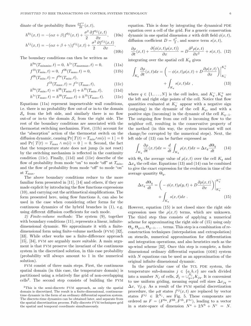
However, equation (15) is not closed since the right sideexpression uses the ρ(x, t) terms, which are unknown.The third step thus consists of applying a numericalscheme for approximating the right side of (15) using onlyΘq,Θq+1,Θq−1, . . . terms. This step is a combination of re-construction techniques (interpolation and extrapolation)on stencils, numerical approximation for differentiationand integration operations, and also heuristics such as theup-wind scheme [32]. Once this step is complete, a finitedimensional ordinary differential equation (ODE) systemwith N equations can be used as an approximation of theoriginal infinite dimensional dynamic.

In the particular case of the TCL PDE system, thetemperature sub-domains j ∈ {a, b, c} are each divided

into a number Nj of cells, Sj = ∪Nj

q=1Kjq. It is convenientto use uniform griding, meaning equal cell sizes ∆xjq =∆x, ∀j, q. As a result of the FVM spatial discretizationprocedure, the pdf states f ij(x, t) are replaced by vectorstates F ij ∈ RNj , see Fig. 5. These components areordered as F = (F 0a, F 0b, F 1b, F 1c), leading to a vectorin a state-space of dimension Na + 2N b + N c = N .


Tminmin Tmin Tmax Tmaxmax

F 0a

F 0b

F 1c

∆T1 ∆T2

F 0b1 F 0b2

F 1b1 F 1b2 F 1b3

F 0b3

F 1b∆x

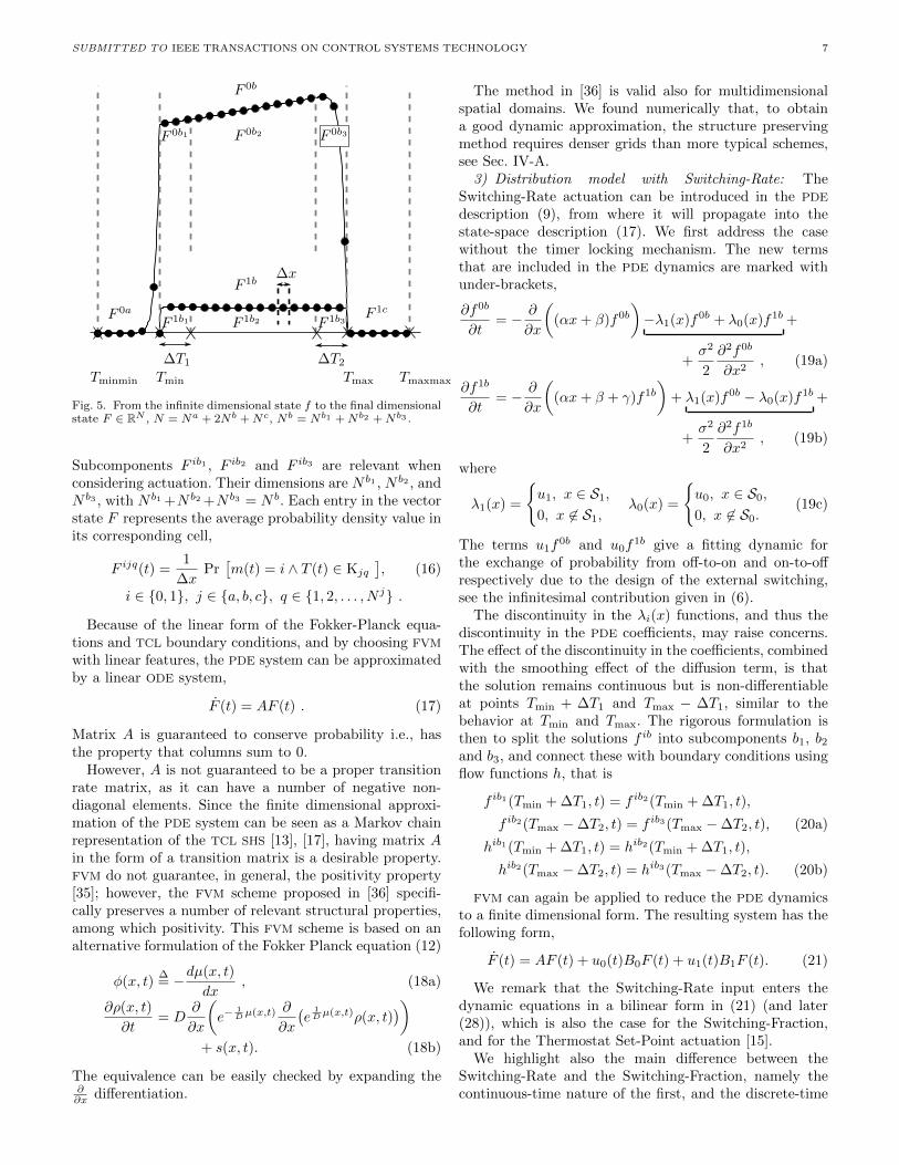
Fig. 5. From the infinite dimensional state f to the final dimensionalstate F ∈ RN , N = Na + 2Nb +Nc, Nb = Nb1 +Nb2 +Nb3 .

Subcomponents F ib1 , F ib2 and F ib3 are relevant whenconsidering actuation. Their dimensions are N b1 , N b2 , andN b3 , with N b1 +N b2 +N b3 = N b. Each entry in the vectorstate F represents the average probability density value inits corresponding cell,

F ijq(t) =1

∆xPr[m(t) = i ∧ T (t) ∈ Kjq

], (16)

i ∈ {0, 1}, j ∈ {a, b, c}, q ∈ {1, 2, . . . , N j} .

Because of the linear form of the Fokker-Planck equa-tions and TCL boundary conditions, and by choosing FVM

with linear features, the PDE system can be approximatedby a linear ODE system,

F (t) = AF (t) . (17)

Matrix A is guaranteed to conserve probability i.e., hasthe property that columns sum to 0.

However, A is not guaranteed to be a proper transitionrate matrix, as it can have a number of negative non-diagonal elements. Since the finite dimensional approxi-mation of the PDE system can be seen as a Markov chainrepresentation of the TCL SHS [13], [17], having matrix Ain the form of a transition matrix is a desirable property.FVM do not guarantee, in general, the positivity property[35]; however, the FVM scheme proposed in [36] specifi-cally preserves a number of relevant structural properties,among which positivity. This FVM scheme is based on analternative formulation of the Fokker Planck equation (12)

φ(x, t)∆= −dµ(x, t)

dx, (18a)

∂ρ(x, t)

∂t= D

∂

∂x

(e−

1Dµ(x,t) ∂

∂x

(e

1Dµ(x,t)ρ(x, t)

))+ s(x, t). (18b)

The equivalence can be easily checked by expanding the∂∂x differentiation.

The method in [36] is valid also for multidimensionalspatial domains. We found numerically that, to obtaina good dynamic approximation, the structure preservingmethod requires denser grids than more typical schemes,see Sec. IV-A.

3) Distribution model with Switching-Rate: TheSwitching-Rate actuation can be introduced in the PDE

description (9), from where it will propagate into thestate-space description (17). We first address the casewithout the timer locking mechanism. The new termsthat are included in the PDE dynamics are marked withunder-brackets,

∂f0b

∂t= − ∂

∂x

((αx+ β)f0b

)−λ1(x)f0b + λ0(x)f1b +

+σ2

2

∂2f0b

∂x2, (19a)

∂f1b

∂t= − ∂

∂x

((αx+ β + γ)f1b

)+ λ1(x)f0b − λ0(x)f1b +

+σ2

2

∂2f1b

∂x2, (19b)

where

λ1(x) =

{u1, x ∈ S1,

0, x 6∈ S1,λ0(x) =

{u0, x ∈ S0,

0, x 6∈ S0.(19c)

The terms u1f0b and u0f

1b give a fitting dynamic forthe exchange of probability from off-to-on and on-to-offrespectively due to the design of the external switching,see the infinitesimal contribution given in (6).

The discontinuity in the λi(x) functions, and thus thediscontinuity in the PDE coefficients, may raise concerns.The effect of the discontinuity in the coefficients, combinedwith the smoothing effect of the diffusion term, is thatthe solution remains continuous but is non-differentiableat points Tmin + ∆T1 and Tmax − ∆T1, similar to thebehavior at Tmin and Tmax. The rigorous formulation isthen to split the solutions f ib into subcomponents b1, b2and b3, and connect these with boundary conditions usingflow functions h, that is

f ib1(Tmin + ∆T1, t) = f ib2(Tmin + ∆T1, t),

f ib2(Tmax −∆T2, t) = f ib3(Tmax −∆T2, t), (20a)

hib1(Tmin + ∆T1, t) = hib2(Tmin + ∆T1, t),

hib2(Tmax −∆T2, t) = hib3(Tmax −∆T2, t). (20b)

FVM can again be applied to reduce the PDE dynamicsto a finite dimensional form. The resulting system has thefollowing form,

F (t) = AF (t) + u0(t)B0F (t) + u1(t)B1F (t). (21)

We remark that the Switching-Rate input enters thedynamic equations in a bilinear form in (21) (and later(28)), which is also the case for the Switching-Fraction,and for the Thermostat Set-Point actuation [15].

We highlight also the main difference between theSwitching-Rate and the Switching-Fraction, namely thecontinuous-time nature of the first, and the discrete-time


nature of the second. For piecewise-constant input signals,discrete-time form of (21), is

F (k + 1) = e

(A+u0(k)B0+u1(k)B1

)∆tF (k), (22)

which is not equivalent to the Switching-Fraction model,

F (k + 1) =(eA∆t + u0(k)B0 + u1(k)B1

)F (k) . (23)

4) Timer-Lock modeling: The modeling principle for thetimer-lock is to explicitly track the part of the pdf that be-comes locked for the external actuation. Two density func-tions are introduced to correspond to the locked conditionfor mode “off” and for mode “on”, L0 : (Tminmin, Tmax) ×[0,M)× [0,∞)→ R+ and L1 : (Tmin, Tmaxmax)× [0,M)×[0,∞)→ R+,

Li(x, y, t) = limdx↘0

dy↘0

1

dxdyPr[T (t) ∈ (x, x+ dx] ∧

∧ τ(t) ∈ (y, y + dy] ∧m(t) = i]. (24)

The part of f i(x, t) which remains responsive to theactuation is evaluated by subtracting the probability ofbeing locked, and the following updates are made to (19a)and (19b),

λ1(x)f0b → λ1(x)

f0b −

amount of locked f0b∫ M

0

L0(x, y, t)dy

, (25a)

λ0(x)f1b → λ0(x)

f1b −

amount of locked f1b∫ M

0

L1(x, y, t)dy

. (25b)

The dynamics of Li are given by standard Fokker-Planckequations in the two-dimensional state space (T, τ) (tem-perature and timer state), with the underlying processdriven by (1b) and (4), with no external switching con-tributions. The dynamics are thus,

∂Li

∂t(x, y, t) = − ∂

∂x

((αx+ β + iγ)Li(x, y, t)

)−

− ∂

∂yLi(x, y, t) +

σ2

2

∂2

∂x2Li(x, y, t) , (26)

with boundary conditions,

hL0(Tminmin, y, t) = 0, hL1(Tmaxmax, y, t) = 0, (27a)

L1(Tmin, y, t) = 0, L0(Tmax, y, t) = 0, (27b)

Li(x, 0, t) = λi(x, t)(f ib(x, t)−

∫ M

0

Li(x, y, t)dy). (27c)

Equations (27a) represent impenetrable walls conditionswhere the probability flow h defined in (10) is zero, and(27b) represent absorbing boundaries due to the ther-mostat action. Finally, (27c) accounts for the incomingprobability of a new switching event and the zero reset ofthe timer state. This is a condition that has discontinuitiesin the x-space and in time, see (19c) and the fact that

ui(t) is, due to the nature of broadcast communication,a piecewise constant function. Again, discontinuities canbe a problem for the current mathematical description.A solution can be to modify the TCL behavior to anideal version where a smooth approximate of the λi(x, t)is used. However, such modifications do not change anyof the practical considerations and have little impact onthe results of the computational algorithms, includingthe FVM procedure. The main difference introduced bythe modeling of the locking mechanism is that a twodimensional FVM scheme needs to be used for the stateLi. The final form of the finite-dimensional dynamic is,

X(t) = AXX(t) + u0(t)BX0 X(t) + u1(t)BX1 X(t) ,

X = (F, L0, L1) , (28)

where L0 ∈ R(Na+Nb)Md , L1 ∈ R(Nb+Nc)Md , X ∈RN(Md+1), and Md is the number of grid cells with size ∆yused to discretize the timer-state domain [0,M ]. A linearcoordinate change can be used to create a Markov chainformulation, by separating the unlocked from the lockedstates,

X ′ =(F 0 −∆y

Md∑l=1

off, locked, τ∈[(l−1)∆y,l∆y)

L0(l−1)Na+b+1:lNa+b

,

F 1 −∆y

Md∑l=1

on, locked, τ∈[(l−1)∆y,l∆y)

L1(l−1)Nb+c+1:lNb+c

,

L0, L1)

= TXX , (29)

where TX denote the coordinate change defined by the left-hand side of (29) and X ′ denote X in the new coordinates.

Locking effects after a thermostatic switch are not con-sidered. The reason why this is not necessary is due tothe temperature safe-zones feature. After a thermostaticswitch, the unit is prevented from switching again until itis some distance ∆T away from the thermostat boundary.This temperature distance can be chosen such that itseffects are practically equivalent to a timer condition.

This completes the main part of the Switching-Ratemodeling.

5) Model output and extension: The expected powerconsumption output of a TCL can be obtained by calculat-ing the total probability of a unit being “on”, and scalingit with the power rating parameter W ,

z(t) = CF (t), (30)

with C = W∆x[01×(Na+Nb) 11×(Nb+Nc)

].

The Fokker-Planck approach to modeling the distribu-tion dynamics can also be used when considering otherelements in the TCL model, such as nonlinear terms orjump noises. Another remark is that coefficients and pa-rameters characterizing the dynamical behaviors can takedifferent values in mode “on” compared to mode “off”, forexample the entire drift field, the diffusion coefficients, andtemperature safe zones ∆T , and the timer setting M .


6) Population Heterogeneity: As mentioned, when con-sidering a large group of units with identical parameters(a homogeneous population), probabilities simply changemeaning to fractions. This means that models (21) and(28) can be initialized in with values for F (or X) re-flecting the fraction distribution of the temperature andmode (and timer) values across the population, instead ofthe probability distribution of a unit’s initial state. Thedynamics with naturally propagate the distributions overtime and under inputs.

Small heterogeneities of the TCL population should notcause severe modeling errors, but large heterogeneities willcause a significant departure from the homogeneous case.However, exact modeling of heterogeneous population isimpractical since it suffers from “curse of dimensionality”(the distribution state-space needs to be extended with anextra dimension for each parameter). Therefore, hetero-geneity is not explicitly accounted for in the distributionmodel. Instead, this work makes use of the fact that theswitching actuation has a certain amount of robustness tomodel variations due to its percentage formulation, andfurthermore, measurements and estimations can be usedto periodically update the distribution state in real-timeoperation.

For a more pronounced dispersion of parameters, aclustering strategy e.g., [18], should be applied first. There-fore, the models and control proposed in this work are tobe applied for each individual cluster in a heterogeneouspopulation. In the numerical simulations, moderate levelsof heterogeneity are considered for the TCL population.

III. Model-based Control Algorithms

This section presents two model-based control al-gorithms that can be used to manipulate the aggre-gated power consumption of the TCL population via theSwitching-Rate actuation. The control objective is to havethe power output track an input reference. At the end,considerations are made about the measurement channels.

A. Control System

The TCL population model has a continuous-time, bilin-ear [37], [38], homogeneous input form, for both the basicand timer-lock augmented versions,

F (t) =(A+

∑i

ui(t)Bi)F (t), (31a)

X(t) =(AX +

∑i

ui(t)BXi

)X(t) , (31b)

with ui ∈ [0, umax]. The aggregated power consumption isa linear combination of the states,

za(t) = nCF (t), (32)

where n is the number of units in the population, and forthe timer-lock augmented system F is recovered as thefirst N -coordinates in X according to (28).

The free dynamics of the system are given by matrixA, which has stable eigen values, except one which is

exactly zero. This is due to the FVM procedure producinga dynamic matrix that conserves the probability invariantof the system state, by having columns that sum to 0. Thisfact can be used to reduce the system dimension by onestate. Given an initial state F (0) such that the sum ofits elements is f (in particular f = 1

∆x ), the sum of theF (t) elements will remain equal to f . Therefore, one of thestates can be written as the difference between f and thesum of all others.

F (t) =

[F (t)FN (t)

], F ∈ RN−1, FN ∈ R, (33a)[

˙F

FN

]=

([A11 A12

A21 a22

]+∑i

ui

[Bi,11 Bi,12

Bi,21 bi,22

])[FFN

],

(33b)

FN = f − 1TN−1F , (33c)

˙F = A11F +A12(f − 1TN−1F ) +∑i

uiBi,11F ,

=

(A+

∑i

uiBi

)F + a. (33d)

In (33b) matrix Bi,12 = 0 for the switching actuation(because FN belongs to the c-temperature domain, whichis not affected by the actuation), in (33d) A = A11 −A121TN−1 ∈ R(N−1)×(N−1), a = A12f and Bi = Bi,11 . Thedynamical system matrix A of the transformed system isHurwitz. Furthermore, a change of variables can move theequilibrium state of the affine system (33d) to 0, resultingin linear, stable free dynamic at the expense of an addedaffine input term,

F0 = F + A−1a , (34a)

˙F0 =

(A+

∑i

uiBi

)F0 −

∑i

ui

bi

BiA−1a . (34b)

In summary, we started with matrix A which has a one-dimensional null-space, identified the equilibrium state inthe null-space by the ”sums to f” constraint given bythe initial state, and then shifted the equilibrium to zerousing a change of variable. Notice also that the equilibriumdistribution can be calculated as

Fe =[−A−1a, f + 1TN−1

(A−1a

)]. (35)

The same process of changing from a marginally stable toa fully stable dynamic description can be applied to theAX timer-lock system matrix. Since the algorithms usedin this work do not require strict stability, in the followingwe will continue to use the forms (31).

B. Input Reference Tracking

This section presents two control algorithms for track-ing an external power reference. By necessity (the geo-graphically distributed nature of the control structure),all control algorithms operate in discrete-time. Thus, theTCLs maintain the switching rates u constant until thenext broadcast event (piecewise constant actuation). The


first algorithm uses switch-off and switch-on actions oneat a time, while the second algorithm uses an energystorage heuristic and simultaneous switch-off and switch-on actions. The algorithms use the distribution modelas internal model, and measurements of the total powerconsumption at every step, perform calculations or opti-mizations over short time horizons, and require an esti-mate for the initial state (which is expected to be close toequilibrium in the absence of actuation). The algorithmscan benefit from - but do not require - frequently updatedstate information. The control structure is shown in Fig. 6.

Σ

z1

z2

zn

z3

........................

ST1 TCL1

ST2 TCL2

ST3 TCL3

STn TCLn

uController

za

FObserver

r

TCL population

Ti,mi, τi

Fig. 6. Controller structure. The dotted lines indicate signals withlow update frequency.

1) Basic reference tracking: The main elements of thefirst control strategy are sketched in Alg. 2. This is apredictive scheme with a single time-step lookahead. First,a prediction is made about the power output in the absenceof control. If this is bigger than the reference r, the switch-off action is selected for activation. In the opposite case,the switch-on action is selected. Consequently, the mainstep consists of calculating the precise input value thatwould bring the internal model of the controller to thedesired reference. An input-output linearization technique[39] is used, together with the simplified assumption thatthe output velocity remains constant in the control sampletime ∆t,

za(k + 1) = za(k) + za(k)∆t , (36a)

za(k) = nCAF (k) + ui(k)nCBiF (k) , (36b)

ui(k) =−nCAF (k) + v

nCBiF (k), (36c)

za(k + 1) = za(k) + v∆t , (36d)

v =r(k + 1)− za(k)

∆t, (36e)

where (36d) is obtained from (36a)-(36c). For robustnessto heterogeneity and other prediction errors, the actuationis wrapped in an error integration structure (PI control),preferably with anti-windup. Algorithm 2 is suitable forboth the simple and the augmented models, since thecomputation load is light. In Alg. 2, the integration gainKi is a design parameter.

While arguably practical, Alg. 2 manages the powerflexibility of the TCL population in a simplistic manner.

Algorithm 2 Step k

e = Kie+ za(k)− r(k) . tracking error at kep = nCeA∆tF (k)− (r(k + 1)− e)

. predicted error at k + 1 if no actuation is usedif ep > 0 then . Need to decrease output, use u0

u0(k) = Control(B0)else if ep < 0 then . Need to increase output, use u1

u1(k) = Control(B1)end if

function control(B)v =

(r(k + 1)− za(k)

)/∆t

u =(− nCAF (k) + v

)/(nCBF (k)

)u =Limit(u,0,umax) . saturation cutF (k + 1) = e(A+uB)∆tF (k)return u

end function

This is because, in most cases, there exists more than oneactuation option for bringing the output of the system tothe reference power consumption r(k + 1). By having alookahead horizon of just one step, and using a presetstrategy for choosing between the actuation options, Alg. 2is not able to track challenging references. An example ofa challenging reference is a step-down to zero.

2) Zero power reference: The second control algorithmis an example of heuristics that can maintain a zero power-reference over a time horizon of reasonable length. Thiscontrol uses a slightly modified version of the switching ac-tion. Since the TCL temperature sensor is already requiredto distinguish between three domains in the thermostatband (b1,b2,b3), we can consider an actuation variant withfour input channels: u0b1 , u0b2 , u1b2 and u1b3 . This meansthat it is possible to use one switch-off rate for the on-unitsin the temperature range Sb1 and another for the on-unitsin the temperature range Sb2 , and similarly, two differentswitch-on rates for the off-units in the Sb2 and Sb3 ranges.

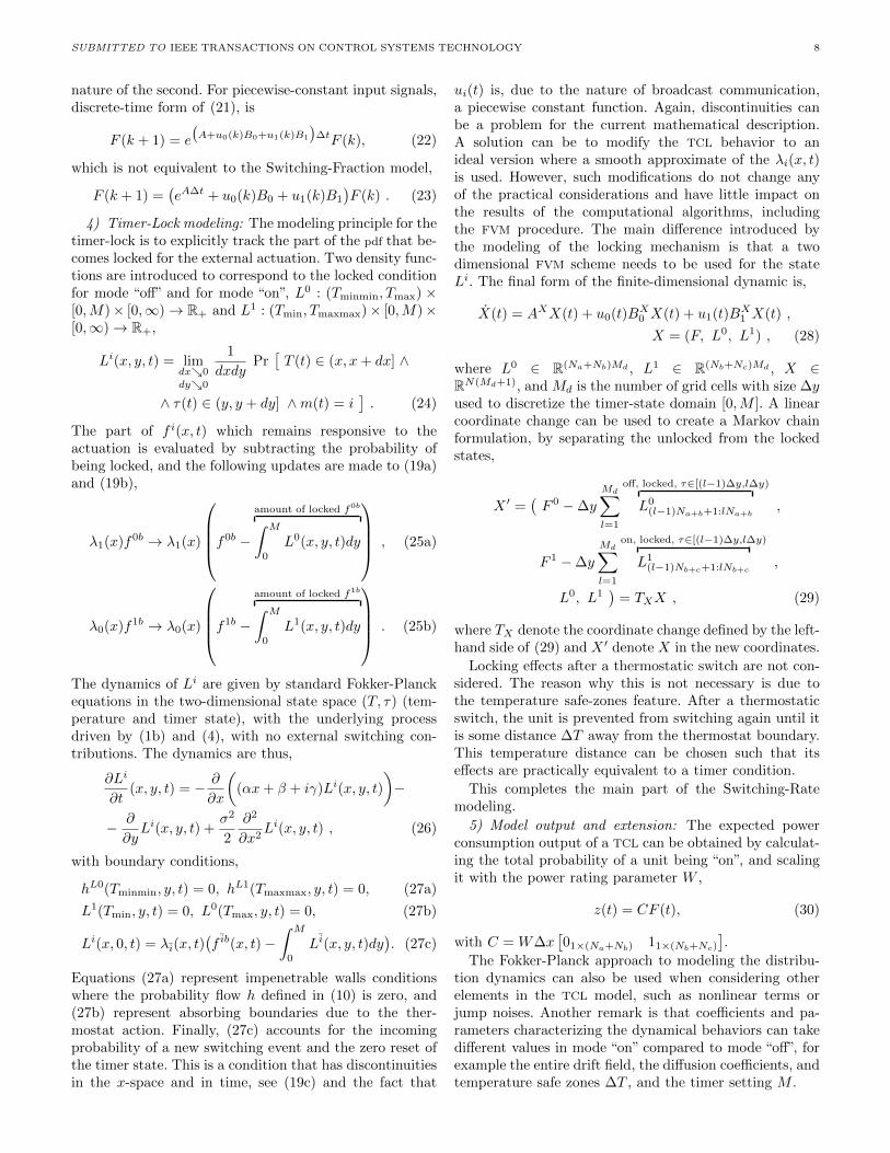
The control strategy is composed of three phases,sketched in Fig. 7. Each phase of the strategy is controlledby a different algorithm. In the first phase, the units arepushed away from the right (hot) thermostat band usingthe switch-on action u1b3. In order to keep the powerconsumption close to a normal level, this action must becompensated by switching-off units from the left (cold)side of the thermostat using the u0b1. The combined effectis equivalent to a narrowing of the thermostat band to theSb2 interval. In this operation mode, the duty cycle of aunit will be only slightly higher than the normal value, andthe aggregated power output of the population can remainclose to the baseline value. The second phase correspondsto the zero power consumption period. The on- and off-distributions are now collected in the midband range Sb2 .Therefore, it is possible to switch-off all units using inputu0b2 . Power consumption will remain zero as the collectedoff-distribution is slowly moving right (heating) acrossthe Sb1 domain and up until the Tmax threshold of the


thermostat is reached. The third stage is recovery. Thepopulation needs to be controlled so as to slowly return tothe equilibrium distribution, while maintaining a powerconsumption level close to the baseline. We do not solvethe recovery problem in this work, but simply apply Alg. 2to return power consumption to the baseline level. Wenotice that in this way the system output is returned andmaintained to the equilibrium values, but not also thesystem state.

Algorithm 3 details this second control strategy. Thestorage phase consists of a multi-objective optimizationover each control sample time,

minimizeu1b3

(k),u0b1(k)

[ − u1b3 ,P∑p=1

(nCX(p)− r(p))2]

subject to

X(0) = F (k) ,X(p+ 1) = exp

((A+

∑j∈{1b3,0b1}

uj(k)BjX(p))

∆tP

)X(p) ,

u1b3(k) ≥ 0 ,u0b1(k) ≥ 0 .

We want to switch-on as many units as possible usingu1b3, and compensate by the switching-off action u0b1 inorder to keep the power consumption close to a baselinereference. To avoid large fluctuations within the con-trol sample time ∆t, the reference tracking objective isformulated using a series of p intra-period time points.The multi-objective optimization was implemented usingfgoalattain() MATLAB R© function, based on the goalattainment method [40]. While the optimization approachhas the potential of becoming computationally heavy, itis sufficient to use the unaugmented distribution modelfor both populations with and without minimum on/offtime constraints. This is because the input actions arewell separated between different temperature zones, thusalso separated in time, and the locking effect is inherentlyrespected. With this observation, Alg. 3 remains compu-tationally feasible.

C. Measurements

The main measurement used by the control algorithmis the total power consumption signal. This is the drivingsignal of the control loop structure. In this work, theTCL population has been considered in isolation, but in arealistic scenario aggregate power measurements from theelectrical grid will include other consumption. Therefore,a method would be needed to separate the contributionof the TCLs from the total consumption data. However,the control objective is not the TCL consumption per se,but rather the total consumption in an area (or portfolio).As long as the control objective can be measured, it canbe used directly (without separation) to create the controlerror signal.

Monitoring the distribution state of a TCL populationover time requires individual unit measurements. Theadvantage of the distribution approach is that individualstate measurements can be infrequent, partial and are used

Algorithm 3 Step k

if phase(k+1) == “Storage” thene = Kie+ za(k)− r(k) . tracking error at k[ u0b1(k), u1b3(k)] = Optim(r(k + 1)− e)

else if phase(k+1) == “Discharge” thenu0b1(k) = umax, u0b2(k) = umax

else if phase(k+1) == “Recovery” thenuse Algorithm 2 . Partial recovery

end if

function Optim(r)p = 5 . no. of intra-period pointsir = linspace(za(k),r,p+ 1)

. intra-period reference profilelb = [0,0], ub =[umax, umax] . lower/upper boundsu = min-multi-objective(@objectives, lb, ub )return u

end functionfunction objectives(u)

Adn = e(A+u(1)B0b1+u(2)B1b3)(∆t/p)

Fp = F (k), obj(1) = 0for j = 1 to p do

Fp = AdnFpobj(1) = obj(1) +

(CFp − ir(j)

)2end forobj(2) = −u(2) . or equiv. −u(1)return obj

end function

anonymously. Individual unit measurements consists of thetemperature and mode (and timer) data from a limitednumber of units in the population, e.g., 10% or 20%. Thesecan be processed to create a distribution measurementF . The error of such a distribution measurement can becharacterized using the variance and covariance propertiesof the multivariate hypergeometric distribution. This isbecause by extracting a finite number of units nm from

Control

Discharge

Storage

Recover

Fig. 7. The stages of the second control algorithm.


the TCL population with n > nm units and N possibleoutcomes, we are effectively performing a “draws withoutreplacement” random experiment. Furthermore, the dy-namical models (31), could be equipped with error models,see the approach in [13]. We do not, however, address thecomplete estimation problem in this work.

IV. Numerical simulations

This section contains numerical results on a case-studyfor domestic refrigerators. The equivalent thermal param-eters used for the TCL model (1a) are listed in Table I.The actuation parameters are the minimum on/off timeM = 300s, the temperature safe-zones are ∆T1 = ∆T2 =1◦C, and umax = 2.

TABLE IParameters of the TCL

C (J/K) UA (W/K) Ta (◦C ) W (W)93920 1.432 24 100η σ (◦C/s) Tmin(◦C) Tmax(◦C)2.8 0.0065 2 5

In all cases, a population of 10000 units is considered.In addition to the homogeneous population, two typesof heterogeneities, each with three increasing levels, havebeen tested. The parameters have been randomly dis-tributed around the mean values from Table I accordingto a 3σ-truncated Gaussian distribution with standard de-viations of 5%, 10%, and 15%, and according to a uniformdistribution with standard deviations of 10%, 20%, and30%. The C, UA, Ta, η, W , and σ parameters have beenaffected, while the thermostat range, temperature safe-zones and the minimum on/off time are the same acrossthe population. The TCL population has been simulatedusing Monte Carlo techniques. Each of the 10000 SHSmodels is run individually with a sample rate of 0.1s. Forcontrol, a broadcast rate ∆t = 60s has been used.

A. FVM results

We first give a qualitative and quantitative comparisonfor the dynamical system matrix A obtained with differ-ent FVM implementation. In all cases, the FVM grid isuniform, with domain boundaries Tminmin = 1.5◦C andTmaxmax = 5.5◦C. Four cases are compared: a second orderup-wind scheme with a coarse (a) and dense (b) grid, andthe structure preserving FVM (see end of Sec. II-C2) on acoarse (c) and on a dense (d) grid.

TABLE IIDynamic matrix A

∆x N Positivity Duty Cycle(a) 0.0385 182 No 0.105(b) 0.01 700 No 0.105(c) 0.0385 182 Yes 0.04878(d) 0.0025 2800 Yes 0.1046

The duty cycle calculation is done using the equilib-rium distribution computed by (35) and evaluating the

percentage of represented by the total area under the on-distribution. It is used as an indicator for the absoluteerror of the FVM schemes. The duty cycle for a TCL withparameters from Table I is close to 0.105 value. Fig. 8shows the equilibrium distributions obtained from thefour methods. It can be seen that the second order up-wind scheme (a) is not positive, and shows the spuriousoscillation effects (see Godunov’s order barrier theorem,[33] ch.13), but both these effects are reduced when thegrid size is reduced in scheme (b). The structure preservingschemes (c) and (d) are positive, but slower to converge,and as a result the distribution (and duty cycle) of coarsescheme (c) has significant errors. Although accuracy cri-teria would suggest using schemes (d) or (b), scheme (a)has the advantage of a small computational footprint, andproves to capture the dynamical behavior suitably well forcontrol algorithms.

2 3 4 5−0.05

0.15

0.35

(a)

2 3 4 50

0.2

(b)

2 3 4 50

0.2

(c)

2 3 4 50

0.2

(d)

Fig. 8. Equilibrium distributions as obtained using the secondorder up-wind coarse and dense schemes (a) and (b) respectively,and the structure preserving coarse and dense schemes (c) and (d)respectively. The grid parameters are given in Table II.

Augmented systems have a higher dimensionality. Thespatial discretization and overall matrix size used in thefollowing control simulations is given in Table III.

TABLE IIIAugmented dynamic matrix AX

∆x ∆y N

AX 0.0385 30s 2002

B. Free response simulations

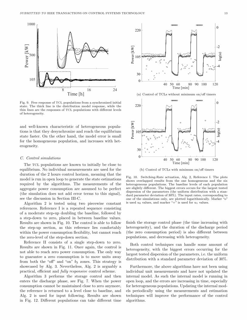
Figure 9 shows the free response from an initial statewhere all units are initially off and have the same tempera-ture, its value close to the hot threshold of the thermostat.

This synchronized initial state showcases the oscillatorynature of the power response, and the differences betweenthe homogeneous and heterogeneous populations. A main


Time [h]

Pow

er [

kW]

8 16 24

105

500

1000

Fig. 9. Free response of TCL populations from a synchronized initialstate. The thick line is the distribution model response, while thethin lines are the responses of TCL populations with different levelsof heterogeneity.

and well-known characteristic of heterogeneous popula-tions is that they desynchronize and reach the equilibriumstate faster. On the other hand, the model error is smallfor the homogeneous population, and increases with het-erogeneity.

C. Control simulations

The TCL populations are known to initially be close toequilibrium. No individual measurements are used for theduration of the 2 hours control horizon, meaning that themodel is run in open loop to generate the state estimationsrequired by the algorithms. The measurements of theaggregate power consumption are assumed to be perfect(the simulation does not add error terms to this signal),see the discussion in Section III-C.

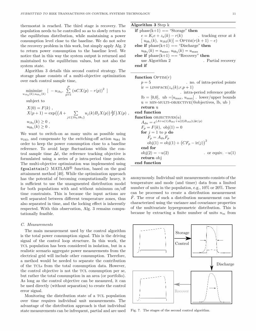
Algorithm 2 is tested using two piecewise constantreferences. Reference I is a repeated sequence consistingof a moderate step-up doubling the baseline, followed bya step-down to zero, placed in between baseline values.Results are shown in Fig. 10. The control is able to followthe step-up section, as this reference lies comfortablywithin the power consumption flexibility, but cannot reachthe zero-level of the step-down section.

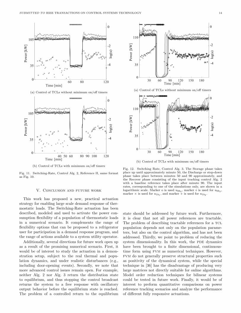
Reference II consists of a single step-down to zero.Results are shown in Fig. 11. Once again, the control isnot able to reach zero power consumption. The only wayto guarantee a zero consumption is to move units awayfrom both the “off” and “on” b3 zones. This strategy isshowcased by Alg. 3. Nevertheless, Alg. 2 is arguably apractical, efficient and fully responsive control scheme.

Algorithm 3 performs the storage control and thenenters the discharge phase, see Fig. 7. When the powerconsumption cannot be maintained close to zero anymore,the reference is returned to a level close to baseline, andAlg. 2 is used for input following. Results are shownin Fig. 12. Different populations can take different time

0

30

105

220

Pow

er [k

W]

log(

u)

Time [min]40 50 60 80 90 100 120

-4

-2

0

(a) Control of TCLs without minimum on/off timers

0

30

105

220

Pow

er [k

W]

log(

u)

Time [min]40 50 60 80 90 100 120

-4

-2

0

(b) Control of TCLs with minimum on/off timers

Fig. 10. Switching-Rate actuation, Alg. 2, Reference I. The plotsshows overlapped results from the one homogeneous and the sixheterogeneous populations. The baseline levels of each populationare slightly different. The biggest errors occurs for the largest testeddispersion of the parameters (the uniform distribution with a stan-dard parameter deviation of 30%). The input rates, corresponding toone of the simulations only, are plotted logarithmically. Marker “o”is used u0 values, and marker “+” is used for u1 values.

finish the storage control phase (the time increasing withheterogeneity), and the duration of the discharge period(the zero consumption period) is also different betweenpopulations, and decreasing with heterogeneity.

Both control techniques can handle some amount ofheterogeneity, with the biggest errors occurring for thelargest tested dispersion of the parameters, i.e. the uniformdistribution with a standard parameter deviation of 30%.

Furthermore, the above algorithms have not been usingindividual unit measurements and have not updated theinternal model. As such the internal model is running inopen loop, and the errors are increasing in time, especiallyfor heterogeneous populations. Updating the internal mod-els periodically using the measurements and estimationtechniques will improve the performance of the controlalgorithms.


0

35

105

Pow

er [k

W]

log(

u)

Time [min]60 80 120

-4

-2

0


0

35

105

Pow

er [k

W]

log(

u)

40 50 60Time [min]

80 90 100 120

-4

-2

0


Fig. 11. Switching-Rate, Control Alg. 2, Reference II, same formatas Fig. 10.

V. Conclusion and future work

This work has proposed a new, practical actuationstrategy for enabling large scale demand response of ther-mostatic loads. The Switching-Rate actuation has beendescribed, modeled and used to activate the power con-sumption flexibility of a population of thermostatic loadsin a numerical scenario. It complements the range offlexibility options that can be proposed to a refrigeratoruser for participation in a demand response program, andthe range of actions available to a system utility operator.

Additionally, several directions for future work open upas a result of the promising numerical scenario. First, itwould be of interest to study the actuation in a demon-stration setup, subject to the real thermal and popu-lation dynamics, and under realistic disturbances (e.g.,including door-opening events). Secondly, we note thatmore advanced control issues remain open. For example,neither Alg. 2 nor Alg. 3 return the distribution stateto equilibrium, and thus stopping the control broadcastreturns the system to a free response with oscillatoryoutput behavior before the equilibrium state is reached.The problem of a controlled return to the equilibrium

0

35

110

Pow

er [

kW]

log(

u)

Time [min]30 60 90 120 150 180

-4

-2

0


0

35

110

Pow

er [k

W]

log(

u)

Time [min]30 60 90 120 150 180

-4

-2

0


Fig. 12. Switching Rate, Control Alg. 3. The Storage phase takesplace up until approximately minute 50, the Discharge or step-downphase takes place between minutes 50 and 90 approximately, andthe Recover phase consisting of the input tracking control Alg. 2with a baseline reference takes place after minute 90. The inputrates, corresponding to one of the simulations only, are shown in alogarithmic scale. Marker o is used u0b2 , marker � is used for u0b3 ,marker × is used for u1b1 , and marker + is used for u1b2 .

state should be addressed by future work. Furthermore,it is clear that not all power references are tractable.The problem of describing tractable references for a TCL

population depends not only on the population parame-ters, but also on the control algorithm, and has not beenaddressed. Thirdly, we point to problem of reducing thesystem dimensionality. In this work, the PDE dynamicshave been brought to a finite dimensional, continuous-time form using FVM as numerical techniques. However,FVM do not generally preserve structural properties suchas positivity of the dynamical system, while the specialtechnique in [36] has the disadvantage of producing verylarge matrices not directly suitable for online algorithms.Model order reduction techniques for bilinear systemscould be tested in future work. Finally, it would be ofinterest to preform quantitative comparisons on powerreference tracking scenarios and analyze the performanceof different fully responsive actuations.


Acknowledgment

This work has been supported by the Southern DenmarkGrowth Forum and the European Regional DevelopmentFund under the project “Smart & Cool”. The authorswould like to extends thanks to Karl Damkjaer Hansenfor his work setting up an instrumented refrigerator unitand practical insights. We would further like to thank thereviewers for their time and constructive contributions.

References

[1] “Global status report,” Renewable Energy Policy Network forthe 21st Century, 2014.

[2] European Wind Energy Association and others, Large ScaleIntegration of Wind Energy in the European Power Supply:Analysis, Issues and Recommendations: a Report. EuropeanWind Energy Association, 2005.

[3] International Energy Agency, The Power of TransformationWind, Sun and the Economics of Flexible Power Systems, 2014.

[4] I. Stadler, “Power grid balancing of energy systems with highrenewable energy penetration by demand response,” UtilitiesPolicy, vol. 16, no. 2, pp. 90–98, 2008.

[5] J. Torriti, M. G. Hassan, and M. Leach, “Demand response ex-perience in europe: Policies, programmes and implementation,”Energy, vol. 35, no. 4, pp. 1575–1583, 2010.

[6] P. Palensky and D. Dietrich, “Demand side management: De-mand response, intelligent energy systems, and smart loads,”Industrial Informatics, IEEE Transactions on, vol. 7, no. 3, pp.381–388, 2011.

[7] D. Hurley, P. Peterson, and M. Whited, “Demand response as apower system resource,” 2013.

[8] D. S. Callaway and I. A. Hiskens, “Achieving controllability ofelectric loads,” Proceedings of the IEEE, vol. 99, no. 1, pp. 184–199, 2011.

[9] A. C. Kizilkale and R. P. Malhame, “Collective target trackingmean field control for markovian jump-driven models of electricwater heating loads,” in IFAC World Congress, 2014.

[10] S. Ihara and F. C. Schweppe, “Physically based modeling of coldload pickup,” Power Apparatus and Systems, IEEE Transac-tions on, no. 9, pp. 4142–4150, 1981.

[11] R. Malhame and C.-Y. Chong,“Electric load model synthesis bydiffusion approximation of a high-order hybrid-state stochasticsystem,” Automatic Control, IEEE Transactions on, vol. 30,no. 9, pp. 854–860, 1985.

[12] R. Mortensen and K. Haggerty, “A stochastic computer modelfor heating and cooling loads,” Power Systems, IEEE Transac-tions on, vol. 3, no. 3, pp. 1213–1219, 1988.

[13] S. Esmaeil Zadeh Soudjani and A. Abate,“Aggregation and con-trol of populations of thermostatically controlled loads by formalabstractions,” Control Systems Technology, IEEE Transactionson, vol. PP, no. 99, pp. 1–1, 2015.

[14] D. S. Callaway, “Tapping the energy storage potential in electricloads to deliver load following and regulation, with applicationto wind energy,” Energy Conversion and Management, vol. 50,no. 5, pp. 1389–1400, 2009.

[15] S. Bashash and H. K. Fathy, “Modeling and control of aggregateair conditioning loads for robust renewable power management,”Control Systems Technology, IEEE Transactions on, vol. 21,no. 4, pp. 1318–1327, 2013.

[16] C. Perfumo, E. Kofman, J. H. Braslavsky, and J. K. Ward,“Load management: Model-based control of aggregate powerfor populations of thermostatically controlled loads,” EnergyConversion and Management, vol. 55, pp. 36–48, 2012.

[17] J. Mathieu, S. Koch, and D. Callaway, “State estimation andcontrol of electric loads to manage real-time energy imbalance,”Power Systems, IEEE Transactions on, vol. 28, no. 1, pp. 430–440, Feb 2013.

[18] W. Zhang, J. Lian, C.-Y. Chang, and K. Kalsi, “Aggregatedmodeling and control of air conditioning loads for demandresponse,” IEEE Transactions on Power Systems, vol. 28, no. 4,pp. 4655 – 4664, 2013.

[19] L. C. Totu, J. Leth, and R. Wisniewski, “Control for large scaledemand response of thermostatic loads,” in American ControlConference (ACC). IEEE, 2013, pp. 5023–5028.

[20] L. C. Totu and R. Wisniewski, “Demand response of thermo-static loads by optimized switching-fraction broadcast,” in IFACWorld Congress, 2014.

[21] N. A. Sinitsyn, S. Kundu, and S. Backhaus, “Safe protocolsfor generating power pulses with heterogeneous populationsof thermostatically controlled loads,” Energy Conversion andManagement, vol. 67, pp. 297–308, 2013.

[22] J. Bendtsen and S. Sridharan, “Efficient desynchronization ofthermostatically controlled loads,” 11th IFAC InternationalWorkshop on Adaptation and Learning in Control and SignalProcessing, 2013.

[23] M. Stadler, W. Krause, M. Sonnenschein, and U. Vogel, “Mod-elling and evaluation of control schemes for enhancing loadshift of electricity demand for cooling devices,” EnvironmentalModelling & Software, vol. 24, no. 2, pp. 285–295, 2009.

[24] L. C. Totu, R. Wisniewski, and J.-J. Leth, “Modeling popula-tions of thermostatic loads with switching rate actuation,” in4th Hybrid Autonomous Systems (HAS) Workshop, 2014.

[25] C.-Y. Chang, W. Zhang, J. Lian, and K. Kalsi, “Modelingand control of aggregated air conditioning loads under realisticconditions,” in Innovative Smart Grid Technologies (ISGT),2013 IEEE PES. IEEE, 2013, pp. 1–6.

[26] B. N. Borges, C. J. Hermes, J. M. Goncalves, and C. Melo,“Transient simulation of household refrigerators: a semi-empirical quasi-steady approach,”Applied Energy, vol. 88, no. 3,pp. 748–754, 2011.

[27] M. L. Bujorianu and J. Lygeros, “General stochastic hybrid sys-tems: Modelling and optimal control,” in Decision and Control,2004. CDC. 43rd IEEE Conference on, vol. 2. IEEE, 2004, pp.1872–1877.

[28] ——, “Toward a general theory of stochastic hybrid systems,”in Stochastic Hybrid Systems. Springer, 2006, pp. 3–30.

[29] L. Totu, “Large scale demand response of thermostatic loads,”Ph.D. dissertation, 2015.

[30] E. B. Dynkin, Markov processes. Springer, 1965.[31] C. W. Gardiner, Handbook of stochastic methods: for Physics,

Chemistry and the Natural Sciences. Springer Berlin, 1985.[32] J. H. Ferziger and M. Peric, Computational methods for fluid

dynamics. Springer Berlin, 2002, vol. 3.[33] E. F. Toro, Riemann solvers and numerical methods for fluid

dynamics. Springer, 1999, vol. 16.[34] A. Ghaffari, S. Moura, and M. Krstic, “Analytic modeling and

integral control of heterogeneous thermostatically controlledload populations,” in Dynamic Systems and Control Conference,ASME Proceedings, 2014.

[35] L. Farina and S. Rinaldi, Positive linear systems: theory andapplications. John Wiley & Sons, 2011, vol. 50.

[36] J. C. Latorre, P. Metzner, C. Hartmann, and C. Schutte, “Astructure-preserving numerical discretization of reversible diffu-sions,” Commun. Math. Sci, vol. 9, no. 4, pp. 1051–1072, 2011.

[37] P. M. Pardalos and V. A. Yatsenko, Optimization and Controlof Bilinear Systems: Theory, Algorithms, and Applications.Springer Science & Business Media, 2010, vol. 11.

[38] R. R. Mohler and W. Kolodziej, “An overview of bilinear systemtheory and applications,” IEEE Transactions on Systems, Manand Cybernetics, vol. 10, no. 10, pp. 683–688, 1980.

[39] H. K. Khalil, Nonlinear systems. Prentice Hall Upper SaddleRiver, 2002, vol. 3.

[40] F. Gembicki, “Vector optimization for control with performanceand parameter sensitivity indices,” Ph.D. dissertation, Ph.D.Thesis, Case Western Reserve Univ., Cleveland, Ohio, 1974.

Documents

Aalborg Universitet Demand Response of a TCL population