Embed Size (px)
Citation preview
Aalborg Universitet
Deliverable 1.25. PI-based assessment (application) on the results of WP2-WP4 for 20MW wind turbinesGintautas, Tomas; Sørensen, John Dalsgaard
Creative Commons LicenseUnspecified
Publication date:2017
Document VersionPublisher's PDF, also known as Version of record
Link to publication from Aalborg University
Citation for published version (APA):Gintautas, T., & Sørensen, J. D. (2017). Deliverable 1.25. PI-based assessment (application) on the results ofWP2-WP4 for 20 MW wind turbines: Deliverable 1.25b. Reliability Level Estimation of a 20MW Jacket Structure.
General rightsCopyright and moral rights for the publications made accessible in the public portal are retained by the authors and/or other copyright ownersand it is a condition of accessing publications that users recognise and abide by the legal requirements associated with these rights.
? Users may download and print one copy of any publication from the public portal for the purpose of private study or research. ? You may not further distribute the material or use it for any profit-making activity or commercial gain ? You may freely distribute the URL identifying the publication in the public portal ?
Take down policyIf you believe that this document breaches copyright please contact us at [email protected] providing details, and we will remove access tothe work immediately and investigate your claim.
Downloaded from vbn.aau.dk on: september 12, 2018

PROPRIETARY RIGHTS STATEMENT
This document contains information, which is proprietary to the “INNWIND.EU” Consortium. Neither this document nor
the information contained herein shall be used, duplicated or communicated by any means to any third party, in whole
or in parts, except with prior written consent of the “INNWIND.EU” consortium.
Deliverable 1.25
PI-based assessment (application) on the results of WP2-WP4 for 20 MW wind turbines
September 2017
Agreement n.: 308974
Duration November 2012 – October 2017
DTU Wind
The research leading to these results has received funding from
the European Community’s Seventh Framework Programme
under grant agreement
2 | P a g e
(Innwind.EU, Deliverable 1.25, PI-based Assessment of 20MW Wind Turbines)
Document information
Document Name: PI-based assessment (application) on the results of WP2-WP4
for 20 MW wind turbines
Document Number: Deliverable 1.25
Author: P. Chaviaropoulos (NTUA)
F. Rasmussen, A.B. Abrahamsen, D. Conti, A. Natarajan (DTU)
G. Roukis, A. Makris (CRES)
L. Sartori, F. Bellini, A. Croce (POLIMI)
H. Polinder (TUD)
D. Kaufer (RAMBOLL)
J.A. Armendariz (CENER)
A. Kumar (GL-GH now DNV-GL)
D. Powell, P. Todd, R. Clark (Magnomatics)
Document Type Report
Dissemination level PU
Review: P. Chaviaropoulos
Date: September 2017
WP: WP1: Conceptual Design
Task: Task 1.2: Assessment of Innovation at the Subsystems Level
Approval: Approved by WP Leader
3 | P a g e
(Innwind.EU, Deliverable 1.25, PI-based Assessment of 20MW Wind Turbines)
TABLE OF CONTENTS
LIST OF FIGURES & TABLES ..................................................................................................................... 5
CHAPTER 1 INTRODUCTION ..................................................................................................................... 7 1.1 Scope and Objectives ............................................................................................................. 7 1.2 Challenges in Designing for 10-20MW .................................................................................. 7 Upwind vs downwind rotor ...................................................................................................... 8 Three bladed vs two bladed rotors ......................................................................................... 8 Kingpin vs traditional drive train support ............................................................................... 9 Direct Drive versus geared concepts ..................................................................................... 9 Jackets versus other bottom-fixed support structures ....................................................... 10 Challenges in floating designs ............................................................................................. 11
1.3 Overview of the report .......................................................................................................... 12
CHAPTER 2 LOW INDUCTION 20MW ROTOR ....................................................................................... 14 2.1 Brief description of the concept .......................................................................................... 14 2.2 Assessment of the Structural Integrity of the Proposed Design ........................................ 15 2.2.1 Design layout and dimensioning .......................................................................................... 15 2.2.2 Load cases considered (from D1.23) and Results Obtained ............................................. 17 2.2.3 Structural integrity verification ............................................................................................. 18
2.3 LCOE Impact of the Proposed Design ................................................................................. 23 2.3.1 Effect on Annual Energy Production .................................................................................... 23 2.3.2 Effect on CAPEX .................................................................................................................... 24 2.3.3 Effect on OPEX ...................................................................................................................... 25
2.4 Performance Indicators of 20MW LIR versus 20MW RWT ................................................ 26 2.5 Conclusions .......................................................................................................................... 26
CHAPTER 3 20MW BLADE DESIGN WITH BTC ..................................................................................... 27 3.1 Introduction to the Innovative Concept............................................................................... 27 3.2 Assessment of the Structural Integrity of the Proposed Design ........................................ 29 3.2.1 Design methodology ............................................................................................................. 29 3.2.2 Design assumptions ............................................................................................................. 33 3.2.3 Load cases considered......................................................................................................... 34 3.2.4 Parametric design results .................................................................................................... 35
3.3 LCOE Impact of the Proposed Design ................................................................................. 38 3.3.1 Effect on performance .......................................................................................................... 39 3.3.2 Effect on loads ...................................................................................................................... 39 3.3.3 Effect on Annual Energy Production .................................................................................... 40 3.3.1 Effect on CAPEX .................................................................................................................... 41 3.3.2 Effect on OPEX ...................................................................................................................... 41
3.4 Conclusions .......................................................................................................................... 42
CHAPTER 4 MAGNETIC PSEUDO DIRECT DRIVE 20MW GENERATOR (PDD) ..................................... 43 4.1 Introduction to the Innovative Concept............................................................................... 43 4.1.1 State of the art and motivation ............................................................................................ 43
4.2 Assessment of the Structural Integrity of the Proposed Design ........................................ 44 4.2.1 Design layout and dimensioning .......................................................................................... 45 4.2.2 Load cases considered......................................................................................................... 51 4.2.3 Structural integrity verification ............................................................................................. 52
4.3 LCOE Impact of the Proposed Design ................................................................................. 58 4.3.1 Effect on Annual Energy Production .................................................................................... 58 4.3.2 Effect on CAPEX .................................................................................................................... 59

4 | P a g e
(Innwind.EU, Deliverable 1.25, PI-based Assessment of 20MW Wind Turbines)
4.3.3 Effect on OPEX ...................................................................................................................... 61 4.4 Conclusions .......................................................................................................................... 62
CHAPTER 5 20MW JACKET DESIGN ..................................................................................................... 64 5.1 Introduction to the Bottom-Mounted Jacket Design .......................................................... 64 5.2 Assessment of Structural Integrity ...................................................................................... 65 5.2.1 Final Design Layout and Dimensions .................................................................................. 65 5.2.2 Design Load Cases and Load Calculation Method ............................................................. 67 5.2.3 Structural Integrity Check ..................................................................................................... 67
5.3 LCOE Impact ......................................................................................................................... 69 5.3.1 Effect on Annual Energy Production .................................................................................... 69 5.3.2 Effect on CAPEX .................................................................................................................... 69 5.3.3 Effect on OPEX ...................................................................................................................... 70
5.4 LCOE Sensitivity Analyses .................................................................................................... 70 5.5 Conclusions .......................................................................................................................... 70
CHAPTER 6 ADVANCED CONTROL OF 20MW RWT .............................................................................. 72 6.1 Introduction to the Innovative Concept............................................................................... 72 6.1.1 In-plane damping (TRL 9 – Essential) ................................................................................. 72 6.1.2 Tower damping (TRL 9 – Essential) ..................................................................................... 73 6.1.3 Individual pitch control (TRL9 – Desired) ............................................................................ 74 6.1.4 Individual flap control (TRL < 6) ........................................................................................... 75 6.1.5 Extreme turbulence control (TRL < 6) ................................................................................. 77
6.2 Assessment of the Proposed Design .................................................................................. 78 6.2.1 Individual Pitch Control ........................................................................................................ 78 6.2.2 Spinner Anemometer Feedforward Individual Flap Control ............................................... 78 6.2.3 Blade Root Feedback Individual Flap Control with Intelligent Shutdowns ........................ 79 6.2.4 Extreme turbulence control .................................................................................................. 80
6.3 LCOE Impact of the Proposed Design ................................................................................. 80 6.3.1 Effect on Annual Energy Production .................................................................................... 80 6.3.2 Effect on CAPEX and LCOE ................................................................................................... 80
6.4 Conclusions .......................................................................................................................... 81
CHAPTER 7 SYNTHESIS AND CONCLUSIONS ....................................................................................... 82 7.1 Blade Concepts .................................................................................................................... 83 7.2 Drive Train Concepts ............................................................................................................ 84 7.3 Support Structure Concepts ................................................................................................ 84 7.4 Advanced Control ................................................................................................................. 84 7.5 Combination of Innovative Concepts and Overall Expectations ........................................ 84
REFERENCES ......................................................................................................................................... 86
ANNEX A ................................................................................................................................................. 87
5 | P a g e
(Innwind.EU, Deliverable 1.25, PI-based Assessment of 20MW Wind Turbines)
LIST OF FIGURES & TABLES
Figure 2-1 Plots of non-dimensional coefficients, candidates for blade optimization, versus axial
induction coefficient α ............................................................................................................................ 15 Figure 2-2 Planform characteristics of the 20MW LIR. Chord (up) and twist (down) distributions
16 Figure 2-3 26% Low Lift profiles used in the present LIR design [8] .......................................... 17 Figure 2-4 Performance (L/D) of the 26% LLs for transitional and fully turbulent flow
conditions. The (more conservative) RANS results obtained with MaPFlow [8] are used in the
present context 17 Figure 2-5 Power and variable speed schedule (as Tip-Speed-Ratio) versus wind speed The LIR
design is considered with the low lift profiles family ............................................................................ 24 Figure 3-1 Detail of a typical blade section with F-BTC ........................................................................ 27 Figure 3-2 Flap/torsion stiffness and nondimensional BTC factor...................................................... 28 Figure 3-3 Parametric F-BTC: flapwise bending moment distributions along the blade span ........... 29 Figure 3-4 Parametric F-BTC: torsional deformation distributions along the blade span .................. 29 Figure 3-5 Cp-Max architecture ............................................................................................................. 31 Figure 3-6 Road map of the redesign process...................................................................................... 32 Figure 3-7 Sectional elements and structural components ................................................................. 33 Figure 3-8 Step 1: optimal prebend distributions ................................................................................. 35 Figure 3-9 Step 1: performance variations against the PoliMI Baseline 20 MW ............................... 36 Figure 3-10 Step 1: ultimate and fatigue loads variations against the Baseline 20 MW .................. 36 Figure 3-11 Step 2: performance variations against the Prebend – 4m solution .............................. 37 Figure 3-12 Step 2: ultimate and fatigue loads variations against the Prebend – 4m solution ....... 37 Figure 3-13 Step 3: optimal chord distributions ................................................................................... 38 Figure 3-14 Step 3: performance variations against the F-BTC 6 deg solution .................................. 38 Figure 3-15 Step 3: ultimate and fatigue loads variations against the F-BTC 6 deg solution ........... 38 Figure 4-1- Analogy between mechanical and magnetic gear systems .............................................. 43 Figure 4-2 Depiction of the architecture of the PDD ............................................................................ 44 Figure 4-3 – 20MW PDD generator concept model ............................................................................. 46 Figure 4-4 – Cross section of active region .......................................................................................... 46 Figure 4-5 – 20MW PDD cross section showing an average height man for reference .................... 46 Figure 4-6 – King-pin stub-shaft and bearing details ........................................................................... 47 Figure 4-7 – Active region cross section ............................................................................................... 47 Figure 4-8 – View of the PDD from the drive end ................................................................................. 47 Figure 4-9 – Cross section showing stiffening webs to the stator frame and rotors .......................... 47 Figure 4-10 – 10MW PDD front mounted concept (identical to 20MW concept) – Courtesy of DNV-
GL. ........................................................................................................................................................... 48 Figure 4-11- General arrangement of the 20MW PDD showing key dimensions ............................... 49 Figure 4-12 – Section B-B from above figure showing active region. ................................................. 49 Figure 4-13 – Detail C – active region showing stator, windings, pole-piece rotor and high speed
permanent magnet rotor. ....................................................................................................................... 50 Figure 4-14 Comparison of ultimate loads - RWT 20 MW vs PDD 20 MW .......................................... 52 Figure 4-15 Ultimate loads for MyMB – RWT 20 MW and PDD 20 MW vs wind speeds ................... 53 Figure 4-16 Ultimate loads for MxTB – RWT 20 MW and PDD 20 MW vs wind speeds .................... 54 Figure 4-17 Ultimate loads for MxTT – RWT 20 MW and PDD 20 MW vs wind speeds ..................... 54 Figure 4-18 Comparison of lifetime fatigue loads - RWT 20 MW and PDD 20 MW ............................ 55 Figure 4-19 1-Hz fatigue loads for MxTB ............................................................................................... 56 Figure 4-20 1-Hz fatigue loads for MyTB ............................................................................................... 56 Figure 4-21 1-Hz fatigue loads for MxTT ............................................................................................... 57 Figure 4-22 1-Hz fatigue loads for MxMB ............................................................................................. 57 Figure 4-23 Electromagnetic efficiency of the 10MW and 20MW PDD designs from INNWIND sub-
task 3.2.1. ............................................................................................................................................... 58 Figure 4-24 – Details of the king-pin stub-shaft and bearing locations. ............................................. 62 Figure 5-1 Main dimensions for the 10MW and 20MW support structure concept .......................... 65 Figure 5-2 Operational and 1st jacket natural frequencies .................................................................. 68

6 | P a g e
(Innwind.EU, Deliverable 1.25, PI-based Assessment of 20MW Wind Turbines)
Figure 6-1 Frequency response of LSS torque to collective wind speed at 12 m/s .......................... 73 Figure 6-2 Step response of LSS torque to collective wind speed at 12 m/s ................................... 73 Figure 6-3 Frequency response of in-plane damper ............................................................................ 73 Figure 6-4 Frequency response of nacelle fore-aft velocity to collective wind speed at 12 m/s .... 74 Figure 6-5 Step response of nacelle fore-aft velocity to collective wind speed at 12 m/s .............. 74 Figure 6-6 Frequency response of tower damper ................................................................................ 74 Figure 6-7 IPC Schematic ...................................................................................................................... 75 Figure 6-8 Blade root flapwise moment in steady flow with 8° upflow, 8° direction error and
exponential wind shear with exponent 0.2. .......................................................................................... 75 Figure 6-9 IFPC-FB schematic ............................................................................................................... 76 Figure 6-10 IFPC-FF schematic ............................................................................................................. 77 Figure 6-11 Time series response of DLC 2.2 eb2 (Collective pitch runaway) inder IPC and IFPC-FB
................................................................................................................................................................. 77 Figure 6-12 Schematic representation of the extreme turbulence control algorithm ....................... 78
7 | P a g e
(Innwind.EU, Deliverable 1.25, PI-based Assessment of 20MW Wind Turbines)
CHAPTER 1 INTRODUCTION
1.1 Scope and Objectives
The objective of this report is to summarise and evaluate the main innovative concepts
proposed by the technical Work-Packages 1 to 4 for turbines rated at 20MW. The
evaluation is prioritizing the best innovations on the basis of the performance indicators
(PIs) proposed in Deliverable D1.22. A similar work for 10MW turbines has been presented
in D1.24.
Following the SMART Description of the present deliverable the innovative concepts that
would be evaluated at the components level were expected to include:
A minimum of one solution for blade aerodynamic design (WP2)
A minimum of one solution for blade structural design (WP2)
At least one drivetrain solution (super conducting or pseudo direct drive), as described
in WP3
At least one concept for the fixed substructure (WP4)
The 20MW innovative concepts shall be compared against a 20MW Reference Wind
Turbine which derived through the upscaling of the 10MW with proper adjustments. The
definition of the 20MW RWT is also part of D1.25 which is presented in the companion
report D1.25a entitled “20 MW Reference Wind Turbine, Aeroelastic data of the onshore
version” [1]. The same document provides indicative loads for the design of the 20MW
jacket.
Preparatory work has been also done for the reliability assessment accounting for
correlation and system effects, and the implication on reduction of the number of
inspections needed if the support structures are designed with reduced safety factors and
reduced material consumption. This part of work is reported in the companion D1.25b [2].
Five innovative concepts covering the above SMART expectations are presented and
discussed in the present document. The deliverable is concluded with a comparison of the
PIs [3] derived for the proposed innovative concepts against the PIs of the reference
design. The emphasis is put on the Levelized Cost of Electricity (LCOE) and its main entries
researched in INNWIND.EU, CAPEX, OPEX and Capacity Factor. Before any PI evaluation,
each concept is assessed for its structural integrity and its cost performance following the
procedures described in Deliverable D1.23.
1.2 Challenges in Designing for 10-20MW
Designing offshore wind turbines in the 10-20MW scale is pretty challenging. Due to the
high CAPEX per MW of the turbine itself the designer can accept no compromises on its
energy yield and loading. To cope with such challenges the project made in its early stage
specific selections regarding turbines architecture narrowing down the design space where
innovation was sought. Characteristic challenges and reasoning for the selections made
are briefly presented below.
8 | P a g e
(Innwind.EU, Deliverable 1.25, PI-based Assessment of 20MW Wind Turbines)
Upwind vs downwind rotor
Market selection of the standard three bladed upwind concept occurred in the early
1980’s after a very short concept competition phase, and the main focus thereafter in the
industrial development has been the upscaling of this successful concept rather than
challenging the conceptual characteristics like upwind vs downwind. The upwind rotor was
chosen mainly in order to reduce the impact of the tower wake (on loads and noise), even
though it was known that the downwind configuration offered some potential benefits
related to better centrifugal de-loading by coning and unrestricted flapwise downwind
blade bending and the possibility for free yawing and application of negative tilt, that might
give more axial flow for wind turbines in complex terrain.
With the upscaling to multi MW turbines that requires more lightweight and thus more
flexible blades the main design requirement became the avoidance of tower strike, and
forward pre-coning and blade pre-bending was introduced. These blade characteristics are
important parameters in the blade optimization, however, also subject to limitations, as
they are also determining for the blade operational aeroelastic behaviour, where the main
constraint still is to avoid tower strike.
Downwind operation offers some options for further weight reduction by allowing the blade
to be more flexible at the cost of more tower wake interaction and the risk of blade vortex
lock-in with increased blade passage noise.
For the above reasons most of the work in INNWIND.EU is addressed to upwind designs.
Three bladed vs two bladed rotors
For three bladed designs critical n-P value appears to be the 3-P while 1-P and 6-P are
normally outside the critical range for resonance. The 3-P excitation can be alleviated
through an exclusion zone in the variable speed controller, which however compromises
the power performance of the turbine and does not totally prevent the problem. If
resonance is not avoided then the turbine will suffer from higher fatigue loads in the wind
speed range where 3-P excitation takes place. With or without exclusion zone in control it
is beneficial to translate the excitation zone at lower wind speeds which for offshore sites
of economic interest have less probability of occurrence and, thus, they contribute less to
the AEP and the lifetime fatigue loads. For a given rotor diameter and power curve, moving
the 3-P resonance to lower wind speeds can be accomplished through i) increasing the
design TSR which also increases the design tip-speed (increasing corrosion as long as
noise is not a problem) and calls for slenderer blades or ii) reduce the system’s first global
frequency, which is more effectively done by increasing the tower height and consequently
the support structure loading.
If the three-bladed / jacket design is challenging, the two-bladed / jacket seems
impossible since one has to prevent 1-P, 2-P and 4-P excitation. In this case an alternative
soft support structure has to be adopted. It has been shown that a semi-floater support
structure can do the job.
For the above reasons INNWIND.EU is focused on three-bladed rotors although two-bladed
rotors are also investigated but only in connection to a soft support structure such as the
semi-floater.

9 | P a g e
(Innwind.EU, Deliverable 1.25, PI-based Assessment of 20MW Wind Turbines)
Kingpin vs traditional drive train support
The main function of the nacelle is to support the rotational motion of the hub holding the
turbine blades and to transmit the mechanical power from the blades into the shaft and
finally into the drive train. Thus the shaft must be supported by either one or two main
bearings, which should have a high reliability, because they are hard and expensive to
replace at sea. Traditional drive trains have two main bearings holding the shaft and then
a gearbox and generator sitting behind the main bearings. This concept is however not
believed to be viable for turbines much large than 10 MW, because the two main bearings
will be loaded differently and to a level beyond the current capacity of main bearings. In
order to distribute the turbine rotor loads more evenly between two main bearings then it
has been proposed to place the two bearings on a static pin going through the hub and on
each side of the hub. This concept has been termed the King-Pin concept and is used for
the INNWIND.EU nacelle.
Direct Drive versus geared concepts
The function of the drive train in large offshore wind turbines is to convert the mechanical
power provided by the turbine blades into electrical power flowing out through the cable
connecting the turbine to the power grid on land. In order to do so one needs a generator,
where rotating magnetic fields can induce a voltage in the windings of the generator. If the
generator is loaded then there will also be a current running in the cable and the generator
will provide a torque on the turbine shaft keeping the rotation speed of the turbine blades
at the optimal rotation speed compares to the incoming wind speed. The electrical loading
of the generator is provided by an electrical circuit connected to a transformer stepping up
the generator voltage being a few kilo volts to 36-66 kilo volt of the wind farm collection
cables. The collection cables from each turbine in the wind farm are connected to a
transformer platform that brings the power to land trough the main power cable at a
voltage of 100-200 kilo volts. The major design trends within drive trains for large offshore
wind turbine can be categorized into two main types:
Geared
A gearbox is placed between the turbine shaft and the generator in order to convert high
torque and slow speed of the turbine shaft to low torque and high speed of a generator,
which can be small and cheap.
Pro’s: Standard gearboxes and generators can be used and are therefore cheap.
Con’s: There are many moving parts, which tend to break more often than what they are
designed for. It is expensive to replace gearboxes offshore.
Direct drive
The high torque and slow speed of the turbine shaft is connected directly to a large
generator, which is larger and more expensive than the generator sitting after the gearbox.
Pro’s: Few moving parts and thereby higher expected reliability.
Con’s: Direct drive generators are often large and heavy, whereby they must be designed
as part of the turbine.
State of the art within drive trains for large offshore wind turbines is to reduce the number
of gear stages in the gearboxes and connecting a medium speed generator to the gearbox.
This is reducing the complexity of the drive train, but still allows for a reduced torque of the
generator. Examples of this approach is found with the 9 MW MHI Vestas Offshore Wind V-
10 | P a g e
(Innwind.EU, Deliverable 1.25, PI-based Assessment of 20MW Wind Turbines)
164 turbine and the 8 MW Adwen AD-8-180. Another trend is to use a permanent magnet
direct drive generator as has been done by Siemens Wind Power for the 8 MW SWT-8.0-
154 turbine and the 6 MW GE Haliade turbine. Drive trains based on a 3 stage gearbox is
however still used for the large offshore turbines such as the Senvion 6.2M152.
For the reasons discussed above the innovative INNWIND.EU designs are focused to
lightweight direct drive power trains.
Jackets versus other bottom-fixed support structures
The water depth range at the site under consideration is usually the most important
criteria for the type of support structure. But soil conditions, wind turbine size and
experience from the designer also have major influence. As a rule of thumb monopile like
structures are most suitable for shallow waters and jacket like structures are suitable for
deeper waters. Nevertheless, it is not possible to define these limits exactly. In recent
years the transition was approximately around 35-40m. The allowable range for each
support structure concept regarding the water depth is changing because technology
advances continuously and further influential parameters such as soil conditions, met-
ocean conditions and the size of the wind turbine result in variable limits. For example a
site with 50 m water depth and very stiff soil and small wave heights might still allow a
competitive monopile design for 10 MW wind turbines, but it can also mean that shallow
waters with soil in loose sand with extreme occurrence of scour and large wave heights
require other solutions than a monopile. The design of the foundation always needs to
follow an integrated approach considering many influential parameters of the site and the
wind turbine appropriately. The most prevalent foundation design today is either the
monopile or the jacket support structures, which are by far the most developed concepts.
Innovative solutions such as suction buckets in combination with a monopile or jacket are
currently been developed and are also been addressed in INNWIND.EU. One should keep
in mind logistics for manufacturing and especially installation of very tall structures. For
water depths beyond 60 m is can be problematic to handle the overall dimensions, e.g.
required width and total height of the jacket. The total height of bottom fixed support
structures could exceed the capacity of cranes with respect to possible lifting height and
lifting distance.
Another aspect is the clustering due to water depth variations within the wind farm. Here
the jacket support structure shows high flexibility while the overall stiffness (thus natural
frequency) of the jacket is less affected than for monopiles. That finally means that the
resulting wind turbine fatigue loads on the support structure are comparable for different
jackets in the wind farm. The support structure frequency usually lies within the 1p and 3p
frequency range of the wind turbine, whereas monopiles tend to reach the lower end (1p)
and jackets tend to reach the upper end (3p) currently. This indirectly opens up easier
realization for jackets in deep waters than for using monopiles.
In this project the water depth is 50 m and a large number of innovations of the wind
turbine are addressed. The dynamic interaction of wind turbine loads and a monopile
response is generally more problematic than for a wind turbine with a jacket. This mainly is
a consequence of the hydrodynamic induced loading on the super structure. In order to
allow innovations of the wind turbine being developed parallel to the support structure the
jacket concept is chosen as the reference design in INNWIND.EU. It is a robust support
structure which allows development of wind turbine innovations “quasi” independently
from the foundation, but of course not the other way round (no matter which support
structure is designed).

11 | P a g e
(Innwind.EU, Deliverable 1.25, PI-based Assessment of 20MW Wind Turbines)
The above justify why INNWIND.EU is using jackets as their baseline option for fixed
offshore support structures.
Challenges in floating designs
In floating configurations, as in bottom fixed platforms, the rotational speed of the wind
turbine rotor can excite the tower natural frequency. In consequence, the accurate
computation of the tower natural frequencies coupled with the floating platform has
particular importance. In addition, the platform natural periods as rigid body have to be
located sufficiently far from the central frequencies of the wave spectrum. For platforms
using catenary mooring lines, these periods are low and typically avoid significant
excitation from waves, but there is an exception with the heave natural periods for
semisubmersibles. This period tends to be located inside the wave spectrum, around 15s-
20s. The use of heave plates to damp the vertical motion can improve the behaviour of
these platforms, increasing the damping.
The evaluation of the global damping of the platform for the different degrees of freedom
is also an important challenge, because it embodies complex physical effects related to
viscosity that not all simulation tools can capture. Detailed CFD simulations and
experimental scale testing in wave tanks are required to accurately characterize the
damping level including viscous effects that much influence the global platform dynamics.
The simulation of floating wind turbines requires integrated tools because physical effects
such as rotor aerodynamics and platform hydrodynamics are strongly coupled. A great
effort on the development of these tools has been performed in the last few years,
although further research is still needed. An effect of particular importance for floating
wind turbines is the non-linear hydrodynamics. The inclusion of these non-linearities can
imply a high computational cost. These effects produce high frequency and low frequency
excitation as result of the interaction between different wave components of the spectrum.
The low frequencies can excite the natural periods of the platform in the case of catenary
moored platforms and can have particular importance in the design of the mooring
system. For TLP’s, the high frequency components caused by non-linearities can also
excite the platform natural frequencies.
A particular effect that can have importance in the design of TLP is the excitation of the
tension lines by vortex induced vibration (VIV) phenomena. This effect requires complex
simulations with structural models of the lines coupled with hydrodynamic models taking
into consideration the fluid viscosity.
Specific control strategies for the floating wind turbines have to be developed to optimize
designs. The dynamics of these systems are very different than onshore or bottom fixed
systems. Floating wind turbines present low natural periods that increase the complexity of
the control strategy.
Finally, more effort has to be performed during the design phase to aspects such as
manufacturing, installation, operation and maintenance of the floater. These aspects can
have a great impact on the final cost of the energy.
INNWIND.EU down-selected a semisubmersible three-leg floater with catenary mooring
lines as its reference floater for 10MW designs.
12 | P a g e
(Innwind.EU, Deliverable 1.25, PI-based Assessment of 20MW Wind Turbines)
1.3 Overview of the report
In the following five Chapters we present in detail the individual innovative concepts
selected from WPs 1 to 4. In each Chapter there is an introductory section providing a brief
description of the concept. Most of the innovative concepts addressed here have been
also investigated in D1.24 for the 10MW scale and their presentation here stays short to
avoid duplication. In the next section we investigate the structural integrity of the proposed
solution, starting from the design layout and dimensioning and proceeding to the load
cases considered and its structural integrity verification according to the
recommendations of Deliverable D1.23. In the next section we appreciate the impact of
the proposed design on LCOE. We investigate separately its impact on the Annual Energy
Production (AEP) on CAPEX and on OPEX (qualitatively, through the reliability surcharge
index). When relevant, we proceed to an LCOE sensitivity analysis and we conclude each
Chapter with some main findings and conclusions.
The following Chapters address the innovative concepts considered:
Chapter 2 LOW INDUCTION 20MW ROTOR (Ref WP2, NTUA & CRES)
The concept, which has been presented in detail in D2.11, suggest the use
of a larger, less loaded, rotor as a strategy for increasing the wind turbine capacity factor
and reducing the wake losses without burdening rotor and turbine loads. In the present
report the LIR concept has been combined with a newly designed family of low-lift airfoils
for 20MW blades reported in D2.14.
Chapter 3 20MW ROTOR DESIGN WITH BTC (Ref WP2, POLIMI)
The 20MW RWT Rotor is redesigned employing bend-twist coupling (BTC).
BTC is a passive load control strategy where the blade, when loaded, deforms so as to
induce aerodynamic load reduction. Passive load mitigation by BTC can be obtained by
exploiting the anisotropic mechanical properties of composite materials.
Chapter 4 PDD 20MW GENERATOR (Ref WP3, MAGNOMATICS, DTU in aeroelastic
calculations)
A magnetic gear is combined with an electrical machine to realize a
magnetically geared drive of high torque density. The magnetic pseudo direct-drive (PDD)
generator is realizing the possibility of applying magnetic gears in wind turbines. In a PDD
generator, the magnetic gear and the electrical generator are mechanically as well as
magnetically integrated.
Chapter 5 20MW JACKET DESIGN (Ref WP4, RAMBOLL) The concept has been presented in detail in D4.36 and adopted as the
INNWIND.EU 20MW Reference Jacket. Mass and cost functions for this reference have
been established. The assessment of the material, welding and assembly costs has been
performed which results in a cost saving potential of up to 20%. We adopt this 20% figure
to assess the LCOE reduction potential due to advanced jacket design and manufacturing.
Chapter 6 ADVANCED CONTROL OF 20MW RWT (Ref WP1, GH-GL (now DNV-GL)) The concepts have been presented in detail in D1.43 and D1.44. . The
methodologies applied are a combination of mature advanced control methods and
control methods using novel sensors and actuators. The control concepts applied include
Individual Pitch Control (IPC), Individual Flap Control (IFC) of trailing edge flaps and
extreme turbulence control.
13 | P a g e
(Innwind.EU, Deliverable 1.25, PI-based Assessment of 20MW Wind Turbines)
Following Chapters 2 to 6 with the presentations of the individual innovative concepts
there is Chapter 7 where their synthesis and cross-comparison is attempted with
emphasis on their impact on LCOE.
LCOE and other performance indicators used in Chapter 7 are calculated with the
INNWIND.EU cost model v developed in D1.23. The version of the cost model used is
v1.02.1 of May 2016 which now includes OPEX modelling in terms of the turbine rated
power and a factor expressing the reliability level of a given design. It is reminded that in
the earlier versions of the cost model OPEX was treated in a flat way, accounting for 106
€/kW/y for all turbine designs, following EWII specifications.
The report closes with Annex A (NTUA & DTU) where we present a simplified procedure for
translating design loads reduction of critical turbine subcomponents to relevant mass and
cost reduction. Such a procedure is necessary for assessing the impact of innovations
targeting to CAPEX reduction through design loads mitigation, before reaching the stage of
a redesigned turbine, as in the case of advanced control of Chapter 6.

14 | P a g e
(Innwind.EU, Deliverable 1.25, PI-based Assessment of 20MW Wind Turbines)
CHAPTER 2 LOW INDUCTION 20MW ROTOR
2.1 Brief description of the concept
The present work builds on the Low Induction Rotor concept that can significantly improve
LCOE in offshore wind applications. The LIR concept has been extensively presented in
earlier INNWIND.EU deliverables and relevant publications (see [4] and [5]). It is there
shown that the effectiveness of the concept is fully explored when combined with low-lift
families of airfoils [6]. For completeness we shall briefly present in the following the LIR
concept and the methods used for the design of low induction planforms.
For a pitch-variable speed HAWT design and for a given rotor radius the classical rotor
aerodynamic design problem would seek to maximize the energy capture by maximizing
the power coefficient CP. According to the BEM theory this would happen for an axial
induction value α=1/3 and would correspond to a TSR design value λ which increases
(along with CPMAX) as the aerodynamic performance of the blades k gets better (higher).
As design λ increases the non-dimensional lift distribution gets smaller and, keeping the
same family of blade profiles, the rotor solidity gets lower.
Suppose that one redesigns a reference rotor (designed for CPMAX), by letting its radius
free but respecting all turbine related constrains (the rated rotational speed and power,
the hub loading etc). Let R0 be the initial rotor radius and let subscript “0” denote the
reference design, the one with α=1/3. The new design problem is formulated as:
CP(λ, α) ⋅ R2
CP0(λ0, α0) ⋅ R02 → max,
subject to CM(0)(λ, α) ⋅ R3
CM0(0)(λ0, α0) ⋅ R03 ≅ 1
where CM(x) is the bending moment coefficient at x blade location (0 for the hub and 1 for
the tip). In words: “maximize the power output up to the design wind speed without
exceeding the initial aerodynamic root bending moment”. By eliminating the radius
dependence the optimization problem can be recast as:
CP(λ, α)
CM(0)(λ, α)2
3⁄→ max
For a typical 3-bladed turbine the solution of the optimization problem for α is shown in
Figure 2-1. The optimal (α, R) combination is α=0.187 and R/R0 = 1.136. The optimised
blade will capture more energy at its design conditions: [CP(λ,α).R2] / [CP0(λ0,α0).R02] =
1.087; and will be less loaded than the initial one (design CT and CM(x) will be smaller),
operating at a lower axial induction value α=0.187 instead of α0=0.33. We, thus,
sacrificed CP in order to increase energy capture with a larger rotor diameter, while
maintaining the aerodynamic bending moments at their initial level.
Evidently, having a larger rotor means extra costs. Given that in offshore wind the rotor
contribution to the turbine CAPEX is small while energy capture is directly driving LCOE, the
LIR concept appears appealing for offshore cost of energy reduction.

15 | P a g e
(Innwind.EU, Deliverable 1.25, PI-based Assessment of 20MW Wind Turbines)
Figure 2-1 Plots of non-dimensional coefficients, candidates for blade optimization, versus axial induction
coefficient α
2.2 Assessment of the Structural Integrity of the Proposed Design
2.2.1 Design layout and dimensioning
Aerodynamic design of the LIR blade
The aerodynamic design of the Low Induction 20MW Rotor builds upon the 20 MW RWT
(Land Version) defined by NTUA [1]. It comprises the following steps:
STEP1: A high performance low lift airfoil of increased relative thickness (26%) is designed
to replace the 24% high lift profile defining the outer 30% span of the 20MW
reference blade. The reason behind this choice is to take advantage of the higher
operational Reynolds number of a 20MW design (compared to the 10MW one) for
increasing the thickness and, therefore, the flap bending resistance of the outer
blade and its structural efficiency, maintaining the airfoils’ aerodynamic efficiency
and the energy capture of the rotor.
STEP2: Using the newly designed 26% low lift profile and a 30% profile [7] designed for a
10MW LIR, the optimization of the 20MW LIR blade planform is performed. The
optimization leads to a 13% longer blade than the 20MW reference with similar
loading capacity. Loads mitigation is accomplished by operating the LIR blade at
the lower induction level where it is designed to reach its maximum performance
using the dedicated low-lift profiles.
The LIR blade is fitted on the 20MW RWT maintaining its original variable speed range.
The pitch schedule is slightly trimmed, without major interventions to the turbine
controller, to comply with the 20MW power rating at higher wind speeds.
The design of the blade planform, for a given airfoil family, requires the derivation of chord,
thickness and twist distributions that result in optimum energy yield for the wind turbine.
The reference blade was used as a starting point for the design and constrains imposed
on the new design were as follows:
The length of the blade is increased, with a radius of 142.5m, keeping the same
rotating speed.
The thrust is constrained to remain less or equal to the thrust of the reference blade
(𝑇 ≤ 𝑇𝑟𝑒𝑓), keeping the tower bending moment levels in check.

16 | P a g e
(Innwind.EU, Deliverable 1.25, PI-based Assessment of 20MW Wind Turbines)
Bending moment at the root blade is constrained in a similar manner (𝑀𝑟𝑜𝑜𝑡 ≤
𝑀𝑟𝑜𝑜𝑡−𝑟𝑒𝑓), so as to keep the loads on the blade similar to the reference blade.
The maximum torque is also constrained not to exceed the reference value.
The result is a low induction blade, with reduced power density, but similar loads to the
reference design. For the derivation of the optimum planform design a constrained
optimization problem is setup, where the free variables are:
Chord length at 3-4 different positions along the span. In this case a distribution that is
very similar to the reference blade is used with identical values for maximum chord
and root diameter in order to simplify the structural design.
Blade twist value at 3-4 different positions along the span.
Blade thickness and position where thickness switches to minimum value.
Design Tip Speed Ratio. This is used to define the operating schedule for the wind
turbine before pitching.
For the optimization problem a typical BEM method is used, calculating the operating
envelope from cut-in to cut-off wind speeds. The resulting power is weighed based on the
probability for a Weibull function with (c=10.38, K=2.0 – reference values). The objective
function is then the capacity factor for the given wind conditions.
Optimization is performed using an evolutionary method to calculate optimum values for
the free variables. The resulting blade shape (chord and twist distribution) is compared
against the 20MW RWT blade shape in Figure 2-2. The newly designed 26% low lift profiles
10/90 and 20/80 are shown in Figure 2-3. The new airfoils have been designed to exhibit
maximum L/D at lower lift values, CL~0.8, (Figure 2-4), so as to be better suited for the low
induction rotor.
Figure 2-2 Planform characteristics of the 20MW LIR. Chord (up) and twist (down) distributions

17 | P a g e
(Innwind.EU, Deliverable 1.25, PI-based Assessment of 20MW Wind Turbines)
Figure 2-3 26% Low Lift profiles used in the present LIR design [8]
Figure 2-4 Performance (L/D) of the 26% LLs for transitional and fully turbulent flow conditions. The
(more conservative) RANS results obtained with MaPFlow [8] are used in the present
context
Structural design of the LIR blade
For the structural investigations performed by CRES the LIR blade is based on the NTUA
aerodynamic design. The structural design of the LIR blade complying with the structural
integrity requirements (as described in the following) was achieved with the introduction of
carbon uniaxial layers on selective locations along the blade length to improve the
stiffness of the blade keeping at the same time the mass of the blade as low as possible.
2.2.2 Load cases considered (from D1.23) and Results Obtained
x/c
y/c
0 0.2 0.4 0.6 0.8 1-0.2
0
0.2
0.4
0.6
24%, 10-90
26%, 10-90
26%, 20-80

18 | P a g e
(Innwind.EU, Deliverable 1.25, PI-based Assessment of 20MW Wind Turbines)
The loading of the LIR blade was estimated by the Minimum Flap load envelop that was
provided to CRES by NTUA. Following the aerodynamic design of the blade the solution to
be acceptable for the reference wind turbine would mean that the root bending moments
for the longer blade would be kept the same as the reference blade. Therefore, for
deflection and strength estimations the LIR blade was subjected to 16.7% lower
concentrated aerodynamic loads in both the edgewise and flapwise directions.
2.2.3 Structural integrity verification
To verify the suitability of the blade design for the wind turbine, as well as to verify the
structural integrity, modal analysis, static strength analysis and buckling analysis were
performed. The constraints set in order to have a feasible solution for the reference 20MW
wind turbine, were as follows:
Dynamic behaviour natural frequencies of the blade were to be as close as possible to
the reference wind turbine blade. Avoidance of the 3p, 6p, 9p, etc.
frequencies of the reference wind turbine.
Elastic stability The LIR blade should perform comparable to the reference blade or
even better. The loading applied to verify the structural design
against elastic stability is considered the same extreme load case
scenario as that used for the verification of stiffness and strength.
Stiffness, Strength Stiffness and strength of the LIR blade should be comparable to
the reference blade.
The analysis procedure used to verify the structural integrity of the blade was identical to
that used in the benchmark study. The results of the analysis tools for the reference blade
were compared with that of the other partners. Still in order to assure validity of results,
the output data from the structural analysis procedure are compared against those of the
reference wind turbine blade. For reference purposes, modal, stiffness and strength
analysis, as well as elastic stability estimations were performed using FEM. The blade
model comprised of 4-node SHELL181 elements suitable for modelling multi-layered
composite materials.
The first five natural frequencies and their respective shape modes were calculated and
presented in Table 2.1 and Fig. 2.2 -4 – 2.2-8 respectively.
Table 2-1 - Natural frequencies of the blade (all frequencies in Hz)
Mode No. LIR blade INNWIND.EU blade 1 0.44 0.43
2 0.58 0.67
3 1.36 1.237
4 1.75 2.004
5 2.73 2.52

19 | P a g e
(Innwind.EU, Deliverable 1.25, PI-based Assessment of 20MW Wind Turbines)
Figure 2.2-4 1st Mode Shape of 20MW LIR blade
Figure 2.2-5 2nd Mode Shape of 20MW LIR blade
Figure 2.2-6 3rd Mode Shape of 20MW LIR blade
20 | P a g e
(Innwind.EU, Deliverable 1.25, PI-based Assessment of 20MW Wind Turbines)
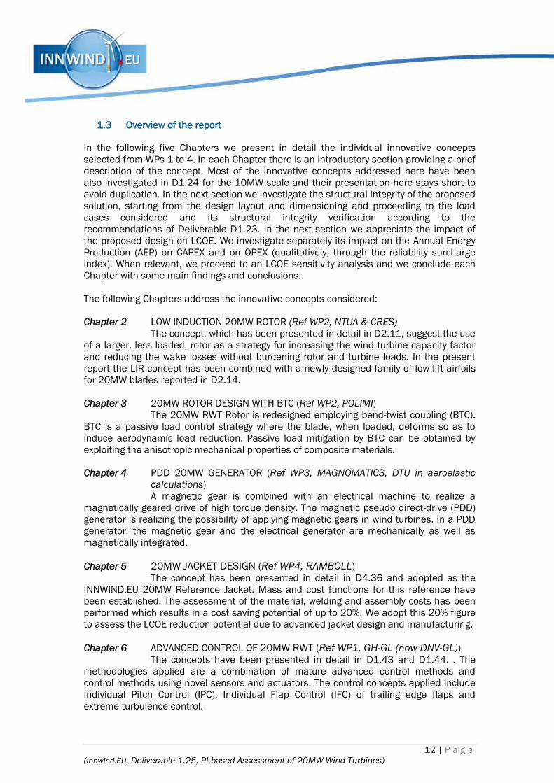
Figure 2.2-7 4th Mode Shape of 20MW LIR blade
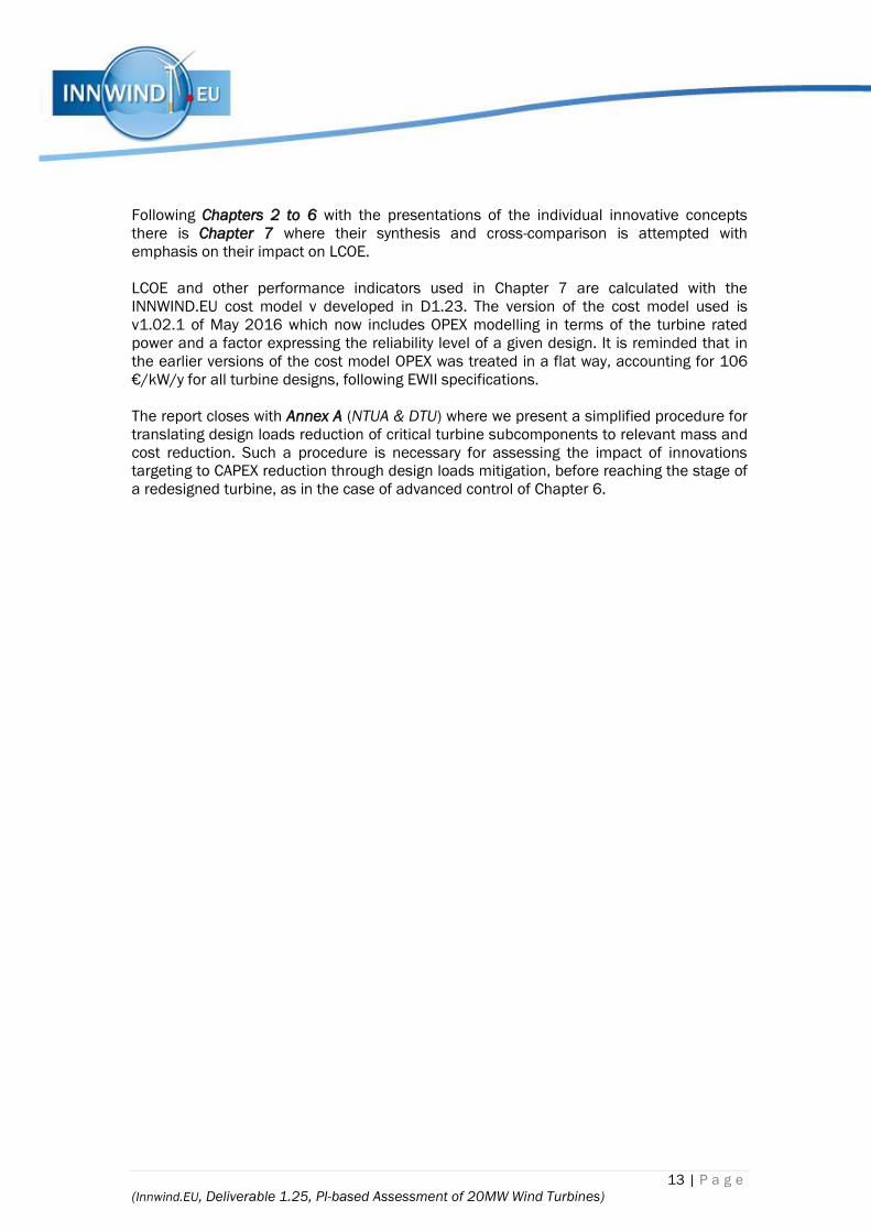
Figure 2.2-8 5th Mode Shape of 20MW LIR blade
Buckling analysis was performed considering safety factors for the stiffness properties of
the glass and carbon fabrics as also done within the benchmark. More specifically, the
values of the stiffness properties were divided by a factor 2.042. The value of the factor
was adopted following GL requirements. The first critical buckling load factor was
calculated equal to 0.74 while the respective eigen-mode is presented in Figure 2.2-9. The
critical location comprises the suction side of the blade. More specifically, buckling is
observed in the spar cap region at the ca. 40% of the blade length. A direct comparison
with the reference blade (buckling load factor 0.78) indicates that the LIR blade buckling
behavior is comparable with the RTW one.
21 | P a g e
(Innwind.EU, Deliverable 1.25, PI-based Assessment of 20MW Wind Turbines)
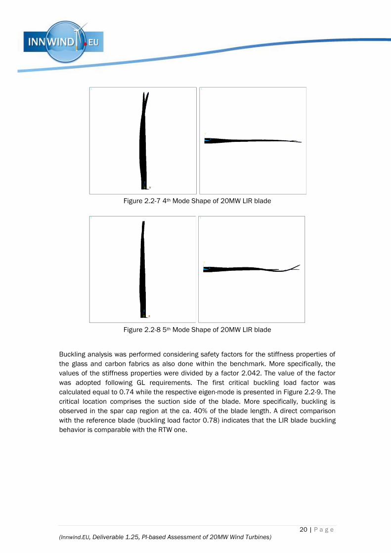
Figure 2.2-9 Buckling mode shape of the 20MW LIR blade
Strength analysis was performed calculating the Tsai-Wu failure index. Contour plots of the
maximum Tsai-Wu value among the various layers for every element is presented in Figure
2.2-10. Critical part of the blade comprises the suction side near the spar cap close to the
blade root with a failure index of 1.14. Reminding that the INNWIND.EU 20MW RWT
reference blade indicated a maximum Tsai-Wu failure index equal to 4.03 (using CRES
calculations), the current blade design is considered adequate. In Table 2.2 strength
analysis results are presented in terms of the strength multiplication factor as defined in
the benchmark study.

22 | P a g e
(Innwind.EU, Deliverable 1.25, PI-based Assessment of 20MW Wind Turbines)
Figure 2.2-9 Detailed distribution of Tsai-Wu failure index of 20 MW LIR blade
The design of the LIR blade that complies with structural integrity requirements resulted in
a lighter blade design compared to the reference one while the ratio of the carbon-layer
mass to the overall blade mass is 45.6%. An overall summary is presented in Table 2.2.
23 | P a g e
(Innwind.EU, Deliverable 1.25, PI-based Assessment of 20MW Wind Turbines)
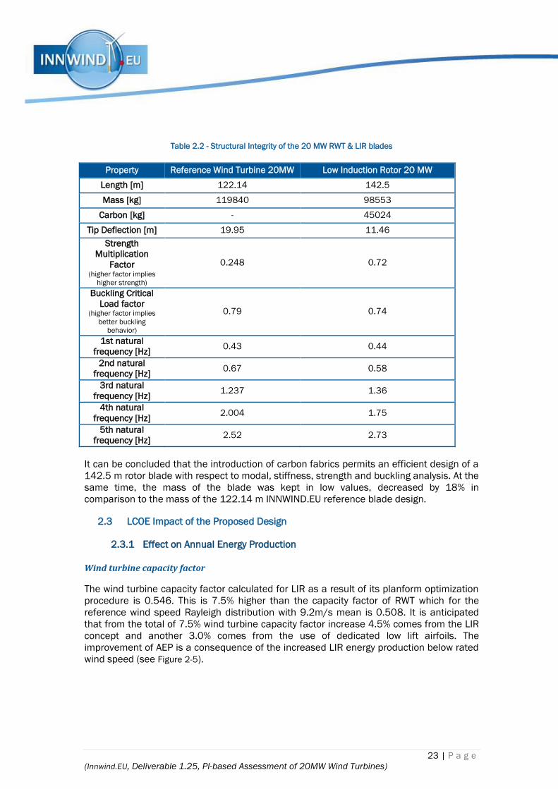
Table 2.2 - Structural Integrity of the 20 MW RWT & LIR blades
Property Reference Wind Turbine 20MW Low Induction Rotor 20 MW
Length [m] 122.14 142.5
Mass [kg] 119840 98553
Carbon [kg] - 45024
Tip Deflection [m] 19.95 11.46
Strength
Multiplication
Factor (higher factor implies
higher strength)
0.248 0.72
Buckling Critical
Load factor (higher factor implies
better buckling
behavior)
0.79 0.74
1st natural
frequency [Hz] 0.43 0.44
2nd natural
frequency [Hz] 0.67 0.58
3rd natural
frequency [Hz] 1.237 1.36
4th natural
frequency [Hz] 2.004 1.75
5th natural
frequency [Hz] 2.52 2.73
It can be concluded that the introduction of carbon fabrics permits an efficient design of a
142.5 m rotor blade with respect to modal, stiffness, strength and buckling analysis. At the
same time, the mass of the blade was kept in low values, decreased by 18% in
comparison to the mass of the 122.14 m INNWIND.EU reference blade design.
2.3 LCOE Impact of the Proposed Design
2.3.1 Effect on Annual Energy Production
Wind turbine capacity factor
The wind turbine capacity factor calculated for LIR as a result of its planform optimization
procedure is 0.546. This is 7.5% higher than the capacity factor of RWT which for the
reference wind speed Rayleigh distribution with 9.2m/s mean is 0.508. It is anticipated
that from the total of 7.5% wind turbine capacity factor increase 4.5% comes from the LIR
concept and another 3.0% comes from the use of dedicated low lift airfoils. The
improvement of AEP is a consequence of the increased LIR energy production below rated
wind speed (see Figure 2-5).

24 | P a g e
(Innwind.EU, Deliverable 1.25, PI-based Assessment of 20MW Wind Turbines)
Figure 2-5 Power and variable speed schedule (as Tip-Speed-Ratio) versus wind speed The LIR design
is considered with the low lift profiles family
Wind farm wakes
As already discussed in [3], LIRs are operating with reduced wake losses due to their lower
thrust coefficients. The calculations presented in [3] support a reduction of the wind farm
wake losses from 7% for the RWT to 5% for LIR, an improvement which directly reflects to
the wind farm capacity factor as well.
Other wind farm losses including availability losses
We do not expect the LIR to affect the reliability of the turbine and, therefore, its
availability losses.
2.3.2 Effect on CAPEX
Using a LIR instead of the original one of the 20MW RWT is affecting the CAPEX of the
following turbine subcomponents
Blades
As already discussed the need for stiffening the longer blade of the LIR to limit its
maximum deflection and trim its natural frequencies is satisfied by replacing the original
all-glass blade with a hybrid one with carbon spar. This necessitates the development of a
cost model for hybrid blades, given the fact that carbon fibre is three times more
expensive than glass fibre.
The cost figures used for the 20MW LIR blade derive from the cost model developed for
the hybrid 10MW LIR blade in [9]. The method involves the estimation of the baseline cost
of a full glass blade and then correcting the cost estimation by the ratio of carbon fiber
cost over glass cost. The method is well described in D1.24.
Firstly, the baseline blade cost is calculated:
Baseline blade cost: 13.084*98553-4452.2 = 1,285,015 $ (2002)

25 | P a g e
(Innwind.EU, Deliverable 1.25, PI-based Assessment of 20MW Wind Turbines)
It should be noted that CRES has estimated a weight for the reference blade of 119,840kg
instead of the 117,849Kg reported for the reference wind turbine. Therefore, a correction
for the weight estimation is done multiplying mass data by 0.9834. Correcting the baseline
blade cost the blade cost assuming all glass manufacturing is 1,263,663 $(2002).
The material cost ratio estimated for a rotor of 100.758m is: 50.95%
From the carbon layer mass provided the carbon fibres are estimated to 45,024 kg,
leading to a ratio over the whole blade mass of about 30.16%. When recalculating to
percentage of fibres, the carbon fibres used comprise the 50.26% of the total fibres.
Moreover, it is assumed that the carbon fibres cost 3 times as much as the glass fibres
and the percentage of fibers within the weight of the blade is ca. 60%.
Based on the above, the correction factor to be applied on the baseline cost estimated is:
(1-0.5095)+0.5095*(1-0.6)+0.5095*0.6*(1-0.5026)+0.5095*0.6*0.5026*3 = 1.307
Therefore, the cost of the hybrid glass/carbon blade is calculated to: 1,651,971 $(2002)
Tower
The LIR blade is 13% longer than the RWT one. However the 20MW RWT had already a
longer tower than needed to maintain the acceptable minimum blade-sea surface
distance. The longer tower of the RWT resulted from the need to reduce the first system’s
global frequency to avoid 3P excitation. The 20MW RWT tower is long enough to
accommodate the longer LIR blade without further modification.
LIR tower mass = RWT tower mass = 1.780t
LIR tower cost = RWT tower cost = 5.85 M€ (2012)
Offshore Support Structure
It is anticipated that the static loads of the offshore support structure will be reduced due
to the reduced rotor thrust. Nevertheless we have seen that such a reduction is not there
for the fatigue loads that drive the jacket design. We shall therefore assume that no
changes to the 20MW reference support structure are needed.
Other components
There is a small influence of LIR to other components CAPEX, such as the low speed shaft
or the yaw mechanism due to the increasing rotor size. These extra costs are automatically
taken into account by the INNWIND.EU cost model [10].
2.3.3 Effect on OPEX
Direct O&M costs, expressed in (€/kW/y) units are not affected by the introduction of LIR.
At the same time we do not anticipate any LIR consequences on the turbine availability.
Therefore, the replacement of the reference rotor with the LIR doesn’t have any positive or
negative effect on OPEX.

26 | P a g e
(Innwind.EU, Deliverable 1.25, PI-based Assessment of 20MW Wind Turbines)
2.4 Performance Indicators of 20MW LIR versus 20MW RWT
The comparison of LIR against the RWT in terms of key Performance Indicators is
presented in the following Table.
ROTOR Blade Mass
(tn) Blade Cost (k€ 2012)
Overall CAPEX
(k€) Turbine
CF
Wind Farm
CF LCOE
(€/MWh)
RWT - 20MW 118 1,274 68,000 0.508 0.437 96.50
LIR – 20MW 99 1,367 70,200 0.546 0.480 92.57
2.5 Conclusions
A 20 MW Low Induction Rotor has been designed aerodynamically and structurally. The
rotor is tested on the 20MW RWT platform of INNWIND.EU. A hybrid glass-carbon has
replaced the original all-glass blade of the RWT. The LIR is 13% longer and the hybrid
design aims in increasing the extra requirements for stiffness and strength dye to the
larger span. The hybrid blade:
Has 16% lower mass than the (up-scaled) 20MW RWT blade
Costs 7.3% more than the RWT blade
Has a wind turbine capacity factor 7.5% higher than the RWT blade
Yields a wind farm capacity factor 9.8% higher than the RWT blade due to the
reduced wake losses corresponding to the lower thrust coefficient of the LIR
Although the turbine CAPEX increases by 3.2% the overall effect of LIR on LCOE is quite
positive reducing it by 4.1%. The sensitivity of LCOE to the blade cost is relatively low. It is
shown however that if a new LIR blade can be designed with the same cost of the RWT
blade the LCOE would drop at 92.17 €/MWh.

27 | P a g e
(Innwind.EU, Deliverable 1.25, PI-based Assessment of 20MW Wind Turbines)
CHAPTER 3 20MW BLADE DESIGN WITH BTC
In this activity, a series of preliminary design studies have been conducted in order to
optimize the Key Performance Indicators (KPI) of a 20 MW reference wind turbine. The
starting point of the optimization process is the Baseline 20 MW developed by PoliMI for
Deliverable 2.14. This configuration was obtained as part of a mass-minimizing solution,
whose aim was to mimic as much as possible the aero-elastic properties of the 20MW
RWT [1] the rotor of which was obtained throughout up-scaling from 10MW. As discussed
in the corresponding report, this led to the design of a feasible structural layout for a given
aerodynamic shape, which fulfils fundamental integrity constraints formulated in
accordance with standard certification guidelines.
From here, we have performed a sequence of design steps in which several features of the
rotor are optimized in order to reduce as much as possible the total blade mass as well as
the ultimate and fatigue loads experienced by the turbine during its operational lifetime. In
particular, the introduction of a geometric rotation in the alignment of the spar caps fibres
(F-BTC) is exploited to significantly alleviate fundamental load figures, thanks to the
introduction of a structural coupling between the out-of-plane deflection of the blade and
its torsional deformation. Besides, other characteristics of the blade are optimized,
including the rotor solidity and its prebend, so that the combination of the structural
tailoring and the design refinements leads to additional aero-structural advantages in
terms of mass, AEP and LCOE.
3.1 Introduction to the Innovative Concept
There is strong evidence in the literature that the anisotropic properties of composite
laminates can be exploited to introduce desired behaviours in the dynamic response of
rotor blades. This process of structural tailoring has been reported for example by [11]
[12] [13] [14], while PoliMI presented a detailed application of a fiber-induced bend/twist
coupling (F-BTC) to the structural design of the INNWIND.EU 10 MW Baseline during the
Deliverable 2.22 [15] which resulted in significant load alleviations and related design
advantages.
Figure 3-1 Detail of a typical blade section with F-BTC

28 | P a g e
(Innwind.EU, Deliverable 1.25, PI-based Assessment of 20MW Wind Turbines)
In its general implementation, this technique can be exploited by introducing a certain
rotation in the lamination of the composites associated to the different structural
components, whereas the strongest beneficial effects are obtained when the fibers of the
spar caps are rotated, as shown in Figure 3-1. From a structural perspective, the main
consequence of the F-BTC is a modification of the fully-populated 6x6 stiffness matrix. In
particular, the extra-diagonal term which takes into account the flapwise displacement and
the torsional deformation, referred as KFlap/Tors is different from zero, as shown in Figure
3-2 (left) for the INNWIND.EU 10 MW rotor. It is evident how the magnitude of the KFlap/Tors
term is positively correlated with the amount of fiber orientation, which means that larger
rotations are associated to a stronger coupling effect. The same behaviour can be
quantified by looking at the non-dimensional coupling factor αBTC, which can be directly
computed from the stiffness matrix members as follows:
𝛼𝐵𝑇𝐶 = |𝑘𝐹𝑙𝑎𝑝/𝑇𝑜𝑟𝑠|
√𝐾𝐹𝑙𝑎𝑝 ∗ 𝐾𝑇𝑜𝑟𝑠
The corresponding spanwise distribution of the αBTC factor is illustrated for a varying
amount of fiber orientation in Figure 3-2 (right), which confirms that a stronger effect is
obtained for a larger amount of fiber rotation.
Figure 3-2 Flap/torsion stiffness and nondimensional BTC factor
The resulting effect is a built-in load alleviation mechanism: due to the non-zero extra-
diagonal stiffness term, when the blade bends in the flapwise direction, part of the
deformation energy is transformed into additional blade torsion. When the rotation of the
fibers is properly tuned, an out-of-plane deformation towards the suction side of the blade
results in a nose-in-the-wind rotation of the section, and therefore, the effective angle of
attack is automatically reduced resulting in lower loads. This can be checked by recurring
to simplified load cases.
29 | P a g e
(Innwind.EU, Deliverable 1.25, PI-based Assessment of 20MW Wind Turbines)
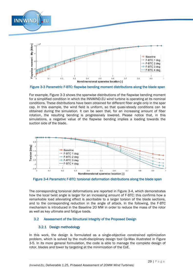
Figure 3-3 Parametric F-BTC: flapwise bending moment distributions along the blade span
For example, Figure 3-3 shows the spanwise distributions of the flapwise bending moment
for a simplified condition in which the INNWIND.EU wind turbine is operating at its nominal
conditions. These distributions have been obtained for different fiber angle only in the spar
cap. In this example, the wind field is uniform, so that quasi-steady conditions can be
obtained during the simulation. It can be seen that, for an increasing amount of fiber
rotation, the resulting bending is progressively lowered. Please notice that, in this
simulations, a negative value of the flapwise bending implies a loading towards the
suction side of the blade.
Figure 3-4 Parametric F-BTC: torsional deformation distributions along the blade span
The corresponding torsional deformations are reported in Figure 3-4, which demonstrates
how the local twist angle is larger for an increasing amount of F-BTC: this confirms how a
remarkable load alleviating effect is ascribable to a larger torsion of the blade sections,
and to the corresponding reduction in the angle of attack. In the following, the F-BTC
mechanism is introduced in the Baseline 20 MW in order to reduce the mass of the rotor
as well as key ultimate and fatigue loads.
3.2 Assessment of the Structural Integrity of the Proposed Design
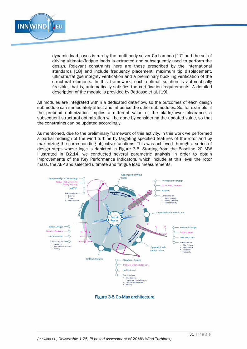
3.2.1 Design methodology
In this work, the design is formulated as a single-objective constrained optimization
problem, which is solved by the multi-disciplinary design tool Cp-Max illustrated in Figure
3-5. In its more general formulation, the code is able to manage the complete design of
rotor, blades and tower by targeting at the minimization of the CoE.
30 | P a g e
(Innwind.EU, Deliverable 1.25, PI-based Assessment of 20MW Wind Turbines)
As described by Bortolotti et al. [16] the architecture of the code is based on a continuous
interface among a primary (macro) loop, which handles the design of high-level
characteristics of the machine like radius, solidity, cone and tilt angles and several
submodules. These are responsible to conduct the detailed design of a specified
subsystem in order to optimize certain performance of the wind turbine. It must be noticed
that the mechanism is based on different nested optimization cycles so that, for each
variation of the macro parameters, an entire loop of the sub-modules is required.
According to the needs, Cp-Max can be run as an integrated design tool, in which the
macro design variables are sized through a full cycle of the underlying submodules.
Otherwise, it is possible to bypass the macro loop and run the required submodules as
standalone tools. This way, it is possible to save significant computational time where only
certain aspects of the design should be investigated.
The main submodules employed in these activities are briefly described in the following:
Aerodynamic design submodule:
This module performs the optimization of the chord, twist and non-dimensional
thickness (t/c) distributions along the blade. All quantities are described by means
of a suitable parameterization, whose nodal points are the design variables of a
dedicated optimization problem. The problem is solved by an SQP gradient-descent
method, which targets at the maximization of the theoretical AEP. This is obtained
through the computation of the Cp-TSR curves, which rapidly allow defining the
regulation trajectory of the machine, and thus the ideal AEP. Possible constraints
of this module include maximum chord and twist, as well as prescribed regularity
of the distributions. The rotor solidity is also a constraint for the aerodynamic
design submodule: if a solidity value is specified, the chord distribution is design to
satisfy this value.
Prebend design submodule:
This module is able to perform the design of the prebend distribution along the
blade. This is suitably discretized by means of Bézier curves, whose control points
are the unknowns of a dedicated optimization problem. Here, the goal of the
optimization is to design the prebend such that the deformed rotor area at rated
conditions is maximized. This also represents an indirect requirement on the
maximization (or at least preservation) of the AEP, under the assumptions that the
effective disk area is directly correlated to the energy yielding of the wind turbine.
Constraints can be imposed on the shape regularity, as well as on the maximum
value of the prebend, which is usually determined by technological and
manufacturing limitations.
Structural design submodule:
This module allows optimizing the total blade mass by sizing the thickness of all
the structural elements along the blade. The design variables account for the
thickness of all the composite fabrics (i.e. unidirectional, biaxial, triaxial) and that
of the fillers (core, balsa, foam) so that a complete structural description of the
blade is achieved at the end of the process. Ahead of the optimization, a set of
31 | P a g e
(Innwind.EU, Deliverable 1.25, PI-based Assessment of 20MW Wind Turbines)
dynamic load cases is run by the multi-body solver Cp-Lambda [17] and the set of
driving ultimate/fatigue loads is extracted and subsequently used to perform the
design. Relevant constraints here are those prescribed by the international
standards [18] and include frequency placement, maximum tip displacement,
ultimate/fatigue integrity verification and a preliminary buckling verification of the
structural elements. In this framework, each optimal solution is automatically
feasible, that is, automatically satisfies the certification requirements. A detailed
description of the module is provided by Bottasso et al. [19].
All modules are integrated within a dedicated data-flow, so the outcomes of each design
submodule can immediately affect and influence the other submodules. So, for example, if
the prebend optimization implies a different value of the blade/tower clearance, a
subsequent structural optimization will be done by considering the updated value, so that
the constraints can be updated accordingly.
As mentioned, due to the preliminary framework of this activity, in this work we performed
a partial redesign of the wind turbine by targeting specified features of the rotor and by
maximizing the corresponding objective functions. This was achieved through a series of
design steps whose logic is depicted in Figure 3-6. Starting from the Baseline 20 MW
illustrated in D2.14, we conducted several parametric analysis in order to obtain
improvements of the Key Performance Indicators, which include at this level the rotor
mass, the AEP and selected ultimate and fatigue load measurements.
Figure 3-5 Cp-Max architecture
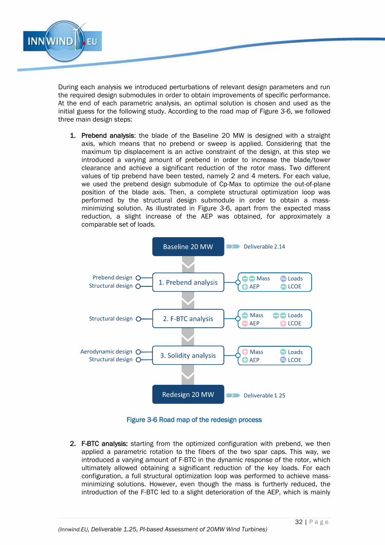
32 | P a g e
(Innwind.EU, Deliverable 1.25, PI-based Assessment of 20MW Wind Turbines)
During each analysis we introduced perturbations of relevant design parameters and run
the required design submodules in order to obtain improvements of specific performance.
At the end of each parametric analysis, an optimal solution is chosen and used as the
initial guess for the following study. According to the road map of Figure 3-6, we followed
three main design steps:
1. Prebend analysis: the blade of the Baseline 20 MW is designed with a straight
axis, which means that no prebend or sweep is applied. Considering that the
maximum tip displacement is an active constraint of the design, at this step we
introduced a varying amount of prebend in order to increase the blade/tower
clearance and achieve a significant reduction of the rotor mass. Two different
values of tip prebend have been tested, namely 2 and 4 meters. For each value,
we used the prebend design submodule of Cp-Max to optimize the out-of-plane
position of the blade axis. Then, a complete structural optimization loop was
performed by the structural design submodule in order to obtain a mass-
minimizing solution. As illustrated in Figure 3-6, apart from the expected mass
reduction, a slight increase of the AEP was obtained, for approximately a
comparable set of loads.
Figure 3-6 Road map of the redesign process
2. F-BTC analysis: starting from the optimized configuration with prebend, we then
applied a parametric rotation to the fibers of the two spar caps. This way, we
introduced a varying amount of F-BTC in the dynamic response of the rotor, which
ultimately allowed obtaining a significant reduction of the key loads. For each
configuration, a full structural optimization loop was performed to achieve mass-
minimizing solutions. However, even though the mass is furtherly reduced, the
introduction of the F-BTC led to a slight deterioration of the AEP, which is mainly

33 | P a g e
(Innwind.EU, Deliverable 1.25, PI-based Assessment of 20MW Wind Turbines)
related to the larger torsional flexibility which makes the blade sections to operate
away from the optimal aerodynamic efficiency.
3. Solidity analysis: In the last step of the design process, we started from the
coupled F-BTC rotor designed at the previous step and progressively reduced the
rotor solidity. For each value of solidity, we performed a redesign of the chord and
twist distributions through the aerodynamic design submodule, in order to obtain
AEP-maximizing solutions. Again, each configuration was then structurally
optimized by the structural design submodule of Cp-Max. At this stage, we obtain a
further reduction of the key loads, even though the lower solidity required a higher
mass of the structural components. However, the AEP was globally increased so
that approximately the same LCOE is achieved for all the parametric solutions.
3.2.2 Design assumptions
Structural Layout
All the solutions are based on the structural arrangement described in D2.14. The internal
layout is shown in Figure 3-7, and is based on the common spar-box concept. The width
and positions of all the sectional elements was kept as frozen during the entire design
activity, while the thickness of the sectional components are recursively optimized by
means of the structural design submodule of Cp-Max.
Figure 3-7 Sectional elements and structural components
Cost model
It is important to notice that we didn’t employ the LCOE as merit function during the design
process, since the main focus of the various steps was on the mass and loads mitigation.
However, we thoroughly assess the COE during the process, in order to identify possible
advantages in terms of cost reductions. In this activity, we computed the cost of energy

34 | P a g e
(Innwind.EU, Deliverable 1.25, PI-based Assessment of 20MW Wind Turbines)
according to the INNWIND.EU cost model described by Chaviaropoulos [10] . The main
assumptions that we adopted are the following:
Plant capacity: we assumed an ideal wind farm with only a single wind turbine. So,
the LCOE is directly computed for a unitary WT.
Blade cost: this was obtained from the total blade mass following the scaling law:
𝐵𝑙𝑎𝑑𝑒 𝑐𝑜𝑠𝑡 = 13.084 ∗ 𝐵𝑙𝑎𝑑𝑒 𝑚𝑎𝑠𝑠 − 4452.2
Tower cost: this was obtained from the total tower mass following the scaling law:
𝑇𝑜𝑤𝑒𝑟 𝑐𝑜𝑠𝑡 = 𝑇𝑜𝑤𝑒𝑟 𝑚𝑎𝑠𝑠 ∗ 4.35
Conversion: we assumed that 1 USD = 0.75758 EUR.
Actualization: we assumed a nominal discount rate of 0.0739 %
AEP: in this work we use the turbulent energy production, which is obtained as an
averaged measurement of the electrical power obtained during turbulent
simulations (DLC 1.1)
Capacity factor: for its estimation, we adopted the following simplified relation:
𝑐𝑓 =𝐴𝐸𝑃
8760 ∗ 𝑃𝑅𝑎𝑡𝑒𝑑
Control
During the whole design process we used the external controller provided by Hansen and
Henriksen (2013). The main settings/parameters were taken from the original datasheet
of the 20 MW reference wind turbine.
To account for the modifications investigated during the design process, for each solution
we defined an updated regulation trajectory. This was basically done by computing the
envelope of the Cp-TSR curves ahead of the structural optimization loop. Subsequently, we
computed the ideal rotor speed and a suitable pitch-scheduling look-up table. That
information was then supplied to the controller, so that each configuration can operate
close to its theoretical optimal point.
3.2.3 Load cases considered
Due to the significant amount of configurations investigated in this work, we used a basic
set of DLC, which are defined according to IEC standards. The list of considered DLC is
provided in Table 3-1 together with the corresponding definition and safety factors for the
computation of the ultimate sizing loads. The list includes cases in normal operations as
well as selected gust conditions, faults and storm situations. For the turbulent simulations
only one seed was considered in order to save computational time. All turbulent winds
were generated in accordance to the required wind turbine class through the Kaimal
model.

35 | P a g e
(Innwind.EU, Deliverable 1.25, PI-based Assessment of 20MW Wind Turbines)
Table 3-1 List of considered DLC
DLC Wind No. of
Seeds Wind speed Yaw mis. Fault SF
1.1 NTM 1 vIN : vOUT - - 1.35
1.3 ETM 1 vIN : vOUT - - 1.35
2.1 NTM 1 vIN : vOUT - Grid loss 1.35
2.3 EOG Vr-2 , vr , vr+2 ,
vOUT - Grid loss 1.1
6.1 EWM 1 vREF -8°: 8° - 1.35
6.2 EWM 1 vREf 180°:
180° Grid loss 1.1
3.2.4 Parametric design results
In this paragraph, we provide fundamental results for each step of the design process
described in the previous section. The investigated performances are ultimate and fatigue
loads, the turbulent AEP, the total blade mass and the LCOE. It must be noticed that all the
results are given as percent variation against the optimal solution identified at the
previous step. Results of the first design step, on the contrary, are given as percent
variation against the PoliMI Baseline 20 MW.
Step 1 - Prebend analysis
Starting from the PoliMI Baseline 20 MW, initially a parametric prebend was applied to the
geometric description of the blade axis, in order to increase the blade/tower clearance
and to relieve the maximum tip displacement constraint which drives the structural design
of the initial solution. Configurations with a maximum prebend at tip of 2m and 4m were
investigated, and each distribution was optimally designed by the dedicated submodule of
Cp-Max. The final shapes are illustrated for both solutions in Figure 3-8.
Figure 3-8 Step 1: optimal prebend distributions
The impact on the global performance is somewhat expected, and the main findings are
summarized in Figure 3-9, which shows percent variations of total blade mass, AEP and
LCOE of the two solutions with prebend against the Baseline 20 MW. As anticipated, the
larger clearance ensures that a lighter blade can be designed for the same constraints,
leading to a decrease of the blade mass. According to the formulation of the prebend
optimization problem, the AEP is slightly increased in both cases, even though the huge

36 | P a g e
(Innwind.EU, Deliverable 1.25, PI-based Assessment of 20MW Wind Turbines)
flexibility associated to a larger prebend in part limits the energy gain. However, the LCOE
predicted by the INNWIND.EU model is reduced in both cases.
Figure 3-9 Step 1: performance variations against the PoliMI Baseline 20 MW
The percent variation of key ultimate and fatigue loads are provided in Figure 3-10 against
the PoliMI Baseline 20 MW. Please notice that the first four dataset refer to ultimate loads,
while the right-most columns represent fatigue DEL.
When ultimate loads are considered, they are expressed as the multi-directional
‘combined’ bending at each component. So, for example, the blade root bending refers to
the composed flapwise/edgewise bending, whose magnitude is usually higher than the
individual load components. The same applies to the hub, where the yawing/nodding
bending is considered and to the tower, where the combined fore-aft/side-side is shown.
Figure 3-10 Step 1: ultimate and fatigue loads variations against the Baseline 20 MW
The results show that, with the exception of the tower base FA DEL, all key loads are
encompassed in a range of approximately +/- 5% when compared against the baseline.
Since the Prebend – 4m solution produces lower loads, it is considered the best one and
used as starting point for the next step.
Step 2 – F-BTC Analysis
In the second step of the design procedure, we applied a parametric rotation to the fibers
of the spar caps, in order to trigger the F-BTC mitigating effect. Three different
configurations corresponding to rotations of 4, 6 and 8 degrees have been tested. Figure
3-12 gives the percent variation of the performance indicators against the Prebend – 4m
solution, showing that an additional 2% of mass reduction can be achieved for the F-BTC 6
deg solution.
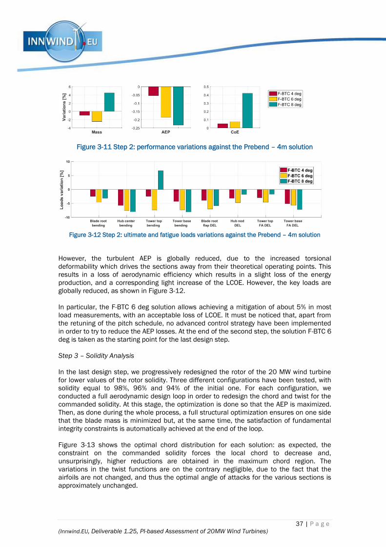
37 | P a g e
(Innwind.EU, Deliverable 1.25, PI-based Assessment of 20MW Wind Turbines)
Figure 3-11 Step 2: performance variations against the Prebend – 4m solution
Figure 3-12 Step 2: ultimate and fatigue loads variations against the Prebend – 4m solution
However, the turbulent AEP is globally reduced, due to the increased torsional
deformability which drives the sections away from their theoretical operating points. This
results in a loss of aerodynamic efficiency which results in a slight loss of the energy
production, and a corresponding light increase of the LCOE. However, the key loads are
globally reduced, as shown in Figure 3-12.
In particular, the F-BTC 6 deg solution allows achieving a mitigation of about 5% in most
load measurements, with an acceptable loss of LCOE. It must be noticed that, apart from
the retuning of the pitch schedule, no advanced control strategy have been implemented
in order to try to reduce the AEP losses. At the end of the second step, the solution F-BTC 6
deg is taken as the starting point for the last design step.
Step 3 – Solidity Analysis
In the last design step, we progressively redesigned the rotor of the 20 MW wind turbine
for lower values of the rotor solidity. Three different configurations have been tested, with
solidity equal to 98%, 96% and 94% of the initial one. For each configuration, we
conducted a full aerodynamic design loop in order to redesign the chord and twist for the
commanded solidity. At this stage, the optimization is done so that the AEP is maximized.
Then, as done during the whole process, a full structural optimization ensures on one side
that the blade mass is minimized but, at the same time, the satisfaction of fundamental
integrity constraints is automatically achieved at the end of the loop.
Figure 3-13 shows the optimal chord distribution for each solution: as expected, the
constraint on the commanded solidity forces the local chord to decrease and,
unsurprisingly, higher reductions are obtained in the maximum chord region. The
variations in the twist functions are on the contrary negligible, due to the fact that the
airfoils are not changed, and thus the optimal angle of attacks for the various sections is
approximately unchanged.
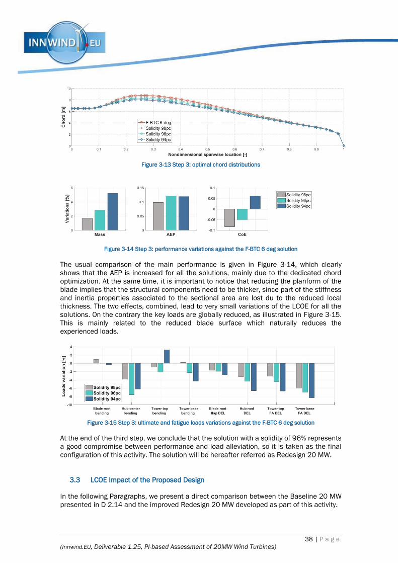
38 | P a g e
(Innwind.EU, Deliverable 1.25, PI-based Assessment of 20MW Wind Turbines)
Figure 3-13 Step 3: optimal chord distributions
Figure 3-14 Step 3: performance variations against the F-BTC 6 deg solution
The usual comparison of the main performance is given in Figure 3-14, which clearly
shows that the AEP is increased for all the solutions, mainly due to the dedicated chord
optimization. At the same time, it is important to notice that reducing the planform of the
blade implies that the structural components need to be thicker, since part of the stiffness
and inertia properties associated to the sectional area are lost du to the reduced local
thickness. The two effects, combined, lead to very small variations of the LCOE for all the
solutions. On the contrary the key loads are globally reduced, as illustrated in Figure 3-15.
This is mainly related to the reduced blade surface which naturally reduces the
experienced loads.
Figure 3-15 Step 3: ultimate and fatigue loads variations against the F-BTC 6 deg solution
At the end of the third step, we conclude that the solution with a solidity of 96% represents
a good compromise between performance and load alleviation, so it is taken as the final
configuration of this activity. The solution will be hereafter referred as Redesign 20 MW.
3.3 LCOE Impact of the Proposed Design
In the following Paragraphs, we present a direct comparison between the Baseline 20 MW
presented in D 2.14 and the improved Redesign 20 MW developed as part of this activity.
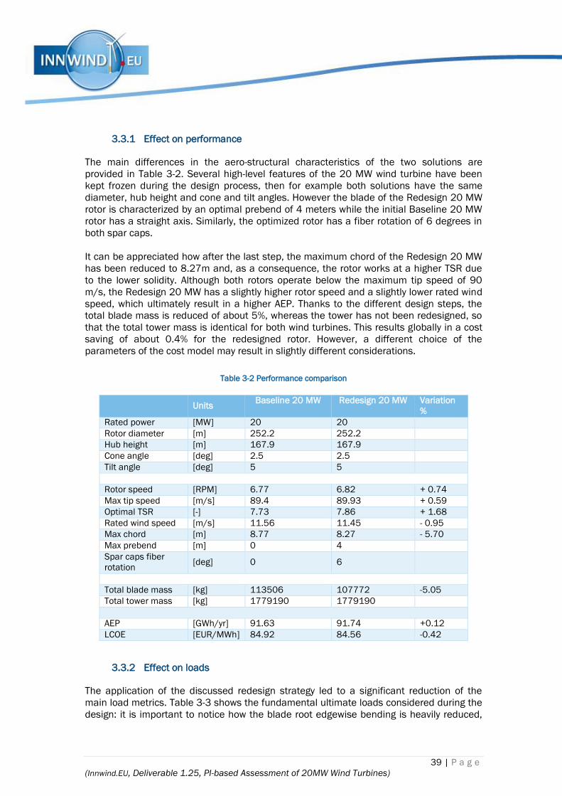
39 | P a g e
(Innwind.EU, Deliverable 1.25, PI-based Assessment of 20MW Wind Turbines)
3.3.1 Effect on performance
The main differences in the aero-structural characteristics of the two solutions are
provided in Table 3-2. Several high-level features of the 20 MW wind turbine have been
kept frozen during the design process, then for example both solutions have the same
diameter, hub height and cone and tilt angles. However the blade of the Redesign 20 MW
rotor is characterized by an optimal prebend of 4 meters while the initial Baseline 20 MW
rotor has a straight axis. Similarly, the optimized rotor has a fiber rotation of 6 degrees in
both spar caps.
It can be appreciated how after the last step, the maximum chord of the Redesign 20 MW
has been reduced to 8.27m and, as a consequence, the rotor works at a higher TSR due
to the lower solidity. Although both rotors operate below the maximum tip speed of 90
m/s, the Redesign 20 MW has a slightly higher rotor speed and a slightly lower rated wind
speed, which ultimately result in a higher AEP. Thanks to the different design steps, the
total blade mass is reduced of about 5%, whereas the tower has not been redesigned, so
that the total tower mass is identical for both wind turbines. This results globally in a cost
saving of about 0.4% for the redesigned rotor. However, a different choice of the
parameters of the cost model may result in slightly different considerations.
Table 3-2 Performance comparison
Units
Baseline 20 MW Redesign 20 MW Variation
%
Rated power [MW] 20 20
Rotor diameter [m] 252.2 252.2
Hub height [m] 167.9 167.9
Cone angle [deg] 2.5 2.5
Tilt angle [deg] 5 5
Rotor speed [RPM] 6.77 6.82 + 0.74
Max tip speed [m/s] 89.4 89.93 + 0.59
Optimal TSR [-] 7.73 7.86 + 1.68
Rated wind speed [m/s] 11.56 11.45 - 0.95
Max chord [m] 8.77 8.27 - 5.70
Max prebend [m] 0 4
Spar caps fiber
rotation [deg] 0 6
Total blade mass [kg] 113506 107772 -5.05
Total tower mass [kg] 1779190 1779190
AEP [GWh/yr] 91.63 91.74 +0.12
LCOE [EUR/MWh] 84.92 84.56 -0.42
3.3.2 Effect on loads
The application of the discussed redesign strategy led to a significant reduction of the
main load metrics. Table 3-3 shows the fundamental ultimate loads considered during the
design: it is important to notice how the blade root edgewise bending is heavily reduced,
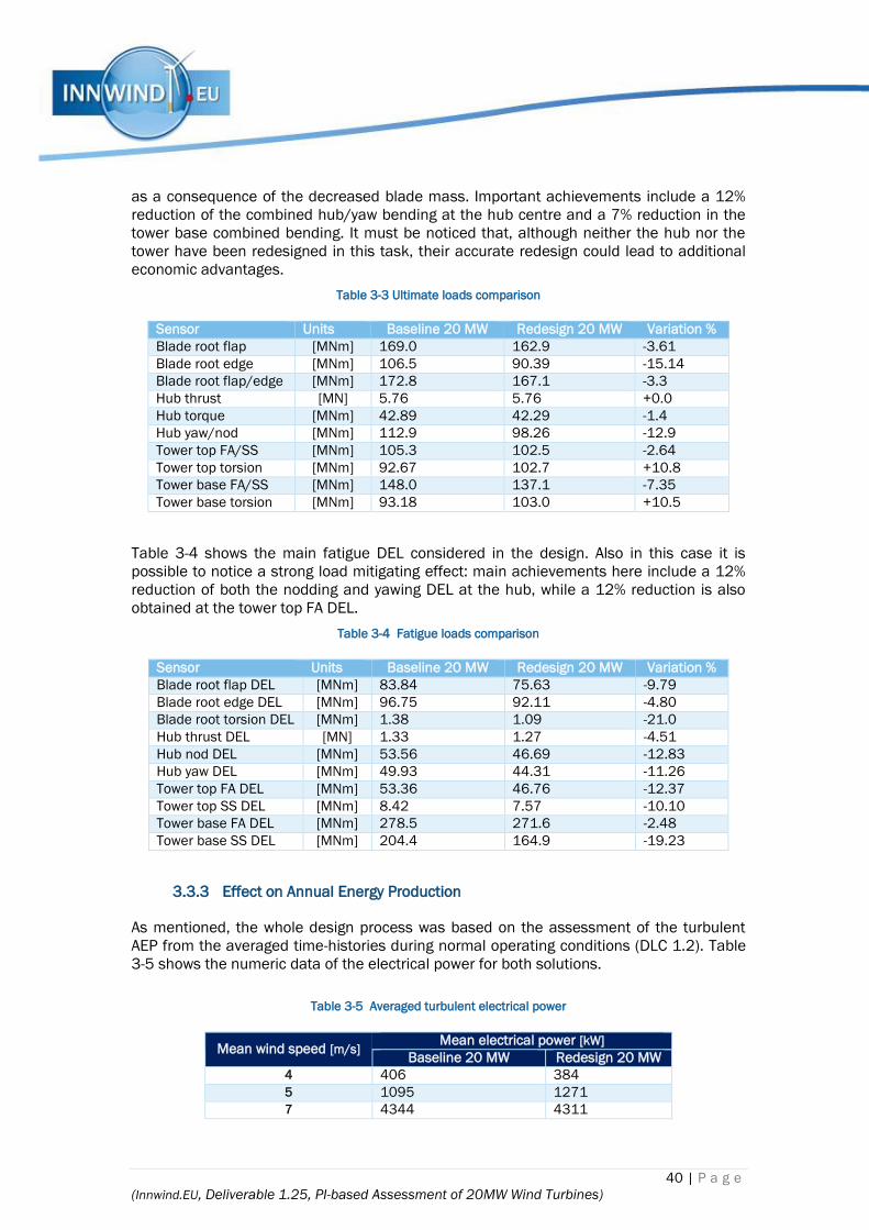
40 | P a g e
(Innwind.EU, Deliverable 1.25, PI-based Assessment of 20MW Wind Turbines)
as a consequence of the decreased blade mass. Important achievements include a 12%
reduction of the combined hub/yaw bending at the hub centre and a 7% reduction in the
tower base combined bending. It must be noticed that, although neither the hub nor the
tower have been redesigned in this task, their accurate redesign could lead to additional
economic advantages.
Table 3-3 Ultimate loads comparison
Sensor Units Baseline 20 MW Redesign 20 MW Variation %
Blade root flap [MNm] 169.0 162.9 -3.61
Blade root edge [MNm] 106.5 90.39 -15.14
Blade root flap/edge [MNm] 172.8 167.1 -3.3
Hub thrust [MN] 5.76 5.76 +0.0
Hub torque [MNm] 42.89 42.29 -1.4
Hub yaw/nod [MNm] 112.9 98.26 -12.9
Tower top FA/SS [MNm] 105.3 102.5 -2.64
Tower top torsion [MNm] 92.67 102.7 +10.8
Tower base FA/SS [MNm] 148.0 137.1 -7.35
Tower base torsion [MNm] 93.18 103.0 +10.5
Table 3-4 shows the main fatigue DEL considered in the design. Also in this case it is
possible to notice a strong load mitigating effect: main achievements here include a 12%
reduction of both the nodding and yawing DEL at the hub, while a 12% reduction is also
obtained at the tower top FA DEL.
Table 3-4 Fatigue loads comparison
Sensor Units Baseline 20 MW Redesign 20 MW Variation %
Blade root flap DEL [MNm] 83.84 75.63 -9.79
Blade root edge DEL [MNm] 96.75 92.11 -4.80
Blade root torsion DEL [MNm] 1.38 1.09 -21.0
Hub thrust DEL [MN] 1.33 1.27 -4.51
Hub nod DEL [MNm] 53.56 46.69 -12.83
Hub yaw DEL [MNm] 49.93 44.31 -11.26
Tower top FA DEL [MNm] 53.36 46.76 -12.37
Tower top SS DEL [MNm] 8.42 7.57 -10.10
Tower base FA DEL [MNm] 278.5 271.6 -2.48
Tower base SS DEL [MNm] 204.4 164.9 -19.23
3.3.3 Effect on Annual Energy Production
As mentioned, the whole design process was based on the assessment of the turbulent
AEP from the averaged time-histories during normal operating conditions (DLC 1.2). Table
3-5 shows the numeric data of the electrical power for both solutions.
Table 3-5 Averaged turbulent electrical power
Mean wind speed [m/s] Mean electrical power [kW]
Baseline 20 MW Redesign 20 MW
4 406 384
5 1095 1271
7 4344 4311
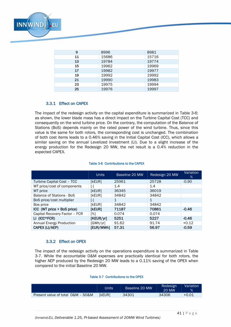
41 | P a g e
(Innwind.EU, Deliverable 1.25, PI-based Assessment of 20MW Wind Turbines)
9 8996 8981
11 15686 15716
13 19784 19774
15 19962 19969
17 19982 19977
19 19992 19992
21 19990 19983
23 19975 19994
25 19976 19997
3.3.1 Effect on CAPEX
The impact of the redesign activity on the capital expenditure is summarized in Table 3-6:
as shown, the lower blade mass has a direct impact on the Turbine Capital Cost (TCC) and
consequently on the wind turbine price. On the contrary, the computation of the Balance of
Stations (BoS) depends mainly on the rated power of the wind turbine. Thus, since this
value is the same for both rotors, the corresponding cost is unchanged. The combination
of both cost items leads to a 0.46% saving in the Initial Capital Cost (ICC), which allows a
similar saving on the annual Levelized Investment (LI). Due to a slight increase of the
energy production for the Redesign 20 MW, the net result is a 0.4% reduction in the
expected CAPEX.
Table 3-6 Contributions to the CAPEX
Units Baseline 20 MW Redesign 20 MW Variation
%
Turbine Capital Cost – TCC [kEUR] 25961 25728 -0.90
WT price/cost of components [-] 1.4 1.4
WT price [kEUR] 36345 36019
Balance of Stations - BoS [kEUR] 34842 34842
BoS price/cost multiplier [-] 1 1
Bos price [kEUR] 34842 34842
ICC (WT price + BoS price) [kEUR] 71187 70861 -0.46
Capital Recovery Factor – FCR [%] 0.074 0.074
LI (ICC*FCR) [KEUR/yr] 5251 5227 -0.46
Annual Energy Production [GWh/yr] 91.62 91.74 +0.12
CAPEX (LI/AEP) [EUR/MWh] 57.31 56.97 -0.59
3.3.2 Effect on OPEX
The impact of the redesign activity on the operations expenditure is summarized in Table
3-7. While the accountable O&M expenses are practically identical for both rotors, the
higher AEP produced by the Redesign 20 MW leads to a 0.11% saving of the OPEX when
compared to the initial Baseline 20 MW.
Table 3-7 Contributions to the OPEX
Units Baseline 20 MW Redesign
20 MW
Variation
%
Present value of total O&M – SO&M [kEUR] 34301 34306 +0.01

42 | P a g e
(Innwind.EU, Deliverable 1.25, PI-based Assessment of 20MW Wind Turbines)
Capital Recovery Factor – FCR [%] 0.074 0.074
Annual Discounted O&M – DO&M [kEUR/yr] 2530 2531 +0.04
Annual Energy Production [GWh/yr] 91.62 91.74
OPEX (DOE&M/AEP) [EUR/MWh] 27.61 27.58 -0.11
3.4 Conclusions
In this work, we performed a preliminary aero-structural redesign of the Baseline 20 MW
presented in the Deliverable 2.14. As part of the redesign activities, we conducted several
parametric studies in order to find a suitable design strategy which can improve the
performance of the Baseline 20 MW rotor.
In particular, we choose to concentrate on the load mitigation and on the total blade mass
reduction rather than on the reduction of the LCOE. This choice is mainly driven by the
significant ultimate and fatigue loads developed by the Baseline 20 MW, which make
recommendable to adopt suitable countermeasures in order to reduce the key loads as
much as possible. Future developments of this activity will focus on a proper cost-
minimization design loop.
The design process was based on three different steps in which the prebend, the spar cap
fiber rotation and the rotor solidity were investigated and optimized.
The resulting rotor shows a 5% reduction in the total blade mass while at the same time it
achieves significantly lower loads when compared against those developed by the
Baseline 20 MW. The final step led to an increase TSR which in turn ensure a slight
improvement of the AEP (when computed from DLC 1.2) and a 0.4% reduction of the
LCOE.
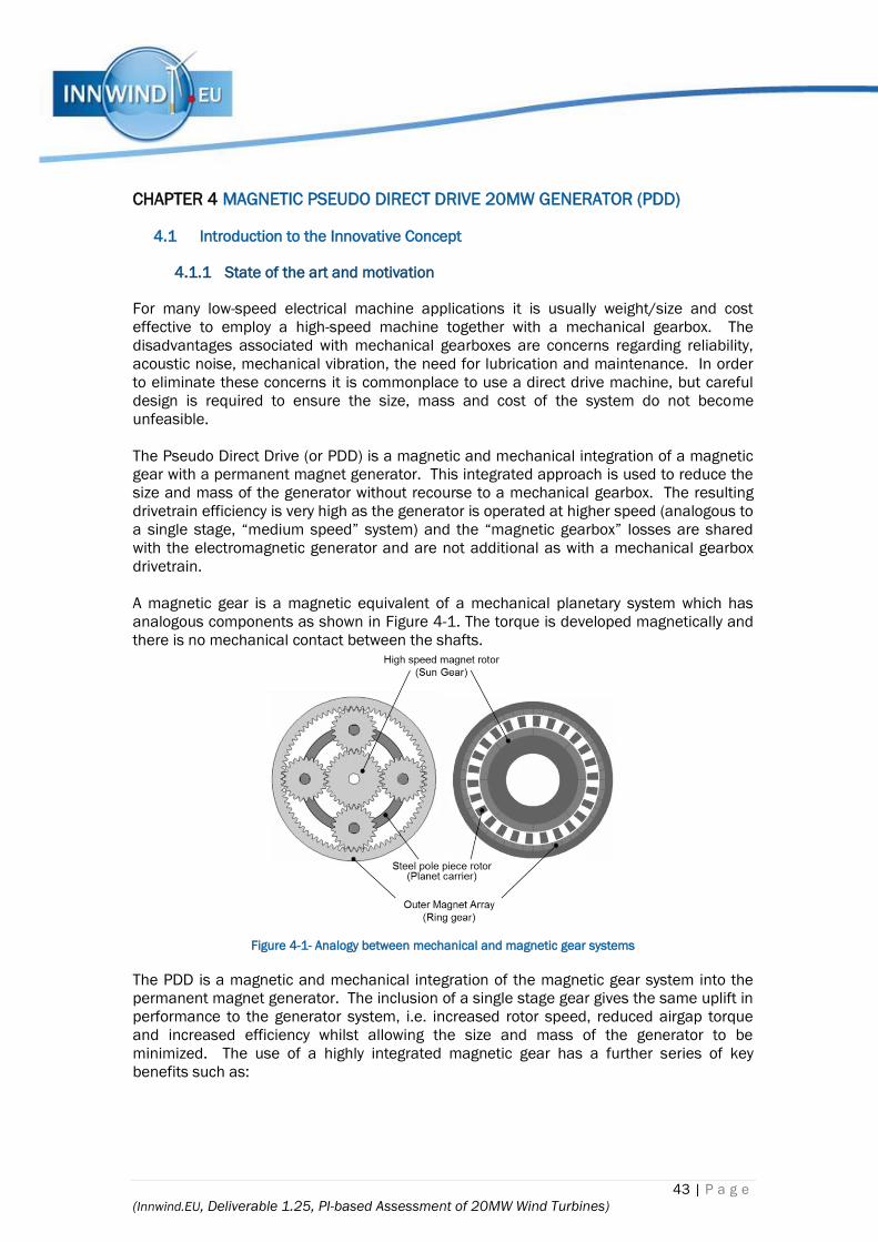
43 | P a g e
(Innwind.EU, Deliverable 1.25, PI-based Assessment of 20MW Wind Turbines)
CHAPTER 4 MAGNETIC PSEUDO DIRECT DRIVE 20MW GENERATOR (PDD)
4.1 Introduction to the Innovative Concept
4.1.1 State of the art and motivation
For many low-speed electrical machine applications it is usually weight/size and cost
effective to employ a high-speed machine together with a mechanical gearbox. The
disadvantages associated with mechanical gearboxes are concerns regarding reliability,
acoustic noise, mechanical vibration, the need for lubrication and maintenance. In order
to eliminate these concerns it is commonplace to use a direct drive machine, but careful
design is required to ensure the size, mass and cost of the system do not become
unfeasible.
The Pseudo Direct Drive (or PDD) is a magnetic and mechanical integration of a magnetic
gear with a permanent magnet generator. This integrated approach is used to reduce the
size and mass of the generator without recourse to a mechanical gearbox. The resulting
drivetrain efficiency is very high as the generator is operated at higher speed (analogous to
a single stage, “medium speed” system) and the “magnetic gearbox” losses are shared
with the electromagnetic generator and are not additional as with a mechanical gearbox
drivetrain.
A magnetic gear is a magnetic equivalent of a mechanical planetary system which has
analogous components as shown in Figure 4-1. The torque is developed magnetically and
there is no mechanical contact between the shafts.
Figure 4-1- Analogy between mechanical and magnetic gear systems
The PDD is a magnetic and mechanical integration of the magnetic gear system into the
permanent magnet generator. The inclusion of a single stage gear gives the same uplift in
performance to the generator system, i.e. increased rotor speed, reduced airgap torque
and increased efficiency whilst allowing the size and mass of the generator to be
minimized. The use of a highly integrated magnetic gear has a further series of key
benefits such as:
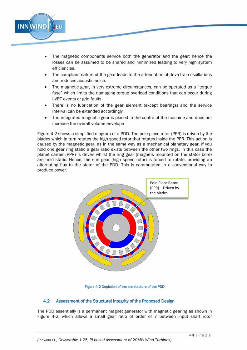
44 | P a g e
(Innwind.EU, Deliverable 1.25, PI-based Assessment of 20MW Wind Turbines)
The magnetic components service both the generator and the gear; hence the
losses can be assumed to be shared and minimized leading to very high system
efficiencies.
The compliant nature of the gear leads to the attenuation of drive train oscillations
and reduces acoustic noise.
The magnetic gear, in very extreme circumstances, can be operated as a “torque
fuse” which limits the damaging torque overload conditions that can occur during
LVRT events or grid faults.
There is no lubrication of the gear element (except bearings) and the service
interval can be extended accordingly
The integrated magnetic gear is placed in the centre of the machine and does not
increase the overall volume envelope
Figure 4-2 shows a simplified diagram of a PDD. The pole-piece rotor (PPR) is driven by the
blades which in turn rotates the high speed rotor that rotates inside the PPR. This action is
caused by the magnetic gear, as in the same way as a mechanical planetary gear, if you
hold one gear ring static a gear ratio exists between the other two rings. In this case the
planet carrier (PPR) is driven whilst the ring gear (magnets mounted on the stator bore)
are held static. Hence, the sun gear (high speed rotor) is forced to rotate, providing an
alternating flux to the stator of the PDD. This is commutated in a conventional way to
produce power.
Figure 4-2 Depiction of the architecture of the PDD
4.2 Assessment of the Structural Integrity of the Proposed Design
The PDD essentially is a permanent magnet generator with magnetic gearing as shown in
Figure 4-2, which allows a small gear ratio of order of 7 between input shaft rotor
Pole Piece Rotor (PPR) – Driven by the blades
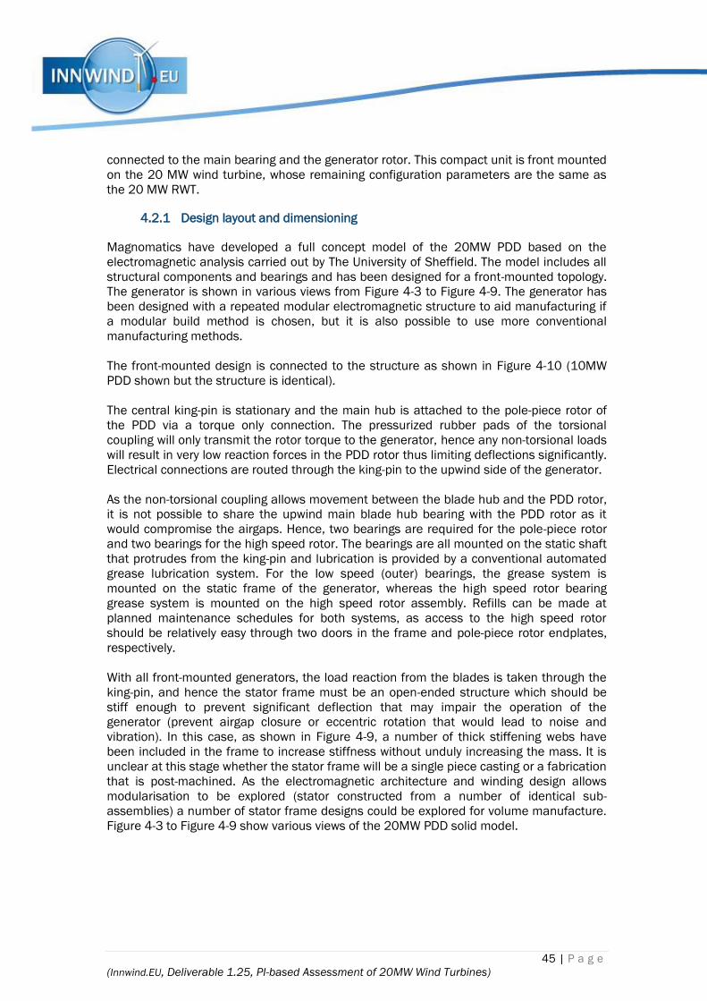
45 | P a g e
(Innwind.EU, Deliverable 1.25, PI-based Assessment of 20MW Wind Turbines)
connected to the main bearing and the generator rotor. This compact unit is front mounted
on the 20 MW wind turbine, whose remaining configuration parameters are the same as
the 20 MW RWT.
4.2.1 Design layout and dimensioning
Magnomatics have developed a full concept model of the 20MW PDD based on the
electromagnetic analysis carried out by The University of Sheffield. The model includes all
structural components and bearings and has been designed for a front-mounted topology.
The generator is shown in various views from Figure 4-3 to Figure 4-9. The generator has
been designed with a repeated modular electromagnetic structure to aid manufacturing if
a modular build method is chosen, but it is also possible to use more conventional
manufacturing methods.
The front-mounted design is connected to the structure as shown in Figure 4-10 (10MW
PDD shown but the structure is identical).
The central king-pin is stationary and the main hub is attached to the pole-piece rotor of
the PDD via a torque only connection. The pressurized rubber pads of the torsional
coupling will only transmit the rotor torque to the generator, hence any non-torsional loads
will result in very low reaction forces in the PDD rotor thus limiting deflections significantly.
Electrical connections are routed through the king-pin to the upwind side of the generator.
As the non-torsional coupling allows movement between the blade hub and the PDD rotor,
it is not possible to share the upwind main blade hub bearing with the PDD rotor as it
would compromise the airgaps. Hence, two bearings are required for the pole-piece rotor
and two bearings for the high speed rotor. The bearings are all mounted on the static shaft
that protrudes from the king-pin and lubrication is provided by a conventional automated
grease lubrication system. For the low speed (outer) bearings, the grease system is
mounted on the static frame of the generator, whereas the high speed rotor bearing
grease system is mounted on the high speed rotor assembly. Refills can be made at
planned maintenance schedules for both systems, as access to the high speed rotor
should be relatively easy through two doors in the frame and pole-piece rotor endplates,
respectively.
With all front-mounted generators, the load reaction from the blades is taken through the
king-pin, and hence the stator frame must be an open-ended structure which should be
stiff enough to prevent significant deflection that may impair the operation of the
generator (prevent airgap closure or eccentric rotation that would lead to noise and
vibration). In this case, as shown in Figure 4-9, a number of thick stiffening webs have
been included in the frame to increase stiffness without unduly increasing the mass. It is
unclear at this stage whether the stator frame will be a single piece casting or a fabrication
that is post-machined. As the electromagnetic architecture and winding design allows
modularisation to be explored (stator constructed from a number of identical sub-
assemblies) a number of stator frame designs could be explored for volume manufacture.
Figure 4-3 to Figure 4-9 show various views of the 20MW PDD solid model.
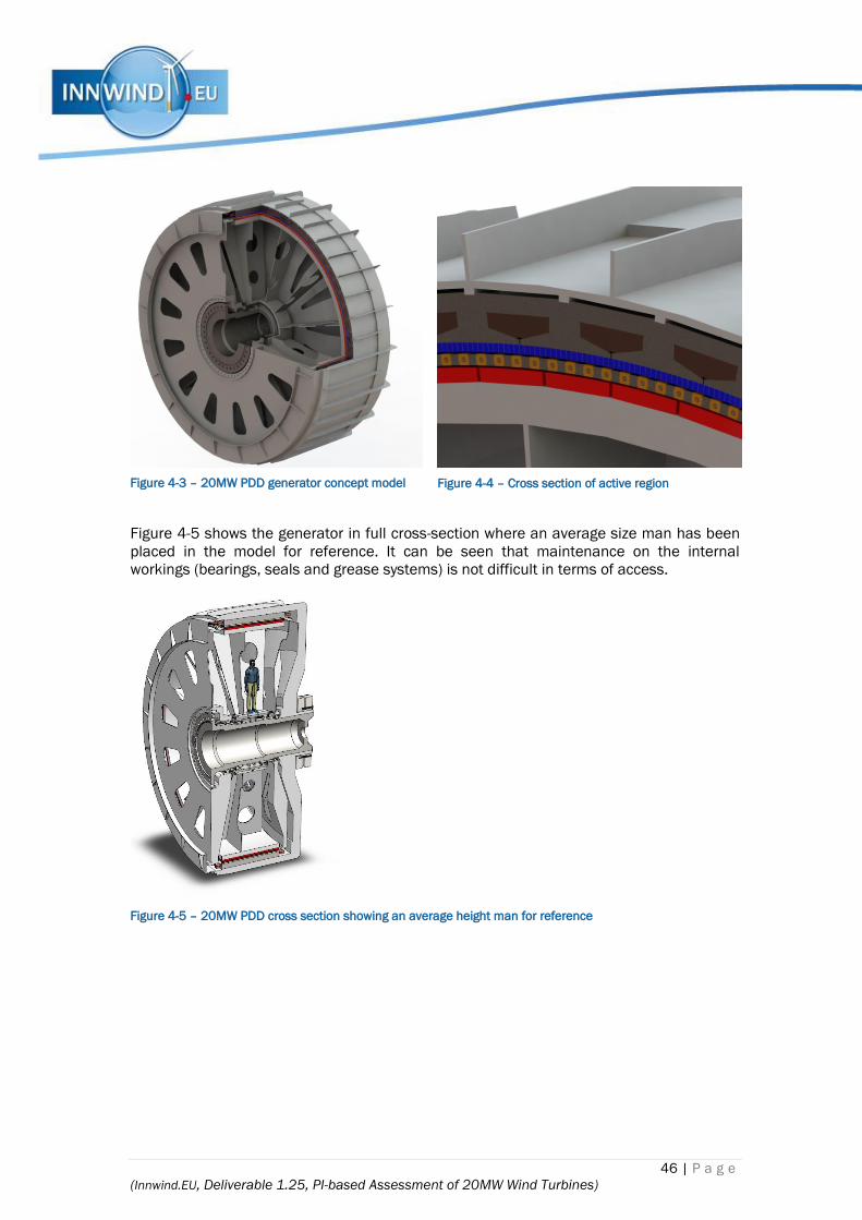
46 | P a g e
(Innwind.EU, Deliverable 1.25, PI-based Assessment of 20MW Wind Turbines)
Figure 4-3 – 20MW PDD generator concept model
Figure 4-4 – Cross section of active region
Figure 4-5 shows the generator in full cross-section where an average size man has been
placed in the model for reference. It can be seen that maintenance on the internal
workings (bearings, seals and grease systems) is not difficult in terms of access.
Figure 4-5 – 20MW PDD cross section showing an average height man for reference

47 | P a g e
(Innwind.EU, Deliverable 1.25, PI-based Assessment of 20MW Wind Turbines)
Figure 4-6 – King-pin stub-shaft and bearing details
Figure 4-7 – Active region cross section
Figure 4-8 – View of the PDD from the drive end
Figure 4-9 – Cross section showing stiffening webs
to the stator frame and rotors
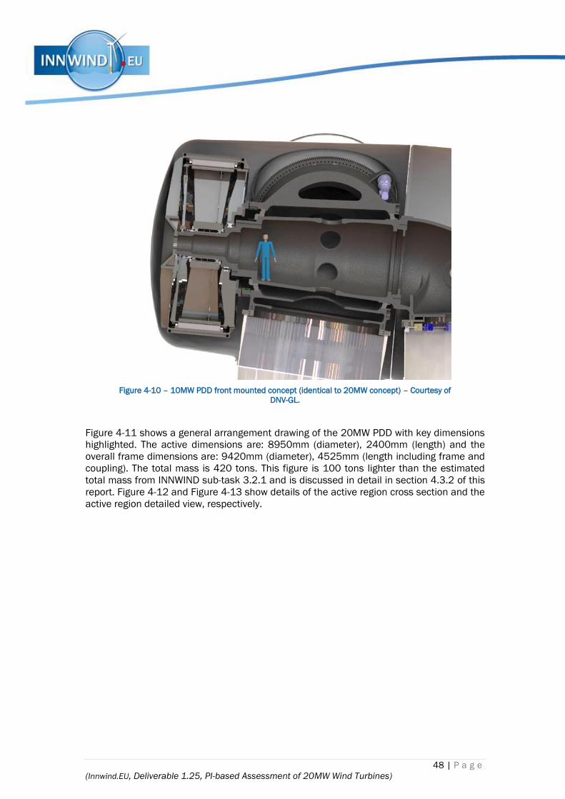
48 | P a g e
(Innwind.EU, Deliverable 1.25, PI-based Assessment of 20MW Wind Turbines)
Figure 4-10 – 10MW PDD front mounted concept (identical to 20MW concept) – Courtesy of
DNV-GL.
Figure 4-11 shows a general arrangement drawing of the 20MW PDD with key dimensions
highlighted. The active dimensions are: 8950mm (diameter), 2400mm (length) and the
overall frame dimensions are: 9420mm (diameter), 4525mm (length including frame and
coupling). The total mass is 420 tons. This figure is 100 tons lighter than the estimated
total mass from INNWIND sub-task 3.2.1 and is discussed in detail in section 4.3.2 of this
report. Figure 4-12 and Figure 4-13 show details of the active region cross section and the
active region detailed view, respectively.
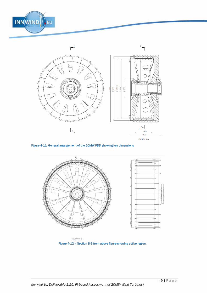
49 | P a g e
(Innwind.EU, Deliverable 1.25, PI-based Assessment of 20MW Wind Turbines)
Figure 4-11- General arrangement of the 20MW PDD showing key dimensions
Figure 4-12 – Section B-B from above figure showing active region.

50 | P a g e
(Innwind.EU, Deliverable 1.25, PI-based Assessment of 20MW Wind Turbines)
Figure 4-13 – Detail C – active region showing stator, windings, pole-piece rotor and high speed permanent
magnet rotor.
In this study, the 20MW PDD generator designed for 20 MW turbines is implemented on
an offshore steel jacket sub-structure. The 20 MW PDD design is evaluated in terms of
fatigue and ultimate loads. The resulting loads are compared to the loads obtained on the
baseline 20 MW RWT described in [1].
The 20 MW PDD turbine properties are described in Table 4-1 below and compared with
the 20 MW RWT and 10MW PDD. The PDD generator is modelled as a concentrated mass
located at 4 m upfront the rotor, whereas the nacelle weight, including other internal parts
and components, is modelled as a concentrated mass located at 8.56 m downwind the
yaw axis, acting as a counterweight. In the 20 MW RWT, the drivetrain weight is modelled
as a concentrated mass added to the nacelle weight.
Table 4-1 Comparison of the RNA parameters of the 20 MW PDD turbine with the 10 MW PDD Turbine.
10 MW PDD 20 MW PDD 20 RWT
Rotor size [m] 178 252 252
Distance along shaft from hub to Yaw axis [m] 5.31 7.13 10
Distance along shaft from hub to main bearing [m] 1.76 2.36 6.22
Hub mass [ton] 149.01 385.22 278
Hub inertia about low speed shaft [kg m^2] 2474705.87 12115772.17 1710000
Nacelle mass [ton] 240.01 587.85 1098
Nacelle inertia about Yaw axis [kg m^2] 9306677.45 45348724.05 3.607E+04
Nacelle CM downwind of yaw -5.86 -8.56 3.83
Nacelle CM above yaw 2.27 2.68 3.39
Rated rotor speed 9.60 7.14 7.14
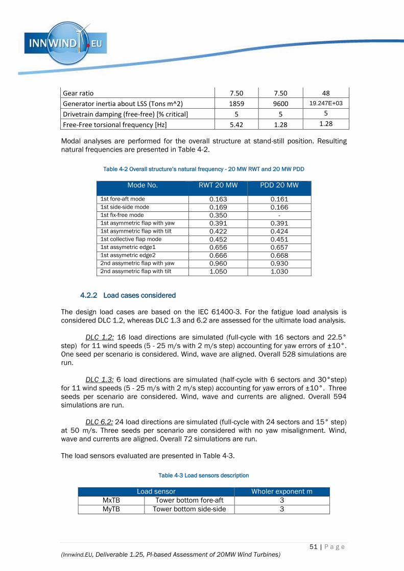
51 | P a g e
(Innwind.EU, Deliverable 1.25, PI-based Assessment of 20MW Wind Turbines)
Gear ratio 7.50 7.50 48
Generator inertia about LSS (Tons m^2) 1859 9600 19.247E+03
Drivetrain damping (free-free) [% critical] 5 5 5
Free-Free torsional frequency [Hz] 5.42 1.28 1.28
Modal analyses are performed for the overall structure at stand-still position. Resulting
natural frequencies are presented in Table 4-2.
Table 4-2 Overall structure’s natural frequency - 20 MW RWT and 20 MW PDD
Mode No. RWT 20 MW PDD 20 MW
1st fore-aft mode 0.163 0.161 1st side-side mode 0.169 0.166 1st fix-free mode 0.350 - 1st asymmetric flap with yaw 0.391 0.391 1st asymmetric flap with tilt 0.422 0.424 1st collective flap mode 0.452 0.451 1st assymetric edge1 0.656 0.657 1st assymetric edge2 0.666 0.668 2nd assymetric flap with yaw 0.960 0.930 2nd assymetric flap with tilt 1.050 1.030
4.2.2 Load cases considered
The design load cases are based on the IEC 61400-3. For the fatigue load analysis is
considered DLC 1.2, whereas DLC 1.3 and 6.2 are assessed for the ultimate load analysis.
DLC 1.2: 16 load directions are simulated (full-cycle with 16 sectors and 22.5°
step) for 11 wind speeds (5 - 25 m/s with 2 m/s step) accounting for yaw errors of ±10°.
One seed per scenario is considered. Wind, wave are aligned. Overall 528 simulations are
run.
DLC 1.3: 6 load directions are simulated (half-cycle with 6 sectors and 30°step)
for 11 wind speeds (5 - 25 m/s with 2 m/s step) accounting for yaw errors of ±10°. Three
seeds per scenario are considered. Wind, wave and currents are aligned. Overall 594
simulations are run.
DLC 6.2: 24 load directions are simulated (full-cycle with 24 sectors and 15° step)
at 50 m/s. Three seeds per scenario are considered with no yaw misalignment. Wind,
wave and currents are aligned. Overall 72 simulations are run.
The load sensors evaluated are presented in Table 4-3.
Table 4-3 Load sensors description
Load sensor Wholer exponent m
MxTB Tower bottom fore-aft 3
MyTB Tower bottom side-side 3

52 | P a g e
(Innwind.EU, Deliverable 1.25, PI-based Assessment of 20MW Wind Turbines)
MxTT Tower top tilt 3
MyTT Tower top roll 3
MzTT Tower top yaw 3
MxMB Main bearing tilt 3
MyMB Main bearing yaw 3
MzMB Main bearing torsion 3
MxBR Blade root flap 10
MyBR Blade root edge 10
MzBR Blade root torsion 10
The PDD generator is connected and supported to the main shaft using 2 main bearings
as versus one main bearing for the reference wind turbine.
4.2.3 Structural integrity verification
Ultimate load analysis is conducted for DLC1.3 and 6.2. Figure 4-14 provides an overview
of the computed ultimate loads normalized on the RWT 20 MW. It is seen a substantial
reduction of ≈50% of the shaft bending moments at the main bearing (both the upwind
and downwind bearings for PDD 20 MW) compared to the baseline model. This reduction
is partly due to the fact that there are two main bearings used now. It is also observed an
increasing MxTT–Tower Top tilt bending moment at the yaw bearing for the PDD 20 MW,
resulting in ≈40% higher loads compared to the baseline. This follows from the
overhanging additionally mass of the PDD generator located in front of the rotor at about
11.19 m from the yaw axis. For the other loads sensors evaluated in this study, a slightly
difference about 1-2% is observed between the two models for the ultimate loads. Table
4-4 summarizes the ultimate loads in terms of moments and forces for the shaft at the
main bearings, for tower top at the yaw bearing and at the interface between tower-jacket.
Figure 4-14 Comparison of ultimate loads - RWT 20 MW vs PDD 20 MW

53 | P a g e
(Innwind.EU, Deliverable 1.25, PI-based Assessment of 20MW Wind Turbines)
Table 4-4 Ultimate loads for shaft, tower top and interface - RWT 20 MW and PDD 20 MW
Shaft MxMB
[kNm]
MyMB
[kNm]
MzMB
[kNm]
FxMB
[kN]
FyMB
[kN]
FzMB
[kN]
20 MW RWT 146269 143706 45823 9914 9847 6288
20 MW PDD (UW) 75253 75446 41881 5828 5762 3200
20 MW PDD (DW) 70096 68638 6415 5821 5903 3200
Tower Top MxTT
[kNm]
MyTT
[kNm]
MzTT
[kNm]
FxTT
[kN]
FyTT
[kN]
FzTT
[kN]
20 MW RWT 131446 54095 151727 2592 5596 25103
20 MW PDD 188472 54934 153275 2795 5575 26869
Interface MxTB
[kNm]
MyTB
[kNm]
MzTB
[kNm]
FxTB
[kN]
FyTB
[kN]
FzTB
[kN]
20 MW RWT 756871 419022 153937 3370 6760 43224
20 MW PDD 706477 427643 155521 3649 6934 45013
Figure 4-15, Figure 4-16 and Figure 4-17show the mean (black), maximum (blue),
minimum (red) ultimate loads trends as function of wind speeds including DLC1.3 and
DLC6.2. A square-marker is used for the baseline model and a star-marker for the PDD
model.
Figure 4-15 Ultimate loads for MyMB – RWT 20 MW and PDD 20 MW vs wind speeds
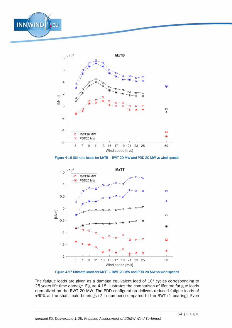
54 | P a g e
(Innwind.EU, Deliverable 1.25, PI-based Assessment of 20MW Wind Turbines)
Figure 4-16 Ultimate loads for MxTB – RWT 20 MW and PDD 20 MW vs wind speeds
Figure 4-17 Ultimate loads for MxTT – RWT 20 MW and PDD 20 MW vs wind speeds
The fatigue loads are given as a damage equivalent load of 107 cycles corresponding to
25 years life time damage. Figure 4-18 illustrates the comparison of lifetime fatigue loads
normalized on the RWT 20 MW. The PDD configuration delivers reduced fatigue loads of
≈60% at the shaft main bearings (2 in number) compared to the RWT (1 bearing). Even
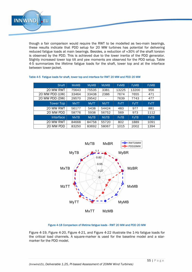
55 | P a g e
(Innwind.EU, Deliverable 1.25, PI-based Assessment of 20MW Wind Turbines)
though a fair comparison would require the RWT to be modelled as two-main bearings,
these results indicate that PDD setup for 20 MW turbines has potential for delivering
reduced fatigue loads at main bearings. Besides, a reduction of ≈30% of the shaft torsion
is observed by the PDD. This is achieved due to the lower inertia of the PDD generator.
Slightly increased tower top tilt and yaw moments are observed for the PDD setup. Table
4-5 summarizes the lifetime fatigue loads for the shaft, tower top and at the interface
between tower-jacket.
Table 4-5 Fatigue loads for shaft, tower top and interface for RWT 20 MW and PDD 20 MW
Shaft MxMB MyMB MzMB FxMB FyMB FzMB
20 MW RWT 75643 75535 3381 13225 13200 956
20 MW PDD (UW) 33464 33438 2386 7674 7655 471
20 MW PDD (DW) 29570 29542 - 7639 7743 477
Tower Top MxTT MyTT MzTT FxTT FyTT FxTT
20 MW RWT 56177 5438 54424 483 977 881
20 MW PDD 58776 5938 56752 569 973 1112
Interface MxTB MyTB MzTB FxTB FyTB FxTB
20 MW RWT 84668 84758 55720 802 1889 1091
20 MW PDD 83250 83692 58067 1015 2002 1394
Figure 4-18 Comparison of lifetime fatigue loads - RWT 20 MW and PDD 20 MW
Figure 4-19, Figure 4-20, Figure 4-21, and Figure 4-22 illustrate the 1-Hz fatigue loads for
the critical load channels. A square-marker is used for the baseline model and a star-
marker for the PDD model.

56 | P a g e
(Innwind.EU, Deliverable 1.25, PI-based Assessment of 20MW Wind Turbines)
Figure 4-19 1-Hz fatigue loads for MxTB
Figure 4-20 1-Hz fatigue loads for MyTB
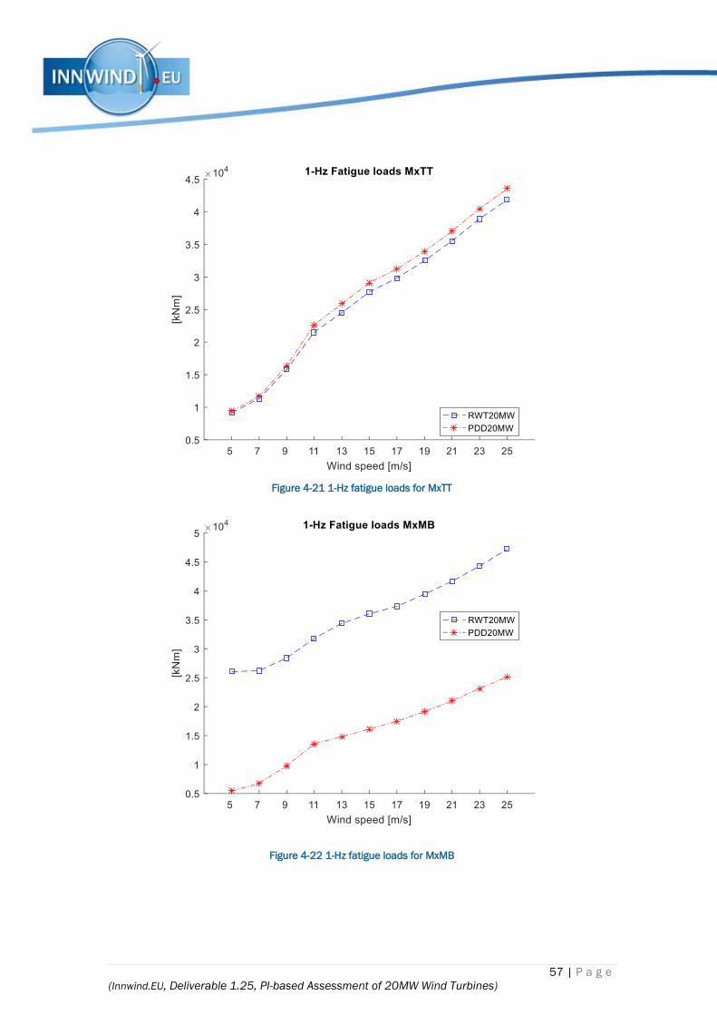
57 | P a g e
(Innwind.EU, Deliverable 1.25, PI-based Assessment of 20MW Wind Turbines)
Figure 4-21 1-Hz fatigue loads for MxTT
Figure 4-22 1-Hz fatigue loads for MxMB
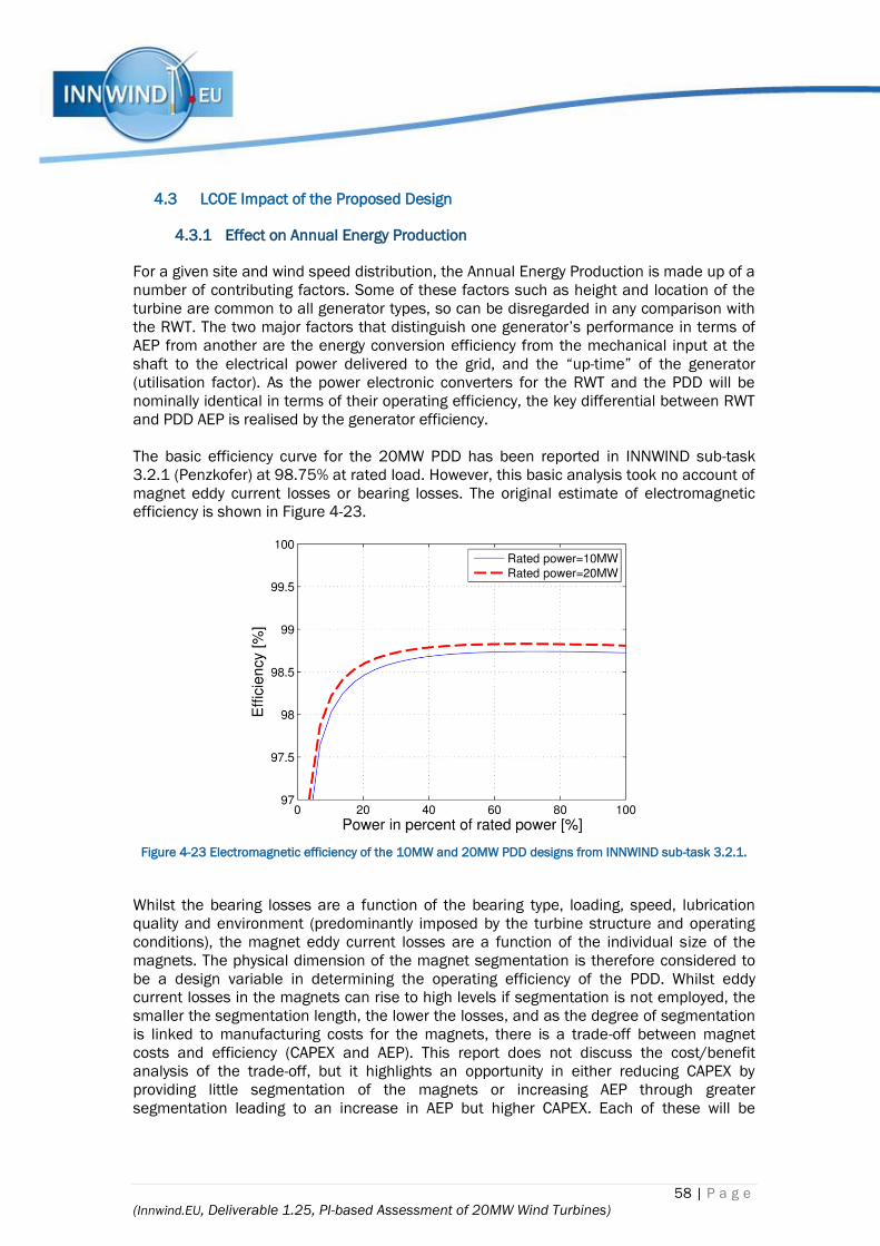
58 | P a g e
(Innwind.EU, Deliverable 1.25, PI-based Assessment of 20MW Wind Turbines)
4.3 LCOE Impact of the Proposed Design
4.3.1 Effect on Annual Energy Production
For a given site and wind speed distribution, the Annual Energy Production is made up of a
number of contributing factors. Some of these factors such as height and location of the
turbine are common to all generator types, so can be disregarded in any comparison with
the RWT. The two major factors that distinguish one generator’s performance in terms of
AEP from another are the energy conversion efficiency from the mechanical input at the
shaft to the electrical power delivered to the grid, and the “up-time” of the generator
(utilisation factor). As the power electronic converters for the RWT and the PDD will be
nominally identical in terms of their operating efficiency, the key differential between RWT
and PDD AEP is realised by the generator efficiency.
The basic efficiency curve for the 20MW PDD has been reported in INNWIND sub-task
3.2.1 (Penzkofer) at 98.75% at rated load. However, this basic analysis took no account of
magnet eddy current losses or bearing losses. The original estimate of electromagnetic
efficiency is shown in Figure 4-23.
Figure 4-23 Electromagnetic efficiency of the 10MW and 20MW PDD designs from INNWIND sub-task 3.2.1.
Whilst the bearing losses are a function of the bearing type, loading, speed, lubrication
quality and environment (predominantly imposed by the turbine structure and operating
conditions), the magnet eddy current losses are a function of the individual size of the
magnets. The physical dimension of the magnet segmentation is therefore considered to
be a design variable in determining the operating efficiency of the PDD. Whilst eddy
current losses in the magnets can rise to high levels if segmentation is not employed, the
smaller the segmentation length, the lower the losses, and as the degree of segmentation
is linked to manufacturing costs for the magnets, there is a trade-off between magnet
costs and efficiency (CAPEX and AEP). This report does not discuss the cost/benefit
analysis of the trade-off, but it highlights an opportunity in either reducing CAPEX by
providing little segmentation of the magnets or increasing AEP through greater
segmentation leading to an increase in AEP but higher CAPEX. Each of these will be

59 | P a g e
(Innwind.EU, Deliverable 1.25, PI-based Assessment of 20MW Wind Turbines)
weighted accordingly in the calculation of LCOE for offshore operation. CAPEX is discussed
in section 4.3.2 of this report.
3D analysis of eddy currents in the magnets of large PDDs has been carried out, and
segmentation lengths proposed to meet sustainable thermal management targets and
also efficiency targets. Although the magnet eddy currents have not been modelled for the
20MW concept design, it is reasonable to assume from past modelling on 300kW and
500kW generators that the efficiency will drop by around 0.25% (magnet segmentation is
carried out to such a degree to meet this condition). Hence the efficiency at rated load will
reduce from 98.75% (INNWIND sub-task 3.2.1) to 98.5% at rated load. As the magnet
eddy current losses are a function of speed squared, the shape of the efficiency curve in
Figure 4-23 would retain the same basic shape.
Overall efficiency is still higher than the RWT, where the PDD in general would allow for
about 3% increased energy capture as compared to the RWT due to the high efficiency of
energy conversion afforded by the mechanical and magnetic integration of an (effectively)
medium speed PM generator and magnetic gear. The PDD avoids the inefficiency of both a
mechanical gear system and the highly electrically stressed direct drive system.
Reliability can be a major contributor to AEP, and the subject of reliability and its effects on
OPEX is covered in section 4.3.3 of this document. It is assumed that on reaching TRL 9
for multi-megawatt size generators that a PDD generator will have the same net effect on
OPEX as a PMG due to the similar MTBFs. The effect on AEP is therefore dominated by the
increase in energy capture afforded by the PDD (~3%) which is directly proportional to a
reduction in LCOE.
A second order effect of a higher operating efficiency is the reduction in ancillary cooling
equipment requirements, which in turn acts to reduce OPEX and boost reliability.
4.3.2 Effect on CAPEX
The cost of manufacture of large PDDs has been investigated with a large generator
manufacturer and found to be close to the cost of an equivalent PMG. The comparison
included raw material costs, processing costs, tooling and manufacturing labour. The costs
for a 20MW PDD have not been considered beyond the raw material prices. In order to
gain a useful level of detail, a concept model of the 20MW PDD has been developed and a
basic bill of materials produced with all major components present, including bearings.
Table 4-6 shows the bill of materials (BOM) and mass breakdown of the 20MW PDD
generator. It can be seen that the total mass of the PDD is around 420 tons which is 100
tons lighter than the estimated mass reported in INNWIND.EU sub-task 3.2.1. The
difference is due to very basic early estimates based on simple ratios of active to
structural material, whereas the latest estimate is based on a concept solid model as
described in section 4.2.1. Table 4-7 shows the breakdown in terms of material type, the
associated material prices per ton that have been assumed in the study, the resulting
costs for each material and the total material cost of the 20MW PDD generator. It can be
seen that the total material costs are around 3.6M€.
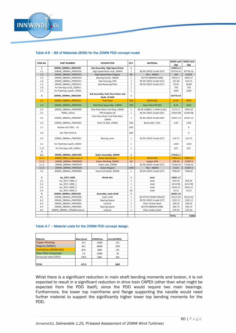
60 | P a g e
(Innwind.EU, Deliverable 1.25, PI-based Assessment of 20MW Wind Turbines)
Table 4-6 – Bill of Materials (BOM) for the 20MW PDD concept model
Table 4-7 – Material costs for the 20MW PDD concept design.
Whist there is a significant reduction in main shaft bending moments and torsion, it is not
expected to result in a significant reduction in drive train CAPEX (other than what might be
expected from the PDD itself), since the PDD would require two main bearings.
Furthermore, the tower top mainframe and flange supporting the nacelle would need
further material to support the significantly higher tower top bending moments for the
PDD.
ITEM NO. PART NUMBER DESCRIPTION QTY. MATERIALMASS each
[kg]
MASS total
[kg]
1 20MW_28MNm_SM01585 Sub-Assembly, High Speed Rotor 1 129211.6
1.1 20MW_28MNm_PM05916 High Speed Rotor Hub, 20MW 1 BS EN 10025 Grade S275 95734.16 95734.16
1.2 20MW_28MNm_PM05915 High Speed Rotor Magnet 80 Neo - N48SH 290 23200
1.3 20MW_28MNm_PM05914 Bearing Carrier, 20MW 1 BS 970 080M40 (EN8) 4924.27 4924.27
1.4 20MW_28MNm_PM05913 Seal Housing, HSR 2 BS EN 10025 Grade S275 255.06 510.12
1.5 20MW_28MNm_PM05912 Seal Retaining Plate 2 BS EN 10025 Grade S275 29.43 58.86
1.6 hsr free brg nu18_1500m1 1 750 750
1.7 hsr fixed brg nup28_1500m 1 1040 1040
2 20MW_28MNm_SM01584Sub Assembly, Pole Piece Rotor and
Shaft, 10 MW1 66776.54
2.1 20MW_28MNm_PM05911 Pole Piece 300 M450-65A 32.92 9876
2.2 20MW_28MNm_PM05910 Pole Piece Spacer Bar, 10MW 300 Glass Fibre EPC205 8.74 2622
2.3 20MW_28MNm_PM05909 Pole Piece Rotor End Ring, 10MW 2 BS EN 10088-2 1.4404 (316L) 2175.17 4350.34
2.4 PM05_20mw PPR Endplate DE 1 BS EN 10025 Grade S355 31934.98 31934.98
2.5 20MW_28MNm_PM05907Pole Piece Rotor End Plate Rear,
10MW1 BS EN 10025 Grade S355 14437.13 14437.13
2.6 20MW_28MNm_PM05902 M16 Tie Rod, 10MW 300 Bumax 88 / 316L 4.64 1392
2.7 Washer ISO 7091 - 16 600 0
2.8 ISO 7042-M16-N 600 0
2.9 20MW_28MNm_PM05901 Bearing cover 1 BS EN 10025 Grade S275 214.72 214.72
2.1 hsr fixed brg nup28_1600m 1 1320 1320
2.11 hsr free brg nu18_1400m 1 625 625
3
3.1 20MW_28MNm_SM01499 Stator Assembly, 20MW 1 176161.1
3.1.1 20MW_28Nm_stator lams 2 Stator laminations 1 M450-65A 73965.61 73965.61
3.1.2 20MW_28MNm_PM05687 Stator Winding, 20MW 60 Copper 40% 238.46 14307.6
3.1.3 20MW_28MNm_PM05675 stator case, 20MW 1 BS EN 10025 Grade S275 71346.44 71346.44
3.1.4 20MW_28MNm_PM05665 Stator Magnet 1040 Neo - N48SH 14.43 15007.2
3.2 20MW_28MNm_PM05894 Input End Shield, 20MW 1 BS EN 10025 Grade S275 7306.87 7306.87
5 tas_3071-1000 Shrink disc 1 steel 13831.17
5.1 tas_3071-1000_3 1 steel 819.34 819.34
5.2 tas_3071-1000_1 1 steel 6152.98 6152.98
5.3 tas_3071-1000_2 1 steel 6343.12 6343.12
5.4 tas_3071-1000_4 50 steel 10.31 515.5
6 20MW_28MNm_SM01583 Assembly, static Shaft 1 28201.33
6.1 20MW_28MNm_PM05906 static shaft 1 BS 970 817M40T (EN24T) 26122.62 26122.62
6.2 20MW_28MNm_PM05905 Bearing Spacer 1 BS EN 10025 Grade S275 1202.12 1202.12
6.3 20MW_28MNm_PM05904 Locknut 1 Plain Carbon Steel 330.53 330.53
6.4 20MW_28MNm_PM05903 Bearing Spacer 1 BS 970 080M40 (EN8) 269.73 269.73
6.5 20MW_28MNm_TR1600 locknut Locknut 1 Plain Carbon Steel 276.33 276.33
TOTAL 416956
Material Mass [tons] EUROS/ton Cost (kEUROS)
Copper Windings 14.3 15000 215
Magnets (N48SH) 38.2 60000 2292
Laminations (M400-65A) 83.8 3000 252
Glass Fibre Compsosite 2.6 15000 39
Structural steel (S355) 278.0 3000 834
TOTAL 417.0 3632
61 | P a g e
(Innwind.EU, Deliverable 1.25, PI-based Assessment of 20MW Wind Turbines)
4.3.3 Effect on OPEX
OPEX analysis considers all forms of expenditure to do with operations and maintenance
of the offshore turbines. Section 4.2.1 described the PDD operation and Figure 4-3 to
Figure 4-9 showed the detail of the 20MW PDD. Fundamentally, the PDD is a permanent
magnet generator with an additional rotor, so it is sensible to make comparisons with
direct drive PM generators to summarise the effect on OPEX of employing a PDD generator
in a 20MW offshore wind turbine.
The output rotor (or pole-piece rotor) is connected to the blades via a torsional coupling
(torque only connection), and the high speed rotor is free (unconnected) and rotates
internally to the output rotor. At steady state speed, there is no torque on the high speed
rotor, as this is reacted by the stator magnets. Hence, there is very little stress or strain in
the high speed rotor other than the self-loading and it is isolated from any non-torsional
loads. The high speed rotor bearings are therefore lightly loaded, and for a front-mounted
design with flexible coupling between the output rotor and blade hub, there will be
negligible influence from external sources due to wind loads. In addition, the bearings
must straddle the static output shaft in the front-mounted design which results in the
selection of over-sized bearings for the operating loads considered (~1.4m in diameter)
and thus the bearings will have a long lifetime. Magnomatics have not investigated the
lifetime of the high speed rotor bearings for such large generators, but the speeds and
loads are well within SKF bearing guidelines.
Figure 4-24 shows a cross section of the 20MW PDD where the location of the various
bearings has been highlighted. It can be seen that the two high speed bearings are
mounted on the King-pin stub-shaft. It has been assumed that the static stub shaft will be
sized to take the fatigue loads of the generator and also ensure displacement is within the
specified tolerances for the bearings so as not to reduce their life expectancy. As the front-
mounted generator is isolated to a large degree from the non-torsional loads of the blades,
this is a valid assumption.
Given that the low speed bearings (DE and NDE bearings in Figure 4-24) are common to
direct drive PMG designs, and that the high speed bearings are within established
operating loads and speeds for the given lubrication type, it is assumed that the MTBF of
the bearings can considered to be similar to that of the PMG’s. Magnomatics have no test
data to validate this assumption, and it is recommended that any follow-on programme will
include the investigation of bearing lifetimes, but if the appropriate bearing selection can
be made, then the lifetime can be similar to that of a PMG.
Rotor failure on PMGs is exceptionally rare, as much research has been poured in to
magnet containment and retaining features, corrosion prevention and magnet eddy
current loss modelling. Hence, the permanent magnet rotor can be considered to have a
similar MTBF to PMG rotors.
The pole-piece rotor of the PDD is still the subject of de-risking through various
demonstrator programmes at Magnomatics, with the latest rotor going on test in Q1 2018
at the Ocean Renewable Energy Centre in Blyth, UK. This is a 2m diameter pole-piece rotor
for a 500kW wind turbine generator that carries the same design features and employs
the same modelling as will be applied to an 8m diameter rotor for a 20MW generator.
Although at present the MTBF for a PPR at a large scale is unknown, test data from other

62 | P a g e
(Innwind.EU, Deliverable 1.25, PI-based Assessment of 20MW Wind Turbines)
smaller machines has shown that the modelling methods and manufacturing methods
result in a simple robust structure.
The stator of the PDD carries the outer magnets and details of the magnet retaining
features on a 500kW generator have been reported in INNWIND report 3.2.3. These
features ensure the magnets remain bonded in position and prevent them from entering
the airgap. A similar method has been tested on a 300kW PDD with very good results with
1000s of hours of operation without any degradation in the structure. The updated
approach that is more amenable to large machine manufacturing is currently being trialled
in the 500kW wind turbine generator under the DEMOWIND Compact High Efficiency
Generator (CHEG) project in Q1 2018 – a collaboration between Magnomatics, ATB
Laurence-Scott, ODSL and EDF.
Although the cumulative effect of all the features unique to a PDD compared to a PMG
result in the PDD being assigned a lower TRL, consideration of the current stage of
development of the PDD shows that it should be possible for a PDD to be as reliable as a
PMG after more development iterations at increasing scale have de-risked the various
novel technologies in the PPR and the magnet retaining features.
The technological differences between a PMG and a PDD should not result in increased
maintenance schedules or lower MTBF, so the effects of the potential failure modes on
OPEX can be considered to be neutral.
Figure 4-24 – Details of the king-pin stub-shaft and bearing locations.
The reduced fatigue on the main shaft due to the low inertia of the generator would allow
longer life of the main shaft and main bearings. This can in turn reduce the OPEX due to
reduction in unplanned maintenance, lower downtime and lower inventory costs.
4.4 Conclusions
A 20MW Concept design has been developed for the PDD and a detailed BOM produced
from a solid model of the generator. The capital cost of the generator has been estimated
63 | P a g e
(Innwind.EU, Deliverable 1.25, PI-based Assessment of 20MW Wind Turbines)
at 3.6M€ for materials but no further analysis was possible on manufacturing costs at this
stage.
The PDD is assumed to offer no change in OPEX compared to the RWT. The largest
contribution to a reduction in LCOE is due to the very high efficiency afforded by the
magnetic gear and electrical machine integrated combination. Rated efficiency of 98.5%
compared with the RWT drive-train results in an improved energy capture of around 3%.
The calculation of LCOE is directly proportional to the AEP to a first order, so assuming that
OPEX and CAPEX are similar, the higher energy transmission efficiency directly paves the
way for a reduction of about 3% in LCOE.
It is the responsibility of ongoing and future programs to verify the efficiency, OPEX and
CAPEX through engagement with OEMs and tier 1 suppliers on demonstrator programs
that seek to push the boundaries beyond the current largest PDD which is rated at 500kW.
Ultimate and fatigue loads analysis is evaluated for 20 MW wind turbines setup with PDD.
The 420 tons PDD is mounted upfront the rotor at a distance of 11.19 m from yaw-axis.
For a more realistic comparison with the baseline 20 MW RWT turbine, the shaft of the
PDD setup is supported by two main bearings located at respectively 2.36 m upwind and
downwind the rotor. This model configuration achieves a significant improvement over a 1
main bearing RWT in both ultimate and fatigue loads on the shaft, which suggests the PDD
as design solution for main shaft loads mitigation.
An ultimate load reduction of ≈50% has been demonstrated for the shaft bending
moments (both tilt and yaw) and a reduction of fatigue loads of ≈60%. Besides, due to
reduced inertia of the PDD generator, the fatigue torsion at the shaft is found 30% less
than baseline configuration. Eventually, due to the additional mass located upfront the
rotor in the PDD setup, increased ultimate loads of about 40% are observed for the tower-
top tilt moment compared to the baseline.

64 | P a g e
(Innwind.EU, Deliverable 1.25, PI-based Assessment of 20MW Wind Turbines)
CHAPTER 5 20MW JACKET DESIGN
The jacket design for the 20 MW wind turbine is briefly described in this chapter. The
structure has been developed using two design phases. Firstly, a jacket pre-design based
on loads of a “land version” of the 20 MW reference wind turbine [1] is developed. This
resulted in a first estimate of the overall jacket and pile geometry and dynamic properties
of the full system. Secondly, a state-of-the art load iteration procedure under due
consideration of the wind turbine and jacket and combined wind, wave loading and
structural response is considered. This approach is usually applied in detailed design
projects. An overview of the design assumptions is given and the results are summarized
in this chapter.
5.1 Introduction to the Bottom-Mounted Jacket Design
Jacket type support structures are an adequate solution for medium water depths where
monopile designs can reach manufacturing limits, dynamic limits (designs might become
too soft), installation limits or cost effective limits and on the other end floating wind
turbine concepts are mainly considered for much larger water depths. Wind farms using
jacket support structures are typically located in water depths between approximately
35 m and 60 m. The development of new load mitigation concepts opens up the
opportunity to realize monopiles also for increasing water depths. Hence the lower limit of
the water depth for jackets will probably increase. However, the jacket concept is chosen
as it is usually a robust design and geometry changes of the jacket have minor influences
on the performance of the wind turbine components. Therefore optimization of the wind
turbine rotor and drive train is possible considering only a pre-design of the jacket.
The main elevations and measures relevant for the jacket design considering the 20 MW
reference wind turbine are outlined in Figure 5-1 in comparison to the 10 MW design. It
should be noted that the assumption within the project consortium was to maintain the
water depth and interface elevation (tower to transition piece interface) and also to apply a
rather long offshore tower (extended by 12m) in order to achieve a relatively soft design
that avoids unfavorable 3p excitations from the wind turbine, which was the case for the
10 MW jacket design. The resulting minimum distance between interface elevation and
lowest blade tip elevation is therefore approximately 16 m for this 20 MW wind turbine
configuration.
From the perspective of the foundation designer a much shorter offshore tower and
somewhat higher TP would be recommended. This would improve the load transfer into
the jacket and reduces bending moments on the support structure. Of course one has to
evaluate if other requirements are contrary to this and does not allow the proposed
modifications. A shorter tower will also influence the annual energy production because of
the lower mean wind speed at a lower hub height. For example the mean wind speed at
hub height is reduced by 0.4% assuming a wind profile exponent alpha of 0.12 and a
reduction of 5 m of hub height.
The load analysis of the land version of the 20 MW reference wind turbine [1] considers
three different onshore towers, called “Tower 1” to “Tower 3”. They differ in the cross
sections and material properties but have the same tower length of 163.14 m. The towers
have different overall stiffness and thus the first natural frequency varies between
0.184 Hz and 0.208 Hz. For these three configurations the calculated wind loads time
series are generated and can be used for the jacket pre-design. The loads are given at the
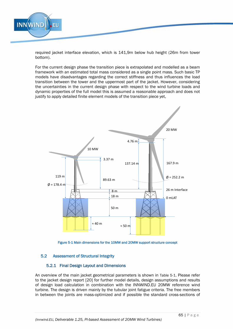
65 | P a g e
(Innwind.EU, Deliverable 1.25, PI-based Assessment of 20MW Wind Turbines)
required jacket interface elevation, which is 141,9m below hub height (26m from tower
bottom).
For the current design phase the transition piece is extrapolated and modelled as a beam
framework with an estimated total mass considered as a single point mass. Such basic TP
models have disadvantages regarding the correct stiffness and thus influences the load
transition between the tower and the uppermost part of the jacket. However, considering
the uncertainties in the current design phase with respect to the wind turbine loads and
dynamic properties of the full model this is assumed a reasonable approach and does not
justify to apply detailed finite element models of the transition piece yet,
Figure 5-1 Main dimensions for the 10MW and 20MW support structure concept
5.2 Assessment of Structural Integrity
5.2.1 Final Design Layout and Dimensions
An overview of the main jacket geometrical parameters is shown in Table 5-1. Please refer
to the jacket design report [20] for further model details, design assumptions and results
of design load calculation in combination with the INNWIND.EU 20MW reference wind
turbine. The design is driven mainly by the tubular joint fatigue criteria. The free members
in between the joints are mass-optimized and if possible the standard cross-sections of
89.63 m
18 m
50 m
3.37 m
8 m
119 m
167.9 m
0 mLAT
26 m Interface
4.76 m
137.14 m
Ø = 252.2 m
Ø = 178.4 m
≈ 40 m≈ 50 m
10 MW
20 MW

66 | P a g e
(Innwind.EU, Deliverable 1.25, PI-based Assessment of 20MW Wind Turbines)
manufactures are considered. Typically steps in ¼ of inches are applied for wall
thicknesses and full inches for diameters. The long members between two joints are
discretized in four sub-elements. All members and details such as free tubular members,
joints, circumferential single-sided and double-sided butt welds and attachment welds, are
individual checked regarding excessive yielding and buckling in ULS with appropriate
safety margins for loads and materials and regarding the achieved lifetime in FLS with a
damage fatigue factor of 3.0. The design is based on the design guideline DNVGL-ST-
0126.
The diameters and wall thicknesses of the offshore tower are taken from the scaled
onshore tower model, but the length is shortened from the bottom to comply with the
elevations given in Figure 5-1. Therefore the lower end of the onshore tower is cut at 26 m
where it has a diameter of 11.1m. The total mass of the resulting offshore tower is
approximately 1356 tons. The first natural frequency of the offshore model assuming a
rigid support at tower bottom is approximately 0.3 Hz, which is significantly higher than the
full model natural frequency including jacket and soil flexibility, see Table 5-1.
Table 5-1 Overview of jacket geometry and masses
Structural member Dimensions Value
Jacket
Base Width [m] 38
Top Width [m] 20
Interface elevation [m] wrt MSL 26
Transition Piece height [m] 4*
Number of legs [-] 4
Jacket legs diameter (outer) [mm] 1829-2642
Jacket legs maximum wall thickness [mm] 101.6
Jacket legs minimum wall thickness [mm] 44.5
Number of x-braces levels [-] 4
Diameter upper x-braces diameters (outer) [mm] 914
Diameter middle upper x-braces diameters (outer) [mm] 965 / 1219
Diameter middle lower x-braces diameters (outer) [mm] 965 / 1219
Diameter lower x-braces diameters (outer) [mm] 1168 / 1828
Braces wall thicknesses [mm] 20 - 40.5
Number of Piles [-] 4
Pile penetration [m] 50
Pile diameter [mm] 3500
Pile wall thicknesses [mm] 34.9 – 73
Pile top elevation above mudline (Stick-up length) [m] 1.8
Overlap length (grout length) [m] 7.5
Mass
Jacket structure [t] 1670
Transition Piece (estimation) [t] 450
Steel Appurtenances (estimation) [t] 50
Piles [t] 4x 230
Total lifting mass (no piles) [t] 2170
Natural frequency overall structure
1st eigenfrequency (1st bending mode) [Hz] 0.165

67 | P a g e
(Innwind.EU, Deliverable 1.25, PI-based Assessment of 20MW Wind Turbines)
5.2.2 Design Load Cases and Load Calculation Method
The load calculations are based on IEC 61400-3 design load cases (DLC) with appropriate
partial safety factors. It is assumed that the turbine has 100% technical availability, which
is a conservative assumption because the jacket design is driven by operational wind
loads and not from idling load cases. Wind and waves are aligned and 12 directions (30°
increment) are considered. Turbulent seeds are combined with a yaw error of ±8 degree.
The following DLCs have been applied:
DLC 1.2 FLS (normal operation)
DLC 6.4 FLS (idling operation)
DLC 6.2 ULS (50 year extreme wind and wave conditions)
Serviceability limit state (SLS) is not considered in the present design level. The wind
turbine manufacturer normally prescribes an allowable permeant rotation (tilt) of the
structure against the horizontal plane. It is a combination of installation tolerance and
settlement during service lifetime and has to be checked accordingly in a detailed design
assessment. The 20 MW INNWIND.EU reference wind turbine does not prescribe allowable
tilt angles. Furthermore such requirement is not a design driver for the primary steel of the
jacket, but influences usually the required minimum pile penetration length.
The pre-design phase is carried out using the results of the onshore wind turbine model,
thus a superposition approach of the loads is considered. In this approach the wind load
time series (Fx…Mz) at interface elevation from the wind-only analysis are applied to the
jacket and are combined with the wave loads from random sea states using airy wave
theory and the JONSWAP spectrum. The considered significant wave heights and wave
periods correlate with the mean wind speed. However, the dynamic interaction of loads
and support structure response cannot be considered accurately in this approach.
Furthermore all models from the wind-only analysis have a higher first natural frequency
than the full offshore model including the jacket. Therefore it must be assumed that the
wind loads and generally the load spectra will change in subsequent design iterations and
requires also an update of the 20 MW wind turbine model and controller parameters to
generally improve the design.
The conceptual design phase considers a sequential integrated simulation approach. A
super-element approximation of the jacket and correlating wave loads has been calculated
and both are implemented in the 20 MW reference wind turbine model in order to
calculate the full system response of the offshore configuration shown in Figure 5-1. The
resulting interface loads at tower bottom are subsequently applied in the design
assessment of the detailed jacket together with the local wave loads to determine the
local stresses in the jacket structure more accurately. However, an improved model of the
20 MW wind turbine, tower and controller is not developed in the project and thus it can
be assumed that the results for the jacket are conservative.
5.2.3 Structural Integrity Check
Design assessment regarding NFA, ULS and FLS for the jacket is based on the DNV
guideline, ref. [21] and [22]. Appropriate safety factors for loads and material are taken

68 | P a g e
(Innwind.EU, Deliverable 1.25, PI-based Assessment of 20MW Wind Turbines)
into account. No tower design has been carried out. The given tower geometry is based
solely on upscaling.
The purpose of the NFA analysis is to determine the natural frequency of the entire
structure or the range of frequencies to be expected from varying design assumptions. The
first natural frequency should be outside the 1P and 3P bandwidth of the wind turbine to
avoid unfavorable resonance excitations. The 1P excitation corresponds to the rotor speed
range and the 3P excitation corresponds to the blade passing frequency, which is three
times the rotor speed range.
Figure 5-2 Operational and 1st jacket natural frequencies
However, the allowed soft-stiff range of the slow rotating 20 MW reference wind turbine is
very small (0.11 - 0.12 Hz) and in practice it will not be possible to design the support
structure for this range (see Figure 5-2). It will also not be possible to reach the stiff-stiff
design which requires a natural frequency above 0.35 Hz or a soft-soft design which
requires a frequency below 0.04 Hz. Furthermore, such low frequencies are within the
wave periods and it would be reasonable to aim for higher natural frequencies if possible.
Finally this means that it cannot be fully avoided that the target frequency of the support
structure will result in a 3p excitation, which requires an appropriate controller strategy.
Resonance problems can hardly be avoided and ideally they occur at rotor speeds with low
wind speed, thus lower aerodynamic loads.
69 | P a g e
(Innwind.EU, Deliverable 1.25, PI-based Assessment of 20MW Wind Turbines)
The obtained natural frequency of the system will be utilized in other analyses, such as the
fatigue analysis, where the damping of the system is calculated by applying Rayleigh-
damping.
The purpose of the extreme event analysis is to ensure that the jacket structure and piles
are capable of supporting the WTG for the least favorable combination of environmental
load conditions. The element stresses and tubular joints punching shear stresses are
analyses for all members and load cases. The maximum allowed utilization has to be
smaller than 1.0. The governing pile design loads are also calculated in ULS, which
subsequently determines the minimum required pile penetration found in the geotechnical
analysis. ULS criteria are fulfilled for the pre-design phase and the conceptual design
phase.
The purpose of the time domain fatigue analysis is to ensure that the jacket structure is
capable of supporting the WTG for the required design life of 25 years. In addition, site
specific conditions in terms of water depth, marine growth, corrosion allowance and soil
characteristics are applied for the turbine location. Hot spot stresses are calculated using
the approach of stress concentration factors (SCF) and evaluated using a Rainflow
counting method. S-N curves for different types of tubular joint welds, butt welds, cut-outs,
conical sections and attachment welds are considered. The annual damage is calculated
using the probabilities of every time series. The resulting fatigue lifetime is equal to the
inverse of the annual damage. The results from the pre-design phase show sufficient
lifetime throughout the jacket, but requires also post-weld treatment at a number of
critical joints.
The conceptual design phase using integrated offshore load analyses show substantially
different fatigue results. The lower part of the jacket (legs and braces) is prone to local
bending vibrations, which cause high fatigue damage. Until the end of the work no final
solution has been found since only the jacket geometry was modified without
improvements of the wind turbine model or controller. Hence, a number of fatigue still
details have insufficient lifetime and it is believed not realistic to develop a jacket design
by increasing simply wall thicknesses or member diameters currently. It clearly shows the
need for closer collaborations between wind turbine designer and foundation designer to
solve these problems.
5.3 LCOE Impact
5.3.1 Effect on Annual Energy Production
The influence of the jacket, i.e. the motion of the structure, on the annual energy
production of the wind turbine is negligible. The gained power is mainly driven by the mean
wind speed and probability distribution of wind speeds, the rotor performance and the
availability of the turbine.
5.3.2 Effect on CAPEX
Costs drivers for the support structure are the material costs (raw mass of the structure),
the welding costs (number of welds and volume/length), the assembly costs and hourly
rates for equipment and workers. Due to the complexity of such cost models and the
volatile cost assumptions in the market it is more appropriate to consider lumped prices
per tonnage of the structure. The lumped prices are defined for pile steel, jacket steel and
70 | P a g e
(Innwind.EU, Deliverable 1.25, PI-based Assessment of 20MW Wind Turbines)
TP steel individually and thus expresses other cost shares through the specific mass of the
component. Furthermore such lumped price cost models are sufficiently accurate when
considering the present design maturity of the 20 MW offshore wind turbine in general. It
should be noted that the 20MW reference wind turbine is up-scaled from the 10MW class
(and also from the 5MW class) it is believed that the governing design loads are not
realistic and probably too conservative.
5.3.3 Effect on OPEX
There are no OPEX related cost savings. The support structure is designed to survive the
entire lifetime without maintenance of the primary steel components. However, it can be
assumed that inspection services are required to validate the jacket design assumptions
regarding corrosion allowance and scour development. Due to the larger dimensions of the
structure the time needed for such work could be longer und thus result in higher OPEX
costs. Precise OPEX cost estimates have not been estimated and generally contribute less
to the overall project costs.
5.4 LCOE Sensitivity Analyses
A LCOE variation study using the INNWIND.EU cost model (v1.02.1 of May 2016) of the
20 MW reference wind turbine is performed. The influence of the CAPEX costs of the
support structure on the LCOE is addressed. The LCOE calculation neglects variations of
the installation costs because the structural optimization of the support structure will
primarily influence member diameters, wall thicknesses and masses but will not end up in
a substantial change of the general proportions. Thus the installation equipment and
vessels will be unchanged. An impact on the installation time can be more relevant in
cases where the optimization results in shorter pile penetration and thus can results in
faster installation of the pre-installed piles. The results of the CAPEX variation study are
shown in Table 5-2:
Table 5-2 LCOE variation study for bottom fixed support structure costs
Support structure cost LCOE Change of LCOE
Ref. jacket design
(TP, Jacket, Piles)
13.940 mio € 93.22 €/MWh -
Jacket +10% 15.340 mio € 94.56 €/MWh +1.44%
Jacket +5% 14.640 mio € 93.89 €/MWh +0.72%
Jacket -5% 13.250 mio € 92.55 €/MWh -0.72%
Jacket -10% 12.550 mio € 91.88 €/MWh -1.44%
Jacket -20% 11.150 mio € 90.53 €/MWh -2.89%
5.5 Conclusions
A pre-design of a 20MW jacket support structure with pre-installed piles has been
successfully developed. The design is based on NFA, ULS and FLS assessments and
clearly the fatigue requirements are most critical for the design. The natural frequencies of
the whole structure are lower as initially anticipated in the load calculation of the 20 MW
reference wind turbine. Therefore, it is not surprising that the differences between the pre-
design loads (onshore loads) and the conceptual loads (integrated loads) are significant.

71 | P a g e
(Innwind.EU, Deliverable 1.25, PI-based Assessment of 20MW Wind Turbines)
Considering the fatigue results of the conceptual design it is believed very important to
optimize the jacket including optimization of the wind turbine at the same time. Thus,
stronger collaboration between wind turbine designer and foundation designer is required.
The interaction between loads and response of the structure is significant for these large
wind turbines. Traditional soft-stiff support structure designs are not feasible due to the
narrow allowed range between 1p and 3p rotor frequencies of the very slow rotating rotor.
The final FLS analysis show insufficient lifetimes and requires further design iterations
including improvements of the wind turbine performance.
The foundation costs influence only the CAPEX of the wind turbine system there is no
benefit for the energy yield. There is also no influence on operational costs in the scope of
the primary steal design.
72 | P a g e
(Innwind.EU, Deliverable 1.25, PI-based Assessment of 20MW Wind Turbines)
CHAPTER 6 ADVANCED CONTROL OF 20MW RWT
In this chapter, we describe the control methodologies applied to the variations of the
INNWIND 20 MW wind turbine. The methodologies applied are a combination of mature
advanced control methods (TRL 9) and control methods using novel sensors and actuators
(TRL ≤6). The controllers are designed to maintain wind turbine power capture levels whilst
alleviating fatigue and extreme loading on the wind turbine. We show the pathways to load
reduction for each method.
LCOE reduction facilitated by control design is most effective when combined in an
iterative design procedure with all turbine components. Therefore, the design loads
produced are not a complete indication of the load reduction potential of applying
advanced control.
6.1 Introduction to the Innovative Concept
The innovative concepts presented here are explained in further detail in controller
focused INNWIND.EU deliverables 1.43 and 1.44. The goal of each control feature is to
reduce turbine loading. The loading margin can then be used in to reduce overall LCOE
through:
Increasing rotor size for larger AEP;
Increasing capacity factor by increasing the operational conditions of the turbine
(wind speed, turbulence intensity and sea state).
Reducing loading requirements of turbine components
6.1.1 In-plane damping (TRL 9 – Essential)
The INNWIND 20 MW RWT shows very low damping (<2%) of the first collective in-plane
mode of the turbine at 1.27 Hz. This coupled mode includes effects from the first and
second blade edgewise collective mode, the 2nd and 3rd tower side-side modes. These
modes are also at risk from destabilisation under closed-loop speed control. Therefore, in-
plane damping is required to keep drivetrain in-plane loading at feasible levels.
Traditionally the low-speed shaft (LSS) flexibility was the key determinant of the first in-
plane frequency and showed the least damping; however, for the 20 MW RWT the
drivetrain flexibility has a frequency of 3.65 Hz which is typically outside the bandwidth of
any control loop and shows a reasonable damping level of 4.3%. Figure 6-1 and Figure 6-2
show the linear frequency response and step responses of the damped and un-damped
systems at 12 m/s respectively. Note that damping has increased the response of the LSS
around 2 Hz, though the energy content of the wind at 2 Hz is much less than at 1.27 Hz,
so there is a net benefit in fatigue damage reduction. The damper takes the form of a
bandpass filter from generator speed measurements to generator torque demand; an
example frequency response of the filter is shown in Figure 6-3.
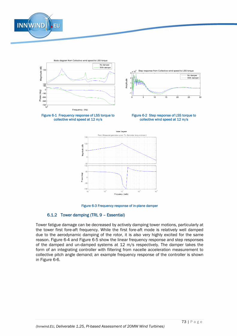
73 | P a g e
(Innwind.EU, Deliverable 1.25, PI-based Assessment of 20MW Wind Turbines)
Figure 6-1 Frequency response of LSS torque to
collective wind speed at 12 m/s
Figure 6-2 Step response of LSS torque to
collective wind speed at 12 m/s
Figure 6-3 Frequency response of in-plane damper
6.1.2 Tower damping (TRL 9 – Essential)
Tower fatigue damage can be decreased by actively damping tower motions, particularly at
the tower first fore-aft frequency. While the first fore-aft mode is relatively well damped
due to the aerodynamic damping of the rotor, it is also very highly excited for the same
reason. Figure 6-4 and Figure 6-5 show the linear frequency response and step responses
of the damped and un-damped systems at 12 m/s respectively. The damper takes the
form of an integrating controller with filtering from nacelle acceleration measurement to
collective pitch angle demand; an example frequency response of the controller is shown
in Figure 6-6.
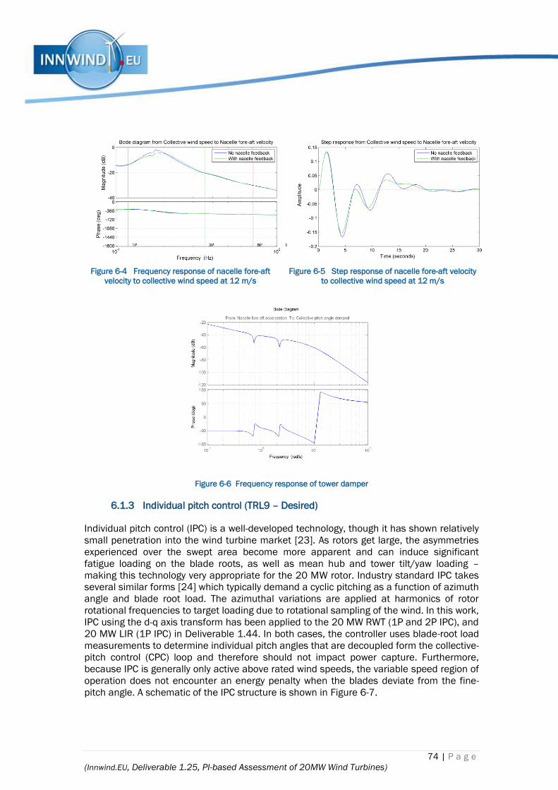
74 | P a g e
(Innwind.EU, Deliverable 1.25, PI-based Assessment of 20MW Wind Turbines)
Figure 6-4 Frequency response of nacelle fore-aft
velocity to collective wind speed at 12 m/s
Figure 6-5 Step response of nacelle fore-aft velocity
to collective wind speed at 12 m/s
Figure 6-6 Frequency response of tower damper
6.1.3 Individual pitch control (TRL9 – Desired)
Individual pitch control (IPC) is a well-developed technology, though it has shown relatively
small penetration into the wind turbine market [23]. As rotors get large, the asymmetries
experienced over the swept area become more apparent and can induce significant
fatigue loading on the blade roots, as well as mean hub and tower tilt/yaw loading –
making this technology very appropriate for the 20 MW rotor. Industry standard IPC takes
several similar forms [24] which typically demand a cyclic pitching as a function of azimuth
angle and blade root load. The azimuthal variations are applied at harmonics of rotor
rotational frequencies to target loading due to rotational sampling of the wind. In this work,
IPC using the d-q axis transform has been applied to the 20 MW RWT (1P and 2P IPC), and
20 MW LIR (1P IPC) in Deliverable 1.44. In both cases, the controller uses blade-root load
measurements to determine individual pitch angles that are decoupled form the collective-
pitch control (CPC) loop and therefore should not impact power capture. Furthermore,
because IPC is generally only active above rated wind speeds, the variable speed region of
operation does not encounter an energy penalty when the blades deviate from the fine-
pitch angle. A schematic of the IPC structure is shown in Figure 6-7.
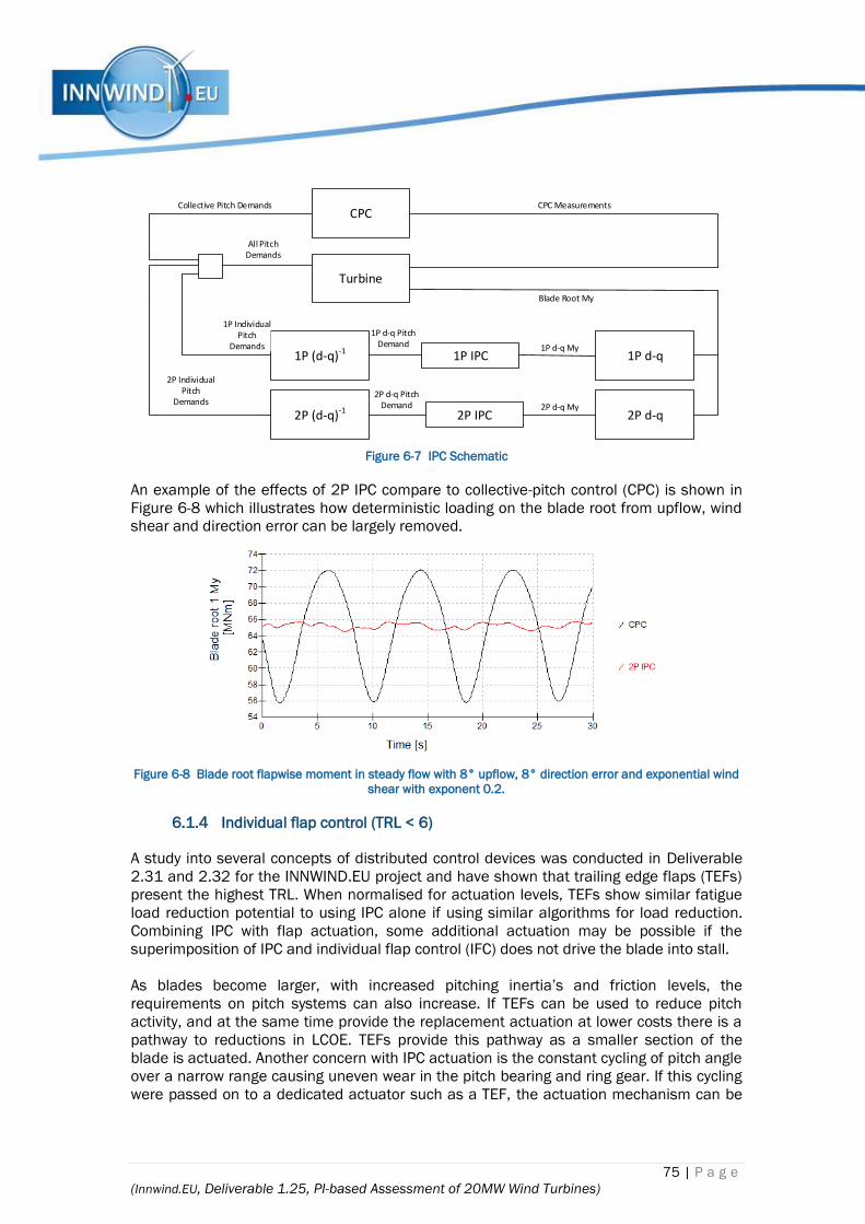
75 | P a g e
(Innwind.EU, Deliverable 1.25, PI-based Assessment of 20MW Wind Turbines)
Turbine
CPC
1P IPC
2P IPC
1P d-q
2P d-q
1P (d-q)-1
2P (d-q)-1
CPC MeasurementsCollective Pitch Demands
All PitchDemands
1P Individual Pitch
Demands
2P IndividualPitch
Demands
Blade Root My
1P d-q Pitch Demand
2P d-q Pitch Demand
1P d-q My
2P d-q My
Figure 6-7 IPC Schematic
An example of the effects of 2P IPC compare to collective-pitch control (CPC) is shown in
Figure 6-8 which illustrates how deterministic loading on the blade root from upflow, wind
shear and direction error can be largely removed.
Figure 6-8 Blade root flapwise moment in steady flow with 8° upflow, 8° direction error and exponential wind
shear with exponent 0.2.
6.1.4 Individual flap control (TRL < 6)
A study into several concepts of distributed control devices was conducted in Deliverable
2.31 and 2.32 for the INNWIND.EU project and have shown that trailing edge flaps (TEFs)
present the highest TRL. When normalised for actuation levels, TEFs show similar fatigue
load reduction potential to using IPC alone if using similar algorithms for load reduction.
Combining IPC with flap actuation, some additional actuation may be possible if the
superimposition of IPC and individual flap control (IFC) does not drive the blade into stall.
As blades become larger, with increased pitching inertia’s and friction levels, the
requirements on pitch systems can also increase. If TEFs can be used to reduce pitch
activity, and at the same time provide the replacement actuation at lower costs there is a
pathway to reductions in LCOE. TEFs provide this pathway as a smaller section of the
blade is actuated. Another concern with IPC actuation is the constant cycling of pitch angle
over a narrow range causing uneven wear in the pitch bearing and ring gear. If this cycling
were passed on to a dedicated actuator such as a TEF, the actuation mechanism can be
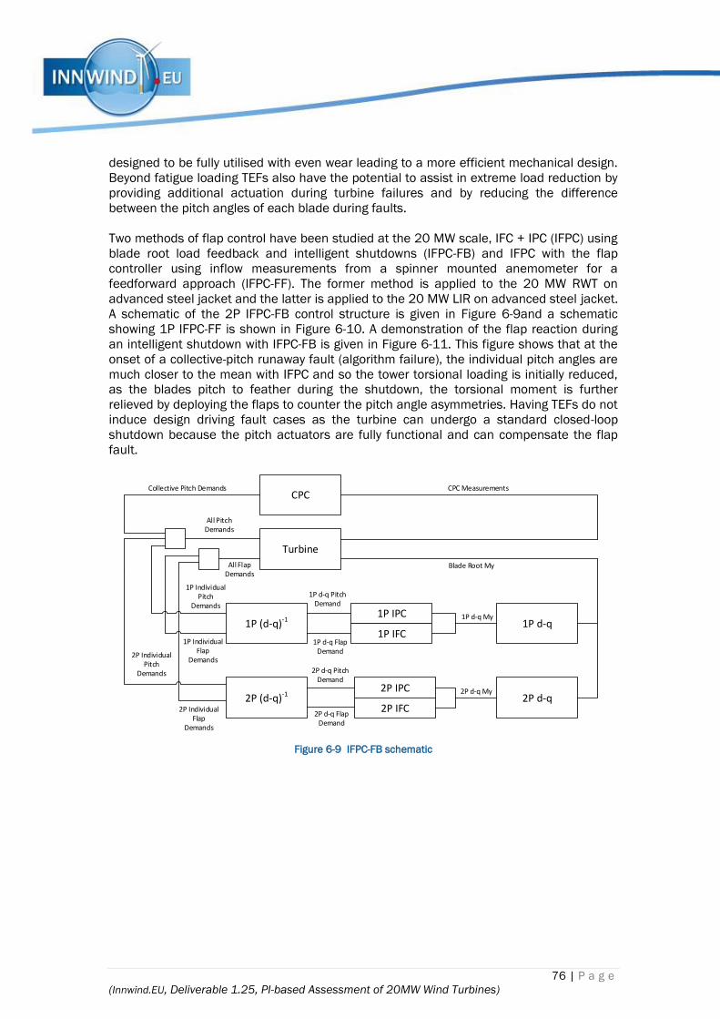
76 | P a g e
(Innwind.EU, Deliverable 1.25, PI-based Assessment of 20MW Wind Turbines)
designed to be fully utilised with even wear leading to a more efficient mechanical design.
Beyond fatigue loading TEFs also have the potential to assist in extreme load reduction by
providing additional actuation during turbine failures and by reducing the difference
between the pitch angles of each blade during faults.
Two methods of flap control have been studied at the 20 MW scale, IFC + IPC (IFPC) using
blade root load feedback and intelligent shutdowns (IFPC-FB) and IFPC with the flap
controller using inflow measurements from a spinner mounted anemometer for a
feedforward approach (IFPC-FF). The former method is applied to the 20 MW RWT on
advanced steel jacket and the latter is applied to the 20 MW LIR on advanced steel jacket.
A schematic of the 2P IFPC-FB control structure is given in Figure 6-9and a schematic
showing 1P IFPC-FF is shown in Figure 6-10. A demonstration of the flap reaction during
an intelligent shutdown with IFPC-FB is given in Figure 6-11. This figure shows that at the
onset of a collective-pitch runaway fault (algorithm failure), the individual pitch angles are
much closer to the mean with IFPC and so the tower torsional loading is initially reduced,
as the blades pitch to feather during the shutdown, the torsional moment is further
relieved by deploying the flaps to counter the pitch angle asymmetries. Having TEFs do not
induce design driving fault cases as the turbine can undergo a standard closed-loop
shutdown because the pitch actuators are fully functional and can compensate the flap
fault.
Turbine
CPC
1P IPC
1P IFC
2P IPC
2P IFC
1P d-q
2P d-q
1P (d-q)-1
2P (d-q)-1
CPC MeasurementsCollective Pitch Demands
All PitchDemands
All FlapDemands
1P Individual Pitch
Demands
2P IndividualPitch
Demands
1P IndividualFlap
Demands
2P IndividualFlap
Demands
Blade Root My
1P d-q Pitch Demand
2P d-q Pitch Demand
1P d-q FlapDemand
2P d-q Flap Demand
1P d-q My
2P d-q My
Figure 6-9 IFPC-FB schematic

77 | P a g e
(Innwind.EU, Deliverable 1.25, PI-based Assessment of 20MW Wind Turbines)
Figure 6-10 IFPC-FF schematic
Figure 6-11 Time series response of DLC 2.2 eb2 (Collective pitch runaway) inder IPC and IFPC-FB
6.1.5 Extreme turbulence control (TRL < 6)
A new control strategy is proposed for reduction of extreme loads on wind turbine
components during operation in extreme turbulence conditions, such as those specified in
θyaw
θtilt
t
1P
t
Instantaneous
filtered θyaw
Instantaneous
filtered θtilt
Instantaneous
filtered U
Predefined
Lookup
Table
yaw tilt 1 1
2 2
(U, , , ) cos( )
cos(2 )
flap f
f
1 2 yaw tilt
1 2 yaw tilt
, (U, , )
, (U, , )
f f
t
flap
flapMno control
spinner control
1P
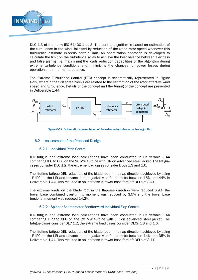
78 | P a g e
(Innwind.EU, Deliverable 1.25, PI-based Assessment of 20MW Wind Turbines)
DLC 1.3 of the norm IEC 61400-1 ed.3. The control algorithm is based on estimation of
the turbulence in the wind, followed by reduction of the rated rotor speed whenever this
turbulence estimate exceeds certain limit. An optimization approach is developed to
calculate the limit on the turbulence so as to achieve the best balance between alertness
and false alarms, i.e. maximizing the loads reduction capabilities of the algorithm during
extreme turbulence conditions and minimizing the chances for power losses during
operation under normal turbulence.
The Extreme Turbulence Control (ETC) concept is schematically represented in Figure
6-12, wherein the first three blocks are related to the estimation of the rotor-effective wind
speed and turbulence. Details of the concept and the tuning of the concept are presented
in Deliverable 1.44.
Figure 6-12 Schematic representation of the extreme turbulence control algorithm
6.2 Assessment of the Proposed Design
6.2.1 Individual Pitch Control
IEC fatigue and extreme load calculations have been conducted in Deliverable 1.44
comparing IPC to CPC on the 20 MW turbine with LIR on advanced steel jacket. The fatigue
cases consider DLC 1.2, the extreme load cases consider DLCs 1.3 and 1.6.
The lifetime fatigue DEL reduction, of the blade root in the flap direction, achieved by using
1P IPC on the LIR and advanced steel jacket was found to be between 15% and 44% in
Deliverable 1.44. This resulted in an increase in tower base fore-aft DELs of 3-4%.
The extreme loads on the blade root in the flapwise direction were reduced 6.9%, the
tower base combined overturning moment was reduced by 3.5% and the tower base
torsional moment was reduced 14.2%.
6.2.2 Spinner Anemometer Feedforward Individual Flap Control
IEC fatigue and extreme load calculations have been conducted in Deliverable 1.44
comparing IFPC to CPC on the 20 MW turbine with LIR on advanced steel jacket. The
fatigue cases consider DLC 1.2, the extreme load cases consider DLCs 1.3 and 1.6.
The lifetime fatigue DEL reduction, of the blade root in the flap direction, achieved by using
1P IPC on the LIR and advanced steel jacket was found to be between 14% and 35% in
Deliverable 1.44. This resulted in an increase in tower base fore-aft DELs of 3-7%.
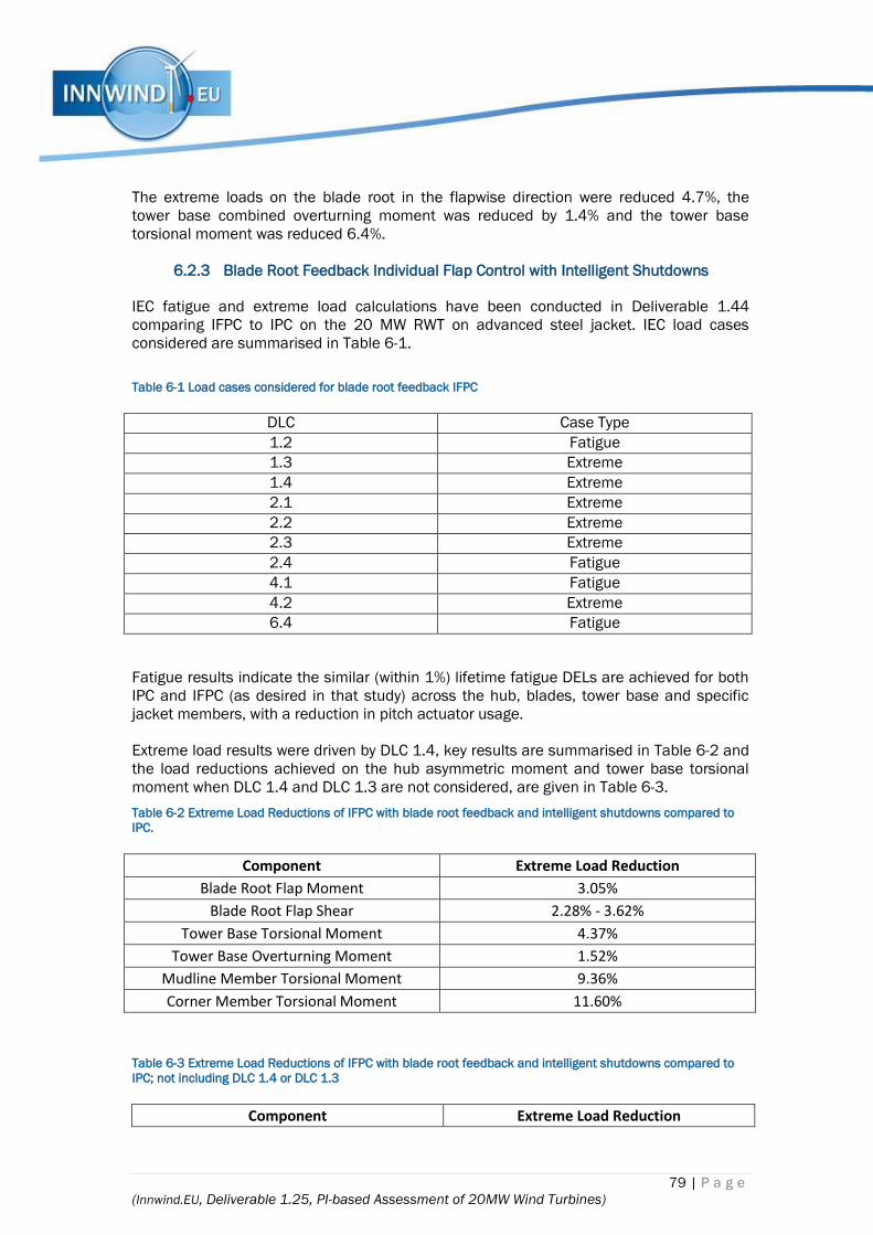
79 | P a g e
(Innwind.EU, Deliverable 1.25, PI-based Assessment of 20MW Wind Turbines)
The extreme loads on the blade root in the flapwise direction were reduced 4.7%, the
tower base combined overturning moment was reduced by 1.4% and the tower base
torsional moment was reduced 6.4%.
6.2.3 Blade Root Feedback Individual Flap Control with Intelligent Shutdowns
IEC fatigue and extreme load calculations have been conducted in Deliverable 1.44
comparing IFPC to IPC on the 20 MW RWT on advanced steel jacket. IEC load cases
considered are summarised in Table 6-1.
Table 6-1 Load cases considered for blade root feedback IFPC
DLC Case Type
1.2 Fatigue
1.3 Extreme
1.4 Extreme
2.1 Extreme
2.2 Extreme
2.3 Extreme
2.4 Fatigue
4.1 Fatigue
4.2 Extreme
6.4 Fatigue
Fatigue results indicate the similar (within 1%) lifetime fatigue DELs are achieved for both
IPC and IFPC (as desired in that study) across the hub, blades, tower base and specific
jacket members, with a reduction in pitch actuator usage.
Extreme load results were driven by DLC 1.4, key results are summarised in Table 6-2 and
the load reductions achieved on the hub asymmetric moment and tower base torsional
moment when DLC 1.4 and DLC 1.3 are not considered, are given in Table 6-3.
Table 6-2 Extreme Load Reductions of IFPC with blade root feedback and intelligent shutdowns compared to
IPC.
Component Extreme Load Reduction
Blade Root Flap Moment 3.05%
Blade Root Flap Shear 2.28% - 3.62%
Tower Base Torsional Moment 4.37%
Tower Base Overturning Moment 1.52%
Mudline Member Torsional Moment 9.36%
Corner Member Torsional Moment 11.60%
Table 6-3 Extreme Load Reductions of IFPC with blade root feedback and intelligent shutdowns compared to
IPC; not including DLC 1.4 or DLC 1.3
Component Extreme Load Reduction
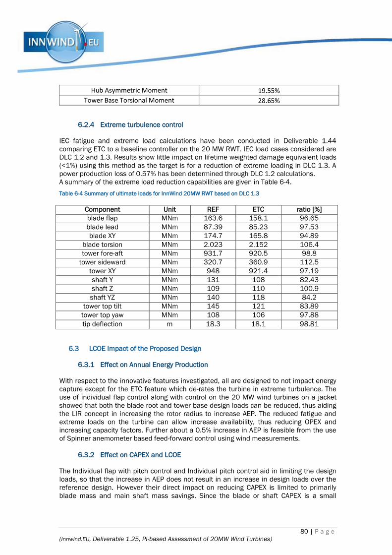
80 | P a g e
(Innwind.EU, Deliverable 1.25, PI-based Assessment of 20MW Wind Turbines)
Hub Asymmetric Moment 19.55%
Tower Base Torsional Moment 28.65%
6.2.4 Extreme turbulence control
IEC fatigue and extreme load calculations have been conducted in Deliverable 1.44
comparing ETC to a baseline controller on the 20 MW RWT. IEC load cases considered are
DLC 1.2 and 1.3. Results show little impact on lifetime weighted damage equivalent loads
(<1%) using this method as the target is for a reduction of extreme loading in DLC 1.3. A
power production loss of 0.57% has been determined through DLC 1.2 calculations.
A summary of the extreme load reduction capabilities are given in Table 6-4.
Table 6-4 Summary of ultimate loads for InnWind 20MW RWT based on DLC 1.3
Component Unit REF ETC ratio [%]
blade flap MNm 163.6 158.1 96.65
blade lead MNm 87.39 85.23 97.53
blade XY MNm 174.7 165.8 94.89
blade torsion MNm 2.023 2.152 106.4
tower fore-aft MNm 931.7 920.5 98.8
tower sideward MNm 320.7 360.9 112.5
tower XY MNm 948 921.4 97.19
shaft Y MNm 131 108 82.43
shaft Z MNm 109 110 100.9
shaft YZ MNm 140 118 84.2
tower top tilt MNm 145 121 83.89
tower top yaw MNm 108 106 97.88
tip deflection m 18.3 18.1 98.81
6.3 LCOE Impact of the Proposed Design
6.3.1 Effect on Annual Energy Production
With respect to the innovative features investigated, all are designed to not impact energy
capture except for the ETC feature which de-rates the turbine in extreme turbulence. The
use of individual flap control along with control on the 20 MW wind turbines on a jacket
showed that both the blade root and tower base design loads can be reduced, thus aiding
the LIR concept in increasing the rotor radius to increase AEP. The reduced fatigue and
extreme loads on the turbine can allow increase availability, thus reducing OPEX and
increasing capacity factors. Further about a 0.5% increase in AEP is feasible from the use
of Spinner anemometer based feed-forward control using wind measurements.
6.3.2 Effect on CAPEX and LCOE
The Individual flap with pitch control and Individual pitch control aid in limiting the design
loads, so that the increase in AEP does not result in an increase in design loads over the
reference design. However their direct impact on reducing CAPEX is limited to primarily
blade mass and main shaft mass savings. Since the blade or shaft CAPEX is a small

81 | P a g e
(Innwind.EU, Deliverable 1.25, PI-based Assessment of 20MW Wind Turbines)
portion of the overall CAPEX when including the substructure, a limited influence on the
overall CAPEX of less than 1% is seen from using active controls. However when the
combined with the LIR concept and wind observers for feed-forward control, a net
reduction in LCOE of at least 4% can be expected compared to the 20 MW reference,
primarily derived from the larger AEP.
6.4 Conclusions
A range of control features have been applied to the INNWIND 20 MW RWT, 20 MW RWT
on advanced steel jacket and 20 MW LIR on advanced steel jacket. In-plane damping and
tower damping are considered essential features for the investigated configuration and
together with CPC form a baseline control architecture for the 20 MW RWT. Further to this
IPC, IFPC-FB, IFPC-FF and ETC have been applied with reductions in loading quantified.
IPC and IFPC have been shown to results in similar levels of fatigue load reduction on the
blade roots but introduce slightly higher fatigue of the tower base.
IFC has been shown to lead to reduced extreme loading using intelligent shutdowns and
through reducing pitch angle asymmetries at the onset of pitch faults. There is also the
benefit of reduced pitch activity, though this has not been quantified for this study.
ETC has demonstrated reductions in extreme loading that occur in DLC 1.3 from extreme
turbulence, with the largest impacts on blade root bending and all RNA tilting loads.

82 | P a g e
(Innwind.EU, Deliverable 1.25, PI-based Assessment of 20MW Wind Turbines)
CHAPTER 7 SYNTHESIS AND CONCLUSIONS
The comparison of the studied concepts in terms of the Performance Indicators (PIs) set
for the INNWIND.EU project is presented in Table 7-1 and Table 7-2. The first Table presents
dimensional values of the PIs while the second shows percentage changes in comparison
to the PI values of the 20MW Reference Wind Turbine. The combined effect of the
rotor/drive train/support structure/control concepts is also included in the Tables.
The PI values used in the Tables may be slightly different than those presented in the
earlier chapters of the report. This is the result of a harmonization procedure including the
recalculation of all the PIs, whenever needed, with dedicated spreadsheets employing the
cost model version of Ref [10].
For a better appreciation of the 20MW designs we include in the Tables the relevant PI
values of the 10MW RWT. Moving from 10 to 20MW notable are the slight increase of the
wind farm capacity factor due to less wake effects for the same installed capacity and the
significant reduction of O&M cost from nearly 35 €/MWh to 28 €/MWh.
Table 7-1 Performance Indicators of the innovative concepts studied
ROTORComponent
Mass (tn)
Component
Cost (k€)
Overall CAPEX
(k€)
Turbine
CF
Wind Farm
CF
O&M
(€/MWh)
LCOE
(€/MWh)
RWT - 10MW 42 448 30,650 0.507 0.425 34.81 98.56
RWT - 20MW 118 1,274 64,550 0.508 0.437 28.08 93.22
Low Induction Rotor (LIR) 20MW 99 1,367 66,750 0.546 0.480 28.08 89.58
BTC Rotor 20MW (D = D RWT ) 108 1,163 64,000 0.508 0.438 28.08 92.67
DRIVE TRAIN & NACELLEComponent
Mass (tn)
Component
Cost (k€)
Overall CAPEX
(k€)
Turbine
CF
Wind Farm
CF
O&M
(€/MWh)
LCOE
(€/MWh)
RWT - 10MW 338 4,515 30,650 0.507 0.425 34.81 98.56
RWT - 20MW 914 11,300 64,550 0.508 0.437 28.08 93.22
PDD Generator 20MW 950 10,500 63,200 0.513 0.442 28.08 91.35
OFFSHORE SUPPORT STRUCTComponent
Mass (tn)
Component
Cost (k€)
Overall CAPEX
(k€)
Turbine
CF
Wind Farm
CF
O&M
(€/MWh)
LCOE
(€/MWh)
RWT - 10MW 1,920 9,497 30,650 0.507 0.425 34.81 98.56
RWT - 20MW 3,090 13,950 64,550 0.508 0.437 28.08 93.22
Advanced Jacket (AJ) 20MW 11,160 61,800 0.508 0.437 28.08 90.53
ADVANCED CONTROLComponent
Mass (tn)
Component
Cost (k€)
Overall CAPEX
(k€)
Turbine
CF
Wind Farm
CF
O&M
(€/MWh)
LCOE
(€/MWh)
RWT - 10MW 30,650 0.507 0.425 34.81 98.56
RWT - 20MW 64,550 0.508 0.437 28.08 93.22
Advanced Control (AC) 20MW 89.49
COMBINATIONSOverall CAPEX
(k€)
Turbine
CF
Wind Farm
CF
O&M
(€/MWh)
LCOE
(€/MWh)
RWT - 10MW 30,650 0.507 0.425 34.81 98.56
RWT - 20MW 64,550 0.508 0.437 28.08 93.22
LIR + BTC + PDD + AJ + AC (20MW) 62,100 0.551 0.485 28.08 80.74

83 | P a g e
(Innwind.EU, Deliverable 1.25, PI-based Assessment of 20MW Wind Turbines)
Table 7-2 Percentage improvement of PIs in comparison to the 20MW RWT
7.1 Blade Concepts
LIR concept (Chapter 2)
The new hybrid (glass-carbon) blade is lighter (16%) than the full-glass classically up-
scaled 20MW RWT blade but more expensive (7.3%). This is due to its longer span and the
use of expensive carbon. Nevertheless, the overall increase in turbine CAPEX is 3.4%
because in offshore wind the blades represent a small fraction of the turbine and support
structure cost. Despite the higher CAPEX the larger, less loaded rotor, increases the
turbine yield (capacity factor CF) by 7.5%. As stated earlier, a 4.5% comes from the LIR
planform and another 3% from the dedicated low lift profiles. Even more important is the
increase of the wind farm capacity factor by 9.7% due to the lower wake losses of LIR
rotors. This is the highest value achieved among the different rotor concepts. Overall, LIR
promises a 3.9% reduction of LCOE compared to the 20MW RWT.
Bend-Twist Coupled Rotor (Chapter 3)
The conclusions here regarding the impact of the BTC concept on LCOE are similar to
those extracted for 10MW designs. No real improvement in the cost of energy is expected
maintaining the reference rotor diameter. Such designs may reduce primary the fatigue
and secondary the ultimate loading of the blade itself but, also, of the support structure
having an indirect effect on CAPEX reduction which, however, is not taken into account in
the present context. The BTC blade is highly loaded (high Cp_max design) and 8.5% lighter
and cheaper than the RWT blade. The overall CAPEX and LCOE improvement is small (1%)
leading to an LCOE reduction of 0.6%. Due to the assumptions made we can consider that
BTC improvements can be superimposed to LIR summing up their individual impacts to all
PIs. Alternatively, the BTC concept could be used to increase the diameter of a Cp_max
ROTORComponent
Mass (Δ%)
Component
Cost (Δ%)
Overall CAPEX
(Δ%)
Turbine
CF (Δ%)
Wind Farm
CF (Δ%) O&M (Δ%) LCOE (Δ%)
Low Induction Rotor (LIR) 20MW -16.1% 7.3% 3.4% 7.5% 9.7% 0.0% -3.9%
BTC Rotor 20MW (D = D RWT ) -8.5% -8.7% -0.9% 0.1% 0.1% 0.0% -0.6%
DRIVE TRAIN & NACELLEComponent
Mass (Δ%)
Component
Cost (Δ%)
Overall CAPEX
(Δ%)
Turbine
CF (Δ%)
Wind Farm
CF (Δ%) O&M (Δ%) LCOE (Δ%)
PDD Generator 20MW 3.9% -7.1% -2.1% 1.0% 1.1% 0.0% -2.0%
OFFSHORE SUPPORT STRUCTComponent
Mass (Δ%)
Component
Cost (Δ%)
Overall CAPEX
(Δ%)
Turbine
CF (Δ%)
Wind Farm
CF (Δ%) O&M (Δ%) LCOE (Δ%)
Advanced Jacket 20MW -20.0% -4.3% 0.0% 0.0% 0.0% -2.9%
ADVANCED CONTROLComponent
Mass (tn)
Component
Cost (k€)
Overall CAPEX
(k€)
Turbine
CF
Wind Farm
CF
O&M
(€/MWh)
LCOE
(€/MWh)
Advanced Control (AC) 20MW -4.0%
COMBINATIONS
Overall
CAPEX/MW
(Δ%)
Turbine
CF (Δ%)
Wind Farm
CF (Δ%) O&M (Δ%) LCOE (Δ%)
RWT - 10MW -5.0% -0.2% -2.8% 24.0% 5.7%
LIR + BTC + PDD + AJ + AC 20MW -3.8% 8.6% 10.9% 0.0% -13.4%

84 | P a g e
(Innwind.EU, Deliverable 1.25, PI-based Assessment of 20MW Wind Turbines)
rotor maintaining the loads to their reference level. If this is possible for the design loads
(ultimate and fatigue) of the individual load carrying components, it would also lead to an
increased turbine capacity factor without using the LIR concept. Overall LIR+BTC or BLT
alone can offer an LCOE reduction of 4 to 5%.
7.2 Drive Train Concepts
Magnetic Pseudo Direct Drive (PDD) (Chapter 4)
The PDD generator with highly efficient power electronics promises a good LCOE
performance (2 % lower than the reference) combined with a significant nacelle/drive train
cost reduction of 7%. The nacelle mass is slightly increased by 4% while the capacity factor
increases by 1.1 % which, along with the reduced CAPEX, is the reason of LCOE
improvement. The improved capacity factor comes as a combination of the highly efficient
20MW PDD generator (98.5% at full load) and the highly efficient power electronics.
7.3 Support Structure Concepts
Bottom Mounted Offshore Support Structure (Chapter 5)
An advanced design/manufacturing of the 20MW RWT jacket is expected to reduce the
original cost of ~14 M€ by 20%. Such a reduction would decrease the overall CAPEX by
4.3% translated to 2.9% reduction of the LCOE.
7.4 Advanced Control
Advanced Control in 20MW (Chapter 6)
An LCOE drop of 4% can be expected due to the mitigation of design loads of the turbine
and its support structure offered by advanced control. In the present context advanced
control was mainly targeted in reducing blade than support structure loads. Such a
reduction can be used for increasing the rotor diameter and improve LCOE through better
energy capturing. Alternatively, one can target on the reduction of the support structure
fatigue loads which are the design drivers of the jacket. For jacket structures load
reduction is nearly proportional to mass reduction. Since the offshore turbine support
structure has a significant contribution to CAPEX, the reduction of the jacket fatigue loads
through advanced control can also lead to an LCOE reduction of order 4% without
increasing rotor diameter.
7.5 Combination of Innovative Concepts and Overall Expectations
A simplified methodology for estimating the combined performance of the researched
concepts would sum-up the percentage gains of the individual innovations as soon as they
can be considered independent from each other. The combination of all innovative
concepts studied is given in the lower parts of the PI Tables.
For bottom mounted designs at INNWIND.EU 20MW RWT conditions the following
expectations regarding LCOE reduction look reasonable:
Low induction rotors with conventional inner structure 4.0%
Aeroelastically tailored rotors (adding on LIR) 0.5%
Drive train (reduced CAPEX, increased efficiency) 2.0%
Advanced Jacket 3.0%

85 | P a g e
(Innwind.EU, Deliverable 1.25, PI-based Assessment of 20MW Wind Turbines)
Advanced control 4%
Expected Overall LCOE reduction ~14%
Starting from the EWII LCOE value of 106.93 €/MWh corresponding to 5MW turbine sizes,
and considering more realistic than the EWII O&M costs this time, this number dropped at
98.56 €/MWh (8.5% reduction) for the 10MW RWT and 93.22 €/MWh (14.7% reduction)
for the 20MW RWT. These reductions were due to the larger turbine sizes along with the
use of a lightweight rotor with thick profiles and the shift from traditional three-stage
geared drive trains to medium speed single-stage drive while employing state of the art
designed and manufactured jackets. An additional 14% reduction of LCOE can be
expected for both 10 and 20MW designs, thanks to the advanced concepts researched in
INNWIND.EU, getting LCOE close to 80 €/MWh for 20MW turbines (and 85 €/MWh for
10MW turbines).

86 | P a g e
(Innwind.EU, Deliverable 1.25, PI-based Assessment of 20MW Wind Turbines)
REFERENCES
[1] INNWIND.EU Deliverable 1.25a, 20MW Reference Wind Turbine, Aeroelastic Data of the
Onshore Version.
[2] INNWIND.EU Deliverable 1.25b.
[3] INNWIND.EU Deliverable 1.22.
[4] P.K. Chaviaropoulos, J. Beurskens and S.Voutsinas,” Moving towards Large(r) Rotors – Is that
a good idea?”, Proc. EWEA 2013 Conference, Vienna, 2013.
[5] P.K. Chaviaropoulos and G. Sieros, “Design of Low Induction Rotors for use in large offshore
wind farms”, Proc. Scientific Track, EWEA 2014, Barcelona, 2014.
[6] P.K. Chaviaropoulos, G.Sieros, J.M. Prospathopoulos, K. Diakakis and S.G. Voutsinas, “Design
and CFD-based Performance Verification of a Family of Low-Lift Airfoils”, Proc. EWEA 2015,
Paris, 2015.
[7] INNWIND.EU Deliverable 2.12, New Airfoils for High Rotational Speed Wind Turbines, 2015.
[8] INNWIND.EU Deliverable 2.14.
[9] INNWIND.EU Deliverable 1.24.
[10] INNWIND.EU Deliverable 1.23.
[11] Bottasso C.L., Campagnolo F., Croce A., Tibaldi C., “Optimization-based study of bend–twist
coupled rotor blades for passive and integrated passive/active load alleviation”, Wind Energy,
Vol. 16, N.8, p1149-1166, 2013. DOI: 10.1002/we.1543 (2013)..
[12] Zahle, F., Tibaldi, C., Verelst, D. R., Bak, C., Bitche, R., and Blasques, J. P. A. A., Aero-Elastic
Optimization of a 10MW Wind Turbine, Proceedings of the 33rd Wind Energy Symposium ,
Kissimmee, Florida, U.S.A., 2015.
[13] Lobitz DW, Veers PS, Eisler GR, Laino DJ, Migliore PG, Bir G. The Use of Twist-Coupled Blades
to Enhance the Performance of Horizontal Axis Wind Turbines. Sandia Report SAND 2001-
1303, Sandia National Laboratories, Albuquerque, NM, May 2001..
[14] Lobitz D, Veers PS, Laino D. Performance of twist-coupled blades on variable speed rotors.
AIAA 2000-0062, 2000 ASME Wind Energy Symposium, Reno, January 10–13, 2000..
[15] A.Croce, Deliverable D2_22_PoliMI_16July2015.txt.
[16] P. Bortolotti, C. L. Bottasso and A. Croce, “Combined preliminary-detailed design of wind
turbines,” Wind Energy Science, vol. 1, pp. 71-88, 2016.
[17] Bottasso CL, Croce A. Cp-Lambda: User’s Manual. Dipartimento di Ingegneria Aerospaziale,
Politecnico di Milano, 2006–2011..
[18] IEC 61400-1. Wind turbines – Part 1: Design Requirements, 2005.
[19] Bottasso C.L., Campagnolo F., Croce A., “Multi-Disciplinary Constrained Optimization of Wind
Turbines”, Multibody System Dynamics, Vol. 27, N. 1, p. 21-53, 2012, ISSN: 1384-5640, doi:
10.1007/s11044-011-9271-x (2012)..
[20] INNWIND.EU Deliverable 4.36.
[21] “DNVGL-ST-0126, Support structures for wind turbines, 2016”.
[22] “DNVGL-RP-C203, Fatigue Design of offshore steel structures, 2016”.
[23] J. Serrano-González, “Technological evolution of onshore wind turbines-a market-based
analysis,” Wind Energy, 2016.
[24] W. H. Lio, “Fundamental performance similarities between individual pitch control strategies
for wind turbines,” International Journal of Control, vol. 90, no. 1, 2017.
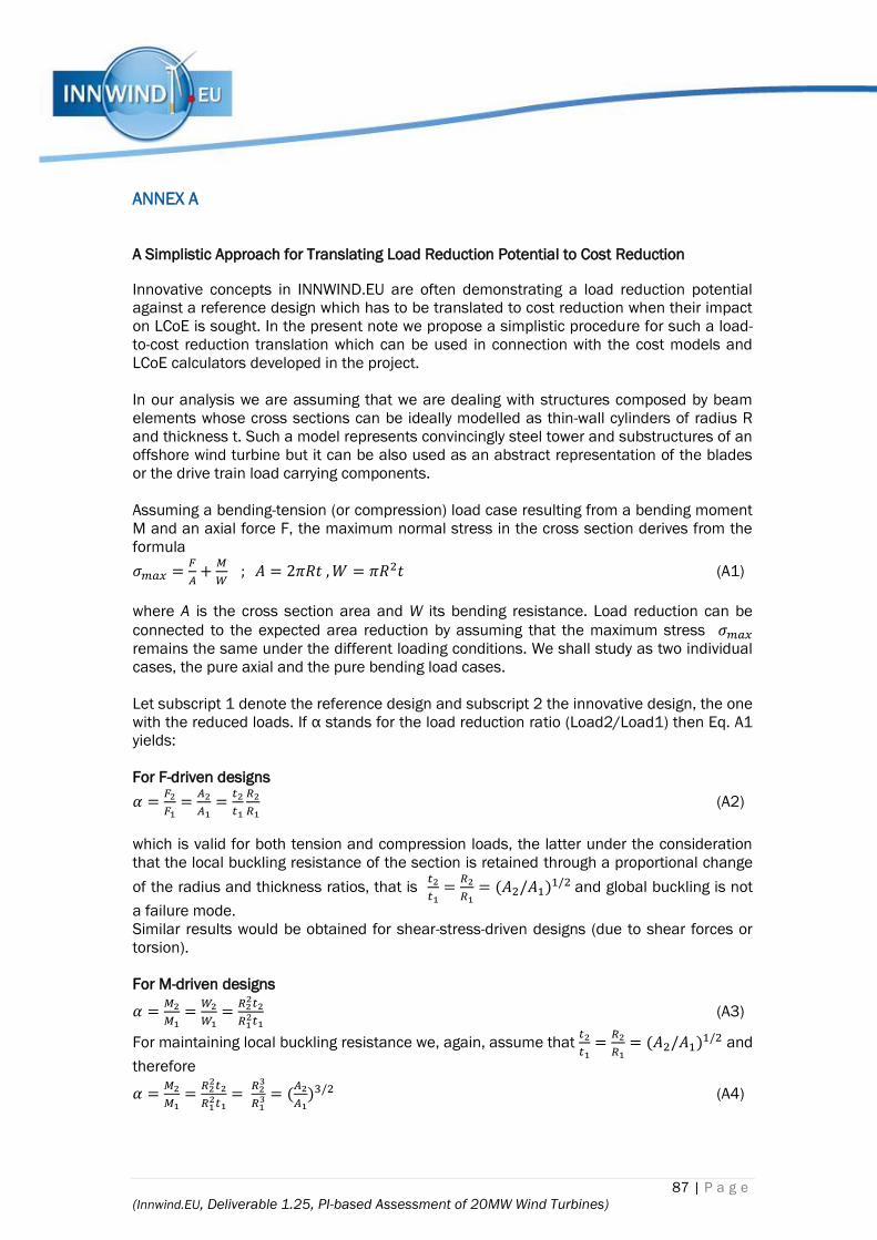
87 | P a g e
(Innwind.EU, Deliverable 1.25, PI-based Assessment of 20MW Wind Turbines)
ANNEX A
A Simplistic Approach for Translating Load Reduction Potential to Cost Reduction
Innovative concepts in INNWIND.EU are often demonstrating a load reduction potential
against a reference design which has to be translated to cost reduction when their impact
on LCoE is sought. In the present note we propose a simplistic procedure for such a load-
to-cost reduction translation which can be used in connection with the cost models and
LCoE calculators developed in the project.
In our analysis we are assuming that we are dealing with structures composed by beam
elements whose cross sections can be ideally modelled as thin-wall cylinders of radius R
and thickness t. Such a model represents convincingly steel tower and substructures of an
offshore wind turbine but it can be also used as an abstract representation of the blades
or the drive train load carrying components.
Assuming a bending-tension (or compression) load case resulting from a bending moment
M and an axial force F, the maximum normal stress in the cross section derives from the
formula
𝜎𝑚𝑎𝑥 =𝐹
𝐴+
𝑀
𝑊 ; 𝐴 = 2𝜋𝑅𝑡 , 𝑊 = 𝜋𝑅2𝑡 (A1)
where A is the cross section area and W its bending resistance. Load reduction can be
connected to the expected area reduction by assuming that the maximum stress 𝜎𝑚𝑎𝑥
remains the same under the different loading conditions. We shall study as two individual
cases, the pure axial and the pure bending load cases.
Let subscript 1 denote the reference design and subscript 2 the innovative design, the one
with the reduced loads. If α stands for the load reduction ratio (Load2/Load1) then Eq. A1
yields:
For F-driven designs
𝛼 =𝐹2
𝐹1=
𝐴2
𝐴1=
𝑡2
𝑡1
𝑅2
𝑅1 (A2)
which is valid for both tension and compression loads, the latter under the consideration
that the local buckling resistance of the section is retained through a proportional change
of the radius and thickness ratios, that is 𝑡2
𝑡1=
𝑅2
𝑅1= (𝐴2/𝐴1)1/2 and global buckling is not
a failure mode.
Similar results would be obtained for shear-stress-driven designs (due to shear forces or
torsion).
For M-driven designs
𝛼 =𝑀2
𝑀1=
𝑊2
𝑊1=
𝑅22𝑡2
𝑅12𝑡1
(A3)
For maintaining local buckling resistance we, again, assume that 𝑡2
𝑡1=
𝑅2
𝑅1= (𝐴2/𝐴1)1/2 and
therefore
𝛼 =𝑀2
𝑀1=
𝑅22𝑡2
𝑅12𝑡1
= 𝑅2
3
𝑅13 = (
𝐴2
𝐴1)3/2 (A4)
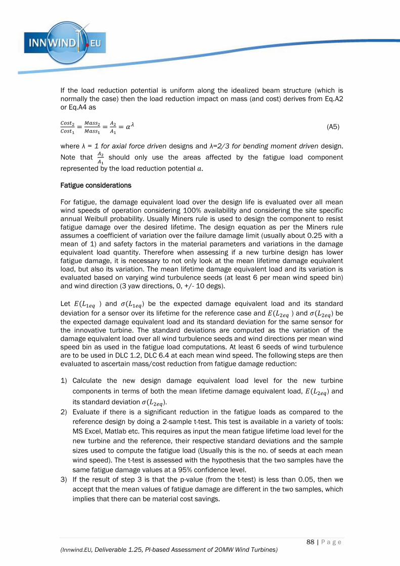
88 | P a g e
(Innwind.EU, Deliverable 1.25, PI-based Assessment of 20MW Wind Turbines)
If the load reduction potential is uniform along the idealized beam structure (which is
normally the case) then the load reduction impact on mass (and cost) derives from Eq.A2
or Eq.A4 as
𝐶𝑜𝑠𝑡2
𝐶𝑜𝑠𝑡1=
𝑀𝑎𝑠𝑠2
𝑀𝑎𝑠𝑠1=
𝐴2
𝐴1= 𝛼𝜆 (A5)
where λ = 1 for axial force driven designs and λ=2/3 for bending moment driven design.
Note that 𝐴2
𝐴1 should only use the areas affected by the fatigue load component
represented by the load reduction potential 𝑎.
Fatigue considerations
For fatigue, the damage equivalent load over the design life is evaluated over all mean
wind speeds of operation considering 100% availability and considering the site specific
annual Weibull probability. Usually Miners rule is used to design the component to resist
fatigue damage over the desired lifetime. The design equation as per the Miners rule
assumes a coefficient of variation over the failure damage limit (usually about 0.25 with a
mean of 1) and safety factors in the material parameters and variations in the damage
equivalent load quantity. Therefore when assessing if a new turbine design has lower
fatigue damage, it is necessary to not only look at the mean lifetime damage equivalent
load, but also its variation. The mean lifetime damage equivalent load and its variation is
evaluated based on varying wind turbulence seeds (at least 6 per mean wind speed bin)
and wind direction (3 yaw directions, 0, +/- 10 degs).
Let 𝐸(𝐿1𝑒𝑞 ) and 𝜎(𝐿1𝑒𝑞) be the expected damage equivalent load and its standard
deviation for a sensor over its lifetime for the reference case and 𝐸(𝐿2𝑒𝑞 ) and 𝜎(𝐿2𝑒𝑞) be
the expected damage equivalent load and its standard deviation for the same sensor for
the innovative turbine. The standard deviations are computed as the variation of the
damage equivalent load over all wind turbulence seeds and wind directions per mean wind
speed bin as used in the fatigue load computations. At least 6 seeds of wind turbulence
are to be used in DLC 1.2, DLC 6.4 at each mean wind speed. The following steps are then
evaluated to ascertain mass/cost reduction from fatigue damage reduction:
1) Calculate the new design damage equivalent load level for the new turbine
components in terms of both the mean lifetime damage equivalent load, 𝐸(𝐿2𝑒𝑞) and
its standard deviation 𝜎(𝐿2𝑒𝑞).
2) Evaluate if there is a significant reduction in the fatigue loads as compared to the
reference design by doing a 2-sample t-test. This test is available in a variety of tools:
MS Excel, Matlab etc. This requires as input the mean fatigue lifetime load level for the
new turbine and the reference, their respective standard deviations and the sample
sizes used to compute the fatigue load (Usually this is the no. of seeds at each mean
wind speed). The t-test is assessed with the hypothesis that the two samples have the
same fatigue damage values at a 95% confidence level.
3) If the result of step 3 is that the p-value (from the t-test) is less than 0.05, then we
accept that the mean values of fatigue damage are different in the two samples, which
implies that there can be material cost savings.
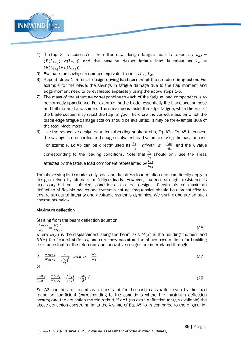
89 | P a g e
(Innwind.EU, Deliverable 1.25, PI-based Assessment of 20MW Wind Turbines)
4) If step 3 is successful, then the new design fatigue load is taken as 𝐿𝑑2 =
(𝐸(𝐿2𝑒𝑞)+ 𝜎(𝐿2𝑒𝑞)) and the baseline design fatigue load is taken as 𝐿𝑑1 =
(𝐸(𝐿1𝑒𝑞)+ 𝜎(𝐿1𝑒𝑞))
5) Evaluate the savings in damage equivalent load as 𝐿𝑑2-𝐿𝑑1
6) Repeat steps 1 -5 for all design driving load sensors of the structure in question. For
example for the blade, the savings in fatigue damage due to the flap moment and
edge moment need to be evaluated separately using the above steps 1-5.
7) The mass of the structure corresponding to each of the fatigue load components is to
be correctly apportioned. For example for the blade, essentially the blade section nose
and tail material and some of the shear webs resist the edge fatigue, while the rest of
the blade section may resist the flap fatigue. Therefore the correct mass on which the
blade edge fatigue damage acts on should be evaluated. It may be for example 30% of
the total blade mass.
8) Use the respective design equations (bending or shear etc), Eq. A3 - Eq. A5 to convert
the savings in one particular damage equivalent load value to savings in mass or cost.
For example, Eq.A5 can be directly used as 𝐴2
𝐴1= 𝛼𝜆with 𝛼 =
𝐿𝑑2
𝐿𝑑1 and the λ value
corresponding to the loading conditions. Note that 𝐴2
𝐴1 should only use the areas
affected by the fatigue load component represented by 𝐿𝑑2
𝐿𝑑1
The above simplistic models rely solely on the stress-load relation and can directly apply in
designs driven by ultimate or fatigue loads. However, material strength resistance is
necessary but not sufficient conditions in a real design. Constraints on maximum
deflection of flexible bodies and system’s natural frequencies should be also satisfied to
ensure structural integrity and desirable system’s dynamics. We shall elaborate on such
constraints below.
Maximum deflection
Starting from the beam deflection equation 𝑑2𝑤(𝑥)
𝑑𝑥2 =𝑀(𝑥)
𝐸𝐼(𝑥) (A6)
where 𝑤(𝑥) is the displacement along the beam axis 𝑀(𝑥) is the bending moment and
𝐸𝐼(𝑥) the flexural stiffness, one can show based on the above assumptions for buckling
resistance that for the reference and innovative designs are interrelated through:
𝑑 =𝑤2𝑚𝑎𝑥
𝑤1𝑚𝑎𝑥=
𝛼
(𝐴2𝐴1
)2 𝑤𝑖𝑡ℎ 𝛼 =
𝑀2
𝑀1 (A7)
or
𝐶𝑜𝑠𝑡2
𝐶𝑜𝑠𝑡1=
𝑀𝑎𝑠𝑠2
𝑀𝑎𝑠𝑠1= (
𝐴2
𝐴1) = (
𝛼
𝑑)1/2 (A8)
Eq. A8 can be anticipated as a constraint for the cost/mass ratio driven by the load
reduction coefficient (corresponding to the conditions where the maximum deflection
occurs) and the deflection margin ratio d. If d=1 (no extra deflection margin available) the
above deflection constraint limits the λ value of Eq. A5 to ½ compared to the original M-
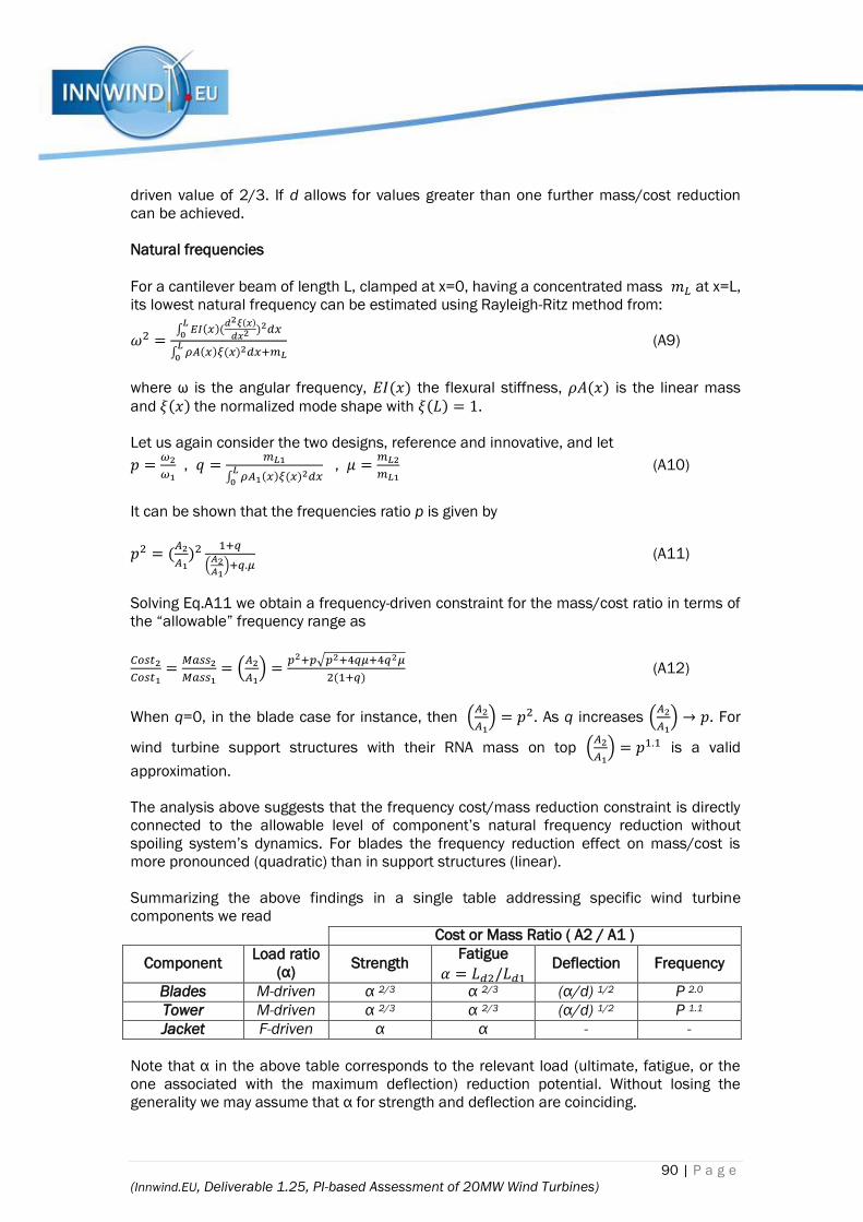
90 | P a g e
(Innwind.EU, Deliverable 1.25, PI-based Assessment of 20MW Wind Turbines)
driven value of 2/3. If d allows for values greater than one further mass/cost reduction
can be achieved.
Natural frequencies
For a cantilever beam of length L, clamped at x=0, having a concentrated mass 𝑚𝐿 at x=L,
its lowest natural frequency can be estimated using Rayleigh-Ritz method from:
𝜔2 =∫ 𝐸𝐼(𝑥)(
𝑑2𝜉(𝑥)
𝑑𝑥2 )2𝐿
0𝑑𝑥
∫ 𝜌𝐴(𝑥)𝜉(𝑥)2𝐿
0𝑑𝑥+𝑚𝐿
(A9)
where ω is the angular frequency, 𝐸𝐼(𝑥) the flexural stiffness, 𝜌𝛢(𝑥) is the linear mass
and 𝜉(𝑥) the normalized mode shape with 𝜉(𝐿) = 1.
Let us again consider the two designs, reference and innovative, and let
𝑝 =𝜔2
𝜔1 , 𝑞 =
𝑚𝐿1
∫ 𝜌𝐴1(𝑥)𝜉(𝑥)2𝐿
0𝑑𝑥
, 𝜇 =𝑚𝐿2
𝑚𝐿1 (A10)
It can be shown that the frequencies ratio p is given by
𝑝2 = (𝐴2
𝐴1)2 1+𝑞
(𝐴2𝐴1
)+𝑞.𝜇 (A11)
Solving Eq.A11 we obtain a frequency-driven constraint for the mass/cost ratio in terms of
the “allowable” frequency range as
𝐶𝑜𝑠𝑡2
𝐶𝑜𝑠𝑡1=
𝑀𝑎𝑠𝑠2
𝑀𝑎𝑠𝑠1= (
𝐴2
𝐴1) =
𝑝2+𝑝√𝑝2+4𝑞𝜇+4𝑞2𝜇
2(1+𝑞) (A12)
When q=0, in the blade case for instance, then (𝐴2
𝐴1) = 𝑝2. As q increases (
𝐴2
𝐴1) → 𝑝. For
wind turbine support structures with their RNA mass on top (𝐴2
𝐴1) = 𝑝1.1 is a valid
approximation.
The analysis above suggests that the frequency cost/mass reduction constraint is directly
connected to the allowable level of component’s natural frequency reduction without
spoiling system’s dynamics. For blades the frequency reduction effect on mass/cost is
more pronounced (quadratic) than in support structures (linear).
Summarizing the above findings in a single table addressing specific wind turbine
components we read
Cost or Mass Ratio ( A2 / A1 )
Component Load ratio
(α) Strength
Fatigue
𝛼 = 𝐿𝑑2/𝐿𝑑1 Deflection Frequency
Blades M-driven α 2/3 α 2/3 (α/d) 1/2 P 2.0
Tower M-driven α 2/3 α 2/3 (α/d) 1/2 P 1.1
Jacket F-driven α α - -
Note that α in the above table corresponds to the relevant load (ultimate, fatigue, or the
one associated with the maximum deflection) reduction potential. Without losing the
generality we may assume that α for strength and deflection are coinciding.

91 | P a g e
(Innwind.EU, Deliverable 1.25, PI-based Assessment of 20MW Wind Turbines)
Application examples and synthesis
Consider an application example where for an F-driven design a specific new concept can
reduce the ultimate axial force on a load carrying component by 20%. Then α=0.8 and,
from Eq.A5 for λ=1, this results to a mass (cost) ratio of 80% corresponding to 20% cost
reduction. Here the cost-load benefit is 100%. On the other hand, a 20% ultimate moment
reduction of an M-driven design corresponding to α=0.8 leads (Eq.A5 for λ=2/3) to a mass
ratio of 0.86 and therefore to 14% cost reduction. In this case the cost-load benefit is
lower, 14/20=70%. These cost benefit values are valid when no deflection or frequency
constraints are imposed.
Blades and tubular towers can be considered as moment driven designs and therefore
they can be handled with λ=2/3. Blades are subjected to deflection and frequency
constraints. If no extra deflection margin is available (d=1) than their λ value drops from
2/3 to ½ and for the above examined case of α=0.8 the minimum allowable mass ratio is
0.894 and the cost-load benefit can go up to 53%. The difference from 53% to 70% can be
only recovered by allowing for an increased (estimated to 5% by solving α2/3 = (α/d)½ for d)
blade deflection. Regarding the blade frequency constraint a full exploitation of the cost
load benefit (λ=2/3) for α=0.8 would result to a p = 0.93 value corresponding to 7%
reduction of its lowest (1st flap) frequency which is a rather affordable number
For 10+ MW bottom-fixed offshore turbines considered here one can probably exploit fully
the cost reduction benefit of λ=2/3 corresponding to a 5% increase of tower-top maximum
deflection for α=0.8 does not seem to be a problem, while the frequency reduction of 7%
for the same α value is rather beneficial for the design in terms of preventing the tower
excitation in the variable speed regime of turbine normal operation.
Multi-member truss-type constructions like jackets are rather axial force driven designs
and a λ value closer to 1 can be used for them. Here, the deflection constraint does not
seem to be a problem thanks to the high stiffness of the jacket while the frequency
reduction is again beneficial for the large turbines of our consideration.
Clearly, the proposed model is very crude as it is based on many assumptions and
simplifications. Nevertheless it provides some basic evidence on how load reduction can
be translated to mass reduction and what the expected cost-load benefit could roughly be.

PROPRIETARY RIGHTS STATEMENT
This document contains information, which is proprietary to the “INNWIND.EU” Consortium. Neither this document nor
the information contained herein shall be used, duplicated or communicated by any means to any third party, in whole
or in parts, except with prior written consent of the “INNWIND.EU” consortium.
20 MW Reference Wind Turbine
Aeroelastic data of the onshore version of the turbine
April 2016
Agreement n.: 308974
Duration November 2012 – October 2017
DTU Wind
The research leading to these results has received funding from
the European Community’s Seventh Framework Programme
under grant agreement
2 | P a g e
Innwind.EU, Deliverable 1.25, 20MW Reference Wind Turbine
Document information
Document Name: 20 MW Reference Wind Turbine
Aeroelastic data of the onshore version
Document
Number:
Deliverable D 1.25 (a)
Author: Panagiotis Chaviaropoulos, Alkis Milidis (NTUA)
Document Type Report
Dissemination
level
PU
Review: Anand Natarajan (DTU)
Date: April 2016
WP: WP1: Conceptual Design
Task: Task 1.2: Assessment of Innovation at the Subsystem Level
Approval: Approved by WP Leader

3 | P a g e
Innwind.EU, Deliverable 1.25, 20MW Reference Wind Turbine
TABLE OF CONTENTS
Aeroelastic data of the onshore version of the turbine .................................................................... 1
TABLE OF CONTENTS ............................................................................................................................. 3
INTRODUCTION ....................................................................................................................................... 4
CHALLENGES IN DESIGNING FOR 20 MW ............................................................................................ 5
CLASSICAL UPSCALING TECHNIQUES ................................................................................................... 9 3.1 Blades .................................................................................................................................... 9
3.2 Tower ................................................................................................................................... 12
DEVIATING FROM CLASSICAL UPSCALING .......................................................................................... 13 4.1 Rotor .................................................................................................................................... 13
4.2 Nacelle – Hub ...................................................................................................................... 13
4.3 Drive train ............................................................................................................................ 13
4.4 Tower ................................................................................................................................... 13
4.5 Control ................................................................................................................................. 14
4.6 Design summary ................................................................................................................. 15
FIRST ASSESSMENT OF THE 20 MW DESIGN..................................................................................... 16 5.1 Blade natural frequencies .................................................................................................. 16
5.2 Turbine natural frequencies ............................................................................................... 16
5.3 Blade root ultimate loads from DLC 6.2 ............................................................................ 17
5.4 Tower bottom ultimate loads from DLC 6.2 ...................................................................... 18
5.5 Blade root fatigue loads from DLC 1.2 .............................................................................. 21
5.6 Tower bottom fatigue loads from DLC 1.2 ......................................................................... 23
SUMMARY ............................................................................................................................................. 27
REFERENCES ........................................................................................................................................ 28
APPENDIX I: CONTROL PARAMETERS OF THE 20MW RWT ................................................................ 29
APPENDIX IΙ: FATIGUE RESULTS FOR ALL TOWER VERSIONS OF THE 20MW RWT .......................... 34
4 | P a g e
Innwind.EU, Deliverable 1.25, 20MW Reference Wind Turbine
INTRODUCTION
In this document we present the land version of the 20 MW Reference Wind Turbine of
INNWIND.EU project and we present the methodologies used for defining its aeroelastic data
needed for its performance and loading calculations.
The 20MW RWT is not designed from scratch but it derives from the upscaling of the 10MW DTU
RWT. Contrary to the 10MW RWT which was an IEC-61400 Class IA design, the 20MW RWT is
designed for Class IC. This is mainly expected to affect the fatigue loads which are the design
drivers of some critical turbine subcomponents, among them its offshore support system, which
have significant contribution to the turbine CAPEX (and, therefore LCoE).
Classical upscaling techniques are first used for configuring all turbine subsystems.. In a next step
the initial data are trimmed to incorporate mass (cost) reduction expectations due to technology
advancement and designing for a lower turbulent subclass. This is resulting in a 252.2m diameter
20MW rotor designed for an optimal TSR of 7.5, spinning with a tip speed of 90m/s and placed at
a hub height exceeding 165m. The 122m long blades of the 20MW are expected to weight 118t
each, while the nacelle mass is expected to be heavier than 1000t.
The design of a 20 MW offshore turbine includes further challenges regarding the proper selection
of systems first global frequency (related to the support structure design) in connection to the
variable speed schedule of the turbine which is essential for its high performance. Further
deviations from classical upscaling are thus effected to avoid the cross-cutting of the rotor 3P
frequency with the 1st global frequency at wind speeds that are critical for the turbine performance
and loading. This is accomplished through a slight increase of the rotor Tip Speed Ratio and a
parallel increase of the tower height by 12 meters.
The design summary of the turbine is cross compared against that of the 10MW RWT. The
aeroelastic data of the turbine and its subcomponents are given in XLS spreadsheets
accompanying this report. There are three such spreadsheets addressing three alternative towers.
This is an option discussed and agreed with WP4 which will design the 20MW jacket.
Further, this report makes a first evaluation of the 20MW RWT (onshore version) in terms of its
dynamics (natural frequencies of the system) and loads. Blade and tower root ultimate and fatigue
loads are presented for two relevant IEC-61400 DLCs. The tower bottom loads are a prerequisite
for the jacket design.
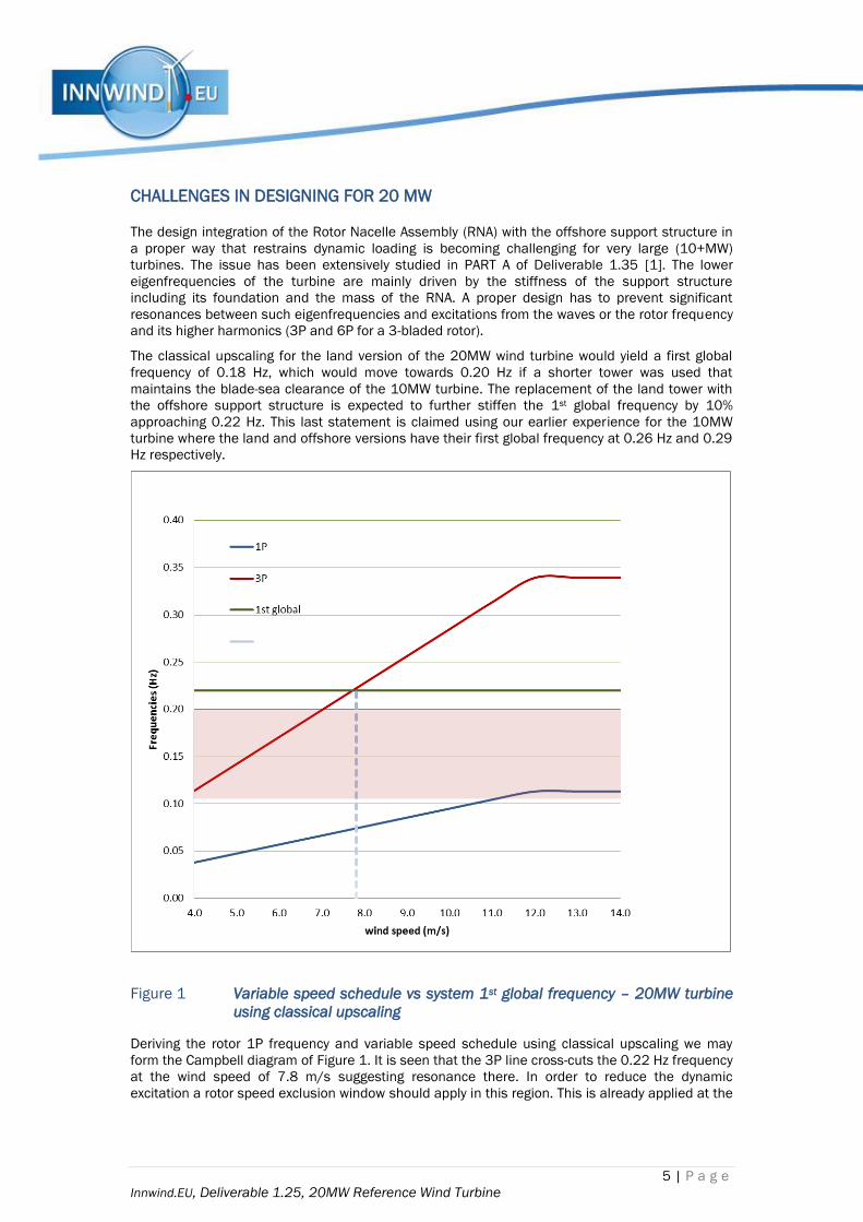
5 | P a g e
Innwind.EU, Deliverable 1.25, 20MW Reference Wind Turbine
CHALLENGES IN DESIGNING FOR 20 MW
The design integration of the Rotor Nacelle Assembly (RNA) with the offshore support structure in
a proper way that restrains dynamic loading is becoming challenging for very large (10+MW)
turbines. The issue has been extensively studied in PART A of Deliverable 1.35 [1]. The lower
eigenfrequencies of the turbine are mainly driven by the stiffness of the support structure
including its foundation and the mass of the RNA. A proper design has to prevent significant
resonances between such eigenfrequencies and excitations from the waves or the rotor frequency
and its higher harmonics (3P and 6P for a 3-bladed rotor).
The classical upscaling for the land version of the 20MW wind turbine would yield a first global
frequency of 0.18 Hz, which would move towards 0.20 Hz if a shorter tower was used that
maintains the blade-sea clearance of the 10MW turbine. The replacement of the land tower with
the offshore support structure is expected to further stiffen the 1st global frequency by 10%
approaching 0.22 Hz. This last statement is claimed using our earlier experience for the 10MW
turbine where the land and offshore versions have their first global frequency at 0.26 Hz and 0.29
Hz respectively.
Figure 1 Variable speed schedule vs system 1st global frequency – 20MW turbine
using classical upscaling
Deriving the rotor 1P frequency and variable speed schedule using classical upscaling we may
form the Campbell diagram of Figure 1. It is seen that the 3P line cross-cuts the 0.22 Hz frequency
at the wind speed of 7.8 m/s suggesting resonance there. In order to reduce the dynamic
excitation a rotor speed exclusion window should apply in this region. This is already applied at the

6 | P a g e
Innwind.EU, Deliverable 1.25, 20MW Reference Wind Turbine
10MW RWT offshore turbine, at speed range approximately ±10% around 6 rpm. The extent of the
exclusion zone is a trade-off between loss in energy capture (due to deviation from the optimal
TSR) and fatigue loading due to dynamic excitation of the support structure.
Both energy capture losses and fatigue loads are reduced when the resonance wind speed gets
lower. This can be done by increasing the rotor speed or reducing the 1st global frequency or a
combination of both.
Increasing the rotational speed of an existing blade (or operating it at a different TSR than its
design value) is also having consequences on power production. Table 1 presents a study of the
effect of rotor speed (through a TSR multiplier, noted as RPM x) and the late start of the variable
speed schedule (above a given wind speed, noted as VS>value) on the capacity factor (CF) of a
single turbine. The calculations have been performed assuming the INNWIND.EU reference site
conditions (Rayleigh distribution with mean annual wind speed 9.3 m/s). The first two rows
confirm that the 10MW RWT and the classically up-scaled 20MW turbine do have the same
capacity factor. The third row shows that if the variable speed operation is also effected in the
wind speed interval 4-7m/s this would result to a rather small increase of CF from 50.25% to
50.48%. The fourth row suggests that a 5% over-speeding of the reference rotor has a minor effect
on CF reduction due to off-design operation. This effect is almost tripled when the over-speed
becomes 10%.
Table 1 Off-optimal-λ consequences to the single turbine capacity factor
A 5% over-speed increases the tip speed of the blades from the original value of ~90m/s to
~95m/s. Further tip speed increase will result to higher power losses and burden corrosion
effects. Thus the selection made for the 20MW RWT rotor is to use the geometrically up-scaled
10MW blade rotating 5% faster.
Table 2 shows the operating characteristics of the 20MW RWT rotor. Note that the TSR value in
the variable speed range is now 7.91 (from 7.53) and the tip speed 94.12 m/s.
Reducing the 1st global frequency is more complicated. Ideally we would prefer to have a 1st global
frequency of the offshore turbine close to 0.20 Hz. Higher values would move tower-rotor
resonance at higher wind speeds while lower values might increase wave excitation loads. To do
that the land version of the turbine should have an even lower 1st global frequency. At the tower
design level this can be done either by increasing the tower height or increasing the tower mass.
Through an investigation which is presented in a later section of the report, the decided to
increase the tower height and have a blade-sea water clearance of 42m instead of the 30m of the
10MW RWT. Although a longer tower increases the ultimate and fatigue moments on the support
structure this will be counterbalanced through the suppression of the dynamic loads (rotor-support
structure interaction) and the reduction of turbulence induced loads (both ultimate and fatigue)
since the design class is now IC compared to the IA of the 10MW RWT.
RPM x
Prated
(MW)
Pmean
(MW) CF (%)
Max Flap
Moment
(kNm)
10 MW RWT (VS > 7 m/s) 1.00 10 5.025 50.25% 29091.75
20 MW Upscaled (VS > 7 m/s) 1.00 20 10.051 50.25% 82283.96
20 MW Upscaled (VS > 4 m/s) 1.00 20 10.095 50.48% 82299.42
20 MW Upscaled (VS > 4 m/s) 1.05 20 10.071 50.36% 85607.28
20 MW Upscaled (VS > 4 m/s) 1.10 20 10.013 50.07% 88698.62
20 MW Upscaled (VS >7 m/s) 1.10 20 9.920 49.60% 88683.79

7 | P a g e
Innwind.EU, Deliverable 1.25, 20MW Reference Wind Turbine
Table 2 Operational characteristics of the 20 MW RWT
The final selection of the 20MW RWT tower properties will be made after the 20MW RWT jacket is
designed by WP4. This means that the design should be made in an interactive way with WP1
providing the tower bottom loads to WP4 for a given global configuration and WP4 gives back the
resulting jacket design. To initiate the iteration we anticipate three alternative tower designs of
different 1st global frequency as shown in Figure 2 (under Option 1 to 3 labelling) along with the
variable speed schedule of the 5% over-speed rotor.
V (m/s) RPM 1P (Hz) 3P (Hz)
OMEGA
(rad/s)
Tip speed
(m/s) TSR
4.00 2.39 0.040 0.12 0.25 31.63 7.91
5.00 2.99 0.050 0.15 0.31 39.53 7.91
6.00 3.59 0.060 0.18 0.38 47.44 7.91
7.00 4.19 0.070 0.21 0.44 55.35 7.91
8.00 4.79 0.080 0.24 0.50 63.25 7.91
9.00 5.39 0.090 0.27 0.56 71.16 7.91
10.00 5.99 0.100 0.30 0.63 79.07 7.91
11.00 6.59 0.110 0.33 0.69 86.97 7.91
12.00 7.13 0.119 0.36 0.75 94.12 7.84
13.00 7.13 0.119 0.36 0.75 94.12 7.24
14.00 7.13 0.119 0.36 0.75 94.12 6.72
15.00 7.13 0.119 0.36 0.75 94.12 6.27
16.00 7.13 0.119 0.36 0.75 94.12 5.88
17.00 7.13 0.119 0.36 0.75 94.12 5.54
18.00 7.13 0.119 0.36 0.75 94.12 5.23
19.00 7.13 0.119 0.36 0.75 94.12 4.95
20.00 7.13 0.119 0.36 0.75 94.12 4.71
21.00 7.13 0.119 0.36 0.75 94.12 4.48
22.00 7.13 0.119 0.36 0.75 94.12 4.28
23.00 7.13 0.119 0.36 0.75 94.12 4.09
24.00 7.13 0.119 0.36 0.75 94.12 3.92
25.00 7.13 0.119 0.36 0.75 94.12 3.76

8 | P a g e
Innwind.EU, Deliverable 1.25, 20MW Reference Wind Turbine
Figure 2 Variable speed schedule vs system 1st global frequency – proposed
design for the 20MW RWT

9 | P a g e
Innwind.EU, Deliverable 1.25, 20MW Reference Wind Turbine
CLASSICAL UPSCALING TECHNIQUES
Classical upscaling assumes geometric and aerodynamic rotor similarity, the later accomplished
through the preservation of the tip-speed ratio of the rotor. The theory and application of upscaling
(classical and beyond similarity) to wind turbine 10+ MW subsystems has been established in the
UPWIND project, see [1], [3] and [4]. Here, we use classical similarity rules for a first appreciation
of the 20MW RWT properties.
The classical upscaling method
Maintains all aerodynamic-related stresses and deflections.
Maintains the centrifugal stresses along the rotor.
Maintains the aeroelastic stability characteristics of the rotor.
Maintains the normalized (with the rotational frequency) natural frequencies of the W/T.
Increases proportionally to the turbine size all stresses related to weight loading.
Has an indirect effect (due to the deflection of the blades under their own weight) to the
blade-tower clearance.
May lead to higher than expected ~ R3 tower-top weights due to drive train upscaling.
It is well known that classical upscaling is techno economically inefficient due to the so called
“cubic law” for weight and cost. Nevertheless the method provides proper starting points for
dimensioning critical turbine sub-systems, which can only be challenged by technological
improvements in designing and manufacturing.
For the sake of completeness, we shall repeat in this section of the report part of the theory which
is applied to calculate the distributed aerodynamic and structural properties of the 20MW blades
along their span as well as the 20MW tower elastic properties. The basis for upscaling is the
INNWIND.EU 10MW RWT. Upscaling of each property is effected through the so called “scaling
factor” which is the exponent of the linear scale in the similarity rule governing the particular
property. For instance, a volume property scales with R3 and, therefore, its scaling factor is 3. Size
independent properties (noted with I from invariant) have 0 scaling factor. Aerodynamic similarity
suggests that the rotor angular speed has scaling factor equal to -1.
In the following paragraphs we present Tables showing the way that important geometrical,
operational, structural and modal properties of the blades and the tower up-scale according to the
classical theory.
3.1 Blades
Assuming geometric similarity for the external geometry of the rotor blades, i.e. the blade planform
characteristics scale-up proportionally to the blade radius, the twist distribution and the airfoil
types remain the same, we end-up with the following size dependency Table 3.
ω
R
x y
r
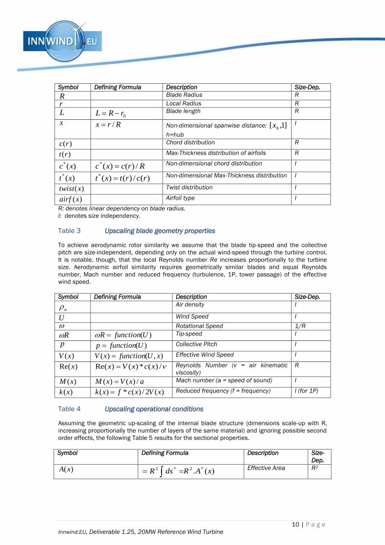
10 | P a g e
Innwind.EU, Deliverable 1.25, 20MW Reference Wind Turbine
Symbol Defining Formula Description Size-Dep.
R Blade Radius R
r Local Radius R
L 0rRL Blade length R
x Rrx / Non-dimensional spanwise distance: ]1,[ hx
h=hub
I
)(rc Chord distribution R
)(rt Max-Thickness distribution of airfoils R
)(* xc Rrcxc /)()(* Non-dimensional chord distribution I
)(* xt )(/)()(* rcrtxt Non-dimensional Max-Thickness distribution I
)(xtwist Twist distribution I
)(xairf Airfoil type I
R: denotes linear dependency on blade radius.
I: denotes size independency.
Table 3 Upscaling blade geometry properties
To achieve aerodynamic rotor similarity we assume that the blade tip-speed and the collective
pitch are size-independent, depending only on the actual wind-speed through the turbine control.
It is notable, though, that the local Reynolds number Re increases proportionally to the turbine
size. Aerodynamic airfoil similarity requires geometrically similar blades and equal Reynolds
number, Mach number and reduced frequency (turbulence, 1P, tower passage) of the effective
wind speed.
Symbol Defining Formula Description Size-Dep.
a Air density I
U Wind Speed I
Rotational Speed 1/R
R )(UfunctionR Tip-speed I
p )(Ufunctionp Collective Pitch I
)(xV ),()( xUfunctionxV Effective Wind Speed I
)Re(x /)(*)()Re( xcxVx Reynolds Number (ν = air kinematic
viscosity)
R
)(xM axVxM /)()( Mach number (a = speed of sound) I
)(xk )(2/)(*)( xVxcfxk Reduced frequency (f = frequency) I (for 1P)
Table 4 Upscaling operational conditions
Assuming the geometric up-scaling of the internal blade structure (dimensions scale-up with R,
increasing proportionally the number of layers of the same material) and ignoring possible second
order effects, the following Table 5 results for the sectional properties.
Symbol Defining Formula Description Size-
Dep.
)(xA )(. *2*2 xARdsR Effective Area R2
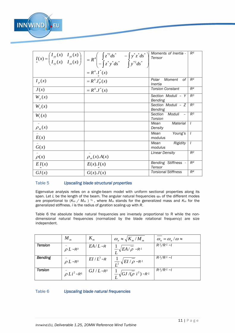
11 | P a g e
Innwind.EU, Deliverable 1.25, 20MW Reference Wind Turbine
)()(
)()()(
xIxI
xIxIxI
zzzy
yzyy
*2****
****2*
4
dsydsyz
dszydszR
)(.*4 xIR
Moments of Inertia -
Tensor
R4
)(xI p )(. *4 xIR P Polar Moment of
Inertia
R4
)(xJ )(. *4 xJR Torsion Constant R4
)(xW y Section Moduli – Y
Bending
R3
)(xWz Section Moduli – Z
Bending
R3
)(xWt Section Moduli –
Torsion
R3
)(xm
Mean Material
Density
I
)(xE
Mean Young’s
modulus
I
)(xG
Mean Rigidity
modulus
I
)(x
)().( xAxm
Linear Density R2
)(xIE
)().( xIxE
Bending Stiffness -
Tensor
R4
)(xGJ )().( xJxG Torsional Stiffness R4
Table 5 Upscaling blade structural properties
Eigenvalue analysis relies on a single-beam model with uniform sectional properties along its
span. Let L be the length of the beam. The angular natural frequencies ωn of the different modes
are proportional to (Km / Mm ) ½ , where Mm stands for the generalized mass and Km for the
generalized stiffness. i is the radius of gyration scaling-up with R.
Table 6 the absolute blade natural frequencies are inversely proportional to R while the non-
dimensional natural frequencies (normalized by the blade rotational frequency) are size
independent.
mM mK
mmn MK / /nn
Tension L
~R3 LEA / ~R
/1
EAL
~R-1 R-1/R-1 ~I
Bending L
~R3
3/ LEI ~R /
12
EIL
~R-1 R-1/R-1 ~I
Torsion 2iL
~R5 LGJ / ~R3
)/(1 2iGJL
~R-1 R-1/R-1 ~I
Table 6 Upscaling blade natural frequencies
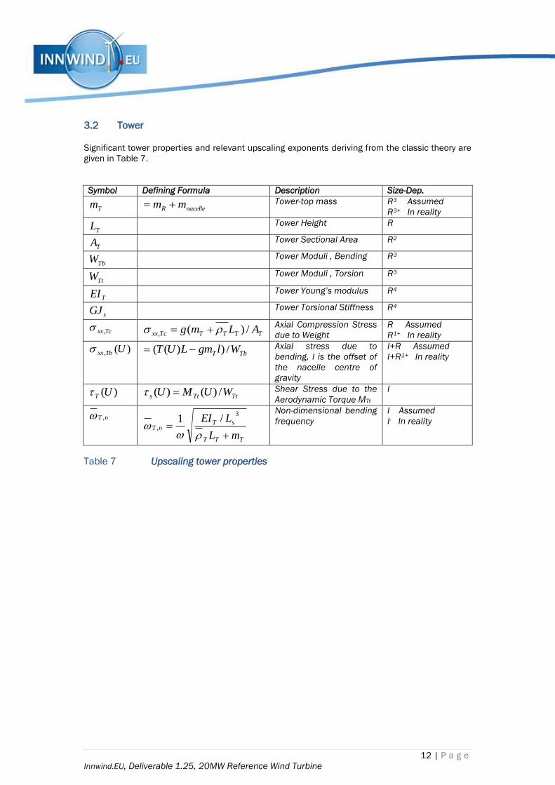
12 | P a g e
Innwind.EU, Deliverable 1.25, 20MW Reference Wind Turbine
3.2 Tower
Significant tower properties and relevant upscaling exponents deriving from the classic theory are
given in Table 7.
Symbol Defining Formula Description Size-Dep.
Tm nacelleR mm Tower-top mass R3 Assumed
R3+ In reality
TL Tower Height R
TA Tower Sectional Area R2
TbW Tower Moduli , Bending R3
TtW Tower Moduli , Torsion R3
TEI Tower Young’s modulus R4
sGJ Tower Torsional Stiffness R4
Tcxx, TTTTTcxx ALmg /)(,
Axial Compression Stress
due to Weight
R Assumed
R1+ In reality
)(, UTbxx TbT WlgmLUT /))(( Axial stress due to
bending, l is the offset of
the nacelle centre of
gravity
I+R Assumed
I+R1+ In reality
)(UT TtTts WUMU /)()( Shear Stress due to the
Aerodynamic Torque MTt
I
nT ,
TTT
sTnT
mL
LEI
3
,
/1
Non-dimensional bending
frequency
I Assumed
I- In reality
Table 7 Upscaling tower properties
13 | P a g e
Innwind.EU, Deliverable 1.25, 20MW Reference Wind Turbine
DEVIATING FROM CLASSICAL UPSCALING
4.1 Rotor
Classical upscaling with cubic scaling factor for the mass is applied for the definition of the 20MW
blades starting from the 10MW ones. The 10MW RWT all-glass blade is a state of the art design
and it is difficult, therefore, to assume a lower scaling factor that could improve the 20MW mass
and cost. The 20MW blade could be designed lighter if a proper integrated design approach was
followed taking advantage of the lower turbulence sub-class (IC) that the design aims for.
Nevertheless, the classically up-scaled 20MW blade is a good starting point to serve as a
reference in the present context. No deviations from the classical theory are assumed here.
4.2 Nacelle – Hub
We take advantage of the lower turbine subclass to assume less than cubic mass scaling factors
for the hub and the nacelle. For the nacelle we assume that its weight can be further reduced
through technological interventions that maintain the current learning curve trends. The following
values are used:
Hub : SF = 2.8 Mass = 278 t
Nacelle : SF = 2.6 Mass = 1 098 t
4.3 Drive train
The drive train weight is part of the nacelle weight discussed above. Drive train deviations from
classical upscaling address the 5% increase of the rated rotor speed which now becomes 7.13
RPM. We further assume that we maintain the medium speed drive of the 10MW RWT with
Rated Generator Speed: SF = -1.0 N = 339 RPM
yielding a Gearing Ratio of 48. No further deviations from classical theory are anticipated.
4.4 Tower
Significant deviation from the classical upscaling theory is normally encountered in offshore wind
turbine design. The usual choice, which accounts the fact that the wind shear exponent is lower
offshore than onshore (at least for flat terrain) and thus a longer tower is less cost effective, is that
the tower height is not up-scaled with SF = 1 but in a way that maintains the blade water
clearance to a prescribed level. In this case the new tower may derive by first up-scaling linearly
the reference tower and then cutting its bottom part as much as needed to match the desired hub
height.
The above described approach was also the starting point for designing the land version of the
20MW tower. The first global system frequency calculated in this case was 0.208 Hz (5th row of
Table 8, corresponding to the SFs presented above for the RNA components). This is a rather high
starting value which would further increase to 0.231 Hz if the lower 20m of the tower was made
extra stiff, resembling the influence of the jacket (6th row of Table 8, “stiff” version).
To appreciate the influence of the tower design parameters on the 1st system frequency we
performed several calculations assuming a tower / top-mass system and changing in a global way
along the height the tower radius, thickness and height as depicted in Table 8. In the Table we
present the 1st system frequency which derives from different combinations of the blades/ hub/
nacelle weight scaling factors, tower radius and wall thickness global multipliers and tower height.

14 | P a g e
Innwind.EU, Deliverable 1.25, 20MW Reference Wind Turbine
In most of the cases we consider a “soft” and a “stiff” option, the later as defined in an earlier
paragraph. The study showed that making the tower softer needs excessive extra mass (lowering
the radius and increasing the wall thickness to maintain the level of bending resistance) if the
tower height is not increased. As a more efficient way to soften the system frequency it was
chosen to increase the tower height (we selected a value of 12m).
Table 8 Alternative tower designs and their effect on 1st global frequency
The baseline frequency of the longer tower “soft” (normal) version, hereafter called Tower 2, is
0.193 Hz which would increase to 0,208 Hz for the “stiff” version (Tower 1). In this case the
stiffening is materialized by increasing artificially the rigidity of the first 15 meters of Tower 2. If
the wall thickness of the tower might reduce by 10%, thanks to the lower ultimate fatigue and
buckling loading of the selected IC turbine class, the baseline frequency would further reduce to
0.184 Hz (Tower 3). These three tower options are selected as alternatives for tower base load
calculations communicated to WP4 for designing the 20MW jacket.
4.5 Control
Similar upscaling techniques have been used for the Standard DTU Controller parameters on the
basis of their values for the 10MW RWT. The 5% over-speed is also taken into account. The full
list of the controller parameters for the 20MW RWT is given in Appendix I. In red fond we present
deviations from classical upscaling. Note that no exclusion zone is present but we compromise
optimal variable speed generation by initiating at 7m/s wind speed corresponding to a minimum
rotor speed of 0.45 rad/s. The value of “Constant 11” addressing the optimal Cp tracking factor
SF. Blade
Weight
SF.Hub
Weight
SF.Nacell
e Weight
Tower
Radius *
Tower
Thickn *
Tower
Height
(+ m)
1st
SYSTEM
FREQ (Hz)
Soft /
Stiff
3.00 3.00 3.00 1.00 1.00 0.00 0.199 soft
3.00 3.00 3.00 1.00 1.00 0.00 0.221 stiff
3.00 3.00 3.00 0.80 1.56 0.00 0.195 soft
3.00 3.00 3.00 0.80 1.56 0.00 0.218 stiff
3.00 2.80 2.60 1.00 1.00 0.00 0.208 soft
3.00 2.80 2.60 1.00 1.00 0.00 0.231 stiff
3.00 2.80 2.60 0.80 1.56 0.00 0.205 soft
3.00 2.80 2.60 0.80 1.56 0.00 0.228 stiff
3.00 2.80 2.60 1.00 0.90 0.00 0.198 soft
3.00 2.80 2.60 1.00 0.80 0.00 0.188 soft
3.00 2.80 2.60 1.00 1.00 0.00 0.208 soft
3.00 2.80 2.60 1.00 1.00 0.00 0.231 stiff
3.00 2.80 2.60 1.00 1.00 10.00 0.195 soft
3.00 2.80 2.60 1.00 1.00 10.00 0.215 stiff
3.00 2.80 2.60 1.00 1.00 12.00 0.208 stiff
3.00 2.80 2.60 1.00 1.00 12.00 0.193 soft
3.00 2.80 2.60 1.00 0.90 12.00 0.184 soft
3.00 2.80 2.60 1.00 1.00 20.00 0.183 soft
3.00 2.80 2.60 1.00 1.00 20.00 0.205 stiff

15 | P a g e
Innwind.EU, Deliverable 1.25, 20MW Reference Wind Turbine
has been calculated explicitly using the exact values of its defining formula, taking into account
the 5% rotor over-speed.
4.6 Design summary
Table 9 presents the design summary of the 20MW Reference Wind Turbine deriving from the
above assumptions. Contrary to other properties the tower weight of the land version is given as a
range of values from 1600 to 1780 tonnes corresponding to the two alternative “soft” designs
discussed above.
Table 9 Design summary of the 20 MW RWT vs the 10 MW RWT
Rated Power [MW] 10 20
Number of blades [-] 3 3
Rotor Diameter [m] 178.33 252.2
Hub Height from m.s.l. [m] 119 167.9
Blade Length [m] 86.36 122.14
Rated Wind Speed [m/s] 11.4 11.4
Design Extreme Thrust Value [kN] 4600 9600
Minimum Rotor Speed [RPM] 6 4.45
Rated Rotor Speed [RPM] 9.6 7.13
Optimal TSR [-] 7.5 7.5
Gear Ratio [-] 50 48
Blade Mass [tons] 41.7 118
Hub Mass [tons] 105.5 278
Nacelle mass [tons] 446 1098
Tower mass [tons] 628.4 1600-1780
Tower Top Mass, RNA [tons] 676.7 1730
Water depth (mean sea level - m.s.l.) [m] 50 50
Access Platform a.m.s.l. [m] 25 25
Jacket Mass [Tons] 1210 -
Transition piece mass [Tons] 330 -
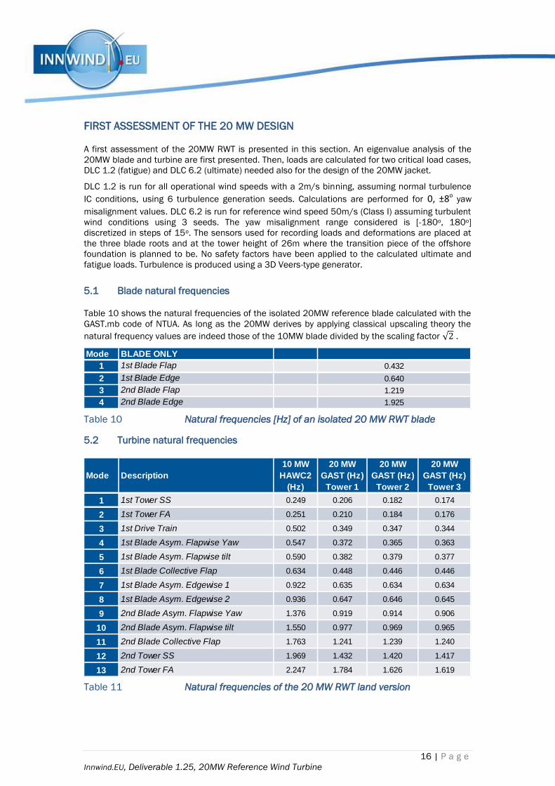
16 | P a g e
Innwind.EU, Deliverable 1.25, 20MW Reference Wind Turbine
FIRST ASSESSMENT OF THE 20 MW DESIGN
A first assessment of the 20MW RWT is presented in this section. An eigenvalue analysis of the
20MW blade and turbine are first presented. Then, loads are calculated for two critical load cases,
DLC 1.2 (fatigue) and DLC 6.2 (ultimate) needed also for the design of the 20MW jacket.
DLC 1.2 is run for all operational wind speeds with a 2m/s binning, assuming normal turbulence
IC conditions, using 6 turbulence generation seeds. Calculations are performed for 0, ±8o yaw
misalignment values. DLC 6.2 is run for reference wind speed 50m/s (Class I) assuming turbulent
wind conditions using 3 seeds. The yaw misalignment range considered is [-180o, 180o]
discretized in steps of 15o. The sensors used for recording loads and deformations are placed at
the three blade roots and at the tower height of 26m where the transition piece of the offshore
foundation is planned to be. No safety factors have been applied to the calculated ultimate and
fatigue loads. Turbulence is produced using a 3D Veers-type generator.
5.1 Blade natural frequencies
Table 10 shows the natural frequencies of the isolated 20MW reference blade calculated with the
GAST.mb code of NTUA. As long as the 20MW derives by applying classical upscaling theory the
natural frequency values are indeed those of the 10MW blade divided by the scaling factor √2 .
Table 10 Natural frequencies [Hz] of an isolated 20 MW RWT blade
5.2 Turbine natural frequencies
Table 11 Natural frequencies of the 20 MW RWT land version
Mode BLADE ONLY
1 1st Blade Flap
2 1st Blade Edge
3 2nd Blade Flap
4 2nd Blade Edge
0.432
0.640
1.219
1.925
Mode Description
10 MW
HAWC2
(Hz)
20 MW
GAST (Hz)
Tower 1
20 MW
GAST (Hz)
Tower 2
20 MW
GAST (Hz)
Tower 3
1 1st Tower SS 0.249 0.206 0.182 0.174
2 1st Tower FA 0.251 0.210 0.184 0.176
3 1st Drive Train 0.502 0.349 0.347 0.344
4 1st Blade Asym. Flapwise Yaw 0.547 0.372 0.365 0.363
5 1st Blade Asym. Flapwise tilt 0.590 0.382 0.379 0.377
6 1st Blade Collective Flap 0.634 0.448 0.446 0.446
7 1st Blade Asym. Edgewise 1 0.922 0.635 0.634 0.634
8 1st Blade Asym. Edgewise 2 0.936 0.647 0.646 0.645
9 2nd Blade Asym. Flapwise Yaw 1.376 0.919 0.914 0.906
10 2nd Blade Asym. Flapwise tilt 1.550 0.977 0.969 0.965
11 2nd Blade Collective Flap 1.763 1.241 1.239 1.240
12 2nd Tower SS 1.969 1.432 1.420 1.417
13 2nd Tower FA 2.247 1.784 1.626 1.619
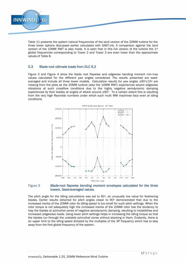
17 | P a g e
Innwind.EU, Deliverable 1.25, 20MW Reference Wind Turbine
Table 11 presents the system natural frequencies of the land version of the 20MW turbine for the
three tower options discussed earlier calculated with GAST.mb. A comparison against the land
version of the 10MW RWT is also made. It is seen that in this full version of the turbine the 1st
global frequencies corresponding to Tower 2 and Tower 3 are even lower than the approximate
values of Table 8.
5.3 Blade root ultimate loads from DLC 6.2
Figure 3 and Figure 4 show the blade root flapwise and edgewise bending moment min-max
values calculated for the different yaw angles considered. The results presented are seed-
averaged and include all three tower models. Calculation results for yaw angles ±90o±15o are
missing from the plots as the 20MW turbine (also the 10MW RWT) experiences severe edgewise
vibrations at such crossflow conditions due to the highly negative aerodynamic damping
experienced by their blades at angles of attack around ±90o. To a certain extent this is resulting
from the very high Reynolds numbers under which such multi MW machines face even at idling
conditions.
Figure 3 Blade-root flapwise bending moment envelopes calculated for the three
towers. Seed-averaged values.
The pitch angle for the idling calculations was set to 82o, an unusually low value for feathering
blades. Earlier results obtained for pitch angles closer to 90o demonstrated that due to the
increased inertia of the 20MW rotor its idling speed is too small for such pitch settings. When the
rotor torque is not adequately high the increased inertia of the 20MW rotor has the tendency to
trap the blades at azimuthal zones of negative aerodynamic damping, resulting to instabilities and
increased (edgewise) loads. Using lower pitch settings helps in increasing the idling torque so that
the blades run through the unstable azimuthal zones without stacking in them. Evidently, there is
an upper limit to the idling speed dictated by the multiples of the 3P frequency which has to stay
away from the first global frequency of the system.
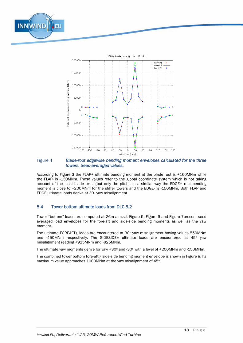
18 | P a g e
Innwind.EU, Deliverable 1.25, 20MW Reference Wind Turbine
Figure 4 Blade-root edgewise bending moment envelopes calculated for the three
towers. Seed-averaged values.
According to Figure 3 the FLAP+ ultimate bending moment at the blade root is +160MNm while
the FLAP- is -130MNm. These values refer to the global coordinate system which is not taking
account of the local blade twist (but only the pitch). In a similar way the EDGE+ root bending
moment is close to +200MNm for the stiffer towers and the EDGE- is -150MNm. Both FLAP and
EDGE ultimate loads derive at 30o yaw misalignment.
5.4 Tower bottom ultimate loads from DLC 6.2
Tower “bottom” loads are computed at 26m a.m.s.l. Figure 5, Figure 6 and Figure 7present seed
averaged load envelopes for the fore-aft and side-side bending moments as well as the yaw
moment.
The ultimate FOREAFT± loads are encountered at 30o yaw misalignment having values 550MNm
and -450MNm respectively. The SIDESIDE± ultimate loads are encountered at 45o yaw
misalignment reading +925MNm and -825MNm.
The ultimate yaw moments derive for yaw +30o and -30o with a level of +200MNm and -150MNm.
The combined tower bottom fore-aft / side-side bending moment envelope is shown in Figure 8. Its
maximum value approaches 1000MNm at the yaw misalignment of 45o.
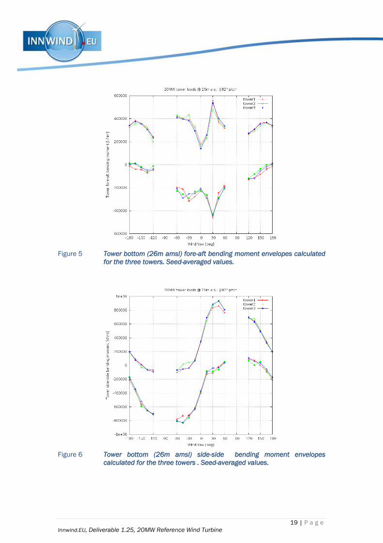
19 | P a g e
Innwind.EU, Deliverable 1.25, 20MW Reference Wind Turbine
Figure 5 Tower bottom (26m amsl) fore-aft bending moment envelopes calculated
for the three towers. Seed-averaged values.
Figure 6 Tower bottom (26m amsl) side-side bending moment envelopes
calculated for the three towers . Seed-averaged values.
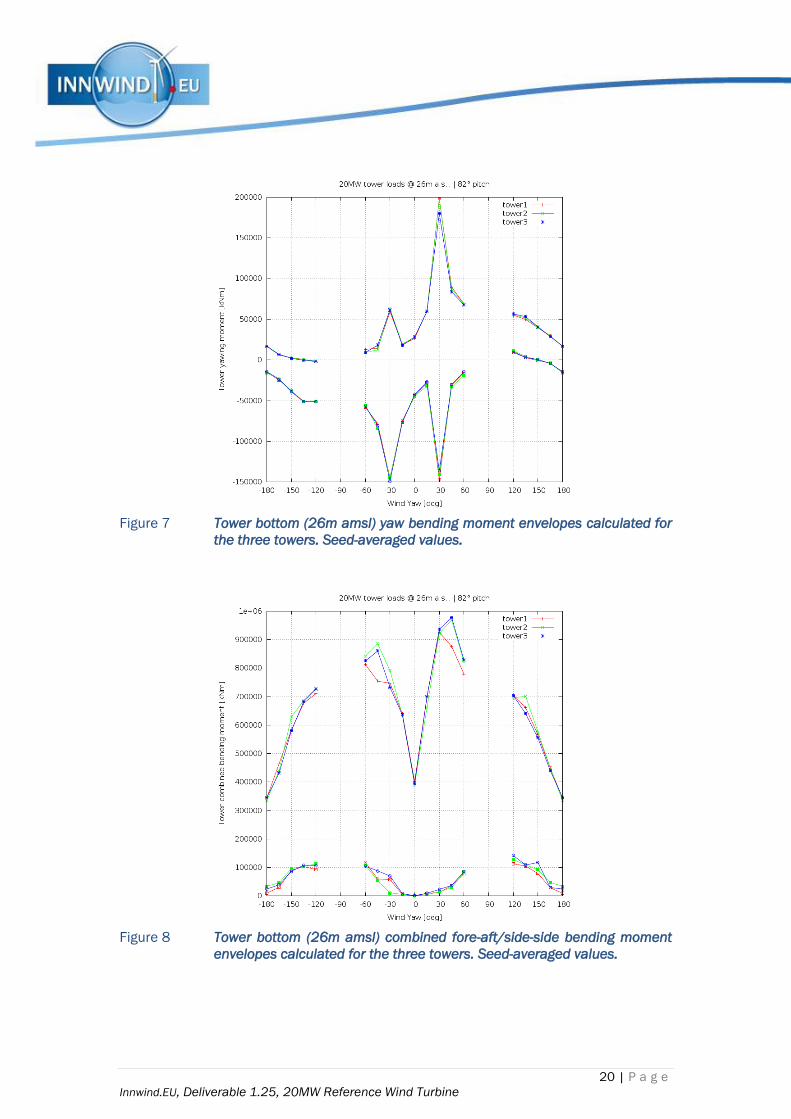
20 | P a g e
Innwind.EU, Deliverable 1.25, 20MW Reference Wind Turbine
Figure 7 Tower bottom (26m amsl) yaw bending moment envelopes calculated for
the three towers. Seed-averaged values.
Figure 8 Tower bottom (26m amsl) combined fore-aft/side-side bending moment
envelopes calculated for the three towers. Seed-averaged values.

21 | P a g e
Innwind.EU, Deliverable 1.25, 20MW Reference Wind Turbine
5.5 Blade root fatigue loads from DLC 1.2
Characteristic values of blade root flapwise and edgewise moments calculated for Tower 1 for zero
yaw as a function of the wind speed for all 6 turbulent seeds are presented in Figure 9 and Figure
10 respectively. The figure presents min-max values per seed (the coloured bars), mean value per
wind speed for all seeds (continuous black line) and standard deviation mean for all seeds
(continuous white line). The same notation and colouring scheme is used in all fatigue load plots.
In the present context we present blade toot results for Tower 1 and for the zero yaw angle. The
full set of results, for all three towers and all three yaw angles are included in Appendix II. The
influence of the yaw misalignment and the tower selection on blade root fatigue loads is rather
small.
Figure 9 Blade-root flapwise bending moments for Tower 1 and yaw angles 0 for
all wind speeds and turbulent seeds
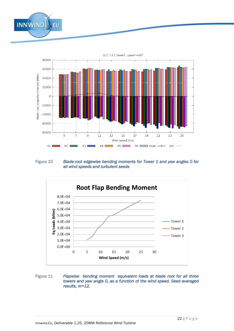
22 | P a g e
Innwind.EU, Deliverable 1.25, 20MW Reference Wind Turbine
Figure 10 Blade-root edgewise bending moments for Tower 1 and yaw angles 0 for
all wind speeds and turbulent seeds
Figure 11 Flapwise bending moment equivalent loads at blade root for all three
towers and yaw angle 0, as a function of the wind speed. Seed averaged
results, m=12.
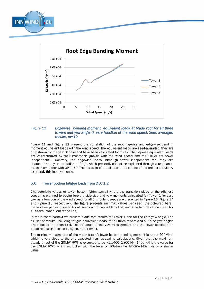
23 | P a g e
Innwind.EU, Deliverable 1.25, 20MW Reference Wind Turbine
Figure 12 Edgewise bending moment equivalent loads at blade root for all three
towers and yaw angle 0, as a function of the wind speed. Seed averaged
results, m=12.
Figure 11 and Figure 12 present the correlation of the root flapwise and edgewise bending
moment equivalent loads with the wind speed. The equivalent loads are seed-averaged, they are
only shown for the yaw 0o case and have been calculated for m=12. The flapwise equivalent loads
are characterized by their monotonic growth with the wind speed and their level are tower
independent. Contrary, the edgewise loads, although tower independent too, they are
characterized by an excitation at 9m/s which presently cannot be explained through a resonance
mechanism either with 3P or 6P. The redesign of the blades in the course of the project should try
to remedy this inconvenience.
5.6 Tower bottom fatigue loads from DLC 1.2
Characteristic values of tower bottom (26m a.m.s.l where the transition piece of the offshore
version is planned to begin) fore-aft, side-side and yaw moments calculated for Tower 1 for zero
yaw as a function of the wind speed for all 6 turbulent seeds are presented in Figure 13, Figure 14
and Figure 15 respectively. The figure presents min-max values per seed (the coloured bars),
mean value per wind speed for all seeds (continuous black line) and standard deviation mean for
all seeds (continuous white line).
In the present context we present blade toot results for Tower 1 and for the zero yaw angle. The
full set of results, including fatigue equivalent loads, for all three towers and all three yaw angles
are included in Appendix II. The influence of the yaw misalignment and the tower selection on
blade root fatigue loads is, again, rather small.
The maximum magnitude of the mean fore-aft tower bottom bending moment is about 400MNm
which is very close to the one expected from up-scaling calculations. Given that the maximum
steady thrust of the 20MW RWT is expected to be ~2.1400=2800 kN (1400 kN is the value for
the 10MW RWT) which multiplied with the lever of 168(hub height)-26=142m yields a similar
value.
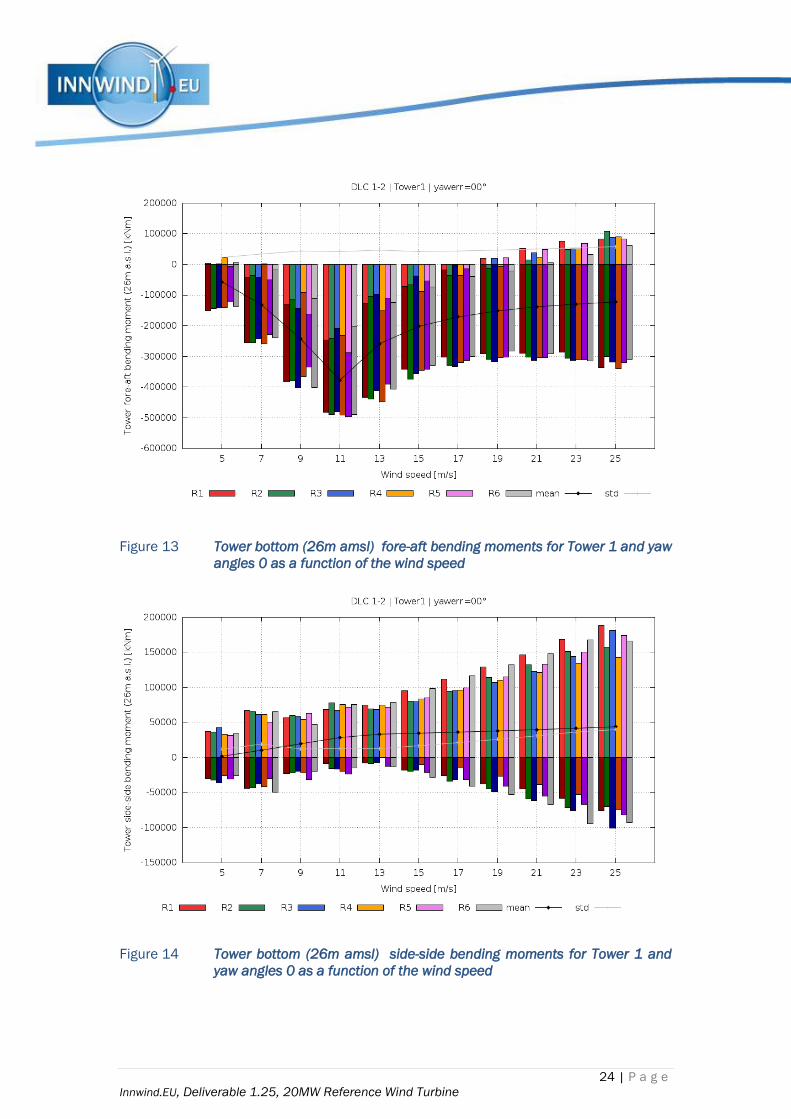
24 | P a g e
Innwind.EU, Deliverable 1.25, 20MW Reference Wind Turbine
Figure 13 Tower bottom (26m amsl) fore-aft bending moments for Tower 1 and yaw
angles 0 as a function of the wind speed
Figure 14 Tower bottom (26m amsl) side-side bending moments for Tower 1 and
yaw angles 0 as a function of the wind speed
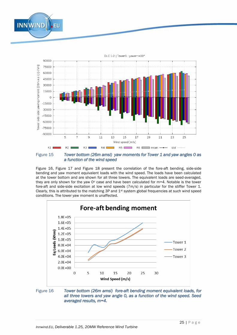
25 | P a g e
Innwind.EU, Deliverable 1.25, 20MW Reference Wind Turbine
Figure 15 Tower bottom (26m amsl) yaw moments for Tower 1 and yaw angles 0 as
a function of the wind speed
Figure 16, Figure 17 and Figure 18 present the correlation of the fore-aft bending, side-side
bending and yaw moment equivalent loads with the wind speed. The loads have been calculated
at the tower bottom and are shown for all three towers. The equivalent loads are seed-averaged,
they are only shown for the yaw 0o case and have been calculated for m=4. Notable is the tower
fore-aft and side-side excitation at low wind speeds (7m/s) in particular for the stiffer Tower 1.
Clearly, this is attributed to the matching 3P and 1st system global frequencies at such wind speed
conditions. The tower yaw moment is unaffected.
Figure 16 Tower bottom (26m amsl) fore-aft bending moment equivalent loads, for
all three towers and yaw angle 0, as a function of the wind speed. Seed
averaged results, m=4.
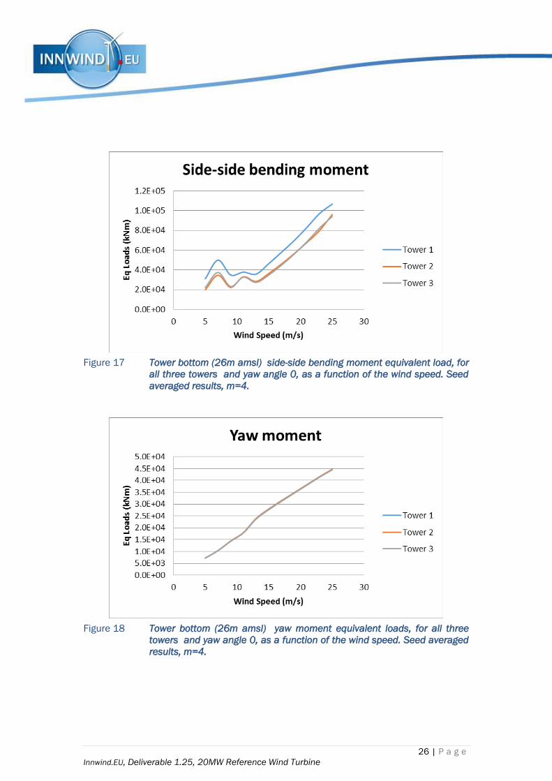
26 | P a g e
Innwind.EU, Deliverable 1.25, 20MW Reference Wind Turbine
Figure 17 Tower bottom (26m amsl) side-side bending moment equivalent load, for
all three towers and yaw angle 0, as a function of the wind speed. Seed
averaged results, m=4.
Figure 18 Tower bottom (26m amsl) yaw moment equivalent loads, for all three
towers and yaw angle 0, as a function of the wind speed. Seed averaged
results, m=4.

27 | P a g e
Innwind.EU, Deliverable 1.25, 20MW Reference Wind Turbine
SUMMARY
In this document we presented the design and a preliminary evaluation of the land version of the
20 MW Reference Wind Turbine of INNWIND.EU project.
The 20MW RWT derived from the upscaling of the 10MW DTU RWT and is intended to be a Class
IC. Classical upscaling techniques were the starting point for configuring all 20MW turbine
subsystems. In a second step the up-scaled data were adjusted to include learning curve
expectations in terms for components mases and to face particular challenges regarding the
proper selection of the first systems’ frequency in connection to the variable speed schedule of
the turbine.
The design summary of the turbine is compared against that of the 10MW RWT. The aeroelastic
data of the turbine and its subcomponents are given in XLS spreadsheets that accompany this
report.
System natural frequencies and loads are calculated for the 20MW RWT. Blade and tower root
ultimate and fatigue loads are presented for two relevant IEC-61400 design load cases, D6.2 for
ultimate and D1.2 for fatigue loads. The tower bottom loads extracted are delivered to WP4 for the
design of the 20MW reference jacket.

28 | P a g e
Innwind.EU, Deliverable 1.25, 20MW Reference Wind Turbine
REFERENCES
1. Berger F. et al. System design assessment for innovative support structures. INNWIND.EU
D1.35, October 2015.
2. Chaviaropoulos PK. Similarity rules for W/T up-scaling. UPWIND Report, WP 1B4, 2007.
3. Sieros G, Chaviaropoulos P, Sorensen JD, Bulder BH, Jamieson P. Up-scaling Wind
Turbines: Theoretical and practical aspects and their impact on the cost of energy. Wind
Energy 2012. 15(1): 3-17.
4. Sieros G, Chaviaropoulos P.K. Aspects of up-scaling beyond similarity. Proceedings of ‘The
Science of Making Torque from Wind’ Conference, Heraklion, Greece, 28-30/6/2010,
Edited by S. Voutsinas and P. K. Chaviaropoulos.
5. Wind Turbine Design Cost and Scaling Model, by L. Fingersh, M. Hand, and A. Laxson,
NREL/TP-500-40566, December 2006.
6. Chaviaropoulos, T, H.J.M. Beurskens and S. Voutsinas, Moving towards large(r) high speed
rotors – is that a good idea? Proc. Scientific Track, EWEA 2013 Conference, Vienna.
7. Key Performance Indicators for the European Wind Industrial Initiative, SETIS-TPWIND,
Version: 3, 7th November 2011.
8. Peter Jamieson, Innovation in Wind Turbine Design, A John Wiley & Sons, Ltd., Publication,
ISBN 978-0-470-69981-2, 2011.
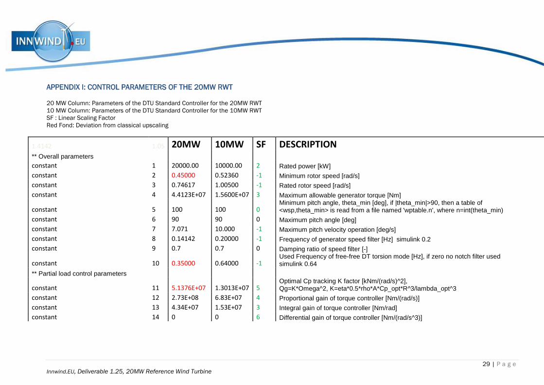
29 | P a g e
Innwind.EU, Deliverable 1.25, 20MW Reference Wind Turbine
APPENDIX I: CONTROL PARAMETERS OF THE 20MW RWT
20 MW Column: Parameters of the DTU Standard Controller for the 20MW RWT
10 MW Column: Parameters of the DTU Standard Controller for the 10MW RWT
SF : Linear Scaling Factor
Red Fond: Deviation from classical upscaling
1.4142 1.05 20MW 10MW SF DESCRIPTION ** Overall parameters
constant 1 20000.00 10000.00 2 Rated power [kW]
constant 2 0.45000 0.52360 -1 Minimum rotor speed [rad/s]
constant 3 0.74617 1.00500 -1 Rated rotor speed [rad/s]
constant 4 4.4123E+07 1.5600E+07 3 Maximum allowable generator torque [Nm]
constant 5 100 100 0 Minimum pitch angle, theta_min [deg], if |theta_min|>90, then a table of <wsp,theta_min> is read from a file named 'wptable.n', where n=int(theta_min)
constant 6 90 90 0 Maximum pitch angle [deg]
constant 7 7.071 10.000 -1 Maximum pitch velocity operation [deg/s]
constant 8 0.14142 0.20000 -1 Frequency of generator speed filter [Hz] simulink 0.2
constant 9 0.7 0.7 0 Damping ratio of speed filter [-]
constant 10 0.35000 0.64000 -1 Used Frequency of free-free DT torsion mode [Hz], if zero no notch filter used simulink 0.64
** Partial load control parameters
constant 11 5.1376E+07 1.3013E+07 5 Optimal Cp tracking K factor [kNm/(rad/s)^2], Qg=K*Omega^2, K=eta*0.5*rho*A*Cp_opt*R^3/lambda_opt^3
constant 12 2.73E+08 6.83E+07 4 Proportional gain of torque controller [Nm/(rad/s)]
constant 13 4.34E+07 1.53E+07 3 Integral gain of torque controller [Nm/rad]
constant 14 0 0 6 Differential gain of torque controller [Nm/(rad/s^3)]
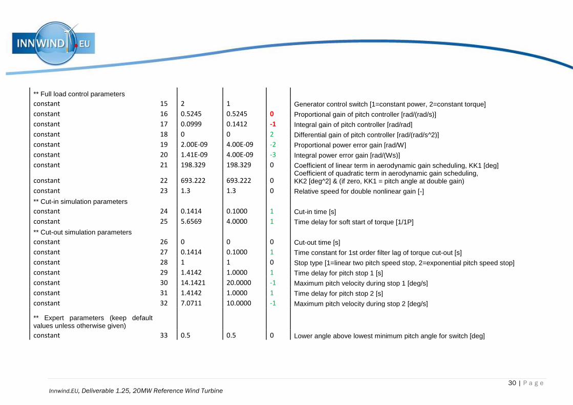
30 | P a g e
Innwind.EU, Deliverable 1.25, 20MW Reference Wind Turbine
** Full load control parameters
constant 15 2 1 Generator control switch [1=constant power, 2=constant torque]
constant 16 0.5245 0.5245 0 Proportional gain of pitch controller [rad/(rad/s)]
constant 17 0.0999 0.1412 -1 Integral gain of pitch controller [rad/rad]
constant 18 0 0 2 Differential gain of pitch controller [rad/(rad/s^2)]
constant 19 2.00E-09 4.00E-09 -2 Proportional power error gain [rad/W]
constant 20 1.41E-09 4.00E-09 -3 Integral power error gain [rad/(Ws)]
constant 21 198.329 198.329 0 Coefficient of linear term in aerodynamic gain scheduling, KK1 [deg]
constant 22 693.222 693.222 0 Coefficient of quadratic term in aerodynamic gain scheduling, KK2 [deg^2] & (if zero, KK1 = pitch angle at double gain)
constant 23 1.3 1.3 0 Relative speed for double nonlinear gain [-]
** Cut-in simulation parameters
constant 24 0.1414 0.1000 1 Cut-in time [s]
constant 25 5.6569 4.0000 1 Time delay for soft start of torque [1/1P]
** Cut-out simulation parameters
constant 26 0 0 0 Cut-out time [s]
constant 27 0.1414 0.1000 1 Time constant for 1st order filter lag of torque cut-out [s]
constant 28 1 1 0 Stop type [1=linear two pitch speed stop, 2=exponential pitch speed stop]
constant 29 1.4142 1.0000 1 Time delay for pitch stop 1 [s]
constant 30 14.1421 20.0000 -1 Maximum pitch velocity during stop 1 [deg/s]
constant 31 1.4142 1.0000 1 Time delay for pitch stop 2 [s]
constant 32 7.0711 10.0000 -1 Maximum pitch velocity during stop 2 [deg/s]
** Expert parameters (keep default values unless otherwise given)
constant 33 0.5 0.5 0 Lower angle above lowest minimum pitch angle for switch [deg]
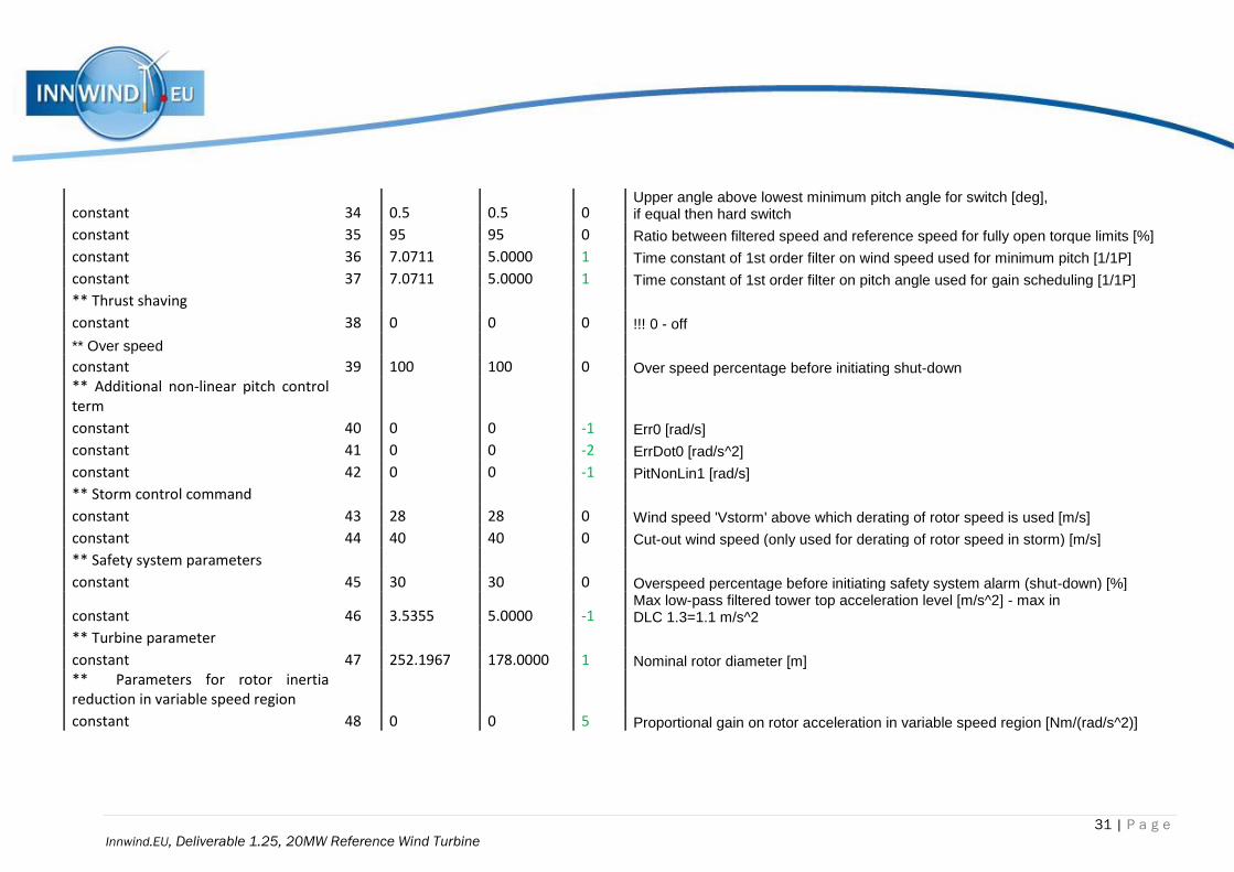
31 | P a g e
Innwind.EU, Deliverable 1.25, 20MW Reference Wind Turbine
constant 34 0.5 0.5 0 Upper angle above lowest minimum pitch angle for switch [deg], if equal then hard switch
constant 35 95 95 0 Ratio between filtered speed and reference speed for fully open torque limits [%]
constant 36 7.0711 5.0000 1 Time constant of 1st order filter on wind speed used for minimum pitch [1/1P]
constant 37 7.0711 5.0000 1 Time constant of 1st order filter on pitch angle used for gain scheduling [1/1P]
** Thrust shaving
constant 38 0 0 0 !!! 0 - off
** Over speed
constant 39 100 100 0 Over speed percentage before initiating shut-down
** Additional non-linear pitch control term
constant 40 0 0 -1 Err0 [rad/s]
constant 41 0 0 -2 ErrDot0 [rad/s^2]
constant 42 0 0 -1 PitNonLin1 [rad/s]
** Storm control command
constant 43 28 28 0 Wind speed 'Vstorm' above which derating of rotor speed is used [m/s]
constant 44 40 40 0 Cut-out wind speed (only used for derating of rotor speed in storm) [m/s]
** Safety system parameters
constant 45 30 30 0 Overspeed percentage before initiating safety system alarm (shut-down) [%]
constant 46 3.5355 5.0000 -1 Max low-pass filtered tower top acceleration level [m/s^2] - max in DLC 1.3=1.1 m/s^2
** Turbine parameter
constant 47 252.1967 178.0000 1 Nominal rotor diameter [m]
** Parameters for rotor inertia reduction in variable speed region
constant 48 0 0 5 Proportional gain on rotor acceleration in variable speed region [Nm/(rad/s^2)]
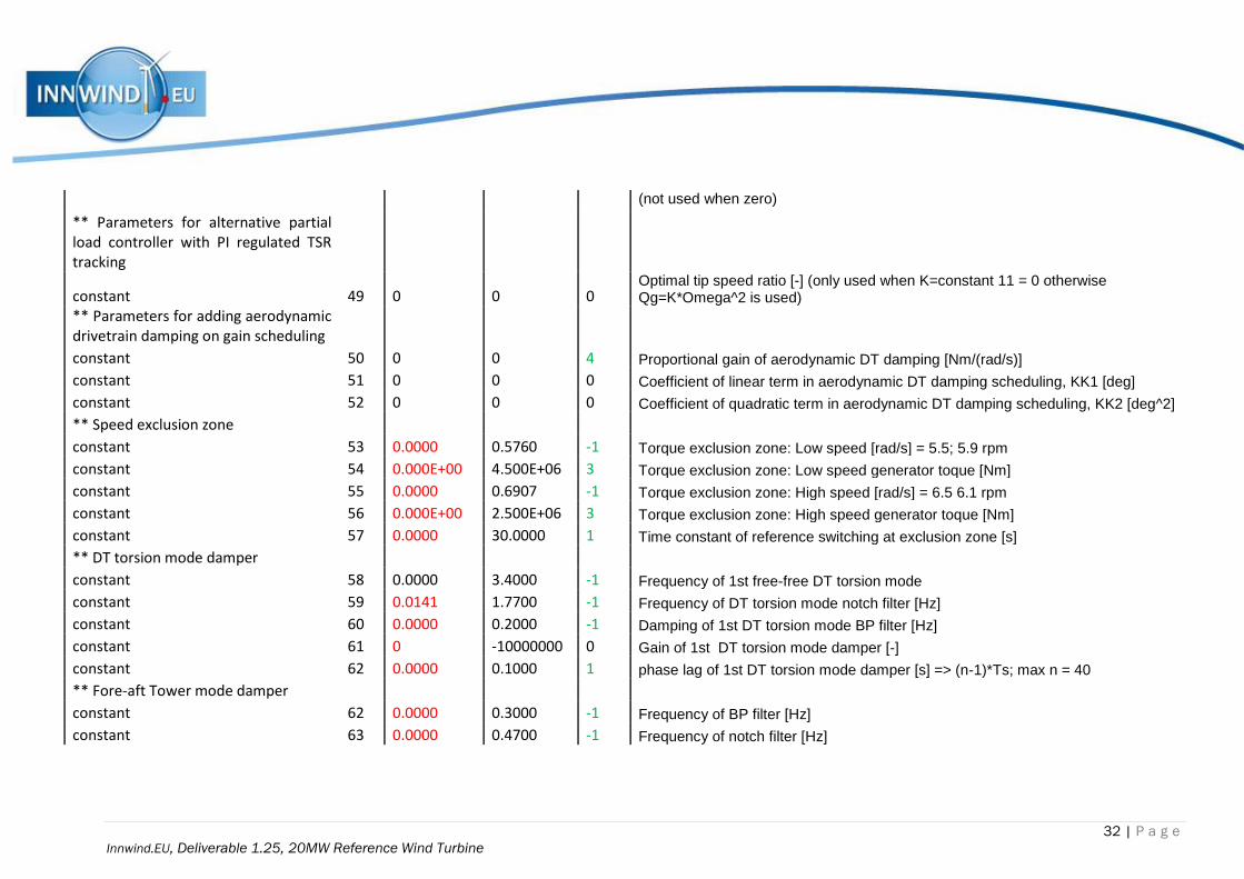
32 | P a g e
Innwind.EU, Deliverable 1.25, 20MW Reference Wind Turbine
(not used when zero)
** Parameters for alternative partial load controller with PI regulated TSR tracking
constant 49 0 0 0 Optimal tip speed ratio [-] (only used when K=constant 11 = 0 otherwise Qg=K*Omega^2 is used)
** Parameters for adding aerodynamic drivetrain damping on gain scheduling
constant 50 0 0 4 Proportional gain of aerodynamic DT damping [Nm/(rad/s)]
constant 51 0 0 0 Coefficient of linear term in aerodynamic DT damping scheduling, KK1 [deg]
constant 52 0 0 0 Coefficient of quadratic term in aerodynamic DT damping scheduling, KK2 [deg^2]
** Speed exclusion zone
constant 53 0.0000 0.5760 -1 Torque exclusion zone: Low speed [rad/s] = 5.5; 5.9 rpm
constant 54 0.000E+00 4.500E+06 3 Torque exclusion zone: Low speed generator toque [Nm]
constant 55 0.0000 0.6907 -1 Torque exclusion zone: High speed [rad/s] = 6.5 6.1 rpm
constant 56 0.000E+00 2.500E+06 3 Torque exclusion zone: High speed generator toque [Nm]
constant 57 0.0000 30.0000 1 Time constant of reference switching at exclusion zone [s]
** DT torsion mode damper
constant 58 0.0000 3.4000 -1 Frequency of 1st free-free DT torsion mode
constant 59 0.0141 1.7700 -1 Frequency of DT torsion mode notch filter [Hz]
constant 60 0.0000 0.2000 -1 Damping of 1st DT torsion mode BP filter [Hz]
constant 61 0 -10000000 0 Gain of 1st DT torsion mode damper [-]
constant 62 0.0000 0.1000 1 phase lag of 1st DT torsion mode damper [s] => (n-1)*Ts; max n = 40
** Fore-aft Tower mode damper
constant 62 0.0000 0.3000 -1 Frequency of BP filter [Hz]
constant 63 0.0000 0.4700 -1 Frequency of notch filter [Hz]
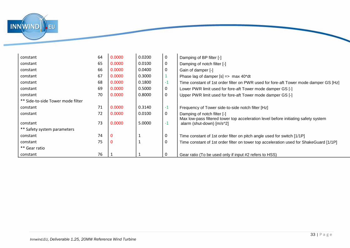
33 | P a g e
Innwind.EU, Deliverable 1.25, 20MW Reference Wind Turbine
constant 64 0.0000 0.0200 0 Damping of BP filter [-]
constant 65 0.0000 0.0100 0 Damping of notch filter [-]
constant 66 0.0000 0.0400 0 Gain of damper [-]
constant 67 0.0000 0.3000 1 Phase lag of damper [s] => max 40*dt
constant 68 0.0000 0.1800 -1 Time constant of 1st order filter on PWR used for fore-aft Tower mode damper GS [Hz]
constant 69 0.0000 0.5000 0 Lower PWR limit used for fore-aft Tower mode damper GS [-]
constant 70 0.0000 0.8000 0 Upper PWR limit used for fore-aft Tower mode damper GS [-]
** Side-to-side Tower mode filter
constant 71 0.0000 0.3140 -1 Frequency of Tower side-to-side notch filter [Hz]
constant 72 0.0000 0.0100 0 Damping of notch filter [-]
constant 73 0.0000 5.0000 -1 Max low-pass filtered tower top acceleration level before initiating safety system alarm (shut-down) [m/s^2]
** Safety system parameters
constant 74 0 1 0 Time constant of 1st order filter on pitch angle used for switch [1/1P]
constant 75 0 1 0 Time constant of 1st order filter on tower top acceleration used for ShakeGuard [1/1P]
** Gear ratio
constant 76 1 1 0 Gear ratio (To be used only if input #2 refers to HSS)

34 | P a g e
Innwind.EU, Deliverable 1.25, 20MW Reference Wind Turbine
APPENDIX IΙ: FATIGUE RESULTS FOR ALL TOWER VERSIONS OF THE 20MW RWT
Figure 19 Blade-root flapwise bending moments for Tower 1 and yaw angles 0 and
±8 degrees as a function of the wind speed
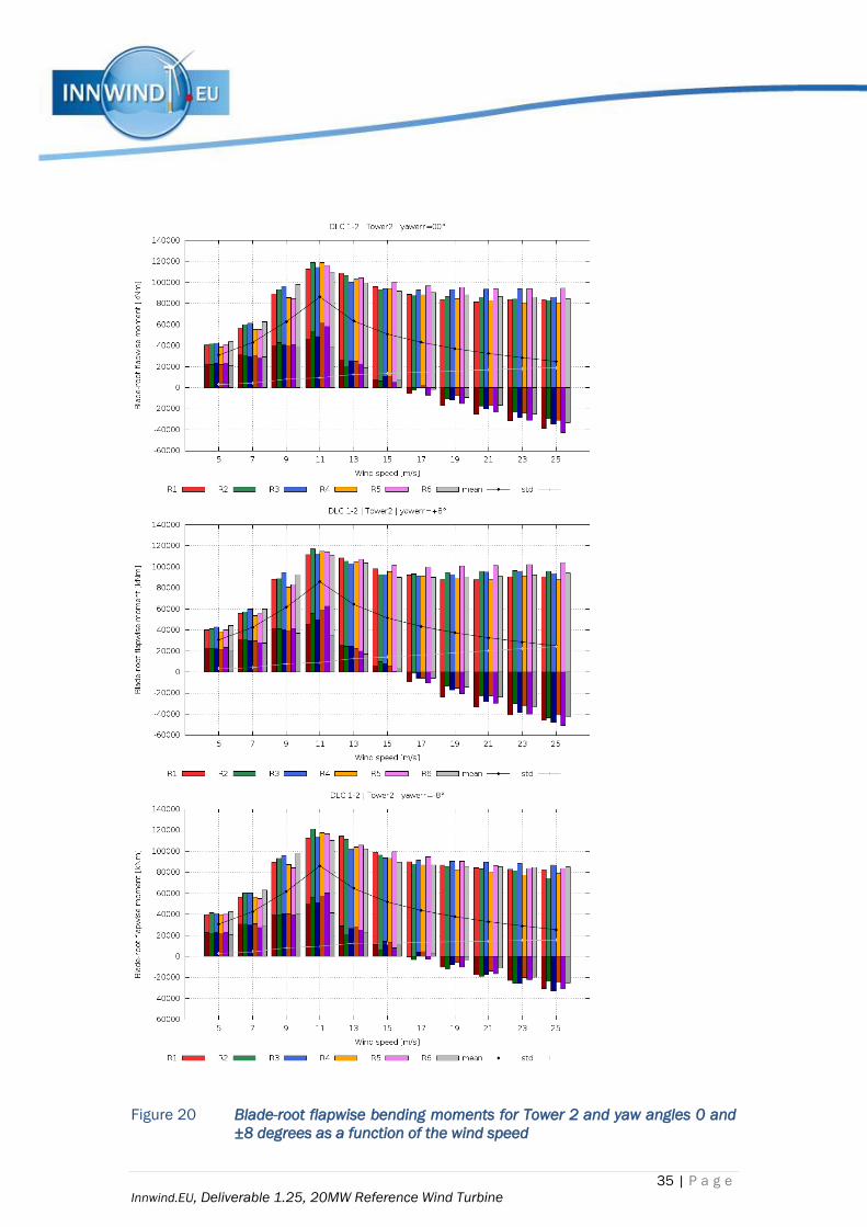
35 | P a g e
Innwind.EU, Deliverable 1.25, 20MW Reference Wind Turbine
Figure 20 Blade-root flapwise bending moments for Tower 2 and yaw angles 0 and
±8 degrees as a function of the wind speed
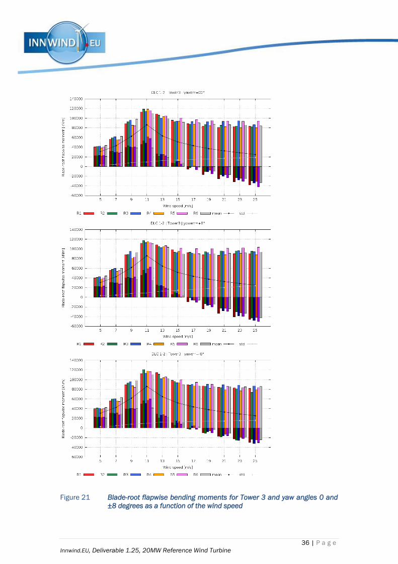
36 | P a g e
Innwind.EU, Deliverable 1.25, 20MW Reference Wind Turbine
Figure 21 Blade-root flapwise bending moments for Tower 3 and yaw angles 0 and
±8 degrees as a function of the wind speed

37 | P a g e
Innwind.EU, Deliverable 1.25, 20MW Reference Wind Turbine
Figure 22 Blade-root edgewise bending moments for Tower 1 and yaw angles 0 and
±8 degrees as a function of the wind speed

38 | P a g e
Innwind.EU, Deliverable 1.25, 20MW Reference Wind Turbine
Figure 23 Blade-root edgewise bending moments for Tower 2 and yaw angles 0 and
±8 degrees as a function of the wind speed

39 | P a g e
Innwind.EU, Deliverable 1.25, 20MW Reference Wind Turbine
Figure 24 Blade-root edgewise bending moments for Tower 3 and yaw angles 0 and
±8 degrees as a function of the wind speed

40 | P a g e
Innwind.EU, Deliverable 1.25, 20MW Reference Wind Turbine
Figure 25 Tower bottom (26m amsl) fore-aft bending moments for Tower 1 and yaw
angles 0 and ±8 degrees as a function of the wind speed
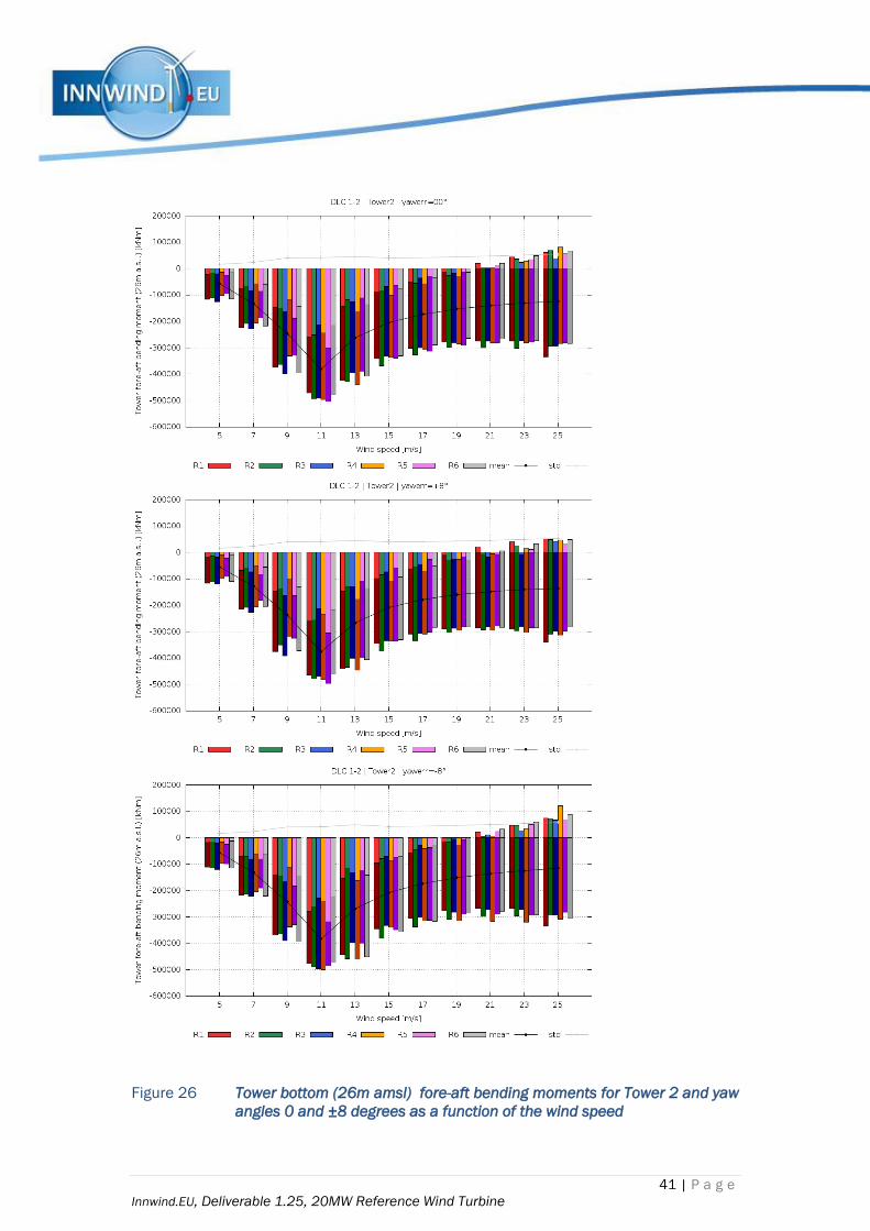
41 | P a g e
Innwind.EU, Deliverable 1.25, 20MW Reference Wind Turbine
Figure 26 Tower bottom (26m amsl) fore-aft bending moments for Tower 2 and yaw
angles 0 and ±8 degrees as a function of the wind speed
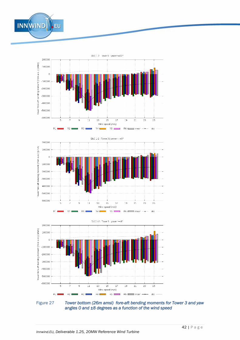
42 | P a g e
Innwind.EU, Deliverable 1.25, 20MW Reference Wind Turbine
Figure 27 Tower bottom (26m amsl) fore-aft bending moments for Tower 3 and yaw
angles 0 and ±8 degrees as a function of the wind speed

43 | P a g e
Innwind.EU, Deliverable 1.25, 20MW Reference Wind Turbine
Figure 28 Tower bottom (26m amsl) side-side bending moments for Tower 1 and
yaw angles 0 and ±8 degrees as a function of the wind speed
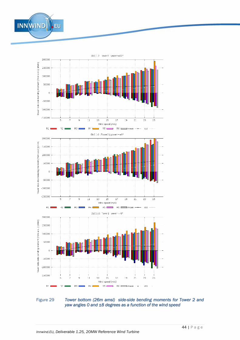
44 | P a g e
Innwind.EU, Deliverable 1.25, 20MW Reference Wind Turbine
Figure 29 Tower bottom (26m amsl) side-side bending moments for Tower 2 and
yaw angles 0 and ±8 degrees as a function of the wind speed

45 | P a g e
Innwind.EU, Deliverable 1.25, 20MW Reference Wind Turbine
Figure 30 Tower bottom (26m amsl) side-side bending moments for Tower 3 and
yaw angles 0 and ±8 degrees as a function of the wind speed
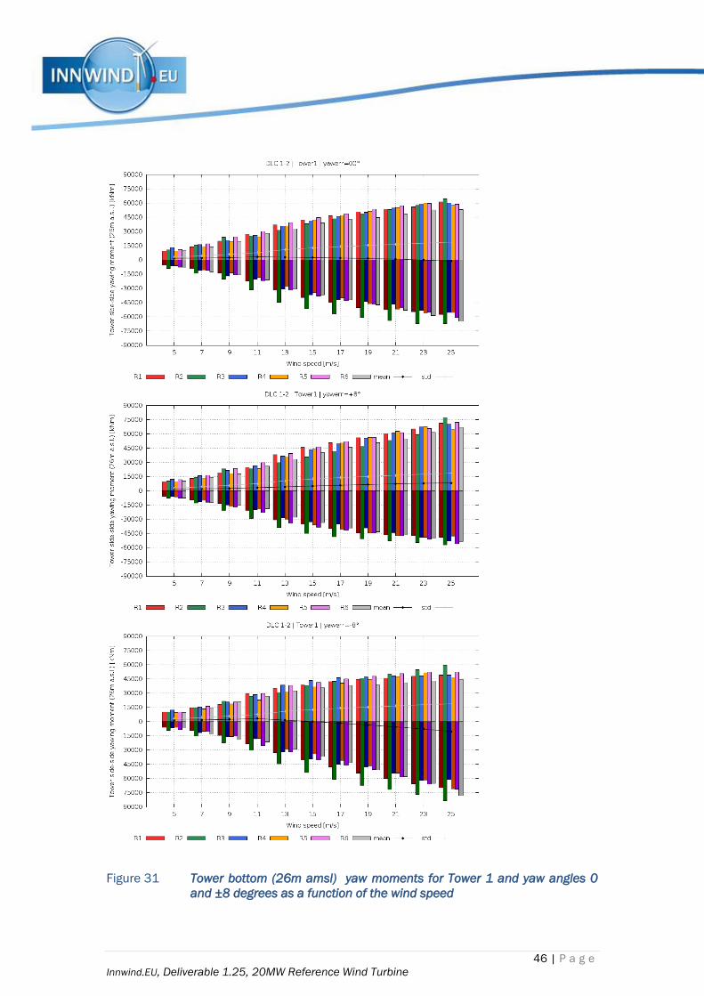
46 | P a g e
Innwind.EU, Deliverable 1.25, 20MW Reference Wind Turbine
Figure 31 Tower bottom (26m amsl) yaw moments for Tower 1 and yaw angles 0
and ±8 degrees as a function of the wind speed

47 | P a g e
Innwind.EU, Deliverable 1.25, 20MW Reference Wind Turbine
Figure 32 Tower bottom (26m amsl) yaw moments for Tower 2 and yaw angles 0
and ±8 degrees as a function of the wind speed

48 | P a g e
Innwind.EU, Deliverable 1.25, 20MW Reference Wind Turbine
Figure 33 Tower bottom (26m amsl) yaw moments for Tower 3 and yaw angles 0
and ±8 degrees as a function of the wind speed
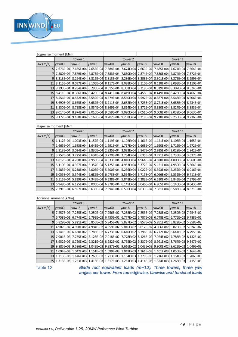
49 | P a g e
Innwind.EU, Deliverable 1.25, 20MW Reference Wind Turbine
Table 12 Blade root equivalent loads (m=12). Three towers, three yaw
angles per tower. From top edgewise, flapwise and torsional loads
Edgewise moment [kNm]
Uw (m/s) yaw00 yaw-8 yaw+8 yaw00 yaw-8 yaw+8 yaw00 yaw-8 yaw+8
5 7.676E+04 7.665E+04 7.653E+04 7.684E+04 7.674E+04 7.663E+04 7.685E+04 7.674E+04 7.664E+04
7 7.880E+04 7.879E+04 7.873E+04 7.883E+04 7.880E+04 7.874E+04 7.880E+04 7.874E+04 7.872E+04
9 8.313E+04 8.294E+04 8.312E+04 8.313E+04 8.286E+04 8.308E+04 8.301E+04 8.275E+04 8.299E+04
11 8.115E+04 8.097E+04 8.106E+04 8.117E+04 8.098E+04 8.110E+04 8.118E+04 8.098E+04 8.110E+04
13 8.293E+04 8.284E+04 8.293E+04 8.315E+04 8.301E+04 8.319E+04 8.319E+04 8.307E+04 8.324E+04
15 8.411E+04 8.386E+04 8.420E+04 8.441E+04 8.419E+04 8.458E+04 8.449E+04 8.428E+04 8.466E+04
17 8.556E+04 8.532E+04 8.559E+04 8.579E+04 8.560E+04 8.597E+04 8.587E+04 8.568E+04 8.606E+04
19 8.690E+04 8.665E+04 8.689E+04 8.711E+04 8.682E+04 8.725E+04 8.721E+04 8.688E+04 8.734E+04
21 8.830E+04 8.788E+04 8.834E+04 8.869E+04 8.814E+04 8.872E+04 8.880E+04 8.827E+04 8.883E+04
23 9.014E+04 8.974E+04 9.010E+04 9.059E+04 9.020E+04 9.051E+04 9.068E+04 9.039E+04 9.063E+04
25 9.172E+04 9.188E+04 9.168E+04 9.202E+04 9.238E+04 9.219E+04 9.218E+04 9.255E+04 9.236E+04
tower 1 tower 2 tower 3
Flapwise moment [kNm]
Uw (m/s) yaw00 yaw-8 yaw+8 yaw00 yaw-8 yaw+8 yaw00 yaw-8 yaw+8
5 1.112E+04 1.093E+04 1.157E+04 1.119E+04 1.102E+04 1.161E+04 1.121E+04 1.103E+04 1.165E+04
7 1.665E+04 1.685E+04 1.643E+04 1.691E+04 1.717E+04 1.668E+04 1.690E+04 1.719E+04 1.672E+04
9 2.913E+04 3.024E+04 2.830E+04 2.935E+04 3.033E+04 2.847E+04 2.935E+04 3.028E+04 2.842E+04
11 3.757E+04 3.725E+04 3.634E+04 3.770E+04 3.734E+04 3.635E+04 3.771E+04 3.735E+04 3.637E+04
13 4.817E+04 4.788E+04 4.950E+04 4.833E+04 4.810E+04 4.964E+04 4.828E+04 4.806E+04 4.960E+04
15 5.110E+04 4.927E+04 5.357E+04 5.125E+04 4.953E+04 5.372E+04 5.121E+04 4.950E+04 5.364E+04
17 5.585E+04 5.238E+04 6.003E+04 5.600E+04 5.256E+04 6.022E+04 5.593E+04 5.252E+04 6.016E+04
19 6.055E+04 5.544E+04 6.685E+04 6.073E+04 5.554E+04 6.715E+04 6.066E+04 5.551E+04 6.711E+04
21 6.515E+04 5.839E+04 7.349E+04 6.538E+04 5.848E+04 7.383E+04 6.530E+04 5.845E+04 7.379E+04
23 6.949E+04 6.125E+04 8.003E+04 6.978E+04 6.145E+04 8.046E+04 6.965E+04 6.140E+04 8.043E+04
25 7.391E+04 6.597E+04 8.633E+04 7.394E+04 6.596E+04 8.633E+04 7.381E+04 6.583E+04 8.621E+04
tower 1 tower 2 tower 3
Torsional moment [kNm]
Uw (m/s) yaw00 yaw-8 yaw+8 yaw00 yaw-8 yaw+8 yaw00 yaw-8 yaw+8
5 7.257E+02 7.255E+02 7.250E+02 7.256E+02 7.258E+02 7.253E+02 7.258E+02 7.259E+02 7.254E+02
7 6.758E+02 6.774E+02 6.799E+02 6.750E+02 6.777E+02 6.787E+02 6.748E+02 6.776E+02 6.788E+02
9 5.829E+02 5.821E+02 5.855E+02 5.845E+02 5.827E+02 5.857E+02 5.851E+02 5.822E+02 5.858E+02
11 4.987E+02 4.990E+02 4.994E+02 4.959E+02 5.016E+02 5.012E+02 4.966E+02 5.025E+02 5.024E+02
13 6.741E+02 6.630E+02 6.783E+02 6.773E+02 6.640E+02 6.798E+02 6.772E+02 6.641E+02 6.795E+02
15 7.901E+02 7.755E+02 8.128E+02 7.918E+02 7.778E+02 8.126E+02 7.924E+02 7.786E+02 8.132E+02
17 8.952E+02 8.720E+02 9.321E+02 8.982E+02 8.755E+02 9.337E+02 8.991E+02 8.767E+02 9.347E+02
19 9.885E+02 9.596E+02 1.042E+03 9.887E+02 9.616E+02 1.043E+03 9.900E+02 9.622E+02 1.046E+03
21 1.094E+03 1.042E+03 1.151E+03 1.099E+03 1.049E+03 1.161E+03 1.101E+03 1.050E+03 1.164E+03
23 1.213E+03 1.146E+03 1.268E+03 1.213E+03 1.154E+03 1.279E+03 1.216E+03 1.154E+03 1.286E+03
25 1.313E+03 1.253E+03 1.413E+03 1.317E+03 1.261E+03 1.414E+03 1.324E+03 1.268E+03 1.415E+03
tower 1 tower 2 tower 3
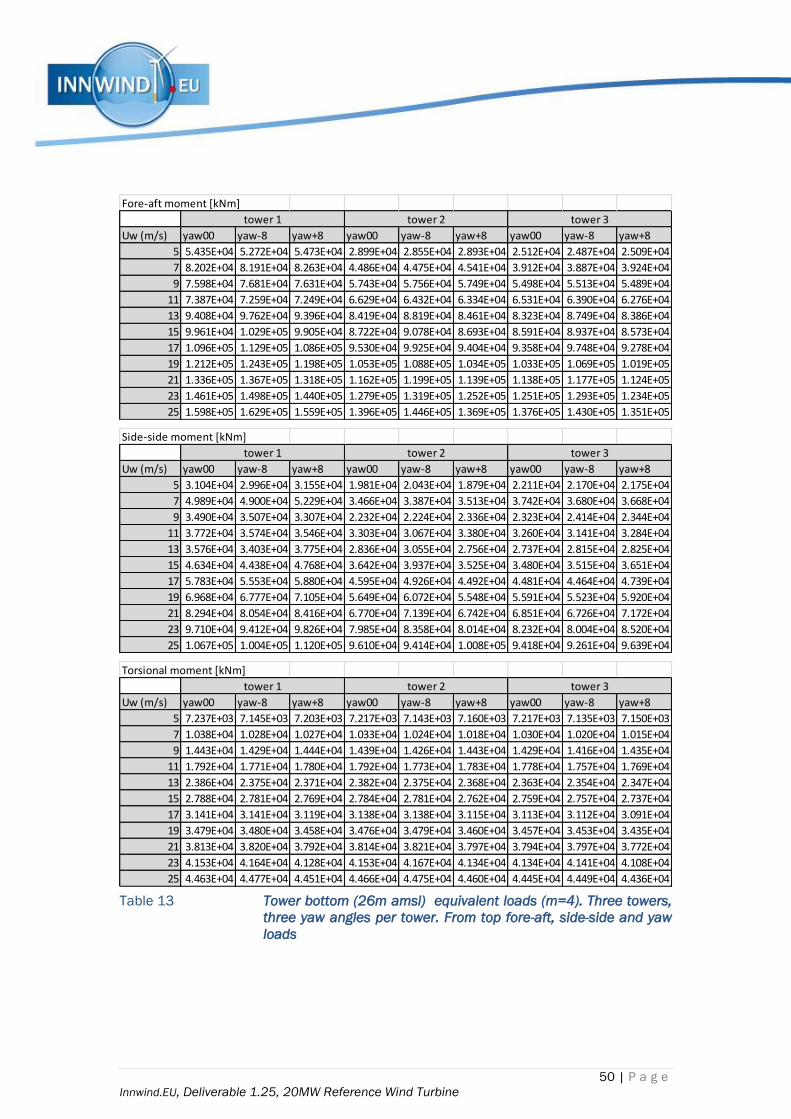
50 | P a g e
Innwind.EU, Deliverable 1.25, 20MW Reference Wind Turbine
Table 13 Tower bottom (26m amsl) equivalent loads (m=4). Three towers,
three yaw angles per tower. From top fore-aft, side-side and yaw
loads
Fore-aft moment [kNm]
Uw (m/s) yaw00 yaw-8 yaw+8 yaw00 yaw-8 yaw+8 yaw00 yaw-8 yaw+8
5 5.435E+04 5.272E+04 5.473E+04 2.899E+04 2.855E+04 2.893E+04 2.512E+04 2.487E+04 2.509E+04
7 8.202E+04 8.191E+04 8.263E+04 4.486E+04 4.475E+04 4.541E+04 3.912E+04 3.887E+04 3.924E+04
9 7.598E+04 7.681E+04 7.631E+04 5.743E+04 5.756E+04 5.749E+04 5.498E+04 5.513E+04 5.489E+04
11 7.387E+04 7.259E+04 7.249E+04 6.629E+04 6.432E+04 6.334E+04 6.531E+04 6.390E+04 6.276E+04
13 9.408E+04 9.762E+04 9.396E+04 8.419E+04 8.819E+04 8.461E+04 8.323E+04 8.749E+04 8.386E+04
15 9.961E+04 1.029E+05 9.905E+04 8.722E+04 9.078E+04 8.693E+04 8.591E+04 8.937E+04 8.573E+04
17 1.096E+05 1.129E+05 1.086E+05 9.530E+04 9.925E+04 9.404E+04 9.358E+04 9.748E+04 9.278E+04
19 1.212E+05 1.243E+05 1.198E+05 1.053E+05 1.088E+05 1.034E+05 1.033E+05 1.069E+05 1.019E+05
21 1.336E+05 1.367E+05 1.318E+05 1.162E+05 1.199E+05 1.139E+05 1.138E+05 1.177E+05 1.124E+05
23 1.461E+05 1.498E+05 1.440E+05 1.279E+05 1.319E+05 1.252E+05 1.251E+05 1.293E+05 1.234E+05
25 1.598E+05 1.629E+05 1.559E+05 1.396E+05 1.446E+05 1.369E+05 1.376E+05 1.430E+05 1.351E+05
tower 1 tower 2 tower 3
Side-side moment [kNm]
Uw (m/s) yaw00 yaw-8 yaw+8 yaw00 yaw-8 yaw+8 yaw00 yaw-8 yaw+8
5 3.104E+04 2.996E+04 3.155E+04 1.981E+04 2.043E+04 1.879E+04 2.211E+04 2.170E+04 2.175E+04
7 4.989E+04 4.900E+04 5.229E+04 3.466E+04 3.387E+04 3.513E+04 3.742E+04 3.680E+04 3.668E+04
9 3.490E+04 3.507E+04 3.307E+04 2.232E+04 2.224E+04 2.336E+04 2.323E+04 2.414E+04 2.344E+04
11 3.772E+04 3.574E+04 3.546E+04 3.303E+04 3.067E+04 3.380E+04 3.260E+04 3.141E+04 3.284E+04
13 3.576E+04 3.403E+04 3.775E+04 2.836E+04 3.055E+04 2.756E+04 2.737E+04 2.815E+04 2.825E+04
15 4.634E+04 4.438E+04 4.768E+04 3.642E+04 3.937E+04 3.525E+04 3.480E+04 3.515E+04 3.651E+04
17 5.783E+04 5.553E+04 5.880E+04 4.595E+04 4.926E+04 4.492E+04 4.481E+04 4.464E+04 4.739E+04
19 6.968E+04 6.777E+04 7.105E+04 5.649E+04 6.072E+04 5.548E+04 5.591E+04 5.523E+04 5.920E+04
21 8.294E+04 8.054E+04 8.416E+04 6.770E+04 7.139E+04 6.742E+04 6.851E+04 6.726E+04 7.172E+04
23 9.710E+04 9.412E+04 9.826E+04 7.985E+04 8.358E+04 8.014E+04 8.232E+04 8.004E+04 8.520E+04
25 1.067E+05 1.004E+05 1.120E+05 9.610E+04 9.414E+04 1.008E+05 9.418E+04 9.261E+04 9.639E+04
tower 1 tower 2 tower 3
Torsional moment [kNm]
Uw (m/s) yaw00 yaw-8 yaw+8 yaw00 yaw-8 yaw+8 yaw00 yaw-8 yaw+8
5 7.237E+03 7.145E+03 7.203E+03 7.217E+03 7.143E+03 7.160E+03 7.217E+03 7.135E+03 7.150E+03
7 1.038E+04 1.028E+04 1.027E+04 1.033E+04 1.024E+04 1.018E+04 1.030E+04 1.020E+04 1.015E+04
9 1.443E+04 1.429E+04 1.444E+04 1.439E+04 1.426E+04 1.443E+04 1.429E+04 1.416E+04 1.435E+04
11 1.792E+04 1.771E+04 1.780E+04 1.792E+04 1.773E+04 1.783E+04 1.778E+04 1.757E+04 1.769E+04
13 2.386E+04 2.375E+04 2.371E+04 2.382E+04 2.375E+04 2.368E+04 2.363E+04 2.354E+04 2.347E+04
15 2.788E+04 2.781E+04 2.769E+04 2.784E+04 2.781E+04 2.762E+04 2.759E+04 2.757E+04 2.737E+04
17 3.141E+04 3.141E+04 3.119E+04 3.138E+04 3.138E+04 3.115E+04 3.113E+04 3.112E+04 3.091E+04
19 3.479E+04 3.480E+04 3.458E+04 3.476E+04 3.479E+04 3.460E+04 3.457E+04 3.453E+04 3.435E+04
21 3.813E+04 3.820E+04 3.792E+04 3.814E+04 3.821E+04 3.797E+04 3.794E+04 3.797E+04 3.772E+04
23 4.153E+04 4.164E+04 4.128E+04 4.153E+04 4.167E+04 4.134E+04 4.134E+04 4.141E+04 4.108E+04
25 4.463E+04 4.477E+04 4.451E+04 4.466E+04 4.475E+04 4.460E+04 4.445E+04 4.449E+04 4.436E+04
tower 1 tower 2 tower 3

PROPRIETARY RIGHTS STATEMENT
This document contains information, which is proprietary to the “INNWIND.EU” Consortium. Neither this document nor
the information contained herein shall be used, duplicated or communicated by any means to any third party, in whole
or in parts, except with prior written consent of the “INNWIND.EU” consortium.
Deliverable 1.25b
Reliability Level Estimation of a 20MW Jacket Structure
October 2017
Agreement n.: 308974
Duration November 2012 – October 2017
DTU Wind
The research leading to these results has received funding from
the European Community’s Seventh Framework Programme
under grant agreement
2 | P a g e
(Innwind.EU, Deliverable 1.25b, Reliability Level Estimation of a 20MW Jacket Structure)
Document information
Document Name: Reliability Level Estimation of a 20MW Jacket Structure
Document Number: Deliverable 1.25b
Author: Tomas Gintautas, John Dalsgaard Soerensen (AAU)
Document Type Report
Dissemination level PU
Review: John Dalsgaard Soerensen
Date: October 2017
WP: WP1: Conceptual Design
Task: Task 1.2: Assessment of Innovation at the Subsystems Level
Approval: Approved by WP Leader
3 | P a g e
(Innwind.EU, Deliverable 1.25b, Reliability Level Estimation of a 20MW Jacket Structure)
TABLE OF CONTENTS
LIST OF FIGURES ...................................................................................................................................... 4
1. INTRODUCTION / SUMMARY ............................................................................................................ 5
2. RELIABILITY-BASED INSPECTION PLANNING ................................................................................... 5 1.1 Probabilistic modelling of inspections ................................................................................... 7
3. PROBABILISTIC MODELLING OF FATIGUE ........................................................................................ 8 3.1 Stochastic model based on SN curves .................................................................................. 8 3.2 Fracture mechanis based stochastic model for fatigue crack growth .............................. 10
4. SYSTEM EFFECTS ........................................................................................................................... 13
5. RESULTS FOR 20MW JACKET STRUCTURE .................................................................................. 14 5.1 Reliability level estimation for individual elements and Fracture mechanics model
calibration .......................................................................................................................................... 14 5.2 System reliability and uncertainty correlation .................................................................... 18 5.3 Effects of inspections .......................................................................................................... 19
6. REFERENCES .................................................................................................................................. 22
4 | P a g e
(Innwind.EU, Deliverable 1.25b, Reliability Level Estimation of a 20MW Jacket Structure)
LIST OF FIGURES
Figure 1.1. Illustration of inspection plan with equidistant inspections. ...............................................6 Figure 1.2. Illustration of inspection plan where inspections are performed when the annual
probability of failure exceeds the maximum acceptable annual probability of failure. .........................7 Figure 2.1: Weld geometry parameters for crack growth model, [64]. ............................................... 10 Equations (14) and (15) are a discretized version of (11) and (12), representing crack growth in two
directions (depth ‘a’ and width ‘c’), hence the summations. Also, use of sets of two A and K
parameters comes from the use of bi-linear crack growth model (A1,K1 for Stage A and A2, K2 for
Stage B in Figure 2.2). ............................................................................................................................ 10 Figure 2.3.: Procedure for crack growth calculation (a) [3] and Paris law sketch (b) [6] ................... 12 Figure 4.1.: Elements/nodes selected for the analysis [9], ................................................................. 14 Figure 4.2.: Stress range spectra for the selected elements (most critical node), based on [9], ..... 15 Figure 4.3.: Results of SN analysis of the selected elements. ............................................................ 16 Figure 4.4.: Results of FM model calibration for the selected elements. ........................................... 18 Figure 4.5.: Results of system reliability analysis with and without correlation. ................................ 19 Figure 4.6.: Annual system reliability indexes using Close Visual Inspections assuming moderately
easy access. ............................................................................................................................................ 20 Figure 4.7.: Annual system reliability indexes using Close Visual Inspections assuming easy access.
................................................................................................................................................................. 20 Figure 4.8.: Annual system reliability indexes using Eddy Current Inspections. ................................. 21 Figure 4.9.: Annual system reliability indexes using Ultrasonic Inspections. ...................................... 21 Figure 4.10.: Optimal inspection intervals for 20MW jacket substructure (system) using different
inspection techniques. ........................................................................................................................... 22
5 | P a g e
(Innwind.EU, Deliverable 1.25b, Reliability Level Estimation of a 20MW Jacket Structure)
1. INTRODUCTION / SUMMARY
The objective of this report is to present and apply a reliability-based approach for
assessment of the system reliability of fatigue critical details in very large support
structures and to evaluate the potentials for verification of satisfactory reliability for
fatigue critical details using inspections. Further to include the effect of correlation
between failure modes in different fatigue failure modes, and to investigate the effect in
generic case studies relevant for very large support structures.
Verification of sufficient reliability using safety factors as traditionally done in design
standards such as the IEC 61400 series (and the Eurocodes) does not allow in a
consistent way to account for the effect of inspections done during the design lifetime.
This report describes the theoretical basis for reliability-based planning of inspections
(Bayesian pre-posterior decision theory). This requires that a probabilistic fracture
mechanics model is calibrated to result in the same reliability level as obtained using the
SN-curve approach used in traditional design standards. This includes establishment of
stochastic models for load and fatigue strength parameters. These steps are described in
this report. It is noted that a system reliability-based assessment / planning of inspections
are very computer-time demanding, and needs careful modelling of the uncertainties. In
this report experience from JCSS (Joint Committee on Structural Safety) and from
applications in other offshore industries is applied.
The results indicate large potentials in using inspections for increasing the design lifetime
fulfilling requirements to a minimum reliability level. E.g. an example shows that 3-4
inspections during the design lifetime of 25 years may increase the safe lifetime from 13
years to 25 years. It is noted that for decision making on the use of inspections a cost
consideration should be performed where the following costs are compared:
costs of inspections and eventual maintenance/repair in case of detected cracks
cost savings in a reduced cost of the support structure, incl. the cost of additional
steel to be used in the support structure such that it fulfils the reliability
requirements in the design standards
The case studies performed indicate that the correlation (mainly from common epistemic
uncertainties) between different fatigue failure modes is limited and does not have a
significant influence on the system reliability.
2. RELIABILITY-BASED INSPECTION PLANNING
Inspection planning procedures require in principle information on costs of
design/manufacturing, failures, inspections and repairs. Often these are not available, and
the inspection planning is based on the requirement that the annual probability of failure
in all years has to satisfy a reliability constraint. This implies that the annual probabilities
of fatigue failure for all years during the operational life of the structure has to fulfill:
(1)
The implicit code requirements to the safety of the structures in regard to total collapse
may be assessed through the annual probability of fatigue failure of critical details (in the
last year in service) PFAT,j for a joint for which the consequences of failure are “substantial”
jj ACFAT PP

6 | P a g e
(Innwind.EU, Deliverable 1.25b, Reliability Level Estimation of a 20MW Jacket Structure)
(i.e. the Design Fatigue Factor (DFF) is equal to 10 for offshore structures in general (oil
and gas) and equal to 3 for offshore wind turbines). This probability can be regarded an
acceptance criteria i.e. PAC. A typical maximum acceptable annual probability of collapse
failure is in the in the range 10-4 - 3·10-5 for unmanned structures, see e.g. [1] and [2]. On
this basis it is possible to establish joint & member specific acceptance criteria in regard
to fatigue failure. For each critical detail / joint j the conditional probability of structural
collapse given fatigue failure of the considered joint PCOL|FAT,j are determined and the
individual joint acceptance criteria for the annual probability of joint fatigue failure are
found as:
(2)
The annual probability of fatigue failure PFAT,j may be determined on the basis of either a
simplified probabilistic SN approach or a probabilistic fracture mechanics approach. As an
alternative to the above approach where basis is taken in annual probabilities of failure it
is equally possible to take basis in service life probabilities. However, as most installation
concept risk analyses give requirements to the maximum allowable risk for structural
collapse in terms of annual failure probabilities, these are used in the following.
Further, in risk- and reliability-based inspection planning the planning is often made with
the assumption that no cracks are found at the inspections. If a crack is found, then a
repair is typically performed and a new inspection plan has to be made based on the
observation. If all inspections are made with the same time intervals, then the annual
probability of fatigue failure as a function of time could be as illustrated in Figure 2.1.
Figure 2.1. Illustration of inspection plan with equidistant inspections.
If inspections are made when the annual probability of fatigue failure exceeds the critical
value then inspections are made with different time intervals, as illustrated in Figure 2.2.
As assumed above, it is often assumed that the inspection planning can be based on the
no-find assumption. This way of inspection planning is the one which if most often used.
Often this approach results in increasing time intervals between inspections.
j
j
FATCOL
AC
ACP
PP
jACP
)(tPjFAT
1T 2T 3T t4T
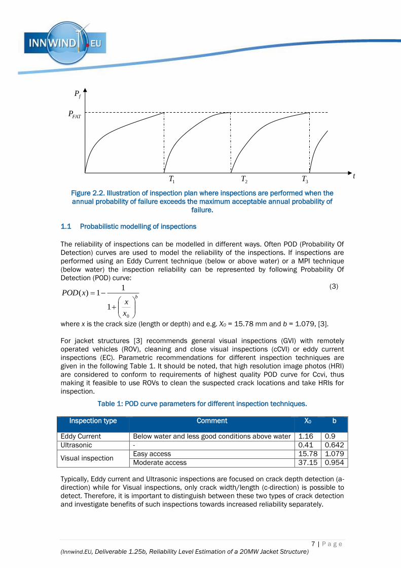
7 | P a g e
(Innwind.EU, Deliverable 1.25b, Reliability Level Estimation of a 20MW Jacket Structure)
Figure 2.2. Illustration of inspection plan where inspections are performed when the
annual probability of failure exceeds the maximum acceptable annual probability of
failure.
1.1 Probabilistic modelling of inspections
The reliability of inspections can be modelled in different ways. Often POD (Probability Of
Detection) curves are used to model the reliability of the inspections. If inspections are
performed using an Eddy Current technique (below or above water) or a MPI technique
(below water) the inspection reliability can be represented by following Probability Of
Detection (POD) curve:
(3)
where x is the crack size (length or depth) and e.g. X0 = 15.78 mm and b = 1.079, [3].
For jacket structures [3] recommends general visual inspections (GVI) with remotely
operated vehicles (ROV), cleaning and close visual inspections (cCVI) or eddy current
inspections (EC). Parametric recommendations for different inspection techniques are
given in the following Table 1. It should be noted, that high resolution image photos (HRI)
are considered to conform to requirements of highest quality POD curve for Ccvi, thus
making it feasible to use ROVs to clean the suspected crack locations and take HRIs for
inspection.
Table 1: POD curve parameters for different inspection techniques.
Inspection type Comment X0 b
Eddy Current Below water and less good conditions above water 1.16 0.9
Ultrasonic - 0.41 0.642
Visual inspection Easy access 15.78 1.079
Moderate access 37.15 0.954
Typically, Eddy current and Ultrasonic inspections are focused on crack depth detection (a-
direction) while for Visual inspections, only crack width/length (c-direction) is possible to
detect. Therefore, it is important to distinguish between these two types of crack detection
and investigate benefits of such inspections towards increased reliability separately.
b
x
xxPOD
0
1
11)(
FATP
fP
1T 2T 3T t

8 | P a g e
(Innwind.EU, Deliverable 1.25b, Reliability Level Estimation of a 20MW Jacket Structure)
If an inspection has been performed at time TI and no cracks are detected then the
probability of failure can be updated by
, (4)
where h(t) is a limit state modeling the crack detection. If the inspection technique is
related to the crack length then h(t) is written:
(5)
Here c(t) is the crack length at time t and cd is smallest detectable crack length. cd is
modelled by a stochastic variable with distribution function equal to the POD-curve:
(6)
Similarly if the inspection technique is related to the crack depth then h(t) is written:
(7)
where a(t) is the crack length at time t and ad is smallest detectable crack length. ad
is
modelled by a stochastic variable with distribution function equal to the POD-curve:
(8)
If two independent inspections are performed at time TI and no cracks are detected then
the probability of failure can be updated by
, (9)
where and are the limit states modeling the
inspections.
3. PROBABILISTIC MODELLING OF FATIGUE
Probabilistic models for fatigue failure are in general established using the SN-approach
together with the Miners rule of linear fatigue damage accumulation. SN-test results are
used to model the uncertainty related to the SN-curves. However, the probabilistic model
based on SN-curves cannot be used investigate the effect of inspections on the reliability
levels since SN-curves do not have information about the crack size. Therefore, a
probabilistic fracture mechanics approach is needed where an explicit measure of the
fatigue crack is represented. Traditionally in reliability- and risk-based inspection planning
(RBI) the probabilistic fracture mechanics model is calibrated to give the same reliability
as function of time as obtained by the SN-approach. This approach is also applied in the
following sections.
3.1 Stochastic model based on SN curves
Fatigue reliability is assessed using the SN-curve approach together with Miner’s rule,
combined in the following limit state equation:
00 at timedetection -no II
U
F ThtgPTtP ITt
tccth d
xPODxFdc )(
taath d
xPODxFda )(
000 at timedetection -no 21 III
U
F ThThtgPTtP ITt
Id Taath 11 Id Taath
22
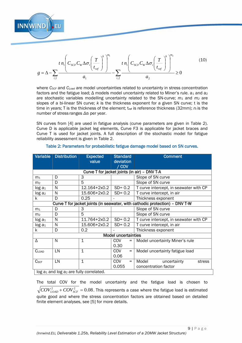
9 | P a g e
(Innwind.EU, Deliverable 1.25b, Reliability Level Estimation of a 20MW Jacket Structure)
0
2, 21, 1
21
i
mk
ref
iWSCFi
i
mk
ref
iWSCFi
a
t
TCCnt
a
t
TCCnt
g
(10)
where CSCF and CLoad are model uncertainties related to uncertainty in stress concentration
factors and the fatigue load; Δ models model uncertainty related to Miner’s rule. a1 and a2
are stochastic variables modelling uncertainty related to the SN-curve; m1 and m2 are
slopes of a bi-linear SN curve; k is the thickness exponent for a given SN curve; t is the
time in years; T is the thickness of the element; tref is reference thickness (32mm); ni is the
number of stress ranges Δσi per year.
SN curves from [4] are used in fatigue analysis (curve parameters are given in Table 2).
Curve D is applicable jacket leg elements, Curve F3 is applicable for jacket braces and
Curve T is used for jacket joints. A full description of the stochastic model for fatigue
reliability assessment is given in Table 2.
Table 2: Parameters for probabilistic fatigue damage model based on SN curves.
Variable Distribution Expected
value
Standard
deviation
/ COV
Comment
Curve T for jacket joints (in air) – DNV T-A
m1 D 3 Slope of SN curve
m2 D 5 Slope of SN curve
log a1 N 12.164+2x0.2 SD= 0.2 T curve intercept, in seawater with CP
log a2 N 15.606+2x0.2 SD= 0.2 T curve intercept, in air
k D 0.25 - Thickness exponent
Curve T for jacket joints (in seawater, with cathodic protection) – DNV T-W
m1 D 3 Slope of SN curve
m2 D 5 Slope of SN curve
log a1 N 11.764+2x0.2 SD= 0.2 T curve intercept, in seawater with CP
log a1 N 15.606+2x0.2 SD= 0.2 T curve intercept, in air
k D 0.2 - Thickness exponent
Model uncertainties
Δ N 1 COV =
0.30
Model uncertainty Miner’s rule
CLOAD LN 1 COV =
0.06
Model uncertainty fatigue load
CSCF LN 1 COV =
0.055
Model uncertainty stress
concentration factor
log a1 and log a2 are fully correlated.
The total COV for the model uncertainty and the fatigue load is chosen to
08.022 SCFLOAD COVCOV . This represents a case where the fatigue load is estimated
quite good and where the stress concentration factors are obtained based on detailed
finite element analyses, see [5] for more details.

10 | P a g e
(Innwind.EU, Deliverable 1.25b, Reliability Level Estimation of a 20MW Jacket Structure)
3.2 Fracture mechanis based stochastic model for fatigue crack growth
The applied fatigue crack growth model (based on fracture mechanics) is bi-linear and
crack growth is considered in both ‘c’ and ‘a’ (depth and width) directions, see Figure 3.1,
right side. The model is generally based on [6] with crack growth parameters adopted from
[7] where necessary. The crack growth is typically described by the following coupled
differential equations:
00 )()( aNaKAdN
da m
aa (11)
00 )()( cNcKAdN
dc m
cc (12)
here Aa, Ac and m are material parameters, a0 and c0 describe the crack depth a and crack
length c, respectively, after N1 cycles and where the stress intensity ranges are ΔKa(Δσ)
and ΔKa(Δσ).
Failure is considered when a crack grows through the thickness of the monopile/transition
piece steel and can be summarized in the following limit state function:
0)(),( taatXg cr (13)
Figure 3.1: Weld geometry parameters for crack growth model, [64].
where t is time (in years) in the time interval between 0 and service life TL. Crack
dimensions at any given time within turbines service life can be calculated using following
equations:
21
1,
2,,22,
1,
1,,11,)(m
j
jaSIFj
m
i
iaSIFi KCANKCANta (14)
21
1,
2,,22,
1,
1,,11,)(m
j
jcSIFj
m
i
icSIFi KCANKCANtc (15)
Equations (14) and (15) are a discretized version of (11) and (12), representing crack
growth in two directions (depth ‘a’ and width ‘c’), hence the summations. Also, use of sets
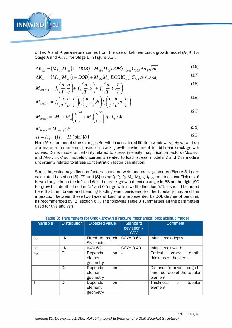
11 | P a g e
(Innwind.EU, Deliverable 1.25b, Reliability Level Estimation of a 20MW Jacket Structure)
of two A and K parameters comes from the use of bi-linear crack growth model (A1,K1 for
Stage A and A2, K2 for Stage B in Figure 3.2).
iiSCFLoadbakbamakmaai aCCDOBMMDOBMMK 1, (16)
iiSCFLoadbckbcmckmcci aCCDOBMMDOBMMK 1, (17)
T
L
T
af
T
af
c
a
T
afM abkm ,,,, 221)(
(18)
T
L
c
a
T
af
c
a
T
af
T
L
a
c
T
afM cbkm ,,,,,,, 221)(
(19)
/
4
3
2
21)( fgc
aM
c
aMMM cma
(20)
HMM cmacba )()( (21)
qHHHH sin)( 121 (22)
Here Ni is number of stress ranges Δσi within considered lifetime window; A1, A2 m1 and m2
are material parameters based on crack growth environment for bi-linear crack growth
curves; CSIF is model uncertainty related to stress intensity magnification factors (Mkm(b)a(c)
and Mm(b)a(c)); CLOAD models uncertainty related to load (stress) modelling and CSCF models
uncertainty related to stress concentration factor calculation.
Stress intensity magnification factors based on weld and crack geometry (Figure 3.1) are
calculated based on [3], [7] and [8] using f1, f2, f3, M1, M2, g, fΘ geometrical coefficients. θ
is weld angle in on the left and Θ is the crack growth direction angle in 68 on the right (90
for growth in depth direction “a” and 0 for growth in width direction “c”). It should be noted
here that membrane and bending loading was considered for the tubular joints, and the
interaction between these two types of loading is represented by DOB-degree of bending,
as recommended by [3] section 6.7. The following Table 3 summarizes all the parameters
used for this analysis.
Table 3: Parameters for Crack growth (Fracture mechanics) probabilistic model
Variable Distribution Expected value Standard
deviation /
COV
Comment
a0 LN Fitted to match
SN results
COV= 0.66 Initial crack depth
c0 LN a0/0.62 COV= 0.40 Initial crack width
acr D Depends on
element
geometry
- Critical crack depth,
thickens of the steel.
L D Depends on
element
geometry
- Distance from weld edge to
inner surface of the tubular
element
T D Depends on
element
geometry
- Thickness of tubular
element
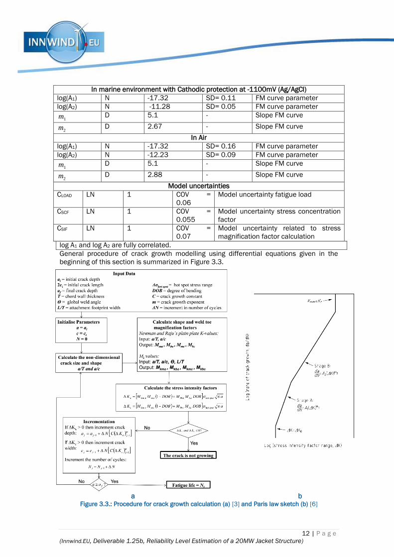
12 | P a g e
(Innwind.EU, Deliverable 1.25b, Reliability Level Estimation of a 20MW Jacket Structure)
In marine environment with Cathodic protection at -1100mV (Ag/AgCl)
log(A1) N -17.32 SD= 0.11 FM curve parameter
log(A2) N -11.28 SD= 0.05 FM curve parameter
D 5.1 - Slope FM curve
D 2.67 - Slope FM curve
In Air
log(A1) N -17.32 SD= 0.16 FM curve parameter
log(A2) N -12.23 SD= 0.09 FM curve parameter
D 5.1 - Slope FM curve
D 2.88 - Slope FM curve
Model uncertainties
CLOAD LN 1 COV =
0.06
Model uncertainty fatigue load
CSCF LN 1 COV =
0.055
Model uncertainty stress concentration
factor
CSIF LN 1 COV =
0.07
Model uncertainty related to stress
magnification factor calculation
log A1 and log A2 are fully correlated.
General procedure of crack growth modelling using differential equations given in the
beginning of this section is summarized in Figure 3.3.
a b Figure 3.3.: Procedure for crack growth calculation (a) [3] and Paris law sketch (b) [6]
1m
2m
1m
2m

13 | P a g e
(Innwind.EU, Deliverable 1.25b, Reliability Level Estimation of a 20MW Jacket Structure)
The transition (“knee”) point between stages A and B in Figure 3.3 is calculated based on
realizations of log(A1), log(A1), m1 and m2 using the following equation:
12
21 )log()log()log(
mm
AAKtrans
(23)
As recommended in [3] the following additional geometrical parameters for tubular jacket
joints/elements are assumed (based on HSE joint database data):
TPWeld TL 17.1
043Weld
81.0DOB
4. SYSTEM EFFECTS
Since the jacket substructure contains multiple structural members and system failure /
total collapse / major damage may occur if one of the structural members fail, the system
reliability is estimated considering a series system model consisting of potential failure in
any of the structural members as elements in the series system model. It is noted that
some additional load bearing capacity may exist in case of failure of a structural member.
Assessment of this additional resistance requires non-linear finite element analysis which
is outside the scope of this investigation. The system probability of failure for a series
system with m elements / fatigue failure critical details is estimated by:
)(10)(1
ρβ;X m
m
ii
S
f gPP
(24)
where Φm(.) is the standardized m-dimensional Normal distribution function, β is the
vector with reliability indices and the elements in the correlation matrix, ρ are obtained
from ρij= αiT αj. The α-vector aj is obtained as
TLRj j straeroexpdy n XXXX ,,,,,,0,...,0,0,,...,0,0 α (25)
where the index indicates which stochastic variable the α -value is connected to. It is noted
that the ‘fatigue strength’ R for different structural members are assumed statistically
independent.
The system reliability index is defined as
S
fS P1 (26)

14 | P a g e
(Innwind.EU, Deliverable 1.25b, Reliability Level Estimation of a 20MW Jacket Structure)
5. RESULTS FOR 20MW JACKET STRUCTURE
This section shows the results of methodology presented in sections 1 through 4. The
focus is on the 20 MW wind turbine reference jacket substructure, designed by Ramboll
and documented in [9] and [10]. The following Figure 5.1 shows the locations of selected
elements together with their notation as given in [9].
Figure 5.1.: Elements/nodes selected for the analysis [9],
4 different types of joints are selected for the reliability analysis and inspection planning.
The considered elements/joints are as follows:
1. Node 13A0P0 – K joint with expected characteristic lifetime of 60 years (below
mean water level). Tubular element thickness 34.9 mm.
2. Node 15AA00 – X joint with expected characteristic lifetime of 41 years (below
mean water level). Tubular element thickness 31.8 mm.
3. Node 20A0P0 – K joint with expected characteristic lifetime of 45 years (below
mean water level). Tubular element thickness 34.9mm.
4. Node 50A0P0 – K joint with expected characteristic lifetime of 85 years (above
mean water level). Tubular element thickness 25.4mm.
5.1 Reliability level estimation for individual elements and Fracture mechanics model
calibration
Stress range spectra were provided by WP4 partners for the joints mentioned above in
terms of expected stress ranges and their respective half-cycle counts. The following
Figure 5.2 shows the stress range spectra for the 4 selected joints. The 20MW wind

15 | P a g e
(Innwind.EU, Deliverable 1.25b, Reliability Level Estimation of a 20MW Jacket Structure)
turbine jacket substructure design is not finalized yet and the stress range spectra used in
this analysis is based on the “Preliminary design results” from [9]. Furthermore, it should
be noted that the stress range spectra were provided at 12 nodes around the tubular
member cross-section circumferentially. Only one most critical node per element was
selected based on maximum equivalent damage stress range Δσeq:
m
n
i
i
n
i
m
ii
eq
N
N
/1
1
1
(27)
Figure 5.2.: Stress range spectra for the selected elements (most critical node), based on [9],
Using the stress range spectra, the reliability levels for all 4 elements are estimated using
SN curve approach combined with miners rule, as described in section 3.1. It should be
noted here that [9] provides only characteristic estimates of expected fatigue lives of the
jacket elements – the fatigue load spectra used for fatigue life estimation have a safety
factor γF=1.0 and modelling and load uncertainties are accounted for by using a Design
Fatigue Factor (DFF=3). This implies increasing the required design life from 25 to 75
years. However, for probabilistic inspection planning, it is important to take the relevant
uncertainties into account directly into the failure function (eq. (10)) through stochastic
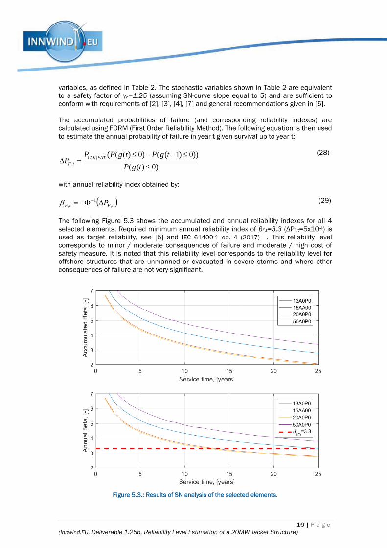
16 | P a g e
(Innwind.EU, Deliverable 1.25b, Reliability Level Estimation of a 20MW Jacket Structure)
variables, as defined in Table 2. The stochastic variables shown in Table 2 are equivalent
to a safety factor of γF=1.25 (assuming SN-curve slope equal to 5) and are sufficient to
conform with requirements of [2], [3], [4], [7] and general recommendations given in [5].
The accumulated probabilities of failure (and corresponding reliability indexes) are
calculated using FORM (First Order Reliability Method). The following equation is then used
to estimate the annual probability of failure in year t given survival up to year t:
)0)((
))0)1(()0)(((|
,
tgP
tgPtgPPP
FATCOL
tF
(28)
with annual reliability index obtained by:
tFtF P ,
1
, (29)
The following Figure 5.3 shows the accumulated and annual reliability indexes for all 4
selected elements. Required minimum annual reliability index of βF,t=3.3 (ΔPF,t=5x10⁻⁴) is
used as target reliability, see [5] and IEC 61400-1 ed. 4 (2017) . This reliability level
corresponds to minor / moderate consequences of failure and moderate / high cost of
safety measure. It is noted that this reliability level corresponds to the reliability level for
offshore structures that are unmanned or evacuated in severe storms and where other
consequences of failure are not very significant.
Figure 5.3.: Results of SN analysis of the selected elements.

17 | P a g e
(Innwind.EU, Deliverable 1.25b, Reliability Level Estimation of a 20MW Jacket Structure)
It is seen that elements / fatigue critical details have different reliability levels and thus
different expected ‘safe’ lifetimes, thus implying that system effects should be cosidered
and annual system reliability should be estimated. This is done and documented in section
5.2. It is also seen that some elements have insufficient reliability. One possibility to
increase the reliability is to perform inspections, see below following te approach
described above.
Using the model described in set ion 3.2, Fracture Mechanics model is calibrated to give
approximately the same annual reliability indices as function of time as obtained above
with SN-curves from the [11]. The calibration parameter in the model is initial crack depth
a0. The calibration is performed in such a way that the predicted annual reliability indexes
match at 10-25 years of service, because typically Fracture mechanics models are less
reliable for the first few years of service. The following Figure 5.4 shows the results of FM
model calibration for all 4 selected elements and it can be concluded that a very good
match is obtained - the curves are very similar and “failure time” (βF,t ≤ 3.3) is predicted
very accurately by the Fracture Mechanics model for all the elements.
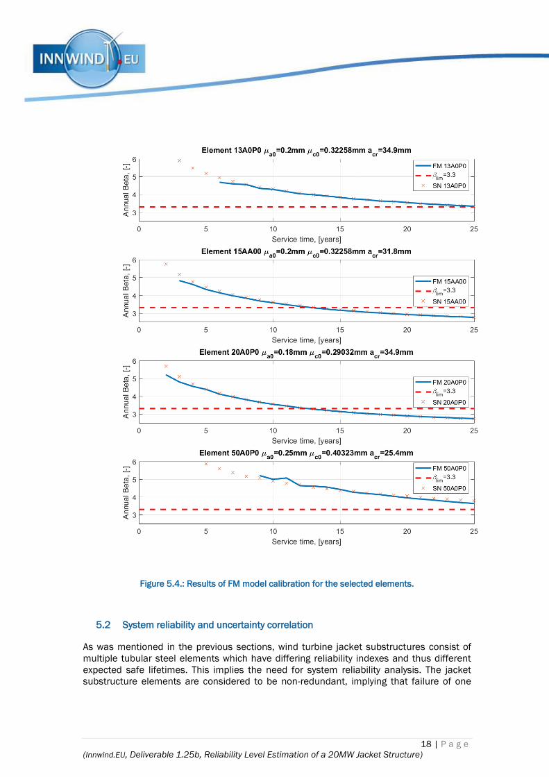
18 | P a g e
(Innwind.EU, Deliverable 1.25b, Reliability Level Estimation of a 20MW Jacket Structure)
Figure 5.4.: Results of FM model calibration for the selected elements.
5.2 System reliability and uncertainty correlation
As was mentioned in the previous sections, wind turbine jacket substructures consist of
multiple tubular steel elements which have differing reliability indexes and thus different
expected safe lifetimes. This implies the need for system reliability analysis. The jacket
substructure elements are considered to be non-redundant, implying that failure of one
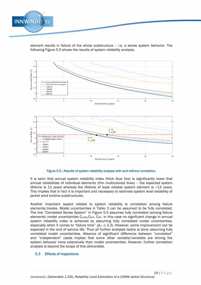
19 | P a g e
(Innwind.EU, Deliverable 1.25b, Reliability Level Estimation of a 20MW Jacket Structure)
element results in failure of the whole substructure – i.e. a series system behavior. The
following Figure 5.5 shows the results of system reliability analysis.
Figure 5.5.: Results of system reliability analysis with and without correlation.
It is seen that annual system reliability index (thick blue line) is significantly lower that
annual reliabilities of individual elements (thin multicolored lines) – the expected system
lifetime is 11 years whereas the lifetime of least reliable system element is ~13 years.
This implies that in fact it is important and necessary to estimate system level reliability of
jacket wind turbine substructures.
Another important aspect related to system reliability is correlation among failure
elements/modes. Model uncertainties in Table 3 can be assumed to be fully correlated.
The line “Correlated Series System” in Figure 5.5 assumes fully correlated (among failure
elements) model uncertainties CLOAD,CSCF, CSIF. In this case no significant change in annual
system reliability index is achieved by assuming fully correlated model uncertainties,
especially when it comes to “failure time” (βF,t ≤ 3.3). However, some improvement can be
expected in the end of service life. Thus all further analyses below is done assuming fully
correlated model uncertainties. Absence of significant difference between “correlated”
and “independent” cases implies that some other variable/variables are driving the
system behavior more extensively than model uncertainties. However, further correlation
analysis is beyond the scope of this deliverable.
5.3 Effects of inspections

20 | P a g e
(Innwind.EU, Deliverable 1.25b, Reliability Level Estimation of a 20MW Jacket Structure)
The calibrated FM model is used to introduce inspections in order to maintain annual
reliability levels above the βF,t = 3.3 target throughout the lifetime of the structure. The
following figures show how different types of inspections, mentioned in section 1.1, can be
utilized to maintain the acceptable system reliability levels.
Figure 5.6.: Annual system reliability indexes using Close Visual Inspections assuming moderately
easy access.
Figure 5.7.: Annual system reliability indexes using Close Visual Inspections assuming easy access.
It is visible in the Figure 5.6 that when access to the inspected nodes is considered
“moderately difficult” inspections should be performed every 2.5-3 years in order to
maintain acceptable reliability levels. Such inspection frequency would imply large
expenses, therefore ROVs could be used instead of divers. Furthermore, as mentioned in
[12], it is possible to use high resolution images made by ROVs to inspect the jacket
joints/elements. Such high resolution images can be regarded as Close Visual inspections
of highest quality, and POD curve with X0=15.78mm average detectable crack can be
utilized. Figure 5.7 shows the case of CVI with X0=15.78mm and it is clear that by
increasing the inspection quality (moving from X0=37.15mm to X0=15.78mm average
detectable crack depth) the inspection intervals could be increased to 4 years. Further
increase in inspection quality can be obtained using non-visual techniques, such as e.g.
Eddy current inspections.

21 | P a g e
(Innwind.EU, Deliverable 1.25b, Reliability Level Estimation of a 20MW Jacket Structure)
Figure 5.8.: Annual system reliability indexes using Eddy Current Inspections.
As it is seen from the Figure 5.8 above, using Eddy current inspections implies inspection
intervals in the vicinity of 4 years – almost the same as was for the case for Close Visual
inspections of high quality. However, it should be noted that Eddy Current inspections
focus on detecting crack depths, rather than on crack lengths (Visual inspections). Since
typical failure mode for welded steel details is formation of “through thickness cracks”,
use of “crack depth” detection techniques, such as Eddy current or Ultrasonic inspections,
should be preferred as they allow for more direct detection and monitoring of the failure
process.
Figure 5.9.: Annual system reliability indexes using Ultrasonic Inspections.
Using an even more reliable crack detection method – Ultrasonic testing it is possible to
increase the inspection intervals every further, to ~6 years. Also, it should be noted that
[3] provides conservative estimates for POD (Probability of Detection) curve parameters
and these parameters are also dependent on qualification of the inspection experts and
their quality of work. It could be argued that by increasing the quality of crack detection
techniques and inspection personnel competences, it would be possible to further
increase the inspection intervals.
The following Figure 5.10 and Table 4 summarize the results of inspection planning for
20MW reference wind turbine jacket substructure (based on system reliability, using
double the amount of Monte Carlo simulations than previous figures to achieve smoother
reliability curves). It is noted that these results are based on a number of assumptions,
especially the received information on stress range spectra. However, if new information
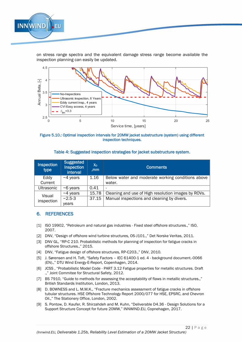
22 | P a g e
(Innwind.EU, Deliverable 1.25b, Reliability Level Estimation of a 20MW Jacket Structure)
on stress range spectra and the equivalent damage stress range become available the
inspection planning can easily be updated.
Figure 5.10.: Optimal inspection intervals for 20MW jacket substructure (system) using different
inspection techniques.
Table 4: Suggested inspection strategies for jacket substructure system.
Inspection
type
Suggested
Inspection
interval
X0
,mm Comments
Eddy
Current
~4 years 1.16 Below water and moderate working conditions above
water.
Ultrasonic ~6 years 0.41 -
Visual
inspection
~4 years 15.78 Cleaning and use of High resolution images by ROVs.
~2.5-3
years
37.15 Manual inspections and cleaning by divers.
6. REFERENCES
[1] ISO 19902, “Petroleum and natural gas industries - Fixed steel offshore structures.,” ISO,
2007.
[2] DNV, “Design of offshore wind turbine structures, OS-J101.,” Det Norske Veritas, 2011.
[3] DNV GL, “RP-C 210. Probabilistic methods for planning of inspection for fatigue cracks in
offshore Structures.,” 2015.
[4] DNV, “Fatigue design of offshore structures, RP-C203.,” DNV, 2010.
[5] J. Sørensen and H. Toft, “Safety Factors – IEC 61400-1 ed. 4 - background document.-0066
(EN).,” DTU Wind Energy-E-Report, Copenhagen, 2014.
[6] JCSS , “Probabilistic Model Code - PART 3.12 Fatigue properties for metallic structures. Draft
.,” Joint Commitee for Structural Safety, 2012.
[7] BS 7910, “Guide to methods for assessing the acceptability of flaws in metallic structures.,”
British Standards Institution, London, 2013.
[8] D. BOWNESS and L. M.M.K., “Fracture mechanics assessment of fatigue cracks in offshore
tubular structures. HSE Offshore Technology Report 2000/077 for HSE, EPSRC, and Chevron
Oil.,” The Stationery Office, London, 2002.
[9] S. Pontow, D. Kaufer, R. Shirzahdeh and M. Kuhn, “Deliverable D4.36 - Design Solutions for a
Support Structure Concept for future 20MW,” INNWIND.EU, Copnehagen, 2017.
23 | P a g e
(Innwind.EU, Deliverable 1.25b, Reliability Level Estimation of a 20MW Jacket Structure)
[10] D. Kaufer, “INNWIND.EU reference jacket 20MW,” Ramboll, Hamburg, 2017.
[11] DNV RP-C203, “Fatigue design of Ofshore steel structures,” Det Norske Veritas, 2014.
[12] DNV-GL, “Recomended Practice RP-0001. Probabilistic methods for planning of inspection for
fatigue cracks in offshore structures,” Det Norske Veritas - GL, 2015.
[13] Lobitz DW, Veers PS, Eisler GR, Laino DJ, Migliore PG, Bir G. The Use of Twist-Coupled Blades
to Enhance the Performance of Horizontal Axis Wind Turbines. Sandia Report SAND 2001-
1303, Sandia National Laboratories, Albuquerque, NM, May 2001..
[14] Lobitz D, Veers PS, Laino D. Performance of twist-coupled blades on variable speed rotors.
AIAA 2000-0062, 2000 ASME Wind Energy Symposium, Reno, January 10–13, 2000..
[15] Bottasso C.L., Campagnolo F., Croce A., “Multi-Disciplinary Constrained Optimization of Wind
Turbines”, Multibody System Dynamics, Vol. 27, N. 1, p. 21-53, 2012, ISSN: 1384-5640, doi:
10.1007/s11044-011-9271-x (2012)..
[16] Bottasso CL, Croce A. Cp-Lambda: User’s Manual. Dipartimento di Ingegneria Aerospaziale,
Politecnico di Milano, 2006–2011..
[17] A.Croce, Deliverable D2_22_PoliMI_16July2015.txt.
[18] Bottasso C.L., Campagnolo F., Croce A., Tibaldi C., “Optimization-based study of bend–twist
coupled rotor blades for passive and integrated passive/active load alleviation”, Wind Energy,
Vol. 16, N.8, p1149-1166, 2013. DOI: 10.1002/we.1543 (2013)..
[19] Zahle, F., Tibaldi, C., Verelst, D. R., Bak, C., Bitche, R., and Blasques, J. P. A. A., Aero-Elastic
Optimization of a 10MW Wind Turbine, Proceedings of the 33rd Wind Energy Symposium ,
Kissimmee, Florida, U.S.A., 2015.
[20] P.K. Chaviaropoulos, J. Beurskens and S.Voutsinas,” Moving towards Large(r) Rotors – Is that
a good idea?”, Proc. EWEA 2013 Conference, Vienna, 2013.
[21] P.K. Chaviaropoulos and G. Sieros, “Design of Low Induction Rotors for use in large offshore
wind farms”, Proc. Scientific Track, EWEA 2014, Barcelona, 2014.
[22] P.K. Chaviaropoulos, G.Sieros, J.M. Prospathopoulos, K. Diakakis and S.G. Voutsinas, “Design
and CFD-based Performance Verification of a Family of Low-Lift Airfoils”, Proc. EWEA 2015,
Paris, 2015.
[23] INNWIND.EU Deliverable 2.14.
[24] P. Bortolotti, C. L. Bottasso and A. Croce, “Combined preliminary-detailed design of wind
turbines,” Wind Energy Science, vol. 1, pp. 71-88, 2016.
[25] INNWIND.EU Deliverable 1.25b.
[26] INNWIND.EU Deliverable 1.25a, 20MW Reference Wind Turbine, Aeroelastic Data of the
Onshore Version.
[27] INNWIND.EU Deliverable 2.12, New Airfoils for High Rotational Speed Wind Turbines, 2015.
[28] INNWIND.EU Deliverable 1.22.
[29] INNWIND.EU Deliverable 1.24.
[30] INNWIND.EU Deliverable 1.23.
[31] IEC 61400-1. Wind turbines – Part 1: Design Requirements, 2005.
[32] INNWIND.EU Deliverable 4.36.
[33] “DNVGL-ST-0126, Support structures for wind turbines, 2016”.
[34] “DNVGL-RP-C203, Fatigue Design of offshore steel structures, 2016”.
[35] J. Serrano-González, “Technological evolution of onshore wind turbines-a market-based
analysis,” Wind Energy, 2016.
[36] W. H. Lio, “Fundamental performance similarities between individual pitch control strategies
for wind turbines,” International Journal of Control, vol. 90, no. 1, 2017.
[37] CDV IEC, “61400-1 ed.4. Wind Turbines - Part 1: Design requirements,” IEC, Geneva, 2017.
24 | P a g e
(Innwind.EU, Deliverable 1.25b, Reliability Level Estimation of a 20MW Jacket Structure)