Embed Size (px)
Citation preview
Aalborg Universitet
Comparing a k- Model and the v2-f Model in a 3D Isothermal Wall Jet
Davidson, Lars; Nielsen, Peter Vilhelm
Publication date:2003
Document VersionPublisher's PDF, also known as Version of record
Link to publication from Aalborg University
Citation for published version (APA):Davidson, L., & Nielsen, P. V. (2003). Comparing a k- Model and the v2-f Model in a 3D Isothermal Wall Jet.Aalborg: Dept. of Building Technology and Structural Engineering, Aalborg University. Indoor EnvironmentalEngineering, No. 50, Vol.. R0301
General rightsCopyright and moral rights for the publications made accessible in the public portal are retained by the authors and/or other copyright ownersand it is a condition of accessing publications that users recognise and abide by the legal requirements associated with these rights.
? Users may download and print one copy of any publication from the public portal for the purpose of private study or research. ? You may not further distribute the material or use it for any profit-making activity or commercial gain ? You may freely distribute the URL identifying the publication in the public portal ?
Take down policyIf you believe that this document breaches copyright please contact us at [email protected] providing details, and we will remove access tothe work immediately and investigate your claim.
Downloaded from vbn.aau.dk on: juni 11, 2018
Comparing a k-£ Model and the V- f Model in a 30 Isothermal Wall Jet
Lars Davidson, Peter V Nielsen
..-0 ("") 0 0::: ("")
lO Ol r--
1 lO Ol ("") ..-z (/) (/)


Comparing a k-E Model l
and the \1- f Model in a
30 Isothermal Wall Jet
Lars Davidson, Peter V. Nielsen


Con1paring a k - c Model and the v2 - f Model in
a 3D Isothermal Wall Jet
'
Lars Davidson* Dept. of Thermo and Fluid Dynamics
Chalmers University of Technology SE-412 96 Goteborg, Sweden
http:/ /www:tfd.chalmers.se/-lada
Peter V. Nielsen Dept .. of Building Technology and Structural Engineering
Aalborg University Sohngaardsholmsvej 57
DK-9000 Aalborg, Denmark http:/ /www.civil.auc.dk/i6/staff/navn/i6pvn.html
1 Abstract
In this work the flows in a three-dimensional wall jet and in a fully developed plane channel"are computed. Two different turbulence models are used, the low-Re k- E model of Abe et al. (1994) and the v2 - f model of Durbin (1991). Two modifications of the v2 - f model are proposed. In the original model the wall-normal stress v2 is allowed to exceed 2k/3, although it is supposed to be the smallest of the normal stresses. A simple modification of the v2 - f model is proposed which takes care of this problem. In the v2 - f model, two velocity scales are available, k112 and ( v2 ) 112 ,
where the latter is the wall-normal fluctuations which are dampened by the wall. In the second modification of the v2 - f model we propose to use two viscosities, one (vt,.d -based on (v2)112 -for the turbulent diffusion in the wall-normal direction, and the other (vt,ll) - based on k112 - for the tmbulent diffusion in the wall-parallel directions.
·Part of this work wa.s carried out during the first author's stay at Dept. of Building Technology and Structural Engineering, AaJborg University in Autumn 2002.
1

2 INTRODUCTION 2
2 Introduction
In rooms ventilated with mixed ventilation the flow is usually supplied through an inlet device mounted on a wall just below the ceiling. The resulting flow is a wall jet developing along the ceiling. The flow in this w·au jet determines the flow in the whole room. Thus it is very important to be able to predict the flow in the wall jet in order to be able to design the yentilation system.
The flow in an isothermal three-dimensional wall jet is the subject of the present work. It is well known that the spreading rates of a wall jet are very different in the wall-normal and the spanwise directions. The reason for the behavior is the presence of the wall which inhibits the turbulence in the wall-normal direction and hence also the spreading. According to the measurement by Abraharnsson et al. (1997), the spreading rates in the wallnorm~! and spanwise direction are dy1; 2/dx = 0.065 and dz1; 2 fdx = 0.32, respectively. The large spreading rate in the spanwise direction is created by a strong secondary motion, generated by the normal stresses (Craft & Launder, 2001), analogous to how secondary motion in a square duct is generated. Whereas the magnitude of secondary motion in a square duct is
1 approximately one percent of the streamwise velocity (Pallares & Davidson, 2000), the secondary motion in a three-dimensional wall jet is much larger. Abrahamsson et al. (1997) report values of up to 18% (scaled with the local streamwise velocity), and predictions employing second-moment closures of Craft & Launder (2001) show spanwise velocities of up to almost 0.3.
In the present study we use a low-Re k- e model (Abe et al., 1994) and the v2 - f model (Durbin, 1991). Two modifications are proposed for the v2 - f ~odel.
1. In the v2 - f model, a transport equation is solved for the wall-normal stress v2 . The idea is to model the reduction of v2 as walls are approached. Thus v2 should be smaller than the other normal stresses, which means that v2 ~ 2k/3 since k = (u2 +v2 +w2)/2. This relation is not satisfied in the standard v2 - f model. In the present work a simple modification is proposed which gives v2 ~ 2k/3 everywhere. The modification is shown to work well in fully developed channel flow and for the 3D wall jet.
2. In the v2 - f model, two turbulent velocity scales are available, ( v2) 112
and k 112 . In eddy-viscosity models - including the v2 - f model -the turbulent diffusion is modelled employing an isotropic turbulent viscosity using one turbulent velocity scale and one turbulent lengthscale. Since in the v2 - f model we have two turbulent velocity scales, the v2 - f model is in the present work modified so that one turbulent viscosity (1/t,J.) - computed with (v2)112 - is used for the turbulent
3 NUMERICAL METHOD 3
Mesh .6.Xmin, .6.Xmax .6.ymin , .6.Ymax tlzmin' tlzmax (Ny,NJin
1 5.4. 10-4 ' 0.14 1.6 . w-4 , o.o45 4.3 . w-·l, o.015 21,9 2 1.62 . w-3, o.o7 1. 7 . w-4 , o.o39 2.1 . w-4 , 0.021 31, 15
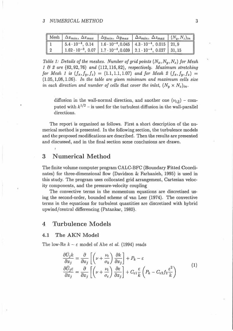
Table 1: Details of the meshes. Number of grid points (Nx, Ny, Nz) for lvfesh 1 F.1 2 are (82, 92, 76) and (112, 116, 82), respectively. Maximum stretching for Mesh 1 is Ux, fy, fz) = (1.1, 1.1, 1.07) and f or lvfesh 2 Ux, fv, f z) = (1.05, 1.08, 1.06). In the table are given minimum and maximum cells size in each direction and number of cells that cover· the inlet, (Ny x Nz)in·
diffusion in the wall-normal direction, and another one (r;t,ll) - com
puted with k112 - is used for the turbulent diffusion in the wall-parallel directions.
The report is organized as follows. First a short description of t he numerical method is presented. In the following section, the turbulence models and the proposed modifications are described. Then the results are presented and discussed, and in the final section some conclusions are drawn.
3 Numerical Method
The finite volume computer program CALC-BFC (Boundary Fitted C oordinates) for three-dimensional flow (Davidson & Farhanieh, 1995) is used in this study. The program uses collocated grid arrangement, Cartesian velocity componen~s, and the pressure-velocity coupling
The convective terms in the momentum equations are discretized using the second-order, bounded scheme of van Leer (1974). The convective terms in the equations for turbulent quantities are discretized with hybrid upwind/central differencing (Patankar, 1980).
4 Turbulence Models
4.1 The AKN Model
The low-Re k - E model of Abe et al. (1994) reads
(1)

4 TURBULENCE ~MODELS
(2)
* UcY ( 1/4 Y = -, UE = El/) l/
Boundary conditions for E at walls is
2vk E=-
y2 (3)
The coefficients are
c~ eEl cc2 O"k Cfc
0.09 1.5 1.9 1.4 1.4
4.2 The v2 - f Model
In the v2 - f model of Durbin (1991, 1993, 1996) two additional equations
are solved: the wall-normal stress v2 and a function f. This is a model which is aimed at improving modelling of the effects of walls on the turbulence. Walls affect the fluctuations in the wall-normal direction v2 in two ways.
1. The wall damping of v2 is felt by the turbulence fairly far from the wall (y+ ;S 200) through the pressure field;
2. Viscous damping takes place within the viscous and buffer layer (y+ ;S 20).
In usual eddy-viscosity models both these effects are accounted for through damping functions. The damping of v2 is in the Reynolds stress models accounted for through the modelled pressure-strain terms q,~2, 1 and q,~2 ,2 .
In the v2 - f model the problem of accounting for the wall damping of v2
is simply resolved by solving the transport equation of v2 . The v2 equation in boundary-layer form reads (Davidson, 2002)
apUv2 apv v2 a [ av2] ax + ay = ay (p. + 1-Lt) ay - 2vapjay- PE22 (4)
in which the diffusion term has been modelled with an eddy-viscosity assumption (Davidson, 1995, 2002). Note that the production term P22 = 0
4 TURBULENCE MODELS 5
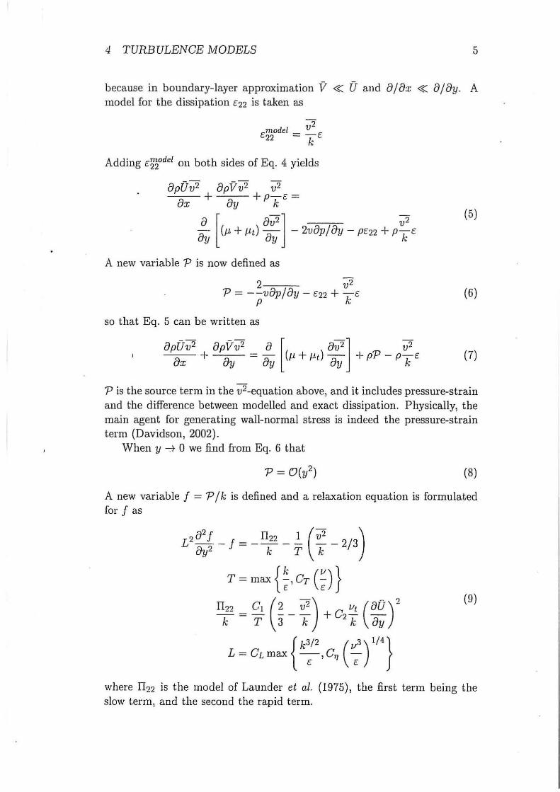
because in boundary-layer approximation V « (J and a;ax « ajay. A model for the dissipation c22 is taken as
v2 [model c
22 = k
Adding t:'!J2odel on both sides of Eq. 4 yields
apuJi apv-:;;'2 v2
ax + ay + p k c =
a [ &v2] v2 ay (J..L + J..Lt) &y - 2vapjay - PE22 + p k c
(5)
A new variable P is now defined as
2 v2
P = --vapjay- E22 + -k c p ~
(6)
so that Eq. 5 can be written as
&p0v2 apVv2 a [ av2] v2
-- + = - (J..L + f..Lt) - +pP - p- E ax ay &y ay k
(7)
P is the source term in the v2-equation above, and it includes pressure-strain and the difference between modelled and exact dissipation. Physically, the main agent for generating wall-normal stress is indeed the pressure-strain term (Davidson, 2002).
When y-:+ 0 we find from Eq. 6 that
(8)
A new variable f = P / k is defined and a relaxation equation is formulated for f as
? a2 f rr22 1 ( v
2 ) L--- f = --- - --2/3
&y2 k T k
T = max { ~ , Cr (;) }
IT22 = C1 (~ _ v2
) + 02 vt (a0) 2
k T 3 k k ay
(9)
L ~CL max { k~2
,C" (:3
)
114
}
where II22 is the model of Launder et al. (1975), the first term being the slow term, and the second the rapid term.

4 TURBULENCE JviODELS
f
2.-----~----~----~---. --~.---..-, +
+
+
1.5 +
+
+
+
0 0 0 0 0 0 0
0.4 0.6 0.8 y
6
Figure· 1: Equation 12 with different L and S. Thin solid line: L = 0.04, S = 1; dashed line: L = 0.08, S = 1; thick solid line: L = 0.12, S = 1; dots: L = 0.2, S = 1; +: L = 0.2, S = 2; o: L = 0.2, S = 0.5.
From Eq. 9 we get that f = O(y0) as y -+ 0, and thus the near-wall behavior of P is enforced. Far from the wall when 82 f / 8y2 ~ 0, Eq. 9 yields
kf = P-+ l122 + c(v2/k- 2/3) (10)
When this expression is inserted in Eq. 7 we get
(11)
which is the usual form of the modelled v2-equation with isotropic dissipation. Thus the f equation acts so as to let f go from its wall value to the value of its source term over scale L. In this way the reduction of P in Eq. 7 as the wall is approached is modelled. The behavior of the equation for f (Eq. 9) for different right-hand sides is illustrated in Fig. 1 where the equation
(12)
has been solved for different L and S. As can be seen f approaches the value of the source term as y > L.
4.3 The v2 - f model if Lien & Kalitzin (2001)
Lien & Kalitzin {2001) proposed a modification of the v2 - f model allowing the simple explicit boundary condition f = 0 at walls. This modified model

4 TURBULENCE MODELS 7
is used in the present work. The v2 and f -equation read (Lien & Kalitzin, 2001)
8U·v2 a [ 8v2] v
2 1 = - (v + vt)- + kf- 6-E ox· ox· ox· k J J J
2 82 f 1 [ v
2 2 ] Pk L -f-- (C1-6)---(C1-1) +C2-=0
8x·8x· T k 3 k J J "----v--'
~-----.,..------- Term 2 Term 1
P ( aui auj) aui
k=Vt -+-- -OX j a.r.i ax j
T = max { ~, 6 ( ~) 112
}
L= CLmax - C -{ k3/2 ( v3)
1/4}
[ ' Tf [
The turbulent viscosity is computed from
(13)
(14)
(15)
The k and c-equations are also solved (without damping functions). Boundary conditions at the walls are
k = v2 = f = 0, E = 2vk/l (16)
The coefficients are given the following values:
CJL CE2 Uk aE c1 c2 CL eT] 0.22 1.9 1 1.3 1.4 0.3 0.23 70
and CE] = 1.4(1 + 0.05(kjv2)lf2 ).
Note that in the v2 - f model v2 denotes a generic wall-normal fluctuation component rather than the fluctuation in the y direction. This is achieved by the source - kf which is the modelled pressure-strain term - which is affected by the closest wall.
4.3.1 Modification I
The source term kf in the v2-equation (Eq. 13) is the modeled pressure strain term which is dampened near walls as f goes to zero. Since v2 represents the wall-normal normal stress, it should be the smallest normal stress, i.e. v2 :::; u2 and v2 :::; w2, and thus v2 should be smaller than ~k since k = (u2 + v2 + w 2 )j2. In the homogeneous region far away from the wall, the

4 TURBULENCE lviODELS 8
Laplace term should be negligible i.e. a2 f I axjaXj -7 0. T hen Eq. 14 reduces to (cf. Eq. 10)
(17)
It turns out that in the region far away from the wall, the Laplace term is n?t negligible, and as a consequence v 2 gets too large so that v2 > ~k . A simple modification is to set an upper bound on the source term kf in the v2-equation as
2 _ . { . 1 [(c )2 2k (C )] } V souTce - nun kj, - T 1 - 6 V - 3 1 - 1 + C2 Pk ' (18)
This modification ensures that v2 ::; 2kj3. In regions where v2 :::: 2k/3, the turbulent viscosity with the v2 - f model is 2 · 0.22k2 /(3£) = 0.147k2 /£ (see Eq. 15) which is considerably larger than the s tandard value in the k - £
model, 0.09k2 j£. A simple remedy is to compute Vt as
(19)
Equations 18 and 19 are called "Modification P', unless otherwise stated.
4.3.2 Modification II
In the v2 - f model we have two velocity time scales, ( v2 ) 112 and k112 . The wall-normal stress v2 is dampened near walls as j goes to zero. Thus it is natmal to introduce two viscosities, one for wall-normal diffusion (vt, .d and one for diffusion parallel to the wall (vt,ll) In the present study, we propose to compute them as
1/t,J. = 0.22v2T, vt,ll = 0.09kT (20)
For a wall parallel to the x - z plane (at y = 0, for example), the turbulent diffusion terms are computed as
a ( ai!?) - VtJ. -ay · ay a ( ai!? )
8xi vt,llaxi ,j =I 2
{21)
where ii? denotes a velocity component. Equation 21 could also be used for the turbulent quantities, but the effect is largest in the momentum equations, and in the present work Eq. 21 is used only in the momentum equations.

5 RESULTS 9
5 Results
5.1 Channel Flow
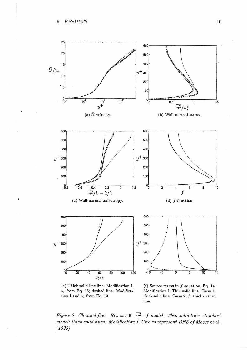
In Fig. 2 channel flow predictions are presented. The computations are carried out as lD simulations, and the Reynolds number based on the friction velocity is ReT = u*8jv = 590, where 8 denotes half-width of the channel. The number of cells used to cover half of the channel is 64, and a geometric stretching factor of 1.08 is used. The node adjacent to the wall is located at y+ = 0.14. The results presented in Fig. 2 have been obtained using the v2 - f model.
From 2a it can be seen that the velocity profile is only very little affected by Modification I. The v2 profile is much better predicted with Modification I, as can be seen from Fig. 2b. Without the modification, v2 becomes too large for y+ > 150, and it is also seen from Fig. 2c that v2 for y+ > 400 erroneously becomes larger than 2k/3.
In Fig. 2d it can be seen that Modification I reduces f . The reason is that we have a positive feedback: the modification reduces v2 by reducing its source (Eq. 18) , which in turn reduces f by reducing part of its source (6- C1)v2 jk, which further reduces the source in the v2 equation and so on.
I
The tmbulent viscosity is presented in Fig. 2e using either Eq. 15 or Eq. 19. It can be seen that switching from the v2 - f expression (Eq. 15) to the k- E expression has only a small effect on the computed Vt. For y+ > · 380 the viscosity from the k - E expression becomes larger than Vt
from the v2 - f model. The effects this switching have on the results in Fig. 2a-d are negligible.
In Fig. 2f the source terms in the f equation are depicted. It can be seen that near the wall Term 2 is largest, and that is because the velocity ao I 8y in the Pk is largest here. Furthermore, it is seen that, overall, the largest contribution is given by -f. The sum of the somce terms- which nowhere goes to zero- is balanced by (1/L2 )82 f j8y2 .
5.2 The Wall Jet
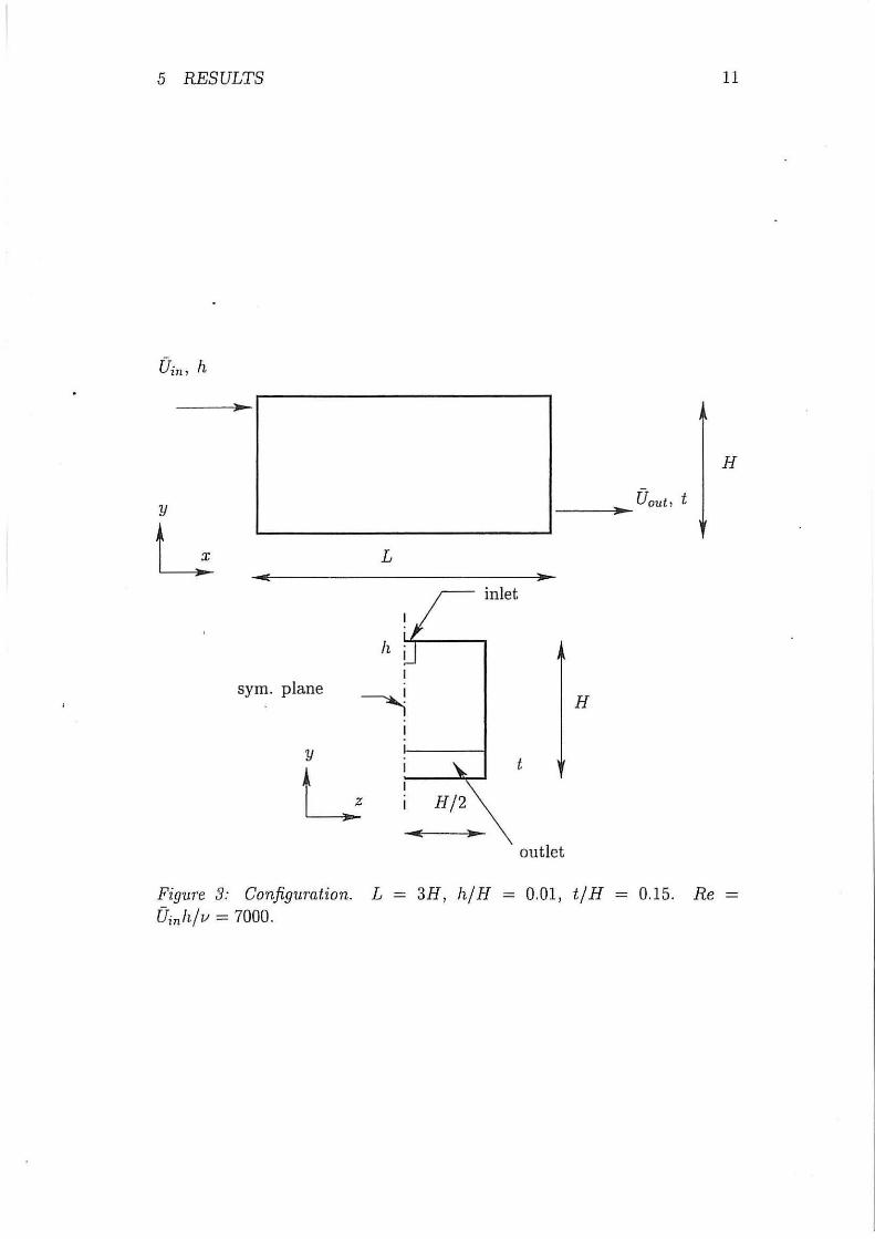
The configuration is shown in Fig. 3. The square inlet is located at the uppermost part of the left wall and the outlet (a slot) is situated at the lowermost part of the right wall. Since the geometry is symmetric only half of the configuration is considered.
In Fig. 4 the y+ values for the nodes adjacent to the walls are depicted. Along the upper wall, y+ is mostly below one (for xj H > 0.5), and the largest values are found along the vertical right wall for which y+ reaches values of approximately 12.
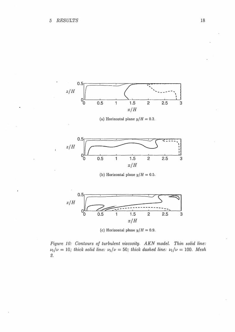
In Figs. 5 - 10 predicted half widths (defined as the position where U(x, y, z ) is half of Umax(x)), horizontal and vertical velocity profiles, U contours and Vt contoms are presented using the AKN model on mesh 1 & 2
5 RESULTS
25
20
15
(J fu* 10
5
0 10- ' 10' 10
2
y+
(a ) 0 -velocity.
600
500
400
y+ 300
200
100
- 8.8 -0.6 - 0.4 -0.2 0 0.2
v2/k- 2/3 (c) Wall-normal anisotropy.
500
400
y + 300
200
40 60 80 100 120
vtfv
(e) Thick solid line line: Modification I, v1 from Eq. 15; dashed line: 1\tlodificat ion I and Vt from Eq. 19.
10
600
500
400
y+ 300
200
100
0 0.5 1.5
v2 fu; (b) Wall-normal s tress ..
600
500
400
y+ 300
200
100
00 2 4 6 8 10
f (d) !-function.
600
500 . . 400
. . . . . y+ 300
. . . . . 200 . . 100 ' .
' ' _qo ----·---
- 5 0 10 15
(f) Source t erms in f equat ion, Eq. 14. Modification I. Thin solid line: Term 1; thick solid line: Term 2; f: thick dashed line.
FiguTe 2: Chann el flow. R e-r = 590 . v2 - f model. Thin solid line: standard model; thick solid lines: Modification I. Circles represent DNS of Maser et al. (19.99}
5 RESULTS
y
G L
h
sym. plane
y
L Figure 3: Configuration. L
Uinh/v = 7000.
11
H
inlet
H
t
outlet
3H, h/H = 0.01, tjH 0.15. Re

5 RESULTS
12
10
8
y+ 5
· 4
2
(a) Mesh 1.
12
10
8
5
8 2 4 s
(b) Mesh 2.
12
Figure 4: y+ joT the neaT-wall nodes along the perimeter of the domain. AKN model. z = 0. 0 :::; s :::; 3: wall at y = H; 3 :::; s :::; 4: wall at x = L; 4 :::; s :::; 7: wall at y = 0; 7 :::; s :::; 8: wall at x = 0. Dashed lines indicates where the walls start and end.
are shown. It can be seen that the results are fairly grid independent. The spreading rates dfJ1;2/ dx and dz1; 2 /dx are both close to 0.065. This is in disagreement with experiment from where it is known that the spreading rate in the wall-normal direction (y) is much smaller than the one in the spanwise direction (z). The reason is that the turbulence in the wall-normal direction is dampened by the wall. The experimental values are df11;2/ dx = 0.065 and dz1; 2 / dx = 0.32 according to the measurement by Abrahamsson et al. (1997).
The predicted spreading f11;2 and z1; 2 , contours of U and Vt in Figs. 11-16
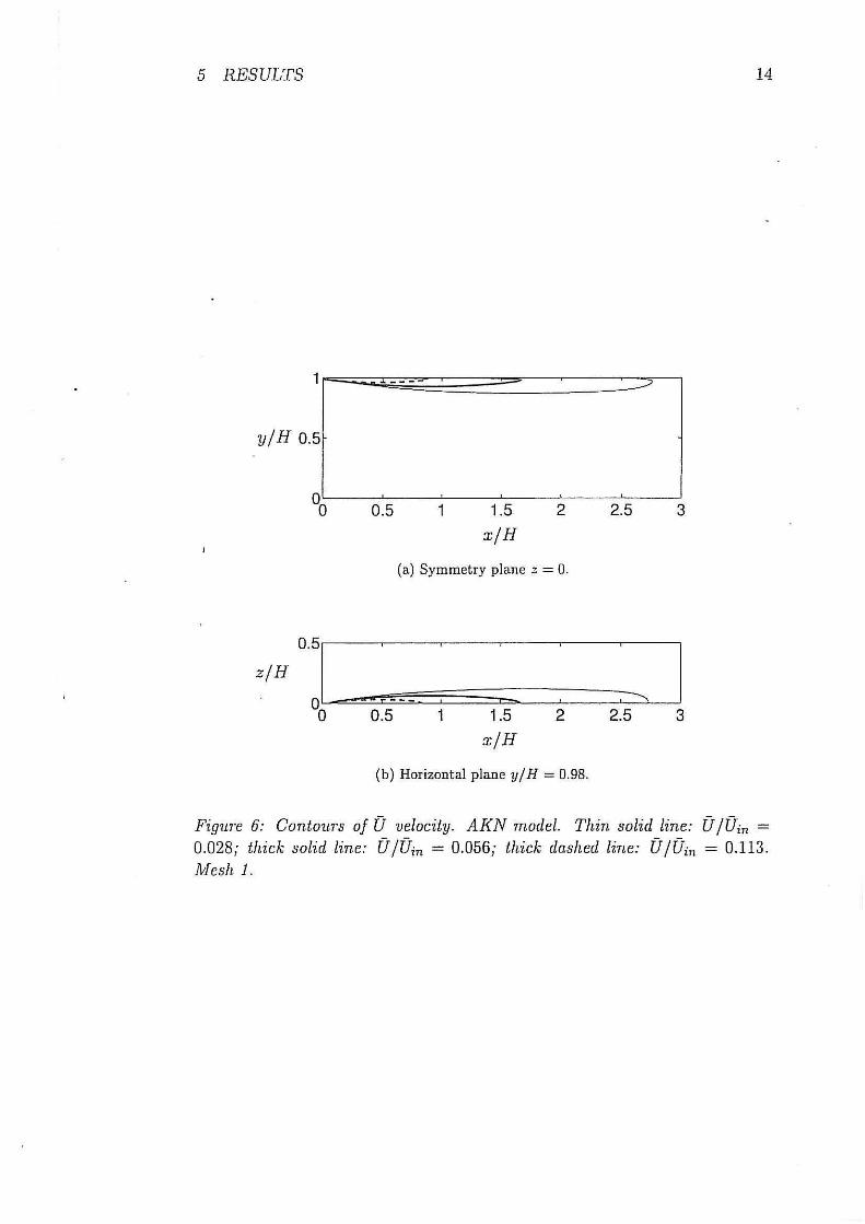
using the v2 - f model show that the predictions are fairly grid-independent. Comparing '[;1; 2 and z1; 2 with the corresponding predictions with the AKN model in Figs. 5 and 8 it can be seen that, as expected, the predicted spreading of the wall jet is larger with the AKN model than with the v2 - f model. The reason is that the wall-normal stress v2 in the v2 - f model is dampened by the reduced f as the wall is approached. When v2 is reduced, so is also the turbulent viscosity and thereby also the entrainment. The reduced entrainment results in higher streamwise velocity, which can be seen by comparing Figs. 12 and 15 with Figs. 6 and 9
In Figs. 17 and 18 the effect of Modification I is investigated. It can be seen from Fig. 17 that without Modification I the predicted v2 becomes much larger than 2kj3, which is physically incorrect. However, with Modification I, v2 :::; 2k/3 as required. It can be noted that the effect on f is hardly noticeable (cf. Figs. 17c and Figs. 17d). As v2 is over-predicted, this also

5 RESULTS
0.25r--~-~-~--..--~--.
::r:: 0.2 ......_ C'l ......... N' o.15
::r:: 0.1 ......_ N .........
.;;; 0.05
00~-~-~-~---~-~-~
0.5 1.5 2 2.5 3
x/H
(a) ;rhin solid line: fj1; 2 ; dashed line: z1; 2 ; thick solid line: 0.065x.
2
1.5
N ......... ...... N ......_ N
0.5
0.5
0.2 0.4 0.6 0.8
[! /Umax (b) Vertical velocity profile.
0.2 0.4 0.6 0.8
[! /Umax (c) Horizontal velocity profile.
13
1.2
Figure 5: Spreading of the wall jet; vertical and horizontal velocity profiles between x/ H = 0.34 and x/ H = 1.07. y = H- y. AKN model. !11esh 1.
5 RESULTS
y/H 0.5
0.5 1 1.5
x/H
2
(a) Symmetry plane z = 0.
zfH OJ ~ .: ___ •
·~ 0 0.5 1 1.5 2 x/H
(b) Horizontal plane y/H = 0.98.
14
2.5 3
: I 2.5 3
Fign1·e 6: Contours of U velocity. AKN model. Thin solid line: U /Uin = 0.028; thick solid line: U /fhn = 0.056; thick dashed line: U /Uin = 0.113. lvfesh 1.

5 RESULTS
1.5 xjH
2
(a} Horizontal plane 11/ H = 0.2 .
2.5 3
• z/H 01 c: ~ ;]11 0 0.5 1.5 2 2.5 3
xjH
(b) Horizontal plane y/H = 0.5.
z/H
0
]~ __ : ____ :: __ ?1 0 0.5 1.5 2 2.5 3
xjH
(c) Horizontal plane yfH = 0.9.
15
FiguTe 7: Contom·s of turbulent viscosity. AKN model. Thin solid line: vtfv = 10; thick solid line: vtfv = 50; thick dashed line: vtfl/ = 100. M esh 1.

5 RESULTS
0.25r--~-~--~--..---~--,
t:q 0.2 -.......
C'l -N' o.15
t:q 0.1 -.......
C'l -I ~ 0.05_;/.·'
N -...... 1.5
I~ 1 -....... I~
0.5
16
oo· 0.5 1.5 2 2.5 3 %'~--0~.2~~0~.4--~0.~6==~0~.8==~--~1.2
xjH [J /Umax (a) Thin solid line: fi1; 2 ; dashed line: z 1; 2 ; thick solid line: 0.065x.
(b) Vertical velocity profile.
2
1.5
N -.-. N -....... N
0.5
%~--~0.-2---0~.4~-0~.6--0~.8~-l--
[J /Umax (c) Horizontal velocity profile.
FiguTe 8: Spreading of the wall jet; vertical and horizontal velocity pTofiles between x/ H = 0.3 and x / H = 1.8. y = H- y . AI<N model. Nfesh 2.

5 RESULTS
yjH 0.5
0.5 1 1.5
x/H
2
(a) Symmetry plane z = 0.
2.5 3
z/H OJ .:___ : : : : I 0 0.5 1.5 2 2.5 3
xjH
(b) Horizontal plane yf H = 0.98.
17
Figure 9: ContouTs of (J velocity. AKN model. Thin solid line: (J /Uin = 0.028; thick solid line: U /Uin = 0.056; thick dashed line: U /Uin = 0.113 . . Mesh 2.
5 RESULTS
1 1.5
x /H
2
(a) Horizontal plane y/ H = 0.2.
2.5 3
z/H ale-: ~ ~-----11 0 0.5 1 1.5 2 2.5 3
x/H
(b) Horizontal plane y/ H = 0.5.
z/H
0);= ;:::;_:------~~_?_:_~~ 0 0.5 1 1.5 2 2.5 3
x/H
(c) Horizontal plane y/ H = 0.9.
18
Figure 10: Contours of turbulent viscosity. AI<N model. Thin solid line: vtfr/ = 10; thick solid line: vtfv = 50; thick dashed line: vtfv = 100. Mesh 2.

5 RESULTS
0.2.----~-~-~--~-~--.
::t: ........... 0.15 N ........ ..... N
0.1
N
::::;- 0.05 ~~
0.5 1.5 2 2.5
x/H
(a) Thin solid line: ii1; 2 ; dashed line: z1
1; 2 ; thick solid line: 0.065x.
2
1.5
N ........ ...... N
........... N
0.5
3
C'l ........
2
1.5
I;;; 1 ........... ~~
0.5
0.2 0.4 0.6 0.8
(j /Umax (b) Vertical velocity profile.
0.2 0.4 0.6 0.8
[J /Umax (c) Horizontal velocity profile.
19
1.2
Figure 11: Spreading of the wall jet; vertical and horizontal velocity profiles between xj H = 0.3 and xj H = 1.8. fj = H- y. v2 - J model, Modification I. Mesh 1.
5 RESULTS
y/H 0.5
0.5 1.5
x/H
2
(a) Symmetry plane z = 0.
2.5 3
z/H 0.:01~:. ____ ~~--.~.~~ .~~I 0.5 1 1.5 2 2.5 3
x/H
(b) Horizontal plane y / H = 0.98.
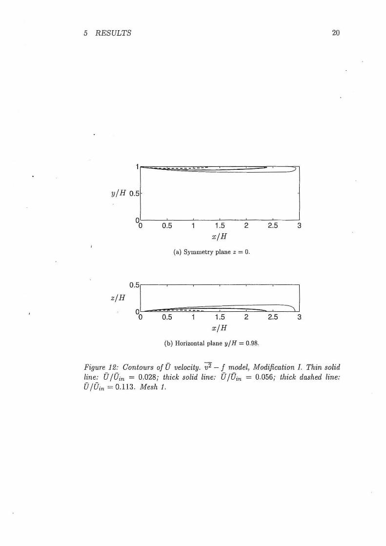
20
FiguTe 12: Contours of [J velocity. v2 - f model, Modification I. Thin solid line: U /Uin = 0.028; thick solid line: U /Uin = 0.056; thick dashed line: U /Uin = 0.11 3. Mesh 1.
5 RESULTS
zjH 0.51( ' : ' 2:J %~---0~.5----~1----~1.~5--~2~---2~.5----~3
x/H
(a) Horizontal plane y/H = 0.2.
zjH ol , :z == :s:J 00~--~----~L---~--~----~----~
0.5 1 1.5 2 2.5 3
x/H
(b) Horizontal plane y/ H = 0.5.
zjH OJc : ::;;; ___ :=;_: __ j 0 0.5 1 1.5 2 2.5 3
x/H
(c) Horizontal plane y/H = 0.9.
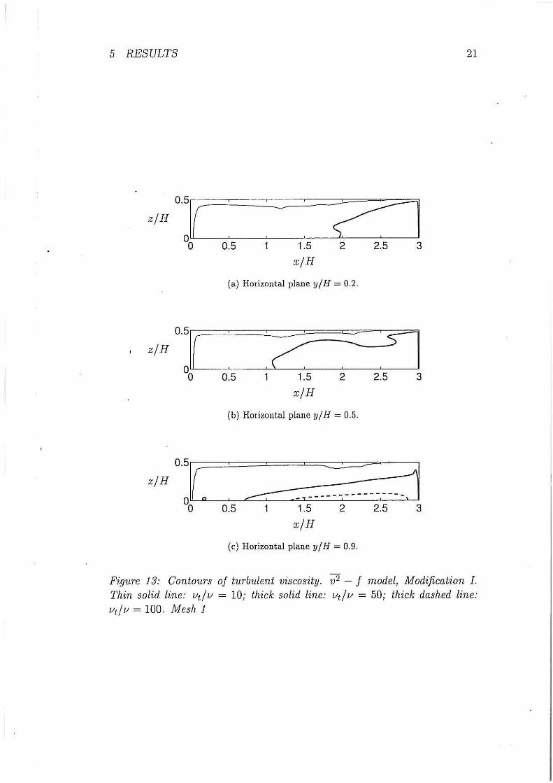
21
Figure 13: Contml1·s of turbulent viscosity. v2 - f model, 111[ odification I. Thin solid line: vtf v = 10; thick solid line: vt/ v = 50; thick dashed line:
vtfz/ = 100. Mesh 1
5 RESULTS
0.2.---~---.--~--~--.----,
~0. 1 5 N ....... .... N
tt:: ........_ N
0.1
::::;- 0.05 1;_::))
22
2
1.5
0.5
OOL--~-~-~--~-~-~ 0.5 1.5 2 2.5 3
oOL----------======c===~--~ 0.2 0.4 0.6 0.8 1.2
xjH (J /Umax (a) Thin solid line: f1 1; 2 ; dashed line: i 11 2 ; thick solid line: 0.065x.
(b) Vertical velocity profile.
2
1.5
N ....... -N ........_ N
0.5
0.2 0.4 0.6 0.8
(J /Umax (c) Horizontal velocity profile.
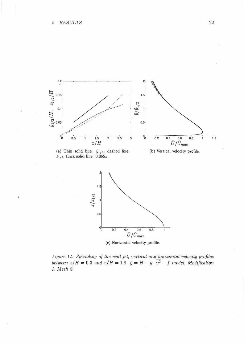
Figu1·e 14: Spreading of the wall jet; vertical and horizontal velocity profiles between x/ H = 0.3 and x/ H = 1.8. y = H- y. v2 - f model, l\1odification I. Mesh 2.

5 RESULTS
yjH 0.5
0.5 1.5
xjH 2
(a) Symmetry plane z = 0.
z fH
0
]: .. ____ :__ •
0 0.5 1.5 2
xjH
(b) Horizontal plane yj H = 0.98 .
23
2.5 3
~ 2.5 3
Figure 15: Contours of 0 velocity. v2 - J model. Thin solid line: 0 jOin = 0.028; thick solid line: 0 jOin = 0.056; thick dashed line: [J jOin = 0.113. Mesh 2.

5 RESULTS
zf H 0.51"---C '---------': '--':..__.___.c:?:~l 0o 0.5 1 1.5
xjH 2
(a) Horizontal plane y/H = 0.2.
2.5 3
z/ H 0 :ll--'"---1( ( ._____.. ..___·,_____,~'------''-----'! 0 0.5 1.5 2 2.5 3
x jH
(b) Horizontal plane y/H = 0.5.
1 1.5
xjH 2
(c) Horizontal plane yjH = 0.9.
2.5 3
24
FiguTe 16: ContouTs of tuTbulent viscosity. v2 - f model, Modification I. Thin solid line: vtfv = 10; thick solid line: vtfv = 50; thick dashed line: vtfv = 100. lvfesh 2.

5 RESULTS 25
0.8 0.8
0.6 0.6
yjH y/H 0.4 0.4
0.2 0.2
o~~----~o----~0.~5----~~ o~~----~------~----~-' 0 0.5
v2 /k-2/3 v2 /k- 2/ 3 (a) Standard v 2 - J model. (b) v2 - f model, Modification I.
1 , .......-'.
O.Br 0.8
0.6 0.6
yjH I yjH 0.4 0.4
0.2 0.2
20 40 60 80 1 00 120 %~~270 --~4~0 --~670---~80~~10~0 --~120
f f (c) Standard v 2 - J model. (d) v2 - J model, Modification I.
0.8
0.6
y/H yjH 0.4
0.2
5 00~~~~~--~--~--~~
0.2 0.4 0.6 0.8 1.2
0.22v2 /0.09/;; 0.22v2j0.09k
(e) Standard v2 - f model. (f) v2 - f model, Modifica tion I.
Figure 17: Pmfiles of (v2 jk- 2/3) and f between xjH = 0.34 and xj H = 1.07. Thin solid line: xj H = 0.34; thick dashed line: x j H = 1.07. Comparison between standard v2 - f model and Modifica tion I. Mesh 1.

6 CONCLUSIONS 26
gives an over-predicted turbulent viscosity compared with a k - £ model. The ratio of these two viscosities, 0.22v2 /(0.09k) (See Eq. 19), is shown in Fig. 17e and f. As can be seen, Vt is over-predicted with up to a factor of four in the outer shear layer of the wall jet compared with a k - £ model. Please recall that in Modification I Vt is computed from Eq. 19.
In Craft & Launder (2001) it was shown that the reason why the spreading rate in the lateral ( z) direction is much larger than that in the wallnor.mal direction (y) is due to a strong secondary motion in they- z plane, driven by the anisotropy in the normal stresses. Thus a Reynolds stress model is required to predict this flow in a proper way. One way to create anisotropic normal stresses in an eddy-viscosity model is to use anisotropic turbulent viscosities.
Below results using the v2 - f model with anisotropic turbulent viscosities are presented. In Figs. 19-21 the predicted thickness of the wall jet, velocity profiles ~nd profiles are depicted for Modification I and II. In Modification II different viscosities are used for the diffusion terms in the wall-normal direction (1.1t,.d and in the wall-parallel direction (vt,ll). The viscosity in
the wall-normal direction is taken from the v2 - f model and the viscosity in the wall-parallel direction is computed with the k- £ expression. The ratio between these viscosities is Vt,J./vt.ll = 0.22v2 /(0.09k), see Eq. 20. The expected effect is that the spreading of the wall jet in the spanwise direction with this modification should be larger than with Modification I. Comparing Figs. 19 and 14 we find that this is indeed the case. Actually the spreading in the wall-normal direction has also increased somewhat, but clearly z1; 2 /f;1; 2
is larger in Fig. 19 than in Fig. 14. Also by comparing the isoline of [J in Figs. 20 a!ld 15 it can be seen that the spreading with Modification I+II is larger than with Modification I.
The ratio Vt,.dvt,ll is shown in Fig. 21, both as profiles and as contours of isolines. It can be seen that Vt,J. is much smaller than Vt,ll· The ratio Vt,.L! Vt,ll
is approximately 0.6 at the location of the velocity peak (f; /f;1; 2 ~ 0.15, see
Fig. 19a). Inside the velocity peak the ratio goes to zero as v2 is dampened by wall (f -t 0).
6 Conclusions
Two modifications of the v2 - f model have been presented. In the first modification - Modification I - the source term in the v2 equation is limited so as to ensure that v2 < 2k/3. The second modification- Modification II - is based on a non-isotropic eddy-viscosity approach. Different viscosities are used for the turbulent diffusion in the wall-normal direction and in the wall-parallel direction. The object of Modification II was to be able to model the different spreading rates in the wall-normal and spanwise direction of a 3D wall jet.

6 CONCLUSIONS
0.5 1 1.5
xjH 2 2.5
(a) Standard v2 - J model. yf H = 0.98
zjH0
J~ :~: 0 0.5 1 1.5 2 2.5
xjH
(b) Standard v2 - J model. z = 0
0.5 1.5
xjH 2 2.5
(c) v2 - j model, Modification I. yf H = 0.98
1.5
x/H
2
(d) v2 - j model, Modification I. z = 0
2.5
27
3
3
3
3
Figure 18: Contour lines ofv2 jk-2/3. Thin solid lines: v 2 jk-2/3 = -0.3 ; thick solid lines: v2 /k - 2/3 = -0.1; thin dashed lines: v2 / k - 2/3 = 0. Comparison between standard v 2 - f model and modified v2 - f model in which source term in v2 equation was limited. Mesh 1.

6 CONCLUSIONS
0.2,.----~-~-~-~-~----.,
,'
tr:: ........... 0.15 ,'
0.1
tr:: ...........
N ::::-0.05
·~
N -......
2
1.5
I;:;; 1 ........... ·~
0.5
28
0.5 1.5 2 2.5 3 ooL-~~--~==~==~==~--7
0.2 0.4 0.6 0.8 1.2
x/H (J /Umax (a) Thin solid line: f11; 2 ; dashed line: z1; 2 ; thick solid line: 0.065x .
(b) Vertical velocity profile.
2
1.5
0.5
%~--o~.2~~o~.4--0~.6~-o~.B-~-
[J /Umax (c) Horizontal velocity profile.
Figm·e 19: Spreading of the wall jet; vertical and horizontal velocity profiles between xj H = 0.3 and xj H = 1.8. y = H- y. v2 - f model, Modification I and I!. 111 esh 2.

6 CONCLUSIONS
y/H 0.5
0.5 1 1.5
x/H
2
(a) Symmetry plane z = 0.
2.5 3
z/H
0
] : ______ :_ : = ; ~ 0 0.5 1 1.5 2 2.5 3
x/H
(b) Horizontal plane y / H = 0.98.
29
Figure 20: Contours of [J velocity. v 2 - f model, Modification I and I!. Thin solid line: U /Uin = 0.028; thick solid line: U /Uin = 0.056; thick dashed line: U /Uin = 0.113. Mesh 2.

6 CONCLUSIONS 30
0.8 1.5
0.6 yjH .
0.4
0.5 0.2
%~~~0~.2--~0~.4--~0~.6---0~.8
Vt, .L/ Vt,ii 1.2 %~~o=.2==~o=.4=-~o~.6---o~.8--~--_j1.2
Vt,J../Vt, ll
(a) Profiles between xj H = 0.34 and x/H = 1.07.
(b) Profiles between x/H = 0.34 and xj H = 1.07. y = H - y.
1 -~-:..----, .. ) -------- ----
yf H 0.5 (----- ---------- __ -::.
0.5 1.5
xjH 2 2.5 3
(c) Isolines of I/t ,J./Vt,ll · y/H = 0.98. Thin solid lines: 0.5; thick solid lines: 0. 7; thin dashed lines: 0.9.
z/H O.:r Sii.z: . 0 0.5 1 1.5 2 2.5 3
xjH
(d) Isolines of vufvt.ll· Thin solid lines: 0.5 ; thick solid lines: 0.7; thin dashed lines: 0.9.
Figure 21: v 2 - f model, Modification I and II. Mesh 2. Vt, .L /vt,ll
REFERENCES 31
Modification I was shown to work well. The predicted v2 was smaller than 2k/3 both for the fully developed channel flow and the 3D wall jet. Modification II was found to give only a small improvement for the 3D wall jet, and with this modification the spanwise spreading rate was increased.
References
ABE,· K., KONDOH, T. & NAGANO, Y. 1994 A new turbulence model for predicting fluid flow and heat transfer in separating and reattaching flows - 1. Flow field calculations. Int. J. Heat Jv! ass Transfer 3 7, 139- 151.
ABRAHAMSSON, H., JOHANSSON, B. & LOFDAHL, L. 1997 The turbulence field of a fully developed three-dimensional wall jet. Report 97/1. Dept. ofThermo and Fluid Dynamics, Chalmers University of Technology, Gothenhurg.
CRAFT, T. & LAUNDER, B. 2001 On the spreading mechanism of the threedimensional turbulent wall jet. Journal of Fluid Mechanics 435, 305-326.
DAV1IDSON, L. 1995 Prediction of the flow around an airfoil using a Reynolds stress transport model. AS.ME: Journal of Fluids Engineering 117, 50-57.
DAVIDSON, L. 2002 MTF270 turbulence modelling. Lecture notes, w'ww.tfd.chalmers.se/doctjcomp_turb_model/, Dept. of Thermo and Fluid Dynamics, Chalmers University of Technology, Goteborg, Sweden.
DAVIDSON, L . & FARHANIEH, B. 1995 CALC-BFC: A finite-volume code employing collocated variable arrangement and cartesian velocity components for computation of fluid flow and heat transfer in complex threedimensional geometries. Rept. 95/11. Dept. of Thermo and Fluid Dynamics, Chalmers University of Technology, Gothenburg.
DuR.BIN, P. 1991 Near-wall turbulence closure modeling without damping functions. Theoretical and Computational Fluid Dynamics 3, 1-13.
DUR.BIN, P. 1993 Application of a near-wall turbulence model to boundary layers and heat transfer. International Journal of Heat and Fluid Flow 14 ( 4), 316- 323.
DuR.BIN, P. 1996 On the k - 3 stagnation point anomaly. International Journal of Heat and Fluid Flow 17, 89-90.
LAUNDER, B. , REECE, G. & Rom, W. 1975 Progress in the development of a Reynolds-stress turbulence closure. Journal of Fluid Mechanics 68 (3), 537-566.

REFERENCES 32
VAN LEER, B. 1974 Towards the ultimate conservative difference scheme. Monotonicity and conservation combined in a second order scheme. Journal of Computational Physics 14, 361-370.
LIEN, F.-S. & KALITZIN, G. 2001 Computations of transonic flow with. the v2f turbulence model. International Journal of Heat and Fluid Flow 22 (1), 53-61.
MOSER, R., KIM, J. & MANSOUR, N. 1999 Direct numerical simulation of turbulent channel flow up to Re7 = 590. Physics of Fluids A 11, 943-945.
PALLARES, J. & DAVIDSON, L. 2000 Large-eddy simulations of turbulent flows in stationary and rotating channels and in a stationary square duct. Report 00/03. Dept. of Thermo and Fluid Dynamics, Chalmers University of Technology.
PATANKAR, S. 1980 Nurne1·ical Heat Transje1' and Fluid Flow. New York: McGraw-Hill.


ISSN 1395-7953 R0301 Printed at Aalborg University
Dept. of Building Technology and Structural Engineering
Aalborg University, January 2003
Sohngaardsholmsvej 57, DK-9000 Aalborg , Denmark
Phone: +45 9635 8080 Fax: +45 9814 8243
http://www.civil.auc.dk/i6