Embed Size (px)
DESCRIPTION
Aadnoy 1998
Citation preview
m*....Society of Petroleum Engineers
iADC/SPE 39391
Friction Analysis for Long-Reach WellsB.S. Aadnoy, Stavanger U., and Ketil Andersen,* Statoil
●IADCMember
Copyright 1998, lADC/SPE Drilling Conference
This paper wss prepared for presentation at the 1998 lADC/SPE Drilling Conference held inDallas, Texss 3-6 Msrch 199B,
~is psper MS selected for presentation by an lADC/SPE Program Comtittee followingreview of information contained In an abstrsct submitted by the author(s). Contents of thepaper, as presented, have not been reviewed by the International Association of DrillingContractors or the Society of Petroleum En~ineers and are subpct to correction by theauthor(s). The material, as presented, does not necessarily reflect any position of the IAM. orSPE, their officers, or members. Papers presented at the lADC/SPE meetings are subject topublication review by Editorial Committees of the IADC and SPE. Electronic reproduction,distribution, or storage of any pert of this paper for commercial purposes without the writtenconsent of the Society of Petroleum Engineers Is prohibited. Permission to reproduce in printia restricted to an abstract of not more than 300 word% illustrations may not be copied. Theabstract must contain conspicuous acknowledgment of tiere and by whom the paper waspresented. Write Librarian, SPE, PO. Box 833636, Richardson, TX 75083-3836, U. S. A., fax01-972-952-9435.
Abstract
Presently wells are drilled in the North Sea approaching ahorizontal reach of 8 km. Plans for the near future is to extendthese towards and beyond 12 km. Well friction is one of themost important limiting factors in this process.
Torque and drag prognosis are today developed on in-housesimulators. Although a good tool for planning, improvementsare made on an trial and error basis, and, these simulators havelimited availability. To provide more insight into the frictionalaspect, a larger study was undertaken. Explicit analyticalequations are derived to model drill string tension for hoistingor lowering of the drill string. The equations are developed forstraight sections, build-up sections, drop-off sections and sidebends. Both constant curvature models and a new modifiedcatenary model are derived. The new catenary model isdeveloped for arbitrary entry and exit inclinations. Equationsto determine well friction in fully 3-dimensional well profilesare also given. Furthermore, based on the tension equations,expressions for torque and drag are developed. Equations forcombined motion and drilling with motor are also given.Using these equations, the total friction in a well is given bythe sum of the contributions from each hole section.
A field study offshore Norway is included in the paper. Usingthe equations derived in the paper, the well path is chosen tominimize the torque on the rig, which is the limiting factor.The paper also summarize a number of guidelines forextended-reach WC1ldesign, and shows the design of an ultra-reach well of more than 12 km reach.
Introduction
The oil industry is in general producing the easiest accessibleoil first, as it gives best economy. However, as existing fieldsare being produced, it becomes important to drain these in anoptimum way. The drilling technology plays an important rolehere as the horizontal reach is more than doubled during thelast decade.
It has become evident that well friction is a limiting factor inextended-reach drilling. Sheppard et.al.’ showed that anundersection trajectory can have reduced drag compared to aconventional tangent section. Banks et.al.2 gives a summary ofextended-reach capabilities. McC1endon and Anders3 studiedthe catenary well profile and demonstrated advantage overconventional methods. The driving force for this developmentwas the need for longer wells.
In Norway this development became very important not onlyto drain older fields more efficiently, but to reduce the numberof offshore platforms on new development projects. Eek-Olsen et. al.4’5and Alfsen et. al.6 demonstrates the evolutionfrom a 3 km reach to more than 7 km horizontal reach. Justadet.al.7 show the planning and drilling of a complex long reachdesigner horizontal well to develop marginal satellite fieldsfrom an existing platform, while Blikra et.al.8 addresses boththe achievements and the cost-benefits. Benesch et. al.’0addresses an extended reach well in Japan.
Aarrestad and Blikra9 gives a good review of the variousaspects of torque and drag problems encountered in extepded-reach drilling. A good, but more general review is given byPayne et. al.lO.
Gou and Miska’2 and Wiggins et.al.’3 defines equations tocalculate the well trajectory. When the well trajectory hasbeen determined, the complete well must be designed. Arecent review over design considerations and potentialproblems is given by Guild et. al.”, while Aadn@y’5 describesthe complete well design process. Sheppard, Wick andBurgess’ formulated the torque and drag models that areimplemented in most simulators.
819
— .
2 B. S. AADNOY AND K. ANDERSEN lADC/SPE 39391
This paper will focus on the planning of the well path.Previous approaches used numerical simulators to plan thewell. In this paper analytical expressions for build, drop, holdand side profiles are derived, and also a new modified catenaryprofile. Using these equations a friction analysis can becarried out without requiring a simulator.
Torque and drag models
Applications. The drag and torque solutions presented beloware derived independently. Therefore their applications are asfollows.
The drag equations applies when tripping in or out of thewell. This may also apply to coiled tubing, logging,completion or workover operations. The torque equationsapplies to pure rotation while drilling. The equation governingcombined motion, both axial movement and rotation, is alsogiven. Reaming, for example, can therefore also be modeled.
The buoyancy factor given in Eqn. 5 is valid if the mud densityin the annulus is equal to the mud density inside the drillpipe.If this is not the case, corrections must be applied.
The paper use the models to analyze the drilling phase of thewell. However, the equations are valid for other phases as wellcompletions, provided a correct scenario is defined.
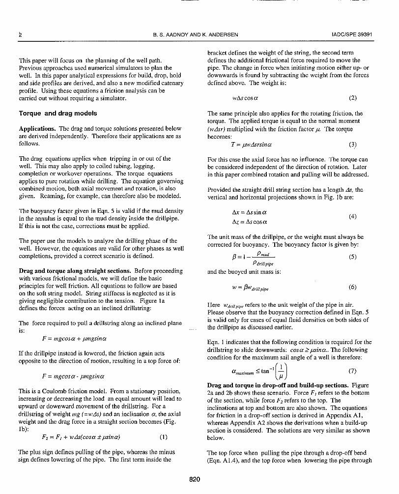
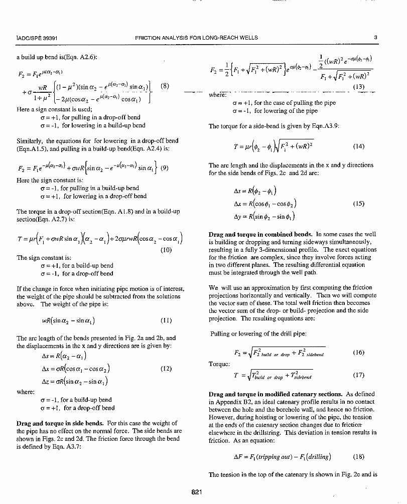
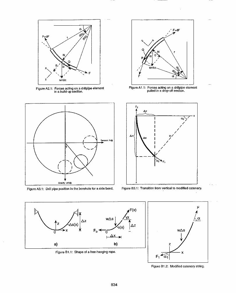
Drag and torque along straight sections. Before proceedingwith various frictional models, we will define the basicprinciples for well friction. All equations to follow are basedon the soft string model. String stiffness is neglected as it isgiving negligible contribution to the tension. Figure ladefines the forces acting on an inclined drillstring:
The force required to pull a drillstring along an inclined planeis:
F = rngcosa + ptngsina
If the drillpipe instead is lowered, the friction again actsopposite to the direction of motion, resulting in a top force of
F = rngcosa - ptlgsin a
This is a Coulomb friction model. From a stationary position,increasing or decreasing the load an equal amount will lead toupward or downward movement of the drillstring. For adrillstring of weight nlg (=w4) and an inclination a, the axialweight and the drag force in a straight section becomes (Fig.lb):
F2 = F1 + vtIAs(coscY &pina) (1)
The plus sign defines pulling of the pipe, whereas the minussign defines lowering of the pipe. The first term inside the
bracket defines the weight of the string, the second termdefines the additional frictional force required to move thepipe. The change in force when initiating motion either up- ordownwards is found by subtracting the weight from the forcesdefined above. The weight is:
WASCOS a (2)
The same principle also applies for the rotating friction, thetorque. The applied torque is equal to the normal moment
(wAsr) multiplied with the friction factor A The torquebecomes:
T = ,uwAsrsina (3)
For this case the axial force has no influence. The torque canbe considered independent of the direction of rotation. Laterin this paper combined rotation and pulling will be addressed.
Provided the straight drill string section has a length A, thevertical and horizontal projections shown in Fig. 1b are:
Ax= Assina
Az=Ascosa(4)
The unit mass of the drillpipe, or the weight must always becorrected for buoyancy. The buoyancy factor is given by:
@=~_ Pm~~ (5)Pdrillpipt.
and the buoyed unit mass is:
w = Pwdrillpipe (6)
Here wdri//pip?refers to the unit weight of the pipe in air.Please observe that the buoyancy correction defined in Eqn. 5is valid only for cases of equal fluid densities on both sides ofthe drillpipe as discussed earlier.
Eqn. 1 indicates that the following condition is required for thedrillstring to slide downwards: cosa >pina.. The followingcondition for the maximum sail angle of a well is therefore:
(7)
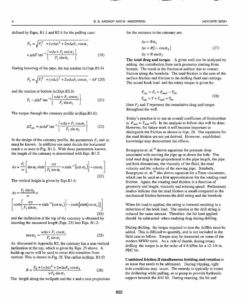
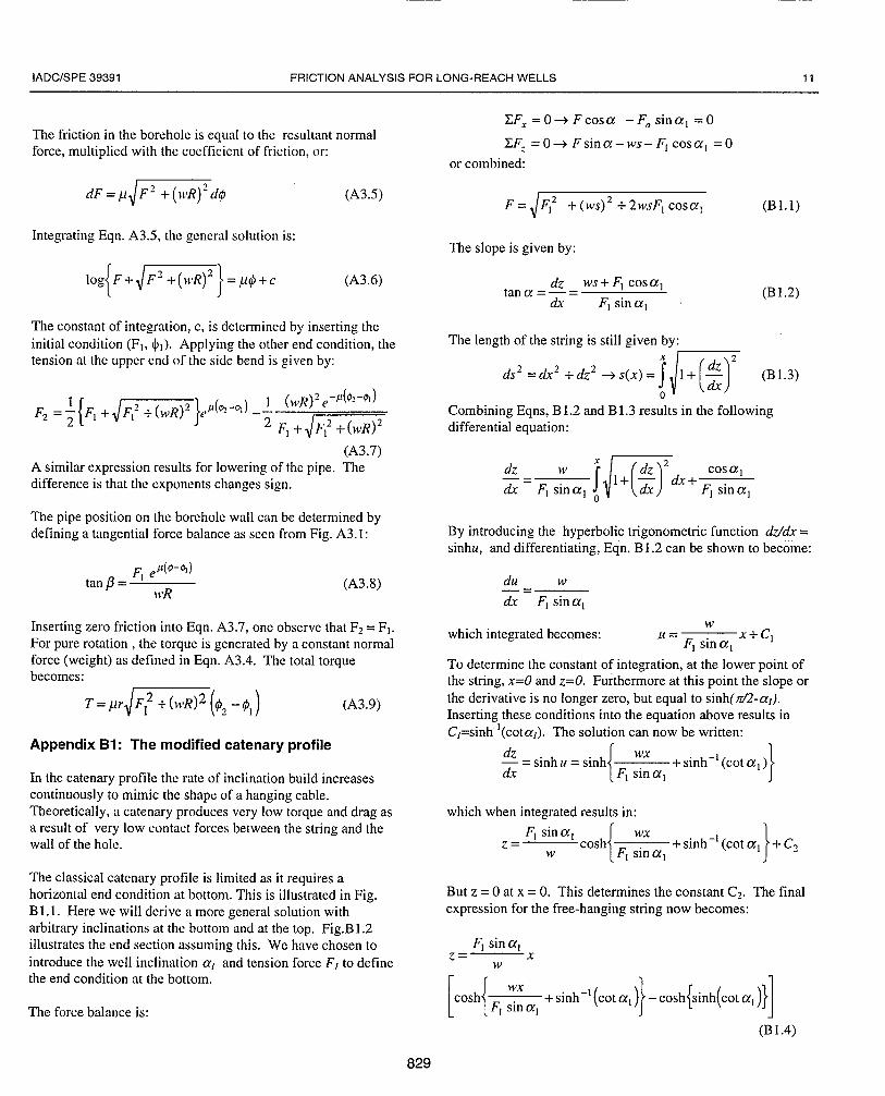
Drag and torque in drop-off and build-up sections. Figure2a and 2b shows these scenario. Force F, refers to the bottomof the section, while force F2 refers to the top. Theinclinations at top and bottom are also shown. The equationsfor friction in a drop-off section is derived in Appendix Al,whereas Appendix A2 shows the derivations when a build-upsection is considered. The solutions are very similar as shownbelow.
The top force when pulling the pipe through a drop-off bend(Eqn. Al .4), and the top force when lowering the pipe through
820
lADCISPE 39391 FRICTION ANALYSIS FOR LONG-REACH WELLS 3
a build up bend is(Eqn. A2.6):
F2 = F1ev(a2-a’)
[
ltIR (1 – pz)(sinaz – ep(a’-a’) sinal)
““””1”
(8)+o—
l+p2 – 2p(cosa2 – e L(~2-~1) ~os~, )
Here a sign constant is used;~ = +1, for pulling in a drop-off bend
o = -1, for lowering in a build-up bend
Similarly, the equations for for lowering in a drop-off bend(Eqn.Al .5), and pulling in a build-up bend(Eqn. A2.4) is:
F2 =Fle ){
)-p(~2-crI + ~L.~ sin a2 – e ‘P(a2‘al sin ~,1
(9)
Here the sign constant is:cr = -1, for pulling in a build-up bend
(s= +1, for lowering in a drop-off bend
The torque in a drop-off section(Eqn. Al .8) and in a build-upsection(Eqn. A2.7) is:
~=~’(Fl+@”~sin~l)(~2 -~l)+2~~~R(’os~2 -cos~l)
(lo)
The sign constant is:c = +1, for a build-up bend6 = -1, for a drop-off bend
If the change in force when initiating pipe motion is of interest,the weight of the pipe should be subtracted from the solutionsabove. The weight of the pipe is:
wR(sin a2 – sin al ) (11)
The arc length of the bends presented in Fig. 2a and 2b, andthe displacements in the x and y directions are is given by:
As= R(az -a} )
Ax= aR(cosal -Cosa, ) (12)
AZ= oR(sin ~z – sin al )
where:
c = -1, for a build-up bend
cr = +1, for a drop-off bend
Drag and torque in side bends. For this case the weight ofthe pipe has no effect on the normal force. The side bends areshown in Figs. 2C and 2d. The friction force through the bendis defined by Eqn. A3.’7:
(13)
wheie:o = +1, for the case of pulling the pipe6 = -1, for lowering of the pipe
The torque for a side-bend is given by Eqn.A3.9:
T= pr(@2 - @l)~w (14)
The arc length and the displacements in the x and y directionsfor the side bends of Figs. 2C and 2d are:
A.s=R(@2 -@,)
AX= R(cos #l – COS $2)
(15)
Ay = R(sin 42 – sin @l)
Drag and torque in combined bends. In some cases the wellis building or dropping and turning sideways simultaneously,resulting in a fully 3-dimensional profile. The exect equationsfor the friction are complex, since they involve forces actingin two different planes. The resulting differential equationmust be integrated through the well path.
We will use an approximation by first computing the frictionprojections horizontally and vertically. Then we will computethe vector sum of these. The total well friction then becomesthe vector sum of the drop- or build- projection and the sideprojection. The resulting equations are:
Pulling or lowering of the drill pipe:
F2 = ~ F22bui[d .r drop + F; sidebend (16)
Torque:
T = ‘b~ild or drop + ‘,~debend (17)
Drag and torque in modified catenary sections. As definedin Appendix B2, an ideal catenary profile results in no contactbetween the hole and the borehole wall, and hence no friction.However, during hoisting or lowering of the pipe, the tensionat the ends of the catenary section changes due to frictionelsewhere in the drillstring. This deviation in tension results infriction. As an equation:
AF = F1(tripping out) – F1(drilling) (18)
The tension in the top of the catenary is shown in Fig. 2e and is
821
.—..
4 B. S. AADNOY AND K. ANDERSEN IADCISPE 39391
defined by Eqns. B 1.1 and B2.4 for the pulling case: for the entrance to the catenary are:
Fz = ~F: + ( }vAs)2 + 2wAsFI cos a,
{
WAS + F, COS a,
+@Ftan-*F, sin a, }
(19)
During lowering of the pipe, the top tension is:(Eqn.B2.4)
F12 +( WAS)2 + 2wAsFl COS a, – AF (20)
and the tension at bottom is:(Eqn.B2.5)
{
wk i- FJ COS ~,
F] –@F tan-’FI sin al }
The torque through the catenmy profile is:(Eqn.B2.6):
(21)
{
WAS+ F1 cos alATCot= prAF tan’~
F, sin al }(22)
In the design of the catcnary profile, the parameters F1 and almust be known. In addition one must decide the horizontalreach x as seen in Fig. B 1.2. With these parameters known,the length of the catenary is determined with Eqn. B 1.5:
[{As= ~ sin al sinh
}$’X
F, sin al+ sinh -’(cot~l)}-cosffl]
(23)The vertical height is given by Eqn.B 1.4:
w
[{cosh
}F, ~~al + sinh-’ (cot al) – cosh{sinh(cot al )}
1(24)
and the inclination at the top of the catcnary is obtained byinserting the measured length (Eqn. 23) into Eqn. B 1.2:
WAS+ FI COS ~,
tan a2 =F, sin al
(25)
As discussed in Appendix B3, the catenary has a non-verticalinclination at the top, which is given by Eqn. 25 above. Abuild-up curve will be used to cover this transition fromvertical. This is shown in Fig. 2f. The radius is:(Eqn. B3.5)
FO+ (wAs)2 + 2wAsF0 COSalR= (26)
WFOsin al
The length along the wellpath and the x and z axis projections
822
As= Raz
&= R(l-cosa2) (27)
Ay = R sin O!z
The total drag and torque. A given well can be analyzed byadding the contribution from each geometry starting frombottom. The result is the friction at surface due to contactfriction along the borehole. The total friction is the sum of thesurface friction and friction to the drilling fluid and cuttings.The actual hook load and the rotary torque is given by:
Ft.P = F2 + Fmu(i – Fbit
~c)p = T+ Tmud + ~it
(28)
Here Fz and T represent the cumulative drag and torquethroughout the well.
Today’s practice is to use an overall coefficient of friction(thatis: FmU~= TmUd=0). In the analysis to follow this will be done.However, for future work it will become important todistinguish the friction as shown in Eqn. 28. The equations forthe mud friction are not yet derived. However, establishedknowledge may demonstrate the effects.
Bourgoyne et. al. ‘dderive equations for pressure dropassociated with moving the pipe up or down the hole. Thetotal mud drag is then proportional to the pipe length, the pipeand hole dimensions, the viscosity of the fluid, the mudvelocity and the velocity of the moving pipe. Similarly,Bourgoyne et. al.’d also derive equation for a Farm viscometer,which can be used as a first approximation for the rotating mudfriction. Again, the rotating mud friction is a function ofgeometry and length, viscosity and rotating speed. Preliminarystudies indicate that the mud friction is small compamd to themechanical friction between the drill string and the borehole.
When bit load is applied, the string is lowered resulting in areduction of the hook load. The tension in the drill string isreduced the same amount. Therefore the bit load appliedshould be subtracted when studying drag during drilling.
During drilling, the torque required to turn the drillbit must beadded. This is difficult to quantify, and is not included in thefield case to follow. Torque maybe measured on some of themodern MWD tools. As a rule of thumb, during rotarydrilling the torque is in the order of 4-6 kNm for a 12- 1/4 in.PDC bit.
Combined friction if simultaneous hoisting and rotation isan issue that needs to be addressed. During tripping, tighthole conditions may occur. The remedy is typically to rotatethe drillstring while pulling, or to pump to provide hydraulicsupport beneath the drill bit. During reaming, the bit and
IADCISPE 39391 FRICTION ANALYSIS FOR LONG-REACH WELLS 5
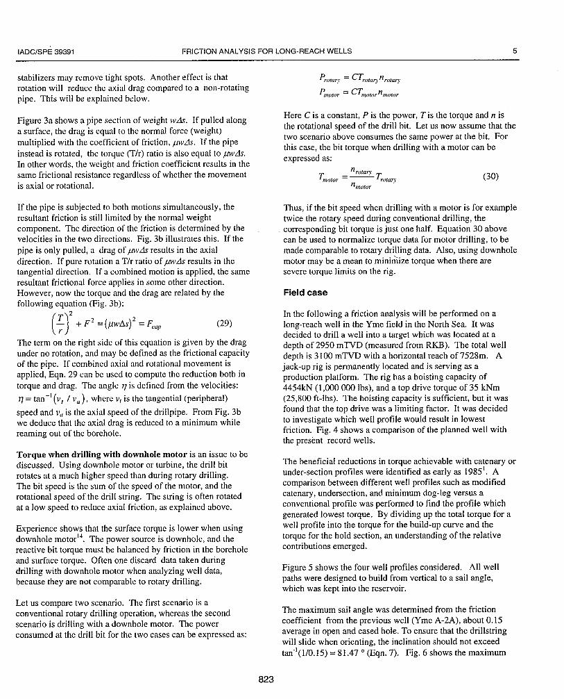
stabilizers may remove tight spots. Another effect is thatrotation will reduce the axial drag compared to a non-rotatingpipe. This will be explained below.
Figure 3a shows a pipe section of weight YVAS. If pulled alonga surface, the drag is equal to the normal force (weight)multiplied with the coefficient of friction, WVAS. If the pipe
instead is rotated, the torque (T/r) ratio is also equal to ,uwAs.In other words, the weight and friction coefficient results in thesame frictional resistance regardless of whether the movementis axial or rotational.
If the pipe is subjected to both motions simultaneously, theresultant friction is still limited by the normal weightcomponent. The direction of the friction is determined by thevelocities in the two directions. Fig. 3b illustrates this. If the
pipe is only pulled, a drag of IOVASresults in the axialdirection. If pure rotation a T/r ratio of ,uwAs results in thetangential direction. If a combined motion is applied, the sameresultant frictional force applies in some other direction.However, now the torque and the drag arc related by thefollowing equation (Fig. 3b):
()T2— + Fz = (#w’As)2 = FC,lPr
(29)
The term on the right side of this equation is given by the dragunder no rotation, and may be defined as the frictional capacityof the pipe. If combined axial and rotational movement isapplied, Eqn. 29 can be used to compute the reduction both in
torque and drag. The angle 71is (.lcfined from the velocities:
q= tan-’ (v, / v~), wher e v, is the tangential (peripheral)
speed and )1,,is the axial speed of the drillpipe. From Fig. 3bwe deduce that the axial drag is reduced to a minimum whilereaming out of the boreholc.
Torque when drilling with downhole motor is an issue to bediscussed. Using downhole motor or turbine, the drill bitrotates at a much higher speed than during rotary drilling.The bit speed is the sum of the speed of the motor, and therotational speed of the drill string. The string is often rotatedat a low speed to reduce axial friction, as explained above.
Experience shows that the surface torque is lower when usingdownhole motorl~. The power source is downhole, and thereactive bit torque must be balanced by friction in the boreholeand surface torque. Often one discard data taken duringdrilling with downhole motor when analyzing well data,because they are not comparable to rotary drilling.
Let us compare two scenario. The first scenario is aconventional rotary drilling operation, whereas the secondscenario is drilling with a downhole motor. The powerconsumed at the drill bit for the two cases can be expressed as:
Here C is a constant, P is the power, T is the torque and n isthe rotational speed of the drill bit. Let us now assume that thetwo scenario above consumes the same power at the bit. Forthis case, the bit torque when drilling with a motor can beexpressed as:
(30)
Thus, if the bit speed when drilling with a motor is for exampletwice the rotary speed during conventional drilling, thecorresponding bit torque is just one half. Equation 30 abovecan be used to normalize torque data for motor drilling, to bemade comparable to rotary drilling data. Also, using downholemotor may be a mean to minimize torque when there aresevere torque limits on the rig:
Field case
In the following a friction analysis will be performed on along-reach well in the Yme field in the North Sea. It wasdecided to drill a well into a target which was located at adepth of 2950 mTVD (measured from RKB). The total welldepth is 3100 mTVD with a horizontal reach of 7528m. Ajack-up rig is permanently located and is serving as aproduction platform. The rig has a hoisting capacity of4454kN ( 1,000000 Ibs), and a top drive torque of 35 kNm(25,800 ft-lbs). The hoisting capacity is sufficient, but it wasfound that the top drive was a limiting factor. It was decidedto investigate which well profile would result in lowestfriction. Fig. 4 shows a comparison of the planned well withthe present record welis.
The beneficial reductions in torque achievable with catenary orunder-section profiles were identified as early as 1985’. Acomparison between different well profiles such as modifiedcatenary, undersection, and minimum dog-leg versus aconventional profile was performed to find the profile whichgenerated lowest torque. By dividing up the total torque for awell profile into the torque for the build-up curve and thetorque for the hold section, an understanding of the relativecontributions emerged.
Figure 5 shows the four well profiles considered. All wellpaths were designed to build from vertical to a sail angle,which was kept into the reservoir.
me maximum sail angle was determined from the frictioncoefficient from the previous well (Yme A-2A), about 0.15average in open and cased hole. To ensure that the drillstringwill slide when orienting, the inclination should not exceed
tan-l( 1/0. 15) = 81.470 (Eqn. 7). Fig. 6 shows the maximum
823
6 B. S. AADNOY AND K. ANDERSEN IADCISPE 39391
sail angle as a function of well friction.
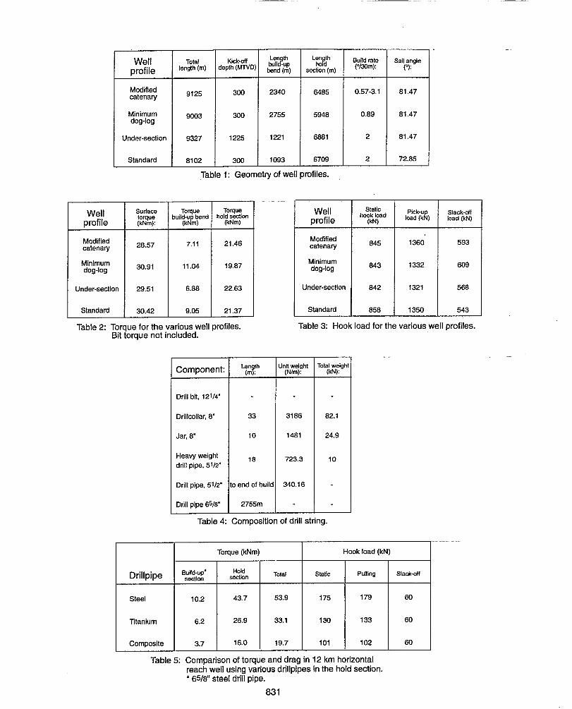
The geometries of the four well paths are defined in Table 1.Please observe that the measured lengths are different. Thelength and horizontal/vertical projections are calculated usingEqns.4, 12, 15 or Eqns. 23,24,27.
Table 2 shows the torque for the four well profiles. Themodified catenary profile gave lowest torque. Theundersection profile gave a little higher torque, but were betterthan the standard well profile. and the minimum dog-legprofile. Most of the torque is generated in the long sail section.
The hook loads for the four well profiles are shown in Table 3.The hook loads are similar, but the standard profile gives ahigher pick-up load than the other profiles. The maximumload is still less than half of the capacity of the drill pipe.Therefor tension is not the limiting factor.
From the evaluation of this particular well, the modifiedcatenary profile gave lowest torque. The minimum dog-legprofile can be preferred because it can be drilled with aconstant build rate.
To demonstrate the application of the analytical equations, anexample of determining the hook load during hoisting will beperformed. The minimum dog-leg trajectory is used.
The buoyancy factor is from Eqn. 5, with a mud density of1.68 s.g.: ~ = 1-1 .68/7 .85 = 0.786. From Table 4, the totalweight the bottom-hole assembly is: 117 kN.
The weight of the bottom-hole-assembly and the drillpipe inthe sail section is: 117 kN + 0.34016 kN/m (5948-6 1)m =2152 kN. The buoyed weight is: 0.786 x 2152= 1691 kN.During pulling of the string, the total pull-load is for thissection (Eqn. 1):
1691 kN(cos 81.47° + 0.15 sin 81.47°) = 501.6 kN.
The pulling load at the top of the sail section is the load at theentrance of the build-up section. The section builds fromvertical to 81.47 degrees, an angle of 8 1.47°7r/I 80° =1.422rad. 5 I/Z in. drillpipe is used from the start of the sailsection to surface. The pulling load at the top of the buildsection becomes (Eqn.9):
F2 = 501.6e015-’*4z2
+ 0.786x0.34016(kN / ))z)xI93 l(m)eO’15’’4z2sin 81.47° =
= 621+ 632= 1252kN
The tension at the top of the well is”the tension at the kick-offpoint plus the weight of the vertical pipe, or:
Fz = 1252 -t-0.786x0.34016kN I mx300m = 1332kN
This short example demonstrates the application of theequations derived in this paper. Similar calculations can beperformed for pipe lowering and for torque. One element ofparticular interest is the application of the equations to thedrilling mode. From above it is seen that the buoyed weight ofthe bottomhole assembly is. 0.786 x132.2 kN = 104.3 kN.From Eqn. 1 the axial component providing bit force is given
by: 104.3 kNcos8 1.47° = 15.47 kN. During sliding, there isvery little bit force to be applied because the well is designedto barely allow sliding. However, when rotation is initiated theaxial friction will reduce as shown in Eqn. 29, resulting in anincreased bit load.
The complete bottom-hole assembly will be in compression,but the remainder of the drill string will be in tension. If ahigher bit load is applied, the neutral point (transitioncompression/tension) will move the drill pipe up. In generalit is acceptable to keep the bottom hole assembly incompression. However, we try to place the drilling jar awayfrom the neutral point, that is, either in tension or incompression. Usually we design the bottom-hole assembly tojust provide the required bit load, keeping the weight at aminimum.
One advantage the modified catenary profile has compared tothe minimum dog-leg profile is the fact that the build-upfriction is generated over a shorter length(975m vs. 2758 m).Friction reduction subs may therefore be applied over a muchshorter length, resulting in less cost. A significant part of thefriction of the modified catenary is due to the build-up beforethe catenary starts. If a slant rig could be used, this frictioncould be reduced to a minimum. See discussion in AppendixB3.
Guidelines to obtain a low friction well profile
Based on the study the following general guidelines will beproposed to obtain a low friction well profile.
1. Keep as high inclination as possible on the sail section. Thisresults in a low tension at the end of the build-up section.
2. The weight of the bottom-hole assembly should be as low aspossible. Providing the required bit load is sufficient. Thedrill string should also have minimum weight.
3. If different pipe sizes are used, place the heaviest pipe in thevertical section.
4. Maintain a minimum dog-leg through the well. Also keepthe tortuosity at a minimum.
5. Use a modified catenary profile or a minimum dog-leg
824
lADC/SPE 39391 FRICTION ANALYSIS FOR LONG-REACH WELLS 7
profile if possible. For horizontal wells, the catenary is notrecommended as the low tension results in a high buildrate.lightweight composite drillpipes are used, tension reducescorrespondingly, reducing the need for a catenary profile.
If
6. The modified catenary often has a shorter build-up sectioncompared to the minimum dog-leg profile. This may reducethe cost of friction-reducing subs if used. Use torque reductionsubs where the side forces arc highest
7. Use low weight drill pipe, with small outer diameter tooljoints and hard banding, with self-lubricating matrix. Thisreduces weight, increases buoyancy and results in less wellfriction.
8. Select a sufficient high flow rate to ensure adequate holecleaning’d. Keep annular cuttings concentration 10W’6.
Johansik, Friesen and Dawson’8 shows the field analysis oftorque and drag.
Example of ultra-long reach well design
The record long-reach wells today is approaching 8 kmhorizontal reach. However it is fully feasible to extend thistowards and even beyond 12 km by a well planned design anda operational follow-up. Below arc a few points of concern.
The well profile should be as simple as possible consisting of avertical section, a build section and a sail angle towards thetarget. Avoid drop-off into the reservoir if possible tominimize friction.
The sail arlgle should in general be as high as possible, toreduce axial tension and hence friction in the curved holesections. Usually the reservoir depth is such that the target iswithin reach only if a very high sail angle is used. Themaximum sail angle is given by the friction coeflicie~zt.Therefore, another requirement is low friction. This can beobtained by using oil muds or friction reducers.
The wells will often be designed with a constant sail angle intothe reservoir. The transition from vertical to this sail anglemay follow a modified catenary curve or a minimum dog-legprofile, as these will provide minimum friction.
To limit the load on the drillpipe, a high blloyarzcy can bebeneficial. The disadvantage of a dense fluid is thecompromise between buoyancy and friction. Usually moreparticles in the mud will increase the frictions.
In long wells hydraulic friction may limit the flow rate, thusleading to poor hole cleaning. Increased pipe size will reducethis problem. Since increased pipe size leads to increased pipeweight, drill pipes of alternative materials may be required.
Today drill pipes are available both in aluminum, titanium andcomposites.
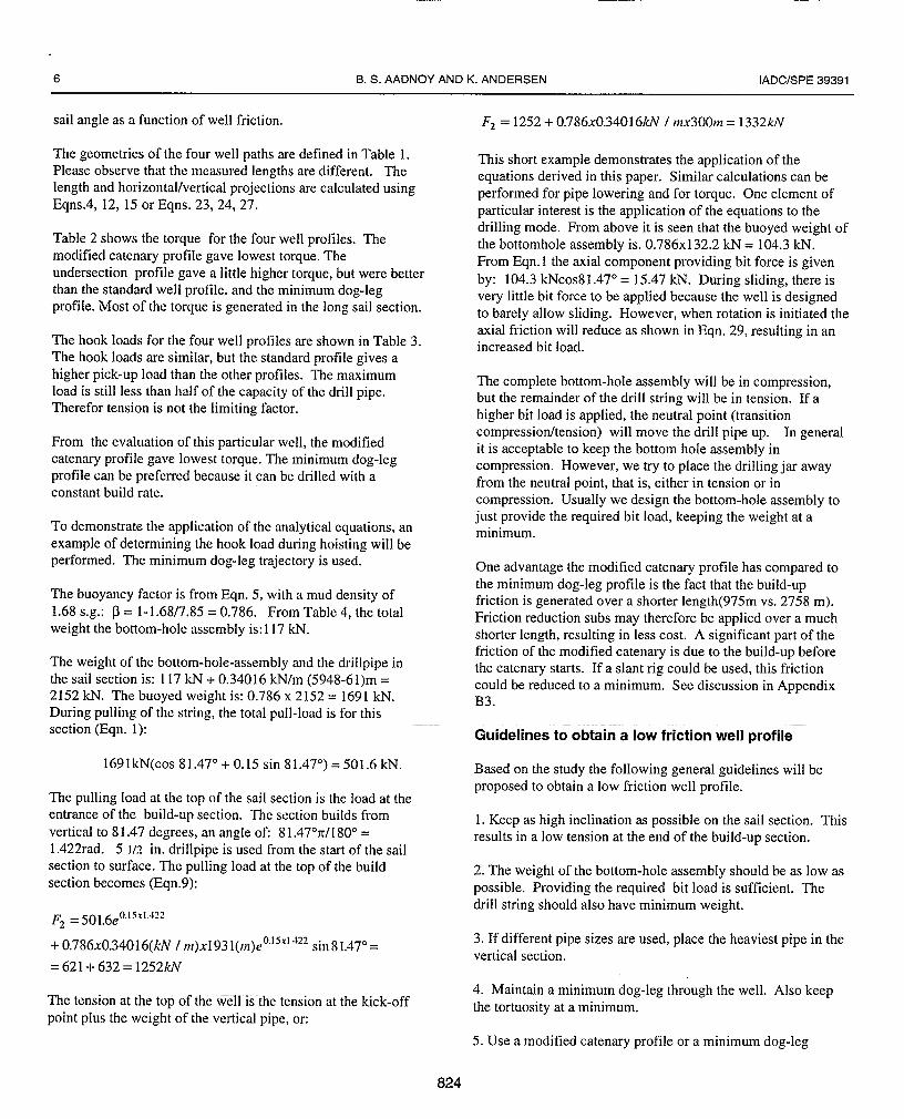
In the following an example of extending the Yme well from areach of 7528 m to 12 km will be shown. Figure 6 shows theresulting well path. Maintaining the same sail angle, this wellwill reach the target at a depth of 3767 mTVD (from RKB).The build-up section is the minimum dog-leg profile.
A analysis of the hydraulics and hole cleaning problems ofsuch a long well resulted in the conclusion that the drill stringshould have an outer diameter of at least 5.5 in. The analysisis therefore assuming a 6 5/8 in drillpipe in the upper 2755 m,
‘and 5.5 in drill pipe down to the bottom-hole-assembly.
Due to the fact that most of the drill string is located in the sailsection, the hook load is reasonably low. Table 4 shows theresults. The hook load is not a limiting factor during drillingof the well.
Table 5 shows the torque for the case of using 5.5 in. drillpipethroughout. The total predicted torque is 53.9 kNm.Although a few drilling rigs can handle torque of thismagnitude, it is too high for Yme, which has an upper torquelimit of 35 kNm.
It was decided to try with a light drillpipe. Most of the torqueis generated from tension from the sail section which isconverted into torque in the build section. The sail section wastherefore first modeled with a drill pipe made of titanium. Asseen in Table 5, the torque drops to 33.1 kNm. Sincecomposite drill pipes now are available]G (8.72 lb/ft), the sailsection was also modeled with this as well. The cumulativetorque was now down to 19.7 kNm. Bit torque must be added.
From this study it is concluded that it is fully possible to drillextended reach well to 12 km. Actually, by using lighter drillpipes as shown, it should be possible to drill severalkilometers beyond that.
Other elements of long-reach wells
This paper has primarily focused on well friction, whichprovides strong limitations as the wells become long.However, a number of other elements must be handled as wellin order to drill a successful well’”. In the following, the mostimportant of these are discussed.
Casing wear may become excessive in long wells. This is adirect result of well friction. Therefore, all measuresaddressed above to minimize friction leads to reduced casingwear.
Borehole stabili~ problems may lead to drilling problems.
825
8 B. S. AAUNUY AND K. ANDtH5kN l~u~/arK dY6Y I
Examples are circulation losses, and borehole collapse whichmayresult in stuck pipe. Thedrilling fluid should becomposed to handle this. Inparticular, the mudweight playsakey role. Aadn@y15discusses optimal mudweight selection.
Holecleaning provides another constraint. Cuttingsaccumulation in the annulus may lead to higher bottom-hole-pressure, which sometimes leads tocirculation losses. Anotherconsequence ofcuttings accumulation may be stuck pipe. Theoperational procedures must ensure good hole cleaning*5.Also, the flow rate must be adequate to transport cuttings tosurface. Aadn@y*5propose optimization criteria for flow rateand bit nozzle selection.
Conclusions
In this paper friction models for a number of different wellgeometry’s are derived. Explicit equations are derived tomodel both the rotary torque and the drag forces associatedwith hoisting or lowering of the drill string. Equations tocompute well friction for a fully 3-dimensional well path isalso given. Equations for combined motion and for drillingwith a motor are also given. These equations can be appliedto any type of well using e.g. a spreadsheet.
The models are applied to a long-reach well offshore Norway.It is shown that by proper well path design, the torque and dragcan be reduced to a minimum.
The models are furthermore used to study ultra-long-reachwells. It is fully possible to drill beyond 12 horizontal reach,provided that light-weight drill pipes are used.
The most important factor in drilling ultra-long wells is to uselow weight drillpipe. This reduces tension and increasesbuoyancy, leading to less friction and less casing wear. Otherkey elements are low friction coefficient, and high buoyancyby using adequate mud density.
Acknowledgments
The authors wish to thank Tor Iver Sakkestad, Statoil Bergenand Odd Bj@rnar Ness, Statoil R&D for support in developingthe models. Also, we wish to acknowledge Statoil as. forpermission to publish the paper.
Nomenclature
X,y = coordinates in the horizontal planez = vertical coordinate
S, A.s= measured length along hole section
~, ,4y, & = projected distancesw = unit weight of drillpipe (kg/m)F= force along drillstring (kN)F1 = force at bottom of section
Fz = force at top of sectionT= torque along drillstring (kNm)P = power(kW)n = rotary speed (rPm)C = conversion constant
a = inclination of string from vertical (rad)$= azimuth of the section (rad)
AF = additional force applied to catenaryWOB = weight-on-bitBHA = bottom-hole-assemblyR = radius of bend (m)r = radius of tool joint (m)
TVD = true vertical depth (m)RKB = drill floor referenceDL = dog-leg; angular change in well pathDLS = dog-leg severity; rate of dog-leg
=30 (m) x 57.3 (O/rad)/R(m)
cr = sign constant for various directionsand geometry’s
,.aP= frictional capacity of the drill stringFq = tangential speed/axial speed of the drillpipe
References
1. Sheppard, M. C., Wick, C. and Burgess, T. Designing wellpaths to reduce drag and torque. SPE Drilling Engineering,Dec., 1987, pp. 344-350.
2. Banks, S.M,, Hogg, T.W. and Thorogood, J,L. Increasingextended-reach capabilities through wellbore profileoptimization. Paper IADC/SPE 23850 presented at the 1992IADC/SPE Drilling Conference, New Orleans, Feb. 18-21.
3. McClendon, R.T. and Anders, E.O. Directional drillingusing the catenary method. Paper SPE/IADC 13478 presentedat the 1985 SPWIADC Drilling Conference, New Orleans, La.,March 6-8.
4.Eek-Olsen, J., Sletten, H., Reynolds, J.T. and Samuell, J.G.North Sea advances in extended reach drilling. PaperSPEIIADC 25750 presented at the 1993 SPE/IADC DrillingConference, Amsterdam, Feb. 23-25.
5. Eek-Olsen, J., Drevdal, K.E., Samuell, J. and Reynolds, J.Design directional drilling to increase total recovery andproduction rates. Paper SPE/IADC 27461 presented at the1994 SPE/IADC Drilling Conference, Dallas, Texas, Feb. 15-18.
6. Alfsen, T.E., Heggen, S., Blikra, H. and Tj@tta, H. Pushingthe limits for extended reach drilling: New world record fromplatform Statfjord C, well C2. Paper SPE 26350 presented atthe 68th Ann. Tech. Conf and Exhibition of the SPE, Houston,Texas, Oct. 3-6.
826
iADC/SPE 39391 FRICTION ANALYSIS FOR LONG-REACH WELLS 9
7. Justad, T., Jacobsen, B., Blikra, H., Gaskin, G., Clarke, C.and Ritchie, A., 1995. Extending barriers to develop amarginal satellite field from an existing platform. PaperSPE/IADC 28294 presented at the 69’h Ann. Tech. Conf. of theSPE, New Orleans, Sept. 25-28, 1994.
8. Blikra, H., Drevdal, K.E. and Aarrestad, T.V. Extendedreach, horizontal and complex design wells: challenges,achievements and cost-benefits. Presented at the 14t}’WorldPetroleum Congress, Stavanger May 29-June 1, 1994.Proceedings VO1.2, pp. 191-201.
9. Aarrestad, T.V. and Blikra, H. Torque and drag - twofactors in extended-reach drilling. Journal of PetroleumTechnology, Sept., 1994, pp. 800-803.
10. Payne, M. L., Cocking, D.A. and Hatch, A. J. Criticaltechnologies for success in extended reach drilling. Paper SPE28293 presented at the SPE 69’}’Ann. Tech. Con$ andExhibition, New Orleans, LA, Sept. 25-28, 1994.
11. Benesch, J.M., Camacho, G., Matsuzawa, S. and Dawson,C.R. Planning a record extended-reach well in Japan.Petroleum Engineer International, April, 1996, pp. 59-67.
12. Gou, R., Lee, R.L. and Miska, S.. Constant curvatureequations improve design of 3-D well trajectory. Oil and GasJournal, Apr. 19, 1993, pp. 38-47.
13. Wiggins, M. L., Choe, J. and Juvkarn-Void, H.C. Singleequation simplifies horizontal, directional drilling plans. Oiland Gas Joltrnal, Nov. 2, 1992, pp. 74-77.
14. Guild, G. J., Hill, T. H. and Summers, M. A. Designing anddrilling extended reach wells. Petroleum EngineerInternational, Jan. 1995, pp. 35-41.
15. Aadn@y, B.S. Modern Well Design. First edition.Balkema, Rotterdam, Netherlands 1996).ISBN905410 6336
16. Bourgoyne, A. T, Millhcim, K. K., Chenevert, M. E. andYoung, F. S. Applied drilling engineering. SPE TextbookSeries, Vol. 2., first ed. 1986. ISBN 1-55563-001-4.
17. Hareland, G., Lyons, W. C., Baldwin, D. D., Briggs, G. andBratIi, R.K. Extended reach composite materials drill pipe.Paper SPEIIADC 37646 presented at the 1997 SPE/IADCDrilling Conference, Amsterdam, March 4-6.
18. Johansik, C.A., Friesen, D.B. and Dawson, R. Torque anddrag in directional wells - prediction and measurements. PaperIADC/SPE 11380 presented at the 1983 IADC/SPE DriIIingConference, New Orleans, Louisiana, Feb. 20-23.
Appendix Al: Drag and torque in drop-off bends
We will in the following derive equations to calculate dragforces when a drillstring is pulled or lowered through a bend.Figure Al. 1 shows the forces acting when a pipe is pulledthrough a drop-off section. Before doing the actual analysis, afew parameters need to be defined. Due to the bend, a normalforce N results between the driIlstring and the hole. Whilepulling the string, a frictional force Q resist the motion. Theweight of the string is the unit weight w multiplied with the
length of the differential element, wRda Choosing a X,Zreference system the weight can be decomposed into thefollowing components:
P = wRdacosa and O = wRda.rina
Performing a force balance in the x and z directions results inthe following equations:
~Fx = O: (F+ dF)cosd& - Fcosdd2- Q - P = O
ZFZ = O: N -0 -(F+ dF)sind& - Fsindd = O
The resisting friction force Q is equal to the coefficient offriction v multiplied with the resulting normal force, that is: Q= pN. Furthermore, for small arguments, cosda/2 = 1, and
sindu/2 = dci12. The force balance above can be shown tobecome:
dF= Q i- P = Q i- wRdacosa (All)
N = Fda+ O = Fda i- wRdasina (A1.2)
Combining the equations above, the equation for the tension inthe drillstring becomes:
dF= {FF +wR(pina + cosa)) da (A1.3)
Integrating equation A 1.3, the final solution for theadditional force through the bend is given by:
Fz = F’e#t%-alj
[
WR (1–p2)(sina2–e )~(az‘~1 sin al)
}
(Al .4)+—
1+p2 – 2p(cos a2 – e,u(a2-cY,) Cos ~, ~
Here F1 refer to the tension at the bottom and F2 to the tensionat the top of the bend.
The above equation is valid for the case of pulling the---- drillstring upwards. If the drillstring is lowered into the well,
the forces F and F+dF interchange places in Fig. Al. 1, and thefriction force Q change direction. The force balance nowbecome:
dF= Q - P = Q - wrdacosa
827
io B. S. AADNOY AND K. ANDERSEN IADCISPE 39391
N= Fda+O=Fda +wRdasina, resulting in thefollowing differential equation:
dF= {pF+i~tR(/6ina-cr~sa}da, which gives thesolution:
){
-~(az-ffl +)ltR sin~~ –e}
-P(az-rrl) sina, (A1.5)Fz = Fle
Note thatthe forccshave forthis case been redefined. Fzisalways referring to the force in the top of the string.
The frictional torque isequal tothe normal force multipliedwith the pipe radius, integrated over the length of the bend,
ds=rda. Thetension inthepipe forastatic pipe is:
F = F, – wR(sin a – sin al ) (A1.6)
Thegeneral expression forthetorque becomes, using Eqn.A.1.3, and 1.6:
T= JprN (A1.7)
Integrating the equation above, the resulting torque for a drop-off bend becomes:
{T=pr F1–wRsincil
}(~2-~1)-~~”R(cos~2-cos~l)(A1.8)
Appendix A2: Drag and torque in build-up bend
Figure A2. 1 shows the forces in a build-up section. The basicdefinitions are the same as for the previous case. A forcebalance now results in:
ZF.V = O: (F -t dF)cosd& - Fcosdd2- Q - P = O
ZFy = O: N + O -(F+ dF)sind& - Fsindd2 = O
Repeating the previous analysis, the force balance abovebecomes:
dF= Q + P = Q -!-wrdacosct (A2.1)
N = Fda -0 = Fda - wRdasina (A2.2)
Repeating the previous analysis, it can be shown that the pullforce now is defined by:
dF= (pF -wR(pina - cosa)) da (A2.3)
F2=F1e -~(ff~-ffl) _{
wIR sin az – e –p(az-a2 )}
sin al (A2.4)
Finally, for the case of lowering the pipe through the build-upbend results in: dF = Q - P
dF= {,F-wR(pinci + cosaj da (A2.5)
which solved again defining F2as the top force, becomes:
F,= F1e~(a2-al)
[
( )[l–pz sin ffz – ep(a2-a, ) .
WR sln al1
1
(A2.6)_—
l+p2[
–2p cosaz –e )fl(~2-al Cosa,)
Repeating the process for build-up bends as given in Eqn.A 1.7, the torque becomes:
T=
~r{(F1 +wRsinal)(~2 -~l)}+2~wRr(cos~2 -coSal)
(A2.7)
Appendix A3: Drag and torque in side-bends
In a side bend another complexity arise, which can bedescribed as follows.
Figure A3. 1 shows the situation. One extreme is that the drillpipe is weightless. For this case pure tension applies, and thepipe will assume a position in the middle of the borehole.Based on previous derivations, we can define the end force ofthe bend due to tension as:
F21 = F1ep(&–4) (A3.1)
The normal force on the borehole wall is the tension multipliedby the angle, or:
dN, = Fd@ (A3.2)
The other extreme would be to assume the the pipe weight isthe dominating factor, resulting in the pipe lying on the bottomof the hole. The normal force is then:
dN~ = wRd@ (A3.3)
In reality, neither of the two extremes exist. The drillpipe mayassume a position at the bottom of the hole when entering thebend, and move towards ~ = 90° at the exit of the bend. Wewill assume that the resultant normal force is the vector sum ofEqns. A3.2 and A3.3.
dN = ~dN; +dN; (A3.4)
828
lADC/SPE 39391 FRICTION ANALYSIS FOR LONG-REACH WELLS 11
The friction in the boreholc is equal to the resultant normalforce, multiplied with the coefficient of friction, or:
EFr=O+Fcosa –FOsincrl =0
ZFZ =O+Fsina– ws– F1cosal =0
or combined:
dF=p~F2 +(wR)2d@ (A3.5)
Integrating Eqn. A3.5, the general solution is:
,og{F+-}=PfP+c (A3.6)
The constant of integration, c, is determined by inserting the
initial condition (Fl, $l). Applying the other end condition, thetension at the upper end of the side bend is given by:
(A3.7)A similar expression results for lowering of the pipe. Thedifference is that the exponents changes sign.
The pipe position on the borehole wall can be determined bydefining a tangential force balance as seen from Fig. A3. 1:
Inserting zero friction into Eqn. A3.7, one observe that F2 = Fl.For pure rotation , the torque is generated by a constant normalforce (weight) as defined in Eqn. A3.4. The total torquebecomes:
‘=~’e(@2 -@*)(A3.9)
Appendix B1: The modified catenary profile
In the catenary profile the rate of inclination build increasescontinuously to mimic the shape of a hanging cable.Theoretically, a catenary produces very low torque and drag asa result of very low contact forces between the string and thewall of the hole.
The classical catenary profile is limited as it requires ahorizontal end condition at bottom. This is illustrated in Fig.B 1.1. Here we will derive a more general solution witharbitrary inclinations at the bottom and at the top. Fig.B 1.2illustrates the end section assuming this. We have chosen to
introduce the well inclination al and tension force F, to definethe end condition at the bottom.
The force balance is:
F = F,* + (WS)2 + 2wsF, COSa,
The slope is given by:
dz ws+ F, COSaltarif f=-=
dx F, sin a,
(B1.1)
(BI.2)
The length of the string is still given by:
/7
2
ds2=dx2+dz2+ s(x)=] 1+ ~ (BI.3)
oCombining Eqns, B 1.2 and B 1.3 results in the followingdifferential equation:
By introducing the hyperbolic trigonometric function dtidx =sinhu, and differentiating, Eqn. B 1.2 can be shown to become:
du W—=
dx F, sin al
which integrated becomes:w
u = F, sin alX+c,
To determine the constant of integration, at the lower point ofthe string, x=O and z=O. Furthermore at this point the slope or
the derivative is no longer zero, but equal to sinh(fl-al).Inserting these conditions into the equation above results inC1=sinhl(cotal). The solution can now be written:
{
& = Sinhu = Sinh Wx
dx+sinh-l (cot al)
F, sin a, }
which when integrated results in:
F, sin al
{
w~.~z= cosh
F1 sin al }+sinh-l (cot al + C2
w
But z = Oat x = O. This determines the constant Cz. The finalexpression for the free-hanging string now becomes:
Fl sin alz= x
w
[{
Wxcosh
Fl sin al+ sinh ‘l(cota,)}-cosh{sinh(cotal)}]
(B 1.4)
829
12 B. S. AADNOY AND K. ANDERSEN IADCISPE 39391
Equation B 1.4 gives the shape of the curve. The total lengthmeasured along the string tnust be determined next. FromEqn. B 1.2, the total length of the string becomes:
F1
[{
}t:Ys =; sin al sinh
F] sin al+ sinh -I(c~t~,)}-cos~,]
(B 1.5By inserting Eqn. B 1.5 into B 1.1, the total tension at any pointin the string can be determined.
The rate of change at any point along the string is determinedby differentiating Eqn. B 1.2 with respect tos. This buildratecan be shown to vary along the string as follows:
da tLIF1sin ffl WF1sin ffl
x= F12+ (WS)2 + 2wsFl COSal – F2(B1.6)
Appendix B2: Drag and torque in modified catenaryprofiles.
We are concerned about the friction in the wellbore. This isgoverned by the normal force between the drillstring and thehole. Using the equations above, an ideal well profile resultswith zero normal force. The objective is to use this conditionduring drilling. However, when tripping out, an additionalforce must be applied. If we assume that the catenary designforces applies, the well will have an ideal catenary profile andthere is no contact between the hole and the drillstring duringdrilling (ideally). Next assume that the drillstring will betripped out of the well. By pulling in the string, it contacts theborehole wall resulting in drag friction. We assume that theadditional force at the bottom of the drillstring is AF. If thedrill string remains static, this additional force will be reflectedfrom the bottom to the top of the catenary section.
The normal force caused by this additional force can becalculated at any point using the equation:
()~_daAF
ds(B2.1)
Assuming a coefficient of friction, p, in the borehole, the dragforce seen at top of the catenary is given by:
(B2.2)
Inserting Eqn. and B 1.6 into B2.2, and integrating, thefollowing equation results:
AFCut= pAF tan-’{’VS;::;U’}
(B2.3)
The total load at the top of the catenary during tripping is nowgiven by:
830
F2 i- AFCal (B2.4)
If the pipe is lowered, the tension in the top is reduced with-AF, and the tension at the bottom of the catenary is:
Ft – AFCa, (B2.5)
The torque is given by:
JATCO,= ~ prANds = prAF tan” {Ws;::(B2.6)
Appendix B3: Entrance condition to the catenarycurve
It is obvious from Flg.B 1.2 that the modified catenary solutionrequires a non-vertical entrance at the top. This problem has inthe past been handled by defining a short constant-curvaturebuild section from the vertical well to the entrance of thecatenary. In land wells, it is possible to start the well at a givenangle using a slant rig.
We will define a simple function to make a continuous smoothtransition from vertical to the start of the catenary.
Figure B 1.2 shows that the catenary starts at an angle crzfromvertical. We will choose to add a short constant curvaturebuild-up section on top to go to vertical. To make thetransition smooth, we will design the intersection between thetwo functions to have the same curvature.
Eqn. B 1.6 defines the curvature for the modified catenary. Atthe top of the catenary, the inclination and curvature is:
dz ws + FOCOSaltanaz =—=
dx FOsin al(B3.1)
da2 WFOsin al—.ds – F02+ (WS)2 + 2WSF0 cOSal
(B3.2)
A build-up section on the top of the catenary is defined by:
As = Rcr2 (B3.3)
and its derivative:dcz~ds = I/R (B3.4)
Equating Eqns. C3.2 and C3.4, the radius of the build-upsection becomes:
~ = FO+ (WS)2 + 2WSF0 COSal
WFOsin al(B3.5)
Here the subscripts 1 refers to the bottom of the modifiedcatenary, and 2 to the top of the modified catenary. Fig. B3. 1shows the transition section.
Well Total Kisk-offLe&~h
;tidg;’pBuild rate Sail angle
profile length(m) depth(MTVD) ~nd (~) sestbn (m) (’=/3omfi (“):
t
Modifiedcatenary 9125 300 2340 6485 0.57-3.1 81.47
Minimumdog-log
8003 300 2755 5948 0.89 81.47
Under-section 9327 1225 1221 8861 2 81.47
Standard 8102 300 1093 8709 2 72.85
,Tablel: Geometry ofwell profiles.
Wellprofile
Modifiedcatenary
Minimumdog-log
Under-section
Standard
Surface
;?$:
28.57
30.91
29.51
30,42
buil;’p;”
7.11
11.04
6.88
9.05
Toquehold section
(kNm)
21.46
19.87
22.63
21.37
Wellprofile
Modifiedcatenary
Minimumdog-log
Under-section
Standard
Statichmk load
(kN)
845
843
842
858
pick-upload (kN)
1360
1332
1321
1350
—
Slack-offload (kN)
593
609
568
543
Table2: Torque forthevarious well profiles. Table 3: Hook load for the various well profiles.Bit torque not included.
Component:
Drill bit, 121/4”
Drillcoliar, 8“
Jar, 8“
Heavy weight
drill pipe, 51/2”
Drill pipe, 51/2”
Drill pipe 65/8”
Length(m):
33
10
18
I end of build
2755m
)n~ww;~
3186
1481
723.3
340.16
rota~~:ghl
82.1
24.9
10
Table 4: Composition of drill string.
Torque (kNm) Hook load (kN)
Drillpipe B;~d~~* Holdeedmn Total Static Pulling Slack-oft
Steel 10.2 43.7 53.9 175 179 60
Titanium 6.2 26.9 33.1 130 133 60
Composite I 3.7 / 16.0 I 19.7 I 101 \ 102 I 60
Table 5: Comparison of torque and drag in 12 km horizontalreach well using various drillpipes in the hold section.* 65/8” steel drill pipe.
831

Figure 1: Forces and geometry in straight hole sections.
Az
‘= :{-:;’,lI I
x x
a) Forceson Inolinedobject b) Geometry and forces for straight inclined hole
.—— ——
x
Axa) DrW.off eeetlon
Y
Ax
c) Riihl sidebend
Ax
K
F2
As
b) Build-up aesfien
Y
IAz
,—.
Az
IK
It
I
I
I
I
As I
\;
e) The mcdifled ~tenary profile
F2
t Ax
{~
az
Az el
a F,
‘1iAx
d) Left side band0 Entranse 10 the modfti ca!enary
Figure 2: Forces and geometries of various curved hole
F=PWAS T/r.pwAs
Torque/radius I
PWAS
T/r
a) Drag and torque for a pipe.
b) Combined friction from rotation and axial movement.
Figure 3: Combined friction.
832

Horizmtal dapanure, m
o Im 2m m 4W0 5m 6~ 7m
I I I I
w
I
I 1 1 , ---- . . .z-t ,00 0 .L . . . .
# \
I,w,,~r!”
J I
-\\o
t
YEe$ 0 >,0 Ula \\
-. 0 I~ 4000.
\00 \
! \
7000
Figure 4: Present extended reach wells.
o — Statiard, build rate 2“/SOm
m ._ Mnimum dog-%, 0.09 “13~. . . . Mdifiti catenary. CMII build 0.57”m,
w.975m to sta~01 catenav_ - under.~~ti~ , 2“l%m
1225-
- \*”.\.
2000- \“’.\- ● .’.- ●
___
3ow- .-
3ritical sailsngle, degrees
90-
85-
81.47 —————
80- I
I
I
I75-
I
I
I
70 I [ Io 0.10
0.15 0120O.w 0.40 COeffj~ie”tOf
friction, u
Figure 5: Profiles considered for the Yme well.
Figure 6: Critical sail angle versous friction coefficient.
o
Im 65/8” atsel drillpipe
2000-
3m -
40001
nTVO, , , ! I , I I J r 1 ,
0 1Oco 2W0 3m 4m Sm m 7m m eooo Im Ilow Izm
m horizontal reach —-.Figure 7: Extending the Yme well to a horizontal reach of 12 km.
833
d.
F+dF
‘\\
\
x
>\ / \
\vz“ wrda
Figure A2.1: Forces acting on a drillpipe elementin a build-up section.
Figure A3. I: Drill pipe position in the borehole for a side bend.
‘ F+dF/’fl
—Figure Al.1: Forces acting on a drillpipe element
pulled in a drop-off section.
F2
Ax
I
I/ x
U2>
I /
I /
I/
,
I
I
I
I ,’/
/.—— —
//
Figure B3.1: Transition from vertical to modified catenati.
WFZ,.;%$: .~~L*- JJa) b) z
Figure BI.1: Shape of a free-hanging rope. xF1 al
Figure B1 .2: Modified catenary string.