NASA TECHNICAL NOTEA/93-NASA TN D-7266

I*-.Q

c

THREE-DIMENSIONAL ELASTIC STRESS

AND DISPLACEMENT ANALYSIS

OF FINITE CIRCULAR GEOMETRY

SOLIDS CONTAINING CRACKS

by John P, Gyekenyesi, Alexander Mendelson,

and Jon Kring

Lewis Research Center

Cleveland, Ohio 44135

NATIONAL AERONAUTICS AND SPACE ADMINISTRATION • WASHINGTON, D. C. • MAY 1973

https://ntrs.nasa.gov/search.jsp?R=19730016164 2018-07-19T04:58:30+00:00Z

1. Report No.

NASA TN D-72662. Government Accession No. 3. Recipient's Catalog No.

4. Title and Subtitle THREE-DIMENSIONAL ELASTIC STRESS AND

DISPLACEMENT ANALYSIS OF FINITE CIRCULAR

GEOMETRY SOLIDS CONTAINING CRACKS

5. Report DateMay 1973

6. Performing Organization Code

7. Author(s)

John P. Gyekenyesi, Alexander Mendelson, and Jon Kring8. Performing Organization Report No.

E-7258

9. Performing Organization Name and Address

Lewis Research CenterNational Aeronautics and Space AdministrationCleveland, Ohio 44135

10. Work Unit No.

501-2111. Contract or Grant No.

12. Sponsoring Agency Name and Address

National Aeronautics and Space AdministrationWashington, D. C. 20546

13. Type of Report and Period Covered

Technical Note

14. Sponsoring Agency Code

15. Supplementary Notes

16. Abstract

A seminumerical method is presented for solving a set of coupled partial differential equationssubject to mixed and coupled boundary conditions. The use of this method is illustrated byobtaining solutions for two circular geometry and mixed boundary value problems in three-dimensional elasticity. Stress and displacement distributions are calculated in an axisymmetric,circular bar of finite dimensions containing a penny-shaped crack. Approximate results for anannular plate containing internal surface cracks are also presented.

17. Key Words (Suggested by Author(s))

Three-dimensional; Elasticity; Stress; Dis-placement;'-..Penny-shaped crack^ Stress inten-sity factor; Circular-geometry

18. Distribution Statement

Unclassified - unlimited

19. Security Classif. (of this report)

Unclassified20. Security Classif. (of this page)

..";. Unclassified21. No. of Pages

46.

22. Price*

$3.00

*For sale by the National Technical Information Service, Springfield, Virginia 22151

CONTENTS

PageSUMMARY 1

INTRODUCTION 1

SYMBOLS 3.

REDUCTION OF THE NAVIER-CAUCHY EQUATIONS TO

SYSTEMS OF ORDINARY DIFFERENTIAL EQUATIONS 4'

SOLUTION OF THE SYSTEMS OF ORDINARY DIFFERENTIAL EQUATIONS ... 9

NUMERICAL RESULTS 12

Solid Cylindrical Bar with a Penny-Shaped Crack 12Annular Plate with Internal Surface Cracks 18

STRESS INTENSITY FACTOR 26

APPENDIXES

A - SOLUTION OF SIMULTANEOUS DIFFERENTIAL EQUATIONS

WITH VARIABLE COEFFICIENTS 29B - SOLUTION OF SIMULTANEOUS DIFFERENTIAL EQUATIONS

WITH CONSTANT COEFFICIENTS 34C - DEVELOPMENT OF THE INITIAL VALUE VECTORS 38

REFERENCES 43

ill

Page Intentionally Left Blank

THREE-DIMENSIONAL ELASTIC STRESS AND DISPLACEMENT ANALYSIS

OF FINITE CIRCULAR GEOMETRY SOLIDS CONTAINING CRACKS

by John P. Gyekenyesi, Alexander Mendelson, and Jon Kring

Lewis Research Center

SUMMARY

Displacement and stress distributions are calculated in finite circular bars, eachcontaining a penny-shaped crack and loaded normal to the crack surface. Similar re-sults are presented for an annular plate containing internal, traction-free surfacecracks. The Navier-Cauchy equations of elastic equilibrium are reduced to three setsof coupled, simultaneous, ordinary differential equations whose solutions are obtainedalong sets of lines in a discretized region. Since decoupling of these equations and theirboundary conditions is not possible, a successive approximation procedure is applied toobtain their analytical solution. These analytical solutions are compared with known so-lutions, and the results of the circular bar are used to examine the rate of convergenceand the accuracy of this method. The results obtained show that the method of linespresents a systematic approach to the solution of some three-dimensional elasticityproblems with arbitrary boundary conditions. The advantage of this method over othernumerical solutions is that good results are obtained even from the use of a relativelycoarse grid.

INTRODUCTION

The object of a problem in elasticity is usually to calculate the displacement andstress distributions in an elastic body which is subject to given body forces or surfaceconditions. These distributions are the solutions of the applicable field equations whichmathematically model the behavior of engineering materials. The solution of this gen-eral system of equations is, however, usually too difficult to evaluate. At present, fewanalytical solutions of three-dimensional problems exist (ref. 1), and even these solu-tions frequently require symmetry conditions to simplify the governing equations. Re- 'cently, with the introduction of large digital computers, the use of a number of approx-

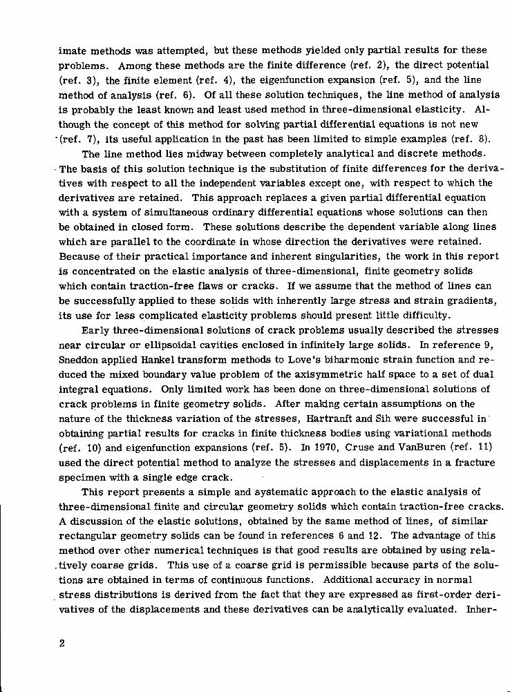
imate methods was attempted, but these methods yielded only partial results for theseproblems. Among these methods are the finite difference (ref. 2), the direct potential(ref. 3), the finite element (ref. 4), the eigenfunction expansion (ref. 5), and the linemethod of analysis (ref. 6). Of all these solution techniques, the line method of analysisis probably the least known and least used method in three-dimensional elasticity. Al-though the concept of this method for solving partial differential equations is not new

'(ref. 7), its useful application in the past has been limited to simple examples (ref. 8).The line method lies midway between completely analytical and discrete methods.

• The basis of this solution technique is the substitution of finite differences for the deriva-tives with respect to all the independent variables except one, with respect to which thederivatives are retained. This approach replaces a given partial differential equationwith a system of simultaneous ordinary differential equations whose solutions can thenbe obtained in closed form. These solutions describe the dependent variable along lineswhich are parallel to the coordinate in whose direction the derivatives were retained.Because of their practical importance and inherent singularities, the work in this reportis concentrated on the elastic analysis of three-dimensional, finite geometry solidswhich contain traction-free flaws or cracks. If we assume that the method of lines canbe successfully applied to these solids with inherently large stress and strain gradients,its use for less complicated elasticity problems should present little difficulty.

Early three-dimensional solutions of crack problems usually described the stressesnear circular or ellipsoidal cavities enclosed in infinitely large solids. In reference 9,Sneddon applied Hankel transform methods to Love's biharmonic strain function and re-duced the mixed boundary value problem of the axisymmetric half space to a set of dualintegral equations. Only limited work has been done on three-dimensional solutions ofcrack problems in finite geometry solids. After making certain assumptions on thenature of the thickness variation of the stresses, Hartranft and Sih were successful inobtaining partial results for cracks in finite thickness bodies using variational methods(ref. 10) and eigenfunction expansions (ref. 5). In 1970, Cruse and VanBuren (ref. 11)used the direct potential method to analyze the stresses and displacements in a fracturespecimen with a single edge crack.

This report presents a simple and systematic approach to the elastic analysis ofthree-dimensional finite and circular geometry solids which contain traction-free cracks.A discussion of the elastic solutions, obtained by the same method of lines, of similarrectangular geometry solids can be found in references 6 and 12. The advantage of thismethod over other numerical techniques is that good results are obtained by using rela-

.tively coarse grids. This use of a coarse grid is permissible because parts of the solu-tions are obtained in terms of continuous functions. Additional accuracy in normalstress distributions is derived from the fact that they are expressed as first-order deri-vatives of the displacements and these derivatives can be analytically evaluated. Inner-

herently inaccurate numerical differentiation is required only for the evaluation of theshear stresses, but this presents no important loss of accuracy since they are an orderof magnitude smaller than the normal stresses. For problems with geometric singular-ities, additional accuracy is derived from using a displacement formulation since theresulting deformations are not singular.

SYMBOLS

A(K , p) coefficient matrix of first-order differential equations, p = r, 9, zADA.. partitioned submatrices of e , i = j =1 ,2 and p = 6,z

a crack radius

B. particular integrals of first-order differential equations, i = 1,2, . . ., 6

b outside radius

c surface crack length emanating from internal hole

d depth of surface crack along internal hole surface

E Young's modulus of elasticity

e dilatation or natural logarithm base

F- initial value vectors for the first-order radial differential equations,i = 1,2

G shear modulus of elasticity

h , hfl, h increments along cylindrical coordinate axesr y zI identity matrix

Kj stress intensity factor for opening mode

K,,Kf l,K coefficient matrices of second-order differential equationsA U Z

L half-length of cylinder

I number of lines in radial direction

m number of lines in circumferential direction

NR, N0, NZ number of lines in given plane

n number of lines in axial direction

R distance from crack edge

r0 internal hole radius

r, 0, z cylindrical coordinates

r(r) coupling vector for radial second-order differential equations

s(0) coupling vector for circumferential second-order differential equations

t half-plate thickness

t(z) coupling vector for axial second-order differential equations

u radial displacement

v' circumferential displacement

w axial displacement

TJ variable of integration

0Q circumferential length of annular plate cutout

X Lame's constant

v Poisson's ratio

ar>°8>az }r components of the stress tensor in cylindrical coordinates

CTr0' CTrz'CT0zJ

OQ(A) matrizant of A(Kr,r)

n.. partitioned submatrices of the matrizant of A(Kr, r)

V Laplacian

The symbols used in the appendixes are defined when they are introduced.

REDUCTION OF NAVIER-CAUCHY EQUATIONS TO SYSTEMS

OF ORDINARY DIFFERENTIAL EQUATIONS

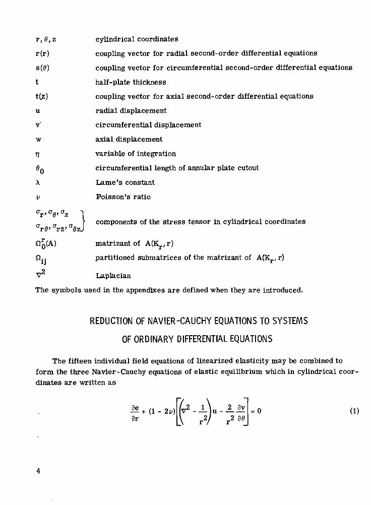
The fifteen individual field equations of linearized elasticity may be combined toform the three Navier-Cauchy equations of elastic equilibrium which in cylindrical coor-dinates are written as

^ + (1 - 2v)2 36

= 0 (1)

r 39= 0

-^ + (1 - 2z,)V2w = 0dz

(2)

(3)

where the body forces are assumed to be zero and the dilatation is

e - du j 1 3v H u + 3w3r r 30 r 3z

(4)

The stress-displacement relations, obtained by substituting the strain-displacementrelations into Hooke's law, can be expressed in the following form:

a =3r

(5)

(6)

<r =z 3z

(7)

r 30 3r(8)

rz \3r(9)

, /3v _1 3w\3z r 30

(10)

For a finite geometry body with circular boundaries, we construct three sets ofparallel lines in the direction of the coordinates as shown in figure 1. Approximatesolutions of equations (1) to (3) can then be obtained by developing solutions of ordinary 'differential equations along the radial, circumferential, and axial lines, respectively.For equation (1), we define the displacements along the radial lines as UpUg, . . . ,u,.The derivatives of the circumferential displacements on these lines with respect to 0

l = N6xNZ

m =NZxNR

n = NRxN6

M;ircumferentiallines

Radial lines

Figure 1. - Sets of lines in direction of cylindrical coordinates.

are defined as v| 2, • v| , and the derivatives of the axial displacements withrespect to z are defined as w ,, wL. These displacements and deriva-tives can then be regarded as functions of the radius only, since they are variables onradial lines. K these definitions are used, the ordinary differential equation along ageneric, radial line ij (a double subscript is used here for simplicity of writing) of fig-ure 1 may be written as

Ai + l^ii.!iidr r dr

(1 - 2v)2(1 - v)

u.. +r h.

2(1 - ,;)= 0 (U)

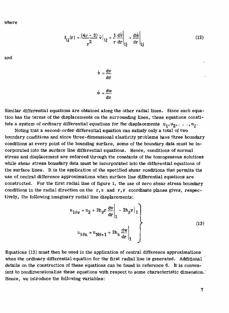
where

r dr+ dw

„ dr(12)

and

v = d

w = dwdz

Similar differential equations are obtained along the other radial lines. Since each equa-tion has the terms of the displacements on the surrounding lines, these equations consti-tute a system of ordinary differential equations for the displacements u^vug,. . . ,u^.

Noting that a second-order differential equation can satisfy only a total of twoboundary conditions and since three-dimensional elasticity problems have three boundaryconditions at every point of the bounding surface, some of the boundary data must be in-corporated into the surface line differential equations. Hence, conditions of normalstress and displacement are enforced through the constants of the homogeneous solutionswhile shear stress boundary data must be incorporated into the differential equations ofthe surface lines. It is the application of the specified shear conditions that permits theuse of central difference approximations when surface line differential equations areconstructed. For the first radial line of figure 1, the use of zero shear stress boundaryconditions in the radial direction on the r, z and r,0 coordinate planes gives, respec-tively, the following imaginary radial line displacements:

U10e = U 2 V - 2Vli(13)

Equations (13) must then be used in the application of central difference approximationswhen the ordinary differential equation for the first radial line is generated. Additionaldetails on the construction of these equations can be found in reference 6. It is conven-ient to nondimensionalize these equations with respect to some characteristic dimension.Hence, we introduce the following variables:

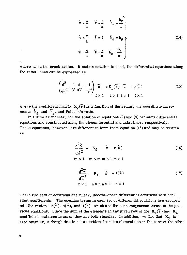
r= h =a a a

/v/ TTv =- h =

~ w ~ Z ~ Zw = - ^ z=- h = —a a a

(14)

^^r-— u = K ( r ) u + r ( r )

where a is the crack radius. If matrix notation is used, the differential equations alongthe radial lines can be expressed as

(15)

where the coefficient matrix K r(r) is a function of the radius, the coordinate incre-ments h- and hz, and Poisson's ratio.

In a similar manner, for the solution of equations (2) and (3) ordinary differentialequations are constructed along the circumferential and axial lines, respectively.These equations, however, are different in form from equation (15) and may be writtenas

v s (0 ) (16)

m x l m x m m x l m x l

= Kz w + t ( z )dz2 Z

n x l n x n n x l n x l

(17)

These two sets of equations are linear, second-order differential equations with con-stant coefficients. The coupling terms in each set of differential equations are groupedinto the vectors r(i-), s(??), and t('z), which are the nonhomogeneous terms in the pre-vious equations. Since the sum of the elements in any given row of the K(r ) and Kcoefficient matrices is zero, they are both singular. In addition, we find that Kg isalso singular, although this is not as evident from its elements as in the case of the other

coefficient matrices. A detailed listing of equations (15) to (17) may be found in refer-ence 6.

SOLUTION OF THE SYSTEMS OF ORDINARY DIFFERENTIAL EQUATIONS

The details of a solution technique for the type of simultaneous ordinary differentialequations given by equations (15) are discussed in appendix A. For the case r * 0, thesolution vector for the radial displacement is

u ( r ) =4- n n ( r ) [FJ + B^r )]+i O12(r) [k + B2(r)] (18)r r

Z x 1 Z x Z Z x 1 ix1 ix l lx1 lx 1

where

= r ur-rinitial

-~ Jr/~ „

r =r initial

and J71^('r ) and f212(^') are infinite matrix integral series whose definitions and evalu-ation are discussed in appendix A. Vectors B- , ( r )and B2(r) represent particularsolutions of equations (15), and they are given by

t

l(^) = - J~rinitial

i*

(n22 " n2lnllnr initial

while vectors Fj and F2 are initial value vectors whose evaluation from given bound-ary conditions is discussed in appendix C. Differentiating equation (18) with respect tor yields

u ( r ) =

Z x 1 z x Zr2

fx. I Z x 1 Z x 1

f (r) L O (r\Ct\t\ \ l . ) — —— &£ 4 n \ I ^

^^ ~2rZ X Z Z X Z Z x l Z x l

[F2 + B 2 ( r ) ]

(21)

where O2l (r) and O22 ) are ma*rix integral series similar to O i j C ) and fiiFor differential equations of the type given by equations (16) and (17), a detailed and

analogous solution procedure is discussed in appendix B. As a result of this develop-ment, the circumferential displacement vector may be written as

(22)

where and are matrix functions:

A n(0) = (23)

(24)

4/2 i,The matrix K/ is defined as a matrix whose square is equal to K0. Vectors v(0)and v (0) are initial value vectors whose evaluation from given boundary conditions isdiscussed in appendix C. Vectors Bg(^) and BAH) represent particular solutions ofequations (16) and are given by

SX

/ drj (25)

B4(0) = / AII(TJ)S(TJ) (26)

Differentiating equation (22) with respect to !) gives

v ( 0 ) =K0A1 2(0)[v(0)+ B3(7f)] + Au (27)

A solution vector similar to equation (22) may be constructed for equations (17) whichdefines the axial displacements. Since r(rj) in equations (19) and (20) is unknown, we

10

start the solution of the problem by assuming values of v, dv/dr , dw/dr, v, dv/dr,and dw/di- along the radial lines. The initial values of these required quantities weretaken to be zero in this report. Then equations (18) and (21) will give the first estimatefor the vectors u ( i - ) ^ 'and u("rr • It is assumed, of course, that vectors F^ andFO are known or can be found from given boundary conditions. Using these calculatedvalues of u (r )' ' and u (i- )^ ' we can evaluate the vector ^ (9 r where we must usesimilarly assumed values of dw/d'e and dw/d7> along the circumferential lines.Equations (22) and (27) give the first values of v^ r1' and v (6> )' '. First values of~ /~ \(1) ~ /~ (1}w ( z )v ' and w ( z )v ' can then be calculated by using the first estimates of the radial andcircumferential displacements and their derivatives in the coupling vector t(z )^ '. Atthis point we return to equations (18) and (21) and calculate the second values of u(i- rand u ( i- r based on the first values of the circumferential and axial solutions.

K the values of u( r )^ , u(r)^ , v(1?)H vd?)^, w(z )H and w(z )^ 1 ^ convergewith the repetition of this procedure, an approximate solution of a given problem will bedetermined. In general, the convergence rate for these successive calculations is de-pendent on the accuracy to which the matrix functions A. . and the matrix integral ser-ies J2, • can be evaluated. Sufficiently large errors in these matrix variables will leadto divergence in the successive approximation calculations.

Since the coupling vectors r(r'), s(1?), and t ( z ) involve displacements and theirderivatives defined only at the nodes, finite difference calculus must be used in evaluat-ing their elements. Hence, all the particular integrals are calculated by a suitablenumerical integration technique.

Once the displacement field in the bar has been calculated and the successive ap-proximation procedure has converged, the normal stress distributions along the threesets of parallel lines can be obtained from

(28)lines Along radial

lines

+ X ( u + w ) A 1 . rv 'Along circumfer-Along circumfer- .. , ,.& ential linesential lines

(X + 2G)(w )Along ax.al + X + + (30)

Unes /Along axiallines

11

Note that these equations involve only derivatives that can be analytically evaluated. Theshear stresses at each node can be calculated from equations (8) to (10), but finite dif-ference approximations must be used for the required displacement gradients.

NUMERICAL RESULTS

Solid Cylindrical Bar with Penny-Shaped Crack

Figure 2 shows a cylindrical bar containing a penny-shaped crack and loaded by auniform normal stress distribution. For problems with axisymmetric geometry, thecircumferential displacement is inherently zero at every point and all the remainingvariables are independent of the circumferential coordinate 0. The two sets of parallel

^-Penny-shaped crack:radius = a; v = 1/3 ^

Figure 2. - Solid cylindrical bar with penny-shaped crack.

12

lines needed for the solution of this problem are also shown in this figure. Note that thecrack edge is assumed to be midway between adjacent nodes, specifying normal stressand displacement boundary conditions, respectively.

The solution of this problem was obtained by using two different sets of lines alongthe coordinate axes so that the convergence of the finite difference approximations couldbe checked. The successive approximation procedure required for decoupling the twosets of ordinary differential equations was terminated when the difference between sue-

f*

cessively calculated displacements at every point was less than a preset value (10~ ).Selected results from these calculations are shown in tables I to V and figures 3 to 7. -For easy comparison of data, some of these figures include Sneddon's results for an

TABLE I. - NONDIMENSIONALIZED RADIAL DISPLACEMENTS Eu/cQa

FOR SOLID CYLINDRICAL BAR WITH PENNY-SHAPED CRACK

UNDER UNIFORM NORMAL TENSION

[a = 1. 0, b = 1. 77, L = 1. 68 (16 axial and 13 radial lines)]

z

0.00.28.56

.841.121.401.68

7

0.000

0.000

\

0.235

-0.168-.080-.045-.038-.039-.034-.006

0.471

-0.333-.153-.091-.083-.085-.074-.023

0.706

-0.488-.217-.149-.142-.142-.124-.058

0.941

-0.579-.297-.239-.223-.214-.188-.114

1.06

-0.609-.371-.300-.273-.255-.224-.150

1.294

-0.653-.529-.433-.379-.344-.303-.233

1.530

-0.705-.639-.549-.482-.435-.388-.325

1.770

-0.773-.725-.646-.580-.530-.483-.425

infinite solid (ref. 9). The data of figure 3 clearly show the advantage of the line methodover other numerical solutions. A relatively coarse grid of nine axial and nine radiallines gave almost identical results to those obtained by using a 16 by 13 grid. Since thebar is of finite size, the crack opening displacement is expected to be higher thanSneddon's solution. Consistency of the results with this conclusion is obvious fromfigure 6. It is noteworthy that the results correspond to elliptical crack profiles in allcases. The maximum dimensionless crack opening is plotted for several crack to cyl-inder radius ratios in figure 7. The data from figure 6 match the results of Sneddonand Welch (ref. 13) very closely, and, as expected, the maximum crack opening isslightly higher for finite length cylinders.

Figure 5 shows the stress distribution normal to the crack plane as a function of thedistance from the crack edge. As shown by Sneddon for an infinite solid, this stress

13

TABLE II. - NONDIMENSIONALIZED AXIAL DISPLACEMENTS

Ew/aQa FOR SOLID CYLINDRICAL BAR WITH

PENNY-SHAPED CRACK UNDER

UNIFORM NORMAL TENSION

[a = 1.0, b = 1. 77, L = 1. 68 (16 axial and 13 radial lines)]

r

0.000.235.471.706.941

1.0601.2941.5301.770

r>*>

z

0.000

1.3941.3511.219

.973

.515

.000

1

I

0.280

1.5441.4951.3591.113

.746

.542

.384

.334

.291

0.560

1.6461.5951.4721.2731.029

.913

.758

.673

.610

0.840

1.7661.7221.6221.4731.3021.2211.090

.999

.935

1.120

1.9281.8921.8121.6961.5651.5021.3901.3041.245

1.400

2.1262.0972.0291.9331.8231.7681.6701.5921.535

1.680

2.3292.3062.2502.1672.0722.0241.9371.8661.812

TABLE m. - NONDIMENSIONALIZED RADIAL STRESS ar/vQ FOR

SOLID CYLINDRICAL BAR WITH PENNY-SHAPED CRACK

UNDER UNIFORM NORMAL TENSION

[a = 1. 0, b = 1. 77, L = 1. 68 (16 axial and 13 radial lines)]

f**Jz

0.00.28.56.84

1.121.401.68

r

0.000

-1.060-.479-.148

.0211

.127

.246

.470

0.235

-1.043-.451-.141

.0144

.116

.230

.429

0.471

-1.017-.375-.123

.002

.093

.193

.352

0.706

-0.883-.270-.124-.0251

.058

.142

.247

0.941

-0.522-.262-.155-.058

.023

.088

.136

1.060

1.134-.138-.150-.065

.009

.064

.085

1.244

0.376-.095-.113-.056-.004

.028

.008

1.530

0.116-.017-.044-.026-.003

.012-.021

1.770

0.000

14

TABLE IV. - NONDIMENSIONALIZED CIRCUMFERENTIAL STRESS

FOR SOLID CYLINDRICAL BAR WITH PENNY-SHAPED CRACK

UNDER UNIFORM NORMAL TENSION

[a = 1.0, b = 1. 77, L = 1. 68 (16 axial and 13 radial lines)]

z

0.00.28.56.84

1.121.401.68

r

0.000

-1.060-.479-.148

.021

.127

.246

.470

0.235

-1.061-.461-.138

.023

.124

.23

.45

0.471

-1.047-.401-.106

.032

.120

.218

.401

0.706

-0.986-.291-.055

.047

.113

.191

.333

0.941

-0.790-.112

.011

.062

.104

.160

.257

1.060

0.909.108.049.067.099.144.220

1.294

0.125.015.037.062.086.116.154

1.530

-0.020-.023

.022

.055

.075

.096

.112

1.770

-0.108-.051

.024

.057

.064

.072

.089

TABLE V. - NONDIMENSIONALIZED AXIAL STRESS <JZ/VQ FOR

SOLID CYLINDRICAL BAR WITH PENNY-SHAPED CRACK

UNDER UNIFORM NORMAL TENSION

[a = 1. 0, b = 1. 77, L = 1. 68 (16 axial and 13 radial lines)]

rv

z

0.00.28.56.84

1.121.401.68

r^jr

0.000

0.000.095.277.515.736.900.999

0.235

0.000.093.295.542.759.915.998

0.471

0.000. 146.386.624.808.933.999

0.706

0.000.319.592.770.885.960.999

0.941

0.000.874.950.957.972.990

1.000

1.060

3.3201.5131.1501.0411.0101.003.999

1.294

1.5121.3651.23Q1.1221.0591.022

.995

1.530

1.2061.2011.1861.1361.0821.036.993

1.770

0.9891.0821.1721.1591.0921.037

.990

15

2.5

2.0

1.5

1.0

.50

0'

hr = 0.1176

hz = 0.140

I

2.5

2.0

1.5

1.0

.50

0

(a) Dimensionless axial displacement distribution (16 by 13grid).

v = ] / 3

hr = 0.222

hz = 0.210

.4 1.2 1.6 1.8

(b) Dimensionless axial displacement distribution <9 by 9 grid).

Figure 3. - Dimensionless axial displacement distributionfor solid cylindrical bar with penny-shaped crack.

distribution should approach infinity near the crack edge as the inverse square root ofthe distance from the crack edge. Establishment of this type of singularity is, however,difficult when numerical methods are used because values of the normal stress areneeded within a distance of 0.05 a or less from the crack tip. For the range of i-shown in figure 5, this inverse square root singularity is not defined. However, for therange shown, the obtained stress curve closely resembles Sneddon's solution (ref. 15).As expected, the absolute value of this stress is greater for a finite size bar than forSneddon's infinite solid. Tables I to V show selected results from the computer listings.The accuracy of the normal stress and displacement boundary conditions can easily benoted from the numerical data listed.

16

.70

.60

.50

.40

.30

.20

.10OT_

.235^

10° (a) Dimensionless radial displacement distribution (16 by 13grid).

.70

.60

.50

.40

.30

.20

.10

07 I.22 7

.40 .80 __ 1.2z

1.6 2.0

(b) Dimensionless radial displacement distribution (9 by 9 grid).

Figure 4. - Dimensionless radial displacement distributionfor solid cylindrical bar with penny-shaped crack.

r- |

|l\

ll \Crack | 1 \edge i I \location-! » \

a= 1.0

b= 1.77

L=1.68

v - U 3

V

hr= 0.1176

hz = 0.140

rSneddon's solution

I V >^/

— 1

ii. 1 1 1 i

v 1.0 1.2 1.4 1.6r

11.8

Figure 5. - Dimensionless axial stress distribution (16 by 13 grid)for solid cylindrical bar with penny-shaped crack at 7= 0.

17

•£

1.5

1.0

.5

1.77

2.2

1.8O O

c. &

0 .2 .6 1.0

Figure 6. - Dimensionless crack opening displacements forsolid cylindrical bars with penny-shaped cracks of variouslengths and radii.

1.4

Data from figure 6

Sneddon and Welch,v - 1/3, L - oo

Figure 7. - Dimensionless maximum crack opening asfunction of crack to cylinder radius ratio.

Annular Plate with Internal Surface Cracks

As a first attempt at the solution of a general three-dimensional problem in cylin-drical coordinates, the problem of figure 8 was investigated. In order to minimize thenumerical computations, we have assumed four symmetrically located internal surfacecracks. Because of the symmetric geometry and loading, only one-sixteenth of theoriginal plate has to be discretized. Figure 9 shows this region of interest and the as-sumed crack geometry. Note that nondimensionalization with respect to the outsideradius is more convenient in this case since the crack has two characteristic dimensions.

Displacement and normal stress distributions were calculated along the lines offigure 9 using a grid of 16 lines in all directions. Because of the relatively coarse gridinvolved, the results appear only in tabular form (tables VI to XI). It must be noted,however, that because of the unknown nature of the resulting solutions, the use of acoarse grid is always recommended in generating the first set of displacements. Sincethe construction of a general computer program for this problem requires a greatamount of effort, the results in tables VI to XI were calculated by using only one set oflines with NR = N6> = NZ = 4.

Tables VI to Vm contain the dimensionless displacement distributions. These re-sults show that below the crack plane the circumferential displacements are essentiallyzero while the maximum crack opening is at "e = z =0 and r^ 0. 25. Although bothradial and circumferential displacement fields are extensional, the axial displacementsare negative, which indicates a contraction in that direction. The calculated normal

18

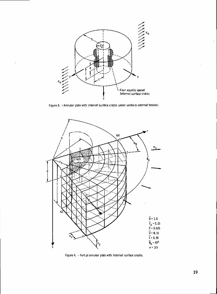
\-Four equally spacedinternal surface cracks

Figure 8. - Annular plate with internal surface cracks under uniform external tension.

t> = 1.0

70-0.25

0 = 0.625

d = 0.15

Figure 9. - Part of annular plate with internal surface cracks.

19

TABLE VI. - DDHENSIONLESS RADIAL DISPLACEMENTS

Eu/aQb FOR ANNULAR PLATE WITH INTERNAL

SURFACE CRACKS UNDER UNIFORM RADIAL

TENSION ON OUTSIDE SURFACE

«,deg

r

0.25 0.50 0.75 1.00

z = 0. 00

015

3045

0.435.940.168

1.240

0.671.890.992

1.026

0.786.896.968.994

0.930.998

1.0581.081

z = 0. 10

015

3045

0.506.907

1.0921.152

0.680.860.953.986

0.789.886.957.984

0.930.994

1.0551.076

"z = 0 . 2 00

15

3045

0.724.795.898.942

0.656.761.856.892

0.779.856.932.961

0.927.965

1.0481.073

z = 0 . 3 0

015

3045

0.716.752.815.845

0.659.727.809.843

0.769.845.926.957

0.915.978

1.0491.077

20

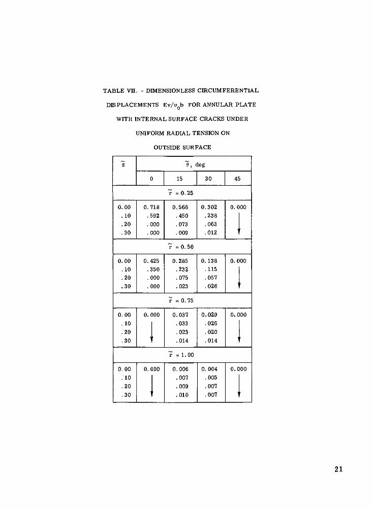
TABLE VII. - DIMENSIONLESS CIRCUMFERENTIAL

DISPLACEMENTS Ev/aQb FOR ANNULAR PLATE

WITH INTERNAL SURFACE CRACKS UNDER

UNIFORM RADIAL TENSION ON

OUTSIDE SURFACE

z ~d, deg

0 15 30 45

r =0.25

0.00.10.20.30

0.718.592.000.000

0.566.450.073.009

0.302.238.063.012

0.000

1

T

7 =0 .50

0.00.10.20.30

0.425.350.000.000

0.285.232.075.023

0.138.115.057.026

0.000

1T

r =0 .75

0.00. 10.20.30

0.000

V

0.037.033.023.014

0.029.026.020.014

0,000

1

r =1.00

0.00. 10.20.30

0.000

1T

0.006.007.009.010

0.004.005.007.007

0.000

r

21

TABLE VHI. - DIMENSIONLESS AXIAL DISPLACEMENTS

Ew/aQb FOR ANNULAR PLATE WITH INTERNAL

SURFACE CRACKS UNDER UNIFORM RADIAL

TENSION ON OUTSIDE SURFACE

fv

T "z

0.00 0.10 0.20 0.30

0=0°

0.25.50.751.00

0.000

11

-0.218-.108-.089-.076

-0.342-.217-.175-.152

-0.416-.322-.256-.226

"e =15°

0.25.50.751.00

0.000

1T

-0.098-.049-.075-.074

-0.216-.131-.154-.149

-0.336-.232-.237-.226

"e =30°

0.25.50.751.00

0.000

1t

-0.068-.040-.067-.075

-0.167-.106-.141-.152

-0.281-.195-.222-.231

6 =45°

0.25.50.751.00

0.000

1f

-0.061-.039-.065-.075

-0. 153-.101-.137-.153

-0.262-.186-.218-.233

22

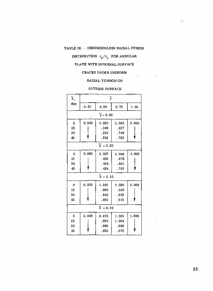
TABLE DC. - DEMENSIONLESS RADIAL STRESS

DISTRIBUTION <JT/VQ FOR ANNULAR

PLATE WITH INTERNAL SURFACE

CRACKS UNDER UNIFORM

RADIAL TENSION ON

OUTSIDE SURFACE

0,deg

r

,0.25 0.50 0.75 1.00

Is =0.00

0153045

0.000

1

T

0.020

.346

.293

.282

1.062.837.748.726

1.000

1

I

'z =0.20

0153045

0.000

1t

0.027

.405

.424

.424

1.048.872

.801

.783

1.000

1

Ifz =0.10

0153045

0.000

1\

1.305

.968

.840

.801

1.026.980.932.915

1.000

1

"z = 0.30

0153045

0.000

1T

0.872

.950

.966

.956

1.0051.004.986.975

1.000

1T

23

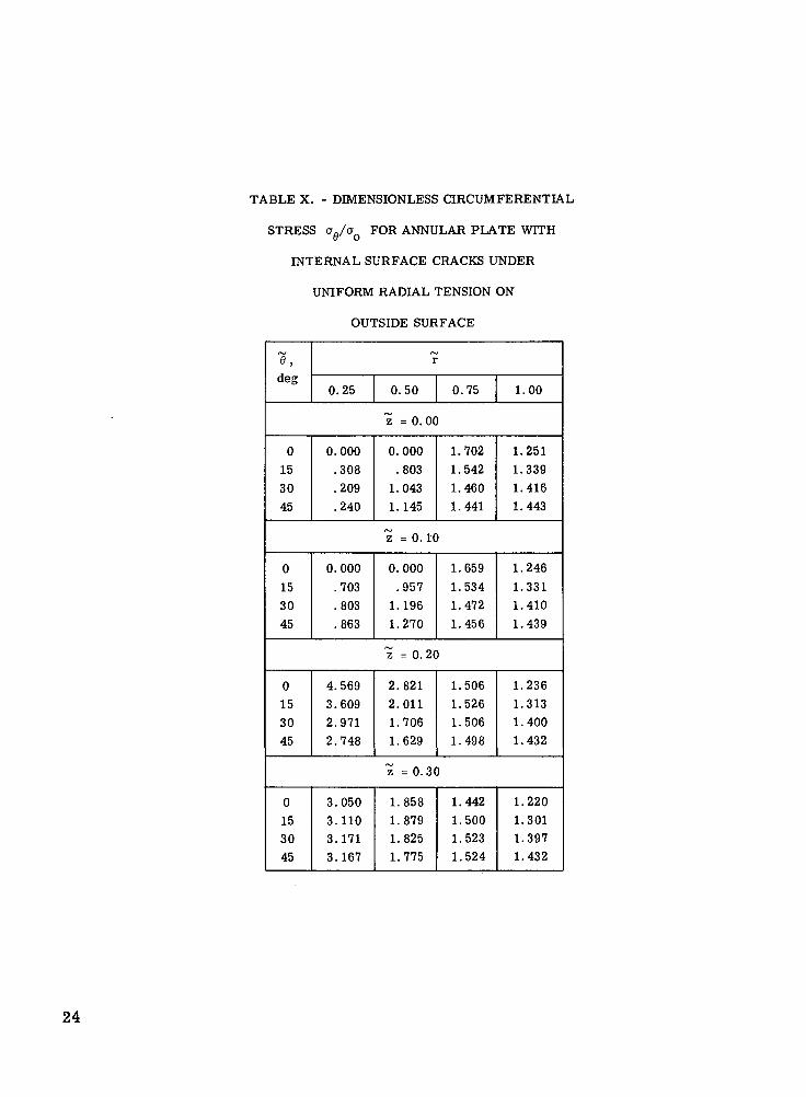
TABLE X. - DIMENSIONLESS CIRCUMFERENTIAL

STRESS afl/a FOR ANNULAR PLATE WITHu O

INTERNAL SURFACE CRACKS UNDER

UNIFORM RADIAL TENSION ON

OUTSIDE SURFACE

e,deg

"r

0.25 0.50 0.75 1.00

z = 0. 00

0

15

30

45

0.000.308.209.240

0.000.803

1.0431.145

1.7021.5421.4601.441

1.2511.3391.4161.443

z = 0. 10

0

15

30

45

0.000.703.803.863

0.000.957

1.1961.270

1.6591.5341.4721.456

1.2461.3311.4101.439

z =0 .20

015

3045

4.5693.6092.9712.748

2.8212.0111.7061.629

1.5061.5261.5061.498

1.2361.3131.4001.432

z = 0 . 3 0

0153045

3.0503.1103.1713.167

1.8581.8791.8251.775

1.4421.5001.5231.524

1.2201.3011.3971.432

24

TABLE XI. - DIMENSIONLESS AXIAL STRESS az/aQ

FOR ANNULAR PLATE WITH INTERNAL SURFACE

CRACKS UNDER UNIFORM RADIAL TENSION

ON OUTSIDE SURFACE

r^i

e,deg

r

0.25 0.50 0.75 1.00

z =0 .00

015

3045

-1.974-.939-.631-.544

-1.049-.126

.041

.082

0.030.043.064.070

-0.014.040.060.062

z =0.10

0

15

3045

-1.59T-.867-.579-.487

-1.073-.210

.006

.055

0.028.032.053.059

-0.010.031.046.048

z = 0 . 2 0

0

15

3045

0.500-3.135-.077-.097

0.313-1.996

.070

.073

0.002-1.504

.039

.042

-0.004-1.310

.019

.020

z =0 .30

015

3045

0.000

111

0.000

11t

0.000

I '

0.000

1

25

stresses are summarized in tables IX to XI. It is expected that the circumferentialstress be the maximum tensile stress in the body since the crack plane is normal to thiscoordinate. The interaction between the hole and crack stress fields should also be mostpronounced at the inside radius; from this we conclude that the stress should be maxi-mum at that point. The results of table X seem to confirm these observations, althoughwe must also remember that the nodes are closer to the crack boundary below the cracksurface than along the radius.

Because of the use of a coarse grid, the numerical results for this example aresomewhat inaccurate in magnitude but they do indicate some previously unknown varia-tions in the stress field for this problem. This conclusion is possible in that the linemethod does not usually require a fine grid for good results as was shown in the previ-ous section. These results also demonstrate that the method of lines permits the com-putation of the displacement and stress fields for a general three-dimensional problem.

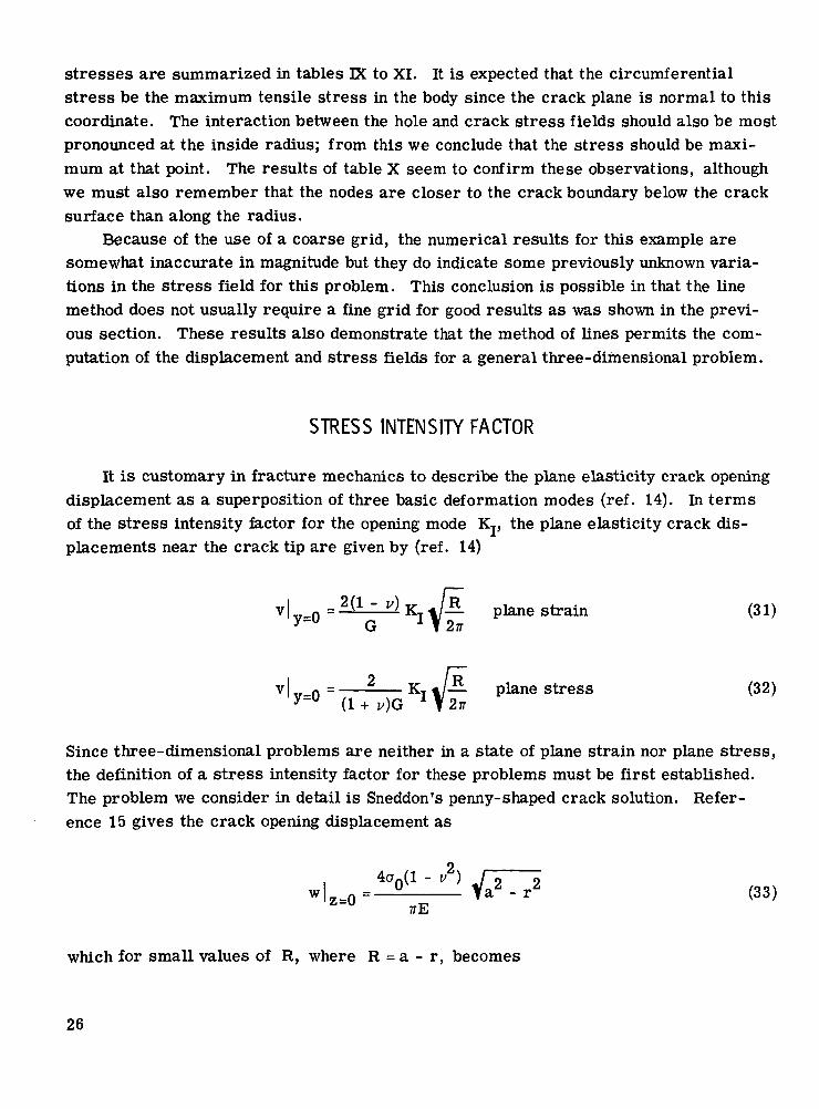
STRESS INTENSITY FACTOR

It is customary in fracture mechanics to describe the plane elasticity crack openingdisplacement as a superposition of three basic deformation modes (ref. 14). In termsof the stress intensity factor for the opening mode Kj, the plane elasticity crack dis-placements near the crack tip are given by (ref. 14)

= 2(* " ") KT t/— Plane strain (31)-° G I f 2?r

_ plane stress (32)2ir

Since three-dimensional problems are neither in a state of plane strain nor plane stress,the definition of a stress intensity factor for these problems must be first established.The problem we consider in detail is Sneddon's penny-shaped crack solution. Refer-ence 15 gives the crack opening displacement as

. 4crn(l - v2) J~<> ow z - 0 = — ~ Va 2 - r 2 (33)

Z~U 7TE

which for small values of R, where R = a - r, becomes

26

4or0(l - l/) ,w| 0 = — V2aR (34)

TrE

Note that adjustment of coordinates must be made between the equations quoted fromreferences 14 and 15. Paris and Sih (ref. 14) list the stress intensity factor for thisproblem as

O I—

(35)

In terms of this stress intensity factor, the crack opening displacement (eq. (34))becomes

w|z_0 = ̂ *SLL£J™**!±J*^J* (36)z~° l E M n G 1 T 2 7 T

Rearranging this equation in terms of the known dimensionless displacements(E/a0)(w/a) gives

z=0

_E_ w

Eao

(37)

where

Cj = ̂ " v > (38)E V27ra

Then a plot of equation (37) as \R/a — 0 gives the desired value of (E/<TQ)CjKj fromwhich an equivalent stress intensity factor for finite geometry cylinders can be calcu-lated. Note from equation (36) that the definition of Ky given in equation (35) impliesthe plane strain crack opening displacement of equation (31).

For problems in which the crack opening displacement varies in the thickness direc-tion, such as the annular plate with internal surface cracks, the stress intensity factorobtained previously will be a function of the thickness variable. However, if we were toaccount for the nonplane strain conditions near the surface by using equation (32) or a

27

corrected equation (31) for the definition of K,, the stress intensity factor would becomea constant across the thickness by definition. It should be noted that this description ofKj is completely arbitrary and its significance in three-dimensional elasticity theory isof doubtful value. However, values of Kj are still presented so that a comparison willbe possible between the calculated results and the published plane strain solutions(ref. 14).

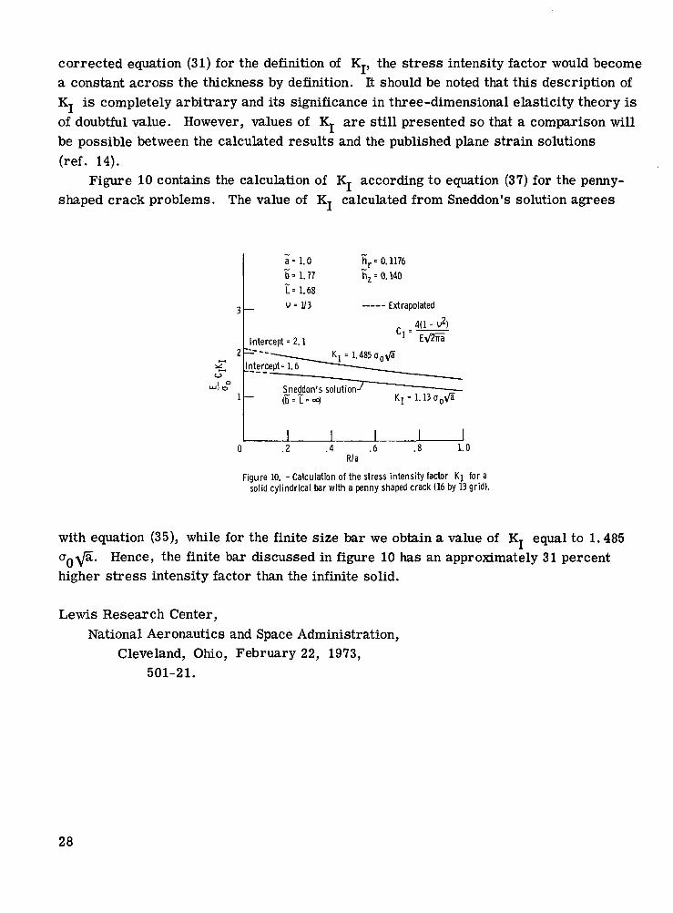
Figure 10 contains the calculation of K, according to equation (37) for the penny-shaped crack problems. The value of K calculated from Sneddon's solution agrees

2

a = 1.0

b=1.77

1=1.68

v-1 /3

Intercept = 2. 1

hr - 0. 1176h • 0. 140

---- Extrapolated

4(1 - v2)~

[ntercept -1.6

1.13o0Va

0 .2 .4R/a

.6 1.0

Figure 10. -Calculation of the stress intensity factor Kj forasolid cylindrical bar with a penny shaped crack (16 by 13 grid).

with equation (35), while for the finite size bar we obtain a value of Kj equal to 1. 485(TQ-^a. Hence, the finite bar discussed in figure 10 has an approximately 31 percenthigher stress intensity factor than the infinite solid.

Lewis Research Center,National Aeronautics and Space Administration,

Cleveland, Ohio, February 22, 1973,501-21.

28

APPENDIX A

SOLUTION OF SIMULTANEOUS DIFFERENTIAL EQUATIONS

WITH VARIABLE COEFFICIENTS

Noting that the differential operator of equations (15) can be written as d/di-[l/i- xd/d'r ("ru)], the following variables are introduced in order to obtain a system of first-order differential equations:

r dr

U« = r u., U9 = r u9, . . . , U, = r u

LA.r dr

In terms of these variables, equations (15) can be written as

!_d_

"r d i-

(Al)

where

= A( r ) U r ( r )dr

21 x 1 21x21 21 x 1 21 x 1

A ( r ) =21 x 21

0I x

rlI x i

0

I x ZJ

(A2)

(A3)

r ( r ) =21 x 1

I x 1

r ( r )I x 1

(A4)

Following the Peano-Baker form of integration (ref. 16), the solution of equation (A2) is

29

r1

U ( r ) = n n ( A ) u(°) + fin (A) / lnn(A) ^(TJ) drj (A5)

2 l x l 21*2121*1 2 1 X 2 1 2 1 X 2 1 2 l x l

where vector U(0) consists of the boundary values of (r u) and [l/r'd/d'r (r u)3 at theinitial value of r" which is taken as zero in this case. The matrizant of A(r*) is aninfinite matrix integral series given by

(A) = I + Afaj) dTjj + A(TJ2) drj2

dTJ2 A(»?I) * » ! + • • • (A6)

Substituting matrix A(r ) into equation (A6) leads to the following four matrix integralseries in terms of the coefficient matrix K(i-):

n ( r ) = I + I Tj I d77 I J _ K ( T j ) d 7 ] + . . . (A7)

/

r

11

olx I ix l ix l ix I

•r

n 1 9 ( r ) = i'12

x l lx II'JQ

"r /*Tj3 rnI TJ3d7J3 / -1 Kr(T?2)dT72 I

«/o 7?2 «A)(A8)

30

AI x Z Z x Z

rr• I -Jo "3

P2!

I *

+ . . . (A9)

Z x Z Z x Z Z x Z

pi rI — K (7]2) dr)2 I/ 77o /

»/0 «/0

(A10)

Z x Z Z x Z Z x Z Z x Z

An inspection of these equations shows that the following relations exist among thesefour matrix integral series:

~r dr

dr= n n ( r )K r ( r )

(All)

*r dr

dr

(A12)

From the definitions of these matrix series we can easily conclude that their initialvalues are

31

(A13)

= 1

Since the matrix series (A7) to (A10) are usually difficult to evaluate by performing theindicated integrations, the previous simultaneous matrix differential equations may besolved by a suitable numerical technique instead. The necessary initial conditions forthese numerical solutions are given by equations (A13). For the examples presented inthis report, the single step Runge-Kutta integration method was used to solve equa-tions (All) and (A12).

The particular integral of equation (A5) is written as

I x 1

B2(r)

I x 1

(A14)

In evaluating the inverse of fi by partitioning, the partitioned integrals (A 14) are givenby

/*T*

B1(r ) = - J nnn12( *? (A15)

B2(r ) =

r*j•r 1

rfa) (A16)

If it is assumed that r(r/) is known, the previous particular integrals can easily be eval-uated. When the partitioned form of the matrices is used, equation (A5) may be writtenas

32

r u

r dr

» =

f^f t^>

p21(r) «22(r_)

/

\

r u

r dr

r r~7l\

B 2 ( r ) j l(A17)

r=0

from which the solution vectors (18) and (21) can be directly constructed.It may be noted that for axisymmetric problems the following identities can be used

to evaluate the particular integrals:

-1

-1(A18)

These identities are obtained from noting that the inverse of the matrizant OQ (A) isgiven by

(A19)

when the coefficient matrix is of the form (A3) and the matrix K_ has constants for itselements.

33

APPENDIX B

SOLUTION OF SIMULTANEOUS DIFFERENTIAL EQUATIONS

WITH CONSTANT COEFFICIENTS

For the solution of equations (16) we introduce the following new variables:

V l = v l ' V2 = V2' • • • '

dv, dv2W ' ' '

dvm(Bl)

In terms of these variables, equations (16) can be written as a set of first-order differ-ential equations. Hence, we have

where

dVr*j

d0V + s ( 0 )

2m x 1 2m x 2m 2m x 1 2m x 1

2m x 2m

0 Im x m m x m

Kg 0_m x m m x m.

2m x lmx 1

(B2)

(B3)

(B4)

34

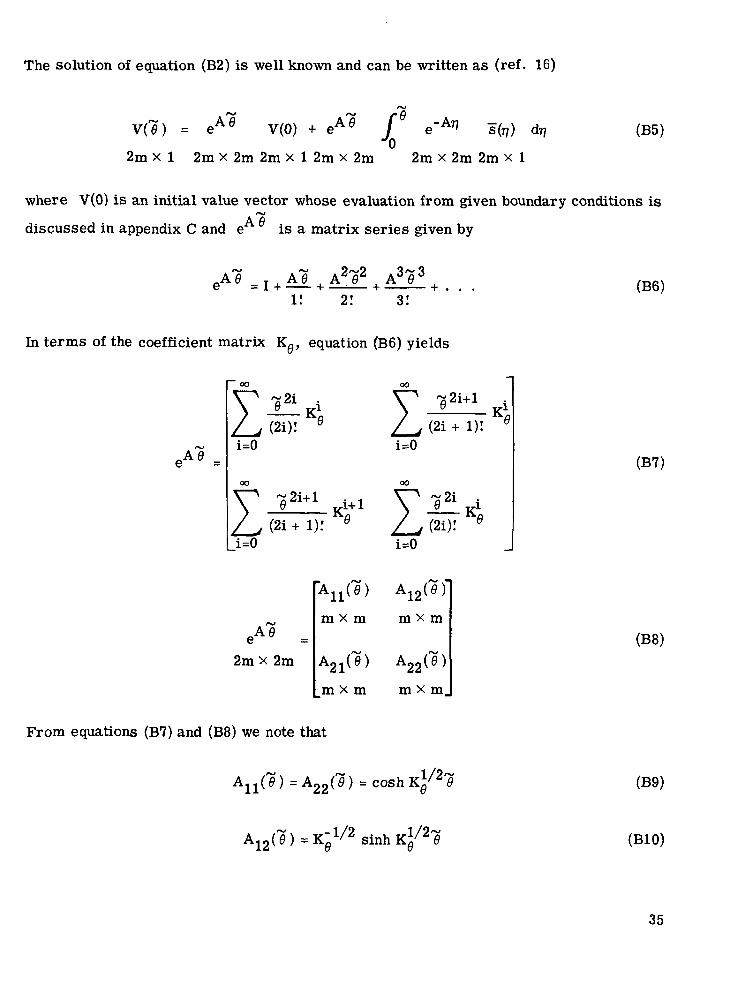
The solution of equation (B2) is well known and can be written as (ref. 16)

V(0) + eA° / e-™> s(r/) dr?

2m x 1 2m x 2m 2m x 1 2m x 2m 2m x 2m 2m x 1

(B5)

where V(0) is an initial value vector whose evaluation from given boundary conditions isA Sdiscussed in appendix C and e is a matrix series given by

1! 2!(B6)

In terms of the coefficient matrix K0, equation (B6) yields

i=0

00

y/^i=0

(2i + i): B

i=0 i=0

(B7)

2m x 2m

* */x/ /"" \A n (0 ) A1 2(e)m x m m x m

>21(0) A 22^ 6 ^

_m x m m x m.

<B8)

From equations (B7) and (B8) we note that

(B9)

(BIO)

35

(Bll)

1/2where K/ is a matrix whose square is equal to Kg. Noting that A..., and Aon areeven functions of ?) while A12 and A«^ are odd functions of 1) , the inverse of

becomes

.-A0-A12(0)

A22C0)

(B12)

A

Substituting equations (B8) and (B12) into the identity of e e • e = I yields

A2n(~e)- (B13)

m x m m x m m x m

Matrix functions (B9) and (BIO) may be evaluated for each value of the independent vari-able from the series definitions given in equation (B7). The truncation point in eachseries is determined by the required accuracy for the convergence of the successiveapproximation calculations. Equation (B13) may be used as a measure of this requiredaccuracy. However, for increasing values of 7) serious convergence difficulties mayarise and an impractically large number of terms must be calculated. In order to avoidthese computational difficulties, additive formulas for these matrix functions may beobtained from using the identity of

= eA^+'Sg)

(B14)

In terms of the submatrices A(6 ), this identity yields the following equations:

A21< (B15)

A12(e1 (B16)

The advantage of using equations (B7), (B15), and (B16) is that the solution of an eigen-value problem is not required. Alternate methods for the evaluation of these matrixfunctions using the solution of the determinantal equation are discussed in reference 6.

The particular integrals of equations (16) are constructed in a similar manner to

36

those listed in equations (A15) and (A16). The analogous particular integrals are

m x l

s(rj)

m x m m x 1

(B17)

r*s

/

QA n (0) 8(77) (B18)

m x 1 m x m m x 1

Assuming that 3(77) is known, these integrals can easily be evaluated. When the parti-tioned form of the matrices is used, solution vector (B5) for the circumferential differ-ential equations may be written as

A n(0) A12(0)i

A21(0) A2 2(0)

which when expanded yields equations (22) and (27).

(B19)

37

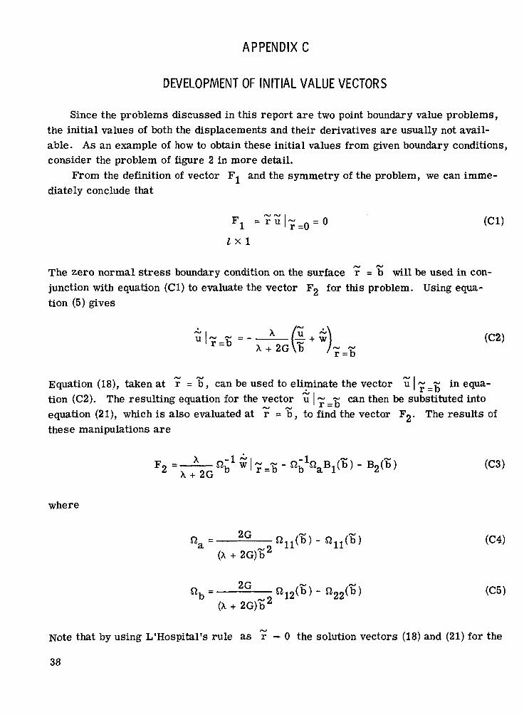
APPENDIX C

DEVELOPMENT OF INITIAL VALUE VECTORS

Since the problems discussed in this report are two point boundary value problems,the initial values of both the displacements and their derivatives are usually not avail-able. As an example of how to obtain these initial values from given boundary conditions,consider the problem of figure 2 in more detail.

From the definition of vector F* and the symmetry of the problem, we can imme-diately conclude that

I x 1

The zero normal stress boundary condition on the surface r = b will be used in con-junction with equation (Cl) to evaluate the vector F2 for this problem. Using equa-tion (5) gives

/~ . \(C2)

+ 2G\b

Equation (18), taken at r = b, can be used to eliminate the vector u | ~ _y in equa-tion (C2). The resulting equation for the vector u ~_r can then be substituted intoequation (21), which is also evaluated at r =b, to find the vector Fg. The results ofthese manipulations are

F« =—-— nr w |~r - nr n_B. , (b) - B9(b) (cs)* X + 2G ° ° ° a i

where

(X + 2G)b2

(X + 2G)b2

(C4)

(C5)

Note that by using L'Hospital's rule as r - 0 the solution vectors (18) and (21) for the

38

problem in figure 2 become

u (0) = 0

(C6)

Since for axisymmetric problems the circumferential displacements are inherentlyzero, the initial value vectors of the axial solutions will be considered next. An analo-gous solution to equations (22) and (27) along the z-directional lines can be written as

A ( z ) A ( z )n 12

(C7)

If the number of axial lines falling over the crack surface is denoted as NIC and thosefalling outside as NOC, the zero normal stress condition over the crack face and thesymmetry condition in the crack plane result in the following equations:

w(0) = -

NICx 1X + 2 G \ r / ~ = Q

inside crack

(C8)

NOC x 1 outside crack

(C9)

Assuming that on the face z = L we have a uniform tensile stress offigure 2, the normal stress boundary condition on this plane gives

as shown in

w (L ) = •X + 2G X + 2G

nx 1

(CIO)

This vector can be suitably partitioned into vectors w a (L) and w«(L) . For conven-NIC x 1 NOC x 1

ience of matrix manipulations, we construct the vectors as follows:

39

w(0)nx 1

w(0)nx 1

NICx 1

'5/3NOCx 1

NICx 1

6/3NOCx 1

(Cll)

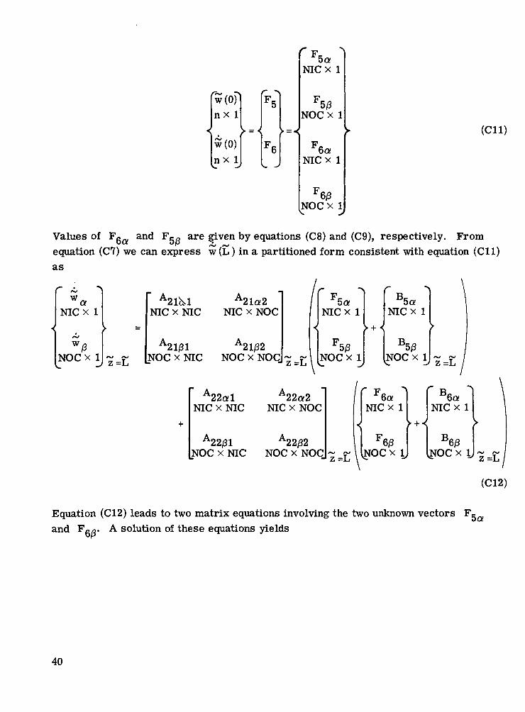
Values of Fga and Fgg are given by equations (C8) and (C9), respectively. Fromequation (C7) we can express w (L) in a partitioned form consistent with equation (Cll)as

I, -, r > \w«

NICx 1

W o

NOCx 1 z=L

A A01x1 *^'

NIC x NIC NIC x NOC

A21/31 A21j32NOC x NIC NOC x NOQ z=L

NICX 1

NOCx 1

NICx 1

NOCx 1

NIC x NIC NIC x NOC

22/31NOC x NIC NOC x NOC z=L

NICx 1

r-w ^

z=L

NICx 1

£TOCx

(C12)

Equation (C12) leads to two matrix equations involving the two unknown vectors Fgand F. A solution of these equations yields

40

/>*/

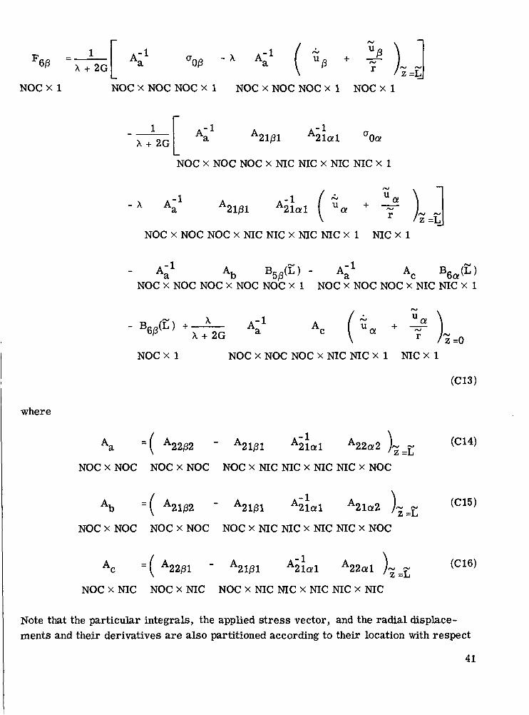
u

X + 2G

NOCx 1z=L

NOC x NOC NOC x 1 NOC x NOC NOG x 1 NOC x 1

X + 2G Si A21/31 A21al CTOar

NOC x NOC NOC x NIC NIC x NIC NIC x 1

- X A-1A21/31 A21al UQI +

NOC x NOC NOC x NIC NIC x NIC NIC x 1 NIC X 1

1 A /~ ^ -1 A na b ^5/3^' ~ a c 6

NOC x NOC NOC x NOC NOC x 1 NOC x NOC NOC x NIC NIC x 1

,-1 u aX + 2G r / z=0

NOCx 1 NOC x NOC NOC x NIC NIC x 1 NIC x 1

where

(C13)

A22/32

NOC x NOC NOC x NOC NOC x NIC NIC x NIC NIC x NOCz=L

(C14)

-( A21/32 A21/31 A21al A21a2 z=LNOC x NOC NOC x NOC NOC x NIC NIC x NIC NIC x NOC

•( A2lal A22al =LNOC x NIC NOC x NIC NOC x NIC NIC x NIC NIC x NIC

(CIS)

(C16)

Note that the particular integrals, the applied stress vector, and the radial displace-ments and their derivatives are also partitioned according to their location with respect

41

to the crack.The crack opening displacement is given by

A + 2G

NICx 1

- X Au

u« +a

z=LNIC x NIC NIC x 1 NIC x NIC NIC x 1 NIC x 1

- B L - lA21al A22a221a2 5

NIC x 1 NIC x NIC NIC x NOC NOC x 1 NIC x NIC NIC x NIC NIC x 1

X + 2GA2lQil A22al | ua +

uQ!

z=0NIC x NIC NIC x NIC NIC x 1 NIC x 1

_1 -i

NIC x NIC NIC x NOC NOC x 1 NIC x NIC NIC x NOC NOC x 1

B6/3(L) (C17)

where Fgg is given by equation (C13). Although the matrix A2j(L) is singular, thepartitioned matrices are not. In calculating the previous equations the indeterminateterms at r = 0 must be carefully considered.

42

REFERENCES

1. Lur'e, A. I.: Three-Dimensional Problems of the Theory of Elasticity. IntersciencePublishers, 1964.

2. Ayres, David J.: A Numerical Procedure for Calculating Stress and DeformationNear a Slit in a Three-Dimensional Elastic-Plastic Solid. NASA TM X-52440, 1968.

3. Cruse, T. A.: The Direct Potential Method in Three-Dimensional Elastostatics.Rep. SM-13, Carnegie-Mellon University (NASA CR-66673), June 1968.

4. ZienMewicz, Olgierd C.: The Finite Element Method in Engineering Science.Second ed., McGraw-Hill Book Co., Inc., 1971.

5. Hartranft, R. J.; and Sih, G. C.: The Use of Eigenfunction Expansions in the Gen-eral Solution of Three-Dimensional Crack Problems. J. Math. Mech., vol. 19,no. 2, Aug. 1969, pp. 123-138.

6. Gyekenyesi, John P.: Solution of Some Mixed Boundary Value Problems of Three-Dimensional Elasticity by the Method of Lines. Ph.D. Thesis, Michigan StateUniv., 1972.

7. Faddeeva, V. N.: The Method of Lines Applicable to Some Boundary Problems.Trudy Mat. Inst. Steklov, vol. 28, 1949, pp. 73-103.

8. Irobe, Makoto: Method of Numerical Analysis for Three-Dimensional Elastic Prob-lems. Proceedings of the 16th Japan National Congress of Applied Mechanics.Central Scientific Publishers, Tokyo, 1968, pp. 1-7.

9. Sneddon, I. N.: The Distribution of Stress in the Neighbourhood of a Crack in anElastic Solid. Proc. Roy. Soc. (London), Ser. A, vol. 187, no. 1009, Oct. 22,1946, pp. 229-260.

10. Hartranft, R. J.; and Sih, G. C.: An Approximate Three-Dimensional Theory ofPlates with Application to Crack Problems. Tech. Rep. 7, Lehigh Univ. (NASACR-103211), May 1968.

11. Cruse, T. A.; and Van Buren, W.: Three-Dimensional Elastic Stress Analysis ofa Fracture Specimen with an Edge Crack. Rep. SM-21, Carnegie-Mellon Uni-versity, Dept. of Mech. Eng., January 1970.

12. Gyekenyesi, John P.; Mendelson, Alexander; and Kring, Jon: Three-DimensionalElastic Stress and Displacement Analysis of Tensile Fracture Specimens Contain-ing Cracks. NASA TN D-7213, 1973.

43

13. Sneddon, I. N.; and Welch, J. T.: A Note on the Distribution of Stress in a CylinderContaining a Penny-Shaped Crack. Int. J. Eng. Sci., vol. 1, 1963, pp. 411-419.

14. Paris, P. C.; and Sih, G. C.: Stress Analysis of Cracks. Fracture ToughnessTesting and Its Applications. Spec. Tech. Publ. No. 381, ASTM, 1965, pp. 30-83.

15. Sneddon, I. N.: Crack Problems in the Mathematical Theory of Elasticity. NorthCarolina State College, Dept. of Mathematics and Eng. Res., 1961.

16. Frazer, R. A.; Duncan, W. J.; and Collar, A. R.: Elementary Matrices andSome Applications to Dynamics and Differential Equations. Cambridge UniversityPress, 1938.

" NASA-Langley, 1973 32 E-7258

Page Intentionally Left Blank

NATIONAL AERONAUTICS AND SPACE ADMINISTRATION

WASHINGTON, D.C. 2O546

OFFICIAL BUSINESS

PENALTY FOR PRIVATE USE S3OO SPECIAL FOURTH-CLASS RATEBOOK

POSTAGE AND FEES PAID

SPACE ADMINISTRATION451

POSTMASTER : If Undeliverable (Section 158Postal Manual) Do Not Return

"The aeronautical and space activities of the United States shall beconducted so as to contribute . . . to the expansion of human knowl-edge of phenomena in the atmosphere and space. The Administrationshall provide for the widest practicable and appropriate disseminationof information concerning its activities and the results thereof."

—NATIONAL AERONAUTICS AND SPACE ACT OF 1958

NASA SCIENTIFIC AND TECHNICAL PUBLICATIONSTECHNICAL REPORTS: Scientific andtechnical information considered important,complete, and a lasting contribution to existingknowledge.

TECHNICAL NOTES: Information less broadin scope but nevertheless of importance as acontribution to existing knowledge.

TECHNICAL MEMORANDUMS:Information receiving limited distributionbecause of preliminary data, security classifica-tion, or other reasons. Also includes conferenceproceedings with either limited or unlimiteddistribution.

CONTRACTOR REPORTS: Scientific andtechnical information generated under a NASAcontract or grant and considered an importantcontribution to existing knowledge.

TECHNICAL TRANSLATIONS: Informationpublished in a foreign language consideredto merit NASA distribution in English.

SPECIAL PUBLICATIONS: Informationderived from or of value to NASA activities.Publications include final reports of majorprojects, monographs, data compilations,handbooks, sourcebooks, and specialbibliographies.

TECHNOLOGY UTILIZATIONPUBLICATIONS: Information on technologyused by NASA that may be of particularinterest in commercial and other non-aerospaceapplications. Publications include Tech Briefs,Technology Utilization Reports andTechnology Surveys.

Details on the availability of these publications may be obtained from:

SCIENTIFIC AND TECHNICAL INFORMATION OFFICE

N A T I O N A L A E R O N A U T I C S A N D S P A C E A D M I N I S T R A T I O NWashington, D.C. 20546