Embed Size (px)
Citation preview

1
A Working Knowledge of Computational Complexity
for an Optimizer
ORF 363/COS 323
Instructor: Amir Ali AhmadiTAs: Y. Chen, G. Hall, J. Ye
Fall 2014
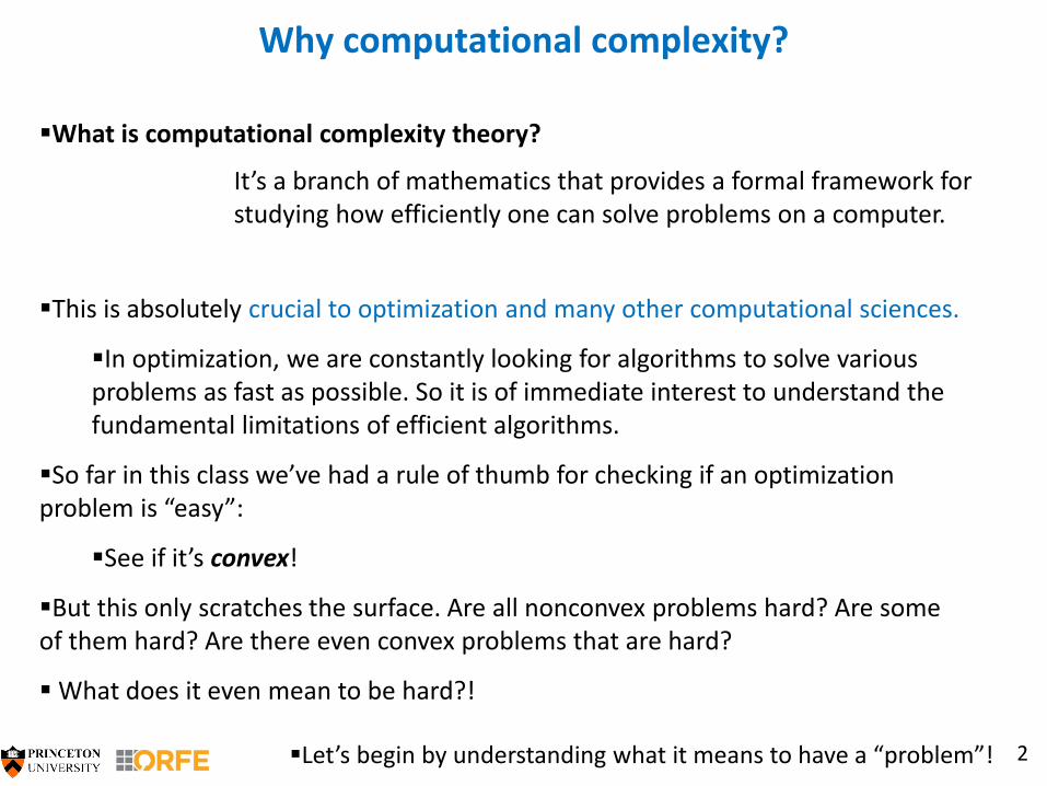
Why computational complexity?
2
What is computational complexity theory?
It’s a branch of mathematics that provides a formal framework for studying how efficiently one can solve problems on a computer.
This is absolutely crucial to optimization and many other computational sciences.
In optimization, we are constantly looking for algorithms to solve various problems as fast as possible. So it is of immediate interest to understand the fundamental limitations of efficient algorithms.
So far in this class we’ve had a rule of thumb for checking if an optimization problem is “easy”:
See if it’s convex!
But this only scratches the surface. Are all nonconvex problems hard? Are some of them hard? Are there even convex problems that are hard?
What does it even mean to be hard?!
Let’s begin by understanding what it means to have a “problem”!
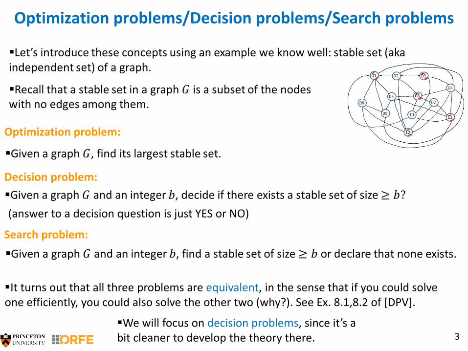
Optimization problems/Decision problems/Search problems
3
(answer to a decision question is just YES or NO)
Optimization problem:
Decision problem:
Search problem:
It turns out that all three problems are equivalent, in the sense that if you could solve one efficiently, you could also solve the other two (why?). See Ex. 8.1,8.2 of [DPV].
We will focus on decision problems, since it’s a bit cleaner to develop the theory there.
A “problem” versus a “problem instance”
4
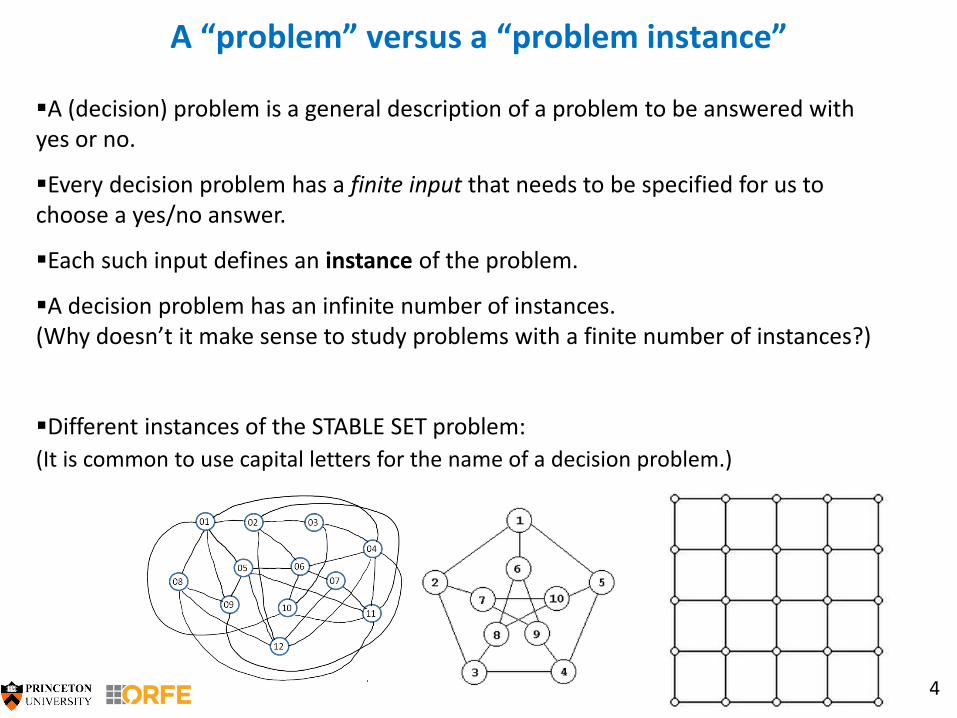
A (decision) problem is a general description of a problem to be answered with yes or no.
Every decision problem has a finite input that needs to be specified for us to choose a yes/no answer.
Each such input defines an instance of the problem.
A decision problem has an infinite number of instances. (Why doesn’t it make sense to study problems with a finite number of instances?)
Different instances of the STABLE SET problem:
(It is common to use capital letters for the name of a decision problem.)
Examples of decision problems
5
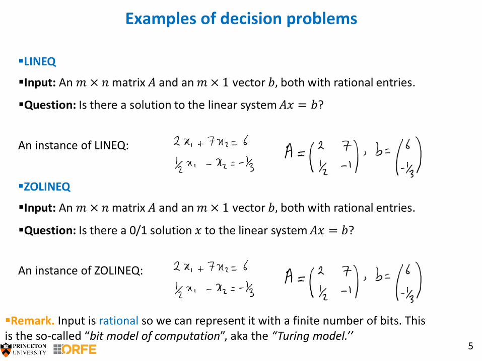
LINEQ
An instance of LINEQ:
ZOLINEQ
An instance of ZOLINEQ:
Remark. Input is rational so we can represent it with a finite number of bits. This is the so-called “bit model of computation”, aka the “Turing model.’’

Examples of decision problems
6
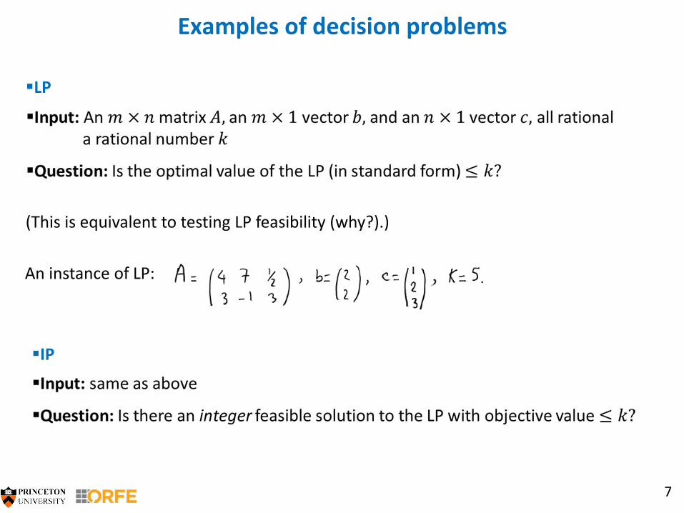
LP
An instance of LP:
(This is equivalent to testing LP feasibility (why?).)
IP
Examples of decision problems
7
LP
An instance of LP:
(This is equivalent to testing LP feasibility (why?).)
IP
Examples of decision problems
8
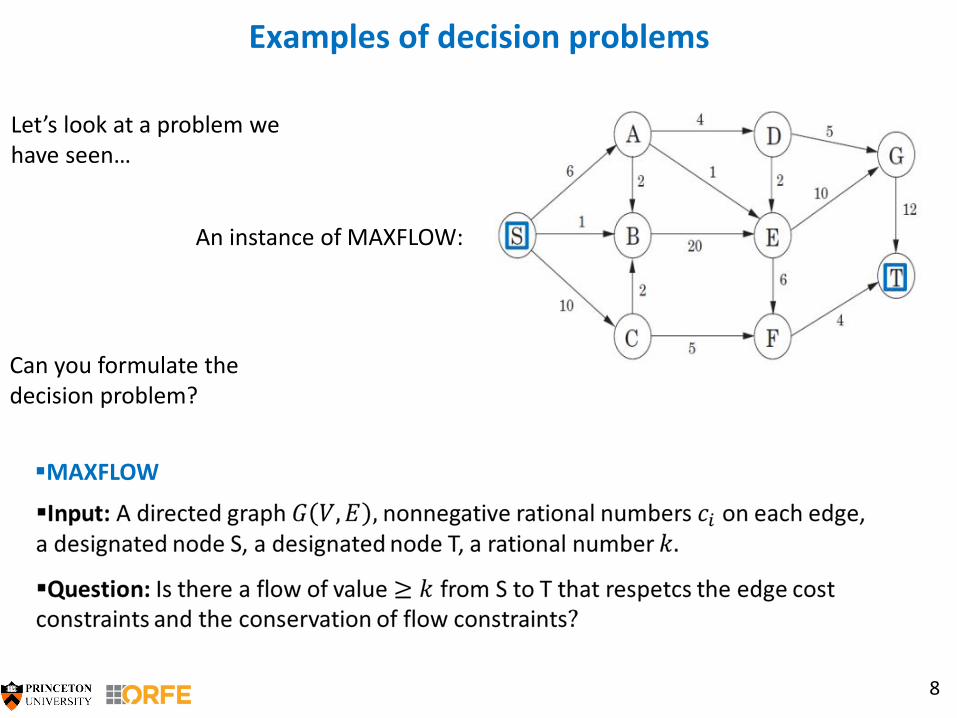
MAXFLOW
An instance of MAXFLOW:
Let’s look at a problem we have seen…
Can you formulate the decision problem?
Examples of decision problems
9
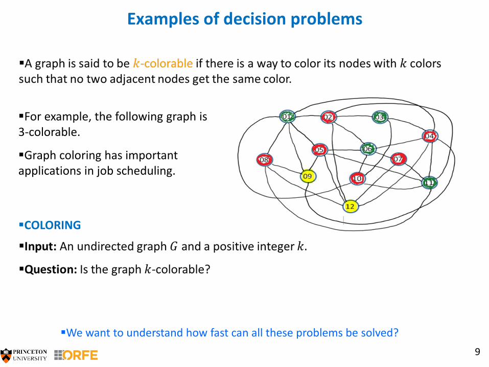
COLORING
For example, the following graph is 3-colorable.
Graph coloring has important applications in job scheduling.
We want to understand how fast can all these problems be solved?
Size of an instance
10
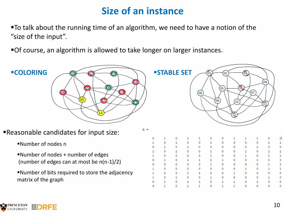
To talk about the running time of an algorithm, we need to have a notion of the “size of the input”.
Of course, an algorithm is allowed to take longer on larger instances.
COLORING STABLE SET
Reasonable candidates for input size:
Number of nodes n
Number of nodes + number of edges (number of edges can at most be n(n-1)/2)
Number of bits required to store the adjacency matrix of the graph
Size of an instance
11
In general, can think of input size as the total number of bits required to represent the input.
For example, consider our LP problem:
LP
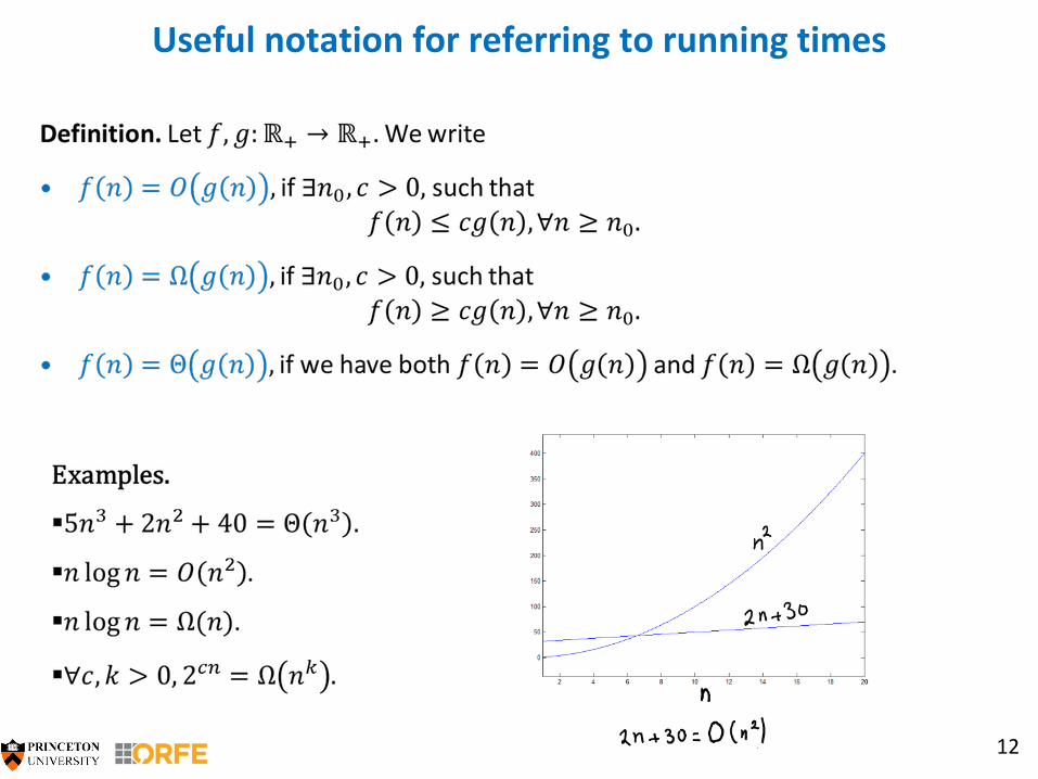
Useful notation for referring to running times
12
Polynomial-time and exponential-time algorithms
13
Something you all know: Poly-time: Exp-time:
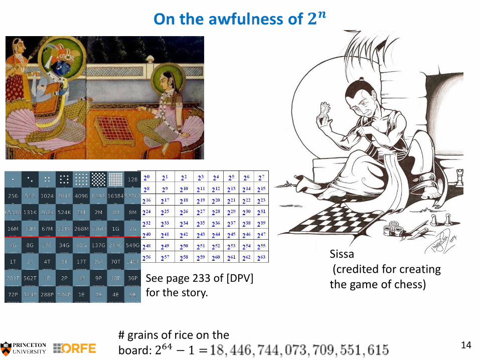
14
Sissa(credited for creating the game of chess)
See page 233 of [DPV] for the story.
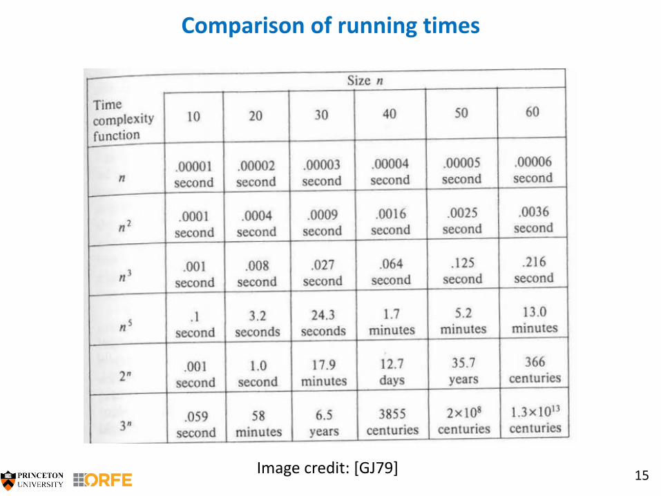
Comparison of running times
15Image credit: [GJ79]
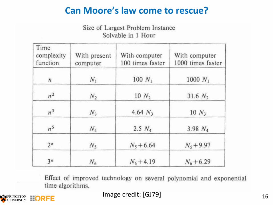
Can Moore’s law come to rescue?
16Image credit: [GJ79]
The complexity class P
17
The class of all decision problems that admit a polynomial-time algorithm.
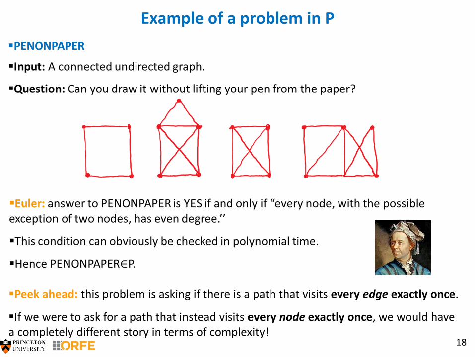
Example of a problem in P
18
PENONPAPER
Peek ahead: this problem is asking if there is a path that visits every edge exactly once.
If we were to ask for a path that instead visits every node exactly once, we would have a completely different story in terms of complexity!
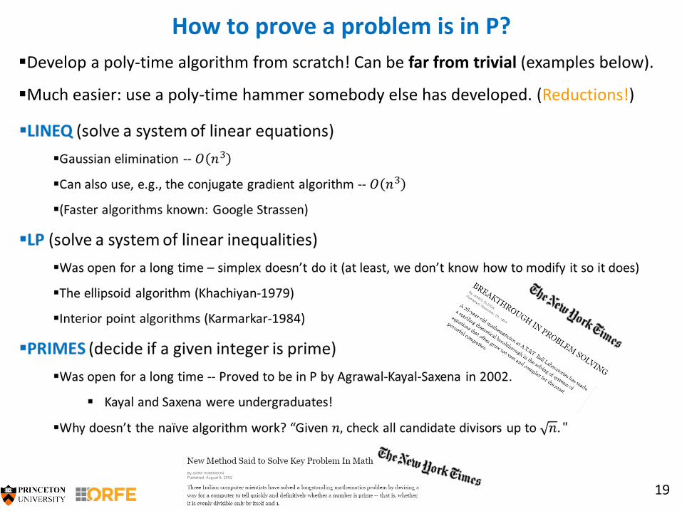
How to prove a problem is in P?
19
Develop a poly-time algorithm from scratch! Can be far from trivial (examples below).
Much easier: use a poly-time hammer somebody else has developed. (Reductions!)
An aside: Factoring
20
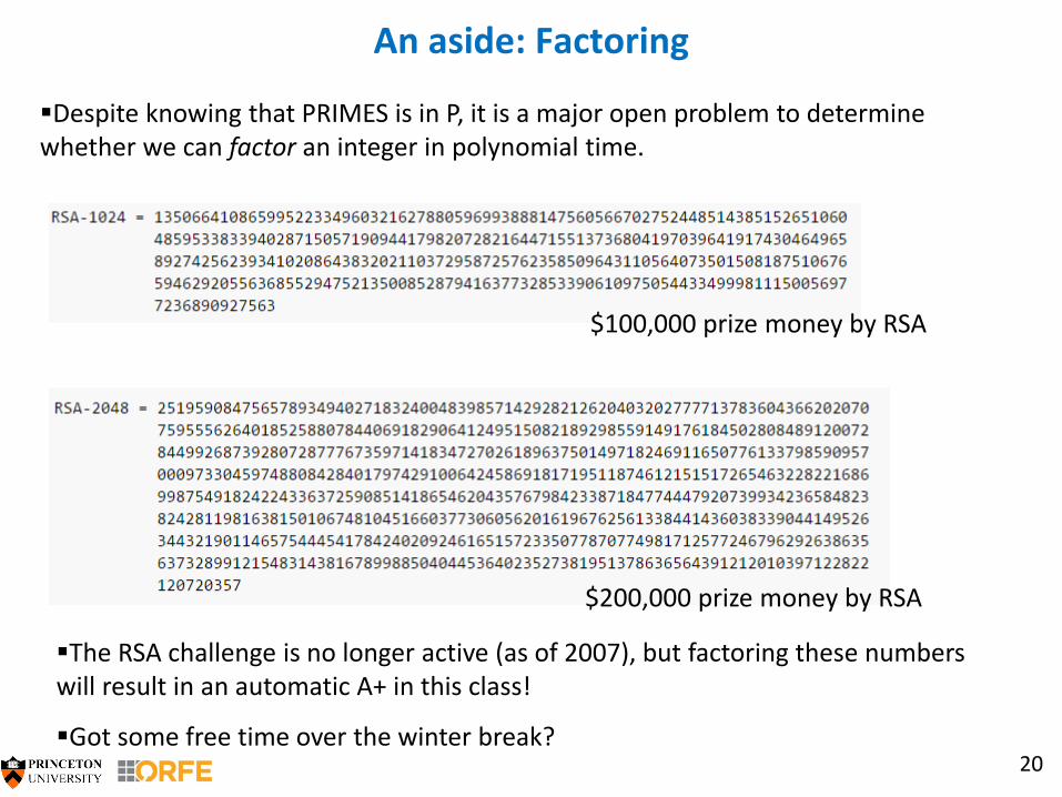
Despite knowing that PRIMES is in P, it is a major open problem to determine whether we can factor an integer in polynomial time.
$200,000 prize money by RSA
$100,000 prize money by RSA
The RSA challenge is no longer active (as of 2007), but factoring these numbers will result in an automatic A+ in this class!
Got some free time over the winter break?
Reductions
21
Many new problems are shown to be in P via a reduction to a problem that is already known to be in P.
What is a reduction?
Very intuitive idea -- A reduces to B means: “If we could do B, then we could do A.”
Being happy in life reduces to finding a good partner.
Landing a good job reduces to graduating from Princeton.
Getting an A+ in ORF 363 reduces to factoring RSA-2048.
…
Well-known joke - mathematician versus engineer boiling water:
Day 1:
Day 2:
Reductions
22
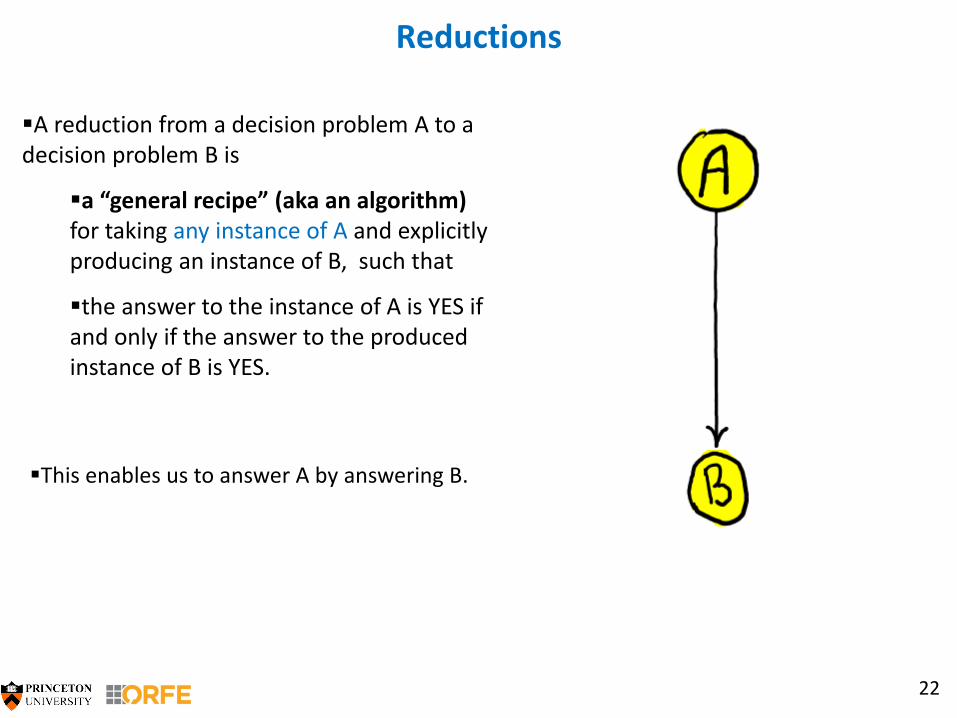
A reduction from a decision problem A to a decision problem B is
a “general recipe” (aka an algorithm)for taking any instance of A and explicitly producing an instance of B, such that
the answer to the instance of A is YES if and only if the answer to the produced instance of B is YES.
This enables us to answer A by answering B.
MAXFLOW→LP
23
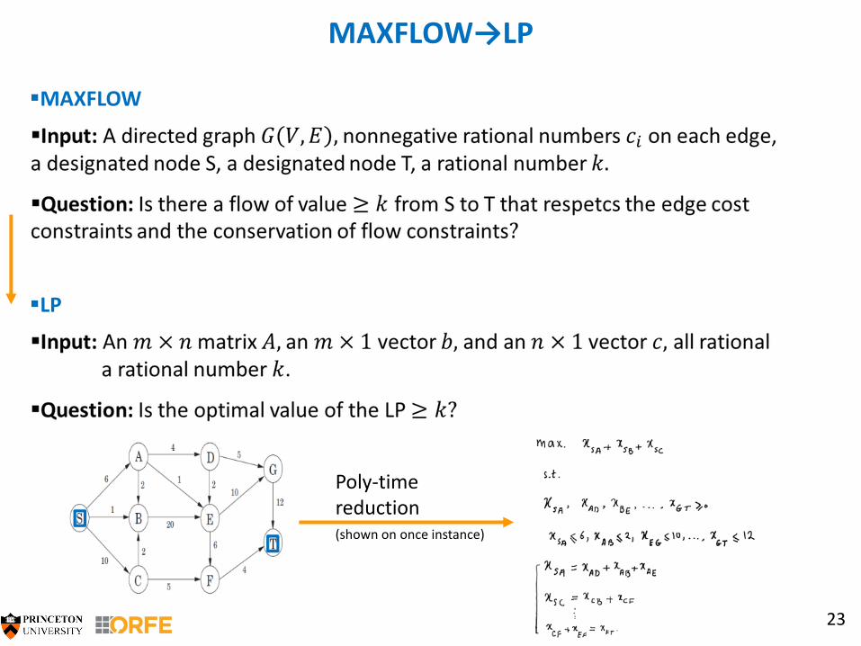
MAXFLOW
LP
Poly-timereduction(shown on once instance)
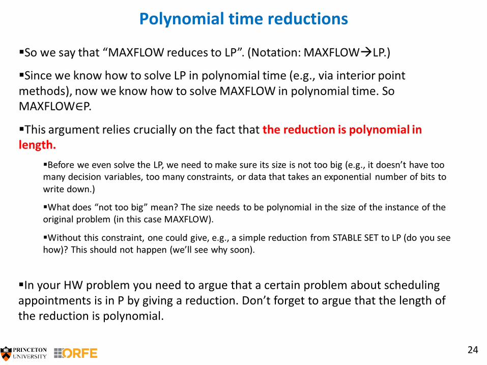
Polynomial time reductions
24
In your HW problem you need to argue that a certain problem about scheduling appointments is in P by giving a reduction. Don’t forget to argue that the length of the reduction is polynomial.
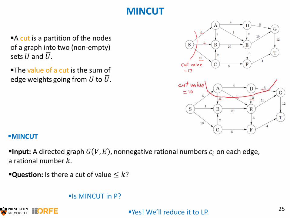
MINCUT
25
MINCUT
Is MINCUT in P?
Yes! We’ll reduce it to LP.
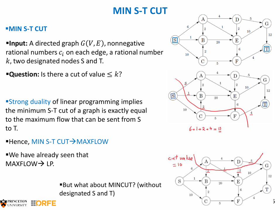
MIN S-T CUT
26
MIN S-T CUT
Strong duality of linear programming implies the minimum S-T cut of a graph is exactly equal to the maximum flow that can be sent from S to T.
Hence, MIN S-T CUTMAXFLOW
We have already seen thatMAXFLOW LP.
But what about MINCUT? (without designated S and T)
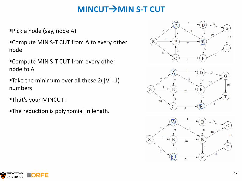
MINCUTMIN S-T CUT
27
Pick a node (say, node A)
Compute MIN S-T CUT from A to every other node
Compute MIN S-T CUT from every other node to A
Take the minimum over all these 2(|V|-1) numbers
That’s your MINCUT!
The reduction is polynomial in length.
Overall reduction
28
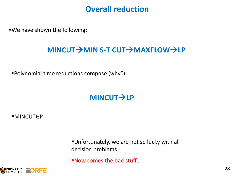
We have shown the following:
MINCUTMIN S-T CUTMAXFLOWLP
Polynomial time reductions compose (why?):
MINCUTLP
Unfortunately, we are not so lucky with all decision problems…
Now comes the bad stuff…
MAXCUT
29
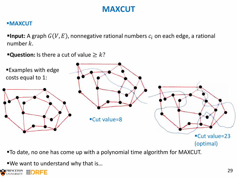
MAXCUT
Examples with edge costs equal to 1:
To date, no one has come up with a polynomial time algorithm for MAXCUT.
We want to understand why that is…
Cut value=8
Cut value=23(optimal)
The traveling salesman problem (TSP)
30
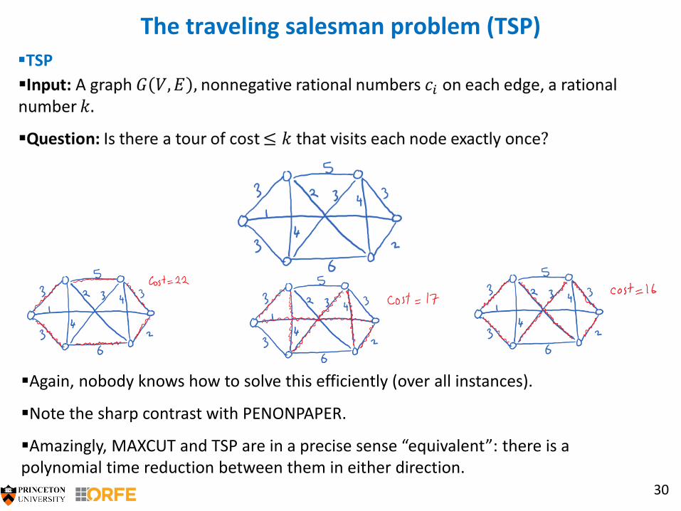
Again, nobody knows how to solve this efficiently (over all instances).
Note the sharp contrast with PENONPAPER.
Amazingly, MAXCUT and TSP are in a precise sense “equivalent”: there is a polynomial time reduction between them in either direction.
TSP
TSP
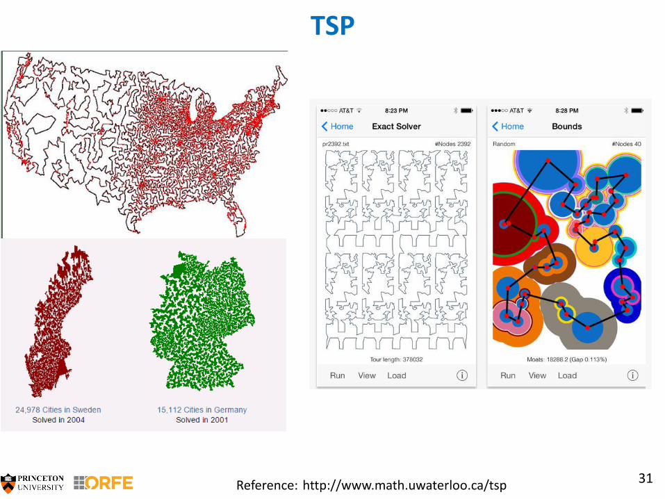
31Reference: http://www.math.uwaterloo.ca/tsp
The complexity class NP
32
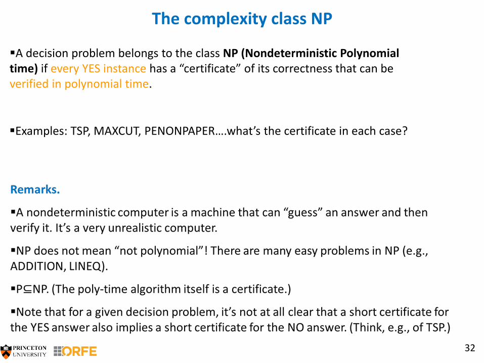
A decision problem belongs to the class NP (Nondeterministic Polynomial time) if every YES instance has a “certificate” of its correctness that can be verified in polynomial time.
Examples: TSP, MAXCUT, PENONPAPER….what’s the certificate in each case?
The complexity class NP
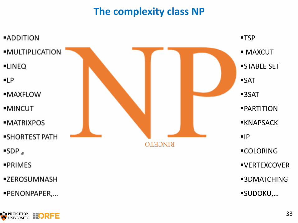
33
RINCETO
TSP
MAXCUT
STABLE SET
SAT
3SAT
PARTITION
KNAPSACK
IP
COLORING
VERTEXCOVER
3DMATCHING
SUDOKU,…
NP-hard and NP-complete problems
34
A decision problem is said to be NP-hard if every problem in NP reduces to it via a polynomial-time reduction.(roughly means “harder than all problems in NP.”)
Definition.
A decision problem is said to be NP-complete if
(i) It is NP-hard
(ii) It is in NP.
(roughly means “the hardest problems in NP.”)
Definition.
NP-hardness is shown by a reduction from a problem that’s already known to be NP-hard.
Membership in NP is shown by presenting an easily checkable certificate of the YES answer.
NP-hard problems may not be in NP (or may not be known to be in NP as is often the case.)
Remarks.
The complexity class NP
35
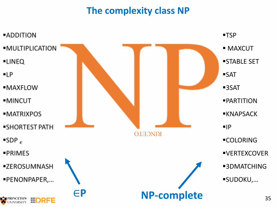
RINCETO
TSP
MAXCUT
STABLE SET
SAT
3SAT
PARTITION
KNAPSACK
IP
COLORING
VERTEXCOVER
3DMATCHING
SUDOKU,…
NP-complete
The satisfiability problem (SAT)
36
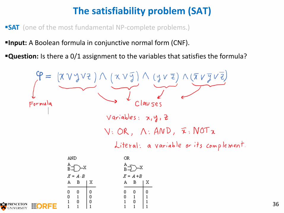
Input: A Boolean formula in conjunctive normal form (CNF).
Question: Is there a 0/1 assignment to the variables that satisfies the formula?
SAT (one of the most fundamental NP-complete problems.)
The satisfiability problem (SAT)
37
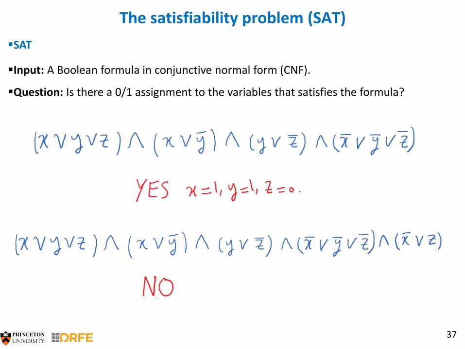
Input: A Boolean formula in conjunctive normal form (CNF).
Question: Is there a 0/1 assignment to the variables that satisfies the formula?
SAT
3SAT
38
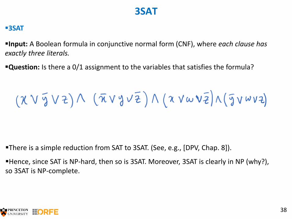
Input: A Boolean formula in conjunctive normal form (CNF), where each clause has exactly three literals.
Question: Is there a 0/1 assignment to the variables that satisfies the formula?
3SAT
There is a simple reduction from SAT to 3SAT. (See, e.g., [DPV, Chap. 8]).
Hence, since SAT is NP-hard, then so is 3SAT. Moreover, 3SAT is clearly in NP (why?), so 3SAT is NP-complete.
Reductions (again)
39
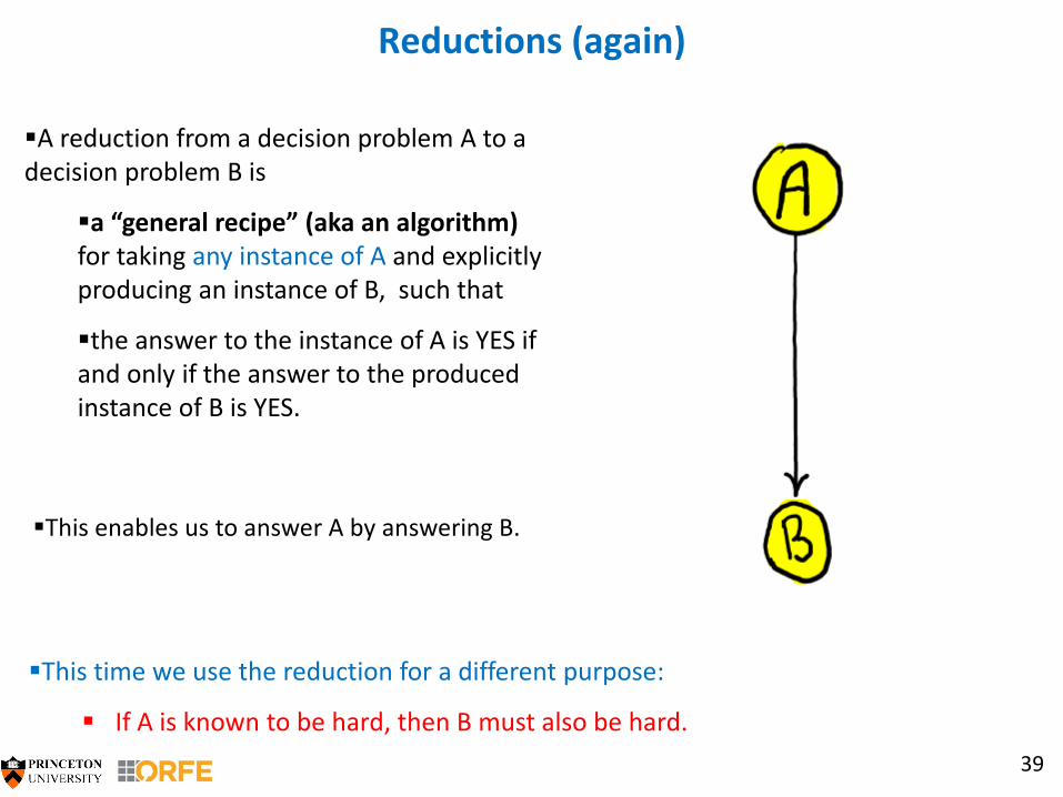
A reduction from a decision problem A to a decision problem B is
a “general recipe” (aka an algorithm)for taking any instance of A and explicitly producing an instance of B, such that
the answer to the instance of A is YES if and only if the answer to the produced instance of B is YES.
This enables us to answer A by answering B.
This time we use the reduction for a different purpose:
If A is known to be hard, then B must also be hard.
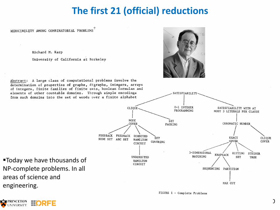
The first 21 (official) reductions
40
Today we have thousands of NP-complete problems. In all areas of science and engineering.
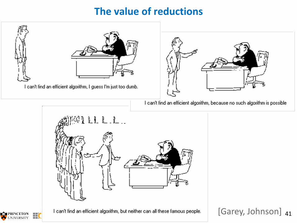
The value of reductions
41[Garey, Johnson]
Practice with reductions
42
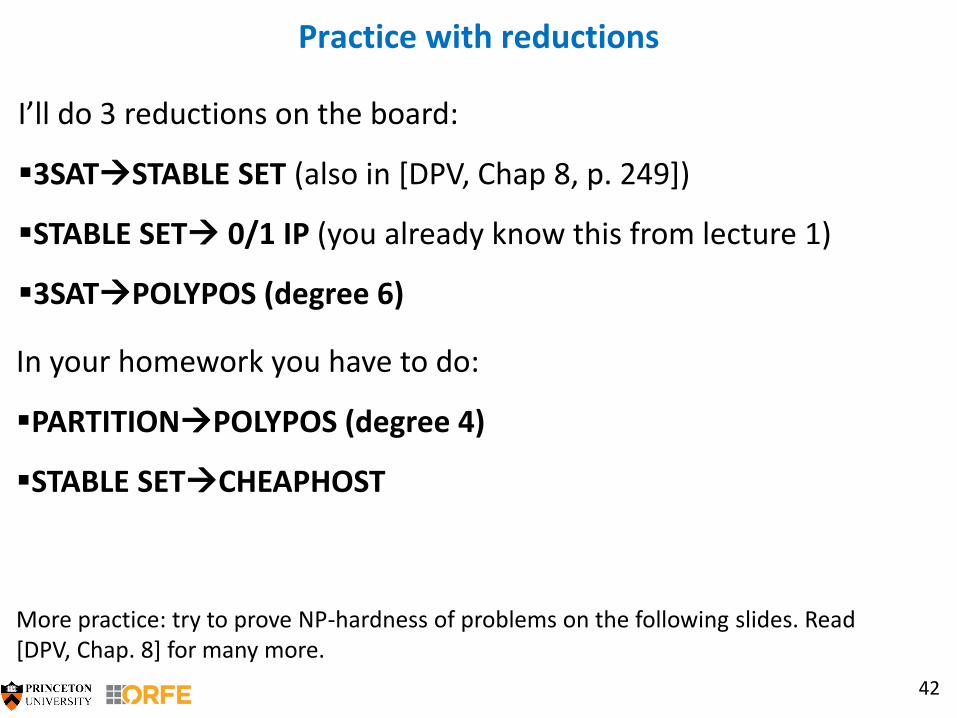
I’ll do 3 reductions on the board:
3SATSTABLE SET (also in [DPV, Chap 8, p. 249])
STABLE SET 0/1 IP (you already know this from lecture 1)
3SATPOLYPOS (degree 6)
In your homework you have to do:
PARTITIONPOLYPOS (degree 4)
STABLE SETCHEAPHOST
More practice: try to prove NP-hardness of problems on the following slides. Read [DPV, Chap. 8] for many more.
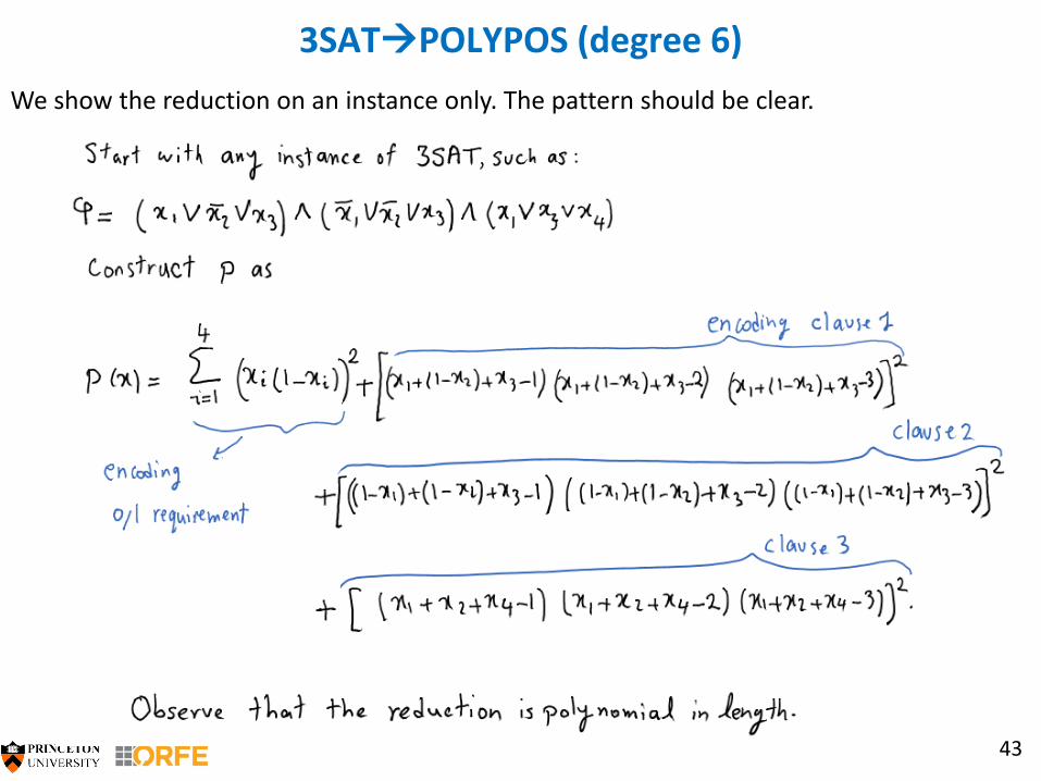
3SATPOLYPOS (degree 6)
43
We show the reduction on an instance only. The pattern should be clear.
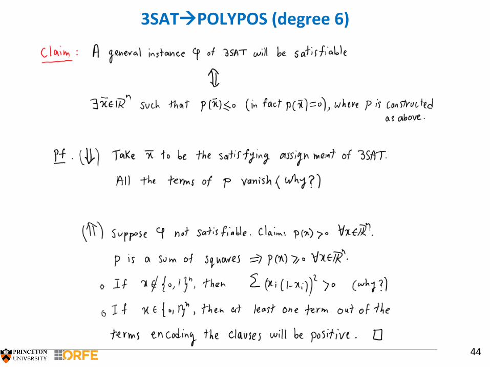
3SATPOLYPOS (degree 6)
44
The knapsack problem
45
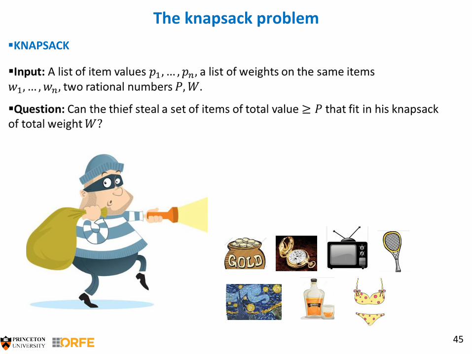
KNAPSACK
The partition problem
46
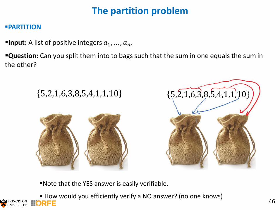
PARTITION
Note that the YES answer is easily verifiable.
How would you efficiently verify a NO answer? (no one knows)
Testing polynomial positivity
47
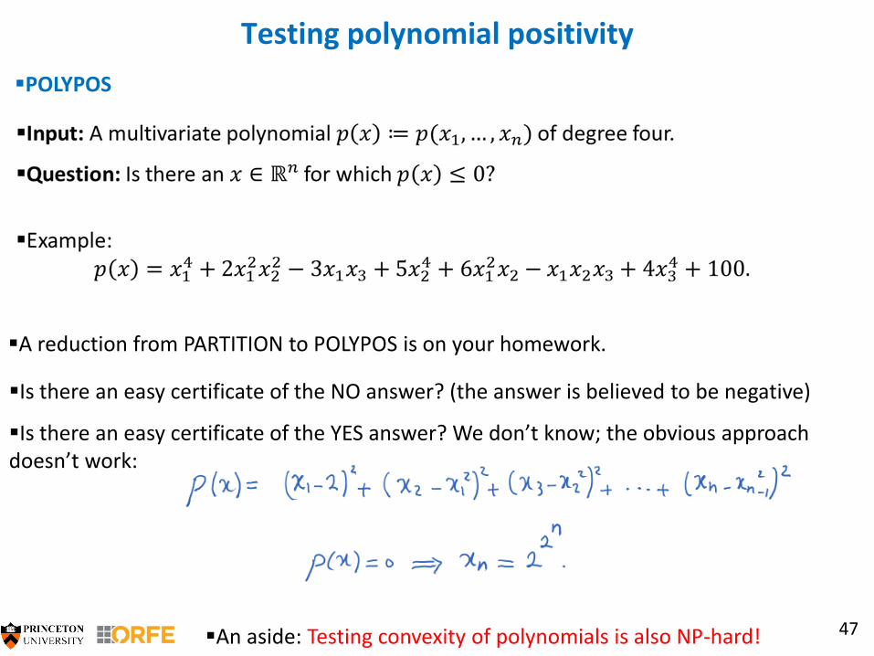
A reduction from PARTITION to POLYPOS is on your homework.
POLYPOS
Is there an easy certificate of the NO answer? (the answer is believed to be negative)
Is there an easy certificate of the YES answer? We don’t know; the obvious approach doesn’t work:
An aside: Testing convexity of polynomials is also NP-hard!
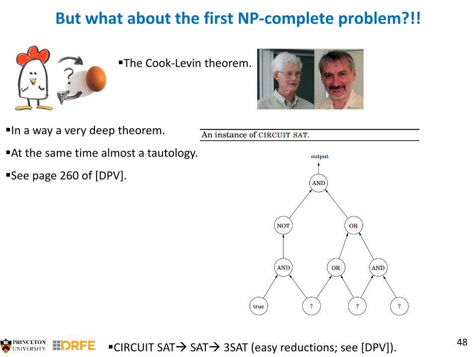
But what about the first NP-complete problem?!!
48
The Cook-Levin theorem.
In a way a very deep theorem.
At the same time almost a tautology.
See page 260 of [DPV].
CIRCUIT SAT SAT 3SAT (easy reductions; see [DPV]).
The domino effect
49
All NP-complete problems reduce to each other!
If you solve one in polynomial time, you solve ALL in polynomial time!
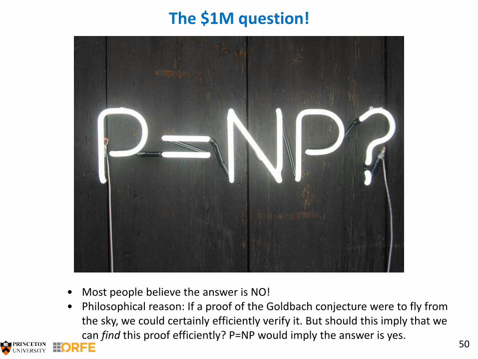
The $1M question!
50
• Most people believe the answer is NO!• Philosophical reason: If a proof of the Goldbach conjecture were to fly from
the sky, we could certainly efficiently verify it. But should this imply that we can find this proof efficiently? P=NP would imply the answer is yes.
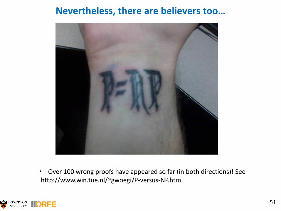
Nevertheless, there are believers too…
51
• Over 100 wrong proofs have appeared so far (in both directions)! Seehttp://www.win.tue.nl/~gwoegi/P-versus-NP.htm
Main messages…
52
Computational complexity theory beautifully classifies many problems of optimization theory as easy or hard
At the most basic level, easy means “in P”, hard means “NP-hard.”
The boundary between the two is very delicate:
MINCUT vs. MAXCUT, PENONPAPER vs. TSP, LP vs. IP, ...
Important: When a problem is shown to be NP-hard, it doesn’t mean that we should give up all hope. NP-hard problems arise in applications all the time. There are good strategies for dealing with them.
Solving special cases exactly
Heuristics that work well in practice
Using convex optimization to find bounds and near optimal solutions
Approximation algorithms – suboptimal solutions with worst-case guarantees
P=NP?
Maybe one of you guys will tell us one day.
Notes & References
53
References:
- [DPV08] S. Dasgupta, C. Papadimitriou, and U. Vazirani. Algorithms. McGraw Hill, 2008.
- [GJ79] D.S. Johnson and M. Garey. Computers and Intractability: a guide to the theory of NP-completeness, 1979.
- [BT00] V.D. Blondel and J.N. Tsitsiklis. A survey of computational complexity results in systems and control. Automatica, 2000.
Notes:
- Relevant reading for this lecture is Chapter 8 of [DPV08].